commonly used frequency measures in health care used frequency measures in health care 1 ......

CHAPTER 1

Commonly Used FrequencyMeasures in Health Care

1

KEY TERMS Variable Postneonatal mortality rateFrequency distribution Infant mortality rateRate Morbidity ratesRatio Incidence rateProportion Prevalence rateDichotomous variables Point prevalence rateConfounding factor Risk ratiosConfounding variable Relative riskMortality rates Odds ratio

Crude death rate Attributable riskAge-specific death rate Kaplan Meier method

(ASDR) Kaplan-Meier survival Age-adjusted death rate analysisStandard mortality ratio (SMR)Race-specific death rateSex-specific death rateCause-specific death rateCase fatality rateProportionate mortality ratio (PMR)Maternal mortality rateNeonatal mortality rate

LEARNING At the conclusion of this chapter, you should be able to:OBJECTIVES 1. Define key terms.

2. Calculate measures of morbidity, mortality, and risk of disease forhealth care facilities and communities.

3. Identify variables that affect morbidity and mortality rates over time.

1290.ch01 4/21/05 11:24 AM

4. Adjust measures of morbidity and mortality by both the direct and in-direct methods of standardization.

5. After adjustment, compare health care facility mortality/morbidityrates with community, state, and/or national rates.

6. Calculate risk of disease between groups.7. Conduct survival analysis for tumor registries and clinical trials.

It is often said that hospitals and other types of health care facilities are data rich but infor-mation poor. There are many types of databases within the facility, many contained withinthe organization’s information warehouse. Information warehouses contain both clinical andfinancial information. It is the job of the health information management professional toturn the data contained in these databases into information that can be used by physicians,administrators, and other interested parties. The health information management profes-sional can become an invaluable member of the health care team by providing data that arepresented in a meaningful way and by presenting data that have been analyzed to serve aspecific medical or clinical need. Some typical questions might be:

• What are the top 25 medical and top 10 surgical diagnosis-related groups (DRGs) forinpatient discharges from our facility?

• Which medical/surgical services admit the most patients?• Is the average length of stay (ALOS) for these DRGs significantly different from the

national ALOS for these DRGs?• How do our charges compare with national charges? How does our reimbursement

compare with our costs?• What geographical area does the health care facility serve?• How many patients were admitted to the facility by payer? What is the number of in-

patient service days by payer? What are the average charges by payer?• How do lengths of stay (LOSs) compare by physician?• How many patients acquired nosocomial infections?

In the course of this text we will answer these questions. We will learn how to use de-scriptive statistics to describe patient populations, how to analyze clinical data for signifi-cant differences and relationships, and how to present data in graphic form. Our goal is tocollect, analyze, and interpret clinical information for both clinical and administrative healthcare decision makers. We will begin our discussion of clinical data analysis by reviewingmorbidity and mortality measures that are often used to describe patient and communitypopulations.

INTRODUCTION TO FREQUENCY DISTRIBUTIONS

In health care, we deal with vast quantities of clinical data. Since it is very difficult to lookat data in raw form, data are summarized into frequency distributions. A frequency distri-

2 CHAPTER 1 COMMONLY USED FREQUENCY MEASURES IN HEALTH CARE

1290.ch01 4/21/05 11:24 AM

bution shows the values that a variable can take and the number of observations associatedwith each value. A variable is a characteristic or property that may take on different values.Height, weight, sex, and third-party payer are examples of variables.

For example, suppose we are studying the variable patient LOS in the pediatric unit. Toconstruct a frequency distribution, we first list all the values that LOS can take, from thelowest observed value to the highest. We then enter the number of observations (frequen-cies) corresponding to a given LOS. Table 1–1 illustrates what the resulting frequency dis-tribution looks like. Note that all values for LOS between the lowest and highest are listed,even though there may not be any observations for some of the values. Each column of thedistribution is properly labeled; the total is given in the bottom row. We can also display afrequency distribution by categories into which a variable may fall. Table 1–2 shows a fre-quency distribution for the number of patients discharged from Critical Care Hospital by re-ligion, a variable composed of categories. The proportion for each category is also displayedin the table. The sum of the proportions for each category is equal to 1.0. We will examinefrequency distributions in greater detail in Chapter 4.

Introduction to Frequency Distributions 3

Table 1–1 Frequency Distribution for Patient Lengthof Stay (LOS), Pediatric Unit

LOS in Days No. of Patients

1 22 23 04 65 66 117 68 59 3

10 1Total 42

Table 1–2 Frequency Distribution of Number of PatientsDischarged from Critical Care Hospital by Religion, July20xx

Religion Number of Discharges Proportion

Protestant 422 0.48Catholic 315 0.36Jewish 20 0.02Other 127 0.14Total 884 1.00

1290.ch01 4/21/05 11:24 AM

RATIOS, PROPORTIONS, AND RATES

Variables often have only two possible categories, such as alive or dead, or male or female.Variables having only two possible categories are called dichotomous. The frequency mea-sures used with dichotomous variables are ratios, proportions, and rates. All three mea-sures are based on the same formula:

ratio, proportion, rate � x/y � 10n

In this formula, x and y are the two quantities being compared, and x is divided by y. 10n

is read as “10 to the nth power.” The size of 10n may equal, for example, 1, 10, 100, or 1,000,depending on the value of n:

100 � 1

101 � 10

102 � 10 � 10 � 100

103 � 10 � 10 � 10 � 1,000

Ratios

In a ratio, the values of a variable, such as sex (x � female, y � male), may be expressed sothat x and y are completely independent of each other, or x may be included in y. For exam-ple, the sex of patients discharged from a hospital could be compared in either of two ways:

Female/male or x/y

Female/(male � female) or x/(x � y)

In the first option, x is completely independent of y, and the ratio represents the numberof female discharges compared to the number of male discharges. In the second option, x isa proportion of the whole, x � y. The ratio represents the number of female discharges com-pared to the total number of discharges. Both expressions are considered ratios.

How, then, would you calculate the female-to-male ratio for a hospital that discharged 457women and 395 men during the month of July? The procedure for calculating a ratio is out-lined in Exhibit 1–1.

Proportions

A proportion is a particular type of ratio. A proportion is a ratio in which x is a portion ofthe whole, x � y. In a proportion, the numerator is always included in the denominator. Ex-hibit 1–2 outlines the procedure for determining the proportion of hospital discharges forthe month of July that were female.


1290.ch01 4/21/05 11:24 AM

Rates

Rates are a third type of frequency measure. In health care, rates are often used to measurean event over time and are sometimes used as performance improvement measures. The ba-sic formula for a rate is:

No. of cases or events occurring during a given time period � 10n

No. of cases or population at risk during same time period

or

Total number of times something did happen � 10n

Total number of times something could happen

Ratios, Proportions, and Rates 5

Exhibit 1–1 Calculation of a Ratio: Discharges for July 20xx

1. Define x and y.x � number of female discharges y � number of male discharges

2. Identify x and y.x � 457 y � 395

3. Set up the ratio x/y.457/395

4. Reduce the fraction so that either x or y equals 1.1.16/1

There were 1.16 female discharges for every male discharge.

Exhibit 1–2 Calculation of a Proportion: Discharges for July 20xx

1. Define x and y.x � number of female discharges y � number of male discharges

2. Identify x and y.x � 457y � 395

3. Set up the proportionx/(x � y) 457/(457 � 395) � 457/852

4. Reduce the fraction so that either x or x � y equals 1.0.54/1.00

The proportion of discharges that were female is 0.54.

1290.ch01 4/21/05 11:24 AM

In inpatient facilities, there are many commonly computed rates. In computing the Cae-sarean section rate, we count the number of Caesarean sections (C-sections) performed dur-ing a given period of time; this value is placed in the numerator. The number of cases orpopulation at risk is the number of women who delivered during the same time period; thisnumber is placed in the denominator. By convention, inpatient hospital rates are calculatedas the rate per 100 cases (10n � 102 � 10 � 10 � 100) and are expressed as a percentage.The method for calculating the hospital C-section rate is presented in Exhibit 1–3.


Exhibit 1–3 Calculation of C-Section Rate for July 20xx

For the month of July, 23 C-sections were performed; during the same time period, 149 women delivered.What is the C-section rate for the month of July?

1. Define the variable of interest (numerator) and population or number of cases at risk (denominator).Numerator: total number of C-sections performed in JulyDenominator: total number of women who delivered in July, including C-sections

2. Identify the numerator and denominator.Numerator: 23 Denominator: 149

3. Set up the rate.23/149

4. Divide the numerator by the denominator, and multiply by 100 (10n � 102).(23/149) � 100 � 15.4%.

The C-section rate for the month of July is 15.4%.

POPULATION-BASED MORTALITY MEASURES

As the profession of health information management moves into integrated health care de-livery systems and assumes more prominence in managed care organizations, it becomesmore important to be familiar with community-based mortality and morbidity data. Thistype of information is often used in planning health services, such as number of inpatientfacilities, type of outpatient facilities, and number or size of managed care plans for a givencommunity, as well as for developing managed care contracts with hospitals and physicians.

Crude Death Rate

The crude death rate is a measure of the actual or observed mortality in a given population.Crude rates apply to a population without regard to characteristics of the population, suchas the distribution of age or sex. The crude death rate is the starting point for further devel-opment of adjusted rates. It measures the proportion of a population that has died during aspecific period of time, usually one year, or the number of deaths per 1,000 in a communityfor a given period of time. The crude death rate is calculated as follows (the midinterval pop-

1290.ch01 4/21/05 11:24 AM

ulation is the estimated population of a given community at the midpoint of the time frameunder study):

Total deaths during a given time interval � 10n � deaths per 10n

Estimated midinterval population

In calculating the crude death rate, the power of n is usually equal to the value that willresult in a value greater than 1. This allows for easier interpretation of the rate—a death rateof less than 1 per 100 is not very meaningful. For example, the 2004 midyear population ofAnytown, USA, is 1,996,355; 275 deaths occurred in 2004. The power of n that will resultin a whole number is 4; 104 � 10 � 10 � 10 � 10 � 10,000. The crude death rate is cal-culated as follows:

(275 � 10,000)/1,996,355 � 2,750,000/1,996,355 � 1.38 deaths per 10,000

When analyzing crude death rates, or any type of rate, it is important to remember thatthese events do not occur in a vacuum. When analyzing any data set, we need to rememberthat the data do not stand alone, but reflect trends in the environment. Trends in death ratescan be influenced by three variables: time, place, and person. Examples of time, place, andperson variables are outlined in Exhibit 1–4. An example of how trended data may be af-fected by time, place, and person variables is presented in Figure 1–1. The line graph showsthat the number of newly diagnosed acquired immune deficiency syndrome (AIDS) casessteadily increased from 1983 to 1992; then a rather dramatic increase occurred in 1993,

Population-Based Mortality Measures 7

Exhibit 1–4 Variables Affecting Trends in Community Morbidity and Mortality

• TimeTransition from International Classification of Diseases, 9th Revision (ICD-9) to ICD-10 in coding

of death certificates Improvements in medical technology Earlier detection and diagnosis of disease

• PlaceChanges in environments International and intranational differences in medical technology and the use of medical technology Diagnostic practices of physicians Variation in physician practice patterns by region

• PersonAge Sex Ethnicity Social habits (smoking, diet, alcohol) Genetic background Emotional and mental characteristics

1290.ch01 4/21/05 11:24 AM

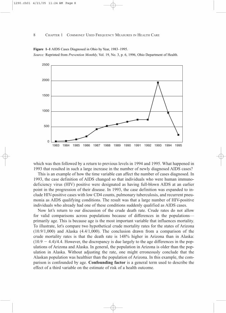
which was then followed by a return to previous levels in 1994 and 1995. What happened in1993 that resulted in such a large increase in the number of newly diagnosed AIDS cases?

This is an example of how the time variable can affect the number of cases diagnosed. In1993, the case definition of AIDS changed so that individuals who were human immuno-deficiency virus (HIV) positive were designated as having full-blown AIDS at an earlierpoint in the progression of their disease. In 1993, the case definition was expanded to in-clude HIV-positive cases with low CD4 counts, pulmonary tuberculosis, and recurrent pneu-monia as AIDS qualifying conditions. The result was that a large number of HIV-positiveindividuals who already had one of these conditions suddenly qualified as AIDS cases.

Now let’s return to our discussion of the crude death rate. Crude rates do not allow for valid comparisons across populations because of differences in the populations—primarily age. This is because age is the most important variable that influences mortality.To illustrate, let's compare two hypothetical crude mortality rates for the states of Arizona(10.9/1,000) and Alaska (4.4/1,000). The conclusion drawn from a comparison of the crude mortality rates is that the death rate is 148% higher in Arizona than in Alaska: (10.9 � 4.4)/4.4. However, the discrepancy is due largely to the age differences in the pop-ulations of Arizona and Alaska. In general, the population in Arizona is older than the pop-ulation in Alaska. Without adjusting the rate, one might erroneously conclude that theAlaskan population was healthier than the population of Arizona. In this example, the com-parison is confounded by age. Confounding factor is a general term used to describe theeffect of a third variable on the estimate of risk of a health outcome.


2500

2000

1500

1000

500

01983 1984 1985 1986 1987 1988 1989 1990 1991 1992 1993 19951994

Figure 1–1 AIDS Cases Diagnosed in Ohio by Year, 1983–1995.

Source: Reprinted from Prevention Monthly, Vol. 19, No. 3, p. 6, 1996, Ohio Department of Health.

1290.ch01 4/21/05 11:24 AM

Confounding occurs when a third factor related to outcome is differentially distributedacross the levels (or categories) of a variable of interest. When this happens, we must takemeasures to separate the effect of the confounding variable—in this case, age—from theeffect of the variable of interest. We can accomplish this by selecting subjects to be com-pared so that they are matched with respect to the confounding variables, or by using sta-tistical adjustments during analysis to remove the effect of the confounding variable. Forexample, review the data in Table 1–3. Analysis of the data reveals that the overall crude rateis less for blacks than for whites but that the age-specific death rate for blacks is higher thanthe rates for whites in every age group. Why is there such a contradiction? It is because the2001 population of the state of Georgia consisted of old whites and young blacks—33.7%of the white population was 24 years old or younger, and 43.1% of the black population was24 years old or younger.


Table 1–3 Age-Specific Death Rates per 1,000 Population, State of Georgia, 2001

Race Crude Rate � 1 Yr. 1–4 Yrs. 5–14 Yrs. 15–24 Yrs. 25–44 Yrs. 45–64 Yrs. � 65 Yrs.

White 8.15 6.25 0.42 0.18 0.92 1.49 6.53 51.25Black 7.04 13.33 0.51 0.24 1.04 2.54 10.68 59.02

Source: United States Department of Health and Human Services, Centers for Disease Control and Prevention (CDC), CDCOn-line Database, wonder.cdc.gov.

Age-Specific Death Rates

In Table 1–3, we see the age-specific death rates (ASDR) for both whites and blacks. TheASDR is calculated as follows:

No. of deaths in the age group of interest � 10n

Estimated mid-period population in the age group of interest

Age-Adjusted Death Rates

Age-adjusted death rates are used when there are differences in the age distribution for thepopulations that are being compared. In Table 1–4, you can see that the population propor-tions for each age group vary slightly by race. For example, the proportion of whites that areolder than age 65 is 0.115 (11.5%) and the proportion of blacks that are older than 65 is0.064 (6.4%). When we adjust the crude rate for age, we are constructing a summary ratethat is free of age bias. In Table 1–4, the ASDR for each age group is expressed as a per-centage. There are two methods for adjusting the crude death rate—direct and indirect. Wewill first discuss the direct method of standardization.

1290.ch01 4/21/05 11:24 AM

Direct Standardization

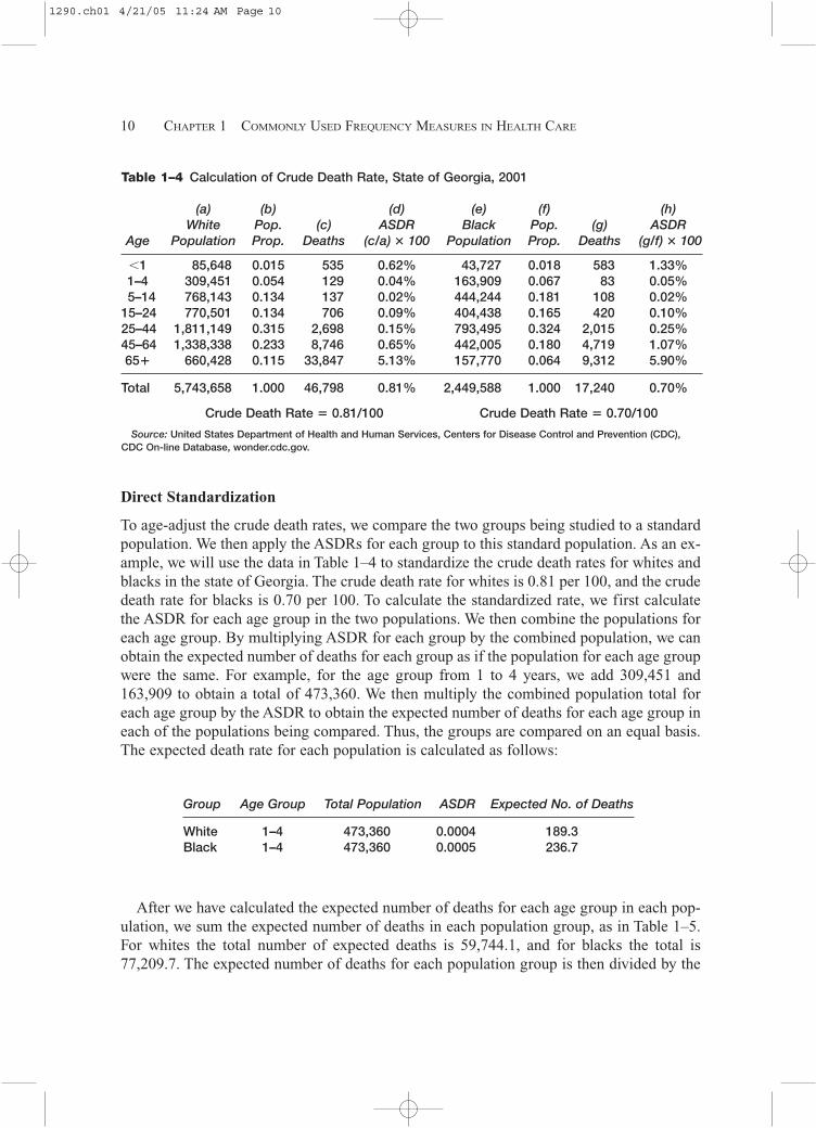
To age-adjust the crude death rates, we compare the two groups being studied to a standardpopulation. We then apply the ASDRs for each group to this standard population. As an ex-ample, we will use the data in Table 1–4 to standardize the crude death rates for whites andblacks in the state of Georgia. The crude death rate for whites is 0.81 per 100, and the crudedeath rate for blacks is 0.70 per 100. To calculate the standardized rate, we first calculatethe ASDR for each age group in the two populations. We then combine the populations foreach age group. By multiplying ASDR for each group by the combined population, we canobtain the expected number of deaths for each group as if the population for each age groupwere the same. For example, for the age group from 1 to 4 years, we add 309,451 and163,909 to obtain a total of 473,360. We then multiply the combined population total foreach age group by the ASDR to obtain the expected number of deaths for each age group ineach of the populations being compared. Thus, the groups are compared on an equal basis.The expected death rate for each population is calculated as follows:


Table 1–4 Calculation of Crude Death Rate, State of Georgia, 2001

(a) (b) (d) (e) (f) (h)White Pop. (c) ASDR Black Pop. (g) ASDR

Age Population Prop. Deaths (c/a) � 100 Population Prop. Deaths (g/f) � 100

�1 85,648 0.015 535 0.62% 43,727 0.018 583 1.33%1–4 309,451 0.054 129 0.04% 163,909 0.067 83 0.05%5–14 768,143 0.134 137 0.02% 444,244 0.181 108 0.02%

15–24 770,501 0.134 706 0.09% 404,438 0.165 420 0.10%25–44 1,811,149 0.315 2,698 0.15% 793,495 0.324 2,015 0.25%45–64 1,338,338 0.233 8,746 0.65% 442,005 0.180 4,719 1.07%65� 660,428 0.115 33,847 5.13% 157,770 0.064 9,312 5.90%

Total 5,743,658 1.000 46,798 0.81% 2,449,588 1.000 17,240 0.70%

Crude Death Rate � 0.81/100 Crude Death Rate � 0.70/100

Source: United States Department of Health and Human Services, Centers for Disease Control and Prevention (CDC), CDC On-line Database, wonder.cdc.gov.

Group Age Group Total Population ASDR Expected No. of Deaths

White 1–4 473,360 0.0004 189.3Black 1–4 473,360 0.0005 236.7

After we have calculated the expected number of deaths for each age group in each pop-ulation, we sum the expected number of deaths in each population group, as in Table 1–5.For whites the total number of expected deaths is 59,744.1, and for blacks the total is77,209.7. The expected number of deaths for each population group is then divided by the

1290.ch01 4/21/05 11:24 AM

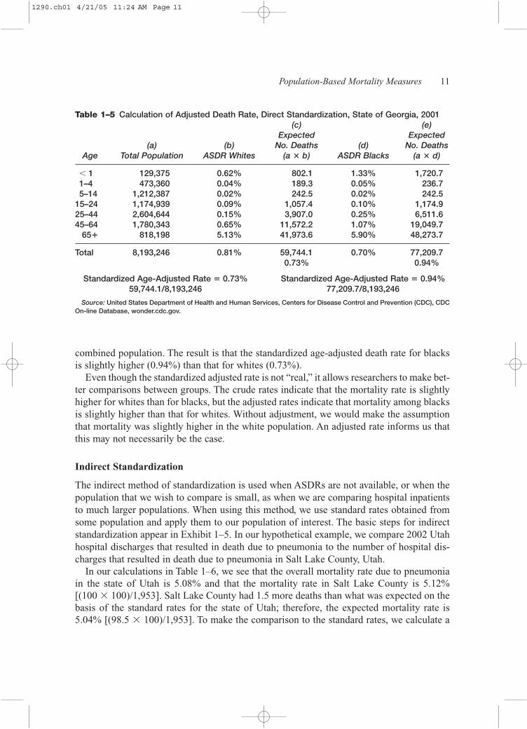
combined population. The result is that the standardized age-adjusted death rate for blacksis slightly higher (0.94%) than that for whites (0.73%).

Even though the standardized adjusted rate is not “real,” it allows researchers to make bet-ter comparisons between groups. The crude rates indicate that the mortality rate is slightlyhigher for whites than for blacks, but the adjusted rates indicate that mortality among blacksis slightly higher than that for whites. Without adjustment, we would make the assumptionthat mortality was slightly higher in the white population. An adjusted rate informs us thatthis may not necessarily be the case.

Indirect Standardization

The indirect method of standardization is used when ASDRs are not available, or when thepopulation that we wish to compare is small, as when we are comparing hospital inpatientsto much larger populations. When using this method, we use standard rates obtained fromsome population and apply them to our population of interest. The basic steps for indirectstandardization appear in Exhibit 1–5. In our hypothetical example, we compare 2002 Utahhospital discharges that resulted in death due to pneumonia to the number of hospital dis-charges that resulted in death due to pneumonia in Salt Lake County, Utah.

In our calculations in Table 1–6, we see that the overall mortality rate due to pneumoniain the state of Utah is 5.08% and that the mortality rate in Salt Lake County is 5.12% [(100 � 100)/1,953]. Salt Lake County had 1.5 more deaths than what was expected on thebasis of the standard rates for the state of Utah; therefore, the expected mortality rate is5.04% [(98.5 � 100)/1,953]. To make the comparison to the standard rates, we calculate a


Table 1–5 Calculation of Adjusted Death Rate, Direct Standardization, State of Georgia, 2001(c) (e)

Expected Expected(a) (b) No. Deaths (d) No. Deaths

Age Total Population ASDR Whites (a � b) ASDR Blacks (a � d)

� 1 129,375 0.62% 802.1 1.33% 1,720.71–4 473,360 0.04% 189.3 0.05% 236.75–14 1,212,387 0.02% 242.5 0.02% 242.5

15–24 1,174,939 0.09% 1,057.4 0.10% 1,174.925–44 2,604,644 0.15% 3,907.0 0.25% 6,511.645–64 1,780,343 0.65% 11,572.2 1.07% 19,049.7

65� 818,198 5.13% 41,973.6 5.90% 48,273.7

Total 8,193,246 0.81% 59,744.1 0.70% 77,209.70.73% 0.94%

Standardized Age-Adjusted Rate � 0.73% Standardized Age-Adjusted Rate � 0.94%59,744.1/8,193,246 77,209.7/8,193,246


1290.ch01 4/21/05 11:24 AM

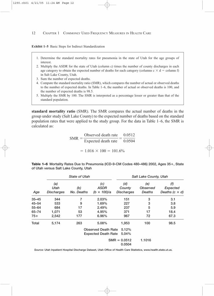
standard mortality ratio (SMR). The SMR compares the actual number of deaths in thegroup under study (Salt Lake County) to the expected number of deaths based on the standardpopulation rates that were applied to the study group. For the data in Table 1–6, the SMR iscalculated as:


Table 1–6 Mortality Rates Due to Pneumonia (ICD-9-CM Codes 480–486) 2002, Ages 35�, Stateof Utah versus Salt Lake County, Utah

State of Utah Salt Lake County, Utah

(a) (c) (d) (e) (f) Utah (b) ASDR County Observed Expected

Age Discharges No. Deaths (b � 100)/a Discharges Deaths Deaths (c � d)

35–45 344 7 2.03% 151 3 3.145–54 533 9 1.69% 227 3 3.855–64 684 17 2.49% 237 5 5.965–74 1,071 53 4.95% 371 17 18.475� 2,542 177 6.96% 967 72 67.3

Total 5,174 263 5.08% 1,953 100 98.5

Observed Death Rate 5.12%Expected Death Rate 5.04%

SMR � 0.0512 1.10160.0504

Source: Utah Inpatient Hospital Discharge Dataset, Utah Office of Health Care Statistics, www.health.state.ut.us.

SMR �Observed death rate

�0.0512

Expected death rate 0.0504

� 1.016 � 100 � 101.6%

Exhibit 1–5 Basic Steps for Indirect Standardization

1. Determine the standard mortality rates for pneumonia in the state of Utah for the age groups of interest.

2. Multiply the ASDR for the state of Utah (column c) times the number of county discharges in eachage category to obtain the expected number of deaths for each category (columns c � d � column f)in Salt Lake County, Utah.

3. Sum the number of expected deaths. 4. Compute the standard mortality ratio (SMR), which compares the number of actual or observed deaths

to the number of expected deaths. In Table 1–6, the number of actual or observed deaths is 100, andthe number of expected deaths is 98.5.

5. Multiply the SMR by 100. The SMR is interpreted as a percentage lesser or greater than that of thestandard population.

1290.ch01 4/21/05 11:24 AM

If the calculated SMR is equal to 100, the number of observed deaths is the same as thenumber of expected deaths. If the SMR is greater than 100, the number of observed deathsis greater than the number of expected deaths. The interpretation of the SMR is that SaltLake County’s pneumonia death rate is 1% greater than that for the state of Utah. Stated an-other way, the death rate is 1% greater than what would be expected on the basis of the mor-tality rates due to pneumonia for the entire state of Utah.

In summary, rates are adjusted to remove the effect of the confounding factor for whichthe adjustment has been made—in this case, age. However, it is always necessary to calcu-late the crude rate because this represents the actual event. An adjusted rate is used for com-parative purposes; adjusted rates do not reveal the underlying raw data that are shown by thecrude rates.

Race- and Sex-Specific Death Rates

Mortality rates may be calculated for any variable of interest, such as race or sex, using thesame basic formula specified for calculating the crude death rate. Historically in the UnitedStates, men have had higher mortality rates than women, but the gap may be narrowing. In1995, the U.S. sex-specific rate was 9.2 per 1,000 for men and 8.6 per 1,000 for women.However, in 2001, the sex-specific death rate for men was 8.45 per 1,000 for men and 8.49per 1,000 for women (Table 1–7).


Table 1–7 Sex-Specific Death Rates, United States, 2001

Women Men

Rate/ Rate/Age Population Deaths 1,000 Population Deaths 1,000

Under 1 Year 1,968,011 12,091 6.14 2,057,922 15,477 7.521–4 years 7,491,412 2,208 0.29 7,841,553 2,899 0.375–9 years 9,861,089 1,366 0.14 10,347,035 1,727 0.1710–14 years 10,199,195 1,561 0.15 10,711,245 2,441 0.2315–19 years 9,847,662 3,789 0.38 10,423,650 9,766 0.9420–24 years 9,630,499 4,500 0.47 10,080,924 14,197 1.4125–34 years 19,698,788 12,926 0.66 20,116,087 28,757 1.4335–44 years 22,675,474 33,510 1.48 22,464,812 58,164 2.5945–54 years 19,971,971 63,217 3.17 19,256,395 104,848 5.4455–64 years 13,160,005 99,181 7.54 12,155,918 144,958 11.9265–74 years 10,020,545 189,379 18.90 8,301,935 241,581 29.1075–84 years 7,585,929 361,187 47.61 4,996,556 340,742 68.2085 years and over 3,127,729 447,998 143.23 1,320,580 217,533 164.73

Total 145,238,309 1,232,913 8.49 140,074,612 1,183,090 8.45

Source: United States Department of Health and Human Services, Centers for Disease Control and Prevention (CDC), CDC On-line Database, wonder.cdc.gov.

1290.ch01 4/21/05 11:24 AM

It would be misleading to review the sex-specific death rates without review of the in-dividual age-specific rates. Table 1–7 indicates that the death rate for men is higher for everyage group. If we want to determine why the death rate of men is higher than that for women,we can compare causes of death by sex and age group. For example, in the combined agegroups from 15 to 44 years, the death rate for men is higher than that for women becauseaccidental death is the leading cause of death for men in these age groups. Sex-specific dis-eases may account for the differences in the death rates for other age groups, such asprostate cancer in men and breast cancer in women. Calculating the age-specific rates andthe sex-specific rates can help us better understand what is taking place in the health careenvironment.

Cause-Specific Death Rates

The cause-specific death rate is the death rate due to a specified cause. It may be statedfor an entire population or for any age, sex, or race. The numerator is the number of deathsdue to a specified cause and the denominator is the size of the population at midyear. It isusually expressed in terms of a rate per 100,000 (10n � 105 � 100,000). The formula is:

Deaths assigned to a specified cause during a given time interval � 100,000

Estimated midinterval population

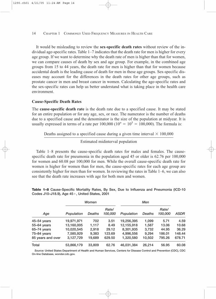
Table 1–8 presents the cause-specific death rates for males and females. The cause-specific death rate for pneumonia in the population aged 45 or older is 62.76 per 100,000for women and 60.08 per 100,000 for men. While the overall cause-specific death rate forwomen is higher for women than for men, the cause-specific rates for each age group areconsistently higher for men than for women. In reviewing the rates in Table 1–6, we can alsosee that the death rate increases with age for both men and women.


Table 1–8 Cause-Specific Mortality Rates, By Sex, Due to Influenza and Pneumonia (ICD-10Codes J10–J18.9), Age 45�, United States, 2001

Women Men

Rate/ Rate/Age Population Deaths 100,000 Population Deaths 100,000 ASDR

45–54 years 19,971,971 702 3.51 19,256,395 1,099 5.71 4.5955–64 years 13,160,005 1,117 8.49 12,155,918 1,587 13.06 10.6865–74 years 10,020,545 2,918 29.12 8,301,935 3,732 44.95 36.2975–84 years 7,585,929 9,383 123.69 4,996,556 9,294 186.01 148.4485 years and over 3,127,729 19,689 629.50 1,320,580 10,502 795.26 678.71

Total 53,866,179 33,809 62.76 46,031,384 26,214 56.95 60.08


1290.ch01 4/21/05 11:24 AM

Case Fatality Rate

The case fatality rate or killing power of a disease measures the probability of death amongthe diagnosed cases of a disease. The higher the ratio, the more virulent the infection. It ismost often used as a measure in acute infectious disease. The case fatality rate is not usefulin chronic disease because such diseases have a longer and more variable course.

The formula for the case-fatality rate is:

No. of deaths due to a disease during a given time interval � 100

No. of cases of the disease in the same time interval

Proportionate Mortality Ratio

The proportionate mortality ratio (PMR) describes the proportion of all deaths for agiven time interval that are due to a specific cause. Each cause is expressed as a percent-age of all deaths, and the sum of all the causes is 1.00 (100%). The PMR is not a mortal-ity rate, since the denominator is all deaths, not the population in which the deathsoccurred. Its formula is:

No. of deaths due to a disease during a given time interval � 100

No. of deaths from all causes in the same time interval

The PMR is often used to make comparisons between and within age groups and occu-pational groups, as well as for the general population. The PMR for pneumonia appears inTable 1–9.

Maternal Mortality Rate

The maternal mortality rate measures deaths associated with pregnancy. Pregnancy oftenplaces a woman at risk for medical problems that would not usually be encountered in thenonpregnant state, such as hemorrhage or toxemia of pregnancy. Pregnancy also compli-cates chronic conditions such as diabetes mellitus and heart disease. In some women, preg-nancy precipitates gestational diabetes. The maternal mortality rate is calculated only fordeaths that are related to pregnancy; thus, if a pregnant woman is killed in an automobileaccident, the death is not considered a pregnancy-related death.

The numerator is the number of deaths assigned to causes related to pregnancy during agiven time period; the denominator is the number of live births reported during the same pe-riod. Because the maternal mortality rate is usually very small, it is usually expressed as thenumber of deaths per 100,000 live births.


1290.ch01 4/21/05 11:24 AM

Rates of Infant Mortality

There are three rates of infant mortality, all of which are based on age. Of the three, the in-fant mortality rate is the most commonly used measure for comparing health status betweennations. All three rates are expressed in terms of the number of deaths per 1,000.

Neonatal Mortality Rate

The neonatal period is defined as the period from birth up to but not including 28 days ofage. The numerator is the number of deaths of infants under 28 days of age during a giventime period; the denominator is the total number of live births reported during the same pe-riod. The neonatal mortality rate may be used as an indirect measure of the quality of pre-natal care and/or the mother’s prenatal behavior (e.g., tobacco, alcohol, and drug use).

Postneonatal Mortality Rate

The postneonatal period is the time period from 28 days of age up to but not including oneyear of age. The numerator is the number of deaths among children from age 28 days up tobut not including one year of age during a given time period; the denominator is the totalnumber of live births reported less the number of neonatal deaths during the same period.The postneonatal mortality rate is often used as an indicator of the quality of the infant’shome environment.


Table 1–9 Proportionate Mortality Ratios for Influenza and Pneumonia (ICD-10 CodesJ10–J18.9), United States, 2001

Influenza andAge Pneumonia Deaths Total Deaths PMR/100

0–4 years 411 32,675 1.265–9 years 46 3,093 1.4910–14 years 46 4,002 1.1515–19 years 66 13,555 0.4920–24 years 115 18,697 0.6225–34 years 339 41,683 0.8135–44 years 983 91,674 1.0745–54 years 1,801 168,065 1.0755–64 years 2,704 244,139 1.1165–74 years 6,650 430,960 1.5475–84 years 18,677 701,929 2.6685 years and over 30,191 665,531 4.54

Total 62,029 2,416,003 2.57

Source: United States Department of Health and Human Services, Centers for Disease Control and Preven-tion (CDC), CDC On-line Database, wonder.cdc.gov.

1290.ch01 4/21/05 11:24 AM

Infant Mortality Rate

In effect, the infant mortality rate is a summary of the neonatal and postneonatal mortal-ity rates. The numerator is the number of deaths among children under one year of age; thedenominator is the number of live births reported during the same period. Table 1–10 pro-vides a summary of these rates.


Table 1–10 Frequently Used Mortality Measures

Measure Numerator (x) Denominator 10n

Crude death rate Total no. of deaths Estimated midinterval 1,000 or 10,000reported during given populationtime interval

Cause-specific death Total no. of deaths due Estimated midinterval 100,000rate to a specific cause population

during a given time interval

Proportionate Total no. of deaths due to Total no. of deaths from 100 or 1,000mortality ratio a specific cause during a all causes during the

given time interval same time interval

Case fatality rate Total no. of deaths Total no. of cases of 100assigned to a specific the disease during thedisease during a given same time intervaltime interval

Neonatal mortality No. of deaths under 28 No. of live births 1,000rate days of age during a during the same time

given time interval interval

Postneonatal rate No. of deaths from 28 No. of live births 1,000days up to and not during the same timeincluding one year of interval less neonatalage, during a given time deaths interval

Infant mortality rate No. of deaths under No. of live births during 1,000one year of age during the same time intervala given time interval

Maternal mortality No. of deaths assigned No. of live births during 100,000rate to pregnancy-related the same time interval

causes during a giventime interval

1290.ch01 4/21/05 11:24 AM

FREQUENTLY USED MEASURES OF MORBIDITY

Some commonly used measures to describe the presence of disease in a community or a spe-cific location, such as a nursing home, are incidence and prevalence rates. Disease can beillness, injury, or disability, and measures can be further elaborated into specific measuresof age, sex, race, or other characteristics of a particular population.

Incidence Rate

The incidence rate is the commonly used measure for comparing frequency of disease inpopulations. Populations are compared using rates instead of raw numbers because rates ad-just for differences in the size of the populations. The incidence rate expresses the proba-bility or risk of illness in a population over a period of time. The formula for calculating theincidence rate is:

Total no. of new cases of a specific disease during a given time interval � 10n

Total population at risk during the same time interval

For the incidence rate, the denominator represents the population from which the case inthe numerator arose, such as a nursing home, school, or company. For 10n, a value is se-lected so that the smallest rate calculated results in a whole number.

Prevalence Rate

The prevalence rate is the proportion of persons in a population that have a particular dis-ease at a specific point in time, or over a specified period of time. The formula for calcu-lating the prevalence rate is:

All new and preexisting cases of a specific disease during a given time interval � 10n

Total population during the same time period

Incidence and prevalence rates are often confused. The rates differ based on which casesare included in the numerator. The numerator of the incidence rate is new cases occurringduring a given time period; the numerator of the prevalence rate is all cases present duringa given time period. In comparing the two, you can see that the incidence rate includes onlyindividuals whose illness began during a specified period of time, whereas the numeratorfor the prevalence rate includes all individuals ill from a specified cause, regardless of whenthe illness began. A case is counted in prevalence until the individual recovers. Exhibit 1–6presents an example of incidence and prevalence rates in a nursing home.

At times we may be interested in tracking prevalence rates more closely—for example,tracking Klebsiella pneumoniae on a daily basis. We can do this by calculating the point


1290.ch01 4/21/05 11:24 AM

prevalence rate. The point prevalence rate is the number of cases of a specific disease at aspecific point in time. The point prevalence rate is more narrow in its time frame than thegeneral prevalence rate. Table 1–11 displays the point prevalence rates for each day duringone week in January.

For a summary of morbidity measures, see Table 1–12.

Frequently Used Measures of Morbidity 19

Exhibit 1–6 Calculation of Incidence and Prevalence Rates of Klebsiella pneumoniae at the Manor NursingHome, Month of January

At Manor Nursing Home, 10 new cases of Klebsiella pneumoniae occurred in January. For the month ofJanuary there were a total of 17 cases of Klebsiella pneumoniae. The facility had 250 residents duringJanuary.

What are the incidence and prevalence rates for Klebsiella pneumoniae during January?

Incidence Rate

1. Identify the variable of interest (numerator) and population at risk (denominator).Numerator: Total no. of new cases of Klebsiella pneumoniae in January Denominator: Total no. of nursing home residents in January



4. Divide the numerator by the denominator and multiply by 100 (10n � 102).(10/250) � 100 � 0.04 � 4.0%

The incidence rate for Klebsiella pneumoniae for the month of January is 4.0%.

Prevalence Rate

1. Identify the variable of interest (numerator) and population at risk (denominator).Numerator: Total no. of cases of Klebsiella pneumoniae in January Denominator: Total no. of nursing home residents in January



4. Divide the numerator by the denominator and multiply by 100 (10n � 102). (17/250) � 100 � 0.068%

The prevalence rate for Klebsiella pneumoniae for the month of January is 6.8%.

1290.ch01 4/21/05 11:24 AM

RELATIVE MEASURES OF DISEASE FREQUENCY

Risk Ratio/Relative Risk

Relative risk (RR) is a ratio that compares the risk of disease or other health event betweentwo groups. What we are comparing is the actual risk of illness between the two groups. Incalculating relative risk, we are using the actual rates of illness for each group to make thecomparison. The two groups may be differentiated by demographic variables, such as sex orrace, or by exposure to a suspected risk factor.

The group of primary interest is labeled as the exposed group, and the comparison groupis labeled the unexposed group. The exposed group is placed in the numerator, and the un-exposed group is placed in the denominator:


Table 1–11 Point Prevalence Rates of Klebsiella pneumoniae for the Manor Nursing Home, Weekof January 3

Sun. Mon. Tues. Weds. Thurs. Fri. Sat.

No. of cases 10 12 14 13 15 16 16No. of residents 250 250 250 250 250 250 250

Point Prevalence rate 4.0% 4.8% 5.6% 5.2% 6.0% 6.4% 6.4%

Table 1–12 Frequently Used Measures of Morbidity

Measure Numerator Denominator

Basic formula for No. of events occurring during No. of cases or computing rates a given time interval population at risk during the

same time interval

Incidence rate Total no. of new cases of a Total population at risk duringspecific disease during a the same time intervalgiven time interval

Prevalence rate All new and preexisting cases Total population during theof a specific disease during same time intervala given time interval

Relative risk Risk for exposed group Risk for unexposed group

Relative risk using Incidence rate for group Incidence rate for comparisonincidence rates of primary interest group

Attributable risk Risk for exposed group minus Risk for exposed grouprisk for unexposed group

1290.ch01 4/21/05 11:24 AM

Risk for exposed group

Risk for unexposed group

A risk ratio of 1.0 indicates that the risk is identical in both groups; a risk ratio greaterthan 1.0 indicates that the risk is greater for the numerator group; and a risk ratio of less than1.0 indicates that the risk is less for the numerator group.

As an example, we can compare the risk of death due to malignancies in men versuswomen in Michigan in 2001. First, the collected data are summarized in a two-by-two table.Two-by-two refers to two variables, each with two categories, as shown in Table 1–13.

Relative Measures of Disease Frequency 21

Table 1–13 Relative Risk of Death Due to Malig-nancies, Women versus Men Aged 65�, State ofMichigan, 2001

Death Due to Pneumonia

Sex Yes No Total

Men 7,153 21,507 28,660(a) (b) (a � b)

Women 6,565 28,890 35,455(c) (d) (c � d)

Risk of illness among men:a/(a � b) � 7,153/(7,15321,507) � 0.2496

Risk of illness among womenc/(c � d) � 6,565/(6,565 � 28,890) 0.1852

Risk ratio, men to women: 0.2496/1852 � 1.34Thus, the risk of death due to malignancyamong men aged 65� is 1.3 times greaterthan the risk of death due to malignancy inwomen in the same age group.

Source: United States Department of Health and Human Ser-vices, Centers for Disease Control and Prevention (CDC), CDCOn-line Database, wonder.cdc.gov.

To determine the risk of death among men, we compare the total number of men who died from malignancies (a � 7,153) to the total number of men in the group of interest (a � b � 7,153 � 21,507). The same procedure is followed to determine the risk of deathdue to pneumonia among women. The two ratios are then compared to determine the RR ofdeath due to malignancies among men as compared to women. A summary of these calcu-lations appears in Table 1–13. Note that the RR in each group is somewhat high, 25.0% and18.5% respectively. Deaths due to malignancies were the second leading cause of death inthe state of Michigan in 2001.

Instead of using the risk ratios to compare risks between groups, we can use actual ratesto make the same comparisons. In Table 1–14, hypothetical mortality rates are used to com-

1290.ch01 4/21/05 11:24 AM

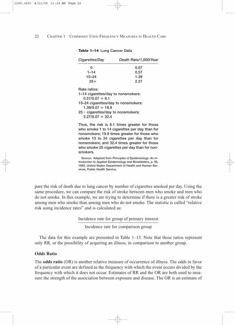
pare the risk of death due to lung cancer by number of cigarettes smoked per day. Using thesame procedure, we can compare the risk of stroke between men who smoke and men whodo not smoke. In this example, we are trying to determine if there is a greater risk of strokeamong men who smoke than among men who do not smoke. The statistic is called “relativerisk using incidence rates” and is calculated as:

Incidence rate for group of primary interest

Incidence rate for comparison group

The data for this example are presented in Table 1–15. Note that these ratios representonly RR, or the possibility of acquiring an illness, in comparison to another group.

Odds Ratio

The odds ratio (OR) is another relative measure of occurrence of illness. The odds in favorof a particular event are defined as the frequency with which the event occurs divided by thefrequency with which it does not occur. Estimates of RR and the OR are both used to mea-sure the strength of the association between exposure and disease. The OR is an estimate of


Table 1–14 Lung Cancer Data

Cigarettes/Day Death Rate/1,000/Year

0 0.071–14 0.5715–24 1.39

25� 2.27

Rate ratios:1–14 cigarettes/day to nonsmokers:

0.57/0.07 � 8.115–24 cigarettes/day to nonsmokers:

1.39/0.07 � 19.925� cigarettes/day to nonsmokers:

2.27/0.07 � 32.4

Thus, the risk is 8.1 times greater for thosewho smoke 1 to 14 cigarettes per day than fornonsmokers; 19.9 times greater for those whosmoke 15 to 24 cigarettes per day than fornonsmokers; and 32.4 times greater for thosewho smoke 25 cigarettes per day than for non-smokers.

Source: Adapted from Principles of Epidemiology: An In-troduction to Applied Epidemiology and Biostatistics, p. 95,1992, United States Department of Health and Human Ser-vices, Public Health Service.

1290.ch01 4/21/05 11:24 AM

RR. It is calculated from data obtained from retrospective studies where actual incidencerates are not calculated.

To calculate the OR, a two-by-two table is first constructed as shown in Table 1–16. Ex-hibit 1–7 displays the calculation of the odds ratio using the data from Table 1–15. The re-sults indicate that the odds of having a stroke is 1.93 times greater in men who smoke thanin men who do not smoke.


Table 1–15 Twelve-Year Risk of StrokeAmong Male Smokers and Nonsmokers

Stroke

Smokers Yes No Total

Yes 171 3,264 3,435No 117 4,320 4,437Total 288 7,584 7,872

Risk of stroke among smokers: 171/3,435 � 0.049

Risk of stroke among nonsmokers: 117/4,437 � 0.026

Risk of male smokers to male nonsmokers: 0.049/0.026 � 1.88

Thus, the risk of stroke is 1.88, or almost twotimes greater in men who smoke than menwho do not smoke.

Table 1–16 Two-by-Two Table for Odds Ratio

Disease

Risk Factor Cases Non-cases

Present a bAbsent c d

Odds Ratio � (a � d)/(b � c), where a � numberof persons with disease and with exposure ofinterest, b � number of persons without dis-ease and with exposure of interest, c � num-ber of persons with disease but withoutexposure of interest, and d � number of per-sons without disease and without exposure ofinterest.

a � c � total persons with disease (cases)b � d � total persons without disease (controls)

1290.ch01 4/21/05 11:24 AM

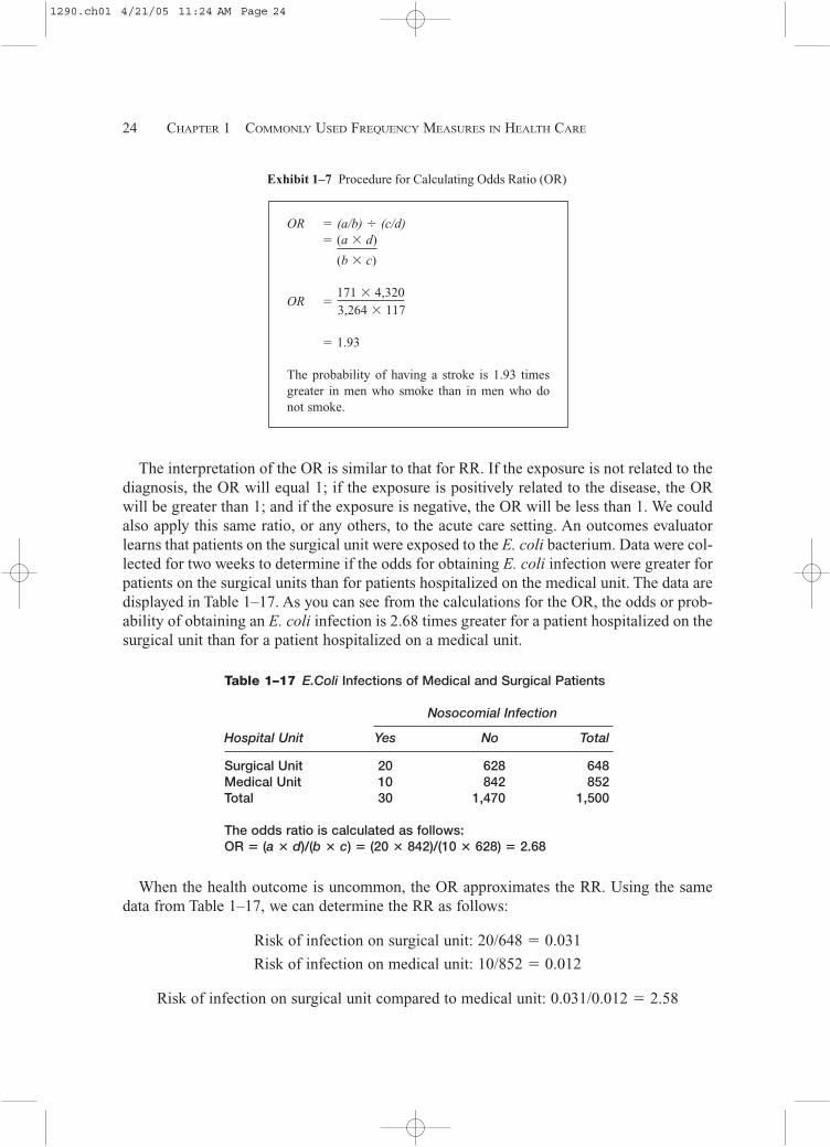
The interpretation of the OR is similar to that for RR. If the exposure is not related to thediagnosis, the OR will equal 1; if the exposure is positively related to the disease, the ORwill be greater than 1; and if the exposure is negative, the OR will be less than 1. We couldalso apply this same ratio, or any others, to the acute care setting. An outcomes evaluatorlearns that patients on the surgical unit were exposed to the E. coli bacterium. Data were col-lected for two weeks to determine if the odds for obtaining E. coli infection were greater forpatients on the surgical units than for patients hospitalized on the medical unit. The data aredisplayed in Table 1–17. As you can see from the calculations for the OR, the odds or prob-ability of obtaining an E. coli infection is 2.68 times greater for a patient hospitalized on thesurgical unit than for a patient hospitalized on a medical unit.


Exhibit 1–7 Procedure for Calculating Odds Ratio (OR)

OR � (a/b) � (c/d)� (a � d)

(b � c)

OR �171 � 4,3203,264 � 117

� 1.93

The probability of having a stroke is 1.93 timesgreater in men who smoke than in men who donot smoke.

Table 1–17 E.Coli Infections of Medical and Surgical Patients

Nosocomial Infection

Hospital Unit Yes No Total

Surgical Unit 20 628 648Medical Unit 10 842 852Total 30 1,470 1,500

The odds ratio is calculated as follows:OR � (a � d)/(b � c) � (20 � 842)/(10 � 628) � 2.68

When the health outcome is uncommon, the OR approximates the RR. Using the samedata from Table 1–17, we can determine the RR as follows:

Risk of infection on surgical unit: 20/648 � 0.031

Risk of infection on medical unit: 10/852 � 0.012

Risk of infection on surgical unit compared to medical unit: 0.031/0.012 � 2.58

1290.ch01 4/21/05 11:24 AM

As you can see, the results for both the OR and the RR are similar: 2.68 and 2.58, respectively.

Attributable Risk

The attributable risk (AR) is a measure of the impact of a disease or other causative fac-tor on a population. With this calculation, we assume that the occurrence of the disease in agroup not exposed to the risk factor represents the baseline or expected risk for that disease;any risk above that level in the exposed group is attributed to exposure to the risk factor. Ba-sically, the assumption is that the disease will occur in some individuals even without ex-posure to a given risk factor. The AR measures the additional risk of illness as a result of anindividual’s exposure to the risk factor. With AR, we attempt to answer the question, “Howmuch of the disease that occurs can be attributed to a certain exposure?” and subsequently,“How much of the risk of disease can we prevent if we eliminate the exposure to the riskfactor in question?”

(Risk for exposed group) � (risk for unexposed group) � 100

Risk for exposed group

Using the lung cancer data from Table 1–14, we calculate the attributable proportion asoutlined in Exhibit 1–8.


Exhibit 1–8 Calculation of Attributable Proportion

1. Identify the exposed group rate. Lung cancerdeath rate for smokers of 1–14 cigarettes perday � 0.57 per 1,000 per year

2. Identify the unexposed group rate.

0.07 per 1,000 per year

3. Calculate the attributable proportion.

0.57 � 0.07 � 100 � 87.7

0.57

The conclusion from the calculation of the attributable proportion is that 87.7% of thelung cancer cases are due to or attributed to smoking 1 to 14 cigarettes per day. Approxi-mately 12% (1.00 � 0.877) of the cases in this group would have occurred without expo-sure to the risk factor—in this case, cigarettes. By carrying out the calculations for theremaining two groups, we can see that the AR increases with the number of cigarettessmoked per day.

1290.ch01 4/21/05 11:24 AM

AR 15–24 cigarettes/day � [(1.39 � 0.07)/1.39] � 100 � 95.0%

AR 25� cigarettes/day � [(2.27 � 0.07)/2.27] � 100 � 96.9%

Approximately 5% and 3%, respectively, of the individuals in these two groups wouldhave acquired the disease regardless of whether or not they smoked cigarettes.

KAPLAN-MEIER SURVIVAL ANALYSIS

Many individuals within the health information management profession are employed in tu-mor registries or in the capacity of assisting researchers in analyzing data from clinical tri-als. In clinical trials, the researcher is interested in determining whether a specific medicalor surgical intervention improves survival for a particular condition. A major criterion inmeasuring the success of a clinical trial is the survival time of individuals undergoing theexperimental treatment. In survival analysis we are examining the survival rates as a resultof a clinical trial involving a medical or surgical intervention. A major problem in conduct-ing survival analysis is that patients may be lost to follow up or some may be censored. Acensored patient is one who for some reason is unable to complete the study.

There are several methods for analyzing survival rates, but we will limit the discussion tothe Kaplan Meier method, a type of life table analysis, since it is most often used in analy-sis of data collected from clinical trials. Kaplan-Meier survival analysis requires a di-chotomous outcome such as survival/death or improvement/no improvement.

The major reason for using the Kaplan Meier method is that it takes into account some ofthe problems commonly encountered when conducting prospective studies. The KaplanMeier method compensates for subjects who are lost to follow-up or who are unable to com-plete the study. To conduct an accurate survival analysis, we need to know:

• the reason for patients’ withdrawal from the study (i.e., death, loss to follow-up, or cen-sorship)

• the date of withdrawal from study (i.e., date of death, date patient last seen alive or lostto follow-up, or date withdrawn from study)

When survival time is censored, the subject is alive at the time of analysis, or was alive atthe time last seen. Survival times tagged with a “+” indicate that they are censored. Table1–18 presents some hypothetical data for 10 patients in a clinical trial for treatment of blad-der cancer. The survival times, in months (column 1), for each patient are rank ordered fromlowest to highest.

Each row in Table 1–18 represents an interval. The first row is the first study interval. Aninterval is a death-free time period. So row 1, column 6, represents a death-free time periodof less than 23 months. This is interpreted as meaning that the probability (px) of survivingup to but less than 23 months is 1.000 (10/10). The px of the first interval is always 1.000because the first death ends the first interval. The occurrence of a death ends one death-freeinterval and begins another.


1290.ch01 4/21/05 11:24 AM

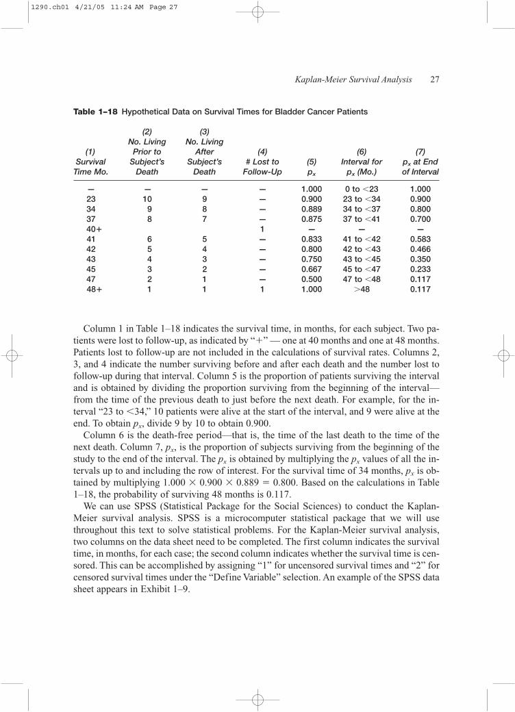
Column 1 in Table 1–18 indicates the survival time, in months, for each subject. Two pa-tients were lost to follow-up, as indicated by “�” — one at 40 months and one at 48 months.Patients lost to follow-up are not included in the calculations of survival rates. Columns 2,3, and 4 indicate the number surviving before and after each death and the number lost tofollow-up during that interval. Column 5 is the proportion of patients surviving the intervaland is obtained by dividing the proportion surviving from the beginning of the interval—from the time of the previous death to just before the next death. For example, for the in-terval “23 to �34,” 10 patients were alive at the start of the interval, and 9 were alive at theend. To obtain px, divide 9 by 10 to obtain 0.900.

Column 6 is the death-free period—that is, the time of the last death to the time of thenext death. Column 7, px, is the proportion of subjects surviving from the beginning of thestudy to the end of the interval. The px is obtained by multiplying the px values of all the in-tervals up to and including the row of interest. For the survival time of 34 months, px is ob-tained by multiplying 1.000 � 0.900 � 0.889 � 0.800. Based on the calculations in Table1–18, the probability of surviving 48 months is 0.117.

We can use SPSS (Statistical Package for the Social Sciences) to conduct the Kaplan-Meier survival analysis. SPSS is a microcomputer statistical package that we will usethroughout this text to solve statistical problems. For the Kaplan-Meier survival analysis,two columns on the data sheet need to be completed. The first column indicates the survivaltime, in months, for each case; the second column indicates whether the survival time is cen-sored. This can be accomplished by assigning “1” for uncensored survival times and “2” forcensored survival times under the “Define Variable” selection. An example of the SPSS datasheet appears in Exhibit 1–9.

Kaplan-Meier Survival Analysis 27

Table 1–18 Hypothetical Data on Survival Times for Bladder Cancer Patients

(2) (3)No. Living No. Living

(1) Prior to After (4) (6) (7)Survival Subject’s Subject’s # Lost to (5) Interval for px at End

Time Mo. Death Death Follow-Up px px (Mo.) of Interval

— — — — 1.000 0 to �23 1.00023 10 9 — 0.900 23 to �34 0.90034 9 8 — 0.889 34 to �37 0.80037 8 7 — 0.875 37 to �41 0.70040� 1 — — —41 6 5 — 0.833 41 to �42 0.58342 5 4 — 0.800 42 to �43 0.46643 4 3 — 0.750 43 to �45 0.35045 3 2 — 0.667 45 to �47 0.23347 2 1 — 0.500 47 to �48 0.11748� 1 1 1 1.000 48 0.117

1290.ch01 4/21/05 11:24 AM

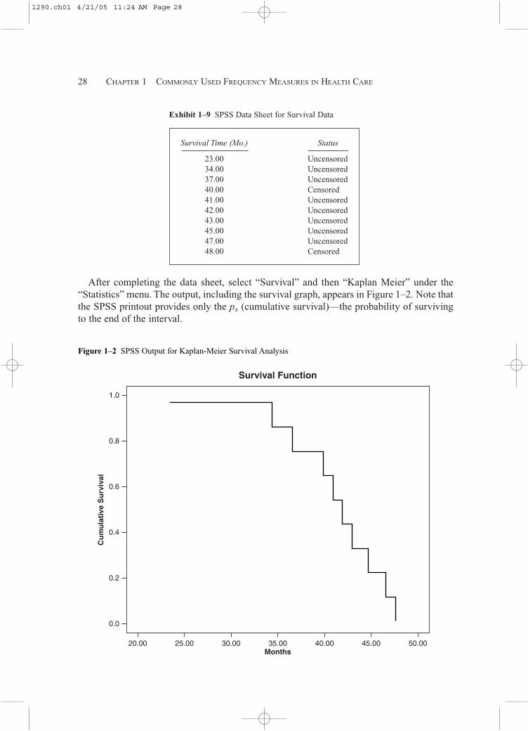
After completing the data sheet, select “Survival” and then “Kaplan Meier” under the“Statistics” menu. The output, including the survival graph, appears in Figure 1–2. Note thatthe SPSS printout provides only the px (cumulative survival)—the probability of survivingto the end of the interval.


Exhibit 1–9 SPSS Data Sheet for Survival Data

Survival Time (Mo.) Status

23.00 Uncensored34.00 Uncensored37.00 Uncensored40.00 Censored41.00 Uncensored42.00 Uncensored43.00 Uncensored45.00 Uncensored47.00 Uncensored48.00 Censored

1.0

0.8

0.6

0.4

0.2

0.0

20.00 25.00 30.00 35.00

Survival Function

40.00 45.00 50.00

Cu

mu

lati

ve S

urv

ival

Months

Figure 1–2 SPSS Output for Kaplan-Meier Survival Analysis

1290.ch01 4/21/05 11:24 AM

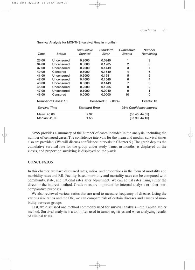
SPSS provides a summary of the number of cases included in the analysis, including thenumber of censored cases. The confidence intervals for the mean and median survival timesalso are provided. (We will discuss confidence intervals in Chapter 5.) The graph depicts thecumulative survival rate for the group under study. Time, in months, is displayed on the x-axis, and proportion surviving is displayed on the y-axis.

CONCLUSION

In this chapter, we have discussed rates, ratios, and proportions in the form of mortality andmorbidity rates and RR. Facility-based morbidity and mortality rates can be compared withcommunity, state, and national rates after adjustment. We can adjust rates using either thedirect or the indirect method. Crude rates are important for internal analysis or other non-comparative purposes.

We also reviewed various ratios that are used to measure frequency of disease. Using thevarious risk ratios and the OR, we can compare risk of certain diseases and causes of mor-bidity between groups.

Last, we discussed one method commonly used for survival analysis—the Kaplan Meiermethod. Survival analysis is a tool often used in tumor registries and when analyzing resultsof clinical trials.

Conclusion 29

Survival Analysis for MONTHS (survival time in months)

Cumulative Standard Cumulative NumberTime Status Survival Error Events Remaining

23.00 Uncensored 0.9000 0.0949 1 934.00 Uncensored 0.8000 0.1265 2 837.00 Uncensored 0.7000 0.1449 3 740.00 Censored 0.6000 0.1549 4 641.00 Uncensored 0.5000 0.1581 5 542.00 Uncensored 0.4000 0.1549 6 443.00 Uncensored 0.3000 0.1449 7 345.00 Uncensored 0.2000 0.1265 8 247.00 Uncensored 0.1000 0.0949 9 148.00 Censored 0.0000 0.0000 10 0

Number of Cases: 10 Censored: 0 (.00%) Events: 10

Survival Time Standard Error 95% Confidence Interval

Mean: 40.00 2.32 (35.45, 44.55)Median: 41.00 1.58 (37.90, 44.10)

1290.ch01 4/21/05 11:24 AM

ADDITIONAL RESOURCES

Gail, M.H. and Benichou, J., eds. 2000. Encyclopedia of epidemiologic methods. Wiley Reference Series in Biostatistics.Hoboken, NJ: Wiley Publishers.

Gordis, L. 1996. Epidemiology. Philadelphia: W.B. Saunders.

Jekel, J.F., et al. 1996. Epidemiology, biostatistics and preventive medicine. Philadelphia: W.B. Saunders.

Morton, R., et al. 1989. A study guide to epidemiology and biostatistics. Gaithersburg, MD: Aspen Publishers, Inc.

Anderson, K.N., Anderson, L.E., and Glanze, W.D. Mosby’s medical, nursing, and allied health dictionary. 4th ed. 1994. St. Louis, MO: C.V. Mosby.

Norman, G.R., and Streiner, D.L. 2000. Biostatistics: The bare essentials. Ontario, Canada: Hamilton.

Ohio Department of Health. 1996. Prevention Monthly 19, no. 3:6.

Pagano, M., and Gauvreau, K. 2000. Principles of biostatistics. Pacific Grove, CA: Brooks Cole Publishing.

Ratelle, S. 2001. Preventive medicine and public health: PreTest self-assessment and review. New York: McGraw-Hill/Appleton & Lange McGraw-Hill.

U.S. Department of Health and Human Services (US DHHS), Public Health Service. 1992. Principles of epidemiology: An in-troduction to applied epidemiology and biostatistics.

U.S. Department of Health and Human Services, Centers for Disease Control and Prevention (CDC), National Center forHealth Statistics (NCHS), Office of Analysis, Epidemiology, and Health Promotion (OAEHP), Compressed Mortality File(CMF) compiled from CMF 1968–1988 Series 20, No. 2A 2000, CMF 1989–1998, Series 20, No. 2E 2003 and CMF1999–2001, Series 20, No. 2G 2004 on CDC WONDER on-line database. wonder.cdc.gov.

U.S. Department of Health and Human Services, Centers for Disease Control and Prevention, National Center for HIV, STD,and TB Prevention, Division of HIV/AIDS Prevention, AIDS Public Information Data Sets, CDC WONDER on-line database. wonder.cdc.gov.

Utah Inpatient Hospital Discharge Data Set. http://hlunix.ex.state.ut.us/had.


1290.ch01 4/21/05 11:24 AM

31

Appendix 1–A

Exercises for Solving Problems

KNOWLEDGE QUESTIONS

1. Define the key terms listed at the beginning of this chapter.

2. Describe the differences and similarities between rates, ratios, and proportions.

3. Outline the procedure for age-adjusting crude mortality rates by the direct standardiza-tion method.

4. Describe the differences between the direct and indirect standardization methods of ad-justing mortality and morbidity rates.

5. Describe the differences between neonatal mortality rate, postneonatal mortality rate,and infant mortality rate.

6. Describe the difference between incidence and prevalence rates.

MULTIPLE CHOICE

For questions 1 and 2, refer to the following table:

Age Group Population No. of Deaths

� 30 15,000 2030–65 17,000 55

65 6,000 155

1. What is the crude mortality rate? a. 230b. 6.1 per 1,000c. 8.6 per 1,000 d. 6.1 per 10,000

1290.ch01 4/21/05 11:24 AM

2. The age-specific death rate for the over-65 age group is: a. 155b. 25.8 per 1,000c. 1.55 per 10,000 d. 25.8 per 10,000

PROBLEMS

1. Review the hypothetical data on deaths in the MICU in Table 1–A–1 and answer thequestions that follow: a. What is the ratio of male deaths to female deaths?b. What proportion of the patients who died were admitted from the Emergency De-

partment? What proportion were transfers from other hospitals?c. The total number of patients discharged from DRG 475 was 61. What is the case fa-

tality rate for DRG 475? d. The total number of patients discharged from DRG 483 was 51. What is the case fa-

tality rate for DRG 483? e. What is the relative risk of death for patients discharged from DRG 475 compared to

discharges from DRG 483?


Table 1–A–1 Critical Care Hospital, Deaths in the MICU by DRG

Adm.DRG DRG Title Source Gender LOS

001 Craniotomy Age 17 W Cc SNF Male 2014 Intracranial Hemorrhage & Stroke W Infarct Other Male 3014 Intracranial Hemorrhage & Stroke W Infarct Emerdept Female 3020 Nervous System Infection Except Viral Meningitis Other Female 15075 Major Chest Procedures Hospital Male 6105 Cardiac Valve & Oth Major Cardiothoracic Hospital Female 23

Proc W/O Card Cath123 Circulatory Disorders W Ami, Expired Hospital Male 7123 Circulatory Disorders W Ami, Expired Other Male 1123 Circulatory Disorders W Ami, Expired Other Male 4123 Circulatory Disorders W Ami, Expired Emerdept Male 5172 Digestive Malignancy W Cc Emerdept Male 1172 Digestive Malignancy W Cc Physician Male 1188 Other Digestive System Diagnoses Age 17 W Cc SNF Female 1191 Pancreas, Liver & Shunt Procedures W Cc Hospital Male 9202 Cirrhosis & Alcoholic Hepatitis Physician Female 15202 Cirrhosis & Alcoholic Hepatitis Other Male 1202 Cirrhosis & Alcoholic Hepatitis Emerdept Male 24

1290.ch01 4/21/05 11:24 AM

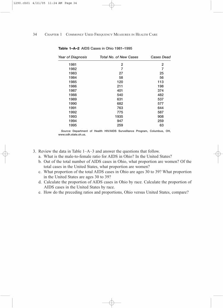
2. Review the data in Table 1–A–2 and answer the questions that follow.a. What is the case fatality rate for AIDS for the years 1981 through 1995?b. The midyear population for the state of Ohio in 1994 was 11,140,950. What is the in-

cidence rate for AIDS for 1994?

Problems 33

continuedAdm

DRG DRG Title Source Gender LOS

205 Disorders Of Liver Except Malig,Cirr,Alc Hepa W Cc Physician Male 20331 Other Kidney & Urinary Tract Diagnoses Age 17 W Cc Physician Male 44357 Uterine & Adnexa Proc For Ovarian Or Physician Female 24

Adnexal Malignancy416 Septicemia Age 17 Hospital Female 4416 Septicemia Age 17 Other Male 2449 Poisoning & Toxic Effects Of Drugs Age 17 W Cc Other Male 1473 Acute Leukemia W/O Major O.R. Procedure Age 17 Physician Male 5475 Respiratory System Diagnosis With Ventilator Support Physician Male 25475 Respiratory System Diagnosis With Ventilator Support Physician Female 1475 Respiratory System Diagnosis With Ventilator Support Hospital Female 1475 Respiratory System Diagnosis With Ventilator Support Other Female 1475 Respiratory System Diagnosis With Ventilator Support Hospital Female 21475 Respiratory System Diagnosis With Ventilator Support Other Male 5475 Respiratory System Diagnosis With Ventilator Support Hospital Female 8475 Respiratory System Diagnosis With Ventilator Support Emerdept Female 10475 Respiratory System Diagnosis With Ventilator Support Clinic Male 13475 Respiratory System Diagnosis With Ventilator Support SNF Female 1475 Respiratory System Diagnosis With Ventilator Support Emerdept Male 5475 Respiratory System Diagnosis With Ventilator Support Clinic Female 4475 Respiratory System Diagnosis With Ventilator Support Emerdept Male 3475 Respiratory System Diagnosis With Ventilator Support Other Female 12475 Respiratory System Diagnosis With Ventilator Support Other Female 5483 Trac W Mech Vent 96�Hrs Or Pdx Except Face, Hospital Female 30

Mouth & Neck Dx 483 Trac W Mech Vent 96�Hrs Or Pdx Except Face, Hospital Male 19

Mouth & Neck Dx 483 Trac W Mech Vent 96�Hrs Or Pdx Except Face, Hospital Male 22

Mouth & Neck Dx 483 Trac W Mech Vent 96�Hrs Or Pdx Except Face, Physician Female 46

Mouth & Neck Dx 483 Trac W Mech Vent 96�Hrs Or Pdx Except Face, Other Female 28

Mouth & Neck Dx

1290.ch01 4/21/05 11:24 AM

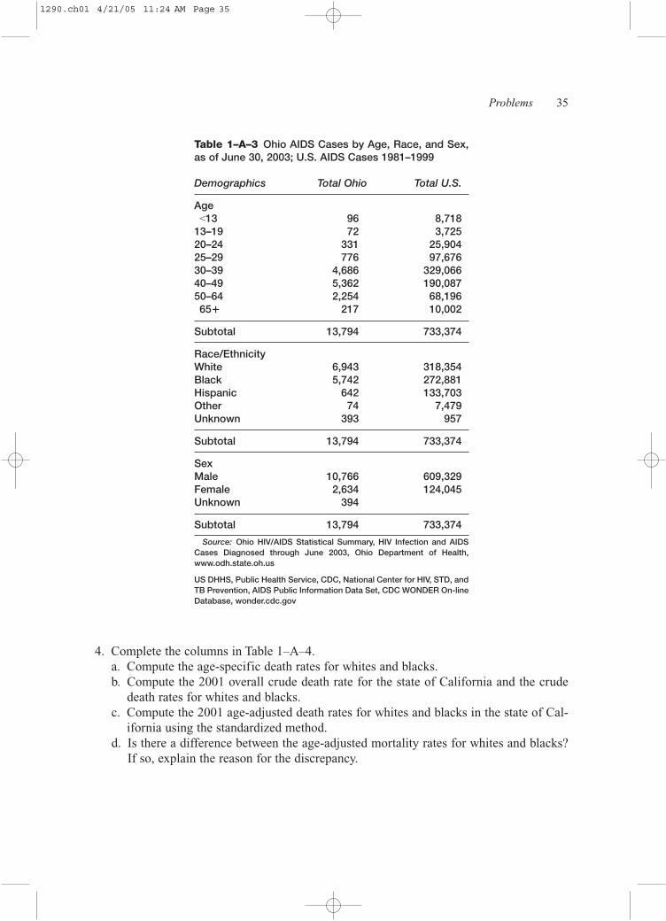
3. Review the data in Table 1–A–3 and answer the questions that follow.a. What is the male-to-female ratio for AIDS in Ohio? In the United States?b. Out of the total number of AIDS cases in Ohio, what proportion are women? Of the

total cases in the United States, what proportion are women? c. What proportion of the total AIDS cases in Ohio are ages 30 to 39? What proportion

in the United States are ages 30 to 39? d. Calculate the proportion of AIDS cases in Ohio by race. Calculate the proportion of

AIDS cases in the United States by race. e. How do the preceding ratios and proportions, Ohio versus United States, compare?


Table 1–A–2 AIDS Cases in Ohio 1981–1995

Year of Diagnosis Total No. of New Cases Cases Dead

1981 2 21982 7 71983 27 251984 58 561985 120 1131986 211 1981987 401 3741988 540 4821989 631 5371990 682 5771991 763 6441992 775 5871993 1935 9081994 947 2591995 259 63

Source: Department of Health HIV/AIDS Surveillance Program, Columbus, OH,www.odh.state.oh.us.

1290.ch01 4/21/05 11:24 AM

4. Complete the columns in Table 1–A–4.a. Compute the age-specific death rates for whites and blacks.b. Compute the 2001 overall crude death rate for the state of California and the crude

death rates for whites and blacks. c. Compute the 2001 age-adjusted death rates for whites and blacks in the state of Cal-

ifornia using the standardized method. d. Is there a difference between the age-adjusted mortality rates for whites and blacks?

If so, explain the reason for the discrepancy.

Problems 35

Table 1–A–3 Ohio AIDS Cases by Age, Race, and Sex,as of June 30, 2003; U.S. AIDS Cases 1981–1999

Demographics Total Ohio Total U.S.

Age<13 96 8,718

13–19 72 3,72520–24 331 25,90425–29 776 97,67630–39 4,686 329,06640–49 5,362 190,08750–64 2,254 68,19665� 217 10,002

Subtotal 13,794 733,374

Race/EthnicityWhite 6,943 318,354Black 5,742 272,881Hispanic 642 133,703Other 74 7,479Unknown 393 957

Subtotal 13,794 733,374

SexMale 10,766 609,329Female 2,634 124,045Unknown 394

Subtotal 13,794 733,374

Source: Ohio HIV/AIDS Statistical Summary, HIV Infection and AIDSCases Diagnosed through June 2003, Ohio Department of Health,www.odh.state.oh.us

US DHHS, Public Health Service, CDC, National Center for HIV, STD, andTB Prevention, AIDS Public Information Data Set, CDC WONDER On-lineDatabase, wonder.cdc.gov

1290.ch01 4/21/05 11:24 AM

5. Calculate the odds ratio for the data in Table 1–13. Interpret the results.

6. At Critical Care Hospital, the complication rate for hip replacement surgery is 8.96%.The relevant statistics appear in Table 1–A–5. The administrative staff at the hospital isconcerned that the hospital complication rate does not compare favorably with the over-all complication rate of all patients with hip replacement surgery in the county. The com-plication rate for the county is 5.5%. The county complication rate for patients age 65 orolder is 8.0%; for those under age 65, the complication rate is 3.0%. Using the indirectmethod of standardization, calculate the complication rate for the hospital that has beenadjusted for age.


Table 1–A–4 Age-Specific Mortality Rates, State of California, 2001

(h) (i)Expected Expected

(g) No. of No. of(c) (d) (f) Comb. Deaths Deaths

(a) (b) White Black (e) Black Pop. Whites BlacksAge White Pop. Deaths ASDR Pop. Deaths ASDR Total (g � c) (g � f)

�1 428,238 2,131 33,774 435 462,0121–4 1,565,447 413 170,587 80 1,736,0345–9 2,120,923 291 240,189 45 2,361,112

10–14 2,084,668 311 244,031 55 2,328,69915–19 1,929,503 1,129 208,006 185 2,137,50920–24 1,916,977 1,569 186,458 274 2,103,43525–34 4,123,447 3,399 373,455 644 4,496,90235–44 4,318,242 7,394 415,178 1,258 4,733,42045–54 3,554,132 13,766 304,914 2,339 3,859,04655–64 2,201,539 18,939 176,743 2,647 2,378,28265–74 1,531,032 33,192 11,657 3,517 1,542,68975–84 1,119,160 59,115 62,592 3,998 1,181,75285� 395,512 57,200 20,542 2,906 416,054

Total 27,288,820 198,849 2,448,126 18,383 29,736,946


Table 1–A–5 Critical Care Hospital, Hip Replacement Surgery

No. of Patients with ComplicationAge Group No. of Patients Complications Rate

� 65 170 17 10.00%� 65 42 2 4.76%

Total 212 19 8.96%

1290.ch01 4/21/05 11:24 AM

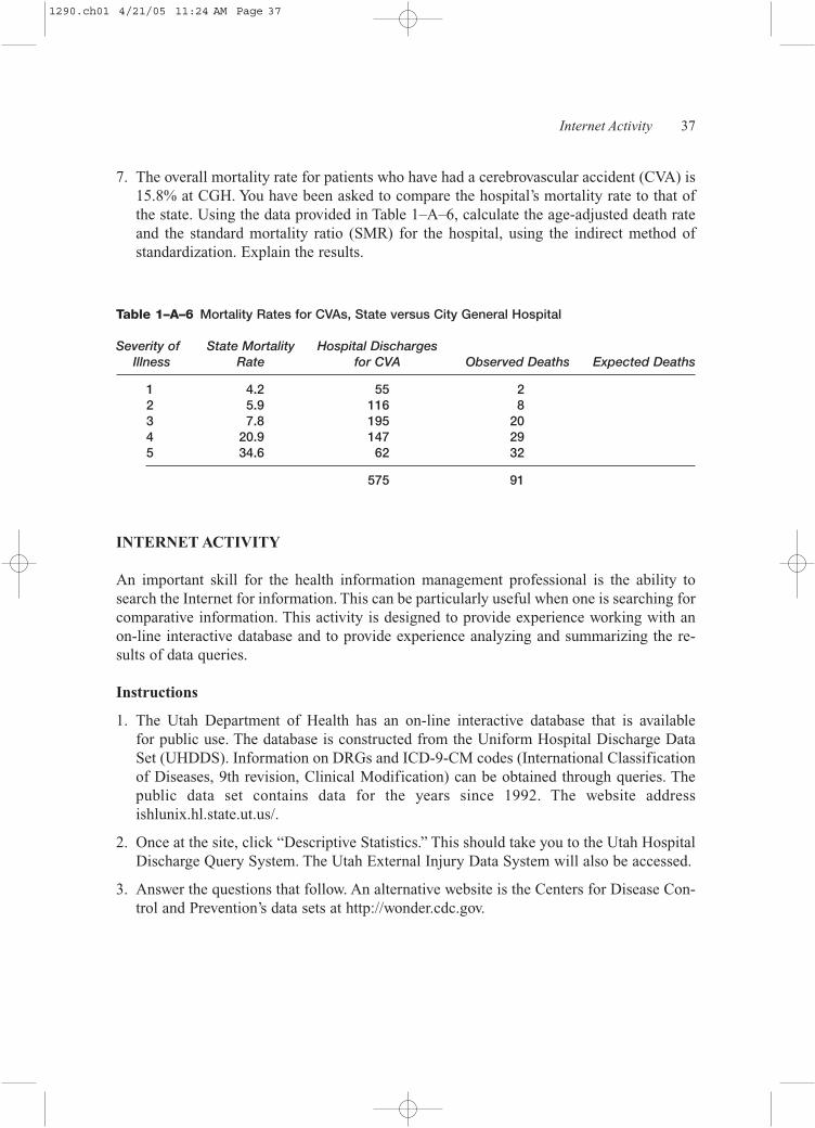
7. The overall mortality rate for patients who have had a cerebrovascular accident (CVA) is15.8% at CGH. You have been asked to compare the hospital’s mortality rate to that ofthe state. Using the data provided in Table 1–A–6, calculate the age-adjusted death rateand the standard mortality ratio (SMR) for the hospital, using the indirect method ofstandardization. Explain the results.

Internet Activity 37

Table 1–A–6 Mortality Rates for CVAs, State versus City General Hospital

Severity of State Mortality Hospital Discharges Illness Rate for CVA Observed Deaths Expected Deaths

1 4.2 55 22 5.9 116 83 7.8 195 204 20.9 147 295 34.6 62 32

575 91

INTERNET ACTIVITY

An important skill for the health information management professional is the ability tosearch the Internet for information. This can be particularly useful when one is searching forcomparative information. This activity is designed to provide experience working with anon-line interactive database and to provide experience analyzing and summarizing the re-sults of data queries.

Instructions

1. The Utah Department of Health has an on-line interactive database that is available for public use. The database is constructed from the Uniform Hospital Discharge DataSet (UHDDS). Information on DRGs and ICD-9-CM codes (International Classificationof Diseases, 9th revision, Clinical Modification) can be obtained through queries. Thepublic data set contains data for the years since 1992. The website addressishlunix.hl.state.ut.us/.

2. Once at the site, click “Descriptive Statistics.” This should take you to the Utah HospitalDischarge Query System. The Utah External Injury Data System will also be accessed.

3. Answer the questions that follow. An alternative website is the Centers for Disease Con-trol and Prevention’s data sets at http://wonder.cdc.gov.

1290.ch01 4/21/05 11:24 AM

Questions

1. For the diagnosis of acute myocardial infarction, ICD-9-CM category 410:a. Prepare a bar graph that displays the number of deaths due to AMI by year, 1998

through 2002.b. Prepare a line graph that displays the number of deaths by gender for the years 1998

through 2002. What are your conclusions?c. Prepare a table that displays the number of deaths due to AMI by age group. Use the

table to prepare a bar graph of the same information. d. Prepare a bar graph that displays the average length of stay by gender for the years

1992 through 2002. What are your conclusions after reviewing the data?e. Prepare a line graph that displays the median charges by year, 1992 through 2002.

What does the graph indicate?

2. How many patients with coronary atherosclerosis, ICD-9-CM category 414, had a coro-nary artery bypass graft (CABG) procedure, ICD-9-CM procedure category 36?a. Prepare a line graph that displays both the total number of discharges with a principal

diagnosis of coronary atherosclerosis and the total number with the CABG procedure.b. Construct a bar graph that displays average length of stay, by year and gender, for pa-

tients with coronary atherosclerosis and CABG procedure for the years 1998–2002. c. Construct a bar graph that displays the number of CABG procedures, by gender, for

the years 1998–2002. What are your conclusions?

3. Determine the number of patient discharges with pathological fractures, ICD-9-CM code733.1, by year, 1998 through 2002, and by gender. You are interested in patients aged 65years and over. Prepare a line graph displaying the number of discharges by year and bygender. Discuss your findings.

4. In table form, how many patients were discharged, by year, 1998 through 2002, and bygender, with malignant neoplasms of the trachea, bronchus, and lung? Use the selectionoption that is available on the database. Prepare a bar or line graph that displays the per-centage of patients, by gender, who expired from these illnesses.

5. For ICD-9-CM code 185, for the years 1998 through 2002:a. Prepare a bar graph or pie chart, by third-party payer, of men, aged 45 and older, dis-

charged with a diagnosis of prostate cancer.b. Prepare a bar graph that displays the number of men, by age group, discharged with

prostate cancer.c. Discuss your findings.

6. For patients discharged with pneumonia during the years 1998 through 2002 (use the se-lection option that is available on the database):a. Prepare a table that reports the average length of stay for patients discharged with pneu-

monia by year and by gender. Include only patients who are aged 65 years and older.b. Prepare a bar or line graph to display your results. c. Discuss your findings.


1290.ch01 4/21/05 11:24 AM

commonly used frequency measures in health care used frequency measures in health care 1 ......

Documents