COMMON PROBABILITY DISTRIBUTIONS AND THEIR

USES

Learning Objectives

• Have a broad understanding of how probability distributions are used in improvement projects.

• Review the origin and use of common probability distributions.

How does it help?

Probability distributions are necessary to:

•determine whether an event is significant or due to random chance.

•predict the probability of specific performance given historical characteristics.

Probability distributions are necessary to:

•determine whether an event is significant or due to random chance.

•predict the probability of specific performance given historical characteristics.

IMPROVEMENT ROADMAPUses of Probability Distributions

BreakthroughStrategy

Characterization

Phase 1:Measurement

Phase 2:

Analysis

Optimization

Phase 3:Improvement

Phase 4:

Control

•Baselining Processes

•Verifying Improvements

Common Uses

Focus on understanding the use of the distributions

Practice with examples wherever possible

Focus on the use and context of the tool

KEYS TO SUCCESS

X

X X X

X

Data points vary, but as the data accumulates, it forms a distribution which occurs naturally.

Location Spread Shape

Distributions can vary in:

PROBABILITY DISTRIBUTIONS, WHERE DO THEY COME FROM?

-4

-3

-2

-1

0

1

2

3

4

0 1 2 3 4 5 6 7

-4

-3

-2

-1

0

1

2

3

4

0 1 2 3 4 5 6 7

0

1

2

3

4

0 1 2 3 4 5 6 7

Original Population

Subgroup Average

Subgroup Variance (s2)

Continuous Distribution

Normal Distribution

χ2 Distribution

COMMON PROBABILITY DISTRIBUTIONS

THE LANGUAGE OF MATHSymbol Name Statistic M eaning Common Uses

α Alpha Significance level Hypothesis Testing,DOE

χ2 Chi Square Probability Distribution Confidence Intervals, ContingencyTables, Hypothesis Testing

Σ Sum Sum of Individual values Variance Calculations

t t, Student t Probability Distribution Hypothesis Testing, Confidence Intervalof the Mean

n SampleSize

Total size of the SampleTaken

Nearly all Functions

ν Nu Degree of Freedom Probability Distributions, HypothesisTesting, DOE

β Beta Beta Risk Sample Size Determination

δ Delta Difference betweenpopulation means

Sample Size Determination

Ζ SigmaValue

Number of StandardDeviations a value Existsfrom the Mean

Probability Distributions, ProcessCapability, Sample Size Determinations

Population and Sample Symbology

Value Population Sample

Mean μ

Variance σ2 s2

Standard Deviation σ s

Process Capability Cp

Binomial Mean

x

P P

Cp

THREE PROBABILITY DISTRIBUTIONS

tX

sn

CALC =− μ

Significant t tCALC CRIT= ≥

Significant F FCALC CRIT= ≥F sscalc = 1

2

22

( )χα ,df

e a

e

f f

f2

2

=−

Significant CALC CRIT= ≥χ χ2 2

Note that in each case, a limit has been established to determine what is random chance verses significant difference. This point is called the critical value. If the calculated value exceeds this critical value, there is very low probability (P<.05) that this is due to random chance.

-1σ-1σ +1σ+1σ

68.26%

+/- 1σ = 68%2 tail = 32%

1 tail = 16%

-2σ-2σ +2σ+2σ

95.46%

+/- 2σ = 95%

2 tail = 4.6%

1 tail = 2.3%

-3σ-3σ +3σ+3σ

99.73%

+/- 3σ = 99.7%

2 tail = 0.3%

1 tail = .15%

Common Test Values

Z(1.6) = 5.5% (1 tail α=.05)

Z(2.0) = 2.5% (2 tail α=.05)

Common Test Values

Z(1.6) = 5.5% (1 tail α=.05)

Z(2.0) = 2.5% (2 tail α=.05)

Z TRANSFORM

The Focus of Six Sigma…..

Y = f(x)

All critical characteristics (Y) are driven by factors (x) which are “downstream” from the results….

Attempting to manage results (Y) only causes increased costs due to rework, test and inspection…

Understanding and controlling the causative factors (x) is the real key to high quality at low cost...Probability distributions identify sources of

causative factors (x). These can be identified and verified by testing which shows their significant effects against the backdrop of random noise.

Probability distributions identify sources of causative factors (x). These can be identified and verified by testing which shows their significant effects against the backdrop of random noise.

BUT WHAT DISTRIBUTION SHOULD I USE?

Characterize Population

Characterize Population

Population Average

Population Variance

Determine Confidence Interval for

Point Values

•F Stat (n>30)

•F’ Stat (n<10)

• χ2 Stat (n>5)

•Z Stat (n>30)

•Z Stat (p)

•t Stat (n<30)

• τ Stat (n<10)

•Z Stat (n>30)

•Z Stat (p)

•t Stat (n<30)

• τ Stat (n<10)

•F Stat (n>30)

• χ2 Stat (n>5)

•Z Stat (μ,n>30)

•Z Stat (p)

•t Stat (μ,n<30)

• χ2 Stat (σ,n<10)

• χ2 Stat (Cp)

Compare 2 Population Averages

Compare a Population Average Against a

Target Value

Compare 2 Population Variances

Compare a Population Variance

Against Target Value(s)

HOW DO POPULATIONS INTERACT?

These interactions form a new population which can now be used to predict future performance.

HOW DO POPULATIONS INTERACT?ADDING TWO POPULATIONS

Population means interact in a simple intuitive manner.

μ1 μ2

Means Add

μ1 + μ2 = μnew

Population dispersions interact in an additive manner

σ1 σ2

Variations Add

σ12 + σ2

2 = σnew2

σnew

μnew

HOW DO POPULATIONS INTERACT?SUBTRACTING TWO POPULATIONS

Population means interact in a simple intuitive manner.

μ1 μ2

Means Subtract

μ1 - μ2 = μnew

Population dispersions interact in an additive manner

σ1 σ2

Variations Add

σ12 + σ2

2 = σnew2

σnew

μnew

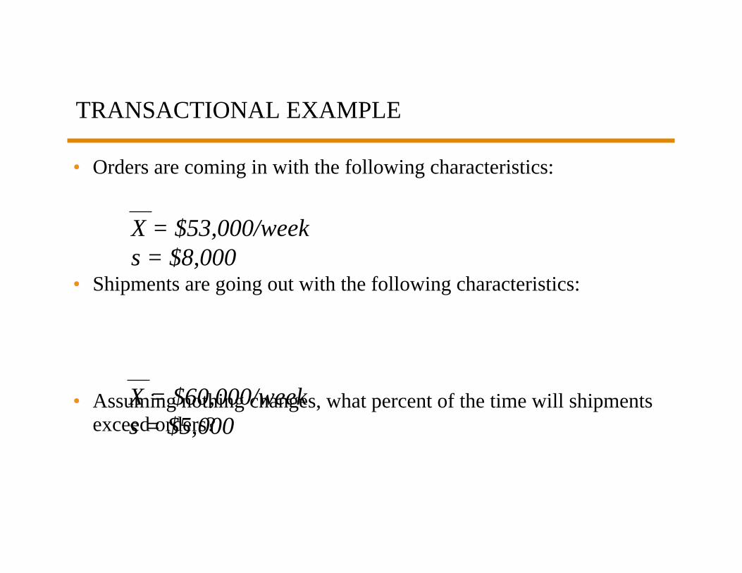
TRANSACTIONAL EXAMPLE

• Orders are coming in with the following characteristics:

• Shipments are going out with the following characteristics:

• Assuming nothing changes, what percent of the time will shipments exceed orders?

X = $53,000/weeks = $8,000

X = $60,000/weeks = $5,000

To solve this problem, we must create a new distribution to model the situation posed in the problem. Since we are looking for shipments to exceed orders, the resulting distribution is created as follows:

X X Xshipments orders shipments orders− = − = − =$60 , $53 , $7 ,000 000 000

( ) ( )s s sshipments orders shipments orders− = + = + =2 2 2 25000 8000 $9434

The new distribution looks like this with a mean of $7000 and a standard deviation of $9434. This distribution represents the occurrences of shipments exceeding orders. To answer the original question (shipments>orders) we look for $0 on this new distribution. Anyoccurrence to the right of this point will represent shipments > orders. So, we need to calculate the percent of the curve that exists to the right of $0.

$7000

$0Shipments > orders

X = $53,000 in orders/weeks = $8,000

X = $60,000 shipped/weeks = $5,000

Orders Shipments

TRANSACTIONAL EXAMPLE

TRANSACTIONAL EXAMPLE, CONTINUED

X X Xshipments orders shipments orders− = − = − =$60 , $53 , $7 ,000 000 000

( ) ( )s s sshipments orders shipments orders− = + = + =2 2 2 25000 8000 $9434To calculate the percent of the curve to the right of $0 we need to convert the difference between the $0 point and $7000 into sigmaintervals. Since we know every $9434 interval from the mean is one sigma, we can calculate this position as follows:

$7000$0

Shipments > orders

μ0 74−

=−

=X

ss

$0 $7000$9434

.

Look up .74s in the normal table and you will find .77. Therefore, the answer to the original question is that 77% of the time, shipments will exceed orders.

Now, as a classroom exercise, what percent of the time will shipments exceed orders by $10,000?

MANUFACTURING EXAMPLE

• 2 Blocks are being assembled end to end and significant variation has been found in the overall assembly length.

• The blocks have the following dimensions:

• Determine the overall assembly length and standard deviation.X1 = 4.00 inchess1 = .03 inches

X2 = 3.00 inchess2 = .04 inches

Learning Objectives

• Have a broad understanding of how probability distributions are used in improvement projects.

• Review the origin and use of common probability distributions.