commodity prices and labour market dynamics in small open
TRANSCRIPT

Crawford School of Public Policy
CAMA Centre for Applied Macroeconomic Analysis
Commodity prices and labour market dynamics in small open economies
CAMA Working Paper 24/2016 May 2016 Martin Bodenstein Federal Reserve Board and Centre for Applied Macroeconomic Analysis, ANU Güneş Kamber Reserve Bank of New Zealand and Centre for Applied Macroeconomic Analysis, ANU Christoph Thoenissen University of Sheffield and Centre for Applied Macroeconomic Analysis, ANU
| T H E A U S T R A L I A N N A T I O N A L U N I V E R S I T Y

Abstract
Keywords Commodity prices, search and matching unemployment. JEL Classification E44, E61, F42 Address for correspondence: (E) [email protected] ISSN 2206-0332
The Centre for Applied Macroeconomic Analysis in the Crawford School of Public Policy has been established to build strong links between professional macroeconomists. It provides a forum for quality macroeconomic research and discussion of policy issues between academia, government and the private sector. The Crawford School of Public Policy is the Australian National University’s public policy school, serving and influencing Australia, Asia and the Pacific through advanced policy research, graduate and executive education, and policy impact.
We investigate the connection between commodity price shocks and unemployment in advanced resource-rich small open economies from an empirical and theoretical perspective. Shocks to commodity prices are shown to influence labour market conditions primarily through the real exchange rate contrasting sharply with the transmission of technology shocks which are typically argued to affect the economy by changing labour productivity. The empirical impact of commodity price shocks is obtained from estimating a panel vector autoregression; a positive price shock is found to be expansionary for the components of GDP, causes the real exchange rate to appreciate, and improves labour market conditions. For every one percent increase in commodity prices, our estimates suggest a one basis point decline in the unemployment rate and at its peak a 0.3% increase in unfilled vacancies. We then match the impulse responses to a commodity price shock from a small open economy model with net commodity exports and search and matching frictions in the labour market to these empirical responses. As in the data, an increase in commodity prices raises consumption demand in the small open economy and induces a real appreciation. Facing higher relative prices for their goods, non-commodity producing firms post additional job vacancies, causing the number of matches between firms and workers to rise. As a result, unemployment falls, even if employment in the commodity-producing sector is negligible. For commodity price shocks, there is little difference between the standard Diamond (1982), Mortensen (1982), and Pissarides (1985) approach of modelling search and matching frictions and the alternating offer bargaining model suggested by Hall and Milgrom (2008).
| T H E A U S T R A L I A N N A T I O N A L U N I V E R S I T Y
Commodity prices and labour market dynamics in small open economies ∗
Martin Bodenstein Gunes Kamber Christoph ThoenissenFederal Reserve Board Reserve Bank of New Zealand University of Sheffield
CAMA CAMA CAMA
April 2016
Abstract
We investigate the connection between commodity price shocks and unemployment in advanced resource-rich smallopen economies from an empirical and theoretical perspective. Shocks to commodity prices are shown to influence labourmarket conditions primarily through the real exchange rate contrasting sharply with the transmission of technology shockswhich are typically argued to affect the economy by changing labour productivity. The empirical impact of commodityprice shocks is obtained from estimating a panel vector autoregression; a positive price shock is found to be expansionaryfor the components of GDP, causes the real exchange rate to appreciate, and improves labour market conditions. Forevery one percent increase in commodity prices, our estimates suggest a one basis point decline in the unemployment rateand at its peak a 0.3% increase in unfilled vacancies. We then match the impulse responses to a commodity price shockfrom a small open economy model with net commodity exports and search and matching frictions in the labour market tothese empirical responses. As in the data, an increase in commodity prices raises consumption demand in the small openeconomy and induces a real appreciation. Facing higher relative prices for their goods, non-commodity producing firms postadditional job vacancies, causing the number of matches between firms and workers to rise. As a result, unemploymentfalls, even if employment in the commodity-producing sector is negligible. For commodity price shocks, there is littledifference between the standard Diamond (1982), Mortensen (1982), and Pissarides (1985) approach of modelling searchand matching frictions and the alternating offer bargaining model suggested by Hall and Milgrom (2008).
JEL classifications: E44, E61, F42.Keywords: commodity prices, search and matching unemployment
∗ The views expressed in this paper are solely the responsibility of the authors and should not be interpreted as reflecting the viewsof the Board of Governors of the Federal Reserve System, the Reserve Bank of New Zealand, or any other person associated withthe Federal Reserve System or the Reserve Bank of New Zealand. We are grateful to seminar participants at the 2015 ABFER inSingapore, University of Auckland, Victoria University of Wellington, University of Sheffield, the University of Durham and HeriotWatt University in Edinburgh. Junzhu Zhao from the National University of Singapore provided us with outstanding researchassistance.∗∗ Contact information: Martin Bodenstein, E-mail [email protected]; Gunes Kamber, E-mail [email protected];Christoph Thoenissen, E-mail [email protected].
1

1 Introduction
Shocks to commodity prices influence labour market conditions primarily through the real exchange rate. By
contrast, technology shocks affect the economy by changing labour productivity. For a small commodity producing
economy, an increase in the prices of its exported commodities raises wealth and consumption demand and induces
a real appreciation. Facing higher relative prices for their goods, non-commodity producing firms post additional
job vacancies, causing the number of matches between firms and workers to rise. As a result, unemployment falls,
even if employment in the commodity-producing sector is negligible. Documenting and analysing this hitherto
unexplored link between commodity prices, the real exchange rate, and labour market conditions from both an
empirical and a theoretical perspective is the key contribution of this paper.
The economies in our panel vector autoregression (PVAR) analysis include Australia, Canada, New Zealand
and Norway, all of which are net commodity exporters, and importantly given the focus on labour markets,
provide high quality data on unfilled vacancies, hours worked, and unemployment. Restricting attention to net
exporters allows for side stepping the issue of incomplete pass-through from import prices to consumer prices
faced by net commodity importers. Instead, a shock to commodity prices has a direct effect on the terms of trade
and the real exchange rate of net exporters, especially if as in our sample, their net exports are small enough
on the global scale not to have an effect on world commodity prices. Commodity price shocks are identified
recursively as in numerous other empirical contributions that study the impact of commodity price or terms of
trade shocks on small open economies. A positive price shock is found to expand the components of GDP, to cause
the real exchange rate to appreciate and to improve labour market conditions. For every one percent increase in
commodity prices, our estimates suggest a one basis point decline in the unemployment rate and at its peak a
0.3% increase in vacancies.
We build a small open economy model with net commodity exports that features search and matching frictions
in the labour market as proposed by Diamond (1982), Mortensen (1982), and Pissarides (1985) (DMP) to obtain
an economic interpretation of these empirical findings. In departure from most of the search and matching
literature preferences over consumption and labour are specified as in Greenwood et al. (1988) to allow for a
consumption differential between employed and unemployed agents. Wages are determined by Nash bargaining
between firms and workers. To keep matters simple, all goods are traded and commodity production is fixed
in our baseline model. We proceed to show that, conditional on commodity price shocks, this type of model is
capable of generating data congruent labour market dynamics. Since our identification scheme easily identifies
commodity price shocks in the data, the results from estimating the PVAR provide a clean yardstick against which
to assess the performance of the theoretical model through impulse response function matching. This exercise
yields estimates of key structural model parameters with implications for the consumption differential between
employed and unemployed agents and the degree of international risk sharing through financial markets.
To achieve sufficient shock amplification for labour market tightness (the ratio of unfilled vacancies and job
searchers), our formulation of the DMP model trades off between the replacement ratio, i.e., the ratio between
unemployment benefits and wages, and the consumption differential between employed and unemployed agents
which compensates the employed for the disutility from labour. When this consumption differential is zero,
household preferences are additively separable, and a given amount of shock amplification can be achieved with
2

a high replacement ratio only. When fixing the replacement ratio at 40% our formulation of the DMP model
requires that the consumption of the unemployed does not exceed 60% of the consumption of employed workers
in order for the model to match the high volatilities of vacancies and unemployment in the data. This finding is
reminiscent of the argument in Hagedorn and Manovskii (2008) to counter the criticism of the DMP framework
by Shimer (2005).
Most of the search and matching literature focuses on the impact of movements in labour productivity —
generally thought of as stemming from technology shocks — on the labour market in a closed economy. For shocks
that impact labour productivity directly, labour market tightness and therefore unemployment and vacancies are
governed by the behaviour of labour productivity; a result that withstands introducing open economy features
despite (relatively minor) reactions in the real exchange rate.
The transmission of commodity price shocks contrasts sharply with this scenario. We show that labour market
tightness is approximately proportional to labour productivity and an appreciation of the real exchange rate.
Commodity price shocks are closely related to wealth shocks in our theoretical framework and hence a positive
shock results in an immediate real appreciation and pushes up consumption demand. Facing a higher relative
price for their goods, firms post additional vacancies, matches rise, and unemployment falls. Labour productivity,
however, is slow to respond reflecting the pace of the expansion of the capital stock. Thus, the dynamics of labour
market tightness, unemployment, and vacancies are governed by the behaviour of the real exchange rate after a
commodity price shock.
Financial risk sharing plays an important role in the transmission of the commodity price shock. If the economy
is characterised by financial autarky, the windfall profits from an unexpected price increase cause consumption
and investment to rise sharply. Apart from missing out completely on the dynamics of the trade balance, such
a model predicts a strong appreciation of the real exchange rate which in turn pushes up vacancies and lowers
unemployment by more than in our empirical analysis. Thus, the countries in our sample must be able to smooth
shocks through financial markets as corroborated by our impulse response function matching procedure.
To assess the sensitivity of our findings, several variations of the model are considered. First, we explore the
idea in Hall and Milgrom (2008) of replacing Nash bargaining by an alternating offer bargaining game. The
estimation shows that this framework can deliver a high degree of shock amplification to labour market tightness
for a low replacement ratio even when employed and unemployed agents consume equal amounts. However, shock
amplification depends sensitively on the split of vacancy posting costs into variable and fixed components — this
is not the case in our baseline specification. Second, in principle, our framework can also capture the dynamics
of a news shock about increased future commodity production analysed in Arezki et al. (2015). Finally, when
augmenting the framework to allow for non-traded goods our results remain fundamentally unchanged.
2 Related literature
Our work contributes to two broad strands of the literature. The literature on the transmission of shocks in open
economies and the literature on labour market dynamics in the presence of search and matching frictions. Few
studies analyse commodity price shocks from the point of view of advanced commodity exporters. One notable
3

exception is Pieschacon (2012) in comparing the effects of oil shocks in Norway and Mexico with emphasis on
different fiscal regimes. There is, however, a large literature on the effects of oil price shocks from the perspective
of oil importers. For example, Leduc and Sill (2004) analyse the monetary policy response to oil shocks, and
Bodenstein et al. (2011) investigate the transmission channel of oil shocks in an open economy framework.1
In analysing the business cycle determinants of small open economies most contributors focus on movements
in the terms of trade instead of the narrower concept of commodity prices. For developing economies, Mendoza
(1995), Kose (2002), and Broda (2004) conclude that terms of trade shocks explain up to half the estimated
volatility in aggregate output at business cycle frequency. Reexamining the conventional view, Schmitt-Grohe
and Uribe (2015) uncover substantial heterogeneity across countries with respect to the contribution of terms of
trade shocks to business cycle fluctuations. In particular, economies that depend on commodity exports appear
to be vulnerable as limited access to financial markets and an insufficient macroeconomic policy framework
exasperate the impact of commodity price movements. An important element of these studies is the assumption
of exogenous terms of trade.
The majority of studies on small developed economies differ in this regard from those on developing economies.
The terms of trade are considered to be an endogenous variable and, similar to the closed economy literature on
the business cycle, fluctuations are viewed as the result of structural disturbances to technology and other sources.
Examples of this approach are Galı and Monacelli (2005), Justiniano and Preston (2010), and Adolfson et al.
(2007). Two exceptions in the literature, Correia et al. (1995) and Guajardo (2008) however, argue that shocks
to the terms of trade can be helpful in accounting for aggregate fluctuations in developed small open economies
just as they are in the case of developing economies.
Our paper focusses on the labour market dynamics in commodity-exporting developed small open economies.
More specifically, we investigate the empirical performance of the DMP search and matching framework conditional
on commodity price shocks. Our selection of countries provides a good laboratory for this purpose. First, the
labour markets in these countries are in general liberalised and the DMP framework captures key features of the
labour market institutions in place. Second, high quality data in employment, unemployment, and vacancies are
available. Third, despite enormous progress over the years empirical identification of structural shocks continues
to be a topic of controversy.2 With regard to the labour market, the impact of neutral technology shocks remains
unclear. For example, Canova et al. (2013) and Balleer (2012) find that neutral technology shocks with positive
long run effects on labour productivity raise unemployment in the short run, whereas Ravn and Simonelli (2008)
documents a decline in unemployment.3 Turning to the open economy offers the possibility to incorporate shocks
that are easily identified and have robust implications for the labour market. Small open economies have negligible
impact on world commodity prices; assuming a recursive identification scheme (with commodity prices ordered
first) or commodity prices to be exogenous appears to be defensible leading to possibly less controversial yardsticks
1Bodenstein et al. (2011) and Bodenstein et al. (2012) discuss the literature on the impact of oil shocks on oil importing countries.2Since Galı (1999) its has become standard to identify technology shocks in structural VARs by imposing the restriction that only technology
shocks can impact labour productivity in the long run. However, this identification approach has not remained uncriticised. Faust and Leeper(1997) argue that structural VARs with long-run restrictions perform poorly in practice given sample size limitations. Furthermore, Lippi andReichlin (1993) discuss how a short-ordered VAR may fail to provide a good approximation of the dynamics of the variables in the VAR if the truedata-generating process has a VARMA representation. For a recent analysis of these issues and further details see Erceg et al. (2005).
3This debate resembles the one on the hours-worked puzzle raised in Galı (1999) and its explorations by Christiano et al. (2003) and Francisand Ramey (2005).
4

against which to assess the performance of theoretical models.
The search and matching framework has emerged as the leading approach for embedding labour markets into
macroeconomic equilibrium models. With few exceptions, most contributions building on the DMP framework
assume the economy to be closed and to be driven by (labour) productivity shocks only. In this standard
formulation, Shimer (2005) points to the difficulty of the DMP framework to generate unemployment and vacancy
flows that are of comparable volatility as in the U.S. data. The strong response of the real wage to labour
productivity shocks dampens the incentives of firms to post new vacancies. Shimer (2005) stimulated efforts to
improve the propagation of technology shocks in the DMP framework.4
Early contributions to embed the standard DMP framework into a model of the business cycle are Andolfatto
(1996) and Merz (1995). However, open economy models rarely feature search and matching frictions in the labour
market. Hairault (2002) and Campolmi and Faia (2011) show how augmenting standard open economy model
by the DMP framework impacts the transmission of shocks across countries. Christiano et al. (2011) develop a
detailed small open economy DSGE model with search and matching frictions that can be employed for policy
analysis. Finally, Boz et al. (2009) study search and matching frictions in a small open economy model calibrated
to Mexican data. To our best knowledge, there are no published studies analysing the search and matching in
the context of commodity price shocks.
3 Commodity price shocks in advanced small open economies
Among developed economies, net exports of commodities are significant only for a small set of countries. According
to the IMF (2012) net commodity exports account for more than 30% of total exports in Australia, Iceland, New
Zealand and Norway, and around 20% in Canada. Furthermore, net commodity exports account for 5% to 10%
of GDP on average.5 Because of data limitations Iceland is excluded from our analysis. To quantify the impact
of commodity price shocks on economic activity and labour markets we estimate structural vector autoregressive
(SVAR) models.
3.1 Data description
Our dataset consists of quarterly data for Australia, Canada, New Zealand, and Norway spanning from 1994 Q3
to 2013 Q4.6 For each country, we include a trade-weighted real commodity price index, expressed in US dollars,
except for Norway for which we use the price of Brent crude oil. Nine country-specific macroeconomic time series
complete the dataset: GDP per capita, consumption per capita, investment per capita, the unemployment rate,
unfilled vacancies, net exports of goods and services relative to GDP, the real effective exchange rate, the real wage
deflated by consumer prices, and hours worked per capita. With the exception of the unemployment rate and net
4Candidate solutions to the DMP framework to overcome the shortcomings pointed out in Shimer (2005) are numerous: Shimer (2005) andHall (2005) propose to real wage rigidities; Hagedorn and Manovskii (2008) argue that the opportunity cost of employment is too low in Shimer(2005); Hall and Milgrom (2008) suggest departures from Nash bargaining over wages. Yashiv (2007) provides a comprehensive summary of thedebate and a broader assessment of the search and matching framework.
5The same report shows that net commodity exports to total exports exceed 20% in South Korea, but net commodity exports account for lessthan 2.5% of GDP.
6The start of the data sample in our panel VAR is dictated by the availability of quarterly vacancy data for New Zealand. We also experimentedwith longer time series when estimating country-specific VARs depending on data availability. Details on the data used in our analysis andadditional estimation results are presented in Appendix A.
5

exports, the data are transformed into logs. All data, logged or otherwise, are de-trended. For the baseline VAR,
we subtract a quadratic trend from the data.
To assess the importance of trade in commodities, Table 1 lists the three most important commodities for
the four countries in the sample, based on net exports. Australia dominates the world trade in iron ores and
concentrates, accounting for 50% of global net trade and 33% of Australia’s net exports in 2014. Whereas 30%
of Canada’s net exports are accounted for by crude oil, Canada’s share in global oil trade amounts to only 5%.
In New Zealand, the most important commodity is milk concentrate, accounting for 24% of net exports. New
Zealand exports of milk powder account for 37% of global net trade in the commodity. Some countries in our
sample may seen to have an outsized role in selected commodity markets. However, the measured share in world
trade tends to overstate the importance of a small country for a given commodity since this measure does not
reflect a country’s share in world production of the commodity. Countries with large domestic markets may
produce and consume a significantly larger share of the commodity, but nevertheless export less. Furthermore, as
we focus on a country’s role across all commodities and use a country-specific trade-weighted commodity price,
each of the countries in our sample can be viewed as a price taker in the global market for commodities.
For all four countries, commodity prices have experienced high volatility over the sample as visualised by
Figure 1 which plots the quarterly percentage change in four commodity price series. In comparing commodity
prices to other macroeconomic variables Table 2 reveals that commodity prices have been between 5 and 21 times
more volatile than GDP on average.
3.2 Estimation strategy
The effects of commodity price shocks on the labour market are estimated using a panel SVAR approach.7 As the
relevant time series are short, but the countries in our sample experience commonalities in their economic structure,
combing the data across countries can improve the quality of the coefficient estimates. Furthermore, estimation
of a panel provides a single benchmark for matching the impulse response functions implied by theoretical models
to their empirical counterparts.
As in Ravn et al. (2012), the baseline specification assumes that heterogeneity across countries is constant,
i.e., we conduct a pooled estimation with fixed effects of a reduced form VAR:
yi,t = Ai +A(L)yi,t−1 + ui,t. (1)
The factor A(L) ≡ A0 + A1L+ A2L2 + ... denotes a lag polynomial where L is the lag operator. The vector ui,t
summarises the mean-zero, serially uncorrelated exogenous shocks with variance-covariance matrix Σu. The lag
length is set at 2 in our baseline.
The prices of the commodities traded by the countries in our sample are determined in the world markets.
Commodity price shocks are identified through a recursive identification scheme. With commodity prices ordered
first in the Cholesky decomposition, country-specific shocks are ruled out from affecting commodity prices con-
temporaneously. However, domestic developments in our sample countries can in principle feed back into the
7Canova et al. (2013) offers a comprehensive survey of panel VAR models used in macroeconomics.
6
world market at all other horizons.8
3.3 Estimation results
Figure 2 plots the median impulse responses, denoted by the black solid lines, together with the 90% confidence
intervals of the panel SVAR to a one-standard-deviation increase in commodity prices. In the baseline VAR, the
data is transformed by subtracting a quadratic trend. The shock to commodity prices is both hump-shaped and
persistent. Median commodity prices rise by about 8 per cent by the second quarter and have returned to steady
state after 12 quarters.
Rising commodity prices lead to a boom in the commodity-exporting economies. Output, consumption and in-
vestment rise on impact. Output and investment increase gradually and peak at about 0.15% and 1%, respectively.
The increase in private consumption is front loaded and reaches 0.17%. In line with the Harberger-Laursen-Metzler
prediction, the net trade position improves by as much as 0.6% of GDP. The dynamic patterns of the trade balance
follow closely those of the commodity price index. Accounting for the share of commodity net exports in GDP
(averaging around 7.5%), we infer that the movements in the trade balance reflect primarily price rather than
quantity changes suggesting a low (short-term) price elasticity of supply for commodities for these financially
open economies. The measure of the real exchange rate appreciates following an increase in commodity prices,
thus increasing the international purchasing power of domestic households and firms.
Turning to variables reflecting labour market conditions, we note a sustained improvement as evidenced by
the fall in unemployment and the rise in unfilled vacancies. Conditions improve on impact and continue to do
so beyond the rise in commodity prices. At its peak, the median response of vacancies reaches almost 2% and
the unemployment rate drops by 7 basis points. CPI deflated real wages decline on impact but recover quickly,
whereas hours worked rise by about 0.2% on impact and remain elevated for several periods.
As a robustness check, Figure 2 also reports the impulse responses from VARs estimated with data transformed
by a linear as well as an Hodrick-Prescott filter. The shape and the magnitude of the impulse response functions
appear robust to the de-trending method. The results of the panel VAR are also robust to the exclusion of
individual countries from the data set. Dropping one country at a time, i.e., estimating four different VARs with
only three countries, suggests that the results are not solely driven by one country in the data set.9
The effects of an increase in commodity prices on commodity-exporting countries mirror those found on
developed commodity-importing countries. For example, Blanchard and Galı (2007) report that a shock that
raises the price of oil unexpectedly leads to a contraction in economic activity with GDP falling and unemployment
rising. As in other recent studies, commodity price shocks have a significant, yet quantitatively modest effect
on domestic economic activity in commodity-exporting countries. After adjusting the magnitude of the shock,
Pieschacon (2012) finds that for Norway an 8% increase in the price of oil pushes up private consumption by 0.2%.10
The qualitative movements and overall magnitudes of the non-labour market variables are also comparable to
8By contrast, other empirical studies of the relationship between commodity prices (or the terms of trade) and domestic macroeconomicvariables impose commodity prices (or even the terms of trade) to be exogenous. For recent examples employing this more restrictive identificationassumption see Pieschacon (2012) or Schmitt-Grohe and Uribe (2015).
9These impulse responses are available from the authors.10In Pieschacon (2012) a one standard deviation increase in the shock implies the price of oil to rise by 20% and Norwegian consumption to
increase by 0.5%.
7
those shown in Schmitt-Grohe and Uribe (2015) for terms of trade shock (rather than commodity prices) in
less developed economies. None of these studies, however, reports results for labour market variables. Medina
and Naudon (2012) provide some labour market details for Chile. After an increase in mining terms of trade,
vacancies expand and the unemployment rate falls by similar magnitudes as in our sample. Both the traded and
the non-traded goods sector account for the increase in employment.
A complementary way of summarising the impact of commodity price shocks on commodity-exporting countries
is to compute the conditional standard deviations of the variables of interest. Table 2 reports the unconditional
volatilities relative to the volatility of GDP of our data; and in brackets, the volatilities conditional on commodity
price shocks. We report data for individual country VARs. The conditional volatility of labour market variables
is, in many cases, close to the unconditional moments in the data. The same is true for consumption. The
conditional volatilities of investment, the effective real exchange rate, and net trade are somewhat larger than
their unconditional counterparts. For the price of commodities, the discrepancy between the conditional and the
unconditional volatilities reflects the relatively modest response of output to the changes in commodity prices.
4 Baseline model
Our results suggest that a commodity price boom is associated with a persistent fall in unemployment, and lasting
increases in unfilled job vacancies, consumption and investment. To gain a deeper theoretical understanding of
the economic channels at work, we build a simple model of a small open economy that exports commodities. The
model features search and matching frictions in the labour market to obtain satisfying concepts of unemployment
and vacancies as in the seminal contributions of Diamond (1982), Mortensen (1982), and Pissarides (1985) — the
DMP framework.
The empirical analysis above provides guidance on the roles of wealth effects on the labour supply and in-
ternational risk sharing. First, an increase in commodity prices raises the revenues from commodity exports. If
the increase in revenues induces a strong (negative) wealth effect on the labour supply, employment, investment,
and non-commodity output could contract depending on the importance of capital and labour in producing com-
modities in the short-term. To limit the impact of such wealth effects we either assume the labour supply to be
inelastic or — as in Section 5 — we specify preferences as in Greenwood et al. (1988) to obtain an increase in
the labour supply after a commodity price shock. Second, the response on the trade balance suggests that the
countries in our sample are limited in their capacity to share risk in international financial markets. Under a low
supply elasticity for commodities, the commodity price increase (fall) constitutes a pure wealth transfer to (from)
the commodity-producing country. If financial markets were complete in the sense of Arrow and Debreu (1954),
these transfers should be very small and should have a negligible impact on the domestic economy.
Apart from explicitly modelling the labour market, our model is standard. The small open economy is pop-
ulated by a large number of households normalised to 1. Each household consists of a continuum of agents of
measure one. In order to be employed, an agent must first be matched to a specific job at a firm. Nash bargaining
between the agent and the firm determines the terms of employment. Employed agents (workers) supply labour
inelastically and receive the real wage wt. Unemployed agents receive unemployment benefits in the amount of
8

bu. Finally, the agents of a household share consumption risk by pooling their resources following the contri-
butions of Andolfatto (1996) and Merz (1995).11 A household consumes goods (a domestically produced traded
good and an imported traded good) financed through wages, unemployment benefits, firm profits, and financial
assets. The only asset that trades internationally is a foreign bond. Firms accumulate capital, produce goods,
and commodities. All commodities are exported. For the purpose of our subsequent discussion we refer to our
baseline model as the DMP model.
4.1 Labour flows
Firms post vacancies which are filled with workers looking for jobs. The number of new matches, mt, resulting
from this process is described by the constant returns to scale matching function:
mt = χuζt v
1−ζt . (2)
vt is the number of vacancies and ut is the number of unemployed household members searching for a job at
the beginning of the period. Newly formed matches increase the total number of employed workers immediately.
Existing matches are destroyed at the exogenous rate ρ.12 As a result, employment, nt, evolves according to:
nt = (1− ρ)nt−1 +mt. (3)
With the labour force being normalised to unity, ut is given by:
ut = 1− (1− ρ)nt−1. (4)
Whereas ut is the number of unemployed workers searching for a job at the beginning of the period, the
unemployment rate following standard definitions is given by:
ut = 1− nt. (5)
Finally, labour market tightness, θt, is defined as:
θt =vtut
(6)
which allows to express the matching function in terms of the job finding probability, st:
st =mt
ut= χθ1−ζ
t (7)
11The approach of Andolfatto (1996) and Merz (1995) preserves the simplicity of the textbook DMP model with risk neutral agents but allowsembedding labour market search and matching frictions into a standard business cycle framework with risk averse households. Without theconstruct of risk-sharing through the household, introducing risk averse agents into the DMP model complicates the analytics of the frameworkquickly; nonlinear numerical methods are required to obtain solutions to the model. Recent contributions that allow for risk pooling at thehousehold level include Arseneau and Chugh (2012), Gertler and Trigari (2009), and Ravenna and Walsh (2012).
12Endogenous separation can be introduced by adapting the framework of firm-specific productivity shocks suggested by Ramey et al. (2000).
9

or the job filling probability, qt:
qt =mt
vt= χθ−ζ
t . (8)
4.2 Households
Households are modelled following the early contributions of Andolfatto (1996) and Merz (1995). At any point
in time nt agents of the household are employed and 1 − nt agents are unemployed. Each household maximises
the weighted utility of the employed (w) and unemployed (u) agents subject to a set of constraints.
The inter-temporal preferences of the household are given by:
E0
∞∑t=0
βt [ntU(cwt , 1) + (1− nt)U(cut , 0)] . (9)
The period utility function U(ct, ht) of an agent is strictly concave and twice-continuously differentiable in con-
sumption. The labour supply of an agent, ht, equals 1, if the agent is employed and 0 otherwise. We refrain from
the common assumptions that the preferences of the individual agent over consumption feature constant relative
risk aversion (CRRA) and that agents do not incur disutility from working.
Total consumption of the final consumption good by all household agents is defined as:
ct = ntcwt + (1− nt)c
ut . (10)
The final consumption good, ct, consists of a domestically produced good, cht , and an imported good, cft . More
precisely, the final good is defined as a constant elasticity of substitution (CES) aggregate:
ct =
[v
1θ
(cht
) θ−1θ + (1− v)
1θ
(cft
) θ−1θ
] θθ−1
. (11)
θ denotes the elasticity of substitution between these two types of goods and v is the share of the domestically
produced good in final consumption. The price index of the final good, Pt, is chosen to be the numeraire.
Consequently, all other prices are expressed relative to the home final good. For example, the relative price of
domestically produced goods, pht , denotes the ratioPh
t
Pt.
The inter-temporal budget constraint of the household is defined as:
ntcwt + (1− nt)c
ut + pft bt = wtnt + (1− nt)b
u + (1 + rt−1)pft bt−1 + πt + Tt. (12)
Households smooth consumption by trading in one-period bonds, bt, that pay out in units of the foreign interme-
diate good, pft bt. The interest rate payable on these bonds, rt, is equal to the world interest rate adjusted for a
debt elastic risk-premium. The spread (or discount) relative to the world interest rate, r∗t , depends on the debt
position of the economy:
1 + rt = (1 + r∗t ) e−φb
(pft bt
gdpt−b
). (13)
With households owning all firms, profits from selling goods and commodities, πt, are passed to the household.
10

Additional income is derived from employment in the amount wtnt and unemployment benefits bu(1−nt). Lump-
sum taxes, Tt, are collected by the government to finance unemployment insurance.
The household maximises lifetime utility (9) subject to the budget constraint (12), and equations (10) and
(11) by choosing ct, cw,t, cu,t, and bt. The first order conditions associated with this problem can be written as:
λt = Uc(cwt , 1) (14)
λt = Uc(cut , 0) (15)
1
1 + rt= Et
[βλt+1
λt
pft+1
pft
]. (16)
λt denotes the Lagrange multiplier on the household budget constraint. Equations (14) and (15) reveal that due
to efficient risk pooling marginal utility is equalised across household agents irrespective of their employment
status. The optimal choices for cht and cft are derived from minimising the costs of obtaining one unit of the
aggregate consumption good subject to condition (11):
cht = v(pht
)−θct (17)
cft = (1− v)(pft
)−θ
ct. (18)
The import price in terms of the final consumption good, pft , and the price of the domestically produced good,
pht , are related through:
1 = v(pht
)1−θ+ (1− v)
(pft
)1−θ
. (19)
Note, that the household is not choosing the level of total employment, nt, or wages, wt. Wages are set in a
bargaining game between individual workers and firms over the surplus of the match. However, the marginal
value of employment to the household is a key component in determining the surplus of the match. Let st =mt
ut
denote the probability that an unemployed agent finds a new match. Applying this definition in equation (3)
yields:
nt = (1− ρ)nt−1 + stut = (1− ρ)(1− st)nt−1 + st (20)
and the marginal (monetary) value of employment to the household, Ht, is shown to evolve according to:
Ht =U(cwt , 1)− U(cut , 0)
λt+ wt − bu − (cwt − cut ) + (1− ρ)Et
[βλt+1
λtHt+1(1− st+1)
](21)
by applying the envelope theorem.
Expression (21) is obtained from the value function of the household and the constraints (12) and (20) as shown
in Cheron and Langot (2004) and Hall and Milgrom (2008) for arbitrary time-separable preferences. Moving one
household member into employment affects utility of the overall household in three ways. First, the utility of the
agent changing employment status adjusts by U(cwt , 1) − U(cut , 0). Second, total household resources rise by the
11

difference between wages and unemployment benefits, wt−bu. Finally, total expenditures change by the difference
between consumption provided to working and unemployed household members. Household utility increase by
the product of the net increase in available resources, wt − bu − (cwt − cut ), and the marginal utility of wealth to
the household, λt. Finally, the gains from matching a household member with a firm also occur in future periods.
To express the utility gain to the household in units of the final consumption good we divide by the marginal
utility of wealth.
Most authors in the labour search DSGE literature assume a CRRA utility function and set the disutility from
labour to zero:
U(cit) =cit
1−σ
1− σ. (22)
Under CRRA-utility, it is not only true that all household members have the same marginal utility; in fact, each
agent will experience the same utility level as consumption levels do not differ by employment status. Thus,
equation (21) reduces to the form commonly found in the literature:
Ht = wt − bu + (1− ρ)Et
[βλt+1
λtHt+1(1− st+1)
]. (23)
Assuming CRRA-utility in combination with efficient risk-pooling at the household level implies that the marginal
value of employment to the household coincides with the value of employment in the standard DMP model with
risk-neutral agents.
By contrast, we specify preferences as in Greenwood et al. (1988) (GHH), but start with the assumption that
the hours worked by an employed agent are constant:
U(cit, hw) =
(cit − φ0
1+φ
(hi)1+φ
)1−σ
1− σ(24)
with hw = 1 and hu = 0. Defining Φ = φ0
1+φ (hw)1+φ
, equations (14), (15), (21) imply:
Φ = cwt − cut (25)
λt = (ct − ntΦ)−σ
(26)
Ht = wt − bu − Φ+ (1− ρ)Et
[βλt+1
λtHt+1(1− st+1)
](27)
Under GHH preferences, all agents enjoy the same utility level, but employed agents consume more than unem-
ployed agents. The difference in consumption levels between the employed and the unemployed, Φ, turns out to
be fixed over the business cycle.
12
4.3 Firms
Domestic firms combine labour and capital to produce an intermediate good, yht , with the relative price, pht . The
present discounted cash flow of these firms, πht , is defined as:
E0
∞∑t=1
βtλtπht = E0
∞∑t=1
βtλt
(pht y
ht − wtnt − xt − κ(vt, vt−1)− qtκ
). (28)
The real wage, wt, is expressed in terms of the consumer price index. The firm’s investment into its capital stock
is captured by xt. In order to hire new workers, the firm needs to post vacancies. The cost function for posting
a vacancy is denoted κ(vt, vt−1) with vt measuring the number of vacancies. To improve the empirical fit of our
model we allow the costs of posting vacancies to depend on the rate at which vacancies are posted:
κ(vt, vt−1) = κvvt
(1 +
φv
2
(vt
vt−1− 1
)2). (29)
Pissarides (2009) assumes that the firm has to pay a fixed cost, κ, before the start of the bargaining process,
he interprets these costs “as costs that are paid after the worker who is eventually hired arrives but before the
wage bargain takes place; for example, they may be the costs of finding out about the qualities of the particular
worker, of interviewing, and of negotiating with her. They are sunk before the wage bargain is concluded and the
worker takes up the position, but this property is not important for volatility, because training costs that are not
sunk play a similar role.” At the aggregate level κqt units of the final good are used to pay for initialising the
bargaining process. We refer to κqt as the fixed component of the costs of filling a vacancy and κ(vt, vt−1) as the
variable component.
As with the aggregate consumption good, posting vacancies and physical investment require the use of the
domestically produced good and the imported good. We assume the functional forms for these aggregate goods
to be identical to the ones for aggregate consumption:
xt =
[v
1θ
(xht
) θ−1θ + (1− v)
1θ
(xft
) θ−1θ
] θθ−1
(30)
and similarly for vacancies. The optimal choices of producing the aggregate investment good and the payments
for vacancy posting follow equations (17) to (19).
Each firm maximises its present discounted cash flow (28) subject to three constraints: its production function,
the capital accumulation equation, and the evolution of employment. The Cobb-Douglas production function is
defined over capital, total employment as well as total factor productivity:
yht = atkαt−1n
1−αt . (31)
The capital accumulation constraint is given by:
kt = (1− δ)kt−1 + ι(xt, xt−1) (32)
13

with the conventional investment adjustment cost function
ι(xt, xt−1) = xt
(1− φx
2
(xt
xt−1− 1
)2). (33)
Due to the presence of search and matching frictions in the labour market, firms are also constrained by the
evolution of employment. Defining the probability of filling an open vacancy as qt = mt
vt, equation (3) can be
expressed as:
nt = (1− ρ)nt−1 + qtvt. (34)
The first order conditions with respect to capital and investment imply the usual restrictions:
tqt = Et
[βλt+1
λt
(αpht+1y
ht+1
kt+ (1− δ)tqt+1
)](35)
1 = tqt∂ι(xt, xt−1)
∂xt+ βEt
[λt+1
λttqt+1
∂ι(xt+1, xt)
∂xt
](36)
where tqt denotes Tobin’s q.
The first order condition for vacancies can be written as:
qt (Jt − κ) =∂κ(vt, vt−1)
∂vt+ Et
[βλt+1
λt
∂κ(vt+1, vt)
∂vt
]. (37)
where Jt is the Lagrange multiplier on equation (34). The expected benefit from posting a vacancy, qt(Jt − κ),
equals the marginal costs of posting a vacancy. Equation (37) is commonly referred to as the free entry into
production condition.
As shown next, Jt measures the value that the firm assigns to an additional unit of employment. Following
similar steps as for households, Jt is obtained from the firm’s value function associated with its optimisation
problem. By the envelope theorem:
Jt =
((1− α)
pht yht
nt− wt
)+ (1− ρ)Et
[βλt+1
λtJt+1
](38)
By employing one additional worker, the firm raises profits in the current period when the marginal product of
labour, mplt = (1 − α)pht yt
nt, exceeds the wage payment, wt. Furthermore, the firm receives a continuation value
if the match survives.
Under standard assumption, the marginal costs of posting vacancies do not depend on past posting choices,
i.e., φv = 0, and there are no sunk costs of bargaining, i.e., κ = 0. In this case, equations (37) and (38) reduce to
the familiar system:
qtJt = κv (39)
Jt = mplt − wt + (1− ρ)Et
[βλt+1
λtJt+1
]. (40)
14
4.4 Wage bargaining
When a match occurs between a worker and a firm, the two negotiate over the real wage, wt. The surplus of
the match is measured by Ht + Jt. Assuming (efficient) Nash bargaining the solution of the bargaining game is
derived from the optimisation program:
maxwt
Hξt J
1−ξt (41)
subject to equations (21) and (38) which describe the evolution of the variables Ht and Jt over time. The term
ξ ∈ (0, 1) denotes the bargaining power of the household. The power of the firm is given by 1− ξ. The surplus of
the match is shared according to:
Jt =1− ξ
ξHt. (42)
4.5 Real exchange rate
We define the real exchange rate, rert, in terms of the consumer price indices. As standard in the small open
economy literature, the negligible size of the domestic country relative to the rest of the world implies that the
domestic import price roughly equals the consumption real exchange rate, pft ≈ rert. From equation (19) it then
follows:
1 = v(pht
)1−θ+ (1− v) (rert)
1−θ. (43)
4.6 Commodities
The commodity supply of the small open economy to the world market is assumed to be price inelastic and fixed
over time.13 In addition, we abstract from the use of commodities in domestic consumption or production as for
the countries in our sample the share of domestic use is minuscule relative to the overall commodity output.
Abstracting from endogenous movements in the supply of commodities focuses our work on the transmission
of commodity price changes through their impact on wealth. Changes in the supply of commodities are often
slow to occur. Unless sizeable excess capacity persists in the commodity-producing sector, the supply response is
muted. Focussing on oil-producing Norway, Pieschacon (2012) includes oil production into a structural VAR. The
estimated response of oil production after an oil price shock is small and insignificant. By contrast, the expansion
in non-oil output is highly significant and about 5 to 8 times larger than the expansion in oil production depending
on the horizon.
Furthermore, the direct impact of the commodity-producing sector on the labour market is likely to be small
and cannot explain exclusively the economy-wide dynamics of unemployment and vacancies. For example, Aus-
tralian employment in mining accounts for less than 3% of total employment although mining constitutes around
9% of GDP. Only 2% of Norwegian workers are employed in the extraction of oil and gas while the oil and gas
industry accounts for 22% of Norwegian GDP.14 With commodity production being capital-intensive, employing
only a small share of the domestic labour force, and being slow to respond to price shocks empirically, we deem
13Even in the interwar period when commodity prices declined sharply, overall production of commodities did not contract significantly as shownin Kindleberger (1973), Chapter 4, Figure 2.
14The share rise below 4% if administrative and service positions are included.
15
it defensible to assume that commodity price shocks primarily transmit to the remainder of the economy through
their impact on transfers and thus wealth.
We denote the price of the commodities by pct and their supply by yct . Profits from commodity extraction,
πct = pcty
ct , are distributed to the households. Commodity prices are determined in world markets and are set in
foreign consumption units, pc∗t . The domestic price of the commodity, pct , is related to its world price through the
real exchange rate, rert:
pct = rertpc∗t . (44)
4.7 Market clearing and net trade
Demand for the domestically produced good arises from consumption, investment, filling vacancies and from
abroad. Given the relative price of the domestically produced good, pht , and aggregate consumption demand, ct,
the optimal consumption demand for the domestically produced good follows equation (17), i.e., cht = v(pht
)−θct.
With similar relationships applying to the demand for the purpose of investment and covering vacancy posting
costs, market clearing for the domestically produced good implies:
yht = v(pht
)−θ(ct + xt + κqt + κ (vt, vt−1)) + exh
t . (45)
Export demand from abroad is assumed to be of the form:
exht = v∗
(rertpht
)θ∗
y∗t (46)
with y∗t denoting total foreign demand for the domestic good.
Finally, the evolution of the net foreign asset position of the domestic country is obtained from the budget
constraint of the household (12) and the definition of profits by goods and commodity producers. Combining
these equations yields:
pft bt = (1 + rt−1) pft bt−1 + pcty
ct + pht y
ht − ct − xt − κqt − κ(vt, vt−1). (47)
5 Alternative models
To contrast the labour market dynamics after a commodity price shock in the DMP model with the dynamics
derived under alternative approaches taken in the literature, we consider an equivalent model with a Walrasian
labour market and the alternating offer bargaining model proposed in Hall and Milgrom (2008).
The search and matching framework is appealing not only because it is suitable for understanding the dynamics
of unemployment and vacancies. In principle, the framework can also give rise to sticky real wages and volatile
employment without requiring an unreasonably high labour supply elasticity. Under a Walrasian labour market,
the flexible real wage adjusts instantly to induce market clearing. If the elasticity of the labour supply is set at
the low values found in microeconometric studies, the real wage is too volatile a variable in comparison to the
16
time series data. A high elasticity is necessary to match the high variability of hours worked, together with the
low variability of the real wage.15
Shimer (2005) casts doubt whether the quantitative performance the DMP model is indeed superior to that of
a model featuring a Walrasian labour market. At least simple versions of the search and matching approach have
difficulty in accounting for the high volatility of labour market variables under what Shimer (2005) considers a
reasonable calibration of the model — a view challenged by Mortensen and Nagypal (2007) and Hagedorn and
Manovskii (2008). To reduce the volatility in the real wage and thus to raise the volatility of unemployment and
vacancies Hall and Milgrom (2008) propose replacing the idea of Nash bargaining between a worker-firm pair by
an alternating offer bargaining game.
5.1 Walrasian labour market
Under a Walrasian labour market, the labour supply of each agent is taken to be elastic to account for the
variation in the labour input in production at the aggregate level. Household preferences over consumption and
leisure follow Greenwood et al. (1988). Using preferences without a wealth effect on the labour supply are key in
replicating the expansion of employment after an increase in commodity prices in our setting.
All household members are employed and have preferences:
U(ct, ht) =
(ct − φ0
1+φ (ht)1+φ
)1−σ
1− σ. (48)
Furthermore, we follow Blanchard and Galı (2007) in introducing real wage rigidities to improve the empirical
performance of this model. The real wage evolves according to:
wt = ηwt−1 + (1− η)mrst (49)
with the standard Walrasian model arising under the assumption of η = 0. The optimality conditions pertaining
to the labour market are:
λt =
(ct − φ0
1 + φh1+φt
)−σ
(50)
mrst = φ0hφt (51)
wt = (1− α)pht y
ht
nt(52)
ht = nt (53)
wt = ηwt−1 + (1− η)mrst. (54)
5.2 Alternating offer bargaining model
Under Nash bargaining, the threat points are for the worker to return to unemployment and for the firm to leave
the vacancy unfilled. Hall and Milgrom (2008) suggest a noncooperative alternating offer bargaining model which
15An alternative approach to overcome these tensions between theory and data and to preserve wage flexibility assumes that labour is indivisibleas in Rogerson (1988).
17

implies a change in the outside options of the negotiating parties.16 While a breakdown in the negotiations still
leads to unemployment for the worker and an unfilled vacancy for the firm, the main threat is to extend bargaining
rather than to terminate it. Patience determines the threat points. By breaking the tight connection between
between wages and outside conditions in Mortensen and Pissarides (1994), the alternating offer bargaining model
implies higher volatility of unemployment than the standard DMP model for parameters that are deemed realistic
by Hall and Milgrom (2008). Christiano et al. (2013) imbed the model by Hall and Milgrom (2008) into a standard
monetary business cycle model and attest to it superior statistical performance based on a Bayesian procedure.
The main departure of the alternating offer bargaining model from Nash bargaining lies in the idea that a
worker and a firm negotiate over a finite time span with Maob subperiods. The starting offer by the firm can be
rejected by the worker by formulating a counteroffer. γaob is the cost to the firm of making a counteroffer. This
process continues until an agreement is reached, the time span for negotiation is over, or bargaining has broken
down. The exogenous probability of a breakdown in bargaining is denoted by δaob. Christiano et al. (2013) show
that the surplus sharing rule in the alternating offer bargaining model can be written as:
Jt = β1Ht − β2γaob + β3 (mplt − bu) (55)
with βi = αi+1/α1 for i = 1, 2, 3 and
α1 = 1− δaob + (1− δaob)Maob
(56)
α2 = 1− (1− δaob)Maob
(57)
α3 = α21− δaob
δaob− α1 (58)
α4 =1− δaob
2− δaobα2
Maob+ 1− α2 (59)
where mplt = (1− α)pht yt
ntdenotes the marginal product of labour. We start by assuming that households have
CRRA preferences, i.e., consumption between employed and unemployed household members is equalised; we also
discuss the implications of relaxing this assumption below. Furthermore the firm has to pay a fee κ to initialise
the bargaining process as in the DMP model — see equation (37).
In the limit, if the number of subperiods over which bargaining occurs, Maob, is large and the cost for the firm
to make a counteroffer is low, γaob, the surplus sharing rule of the alternating offer bargaining model converges
to the surplus sharing rule under Nash bargaining with ξ = 1−δaob
2−δaob .
However, for a smaller value of Maob — Christiano et al. (2013) suggest setting Maob equal to 60 — the surplus
sharing rules (55) can mimmic the surplus sharing rule (42) only if the bargaining power of the household under
Nash bargaining, ξ, is low and the probability of bargaining breakdown under alternating offer bargaining, δaob,
is high. To see this, choose δaob to satisfy the condition:
β1 =1− (1− δaob)M
aob
1− δaob + (1− δaob)Maob =1− ξ
ξ. (60)
16The alternating offer bargaining model was introduced by Binmore et al. (1986).
18

Notice that β1 is increasing in δaob. Furthermore, the coefficient β3 can be approximated as
β3 ≈ 1
2Maob+
1− α2
α1. (61)
For a large value of δaob (say > 0.1) and Maob = 60, β3 will be close to zero. With the appropriate choices of γaob
and δaob, the alternating offer bargaining model can be equivalent to the Nash bargaining model for arbitrary
(even) values of Maob provided the household’s bargaining power under Nash bargaining, ξ, is sufficiently low.17
We refer to the model with noncooperative bargaining as the AOB model in our subsequent discussion.
6 Reconciling model and VAR
Which of the labour market models is preferred by the empirical estimates provided in Section 3? To shed light
on this question we estimate a number of model parameters for each model using a minimum distance strategy
and assess the plausibility of the estimates.
The parameters are divided into two groups: calibrated and estimated parameters. The calibrated parameters
are listed in Table 3. The first eight parameters are common to all models. The discount factor, β, implies a real
interest rate of 4% per annum. The parameter σ governs the intertemporal elasticity of substitution and is set
at 1.1. The share of capital in the production function, α is 0.33, the depreciation rate, δ is 2.5% per quarter.
All these values are standard in the literature. The elasticity of substitution between home and foreign-produced
goods, θ, is set at 2.0, which is within the relatively wide range of values commonly used in the literature. To
assess robustness of our findings, we experiment with this parameter in Section 7.
In 2013, the goods-export to GDP ratio averages at 20% across the economies in the sample.18 The Harvard
Atlas of Economic Complexity is used to determine the share of commodities in total exports. In 2013, the average
share of commodities in net exports in our four countries was 85%, which is significantly higher than the value
suggest by IMF (2012), which range from 30% to 40%, albeit over a sample dating back to 1960. To err on the
side of caution, we set the share of commodity exports in total exports at 75%. The share of non-commodity
exports in GDP is set at 5%. With these target values in hand, the implied value for ν is 0.8.
For the search and matching models, we set the probability that an existing match breaks up within a given
quarter at 0.1, which is somewhat lower than the value of 0.15 suggested by Andolfatto (1996), but is equal to the
choice in Christiano et al. (2013). We assume a replacement ratio, ru = bu
wss, of 40% of wages. In the steady state,
we set employment equal to 0.95, which implies a steady state unemployment rate of 5%. The implied value for
the scale parameter in the matching function, χ, is 0.67. Finally, we fix the share of all (expected) vacancy costs
in (non-commodity) output, κvvss+qssκyhss
, at 0.005.
We estimate those parameters for which there is little or no empirical evidence. Given its importance in
transmitting wealth shocks, we estimate the bond holding cost parameter, φb. To allow the models to better
match the shape of the response in vacancies to the shock, the vacancy adjustment cost parameter, φv, is also
estimated, as is the investment adjustment cost parameter, φx. For the search and matching model we also
17If preferences and the costs of initialising the bargaining process, κ are identical in the DMP and AOB model, the cost of making a counteroffer,γaob, needs to be zero to achieve equivalence. If preferences differ, as assumed in our analysis, γaob will need to be a small positive number.
18This ratio is taken from the OECD national accounts data.
19
estimate the share of unemployment in the matching function, ζ. As will be highlighted in our discussion of the
estimation results, for a given choice of the replacement ratio the dynamics of unemployment and vacancies are
crucially influenced by our estimate of the relative consumption share of the unemployed to the employed agents,
cu
cw , in the DMP model. Under the alternative of alternating offer bargaining, the probability of breakdown in
bargaining, δaob, is a key determinant of unemployment and vacancies given our choice of Maob equal to 60 as in
Christiano et al. (2013). Thus, we estimate δaob in the AOB model with CRRA preferences. Finally, while we
calibrate the overall costs of filling vacancies, we estimate the relative importance of the variable and the fixed
component, sfixed. Equipped with an estimate for sfixed we can then compute the parameters κv and κ.
Under the assumption of a Walrasian labour market, we estimate the inverse of the Frisch labour supply
elasticity, φ, as well as the parameter η that introduces real wage rigidity. Appendix B provides additional details
on the calibration strategy.
Given the values of the calibrated parameters — stacked in the vector Θc — we estimate the remaining ones —
stacked in the vector Θe — by minimising the weighted distance between the empirical impulse response functions
from the VAR in Section 3, denoted by G, and the impulse response function implied by one of our theoretical
models, denoted by G(Θc,Θe):
Θe = argminΘe [G−G(Θc,Θe)]′Ω−1[G−G(Θc,Θe)]. (62)
The diagonal weighting matrix Ω is obtained from the empirical variance-covariance matrix of the estimated
impulse response functions Ψ by setting all off-diagonal elements in Ψ to zero.19 Ω penalises those elements of
the estimated impulse responses with wide error bands. We minimise the objective (62) over the first six periods
of the VAR which allows our model to closely match the initial response of the data, but leaves the subsequent
dynamics of the model unrestricted. The values assigned to the calibrated parameters are provided in Table 3.
The estimated values of the remaining parameters are collected in Table 4. Standard errors are constructed from
the asymptotic covariance matrix of the estimator Θe given by
[Γ(Θe)′Ω−1Γ(Θe)
]−1Γ(Θe)′
[Ω−1ΨΩ−1
]Γ(Θe)
[Γ(Θe)′Ω−1Γ(Θe)
]−1(63)
where Γ(Θe) = ∂G(Θc,Θe)∂Θe .
6.1 Performance of the DMP model
The red solid lines in Figure 3 denote the fitted impulse responses of the baseline model while Table 4 reports the
parameter estimates and standard errors. By minimising the objective in (62), the DMP model is able to closely
replicate the behaviour of commodity prices as well as the VAR’s median impulse response for net trade.
Importantly, the DMP model matches the approximate paths of unemployment and vacancies. To account
for the slight “hump” shaped path of vacancies, the estimation yields a value for the vacancy adjustment cost
parameter, φv, of 1.1, the accompanying standard errors are small. The DMP model is able to reproduce the
initial decline and the following gradual decrease in unemployment, albeit compared to the data, the path of
19The estimate of the variance-covariance matrix Ψ is obtained by means of bootstrapping in Section 3.
20

unemployment is somewhat more persistent. The model cannot account for the initial decline or indeed the shape
of the path of real wages and it is silent (by construction) on the behaviour of individual hours.
The commodity price rise transmits like a wealth shock to the economy as it induces additional transfers to
households. These transfers are used to boost consumption and domestic investment and to increase savings
in the form of foreign bonds. Consumption rises by 0.15% and remains elevated thereafter. The DMP model
captures the initial magnitude of the increase in GDP (at constant prices) and its gradual rise, but it under
predicts the response of GDP in the first 5 quarters following the commodity price shock. For investment, the
model generates the same peak response as the data, but fails to capture the ‘hump’ shaped response in the first
couple of periods. The persistent rise in consumption pushes up demand for both the domestic and the foreign
non-commodity good, although the appreciation in the real exchange rate holds back demand for the former. In
the short-run, the output expansion is driven by the increase in employment, while over time the gradual buildup
of the capital stock also contributes to the modest rise in production of the domestic non-commodity good.
The shape and the magnitude of the impulse responses depend on the real interest rate movement induced by
the shock and the household’s decision how to allocate the additional transfers towards savings in foreign bonds,
consumption, and investment. In our framework the interest rate faced by households and firms is equal to the
world interest rate adjusted by a small risk premium that depends on the country’s net foreign asset position. The
elasticity of this risk premium to the net foreign asset position of the home country is estimated at 0.0085 which is
in line with values commonly used in the open economy literature.20 Although the estimate is statistically different
from zero, its value implies that the interest rate faced by households is largely exogenous. As a result, the model
generates a virtually flat consumption profile following a commodity price shock. In the data as in the model, the
rise in domestic consumption occurs alongside a real exchange rate appreciation suggesting that country-specific
consumption risk coming from wealth shocks cannot be effectively shared via relative price movements or trade in
bonds. This feature differs from the transmission of a technology shock in the open economy. Cole and Obstfeld
(1991) point out that movements in the terms of trade provide a powerful source of insurance against technology
shocks independently of the financial market arrangements — with the exceptions of a low trade elasticity of
substitution or permanent technology shocks stressed in Corsetti et al. (2008).
The investment adjustment cost parameter, φx, required to minimise (62) is close to but statistically different
from, zero at 0.04. The share of unemployment in the matching function, ζ, is highly significant and comes
out at 0.72; this estimate is remarkably robust across all specifications of the search and matching models we
consider. Based on a variety of econometric studies Mortensen and Nagypal (2007) consider the range from 0.3
to 0.5 plausible for the elasticity of the matching function — in our notation 1− ζ. Implied by the estimated and
calibrated parameters of the model is the bargaining power of households, ξ. It assumes the value of 0.4 which
suggests that firms have a rather higher weight in the wage bargaining process than workers.
Finally, we turn towards those parameters that primarily govern the volatility of unemployment and vacancies:
the share of consumption going to the unemployed, cu/cw, and the relative importance of the fixed and variable
cost components in filling a vacancy, sfixed. The data are highly informative on the share of consumption going
to the unemployed. Our estimates suggest that unemployed members of a household enjoy about 60% of the
20For estimation purposes, we express the elasticity of the interest rate to deviations in the net foreign asset position from steady state as apercentage (multiplied by 100) in Table 4.
21

consumption of employed agents. With the replacement ratio set at 40% of steady state wages, there is a modest,
but far from complete, requirement to reduce consumption inequality between household members. By contrast,
the estimate of sfixed is basically zero suggesting that the fixed costs to start bargaining, κ, are negligible. We
embed the discussion of the role of these parameters in influencing labour market dynamics and of the plausibility
of their estimated values into a broader analysis of the transmission mechanism following next.
6.2 Transmission in the DMP model
To structure the discussion of the transmission mechanism, Appendix C establishes an approximate relationship
between labour market tightness, θt, and the marginal product of labour, mplt, which in turn is determined by
the real exchange rates and labour productivity. Abstracting from vacancy adjustment costs, the surplus sharing
rule under Nash bargaining and the definitions of the marginal values of employment to the household and the
firm — Ht and Jt — imply:
Jt + (1− ξ) (bu +Φ) = (1− ξ)mplt + (1− ρ)Et
[βλt+1
λt(1− ξst+1) Jt+1
](64)
with Jt = κv
χ θζt + κ for φv = 0. Appendix C shows in detail how equation (64) can be used to obtain an
approximate decomposition of the log-deviation of labour market tightness from its steady state value, θt, into
movements of the real exchange rate, rert, and labour productivity, yht − nt:
θt ≈ 1
Υ
mplss
(1− ru)mplss + ru (1− (1− ρ)β)(
κv
qss+ κ
)− Φ
(yht − nt − 1− ν
νrert
). (65)
The parameter Υ is defined in the appendix and assumes a positive value. For suitable choices of the replacement
ratio ru and the consumption difference between employed and unemployed household members, Φ, the second
factor in equation (65) is also positive.
The role of the real exchange rate and labour market productivity in shaping the response of labour market
tightness to the commodity price shock differs by time horizon. The top panel in Figure 4 plots the response of
labour market tightness in the DMP model (with positive vacancy adjustment costs as estimated) together with
the right hand side of equation (65) and its decomposition into movements due to changes in the real exchange
rate and in labour productivity, respectively. The approximation to labour market tightness proposed in equation
(65), depicted by the dashed red line, tracks the value of θt derived from the estimated DMP model, depicted by
the solid blue line, reasonably well in particular once the impact of the vacancy adjustment costs has worn off.
Decomposing the movements in labour market tightness shows that early on labour market conditions improve
primarily due to the appreciation of the real exchange rate. Adapting the logic in Bodenstein et al. (2011), the non-
commodity trade balance must go into deficit following the improvement in the commodity trade balance since the
rational expectations solution imposes that the net foreign asset position is bounded away from infinity. To slow
non-commodity exports, the relative price of the domestically produced good has to rise swiftly which translates
into an appreciation of the real exchange rate. The magnitude of the exchange rate response is determined by the
country’s ability to smooth the commodity price shock through the overall trade balance. If trade was required
22

to be balanced period by period (financial autarchy), the non-commodity trade balance would need to go deeper
into deficit on impact which would precipitate a larger appreciation. Although the domestic good has become
more expensive, domestic demand increases for both the domestic and the foreign produced good because of the
shock’s income effect. Facing a higher relative price for their goods, firms post additional vacancies, matches rise,
and unemployment falls, which pushes up θt. The contribution of the real exchange rate to moving labour market
tightness is depicted by the dash-dotted green line. For the first eight quarters after the shock, the real exchange
rate appreciation accounts for the bulk the change in θt in the DMP model.
Over time, as the real exchange rate slowly returns to its steady state value, labour market conditions remain
favourable given a lasting improvement of labour productivity. Since international risk sharing is limited in
our model, the real interest rate faced by domestic agents experiences a mild decline; the marginal product of
capital, by contrast, rises on impact as a result of the real exchange rate appreciation and the expansion in
domestic production. Thus, the wealth increase stemming from the commodity price shock is partially invested
into expanding the capital stock as the marginal product of capital would otherwise exceed the real interest
rate. As the capital stock is augmented, labour productivity rises and firms find it profitable to keep labour
demand and employment persistently above their steady state values. As the black dotted line in the top panel
of Figure 4 reveals, the improvement in labour productivity is slow to occur, but very persistent. Hence, the fall
in unemployment and the rise in vacancies continue well after commodity prices have returned to steady state.
The transmission of a commodity price shock differs significantly from the transmission of a technology shock
both with respect to its domestic and international dimension. A positive neutral technology shock raises labour
productivity on impact; but, with the price of the domestically produced good falling, the real exchange rate
depreciates persistently. The bottom panel in Figure 4 decomposes the response of labour market tightness after
a neutral technology shock into the movements due to labour productivity and due to the real exchange rate.
Labour productivity dominates in shaping the response of labour market tightness at all horizons while the real
exchange rate dampens the improvement in labour market conditions not unimportantly. Open economy aspects
are important in understanding labour market dynamics and it is not sufficient to view labour market movements
solely through the lens of changes in labour productivity as in much of the macro-labour literature referenced
here. Shocks other than to technology can have a limited impact on labour productivity, but nevertheless have a
sustained impact on the labour market through an adjustment in the real exchange rate.
Shifting the focus from the transmission of the shock to its amplification, we turn to interpreting the coefficient
in equation (65):1
Υ
mplss
(1− ru)mplss + ru (1− (1− ρ)β)(
κv
qss+ κ
)− Φ
.
Although not made explicit in our notation, the value of Υ depends on the replacement ratio, ru, and the con-
sumption difference between employed and unemployed household members, Φ. However, as argued in Appendix
C, Υ is not very sensitive to the values of ru and Φ. In fact, for κ = 0 as implied by our estimation of the DMP
model ,Υ can be shown to lie in the interval [ζ, 1]. Much more relevant for determining the impact of commod-
ity price induced real exchange rate and labour productivity changes is the second factor. For a given value of
the replacement ratio the denominator can be made arbitrarily small, yet positive, by making the consumption
23

difference between employed and unemployed household members suitably large, i.e., lowering the share cu
cw . If,
however, Φ equals zero, as would be the case under CRRA preferences, a high value of the replacement ratio may
be required to get sufficient amplification in θt.21
This interplay between the parameters ru and Φ in amplifying the labour market response is not unique to
the open economy context. Since Shimer (2005) has pushed the view that the textbook DMP model — in our
context characterised by Nash bargaining and CRRA preferences — explains less than 10% of the volatility in
U.S. unemployment and vacancies when fluctuations are driven by productivity shocks, the “correct value” of the
replacement ratio, ru = bu
wss, has been the subject of lively discussion. Hagedorn and Manovskii (2008) and Hall
(2008) argue that the flow value of unemployment ought to capture more than direct insurance payments to the
unemployed. By appealing to the value of leisure and home production Hagedorn and Manovskii (2008) raise the
flow value of unemployment to imply a replacement ratio of 95.5% and demonstrate that the DMP model can be
brought in line with the data. Hall (2008) attempts to discipline the calibration and models explicitly the value
of leisure.
By deviating from CRRA preferences and opting for preferences that feature complementarity between con-
sumption and hours worked our framework explicitly incorporates a key aspect advocated in Hall (2008). As shown
in equation (27), employed household members are compensated for the disutility from labour with additional
consumption:
cwt − cut =
(1− cut
cwt
)cwt =
φ0
1 + φ(hw)
1+φ= Φ. (66)
Using U.S. data on consumption of nondurables and services from the Consumer Expenditure Survey (CE) and
the Panel Study for Income Dynamics (PSID), Chodorow-Reich and Karabarbounis (2013) measure the relative
consumption of an unemployed agent,cutcwt
, to be 70% to 80% of an employed agent which are comparable to
other estimates discussed in the literature — see Chodorow-Reich and Karabarbounis (2013) for a review. In
order for our version of the DMP model to imply a satisfying match to the VAR impulse responses, the relative
consumption of an unemployed agent is estimated at the lower value of 60%. Although most of the evidence in
the literature is derived from U.S. data, we do not expect the ratiocutcwt
to differ dramatically for the countries
in our sample. However, at least the results in Chodorow-Reich and Karabarbounis (2013) do not account for
housing, health care, education, and durable goods consumption. Without pursuing the debate over the ratiocutcwt
any further, our parameter estimates imply a flow value of unemployment, bu+Φwss
, of 96% of steady state wages.
Using different data and conditioning on commodity price shocks, we recover basically the same value for the flow
value as Hagedorn and Manovskii (2008) studying unconditional U.S. data and productivity shocks.
6.3 Walrasian labour markets
The dash-dotted black lines in Figure 3 show the fitted impulse responses for a standard model with Walrasian
labour markets. Whereas the simple RBC model is silent on key labour market variables such as unemployment
and vacancies, it does assume an elastic individual labour supply that produces a data-consistent increase in hours
21If vacancy costs are calibrated to be a small number, the term κv
qss+ κ will be small and the denominator can be made (arbitrarily) small by
raising ru towards unity even if Φ = 0. In principle, the relative importance of the fixed and variable costs components in filling vacancies andthe implied value for κv and κ can be an alternative source of amplification. However, numerically the effects are small in the DMP model. Theappendix provides further elaboration on this point.
24
worked in response to a positive commodity price shock. The assumption of GHH preferences is vital to generate
the expansion in hours worked. If the wealth effect on the labour supply was not eliminated — as would be the
case under standard additive separable preferences — hours worked would fall and not rise!
The fitted impulse responses for investment and the real exchange rate are almost identical to those of the
DMP model. A key difference between the two models is found in the response of output and consumption. In
both cases, the RBC model yields a larger initial response than the DMP model. Compared to the DMP model,
there is a larger increase in employment which allows both output and consumption to increase by more.
The dashed blue lines show the fitted impulse responses of the RBC model with real wage rigidities as in
Blanchard and Galı (2007). The estimated value of η is high at 0.84. Compared to the standard RBC model, the
model with real wage rigidities generates more volatility in output and consumption, but, as expected, slightly less
volatility in the real wage. As a result, the model generates a more volatile, and more data congruent, response
of hours worked. The dynamics of the remaining variables are very similar to the baseline DMP model or the
standard RBC model. A closer look at Table 4 reveals the reason for the relative performance of the two RBC
models. To generate a flat real wage response, the simple RBC model requires a labour supply elasticity that is
twice as high as in the RBC model with the real wage rigidity.
6.4 Alternative search and matching models
To compare the results in the DMP model with alternative formulations of the search and matching framework,
Figure 5 reports the fitted impulse responses for the alternating offer bargaining (AOB) model, depicted by the
dashed blue lines, and a version the DMP model with an elastic labour supply, depicted by the dash-dotted black
lines.22
Allowing for an elastic labour supply does not alter the dynamics of the DMP model in significant ways.
Because of the endogenous response of hours worked, output, consumption and investment are somewhat more
responsive on impact. The dynamics of hours worked are similar to those generated by the RBC models analysed
in the previous section. The remaining labour market variables are not affected by the inclusion of an endogenous
labour supply. The value of the bargaining share of households, ξ, that is implied by the set of calibrated and
estimated parameters, turns out to be 0.3. This lower value compared to the baseline DMP model accounts for
the slightly smaller real wage response in the DMP model with elastic labour supply. The labour supply elasticity
in this more flexible version of the DMP model is ultimately determined by the difference in consumption between
employed and unemployed agents, Φ. Under GHH preferences and full risk pooling the consumption difference to
compensate employed agents for their labour effort satisfies:
Φt = cwt − cut =φ0
1 + φ(hw
t )1+φ
(67)
at each instant in time. In periods of increased labour demand and higher hours worked, the consumption
differential increases. With φ0 being determined by other aspects of our calibration strategy, less consumption
inequality (a lower steady state value Φss) maps into a higher value of the inverse of the labour supply elasticity
22The extension of the DMP model to include an elastic labour supply is relegated to Appendix B.3.
25

φ. Although the estimated value of the inverse of the labour supply elasticity rises to 0.74 compared to 0.48 in
the simple RBC model, the implied labour supply elasticity is still above unity. The elevated estimate of the
labour supply elasticity goes hand in hand with the somewhat small estimate of the relative consumption of the
unemployed.
As in Christiano et al. (2013), there is virtually no difference between the DMP and the AOB model. The
similar dynamics trace back to virtually identical estimates of the bond holding cost parameter, φb, and the
investment adjustment cost parameter, φx. Interestingly, the data prefers setting the breakdown probability of
bargaining, δaob, as closely as possible to its lower bound in the estimation which is set at 0.001.
Despite the similar impulse responses, the AOB model differs along important dimensions from the DMP
model: the bargaining setup and parameter estimates. To isolate the role of the differences in the bargaining
process, we estimate two restricted versions of the AOB models. In the first version, all parameters that are
common across models are set at their respective point estimates in the DMP model. The parameter Maob is
set to 60 and δaob is estimated. Given the values of Maob and δaob, the steady state relationships pin down the
value of γaob. The second version we consider is identical to the first one with the one exception of including the
parameter κ into the estimation. In the DMP model this parameter assumes the value of zero.
Figure 6 plots the implied impulse responses of unemployment and vacancies of the DMP and the AOB models
and the two restricted versions of the AOB model. The first version of the model, the dashed blue lines in the
figure grossly understates the responses of the labour market variables. Changing the nature of the bargaining
process is not sufficient to obtain empirically plausible responses in a model with search and matching frictions. In
going from the DMP model to the first version of the restricted AOB model, we also abandoned the assumption
that unemployed workers consume less than employed workers by reverting to the standard assumption of a
CRRA utility function for the household members and simultaneously keeping the replacement ratio at 0.4.
Instead of estimating the replacement ratio, our second version, the dash-dotted green lines, takes the alter-
native approach of estimating the fixed cost of bargaining, κ. In terms of reconciling the constraints imposed by
the model’s steady state relationships and the implied dynamics, κ plays a role similar to the one played by the
replacement ratio.23 Estimation of our second version of the restricted AOB model assign the value of 0.0131 to
κ — close to its value of 0.0095 in the unrestricted AOB model. The dynamics of unemployment and vacancies
of this second version of the AOB model are hard to distinguish from those obtained under Nash bargaining.
As for the DMP model, we can derive an approximation that establishes the link between labour market
tightness, the real exchange rate, and labour productivity. Appendix C treats the general case, but since the
probability of a breakdown in bargaining, δaob, is estimated to be close to zero, we proceed differently. If δaob ≈ 0,
the surplus sharing rule under alternating bargaining (55) reduces to:
Jt ≈ −β2γaob +
1
2(mplt − bu) (68)
since β1 ≈ 0 and β3 ≈ 12 . The marginal value of employment to the household, Ht, is (basically) irrelevant for
23In a third version of the AOB model we estimated δaob and the replacement ratio. The estimate of the latter was 0.856 and δaob was closeto 1. In this case, the implied weight β1 in the surplus sharing rule (55) approaches infinity and the AOB model resembles a version of the DMPmodel with a very low bargaining weight ξ for the household. See also the discussion in Section 5.2.
26

wage determination if δaob is small. Abstracting again from vacancy adjustment costs, we apply the first order
condition with respect to vacancies (37) and log-linearise the resulting equation to obtain:
θt =1
2
mplssζ κv
qss
(yht − nt − 1− ν
νrert
). (69)
In this case, the amplification of shocks is unaffected by the value chosen for the replacement ratio, ru.
In the AOB model, amplification of given movements in the real exchange rate and labour productivity is
achieved by setting the term κv suitably small. For a calibration strategy that targets the share of total vacancy
filling costs in non-commodity output, κvvss+qssκyhss
, choosing a small value for κv may require to apportion a large
share of the vacancy filling costs to its fixed component and therefore κ. If κ is forced to be zero as in the first
restricted version of the AOB model in Figure 6, the AOB model fails to deliver sufficient amplification under
CRRA preferences. For the final estimates of the AOB model, the coefficient 12mplssζ κv
qss
in equation (69) assumes a
value similar to the corresponding coefficient in the DMP model in equation (65).
The approximation in equation (69) also suggests that the AOB model admits high values (or at least higher
than our estimate) for the probability of bargaining breakdown only if tight restrictions prevail on the parameter
κv such as a too low calibration target for the share of total vacancy filling costs in output, or sufficiently tight
“priors” as in the Bayesian procedure applied by Christiano et al. (2013). The sensitivity of the parameter
estimates to the calibration of the total vacancy posting costs relative to output is unique to the AOB model. In
the DMP model a drastic reduction in these costs barely influences the parameter estimates.
7 Sensitivity analysis
The real exchange rate plays a pivotal role in the labour market response to a commodity price shock. The three
model features that determine the dynamics of the real exchange rate are the degree of international risk sharing,
trade openness, and the trade elasticity of substitution.
The degree of international financial risk sharing is controlled by the parameter φb in our model. For φb very
close to zero, the model converges to a simple permanent income model with an exogenously fixed real interest
rate.24 In this case, the impact of commodity price shocks is smoothed through the trade balance; except for a
permanent rise in consumption, the economy remains basically unaffected. Most importantly, the real exchange
rate hardly moves. By contrast, under financial autarchy, i.e., φb is very large, even a small increase in the net
foreign asset position would lower the interest rate faced by domestic agents in international markets and redirect
spending towards consumption and investment. The rise in the commodity trade balance following a commodity
price increase needs to be fully offset by a deterioration in the non-commodity trade balance which requires a
sharp appreciation in the real exchange rate. Domestic macroeconomic aggregates bear the full burden of the
adjustment process. The top panel of Figure 7 illustrates this discussion graphically for φb = {0.0085, 0,∞} with
all other parameters set as estimated in the baseline DMP model for comparability.
The bottom panel of the figure sheds light on the role of trade openness and the trade elasticity of substitution
for the response of the real exchange rate. Again, we refrain from re-estimating the model and adjust only the
24Open economy papers utilising this framework are Schmitt-Grohe and Uribe (2003) and Aguiar and Gopinath (2007).
27

parameters of interest. In an even more open economy, the lower degree of home bias, i.e., ν = 0.7, causes the
real exchange rate to appreciate by less. The labour market response, however, depends on the product of the
real exchange rate with the term 1−νν , which is decreasing in ν. As this product barely changes, the responses of
vacancies and unemployment are hardly affected. The real exchange rate appreciation is amplified when domestic
and foreign goods are more complimentary under the low trade elasticity of substitution of θ = 0.8. The impact
of the shock on the labour market is less pronounced under the parameter estimates of the baseline model. If the
model was re-estimated under the assumption of a low trade elasticity, the estimated relative consumption of the
unemployed would turn out to be higher than in our baseline case to bring the labour market responses back in
line with the empirical impulse response functions.
7.1 Commodity supply
Two potentially controversial assumptions of the baseline model affect the supply of commodities and the absence
of non-traded goods. The production of commodities is assumed to be price inelastic and fixed over time. This
assumption helps focus the attention on the transmission mechanism of wealth shocks, but comes at the risk of
under predicting the response in GDP. If the supply of commodities reacts positively to an increase in prices, we
would expect a direct effect on GDP through higher supply of commodities as well as an indirect one working
via the traded goods sector. If commodity production required labour input, the effects on unemployment and
vacancies would be amplified beyond the impact from the non-commodity sector. Abstracting from the supply
of commodities therefore makes fitting the model to the data somewhat more challenging, but helps us to isolate
the response of the non-commodity sector to commodity price shocks. Even if the production of commodities is
fixed, the (net) supply of commodities to the world market can be made endogenous. If the commodity-producing
country uses some of its commodity output domestically, a rise in world commodity prices may cause domestic
use of the commodity to fall and (price-inelastic) commodity exports to rise. With the overall supply to the world
market increased, transfers from commodity sales to the household are larger than in our baseline model. An
alternative way of making the world supply elastic is through a simple storage technology. The main findings,
however, remain unaffected by these changes.
Overall, the price-elasticity of supply in the short-term is regarded to be low for most commodities. Long-
term considerations appear to be much more relevant in this regards as expanding production requires expensive
investment over several years. From this perspective, the findings in Arezki et al. (2015) are of great interest
to our work. Arezki et al. (2015) explore the empirical relationship between “news” on giant oil discoveries and
macroeconomic variables for open economies in a panel VAR. Upon the breaking of the “news,” consumption
rises as future permanent income has increased. Until revenues flow from the newly discovered fields roughly five
years after their discovery, (oil-field) investment and consumption are financed by borrowing from abroad and the
trade balance turns into deficit. GDP declines until commodity production starts whereas employment remains
suppressed well beyond that point in time. Figure 8 shows that our model without investment into commodity
supply can replicate these observations when the elasticity of substitution between traded goods is high with
the obvious exception being investment. As in Arezki et al. (2015), the news shock occurs five years prior to
production going online. Under the baseline parameterisation (solid blue lines) with a trade elasticity equal to
28
2, the model implies a rise in consumption and a trade balance deficit. However, the appreciation in the real
exchange rate causes unemployment to fall and vacancies to rise. Although the domestically produced good has
become relatively more expensive, the overall increase in consumption spending leads to higher demand for all
goods given the relatively low degree of substitutability. If we follow Arezki et al. (2015) instead and assume
perfect substitutability between goods (dashed red lines), domestic production can fall and with it vacancies and
employment. Under somewhat less extreme assumptions on the elasticity of substitution (dash-dotted green line)
or the case of a trade elasticity of 2 combined with high openness to trade (dotted black line), the decline in
employment is less pronounced but still present. Thus our framework is in principle suited to imply a decline in
unemployment after a price shock and an increase in unemployment after a “news” shock of higher future supply.
7.2 Non-traded goods
The effects of commodity price shocks are frequently discussed in a modelling framework that also includes non-
traded goods; often in the context of the “Dutch disease” literature. In this case, the real appreciation that results
from a positive commodity price shock also leads to a shift in resources from the traded goods to the non-traded
goods sector.
The increase in overall spending by domestic households now concentrates on the relatively cheaper non-traded
good and imports while demand for the domestically produced traded good expands little or even contracts
depending on the degree of home bias and substitutability. In contrast to the model with traded goods only
though, a larger share of the additional spending falls on domestically produced goods (traded and non-traded
combined) thus giving a stronger impetus to investment. To reconcile model and data, the point estimate for the
adjustment cost parameter in investment turned out to be significantly above our baseline estimate (around 3
instead of close to zero).25 As the qualitative and quantitative implications of the model with non-traded goods
resemble those of the baseline model in particular with regard to the labour market, we omit a more formal
treatment.
7.3 A final look at the data
Instead of embarking onto a quest for theoretical features that help bringing the model even closer to the data,
we offer a final assessment of the DMP labour market framework with the help of the approximation of labour
market tightness in equation (65).26 To this end, we use the conditional responses of labour productivity and
the real exchange together with the labour market parameters estimated for the DMP model to construct a
prediction for labour market tightness. Figure 9 compares this approximation (dashed red line) to the empirical
impulse response of labour market tightness which is depicted by the solid blue line.27 After increasing the relative
consumption of the unemployed to the more realistic value of 65%, the DMP framework predicts labour market
25We assume a nested CES framework, with non-traded and traded goods being combined to the final consumption good. Production of non-traded goods requires the input of labour and capital. The labour market is assumed to be integrated with a hiring agency negotiating wages withworkers. Wages are therefore equalised across sectors. We fixed the share of non-traded goods in GDP at 70% in the steady state and assumed anelasticity of substitution between traded and non-traded goods of 0.75.
26Under the assumption of an integrated labour market, additional model features do not fundamentally change this approximation althoughthe dynamics of the endogenous variables may of course change.
27We construct the responses of labour market tightness and labour productivity conditional on a commodity price shock from the empiricalimpulse responses in Section 3 by applying the relevant relationships obtained from the DMP model.
29
tightness to respond similarly to its counterpart in the data after a commodity price shock. Judged by their
respective peaks the magnitudes of the responses are similar, although the timing of the responses is shifted since
the approximation in (65) does not account for time leads and lags.
8 Conclusion
We analyse the effects of commodity price shocks on a set of advanced-economy commodity exporters and find an
important link between the real exchange rate and labour market tightness. Our analysis has both an empirical as
well as a theoretical dimension. The empirical part documents the effects of commodity price shocks on, amongst
others, labour market variables and the real exchange rate using panel VARs.
The impulse responses from the VAR are then used as a yardstick against with to assess a number of small open
economy models with search and matching frictions in the labour market to provide an economic interpretation.
The impulse response matching exercise shows that in the data and the model, an increase in commodity prices
raises consumption demand in the small open economy and induces a real appreciation. Facing higher relative
prices for their goods, non-commodity producing firms post additional job vacancies, causing the number of
matches between firms and workers to rise. As a result, unemployment falls, even if employment in the commodity-
producing sector is negligible. The careful analysis of transmission mechanism of commodity or wealth shocks
onto the labour market in search and matching models is a key contribution of this paper.
Open economy aspects are important in understanding labour market dynamics and it is not sufficient to view
labour market movements solely through the lens of changes in labour productivity as in much of the macro-labour
literature referenced here. Shocks other than to technology can have a limited impact on labour productivity, but
nevertheless have a sustained impact on the labour market through an adjustment in the real exchange rate.
30

References
Adolfson, M., S. Laseen, J. Linde, and M. Villani (2007). Bayesian Estimation of an Open Economy DSGE Model
with Incomplete Pass-through. Journal of International Economics 72 (2), 481–511.
Aguiar, M. and G. Gopinath (2007). Emerging Market Business Cycles: The Cycle Is the Trend. Journal of
Political Economy 115, 69–102.
Andolfatto, D. (1996). Business Cycles and Labor-Market Search. American Economic Review 86 (1), 112–32.
Arezki, R., V. A. Ramey, and L. Sheng (2015). News Shocks in Open Economies: Evidence from Giant Oil
Discoveries. NBER Working Papers 20857, National Bureau of Economic Research, Inc.
Arrow, K. J. and G. Debreu (1954). Existence of an Equilibrium for a Competitive Economy. Econometrica 22 (3),
265–290.
Arseneau, D. M. and S. K. Chugh (2012). Tax Smoothing in Frictional Labor Markets. Journal of Political
Economy 120 (5), 926 – 985.
Balleer, A. (2012). New Evidence, Old Puzzles: Technology Shocks and Labor Market Dynamics. Quantitative
Economics 3 (3), 363–392.
Binmore, K., A. Rubinstein, and A. Wolinsky (1986). The Nash Bargaining Solution in Economic Modelling.
RAND Journal of Economics 17 (2), 176–188.
Blanchard, O. J. and J. Galı (2007). The Macroeconomic Effects of Oil Price Shocks: Why are the 2000s so
different from the 1970s? In International Dimensions of Monetary Policy, NBER Chapters, pp. 373–421.
National Bureau of Economic Research, Inc.
Bodenstein, M., C. J. Erceg, and L. Guerrieri (2011). Oil Shocks and External Adjustment. Journal of Interna-
tional Economics 83 (2), 168–184.
Bodenstein, M., L. Guerrieri, and L. Kilian (2012). Monetary Policy Responses to Oil Price Fluctuations. IMF
Economic Review 60 (4), 470–504.
Boz, E., C. B. Durdu, and N. Li (2009). Labor Market Search in Emerging Economies. International Finance
Discussion Papers 989, Board of Governors of the Federal Reserve System (U.S.).
Broda, C. (2004). Terms of Trade and Exchange Rate Regimes in Developing Countries. Journal of International
Economics 63 (1), 31–58.
Campolmi, A. and E. Faia (2011). Labor Market Institutions and Inflation Volatility in the euro area. Journal
of Economic Dynamics and Control 35 (5), 793–812.
Canova, F., D. Lopez-Salido, and C. Michelacci (2013). The Ins and Outs of Unemployment: An Analysis
Conditional on Technology Shocks. Economic Journal 123, 515–539.
31
Cheron, A. and F. Langot (2004). Labor Market Search and Real Business Cycles: Reconciling Nash Bargaining
with the Real Wage Dynamics. Review of Economic Dynamics 7 (2), 476–493.
Chodorow-Reich, G. and L. Karabarbounis (2013). The Cyclicality of the Opportunity Cost of Employment.
NBER Working Papers 19678, National Bureau of Economic Research, Inc.
Christiano, L. J., M. Eichenbaum, and R. Vigfusson (2003, July). What Happens After a Technology Shock?
NBER Working Papers 9819, National Bureau of Economic Research, Inc.
Christiano, L. J., M. S. Eichenbaum, and M. Trabandt (2013). Unemployment and Business Cycles. NBER
Working Papers 19265, National Bureau of Economic Research, Inc.
Christiano, L. J., M. Trabandt, and K. Walentin (2011). Introducing Financial Frictions and Unemployment into
a Small Open Economy Model. Journal of Economic Dynamics and Control 35 (12), 1999–2041.
Cole, H. L. and M. Obstfeld (1991). Commodity Trade and International Risk Sharing: How Much do Financial
Markets Matter? Journal of Monetary Economics 28 (1), 3–24.
Correia, I., J. C. Neves, and S. Rebelo (1995). Business Cycles in a Small Open Economy. European Economic
Review 39 (6), 1089–1113.
Corsetti, G., L. Dedola, and S. Leduc (2008). International Risk Sharing and the Transmission of Productivity
Shocks. Review of Economic Studies 75 (2), 443–473.
Diamond, P. A. (1982). Aggregate Demand Management in Search Equilibrium. Journal of Political Econ-
omy 90 (5), 881–94.
Erceg, C. J., L. Guerrieri, and C. Gust (2005). Can Long-Run Restrictions Identify Technology Shocks? Journal
of the European Economic Association 3 (6), 1237–1278.
Faust, J. and E. M. Leeper (1997). When Do Long-Run Identifying Restrictions Give Reliable Results? Journal
of Business and Economic Statistics 15 (3), 345–53.
Francis, N. and V. A. Ramey (2005). Is the Technology-driven Real Business Cycle Hypothesis Dead? Shocks
and Aggregate Fluctuations Revisited. Journal of Monetary Economics 52 (8), 1379–1399.
Galı, J. (1999). Technology, Employment, and the Business Cycle: Do Technology Shocks Explain Aggregate
Fluctuations? American Economic Review 89 (1), 249–271.
Galı, J. and T. Monacelli (2005). Monetary Policy and Exchange Rate Volatility in a Small Open Economy.
Review of Economic Studies 72 (3), 707–734.
Gertler, M. and A. Trigari (2009). Unemployment Fluctuations with Staggered Nash Wage Bargaining. Journal
of Political Economy 117 (1), 38–86.
Greenwood, J., Z. Hercowitz, and G. W. Huffman (1988). Investment, Capacity Utilization, and the Real Business
Cycle. American Economic Review 78 (3), 402–17.
32

Guajardo, J. (2008). Business Cycles in Small Developed Economies: The Role of Terms of Trade and Foreign
Interest Rate Shocks. IMF Working Papers 08/86, International Monetary Fund.
Hagedorn, M. and I. Manovskii (2008). The Cyclical Behavior of Equilibrium Unemployment and Vacancies
Revisited. American Economic Review 98 (4), 1692–1706.
Hairault, J.-O. (2002). Labor-Market Search and International Business Cycles. Review of Economic Dynam-
ics 5 (3), 535–558.
Hall, R. E. (2005). Employment Fluctuations with Equilibrium Wage Stickiness. American Economic Re-
view 95 (1), 50–65.
Hall, R. E. (2008). Sources and Mechanisms of Cyclical Fluctuations in the Labor Market. Technical report.
Hall, R. E. and P. R. Milgrom (2008). The Limited Influence of Unemployment on the Wage Bargain. American
Economic Review 98 (4), 1653–74.
IMF (2012). World Economic Outlook April 2012. World economic and financial surveys, International Monetary
Fund.
Justiniano, A. and B. Preston (2010). Can Structural Small Open-Economy Models Account for the Influence of
Foreign Disturbances? Journal of International Economics 81 (1), 61–74.
Kindleberger, C. P. (1973). The World in Depression 1929-1939. University of California Press.
Kose, M. A. (2002). Explaining Business Cycles in Small Open Economies: ’How much do World Prices Matter?’.
Journal of International Economics 56 (2), 299–327.
Leduc, S. and K. Sill (2004). A Quantitative Analysis of Oil-Price Shocks, Systematic Monetary Policy, and
Economic Downturns. Journal of Monetary Economics 51 (4), 781–808.
Lippi, M. and L. Reichlin (1993). The Dynamic Effects of Aggregate Demand and Supply Disturbances: Comment.
American Economic Review 83 (3), 644–52.
Medina, J. P. and A. Naudon (2012). Labor Market Dynamic in Chile: The Role of the Terms of Trade. Journal
Economa Chilena (The Chilean Economy) 15 (1), 32–75.
Mendoza, E. G. (1995). The Terms of Trade, the Real Exchange Rate, and Economic Fluctuations. International
Economic Review 36 (1), 101–37.
Merz, M. (1995). Search in the Labor Market and the Real Business Cycle. Journal of Monetary Economics 36 (2),
269–300.
Mortensen, D. and E. Nagypal (2007). More on Unemployment and Vacancy Fluctuations. Review of Economic
Dynamics 10 (3), 327–347.
Mortensen, D. T. (1982). Property Rights and Efficiency in Mating, Racing, and Related Games. American
Economic Review 72 (5), 968–79.
33

Mortensen, D. T. and C. A. Pissarides (1994). Job Creation and Job Destruction in the Theory of Unemployment.
Review of Economic Studies 61 (3), 397–415.
Pieschacon, A. (2012). The Value of Fiscal Discipline for Oil-Exporting Countries. Journal of Monetary Eco-
nomics 59 (3), 250–268.
Pissarides, C. A. (1985). Short-run Equilibrium Dynamics of Unemployment Vacancies, and Real Wages. American
Economic Review 75 (4), 676–90.
Pissarides, C. A. (2009). The Unemployment Volatility Puzzle: Is Wage Stickiness the Answer? Economet-
rica 77 (5), 1339–1369.
Ramey, G., W. J. den Haan, and J. Watson (2000). Job Destruction and Propagation of Shocks. American
Economic Review 90 (3), 482–498.
Ravenna, F. and C. E. Walsh (2012). Monetary Policy and Labor Market Frictions: A tax Interpretation. Journal
of Monetary Economics 59 (2), 180–195.
Ravn, M. O., S. Schmitt-Grohe, and M. Uribe (2012). Consumption, Government Spending, and the Real
Exchange Rate. Journal of Monetary Economics 59 (3), 215–234.
Ravn, M. O. and S. Simonelli (2008). Labor Market Dynamics and the Business Cycle: Structural Evidence for
the United States. Scandinavian Journal of Economics 109 (4), 743–777.
Rogerson, R. (1988). Indivisible Labor, Lotteries and Equilibrium. Journal of Monetary Economics 21 (1), 3–16.
Schmitt-Grohe, S. and M. Uribe (2003). Closing Small Open Economy Models. Journal of International Eco-
nomics 61 (1), 163–185.
Schmitt-Grohe, S. and M. Uribe (2015). How Important Are Terms Of Trade Shocks? NBER Working Papers
21253, National Bureau of Economic Research, Inc.
Shimer, R. (2005). The Cyclical Behavior of Equilibrium Unemployment and Vacancies. American Economic
Review 95 (1), 25–49.
Yashiv, E. (2007). Labor Search and Matching in Macroeconomics. CEP Discussion Papers dp0803, Centre for
Economic Performance, LSE.
34

Figure
1:Commodityprice
indices
1986
:119
91:1
1996
:120
01:1
2006
:120
11:1
−20
−15
−10−505101520
Aus
tralia
1986
:119
91:1
1996
:120
01:1
2006
:120
11:1
−50
−40
−30
−20
−1001020
Can
ada
1986
:119
91:1
1996
:120
01:1
2006
:120
11:1
−20
−15
−10−505101520
New
Zea
land
1986
:119
91:1
1996
:120
01:1
2006
:120
11:1
−80
−60
−40
−200204060
Nor
way
Note:Quarterly
percentagech
angein
thetrade-weightedco
mmodityprice
index
,ex
ceptforNorw
ayforwhichweuse
theprice
ofBrentcrude.
Data
defi
nitionsare
provided
inAppen
dix
A,Table
5.
35

Figure
2:Estim
atedim
pact
ofacommodityprice
shock
24
68
1012
-202468
Com
mod
ity p
rices
Con
fiden
ce B
ands
VA
RQ
uadr
atic
Line
arH
P
24
68
1012
-0.1
-0.0
50
0.050.
1
0.150.
2
0.25
Out
put
24
68
1012
-0.1
-0.0
50
0.050.
1
0.150.
2
0.25
Con
sum
ptio
n
24
68
1012
-0.20
0.2
0.4
0.6
0.81
1.2
1.4
Inve
stm
ent
24
68
1012
-0.1
-0.0
8
-0.0
6
-0.0
4
-0.0
20
0.02
0.04
Une
mpl
oym
ent
24
68
1012
-1
-0.50
0.51
1.52
2.5
Vaca
ncie
s
24
68
1012
-0.10
0.1
0.2
0.3
0.4
0.5
0.6
0.7
Net
trad
e
24
68
1012
-1.2-1
-0.8
-0.6
-0.4
-0.20
0.2
0.4
0.6
Exch
ange
rate
24
68
1012
-0.1
5
-0.1
-0.0
50
0.050.
1
0.15
Rea
l wag
e
24
68
1012
-0.1
-0.0
50
0.050.
1
0.150.
2
0.250.
3
Hou
rs
Note:Thesolidblack
lines
show
themed
ianim
pulseresp
onse
andth
egreysh
aded
areareport
the90%
confiden
cebandsforth
ebaselineVAR
applyingquadraticde-tren
dingto
the
data.Theca
seoflinea
rdetrendingis
dep
ictedbyth
ered-crossed
lines
andth
eblue-circledlines
are
featu
ringth
eca
seofth
eHP-filter
36

Figure
3:DMP
andRBC
model
versusVAR
24
68
1012
-202468
Co
mm
od
ity
pri
ces
conf
iden
ce b
ands
VA
Rpo
int e
stim
ate
VA
RD
MP
RB
CR
BC
+ r
igid
rea
l wag
e
24
68
1012
-0.1
-0.0
50
0.050.
1
0.150.
2
0.25
Ou
tpu
t
24
68
1012
-0.1
-0.0
50
0.050.
1
0.150.
2
0.25
Co
nsu
mp
tio
n
24
68
1012
0
0.51
Inve
stm
ent
24
68
1012
-0.1
-0.0
8
-0.0
6
-0.0
4
-0.0
20
0.02
0.04
Un
emp
loym
ent
24
68
1012
-1
-0.50
0.51
1.52
2.53
Vac
anci
es
24
68
1012
0
0.2
0.4
0.6
0.8
Tra
de
bal
ance
24
68
1012
-1
-0.50
0.5
Exc
han
ge
rate
24
68
1012
-0.1
5
-0.1
-0.0
50
0.050.
1
0.15
Rea
l wag
e
24
68
1012
-0.10
0.1
0.2
0.3
Ho
urs
wo
rked
Note:Fitted
impulseresp
onsesofth
eDMP
model
(solid
red),
and
theRBC
model
with
GHH
preferenceswith
and
withoutrigid
realwages
(dash
-dotted
black
and
dash
edblue,
resp
ectively)versu
sth
ebaselineVAR
estimates(b
lack
)and
its90%
confiden
cebands(greysh
aded
area).
Theestimated
parameter
values
are
provided
inTable
4;th
evalues
ofth
e
remainingmodel
parametersare
shownin
Table
3.
37

Figure 4: Decomposing the response in labour market tightness
quarters0 5 10 15 20 25 30 35 40
Per
cent
. Dev
. fro
m S
S.
-0.5
0
0.5
1
1.5
2
2.5Commodity price shock
DMP modelapproximatedcontribution real exchange ratecontribution labour productivity
quarters0 5 10 15 20 25 30 35 40
Per
cent
. Dev
. fro
m S
S.
-0.5
0
0.5
1
1.5
2
2.5Neutral technology shock
Note: Decomposition of the response in labour market tightness using the approximation provided in equation (65). The approximate response is
given by the dashed red line; the contribution of the real exchange rate is depicted by the dash-dotted green line and the dotted black line shows
the contribution of labour productivity. The solid blue line is the actual movement of labour market tightness generated by the DMP model. The
top panel shows the movements that are induced by a commodity price shock, the bottom panel shows the case of a neutral technology shock.
38

Figure
5:DMP,AOB,an
dDMP
model
withelastic
hours
workedandversusVAR
24
68
1012
-202468
Co
mm
od
ity
pri
ces
conf
iden
ce b
and
VA
Rpo
int e
stim
ate
VA
RD
MP
AO
BD
MP
ela
st. h
ours
24
68
1012
-0.1
-0.0
50
0.050.
1
0.150.
2
0.25
Ou
tpu
t
24
68
1012
-0.1
-0.0
50
0.050.
1
0.150.
2
0.25
Co
nsu
mp
tio
n
24
68
1012
0
0.51
Inve
stm
ent
24
68
1012
-0.1
-0.0
8
-0.0
6
-0.0
4
-0.0
20
0.02
0.04
Un
emp
loym
ent
24
68
1012
-1
-0.50
0.51
1.52
2.53
Vac
anci
es
24
68
1012
0
0.2
0.4
0.6
0.8
Tra
de
bal
ance
24
68
1012
-1
-0.50
0.5
Exc
han
ge
rate
24
68
1012
-0.1
5
-0.1
-0.0
50
0.050.
1
0.15
Rea
l wag
e
24
68
1012
-0.10
0.1
0.2
0.3
Ho
urs
wo
rked
Note:Fitted
impulseresp
onsesofth
eDMP
model
(solid
red),
theAOB
model
(dash
edblue),and
theDMP
model
with
elastic
hours
worked
(dash
-dotted
black
)versu
sth
ebaseline
VAR
estimates(solidblack
)andits90%
confiden
cebands(greysh
aded
area).
Theestimatedparameter
values
are
provided
inTable
4;th
evalues
ofth
eremainingmodel
parameters
are
shownin
Table
3.
39
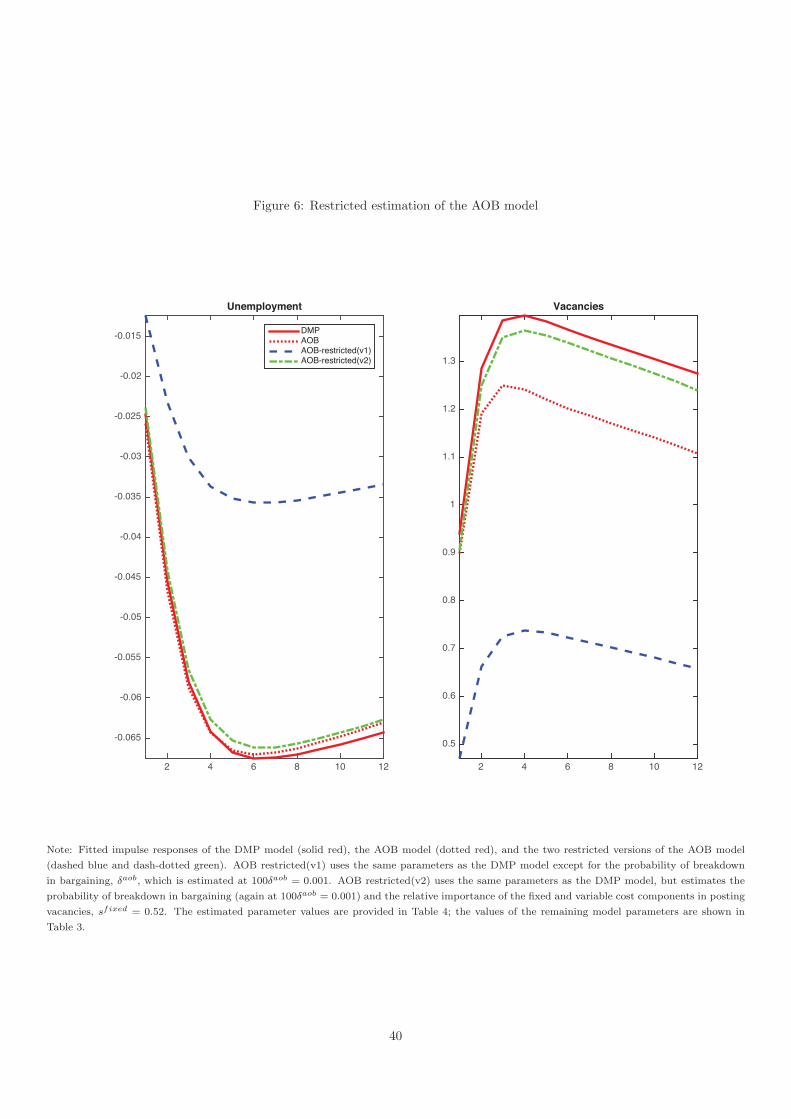
Figure 6: Restricted estimation of the AOB model
2 4 6 8 10 12
-0.065
-0.06
-0.055
-0.05
-0.045
-0.04
-0.035
-0.03
-0.025
-0.02
-0.015
Unemployment
DMPAOBAOB-restricted(v1)AOB-restricted(v2)
2 4 6 8 10 12
0.5
0.6
0.7
0.8
0.9
1
1.1
1.2
1.3
Vacancies
Note: Fitted impulse responses of the DMP model (solid red), the AOB model (dotted red), and the two restricted versions of the AOB model
(dashed blue and dash-dotted green). AOB restricted(v1) uses the same parameters as the DMP model except for the probability of breakdown
in bargaining, δaob, which is estimated at 100δaob = 0.001. AOB restricted(v2) uses the same parameters as the DMP model, but estimates the
probability of breakdown in bargaining (again at 100δaob = 0.001) and the relative importance of the fixed and variable cost components in posting
vacancies, sfixed = 0.52. The estimated parameter values are provided in Table 4; the values of the remaining model parameters are shown in
Table 3.
40

Figure
7:Sen
sitivityto
financialmarket
arrangem
ents,tradeopen
ness,
andsubstitutabilityofgoods
24
68
1012
0.050.
1
0.150.
2
Do
mes
tic
Ab
sorp
tio
n
DM
P b
asel
ine
Fin
. aut
arch
yO
pen
Eco
nom
y P
IH m
odel
24
68
1012
-0.1
8
-0.1
6
-0.1
4
-0.1
2
-0.1
-0.0
8
-0.0
6
-0.0
4
-0.0
2
Un
emp
loym
ent
24
68
1012
0.51
1.52
2.53
3.54
4.5
Vac
anci
es
24
68
1012
0
0.2
0.4
0.6
0.81
Tra
de
bal
ance
24
68
1012
-1.6
-1.4
-1.2-1
-0.8
-0.6
-0.4
-0.20
Exc
han
ge
rate
24
68
1012
0.10
5
0.11
0.11
5
0.12
0.12
5
0.13
0.13
5
Do
mes
tic
Ab
sorp
tio
n
DM
P b
asel
ine
Low
trad
e el
astic
ityH
igh
trad
e sh
are
24
68
1012
-0.0
9
-0.0
8
-0.0
7
-0.0
6
-0.0
5
-0.0
4
-0.0
3
Un
emp
loym
ent
24
68
1012
1
1.2
1.4
1.6
1.8
Vac
anci
es
24
68
1012
0
0.2
0.4
0.6
0.8
Tra
de
bal
ance
24
68
1012
-0.6
-0.5
-0.4
-0.3
-0.2
-0.1
Exc
han
ge
rate
Note:Thetop
panel
illustratesth
esensitivityofth
eestimated
DMP
model
toch
anges
inth
edeg
reeofintern
ationalrisk
sharing.Financialautarky(d
ash
-dotted
green
)refers
toa
calibrationofth
ebaselinemodel
whereth
ebondholdingco
stparameter,φb,is
approach
inginfinity.
Theopen
economyPIH
model
(dash
edblue)
correspondsto
aca
librationofth
e
baselinemodel
whereφb≈
0.Thebottom
panel
illustratessensitivitywhen
theeconomyis
more
open
(dash
edblue)
bysetting
exh ss
gdpss=
0.15andwhen
thehomeandforeigngoodare
less
substitutable
(dash
-dotted
green
),θ=
0.8.In
theestimatedDMP
model
(red
inallpanels)
theco
rrespondingvalues
are
φb=
0.845,
exh ss
gdpss=
0.05,andθ=
2.Domesticabsorp
tion
isco
mputedasth
eweightedaverageofco
nsu
mptionandinvestm
ent.
41
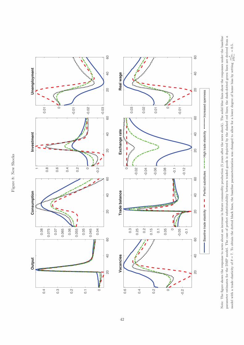
Figure
8:New
Shocks
2040
60
0
0.1
0.2
0.3
0.4
Ou
tpu
t
Bas
elin
e tr
ade
elas
ticity
Per
fect
sub
stitu
tes
Hig
h tr
ade
elas
ticity
Incr
ease
d op
enne
ss
2040
60
0.04
0.04
5
0.05
0.05
5
0.06
0.06
5
0.07
0.07
5
0.08
Co
nsu
mp
tio
n
2040
60
-0.20
0.2
0.4
0.6
0.81
Inve
stm
ent
2040
60-0
.03
-0.0
2
-0.0
10
0.01
Un
emp
loym
ent
2040
60
-0.20
0.2
0.4
0.6
Vac
anci
es
2040
60
-0.1
-0.0
50
0.050.
1
0.150.
2
0.250.
3
Tra
de
bal
ance
2040
60
-0.1
2
-0.1
-0.0
8
-0.0
6
-0.0
4
-0.0
20
Exc
han
ge
rate
2040
60
-0.0
10
0.01
0.02
0.03
Rea
l wag
e
Note:Thefigure
showsth
eresp
onse
tonew
saboutanincrea
sein
futu
reco
mmodityproduction(5
yea
rsafter
thenew
ssh
ock
).Thesolidbluelines
show
theresp
onsesunder
thebaseline
parameter
estimatesforth
eDMP
model.Theca
seofperfect
substitutabilitybetweentraded
goodsis
dep
ictedbyth
edash
edredlines;th
edash
-dotted
green
lines
are
derived
from
a
model
withatradeelasticityofθ=
7.Toobtain
thedotted
black
lines,th
ebaselineparameterizationwasch
anged
toallow
foralower
deg
reeofhomebiasbysetting
exh ss
gdpss=
0.5.
42

Figure 9: labour market tightness — data and model predictions
0 2 4 6 8 10 12-0.5
0
0.5
1
1.5
2
2.5
datamodel approximation
Note: The blue line depicts the response of labour market tightness constructed directly from the VAR estimates. The dashed red line is the
predicted response of labour market tightness using equation (65) based on the empirical responses of the real exchange rate and labour market
productivity.
43

Table 1: Share of top three commodity exports
% of country % of worldnet exports net exports
Australia
Iron ores and concentrates 33 50Coal; briquettes 18 35Petroleum gases 8 6
Canada
Petroleum oils, crude 30 5Petroleum gases 4 3Wheat and meslin 4 16
New Zealand
Milk & cream concentrated 24 37Lamb meat 8 43Butter 7 44
Norway
Petroleum oils, crude 43 3Petroleum gases 24 8Fish, excluding fillets 7 62
Notes: Source: Harvard Atlas of Economic Complexity, 2014 data.
Table 2: Volatilities with respect to output
Variable Australia Canada Norway NZ
Unconditional moments in data[Conditional moments in VAR]
Price of 20.9 10.9 15.6 5.1Commodities [65.9] [65.7] [67.7] [73.1]
Consumption 1.67 0.68 1.22 1.25[1.12] [1.14] [1.31] [1.27]
Investment 7.05 3.82 6.01 5.00[8.29] [8.11] [7.74] [8.97]
Unemployment 0.51 0.41 0.41 0.56rate [0.64] [0.62] [0.61] [0.68]
Vacancies 14.1 10.9 16.9 11.6posted [18.1] [18.6] [17.5] [20.9]
Net trade 1.49 0.87 2.10 0.93[5.69] [5.68] [5.26] [6.21]
Real Exchange Rate 8.97 3.94 2.07 5.61[5.65] [5.93] [6.97] [6.33]
Real wage 2.01 0.91 0.72 0.93[0.67] [0.89] [0.98] [0.97]
Total hours 1.89 0.57 1.06 1.23worked [1.90] [1.88] [1.80] [2.13]
Notes: Unconditional and [conditional on commodity price shocks] standard deviations relative to GDP.
44

Table 3: Calibrated parameters
ModelsParameter Description DMP DMP(l) AOB RBC RBC(rr)
β Discount factor 0.99(all models)
σ Curvature of 1.10utility function (all models)
α Share of capital 0.33(all models)
δ Depreciation rate 0.025(all models)
θ Trade elasticity 2.00(all models)
exhss
gdpssSteady state goods export 0.05
GDP ratio (all models)
ycss
gdpssSteady state commodity export 0.15
GDP ratio (all models)
v Home-bias parameter 0.80(all models) [implied]
nss Steady state 0.95 0.95 0.95 – –employment
qss Steady state prob. 0.7 0.7 0.7 – –of filling vacancy
κvvss+qκyhss
Share of vacancy 0.005 0.005 0.005 – –
cost in output
ρ Probability that 0.1 0.1 0.1 – –match breaks up
bu/wss Replacement ratio 0.4 0.4 0.4 – –
χ Scale parameter 0.67 0.67 0.67 – –in matching function [implied] [implied] [implied]
Notes: DMP = baseline model, DMP(l) = baseline model with elastic labour supply, AOB = alternating offer bargaining model, RBC = Real
business cycle model with Walrasian labour markets, RBC(rr) = RBC model with real wage rigidities.
45

Table 4: Estimated parameters
ModelsParameter Description DMP DMP(l) AOB RBC RBC(rr)
φb Bond holding cost 0.85 0.72 0.86 0.70 0.68(× 100) [0.004] [0.004] [0.004] [0.004] [0.004]
φv Cost of vacancies 1.10 0.96 0.84 – –[0.020] [0.018] [0.027] – –
φ Investment 0.04 0.005 0.04 0.02 0.02adjustment costs [0.001] [0.001] [0.001] [0.001] [0.001]
ζ Matching function 0.72 0.74 0.70 – –parameter [0.001] [0.001] [0.001] – –
δaob AOB parameter – – 0.001 – –(× 100) – – [0.03] – –
cuss/cwss Consumption share 0.60 0.58 – – –
of the unemployed [0.000] [0.000] – – –
sfixed Fixed cost of bargaining 0.001 0.001 0.46 – –[0.03] [0.03] [0.03] – –
ξ Household’s 0.40 0.30 – – –bargaining weight [implied] [implied]
φ Inverse of labour – 0.74 – 0.48 0.93supply elasticity – [implied] – [0.003] [0.01]
η Real wage rigidity – – – – 0.84– – – – [0.003]
Notes: DMP = baseline model, DMP(l) = baseline model with elastic labour supply, AOB = alternating offer bargaining model, RBC = Real
business cycle model with Walrasian labour markets, RBC(rr) = RBC model with real wage rigidities. Numbers in brackets are standard errors.
46

A Additional details for econometric analysis
A.1 Data description and definitions
Table 5 lists the raw data used in the VARs. All series are taken from Haver Analytics, and the data set is
available upon request from the authors. For each country in the panel, ten time series are used, which are
transformations of the raw data:
pcor = ln
(COM
US CPI
)(A.1)
y = ln
(GDP
POP
)(A.2)
c = ln
(C
POP
)(A.3)
i = ln
(I
POP
)(A.4)
nxm =
(NXE
GDP (L)
)(A.5)
urate =
(UNE
LAF
)(A.6)
vac = ln(V AC) (A.7)
fxr = ln(REER) (A.8)
wprr = ln
(WAGE
CPI
)(A.9)
thp = ln
(Total HRS
POP
). (A.10)
47

Tab
le5:
Data
defi
nitions
Data
sources
Raw
Data
Australia
Canada
New
Zealand
Norw
ay
GDP
GDP
(SA,Mil.C
hn.A
$)
GDP
(SA,Mil.C
hn.C$)
GDP
(SA,Mil.C
hn.N
Z$)
GDP
(SA,Mil.C
hn.N
OK)
GDP(L
)GDP
(SA,Mil.A
$)
GDP
(SA,Mil.C
$)
GDP
(SA,Mil.N
Z$)
GDP(SA,Mil.K
roner)
CHHsCons.
Exp.(SA,Mil.C
hn.A
$)
PersonalCons.
Exp.(SA,Mil.C
hn.C
$)
Priv.Cons.
Exp.(SA,Mil.C
hn.N
Z$)
Priv.Cons.
Exp.(SA,Mil.C
hn.N
OK)
IPrivFixed
Cap.Form
.(SA,Mil.C
hn.A
$)
Bus.
Fixed
Inv.(SA,Mil.C
hn.C
$)
Gross
Fixed
Cap.Form
.(SA,Mil.C
hn.N
Z$)
Priv.Fixed
Cap.Form
.(SA,Mil.C
hn.N
OK)
NEX
Net
Exportsof
GoodsandServ.(SA,Mil.A
$)
Net
ExportsofGoodsandServ.(SA,Mil.C
$)
Net
ExportsofGoodsandServ.(SA,Mil.N
Z$)
Net
Exports
ofGoodsandServ.(SA,Mil.K
roner)
UNE
Unem
p.:AllPers.
15an
dOver(SA,1000s)
AllPers.
15an
dOver
(SA,1000s)
AllPers.
15an
dOver
(SA,1000s)
RegisteredUnem
p.(SA,EOP,Number)
LAF
LaborForce:
AllPers15andOver
(SA,1000s)
LaborForce:
AllPers15andOver(SA,1000s)
LaborForce:
AllPers15andOver(SA,1000s)
LaborForce(SA,1000s)
VAC
Unfilled
JobVacancies
(SA,Number)
Vacancies
(A.Tasci)(SA)
ANZJobAds(SA)
Unfilled
JobVacancies
(SA,Number)
REER
RealEffective
ExchangeRate
RealEffective
ExchangeRate
RealEffective
ExchangeRate
RealEffectiveExchangeRate
WAGE
EarlyEst
LaborComp
SameasAustralia
SameasAustralia
SameasAustralia
Per
UnitLaborInput:
TotEcon(SA)
TotalHRS
Totalhours
(SA)
Totalhours(SA)
Totalhours
(SA)
Totalhours
(SA)
COM
RBA
CommodityPrices:
AllItem
s:US$(N
SA)
BoC
CommodityPrice
Index
ANZWorld
CommodityPrice
Index
(US$,NSA)
BrentCrudeOil(U
S$/Barrel)
POP
PopulationPersons(SA)
Pop
ulationPersons(SA)
Pop
ulationPersons(SA)
PopulationPersons(SA)
CPI
CPI:allitem
sexlc
Food&
Energy(N
SA)
Consumer
Price
Index
(NSA)
Consumer
Price
Index
(NSA)
EuropeanHarm
onized
CPI(N
SA)
USCPI
USCPI(SA)
USCPI(SA)
USCPI(SA)
USCPI(SA)
Notes:
Source:
Alldata
are
taken
from
Haver
Analytics.
48
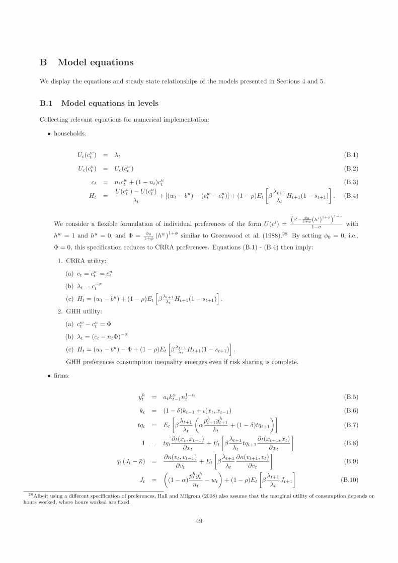
B Model equations
We display the equations and steady state relationships of the models presented in Sections 4 and 5.
B.1 Model equations in levels
Collecting relevant equations for numerical implementation:
• households:
Uc(cwt ) = λt (B.1)
Uc(cut ) = Uc(c
wt ) (B.2)
ct = ntcwt + (1− nt)c
ut (B.3)
Ht =U(cwt )− U(cut )
λt+ [(wt − bu)− (cwt − cut )] + (1− ρ)Et
[βλt+1
λtHt+1(1− st+1)
]. (B.4)
We consider a flexible formulation of individual preferences of the form U(ci) =
(ci− φ0
1+φ (hi)
1+φ)1−σ
1−σ with
hw = 1 and hu = 0, and Φ = φ0
1+φ (hw)1+φ
similar to Greenwood et al. (1988).28 By setting φ0 = 0, i.e.,
Φ = 0, this specification reduces to CRRA preferences. Equations (B.1) - (B.4) then imply:
1. CRRA utility:
(a) ct = cwt = cut
(b) λt = c−σt
(c) Ht = (wt − bu) + (1− ρ)Et
[β λt+1
λtHt+1(1− st+1)
].
2. GHH utility:
(a) cwt − cut = Φ
(b) λt = (ct − ntΦ)−σ
(c) Ht = (wt − bu)− Φ+ (1− ρ)Et
[β λt+1
λtHt+1(1− st+1)
].
GHH preferences consumption inequality emerges even if risk sharing is complete.
• firms:
yht = atkαt−1n
1−αt (B.5)
kt = (1− δ)kt−1 + ι(xt, xt−1) (B.6)
tqt = Et
[βλt+1
λt
(αpht+1y
ht+1
kt+ (1− δ)tqt+1
)](B.7)
1 = tqt∂ι(xt, xt−1)
∂xt+ Et
[βλt+1
λttqt+1
∂ι(xt+1, xt)
∂xt
](B.8)
qt (Jt − κ) =∂κ(vt, vt−1)
∂vt+ Et
[βλt+1
λt
∂κ(vt+1, vt)
∂vt
](B.9)
Jt =
((1− α)
pht yht
nt− wt
)+ (1− ρ)Et
[βλt+1
λtJt+1
](B.10)
28Albeit using a different specification of preferences, Hall and Milgrom (2008) also assume that the marginal utility of consumption depends onhours worked, where hours worked are fixed.
49

ι(xt, xt − 1) = κxxt
(1− φx
2
(xt
xt−1− 1
)2)
(B.11)
∂ι(xt, xt−1)
∂xt=
ι(xt, xt−1)
xt− κxφx
(xt
xt−1− 1
)xt
xt−1(B.12)
∂ι(xt, xt−1)
∂xt−1= κxφx
(xt
xt−1− 1
)(xt
xt−1
)2
(B.13)
κ(vt, vt−1) = κvvt
(1 +
φv
2
(vt
vt−1− 1
)2)
(B.14)
∂κ(vt, vt−1)
∂vt=
κ(vt, vt−1)
vt+ κvφv
(vt
vt−1− 1
)vt
vt−1(B.15)
∂κ(vt, vt−1)
∂vt−1= −κvφv
(vt
vt−1− 1
)(vt
vt−1
)2
(B.16)
If κ = 0 and φv = 0, the equations reduce to their standard formulations.
• trade in goods and assets:
1
1 + rt= Et
[βλt+1
λt
rert+1
rert
](B.17)
v(pht
)1−θ= 1− (1− v) (rert)
1−θ(B.18)
yht = v(pht
)−θ(ct + xt + κqt + κ (vt, vt−1)) + exh
t (B.19)
exht = v∗
(rertpht
)θ∗
y∗t (B.20)
tbalt = 1− ct + xt + κqt + κ(vt, vt−1)
gdpt(B.21)
bt = (1 + rt−1)gdpt−1
gdpt
rertrert−1
bt−1 + tbalt (B.22)
1 + rt = (1 + r∗t ) e−φb(bt−b) (B.23)
gdpt = rertpc∗t yct + pht y
ht . (B.24)
where tbalt is the trade balance to GDP ratio. Net foreign assets relative to GDP, bt, are given by bt =rertbtgdpt
.
• search and matching:
mt = χuζt v
1−ζt (B.25)
nt = (1− ρ)nt−1 +mt (B.26)
ut = 1− (1− ρ)nt−1 (B.27)
ut = 1− nt (B.28)
θt =vtut
(B.29)
st = χθ1−ζt (B.30)
qt = χθ−ζt (B.31)
• exogenous variables: at, pc∗t , yct , r
∗t , y
∗t .
50
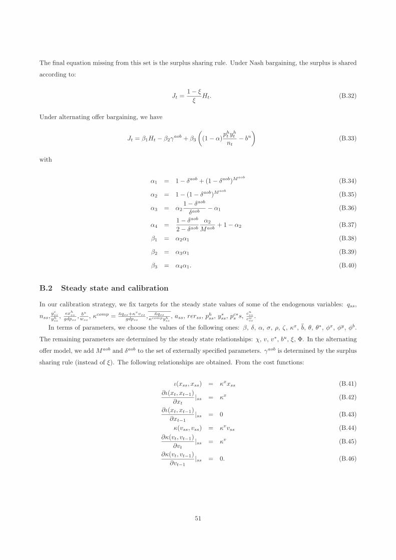
The final equation missing from this set is the surplus sharing rule. Under Nash bargaining, the surplus is shared
according to:
Jt =1− ξ
ξHt. (B.32)
Under alternating offer bargaining, we have
Jt = β1Ht − β2γaob + β3
((1− α)
pht yht
nt− bu
)(B.33)
with
α1 = 1− δaob + (1− δaob)Maob
(B.34)
α2 = 1− (1− δaob)Maob
(B.35)
α3 = α21− δaob
δaob− α1 (B.36)
α4 =1− δaob
2− δaobα2
Maob+ 1− α2 (B.37)
β1 = α2α1 (B.38)
β2 = α3α1 (B.39)
β3 = α4α1. (B.40)
B.2 Steady state and calibration
In our calibration strategy, we fix targets for the steady state values of some of the endogenous variables: qss,
nss,ycss
yhss,
exhss
gdpss, bu
wss, κcomp = κqss+κvvss
gdpss, κqssκcompyh
ss, ass, rerss, p
hss, y
∗ss, p
c∗s s,
cusscwss
.
In terms of parameters, we choose the values of the following ones: β, δ, α, σ, ρ, ζ, κx, b, θ, θ∗, φx, φy, φb.
The remaining parameters are determined by the steady state relationships: χ, v, v∗, bu, ξ, Φ. In the alternating
offer model, we add Maob and δaob to the set of externally specified parameters. γaob is determined by the surplus
sharing rule (instead of ξ). The following relationships are obtained. From the cost functions:
ι(xss, xss) = κxxss (B.41)
∂ι(xt, xt−1)
∂xt|ss = κx (B.42)
∂ι(xt, xt−1)
∂xt−1|ss = 0 (B.43)
κ(vss, vss) = κvvss (B.44)
∂κ(vt, vt−1)
∂vt|ss = κv (B.45)
∂κ(vt, vt−1)
∂vt−1|ss = 0. (B.46)
51
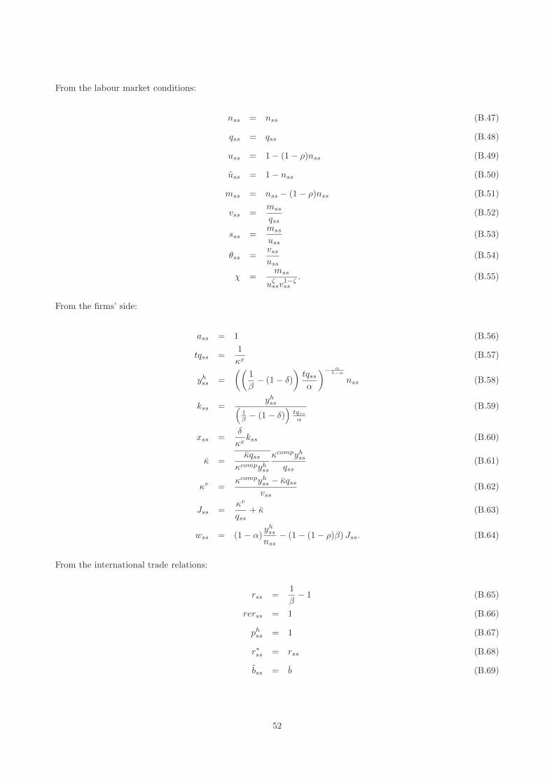
From the labour market conditions:
nss = nss (B.47)
qss = qss (B.48)
uss = 1− (1− ρ)nss (B.49)
uss = 1− nss (B.50)
mss = nss − (1− ρ)nss (B.51)
vss =mss
qss(B.52)
sss =mss
uss(B.53)
θss =vssuss
(B.54)
χ =mss
uζssv
1−ζss
. (B.55)
From the firms’ side:
ass = 1 (B.56)
tqss =1
κx(B.57)
yhss =
((1
β− (1− δ)
)tqssα
)− α1−α
nss (B.58)
kss =yhss(
1β − (1− δ)
)tqssα
(B.59)
xss =δ
κxkss (B.60)
κ =κqss
κcompyhss
κcompyhssqss
(B.61)
κv =κcompyhss − κqss
vss(B.62)
Jss =κv
qss+ κ (B.63)
wss = (1− α)yhssnss
− (1− (1− ρ)β) Jss. (B.64)
From the international trade relations:
rss =1
β− 1 (B.65)
rerss = 1 (B.66)
phss = 1 (B.67)
r∗ss = rss (B.68)
bss = b (B.69)
52

tbalss = bss − (1 + rss) bss (B.70)
pc∗ss = 1 (B.71)
gdpss =
(ycssyhss
+ 1
)yhss (B.72)
v∗ =exh
ss
y∗ss. (B.73)
From the household side:
css = (1− tbalss) gdpss − (xss + κqss + κvvss) (B.74)
v =yhss − exh
ss
css + xss + κqss + κvvss(B.75)
λss = c−σss
(nss
(cwsscuss
)+ (1− nss)
)σ
(B.76)
Hss =−Φ+ wss − bu
1− (1− ρ)β(1− sss). (B.77)
The bargaining sharing rule determines the bargaining weight:
ξ =Hss
Jss +Hss. (B.78)
An alternative approach is to fix the bargaining weight and then compute the replacement ratio. We use the
bargaining sharing rule to solve for Hss and then use the equation defining Hss to solve for bu.
Finally, the calibration of Φ is linked to the choice ofcwsscuss
:
Φ =
cwsscuss
− 1
nss
(cwsscuss
)+ (1− nss)
css. (B.79)
Under alternating offer bargaining the additional restriction needed determines γaob:
γaob =1
β2
(β1Hss − Jss + β3
((1− α)
yhssnss
− bu))
. (B.80)
B.3 Search and matching model with elastic labour supply
The overwhelming share of the labour search literature assumes that labour is supplied inelastically. By contrast
models without search and matching frictions always model the labour supply as elastic. Here we consider the
case of an elastic labour supply in the search and matching framework under the assumption of complete risk
sharing among household members. If the labour supply is elastic, the marginal value of employment to the
household is given by:
Ht =U(cwt )− U(cut )
λt+ wth
wt − bu − (cwt − cut ) + (1− ρ)Et
[βλt+1
λtHt+1(1− st+1)
]. (B.81)
53

We replace the marginal value of employment to the firms by:
Jt =
((1− α)
pht yht
nthwt
hwt − wth
wt
)+ (1− ρ)Et
[βλt+1
λtJt+1
](B.82)
and the production function by:
yht = atkαt−1(nth
wt )
1−α. (B.83)
Nash bargaining occurs over wages and hours worked, yielding the conditions:
Jt =1− ξ
ξHt (B.84)
−Uwh (cwt , h
wt )
λt= (1− α)
pht yht
nthwt
. (B.85)
In deriving equation (B.85), we assume that the household member and the firm take λt and the marginal product
of the firm mplt = (1−α)pht y
ht
nthwtas given in negotiating over hours worked as in Cheron and Langot (2004). Under
this assumption the marginal rate of substitution between labour and consumption equals the marginal product
of labour.
With GHH preferences and no labour effort by unemployed households, full risk sharing implies:
cwt − cut =φ0
1 + φ(hw
t )1+φ
U(cwt )− U(cut )
λt=
1
1− σ
(cwt − cut − φ0
1 + φ(hw
t )1+φ
)= 0.
Consequently, the following conditions prevail:
cwtcut
= 1 +
(nt
(cwtcut
)+ (1− nt)
) φ0
1+φ (hwt )
1+φ
ct(B.86)
λt = c−σt
(nt
(cwtcut
)+ (1− nt)
)σ
(B.87)
Ht = wthwt − bu − φ0
1 + φ(hw
t )1+φ
+ (1− ρ)Et
[βλt+1
λtHt+1(1− st+1)
]φ0 (h
wt )
φ= (1− α)
pht yht
nthwt
(B.88)
54
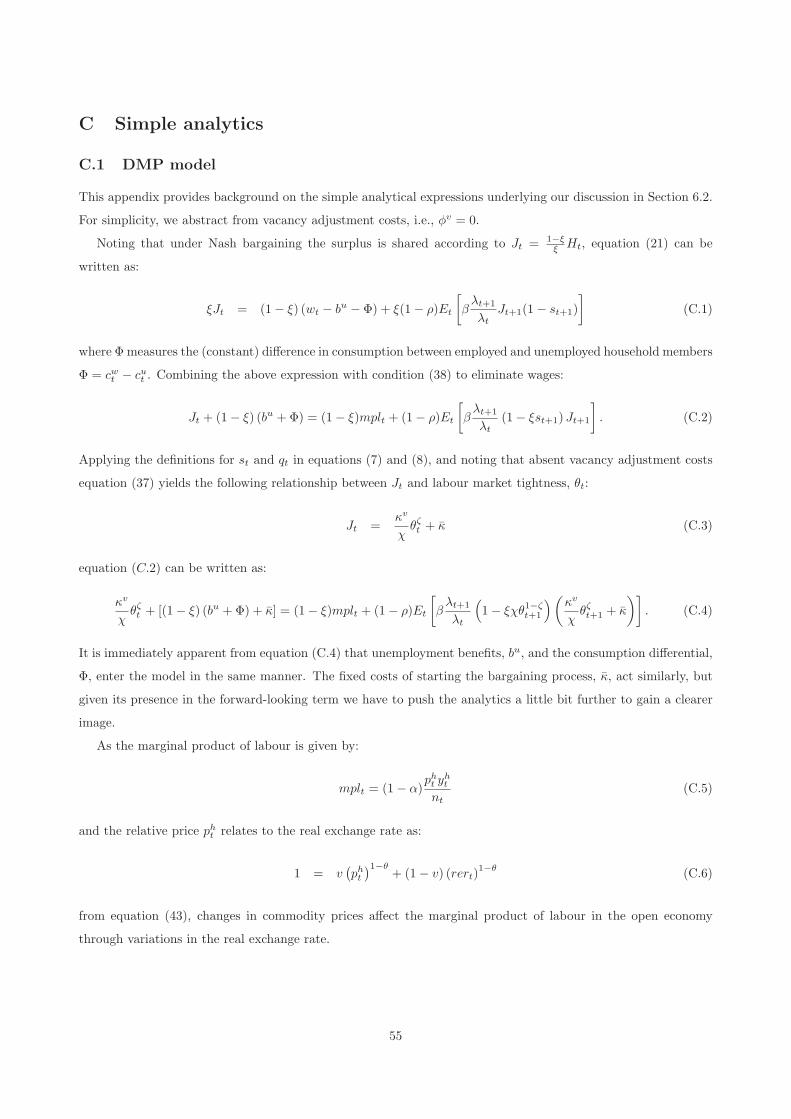
C Simple analytics
C.1 DMP model
This appendix provides background on the simple analytical expressions underlying our discussion in Section 6.2.
For simplicity, we abstract from vacancy adjustment costs, i.e., φv = 0.
Noting that under Nash bargaining the surplus is shared according to Jt = 1−ξξ Ht, equation (21) can be
written as:
ξJt = (1− ξ) (wt − bu − Φ) + ξ(1− ρ)Et
[βλt+1
λtJt+1(1− st+1)
](C.1)
where Φ measures the (constant) difference in consumption between employed and unemployed household members
Φ = cwt − cut . Combining the above expression with condition (38) to eliminate wages:
Jt + (1− ξ) (bu +Φ) = (1− ξ)mplt + (1− ρ)Et
[βλt+1
λt(1− ξst+1) Jt+1
]. (C.2)
Applying the definitions for st and qt in equations (7) and (8), and noting that absent vacancy adjustment costs
equation (37) yields the following relationship between Jt and labour market tightness, θt:
Jt =κv
χθζt + κ (C.3)
equation (C.2) can be written as:
κv
χθζt + [(1− ξ) (bu +Φ) + κ] = (1− ξ)mplt + (1− ρ)Et
[βλt+1
λt
(1− ξχθ1−ζ
t+1
)(κv
χθζt+1 + κ
)]. (C.4)
It is immediately apparent from equation (C.4) that unemployment benefits, bu, and the consumption differential,
Φ, enter the model in the same manner. The fixed costs of starting the bargaining process, κ, act similarly, but
given its presence in the forward-looking term we have to push the analytics a little bit further to gain a clearer
image.
As the marginal product of labour is given by:
mplt = (1− α)pht y
ht
nt(C.5)
and the relative price pht relates to the real exchange rate as:
1 = v(pht
)1−θ+ (1− v) (rert)
1−θ(C.6)
from equation (43), changes in commodity prices affect the marginal product of labour in the open economy
through variations in the real exchange rate.
55

Log-linearising expression (C.4) around the steady state, delivers
ζκv
χθζssθt − (1− ρ)β
(ζκv
χθζss − ξκvθss − κξχ(1− ζ)θ1−ζ
ss
)Etθt+1
= (1− ξ)mplssmplt + (1− ρ)β(1− ξχθ1−ζ
ss
)(κv
χθζss + κ
)Et
[λt+1 − λt
]. (C.7)
Given our strategy of keeping the steady state value of the job filling probability identical across calibrations, we
make use of the fact qss = χθ−ζss , and we apply the definition of the marginal product of labour in our simplified
environment to arrive at:
ζκv
qss
(θt − Etθt+1
)+
[(κv
qss+ κ
)[ζ − (1− ρ)β (ζ − qssξθss)]− ζκ [1− (1− ρ)β (1− qssξθss)]
]Etθt+1
= (1− ξ)mplss
(yht − nt − 1− ν
νrert
)+ (1− ρ)β
(κv
qss+ κ
)(1− ξqssθss)Et
[λt+1 − λt
]. (C.8)
In the steady state, equation (C.4) implies:
(κv
qss+ κ
)[1− (1− ρ)β (1− qssξθss)] = (1− ξ) [mplss − (bu +Φ)] . (C.9)
Our strategy of parameterising the DMP model implies assigning a value to the replacement ratio, ru, rather
than unemployment benefits, bu. The definition of the replacement ratio and condition (38) yield the following
unemployment benefits given the replacement ratio:
bu = ruwss = ru(mplss − (1− (1− ρ)β)
(κv
qss+ κ
)). (C.10)
After substituting (C.10) into equation (C.11), we obtain the household bargaining weight, ξ, as an implicit
function of the replacement ratio, ru, and the consumption difference between employed and unemployed, Φ:
(κv
qss+ κ
)[1− (1− ρ)β (1− qssξθss)] = (1− ξ)
[(1− ru)mplss + ru (1− (1− ρ)β)
(κv
qss+ κ
)− Φ
](C.11)
or solved for ξ:
ξ =1
1 +(1−(1−ρ)β(1−qssθss))( κv
qss+κ)
(1−ru)(mplss−(1−(1−ρ)β)( κv
qss+κ))−Φ
. (C.12)
ξ is decreasing in ru and Φ.29
For convenience, we define the coefficient Υ as:
Υ =
(κv
qss+ κ
)[ζ − (1− ρ)β (ζ − qssξθss)]− ζκ [1− (1− ρ)β (1− qssξθss)](
κv
qss+ κ
)[1− (1− ρ)β (1− qssξθss)]
= ζ + (1− ζ)(1− ρ)βqssξθss
1− (1− ρ)β (1− qssξθss)− ζ
κκv
qss+ κ
. (C.13)
29It is worth pointing out that for common calibration choice of the other parameters it is much easier to obtain an implied bargaining weightaround 0.5 at a moderate replacement ratio if Φ > 0.
56

Only the second term in Υ depends on ξ; therefore Υ is bounded by ζ − ζ κκv
qss+κ
(for ξ = 0) and 1− ζ κκv
qss+κ
.
With these expressions in hand, we can approximate the response of labour market tightness to a commodity
price shock. To avoid complications from transition dynamics, we focus on the “medium run”. The commodity
price shock induces highly persistent movements in the endogenous variables, thus implying little change in the
endogenous variables from one period to another after the initial transition. Applying this reasoning to equation
(C.7), the following approximate relationship between labour market tightness, labour productivity, and the real
exchange rate emerges:
θt = vt − ut ≈ 1
Υ
mplss
(1− ru)mplss + ru (1− (1− ρ)β)(
κv
qss+ κ
)− Φ
(yht − nt − 1− ν
νrert
). (C.14)
The impact of given changes in the real exchange rate onto labour market tightness is determined by the interplay
of the parameters ru and Φ.30 For now, we abstract from the coefficients κ and κv. Although Υ is a function
of ξ and therefore depends on the choices of ru and Φ as is apparent from equation (C.12), the role of this
coefficient in delivering big amplification of the exchange rate movement is limited since Υ is bounded. For κ = 0,
Υ ∈ [ζ, 1]. Much more powerful in delivering amplification are therefore the parameters ru and Φ. An increase in
the replacement ratio or in the consumption gap between employed and unemployed household members reduces
the denominator of the second coefficient and results in bigger movements of labour market tightness for a given
movement of the real exchange rate. It is for this interplay of the parameters ru and Φ that our model can match
the responses in unemployment and vacancies even for a moderate value of the replacement ratio of ru = 0.4.
The choice of the parameter κ also influences the transmission of the shock to labour market tightness. Our
calibration strategy imposes a tight relationship with κv as we target a specific value of the total (expected) costs
of vacancy posting, κvvss+qssκ, relative to non-commodity output in the steady state, yhss. Thus, the termκ
κv
qss+κ
equals sfixed
1−sfixed
vss+sfixed
, where sfixed is the share of vacancy posting costs that falls onto qssκ. By increasing sfixed,
the term κκv
qss+κ
in (C.13) increases and implies a lower value of Υ. However, it can also be shown that raising
sfixed implies a lower value of κv
qss+ κ and a higher value of the Nash bargaining weight ξ. This effect in turn,
raises the value of the second term in equation (C.13) and raises the value of Υ. Numerically, raising sfixed fails
to deliver sufficient amplification.
The most effective way of raising the impact of given a change in the real exchange rate on labour market
tightness is therefore to allow for preferences that are non-separable in consumption and leisure to justify a
consumption gap between the employed and unemployed household members, i.e., Φ > 0. This approach avoids
having to set the replacement ratio to unrealistically high levels and is by far more effective than raising the share
of the fixed costs of bargaining in the overall vacancy posting costs, sfixed.
30Recall, that ut measure the pool of job-seekers at the beginning of the period and not the unemployment rate which is measured by ut. In the
medium run, the two concepts are related via ut ≈ 1−(1−ρ)nss−ρ1−(1−ρ)nss
ˆut.
57

C.2 AOB model
As in the DMP model, we can derive an equation describing the evolution of labour market tightness for the AOB
model. The bargaining sharing rule implies:
Jt =β1 + β3
1 + β1
(mplt − bu − β2
β1 + β3γaob
)+ (1− ρ)Et
[βλt+1
λt
(1− 1
1 + β1st+1
)Jt+1
]−(1− ρ)Et
[βλt+1
λt(1− st+1)
β3
1 + β1
(mplt+1 − bu − β2
β3γaob
)]. (C.15)
We proceed as under the DMP model to obtain a better understanding how labour market tightness is affected
by commodity price shocks. In the steady state, equation (C.15) implies:
(κv
qss+ κ
)[1− (1− ρ)β
(1− 1
1 + β1qssθss
)]− β1
1 + β1
β2
β3γaob
=
(β1
1 + β1+
β3
1 + β1[1− (1− ρ)β (1− qssθss)]
)(mplss − bu − β2
β3γaob
). (C.16)
Given the values of δaob and Maob, the parameters β1, β2, β3 are determined as demonstrated in Section 5.2.
Furthermore, our calibration strategy of targeting qss and nss (and therefore θss) implies that γaob is a function
of κv and κ. The parameter γaob is not a free parameter.
We approximate the impact of a given change in the real exchange rate on labour market tightness over the
medium term as:
θt =
β1
1+β1
β2
β3γaob − Ω2
Ω1 − (1− ρ)βqssθss(1− ζ) β3
1+β1
(mplss − bu − β2
β3γaob
) mplss
mplss − bu − β2
β3γaob
(yht − nt − 1− ν
νrer
)(C.17)
where
Ω1 =
(κv
qss+ κ
)[ζ − (1− ρ)β
(ζ − 1
1 + β1qssθss
)]− ζκ
[1− (1− ρ)β
(1− 1
1 + β1qssθss
)](C.18)
Ω2 =
(κv
qss+ κ
)[1− (1− ρ)β
(1− 1
1 + β1qssθss
)]. (C.19)
As under the DMP model, the impact of a given change in the real exchange rate on labour market tightness is
bigger for higher values of the replacement ratio:
bu = ruwss = ru(mplss − (1− (1− ρ)β)
(κv
qss+ κ
)). (C.20)
The important question is, however, to what extent can the model amplify the response of labour market tightness
for a moderate value of the replacement ratio? The free parameters in the alternating offer bargaining model are:
δaob, Maob, and sfixed.31
To maximize the impact of the shock, it is advisable to:
• maximize the term β2
β3γaob to raise mplss
mplss−bu− β2β3
γaob
31Recall that sfixed measures the share of the overall vacancy posting costs apportioned to qssκ in our calibration.
58

• minimize β1 to increase the term Ω2 − β1
1+β1
β2
β3γaob,
• and maximize β3 to reduce the term Ω1 − (1− ρ)βqssθss(1− ζ) β3
1+β1
(mplss − bu − β2
β3γaob
).
Setting a low probability of breakdown in bargaining, δaob achieves the second and third point. With regard to
the first point, note from equation (C.16), the term β2
β3γaob increases in the value of sfixed for given Maob and
δaob.
Our estimation results confirm the conjecture that β1 is ideally set close to zero given the calibration of the
total cost of vacancy posting. Across different calibrations, our point estimate for the probability δaob is always
close to zero.32 If δaob ≈ 0, the bargaining equation reduces to:
Jt ≈ −β2γaob + β3(mplt − bu) (C.21)
or in log-linearised form:
θt =β3mplssζ κv
qss
(yht − nt − 1− ν
νrert
). (C.22)
In this case, the wage sharing rule is (close to) independent of the marginal value of employment to the household,
Ht. Equation (C.22) reveals the importance of sfixed in the alternating offer bargaining model. For a higher value
of sfixed, we obtain that the share of total vacancy posting costs accounted for by the variable component κvvss
is smaller. The resulting value of κv will also be smaller. For sfixed sufficiently large, the model can deliver the
desired amplification of the labour market tightness response of a given real exchange rate movement. Note, that
restricting sfixed to zero very much restricts the empirical performance of the model.
It is noteworthy, that had we assumed a much lower value of the total vacancy posting costs relative to output,
κvvss+qssκyhss
, the estimated value δaob would have been further away from zero, but sfixed would have been close
to zero. In the case of low vacancy posting costs, the implied value of κv might be so small — even for sfixed = 0
— that the amplification of labour market tightness is too big relative to the data. In this case, the coefficient
β3mplssζ κv
qss
needs to be lowered by reducing β3, i.e., allowing for a larger value of δaob. Although in this case, Ht
reenters the analysis and the simplified formula in equation (C.22) no longer applies directly, the intuition just
laid out applies.
The sensitivity of the parameter estimates to the calibration of the total vacancy posting costs relative to
output, κvvss+qssκyhss
, is unique to the alternating offer bargaining model. In the DMP model a drastic reduction in
these costs barely influences the parameter estimates; in particular the DMP model always favours sfixed close
to zero.
32Using a different procedure, Christiano et al. (2013) also estimate the probability of breakdown in bargaining to be close to zero.
59