commitment and the time structure of taxation of foreign direct investment

International Tax and Public Finance, 3:479M-94 (1996) �9 1996 Kluwer Academic Publishers

Commitment and the Time Structure of Taxation of Foreign Direct Investment*

MARIANNE VIGNEAULT Bishop's Universit), Lennoxville, Quebec, Canada, JIM IZ7

Abs t rac t

The paper examines the role of commitment to future tax policy as an explanation for tax incentives for foreign direct investment that take the form of rates that increase over time. Both commitment and non-commitment to future tax rates are analyzed using a two-period model with investment determined endogenously in the first period. Without commitment, it is shown that tax rates may increase or decrease with time depending on the relative values of the firms' outside option each period of investing elsewhere in the world and on the responsiveness of investment to a change in the tax rate. With commitment, the time structure of tax rates is shown to depend on the relative rates at which firms and governments discount the future.

JEL Classification: F21, H25, H32

Key words: foreign direct investment, tax incentives, commitment

1. I n t r o d u c t i o n

Fore ign firms are of ten offered tax concess ions of var ious k inds by host count ry g o v e r n m e n t s

w h e n dec id ing whe the r to engage in fore ign di rec t inves tmen t . Tax incen t ives are offered to

encourage f irms to set up opera t ions in the host count ry or to increase the level of i n v e s t m e n t

if p roduc t ion has a l ready begun . One of the mos t c o m m o n incen t ives involves a r educed tax

rate in the ear ly s tages of operat ion. Typically, f irms are g ran ted a tax hol iday where in they

face a zero tax rate for a specif ied per iod of t ime and a posi t ive tax rate af ter this per iod has

expired.

The recent l i terature has offered an a n s w e r to the ques t ion of w h y tax incen t ives for for-

e ign di rec t i n v e s t m e n t f requen t ly take the form of rates tha t increase over t ime as opposed

to, for example , a r educed but cons tan t rate tha t yields the same present va lue tax revenues .

The p remise is that i r revers ib le i n v e s t m e n t c o m b i n e d wi th a host g o v e r n m e n t ' s inabi l i ty to

c o m m i t to future tax rates a l lows the host g o v e r n m e n t to extract a grea te r share of fore ign

*This is a revised version of a chapter of my Ph.D. dissertation completed at Queen's University (1993). I am grateful to my supervisors Robin Boadway and Beverly Lapham for comments on an earlier version. I also thank Sam Bucovetsky and two anonymous referees for comments and suggestions.

480 MARIANNE VIGNEAULT

finn profits through increasing tax rates. This idea has been analyzed theoretically by Doyle and van Wijnbergen (1994). 1 The literature does not, however, address the issue of whether non-commitment is sufficient to yield an increasing tax rate. Nor does the literature examine under what conditions, if any, commitment would give rise to an increasing tax structure. The purpose of this paper is to address these two issues.

Our analysis employs a simple two-period model with the level of capital investment determined endogenously in the first period and remaining fixed thereafter. Both the commitment and non-commitment cases are examined. In contrast to what is suggested in the literature, we find that lack of commitment combined with irreversible investment is neither sufficient nor necessary to yield increasing tax rates. In the non-commitment case, the tax rate may increase or decrease over time if the value of the finns' outside option of investing elsewhere in the second period is not too small relative to that of the first period. If this is the case, an endogenous capital investment decision implies a trade-off for the host government. A higher tax rate, ceteris paribus, generates higher tax revenues. However, a higher tax rate reduces the level of capital which, in turn, reduces the optimal tax rate in the second period. The magnitudes of these last two effects depend on the elasticity of capital with respect to the tax rate in the first period. Our results show that a high elasticity of capital is sufficient to generate an increasing tax structure. This result is intuitive and accords with the optimal tax literature wherein the optimal tax rate varies inversely with elasticity. If, however, capital is not very responsive to a change in the tax rate, we find that a decreasing tax structure is optimal unless the government is constrained in its tax policy by the finns having an outside option of investing elsewhere in the world. This constraint is likely to bind if fixed costs are large and if the value of the outside option of investing elsewhere in the world decreases over time.

The analysis of the commitment case yields the result that the optimal time structure of tax rates depends on the relative rates at which the host government and the finns discount the future. In particular, if the host government discounts the future less than the finns do, the government will levy a reduced tax rate in the first period in anticipation of higher investment and, consequently, higher tax revenues in the second period. While this result may not be particularly surprising, it does offer an alternative explanation for increasing tax rates.

The paper is organized as follows. Section 2 introduces the basic two-period model. Sec- tion 3 examines optimal taxation of foreign direct investment when the host government is able to commit to future tax policy, and Section 4 examines optimal taxation when commitment is not possible. A comparison of the commitment and non-commitment cases is presented in section 5, and section 6 concludes.

2. The model

Consider an economy with a continuum of identical finns which produce a homogeneous good for the world market. Finns have the option of investing in either the host country or another country. We adopt this assumption in order to simplify the model so that the value of the finns' outside option of investing elsewhere is independent of investment in the host

COMMITMENT AND THE TIME STRUCTURE OF TAXATION 481

country. If the firms choose to produce in another country, they earn known profits. If the finns choose to produce in the host country, they do so using imported capital, k, that pro- duces output according to the function f (k) , where k is capital employed by a representative firm. The funct ionf is assumed to be increasing and strictly concave. The level of capital is fixed and lasts for two periods. The aggregate measure of finns is normalized to one so that representative firm levels equal aggregate levels. 2

The present value of profits for a representative firm is given by:

7r = (1 - 8, ) f (k ) - qk +/3(1 - 82)f(k) (1)

where 81 (82) is the tax rate levied on the revenues of the firm in period 1 (2), /3 is the finn's discount factor, and q is the price of capital. We have also normalized the output price to unity. The objective of each firm is to choose the level of capital to maximize the present value of profits. Firms are concerned only about taxation in the country where production takes place. This is equivalent to assuming that the home country exempts foreign investment income from taxation.

The government in the host country seeks to maximize the present value of the utility of government spending given by:

U(gl , g2) = /~(gl) + pu(g2) (2)

where gl and g2 are government spending in periods 1 and 2, respectively, and p is the government's discount factor. The utility function, u, is assumed to be increasing and concave. Government spending is financed by taxation of foreign investment. We consider two cases regarding the government's ability to borrow and lend on perfect capital markets) First, if the government is unable to borrow and lend, then tax revenue must equal spending each period. Thus, gi = Ri , where R i = 8 i f ( K ) is tax revenue in period i and K is aggregate capital. The objective of the government for this case is therefore to choose tax rates to maximize:

U ( R j , R2) = u(Ri) + pu(R2) (3)

If, instead, the government can borrow and lend and has access to perfect capital markets, then its objective would be to choose tax rates to maximize the present value of tax revenues and redistribute revenue over time so that the marginal utility of government spending is the same in both periods. This entails maximizing (3) with the condition that u' = 1. In the analysis to follow, we consider both cases. In addition, the tax rates are restricted to the range [0, 1 ]. This restriction ensures that government tax revenues are non-negative and that a solution to the government's problem is bounded.

In this model, the firms and the government may have different discount rates. The firms' discount rate is the private rate of return to investment. It is easily argued (for example, see Feldstein (1972), Sen (1961), and Marglin (1963)) that this need not be the same as the government's discount rate. For example, p may be different from/3 because of distortions arising from the taxation of foreign investment income in the home country. Also, p may be


Table 1. The sequential decision structures for the commitment and non-commitment cases.

Commitment

Period Government Firm

1 Choose 0~ and 02 (i) Decide whether to invest (ii) If decision is yes, then choose k

2 No decision No decision

Non-commitment

Period Government Firm

1 Choose 01 (i) Decide whether to invest (ii) If decision is yes, then choose k

2 Choose 02 Decide whether to produce in host country or invest elsewhere

greater than/3 because the government may be entrusted with a greater responsibility for the welfare of future generations than is the private sector.

The optimal tax rates depend on whether the host government can commit to a set of tax rates before the firms choose to invest. The sequential decision structures for the commitment and non-commitment tax problems are illustrated in Table 1 above. For the commitment case, the government chooses the tax rates for both periods in period 1 and can commit to the chosen tax rate for period 2. Firms then decide whether to invest in the host country. If they decide to invest, they then choose the amount of capital to employ that yields returns for both periods. For the non-commitment case, the government chooses a tax rate in period 1 but cannot commit to a tax rate for period 2. Firms then decide whether to invest in period 1. If they decide to invest, they then choose the level of capital to employ based on their expectations about tax policy in period 2. In period 2, the government chooses the tax rate given the level of capital chosen by the firms in period 1. The firms then choose whether or not to again produce in the host country. With rational expectations, the actual and expected tax rates in period 2 are the same.

3. C o m m i t m e n t

We first examine the case where the government is able to commit to future tax policy. Our aim is to determine whether optimal tax policy with commitment can be characterized by an increasing tax rate. If the government is able to commit to future tax policy, it chooses a set of tax rates for both periods in period 1, taking into consideration the behaviour of the firms.

Consider a representative firm. If the firm chooses to invest in the host country, it chooses the level of capital to maximize the present value of profits, taking as given the tax rates on foreign investment:

max(1 - O~)f(k) - qk +/3(1 - 02)f (k) (4) k


The first order condition is:

[(1 -- 01) + /3(1 -- 02)]f'(k) = q (5)

Equation (5) states the familiar condition that the finn chooses capital so as to equate the marginal product, net of taxes, to the price of capital, and implicitly defines the optimal level of capital ~: = ~:(01, 02) for an individual firm and/~ = K(OI, 02) for the aggregate. Recall that we have assumed that the measure of firms is normalized to one. Thus, k = K.

Differentiating (5) and using ~: = /~ gives:

dR dO~

dR d02

f'(K) q - = < 0 ( 6 )

[(1 - 0,) +/3(1 - 02)]f"(K) [(1 -- 01) "}- /3(1 -- 02)]2f"(K)

~ f'(K) /3q - = < 0 ( 7 )

[(1 - 01) + 13(1 - 02)]f"(K) [(1 - 01) +/3(1 - 02)]2f"(g)

Thus, as expected, an increase in the tax rate in either period reduces the optimal level of capital. Substituting/~ = K(01, 02) into the present value of profits yields the profit function H(01, 02). Using the envelope theorem yields:

dH dH - f ( K ) ; - ~ f ( K ) ( 8 ) dOi d02

The problem for the government is to maximize the discounted stream of utility of tax revenues, taking into account the behaviour of the finns, and subject to the constraint that the tax rates must be within the admissible range [0, 1]. As is the case in Bond and Samuelson (1986, 1989) and Doyle and van Wijnbergen (1994), the government also faces the constraint that firms may choose not to invest in the host country. If the firms choose to invest elsewhere in the world, they will earn known profits of H*. If the government wishes to attract foreign investment, it must allow the firms to earn a return that is competitive with what they can earn elsewhere. Thus, the government chooses 01 and 02 to maximize the utility of tax revenues subject to the constraints 01 E [0, 1], 02 E [0, 1], and II(01, 02) >- H*. The Lagrangian for this maximization is written as:

L(O,, 02, A, 3/1, 'Y2,~, ,~2) = H(Olf(I~(Ol, 02))) + Pbl(O2f(I~(OI,02))) + A[H(01, 02) -- H*] + 'yl01 + ')/202

+ 61(1 - 01) + 62(1 - 02) (9)

The first order conditions are (using (8)):

dL f , dK } ~ l -- u t ( R I ) { Olf ( K ) ~ + f(K)

+ pu'(R2)O2f'(K)~o1 - Af(K) + Yl - ~l = 0 (10)


dL

dO2

, d K - u ' (R l )O l f ( K ) ~ 2

' R f ' K d K } + pu ( 2 ) { 0 2 f ( ) ~ 2 + f ( K ) - a /3 f (K) + 3'2 - - 8 2 ~- 0 (11)

dL _ H ( 0 1 , 0 2 ) - H * -> 0 A > 0 and A dL = 0 (12) d a - a S

dL dL - 01 ----- 0 3'1 --> 0 and `/l-z--- = 0 (13)

d`/l a3,1

dL dL - 02 ~ 0 3'2 ~ 0 and 3'2-7-- = 0 (14)

d3,2 a3,2

dL dL _ 1 -01 ~ 0 81 --> 0 and 8 1 ~ / - ~ - 1 = 0 ( 1 5 ) d81

- - - 8 dL dL _ 1 02 > 0 82 > 0 and = 0 (16) d82 - 2 ~ 2

Solving, simultaneously, equations (10) through (16) defines the optimal values {O*p 0~, A . . . . , "/1, 3'2, 81, 8~}. Without explicit functional forms, however, we are unable to solve ex- plicitly for 0~ and 0~, but we are able to gain some insight into the time structure of the tax

rates. Substituting the expressions for ag and a~? from (6) and (7) into (10) and (11) and a-El using (5), equations (10) and (11) may be combined to yield:

u ' ( R l ) f ( K ) + Yl - 61 = u ' (R2) f (K) q- ~`/2 -- ~ 2 (17)

Equation (17) states that 01 and 02 are chosen so that the marginal benefit of tax revenues in period 1 is equal to the discounted marginal benefit of tax revenues in period 2. The first terms on the left- and right-hand sides are the marginal benefits arising from an increase in tax revenues. The second and third terms show the benefits from relaxing the constraint that the tax rates lie in the admissible range.

Propositions 1 through 3 below give the conditions that determine the time structure of tax rates for the commitment case.

Proposit ion 1. I f there are no distortions arising from commitment problems, imperfect capital markets, or from factors which make p ~ t8, then the time structure o f tax rates is irrelevant.

Proof" If p = /3, we can rule out a boundary solution for the optimal tax rates. First, it is never optimal for the government to levy a tax rate of zero in both periods. This can be seen


by evaluating the derivatives of the government 's objective function at Ot = 0 2 = 0 and observing that they are positive in sign. Starting from zero tax rates, an increase in 0~ and 02 yields strictly positive tax revenues. Thus, a solution specifying 3'1 > 0 and 3'2 > 0 is not possible. Second, a tax rate equal to 100% in both periods will result in zero investment (see the finns' first order condition). We may therefore rule out a solution specifying 6~ > 0

and 62 > 0. Lastly, with p = /3 and u concave, a scenario with 3'1 > 0 and 62 >- 0 or one with 3'2 > 0 and 61 --> 0 does not satisfy (17). Thus, if p = /3, we have 3'1 = 3'2 = ~1 = 82 = O. Consequently, the problem in (9) depends only on the present value tax rate, O~ + pO~. []

Proposition 1 highlights an interesting and important result. It is only when we introduce distortions that the time structure of tax rates becomes relevant.

P ropos i t ion 2. With commitment and p = /3, if the government does not have access to any capital market, then 01 = 02.

Proof." As was the case for Proposition 1, if p = /3, the only solution for the tax rates for which (17) is satisfied is an interior one and, consequently, 3'1 = 3'2 = 61 = 62 = 0. If the government does not have access to any capital market, then, from (17), u'(R1) = u ' ( R 2 ) .

Because u is strictly concave for this case, we must have 01 = 02. []

Propos i t ion 3. With commitment, optimal tax policy involves treating foreign capital more favourably in the first period if p >/3. l f p </3, the optimal policy involves a reduced tax rate in the second period.

Proof." First, consider the case where the government is unable to borrow or lend. If an interior solution for the tax rates exists for this case we have 3'1 = 3'2 = 61 = 62 = 0. It is then clear from (17) that:

If p > / 3 , then u'(Ri) > u'(R2)and, hence, 01 < 02

If p < /3, then u'(R1) < u'(R2) and, hence, 01 > 0 2

(18)

If, instead, a boundary solution for the optimal tax rates exists, there are four possibilities

for the values of y j , 3'2, 61, and 62: (a) Yl > 0 and 62 = 0, (b) "/1 > 0 and 62 > 0, (c) Y2 > 0 and 61 = 0, and (d) 3'2 > 0 and 61 > 0. Scenarios (a) and (b) characterize a tax rate that increases over time and scenarios (c) and (d) characterize one that decreases. An examination of equation (17) shows that it is satisfied for scenarios (a) and (b) if and only if p > /3 and is satisfied for scenarios (c) and (d) if p < / 3 . Thus, p > / 3 yields an increasing tax rate and p < / 3 yields a decreasing tax rate.

Now, consider the case where the government is able to borrow and lend and has access to perfect capital markets. For this case, U(Rb R2) = R1 + pR2 and, hence u'(R1) = u'(R2) = 1. Substituting this into (17) shows that, if p ~ /3, then we necessarily have a boundary solution and the analysis and results are the same as the case where the government cannot borrow or lend. []


The intuition behind Proposition 3 is straightforward. If the host government discounts the future less than the firms do, then the prospect of higher tax revenues in the future weighs more heavily in the government's objective function than does the prospect of larger tax outlays in the future in the firms' present value of profits. Consequently, the host government is willing to offer a low tax rate in the first period, knowing that tax revenues will increase in the second period. The firms are willing to accept this tax rate structure, since they discount the future more than the government does. Conversely, if the host government discounts the future more than the firms do, then the relatively large weight placed on the utility of tax revenues in the first period implies that optimal policy involves a larger tax rate in the first period.

Proposition 3 suggests an alternative explanation for increasing tax rates. That is, the observed policy of levying increasing tax rates may be the result of factors that make the government's discount rate smaller than that of the firms. Several scenarios for which this would be the case were mentioned in the description of the model in section 2. One possibility arises from the taxation of capital income. For example, suppose that the government's discount rate is equal to the rate at which individuals value consumption in the future relative to the present--i.e., the after-tax return to savings. Now, suppose that firms finance investment through equity, which is not deductible at the firm level and is taxed at the personal level. Then the cost of finance is greater than the return to equity, implying/3 < p. This may not be true for debt finance, however. To show this, let i be the interest rate on debt and let t be the tax rate on interest income at the personal level. If interest costs are deductible from the finns' taxable income, then/3 < p only if i(1 - 0) > i(1 - t), or t > 0. A further possibility mentioned in section 2 is that the government's discount rate may incorporate a higher weight for the welfare of future generations. If this is the case, then we have/3 < p.

4. Non-commitment

We now examine the case where the host government is unable to commit to future tax policy. Our aim is to determine whether non-commitment necessarily gives rise to an increasing tax structure. If the government cannot commit a priori to a tax policy in period 2, the equilibrium tax rates are determined optimally by the government in each period. A subgame-perfect equilibrium is determined by solving backwards in time.

Period 2

In period 2, the government maximizes the utility of revenues, given the level of capital chosen by the firms in period 1. The government, however, faces the constraint that the firms may choose to cease production in the host country and leave to set up operations elsewhere. If the firms choose to leave, they will earn known profits of II~. Thus, the government faces a constraint in the choice of its tax rate such that the firms earn a return in period 2 competitive with what they can earn elsewhere. In period 2, the firms cannot reduce investment in


response to an increase in the tax rate. Consequently, since utility is increasing in revenues, the government will set the tax rate so as to leave the firms indifferent between producing in the host country and exercising their option to leave:

(1 - - 02)f(K) = N 2 ( 1 9 )

Equation (19) implicitly defines the optimal tax rate in the second period as a function of K and HI:

02(K, II~) = 1 II2 (20 ) f (K)

We assume that f (K) > H'~ to ensure that, in the absence of taxation, the firms would elect to produce in the host country in period 2. Thus, in equilibrium, 02 (~ (0, 1]. From equation (20) we have the following:

02 = 1 if II 2 = 0 (21)

0 < 0 2 < 1 if I] 2 > 0

If I I ; = 0, the government taxes capital at 100%. Thus, if the firms have, as their only option, to cease production or to earn a return equal to zero by investing elsewhere, the government will fully expropriate the capital stock. 4

Differentiating (20) yields:

{ H ~ f ' ( K ) , d02 > 0 if II 2 > 0

( f (K) ) 2 (22) dK

0 if 132 = 0

Thus, (22) shows that, if [I 2 > 0, then an increase in the level of capital leads to an increase in the tax rate in period 2.

Period l

The problem for a representative firm is to choose the level of capital that will maximize the present value of profits. When the government cannot commit to a tax rate in period 2, the firm makes its capital decision based on its expectation of the tax rate in period 2. The assumption of perfect competition implies that each firm believes its capital decision has no

d0~ = 0, where 0~ is the expected tax influence on the tax rate in the second period. Thus, rate in period 2. The problem for the firm is given by:

max(1 - O�91 - qk +/3(1 - O~)f(k) (23) k


The first order condition is:

[(1 - 01 ) + / 3 ( 1 - O~)] f ' (k ) = q (24)

Equation (24) defines the optimal level of capital for an individual firm, k(01, 0~), and / ( (0b 0~) for the aggregate.

With rational expectations, the actual and expected tax rates in period 2 are the same. Thus, referring to (20), a sequentially rational tax rate for period 2 is implicitly defined as:

0 2 ( 0 j , I ] i ) = 1 I12 ( 2 5 ) f ( l ((Ob O2))

Substituting 02(01, H2) into (24) implicitly defines I~(01, HI). Further substituting into (23) defines the discounted value of profits:

f I (0b [I 2) [(1 - 01) +/3(1 0z(0 * ^ - �9 = - l, II2))]f(K(Ol, II2)) ql((Ob I]~) (26)

Totally differentiating (24) and (25) yields:

[(1 - 01) + /3(1 - 02)] f ' (X) - /3 f ' (K)]kd02 ] '(K) (27)

Cramer 's rule then gives the following comparative statics results:

dK f ( K ) f ' ( K ) dO2 (1 - 02)(f '(K)) 2 - < 0; - < 0 ( 2 8 )

dO1 D dOl D

dK -~S f ' (K ) dO2 - [ (1 - 01) + /3(1 - 02)]f"(K) - > 0; - < 0 ( 2 9 )

dn2 D dnl D

where D = - /3(1 - O2)(f'(K)) 2 + [(1 - 01) + /3(1 - O2)]f(K)f"(K) < O. Thus, as would be expected, (28) implies that an increase in 01 reduces the optimal level

of capital. In addition, an increase in 01, by reducing capital, reduces the maximum level of 02 that the government can levy without driving the firms out of the country. Referring to (29), we see that an increase in 1I 2 increases K and reduces 02, since the tax rate in period 2 is set so as to constrain profits to equal II~.

The problem for the government is to choose 01 so as to maximize the utility of tax revenues, taking into account the behaviour of the firms, and subject to the constraints that the firms earn a return competitive with what they can earn elsewhere and that the tax rate is in the admissible range, i.e.,

maxu(Ol f (K(Ob 122)) ) + pu(O2(O,, [I;)f(R(o~, nl))) (30) 0~

subject to: (i) 11(01,112) >- II* (Participation Constraint)

(ii) 01 E [0, 1] (Admissible Range Constraint)


The solution to problem (30) defines the optimal tax rate in period 1 as a function of H* and H i. Note that allowing capital to be determined endogenously implies that the firms' participation constraint may not be binding at the optimum. That is, because taxation is distortionary, the government faces a trade-off in that an increase in 01 increases first period tax revenues, ceteris paribus, but reduces capital and second period tax revenues.

What is of importance for our analysis is a comparison of the optimal tax rate in period 1 with that of period 2 so as to establish conditions for the tax rate to increase over time. Equation (25) implicitly defines 02 as a function of 01 and H~:

02 = h(Ol, H2) (31)

Let 0* be the (unique) value of the tax rate such that, for a given II~, we have: 5

02 = o* = h(O*, I]~) (32)

We now examine the conditions under which the government would choose to deviate from this policy, and which may therefore provide an incentive for the government to levy an increasing or decreasing tax rate. This incentive will differ depending on whether the firms' participation constraint is binding at 0* or not. Evaluating the participation constraint at 01 = 02 = 0* gives (1 +/3)(1 - O*)f(K) - qK >-- qH* which, using (19) reduces to:

(1 +/3)lq~ - H* --> qK (33)

Equation (33) highlights the importance of the relative values of the firms' outside options in determining the time structure of tax rates. Equation (33) shows that a necessary condition for the participation constraint to be non-binding is that H i is not too small relative to H*. Let us consider two assumptions made in the literature regarding the relative values of lq* and H i. Suppose, as in Bond and Samuelson (1986, 1989), that firms can choose to produce in the host country or in the home country. If the latter, they earn profits given by 1J* = (1 +/3)(1 - t) f(K d) - qdKd and II~ = (1 - t ) f ( K d ) - qdKd, where superscript d denotes domestic (home country) values and t is the tax rate levied in the home country.

* H* Thus, H 2 < ~ . Substituting this into the left-hand side of (33) shows that the participation constraint may not be binding at 0". Suppose instead, as in Doyle and van Wijnbergen (1994), that firms earn profits II* by investing elsewhere in either period, then the participation constraint is binding at 0". The specifications for H* and H 2 in Bond and Samuelson (1986, 1989) and Doyle and van Wijnbergen (1994) are only two of many possibilities. Thus, depending on the values of H* and H i, the participation constraint may or may not be binding at 0". Our analysis places no restrictions on the values of the outside options FI* and H i, allowing us to consider the cases where the participation constraint is and is not binding.

(i) Non-binding participation constraint. Recall from the discussion above that a necessary condition for this case is that I I i is not too small relative to H*. Consequently, this case

* II* cannot arise if we assume, as Bond and Samuelson (1986, 1989) do, that H 2 < t +t~"


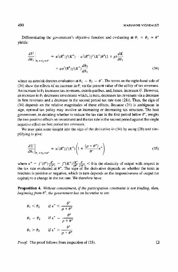
Differentiating the govemment's objective function and evaluating at 0t ---- 02 = 0*

yields:

dU o, dOt =02 =o*

dK = u'(R*)f(K*) + u'(R*)f'(K*)O*(1 + P)dot

, , , dO2 + pu ( R ) f ( K )~x; (34)

atlt

where an asterisk denotes evaluation at 0t = 02 = 0". The terms on the right-hand side of (34) show the effects of an increase in 0t on the present value of the utility of tax revenues. An increase in 0 t increases tax revenues, ceteris paribus, and, hence, increases U. However, an increase in 0 t decreases investment which, in turn, decreases tax revenues via a decrease in firm revenues and a decrease in the second period tax rate (see (28)). Thus, the sign of (34) depends on the relative magnitudes of these effects. Because (34) is ambiguous in sign, optimal tax policy may involve an increasing or decreasing tax structure. The host government, in deciding whether to reduce the tax rate in the first period below 0", weighs the two positive effects on investment and the tax rate in the second period against the single negative effect on first period tax revenues.

We may gain some insight into the sign of the derivative in (34) by using (28) and sim- plifying to give:

o, (1 (~ + dU = u'(R*)f(K*) + d O l =02=0 * O* ]

(35)

t * O* t * dK* O* where E* = f ( 0 ) ~ = f ( K ) ~ < 0 is the elasticity of output with respect to f(o*) the tax rate evaluated at 0". The sign ot tlae derivative depends on whether the term in brackets is positive or negative, which in turn depends on the responsiveness of output (or capital) to a change in the tax rate. We therefore have:

Proposition 4. Without commitment, if the participation constraint is not binding, then, beginning from 0", the government has an incentive to set:

- 0 " 01 < 0 2 i f e * < - -

p+O*

- - 0 " 01 = 02 if e* -

p+O*

- - 0 " 0 1 > 0 2 if e* > - -

p+O*

Proof" The proof follows from inspection of (35). []


Note that Proposition 4 does not depend on whether the government is able to borrow and lend. If the government is able to borrow and lend and has access to perfect capital markets, then u'(R*) = 1. Substituting this into (35) does not affect Proposition 4.

An elastic response implies that the government has an incentive to levy a tax rate in the first period such that 0~ - 02 = h(O~, 1-I2) so as not to induce a large reduction in investment. This result accords with that of the optimal tax literature, which prescribes an inverse relationship between the tax rate and elasticity, and is similar to a result obtained by Wen (1997). In Wen's model, an increasing tax rate arises because firms are able to adjust the capital stock in the second period, unlike in our model. Allowing capital to vary in the second period increases the elasticity of first period capital. Because of this, Wen obtains the result that 0~ < 02, reflecting the inverse relationship between the optimal tax rate and elasticity.

It is plausible, however, that the term in brackets in (35) is positive. In this case, the negative effects of taxation in the first period on investment are not large in comparison to the direct positive effect on tax revenues. Thus, the government can take advantage of an inelastic response to a change in the tax rate by choosing 01 such that 01 ---> 02 = h(01, 17~). It is this situation that yields results substantially different from those found in the literature.

One explanation for the divergence of our results with those in the literature is that, in the models employed by Doyle and van Wijnbergen (1994) and Bond and Samuelson (1986), the level of capital is determined exogenously and is, therefore, fixed in every period. This would suggest a decreasing tax rate in accordance with our Proposition 4 with a perfectly inelastic capital response. In their models, however, other factors establish the time structure of tax rates. In Doyle and van Wijnbergen, an increasing tax rate reflects the fact that successive bargaining reduces returns to foreign investment because the firm incurs addi- tional costs in terms of lost goodwill on the part of the government. In Bond and Samuelson, the fact that the capital stock is not allowed to vary implies that the host government can raise the tax rate in each of two periods to the level where the firm is indifferent between producing in the host country and leaving to produce in the home country. Because the value of the outside option of investing at home is greater in period 1 than it is in period 2, the maximum tax rate the host government can levy without driving the firm away is smaller in period 1 than in period 2. Another explanation for the divergence in results is incorporated in the model employed by Wen (1997). As was discussed above, in his model, the optimal tax rate is lower in period 1 than in period 2 because the firms are able to adjust the capital stock in the second period.

In the commitment case examined in Section 3, we found that the time structure of tax rates depends on the relative magnitudes of p and/3. In the non-commitment case examined here, the magnitudes of p and/3 affect the likelihood that the tax rate increases over time. For example, if the firms' participation constraint is not binding, we see from Proposition 4 that a higher p makes it more likely that 01 <~ 02. Also, /3 affects the elasticity term ~:* = f l ( l ( * , l d K * O* j , . . , ~ - f - ~ . A lower/3, ceteris paribus, reduces the level of capital chosen in

period 1. Thus, f'(K*) increases and f(O*) decreases, tending to increase ~*. However, a dK* lower/3, by decreasing K*, reduces 0* and has an ambiguous effect on ~ - , and can be

determined by differentiating dK* " o * and evaluatm~ at 0 .


(ii) Binding participation constraint. Recall that a necessary condition for this case is that H~ is sufficiently small relative to II*. If this condition holds, we have:

Proposition 5. Without commitment, the time structure of tax rates is non-decreasing if the participation constraint is binding at 0".

Proof" Let 01 be the unconstrained optimal tax rate for period 1. It is then clear that: (i) A constant tax rate arises if the participation constraint becomes binding at 01 = O* and 01 > O* and (ii) An increasing tax rate arises if the participation constraint becomes binding at 0t < 0". []

The intuition behind Proposition 5 is straightforward. We know from (28) that a decrease in 01 increases the level of capital. A higher level of capital relaxes the participation constraint in the second period and, as a result, implies a higher 02. Thus, lowering 01 from the unconstrained optimum to the level where the participation constraint binds increases 02. We must then have the result that 01 -< 0* --< 02. Also note that Proposition 5 does not depend on whether the host government is able to borrow and lend, since it refers to the firms' participation constraint and not the government's optimization problem.

From inspection of the participation constraint from the government's optimization problem (see (30) with (26)), it is clear that decreases in/3, increases in qK, and increases in II* increase the likelihood that the constraint binds. In addition, a decrease in FI~ decreases the firms' present value of profits and shifts the function 02 = h(O1, II~) upwards (see (29)), thus increasing 0* and increasing the likelihood that the constraint binds.

Note that this result corresponds to those obtained by Bond and Samuelson (1986) and Doyle and van Wijnbergen (1994). As described above, in their papers, capital is not allowed to vary in either period, implying that optimal tax policy will be such that the firms' participation constraint binds.

5. A comparison of commitment and non-commitment

We are now in a position to compare the commitment and non-commitment cases. In the analysis of the commitment case, we found that the relative magnitude of p and/3 determined the time structure of tax rates. In particular, the commonly observed structure of increasing tax rates arises if p > /3. Thus, p > /3 is sufficient for the tax rate to increase over time. In the non-commitment case, the relationship between the relative magnitude of p and/3 and the time structure of tax rates is not as strong. Specifically, p > / 3 is not sufficient for the tax rate to increase over time, but it does affect the likelihood of this occurring. We also found that two key elements in determining the time structure of tax rates in the non-commitment case are the relative values of the firms' outside options of investing in another country and the responsiveness of capital to a change in the tax rate.

The determinants of the time structure of tax rates are very different with commitment than without. The difference can be explained if we consider the type of strategy that is


available for each case. In the commitment case, the government chooses the time path of tax rates at the initial date, taking into consideration the response of the firms. The firms, in turn, choose the level of capital after having observed the choice of tax rates for both periods. No further decisions are taken. Consequently, the tax rate levied in period 2 will be a function only of time and not of the level of capital. Thus, only discount rates influence the time structure of taxes. By contrast, in the non-commitment case, the tax rate levied in period 2 is permitted to depend on the level of capital. The government chooses the tax rate for period 1 at the initial date, taking into consideration the response of the firms to the chosen tax rate, and selects a decision rule that specifies what tax rate will be levied in period 2 depending on the level of capital chosen in period 1. Thus, a key determinant of the optimal time structure for tax rates is the responsiveness of capital to a change in the tax rate.

6. Conclusion

This paper has investigated the role of commitment to future tax policy as an explanation for tax incentives in the form of rates that increase over time. A standard explanation for this type of tax incentive is that lack of commitment combined with irreversible investment allows host governments to levy increasing tax rates. Our principal result is that inability to commit to tax policy combined with fixed capital costs is neither sufficient nor necessary to generate an increasing tax structure. We found that, when the host government cannot commit to tax policy, the time structure of tax rates depends on the relative values of the finns' outside option of investing elsewhere in the world in period 1 relative to the value in period 2 and on the elasticity of capital with respect to the tax rate in period 1. If the value of the outside option in period 2 is not too small relative to period 1, then an elastic capital response gives rise to an increasing tax rate. Conversely, an inelastic capital response yields a decreasing tax rate. If, instead, the value of the outside option of investing elsewhere in period 2 is sufficiently small relative to period 1, then the tax rate is non-decreasing.

If the host government is able to commit to tax policy, we found that the optimal tax structure is sensitive to the rates at which the future is discounted by finns and governments. Specifically, an increasing tax structure may arise if factors are present that make the host government discount the future less than the firms do. Thus, we may observe increasing tax rates if, for example, the taxation of capital income yields a higher cost of finance than the after-tax return to savings or if there exist externalities in savings for bequests.

For our analysis, we employed a two-period model wherein firms choose a level of capital in the first period that remains fixed in the second period. An interesting exercise would be to expand the time horizon and allow ongoing investment, which would permit an analysis of the time paths and steady states of capital and the tax rate. Another interesting extension would endogenize the profits arising from the firms exercising their option to invest elsewhere in the world. To do this, one could incorporate the home country into the model by giving the firms the opportunity to invest at home and/or in the host country in response to endogenously determined tax rates in both countries. Or, a similar analysis could give


the firms the opportunity to invest in another host country with the tax treatment determined endogenously in both countries. Both of these scenarios would incorporate the possible in- terdependence and competition between countries with regard to the taxation of foreign direct investment.

Notes

1. For extensions of this idea, see Bond and Samuelson (1986, 1989), King and Welling (1992), and Wen (1997). 2. We make this assumption for convenience. Generalizing the number of firms to a constant n does not make any

qualitative difference to the results. 3. I am grateful to a referee for raising the issue of borrowing and lending. 4. This would be the case if, for example, there were many firms and many potential host countries leading to

a competitive equilibrium where profits are driven to zero. This result corresponds to and accords with that of Doyle and van Wijnbergen-(1994). Combining II~ = 0 with irreversible investment implies that the host government is able to tax away all profits without driving the firms out of the country.

5. The existence and uniqueness of 0* follows from the results 02(01, HI) ~ (0, 1) and ~ < 0. Thus, if we plot 02 against 0~, the function 02(0~, II~) intersects the 45-degree line only once where 0~ = 02 = 0* and 0* ~ (0, 1).

References

Alworth, J.S. (1988), The Finance, Investment and Taxation Decisions of Multinationals. Oxford: Basil Blackwell Ltd.

Bond, E.W. and L. Samuelson (1986), "Tax Holidays as Signals," American Economic Review, 76, 820-826. Bond, E.W. and L. Samuelson (1989), "Bargaining with Commitment, Choice of Techniques, and Direct Foreign

Investment," Journal of International Economics. 26, 77-97. Caves, R. (1982), Multinational Enterprise and Economic Analysis. New York: Cambridge University Press. Chari, V., P. Kehoe, and E. Prescott (1989), "Time Consistency and Policy," in R. Barro (ed.) Modern Business

Cycle Theory. Cambridge: Harvard University Press. Doyle, C. and S. van Wijnbergen (19~4), "Taxation of Foreign Multinationals: A Sequential Bargaining Approach

to Tax Holidays," International Tax and Public Finance, 1, 211-225. Eaton, J. and M. Gersovitz (1983), "Country Risk: Economic Aspects," in R.J. Herring (ed.) Managing Interna-

tional Risk. New York: Cambridge University Press. Feldstein, M.S. (1972), "The Social Time Preference Rate," in R. Layard (ed.) Cost-Benefit Analysis. London:

Penguin Books Inc. Fischer, S. (1980), "Dynamic Inconsistency, Cooperation and the Benevolent Dissembling Government," Journal

of Economic Dynamics and Control, 2, 93-107. King, I. and L. Welling (1992). "Commitment, Efficiency and Footloose Firms," Economica, 59, 63-73. Kydland, EE. and E.D. Prescott (1977), "Rules Rather than Discretion: The Inconsistency of Optimal Plans,"

Journal of Political Economy, 85,473-491. Marglin, S.A. (1963), "The Social Rate of Discount and the Optimal Rate of Investment," Quarterly Journal of

Economics, 77, 95-112. Sen, A.K. (1961), "On Optimizing the Rate of Saving," Economic Journal, 77,479-96. Wen, J. (1992), "Tax Holidays in a Business Climate," Queen's University Working Paper No. 864.

commitment and the time structure of taxation of foreign direct investment

Documents