comments on an introduction of the gpm model · comments on an introduction of the gpm model by...
TRANSCRIPT

Comments onAn Introduction of the GPM Model
by Michel Juillard
Mototsugu Shintani1
1RCASTUniversity of Tokyo
7th Annual ESRI-CEPREMAP Joint Workshop 2014November 13, 2014

What is GPM?
I GPM is the Global Projection Model developed by theresearch sta¤ of IMF.
I GPM is designed to be a common basis for central bankers
1. to generate forecast in multi-country framework
2. to conduct policy analysis in multi-country framework
I GPM is not
1. a DSGE model
2. a VAR model (or other atheoretical time-series models)
but is something in-between
I GPM is not
1. a fully calibrated model
2. a purely estimated model
but is something in-between

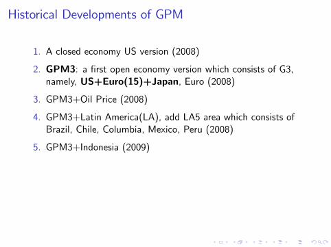
Historical Developments of GPM
1. A closed economy US version (2008)
2. GPM3: a �rst open economy version which consists of G3,namely, US+Euro(15)+Japan, Euro (2008)
3. GPM3+Oil Price (2008)
4. GPM3+Latin America(LA), add LA5 area which consists ofBrazil, Chile, Columbia, Mexico, Peru (2008)
5. GPM3+Indonesia (2009)
6. GPM6: Total of 6 areas, G3+Emerging Asia(EA10, includesChina)+Latin America(LA5)+Remaining Countries(RC17,includes Russia, UK, Canada) (2013)
7. GPM7: GPM6+China (2013)

Notable Features of GPM
I Use Bayesian methods to estimate (a part of) unknownparameters in the model.
I The user (central bankers) can customize the model by addingindividual country to basic GPM3 (or GPM6).
I Financial-real linkages are captured by a single �nancialvariable called BLT.
I a US bank lending tightening (BLT) measure constructed fromloan o¢ cer opinion survey (+ tightening - easing).
I Equilibrium level (e.g., Y) is I(1), its increment (steadygrowth) has both a persistence component and an iidcomponent.
I Core of the model consists of (i) output gap equation, (ii)Phillips curve, (iii) Taylor rule, and (iv) UIP, with equilibriaY,U,Z, being I(1).

Question 1: Sequential Bayesian Estimation?I Mixture of calibrated parameters and estimated parameters inDSGE modeling is not uncommon ! �xed parametercorresponds to prior with mass point.
I Because the baseline model was GPM3, it is not desirable ifthe original parameters of G3 part change dramatically byadding new countries.
I To handle this problem, GPM6 employs the followingsequential procedure:
1. GPM3 estimated using the mixture of calibrated parameters and estimatedparameters.
2. Treat all the parameters as �xed, and add a region one by one and estimate theGPM3+1 region using the mixture of calibrated parameters and estimatedparameters.
3. Repeat this for all regions to obtain GPM6 or GPM7.
I This is di¤erent from the timing of arrival of newobservations, or Bayesian updating. Is there theoreticaljusti�cation? How to interpret the marginal data density?

Table 1 from Carabenciov et al. (2013) GPM647
GPM6 Parameters 1
US Euro Area Japan EA6 LA6 RC6
Steady State ValuesGDP Growth 2.273 2.261 1.444 7.900 4.000 4.000Real Interest Rate 1.728 1.984 1.379 2.000 2.000 2.000Inflation Target 2.500 1.900 1.000 4.000 3.500 4.500
Adjustment Coefficientsτ Potential Output 0.027 0.029 0.037 0.030 0.030 0.030ρ Real Interest Rate 0.290 0.467 0.030 0.200 0.200 0.200χ Real Exchange Rate 0.050 0.050 0.050
Output Gapβ1 Lag 0.569 0.756 0.779 0.471 0.544 0.441β2 Lead 0.231 0.044 0.021 0.215 0.178 0.408β3 Medium-term interest rate gap 0.187 0.201 0.148 0.200 0.200 0.200β4 REER gap 0.051 0.067 0.036 0.171 0.148 0.070β5 Foreign Activity 0.891 0.891 0.891 0.891 0.891 0.891θ BLT 1.071 0.300 0.300 0.996 0.992 0.996
Headline Inflationλ1 Lead 0.750 0.700 0.750 0.720 0.594 0.545λ2 Output gap 0.180 0.222 0.184 0.197 0.228 0.149λ3 REER gap 0.100 0.246 0.152 0.081 0.161 0.098
Monetary Policy Ruleγ1 Lag 0.711 0.686 0.750 0.667 0.645 0.725γ2 Inflation gap 0.910 1.306 1.058 1.114 0.911 0.898γ4 Output gap 0.205 0.201 0.169 0.169 0.202 0.162
UIPφ Exp Change in Exch Rate 0.834 0.856 0.800 0.800 0.800
Unemployment Dynamic Okun’s Lawα1 Lag 0.824 0.717 0.759α2 Output gap 0.182 0.140 0.060(1-α3) Trend coefficient 0.635 0.899 0.779
Med-Term Interest Rate Weightsξ1 1 qtr ahead 0.100 0.100 0.100 0.100 0.100 0.100ξ4 1 yr ahead 0.350 0.350 0.350 0.350 0.350 0.350ξ12 3 yrs ahead 0.350 0.350 0.350 0.350 0.350 0.350ξ20 5 yrs ahead 0.200 0.200 0.200 0.200 0.200 0.200
1 Estimated parameters are in green. Partially estimated (GPM3 or GPM4) are in red. Calibrated parameters arein black.
Table 1. GPM6 Parameters TableEstimated parameters are in green. Partially estimated (GPM3 orGPM4) are in red. Calibrated parameters are in black.

Question 1: Sequential Bayesian Estimation?I Mixture of calibrated parameters and estimated parameters inDSGE modeling is not uncommon ! �xed parametercorresponds to prior with mass point.
I Because the baseline model was GPM3, it is not desirable ifthe original parameters of G3 part change dramatically byadding new countries.
I To handle this problem, GPM6 employs the followingsequential procedure:
1. GPM3 estimated using the mixture of calibrated parameters and estimatedparameters.
2. Treat all the parameters as �xed, and add a region one by one and estimate theGPM3+1 region using the mixture of calibrated parameters and estimatedparameters.
3. Repeat this for all regions to obtain GPM6 or GPM7.
I This is di¤erent from the timing of arrival of newobservations, or Bayesian updating. Is there theoreticaljusti�cation? How to interpret the marginal data density?

Question 2: Forecasting Exercise?
I In the evaluation of an estimated DSGE model, its forecastingperformance is often evaluated in comparison to (Bayesian)VAR forecasts. Out-of-sample forecasts of the DSGE modelcan be obtained from the RE solution (policy function) sinceall the variables are in lags.
I In GPM, not only lagged variables but also lead variables areincluded to �allow more complex dynamics and forward-lookingelements in aggregate demand (Carabenciov et al., 2008).�
yt = β1yt�1 + β2yt+1 + ...+ εyt
I Unconditional forecast? Conditional forecast using judgmentalprojection of the exogenous variables and the tuning ofendogenous variables?
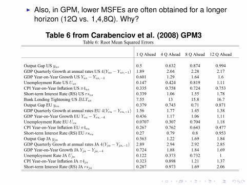
I Also, in GPM, lower MSFEs are often obtained for a longerhorizon (12Q vs. 1,4,8Q). Why?
Table 6 from Carabenciov et al. (2008) GPM3
40
Table 6: Root Mean Squared Errors
1 Q Ahead 4 Q Ahead 8 Q Ahead 12 Q Ahead
Output Gap US yus 0.5 0.632 0.874 0.994GDP Quarterly Growth at annual rates US 4(Yus � Yus;�1) 1.89 2.04 2.28 2.17GDP Year-on-Year Growth US Yus � Yus;�4 0.601 1.29 1.64 1.6Unemployment Rate US Uus 0.147 0.424 0.819 1.11CPI Year-on-Year In�ation US �4us 0.335 0.758 0.724 0.753Short-term Interest Rate (RS) US rsus 0.339 1.06 1.55 1.78Bank Lending Tightening US BLTus 7.55 13 15.8 16.7Output Gap EU yeu 0.379 0.743 0.71 0.871GDP Quarterly Growth at annual rates EU 4(Yeu � Yeu;�1) 1.56 1.77 1.45 1.38GDP Year-on-Year Growth EU Yeu � Yeu;�4 0.436 1.17 1.06 1.11Unemployment Rate EU Ueu 0.0707 0.307 0.704 1.18CPI Year-on-Year In�ation EU �4eu 0.267 0.762 0.643 0.477Short-term Interest Rate (RS) EU rseu 0.27 0.79 0.8 0.953Output Gap JA yja 0.563 1.22 1.69 1.84GDP Quarterly Growth at annual rates JA 4(Yja � Yja;�1) 2.89 2.94 2.92 2.85GDP Year-on-Year Growth JA Yja � Yja;�4 0.724 1.88 1.84 1.69Unemployment Rate JA Uja 0.122 0.373 0.732 1CPI Year-on-Year In�ation JA �4ja 0.323 0.898 1.21 1.37Short-term Interest Rate (RS) JA rsja 0.287 0.973 1.69 2.06

Question 3: Stochastic Trend in RER?
I In GPM6, real exchange rate (RER) of emerging marketeconomies contains trends of appreciation to captureBalassa-Samuelson e¤ect.
I But G3 also has stochastic trend in equilibrium RER as
Zt = Zt�1 + εzt
where Zt is the equilibrium RER so that RER is I(1).
I Linear trend dominates stochastic trend so rate of divergenceis faster for emerging market, but still diverging. What isbehind the divergence of RER among G3?