comm-02-fourier theory and communication signals

Chapter2Chapter2Chapter2Chapter2Fourier Theory and Communication Fourier Theory and Communication

SignalsSignals

Wireless Information Transmission System Lab.Wireless Information Transmission System Lab.Institute of Communications EngineeringInstitute of Communications Engineeringg gg gNational Sun National Sun YatYat--sensen UniversityUniversity

ContentsContents

◊ 2.1 Introduction2 2 The Fo rier Transform◊ 2.2 The Fourier Transform

◊ 2.3 Properties of The Fourier Transform◊ 2 4 The Inverse Relationship between Time and Frequency◊ 2.4 The Inverse Relationship between Time and Frequency◊ 2.5 Dirac Delta Function◊ 2.6 Fourier Transform of Periodic Signals◊ 2.6 Fourier Transform of Periodic Signals◊ 2.7 Transmission of Signals Through Linear Systems◊ 2.8 Filters◊ 2.9 Low-Pass and Band-Pass Signals◊ 2.10 Band-Pass Systems◊ 2.11 Phase and Group Delay◊ 2.12 Sources of Information

2

◊ 2.13 Numerical Computation of the Fourier Transform

Chapter 2.1Chapter 2.1IntroductionIntroductionIntroductionIntroduction


Chapter 2.1 IntroductionChapter 2.1 Introductionpp

◊ We identify deterministic signals as a class of signals whose f d fi d tl f ti f tiwaveforms are defined exactly as functions of time.

◊ In this chapter we study the mathematical description of such◊ In this chapter we study the mathematical description of such signals using the Fourier transform that provides the link between the time-domain and frequency-domain descriptions of signal.

A h l d i h d i hi h i h◊ Another related issue that we study in this chapter is the representation of linear time-invariant systems. Filters of different kinds and certain communication channels are important examples of this class of systems.

4

Chapter 2.2Chapter 2.2The Fourier TransformThe Fourier TransformThe Fourier TransformThe Fourier Transform


Chapter 2.2 The Fourier TransformChapter 2.2 The Fourier Transform

◊ Fourier transform is defined as

( ) ( ) ( )exp 2G f g t j ft dtπ∞

−∞= −∫

◊ g(t) denote a nonperiodic deterministic signal.◊ .1j = −◊ variable f denotes frequency and t denotes time.

◊ Inverse Fourier transform is defined as

( ) ( ) ( )exp 2g t G f j ft dfπ∞

−∞= ∫

6


◊ We have used a lowercase letter to denote the time function and a uppercase letter to denote the corresponding frequency function Theuppercase letter to denote the corresponding frequency function. The functions g(t) and G( f ) are said to constitute a Fourier-transform pair.

◊ For the Fourier transform of a signal g(t) to exist, it is sufficient, but not necessary, that g(t) satisfies three sufficient conditions known collectively as Dirichlet’s conditions:◊ The function g(t) is single-valued, with a finite number of

i d i i i fi it ti i t lmaxima and minima in any finite time interval.◊ The function g(t) has finite number of discontinuities in any finite

time intervaltime interval.◊ The function g(t) is absolutely integrable, i.e.

7

( )g t dt∞

−∞< ∞∫


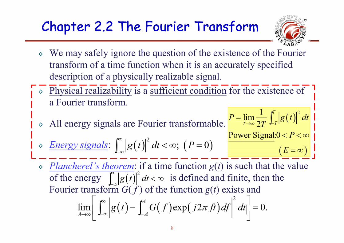
◊ We may safely ignore the question of the existence of the Fourier transform of a time function when it is an accurately specifiedtransform of a time function when it is an accurately specified description of a physically realizable signal.

◊ Physical realizability is a sufficient condition for the existence of y ya Fourier transform.

All i l F i t f bl ( ) 21lim2

T

TP g t dt

T= ∫◊ All energy signals are Fourier transformable.

◊ Energy signals: ( ) ( )2; 0g t dt P

∞< ∞ =∫

( )

( )

2Power Signal:0

TTg

TP

E

−→∞

< < ∞

∞

∫

gy g

◊ Plancherel’s theorem: if a time function g(t) is such that the value of the energy is defined and finite then the( ) 2

t dt∞

<∫

( ) ( );g−∞∫ ( ) E = ∞

of the energy is defined and finite, then the Fourier transform G( f ) of the function g(t) exists and

( )g t dt−∞

< ∞∫

( ) ( ) ( )2

li 2 0A

G f j f df d∞⎡ ⎤∫ ∫

8

( ) ( ) ( )lim exp 2 0.AA

g t G f j ft df dtπ−∞ −→∞

⎡ ⎤− =⎢ ⎥

⎣ ⎦∫ ∫


◊ Notations◊ time t measured in second (s)◊ time t measured in second (s)◊ frequency f measured in Hertz (Hz)

l f (radians per second rad/s)2 f◊ angular frequency (radians per second, rad/s).◊ A convenient shorthand notation for the transform relations:

F i t f ti

2 fω π=

◊ Fourier transformation

( ) ( )G f F g t⎡ ⎤= ⎣ ⎦◊ Inverse Fourier transformation

( ) ( )⎣ ⎦

( ) ( )1t F G f− ⎡ ⎤⎣ ⎦

where and play the roles of linear operators.

( ) ( )1g t F G f⎡ ⎤= ⎣ ⎦

[ ]1F −[ ]F

9

◊ Fourier-transform pair ( ) ( )g t G f


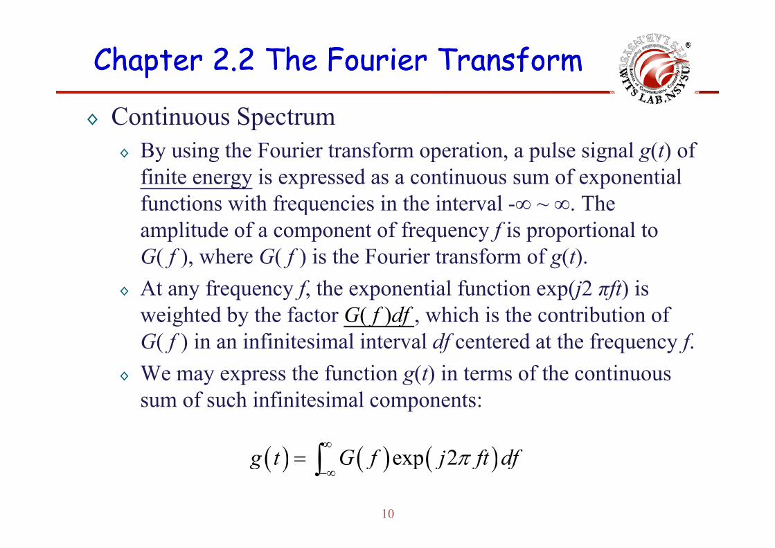
◊ Continuous Spectrum◊ By using the Fourier transform operation a pulse signal g(t) of◊ By using the Fourier transform operation, a pulse signal g(t) of

finite energy is expressed as a continuous sum of exponential functions with frequencies in the interval -∞ ~ ∞. The qamplitude of a component of frequency f is proportional to G( f ), where G( f ) is the Fourier transform of g(t).

◊ At any frequency f, the exponential function exp(j2 πft) is weighted by the factor G( f )df , which is the contribution of G( f ) i i fi it i l i t l df t d t th f fG( f ) in an infinitesimal interval df centered at the frequency f.

◊ We may express the function g(t) in terms of the continuous sum of such infinitesimal components:sum of such infinitesimal components:

( ) ( ) ( )exp 2g t G f j ft dfπ∞

= ∫10

( ) ( ) ( )exp 2g t G f j ft dfπ−∞

= ∫


◊ In general, the Fourier transform G( f ) is a complex function of frequency f : ( ) ( ) ( )⎡ ⎤frequency f : ( ) ( ) ( )expG f G f j fθ⎡ ⎤= ⎣ ⎦

( ) ( ) is called the continuous amplitude spectrum of G f g t( ) ( )( ) ( )

p p

is called the continuous phase spectrum of

f g

f g tθ

◊ If g(t) is a real-valued function of t, then◊ G( f )=G*( f )

( ) ( )

( ) ( )( )2

*2

j ft

j f

G f g t e dtπ∞ −

−∞

∞

= ∫

∫◊ G(-f )=G*( f )◊ |G(-f )|=|G( f )|: an even function of fΘ( f )= Θ( f ): an odd function of f

( ) ( )( )( )

( )

2

2

* j ft

j ft

G f g t e dt

g t e dt

G f

π

π

∞ −

−∞

∞

−∞

=

=

∫

∫◊ Θ(-f )=-Θ( f ): an odd function of f◊ The spectrum of a real-valued signal exhibits conjugate symmetry.

( )G f= −

11


◊ [Example 2.1] Rectangular Pulse◊ Define a rectangular function of unit amplitude and unit◊ Define a rectangular function of unit amplitude and unit

duration:( )

1 11,2 2rect

tt

⎧ − < <⎪⎪= ⎨( )rect10,2

tt

⎨⎪ ≥⎪⎩

t⎛ ⎞ ( )t⎛ ⎞

Real-Valuedand Symmetric

( ) rect tg t AT⎛ ⎞= ⎜ ⎟⎝ ⎠

( ) ( )/2

/2exp 2

T

TG f A j ft dtπ= −∫

( )rect sinctA AT fTT⎛ ⎞⎜ ⎟⎝ ⎠

(2.10)

( )

( )

/2

/2

/2cos(2 ) sin(2 )

i

T

T

T

T

A ft j ft dt

f

π π

−

−= −

∫∫

( )

( )

2/2

00

sin 22 cos(2 ) 2

2

sin

T ftA ft dt A

f

fT

ππ

π

π

= =

⎛ ⎞

∫

( )i λ

Real-Valuedand Symmetric

12

( ) ( )sinsinc

fTAT AT fT

fTπ

π⎛ ⎞

= ≡⎜ ⎟⎝ ⎠

( ) ( )sinsinc

πλλ

πλ≡

Chapter 2.2 The Fourier TransformChapter 2.2 The Fourier Transform◊ sinc function

( ) ( )sinsinc

πλλ ≡( ) ( )

sinc λπλ

≡

◊ As the pulse duration T is decreased the first zero crossing of the◊ As the pulse duration T is decreased, the first zero-crossing of the amplitude spectrum |G( f )| moves up in frequency.

◊ The relationship between the time-domain and frequency-domain is◊ The relationship between the time domain and frequency domain is an inverse one.

◊ A pulse, narrow in time, has a significant frequency description over

13

◊ A pulse, narrow in time, has a significant frequency description over a wide range of frequencies, and vice versa.


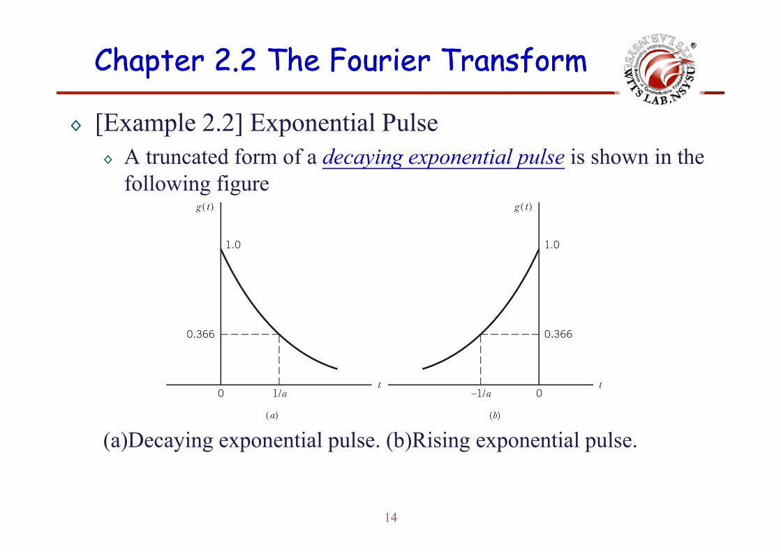
◊ [Example 2.2] Exponential PulseA t t d f f d i i l l i h i th◊ A truncated form of a decaying exponential pulse is shown in the following figure

(a)Decaying exponential pulse. (b)Rising exponential pulse.

14


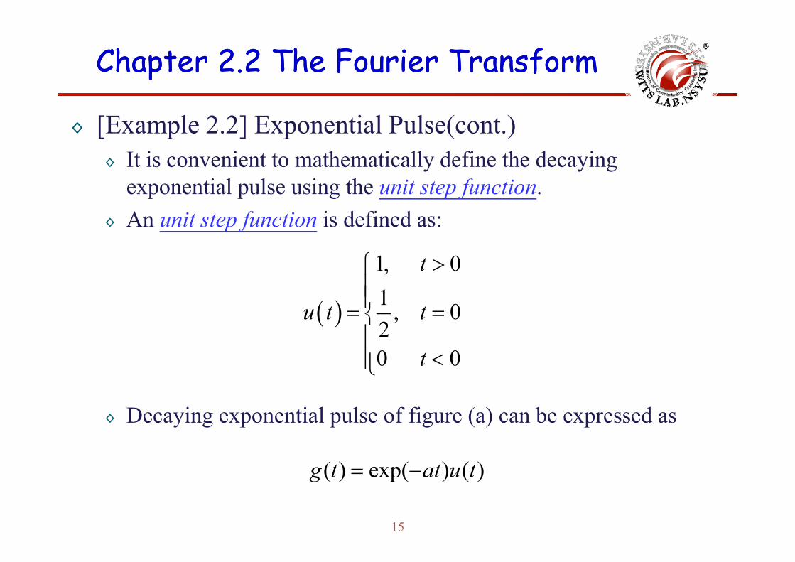
◊ [Example 2.2] Exponential Pulse(cont.)It i i t t th ti ll d fi th d i◊ It is convenient to mathematically define the decaying exponential pulse using the unit step function.An unit step function is defined as:◊ An unit step function is defined as:

1, 0t >⎧⎪

( ) 1 , 02

u t t⎪⎪= =⎨⎪

D i i l l f fi ( ) b d

0 0t⎪

<⎪⎩

◊ Decaying exponential pulse of figure (a) can be expressed as

( ) exp( ) ( )g t at u t= −

15

( ) exp( ) ( )g t at u t=


the Fourier transform of this pulse is

( ) ( ) ( )2G f t j ft dt∞

∫( ) ( ) ( )

( )( )

0exp exp 2

exp 2

G f at j ft dt

t a j f

π

π∞

∞

= − −

⎡ ⎤− +⎣ ⎦⎡ ⎤

∫

∫ ( )( )

( )00

e pexp 2

2

1

t a j ft a j f dt

a j fπ

ππ

∞ ⎡ ⎤⎣ ⎦⎡ ⎤= − + = −⎣ ⎦ +∫12a j fπ

=+

the Fourier-transform pair for the decaying exponential pulse of figure (a) is thereforefigure (a) is therefore

( ) ( ) 1exp at u t−

16

( ) ( )exp2

at u ta j fπ+


◊ [Example 2.2] Exponential Pulse(cont.)Ri i ti l l f Fi (b)◊ Rising exponential pulse of Fig. (b)

( ) ( ) ( )expg t at u t= − ( ) ( ) 1exp2

at u tj f

−( ) ( ) ( )

( ) ( ) ( )0

exp exp 2G f at j ft dtπ−∞

= −∫

( ) ( )p2a j fπ−

( )0 1exp 2

2t a j f dt

a j fπ

π−∞⎡ ⎤= − =⎣ ⎦ −∫

◊ The decaying and rising exponential pulses are both asymmetric functions of time t .Th i F i f h f l l d◊ Their Fourier transforms are therefore complex valued.

◊ Truncated decaying and rising exponential pulses have the same amplitude spectrum but the phase spectrum of the one is

17

same amplitude spectrum, but the phase spectrum of the one is the negative of that of the other.

FourierFourier--transform Pairstransform Pairs

18

Chapter 2.3Chapter 2.3Properties of The Fourier Properties of The Fourier pp

TransformTransform


Chapter 2.3 Properties of the Fourier Transform Chapter 2.3 Properties of the Fourier Transform

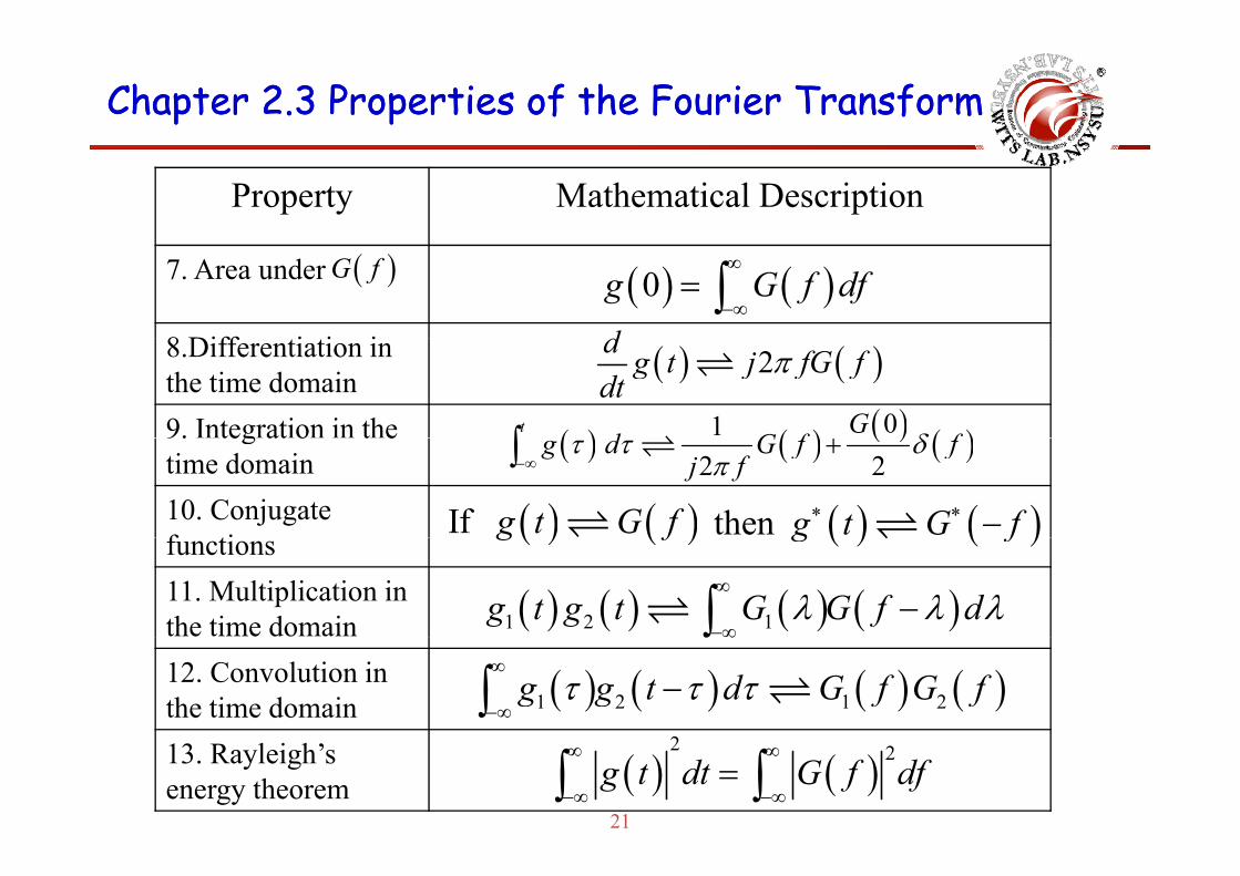
◊ Summary of properties of the Fourier transform

Property Mathematical Description

1 Linearity ( ) ( ) ( ) ( )1 2 1 2 ,ag t bg t aG f bG f+ +1. Linearity

2. Time scaling

( ) ( ) ( ) ( )1 2 1 2 , and are constants.

ag t bg t aG f bG fa b

+ +

( ) 1 fg at G ⎛ ⎞⎜ ⎟⎝ ⎠ where is constantag

3. Duality

( )ga a⎜ ⎟

⎝ ⎠ where is constanta

( ) ( ) ( ) ( )If then g t G f G t g f−

4. Time shifting ( ) ( ) ( )0 0exp 2g t t G f j ftπ− −

5. Frequency shifting

6 A d ( )

( ) ( ) ( )exp 2 c cj f t g t G f fπ −

∞

∫20

6. Area under g(t) ( ) ( )0g t dt G∞

−∞=∫


Property Mathematical Description

7. Area under

8 Diff i i i

( )G f ( ) ( )0g G f df∞

−∞= ∫

d8.Differentiation inthe time domain9. Integration in the

( ) ( )2d g t j fG fdt

π

( ) ( ) ( ) ( )01t Gd G f fδ∫9. teg at o t e

time domain10. Conjugate f ti

( ) ( ) ( ) ( )2 2

g d G f fj f

τ τ δπ−∞

+∫

( ) ( )If g t G f ( ) ( )then g t G f∗ ∗ −functions11. Multiplication in the time domain

( ) ( )g f ( ) ( )g f

( ) ( ) ( ) ( )1 2 1g t g t G G f dλ λ λ∞

−∞−∫

12. Convolution in the time domain

∞∫( ) ( ) ( ) ( )1 2 1 2g g t d G f G fτ τ τ

∞

−∞−∫2

21

13. Rayleigh’s energy theorem ( ) ( )

2 2g t dt G f df

∞ ∞

−∞ −∞=∫ ∫


◊ Property 1：Linearity (Superposition)L t d Th f ll t t( ) ( )t G f ( ) ( )t G fLet and . Then for all constants c1and c2, we have

1 1( ) ( )g t G f 2 2( ) ( )g t G f

( ) ( ) ( )1 1 2 2 1 1 2 2c g t c g t c G c G f+ +

◊ Proof: the proof of this property follows simply from the linearity of the integrals defining G( f ) and g(t).

22


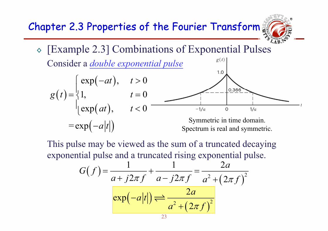
◊ [Example 2.3] Combinations of Exponential PulsesConsider a double exponential pulseConsider a double exponential pulse

( )exp , 0at t⎧ − >⎪( )

( )1, 0exp , 0

g t tat t

⎪= =⎨⎪ <⎩

Thi l b i d th f t t d d i

( ) =exp a t−Symmetric in time domain.

Spectrum is real and symmetric.

This pulse may be viewed as the sum of a truncated decaying exponential pulse and a truncated rising exponential pulse.

( ) 1 1 2aG f( )( )222 2 2

G fa j f a j f a fπ π π

= + =+ − +

( ) 2a

23

( )( )22

2exp2aa t

a fπ−

+


◊ [Example 2.3] Combinations of Exponential Pulses(cont.)

( )( )exp , 0

0 0at t

g t t⎧ − >⎪⎨( )

( )0, 0

exp , 0g t t

at t= =⎨⎪− <⎩

1, 0t+ >⎧⎪( )sgn 0, 0

1, 0t t

t

⎪= =⎨⎪− <⎩⎩

( ) ( ) ( )24

( ) ( ) ( )exp sgng t a t t= −


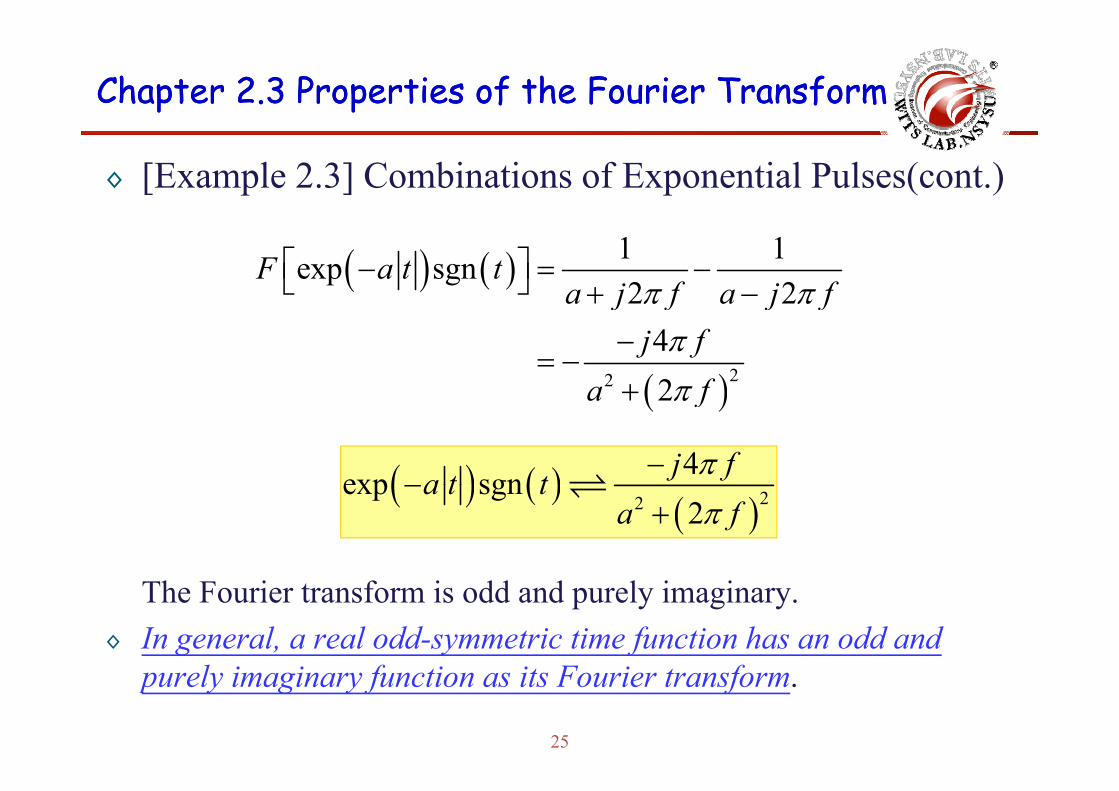
◊ [Example 2.3] Combinations of Exponential Pulses(cont.)

( ) ( ) 1 1exp sgn2 2

F a t ta j f a j fπ π

⎡ ⎤− = −⎣ ⎦ + −

( )22

42

j f j fj f

a fππ

−= −

+ ( )2a fπ+

( ) ( ) 4exp sgn j fa t t π−−( ) ( )

( )22exp sgn

2a t t

a fπ−

+

The Fourier transform is odd and purely imaginary.◊ In general, a real odd-symmetric time function has an odd and

l f f

25

purely imaginary function as its Fourier transform.


◊ Property 2：Time Scaling⎛ ⎞

Compression of a function inthe time domain is equivalent

Let . Then ( ) ( )g t G f ( ) 1 fg at Ga a

⎛ ⎞⎜ ⎟⎝ ⎠

the time domain is equivalent to the expansion of its Fourier

transform in the frequencydomain, or vice versa.

◊ Proof： ( ) ( ) ( )exp 2F g at g at j ft dtπ∞

−∞⎡ ⎤ = −⎣ ⎦ ∫ at t

aττ = → =

( ) ( )1 1For 0 : exp 2 f fa F g at g j d Ga a a a

τ π τ τ∞

−∞

⎡ ⎤⎛ ⎞ ⎛ ⎞⎡ ⎤> = − =⎜ ⎟ ⎜ ⎟⎢ ⎥⎣ ⎦ ⎝ ⎠ ⎝ ⎠⎣ ⎦∫

( ) ( )1For 0 : exp 2 fa F g at g j da a

τ π τ τ−∞

∞

⎡ ⎤⎛ ⎞⎡ ⎤< = − ⎜ ⎟⎢ ⎥⎣ ⎦ ⎝ ⎠⎣ ⎦∫

( )1 1 exp 2

a a

f fg j d Ga a a a

τ π τ τ∞

∞

⎝ ⎠⎣ ⎦⎡ ⎤⎛ ⎞ ⎛ ⎞= − − = −⎜ ⎟ ⎜ ⎟⎢ ⎥⎝ ⎠ ⎝ ⎠⎣ ⎦

∫

26

a a a a−∞ ⎢ ⎥⎝ ⎠ ⎝ ⎠⎣ ⎦∫

Q.E.D.


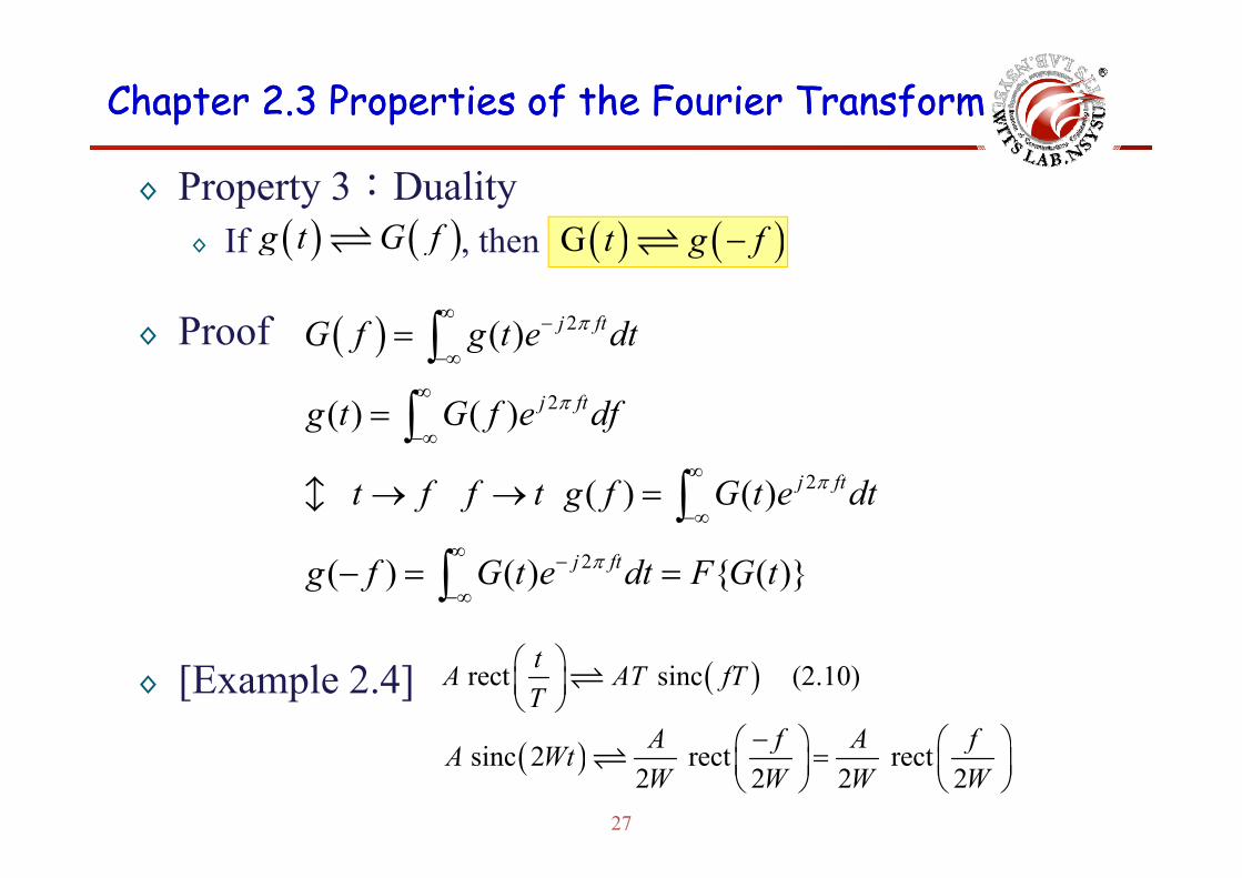
◊ Property 3：Duality◊ If then( ) ( )g t G f ( ) ( )G t g f◊ If , then

◊ Proof

( ) ( )g t G f ( ) ( )G t g f−

( ) 2( ) j ftG f g t e dtπ∞ −= ∫◊ Proof ( )2

( )

( ) ( ) j ft

G f g t e dt

g t G f e dfπ

−∞

∞

−∞

=

=

∫∫

2 ( ) ( ) j ftt f f t g f G t e dtπ

−∞

∞

−∞→ → =

∫∫

2( ) ( ) { ( )}j ftg f G t e dt F G tπ∞ −

−∞− = =∫

◊ [Example 2.4] ( )rect sinc (2.10)tA AT fTT⎛ ⎞⎜ ⎟⎝ ⎠

A f A f⎛ ⎞ ⎛ ⎞

27

( ) sinc 2 rect rect2 2 2 2A f A fA WtW W W W

−⎛ ⎞ ⎛ ⎞=⎜ ⎟ ⎜ ⎟⎝ ⎠ ⎝ ⎠


◊ Property 4：Time Shifting

◊ If , then( ) ( ) g t G f ( ) ( ) ( )0 0exp 2g t t G f j ftπ− −

◊ Proof ： ( )0Let t tτ = −

( ) ( ) ( )

( ) ( ) ( )

0 0 exp 2F g t t g t t j ft dtπ∞

−∞

∞

⎡ ⎤− = − −⎣ ⎦ ∫∫( ) ( ) ( )

( ) ( )0

0

exp 2 exp 2

exp 2

j ft g j f d

j ft G f

π τ π τ τ

π−∞

= − −

= −

∫

◊ The amplitude of G( f ) is unaffected by the time shift, but

( ) ( )0p j f f

28

its phase is changed by the linear factor -2πft0.


◊ Property 5：Frequency Shifting (Modulation Theorem)

◊ If , thenwhere is a real constant

( ) ( ) g t G f ( ) ( ) ( )exp 2 c cj f t g t G f fπ −fwhere is a real constant

◊ Proof：cf

( ) ( ) ( ) ( )exp 2 exp 2 c cF j f t g t g t j t f f dtπ π∞

∞⎡ ⎤ ⎡ ⎤= − −⎣ ⎦ ⎣ ⎦∫( ) ( ) ( ) ( )

( )cG f f−∞⎣ ⎦ ⎣ ⎦

= −

∫

◊ Multiplication of a function by the factor exp(-2πfct) is equivalent to shifting its Fourier transform in the positive q g pdirection by the amount fc.

29


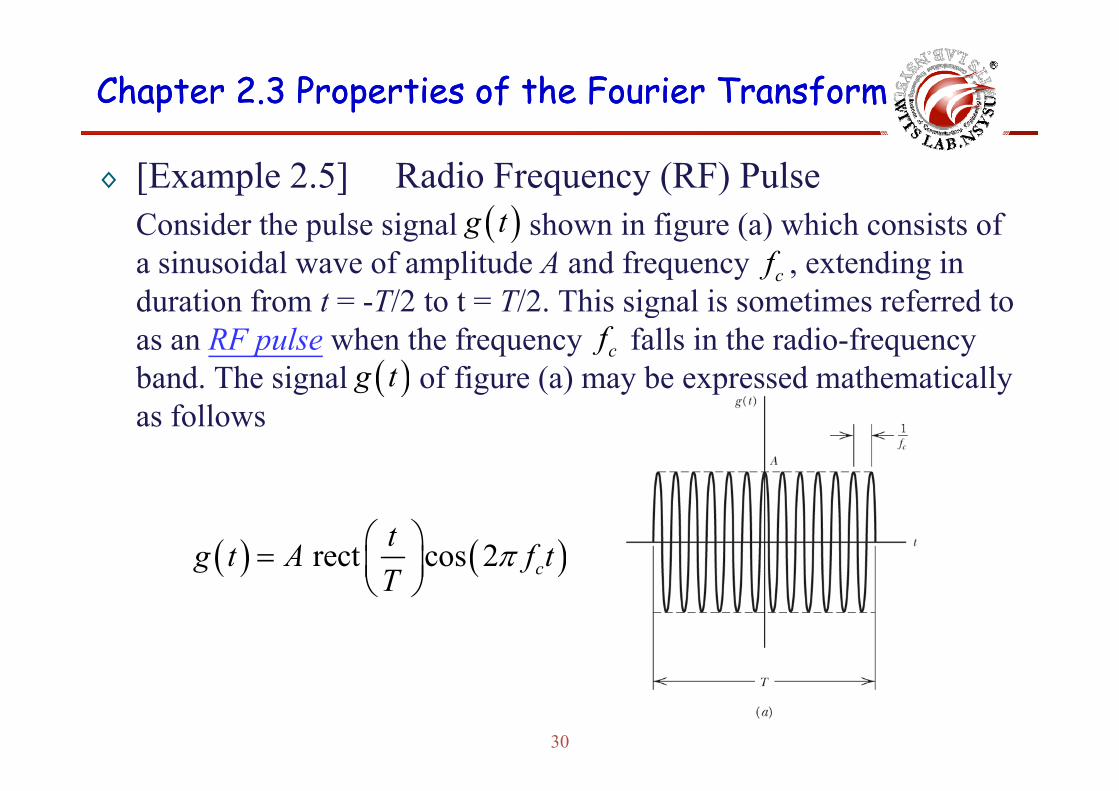
◊ [Example 2.5] Radio Frequency (RF) PulseC id th l i l h i fi ( ) hi h i t f( )tConsider the pulse signal shown in figure (a) which consists of a sinusoidal wave of amplitude A and frequency , extending in duration from t = -T/2 to t = T/2 This signal is sometimes referred to

( )g tcf

duration from t T/2 to t T/2. This signal is sometimes referred to as an RF pulse when the frequency falls in the radio-frequency band. The signal of figure (a) may be expressed mathematically

cf( )g t

as follows( )

( ) ( ) rect cos 2 ctg t A f tT

π⎛ ⎞= ⎜ ⎟⎝ ⎠

( ) ( )T⎜ ⎟⎝ ⎠

30


◊ [Example 2.5] Radio Frequency (RF) Pulse (cont.)we note thatwe note that

applying the frequency shifting property to the Fourier transform( ) ( ) ( )1cos 2 exp 2 exp 2

2c c cf t j f t j f tπ π π⎡ ⎤= + −⎣ ⎦applying the frequency-shifting property to the Fourier-transform pair, we get the desired result

( ) ( ) ( ){ }AT⎡ ⎤ ⎡ ⎤

in the special case of f T>>1 we may use the approximate result

( ) ( ) ( ){ }sinc sinc2 c c

ATG f T f f T f f⎡ ⎤ ⎡ ⎤= − + +⎣ ⎦ ⎣ ⎦

in the special case of fcT>>1, we may use the approximate result

( )sinc , 02 c

AT T f f f⎧ ⎡ ⎤− >⎣ ⎦⎪

( )

( )2

0, 0G f fAT

⎣ ⎦⎪⎪

=⎨⎪

31

( )sinc , 02 c

AT T f f f⎪

⎡ ⎤⎪ + <⎣ ⎦⎩


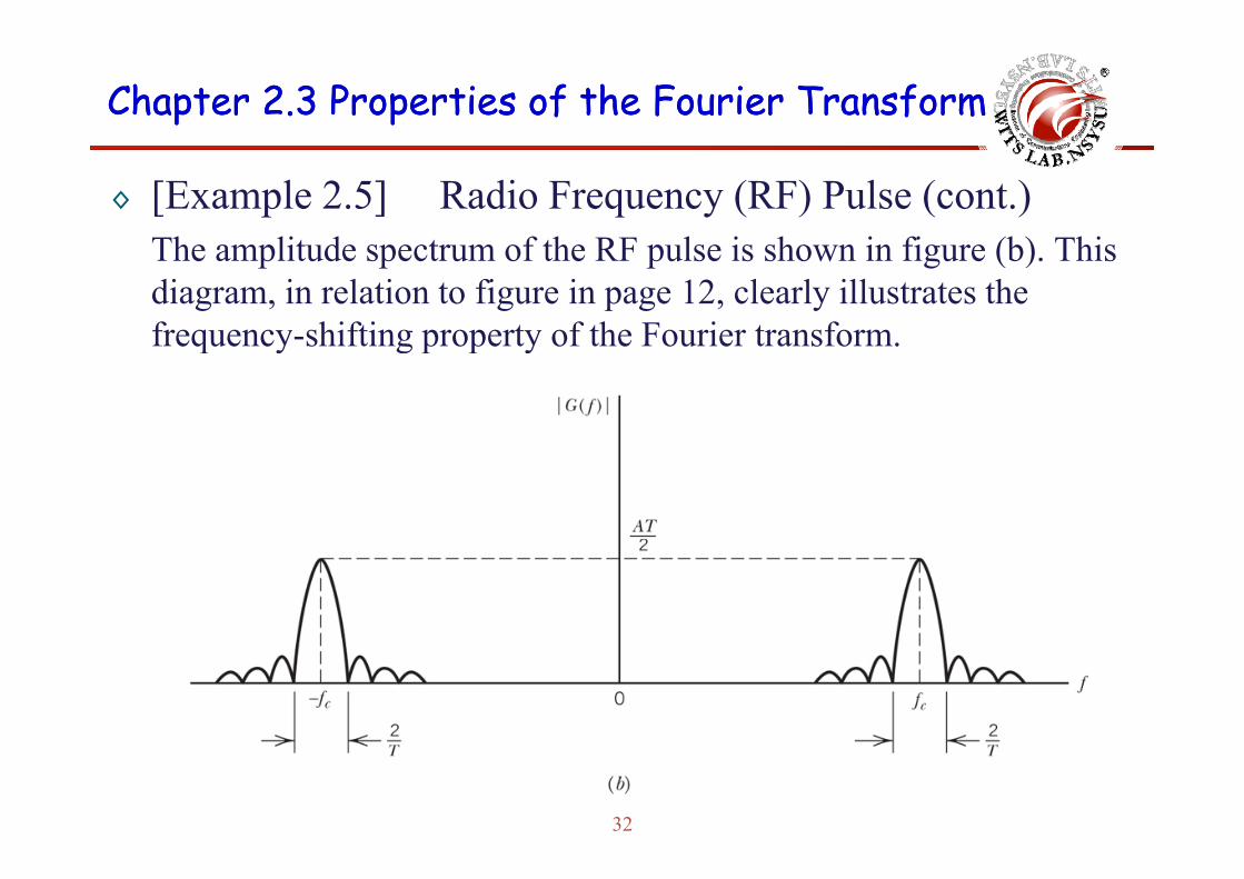
◊ [Example 2.5] Radio Frequency (RF) Pulse (cont.)Th lit d t f th RF l i h i fi (b) ThiThe amplitude spectrum of the RF pulse is shown in figure (b). This diagram, in relation to figure in page 12, clearly illustrates the frequency-shifting property of the Fourier transformfrequency shifting property of the Fourier transform.

32


◊ Property 6：Area Under g(t)∞

∫If , thenThat is, the area under a function g(t) is equal to the value of its

( ) ( ) g t G f ( ) ( )0g t dt G∞

−∞=∫ Physical meaning for G(0)?

Fourier-transform G( f ) at f =0. This result can be obtained by putting f =0 in the formula of Fourier transform.

( ) ( ) ( )∞

∫◊ Property 7：Area Under G( f )

( ) ( ) ( )exp 2G f g t j ft dtπ−∞

= −∫

If , thenThat is the value of a function g(t) at t =0 is equal to the area

( ) ( ) g t G f ( ) ( )0g G f df∞

−∞= ∫

That is, the value of a function g(t) at t 0 is equal to the area under its Fourier-transform G( f ). This result can be obtained by putting t =0 in the formula of inverse Fourier transform.

33

( ) ( ) ( )exp 2g t G f j ft dfπ∞

−∞= ∫


◊ Property 8：Differentiation in the Time DomainL t d th t th fi t d i ti f ( ) i( ) ( )t G fLet , and assume that the first derivative of g(t) is Fourier transformable. Then

( ) ( )g t G f

d

Th t i diff ti ti f ti f ti (t) h th ff t f

( ) ( )2 d g t j f G fdt

π (2.31)

That is, differentiation of a time function g(t) has the effect of multiplying its Fourier transform G( f ) by the factor j2πf. If we assume that the Fourier transform of the higher-order derivativeassume that the Fourier transform of the higher order derivative exists, then

( ) ( ) ( )2n

nn

d g t j f G fdt

π

◊ Proof：This result is obtained by taking the first derivative of both sides of the integral defining the inverse Fourier transform.

dt

34

g g( ) ( ) ( )exp 2g t G f j ft dfπ

∞

−∞= ∫


◊ [Example 2.6] Gaussian PulseW ill d i th ti l f f l i l th t h th◊ We will derive the particular form of a pulse signal that has the same mathematical form as its own Fourier transform.By differentiating the formula for the Fourier transform G( f )◊ By differentiating the formula for the Fourier transform G( f ) with respect to f, we have

( ) ( )2 dj tg t G fdf

π−( ) ( ) ( )exp 2G f g t j ft dtπ∞

= −∫

◊ Add (2.31) plus j times

df

( ) ( )2 d g t j f G fdt

π ( ) ( )2 dj tg t G fdf

π−

( ) ( ) ( )pf g j f−∞∫

f( ) ( ) ( ) ( )2 2

dg t dG ftg t j fG f

dt dfπ π

⎡ ⎤+ +⎢ ⎥

⎣ ⎦

◊ If , then

⎣ ⎦

( ) ( )2dg t

tg tdt

π= − ( ) ( )2dG f

fG fdf

π= −

35

dt df


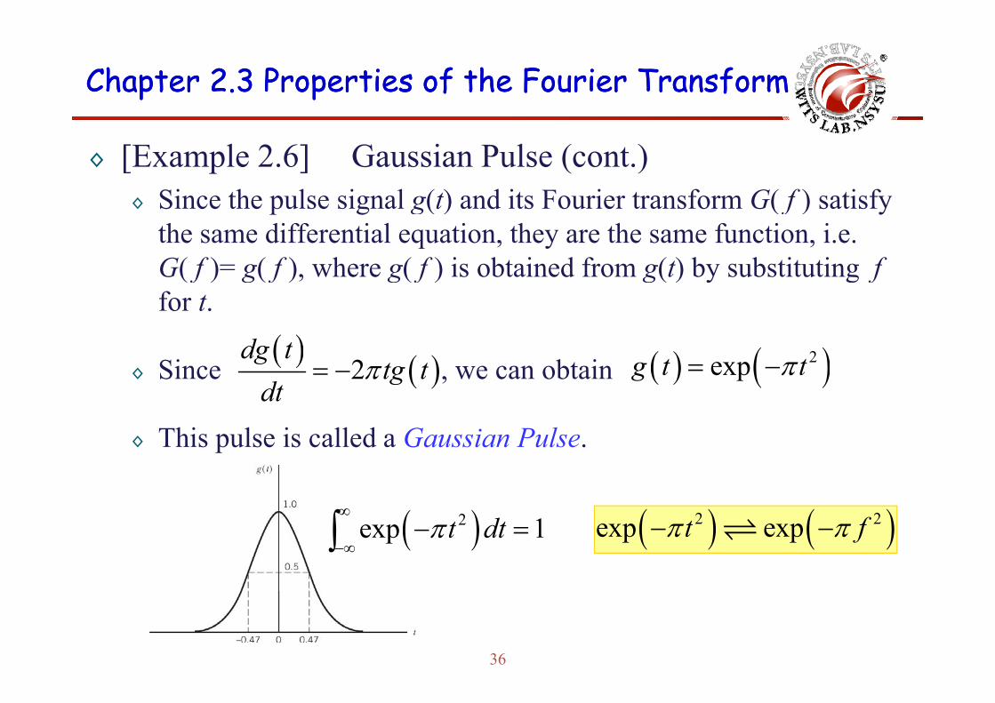
◊ [Example 2.6] Gaussian Pulse (cont.)Si th l i l ( ) d it F i t f G( f ) ti f◊ Since the pulse signal g(t) and its Fourier transform G( f ) satisfy the same differential equation, they are the same function, i.e. G( f )= g( f ) where g( f ) is obtained from g(t) by substituting fG( f ) g( f ), where g( f ) is obtained from g(t) by substituting f for t.

( )dg t ( ) ( )2◊ Since , we can obtain

Thi l i ll d G i P l

( ) ( )2dg t

tg tdt

π= − ( ) ( )2expg t tπ= −

◊ This pulse is called a Gaussian Pulse.

( )∞

∫ ( ) ( )( )2exp 1t dtπ∞

−∞− =∫ ( ) ( )2 2exp expt fπ π− −

36


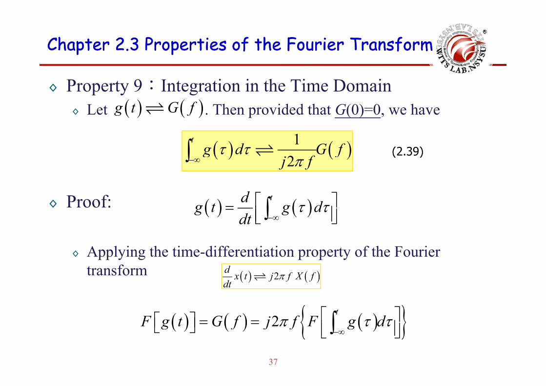
◊ Property 9：Integration in the Time DomainL t Th id d th t G(0) 0 h( ) ( )t G f◊ Let . Then provided that G(0)=0, we have( ) ( )g t G f

( ) ( )1tg d G fτ τ∫ (2 39)( ) ( )

2g d G f

j fτ τ

π−∞∫

d ⎡ ⎤

(2.39)

◊ Proof: ( ) ( )tdg t g d

dtτ τ

−∞

⎡ ⎤= ⎢ ⎥⎣ ⎦∫

◊ Applying the time-differentiation property of the Fourier transform ( ) ( )2 d x t j f X f

dπ

( ) ( ) ( ){ }2t

F g t G f j f F g dπ τ τ⎡ ⎤⎡ ⎤ = =⎣ ⎦ ⎢ ⎥⎣ ⎦∫

( ) ( )j f fdt

37

( ) ( ) ( ){ }2F g t G f j f F g dπ τ τ−∞

⎡ ⎤⎣ ⎦ ⎢ ⎥⎣ ⎦∫


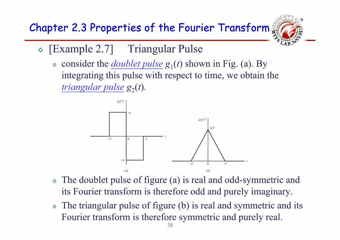
◊ [Example 2.7] Triangular Pulse◊ consider the doublet pulse g1(t) shown in Fig (a) By◊ consider the doublet pulse g1(t) shown in Fig. (a). By

integrating this pulse with respect to time, we obtain the triangular pulse g2(t).

◊ The doublet pulse of figure (a) is real and odd-symmetric and its Fourier transform is therefore odd and purely imaginary.

h i l l f fi (b) i l d i d i

38

◊ The triangular pulse of figure (b) is real and symmetric and its Fourier transform is therefore symmetric and purely real.


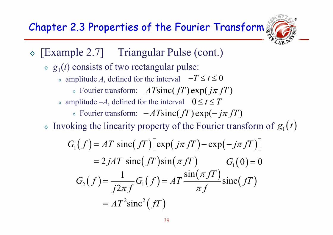
◊ [Example 2.7] Triangular Pulse (cont.)( ) i t f t t l l◊ g1(t) consists of two rectangular pulse: ◊ amplitude A, defined for the interval

◊ Fourier transform:0T t− ≤ ≤

sinc( )exp( )AT fT j fTπ◊ Fourier transform:◊ amplitude –A, defined for the interval

◊ Fourier transform:0 t T≤ ≤

sinc( )exp( )AT fT j fTπ

sinc( )exp( )AT fT j fTπ− −◊ Invoking the linearity property of the Fourier transform of

( ) p( )f j f( )1g t

( ) ( ) ( ) ( )sinc exp expG f AT fT j fT j fTπ π⎡ ⎤= ⎣ ⎦

( )i fT

( ) ( ) ( ) ( )( ) ( )

1 sinc exp exp

2 sinc sin

G f AT fT j fT j fT

jAT fT fT

π π

π

⎡ ⎤= − −⎣ ⎦= ( )1 0 0G =

( ) ( ) ( ) ( )2 1

sin1 sinc2

fTG f G f AT fT

j f fπ

π π= =

39

( )2 2sincAT fT=


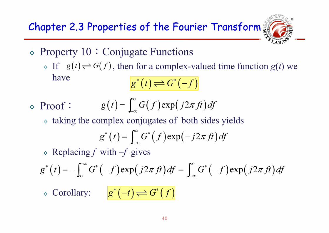
◊ Property 10：Conjugate FunctionsIf th f l l d ti f ti ( )( ) ( )G f◊ If , then for a complex-valued time function g(t) we have

( ) ( )g t G f

( ) ( )g t G f∗ ∗ −

◊ Proof： ( ) ( ) ( )exp 2g t G f j ft dfπ∞

−∞= ∫

◊ taking the complex conjugates of both sides yields

( ) ( ) ( )exp 2g t G f j ft dfπ∞∗ ∗

−∞= −∫

◊ Replacing f with –f gives−∞∫

( ) ( ) ( ) ( ) ( )exp 2 exp 2g t G f j ft df G f j ft dfπ π−∞ ∞∗ ∗ ∗= =∫ ∫

◊ Corollary:

( ) ( ) ( ) ( ) ( )exp 2 exp 2g t G f j ft df G f j ft dfπ π∞ −∞

= − − = −∫ ∫( ) ( )g t G f∗ ∗−

40

y ( ) ( )g f


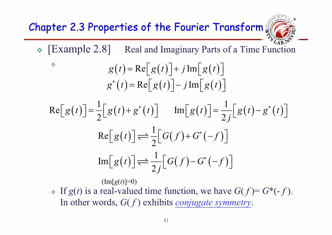
◊ [Example 2.8] Real and Imaginary Parts of a Time Function◊ ( ) ( ) ( )⎡ ⎤ ⎡ ⎤◊ ( ) ( ) ( )Re Img t g t j g t⎡ ⎤ ⎡ ⎤= +⎣ ⎦ ⎣ ⎦

( ) ( ) ( )Re Img t g t j g t∗ ⎡ ⎤ ⎡ ⎤= −⎣ ⎦ ⎣ ⎦( ) ( ) ( )⎣ ⎦ ⎣ ⎦

( ) ( ) ( )1Re2

g t g t g t∗⎡ ⎤⎡ ⎤ = +⎣ ⎦ ⎣ ⎦ ( ) ( ) ( )1Im2

g t g t g tj

∗⎡ ⎤⎡ ⎤ = −⎣ ⎦ ⎣ ⎦2 ⎣ ⎦ 2 j ⎣ ⎦

( ) ( ) ( )1Re2

g t G f G f∗⎡ ⎤⎡ ⎤ + −⎣ ⎦ ⎣ ⎦

( ) ( ) ( )21Im2

g t G f G fj

∗⎡ ⎤⎡ ⎤ − −⎣ ⎦ ⎣ ⎦

◊ If g(t) is a real-valued time function, we have G( f )= G*(- f ).

2 j(Im[g(t)]=0)

41

In other words, G( f ) exhibits conjugate symmetry.


◊ Property 11：Multiplication in the Time DomainL t d Th( ) ( )t G f ( ) ( )t G f◊ Let and .Then( ) ( )1 1g t G f ( ) ( )2 2g t G f

( ) ( ) ( ) ( )1 2 1 2g t g t G G f dλ λ λ∞

−∞−∫

◊ Proof：Let’s denote

−∞∫( ) ( ) ( )1 2 12g t g t G f

◊ For g (t) we have:

( ) ( ) ( ) ( )12 1 2 exp 2G f g t g t j ft dtπ∞

−∞= −∫

( ) ( ) ( )' ' 'exp 2g t G f j f t dfπ∞

∫◊ For g2(t), we have: ( ) ( ) ( )2 2 exp 2g t G f j f t dfπ−∞

= ∫( ) ( ) ( ) ( )' ' '

12 1 2 exp 2G f g t G f j f f t df dtπ∞ ∞

∞ ∞⎡ ⎤= − −⎣ ⎦∫ ∫

◊ Define:

( ) ( )−∞ −∞ ⎣ ⎦∫ ∫

'f fλ = −

⎡ ⎤

42

( ) ( ) ( ) ( )12 2 1 exp 2G f G f g t j t dt dλ πλ λ∞ ∞

−∞ −∞

⎡ ⎤= − −⎢ ⎥⎣ ⎦∫ ∫


◊ The inner integral is recognized as G1(λ)

( ) ( ) ( )∞

∫◊ This integral is known as the convolution integral expressed in

h f d i d h f i ( f ) i f d

( ) ( ) ( )12 1 2G f G G f dλ λ λ∞

−∞= −∫ Q.E.D.

the frequency domain, and the function G12( f ) is referred to as the convolution of G1( f ) and G2( f ).Th lti li ti f t i l i th ti d i i◊ The multiplication of two signals in the time domain is transformed into the convolution of their individual Fourier transforms in the frequency domain This property is known astransforms in the frequency domain. This property is known as the multiplication theorem.

◊ Notation: ( ) ( ) ( )G f G f G f∗( ) ( ) ( )12 1 2G f G f G f= ∗

( ) ( ) ( ) ( )1 2 1 2g t g t G f G f∗

43

( ) ( ) ( ) ( )1 2 2 1G f G f G f G f∗ = ∗


◊ Property 12：Convolution in the Time DomainL t d th( ) ( )t G f ( ) ( )t G f◊ Let and , then( ) ( )1 1g t G f ( ) ( )2 2g t G f

( ) ( ) ( ) ( )1 2 1 2g g t d G f G fτ τ τ∞

−∫◊ Proof：

( ) ( ) ( ) ( )1 2 1 2g g f f−∞∫

2( ) ( ) ( ) j ftg t G f G f e dfπ∞= ∫12 1 2

2 21 2

( ) ( ) ( )

= ( ) ( )

j f

j uf j ft

g t G f G f e df

G f g u e du e dfπ π

−∞

∞ ∞ −

=

⎡ ⎤⎢ ⎥⎣ ⎦

∫

∫ ∫1 2( ) ( )

Let

f g f

t uλ−∞ −∞⎢ ⎥⎣ ⎦

= −

⎡ ⎤

∫ ∫

( )

( ) ( )

22 1 = ( ) j fg t G f e df dπ λλ λ

∞ ∞

−∞ −∞

∞

⎡ ⎤−⎢ ⎥⎣ ⎦∫ ∫

∫44

( ) ( )1 2 = g g t dλ λ λ−∞

−∫ Q.E.D.


◊ We may thus state that the convolution of two signals in the time domain is transformed into the multiplication of their individualdomain is transformed into the multiplication of their individual Fourier transforms in the frequency domain.

◊ This property is known as the convolution theorem.p p y

◊ Property 11 and property 12 are the dual of each other.◊ Property 11 and property 12 are the dual of each other.

◊ Shorthand notation for convolution:◊ Shorthand notation for convolution:

( ) ( ) ( ) ( )1 2 1 2g t g t G f G f∗

45


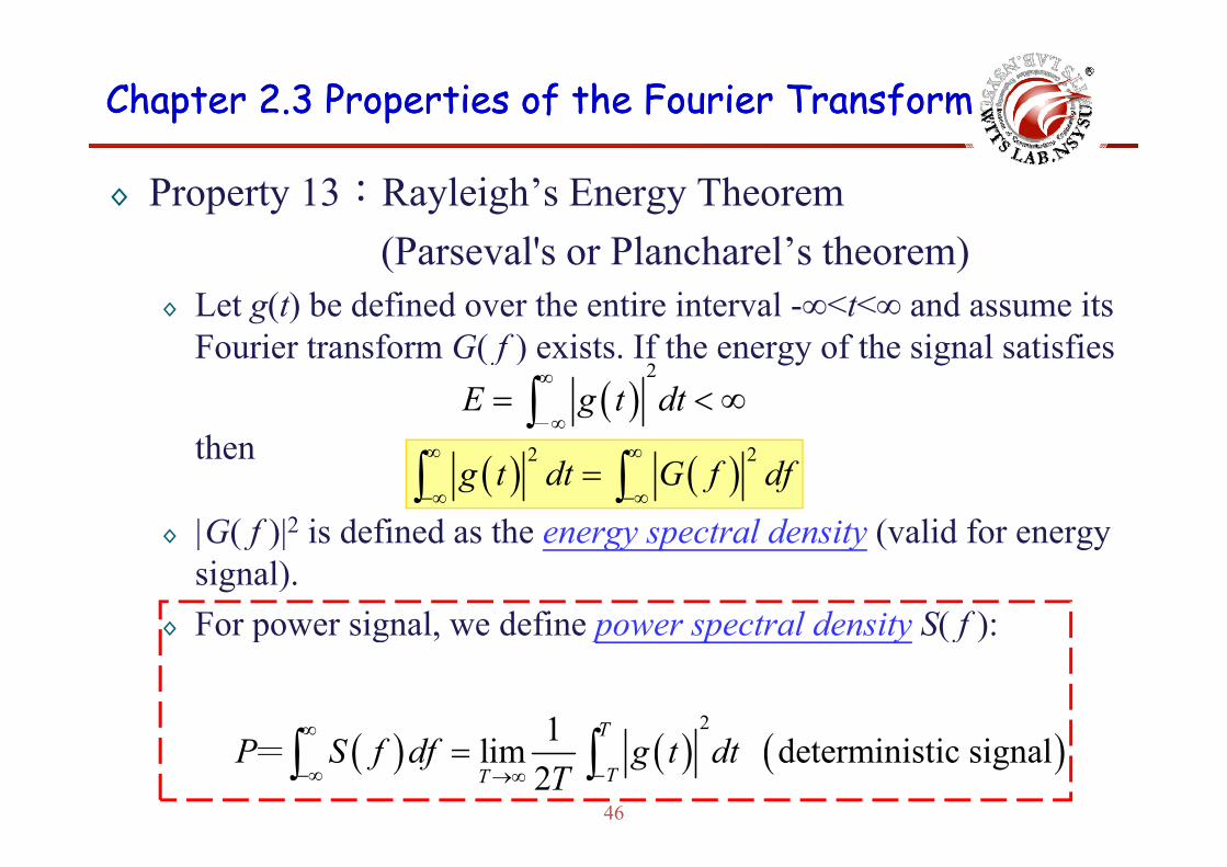
◊ Property 13：Rayleigh’s Energy Theorem( l' l h l’ h )(Parseval's or Plancharel’s theorem)

◊ Let g(t) be defined over the entire interval -∞<t<∞ and assume its F i f G( f ) i If h f h i l i fiFourier transform G( f ) exists. If the energy of the signal satisfies

( )2

E g t dt∞

∞= < ∞∫－

then

◊ |G( f )|2 is defined as the energy spectral density (valid for energy( ) ( )2 2

g t dt G f df∞ ∞

−∞ −∞=∫ ∫

◊ |G( f )|2 is defined as the energy spectral density (valid for energy signal).

◊ For power signal we define power spectral density S( f ):◊ For power signal, we define power spectral density S( f ):

21 T∞

∫ ∫46

( ) ( ) ( )21lim deterministic signal

2T

TTP S f df g t dt

T∞

−∞ −→∞=∫ ∫＝


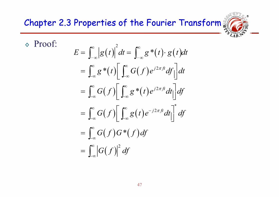
◊ Proof:( ) ( ) ( )

2

*E g t dt g t g t dt∞ ∞

= = ⋅∫ ∫( ) ( ) ( )

( ) ( ) 2* j ft

E g t dt g t g t dt

g t G f e df dtπ

∞ ∞

∞ ∞

∞ ∞

⎡ ⎤= ⎢ ⎥⎣ ⎦

∫ ∫

∫ ∫－－

( ) ( ) 2* j ftG f g t e dt dfπ

−∞ −∞

∞ ∞

−∞ −∞

⎢ ⎥⎣ ⎦⎡ ⎤= ⎢ ⎥⎣ ⎦

∫ ∫

∫ ∫

( ) ( )*

2j ftG f g t e dt dfπ∞ ∞ −

−∞ −∞

⎣ ⎦

⎡ ⎤= ⎢ ⎥⎣ ⎦∫ ∫( ) ( )*G f G f df

∞

−∞

⎣ ⎦

= ∫( ) 2

G f df∞

−∞= ∫

47


◊ [Example 2.9] Sinc Pulse (continued)C id th i l A i (2W ) Th f thi l◊ Consider the sinc pulse A sinc(2Wt). The energy of this pulse equals

( )2 2sinc 2E A Wt dt∞

= ∫◊ The integral in the right-hand side of this equation is rather

difficult to evaluate

( )−∞∫

difficult to evaluate.◊ From example 2.4, the Fourier transform of the sinc pulse A

sinc(2Wt) is equal to (A/2W)rect( f /2W). Applying Rayleigh’ssinc(2Wt) is equal to (A/2W)rect( f /2W). Applying Rayleigh s energy theorem 2

2rectA fE df∞⎛ ⎞ ⎛ ⎞= ⎜ ⎟ ⎜ ⎟∫

2 2

rect2 2

W

E dfW W

A Adf

−∞⎜ ⎟ ⎜ ⎟⎝ ⎠ ⎝ ⎠

⎛ ⎞⎜ ⎟

∫

∫48

2 2Wdf

W W−= =⎜ ⎟⎝ ⎠ ∫


◊ Summary of Properties for Fourier Transform

g(t) RealValued

Symmetric Asymmetric Real Valued and Symmetric

Real Valued andOdd Symmetric

G( f )Spectrum

Conjugate Symmetry

Real Valued

Complex Valued

Real Valued and Symmetric

Odd and PurelyImaginary

◊ Compression of a function in the time domain is equivalent to the expansion of its Fourier transform in the frequency domain, or viceexpansion of its Fourier transform in the frequency domain, or vice versa.

49

Chapter 2.4Chapter 2.4The Inverse Relationship The Inverse Relationship The Inverse Relationship The Inverse Relationship

between Time and Frequencybetween Time and Frequency


Chapter 2.4 The Inverse Relationship between Chapter 2.4 The Inverse Relationship between Time and FrequencyTime and FrequencyTime and FrequencyTime and Frequency

◊ The time-domain and frequency-domain description of a signal are inversely related:signal are inversely related:◊ If the time-domain description of a signal is changed, then the

frequency domain description of the signal is changed in anfrequency-domain description of the signal is changed in an inverse manner, and vice versa.

◊ If a signal is strictly limited in frequency then the time-domain◊ If a signal is strictly limited in frequency, then the time-domain description of the signal will trail on indefinitely.◊ A signal is strictly limited in frequency or strictly band limited if its g y q y y

Fourier transform is exactly zero outside a finite band of frequencies.

◊ If a signal is strictly limited in time, then the spectrum of the i l i i fi i isignal is infinite in extent.◊ A signal is strictly limited in time if the signal is exactly zero outside a

finite time interval.

51

finite time interval.

Chapter 2.4 The Inverse Relationship between Chapter 2.4 The Inverse Relationship between Time and FrequencyTime and Frequency

◊ Bandwidth

Time and FrequencyTime and Frequency

◊ The bandwidth of a signal provides a measure of the extent of significant spectral content of the signal for positive frequencies.◊ When the signal is strictly band limited, the bandwidth is well defined.

When the signal is not strictly band limited there is no universally◊ When the signal is not strictly band-limited, there is no universally accepted definition of bandwidth.

◊ A signal is said to be low-pass if its significant spectral content is centered around the origin.

◊ A signal is said to be band-pass if its significant spectral content is centered around ±f , where f is a nonzero frequency.

52

content is centered around ±fc, where fc is a nonzero frequency.


◊ Bandwidth (cont.)Wh th t f i l i t i ith i l b


◊ When the spectrum of a signal is symmetric with a main lobe bounded by well-defined nulls(i.e. frequencies at which the spectrum is zero) we may use the main lobe as the basis forspectrum is zero), we may use the main lobe as the basis for defining the bandwidth of the signal.

◊ When the signal is low-pass, the bandwidth is defined as one half the total width of the main spectral lobe, since only one h lf f thi l b li i id th iti f ihalf of this lobe lies inside the positive frequency region.

◊ When the signal is band-pass with main spectral lobes centered◊ When the signal is band pass with main spectral lobes centered around ±fc, where fc is large, the bandwidth is defined as the width of the main lobe for positive frequency. This definition

53

of bandwidth is called the null-to-null bandwidth.


◊ Bandwidth (cont.)


54


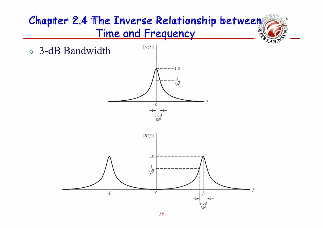
◊ 3-dB Bandwidth


◊ When the signal is low-pass, the 3-dB bandwidth is defined as the separation between zero frequency, where the amplitude spectrum attains its peak value and the positive frequency atspectrum attains its peak value, and the positive frequency at which the amplitude spectrum drops to of its peak value.

◊ When the signal is band-pass centered at ±f the 3-dB1/ 2

◊ When the signal is band-pass, centered at ±fc, the 3-dB bandwidth is defined as the separation (along the positive frequency axis) between the two frequencies at which the q y ) qamplitude spectrum of the signal drops to of the peak value at fc.

1/ 2

◊ Advantage : it can be read directly from a plot of the amplitude spectrum.

i d i b i l di if h li d

55

◊ Disadvantage: it may be misleading if the amplitude spectrum has slowly decreasing tails.

Ch a p t e r 2 .4 T h e I nve r s e Re la t ions h ip b e t we e n Chapter 2.4 The Inverse Relationship between Time and FrequencyTime and Frequency

◊ 3-dB BandwidthTime and FrequencyTime and Frequency

56


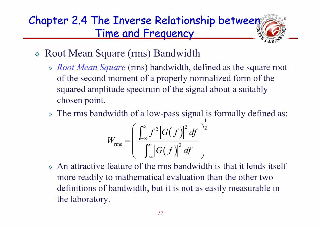
◊ Root Mean Square (rms) Bandwidth


◊ Root Mean Square (rms) bandwidth, defined as the square root of the second moment of a properly normalized form of the

d lit d t f th i l b t it blsquared amplitude spectrum of the signal about a suitably chosen point.

◊ The rms bandwidth of a low pass signal is formally defined as:◊ The rms bandwidth of a low-pass signal is formally defined as:

( )1

2 22f G f dfW

∞

−∞

⎛ ⎞⎜ ⎟∫

An attractive feature of the rms bandwidth is that it lends itself

( )rms 2

WG f df

∞∞

−∞

⎜ ⎟=⎜ ⎟⎝ ⎠

∫∫

◊ An attractive feature of the rms bandwidth is that it lends itself more readily to mathematical evaluation than the other two definitions of bandwidth, but it is not as easily measurable in

57

definitions of bandwidth, but it is not as easily measurable in the laboratory.


◊ Time-Bandwidth product


◊ For any family of pulse signals (e.g. the exponential pulse) that differ in time scale, the product of the signal’s duration

d it b d idth i l t t h band its bandwidth is always a constant, as shown by

Th d t i ll d th ti b d idth d t(duration) (bandwidth) constant⋅ =

◊ The product is called the time-bandwidth product or bandwidth-duration product.

◊ If the duration of a pulse signal is decreased by reducing the time scale by a factor a the frequency scale of the signal’stime scale by a factor a, the frequency scale of the signal s spectrum, and therefore the bandwidth of the signal, is increased by the same factor a.

58


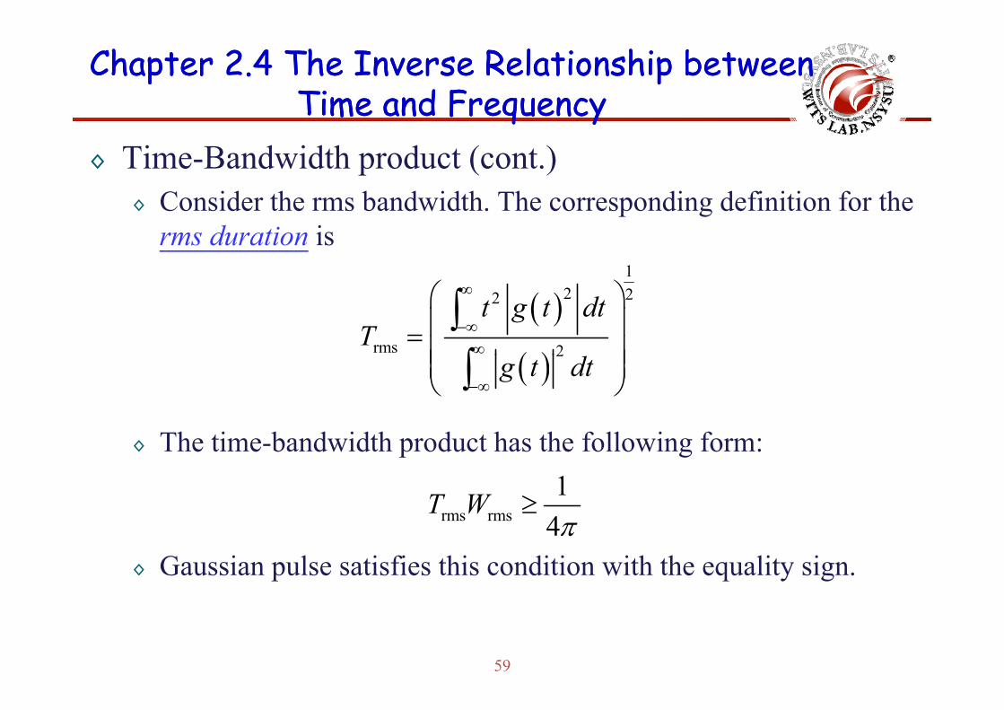
◊ Time-Bandwidth product (cont.)C id th b d idth Th di d fi iti f th


◊ Consider the rms bandwidth. The corresponding definition for the rms duration is

1

( )

( )

12 22

rms 2

t g t dtT

∞

−∞∞

⎛ ⎞⎜ ⎟= ⎜ ⎟⎜ ⎟

∫∫

Th ti b d idth d t h th f ll i f

( ) 2g t dt

−∞

⎜ ⎟⎜ ⎟⎝ ⎠∫

◊ The time-bandwidth product has the following form:

rms rms1

4T W ≥

◊ Gaussian pulse satisfies this condition with the equality sign.

rms rms 4π

59

Chapter 2.5Chapter 2.5Dirac Delta FunctionDirac Delta FunctionDirac Delta FunctionDirac Delta Function


Chapter 2.5 Dirac Delta FunctionChapter 2.5 Dirac Delta Function

◊ The Dirac delta function, denoted by δ(t), is defined as having zero amplitude everywhere except at t = 0 where it is infinitely large inamplitude everywhere except at t 0, where it is infinitely large in such a way that it contains unit area under its curve; i.e.

( ) ( )∞

∫◊ The delta function δ(t) is an even function of time t.

( ) 0, 0t tδ = ≠ ( ) 1t dtδ∞

−∞=∫

◊ The delta function δ(t) is an even function of time t.◊ Sifting property of the delta function:

( ) ( ) ( )0 0g t t t dt g tδ∞

−∞− =∫

◊ Replication property of the delta function: the convolution of any function with the delta function leaves that function unchanged.

61

( ) ( ) ( ) ( ) ( )g t t g t d g tδ τ δ τ τ∞

−∞∗ = − =∫


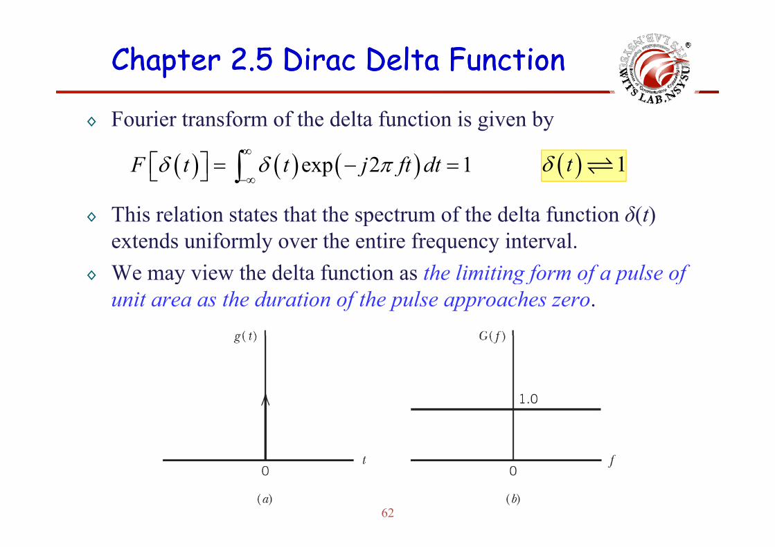
◊ Fourier transform of the delta function is given by∞

This relation states that the spectr m of the delta f nction δ(t)

( ) ( ) ( )exp 2 1F t t j ft dtδ δ π∞

−∞⎡ ⎤ = − =⎣ ⎦ ∫ ( ) 1tδ

◊ This relation states that the spectrum of the delta function δ(t) extends uniformly over the entire frequency interval.

◊ We may view the delta function as the limiting form of a pulse of◊ We may view the delta function as the limiting form of a pulse of unit area as the duration of the pulse approaches zero.

62

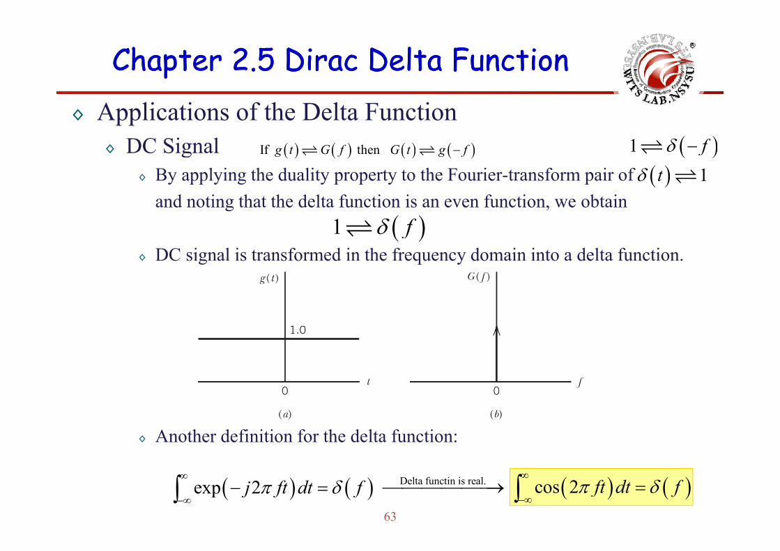
Chapter 2.5 Dirac Delta FunctionChapter 2.5 Dirac Delta Function◊ Applications of the Delta Function

◊ DC Signal ( ) ( ) ( ) ( )If theng t G f G t g f− ( )1 fδ −◊ DC Signal◊ By applying the duality property to the Fourier-transform pair of

and noting that the delta function is an even function, we obtain( ) 1tδ

( ) ( ) ( ) ( )If then g t G f G t g f− ( )1 fδ

◊ DC signal is transformed in the frequency domain into a delta function.( )1 fδ

◊ Another definition for the delta function:

63

( ) ( )exp 2j ft dt fπ δ∞

−∞− =∫ ( ) ( )cos 2 ft dt fπ δ

∞

−∞=∫Delta functin is real.⎯⎯⎯⎯⎯⎯→


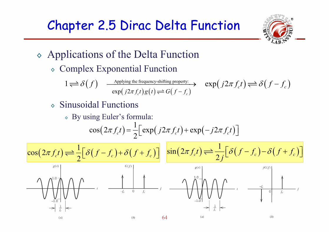
◊ Applications of the Delta Function◊ Complex Exponential Function

( ) ( )exp 2 c cj f t f fπ δ −( )1 fδ( ) ( ) ( )2j f G f f

Applying the frequency-shifting property:⎯⎯⎯⎯⎯⎯⎯⎯⎯⎯→

◊ Sinusoidal FunctionsBy using Euler’s formula:

( ) ( ) ( )exp 2 c cj f t g t G f fπ −

◊ By using Euler s formula:

( ) ( ) ( )1cos 2 exp 2 exp 22c c cf t j f t j f tπ π π⎡ ⎤= + −⎣ ⎦

( ) ( ) ( )1cos 22c c cf t f f f fπ δ δ⎡ ⎤− + +⎣ ⎦ ( ) ( ) ( )1sin 2

2c c cf t f f f fj

π δ δ⎡ ⎤− − +⎣ ⎦

64


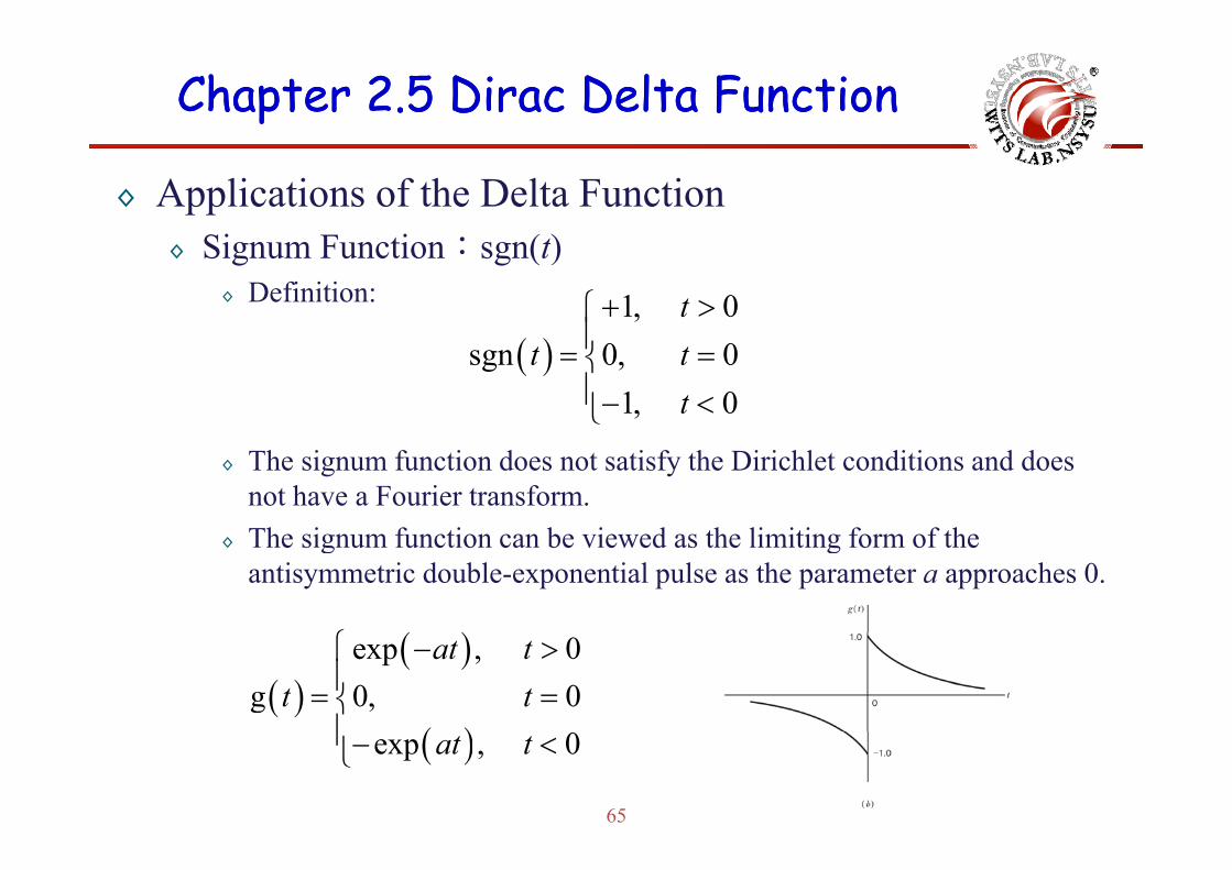
◊ Applications of the Delta FunctionSi F ti ： ( )◊ Signum Function：sgn(t)◊ Definition: 1, 0t+ >⎧

⎪( )sgn 0, 01, 0

t tt

⎪= =⎨⎪− <⎩

◊ The signum function does not satisfy the Dirichlet conditions and does not have a Fourier transform.Th i f ti b i d th li iti f f th◊ The signum function can be viewed as the limiting form of the antisymmetric double-exponential pulse as the parameter a approaches 0.

( )⎧

( )( )

( )

exp , 0g 0, 0

at tt t

⎧ − >⎪= =⎨⎪

65

( )exp , 0at t⎪− <⎩


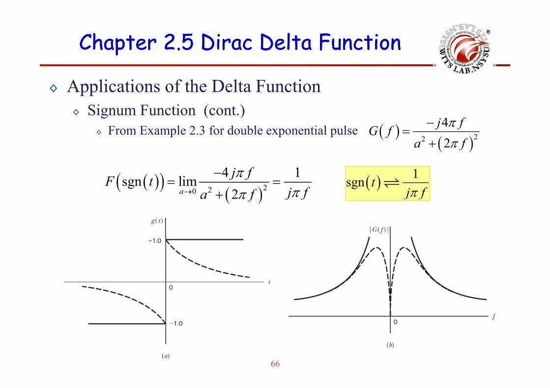
◊ Applications of the Delta FunctionSi F ti ( t )◊ Signum Function (cont.)◊ From Example 2.3 for double exponential pulse ( )

( )22

42

j fG fa f

ππ

−=

+ ( )f

( )( )( )220

4 1sgn lim2a

j fF tj fa f

πππ→

−= =

+( ) 1sgn t

j fπ( )2 j fa f ππ+ j fπ

66


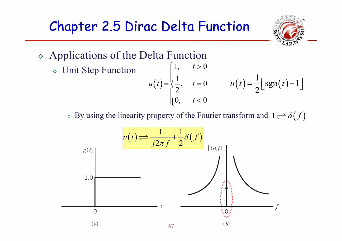
◊ Applications of the Delta Function1 0t >⎧◊ Unit Step Function

( )

1, 01 , 02

t

u t t

>⎧⎪⎪= =⎨⎪

( ) ( )1 sgn 12

u t t⎡ ⎤= +⎣ ⎦

◊ By using the linearity property of the Fourier transform and

0, 0t⎪

<⎪⎩

( )1 fδ

( ) ( )1 12 2

u t fj f

δπ

+

( )

67


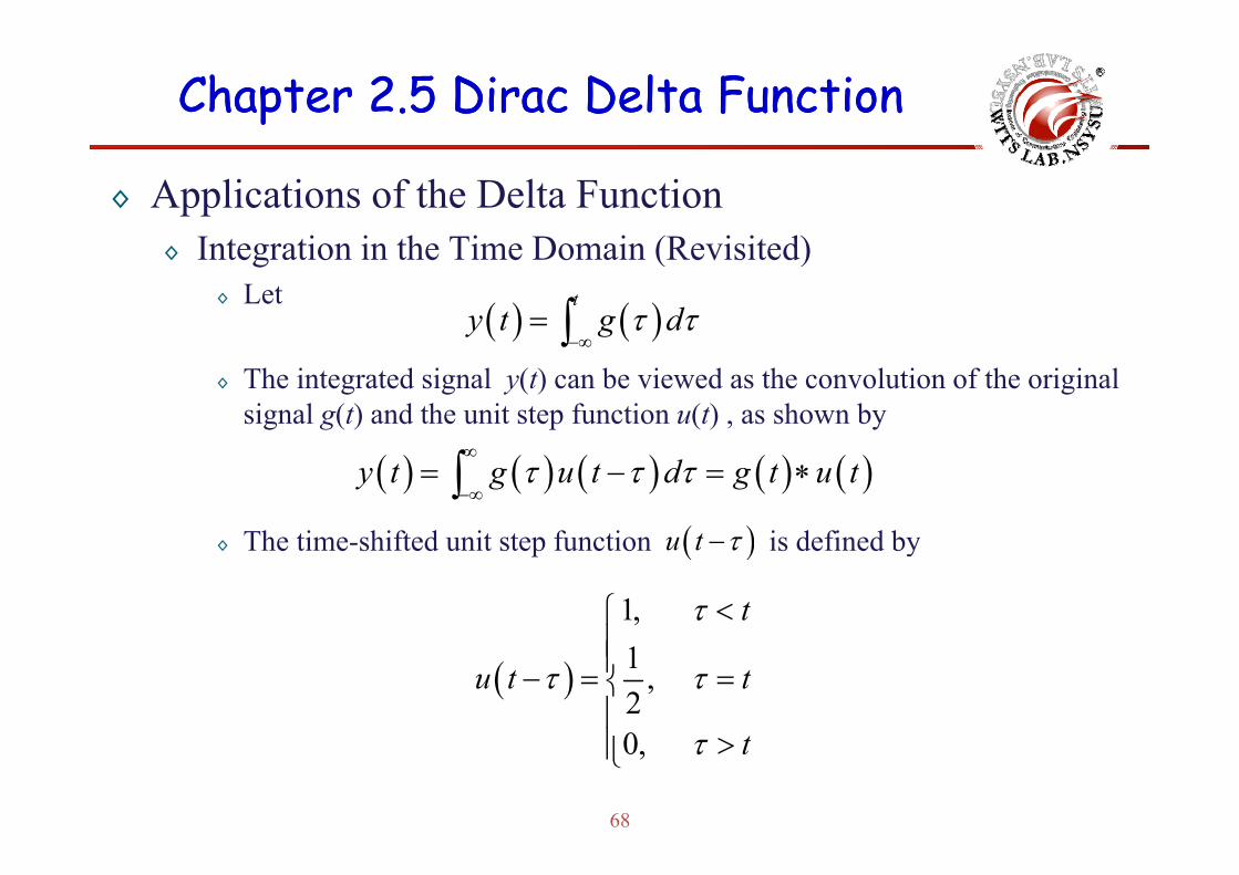
◊ Applications of the Delta FunctionI t ti i th Ti D i (R i it d)◊ Integration in the Time Domain (Revisited)◊ Let

( ) ( )t

y t g dτ τ= ∫◊ The integrated signal y(t) can be viewed as the convolution of the original

signal g(t) and the unit step function u(t) , as shown by

( ) ( )−∞∫

Th ti hift d it t f ti i d fi d b

( ) ( ) ( ) ( ) ( )y t g u t d g t u tτ τ τ∞

−∞= − = ∗∫

( )t τ◊ The time-shifted unit step function is defined by( )u t τ−

1, tτ <⎧⎪

( ) 1 , 20

u t tτ τ⎪⎪− = =⎨⎪⎪⎩

68

0, tτ >⎪⎩


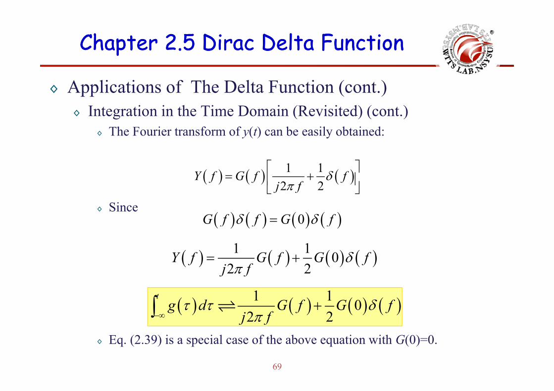
◊ Applications of The Delta Function (cont.)I t ti i th Ti D i (R i it d) ( t )◊ Integration in the Time Domain (Revisited) (cont.)◊ The Fourier transform of y(t) can be easily obtained:

( ) ( ) ( )1 12 2

Y f G f fj f

δπ

⎡ ⎤= +⎢ ⎥

⎣ ⎦◊ Since

( ) ( ) ( ) ( )0G f f G fδ δ=

( ) ( ) ( ) ( )1 1 02 2

Y f G f G fj f

δπ

= +

( ) ( ) ( ) ( )1 1 02 2

tg d G f G f

j fτ τ δ

π−∞+∫

69

◊ Eq. (2.39) is a special case of the above equation with G(0)=0.

Chapter 2.6Chapter 2.6Fourier Transform of Periodic SignalsFourier Transform of Periodic SignalsFourier Transform of Periodic SignalsFourier Transform of Periodic Signals


Chapter 2.6 Fourier Transform of Periodic SignalsChapter 2.6 Fourier Transform of Periodic Signals

◊ A periodic signal can be represented in terms of a Fourier transform provided that this transform is permitted to include delta functionsprovided that this transform is permitted to include delta functions.

◊ Consider a periodic signal g (t) of period T :◊ Consider a periodic signal gT0(t) of period T0:

( ) ( )0exp 2T ng t c j nf tπ∞

= ∑

where cn is the complex Fourier coefficient defined by

( ) ( )0 0pT n

n

g j f=−∞∑

( ) ( )0

0

2

02

1 exp 2T

n TTc g t j nf t dt

Tπ= −∫

and f0 is the fundamental frequency f0=1/T0.

( ) ( )0

0 20

TT −∫

71

Chapter 2.6 Fourier Transform of Periodic SignalsChapter 2.6 Fourier Transform of Periodic Signals◊ Let g(t) be a pulse like function, which equals gT0(t) over one

period and is zero elsewhere; that is,

( ) ( )0

0 0, 2 2TT Tg t t

g t⎧ − ≤ ≤⎪= ⎨⎪

◊ gT0(t) may now be expressed in terms of the function g(t)

( )0, elsewhere⎪⎩

gT0( ) y p g( )

( ) ( )0 0T

m

g t g t mT∞

= ∞

= −∑◊ g(t) is Fourier transformable and can be viewed as a generating

function, which generates the periodic signal gT0(t).

m=−∞

0

( ) ( ) ( ) ( ) ( )0

00

2

0 0 0 0 020

1 exp 2 exp 2T

n TTc g t j nf t dt f g t j nf t dt f G nf

Tπ π

∞

− −∞= − = − ≡∫ ∫

72

where G(nf0) is the Fourier transform of g(t) at the frequency nf0.


◊ The formula for the reconstruction of the periodic signal gT0(t) can be rewritten as: ( )0 0c f G nf=

( ) ( ) ( ) ( )0 0 0 0 0exp 2 exp 2T n

n n

g t c j nf t f G nf j nf tπ π∞ ∞

=−∞ =−∞

= =∑ ∑( )0 0nc f G nf

n n= ∞ = ∞

( ) ( ) ( ) ( )0 0 0 0 0exp 2Tg t g t mT f G nf j nf tπ

∞ ∞

= − =∑ ∑The above equation is one form of Poisson’s sum formula.

m n=−∞ =−∞

( ) ( )exp 2 c cj f t f fπ δ −

( ) ( ) ( )0 0 0 0m n

g t mT f G nf f nfδ∞ ∞

=−∞ =−∞

− −∑ ∑ (2.88)

◊ The Fourier transform of a periodic signal consists of delta functions occurring at integer multiples of the fundamental f f 1/T i l di h i i d h h d l f i

73

frequency f0=1/T0, including the origin, and that each delta function is weighted by a factor equal to the corresponding value of G(nf0).


◊ The function g(t), constituting one period of the periodic signal g (t) has a continuous spectrum defined by G( f )signal gT0(t), has a continuous spectrum defined by G( f ).

◊ The periodic signal gT0(t) has a discrete spectrum.

◊ Periodicity in the time domain has the effect of changing the frequency-domain description or spectrum of thethe frequency domain description or spectrum of the signal into a discrete form defined at integer multiples of the fundamental frequencythe fundamental frequency.

74


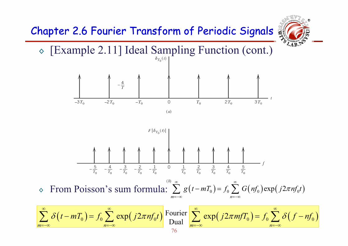
◊ [Example 2.11] Ideal Sampling Function◊ An ideal sampling function or Dirac comb consists of an infinite◊ An ideal sampling function, or Dirac comb, consists of an infinite

sequence of uniformly spaced delta functions.

( ) ( )t t mTδ δ∞

= ∑◊ The generating function g(t) for the ideal sampling function δT0(t)

( ) ( )0 0T

m

t t mTδ δ=−∞

= −∑

consists of the delta function δ(t). We therefore have G( f )=1 and G(nf0)=1 for all n.U i E (2 88) i ld( ) ( ) ( )g t mT f G nf f nfδ

∞ ∞

∑ ∑◊ Using Eq. (2.88) yields( ) ( ) ( )0 0 0 0m n

g t mT f G nf f nfδ=−∞ =−∞

− −∑ ∑

( ) ( )t mT f f nfδ δ∞ ∞

∑ ∑◊ The Fourier transform of a periodic train of delta functions, spaced T0

( ) ( )0 0 0m n

t mT f f nfδ δ=−∞ =−∞

− −∑ ∑

75

seconds apart, consists of another set of delta functions weighted by the factor f0=1/ T0 and regularly spaced f0 Hz apart along the frequency axis.


◊ [Example 2.11] Ideal Sampling Function (cont.)

◊ From Poisson’s sum formula: ( ) ( ) ( )0 0 0 0exp 2m n

g t mT f G nf j nf tπ∞ ∞

=−∞ =−∞

− =∑ ∑

76

( ) ( )0 0 0exp 2m n

t mT f j nf tδ π∞ ∞

=−∞ =−∞

− =∑ ∑ ( ) ( )0 0 0exp 2m n

j mfT f f nfπ δ∞ ∞

=−∞ =−∞

= −∑ ∑FourierDual

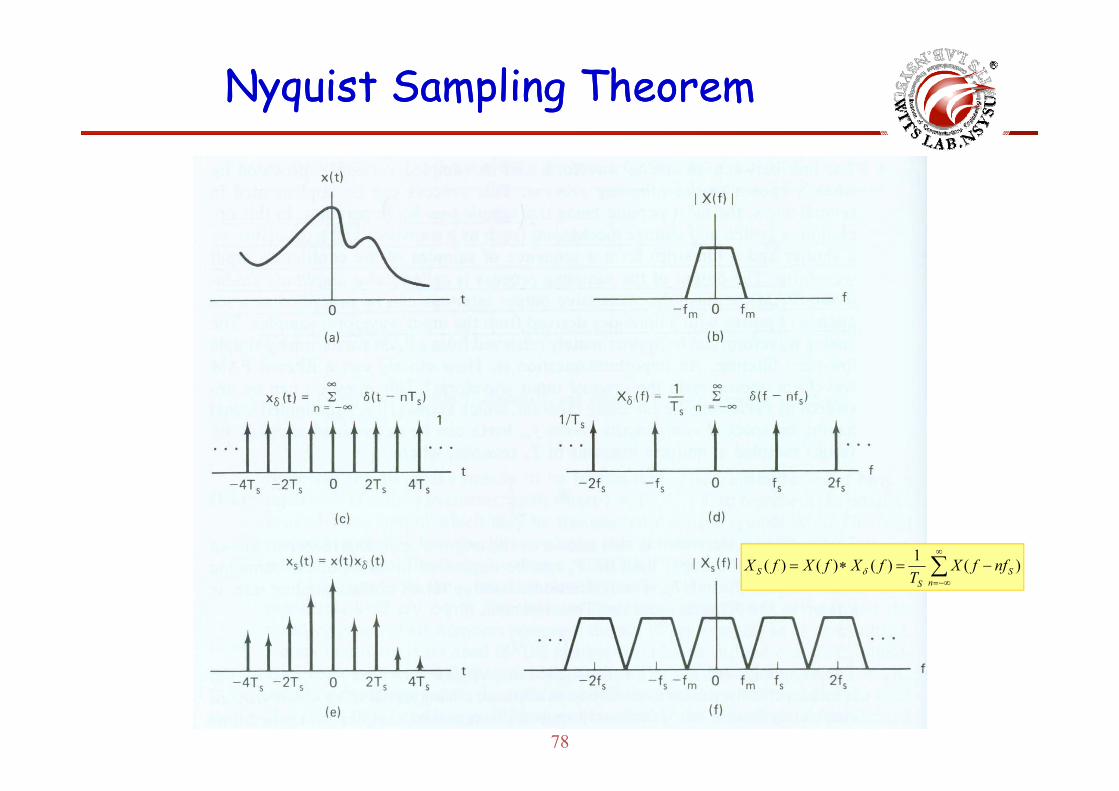
NyquistNyquist Sampling Sampling TheoremTheoremyqyq p gp g

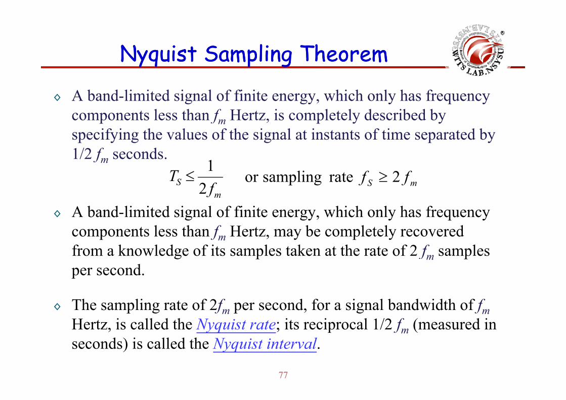
◊ A band-limited signal of finite energy, which only has frequency l h f i l l d ib d bcomponents less than fm Hertz, is completely described by

specifying the values of the signal at instants of time separated by 1/2 f seconds1/2 fm seconds.

mS f

T21

≤ mS ff 2 rate samplingor ≥

◊ A band-limited signal of finite energy, which only has frequency components less than fm Hertz, may be completely recovered f k l d f i l k h f 2 f lfrom a knowledge of its samples taken at the rate of 2 fm samples per second.

◊ The sampling rate of 2fm per second, for a signal bandwidth of fmHertz, is called the Nyquist rate; its reciprocal 1/2 fm (measured in

77

seconds) is called the Nyquist interval.

NyquistNyquist Sampling Sampling TheoremTheorem

∑∞

−=∗= SS nffXT

fXfXfX )(1)()()( δ ∑−∞=nST

78

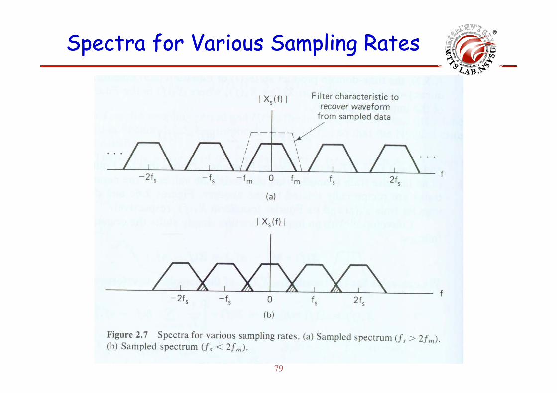
Spectra for Various Sampling RatesSpectra for Various Sampling Rates

79

Chapter 2.7Chapter 2.7ppTransmission of Signals Through Transmission of Signals Through

Linear SystemsLinear SystemsLinear SystemsLinear Systems


Chapter 2.7 Transmission of Signals Through Chapter 2.7 Transmission of Signals Through Linear SystemsLinear SystemsLinear SystemsLinear Systems

◊ System: any physical device that produces an output signal in response to an input signalresponse to an input signal.

◊ Excitation: input signal.◊ Response: output signal◊ Response: output signal.◊ In a linear system, the principle of superposition holds, i.e., the

response of a linear system to a number of excitations appliedresponse of a linear system to a number of excitations applied simultaneously is equal to the sum of the responses of the system when each excitation is applied individually.◊ Important examples: filters, communication channels.

◊ Filter: a frequency-selective device that is used to limit the spectrum f i l b d f f iof a signal to some band of frequencies.

◊ Channel: transmission medium that connects the transmitter and i f i ti t

81

receiver of a communication system.

Chapter 2.7 Transmission of Signals Through Chapter 2.7 Transmission of Signals Through Linear SystemsLinear Systems

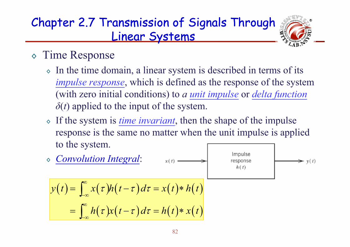
◊ Time ResponseI th ti d i li t i d ib d i t f it

Linear SystemsLinear Systems

◊ In the time domain, a linear system is described in terms of its impulse response, which is defined as the response of the system (with zero initial conditions) to a unit impulse or delta function(with zero initial conditions) to a unit impulse or delta functionδ(t) applied to the input of the system.

◊ If the system is time invariant, then the shape of the impulse ◊ t e syste s time inva iant, t e t e s ape o t e pu seresponse is the same no matter when the unit impulse is applied to the system.

◊ Convolution Integral:

( ) ( ) ( ) ( ) ( )

( ) ( ) ( ) ( )

y t x h t d x t h t

h d h

τ τ τ∞

−∞

∞

= − = ∗∫∫

82

( ) ( ) ( ) ( )h x t d h t x tτ τ τ−∞

= − = ∗∫


◊ Causality and Stability


◊ Causal: A system is said to be causal if it does not respond before the excitation is applied.

F li i i i (LTI) b l h i l◊ For a linear time-invariant (LTI) system to be causal, the impulse response h(t) must vanish for negative time, i.e. h(t)=0, t<0.

◊ A system operating in real time to be physically realizable, it must be y p g p y y ,causal.

◊ The system can be noncausal and yet physically realizable.

bl i id b bl if h i l i◊ Stable: A system is said to be stable if the output signal is bounded for all bounded input signals.

Bounded input bounded output (BIBO) stability criterion◊ Bounded input-bounded output (BIBO) stability criterion.◊ For a LTI system to be stable, the impulse response must be absolutely

integrable, i.e.

83

( )h t dt∞

−∞< ∞∫ (2.100)


◊ Frequency Response◊ Consider a LTI system of impulse response h(t) driven by a


◊ Consider a LTI system of impulse response h(t) driven by a complex exponential input of unit amplitude and frequency f

( ) ( )exp 2x t j ftπ=◊ The response of the system is obtained as

( ) ( )exp 2x t j ftπ

( ) ( ) ( ) ( ) ( )exp 2y t h t x t h j f t dτ π τ τ∞

⎡ ⎤= ∗ = ⎣ ⎦∫( ) ( ) ( ) ( ) ( )

( ) ( ) ( )

exp 2

exp 2 exp 2

y t h t x t h j f t d

j ft h j f d

τ π τ τ

π τ π τ τ

−∞

∞

⎡ ⎤= ∗ = −⎣ ⎦

= −

∫∫

◊ Transfer function of the system is defined as the Fourier transform of its impulse response

( ) ( ) ( )−∞∫

p p

( ) ( ) ( )exp 2H f h t j ft dtπ∞

−∞≡ −∫ ( ) ( ) ( )

( ) ( )exp 2y t H f j ft

H f x t

π=

=( )t

84

( ) ( )H f x t=( ) ( )

( ) ( ) ( )exp 2x t j ft

y tH f

x t π=≡


◊ Frequency Response (cont.)C id bi i l ( ) li d h


◊ Consider an arbitrary signal x(t) applied to the system:( ) ( ) ( )exp 2x t X f j ft dfπ

∞

−∞= ∫

or, equivalently, in the limiting form (a superposition of complex exponentials of incremental amplitude)

∞

B h i li h i

( ) ( ) ( )0

lim exp 2f kf k f

x t X f j ft fπ∞

Δ →=−∞= Δ

= Δ∑◊ Because the system is linear, the response is:

( ) ( ) ( ) ( )0

lim exp 2f k

y t H f X f j ft dfπ∞

Δ →= ∑ ( ) ( ) ( )y t H f x t=

( ) ( ) ( )

0

exp 2

f kf k f

H f X f j ft dfπ

Δ →=−∞= Δ

∞

∞= ∫ ( ) ( ) ( )exp 2y t Y f j ft dfπ

∞

−∞= ∫

85

−∞∫( ) ( ) ( )Y f H f X f=


◊ Frequency Response (cont.)Th f f i H( f ) i h i i f LTI


◊ The transfer function H( f ) is a characteristic property of a LTI system. It is a complex quantity: ( ) ( ) ( )expH f H f j fβ⎡ ⎤= ⎣ ⎦

◊ |H( f )|: amplitude response

◊ β( f ): phase or phase response

◊ If the impulse response h(t) is real-valued, the transfer function H( f ) exhibits conjugate symmetry:function H( f ) exhibits conjugate symmetry:

( ) ( )H f H f= − ( ) ( )f fβ β= − −

86

( ) ( )H f H f ( ) ( )f fβ β


◊ Frequency Response (cont.)◊ Illustrating the definition of system bandwidth


◊ Illustrating the definition of system bandwidth

Low-pass system of bandwidth B

Band-pass system of bandwidth 2B

87


◊ Paley-Wiener Criterion◊ A necessary and sufficient condition for a function α( f ) to be the


◊ A necessary and sufficient condition for a function α( f ) to be the gain of a causal filter is the convergence of the integral

( )fdf

α∞

∫this condition is known as the Paley-Wiener criterion.

( )21

fdf

f−∞< ∞

+∫

◊ We may associate with this gain a suitable phase β( f ), such that the resulting filter has a causal impulse response that is zero for

i inegative time.◊ The Paley-Wiener criterion is the frequency-domain equivalent

of the causality requirementof the causality requirement.◊ A realizable gain characteristic may have infinite attenuation for

a discrete set of frequencies, but it cannot have infinite

88

a discrete set of frequencies, but it cannot have infinite attenuation over a band of frequencies.

Chapter 2.8 FiltersChapter 2.8 FiltersChapter 2.8 FiltersChapter 2.8 Filters


2.8 Filters2.8 Filters

◊ A filter is a frequency-selective device that is used to limit the spectrum of a signal to some specified band of frequenciesspectrum of a signal to some specified band of frequencies.

◊ Frequency response is characterized by a passband and a stopband.◊ The frequencies inside the passband are transmitted with little or no q p

distortion, whereas those in the stopband are rejected.◊ There are low-pass, high-pass, band-pass, and band-stop filters.

( )| |H f ( )| |H flow-pass band-pass

f f0 0

( )| |H f ( )| |H fhigh-pass band-stop

90

f f0 0


◊ Time response of the ideal low-pass filter

Th t f f ti f id l l filt i d fi d b

( )x t ( ) ( )0y t x t t= −

◊ The transfer function of an ideal low-pass filter is defined by:

( ) ( )0exp 2π , 0j ft B f B

H ff B

⎧ − − ≤ ≤= ⎨

◊ The ideal low-pass filter is noncausal because it violates the P l Wi it i

( )0,

ff B⎨ >⎩

Paley-Wiener criterion.◊ This can be confirmed by examining the impulse response h(t)

B( ) ( )

( )( )

0

0

exp 2π

sin 2π2 i 2

B

Bh t j f t t df

B t tB B t t

−⎡ ⎤= −⎣ ⎦

⎡ ⎤−⎣ ⎦ ⎡ ⎤⎣ ⎦

∫

(2 118)

91

( )( ) ( )0

0

2 sinc 2π

B B t tt t

⎣ ⎦ ⎡ ⎤= = −⎣ ⎦−(2.118)


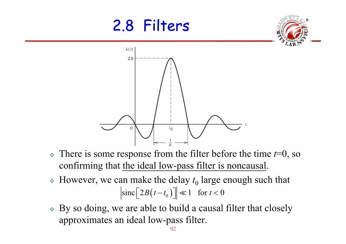
◊ There is some response from the filter before the time t=0, so confirming that the ideal low-pass filter is noncausal.H k th d l t l h h th t◊ However, we can make the delay t0 large enough such that

B d i bl b ild l fil h l l( )0sinc 2 1 for 0B t t t⎡ ⎤− <⎣ ⎦

92

◊ By so doing, we are able to build a causal filter that closely approximates an ideal low-pass filter.


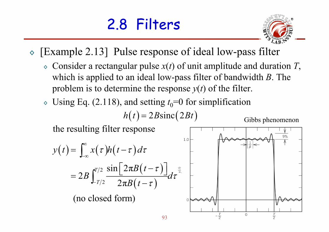
◊ [Example 2.13] Pulse response of ideal low-pass filterC id t l l ( ) f it lit d d d ti T◊ Consider a rectangular pulse x(t) of unit amplitude and duration T, which is applied to an ideal low-pass filter of bandwidth B. The problem is to determine the response y(t) of the filterproblem is to determine the response y(t) of the filter.

◊ Using Eq. (2.118), and setting t0=0 for simplification( ) ( )2 sinc 2h t B Bt=

the resulting filter response ( ) ( )2 sinc 2h t B Bt= Gibbs phenomenon

( ) ( ) ( )( )2 sin 2πT

y t x h t d

B t

τ τ τ

τ

∞

−∞= −

⎡ ⎤−⎣ ⎦

∫( )

( )2

2

sin 2π2

2π( l d f )

T

T

B tB d

B tτ

ττ−

⎡ ⎤−⎣ ⎦=−∫

93

(no closed form)

2.8 Filters2.8 Filters◊ Design of Filters

◊ Design of filters is usually carried out in the frequency domain◊ Design of filters is usually carried out in the frequency domain. There are two basic steps:◊ The approximation of a prescribed frequency response(i.e. amplitude pp p q y p ( p

response, phase response, or both) by a realizable transfer function.◊ The realization of the approximating transfer function by a physical

devicedevice.

◊ For an approximating transfer function H( f ) to be physically realizable it must represent a stable systemrealizable, it must represent a stable system.

◊ Stability is defined here on the basis of the bounded input bounded output criterion described in Eq. (2.100).p q ( )

◊ In the following, we specify the corresponding condition for stability in terms of the transfer function.

94

y◊ The traditional approach is to replace j2π f with s.

2.8 Filters2.8 Filters◊ Design of Filters

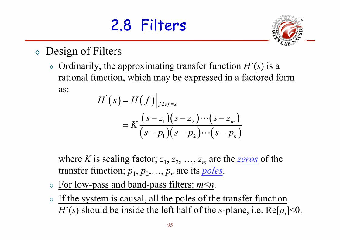
◊ Ordinarily the approximating transfer function H’(s) is a◊ Ordinarily, the approximating transfer function H (s) is a rational function, which may be expressed in a factored form as:

( ) ( )( )( ) ( )

'2π

1 2

j f sH s H f

s z s z s z==

− − −( )( ) ( )( )( ) ( )

1 2

1 2

m

n

s z s z s zK

s p s p s p=

− − −

where K is scaling factor; z1, z2, …, zm are the zeros of the transfer function; p1, p2,…, pn are its poles.; p1, p2, , pn p

◊ For low-pass and band-pass filters: m<n.◊ If the system is causal, all the poles of the transfer function

95

y , pH’(s) should be inside the left half of the s-plane, i.e. Re[pi]<0.


◊ Different Types of FiltersT l f ili f l filt B h fil◊ Two popular families of low-pass filters: Butterworth filtersand Chebyshev filters. All their zero are at s= ∞ and the poles are confined to the left half of the s-planeare confined to the left half of the s plane.

◊ Butterworth filter◊ The poles of the transfer function lie on a circle with origin as the center◊ The poles of the transfer function lie on a circle with origin as the center

and 2πB as the radius, where B is the 3-dB bandwidth of the filter.◊ Is said to have a maximally flat passband response.

◊ Chebyshev filter◊ The poles lie on an ellipse.

P id f t ll ff th B tt th filt b ll i i l i th◊ Provide faster roll-off than Butterworth filter by allowing ripple in the frequency response.

◊ Type 1 filters have ripple only in the passband.

96

yp pp y p◊ Type 2 filters have ripple only in the stopband and are seldom used.

2.8 Filters2.8 Filters◊ Comparison of the amplitude response of 6th order Butterworth

low-pass filter with that of 6th order Chebyshev filterlow pass filter with that of 6 order Chebyshev filter.

97

2.8 Filters2.8 Filters◊ A common alternative to both the Butterworth and Chebyshev filters

is the elliptic filter which has ripple in both the passband and theis the elliptic filter, which has ripple in both the passband and the stopband.

◊ Elliptic filter provide even faster roll-off for a given number of poles p p g pbut at the expense of ripple in both the passband and stopband.

◊ Butterworth filters are the simplest and elliptic filters are the more p pcomplicated to design in mathematical terms.

◊ The finite-duration impulse response (FIR) filter is often used in digital signal processing.

◊ The FIR filter is the equivalent of the tapped delay-line filter d ib d i h i idescribed in the previous section.

◊ The FIR filter has only zeros; it is thus inherently stable.

98

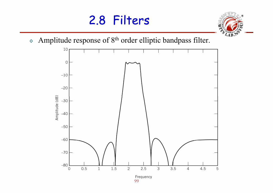
2.8 Filters2.8 Filters◊ Amplitude response of 8th order elliptic bandpass filter.

99

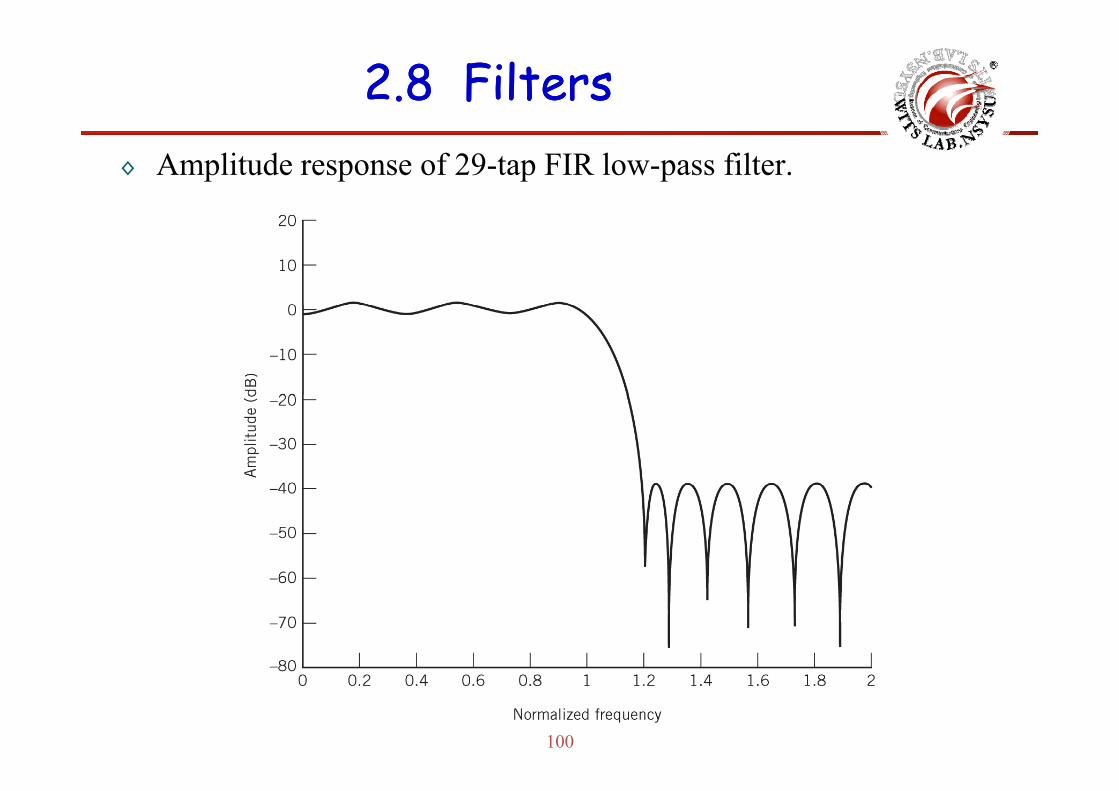
2.8 Filters2.8 Filters◊ Amplitude response of 29-tap FIR low-pass filter.

100

Chapter 2.9Chapter 2.9LowLow--Pass and BandPass and Band--Pass SignalsPass SignalsLowLow Pass and BandPass and Band Pass SignalsPass Signals


2.9 Low2.9 Low--Pass and BandPass and Band--Pass SignalsPass Signals

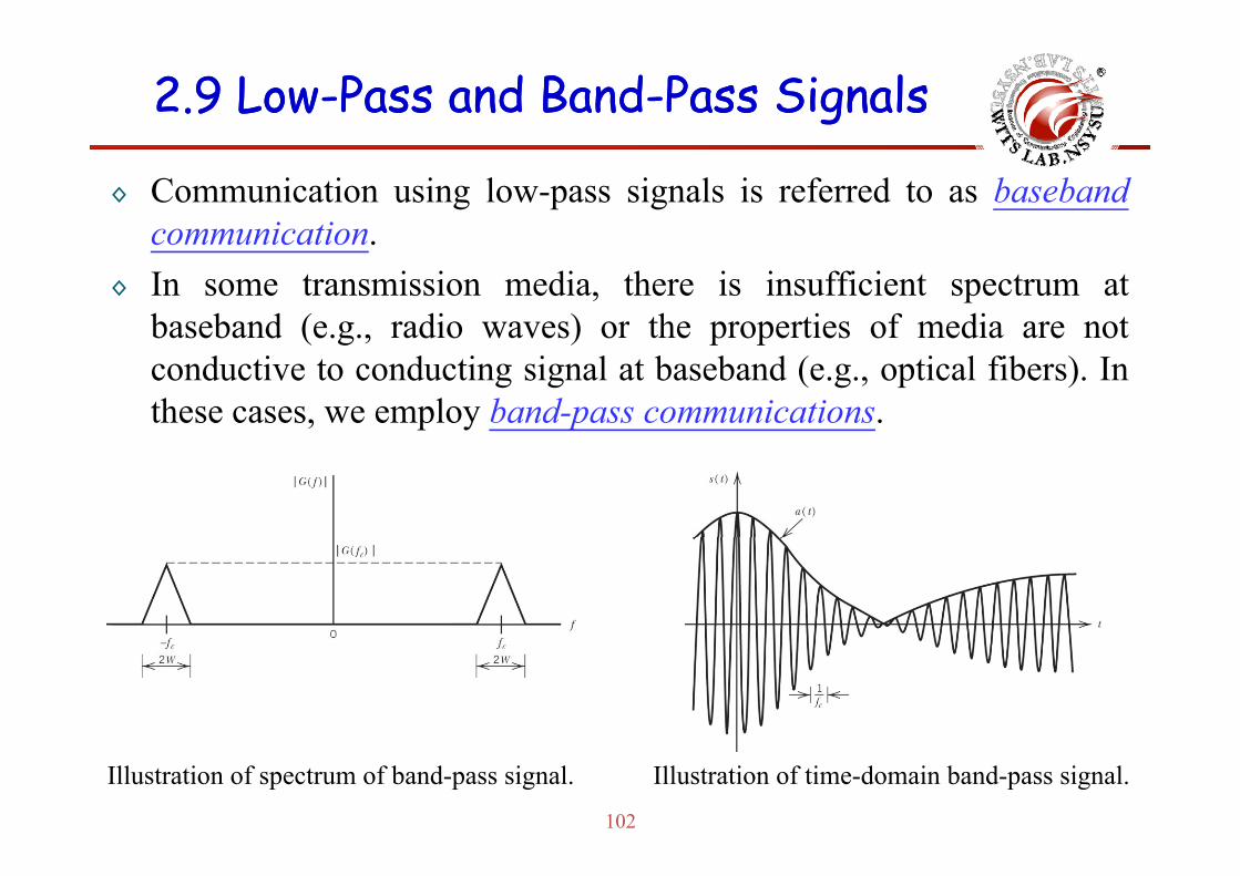
◊ Communication using low-pass signals is referred to as basebandcommunicationcommunication.

◊ In some transmission media, there is insufficient spectrum atbaseband (e.g., radio waves) or the properties of media are not( g , ) p pconductive to conducting signal at baseband (e.g., optical fibers). Inthese cases, we employ band-pass communications.

102

Illustration of spectrum of band-pass signal. Illustration of time-domain band-pass signal.


◊ Narrow-band signal: the bandwidth 2W is small compared to the carrier frequency f0carrier frequency f0.

◊ A real-valued band-pass signal g(t) with non-zero spectrum G( f ) in the vicinity of fc may be expressed in the form:y fc y p

( ) ( ) ( )cos 2π cg t a t f t tφ⎡ ⎤= +⎣ ⎦◊ a(t): envelope (non-negative)◊ : phase( )tφ

◊ Using the relationship cos(A+B)=cos(A)cos(B)-sin(A)sin(B)

( ) ( ) ( ) ( ) ( )cos 2π sin 2πg t g t f t g t f t= − (2 123)( ) ( ) ( ) ( ) ( )cos 2π sin 2πI c Q cg t g t f t g t f t= −

( ) ( ) ( ) ( ) ( ) ( )cos and sinI Qg t a t t g t a t tφ φ= =( ) ( ) ( )

( )

2 2I Qa t g t g t= +

⎛ ⎞

(2.123)

103

( ) ( ) ( ) ( ) ( ) ( )Q

in-phase of ( )g t quadrature of ( )g t ( ) ( )( )

1tan Q

I

g tt

g tφ − ⎛ ⎞

= ⎜ ⎟⎝ ⎠

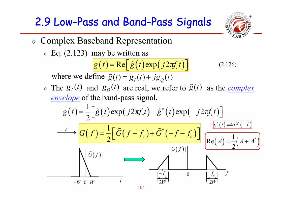
2.9 Low2.9 Low--Pass and BandPass and Band--Pass SignalsPass Signals◊ Complex Baseband Representation

◊ Eq (2 123) may be written as◊ Eq. (2.123) may be written as

where we define( ) ( ) ( )Re exp 2π cg t g t j f t⎡ ⎤= ⎣ ⎦

( ) ( ) ( )g t g t jg t= +

(2.126)

where we define ◊ The and are real, we refer to as the complex

envelope of the band-pass signal.

( ) ( ) ( )I Qg t g t jg t= +( )Ig t ( )Qg t ( )g t

envelope of the band pass signal.

( ) ( ) ( ) ( ) ( )1 exp 2π exp 2π2 c cg t g t j f t g t j f t∗⎡ ⎤= + −⎣ ⎦

( ) ( )G f∗ ∗

( ) ( ) ( )*12 c cG f G f f G f f⎡ ⎤= − + − −⎣ ⎦

F⎯⎯→( ) ( )*1Re

2A A A= +

( ) ( )g t G f∗ ∗ −

( ) ( )2( )| |G f

( )| |G f

104WW− 0 f

cfcf−

2W2W0 f


◊ [Example 2.14] PF pulse (continued) – read by yourselfT d t i th l l f th RF l◊ To determine the complex envelope of the RF pulse

( ) ( )rect cos 2π ctg t A f t⎛ ⎞= ⎜ ⎟

⎝ ⎠◊ Assume fcT>>1, so that g(t) is narrow-band

( ) ( )cg fT⎜ ⎟⎝ ⎠

( ) ( )Re rect exp 2π ctg t A j f tT

⎡ ⎤⎛ ⎞= ⎜ ⎟⎢ ⎥⎝ ⎠⎣ ⎦the complex envelope is

( ) rect tg t AT⎛ ⎞= ⎜ ⎟⎝ ⎠and the envelope equals

( )T⎜ ⎟⎝ ⎠

( ) ( ) t tt t A ⎛ ⎞⎜ ⎟

105

( ) ( ) recta t g t AT

= = ⎜ ⎟⎝ ⎠

Chapter 2.10Chapter 2.10BandBand--Pass SystemsPass SystemsBandBand Pass SystemsPass Systems


2.102.10 BandBand--Pass SystemsPass Systems◊ Summaries of low-pass systems:

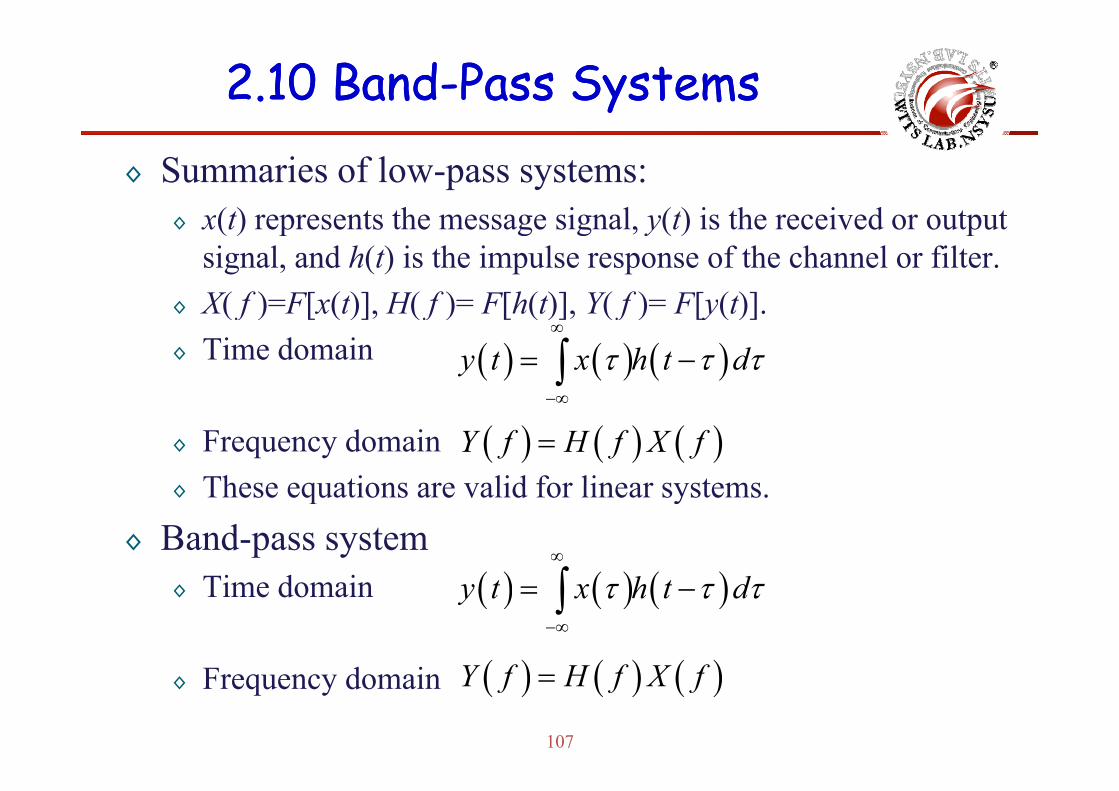
x(t) represents the message signal y(t) is the received or output◊ x(t) represents the message signal, y(t) is the received or output signal, and h(t) is the impulse response of the channel or filter.

◊ X( f )=F[x(t)] H( f )= F[h(t)] Y( f )= F[y(t)]◊ X( f )=F[x(t)], H( f )= F[h(t)], Y( f )= F[y(t)].◊ Time domain ( ) ( ) ( )y t x h t dτ τ τ

∞

∞

= −∫◊ Frequency domain◊ These equations are valid for linear systems

−∞

( ) ( ) ( )Y f H f X f=◊ These equations are valid for linear systems.

◊ Band-pass systemi d i ( ) ( ) ( )

∞

∫◊ Time domain ( ) ( ) ( )y t x h t dτ τ τ−∞

= −∫

( ) ( ) ( )f f f

107

◊ Frequency domain ( ) ( ) ( )Y f H f X f=

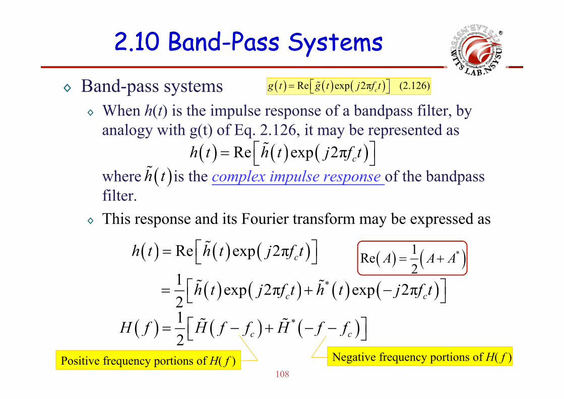
2.102.10 BandBand--Pass SystemsPass Systems◊ Band-pass systems

When h(t) is the impulse response of a bandpass filter by( ) ( ) ( )Re exp 2π (2.126)cg t g t j f t⎡ ⎤= ⎣ ⎦

◊ When h(t) is the impulse response of a bandpass filter, by analogy with g(t) of Eq. 2.126, it may be represented as

( ) ( ) ( )Re exp 2πh t h t j f t⎡ ⎤= ⎣ ⎦where is the complex impulse response of the bandpassfilter.

( ) ( ) ( )Re exp 2π ch t h t j f t⎡ ⎤= ⎣ ⎦( )h t

filter.◊ This response and its Fourier transform may be expressed as

( ) ( ) ( )h h f⎡ ⎤ 1( ) ( ) ( )

( ) ( ) ( ) ( )*

Re exp 2π

1 exp 2π exp 2π

ch t h t j f t

h t j f t h t j f t

⎡ ⎤= ⎣ ⎦

⎡ ⎤= +⎣ ⎦

( ) ( )*1Re2

A A A= +

( ) ( ) ( ) ( ) exp 2π exp 2π2 c ch t j f t h t j f t⎡ ⎤= + −⎣ ⎦　

( ) ( ) ( )*12 c cH f H f f H f f⎡ ⎤= − + − −⎣ ⎦

108

( ) ( ) ( )2 c cf f f f f⎣ ⎦

Positive frequency portions of H( f ) Negative frequency portions of H( f )

2.102.10 BandBand--Pass SystemsPass Systems

◊ Since is low-pass limited to | f |<B, we can obtain( )H f

( ) ( )2 , 00, 0c

H f fH f f

f⎧ >

− = ⎨<⎩ , f⎩

( )0, 0f

H f f>⎧

− − = ⎨

◊ This low-pass filter response is the frequency-domain equivalent

( ) ( )*2 , 0cH f fH f f

= ⎨ <⎩p p q y q

of the complex impulse response of the filter.◊ The output y(t) is also a band-pass signal:

( ) ( ) ( )Re exp 2 cy t y t j f tπ⎡ ⎤= ⎣ ⎦

109

where is the complex envelope of y(t).( )y t


( ) ( ) ( )Y f H f X f=

( ) ( ) ( ) ( )* *1 12 2c c c cH f f H f f X f f X f f⎡ ⎤ ⎡ ⎤= − + − − × − + − −⎣ ⎦ ⎣ ⎦

⎡ ⎤( ) ( ) ( ) ( )* *1 1 12 2 2c c c cH f f X f f H f f X f f⎡ ⎤= − − + − − − −⎢ ⎥⎣ ⎦

h

( ) ( )*12 c cY f f Y f f⎡ ⎤= − + − −⎣ ⎦

( ) ( ) ( )1

( ) ( )( ) ( )

*

*=c c

c c

H f f X f f

H f f X f f

− − −

− − −where ( ) ( ) ( )1

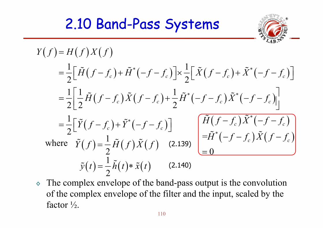
2Y f H f X f=

( ) ( ) ( )1y t h t x t= ∗

( ) ( )0

c cf f f f=

(2 140)

(2.139)

◊ The complex envelope of the band-pass output is the convolution f th l l f th filt d th i t l d b th

( ) ( ) ( )2

y t h t x t= ∗ (2.140)

110

of the complex envelope of the filter and the input, scaled by the factor ½.

2.102.10 BandBand--Pass SystemsPass Systems◊ The analysis of a band-pass system is complicated due to the

multiplying factors cos(2πfct) and sin(2πfct).p y g ( fc ) ( fc )◊ The significance of Eq. (2.140) is that, we need only concern the

low-pass functions, ( ) ( ) ( ), , and .x t h t y tp◊ In other words, the analysis of a band-pass system is replaced by

an equivalent but much simpler low-pass analysis that completely

( ) ( ) ( )

retains the essence of the filtering process.

13

( ) ( ) ( )12

y t h t x t= ∗

1112

2


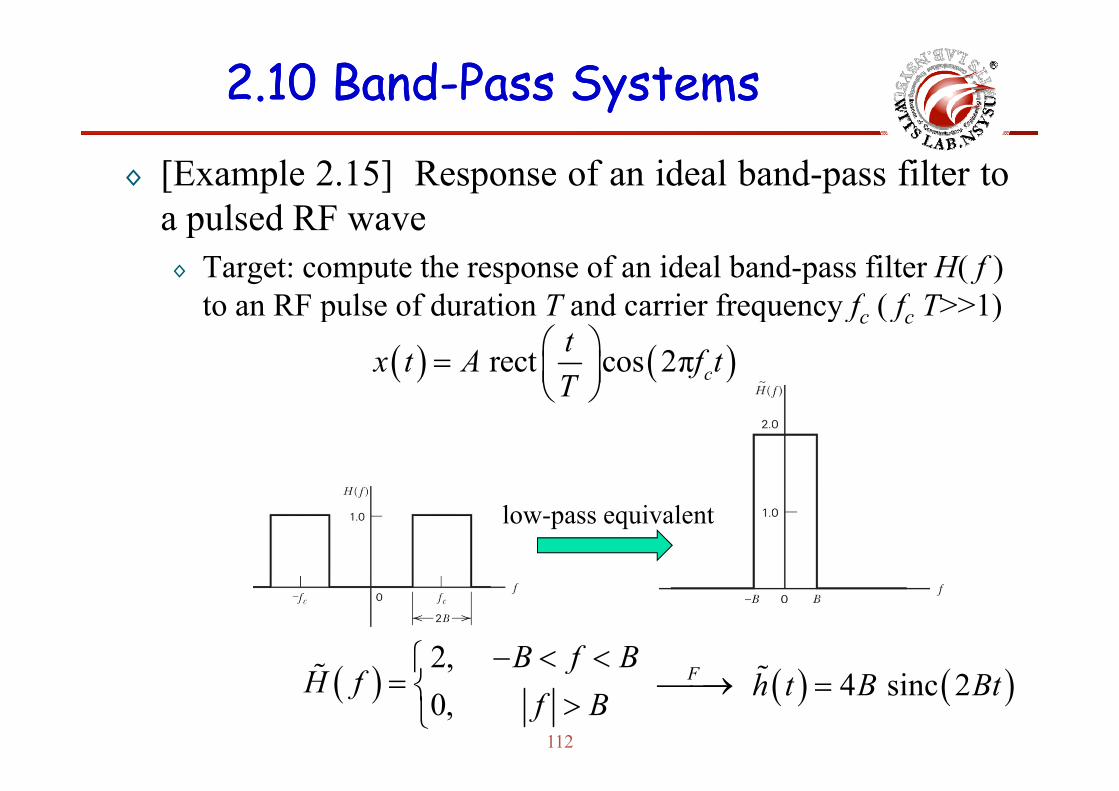
◊ [Example 2.15] Response of an ideal band-pass filter toa pulsed RF wavea pulsed RF wave◊ Target: compute the response of an ideal band-pass filter H( f )

to an RF pulse of duration T and carrier frequency f ( f T>>1)to an RF pulse of duration T and carrier frequency fc ( fc T>>1)

( ) ( ) rect cos 2π ctx t A f tT⎛ ⎞= ⎜ ⎟⎝ ⎠T⎝ ⎠

low-pass equivalent

2, B f B− < <⎧

112

( )2, 0,

B f BH f

f B< <⎧

= ⎨ >⎩( ) ( )4 sinc 2h t B Bt=F⎯⎯→


( ) ( )t⎛ ⎞( ) ( )rect cos 2π ctx t A f tT⎛ ⎞= ⎜ ⎟⎝ ⎠

( ) t tA ⎛ ⎞⎜ ⎟

low-pass equivalent( ) rectx t A

T⎛ ⎞= ⎜ ⎟⎝ ⎠

( ) ( ) ( )1 (no closed form)2

y t h t x t⇒ = ∗

113

Chapter 2.11Chapter 2.11Phase and Group DelayPhase and Group DelayPhase and Group DelayPhase and Group Delay


2.112.11 Phase and Group DelayPhase and Group Delay

◊ Whenever a signal is transmitted through a dispersive (frequency-selective) device such as a filter or communication channel someselective) device such as a filter or communication channel, some delay is introduced into the output signal in relation to the input signal.g

◊ In an ideal filter, the phase response varies linearly with frequency inside the passband of the filter, in which case the filter introduces a constant delay.

◊ Question: what if the phase response of the filter is nonlinear?◊ Signal Models: assume that a steady sinusoidal signal at frequency fc is

transmitted through a dispersive channel that has a total phase-shift of β( fc).◊ Phase delay of the channel: β( f )/2 πf [sec] is the time taken by the received◊ Phase delay of the channel: β( fc)/2 πfc [sec] is the time taken by the received

signal phasor to sweep out this phase lag.

◊ Phase delay is not necessarily the true signal delay.

115

y y g y◊ The true signal delay is represented by the envelope or group delay.


◊ Assume that the dispersive channel is described by the transfer function: ( ) ( )⎡ ⎤function:

where K is a constant the phase β( f ) is a nonlinear function of

( ) ( )expH f K j fβ⎡ ⎤= ⎣ ⎦

where K is a constant the phase β( f ) is a nonlinear function of frequency.

◊ The input signal x(t) consists of a narrow-band signal:◊ The input signal x(t) consists of a narrow-band signal:

where m(t) is a low pass (information bearing) signal with its( ) ( ) ( )cos 2π cx t m t f t=

where m(t) is a low-pass (information-bearing) signal with its spectrum limited to the frequency interval | f | ≦ W. Assume fc >> W.

◊ By using the Taylor series about the point f=f and retaining only the◊ By using the Taylor series about the point f fc and retaining only the first two terms:

( ) ( ) ( ) ( )β f∂ ( )

Taylor series at cf f=

116

( ) ( ) ( ) ( )ββ β

cc c f f

ff f f f

f =

∂+ −

∂( ) ( ) ( )

0

β!

nnc

cn

ff f

n

∞

=

−∑


◊ Define phase delay: ( )2

cp

ff

βτ

π= −

◊ Define group delay:( )1

2 cg f f

ff

βτ

π =

∂= −

∂

2 cfπ

2 fπ ∂

( ) ( ) ( ) ( ) ( ) ( )2 2cc c f f c p c g

ff f f f f f f f

fβ

β β β π τ π τ=

∂+ − ⇒ − − −

∂◊ The transfer function of the channel takes the form:

f∂

( ) ( )2 2H f K j f j f f⎡ ⎤

◊ Equivalent low-pass filter

( ) ( )exp 2 2c p c gH f K j f j f fπ τ π τ⎡ ⎤− − −⎣ ⎦( ) ( )2 , 0

0, 0cH f f

H f ff

⎧ >− = ⎨

<⎩

◊ Low pass complex envelope and its Fourier transform:

( ) ( )2 exp 2 2c p gH f K j f j fπ τ π τ− −0, 0f <⎩

117

◊ Low-pass complex envelope and its Fourier transform:( ) ( ) ( ) ( ) ( ), x t m t X f M f F m t⎡ ⎤= = ⎣ ⎦


◊ The Fourier transform of the complex envelope of the received signal: 1signal:

( ) ( ) ( )

( ) ( ) ( )

1 (2.139)2

Y f H f X f=

◊ The term exp(-j2πfτg)M( f ) represents the Fourier transform of the

( ) ( ) ( )exp 2 exp 2c p gK j f j f M fπ τ π τ− −

p( j f g) ( f ) pdelayed signal m(t-τg).

◊ Complex envelope of the received signal:

R i d i l

( ) ( ) ( )exp 2 c p gy t K j f m tπ τ τ− −

◊ Received signal:( ) ( ) ( )

( ) ( )Re exp 2 cy t y t j f tπ⎡ ⎤= ⎣ ⎦

⎡ ⎤

118

( ) ( )cos 2g c pKm t f tτ π τ⎡ ⎤= − −⎣ ⎦

2.112.11 Phase and Group DelayPhase and Group Delay◊ The sinusoidal carrier wave cos(2πfct) is delay by τp seconds, hence τ represents the phase delay Sometimes τ is also referred to as theτp represents the phase delay. Sometimes, τp is also referred to as the carrier delay.

◊ The envelope m(t) is delayed by τg seconds; hence, τg represents the p ( ) y y g ; , g penvelope or group delay.

◊ τg is related to the slope of the phase β( f ), measured at f=fc.◊ When the phase response β( f ) varies linearly with frequency, the p p β( f ) y q y,

signal is delayed but undistorted.◊ When this linear condition is violated, we get group delay distortion.

119

Chapter 2.12Chapter 2.12Sources of InformationSources of InformationSources of InformationSources of Information


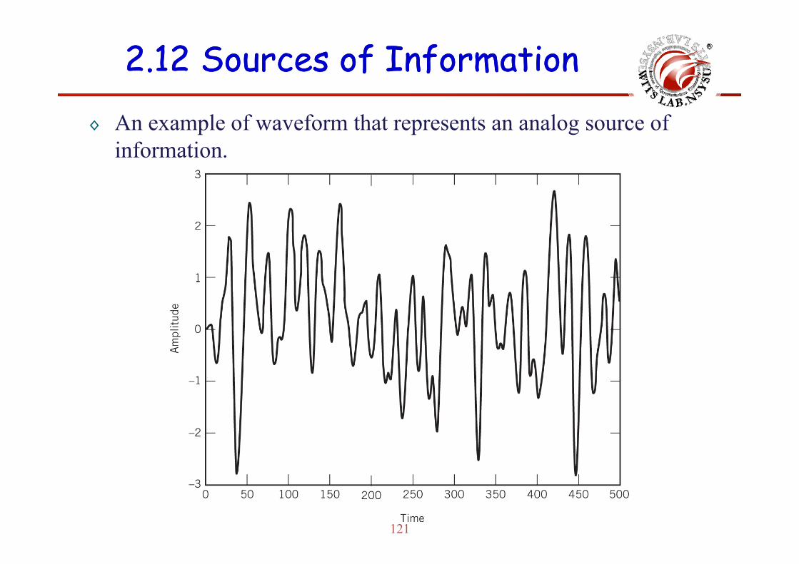
2.122.12 SourcesSources ofof InformationInformation◊ An example of waveform that represents an analog source of

informationinformation.

121

2.122.12 SourcesSources ofof InformationInformation◊ Some source are digital in the sense that the information can be

naturally represented as a sequence of zeros and onesnaturally represented as a sequence of zeros and ones.◊ The digital waveform can be represented as:

( ) ( )0

K

kk

g t b p t kT=

= −∑

Figure 2.38 (a)rectangular pulse shape

Figure 2.38 (b)non-rectangular pulse shape

122

comm-02-fourier theory and communication signals

Documents

inverse fourier transform

fourier transformchapter

communication fourier

transmission of signals

time function

d i h d i

function gt

functions of time