Combining weak lensing and SNIa

using CFHTLS-Wide and SNLS

Martin Kilbinger (IAP)

Ismael Tereno (AIfA) · Karim Benabed (IAP) · Pierre Astier (Jusieu) · Julien Guy (Jusieu) · Yannick Mellier (IAP) · Liping

Fu (IAP) · L. van Waerbeke (UBC) · H. Hoekstra (UVic)SNLS · Terapix

The SNLS sample

1st year data: 71 distant + 44 nearby SNIa

Imaging: CFHTLS (4 sq deg Deep fields)Spectroscopy: VLT, Gemini, Keck

3rd year data in prep.

40 P. Astier et al. (SNLS Collaboration): SNLS 1st year data set

5.4. Cosmological fits

From the fits to the light-curves (Sect. 5.1), we computed arest-frame-B magnitude, which, for perfect standard candles,should vary with redshift according to the luminosity distance.This rest-frame-B magnitude refers to observed brightness, andtherefore does not account for brighter-slower and brighter-bluer correlations (see Guy et al. 2005 and references therein).As a distance estimator, we use:

µB = m!B " M + !(s " 1) " "cwhere m!B, s and c are derived from the fit to the light curves,and !, " and the absolute magnitude M are parameters whichare fitted by minimizing the residuals in the Hubble diagram.The cosmological fit is actually performed by minimizing:

#2 =!

objects

"µB " 5 log10(dL($, z)/10 pc)

#2

%2(µB) + %2int

,

where $ stands for the cosmological parameters that define thefitted model (with the exception of H0), dL is the luminos-ity distance, and %int is the intrinsic dispersion of SN abso-lute magnitudes. We minimize with respect to $, !, " and M.Since dL scales as 1/H0, only M depends on H0. The definitionof %2(µB), the measurement variance, requires some care. First,one has to account for the full covariance matrix of m!B, s and cfrom the light-curve fit. Second, %(µB) depends on ! and ";minimizing with respect to them introduces a bias towards in-creasing errors in order to decrease the #2, as originally notedin Tripp (1998). When minimizing, we therefore fix the val-ues of ! and " entering the uncertainty calculation and updatethem iteratively. %(µB) also includes a peculiar velocity con-tribution of 300 km s"1. %int is introduced to account for the“intrinsic dispersion” of SNe Ia. We perform a first fit with aninitial value (typically 0.15 mag), and then calculate the %int

required to obtain a reduced #2 = 1. We then refit with thismore accurate value. We fit 3 cosmologies to the data: a ! cos-mology (the parameters being"M and"!), a flat! cosmology(with a single parameter "M), and a flat w cosmology, where wis the constant equation of state of dark energy (the parametersare "M and w).

The Hubble diagram of SNLS SNe and nearby data isshown in Fig. 4, together with the best fit ! cosmology fora flat Universe. Two events lie more than 3% away from theHubble diagram fit: SNLS-03D4au is 0.5 mag fainter than thebest-fit and SNLS-03D4bc is 0.8 mag fainter. Although, keep-ing or removing these SNe from the fit has a minor e#ect onthe final result, they were not kept in the final cosmology fits(since they obviously depart from the rest of the population)which therefore make use of 44 nearby objects and 71 SNLSobjects.

The best-fitting values of ! and " are ! = 1.52 ± 0.14and " = 1.57 ± 0.15, comparable with previous works usingsimilar distance estimators (see for example Tripp 1998). Asdiscussed by several authors (see Guy et al. (2005) and ref-erences therein), the value of " does di#er considerably fromRB = 4, the value expected if color were only a#ected bydust reddening. This discrepancy may be an indicator of intrin-sic color variations in the SN sample (e.g. Nobili et al. 2003),

SN Redshift0.2 0.4 0.6 0.8 1

Bµ

34

36

38

40

42

44

)=(0.26,0.74)!",m"(

)=(1.00,0.00)!",m"(

SNLS 1st Year

SN Redshift0.2 0.4 0.6 0.8 1

) 0 H

-1 c

L (

d10

- 5

log

Bµ

-1

-0.5

0

0.5

1

Fig. 4. Hubble diagram of SNLS and nearby SNe Ia, with various cos-mologies superimposed. The bottom plot shows the residuals for thebest fit to a flat ! cosmology.

and/or variations in RB. For the absolute magnitude M, we ob-tain M = "19.31 ± 0.03 + 5 log10 h70.

The parameters !, " and M are nuisance parameters in thecosmological fit, and their uncertainties must be accounted forin the cosmological error analysis. The resulting confidencecontours are shown in Figs. 5 and 6, together with the productof these confidence estimates with the probability distributionfrom baryon acoustic oscillations (BAO) measured in the SDSS(Eq. (4) in Eisenstein et al. 2005). We impose w = "1 for the("M,"!) contours, and "k = 0 for the ("M, w) contours. Notethat the constraints from BAO and SNe Ia are quite comple-mentary. The best-fitting cosmologies are given in Table 3.

Using Monte Carlo realizations of our SN sample, wechecked that our estimators of the cosmological parametersare unbiased (at the level of 0.1%), and that the quoteduncertainties match the observed scatter. We also checkedthe field-to-field variation of the cosmological analysis. Thefour "M values (one for each field, assuming "k = 0) arecompatible at 37% confidence level. We also fitted separatelythe Ia and Ia* SNLS samples and found results compatible atthe 75% confidence level.

[Astier et al. 2006]

Light-curve fitting

Fits to two or more bands simultaneously using SALT [Guy et al. 2005]

Returns rest-frame magnitude , stretch s and color c

m!B

P. Astier et al. (SNLS Collaboration): SNLS 1st year data set 35

JD 2450000+3100 3150 3200

Flux

Mg

Mi

Mr

Mz

0

SNLS-04D3fk

Fig. 1. Observed light-curves points of the SN Ia SNLS-04D3fkin gM, rM, iM and zM bands, along with the multi-color light-curvemodel (described in Sect. 5.1). Note the regular sampling of the ob-servations both before and after maximum light. With a SN redshiftof 0.358, the four measured pass-bands lie in the wavelength rangeof the light-curve model, defined by rest-frame U to R bands, andall light-curves points are therefore fitted simultaneously with onlyfour free parameters (photometric normalization, date of maximum, astretch and a color parameter).

The !2n contribution of every individual image is evaluated, and

outliers>5" (due to, for example, unidentified cosmic rays) arediscarded; this cut eliminates 1.4% of the measurements on av-erage. The covariance of the per-night fluxes is then extracted,and normalized so that the minimum !2

n per degree of free-dom is 1. This translates into an “e!ective” flux uncertaintyderived from the scatter of repeated observations rather thanfrom first principles. If the only source of noise (beyond photonstatistics) were pixel correlations introduced by image resam-pling, we would expect an average !2

n/Nd.o.f. of 1.25, as all fluxvariances are on average under-estimated by 25%. Our averagevalue is 1.55; hence we conclude that our photometric uncer-tainties are only !12% (

"(1.55/1.25) # 1) larger than photon

statistics, leaving little margin for drastic improvement.Table 2 summarizes the statistics of the di!erential pho-

tometry fits in each filter. The larger values of !2n/Nd.o.f. in iM

and zM probably indicate contributions from residual fringes.Examples of SNe Ia light-curves points are presented in Figs. 1and 2 showing SNe at z = 0.358 and z = 0.91 respectively.Also shown on these figures are the results of the light-curvesfits described in Sect. 5.1.

The next section discusses how accurately the SN fluxescan be extracted from the science frames relative to nearbyfield stars, i.e. how well the method assigns magnitudes to SNe,given magnitudes of the field stars which are used for photo-metric calibration, called tertiary standards hereafter.

3.4. Photometric alignment of supernovae relativeto tertiary standards

The SN flux measurement technique of Sect. 3.2 deliversSN fluxes on the same photometric scale as the reference im-age. In this Section, we discuss how we measure ratios of theSN fluxes to those of the tertiary standards (namely stars in the

JD 2450000+3100 3150 3200

Flux

Mg

Mi

Mr

Mz

0

SNLS-04D3gx

Fig. 2. Observed light-curves points of the SN Ia SNLS-04D3gx at z =0.91. With a SN redshift of 0.91, only two of the measured pass-bandslie in the wavelength range of the light-curve model, defined by rest-frame U to R bands, and are therefore used in the fit (shown as solidlines). Note the excellent quality of the photometry at this high redshiftvalue. Note also the clear signal observed in rM and even in gM, whichcorrespond to central wavelength of respectively # ! 3200 Å and # !2500 Å in the SN rest-frame.

Table 2. Average number of images and nights per band for eachSNLS light-curve. Note that there is less data in gM and zM. The !2

n col-umn refers to the last fit that imposes equal fluxes on a given night. Theexpected value is 1.25 (due to pixel correlations), so we face a mod-erate scatter excess of about 12% over photon statistics. The largervalues in iM and zM indicate that fringes play a role in this excess. Thelast column displays the average wavelength of the e!ective filtersin Å.

Band Average nb. Average nb. !2n Central

of images of epochs per d.o.f. wavelength

gM 40 9.8 1.50 4860

rM 75 14.4 1.40 6227

iM 100 14.8 1.63 7618

zM 60 7.9 1.70 8823

SNLS fields). The absolute flux calibration of the tertiary stan-dards themselves is discussed in Sect. 4.

The image model that we use to measure the SN fluxes(Eq. (1)) can also be adapted to fit the tertiary standards bysetting the “underlying galaxy model” to zero. We measurethe fluxes of field stars by running the same simultaneous fitto the images used for the supernovae, but without the “zero-flux” images, and without an underlying galaxy. As this fittingtechnique matches that used for the SNe as closely as possible,most of the systematics involved (such as astrometric align-ment residuals, PSF model uncertainties, and the convolutionkernel modeling) cancel in the flux ratios.

For each tertiary standard (around 50 per CCD), we ob-tain one flux for each image (as done for the SNe), expressedin the same units. From the magnitudes of these fitted stars,we can extract a photometric zero point for the PSF photom-etry for every star on every image, which should be identicalwithin measurement uncertainties. Several systematic checkswere performed to search for trends in the fitted zero-points

z=0.358

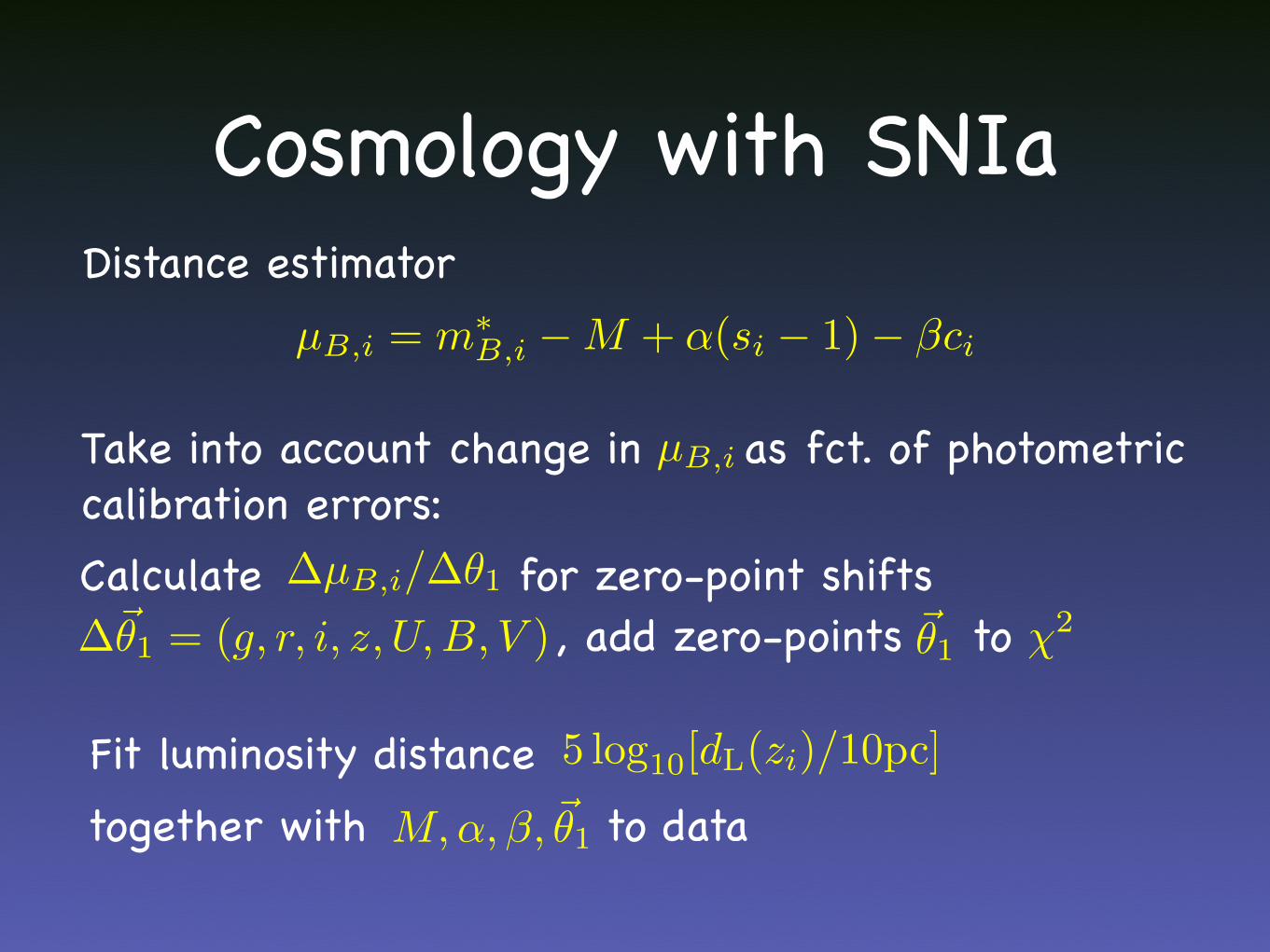
Cosmology with SNIaDistance estimator

together with to dataFit luminosity distance 5 log10[dL(zi)/10pc]

µB,i = m!B,i !M + !(si ! 1)! "ci

Take into account change in as fct. of photometric calibration errors:

µB,i

!µB,i/!!1Calculate for zero-point shifts, add zero-points to !2!"1

M,!, ", #$1

!!"1 = (g, r, i, z, U, B, V )

Influence of zero-pointsw = -1 flat

solid: Δzp≠0, dashed: Δzp=0

Bias from zero-points?

w = -1

flat

Correlations between systematic and cosmological parameters

= ΔU

= Δz

= ΔV

Most cases: no correlation Strong correlationµB,i = m!

B,i !M + !(si ! 1)! "ci

c = (B ! V )Bmax + 0.057

Lensing + n(z) + SNIa:first results

40 P. Astier et al. (SNLS Collaboration): SNLS 1st year data set

5.4. Cosmological fits

From the fits to the light-curves (Sect. 5.1), we computed arest-frame-B magnitude, which, for perfect standard candles,should vary with redshift according to the luminosity distance.This rest-frame-B magnitude refers to observed brightness, andtherefore does not account for brighter-slower and brighter-bluer correlations (see Guy et al. 2005 and references therein).As a distance estimator, we use:

µB = m!B " M + !(s " 1) " "cwhere m!B, s and c are derived from the fit to the light curves,and !, " and the absolute magnitude M are parameters whichare fitted by minimizing the residuals in the Hubble diagram.The cosmological fit is actually performed by minimizing:

#2 =!

objects

"µB " 5 log10(dL($, z)/10 pc)

#2

%2(µB) + %2int

,

where $ stands for the cosmological parameters that define thefitted model (with the exception of H0), dL is the luminos-ity distance, and %int is the intrinsic dispersion of SN abso-lute magnitudes. We minimize with respect to $, !, " and M.Since dL scales as 1/H0, only M depends on H0. The definitionof %2(µB), the measurement variance, requires some care. First,one has to account for the full covariance matrix of m!B, s and cfrom the light-curve fit. Second, %(µB) depends on ! and ";minimizing with respect to them introduces a bias towards in-creasing errors in order to decrease the #2, as originally notedin Tripp (1998). When minimizing, we therefore fix the val-ues of ! and " entering the uncertainty calculation and updatethem iteratively. %(µB) also includes a peculiar velocity con-tribution of 300 km s"1. %int is introduced to account for the“intrinsic dispersion” of SNe Ia. We perform a first fit with aninitial value (typically 0.15 mag), and then calculate the %int

required to obtain a reduced #2 = 1. We then refit with thismore accurate value. We fit 3 cosmologies to the data: a ! cos-mology (the parameters being"M and"!), a flat! cosmology(with a single parameter "M), and a flat w cosmology, where wis the constant equation of state of dark energy (the parametersare "M and w).

The Hubble diagram of SNLS SNe and nearby data isshown in Fig. 4, together with the best fit ! cosmology fora flat Universe. Two events lie more than 3% away from theHubble diagram fit: SNLS-03D4au is 0.5 mag fainter than thebest-fit and SNLS-03D4bc is 0.8 mag fainter. Although, keep-ing or removing these SNe from the fit has a minor e#ect onthe final result, they were not kept in the final cosmology fits(since they obviously depart from the rest of the population)which therefore make use of 44 nearby objects and 71 SNLSobjects.

The best-fitting values of ! and " are ! = 1.52 ± 0.14and " = 1.57 ± 0.15, comparable with previous works usingsimilar distance estimators (see for example Tripp 1998). Asdiscussed by several authors (see Guy et al. (2005) and ref-erences therein), the value of " does di#er considerably fromRB = 4, the value expected if color were only a#ected bydust reddening. This discrepancy may be an indicator of intrin-sic color variations in the SN sample (e.g. Nobili et al. 2003),

SN Redshift0.2 0.4 0.6 0.8 1

Bµ

34

36

38

40

42

44

)=(0.26,0.74)!",m"(

)=(1.00,0.00)!",m"(

SNLS 1st Year

SN Redshift0.2 0.4 0.6 0.8 1

) 0 H

-1 c

L (

d10

- 5

log

Bµ

-1

-0.5

0

0.5

1

Fig. 4. Hubble diagram of SNLS and nearby SNe Ia, with various cos-mologies superimposed. The bottom plot shows the residuals for thebest fit to a flat ! cosmology.

and/or variations in RB. For the absolute magnitude M, we ob-tain M = "19.31 ± 0.03 + 5 log10 h70.

The parameters !, " and M are nuisance parameters in thecosmological fit, and their uncertainties must be accounted forin the cosmological error analysis. The resulting confidencecontours are shown in Figs. 5 and 6, together with the productof these confidence estimates with the probability distributionfrom baryon acoustic oscillations (BAO) measured in the SDSS(Eq. (4) in Eisenstein et al. 2005). We impose w = "1 for the("M,"!) contours, and "k = 0 for the ("M, w) contours. Notethat the constraints from BAO and SNe Ia are quite comple-mentary. The best-fitting cosmologies are given in Table 3.

Using Monte Carlo realizations of our SN sample, wechecked that our estimators of the cosmological parametersare unbiased (at the level of 0.1%), and that the quoteduncertainties match the observed scatter. We also checkedthe field-to-field variation of the cosmological analysis. Thefour "M values (one for each field, assuming "k = 0) arecompatible at 37% confidence level. We also fitted separatelythe Ia and Ia* SNLS samples and found results compatible atthe 75% confidence level.

MCMC

1d marginals

Other systematics

Intrinsic velocity dispersion: discard SNIa @ z<0.015, add σint = 0.15 to errors

Malmquist bias: average brightness = fct(z), affects reconstructed distance. Has to be taken into account for w(z)!

Gravitational lensing, extinction, k-correction, SN evolution

Next steps

Add WMAP3 data

Go beyond w=const. Need specific model, e.g. Quintessence

Go beyond MCMC for efficient+unbiased sampling of the posterior: Importance sampling, Population MonteCarlo (PMC)

Include shear systematics (shape measurements, photo-z’s)?