combining state-and-transition simulations and species distribution

Manuscript submitted to: Volume 2, Issue 2, 400-426.

AIMS Environmental Science DOI: 10.3934/environsci.2015.2.400

Received date 30 January 2015, Accepted date 13 April 2015, Published date 12 May 2015

Research article

Combining state-and-transition simulations and species distribution

models to anticipate the effects of climate change

Brian W. Miller 1, 2, *, Leonardo Frid 3, Tony Chang 4, Nathan Piekielek 5, Andrew J. Hansen 4 and Jeffrey T. Morisette 2, 6

1 Natural Resource Ecology Laboratory, Colorado State University, Fort Collins, CO, 80523-1499, USA

2 Department of the Interior North Central Climate Science Center, Fort Collins, CO, 80523-1499, USA

3 Apex Resource Management Solutions Ltd., Bowen Island, BC V0N 1G1, Canada 4 Montana State University, Bozeman, MT, 59717, USA 5 The Pennsylvania State University, University Park, PA, 16802, USA 6 U.S. Geological Survey, North Central Climate Science Center, Fort Collins, CO, 80526, USA

* Correspondence: [email protected]; Tel: +1-970-491-7659; Fax: +1-970-491-1965.

Abstract: State-and-transition simulation models (STSMs) are known for their ability to explore the combined effects of multiple disturbances, ecological dynamics, and management actions on vegetation. However, integrating the additional impacts of climate change into STSMs remains a challenge. We address this challenge by combining an STSM with species distribution modeling (SDM). SDMs estimate the probability of occurrence of a given species based on observed presence and absence locations as well as environmental and climatic covariates. Thus, in order to account for changes in habitat suitability due to climate change, we used SDM to generate continuous surfaces of species occurrence probabilities. These data were imported into ST-Sim, an STSM platform, where they dictated the probability of each cell transitioning between alternate potential vegetation types at each time step. The STSM was parameterized to capture additional processes of vegetation growth and disturbance that are relevant to a keystone species in the Greater Yellowstone Ecosystem—whitebark pine (Pinus albicaulis). We compared historical model runs against historical observations of whitebark pine and a key disturbance agent (mountain pine beetle, Dendroctonus ponderosae), and then projected the simulation into the future. Using this combination of correlative and stochastic simulation models, we were able to reproduce historical observations and identify key data gaps. Results indicated that SDMs and STSMs are complementary tools, and combining them is an effective way to account for the anticipated impacts of climate change, biotic interactions, and

401

AIMS Environmental Science Volume 2, Issue 2, 400-426.

disturbances, while also allowing for the exploration of management options.

Keywords: climate change; Greater Yellowstone Ecosystem; mountain pine beetle; spatially explicit simulation; ST-Sim; VisTrails:SAHM; whitebark pine

1. Introduction

There is a challenging dichotomy in the resource management community. On the one hand, there is a need to know and understand fundamental physical processes at a very specific and local level. On the other, there is also a need to know the larger context within which the system works. This is particularly true for integrating climate change into natural resource management practices. Ecological restoration and management actions require an understanding of local conditions (such as species competition, disturbance conditions, micro topography, and a given jurisdiction’s management options), but climate impacts are often measured and modeled at a coarser scale and imply the need to consider the wider landscape. Recent work has called for integrating various methods in order to overcome limitations of individual tools and the challenges associated with climate change adaptation [1].

Species distribution modeling (SDM) has proven useful for estimating the potential impacts of climate change and other abiotic factors on species distributions. Many SDMs are popular due to their ability to generate complex predictions without high computational requirements; however, there has been increasing recognition of the limitations of SDMs related to interspecific interactions, dispersal, equilibria, stochastic events, and fundamental niche space [2,3]. In addition to their inherent limitations, there are some specific questions that are not appropriate or possible within the framework of correlative modeling but may be of keen interest to natural resource managers. For example, what would happen to a species if the budget for a given restoration project was doubled or cut in half?

State-and-transition simulation models (STSMs) provide a spatial and quantitative framework to explore “what if” scenarios, which can be used to explore both management options and evaluate the sensitivity of the system to specific parameterizations or assumptions [4]. STSMs have been recognized as useful tools for incorporating the effects of multiple disturbances, biotic interactions, and management scenarios, but lack statistically robust techniques for relating climate data to species distributions. Together, STSMs and SDMs are well-equipped to account for the various facets of natural resource management challenges, at both regional and local scales, and combine them in a spatial simulation framework.

Our case study of whitebark pine in the Greater Yellowstone Ecosystem serves as a proof-of-concept for combining stochastic simulation models (STSMs) and correlative models (SDMs), and sets the stage for future exploration of management options. This research offers two novel contributions: 1) accounting for climate change and other dynamics through a combination of SDMs and STSMs; and 2) outlining an approach for validating STSMs based on recent developments in agent-based modeling, which remains an active area of exploration.

402


2. Background

2.1. Species distribution models

Species distribution models (SDMs) refer to a variety of empirical methods that associate species with the attributes of their preferred bioclimatic environment, also sometimes referred to as “habitat” [5,6]. SDMs evolved over the last several decades from our conceptual understanding of niche theory combined with the increased availability of geospatial datasets and geographic information systems with which to quantify bioclimatic attributes and their variation across space. SDMs typically represent individual species presence (and/or absence) at the spatial resolution of commonly available climate data (usually ~ 1 km or coarser) at temporal resolutions of decades or longer (often 30 year averages). More recently, interest in the ecological impacts of climate change has spurred rapid development and growth in application of SDMs because they are relatively easy to train on contemporary conditions and apply to projected future conditions. Future SDM projections often support commonly held assumptions about climate change and species extinctions and range shifts, although their temporal transferability (i.e., ability to be calibrated for one time period and make predictions for another) is rarely considered [7].

There are numerous challenges to producing actionable science using SDMs including that: they often represent unknown mechanistic relationships between species and their environments [8]; empirical methods do not always capture the direct effects of climate on species in ecologically meaningful ways [9]; there is often a mismatch of spatial and temporal resolution between SDMs and management action [10]; and SDMs rarely consider climate change impacts to communities of species and functional types whereas management is often charged with preserving assemblages of species and ecosystem function [11]. Numerous refinements of SDMs have been proposed [12]; however, the above challenges suggest that there remains a need to develop new methods that better produce scientific information that is useful to natural resource managers who are engaged in climate adaptation planning.

2.2. State-and-transition models

State-and-transition models originated as conceptual models that represented groups of vegetation communities and the shifts between them [13]. The definition of states often depends on the modeling objectives and data availability, but can generally be thought of as suites of vegetation communities that have distinct functional groups, ecosystem processes, and structure [14]. Transitions include natural events, management interventions, or a combination of both [15]. State-and-transition models are typically represented using box and arrow diagrams, in which boxes or nested boxes represent vegetation phases and states, and arrows represent the transitions between them.

These conceptual models remain at the heart of more recent quantitative computer-based state-and-transition models, or state-and-transition simulation models (STSMs, reviewed by Daniel and Frid [4]). In STSMs, transitions can be deterministic (e.g., growth, aging) or probabilistic (e.g., fire, invasion), and can be aspatial or spatially explicit. Spatially explicit STSMs are analogous to joint cellular automata-Markov models [16], hybrid Markov-cellular automaton models [17], and spatio-temporal Markov chains [18]. Bestelmeyer et al. [19] note that spatial context is important for

403


conceptual state-and-transition models because spatial dynamics such as contagion, feedbacks between patches, spatial patterns in historical legacies, and variation in soils, topography, and climate can all affect the likelihood and location of transitions. These spatial dynamics can similarly be incorporated into spatially explicit STSMs.

STSMs can be used to compare and evaluate different resource management scenarios [20-23], and can incorporate climate effects [24-28]. Here we present a novel approach to incorporating the effects of climate on vegetation into STSMs that is spatially explicit and based on correlative models of habitat suitability.

2.3. Study area

Whitebark pine (Pinus albicaulis) is an iconic member of the subalpine forest community in the western North American mountains and is highly valued for the ecosystem services it provides. It is considered a keystone species because it has strong influence on ecosystem properties. Whitebark pine (WBP) is able to tolerate the harsh conditions typical of mountainous terrain and creates forest in high-elevation locations that would otherwise be shrubs and herb. By colonizing open subalpine patches, it provides safe sites for subalpine fir (Abies lasiocarpa) and other species resulting in greater forest cover. In addition to providing habitat for many wildlife species the unusual reproductive strategy of producing large crops of cones with large nutritious seeds every few years provides a rich food source to the threatened Grizzly bear and other wildlife species. In addition to these positive effects on high-elevation ecosystems, the species has strong social values. The unique umbrella shape, large size, and grizzled appearance developed over its centuries-long lifespan evokes strong emotional appeal to people visiting these mountain haunts.

The Greater Yellowstone Ecosystem (GYE), which includes Yellowstone National Park, Grand Teton National Park, and a number of state and federally managed forests, is a mid- to high-latitude region in the Northern Rocky Mountains of western North America. Conifers are dominant in the range, with forest types composed of Pinus contorta, Abies lasiocarpa, Pseudotsuga menziesii, Pinus albicaulis, Juniperus scopulorum, Pinus flexis and Picea engelmannii, although the deciduous hardwood Populus tremuloides, is also wide spread. Plateaus and lowlands are dominated by species of Artemisia tridentata and open grasslands of mixed composition. The GYE study area encompasses 150,700 km2 with an elevational gradient from 522–4,206 m that represents 14 surrounding mountain ranges [29].

WBP is present in the GYE from below 2,100 m to nearly 3,300 m, an elevation range that spans the montane and subalpine zones [30]. WBP is subdominant to other conifer species in the lower portion of its distribution and is dominant in many locations at upper treeline [31]. The WBP population in the GYE has been particularly hard hit in recent years: in some areas whitebark pine mortality has exceeded 95% of cone bearing trees (DBH > 15 cm) [32] due to factors related to warming climate, mountain pine beetle (Dendroctonus ponderosae), and an exotic fungal pathogen (Cronartium ribicola) associated with white pine blister rust [33]. Beyond the current forest die-off, resource managers are concerned because the area of suitable habitat for WBP in the GYE is projected to decline dramatically in the coming century due to projected climate change [29,34,35,36]. Consequently, the US Fish and Wildlife Service listed the WBP on the U.S. candidate species list [37]. Yet questions remain as to how best to manage WBP under these various threats.

404


Figure 1. Study area, highlighting the approximate extent of the Greater Yellowstone Ecosystem.

3. Methods

3.1. Species distribution modeling

For the SDM portion of the research, we used the VisTrails:SAHM software package to preprocess data, select predictor variables, compare model algorithms, produce model diagnostics, and capture data and workflow provenance. VisTrails is a free open source scientific workflow software [38] that has been customized for SDM using a set of add-on tools that comprise the Software for Assisted Habitat Modeling (SAHM) [39].

Field observations of adult tree presences and absences were compiled from the Forest Inventory and Analysis (FIA) program, Whitebark/Limber Pine Information System [40], and long term monitoring plots established by the National Park Service Greater Yellowstone Inventory and Monitoring Network [41]. ‘‘Adult’’ class WBP were selected for modeling based on a recorded diameter at breast height (DBH > 20 cm). WBP within central Montana are reported to reach 100 years of age at approximately 8–12 m in height with DBH 15–20 cm. Given previous silvicultural studies, it was assumed that 20 cm DBH for WBP represent adult class individuals for the GYE, with potential to reproduce. First, 2,545 WBP observations from the Forest Inventory and Analysis (FIA) [42] program were assembled. FIA plots are located on a regular gridded sampling design with one plot at approximately every 2,500 forested hectares, with swapped and fuzzed exact plot locations within 1.6 km to protect privacy. Gibson et al. [43] found that model accuracy was not dramatically affected

405


by data fuzzing, but to provide the most spatial accuracy, this study culled FIA field points where measured elevation were > 300 m different than a 30 m USGS digital elevation model. In order to generate probability of occurrence surfaces for competitor species, separate species distribution models for spruce-fir1 and lodgepole pine were constructed using 2,489 FIA plots.

Probability surfaces were generated using a random forest algorithm. Random forest is an ensemble learning technique that generates independent random classification trees using a subset of the total predictor variables and classifies a bootstrap random subsample of the data. The predictor variables were 30-year means (1950‒1980) of Parameter-elevation Regressions on Independent Slopes Model (PRISM) variables and Thornthwaite-based dynamic water balance model variables [29]. We used a maximum correlation filter of 0.75 (all pairs of variables) to avoid collinearity issues, and physiologically relevant variables were determined by expert analysis and literature review [29]. A total of eight predictor variables were used to determine the probability of WBP occurrence: minimum temperature January, vapor pressure deficit March, precipitation April, snow water equivalent April, maximum temperature July, actual evapotranspiration July, potential evapotranspiration August, precipitation September. Atmospheric CO2 concentrations were not in the list of available predictors, but are noteworthy because they could affect tree physiology and response to warming [44].

Accuracy for the model was evaluated by calculating the receiver operator characteristic curve (AUC). Although AUC alone does not provide an explicit description of commission and omission error rates within a model, it does serve as an index of how likely a model can discriminate a presence versus an absence [45]. As a general rule of thumb, an AUC of 0.5 indicates performance no better than random and 1.0 indicates perfect model prediction. AUC measures above approximately 0.7 are generally considered to be good and above 0.9 excellent [46]. After fitting, our WBP model reported an AUC value of 0.94, displaying high specificity and sensitivity. In addition to examining the AUC for WBP, the out-of-bag (OOB) error estimation was also examined and found a rate of commission (13.1%) and omission (10.9%) for ensemble bagged trees, demonstrating low test error. Evaluation of AUC for the other species displayed good/excellent skill for present day climate conditions.

A post-hoc comparison of habitat niche fit with seedling class WBP (< 2.54 cm DBH, n = 497) was also constructed, displaying a spatial distribution for WBP analogous to adults (Figure 2). Binary classification of presence and absence based on a probability threshold, where sensitivity and specificity were equal, generated near equivalent distribution maps for adults and seedlings despite seedlings presenting lower occurrence probabilities as a result of lower empirical sample prevalence. Comparison of predicted presence distributions across predictor variables again verified similar environmental gradients for both adults and seedlings (Figure 3). This post-hoc analysis rationalizes use of the “adult” fit distribution probabilities under future climate for state and transition simulations as potential suitable habitats for dispersed recruit colonization (details below) due to its more complete empirical representation of the population on the landscape.

Following model fitting and applying the model to a historic climate period (1950‒1980 and 1980–2010, respectively), we projected our SDM under two global climate models (GCMs) and two carbon concentration scenarios. Using a Bias-Correction Spatial Disaggregation (BCSD) approach,

1 Since Englemann spruce and sub-alpine fir are often sympatric and this analysis is focused on WBP, the spruce

and fir probability surfaces were combined in order to generate a single spruce-fir probability surface.

406


an archive of 9 statistically downscaled CMIP5 climate projections for the conterminous United States at 30-arc-second spatial resolution was assembled by the NASA Center for Climate Simulation NEX-DCP30. For this analysis, two GCMs that represented the greatest and least change in total WBP habitat in the GYE by the year 2099 (CNRM-CM5 [46] and HadGEM2-AO [47], respectively), and two representative concentration pathway (RCP) scenarios were used to project WBP occurrence probabilities. RCP 4.5 was the first, representing increased radiative forcing until stabilization of greenhouse emissions between 2040 and 2050. RCP 8.5 was the second, representing the ‘‘business as usual’’ scenario, with uncontrolled radiative forcing with stabilization by 2099. Using this approach, we sought to demonstrate the “bookends” of range for projected WBP probable habitat under the high uncertainty and variability of global climate models [48]. Occurrence probability surfaces were constructed for the 2040, 2070, and 2099 climate projections.

Figure 2. Modeled suitable bioclimatic envelope for adult WBP (938 presence, 1631 absence; accuracy rate of about 93%) (left panel), and for seedlings (497 presence, 2072 absence; accuracy rate of about 84%) (right panel).

407


Figure 3. Binary classification of modeled presence for WBP adults (blue) and seedlings (red) display similar environmental gradient distributions.

3.2. State-and-transition modeling

We implemented the STSM in the ST-Sim modeling platform [49]. ST-Sim’s graphical user interface streamlines the process of defining distributions and probabilities, managing model inputs

408


and outputs, viewing results, and creating and comparing alternative simulation scenarios. Within ST-Sim, we defined state-and-transition pathways for each potential vegetation type (or

stratum) in the model. Strata and state classes were defined based on vegetation dynamics models developed for the area as part of the Landscape Fire and Resource Management Planning Tools Project (LANDFIRE) [50]; specifically, we created three forest types (WBP, lodgepole, and spruce-fir) based on the dominant species in three LANDFIRE biophysical settings (BPS) (northern rocky mountain subalpine woodland and parkland, rocky mountain lodgepole pine forest, and rocky mountain subalpine mesic-wet spruce-fir forest and woodland). We also included an alpine stratum as a potential location for WBP colonization, and a shrub-herb stratum for forest that underwent a mortality event. The pathway diagrams for each forest stratum were then updated based on available information in the literature on species life histories.

We initialized the model with multiple sources of spatial data. The extent of the spruce-fir and lodgepole forest types were based on spatial data from LANDFIRE, and WBP was based on a previously published dataset that was generated with Landsat ETM+ imagery [51]. Cells that were classified as WBP by the LANDFIRE biophysical settings data, but not by the Landenburger et al. dataset were reclassified as spruce-fir because there was greater overlap in its BPS description than lodgepole. The location of state classes within each biophysical setting were spatially randomized in proportion to the LANDFIRE mapped state class distributions.

The entire simulated landscape covers just over 15 million hectares centered on the GYE, at a spatial resolution approximately 64 hectares per cell. The simulation was initiated in the year 1920 and run for 30 years to allow the model (specifically, tree populations) to stabilize. The historical period covers 1950–2010, and the model was then projected to 2100. The model included transitions for reproduction, aging, mortality, and competition. Modeled disturbances included replacement fire, mixed fire, disease, insect pathogens, and wind/weather. Parameters for these and other probabilistic transitions were derived from a variety of published sources (see Supplementary Material). Deterministic parameters (age-based transitions) were based on LANDFIRE pathway diagrams and life histories of the three main tree species. Fire size, seed dispersal distances, and mountain pine beetle outbreak size distributions were estimated based on the Monitoring Trends in Burn Severity (MTBS) dataset, U.S. Forest Service species information, and published literature [52].

The relationship between probabilities of mountain pine beetle infection and temperature was estimated using a modified logistic function:

1 Μ / (1)

where L is the maximum probability, μ is the 2-year moving average annual minimum temperature anomaly, Μ is the mean annual minimum temperature anomaly for 1999‒2009, and a is adjusted so the resulting probability matches observed beetle mortality for the same period. In order to calculate annual temporal multipliers, this probability was then divided by the historical rates of insect and disease infection from the LANDFIRE model (0.003). This relationship was used for both historical model runs (1950‒2010) and model projections (2010‒2100) in order to vary the probability of mountain pine beetle through time. Other probabilistic transitions were held constant through time.

Unfortunately, data was insufficient to parameterize blister rust in detail. There is a wide range of estimates of blister rust infection rates across locations within the GYE [31], and little information on the size of blister rust outbreaks. Moreover, the mortality of WBP with blister rust is often

409


associated with other disturbances (mountain pine beetle, fire). Modeling blister rust is further complicated by the complex relationship between blister rust and climate (temperature and humidity both influence the spread of blister rust), and the fungus’ dependence on multiple hosts. As a result, we did not explore the influence of blister rust on WBP beyond including it in the model and ensuring that the modeled prevalence of infection and mortality matched observations from the GYE.

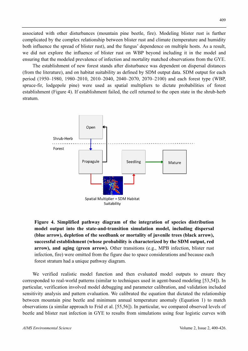
The establishment of new forest stands after disturbance was dependent on dispersal distances (from the literature), and on habitat suitability as defined by SDM output data. SDM output for each period (1950–1980, 1980–2010, 2010–2040, 2040–2070, 2070–2100) and each forest type (WBP, spruce-fir, lodgepole pine) were used as spatial multipliers to dictate probabilities of forest establishment (Figure 4). If establishment failed, the cell returned to the open state in the shrub-herb stratum.

Figure 4. Simplified pathway diagram of the integration of species distribution model output into the state-and-transition simulation model, including dispersal (blue arrow), depletion of the seedbank or mortality of juvenile trees (black arrow), successful establishment (whose probability is characterized by the SDM output, red arrow), and aging (green arrow). Other transitions (e.g., MPB infection, blister rust infection, fire) were omitted from the figure due to space considerations and because each forest stratum had a unique pathway diagram.

We verified realistic model function and then evaluated model outputs to ensure they corresponded to real-world patterns (similar to techniques used in agent-based modeling [53,54]). In particular, verification involved model debugging and parameter calibration, and validation included sensitivity analysis and pattern evaluation. We calibrated the equation that dictated the relationship between mountain pine beetle and minimum annual temperature anomaly (Equation 1) to match observations (a similar approach to Frid et al. [55,56]). In particular, we compared observed levels of beetle and blister rust infection in GYE to results from simulations using four logistic curves with

410


different maxima for the probability of beetle infection. Evaluation of simulation models remains a significant challenge [57,58,59]. Our evaluation

effort was limited by the availability of independent datasets, but we implemented sensitivity analysis and pattern evaluation [60] to check the validity of our model. We sought to reproduce the recent large-scale dynamics of WBP population and disturbance. We compared mountain pine beetle induced WBP mortality using different stratum shift (dead forest stands to open shrub-herb) probabilities to observations from the U.S. Forest Service aerial detection survey. Modeled results were subset by the area flown in each year of the aerial survey.

To test the robustness of our model to parameter uncertainty, we performed sensitivity analysis by running the model for the historical period with different values for parameters that might change substantially with climate or had lower certainty (were unknown or estimated, see Supplementary Material). In particular, we varied the probabilities of alpine colonization by WBP, replacement fire, and spruce-fir replacement of WBP stands by +/−50% [54, 61]. We ran 40 Monte Carlo simulations (iterations or model runs) for each perturbation, and compared the means of our primary outcome variables (WBP population, and mountain pine beetle mortality and infection at year 2010) to those from the original model specification. The sensitivity index [61] was calculated as:

x//

(2)

where p is the value of the independent variable, dp is the value for a change of p, x is the value of the dependent variable, and dx is the corresponding change in x in response to the change in p.

After model verification and validation we ran the STSM using a no climate change scenario and multiple scenarios that included combinations of two GCMs (CNRM-CM5 and HadGEM2-AO) and two RCPs (4.5 and 8.5) to capture the range of change in projected WBP habitat suitability. We compared temporal patterns and values of key outcome variables at 2100 for these four climate scenarios and a no climate change scenario. The no climate change scenario used SDM output from 1950‒1980 and the mean probability of mountain pine beetle infection for the same period.

4. Results

4.1. Verification and validation

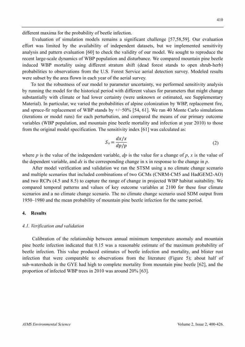
Calibration of the relationship between annual minimum temperature anomaly and mountain pine beetle infection indicated that 0.15 was a reasonable estimate of the maximum probability of beetle infection. This value produced estimates of beetle infection and mortality, and blister rust infection that were comparable to observations from the literature (Figure 5); about half of sub-watersheds in the GYE had high to complete mortality from mountain pine beetle [62], and the proportion of infected WBP trees in 2010 was around 20% [63].

411


Figure 5. Results of model calibration using four different maxima for the probability of mountain pine beetle (MPB) infection (bars) as compared to observations (points). Columns represent the means of 40 Monte Carlo simulations and error bars the standard deviations.

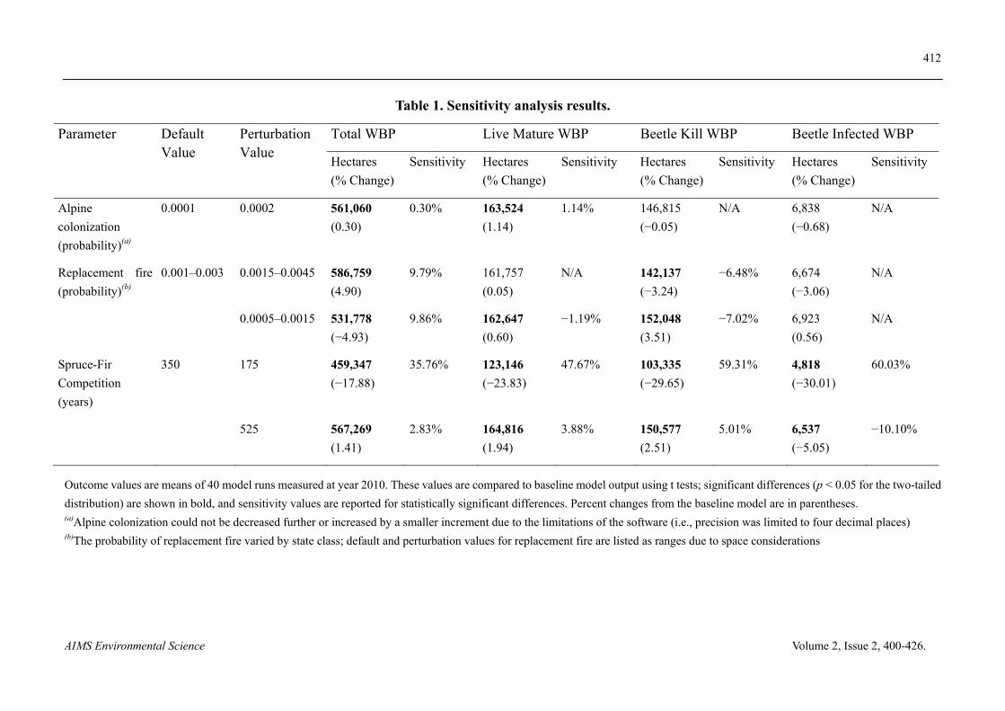
We also tested the sensitivity of key model outputs (total WBP, live mature WBP, beetle kill WBP, and beetle infected WBP) to changes in parameters with less certainty (alpine colonization, replacement fire, and spruce-fir competition) (Table 1). Perturbations of all of the three parameters produced significant differences in one of the three main model outputs. Reducing (by 50%) the time required for spruce-fir forest to replace WBP produced the largest sensitivity index values.

412


Table 1. Sensitivity analysis results.

Parameter Default Value

Perturbation Value

Total WBP Live Mature WBP Beetle Kill WBP Beetle Infected WBP

Hectares

(% Change)

Sensitivity Hectares

(% Change)


(% Change)


(% Change)

Sensitivity

Alpine

colonization

(probability)(a)

0.0001 0.0002 561,060

(0.30)

0.30%

163,524

(1.14)

1.14%

146,815

(−0.05)

N/A

6,838

(−0.68)

N/A

Replacement fire

(probability)(b)

0.001–0.003 0.0015–0.0045 586,759

(4.90)

9.79%

161,757

(0.05)

N/A

142,137

(−3.24)

−6.48%

6,674

(−3.06)

N/A

0.0005–0.0015 531,778

(−4.93)

9.86%

162,647

(0.60)

−1.19%

152,048

(3.51)

−7.02%

6,923

(0.56)

N/A

Spruce-Fir

Competition

(years)

350 175 459,347

(−17.88)

35.76%

123,146

(−23.83)

47.67%

103,335

(−29.65)

59.31%

4,818

(−30.01)

60.03%

525 567,269

(1.41)

2.83%

164,816

(1.94)

3.88%

150,577

(2.51)

5.01%

6,537

(−5.05)

−10.10%

Outcome values are means of 40 model runs measured at year 2010. These values are compared to baseline model output using t tests; significant differences (p < 0.05 for the two-tailed

distribution) are shown in bold, and sensitivity values are reported for statistically significant differences. Percent changes from the baseline model are in parentheses. (a)Alpine colonization could not be decreased further or increased by a smaller increment due to the limitations of the software (i.e., precision was limited to four decimal places) (b)The probability of replacement fire varied by state class; default and perturbation values for replacement fire are listed as ranges due to space considerations

413


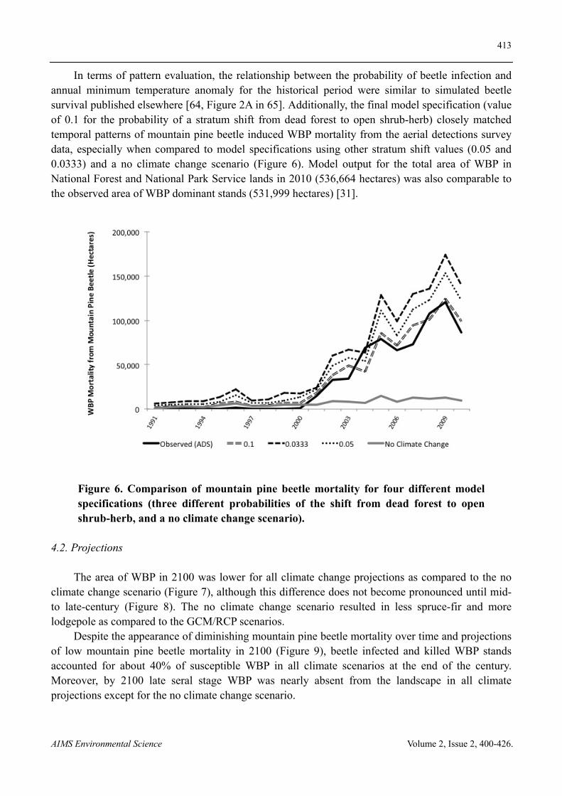
In terms of pattern evaluation, the relationship between the probability of beetle infection and annual minimum temperature anomaly for the historical period were similar to simulated beetle survival published elsewhere [64, Figure 2A in 65]. Additionally, the final model specification (value of 0.1 for the probability of a stratum shift from dead forest to open shrub-herb) closely matched temporal patterns of mountain pine beetle induced WBP mortality from the aerial detections survey data, especially when compared to model specifications using other stratum shift values (0.05 and 0.0333) and a no climate change scenario (Figure 6). Model output for the total area of WBP in National Forest and National Park Service lands in 2010 (536,664 hectares) was also comparable to the observed area of WBP dominant stands (531,999 hectares) [31].

Figure 6. Comparison of mountain pine beetle mortality for four different model specifications (three different probabilities of the shift from dead forest to open shrub-herb, and a no climate change scenario).

4.2. Projections

The area of WBP in 2100 was lower for all climate change projections as compared to the no climate change scenario (Figure 7), although this difference does not become pronounced until mid- to late-century (Figure 8). The no climate change scenario resulted in less spruce-fir and more lodgepole as compared to the GCM/RCP scenarios.

Despite the appearance of diminishing mountain pine beetle mortality over time and projections of low mountain pine beetle mortality in 2100 (Figure 9), beetle infected and killed WBP stands accounted for about 40% of susceptible WBP in all climate scenarios at the end of the century. Moreover, by 2100 late seral stage WBP was nearly absent from the landscape in all climate projections except for the no climate change scenario.

414


Figure 7. Mean areas of three forest types in 2100 under five different climate scenarios. Error bars represent the 95% percentile range for 40 Monte Carlo simulations.

Figure 8. Projected area of WBP forest under five different climate scenarios. Lines represent the means of 40 Monte Carlo simulations and shaded regions represent the 95% percentile range.

415


Figure 9. Projected area of WBP mortality from mountain pine beetle under five different climate scenarios. Lines represent the means of 40 Monte Carlo simulations and shaded regions represent the 95% percentile range.

5. Discussion

Results of the sensitivity analysis suggest that some of the less certain model parameters had a substantial effect on model output. The time for WBP stands to transition to spruce-fir forest had the largest effect. More detailed information on this dynamic would likely improve model reliability. Estimates for seral (as opposed to climax) WBP communities for this parameter range from 100‒200 years [66]. Although the 350-year replacement time used in the model produced relatively conservative estimates of WBP persistence, a more nuanced approach could link spruce-fir competition to other factors (e.g., elevation). It is possible that this and other influential parameters, such as the rate of WBP colonization of the alpine zone and variation in the probability of stand replacing fires with climate, could be estimated based on fire, reforestation, and climatic patterns that have been reconstructed from fossil records [30,67].

Another limitation of this modeling effort was the use of output from SDMs of adult trees as input for seedling establishment. In other words, the spatial multiplier files used in our model represent the probability of the presence of adult trees, but dictated the probability of seedling establishment. However, these probability surfaces were based on 30-year moving averages of climate variables, so, depending on the age of the adult trees, these data may indeed represent the climate conditions during establishment. Moreover, our comparison of the presence and absence locations of mature and seedling WBP suggests that the distribution of seedlings is very similar to that of adults. In sum, without additional data points for the presence and absence of seedlings to parameterize more robust seedling SDMs, and given the overlap in WBP adult and seedling distributions it seems reasonable to have used the available SDM output for seedling establishment within the STSM.

Despite these limitations, the model produced results that closely matched historical point

416


estimates and temporal patterns of WBP and mountain pine beetle activity in the GYE, indicating realistic model function. The counterintuitive finding of less spruce-fir under no climate change is likely the result of mountain pine beetle activity; the no climate change scenario had lower beetle infection probabilities, less beetle mortality, and thus fewer opportunities for spruce-fir to colonize cells vacated by beetle-killed lodgepole and WBP. Future work could incorporate SDM output of historic and projected mountain pine beetle habitat suitability in order to provide more nuanced and spatially explicit infection probabilities.

Output for key WBP variables were comparable across GCMs and RCPs. All scenarios showed a substantial decline in WBP forest, and especially late seral stage forest. The differential effects of climate projections may have been attenuated by similar levels of mountain pine beetle activity across climate scenarios. Across all climate projections, the probability of mountain pine beetle infection reaches a maximum by early- to mid-century.

Overall, this modeling effort integrated a wide range of available information on WBP ecology, reproduced observed patterns of WBP mortality in the GYE, and set the stage for future exploration of WBP management scenarios. The sensitivity analyses and findings also point to the importance of accounting for climate, disturbances, biotic interactions, and habitat suitability together. The approach outlined here for combining the SDMs and STSMs provides a strong foundation for exploring alternative approaches to managing resources under the combined pressures of climate change, insects, disease, and interspecific competition.

6. Conclusion

This research demonstrated the benefits of integrating correlative and stochastic simulation models. In particular, we combined SDM’s ability to produce statistically robust estimates of the relationship between climate and habitat with STSM’s ability to account for disturbances and biotic interactions. The resulting model reproduced observed patterns of WBP in the GYE.

Another important outcome from this research is the identification of data gaps and opportunities for the integration of additional datasets and modeling approaches. Our framework for model validation not only served to corroborate model function, but also identified important research needs, including the ability of WBP to colonize alpine zones, the rate of spruce-fir replacement of WBP across different parts of the landscape, and changes in fire regime. Looking to the historical and paleontological record could help address these shortcomings.

This model and the software platform offer a basis for exploring resource management scenarios such as thinning to protect high value trees from fire, prescribed fires, and the application of pesticides and pheromones to deter mountain pine beetles [31]. Ideally, the specific management scenarios would be carefully developed in conjunction with resource managers. Scenarios could then be implemented in ST-Sim by altering transition probabilities to further explore parameter space and model sensitivity, setting management targets for a given outcome (e.g., area of beetle mortality), or setting limits on expenditures for a given action (e.g., pesticide application). Moreover, these scenarios could be applied to specific management units (e.g., National Forests, National Parks), locations (e.g., < 10 km from roadways), and time periods. The costs of implementing management actions or achieving particular targets could also be tracked through time.

STSMs can integrate a variety of data types and sources to create spatially explicit, flexible, and verifiable representations of ecological dynamics. When paired with SDMs, they offer an especially

417


powerful approach for anticipating the effects of climate change, and ultimately, exploring options for managing species in the face of an uncertain future.

Acknowledgments

We are grateful to Rick Lawrence for sharing data that were used to help initialize the STSM. We also thank Catherine Jarnevich and an anonymous reviewer for their helpful comments on previous drafts of this paper. This research was funded by the U.S. Geological Survey’s North Central Climate Science Center. Any use of trade, product, or firm names is for descriptive purposes only and does not imply endorsement by the U.S. Government.

Conflict of Interest

All authors declare no conflicts of interest in this paper.

418


Supplementary

Appendix S1. Probabilistic transition parameter values, sources, and associated transition constraints.

From Veg.

Type

From Class To Veg.

Type

To Class Transition Type Probability Age

(years)

Source & Notes Other Transition Constraints

All Forest Propagule All Forest Juvenile Establishment From SDM ≥ 1 SDM output (habitat suitability grids)

All forest Dead-Fire Shrub-Herb Open Succession Deterministic ≥ 2 Allows for seed dispersal to open cells after

fire

Alpine Open WBP Propagule Colonization 0.0001 ≥ 1 Estimated/unknown; tested with sensitivity

analysis

Lodgepole Late-Close Spruce-Fir Mature Competition Deterministic 350 LANDFIRE BPS 2110550 [68] Min. time-since-transition (TST)

(establishment) = 350 yr.

Lodgepole Mid-Close Lodgepole Mid-Close Competition/Main

tenance

0.0020 20‒79

Lodgepole MPB Lodgepole Dead-

MPB

Death-MPB Deterministic ≥ 20 Probability of death incorporated into

probability of infection (as in LANDFIRE)

Min. TST (MPB infection) = 2 yr.

Lodgepole Propagule Shrub-Herb Open Establishment

Failure

0.9500 ≥ 1 Probability assumed equal for all forest

types

Min. TST (dispersal) = 11 yr.

(estimated based on MPB stands,

Teste et al. [69])

Lodgepole Mid-Close Lodgepole MPB Infection-MPB 0.0030 20‒79 LANDFIRE BPS 2110550 [68] Annual temporal multipliers vary

this parameter according to

Equation 1; outbreak size

distribution estimated based on

Aukema et al. [52]

Lodgepole Late-Close Lodgepole MPB Infection-MPB 0.0030 80‒350

Lodgepole Late-Close Lodgepole Mid-Close Insect/Disease-

Other

0.0060 80‒350

419


Lodgepole All Lodgepole Dead-Fire Replacement Fire 0.0030 ≥ 1 LANDFIRE BPS 2110550 [68]; tested

with sensitivity analysis

Fire size distribution (MTBS [70])

Lodgepole Dead-MPB Shrub-Herb Open Succession 0.1000 > 20 Based on time for shrub-herb to early forest

(10‒30yrs, Keane et al. [66]); used to track

amount of dead forest

Min. TST (MPB mortality) = 2 yr.

(loss of needles)

Shrub-Herb Open All Forest Propagule Succession 0.2500 ≥ 1 Probability assumed equal for all forest

types

Seed dispersal distances (USFS

[71])

Spruce-Fir Propagule Shrub-Herb Open Establishment

Failure

0.9500 ≥ 1 Min. TST (dispersal) = 3 yr.

(Johnson & Fryer [72])

Spruce-Fir Late-Close Spruce-Fir Late-Open Insect/Disease-

Other

0.0010 ≥ 150 LANDFIRE BPS 2110560 [68]

Spruce-Fir Late-Close Spruce-Fir Late-Open Mixed Fire 0.0050 ≥ 150

Spruce-Fir Early Spruce-Fir Dead-Fire Replacement Fire 0.0020 1‒39 LANDFIRE BPS 2110560 [68]; tested



Spruce-Fir Mid-Close,

-Open

Spruce-Fir Dead-Fire Replacement Fire 0.0020 40‒149

Spruce-Fir Late-Open Spruce-Fir Dead-Fire Replacement Fire 0.0025 ≥ 150

Spruce-Fir Early Spruce-Fir Mid-Open Succession 0.0010 1‒39 LANDFIRE BPS 2110560 [68]

Spruce-Fir Late-Open Spruce-Fir Late-Close Succession 0.0010 ≥ 150

Spruce-Fir Mid-Close Spruce-Fir Mid-Open Wind/Weather/

Stress

0.0010 40‒149

WBP Late-Close Spruce-Fir Mid-Close Competition Deterministic 350 Based on LANDFIRE BPS 2110550 [68];

tested with sensitivity analysis

Min. TST (establishment) = 350

yr.

WBP Mid-Close WBP Mid-Close Competition/

Maintenance

0.0020 50‒129 LANDFIRE BPS 2110460 [68]

WBP Early WBP Early Competition/

Maintenance

0.0050 1‒49

420


WBP MPB, Rust

& MPB

WBP Dead-

MPB

Death-MPB Deterministic ≥ 51 Probability of death combined with

probability of infection (as in LANDFIRE)

Min. TST (MPB infection) = 2 yr.

WBP Rust-Early WBP Dead-Rust Death-Rust 0.5213 ≥ 1 Keane et al. [66] TST (rust infection) = 10‒30yrs

(Hatala and Crabtree [73])

WBP Rust-Mature WBP Dead-Rust Death-Rust 0.5213 ≥ 50

WBP Propagule Shrub-Herb Open Establishment

Failure

0.9500 ≥ 1 Probability assumed equal for all forest

types

Min. TST (dispersal) = 4 yr.

(USFS [71], Keane et al. [66])

WBP Mid-Close WBP MPB Infection-MPB 0.0030 50‒129 LANDFIRE BPS 2110460 [68] Annual temporal multipliers vary

this parameter according to

Equation 1; outbreak size

distribution estimated based on

Aukema et al. [52]

WBP Late-Close WBP MPB Infection-MPB 0.0030 130‒350

WBP Mid-Open WBP MPB Infection-MPB 0.0020 50‒129

WBP Late-Open WBP MPB Infection-MPB 0.0020 ≥ 130

WBP Mid-Open,

-Close

WBP Rust-

Mature

Infection-Rust 0.0067 50‒129 Logan et al. [65]; also similar to Keane et

al. [66]

Initiated in 1970; outbreak size

distribution (estimated)

WBP Late-Open,

-Close

WBP Rust-

LANDFI

RE Mature

Infection-Rust 0.0067 ≥ 130

WBP Early WBP Rust-Early Infection-Rust 0.0184 1‒49 Keane et al. [66]

WBP Late-Close WBP Late-Open Insect/Disease-

Other

0.0020 130‒350 LANDFIRE BPS 2110460 [68]

WBP Mid-Close WBP Mid-Open Insect/Disease-

Other

0.0030 50‒129

WBP Late-Close WBP Late-Open Mixed Fire 0.0020 130‒350

WBP Mid-Open WBP Mid-Open Mixed Fire 0.0070 50‒129

WBP Late-Open WBP Late-Open Mixed Fire 0.0070 ≥ 130

421


WBP Mid-Close WBP Mid-Open Mixed Fire 0.0040 50‒129

WBP Dead-MPB WBP Dead-Fire Replacement Fire 0.0025 ≥ 52 Estimated based on fire probabilities from

BPS 2110460 (mixed evidence for

influence of beetle/rust kill on fire); tested



WBP Dead-Rust WBP Dead-Fire Replacement Fire 0.0025 ≥ 2 Fire size distribution (MTBS [70])

WBP Rust-Early WBP Dead-Fire Replacement Fire 0.0025 1‒49

WBP Rust-Mature WBP Dead-Fire Replacement Fire 0.0025 ≥ 50

WBP MPB, Rust

& MPB

WBP Dead-Fire Replacement Fire 0.0025 ≥ 51

WBP Early WBP Dead-Fire Replacement Fire 0.0010 1‒49 LANDFIRE BPS 2110460 [68]; tested


WBP Mid-Close WBP Dead-Fire Replacement Fire 0.0020 50‒129

WBP Late-Close WBP Dead-Fire Replacement Fire 0.0020 130‒350

WBP Mid-Open WBP Dead-Fire Replacement Fire 0.0030 50‒129

WBP Late-Open WBP Dead-Fire Replacement Fire 0.0030 ≥ 130

WBP Early WBP Mid-Open Succession 0.0100 1‒49 LANDFIRE BPS 2110460 [68]

WBP Mid-Open WBP Mid-Close Succession 0.0500 50‒129

WBP Late-Open WBP Late-Close Succession 0.0500 ≥ 130

WBP Dead-MPB Shrub-Herb Open Succession 0.1000 ≥ 52 Based on time to transition from

shrub-herb to early forest (10‒30yrs,

Keane et al. [66]) in order to track amount

of dead forest

Min. TST (MPB mortality) = 2 yr.

(loss of needles)

WBP Dead-Rust Shrub-Herb Open Succession 0.1000 ≥ 2

422


References

1. Miller BW, Morisette JT (2014) Integrating research tools to support resource management under climate change. Ecol Soc 19: 41.

2. Guisan A, Thuiller W (2005) Predicting species distribution: Offering more than simple habitat models. Ecol Lett 8: 993-1009.

3. Sinclair SJ, White MD, Newell GR (2010) How useful are species distribution models for managing biodiversity under future climates? Ecol Soc 15: 8.

4. Daniel CJ, Frid L (2012) Predicting landscape vegetation dynamics using state-and-transition simulation models, In: Kerns BK, Shlisky AJ, Daniel CJ, technical editors, Proc First Landscape State-and-Transition Sim Model Conf, June 14–16, 2011, Portland, OR, Gen Tech Rep PNW-GTR-869, Portland, OR: U.S. Department of Agriculture, Forest Service, Pacific Northwest Research Station, 5-22.

5. Franklin J (2009) Mapping species distributions: Spatial inference and prediction. Cambridge, UK: Cambridge University Press.

6. Franklin J (2013) Species distribution models in conservation biogeography: Developments and challenges. Div Distr 19: 1217-1223.

7. Dobrowski SZ, Thorne JH, Greenberg JA, et al. (2011) Modeling plant ranges over 75 years of climate change in California, USA: Temporal transferability and species traits. Ecol Monogr 81: 241-257.

8. Bell DM, Bradford JB, Lauenroth WK (2014) Early indicators of change: Divergent climate envelopes between tree life stages imply range shifts in the western United States. Global Ecol Biogeog 23: 168-180.

9. Stephenson NL (1998) Actual evapotranspiration and deficit: Biologically meaningful correlates of vegetation distribution across spatial scales. J Biogeogr 25: 855-870.

10. Benito-Garzón M, Ha-Duong M, Frascaria-Lacoste N, et al. (2013) Habitat restoration and climate change: Dealing with climate variability, incomplete data, and management decisions with tree translocations. Restor Ecol 21: 530-536.

11. Schwartz MW (2012) Using niche models with climate projections to inform conservation management decisions. Biol Cons 155: 149-156.

12. Iverson LR, Prasad AM, Matthews SN, et al. (2011) Lessons learned while integrating habitat, dispersal, disturbance, and life-history traits into species habitat models under climate change. Ecosystems 14: 1005-1020.

13. Westoby M, Walker B, Noy-Meir I (1989) Opportunistic management for rangelands not at equilibrium. J Range Manage 42: 266-274.

14. Bestelmeyer BT, Brown JR, Havstad KM, et al. (2003) Development and use of state-and-transition models for rangelands. J Range Manage 56: 114-126.

15. Stringham TK, Krueger WC, Shaver PL (2001) States, transitions, and thresholds: Further refinement for rangeland applications. Special Report Number 1024, Oregon State University Agricultural Experiment Station: 1-15.

16. Parker DC, Manson SM, Janssen MA, et al. (2003) Multi-agent systems for the simulation of land-use and land-cover change: A review. Ann Assoc American Geogr 93: 314-337.

423


17. Li H, Reynolds JF (1997) Modeling effects of spatial pattern, drought, and grazing on rates of rangeland degradation: A combined Markov and cellular automaton approach, In: Quattrochi DA, Goodchild MF, editors, Scale in Remote Sensing and GIS, Boca Raton, FL: Lewis Publishers, 211-230.

18. Balzter H, Braun PW, Köhler W (1998) Cellular automata models for vegetation dynamics. Ecol Model 107: 113-125.

19. Bestelmeyer BT, Goolsby DP, Archer SR (2011) Spatial perspectives in state-and-transition models: A missing link to land management? J Appl Ecol 48: 746-757.

20. Forbis TA, Provencher L, Frid L, et al. (2006) Great Basin land management planning using ecological modeling. Environ Manage 38: 62-83.

21. Provencher L, Forbis TA, Frid L, et al. (2007) Comparing alternative management strategies of fire, grazing, and weed control using spatial modeling. Ecol Model 209: 249-263.

22. Frid L, Wilmshurst JF (2009) Decision analysis to evaluate control strategies for Crested Wheatgrass (Agropyron cristatum) in Grasslands National Park of Canada. Invasive Plant Sci Manage 2: 324-336.

23. Costanza JK, Hulcr J, Koch FH, et al. (2012) Simulating the effects of the southern pine beetle on regional dynamics 60 years into the future. Ecol Model 244: 93-103.

24. Keane RE, Holsinger LM, Parsons RA, et al. (2008) Climate change effects on historical range and variability of two large landscapes in western Montana, USA. Forest Ecol Manage 254: 375-389.

25. Strand EK, Vierling LA, Bunting SC, et al. (2009) Quantifying successional rates in western aspen woodlands: Current conditions, future predictions. Forest Ecol Manage 257: 1705-1715.

26. Halofsky JE, Hemstrom MA, Conklin DR, et al. (2013) Assessing potential climate change effects on vegetation using a linked model approach. Ecol Model 266: 131-143.

27. Hemstrom MA, Halofsky JE, Conklin DR, et al. (2014) Developing climate-informed state-and-transition models, In: Halofsky JE, Creutzburg MK, Hemstrom MA, editors, Integrating Social, Economic, and Ecological Values Across Large Landscapes, Gen Tech Rep PNW-GTR-896, Portland, OR: U.S. Department of Agriculture, Forest Service, Pacific Northwest Research Station, 175-202.

28. Yospin GI, Bridgham SD, Neilson RP, et al. (2014) A new model to simulate climate change impacts on forest succession for local land management. Ecol Appl 25:226-242.

29. Chang T, Hansen AJ, Piekielek N (2014) Patterns and variability of projected bioclimatic habitat for Pinus albicaulis in the Greater Yellowstone Area. PLoS ONE 9: e111669.

30. Whitlock C (1993) Postglacial vegetation and climate of Grand Teton and southern Yellowstone National Parks. Ecol Monogr 63: 173-198.

31. Greater Yellowstone Coordinating Committee Whitebark Pine Subcommittee (2011) Whitebark Pine Strategy for the Greater Yellowstone Area. US Dept of Agriculture, Forest Service, Forest Health Protection, and Grand Teton National Park.

32. Gibson K, Skov K, Kegley S, et al. (2008) Mountain pine beetle impacts in high-elevation five-needle pines: current trends and challenges. US Department of Agriculture, Forest Service, Forest Health Protection.

33. Larson ER, Kipfmueller KF (2012) Ecological disaster or the limits of observation? Reconciling modern declines with the long-term dynamics of whitebark pine communities. Geogr Compass 6: 189-214.

424


34. Romme WH, Turner MG (1991) Implications of global climate change for biogeographic patterns in the Greater Yellowstone Ecosystem. Conserv Biol 5: 373-386.

35. Bartlein PJ, Whitlock C, Shafer SL (1997) Future climate in the Yellowstone national park region and its potential impact on vegetation. Conserv Biol 11: 782-792.

36. Schrag AM, Bunn AG, Graumlich LJ (2008) Influence of bioclimatic variables on tree‐line conifer distribution in the Greater Yellowstone Ecosystem: Implications for species of conservation concern. J Biogeogr 35(4): 698-710.

37. U.S. Fish and Wildlife Service (2011) Whitebark pine to be designated a candidate for endangered species protection. Available from: http://www.fws.gov/Wyominges/Pages/Species/Findings/2011_WBP.html

38. Freire J (2012) Making computations and publications reproducible with VisTrails. Comput Sci Eng 14: 18-25.

39. Morisette JT, Jarnevich CS, Holcombe TR, et al. (2013) VisTrails SAHM: Visualization and workflow management for species habitat modeling. Ecography 36: 129-135.

40. Lockman IB, DeNitto GA, Courter A, et al. (2007) WLIS: The whitebarklimber pine information system and what it can do for you. In: Proceedings of the Conference Whitebark Pine: A Pacific Coast Perspective. Ashland, OR: US Department of Agriculture, Forest Service, Pacific Northwest Region, 146-147.

41. Greater Yellowstone Whitebark Pine Monitoring Working Group (2011) Interagency Whitebark Pine Monitoring Protocol for the Greater Yellowstone Ecosystem, Version 1.1. Greater Yellowstone Coordinating Committee, Bozeman, MT. Available from: http://fedgycc.org/documents/GYE.WBP.MonitoringProtocol.V1.1June2011.pdf

42. Smith WB (2002) FIA: Forest inventory and analysis: a national inventory and monitoring program. Environ Pollut 116: S233-S242.

43. Gibson J, Moisen G, Frescino T, et al. (2014) Using publicly available forest inventory data in climate-based models of tree species distribution: Examining effects of true versus altered location coordinates. Ecosystems 17: 43-53.

44. Drake BG, Gonzàlez-Meler MA, Long SP (1997) More efficient plants: A consequence of rising atmospheric CO2? Annu Rev Plant Biol 48: 609-639.

45. Lobo JM, Jiménez-Valverde A, Real R (2008) AUC: A misleading measure of the performance of predictive distribution models. Global Ecol Biogeogr 17: 145-151.

46. Voldoire A, Sanchez-Gomez E, Salas y Mélia, et al. (2013) The CNRM-CM5. 1 global climate model: Description and basic evaluation. Clim Dynam 40: 2091-2121.

47. Martin GM, Bellouin N, Collins WJ, et al. (2011) The HadGEM2 family of met office unified model climate configurations. Geosci Model Dev 4: 723-757.

48. Deser C, Phillips AS, Alexander MA, et al. (2014) Projecting North American climate over the next 50 years: Uncertainty due to internal variability. J Climate 27: 2271-2296.

49. Apex Resource Management Solutions (2014) ST-Sim state-and-transition simulation model software. Available from: www.apexrms.com/stsm

50. Rollins MG (2009) LANDFIRE: A nationally consistent vegetation, wildland fire, and fuel assessment. Int J Wildland Fire 18: 235-249.

51. Landenburger L, Lawrence RL, Podruzny S, et al. (2008) Mapping regional distribution of a single tree species: Whitebark Pine in the Greater Yellowstone Ecosystem. Sensors 8: 4983-4994.

425


52. Aukema BH, Carroll AL, Zhu J, et al. (2006) Landscape level analysis of mountain pine beetle in British Columbia, Canada: Spatiotemporal development and spatial synchrony within the present outbreak. Ecography 29: 427-441.

53. An L, Linderman M, Qi J, et al. (2005) Exploring complexity in a human-environment system: An agent-based spatial model for multidisciplinary and multiscale integration. Ann Assoc American Geogr 95, 54-79.

54. Miller BW, Breckheimer I, McCleary AL, et al. (2010) Using stylized agent-based models for population-environment research: a case study from the Galápagos Islands. Popul Environ 31: 401-426.

55. Frid L, Hanna D, Korb N, et al. (2013) Evaluating alternative weed management strategies for three Montana landscapes. Invasive Plant Sci Manage 6: 48-59.

56. Frid L, Holcombe T, Morisette JT, et al. (2013) Using state-and-transition modeling to account for imperfect detection in invasive species management. Invasive Plant Sci Manage 6: 36-47.

57. Windrum P, Fagiolo G, Moneta A (2007) Empirical validation of agent-based models: Alternatives and prospects. J Artif Soc Soc Simulat 10: 8.

58. Oreskes N, Shrader-Frechette K, Belitz K (1994) Verification, validation, and confirmation of numerical models in the earth sciences. Science 263: 641-646.

59. Oreskes N (1998) Evaluation (not validation) of quantitative models. Environmental Health Perspectives 106: 1453-1460.

60. Grimm V, Revilla E, Berger U, et al. (2005) Pattern-oriented modeling of agent-based complex systems: Lessons from ecology. Science 310: 987-991.

61. Jørgensen SE (1986) Fundamentals of Ecological Modelling. Amsterdam: Elsevier. 62. Macfarlane WW, Logan JA, Kern WR (2009) Using the landscape assessment system (LAS) to

assess mountain pine beetle-caused mortality of whitebark pine, Greater Yellowstone Ecosystem, 2009. Project report prepared for the Greater Yellowstone Coordinating Committee, Whitebark Pine Subcommittee, Jackson, WY.

63. Shanahan E, Irvine KM, Roberts D, et al. (2014) Status of whitebark pine in the Greater Yellowstone Ecosystem: A step-trend analysis comparing 2004-2007 to 2008- 2011. Natural Resource Technical Report NPS/GRYN/NRTR—2014/917. Fort Collins, CO: National Park Service.

64. Régnière J, Bentz BJ (2007) Modeling cold tolerance in the mountain pine beetle, Dendroctonus pondersoae. J Insect Physiol 53: 559-572.

65. Logan JA, Macfarlane WW, Wilcox L (2010) Whitebark pine vulnerability to climate-driven mountain pine beetle disturbance in the Greater Yellowstone Ecosystem. Ecol Appl 20: 895-902.

66. Keane RE (2001) Successional dynamics: Modeling an anthropogenic threat, In: Tomback DF, Arno SF, Keane RE, editors, Whitebark Pine Communities: Ecology and Restoration. Washington, DC: Island Press, 159-192.

67. Whitlock C, Millspaugh, SH (2001) A paleoecologic perspective on past plant invasions in Yellowstone. West N Am Naturalist 61: 316-327.

68. LANDFIRE (Landscape Fire and Resource Management Planning Tools Project) dataset. Available online at www.landfire.gov.

69. Teste FP, Lieffers VJ, Landhausser SM (2011) Viability of forest floor and canopy seed banks in Pinus contorta var. latifoia (Pinaceas) forests after a mountain pine beetle outbreak. American Journal of Botany 98: 630-637.

426


70. MTBS (Monitoring Trends in Burn Severity) dataset. Available from: at www.mtbs.gov. 71. USFS (United States Forest Service), Species life history information. Available from:

www.fs.fed.us. 72. Johnson EA, Fryer GI (1996) Why Engelmann spruce does not have a persistent seed bank.

Canadian Journal of Forest Research, 26: 872-878 73. Hatala JA, Crabtree, RL (2009) Modelling the spread of blister rust in the Greater Yellowstone

Ecosystem. Nutcracker Notes, Whitebark Pine Ecosystem Foundation 16: 17-18.

© 2015, Brian W. Miller, et al., licensee AIMS Press. This is an open access article distributed under the terms of the Creative Commons Attribution License (http://creativecommons.org/licenses/by/4.0)

combining state-and-transition simulations and species distribution

Documents