combinatorics mt454 / mt5454 - semantic scholar · combinatorial arguments may be found lurking in...
TRANSCRIPT

COMBINATORICS MT454 / MT5454
MARK WILDON
These notes are intended to give the logical structure of the course;proofs and further remarks will be given in lectures. Further install-ments will be issued as they are ready. All handouts and problem sheetswill be put on Moodle.
I would very much appreciate being told of any corrections or possibleimprovements to these notes.
You are warmly encouraged to ask questions in lectures, and to talk tome after lectures and in my office hours. I am also happy to answerquestions about the lectures or problem sheets by email. My email ad-dress is [email protected].
Lectures: Tuesday 11am in C201, Wednesday 12 noon in ABLT3 andThursday 3pm in C336.
Office hours in McCrea 240: Monday 4pm, Wednesday 10am and Fri-day 4pm.
Date: First term 2013/14.
2
1. INTRODUCTION
Combinatorial arguments may be found lurking in all branches ofmathematics. Many people first become interested in mathematics bya combinatorial problem. But, strangely enough, at first many mathe-maticians tended to sneer at combinatorics. Thus one finds:
“Combinatorics is the slums of topology.”J. H. C. Whitehead (early 1900s, attr.)
Fortunately attitudes have changed, and the importance of combina-torial arguments is now widely recognised:
“The older I get, the more I believe that at the bottom of mostdeep mathematical problems there is a combinatorial problem.”
I. M. Gelfand (1990)
Combinatorics is a very broad subject. It will often be useful to provethe same result in different ways, in order to see different combinato-rial techniques at work. There is no shortage of interesting and easilyunderstood motivating problems.
Overview. This course will give a straightforward introduction to fourrelated areas of combinatorics. Each is the subject of current research,and taken together, they give a good idea of what the subject is about.
(A) Enumeration: Binomial coefficients and their properties. Princi-ple of Inclusion and Exclusion and applications. Rook polyno-mials.
(B) Generating Functions: Ordinary generating functions and re-currence relations. Partitions and compositions. Catalan Num-bers. Derangements.
(C) Ramsey Theory: “Complete disorder is impossible”. Pigeon-hole Principle. Graph colouring.
(D) Probabilistic Methods: Linearity of expectation. First momentmethod. Applications to counting permutations. Lovasz LocalLemma.
Recommended Reading.
[1] A First Course in Combinatorial Mathematics. Ian Anderson, OUP1989, second edition.
[2] Discrete Mathematics. N. L. Biggs, OUP 1989, second edition.[3] Combinatorics: Topics, Techniques, Algorithms. Peter J. Cameron,
CUP 1994.[4] Concrete Mathematics. Ron Graham, Donald Knuth and Oren
Patashnik, Addison-Wesley 1994.

3
[5] Invitation to Discrete Mathematics. Jiri Matousek and JaroslavNesetril, OUP 2009, second edition.
[6] Probability and Computing: Randomized Algorithms and Probabilis-tic Analysis. Michael Mitzenmacher and Eli Upfal, CUP 2005.
[7] generatingfunctionology. Herbert S. Wilf, A K Peters 1994, secondedition. Available from http://www.math.upenn.edu/~wilf/
DownldGF.html.
In parallel with the first few weeks of lectures, you will be asked todo some reading from generatingfunctionology: the problem sheets willmake clear what is expected.
Prerequisites.• Permutations and their decomposition into disjoint cycles. (Re-
quired for derangements and for some applications in Part D.)• Basic definitions of graph theory: vertices, edges and complete
graphs. (Required for Part C on Ramsey Theory.)• Basic knowledge of discrete probability. This will be reviewed
in lectures when we get to part D of the course. A handout withall the background results needed from probability theory willbe issued later in term.
Problem sheets and exercises. There will be weekly problem sheets;the first will be due in on Tuesday 15th October. Exercises set in thesenotes are intended to be simple tests that you are following the material.Some will be done in lectures. Doing the others will help you to reviewthe lectures.
Moodle. Provided you have an RHUL account, you have access to theMoodle page for this course: moodle.rhul.ac.uk/course/view.php?id=371. If you are registered for the course then it will appear under‘My Courses’ on Moodle.
Note on optional questions. Optional questions on problem sheets areincluded for interest and to give extra practice. Harder optional ques-tions are marked (?). If you can do the compulsory questions andknow the bookwork, i.e. the definitions, main theorems, and theirproofs, as set out in the handouts and lectures, you should do verywell in the exam.
4
2. BASIC COUNTING PRINCIPLES AND DERANGEMENTS
In the first two lectures we will see the Derangements Problem andone way to solve it by ad-hoc methods. Later in the course we will de-velop techniques that can be used to solve this problem more easily.
Definition 2.1. A permutation of a set X is a bijective function
σ : X → X.
A fixed point of a permutation σ of X is an element x ∈ X such thatσ(x) = x. A permutation is a derangement if it has no fixed points.
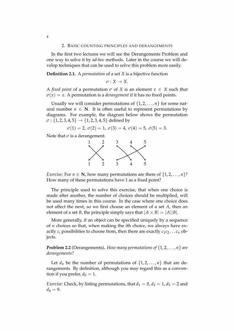
Usually we will consider permutations of 1, 2, . . . , n for some nat-ural number n ∈ N. It is often useful to represent permutations bydiagrams. For example, the diagram below shows the permutationσ : 1, 2, 3, 4, 5 → 1, 2, 3, 4, 5 defined by
σ(1) = 2, σ(2) = 1, σ(3) = 4, σ(4) = 5, σ(5) = 3.
Note that σ is a derangement.1 2 3 4 5
1 2 3 4 5
Exercise: For n ∈ N, how many permutations are there of 1, 2, . . . , n?How many of these permutations have 1 as a fixed point?
The principle used to solve this exercise, that when one choice ismade after another, the number of choices should be multiplied, willbe used many times in this course. In the case where one choice doesnot affect the next, so we first choose an element of a set A, then anelement of a set B, the principle simply says that |A× B| = |A||B|.
More generally, if an object can be specified uniquely by a sequenceof n choices so that, when making the ith choice, we always have ex-actly ci possibilities to choose from, then there are exactly c1c2 . . . cn ob-jects.
Problem 2.2 (Derangements). How many permutations of 1, 2, . . . , n arederangements?
Let dn be the number of permutations of 1, 2, . . . , n that are de-rangements. By definition, although you may regard this as a conven-tion if you prefer, d0 = 1.
Exercise: Check, by listing permutations, that d1 = 0, d2 = 1, d3 = 2 andd4 = 9.

5
Exercise: Suppose we try to construct a derangement of 1, 2, 3, 4, 5such that σ(1) = 2. Show that there are two derangements such thatσ(1) = 2, σ(2) = 1, and three derangements such that σ(1) = 2, σ(2) =3. How many choices are there for σ(3) in each case?
The previous exercise shows that we can’t hope to solve the derange-ments problem just by multiplying numbers of choices. Instead weshall find a recurrence for the numbers dn.
Lemma 2.3. If n ≥ 2 then the number of derangements σ of 1, 2, . . . , nsuch that σ(1) = 2 is dn−2 + dn−1.
Notice the use of another basic counting principle in Lemma 2.3: ifwe can partition the objects we are counting into two disjoint sets Aand B, then the total number of objects is |A|+ |B|.
Theorem 2.4. If n ≥ 2 then dn = (n− 1)(dn−2 + dn−1).
Using this recurrence relation it is easy to find values of dn for muchlarger n. Whenever one meets a new combinatorial sequence it is agood idea to look it up in N. J. A. Sloane’s Online Encyclopedia of In-teger Sequences: see www.research.att.com/~njas/sequences/. Youwill usually find it in there, along with references and often other com-binatorial interpretations.
Corollary 2.5. For all n ∈ N0,
dn = n!(
1− 11!
+12!− 1
3!+ · · ·+ (−1)n
n!
).
Exercise: Check directly that the right-hand side is an integer.
A more systematic way to derive Corollary 2.5 from Theorem 2.4 willbe seen in Part B of the course. Question 9 on Sheet 1 gives an alterna-tive proof that does not require knowing the answer in advance.
The proof of Corollary 2.5 and Question 9 show that it is helpful toconsider the probability dn/n! that a permutation of 1, 2, . . . , n, cho-sen uniformly at random, is a derangement. Here ‘uniformly at ran-dom’ means that each of the n! permutations of 1, 2, . . . , n is equallylikely to be chosen.
Theorem 2.6. Two probabilistic results on derangements.(i) The probability that a permutation of 1, 2, . . . , n, chosen uniformly at
random, is a derangement tends to 1/e as n→ ∞.(ii) The average number of fixed points of a permutation of 1, 2, . . . , n
is 1.
We shall prove more results like this in Part D of the course.
6
Part A: Enumeration
3. BINOMIAL COEFFICIENTS AND COUNTING PROBLEMS
The following notation is probably already familiar to you.
Notation 3.1. If Y is a set of size k then we say that Y is a k-set, and write|Y| = k. To emphasise that Y is a subset of some other set X then wemay say that Y is a k-subset of X.
We shall define binomial coefficients combinatorially.
Definition 3.2. Let n, k ∈ N0. Let X = 1, 2, . . . , n. The binomial coeffi-cient (n
k) is the number of k-subsets of X.
By this definition, if k 6∈ N0 then (nk) = 0. Similarly if k > n then
(nk) = 0. It should be clear that we could replace X with any other set of
size n and we would define the same numbers (nk).
We should check that the combinatorial definition agrees with theusual definition.
Lemma 3.3. If n, k ∈ N0 and k ≤ n then(
nk
)=
n(n− 1) . . . (n− k + 1)k!
=n!
k!(n− k)!.
The double-counting technique used to prove Lemma 3.3 is often use-ful in combinatorial problems.
Many of the basic properties of binomial coefficients can be givencombinatorial proofs involving explicit bijections. We say that suchproofs are bijective.
Lemma 3.4. If n, k ∈ N0 then(
nk
)=
(n
n− k
).
Lemma 3.5 (Fundamental Recurrence). If n, k ∈ N then(
nk
)=
(n− 1k− 1
)+
(n− 1
k
).
reasoning with subsets, do (n − r)(nr) = (r + 1)( n
r+1) as example.Note r(n
r) = n(n−1r−1) is on Sheet 1. Binomial coefficients are so-named
because of the famous binomial theorem. (A binomial is a product ofthe form xrys.)

7
Theorem 3.6 (Binomial Theorem). Let x, y ∈ C. If n ∈ N0 then
(x + y)n =n
∑k=0
(nk
)xkyn−k.
Exercise: give inductive or algebraic proofs of the previous three results.
Exercise: in New York, how many ways can one start at a junction andwalk to another junction 4 blocks away to the east and 3 blocks away tothe north?
We can now answer a basic combinatorial question: How many waysare there to put k balls into n numbered urns? The answer depends onwhether the balls are distinguishable. We may consider urns of unlim-ited capacity, or urns that can only contain one ball.
Numbered balls Indistinguishable balls
≤ 1 ball per urn
unlimited capacity
Three of the entries can be found fairly easily. The entry in the bottom-right can be found in many different ways: two will be demonstratedin this lecture.
Theorem 3.7. Let n ∈ N and let k ∈ N0. The number of ways to place kindistinguishable balls into n numbered urns of unlimited capacity is (n+k−1
k ).
The following reinterpretation of Theorem 3.7 can be useful.
Corollary 3.8. Let n ∈ N and let k ∈ N0. The number of n-tuples [corrected14th October from k-tuples] (t1, . . . , tn) such that t1, t2, . . . , tn ∈ N0 and
t1 + t2 + · · ·+ tn = k
is (n+k−1k ).
4. FURTHER BINOMIAL IDENTITIES
This is a vast subject and we shall only cover a few aspects. Particu-larly recommended for further reading is Chapter 5 of Concrete Mathe-matics, [4] in the list on page 2.

8
Arguments with subsets. The two identities below are among the mostuseful in practice.
Lemma 4.1 (Subset of a subset). If k, r, n ∈ N0 and k ≤ r ≤ n then(
nr
)(rk
)=
(nk
)(n− kr− k
).
Lemma 4.2 (Vandermonde’s convolution). If a, b ∈ N0 and m ∈ N0 thenm
∑k=0
(ak
)(b
m− k
)=
(a + b
m
).
Corollaries of the Binomial Theorem. The following results can be obtainedby making a strategic choice of x and y in the Binomial Theorem.
Corollary 4.3. If n ∈ N then(
n0
)+
(n1
)+
(n2
)+ · · ·+
(n
n− 1
)+
(nn
)= 2n,
(n0
)−(
n1
)+
(n2
)− · · ·+ (−1)n−1
(n
n− 1
)+ (−1)n
(nn
)= 0.
Corollary 4.4. For all n ∈ N there are equally many subsets of 1, 2, . . . , nof even size as there are of odd size.
Corollary 4.5. If n ∈ N0 and b ∈ N then(
n0
)bn +
(n1
)bn−1 + · · ·+
(n
n− 1
)b +
(nn
)= (1 + b)n.
There is a nice bijective proof of Corollary 4.5; it will appear as aquestion with hints on Sheet 2.
Some identities visible in Pascal’s Triangle. There are a number of niceidentities that express row, column or diagonal sums in Pascal’s Tri-angle.
Lemma 4.6 (Alternating row sums). If n ∈ N, r ∈ N0 and r ≤ n thenr
∑k=0
(−1)k(
nk
)= (−1)r
(n− 1
r
).
Perhaps surprisingly, there is no simple formula for the unsigned rowsums ∑r
k=0 (nk).

9
Lemma 4.7 (Diagonal sums, a.k.a. parallel summation). If n ∈ N, r ∈N0 then
r
∑k=0
(n + k
k
)=
(n + r + 1
r
).
For the column sums on Pascal’s Triangle, see Sheet 1, Question 3.For the other diagonal sum, see Sheet 1, Question 7.
5. PRINCIPLE OF INCLUSION AND EXCLUSION
The Principle of Inclusion and Exclusion (PIE) is way to find the sizeof a union of a finite collection of subsets of a finite universe set X. Theuniverse set we take will depend on the problem we are solving. If A isa subset of X, we denote by A the complement of A in X; i.e.,
A = X\A = x ∈ X : x 6∈ A.We start with the two smallest non-trivial examples of the Principle
of Inclusion and Exclusion.
Example 5.1. If A, B, C are subsets of a finite set X then
|A ∪ B| = |A|+ |B| − |A ∩ B||A ∪ B| = |X| − |A| − |B|+ |A ∩ B|
and
|A ∪ B ∪ C| = |A|+ |B|+ |C|− |A ∩ B| − |B ∩ C| − |C ∩ A|+ |A ∩ B ∩ C|
|A ∪ B ∪ C| = |X| − |A| − |B| − |C|+ |A ∩ B|+ |B ∩ C|+ |C ∩ A| − |A ∩ B ∩ C|
Example 5.2. The n-th (centred) hexagonal number is the number ofdots in the n-th digure below. The formula for |A ∪ B ∪ C| gives a niceway a formula for these numbers.
8
5. Principle of Inclusion and Exclusion
The Principle of Inclusion and Exclusion (PIE) is an elementary wayto find the sizes of unions or intersections of finite sets.
If A is a subset of a universe set X, we denote by A the complementof A in X; i.e.,
A = x ∈ X : x ∈ A.We start with the two smallest non-trivial examples of the principle.
Example 5.1. If A, B, C are subsets of a set X then |A ∪B| = |A| +|B|− |A ∩B| and so
A ∪B = |X|− |A|− |B| + |A ∩B|.
Similarly, |A∪B ∪C| = |A|+ |B|+ |C|− |A∩B|− |B ∩C|− |C ∩A|+|A ∩B ∩ C|, so
A ∪B ∪ C = |X|− |A|− |B|− |C|
+|A ∩B| + |B ∩ C| + |C ∩ A|− |A ∩B ∩ C|.
Example 5.2. The formula for |A ∪ B ∪ C| gives one of the easiestways to find the hexagonal numbers.
, , . . .
In the general setting we have a set X and subsets A1, A2, . . . , An
of X. Let I ⊆ 1, 2, . . . , n be a non-empty index set. We define
AI =
i∈I
Ai.
Thus AI is the set of elements of X which belong to all of the sets Ai
for i ∈ I. By convention we set
A∅ = X.
Theorem 5.3 (Principle of Inclusion Exclusion). If A1, A2, . . . , An aresubsets of a finite set X then
A1 ∪ A2 ∪ · · · ∪ An
=
I⊆1,2,...,n(−1)|I| |AI |.
, . . .
It is easier to find the sizes of the intersections of the three rhombi mak-ing up each hexagon than it is to find the sizes of their unions. When-ever intersections are easier to think about than unions, the PIE is likelyto work well.
10
In the general setting we have a finite universe set X and subsetsA1, A2, . . . , An ⊆ X. For each non-empty subset I ⊆ 1, 2, . . . , n wedefine
AI =⋂
i∈IAi.
Thus AI is the set of elements which belong to all the sets Ai for i ∈ I.For example, if i, j ∈ 1, 2, . . . , n then Ai = Ai and Ai,j = Ai ∩ Aj.By convention we set
A∅ = X.
Theorem 5.3 (Principle of Inclusion and Exclusion). If A1, A2, . . . , An aresubsets of a finite set X then
|A1 ∪ A2 ∪ · · · ∪ An| = ∑I⊆1,2,...,n
(−1)|I||AI |.
Exercise: Check that Theorem 5.3 holds when n = 1 and check that itagrees with Example 5.1 when n = 2 and n = 3.
Exercise: Deduce from Theorem 5.3 that
|A1 ∪ A2 ∪ · · · ∪ An| = ∑I⊆1,2,...,n
I 6=∅
(−1)|I|−1|AI |.
APPLICATION TO DERANGEMENTS. The Principle of Inclusion and Ex-clusion gives a particularly elegant proof of the formula for the de-rangement numbers dn first proved in Corollary 2.5:
dn = n!(
1− 11!
+12!− · · ·+ (−1)n
n!
).
Recall from Definition 2.1 that a permutation
σ : 1, 2, . . . , n → 1, 2, . . . , nis a derangement if and only if it has no fixed points. Let X be the set ofall permutations of 1, 2, . . . , n and let
Ai = σ ∈ X : σ(i) = ibe the set of permutations which have i as a fixed point. To apply thePIE we need the results in the following lemma.
Lemma 5.4. (i) A permutation σ ∈ X is a derangement if and only if
σ ∈ A1 ∪ A2 ∪ · · · ∪ An.
(ii) If I ⊆ 1, 2, . . . , n then AI consists of all permutations of 1, 2, . . . , nwhich fix the elements of I. If |I| = k then
|AI | = (n− k)!.

11
It is often helpful to think of each Ai as the set of all objects in Xsatisfying a property Pi. Then the Principle of Inclusion and Exclusioncounts all the objects in X that satisfy none of the properties P1, . . . , Pn.In the derangements example
Pi(σ) = ‘σ has i as a fixed point′
and we count the permutations σ such that Pi(σ) is false for all i ∈1, 2, . . . , n.
PRIME NUMBERS AND EULER’S φ FUNCTION. Suppose we want to findthe number of primes less than some number M. One approach, whichis related to the Sieve of Eratosthenes, uses the Principle of Inclusionand Exclusion.
Example 5.5. Let X = 1, 2, . . . , 48. We define three subsets of X:
B(2) = m ∈ X : m is divisible by 2B(3) = m ∈ X : m is divisible by 3B(5) = m ∈ X : m is divisible by 5.
Any composite number ≤ 48 is divisible by either 2, 3 or 5. So
B(2) ∪ B(3) ∪ B(5) = 1 ∪ p : 5 < p ≤ 48, p is prime.We will find the size of the left-hand side using the PIE, and hence countthe number of primes ≤ 48.
The example can be generalized to count numbers not divisible byany of a specified set of primes. Recall that if x ∈ R then bxc denotesthe largest natural number ≤ x.
Lemma 5.6. Let r, M ∈ N. There are exactly bM/rc numbers in 1, 2, . . . , Mthat are divisible by r.
Theorem 5.7. Let p1, . . . , pn be distinct prime numbers and let M ∈ N.The number of natural numbers ≤ M that are not divisible by any of primesp1, . . . , pn is
∑I⊆1,2,...,n
(−1)|I|⌊
M∏i∈I pi
⌋.
For M ∈ N, let π(M) be the number of prime numbers ≤ M. It ispossible to use Theorem 5.7 to show that there is a constant C such that
π(M) ≤ CMlog log M
for all M ∈ N. This is beyond the scope of this course, but I would behappy to go through the proof in an office-hour or supply a reference.
12
The next example will be helpful for the questions on Sheet 2. Init, we say that numbers n, M are coprime if n and M have no commonprime divisors. For example, 12 and 35 are coprime, but 7 and 14 arenot.
Example 5.8. Let M = pqr where p, q, r are distinct prime numbers. Thenumbers of natural numbers less than or equal to pqr that are coprimeto M is
M(
1− 1p
)(1− 1
q
)(1− 1
r
).
There are many other applications of the Principle of Inclusion andExclusion. For example, it can be used to count the number of irre-ducible polynomials of a given degree over a finite field. Such polyno-mials are important in coding theory and cryptography.
See Question 9 on Sheet 2 for an application of the Principle of Inclu-sion and Exclusion to counting the number of surjective functions from1, . . . , k to 1, . . . , n.
6. ROOK POLYNOMIALS
Many enumerative problems can be expressed as problems aboutcounting permutations with some restriction on their structure. Thederangements problem is a typical example. In this section we shall seea unified way to solve this sort of problem.
Recommended reading: Ian Anderson, A First Course in CombinatorialMathematics, §5.2 ([1] on the list on page 2) and Victor Bryant, Aspects ofCombinatorics, Chapter 12 (Cambridge University Press). Examples 6.3and 6.4 below are based on those in Bryant’s book.
Definition 6.1. A board is a subset of the squares of an n× n grid. Givena board B, we let rk(B) denote the number of ways to place k rooks on B,so that no two rooks are in the same row or column. Such rooks are saidto be non-attacking. The rook polynomial of B is defined to be
fB(x) = r0(B) + r1(B)x + r2(B)x2 + · · ·+ rn(B)xn.
Note that fB(x) is the generating function of the sequence
r0(B), r1(B), r2(B), . . .
Since rk(B) = 0 if k > n, the power series ∑∞k=0 rk(B)xk is a polynomial.
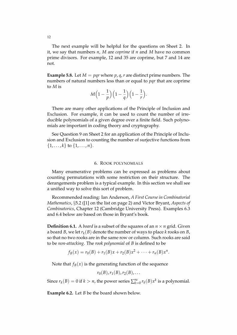
Example 6.2. Let B be the board shown below.
137. (Probleme des Menages.) Let Bm denote the board with exactly m squares in the
sequence shown below.
, , , , , , . . .
(a) Prove that the rook polynomial of Bm is
k
m− k + 1
k
xk.
[Corrected from
m−kk
on 3 November. Hint: there is a very short
proof using the result on lion caging in Problem 5 of Sheet 1. AlternativelyLemma 7.6 can be used to give an inductive proof.]
(b) Find the number of ways to place 8 non-attacking rooks on the unshadedsquares of the board shown below.
(c) At a dinner party eight married couples are to be seated around a circulartable. Men and women must sit in alternate places, and no-one may sit nextto their spouse. In how many ways can this be done? [Hint: first seat thewomen, then use (b) to count the number of ways to seat the men.]
(a) Number the squares in Bm from 1 in the top-left to m in the bottom-right. Aplacement of k rooks on Bm is non-attacking if and only if no two rooks are put insquares with consecutive numbers. The number of such placements is therefore given byQuestion 5 on Sheet 1.
(b) Let B be the board formed from the shaded squares. The polynomial of B can befound using Lemma 7.6, deleting the square in the bottom left: it is
rB(x) = rB15(x) + xrB13(x).
By (a) the coefficient of xk in rB(x) is
15 + 1− k
k
+
13 + 1− (k − 1)
k − 1
=
16− k
k
+
15− k
k − 1
.
By Problem 1, Sheet 1 we have (16− k)15−kk−1
= k
16k
, hence
16− k
k
+
15− k
k − 1
=
16− k
k
+
k
16− k
16− k
k
=
16− k
k
16
16− k.
7
The rook polynomial of B is 1 + 5x + 6x2 + x3.
Exercise: Let B be a board. Show that r0(B) = 1 and that r1(B) is thenumber of squares in B.
Example 6.3. After the recent spate of cutbacks, only four professorsremain at the University of Erewhon. Prof. W can lecture courses 1 or 4;Prof. X is an all-rounder and can lecture 2, 3 or 4; Prof. Y refuses tolecture anything except 3; Prof. Z can lecture 1 or 2. If each professormust lecture exactly one course, how many ways are there to assignprofessors to courses?
Example 6.4. How many derangements σ of 1, 2, 3, 4, 5 have the prop-erty that σ(i) 6= i + 1 for 1 ≤ i ≤ 4?
Lemma 6.5. The rook polynomial of the n× n board isn
∑k=0
k!(
nk
)2xk.
The two following lemmas are very useful when calculating rookpolynomials. Lemma 6.6 will be illustrated with an example in lectures,and proved later using Theorem 9.1 on convolutions of generating func-tions (see Example 9.3).
Lemma 6.6. Let C be a board. Suppose that the squares in C can be partitionedinto sets A and B so that no square in A lies in the same row or column as asquare of B. Then
fC(x) = fA(x) fB(x).
This is the first of many times that multiplying generating functionswill help us to solve combinatorial problems.
Lemma 6.7. Let C be a board and let s be a square in C. Let D be the boardobtained from B by deleting s and let E be the board obtained from B by deletingthe entire row and column containing s. Then
fC(x) = fD(x) + x fE(x).
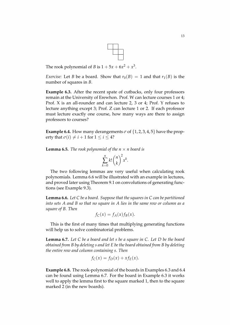
Example 6.8. The rook-polynomial of the boards in Examples 6.3 and 6.4can be found using Lemma 6.7. For the board in Example 6.3 it workswell to apply the lemma first to the square marked 1, then to the squaremarked 2 (in the new boards).

14
1
2
Our final result on rook polynomials is often the most useful in prac-tice. The proof uses the Principle of Inclusion and Exclusion. The fol-lowing lemma isolates the key idea. Its proof needs the same idea weused in Lemma 5.4(ii) to count permutations with a specified set of fixedpoints.
Lemma 6.9. Let B be a board contained in an n× n grid and let 0 ≤ k ≤ n.The number of ways to place k red rooks on B and n− k blue rooks anywhereon the grid, so that the n rooks are non-attacking, is rk(B)(n− k)!.
Theorem 6.10. Let B be a board contained in an n× n grid. Let B denote theboard formed by all the squares in the grid that are not in B. The number ofways to place n non-attacking rooks on B is
n!− (n− 1)!r1(B) + (n− 2)!r2(B)− · · ·+ (−1)nrn(B).
As an easy corollary we get our third proof of the derangements for-mula (Corollary 2.5), that
dn = n!(
1− 11!
+12!− · · ·+ (−1)n
n!
).
See Problem Sheet 3 for some other applications of Theorem 6.10.
Theorem 6.10 is one of the harder results in the course. If you find theproof difficult, you may find the following exercise helpful.
Exercise: Let n = 3 and let B be the board formed by the shaded squaresbelow.
Draw the rook placements lying in each of the sets A∅, A1, A2, A3,A1,2, A1,3, A2,3, A1,2,3 defined in the proof of Theorem 6.10, andcheck the main claim in the proof for k = 0, 1, 2, 3. For instance, fork = 1, you should find that |A1| + |A2| + |A3| is the number ofnon-attacking placements with one red rook on B and two blue rooksanywhere on the grid; according to Lemma 6.9 there are r1(B)(3− 1)!such placements.
15
Part B: Generating Functions
7. INTRODUCTION TO GENERATING FUNCTIONS
Generating functions can be used to solve the sort of recurrence re-lations that often arise in combinatorial problems. But better still, theycan help us to think about combinatorial problems in new ways andsuggest new results.
Definition 7.1. The ordinary generating function associated to the sequencea0, a1, a2, . . . is the power series
∞
∑n=0
anxn = a0 + a1x + a2x2 + · · · .
To indicate that F(x) is the ordinary generating function of the se-quence a0, a1, a2, . . . we may use the notation in §2.2 of Wilf generating-functionology and write
(an)og f←−→ F(x).
Usually we shall drop the word ‘ordinary’ and just write ‘generatingfunction’.
If there exists N ∈ N such that an = 0 if n > N, then the generatingfunction of the sequence a0, a1, a2, . . . is a polynomial. Rook polynomi-als (see Definition 6.1) are therefore generating functions.
OPERATIONS ON GENERATING FUNCTIONS. Let F(x) = ∑∞n=0 anxn and
G(x) = ∑∞n=0 bnxn be generating functions. From
F(x) + G(x) =∞
∑n=0
(an + bn)xn
and
F(x)G(x) =∞
∑n=0
cnxn
where cn = ∑nm=0 ambn−m. The derivative of F(x) is
F′(x) =∞
∑n=0
nxn−1.
Note that if (an)og f←−→ F(x) and (bn)
og f←−→ G(x) then
(an + bn)og f←−→ F(x) + G(x).
The sequence (cn) such that (cn)og f←−→ F(x)G(x) often arises in combi-
natorial problems. This was seen for rook polynomials in Lemma 6.6,and will be studied in §9.

16
It is also possible to define 1/F(x) whenever a0 6= 0. By far the mostimportant case is the case F(x) = 1− x, when
11− x
=∞
∑n=0
xn
is the usual formula for the sum of a geometric progression.
ANALYTIC AND FORMAL INTERPRETATIONS. There are at least two waysto think of a generating function ∑∞
n=0 anxn. Either:
• As a formal power series with x acting as a place-holder. Thisis the ‘clothes-line’ interpretation (see the first page of Wilf gen-eratingfunctionology), in which we regard the power-series as aconvenient way to display the terms in our sequence.
• As a function of a real or complex variable x convergent when|x| < r, where r is the radius of convergence of ∑∞
n=0 anxn.
The formal point of view is often the most convenient because it al-lows us to define and manipulate power series by the operations on theprevious page without worrying about convergence. From this point ofview,
0! + 1!x + 2!x2 + 3!x3 + · · ·is a perfectly respectable formal power series, even though it only con-verges when x = 0. The analytic point of view is useful for provingasymptotic results.1
All the generating functions one normally encounters have positiveradius of convergence, so in practice, the two approaches are equiv-alent. For a more careful discussion of these issues and the generaldefinition of 1/F(x), see §2.1 of Wilf generatingfunctionology.
TWO EXAMPLES OF GENERATING FUNCTIONS.
Example 7.2. What is the generating function for the number of waysto tile a 2× n path with bricks that are either 1× 2 ( ) or 2× 1 ( )?
See the exercise on page 19 for how to extract a formula for the num-ber of tilings from the generating function.
1From the analytic perspective, the formula for the derivative F′(x) on the pre-vious page expresses a non-trivial theorem, namely that power series are differen-tiable functions, with derivatives given by term-by-term differentiation. A similarremark applies to the formulae for the sum F(x) + G(x) and product F(x)G(x).
17
In the second example we shall use products of power series to givea proof of Corollary 3.8 [corrected from Corollary 3.7, 5th November]that is logically independent of Part A. (We assume n = 3, to make thenotation simpler, but once you understand this case, you should seethat the general case is no harder.)
Example 7.3. Let k ∈ N0. Let bk be the number of 3-tuples (t1, t2, t3)such that t1, t2, t3 ∈ N0 and t1 + t2 + t3 = k. Then
∞
∑k=0
bkxk =1
(1− x)3
and so bk = (k+22 ).
USEFUL POWER SERIES. To complete Example 7.3 we needed a specialcase of the result below, which was proved on Question 4 of Sheet 3.
Theorem 7.4. If n ∈ N then
1(1− x)n =
∞
∑k=0
(n + k− 1
k
)xk
A more general result is stated below.
Theorem 7.5 (Binomial Theorem for general exponent). If α ∈ R then
(1 + y)α =∞
∑k=0
α(α− 1) . . . (α− (k− 1))k!
yk
for all y such that |y| < 1.
Exercise: Let α ∈ Z.
(i) Show that if α ≥ 0 then Theorem 7.4 agrees with the Bino-mial Theorem for integer exponents, proved in Theorem 3.6, andwith Theorem 7.5.
(ii) Show that if α < 0 then Theorem 7.4 agrees with Question 5 onSheet 3. (Substitute −x for y.)
We shall need the case α = 1/2 of the general Binomial Theorem tofind the Catalan Numbers in §9.
As we saw in Example 7.3, geometric series often arise in generatingfunctions problem. So you need to get used to spotting either side ofthe identity 1/(1− rx) = ∑∞
n=0 rnxn. The exponential series, exp x =
∑∞n=0
xn
n! , is also often useful.

18
8. RECURRENCE RELATIONS AND ASYMPTOTICS
We have seen that combinatorial problems often lead to recurrencerelations. For example, in §2 we found the derangement numbers dnby solving the recurrence relation in Theorem 2.4. See also Questions 5and 7 on Sheet 1 for other examples.
Generating functions are very useful for solving recurrence relations.The method is clearly explained at the end of §1.2 of Wilf generating-functionology. Given a recurrence satisfied by the sequence a0, a1, a2, . . .proceed as follows:
(a) Use the recurrence to write down an equation satisfied by thegenerating function F(x) = ∑∞
n=0 anxn;
(b) Solve the equation to get a closed form for the generating func-tion;
(c) Use the closed form for the generating function to find a formulafor the coefficients.
Step (a) will become routine with practice. To obtain terms like nan−1,try differentiating F(x). Powers of x will usually be needed to get ev-erything to match up correctly. In Step (c) it is often necessary to usepartial fractions.
Example 8.1. Solve an+2 = 5an+1 − 6an for n ∈ N0 subject to the initialconditions a0 = A, a1 = B.
Another way to proceed is to first rewrite the recurrence as an =5an−1 − 6an−2 for n ≥ 2; then the shifts are done by multiplication by xand x2 rather than division.
The next theorem gives a general form for the partial fraction expres-sions needed to solve these recurrences, Recall that if
f (x) = cdxd + cd−1xd−1 + · · ·+ c0
and cd 6= 0 then f is said to have degree d; we write this as deg f = d.This theorem will not be proved in lectures: see instead Chapter 25 ofBiggs Discrete Mathematics ([2] in the list of recommended reading).
Theorem 8.2. Let f (x) and g(x) be polynomials with deg f < deg g. If
g(x) = α(x− 1/β1)d1 . . . (x− 1/βk)
dk
where α, β1, β2, . . . , βk are distinct non-zero complex numbers and d1, d2, . . . ,dk ∈ N, then there exist polynomials P1, . . . , Pk such that deg Pi < di and
f (x)g(x)
=P1(1− β1x)(1− β1x)d1
+ · · ·+ Pk(1− βkx)(1− βkx)dk
where Pi(1− βix) is Pi evaluated at 1− βix.
19
Theorem 7.4 can then be used to find the coefficient of xn in f (x)/g(x).If di = 1 for all i then each polynomial Pi is just a constant Bi ∈ C andTheorem 8.2 states that
f (x)g(x)
=B1
1− β1x+ · · ·+ Bk
1− βkx.
In this case the coefficient of xn in f (x)/g(x) is B1βn1 + · · ·+ Bkβn
k .
When f (x)/g(x) is a generating function for a sequence a0, a1, a2, . . .it is usually easiest to use values of the sequence to determine any un-known constants.
Example 8.3. Will solve bn = 3bn−1 − 4bn−3 for n ≥ 3.
The next exercise completes the solution to Example 7.2.
Exercise: In Example 7.2 we saw that if an is the number of ways to tilea a 2× n path with bricks that are either 1× 2 ( ) or 2× 1 ( ), thenan = an−1 + an−2, and that the generating function
F(x) =∞
∑n=0
anxn
satisfies (1− x− x2)F(x) = 1. Show that x2 + x− 1 = (x− φ)(x− ψ)
where φ = −1+√
52 and ψ = −1−
√5
2 . Show that 1/φ = −ψ and 1/ψ =−φ and deduce from Theorem 8.2 that
an = C(1 +
√5
2
)n+ D
(1−√
52
)n
for some C, D ∈ C. Find C and D by using the values a0 = a1 = 1 andsolving a pair of simultaneous equations. (Or by some other methodfor finding partial fractions, if we prefer.) You should get
C =12+
12√
5and D =
12− 1
2√
5.
In §2 we used the recurrence dn = (n− 1)(dn−1 + dn−2) for the de-rangement numbers to prove Theorem 2.5 by induction on n. This re-quired us to already know the formula. Generating functions give amore systematic approach. (You are asked to fill in the details in thisproof in Question 2 on Sheet 4.)
Theorem 8.4. Let pn = dn/n! be the probability that a permutation of the set1, 2, . . . , n, chosen uniformly at random, is a derangement. Then
npn = (n− 1)pn−1 + pn−2
for all n ≥ 2 and
pn = 1− 11!
+12!− · · ·+ (−1)n
n!.
20
The steps needed in this proof can readily be performed using com-puter algebra packages. Indeed, MATHEMATICA implements a morerefined version of our three step programme for solving recurrences inits RSolve command. (See the discussion in Appendix A of Wilf gener-atingfunctionology.)
It is usually possible to get some information about the asymptoticgrowth of a sequence from its generating function. For this, it is es-sential to use the analytic interpretation, and think of the generatingfunction as a function defined on the complex numbers.
In the theorem below, a singularity of G is a point where G is unde-fined. (This is a bit loose, but will do for this overview.) For example, ifG(z) = 1/(1− z) then the unique singularity of G is at z = 1.
Theorem 8.5. Let F(z) = ∑∞n=0 anzn be the generating function for the se-
quence a0, a1, a2, . . .. Let z0 be the singularity of F(z) of smallest modulus andlet R = |z0|. For any ε > 0 we have
|an| ≤( 1
R+ ε)n
for all sufficiently large n ∈ N.
See §2.4 in Wilf generatingfunctionology for a proof of Theorem 8.4. Theproofs of this theorem, and Theorem 8.2, are non-examinable, but youmight be asked to apply these results in simple cases
Example 8.6. Let an be the number of tilings defined in Example 8.1.We saw that the generating function for an is F(x) = 1/(1− x − x2).The singularity of F(x) of least modulus is at z0 = −1+
√5
2 . Since 1/z0 =1+√
52 , it follows from Theorem 8.5 that given any ε > 0, we have
an ≤(1 +
√5
2+ ε)n
for all sufficiently large n ∈ N. From the exact formula for an, it ispossible to get a more precise result: an is always the closest integer toC( 1+
√5
2)n, where C is as defined in the exercise after Example 8.3.
If F(z) has no singularities then the conclusion of Theorem 8.5 holdsfor any R ∈ R≥0.
Example 8.7. Let G(z) = ∑∞n=0 pnzn be the generating function for the
proportion of permutations of 1, 2, . . . , n that are derangements. Wesaw that
G(z) =exp(−z)
1− z.

21
A direct application of Theorem 8.5 gives only that pn ≤ 1/(1− ε)n forall sufficiently large n. (Why is this uninteresting?) In such cases, it is agood idea to take out the part of the function that causes G(z) to blowup. Define g(z) by
G(z) =e−1
1− z+ g(z).
Then we can extend g to a function defined on all of C. Using the exten-sion to Theorem 8.5 just mentioned, it follows that |pn − e−1| < 1/10n
for all sufficient large n. (Here 10 is just one possible choice of R.)
Note that we got this result in Example 8.6 without using the exactformula for the pn. This is important because in trickier problems wemight know the generating function, but not have an exact formula forits coefficients.
9. CONVOLUTIONS AND THE CATALAN NUMBERS
The problems in this section fit into the following pattern: supposethatA, B and C are classes of combinatorial objects and that each objecthas a size in N0. Write size(X) for the size of X. Suppose that there arefinitely many objects of any given size.
Let an, bn and cn denote the number of objects of size n in A, B, C,respectively.
Theorem 9.1. Suppose there is a bijection between objects Z ∈ C of size n andpairs of objects (X, Y) such that X ∈ A and Y ∈ B and size(X) + size(Y) =n. Then
∞
∑n=0
cnxn =( ∞
∑n=0
anxn)( ∞
∑n=0
bnxn)
The critical step in the proof is to show that
cn = a0bn + a1bn−1 + · · ·+ an−1b1 + anb0 =n
∑m=0
ambn−m.
If sequences (an), (bn) and (cn) satisfy this relation then we say that (cn)is the convolution of (an) and (bn).
Example 9.2. The grocer sells indistinguishable apples and bananas inunlimited quantities.
(a) What is the generating function for the number of ways to buy npieces of fruit if bananas are only sold in bunches of three?
(b) How would your answer to (a) change if dates are also sold?
(c) What if dates are unavailable, but apples come in two varieties?
22
It would also be possible to do (b) directly, by using a more generalversion of Theorem 9.1 where the objects are decomposed into three (ormore) subobjects.
Example 9.3. Lemma 6.6 on rook placements states that if C is a boardthat A and B where no square in A lies in the same row or column as asquare in B has a very short proof using Theorem 9.1.
Exercise: Show tha splitting a non-attacking placement of rooks on Cinto the placements on the sub-boards A and B gives a bijection satisfy-ing the hypotheses of Theorem 9.1. (Define the size of a rook placementand the sets A, B, C.) Hence prove Lemma 6.6.
The canonical application of convolutions is to the Catalan numbers.These numbers have many different combinatorial interpretations; weshall define them using rooted binary trees drawn in the plane.
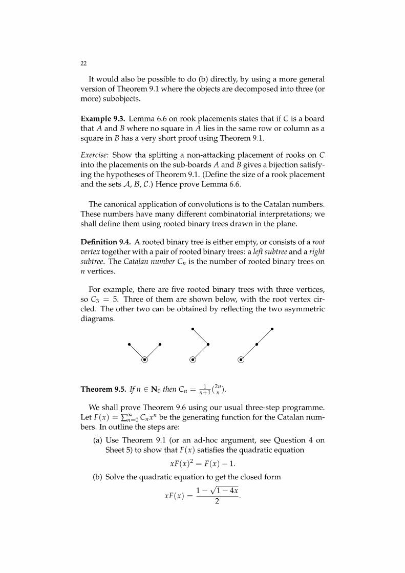
Definition 9.4. A rooted binary tree is either empty, or consists of a rootvertex together with a pair of rooted binary trees: a left subtree and a rightsubtree. The Catalan number Cn is the number of rooted binary trees onn vertices.
For example, there are five rooted binary trees with three vertices,so C3 = 5. Three of them are shown below, with the root vertex cir-cled. The other two can be obtained by reflecting the two asymmetricdiagrams.
18
10. Convolutions and the Catalan numbers
Definition 10.1. The convolution of the sequences a0, a1, a2, . . . andb0, b1, b2, . . . is the sequence c0, c1, c2, . . . defined by
cn =n
k=0
akbn−k.
Keeping the notation from the definition, let F (x) =∞
n=0 anxn,
let G(x) =∞
n=0 bnxn and let H(z) =
∞n=0 cnx
n. By definition of theproduct of formal power series, we have F (x)G(x) = H(x). This makesgenerating functions ideal for finding sequences defined by convolutions.
Convolutions frequently arise in combinatorial problems. See Prob-lem Sheet 4 for some more examples.
Example 10.2. Given a pile of indistinguishable building blocks, howmany ways are there to use n blocks to make an equilateral triangleand a square?
The canonical application of convolutions is to the Catalan numbers.These numbers have a huge number of combinatorial interpretations;we shall define them using rooted binary trees drawn in the plane.
Definition 10.3. A rooted binary tree is either empty, or consists of aroot vertex together with a pair of rooted binary trees: a left subtreeand a right subtree. The Catalan number Cn is the number of rootedbinary trees on n vertices.
For example, there are five rooted binary trees with three vertices,so C3 = 5. Corrected from the wrong C4 = 5. Three of themare shown below, with the root vertex circled. The other two can beobtained by reflection.
Lemma 10.4. If n ∈ N then
Cn = C0Cn−1 + C1Cn−2 + · · · + Cn−2C1 + Cn−1C0.
Theorem 10.5. If n ∈ N0 then Cn = 1n+1
2nn
.
Theorem 9.5. If n ∈ N0 then Cn = 1n+1(
2nn ).
We shall prove Theorem 9.6 using our usual three-step programme.Let F(x) = ∑∞
n=0 Cnxn be the generating function for the Catalan num-bers. In outline the steps are:
(a) Use Theorem 9.1 (or an ad-hoc argument, see Question 4 onSheet 5) to show that F(x) satisfies the quadratic equation
xF(x)2 = F(x)− 1.
(b) Solve the quadratic equation to get the closed form
xF(x) =1−√
1− 4x2
.

23
(c) Use the general version of the Binomial Theorem in Theorem 7.5to deduce the formula for Cn.
The Catalan Numbers have a vast number of combinatorial interpre-tations. See Question 4 on Sheet 6 for one more. A further 64 (andcounting) are given in Exercise 6.19 in Stanley Enumerative Combina-torics II, CUP 2001.
Exercise: Explain the unusual structure of the decimal expansion
12 −
√14 − 1
1000 = 0.001 001 002 005 014 042 . . . .
As a further application of convolutions we will give yet anotherproof (probably the shortest yet!) of the formula for the derangementnumbers dn.
Lemma 9.6. If n ∈ N0 thenn
∑k=0
(nk
)dn−k = n!.
The sum in the lemma becomes a convolution after a small amountof rearranging.
Theorem 9.7. If G(x) = ∑∞n=0 dmxm/m! then
G(x) exp(x) =1
1− x.
It is now easy to deduce the formula for dn; the argument needed isthe same as the final step in the proof of Theorem 8.4. The generatingfunction G used above is an example of an exponential generating func-tion.
10. PARTITIONS
Definition 10.1. A partition of a number n ∈ N0 is a sequence of naturalnumbers (λ1, λ2, . . . , λk) such that
(i) λ1 ≥ λ2 ≥ · · · ≥ λk ≥ 1.(ii) λ1 + λ2 + · · ·+ λk = n.
The entries in a partition λ are called the parts of λ. Let p(n) be thenumber of partitions of n.
By this definition the unique partition of 0 is the empty partition ∅,and so p(0) = 1. The sequence of partition numbers begins
1, 1, 2, 3, 5, 7, 11, 15, . . . .

24
Example 10.2. Let an be the number of ways to pay for an item costing npence using only 2p and 5p coins. Equivalently, an is the number ofpartitions of n into parts of size 2 and size 5. Will find the generatingfunction for an.
The next theorem can be proved using a generalized version of Theo-rem 9.1 in which a partition of n decomposes into subobjects consistingof its parts of size 1, its parts of size 2, and so on.
Instead we will give a direct proof that repeats the main idea in The-orem 9.1.
Theorem 10.3. The generating function for p(n) is∞
∑n=0
p(n)xn =1
(1− x)(1− x2)(1− x3) . . ..
It is often useful to represent partitions by Young diagrams. The Youngdiagram of (λ1, . . . , λk) has k rows of boxes, with λi boxes in row i. Forexample, the Young diagram of (6, 3, 3, 1) is
.
The next theorem has a very simple proof using Young diagrams. (Seealso Question 9 on Sheet 5.)
Theorem 10.4. Let n ∈ N and let k ≤ n. The number of partitions of n intoparts of size ≤ k is equal to the number of partitions of n with at most k parts.
While there are bijective proofs of the next theorem using Young di-agrams, it is much easier to prove it using generating functions. Notehow we adapt the proof of Theorem 10.3 to get the generating functionsfor two special types of partitions.
Theorem 10.5. Let n ∈ N. The number of partitions of n with at most onepart of any given size is equal to the number of partitions of n into odd parts.
For a generalization of this result see Question 9 on Sheet 6.
There are many deep combinatorial and number-theoretic propertiesof the partition numbers. For example, in 1919 Ramanujan used ana-lytic arguments with generating functions to prove that
p(4), p(9), p(14), p(19), . . . , p(5m + 4), . . .
25
are all divisible by 5. In 1944 Freeman Dyson found a bijective proofof this result while still an undergraduate. A number of deep gener-alizations of Ramanujan’s congruences have since been proved, mostrecently by Mahlburg in 2005.
Many easily stated problems remain open: for example, is p(n) evenabout half the time?
The problem of finding an estimate for the size of the partition num-ber p(n) was solved in 1919 by Hardy and Ramanujan as the originalapplication of the circle method. The crudest version of their result is
p(n) ∼ ec√
n
4n√
3
where c = 2√
π2
6 , and ∼ means that the ratio of the two sides tendsto 1 as n → ∞. For a more elementary result, that helps to explainthe constant c in the Hardy–Ramanujan theorem, see Question 10 onSheet 6. It is an open problem to find an entirely combinatorial proofthat there is a constant A such that p(n) < A
√n for all n ∈ N.
25
Part C: Ramsey Theory
11. INTRODUCTION TO RAMSEY THEORY
A typical result in Ramsey Theory says that any sufficiently largecombinatorial structure always contain a substructure with some reg-ular pattern. For example, any infinite sequence of real numbers con-tains either an increasing or a decreasing subsequence (the Bolzano–Weierstrass theorem). The finite version of this result will appear onProblem Sheet 7.
Most of the results in Ramsey Theory are naturally stated in terms ofgraphs. In this course we will concentrate on the finite case.
Definition 11.1. A graph consists of a set V of vertices together with aset E of 2-subsets of V called edges. The complete graph with vertex set Vis the graph whose edge set is all 2-subsets of V.
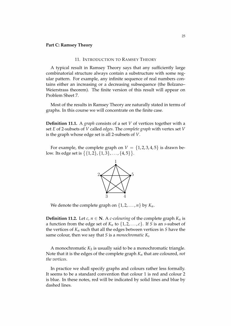
For example, the complete graph on V = 1, 2, 3, 4, 5 is drawn be-low. Its edge set is
1, 2, 1, 3, . . . , 4, 5
.
24
Part C: Ramsey Theory
13. Introduction to Ramsey Theory
The idea behind Ramsey theory is that any sufficiently large struc-ture should contain a substructure with some regular pattern. Forexample, any infinite sequence of real numbers contains either an in-creasing or a decreasing subsequence (the Bolzano–Weierstrass theo-rem).
Most of the results in this area concern graphs: we shall concentrateon the finite case.
Definition 13.1. A graph is a set X of vertices together with a set Eof 2-subsets of X called edges. The complete graph on X is the graphwhose edge set is all 2-subsets of X.
For example, the complete graph on 5 vertices is drawn below. Itsedge set is
1, 2, 1, 3, . . . , 4, 5
.
1
2
3 4
5
We denote the complete graph with n vertices by Kn. The graph K3
is often called a triangle.
Exercise: Find the number of edges in Kn.
Definition 13.2. Let c ∈ N and let G be a complete graph, with edgeset E. A c-colouring of G is a function from E to 1, 2, . . . , c. If Y isan r-set of vertices of G such that all edges between vertices in Y havethe same colour, then we say that Y is a monochromatic Kr.
Note that it is the edges that are coloured, not the vertices.
In practice we shall specify graphs and colourings rather less formally.It seems to be a standard convention that colour 1 is red, colour 2 isblue and colour 3 (which we won’t need for a while) is green.
Example 13.3. In any two-colouring of the edges of K6, there is eithera red triangle, or a blue triangle.
We denote the complete graph on 1, 2, . . . , n by Kn.
Definition 11.2. Let c, n ∈ N. A c-colouring of the complete graph Kn isa function from the edge set of Kn to 1, 2, . . . , c. If S is an s-subset ofthe vertices of Kn such that all the edges between vertices in S have thesame colour, then we say that S is a monochromatic Ks
A monochromatic K3 is usually said to be a monochromatic triangle.Note that it is the edges of the complete graph Kn that are coloured, notthe vertices.
In practice we shall specify graphs and colours rather less formally.It seems to be a standard convention that colour 1 is red and colour 2is blue. In these notes, red will be indicated by solid lines and blue bydashed lines.

26
Exercise: Show that in the colouring of K6 below there is a unique blue(dashed) K4 and exactly two red (solid) triangles. Find all the blue tri-angles.
1
2 3
4
56
Example 11.3. In any red-blue colouring of the edges of K6 there is ei-ther a red triangle or a blue triangle.
Definition 11.4. Given s, t ∈ N, with s, t ≥ 2, we define the Ramseynumber R(s, t) to be the smallest n (if one exists) such that in any red-blue colouring of the complete graph on n vertices, there is either ared Ks or a blue Kt.
For example, we know from Example 11.3 that R(3, 3) ≤ 6.
Lemma 11.5. Let s, t ∈ N with s, t ≥ 2. Let N ∈ N. Assume that R(s, t)exists.
(i) If N ≥ R(s, t) then in any red-blue colouring of KN there is either ared Ks or a blue Kt.
(ii) If N < R(s, t) there exist colourings of KN with no red Ks or blue Kt.
By Question 2 on Sheet 6 there is a red-blue colouring of K5 with nomonochromatic triangle. Hence, Lemma 11.5(i), R(3, 3) > 5. It nowfollows from Example 11.3 that R(3, 3) = 6.
Exercise: Let s, t ∈ N with s, t ≥ 2. Show that R(s, t) = R(t, s).
We will prove in Theorem 12.3 that all the two-colour Ramsey num-bers R(s, t) exist, and that R(s, t) ≤ (s+t−2
s−1 ). (Please do not assume thisresult when doing Sheet 6.)
One family of Ramsey numbers is easily found.
Lemma 11.6. If s ≥ 2 then R(s, 2) = R(2, s) = s.

27
The main idea need to prove Theorem 12.3 appears in the next exam-ple.
Example 11.7. In any two-colouring of K10 there is either a red K3 or ablue K4. Hence R(3, 4) ≤ 10.
This bound can be improved using a result from graph theory. Recallthat if v is a vertex of a graph G then the degree of v is the number ofedges of G that meet v.
Lemma 11.8 (Hand-Shaking Lemma). Let G be a graph with vertex set1, 2, ..., n and exactly e edges. If di is the degree of vertex i then
2e = d1 + d2 + · · ·+ dn.
Theorem 11.9. R(3, 4) = 9.
The proof of the final theorem is left to you: see Question 1 on Sheet 7.
Theorem 11.10. R(4, 4) ≤ 18.
There is a red-blue colouring of K17 with no red K4 or blue K4 soR(4, 4) = 18. A construction is given in Question 8 of Sheet 7.
It is a very hard problem to find the exact values of Ramsey num-bers for larger s and t. For a survey of other known results on R(s, t)for small s and t, see Stanislaw Radziszowski, Small Ramsey Numbers,Electronic Journal of Combinatorics, available at www.combinatorics.org/Surveys. For example, it was shown in 1965 that R(4, 5) = 25, butall that is known about R(5, 5) is that it lies between 43 and 49. It isprobable that no-one will ever know the exact value of R(6, 6).
12. RAMSEY’S THEOREM
Since finding the Ramsey numbers R(s, t) exactly is so difficult, wesettle for proving that they exist, by proving an upper bound for R(s, t).We work by induction on s + t. The following lemma gives the criticalinductive step.
Lemma 12.1. Let s, t ∈ N with s, t ≥ 3. If R(s− 1, t) and R(s, t− 1) existthen R(s, t) exists and
R(s, t) ≤ R(s− 1, t) + R(s, t− 1).
Theorem 12.2. For any s, t ∈ N with s, t ≥ 2, the Ramsey number R(s, t)exists and
R(s, t) ≤(
s + t− 2s− 1
).

28
We now get a bound on the diagonal Ramsey numbers R(s, s). Notethat because of the use of induction on s+ t, we could not have obtainedthis result without first bounding all the Ramsey numbers R(s, t).
Corollary 12.3. If s ∈ N and s ≥ 2 then
R(s, s) ≤(
2s− 2s− 1
)≤ 4s−1.
One version of Stirling’s Formula states that if m ∈ N then√
2πm(m
e)m ≤ m! ≤
√2πm
(me)me1/12m.
These bounds lead to the asymptotically stronger result that
R(s, s) ≤ 4s√
sfor all s ∈ N.
Corollary 12.3 was proved by Erdos and Szekeres in 1935. We havefollowed their proof above. The strongest improvement known to dateis due to David Conlon, who showed in 2004 that, up to a rather tech-nical error term, R(s, s) ≤ 4s/s. In 1947 Erdos proved the lower boundR(s, s) ≥ 2(s−1)/2. His argument becomes clearest when stated in prob-abilistic language: we will see it in Part D of the course.
To end this introduction to Ramsey Theory we give some related re-sults.
PIGEONHOLE PRINCIPLE. The Pigeonhole Principle states that if n pi-geons are put into n − 1 holes, then some hole must contain two ormore pigeons. See Question 8 on Sheet 6 for some applications of thePigeonhole Principle.
In Examples 11.3 and 11.6, and Lemma 12.1, we used a similar result:if r + s − 1 objects (in these cases, edges) are coloured red and blue,then either there are r red objects, or s blue objects. This is probably thesimplest result that has some of the general flavour of Ramsey theory.
MULTIPLE COLOURS. It is possible to generalize all the results provedso far to three or more colours.
Theorem 12.4. There exists n ∈ N such that if the edges of Kn are colouredred, blue and yellow then there exists a monochromatic triangle.
There are (at least) two ways to prove Theorem 12.4. The first adaptsour usual argument, looking at the edges coming out of vertex 1 andconcentrating on those vertices joined by edges of the majority colour.The second uses a neat trick to reduce to the two-colour case.

29
Part D: Probabilistic Methods
13. REVISION OF DISCRETE PROBABILITY
This section is intended to remind you of the definitions and lan-guage of discrete probability theory, on the assumption that you haveseen most of the ideas before. These notes are based on earlier notes byDr Barnea and Dr Gerke; of course any errors are my responsibility.
For further background see any basic textbook on probability, for ex-ample Sheldon Ross, A First Course in Probability, Prentice Hall 2001.
Definition 13.1.• A probability measure p on a finite set Ω assigns a real number pω
to each ω ∈ Ω so that 0 ≤ pω ≤ 1 for each ω and
∑ω∈Ω
pω = 1.
We say that pω is the probability of ω.• A probability space is a finite set Ω equipped with a probability
measure. The elements of a probability space are sometimescalled outcomes.• An event is a subset of Ω.• The probability of an event A ⊆ Ω, denoted P[A] is the sum of
the probability of the outcomes in A; that is
P[A] = ∑ω∈A
pω.
It follows at once from this definition that P[ω] = pω for each ω ∈Ω. We also have P[∅] = 0 and P[Ω] = 1.
Example 13.2(1) To model a throw of a single unbiased die, we take
Ω = 1, 2, 3, 4, 5, 6and put pω = 1/6 for each outcome ω ∈ Ω. The event that wethrow an even number is A = 2, 4, 6 and as expected, P[A] =p2 + p4 + p6 = 1/6 + 1/6 + 1/6 = 1/2.
(2) To model a throw of a pair of dice we could take
Ω = 1, 2, 3, 4, 5, 6 × 1, 2, 3, 4, 5, 6and give each element of Ω probability 1/36, so p(i,j) = 1/36for all (i, j) ∈ Ω. Alternatively, if we know we only care aboutthe sum of the two dice, we could take Ω = 2, 3, . . . , 12 withp2 = 1/36, p3 = 2/36, . . . , p6 = 5/36, p7 = 6/36, p8 = 5/36,. . . , p12 = 1/36. The former is natural and more flexible.
30
(3) A suitable probability space for three flips of a coin is
Ω = HHH, HHT, HTH, HTT, THH, THT, TTH, TTTwhere H stands for heads and T for tails, and each outcome hasprobability 1/8. To allow for a biased coin we fix 0 ≤ q ≤ 1and instead give an outcome with exactly k heads probabilityqk(1− q)3−k.
(4) Let n ∈ N and let Ω be the set of all permutations of 1, 2, . . . , n.Set pσ = 1/n! for each permutation σ ∈ Ω. This gives a suitablesetup for Theorem 2.6. Later we shall use the language of prob-ability theory to give a shorter proof of part (ii) of this theorem.
It will often be helpful to specify events (i.e. subsets of Ω) a littleinformally. For example, in (3) above we might write P[at least twoheads], rather than P[HHT, HTH, THH, HHH].
UNIONS, INTERSECTIONS AND COMPLEMENTS. Let Ω be a probabilityspace. If A, B ⊆ Ω then
P[A ∪ B] = ∑ω∈A∪B
pω = ∑ω∈A
pω + ∑ω∈B
pω − ∑ω∈A∩B
pω
= P[A] + P[B]− P[A ∩ B].
In particular, if A and B are disjoint, i.e. A ∩ B = ∅, then P[A ∪ B] =P[A] + P[B]. The complement of an event A ⊆ Ω is defined to be
A = ω ∈ Ω : ω 6∈ A.Since
1 = P[Ω] = P[A ∪ A] = P[A] + P[A]
we have P[A] = 1− P[A].
Exercise: Show that if A1, . . . , An ⊆ Ω then
P[A1 ∪ · · · ∪ An] ≤ P[A1] + · · ·+ P[An].
CONDITION PROBABILITY AND INDEPENDENCE.
Definition 13.3. Let Ω be a probability space, and let A, B ⊆ Ω beevents.
• If P[B] 6= 0 then we define the conditional probability of A given Bby
P[A|B] = P[A ∩ B]P[B]
.
• The events A, B are said to be independent if P[A∩B] = P[A]P[B].

31
Suppose that each element of Ω has equal probability p. Then
P[A|B] = |A ∩ B|p|B|p =
|A ∩ B||B|
is the proportion of elements of B that also lie in A; informally, if weknow that the event B has occurred, then the probability that A has alsooccurred is P[A|B].
Exercise: Show that if A and B are events in a probability space suchthat P[A], P[B] 6= 0, then P[A|B] = P[A] if and only if A and B areindependent.
Conditional probability can be quite subtle.
Exercise: Let Ω = HH, HT, TH, TT be the probability space for twoflips of a fair coin, so each outcome has probability 1
4 . Let A be the eventthat both flips are heads, and let B be the event that at least one flip is ahead. Write A and B as subsets of Ω and show that P[A|B] = 1/3.
Example 13.4 (The Monty Hall Problem). On a game show you are of-fered the choice of three doors. Behind one door is a car, and behind theother two are goats. You pick a door and then the host, who knows wherethe car is, opens another door to reveal a goat. You may then either openyour original door, or change to the remaining unopened door. Assum-ing you want the car, should you change?
Most people find the answer to the Monty Hall problem a little sur-prising. The Sleeping Beauty Problem, stated below, is even more con-troversial.
Example 13.5. Beauty is told that if a coin lands heads she will be wokenon Monday and Tuesday mornings, but after being woken on Mondayshe will be given an amnesia inducing drug, so that she will have nomemory of what happened that day. If the coin lands tails she willonly be woken on Tuesday morning. At no point in the experimentwill Beauty be told what day it is. Imagine that you are Beauty and areawoken as part of the experiment and asked for your credence that thecoin landed heads. What is your answer?
The related statistical issue in the next example is also widely misun-derstood.
Example 13.6. Suppose that one in every 1000 people has disease X.There is a new test for X that will always identify the disease in anyonewho has it. There is, unfortunately, a tiny probability of 1/250 that thetest will falsely report that a healthy person has the disease. What isthe probability that a person who tests positive for X actually has thedisease?

32
RANDOM VARIABLES.
Definition 13.7. Let Ω be a probability space. A random variable on Ω isa function X : Ω→ R.
Definition 13.8. If X, Y : Ω→ R are random variables then we say thatX and Y are independent if for all x, y ∈ R the events
A = ω ∈ Ω : X(ω) = x and
B = ω ∈ Ω : Y(ω) = yare independent.
The following shorthand notation is very useful. If X : Ω → R isa random variable, then ‘X = x’ is the event ω ∈ Ω : X(ω) = x.Similarly ‘X ≥ x’ is the event ω ∈ Ω : X(ω) ≥ x. We mainly use thisshorthand in probabilities, so for instance
P[X = x] = P[ω ∈ Ω : X(ω) = x
].
Exercise: Show that X, Y : Ω→ R are independent if and only if
P[(X = x) ∩ (Y = y)] = P[X = x]P[Y = y]
for all x, y ∈ R. (This is just a trivial restatement of the definition.)
Example 13.9. Let Ω = HH, HT, TH, TT be the probability space fortwo flips of a fair coin. Define X : Ω → R to be 1 if the first coin isheads, and zero otherwise. So
X(HH) = X(HT) = 1 and X(TH) = X(TT) = 0.
Define Y : Ω→ R similarly for the second coin.
(i) The random variables X and Y are independent.(ii) Let Z be 1 if exactly one flip is heads, and zero otherwise. Then
X and Z are independent, and Y and Z are independent.(iii) There exist x, y, z ∈ 0, 1 such that
P[X = x, Y = y, Z = z] 6= P[X = x]P[Y = y]P[Z = z].
This shows that one has to be quite careful when defining indepen-dence for a family of random variables. (Except in the Lovasz LocalLemma, we will be able to manage with the pairwise independence de-fined above.)
Given random variables X, Y : Ω → R we can define new randomvariables by taking functions such as X + Y, aX for a ∈ R and XY. For
33
instance (X + Y)(ω) = X(ω) + Y(ω), and so on. Notice that if z ∈ Rthen
ω ∈ Ω : (X + Y)(ω) = z =⋃
x+y=zω ∈ Ω : X(ω) = x, Y(ω) = y.
The events above are disjoint for different x, y, so we get
P[X + Y = z] = ∑x+y=z
P[(X = x) ∩ (Y = y)].
If X and Y are independent then
P[(X = x) ∩ (Y = y)] = P[X = x]P[Y = y]
and soP[X + Y = z] = ∑
x+y=zP[X = x]P[Y = y].
(Note that all of these sums have only finitely many non-zero sum-mands, so they are well-defined.)
Exercise: Show similarly that if X, Y : Ω → R are independent randomvariables then
P[XY = z] = ∑xy=z
P[X = x]P[Y = y].
EXPECTATION AND LINEARITY.
Definition 13.10. Let Ω be a probability space with probability mea-sure p. The expectation E[X] of a random variable X : Ω→ R is definedto be
E[X] = ∑ω∈Ω
X(ω)pw.
Intuitively, the expectation of X is the average value of X on elementsof Ω, if we choose ω ∈ Ω with probability pω. We have
E[X] = ∑ω∈Ω
X(ω)pω = ∑x∈R
∑ω
X(ω)=x
xpω = ∑x∈R
xP[X = x].
A critical property of expectation is that it is linear. Note that we do notneed to assume independence in this lemma.
Lemma 13.11. Let Ω be a probability space. If X1, X2, . . . , Xk : Ω→ R arerandom variables then
E[a1X1 + a2X2 + · · ·+ akXk] = a1E[X1] + a2E[X2] + · · ·+ akE[Xk]
for any a1, a2, . . . , ak ∈ R.
34
Proof. By definition the left-hand side is
∑ω∈Ω
pω
(a1X1 + · · ·+ akXk)(ω) = ∑
ω∈Ωpω
(a1X1(ω) + · · ·+ akXK(ω)
)
= a1 ∑ω∈Ω
pωX1(ω) + · · ·+ ak ∑ω∈Ω
Xk(ω)
which is the right-hand side.
When X, Y : Ω → R are independent random variables, there is avery useful formula for E[XY].
Lemma 13.12. If X, Y : Ω → R are independent random variables thenE[XY] = E[X]E[Y].
Exercise: Prove Lemma 13.11 by arguing that
E[XY] = ∑z∈R
zP[XY = z] = ∑z∈R
z ∑xy=z
P[(X = x) ∩ (Y = y)]
and using independence.
VARIANCE.
Definition 13.13. Let Ω be a probability space. The variance Var[X] of arandom variable X : Ω→ R is defined to be
Var[X] = E[(X− E[X])2].
The variance measures how much X can be expected to depart fromits mean value E[X]. So it is a measure of the ‘spread’ of X.
It is tempting to define the variance as E[X − E[X]
], but by linearity
this expectation is E[X]− E[X] = 0. One might also consider the quan-tity E
[ ∣∣X− E[X]∣∣ ], but the absolute value turns out to be hard to work
with. The definition above works well in practice.
Lemma 13.14. Let Ω be a probability space.(i) If X : Ω→ R is a random variable then
Var[X] = E[X2]− (E[X])2.
(ii) If X, Y : Ω→ R are independent random variables then
Var[X + Y] = Var[X] + Var[Y].
Exercise: Show that (ii) can fail if X and Y are not independent. [Hint:usually a random variable is not independent of itself.]
35
14. INTRODUCTION TO PROBABILISTIC METHODS
In this section we shall solve some problems involving permutations(including, yet again, the derangements problem) using probabilisticarguments. We shall use the language of probability spaces and randomvariables recalled in §13. It will be particularly important for you to askquestions if the use of anything from this section is unclear.
Throughout this section we fix n ∈ N and let Ω be the set of allpermutations of the set 1, 2, . . . , n. We define a probability measureq : Ω → R by qσ = 1/n! for each permutation σ of 1, 2, . . . , n. Thismakes Ω into a probability space in which all the permutations haveequal probability. We say that the permutations are chosen uniformly atrandom.
Recall that, in probabilistic language, events are subsets of Ω.
Exercise: Let x ∈ 1, 2, . . . , n and let Ax = σ ∈ Ω : σ(x) = x.Then Ax is the event that a permutation fixes x. What is the probabilityof Ax?
Building on this we can give a better proof of Theorem 2.6(ii).
Theorem 14.1. Let F : Ω → N0 be defined so that F(σ) is the number offixed points of the permutation σ ∈ Ω. Then E[F] = 1.
To give a more general result we need cycles and the cycle decompo-sition of a permutation.
Definition 14.2. A permutation σ of 1, 2, . . . , n acts as a k-cycle on ak-subset S ⊆ 1, 2, . . . , n if S has distinct elements x1, x2, . . . , xk suchthat
σ(x1) = x2, σ(x2) = x3, . . . , σ(xk) = x1.If σ(y) = y for all y ∈ 1, 2, . . . , n such that y 6∈ S then we say that σ isa k-cycle, and write
σ = (x1, x2, . . . , xk).
Note that there are k different ways to write a k-cycle. For example,the 3-cycle (1, 2, 3) can also be written as (2, 3, 1) and (3, 1, 2).
Definition 14.3. We say that cycles (x1, x2, . . . , xk) and (y1, y2, . . . , y`)are disjoint if
x1, x2, . . . , xk ∩ y1, y2, . . . , y` = ∅.
Lemma 14.4. A permutation σ of 1, 2, . . . , n can be written as a composi-tion of disjoint cycles. The cycles in this composition are uniquely determinedby σ.

36
The proof of Lemma 14.4 is non-examinable and will not be given infull in lectures. What is more important is that you can apply the result.We shall use it below in Theorem 14.5
Exercise: Write the permutation of 1, 2, 3, 4, 5, 6 defined by σ(1) = 3,σ(2) = 4, σ(3) = 1, σ(4) = 6, σ(5) = 5, σ(6) = 2 as a composition ofdisjoint cycles.
Given a permutation σ of 1, 2, . . . , n and k ∈ N, we can ask: whatis the probability that a given x ∈ 1, 2, . . . , n lies in a k-cycle of σ? Thefirst exercise in this section shows that the probability that x lies in a1-cycle is 1/n.
Exercise: Check directly that the probability that 1 lies in a 2-cycle of apermutation of 1, 2, 3, 4 selected uniformly at random is 1/4.
Theorem 14.5. Let 1 ≤ k ≤ n and let x ∈ 1, 2, . . . , n. The probabilitythat x lies in a k-cycle of a permutation of 1, 2, . . . , n chosen uniformly atrandom is 1/n.
Theorem 14.6. Let pn be the probability that a permutation of 1, 2, . . . , nchosen uniformly at random is a derangement. Then
pn =pn−2
n+
pn−3
n+ · · ·+ p1
n+
p0
n.
It may be helpful to compare this result with Lemma 9.7: there weget a recurrence by considering fixed points; here we get a recurrenceby considering cycles.
We now use generating functions to recover the usual formula for pn.
Corollary 14.7. For all n ∈ N0,
pn = 1− 11!
+12!− 1
3!+ · · ·+ (−1)n
n!.
We can also generalize Theorem 14.1.
Theorem 14.8. Let Ck : Ω → R be the random variable defined so thatCk(σ) is the number of k-cycles in the permutation σ of 1, 2, . . . , n. ThenE[Ck] = 1/k for all k such that 1 ≤ k ≤ n.
Note that if k > n/2 then a permutation can have at most one k-cycle. So in these cases, E[Ck] is the probability that a permutation of1, 2, . . . , n, chosen uniformly at random, has a k-cycle.
37
15. RAMSEY NUMBERS AND THE FIRST MOMENT METHOD
The grandly named ‘First Moment Method’ is nothing more than thefollowing simple observation.
Lemma 15.1 (First Moment Method). Let Ω be a probability space and letM : Ω→ N0 be a random variable taking values in N0. If E[M] = x then
(i) P[M ≥ x] > 0, so there exists ω ∈ Ω such that M(ω) ≥ x.(ii) P[M ≤ x] > 0, so there exists ω′ ∈ Ω such that M(ω′) ≤ x.
Exercise: Check that the lemma holds in the case when
Ω = 1, 2, 3, 4, 5, 6 × 1, 2, 3, 4, 5, 6models the throw of two fair dice (see Example 13.2(2)) and if (α, β) ∈ Ωthen M(α, β) = α + β.
The kth moment of a random variable X is defined to be E[Xk]. Some-times stronger results can be obtained by considering higher moments.We shall concentrate on first moments, where the power of the methodis closely related to the linearity property of expectation (see Lemma13.11).
Our applications will come from graph theory.
Definition 15.2. Let G be a graph with vertex set V. A cut (S, T) of G isa partition of V into subsets A and B. The capacity of a cut (S, T) is thenumber of edges of G that meet both S and T.
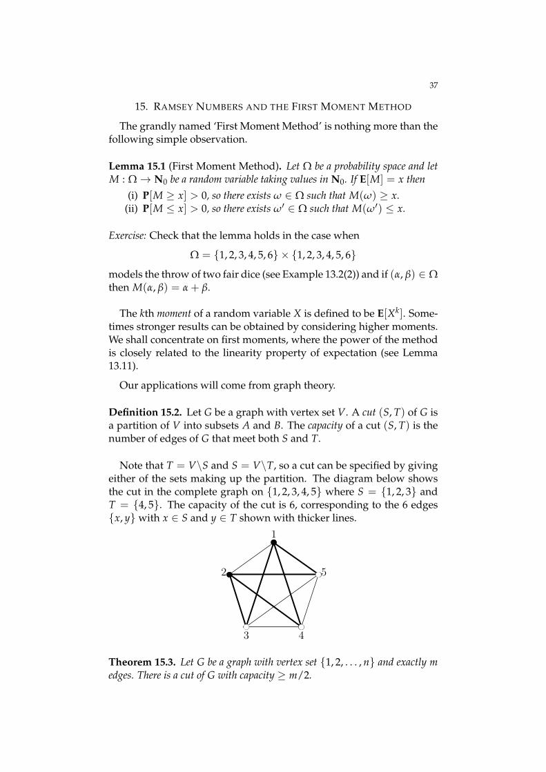
Note that T = V\S and S = V\T, so a cut can be specified by givingeither of the sets making up the partition. The diagram below showsthe cut in the complete graph on 1, 2, 3, 4, 5 where S = 1, 2, 3 andT = 4, 5. The capacity of the cut is 6, corresponding to the 6 edgesx, y with x ∈ S and y ∈ T shown with thicker lines.
31
18. Ramsey Numbers and the First Moment Method
The grandly named ‘First Moment Method’ is nothing more thanthe following observation.
Lemma 18.1 (First Moment Method). Let Ω be a probability spaceand let X : Ω→ N0 be a random variable. If E[X] = x then
(i) P[X ≥ x] > 0, so there exists ω ∈ Ω such that X(ω) ≥ x.(ii) P[X ≤ x] > 0, so there exists ω ∈ Ω such that X(ω) ≤ x.
Exercise: check that the lemma holds in the case where
Ω = 1, 2, 3, 4, 5, 6× 1, 2, 3, 4, 5, 6models the throw of two fair dice and X(x, y) = x + y.
More generally, the k-th moment of X is E[Xk]. Sometimes strongerresults can be obtained by considering these higher moments. We shallconcentrate on first moments, where the power is the method is closelyrelated to the linearity property of expectation (see Lemma 16.8).
Our applications will come from graph theory.
Definition 18.2. Let G be a graph with vertex set V . A cut of G is apartition of V into two disjoint subsets A and B. The capacity of thecut is the number of edges of G that meet both A and B.
Note that B = V \A and A = V \B, so a cut can be specified bygiving either of the sets in the partition.
For example, the diagram below shows the cut in the complete graphon 1, 2, 3, 4, 5 where A = 1, 2, 3 and B = 4, 5. The capacity ofthis cut is 6, corresponding to the 6 edges x, y for x ∈ A, y ∈ Bshown with thicker lines.
1
2
3 4
5
Theorem 18.3. Let G be a graph with n vertices and m edges. Thereis a cut of G with capacity ≥ m/2.
Theorem 15.3. Let G be a graph with vertex set 1, 2, . . . , n and exactly medges. There is a cut of G with capacity ≥ m/2.
38
In 1947 Erdos proved a lower bound on the Ramsey Numbers R(s, s)that is still almost the best known result in this direction. Our version ofhis proof will use the First Moment Method in the following probabilityspace.
Lemma 15.4. Let n ∈ N and let Ω be the set of all red-blue colourings of thecomplete graph Kn. Let pω = 1/|Ω| for each ω ∈ Ω. Then
(i) each colouring in Ω has probability 1/2(n2);
(ii) given any m edges in G, the probability that all m of these edges havethe same colour is 21−m.
Theorem 15.5. Let n ∈ N and let s ∈ N with s ≥ 2. If(
ns
)21−(s
2) < 1
then there is a red-blue colouring of the complete graph on 1, 2, . . . , n withno red Ks or blue Ks.
Corollary 15.6. For any s ∈ N with s ≥ 2 we have
R(s, s) ≥ 2(s−1)/2.
For example, since(
428
)21−(8
2) ≈ 0.879 < 1,
if we repeatedly colour the complete graph on 1, 2, ..., 42 at random,then we will fairly soon get a colouring with no monochromatic K8.However, to check that we have found such a colouring, we will have tolook at all (42
8 ) ≈ 1.18× 10⁸ subsets of 1, 2, . . . , 42. Thus Theorem 15.5does not give an effective construction.
It is a major open problem to find, for each s ≥ 2, an explicit colour-ing of the complete graph on 1.01s vertices with no monochromatic Ks.(Here 1.01 could be replaced with 1 + ε for any ε > 0.
The bound in Corollary 15.6 can be slightly improved by the LovaszLocal Lemma: see the final section.
39
16. LOVASZ LOCAL LEMMA
The section is non-examinable, and is included for interest only.
In the proof of Theorem 15.5, we considered a random colouringof the complete graph on 1, 2, . . . , n and used Lemma 15.1 to showthat, provided (n
s)21−(s
2) < 1 there was a positive probability that thiscolouring had no monochromatic Ks. As motivation for the Lovasz Lo-cal Lemma, consider the following alternative argument, which avoidsthe use of Lemma 15.1.
Alternative proof of Theorem 15.5. As before, let Ω be the probability spaceof all colourings of the complete graph on 1, 2, . . . , n, where eachcolouring gets the same probability. For each s-subset
S ⊆ 1, 2, . . . , n,let ES be the event that S is a monochromatic Ks. The event that no Ksis monochromatic is then
⋂S ES, where the intersection is taken over all
s-subsets S ⊆ 1, 2, . . . , n and ES = Ω\ES. So it will suffice to showthat P[
⋂ES] > 0, or equivalently, that P[
⋃ES] < 1.
In lectures we used Lemma 15.4 to show that if S is any s-subset of1, 2, . . . , n then
P[ES] = 21−(ns).
By the exercise on page 30, the probability of a union of events is at mostthe sum of their probabilities, so
P[⋃
SES] ≤
(ns
)21−(n
s).
Hence the hypothesis implies that P[⋃
S ES]< 1, as required.
If the events ES were independent, we would have
P[⋂
SES]= ∏
SP[ES].
Since each event ES has non-zero probability, it would follow that theirintersection has non-zero probability, giving another way to finish theproof. However, the events are not independent, so this is not an ad-missible strategy. The Lovasz Local Lemma gives a way to get aroundthis obstacle.
We shall need the following definition.
Definition 16.1. An event E is mutually independent of a collection A ofevents, if for all U ⊆ A and U′ ⊆ A\U we have
P[
E∣∣∣( ⋂
C∈UC)∩( ⋂
D∈U′D)]
= P[E]

40
whenever(⋂
C∈U C)∩(⋂
D∈U′ D)
is non-empty.
For example, if the events ES are as defined above, then ES is inde-pendent of the events ET : |S ∩ T| ≤ 1. This can be checked quiteeasily: informally the reason is that since each S ∩ T has at most onevertex, no edge is common to both S and T, and so knowing whetheror not T is monochromatic gives no information about S.
Lemma 16.2 (Symmetric Lovasz Local Lemma). Let d ∈ N. Let A be acollection of events such that P[E] ≤ p for all E ∈ A. Suppose that for eachevent E ∈ A, there is a subset AE of A such that
(i) |AE| ≥ |A| − d;(ii) E is independent of AE.
If ep(d + 1) ≤ 1 then
P[ ⋂
E∈AE]> 0
For a proof of the lemma, see Chapter 5 of Noga Alon and Joel H.Spencer The Probabilistic Method, 3rd edition. A simpler proof of a verysimilar result, where ep(d + 1) is replaced with 4pd, is given in §6.7of Michael Mitzenmacher and Eli Upfal Probability and Computing(see [6] in the list of page 2).
The Lovasz Local Lemma can be used to prove a slightly strongerversion of Theorem 15.5.
Theorem 16.3. Let n, s ∈ N. If
e((s
2
)(n− 2s− 2
)+ 1)
21−(s2) < 1
then there is a red-blue colouring of the complete graph Kn with no red Ks orblue Ks.
Proof. Define the events ES as at the start of this section. We remarkedthat if S is an s-subset of 1, 2, . . . , n then the event ES is independentof the events ET for those s-subsets T such that S ∩ T ≤ 1. There are atmost (
s2
)(n− 2s− 2
)
s-subsets T such that S ∩ T ≥ 2, since we can choose two commonelements in (s
2) ways, and then choose any s− 2 of the remaining n− 2elements of 1, 2, . . . , n to complete T. (There is some over-countinghere, so this is only an upper bound.)
Therefore we let d = (s2)(
n−2s−2). Since
P[ES] = 21−(ns).

41
for all S, we take p = 21−(ns). Then we can apply the Lovasz Local
Lemma, provided that ep(d + 1) ≤ 1, which is one of the hypotheses ofthe theorem. Hence
P[⋂
SES
]> 0
and so there is a red-blue colouring with no monochromatic Ks, as re-quired.
Theorem 16.2 is stronger than Theorem 15.5 when s is reasonablylarge.
Example 16.4. When s = 15, the largest n such that(
n15
)21−(15
2 ) < 1
is n = 792. So Theorem 15.5 tells us that R(15, 15) > 792. But
e((15
2
)(n− 215− 2
)+ 1)
21−(152 ) < 1
provided n ≤ 947. Theorem 16.2 therefore gives the stronger result thatR(15, 15) > 947.
A more general version of the Lovasz Local Lemma can be used toget the bound
R(s, 3) ≥ Cs2
(log s)2
for some constant C. For an outline of the proof and references to fur-ther results, see Alon and Spencer, Chapter 5.