combinatorics - · pdf filecombinatorics henry liu, 15 august 2007 combinatorics is an area of...
TRANSCRIPT

Combinatorics
Henry Liu, 15 August 2007
Combinatorics is an area of mathematics which is not easy to define. Looselyspeaking, it is the area of mathematics which studies discrete structures. It bringstogether many subareas. One of these subareas is the theory of counting objects,where many ideas occur. These ideas include permutations, combinations,factorials, and the use of binomial coefficients. This subarea is more formally knownas enumerative combinatorics. Another subarea, which can be considered as an areain its own right, is graph theory. Roughly speaking, a graph is a structure whichconsists of a set of points, and a set of line segments joining some pairs of the points.We can say a lot of things about such a structure.
Although there are many more subareas of combinatorics, in this set ofnotes we shall just focus on these two, since they occur the most often in olympiadmathematics. We shall also have another section here, which discusses a very usefulidea: we shall see how to prove the impossibility of certain statements, by meansof taking a colouring, with finitely many colours, of a certain structure. This isequivalent to partitioning our structure into finitely many parts, and we can deduceresults from such partitions.
Combinatorics is an area which is hardly visible at schools. Some of the ideaswhich are well exposed are the simplest ones, such as factorials, some of the ideasinvolving the binomial coefficient, and maybe some basic graph theory at A-level.It is an area which must be learnt outside the classroom.
So, we shall prove many basic theorems here. We will only leave the proof of onetheorem: Turan’s Theorem, as an exercise. This is because a proof of this result israther technical. The completion of a proof is denoted by the symbol �.
1. Enumerative Combinatorics: Counting Objects
Many problems in combinatorics involve counting objects. In this section, wediscuss many ideas related to such problems.
1.1 Permutations and Combinations
Definition 1 Let n ∈ N. Then, we define n!, read n factorial, to be the number
n! = 1× 2× 3× · · · × (n− 1)× n.
We also define 0! = 1.
Now, given n ∈ Z, n ≥ 0 and 0 ≤ r ≤ n, we would like to know: “How manyways can we choose r objects out of n objects, subject to certain conditions?”. Theconditions include whether we care about the order in which we pick the objects,whether the objects are distinct, and whether we can choose the objects more thanonce. We first distinguish the cases whether ordering matters or not.
1

Definition 2 Let n ∈ Z, n ≥ 0 and 0 ≤ r ≤ n. If we have n objects, then asubset of r objects where the ordering matters is an r-permutation of the objects. Ifordering does not matter, then the subset is an r-combination.
In particular, when r = n, an n-permutation is simply called a permutation.
Remark. For r = 0 in either case, we choose none of the objects. We definea 0-permutation or a 0-combination simply to be the empty set. This must be thecase when n = 0.
We first consider r-permutations. We would like to count how many of thesethere are from n objects, under certain conditions. Firstly, we consider the casewhen the objects are distinct, and that we can replace the objects after pickingthem.
Theorem 1 Suppose that we have n ≥ 1 distinct objects. Let 0 ≤ r ≤ n. We pickr of the objects, one at a time, allowing replacement. Then, the number of differentr-permutations is nr. Also, when n = 0, there is exactly one 0-permutation: theempty set.
Remark. Note that, for n ≥ 1 and r = 0 the number of ways of picking nothingis 1, the “empty pick”. This agrees with Theorem 1; when r = 0, we have n0 = 1way of picking nothing. From now on, this “empty pick” will always be counted,unless otherwise stated.
Proof of Theorem 1. There are n ways of picking the first object. Then thereare n ways of picking the second object, since replacement is allowed. Repeatingthis r times, we get nr as the total number of possibilities. �
Example 1. There are 64 = 1296 4-digit numbers which contain the digits 1, 2,3, 4, 5 and 6.
Next, we consider the same question, but not allowing replacement.
Theorem 2 Suppose that we have n ≥ 0 distinct objects. Let 0 ≤ r ≤ n. We pickr of the objects, one at a time, without replacement. Then, the number of differentr-permutations is
n× (n− 1)× · · · × (n− r + 1) =n!
(n− r)!.
Remark. In particular, when r = n, the total number of permutations of ndistinct objects is n!
(n−n)!= n!. Also, when r = 0, we have n!
(n−0)!= 1 0-permutation,
as expected.
Proof of Theorem 2. The result is true for n = 0. For n ≥ 1, we argue asin Theorem 1. We have n choices of picking the first object. After that, we haven − 1 choices, then n − 2 choices, and so on, until we have n − r + 1 choices of
2

picking the rth object, since we are not allowing replacement. So the total numberof possibilities is n× (n− 1)× · · · × (n− r + 1) = n!
(n−r)!. �
Definition 3 The expression n!(n−r)!
is usually denoted by nPr.
Example 2. If n = 5 and r = 2, we have the following 2-permutations of{1, 2, 3, 4, 5}: {1, 2}, {1, 3}, {1, 4}, {1, 5}, {2, 1}, {2, 3}, {2, 4}, {2, 5}, {3, 1}, {3, 2},{3, 4}, {3, 5}, {4, 1}, {4, 2}, {4, 3}, {4, 5}, {5, 1}, {5, 2}, {5, 3} and {5, 4}, giving atotal of 20. This agrees with Theorem 2: 5!
(5−2)!= 20.
Before we proceed, we would like to divert and make a shorthand notation. Theabove listing of r-permutations looks rather cumbersome. We can make such a listinglook a bit more pleasant simply by ignoring the chain brackets, and the commaswithin the r-permutations. This shorthand notation also works for r-combinations.
Definition 4 For an r-permutation or an r-combination {x1, x2, . . . , xr}, we maywrite it as x1x2 · · ·xr
So, the above listing can simply be written as 12, 13, 14, 15, 21, 23, 24, 25, 31,32, 34, 35, 41, 42, 43, 45, 51, 52, 53, 54.
Next, we consider the same question, but when the objects may not be distinct.In this case, we only consider the number of permutations.
Theorem 3 Suppose that we have n ≥ 0 objects, where n1 of them are of type 1,n2 of them are of type 2, . . . , nk of them are of type k, so that n = n1 + · · · + nk.Then, the number of permutations of the objects is
n!
n1!× n2!× · · · × nk!.
Proof. If we disregard that some of the objects are the same, then we wouldhave n! permutations. Now, in each permutation, within the objects of type 1, theycan be permuted in n1! ways; within the objects of type 2, they can be permuted inn2! ways, and so on. So, such a permutation has been counted n1!× n2!× · · · × nk!times, and we must divide n! by n1!× n2!× · · · × nk! to get the correct answer. �
Example 3. Another way of thinking about the situation of Theorem 3 is justthe number of anagrams of a word. For example, there are
11!
1!× 4!× 4!× 2!= 34650
anagrams of the word ‘Mississippi’.
Remark. It is not easy to get a precise expression for the number ofr-permutations in the situation of Theorem 3.
So far, we have been counting the number of r-permutations from n objects,
3

where we care about the ordering in which the chosen objects appear. We now wantto count the number of r-combinations from n objects, so that we do not care aboutthe ordering of the chosen objects. Firstly, Theorem 4 below considers the case whenwe cannot replace an object after picking it. This is the analogue of Theorem 2.
Theorem 4 Suppose that we have n ≥ 0 distinct objects. Let 0 ≤ r ≤ n. We pickr of the objects, without replacement. Then, the number of different r-combinationsis
n!
r!(n− r)!.
Remark. If r = n, there is only one possibility: to choose all n objects. Thisagrees with the expression in Theorem 4: n!
n!(n−n)!= 1. Also, for r = 0, there is one
possibility; to choose nothing. This again agrees with the expression: n!0!(n−0)!
= 1.
Proof of Theorem 4. Simply, if we fix an r-permutation of the objects, wemay permute the r objects in r! ways. Each such r-permutation represents the samer-combination. So the answer is just to divide nPr by r!, giving n!
r!(n−r)!possibilities.
�
Definition 5 The expression n!r!(n−r)!
is usually denoted by nCr, or by(
nr
). It is
called a binomial coefficient and we read it as “n choose r”.
Example 4. There are 10 ways of choosing two numbers from the set {1, 2, 3, 4, 5},the subsets being 12, 13, 14, 15, 23, 24, 25, 34, 35, and 45. This agrees with Theorem4: 5!
2!(5−2)!= 10.
Finally, we want to count the number of r-combinations of n distinct objects,but allowing replacement.
Theorem 5 Suppose that we have n ≥ 0 distinct objects. Let 0 ≤ r ≤ n. We pick rof the objects, allowing replacement. Then, the number of different r-combinationsis
(n+ r − 1)!
r!(n− 1)!=
(n+ r − 1
r
).
Proof. Given such an r-combination, we can code it by a sequence of dotsand dashes as follows. Suppose that the r-combination has r1 objects of type 1,r2 objects of type 2, . . . , rn objects of type n, where 0 ≤ ri ≤ r for each i, andr1 + · · · + rn = r. Now, starting with n − 1 dashes, we place r1 dots to the left ofthe first dash, then r2 dots between the first and second dashes, r3 dots betweenthe second and third dashes, and so on, and rn dots to the right of the last dash.Clearly, this gives a direct correspondence between the r-combinations and all thepossible permutations of r dots and n− 1 dashes. So, we can apply Theorem 3: wehave r + n− 1 objects, r of one type, and n− 1 of another type. The total numberof permutations is therefore (r+n−1)!
r!(n−1)!=(
n+r−1r
). �
4

Example 5. A bakery sells ten types of cakes. The number of ways of choosingfour cakes is
(134
)= 715 (provided that there are at least four of each type of cake
available).
1.2 More on the Binomial Coefficient
In Definition 5, we defined the binomial coefficient(
nr
). In this section, we briefly
digress and discuss some results about these numbers, before we return to discussmore on counting objects.
Definition 6 We define Pascal’s Triangle as follows. We start with a 1, and thisis row 0 of the triangle. A subsequent row is formed as follows. To get an entry inrow i, we add two adjacent entries in row i − 1, and place the sum in the space inrow i which is between and below the two row i− 1 entries. If one of the entries inrow i− 1 is missing, we assign a 0 to the missing spot.
Also, in each row, the entry on the left is the 0th entry of the row, and the entriesto its right are, in order, the 1st entry, the 2nd entry, and so on.
Below are row 0 to row 5 of Pascal’s Triangle.
11 1
1 2 11 3 3 1
1 4 6 4 11 5 10 10 5 1
It is well-known that the entries of Pascal’s Triangle are precisely the binomialcoefficients.
Theorem 6 For n ∈ Z, n ≥ 0 and 0 ≤ r ≤ n, the rth entry in row n of Pascal’striangle is precisely
(nr
).
Proof. We use induction on n. The result is true for n = 0. We only have r = 0,and
(00
)= 1, the only entry in row 0 of the triangle.
Now, let i ≥ 1, and suppose that the result holds for every entry in row i− 1 ofthe triangle. Let 0 ≤ r ≤ i. If 1 ≤ r ≤ i− 1, then the rth entry in row i is(
i− 1
r − 1
)+
(i− 1
r
)=
(i− 1)!
(r − 1)!(i− r)!+
(i− 1)!
r!(i− 1− r)!
=(i− 1)!
(r − 1)!(i− 1− r)!
(1
i− r+
1
r
)=
(i− 1)!
(r − 1)!(i− 1− r)!· i
(i− r)r
=i!
r!(i− r)!=
(i
r
).
5

If r = 0, then the 0th entry in row i of the triangle is
0 +
(i− 1
0
)= 1 =
(i
0
).
If r = i, then the ith entry in row i of the triangle is(i− 1
i− 1
)+ 0 = 1 =
(i
i
).
We have now shown that the result holds for the entries in row i. Hence theresult follows by induction. �
Next, we have the most well-known result involving binomial coefficients, thebinomial theorem.
Theorem 7 (Binomial Theorem) Let x, y ∈ C, and n ∈ Z, n ≥ 0. Then,
(x+ y)n =n∑
r=0
(n
r
)xn−ryr.
Proof. There are many proofs of this result. We give probably the simplest.When we expand out (x + y)n, each term we obtain consists of some x’s and
some y’s multiplied together, the total number of x’s and y’s being n (this is beforewe add any equal terms together). So, it suffices to show that, for each 0 ≤ r ≤ n,there are precisely
(nr
)terms xn−ryr. But this is clear by Theorem 4. We have n
y’s, and we have(
nr
)ways of picking r y’s from them. Whenever we choose r y’s,
we are automatically left with n− r x’s. So we have precisely(
nr
)terms xn−ryr. �
The binomial coefficient also satisfies many properties, and Theorem 8 belowshows some of the most well-known ones.
Theorem 8 Let n ∈ Z, n ≥ 0. We have the following.
(a)(
nr
)=(
nn−r
), if 0 ≤ r ≤ n. Both are equal to n!
r!(n−r)!.
(b)(
n0
)=(
nn
)= 1 if n ≥ 0, and
(n1
)=(
nn−1
)= n if n ≥ 1.
(c)(
nr
)+(
nr+1
)=(
n+1r+1
), if 0 ≤ r ≤ n− 1.
(d)(
n0
)+(
n1
)+(
n2
)+ · · ·+
(nn
)= 2n.
(e)(
n0
)−(
n1
)+(
n2
)− · · ·+ (−1)n
(nn
)= 0.
(f) 1(
n1
)+ 2(
n2
)+ 3(
n3
)+ · · ·+ n
(nn
)= n2n−1.
(g)(
n0
)2+(
n1
)2+(
n2
)2+ · · ·+
(nn
)2=(2nn
).
6

Proof. Properties (a) and (b) are obvious from the definition of(
nr
).
Property (c) has already been proved in the main calculation in the proof ofTheorem 6.
Properties (d) and (e) follow from Theorem 7 by letting x = y = 1 and x = 1,y = −1, respectively.
To get property (f), we let x = 1 in Theorem 7 to get (1 + y)n =∑n
r=0
(nr
)yr.
Differentiating both sides with respect to y gives n(1 + y)n−1 =∑n
r=1 r(
nr
)yr−1.
Then, letting y = 1 gives the result.To get property (g), we consider the coefficient of xn in the expansion of (1+x)2n.
On one hand, this is(2nn
), by Theorem 7. On the other hand, by Theorem 7 again,
we have
(1 + x)2n = (1 + x)n(1 + x)n =
(n∑
r=0
(n
r
)xr
)(n∑
s=0
(n
s
)xs
).
In the product on the right, when we expand, we get a term involving xn wheneverwe multiply a term which involves xt in the first sum by a term which involves xn−t
in the second sum, for some 0 ≤ t ≤ n. For such a t, the corresponding coefficientis(
nt
)(n
n−t
). Summing these coefficients as t varies, and using property (a), we
get that the overall coefficient of xn is also(
n0
)(nn
)+(
n1
)(n
n−1
)+ · · · +
(nn
)(n0
)=(
n0
)2+(
n1
)2+ · · ·+
(nn
)2. This gives property (g). �
In addition to the properties of binomial coefficients given in Theorem 8, thereare many more which are a little bit more complicated.
1.3 Other Ideas on Counting
In this section, we consider some more ideas about counting objects.
1.3.1 Counting Objects in Two Ways
Suppose that we have a certain number of objects. If we are able to count theobjects to sum to the total in two ways, then we have an equation linking twoexpressions, each of which equals the total number of objects.
We have already seen one instance of this idea: when we derived property (g) ofTheorem 8. There, we counted the number of terms involving xn in the expansionof (1 + x)2n, in two ways.
We give another example below. There will be some more examples on this idealater.
Example 6. n real numbers whose sum is n are placed on a circle. Show thatfor any 1 ≤ k ≤ n, some k successive numbers must have a sum at least k.
Let a1, a2, . . . , an be the numbers. We can use the numbers to form an array as
7

follows.a1 a2 a3 · · · an
a2 a3 a4 · · · a1
a3 a4 a5 · · · a2...
......
...ak ak+1 ak+2 · · · an+k−1
Note that the indices are taken modulo n. Now, the total sum of all the numbersin the array is kn, since there are k rows, each with sum n. So, the sum of thecolumns is also kn. Since there are n columns, some column must have a sum ofat least kn
n= k (if every column has sum less than k, then the total sum of the
columns, hence the sum of everything in the array, is less than kn, a contradiction).Moreover, each column represents successive terms on the circle. So we are done.
1.3.2 Bijection Proofs
We now describe a useful technique which can prove statements of the form:
“The number of objects with property A is equal to the number of objectswith property B”.
The idea is that we do not actually try to find the common total number (whichmay be difficult to compute), but we try to ‘match’ the objects with property A tothe objects with property B in a ‘one-on-one’ manner. Such a matching is formallyknown as a bijection.
Definition 7 Let A and B be sets. A function f : A→ B is a bijection if
• for every x, y ∈ A, if x 6= y, then f(x) 6= f(y);
• for every y ∈ B, there exists an x ∈ A such that f(x) = y.
So, going back to the scenario, let A be the set of objects with property A, anddefine B likewise. If we can find a bijection from A to B, then it easily follows that|A| = |B|, provided that the common number is finite. For a problem of such aform, a proof which exhibits a bijection is a ‘bijection proof’.
We will given an example which considers partitions of a number n ∈ N. Weneed to define what a partition is first.
Definition 8 Let n ∈ N. A partition of n is a representation of n as a sum ofpositive integers. Two partitions of n are distinct if the two sets of terms involvedare not equal as multisets. For example, 1 + 1 + 3 and 1 + 3 + 1 represent the samepartition of 5, while 5, 2 + 3 and 4 + 1 represent pairwise distinct partitions of 5.
Remark. So, given n ∈ N, every partition of n is equal to a unique partitionwhere the terms are listed in decreasing order (decreases of zero are possible). So, if
8

we want to list out all the distinct partitions of n, it is a good idea to assume thatthe terms are decreasing in each partition.
Example 7. We prove the following result. For n, r ∈ N with 1 ≤ r ≤ n, thenumber of partitions of n into at most r terms is equal to the number of partitionsof n into any number of terms, each of which is at most r.
Throughout, we assume that all partitions have their terms decreasing. As anexample, for n = 5 and r = 3, the partitions satisfying the former are 3 + 1 + 1,2+2+1, 4+1, 3+2 and 5, while the partitions satisfying the latter are 1+1+1+1+1,2 + 1 + 1 + 1, 3 + 1 + 1, 2 + 2 + 1 and 3 + 2.
We will use a bijection proof to prove the result. For any partition of n, we mayrepresent it by means of a diagram, the Young diagram, or the Ferrers diagram.Figure 1 shows an example of such a diagram, for the partition 5 = 2 + 2 + 1.
.........................................................................................................................................................................................................
.........................................................................................................................................................................................................
.....................................................................................................................................
............
............
............
............
............
............
............
............
............
............
............
.
............
............
............
............
............
............
............
............
............
............
............
.
............
............
............
............
............
............
............
............
............
............
............
.
............
............
............
............
............
......
Figure 1
In a Young diagram, the number of boxes is n. The columns are always decreasingin height from left to right (possibly by zero), and the number of boxes in the columnsare the terms of the partition.
We use this idea to produce a bijection proof. Firstly, it is easy to check thatthe correspondence between the partitions and the Young diagrams of n is bijective(clearly, two different partitions of n map to different Young diagrams, and everyYoung diagram of n is formed from some partition of n). Now, a partition of n withat most r terms has at most r columns in its diagram, while a partition of n, each ofwhose terms is at most r, has a diagram such that every column has height at mostr. So, it is enough to find a bijection between these two classes of Young diagrams.But this is fairly obvious. For a Young diagram of the first type, if we reflect it aboutthe diagonal line at 45◦, we get another Young diagram whose columns have heightsat most r, and so is of the second type. The converse holds as well. Obviously, twodistinct Young diagrams of the first type, when reflected, give two distinct Youngdiagrams of the second type. From these, it is obvious that this ‘reflection’ is therequired bijection, and we are done.
9

For the example where n = 5 and r = 3, we get the bijection
3 + 1 + 1 ←→ 3 + 1 + 1
2 + 2 + 1 ←→ 3 + 2
4 + 1 ←→ 2 + 1 + 1 + 1
3 + 2 ←→ 2 + 2 + 1
5 ←→ 1 + 1 + 1 + 1 + 1
Remark. It is easily conceivable that, for general n and r, the above commonnumber of partitions is difficult to find exactly. This indeed is the case.
1.3.3 Inclusion-Exclusion Principle
When one attempts to count the number of objects, a very common mistakeis usually that some objects are counted too many times. The inclusion-exclusionprinciple is one of the results which can help us to avoid this mistake. Let us lookat a simple example first.
Example 8. A class of students sat a maths exam and an English exam. 18students got a grade A in maths only, 13 students got a grade A in English only,and 5 students got grade A’s in both. How many students got at least one grade A?
If we were just to add the 18 to the 13, we get 31, but we will have counted thosestudents who got grade A’s in both exams twice. So we need to subtract the numberof such students, which is 5. The answer is therefore 18 + 13− 5 = 26 students.
To generalise this, we first define some well-known set operations.
Definition 9 Let A and B be any two sets.
(a) We call the elements which belong to both A and B the intersection of A andB. This set is denoted by A ∩B.
(b) We call the elements which belong to A or B (including both) the union of Aand B. This set is denoted by A ∪B.
(c) We call the elements which belong to A, but not to B, the difference of B fromA. This set is denoted by A \B, or A−B.
Remark. These three operations can obviously extend to more than two sets.But when this happens, if we have at least two of ∩, ∪ and \, or at least two of \involved, we must use brackets to show which operation(s) must be done first. Forexample, ‘A∩B∪C’ does not make sense, since in general, (A∩B)∪C 6= A∩(B∪C).‘A \B \ C’ makes no sense, since (A \B) \ C 6= A \ (B \ C), in general.
However, if we just have ∩ or ∪ on its own, we do not need any brackets, becausein these cases, the set that we get at the end will be the same, no matter which orderwe use for the operations. For example, A∩B∩C makes sense, since (A∩B)∩C =
10

A ∩ (B ∩ C) for any three sets A,B,C, and we use A ∩ B ∩ C for both of these.Similarly for ∪ on its own, and for more than three sets.
So, we can interpret Example 8 in this way. Let A be the set of the studentswho got a grade A in maths, and B be the set of the students who got a grade Ain English. So, we have |A| = 18, |B| = 13 and |A ∩ B| = 5. We want to find thevalue of |A ∪B|. With the same argument as given in the example, we get
|A ∪B| = |A|+ |B| − |A ∩B| = 18 + 13− 5 = 26.
We have now proved the formula
|A ∪B| = |A|+ |B| − |A ∩B|.
Can we extend this formula to three sets? Suppose that we have three sets A,Band C, and we know the values of |A|, |B|, |C|, |A∩B|, |A∩C|, |B∩C| and |A∩B∩C|.Can we find the value of |A ∪B ∪ C|?
We can indeed apply the same argument. If we add |A|, |B| and |C|, we willhave counted the elements of (A ∩ B) \ (A ∩ B ∩ C), (A ∩ C) \ (A ∩ B ∩ C) and(B ∩ C) \ (A ∩ B ∩ C) twice, and the elements of A ∩ B ∩ C three times. Then, ifwe subtract |A∩B|, |A∩C| and |B ∩C|, we will then have counted the elements of(A ∩B) \ (A ∩B ∩C), (A ∩C) \ (A ∩B ∩C) and (B ∩C) \ (A ∩B ∩C) correctly,but we also will have counted the elements of A∩B∩C 3−3 = 0 times. So, adding|A ∩B ∩ C|, we get the correct formula for |A ∪B ∪ C|:
|A ∪B ∪ C| = |A|+ |B|+ |C| − (|A ∩B|+ |A ∩ C|+ |B ∩ C|) + |A ∩B ∩ C|.
This, of course, generalises further to n sets. The result is the inclusion-exclusionprinciple.
Theorem 9 (Inclusion-Exclusion Principle) Let A1, A2, . . . , An be finite sets.Then,
|A1 ∪ A2 ∪ · · · ∪ An| = (|A1|+ |A2|+ · · ·+ |An|)−(|A1 ∩ A2|+ |A1 ∩ A3|+ · · ·+ |An−1 ∩ An|)+(|A1 ∩ A2 ∩ A3|+ |A1 ∩ A2 ∩ A4|+ · · · )− · · ·+(−1)n−1|A1 ∩ A2 ∩ · · · ∩ An|,
where, in the sum on the right, we have the size of every k-wise intersection forevery 1 ≤ k ≤ n, where a k-wise intersection is assigned with the sign (−1)k−1.
Before we prove this, we shall prove a well-known identity about sets.
Lemma 10 Let n ∈ N, n ≥ 3. For sets B1, B2, . . . , Bn, we have
(B1 ∪B2 ∪ · · · ∪Bn−1) ∩Bn = (B1 ∩Bn) ∪ · · · ∪ (Bn−1 ∩Bn).
11
Proof. We first prove that, for three sets A,B,C, we have (A ∪ B) ∩ C =(A ∩ C) ∪ (B ∩ C). We have
x ∈ (A ∪B) ∩ C ⇐⇒ x ∈ A ∪B and x ∈ C⇐⇒ x ∈ A or x ∈ B, and x ∈ C⇐⇒ x ∈ A ∩ C or x ∈ B ∩ C⇐⇒ x ∈ (A ∩ C) ∪ (B ∩ C),
so the identity holds. Now, using this identity repeatedly, we have
(B1 ∪B2 ∪ · · · ∪Bn−1) ∩Bn = [(B1 ∪B2 ∪ · · · ∪Bn−2) ∩Bn] ∪ (Bn−1 ∩Bn)
= [(B1 ∪B2 ∪ · · · ∪Bn−3) ∩Bn]
∪(Bn−2 ∩Bn) ∪ (Bn−1 ∩Bn)
= · · ·= (B1 ∩Bn) ∪ · · · ∪ (Bn−1 ∩Bn).
�
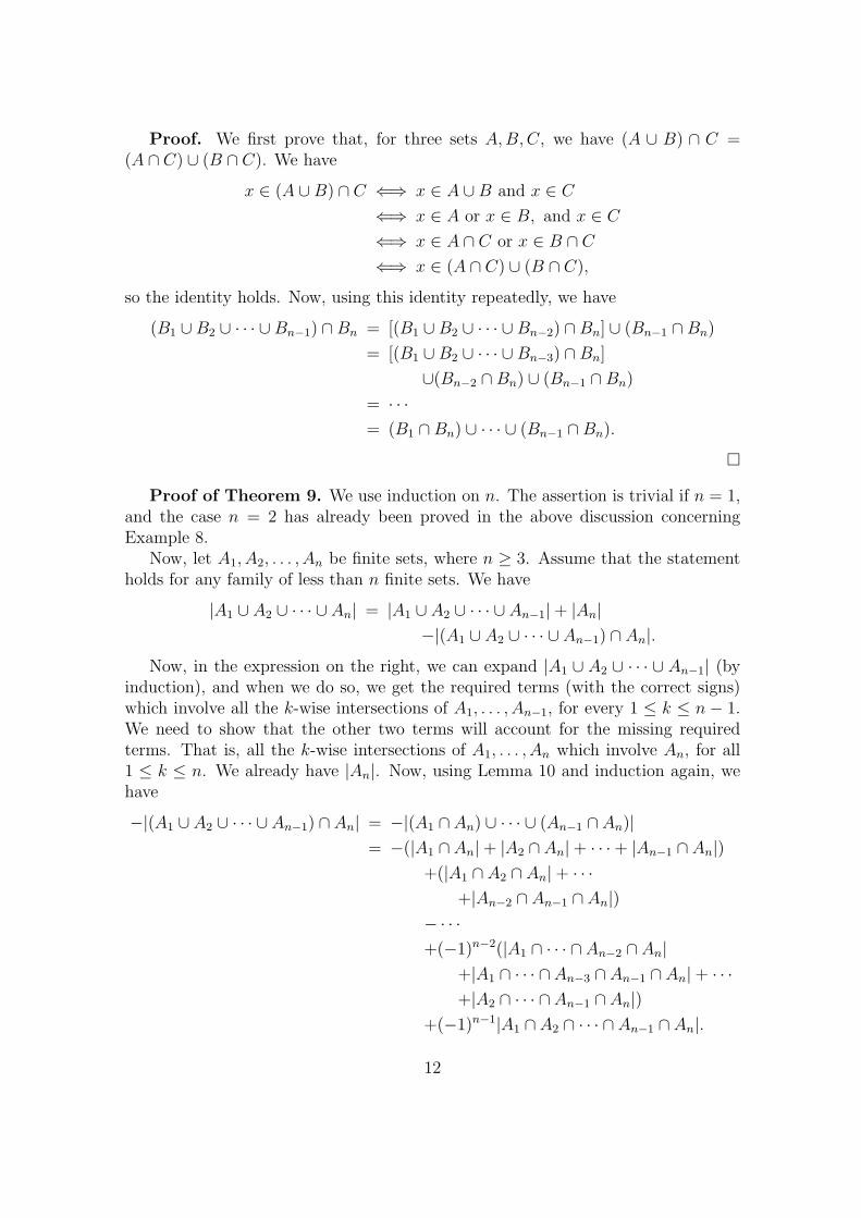
Proof of Theorem 9. We use induction on n. The assertion is trivial if n = 1,and the case n = 2 has already been proved in the above discussion concerningExample 8.
Now, let A1, A2, . . . , An be finite sets, where n ≥ 3. Assume that the statementholds for any family of less than n finite sets. We have
|A1 ∪ A2 ∪ · · · ∪ An| = |A1 ∪ A2 ∪ · · · ∪ An−1|+ |An|−|(A1 ∪ A2 ∪ · · · ∪ An−1) ∩ An|.
Now, in the expression on the right, we can expand |A1 ∪ A2 ∪ · · · ∪ An−1| (byinduction), and when we do so, we get the required terms (with the correct signs)which involve all the k-wise intersections of A1, . . . , An−1, for every 1 ≤ k ≤ n− 1.We need to show that the other two terms will account for the missing requiredterms. That is, all the k-wise intersections of A1, . . . , An which involve An, for all1 ≤ k ≤ n. We already have |An|. Now, using Lemma 10 and induction again, wehave
−|(A1 ∪ A2 ∪ · · · ∪ An−1) ∩ An| = −|(A1 ∩ An) ∪ · · · ∪ (An−1 ∩ An)|= −(|A1 ∩ An|+ |A2 ∩ An|+ · · ·+ |An−1 ∩ An|)
+(|A1 ∩ A2 ∩ An|+ · · ·+|An−2 ∩ An−1 ∩ An|)
− · · ·+(−1)n−2(|A1 ∩ · · · ∩ An−2 ∩ An|
+|A1 ∩ · · · ∩ An−3 ∩ An−1 ∩ An|+ · · ·+|A2 ∩ · · · ∩ An−1 ∩ An|)
+(−1)n−1|A1 ∩ A2 ∩ · · · ∩ An−1 ∩ An|.
12

The final expression consists exactly the missing terms that we needed, with thecorrect signs. �
Example 9. How many positive integers less than 3000 are coprime to 3000?The prime factorisation of 3000 is 3000 = 23 × 3 × 53. Let S be the positive
integers less than 3000, that is, S = {1, 2, . . . , 2999}. We count the number ofelements of S which are not coprime to 3000. The highest common factor of such anumber with 3000 is divisible by at least one of 2, 3 and 5, so such a number must bedivisible by at least one of 2, 3 and 5. Let A be the elements of S which are divisibleby 2, B be the elements of S which are divisible by 3, and C be the elements of Swhich are divisible by 5. We would like to find |A∪B ∪C|, the number of elementsof S which are divisible by at least one of 2, 3 and 5.
We have |A| = |{2, 4, 6, . . . , 2998}| = 1499, |B| = |{3, 6, 9, . . . , 2997}| = 999, and|C| = |{5, 10, 15, . . . , 2995}| = 599. Also, A ∩ B are the elements of S which aredivisible by 6, so |A ∩B| = |{6, 12, 18, . . . , 2994}| = 499. Similarly,
|A ∩ C| = |{10, 20, 30, . . . , 2990}| = 299,
|B ∩ C| = |{15, 30, 45, . . . , 2985}| = 199, and
|A ∩B ∩ C| = |{30, 60, 90, . . . , 2970}| = 99.
So, by the inclusion-exclusion principle, we have
|A ∪B ∪ C| = (1499 + 999 + 599)− (499 + 299 + 199) + 99 = 2199.
This is the number of elements of S which are not coprime to 3000. So thenumber of elements of S which are coprime to 3000 is 2999− 2199 = 800.
1.3.4 Pigeonhole Principle
The simplest case of the pigeonhole principle is that, if we have n boxes and weplace at least n + 1 objects into them, then some box must contain at least twoobjects. This easily generalises to the following result.
Theorem 11 (Pigeonhole Principle) Let n, k ∈ N. Suppose that we place atleast kn+ 1 objects into n boxes. Then some box must contain at least k+ 1 objects.
Proof. Assume not. Then every box has at most k objects, so that the totalnumber of objects is at most kn. This is a contradiction, since we have at leastkn+ 1 objects. �
Theorem 11 is extremely useful, not just in combinatorics, but in just aboutevery branch of mathematics as well.
Example 10. Suppose that we have 10 points within a square of side length 3(including on the edges of the square). Prove that some two points must be within adistance of
√2 of each other.
13
Divide the square into nine 1×1 squares. Then by the pigeonhole principle, sometwo points must lie within one of the squares (including the sides of that square).So we are done, since the longest possible distance between any two such points is√
12 + 12 =√
2.
2. Graph Theory
2.1 Graphs: Definitions
Graphs are very important objects in combinatorics. They are so important thatthere is actually an area of mathematics devoted to them: graph theory (which isa rather large area). Graphs interact very well with other areas of combinatorics.Roughly speaking, a graph is just a set of points, with some pairs of them beingjoined by some lines. Below, we give a more precise definition.
Definition 10 A (simple) graph is a pair G = (V,E), where V is a set, and E isa family of subsets of V , each is of size 2 (and unordered).
An element of V is called a vertex of G, and an element of E is called an edgeof G. V is the vertex set of G, and E is the edge set of G.
Sometimes, we may want to write V (G) = V and E(G) = E, to emphasize thedependence of V and E on G.
We write |G| = |V (G)| and e(G) = |E(G)|, and call these the order and the sizeof the graph G, respectively. Note that each of these can be infinite (we shall seesome examples soon).
The best way to think of a (simple) graph is by a picture. V is a set of points(namely, vertices). E is a set of line or curve segments (namely, edges) joining pairsof vertices such that, a subset of V of size 2 is in E if and only if there is an edgejoining the corresponding two vertices of V .
In this way, we usually use letters like v and u for the vertices of a graph. Foredges, if the edge with end-vertices u and v is in the graph, we just write uv todenote this edge, rather than {u, v}. Note that uv = vu. We may also use letterslike e and f to denote edges.
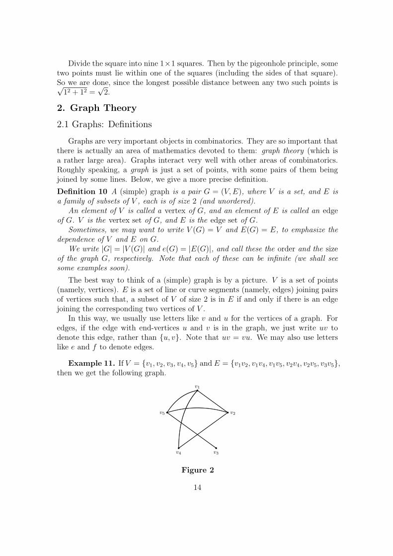
Example 11. If V = {v1, v2, v3, v4, v5} and E = {v1v2, v1v4, v1v5, v2v4, v2v5, v3v5},then we get the following graph.
............
............
.............
.............
...........................................................................................................................................................................................................................
........................................
........................................
........................................
........................................
........................................
.................
........................................
........................................
........................................
........................................
........................................
...............................................................................
............................................................................................................................................................................................................................................
........................................................
..................................
........................................
........................................
........................................
..............
v4 v3
v5 v2
v1
. .
...
Figure 2
14

Remark. We need to be rather careful. We do not allow the following here.
• No ‘loops’ are allowed. That is, a vertex cannot be joined to itself. If we areallowed to have ‘loops’, then we are talking about ‘graphs with loops’.
• No pair of distinct vertices can have more than one edge joining them. If weallow this, then we have ‘multiedges’, and we are talking about ‘multigraphs’.
• The edges are ‘unordered pairs of vertices’. If we care about the ordering ofan edge, we have ‘directed edges’, and we are talking about ‘directed graphs’.
Hence, sometimes we use the word ‘simple’ to emphasize that we do not allowthese things. But here, we will drop this word, since we will only be talking aboutsimple graphs.
However, the edges do not necessarily have to be straight line segments. We canuse curves for edges. But it is absolutely essential to use large dots to show thevertices, because for certain graphs, it may be the case that no matter how we drawthem, we may be forced to have that some edges must cross (this ought to happen ifwe have lots of edges), so that we must declare if there is a vertex at such a positionor not.
Also, the set V can be an infinite set, in which case E can also be infinite. Hereare some examples.
Example 12. We may have V = Z, and E consisting of the edges which joindistinct pairs of even numbers. So, such a graph can only be partially drawn.
Indeed, depending on the vertex set, some graphs may be even harder to draw,maybe impossible. For example, if V = R, and E consists of the edges which joinpairs of real numbers with unit distance between them. We can only barely draw afew vertices and edges of this graph. We can only define it in an abstract way.
Graphs can model many real life situations. For example, a situation where a‘network scenario’ is present. The vertices can represent people and edges can jointwo people if they are related. Or, the vertices can represent computers and theedges can join two computers if they are related in some way. And so on. In thisway, graphs present very nice ways of looking at such a situation.
Now, we define several important classes of graphs, with their notations.
Definition 11 Let n,m ∈ N.
(a) The complete graph on n vertices is the graph with n vertices, where each pairof vertices is joined by an edge. It is denoted by Kn. We have e(Kn) =
(n2
).
(b) The empty graph on n vertices is the graph with n vertices, but with no edges.It is denoted by En. We have e(En) = 0.
15

(c) For n ≥ 3, the cycle on n vertices is the graph with n vertices, v1, v2, . . . , vn
say, with edges v1v2, v2v3, . . . , vn−1vn, vnv1. It is denoted by Cn. We havee(Cn) = n.
(d) The path of length n − 1 is the graph with n vertices, v1, v2, . . . , vn say, withedges v1v2, v2v3, . . . , vn−1vn. It is denoted by Pn−1. We have e(Pn−1) = n− 1.
(e) The complete bipartite graph on m + n vertices is the graph with m + nvertices, u1, u2, . . . , um, v1, v2, . . . , vn say, with edges uivj for every 1 ≤ i ≤ mand 1 ≤ j ≤ n. It is denoted by Km,n. The sets {u1, . . . , um} and {v1, . . . , vn}are the classes of Km,n. We have e(Km,n) = mn.
Figure 3 below shows examples of these graphs.
.....................................................................................................................................
.......................................................................................
........................................
......
........................................
..........................
..................................
...................................................................................
.....................
..........................................................................................................
..............................................................................................................................................
..........................................................................................................
..........................................................................................................
..................................
..................................
..................................
..................................
......
..........................................................................................................
.............................................................................................
.............................................................................................
............
............
............
............
............
............
............
.........
..................................
..................................
..................................
..............................
....................................................................................................................................
............
............
............
............
............
............
............
.........
C5 P3 K2,3E3K4
. ...
.
.. ..
. . .
. .
...
..
..
Figure 3
Next, we consider some properties of a vertex of a graph.
Definition 12 Let G = (V,E) be a graph, and let v ∈ V be a vertex of G.
(a) The vertex u ∈ V is adjacent to v, or is a neighbour of v, if uv ∈ E.
(b) The set of neighbours of v is the neighbourhood of v. This set is denoted byΓ(v). Note that this may be finite or infinite.
(c) The number of neighbours of v is the degree of v, and is denoted by d(v). Notethat d(v) = |Γ(v)|. Again, this may be finite or infinite.
(d) If d(v) = 0, then v is an isolated vertex.
(e) The smallest of all the degrees is the minimum degree of G, and the largest isthe maximum degree of G. These are denoted by δ(G) and ∆(G), respectively.
Sometimes, we may want to write ΓG(v) for Γ(v) and dG(v) for d(v), if we wantto emphasize the dependence of neighbourhood and degree on G.
Remark. If δ(G) and ∆(G) are both finite, then obviously, δ(G) ≤ ∆(G). Also,these quantities are always well-defined, even if the graph G is infinite. It is possibleto have δ(G) =∞ and/or ∆(G) =∞.
We have an elementary result about the sum of the degrees of a graph with finiteorder.
16

Theorem 12 Let G = (V,E) be a graph, with V finite. Let V = {v1, v2, . . . , vn}.Then,
n∑i=1
d(vi) = 2e(G).
So in particular, the sum of the degrees of the vertices of G is always even.
Proof. This is another good example illustrating counting objects in two ways.We count the number of edges of G in two ways. On one hand, this is e(G). Onthe other hand, if we consider summing the degrees of G, then each edge has beencounted exactly twice; an edge uv is counted in the terms d(u) and d(v) of the degreesum. So, e(G) = 1
2
∑ni=1 d(vi), and we are done. �
Now, we define some more properties about graphs themselves. We can talkabout a graph containing other graphs.
Definition 13 Let G = (V,E) be a graph.
(a) A graph H = (V ′, E ′) is a subgraph of G if V ′ ⊆ V and E ′ ⊆ E. We writeH ⊆ G.
(b) Let A ⊆ V . Then the subgraph of G induced by A is the subgraph with vertexset A, and the edges of E whose end-vertices are in A. We write G[A] for thissubgraph.
(c) Let x ∈ V (G). Then the graph G− x is the graph formed by removing x fromG, along with the edges which touch x.
(d) Let e ∈ E(G). Then the graph G − e is the graph (V,E \ {e}). That is, wejust remove the edge e from G.
The above ideas are often useful for proving statements about graphs, when wewant to apply induction on the number of vertices, or on the number of edges (orsome other similar quantity).
Finally, given a graph, it has a ‘complement graph’.
Definition 14 Let G = (V,E) be a graph. The complementary graph of G, or thecomplement of G, is the graph G = (V,E), where E is the complement of E in theset of all possible edges on V .
In other words, to get G from G, we just remove the edges of G, and add backthe edges between vertices of V that were not present in G.
2.2 Bipartite and r-partite Graphs
We shall consider another, rather special, class of graphs. These graphs are ahuge generalisation of the complete bipartite graphs which we have already seen.
17

Definition 15 Let r ∈ N, r ≥ 2. A graph G = (V,E) is an r-partite graph if thereis a partition of V into r parts, V = V1 ∪ V2 ∪ · · · ∪ Vr say, such that for every edgeuv ∈ E, we have u ∈ Vi and v ∈ Vj for some i 6= j. The sets V1, . . . , Vr are theclasses of G.
If G contains every edge between every two classes, then G is a complete r-partitegraph. In the case where all the classes are finite, G is denoted by Kk1,k2,...,kr , whereki = |Vi| for every 1 ≤ i ≤ r, so that k1 + · · · + kr = |V |. We have e(Kk1,k2,...,kr) =∑
i<j kikj.Finally, a 2-partite graph is more commonly called a bipartite graph.
Note that in an r-partite graph, two vertices in the same class cannot be joinedby an edge.
Figure 4 below shows a 4-partite graph, and the graph K4,2,3. The classes in eachcase are shown in the ovals.
.......................................................................................................................................
.......................................................................................................................................
.......................................................................................................................................
.......................................................................................................................................
............................................................................................................................................................................................................................................................................................................................................................................................................................................................................................................................................................
....................................................................................
................................................................................................................................................................................................................................................................................................................
...........................................................................................................................................................................................................
..............................................................................................................................................................................
.........................................................................................................................................................................................
....................................................................................................................................................................
........................................................................................................................................................................................
.........................................................................................................................................................................................
........................................................................................................................................
.............................................................................................................................................................
.........................................................................................................................................................................................................................
...................................................................................................................................................................................................
..........................................................................................................................................................................................................
.................................................................................................................................................................................................
..........................................................................................................................................................
.........................................................................................................................................................................
.....................................................................................................................................................................................
.....................................................................................................................................................................................................
.........................................................................................................................................................................................................
.....................................................................................................................................................................................................................
......................................................................................................................................................
..................................................................................................................................................................................................................................................................................................................................................................................................................................................................
...................................................................................................................................................................................
..........................................................................................
............................................................................................................................................................................................................................................
....................................................................................................................................................................................................................
........................................................................................................................................................................................................................................
....................................................................................................................................................................................................................................................................................................................................................................................................................................................
........................................................................................................
..............................................................................................
.......................................
.......................................................................................................................................................................................................................................................
..................................................................................................................
..........................................................................................................................................................................................................................................................................................................................................................................................................................................
........................................................
........................................................
........................................................
........................................................
..................................
..................................................
..................................................
..................................................
..................................................
..................................................
..
................................................................................................................................................................................................................................
........................................
........................................
........................................
........................................
........................................
............................
............
............
............
............
............
............
............
............
............
............
............
............
............
............
............
......................................................................................................................................................................................................................................................................................................................................................................................................................................................................................................
............................................................................... ................................................................................................................................................................................................................................................................................................................................................................ ..
.
. . ..
...
..
. .
.....
K4,2,3
Figure 4
In certain problems, r-partite graphs, and in particular, bipartite graphs, arevery useful graphs to consider. Here is an example.
Example 13. A group of 13 mathematicians and 6 physicists met at aconference. Many handshakes, all of which involved a mathematician and aphysicist, were made. It is known that everyone has made at least one handshake,that every mathematician made the same number of handshakes, and that the numberof handshakes that every physicist made is a multiple of 3. How many handshakesdid each mathematician make?
Also, describe how the handshakes can be made so that the above scenario can berealised.
This example can be modelled perfectly by a bipartite graph. Let G be such abipartite graph. The classes of G are M and P , where M are the mathematiciansand P are the physicists, so that |M | = 13 and |P | = 6. An edge joins two peopleif they shook hands. For some a ∈ N, we have d(x) = a for every x ∈ M ; notethat our task is to find a. Let P = {p1, . . . , p6}. For some b1, . . . , b6 ∈ N, we haved(pi) = 3bi for every 1 ≤ i ≤ 6. We count the number of edges of G in two ways.On one hand, we have e(G) = 13a. On the other hand, we have e(G) =
∑6i=1 3bi.
18

So, 13a =∑6
i=1 3bi, from which it follows that a is a multiple of 3. Now, since aphysicist can shake hands at most 13 times, we have 1 ≤ bi ≤ 4 for each 1 ≤ i ≤ 6.It follows that 18 ≤
∑6i=1 3bi ≤ 72, so that 18 ≤ 13a ≤ 72. Since a is a multiple of
3, the only possible value of a satisfying 18 ≤ 13a ≤ 72 is a = 3.It remains to construct a bipartite graph G, with one class M of size 13 and the
other class P of size 6, such that d(x) = 3 for all x ∈ M , and d(y) is a multiple of3 for every y ∈ P . Such a graph G is shown in Figure 5. Triple lines between twoclasses means that we have a complete bipartite subgraph between the classes.
..............................................................................................................................................................................................................................
...............................................................................................................
..........................................................................................................................................................
...................................................................................................................................................................................
...............................................................................................................
...............................................................................................................
..............................................................................................................................................................................................................................
...............................................................................................................
..............................................................................................................................................................................
.......................................................................................................................................................................................................................................................................
...................................................................................................................................................................
......................................................................................................................................................................................................................
...................................................................................................................................................................................................................
...................................................................................................................................
...................................................................................................................................
..........................................................................................................................................
.....................................................................................................................................................
....................................................................................................................................................................................................................................................................................................................................................................
......................................................................................................................................................................................................................
.....................................................................................................................................................
.............................................................................................................................................................................................
.....................................................................................................................................................
..........................................................................................................................................
....................................
....................................
........
....................................
....................................
........
....................................
....................................
........
....................................
....................................
........
....................................
....................................
........
....................................
....................................
........
M
P . .. .. .
. .. . . ... . . ...
Figure 5
2.3 Connectedness
In this section, we consider yet another important property about graphs, theconcept of ‘connectedness’.
Definition 16 A graph G = (V,E) is connected if for every u, v ∈ V , there aredistinct vertices x1, x2, . . . , xk ∈ V such that ux1, x1x2, x2x3, . . . , xk−1xk, xkv ∈ E.That is, every pair of vertices are joined by some path which is a subgraph of G.
In other words, a connected graph is a graph ‘in one piece’.So, we can think about connectedness in this way. If a graph is not connected,
then it consists of several ‘pieces’. These ‘pieces’ are the components of the graph.We give a more precise definition.
Definition 17 For a graph G = (V,E), a subgraph H ⊆ G, H = (V ′, E ′), is acomponent of G if the following hold.
• H is connected.
• For any u ∈ V ′, there is no vertex v ∈ V \ V ′ such that uv ∈ E.
• Whenever x, y ∈ V ′ and xy ∈ E, we must have xy ∈ E ′.
So in some sense, a component H of a graph G is a ‘maximal, connectedsubgraph’; ‘maximal’ in the sense that we cannot extend H further to a connectedsubgraph with a larger order or a larger size.
There are plenty of results in graph theory which concern connectedness. Here,we present one of them.
19

Theorem 13 Let G = (V,E) be a graph, with V finite. Then either G or G isconnected.
Proof. If G is connected, we are done, so suppose not. Then G is made upof at least two components, say, H1, H2, . . . , Hr, where r ≥ 2. Consider any twocomponents Hi and Hj. For any u ∈ V (Hi) and v ∈ V (Hj), we have uv ∈ E(G), sothat any two vertices of V (Hi) ∪ V (Hj) is connected by a path of length at most 2.Since this holds for every i 6= j, we have, in fact, that every pair of vertices in G isconnected by a path of length at most 2. Hence G is connected. �
2.4 Mantel’s Theorem and Turan’s Theorem
In this section, we shall talk about two theorems (one being a special case ofthe other) which, although are fairly advanced and are results one is not expectedto know, they are fairly easy to remember. There has been some olympiad levelproblems where they can be extremely useful.
Consider the following question. “Given n ∈ N, n ≥ 2, how many edges on nvertices can a graph G have, so that G does not contain K3 as a subgraph?”
In other words, if G is ‘triangle free’, then how large can its size be?It seems that complete bipartite graphs are good candidates for G, since they do
not contain triangles. If we just restrict our consideration to these graphs, then wecan quite easily see (say, by the AM-GM inequality) that we should make the classsizes as equal as possible, namely, one class with size bn
2c and the other with size
dn2e. Such a graph does indeed attain the maximum number of edges for G (out of
all graphs on n vertices which do not contain a K3), and moreover, this graph isthe only graph which attains the maximum. This is a theorem of Mantel.
Theorem 14 (Mantel’s Theorem) Let n ∈ N, n ≥ 2. Let G be a graph onn vertices. If G does not contain K3 as a subgraph, then e(G) ≤ e(Kr,s), wherer = bn
2c and s = dn
2e. So, e(G) ≤ bn
2cdn
2e.
Moreover, equality holds if and only if G = Kr,s.
For example, if G is a graph on 7 vertices and is triangle free, then e(G) ≤ 3×4 =12, with equality if and only if G = K3,4.
Proof of Theorem 14. If xy is an edge of G, then they may not have a commonneighbour (otherwise we will get a triangle). So d(x) + d(y) ≤ n. Summing over alledges, we have
ne(G) ≥∑
xy∈E(G)
(d(x) + d(y))
In the sum on the right, we want to turn it into a sum over the vertices of G.For each vertex v ∈ V (G), the number of occurrences of the term d(v) is d(v). Sothe sum is the same as
∑v∈V (G) d(v)2. So we have
ne(G) ≥∑
v∈V (G)
d(v)2
20

Now, by the Cauchy-Schwarz inequality, if x1, . . . , xn are non-negative reals, wehave (
∑x2
i )(12 + · · · + 12) ≥ (∑xi)
2, where we have n 1s. So∑x2
i ≥ 1n(∑xi)
2.Using Theorem 12 as well, we have
ne(G) ≥∑
v∈V (G)
d(v)2 ≥ 1
n
( ∑v∈V (G)
d(v)
)2
=1
n(2e(G))2,
which gives e(G) ≤ n2
4. Since e(G) is integral, we have, in fact,
e(G) ≤⌊n2
4
⌋.
It is easy to verify that bn2
4c = bn
2cdn
2e, by considering the parity of n. Indeed,
they are both equal to n2
4is n is even, and n2−1
4if n is odd. So we have the first part
of the theorem.Now we prove the second part. We first consider the case when n is even. Assume
that we have equality in the theorem, so that e(G) = n2
4. We must have equality in
Cauchy-Schwarz, so that all the degrees are equal. We must also have d(x)+d(y) = nfor every distinct x, y ∈ V (G), so we must have d(v) = n
2for every v ∈ V (G). Now,
take an edge uw ∈ E(G). We have |Γ(u)| = |Γ(w)| = n2, Γ(u)∩Γ(w) = ∅ (the empty
set), and Γ(u) ∪ Γ(w) = V (G). Now, every z ∈ Γ(u) \ {w} can only be adjacentto vertices of Γ(w), otherwise a K3 will be created. Since d(z) = n
2= |Γ(w)|, it
follows that Γ(z) = Γ(w). Similarly, Γ(z′) = Γ(u) if z′ ∈ Γ(w) \ {u}. It follows thatG = Kn/2,n/2, as required (with classes Γ(u) and Γ(w)).
Finally, let n ≥ 3 be odd, say, n = 2m + 1. This time, we have e(G) = n2−14
=m2 +m. So,
∑v d(v) = 2e(G) = 2m2 + 2m. So, there exists a vertex v ∈ V (G) with
d(v) ≤⌊2m2 + 2m
2m+ 1
⌋=⌊m+
m
2m+ 1
⌋= m,
since 0 < m2m+1
< 1. Now, let G′ = G − v. Then, e(G′) ≥ m2 + m − m = m2.Moreover, |V (G′)| = 2m, and G′ also does not contain a K3. So by the first part of
the theorem, we have e(G′) ≤ b (2m)2
4c = m2. Hence, e(G′) = m2, so by the result
for even n, we must have G′ = Km,m. Also, we now know that dG(v) = m as well(since e(G′) = m2), so, replacing v back in to reform G, v must be joined to all thevertices of one of the classes of G′. It follows that G = Km,m+1, which is exactlywhat we want. �
Can we generalise Mantel’s Theorem? Yes, we can, in the following way. We canask the more general question with Kk in place of K3, for any prescribed k ∈ N.That is, we want to know: “Given n, k ∈ N, where k ≥ 3, how many edges on nvertices can a graph G have, so that G does not contain a Kk as a subgraph?”
In this case, it is conceivable that complete, (k − 1)-partite graphs are goodcandidates, since they do not contain Kk as a subgraph. Moreover, the sizes of theclasses should be ‘as equal as possible’.
So, we introduce a little notation.
21

Definition 18 For n, r ∈ N, where n, r ≥ 2, the r-partite Turan graph of order nis the complete r-partite graph on n vertices, where each class has size bn
rc or dn
re.
It is denoted by Tr(n).
Remark.
(a) If r ≥ n, then Tr(n) is the complete graph Kn.
(b) Note that, given n, r ∈ N, where 2 ≤ r ≤ n, there is only one way to partitionn into r terms, each of which is either bn
rc or dn
re. Namely, we can think of the
formation of the unique partition as follows. Deal a pack of n cards to r peoplein a cyclic manner. The distribution of the cards is then clearly unique, (upto permutation), and the first s people get dn
re cards, with the others getting
bnrc cards, where s is the remainder when n is divided by r.
So, from (a) and (b) above, the graph Tr(n) is always well-defined.Also, note that δ(Tr(n)) = n− dn
re, and ∆(Tr(n)) = n− bn
rc.
Figure 6 below shows the graph T3(8).
.......................................................................................................................................
.......................................................................................................................................
.......................................................................................................................................
.......................................................................................................................................
............................................................................................................................................................................................................................................................................................................................................................................................................................................................................................................................................................
....................................................................................
................................................................................................................................................................................................................................................................................................................
...........................................................................................................................................................................................
.............................................................................................................................................
................................................................................................................................................................
.....................................................................................................................................................................................................................
.............................................................................................................................................................................................
......................................................................................................................................................................................................
.....................................................................................................................................................................................................
....................................................................................................................................................................
.................................................................................................................................................................................
.............................................................................................................................................................................
..............................................................................................................................................................................................
....................................................................................................................................................................................................
................................................................................................................................................................................................................
.........................................................................................................................................................
....................................................................................................................................................................................................................................................................................................................................................................................................................................................................
...................................................................................................................................................................................
..........................................................................................
............................................................................................................................................................................................................................................
....................................................................................................................................................................................................................
.......................................................................................................................................................................................................................................... ..
.
. ..
T3(8)
Figure 6
Now we can state Turan’s Theorem, which generalises Mantel’s Theorem, and itsays that these graphs Tr(n) are the best graphs.
Theorem 15 (Turan’s Theorem) Let n, k ∈ N, where n ≥ 2 and k ≥ 3. LetG be a graph on n vertices. If G does not contain Kk as a subgraph, then e(G) ≤e(Tk−1(n)).
Moreover, equality holds if and only if G = Tk−1(n).
This result is one of the most famous results in graph theory. It has many proofs.However, all the known proofs are fairly technical. As a result, we will leave one ofthese proofs as an exercise.
We will have at least one problem at the end where either Mantel’s Theorem orTuran’s Theorem can be used.
2.5 Graph Ramsey Theory
22

The starting point of Ramsey theory is usually the following problem.
Example 14. Among a party of at least six people, there are either three peoplewho all know each other, or there are three people, none of whom knows the othertwo (assuming that ‘knowing’ is a symmetric relationship).
Moreover, the assertion is false for fewer than six people. That is, ‘six’ is theminimum integer for which this assertion holds.
To prove the first part, it suffices to prove it for six people, since if we have morethan six people, we can just take any subset of six people and consider whether theyknow each other or not.
So, consider six people. Represent each of them by a vertex in a graph, and jointwo vertices with a blue edge if the two people they represent know each other, andby a red edge if the two people do not know each other. So, we have a K6, whoseedges are coloured either blue or red. We are done if we can show that, no matterwhich colouring we use, there is always either a blue triangle or a red triangle.
So, take any such colouring. Choose any vertex x. Since x has five neighbours,by the pigeonhole principle, some three neighbours y1, y2, y3 are joined to x with thesame colour. Suppose that this colour is blue. If some yiyj is blue, then x, yi andyj form a blue triangle. Otherwise, y1y2, y1y3 and y2y3 are all red, so y1, y2 and y3
form a red triangle. A similar argument holds if xy1, xy2 and xy3 are all red; we justswitch the colours and use the same argument. Since our colouring was arbitrary,we have now proved the first part.
For the second part, it suffices to show that there is a colouring of the edges ofK5, using blue and red, so that there is no triangle in one colour. For, if we havesuch a colouring of the edges of K5, then for each n ≤ 4, we can get a colouring ofthe edges of Kn with no triangle in one colour, simply by taking any subset of nvertices, along with the corresponding colours of the edges.
So, for K5 itself, we take the colouring as shown in Figure 7. The solid linesare the blue edges, and the dotted lines are the red edges. We see that there is notriangle in either colour in this colouring.
.........................................................................................................................................................................................................................
........................................
........................................
........................................
........................................
........................................
.................
.........................................................................................................................................................................................................................
........................................
........................................
........................................
........................................
........................................
.............................................................................................................................................................................................................................................
......
...
......
......
............
............
. . . . . . . . . . . .. .
...
Figure 7
There is a bit of terminology which is useful to introduce.
Definition 19 Let G be a graph.
23

(a) For r ∈ N, an (edge) r-colouring of G is a function f : E(G)→ {1, 2, . . . , r}.In other words, such a function is just a colouring of the edges of G, using atmost r colours.
(b) If G is given an (edge) r-colouring, then a subgraph is monochromatic if allof its edges have the same colour.
We usually ignore the word ‘edge’, if it is clear that we are colouring the edges(we may get this confused with colourings of the vertices). We will drop this wordfor the rest of this section.
Remark. Note that an r-colouring is also an s-colouring for all s ≥ r. Forexample, if we have a 3-colouring of a graph, we may not necessarily need to haveall three colours present.
So in our example above, we have proved that, in any 2-colouring of Kn, wheren ≥ 6, there is always a monochromatic triangle. Also, the assertion is false if n ≤ 5.
In loose terms, “Ramsey theory” is the area of combinatorics which deals withquestions of the following type: “Within a sufficiently large region of disorder, thereis always a small region of order”. In our example, our “sufficiently large region ofdisorder” is a complete graph with at least six vertices, whose edges are coloured(disorderly) by two colours. Our “small region of order” is a monochromatic trian-gle.
We may ask questions of this type when we have colourings of other objects aswell. When we are colouring graphs, we are talking about “Graph Ramsey theory”.
We return and continue to discuss Example 14. We can extend it by asking thefollowing question. “Given integers s, t ≥ 2, what is the least integer n such that,whenever we have a 2-colouring of the edges of Kn, using blue and red say, we canalways find a blue Ks or a red Kt?”
Definition 20 For the above question, the least such integer, if it exists, is denotedby R(s, t). It is called the Ramsey number of Kr versus Ks.
So, Example 14 shows that R(3, 3) = 6.Can we say more about R(s, t)? Obviously, R(s, t) = R(t, s). Also, it is easy to
see that R(s, 2) = s for all s ≥ 2, so these Ramsey numbers are exactly determined.What about for s, t ≥ 3? Apart from s = t = 3, only a few more of these Ramseynumbers are known exactly. It is not hard to show that R(3, 4) = 9, R(3, 5) = 14 andR(4, 4) = 18; we leave the determination of these Ramsey numbers as an exercise.The other known Ramsey numbers are R(3, 6) = 18, R(3, 7) = 23, R(3, 8) = 28,R(3, 9) = 36, and R(4, 5) = 25.
Also, going back to Definition 20, is R(s, t) actually well-defined for everys, t ≥ 2? Obviously, R(s, t) grows rapidly when s and t increase. Can it be thecase that there are s and t so large that, no matter how large an integer n is, any2-colouring of the edges of Kn using blue and red can never have a blue Ks or a
24

red Kt? The answer is “no”; it turns out that R(s, t) does have an upper bound,for every s and t. We have R(s, t) ≤
(s+t−2s−1
), and we will leave a proof of this as
another exercise.To round off this section, we end by mentioning some more extensions. We may,
of course, consider using r colours (where r ≥ 3) instead of 2 colours. The resultingRamsey numbers are also known to exist, but almost nothing is known about theirexact values. We may also consider finding monochromatic copies of some othergraphs, rather than complete subgraphs. For example, R(P3, C4) denotes the leastinteger n such that, whenever Kn is 2-coloured in blue and red, there is either a blueP3 or a red C4.
3. Colouring Proofs
We shall have a very short section here about another very useful technique forcombinatorics problems: the idea of colouring structures.
3.1 Colouring Proofs
There are many combinatorics problems which can be tackled by a “colouringproof”. What this essentially means is that we just take a partition of a certainstructure into finitely many parts (each of which is assigned with a colour), and tryto make an argument from such a partition.
Let us look at an example.
Example 15. Suppose that we have a standard 8×8 chessboard. It is well-knownthat, if we have a knight, and place it on any square on the board, then it is possibleto visit every square exactly once, and then return to the starting square.
Can we say the same thing for a 9× 9 chessboard?(As usual, a knight moves from one square to another either by moving two
squares left or right, followed by one square up or down, or by moving one squareleft or right, followed by two squares up or down.
We claim that the answer is “no”. Consider colouring the squares black andwhite, in the usual chequered manner. Note that, when the knight moves, it goesfrom a square of a particular colour to a square of the opposite colour. Now, if thetask was possible, then the knight will have made 81 moves. Since 81 is odd, thismeans that, after 81 moves, the knight will land on a square whose colour is differentfrom that of the starting square. So the final square cannot be the starting square,a contradiction. Hence the task is impossible.
This idea of colouring a structure is extremely useful, and often, it is not easyto notice in a certain problem that the idea can be applied. So one has to be verywary about the possibility of using a colouring to tackle a problem.
4. Problems
25
We divide the problems into two parts. The first set consists of a few exercises,which complete the missing proofs in the notes. The second set consists of thechallenges.
4.1 Exercises
1. Use the following guidelines to prove Turan’s Theorem. (This proof, whenk = 3, does not coincide with the proof of Theorem 14. Hence it is anotherproof of Mantel’s Theorem.)Let n, k ∈ N with n ≥ 2 and k ≥ 3. Suppose that G is a graph on n verticeswhich does not contain Kk. We shall prove Theorem 15 by induction on n.The base case n = 2 is trivial (why?). So, assume that n ≥ 3.
• Assume firstly that e(G) = e(Tk−1(n)). We claim that G = Tk−1(n).
– Explain why we have δ(G) ≤ δ(Tk−1(n)).
– Then, show that there exists a vertex x ∈ V (G) such that e(G−x) ≥e(Tk−1(n)). Hence, considering induction on n, what can you sayabout G− x?
– Now, replace x back. Where in G − x ( = ?) must x be joined to?Deduce that G = Tk−1(n).
• Now, assume that e(G) > e(Tk−1(n)). By considering the removal of asuitable number of edges from G, explain why we cannot have this case.
Finally, explain why this is sufficient for a proof of the theorem.
2. Prove that R(s, t) ≤ R(s − 1, t) + R(s, t − 1) for s, t > 2 (Hint: Mimic theargument used in Example 14).Deduce that
R(s, t) ≤(s+ t− 2
s− 1
),
so that the Ramsey numbers R(s, t) are actually well-defined (Hint: Useinduction).
3. Prove that R(3, 4) = 9, R(3, 5) = 14, and R(4, 4) = 18.
4.2. Olympiad Style Problems
Here are the more challenging problems. Almost every problem here has a fairlyshort solution. Problems 1 to 14 are fairly standard, while Problems 15 to 18(marked with a +) are a little bit more trickier.
1. Suppose that we have a standard 8×8 chessboard, and we remove two oppositecorners. Is it possible to cover the mutated chessboard with 31 1×2 dominoes,where each domino covers exactly two abutting squares of the chessboard?
26

2. We have a 4×7 chessboard. Prove that, no matter how we colour each squarewith black or white, we can always find four distinct squares with the samecolour which form the four corners of a rectangle.Is the same result true for a 4× 6 chessboard?
3. Let A be a subset of {1, 2, . . . , 99, 100} with 10 elements. Prove that there aretwo disjoint, non-empty subsets of A such that the sum of the elements of oneset equals the sum of the elements of the other set.
4. Consider the 2-dimensional integer lattice (that is, the collection of all pointsin the plane where each point has integer coordinates). Show that, no matterhow we choose five distinct lattice points, some two of these points have theproperty that their midpoint is also a lattice point.
5. Simplify
bn/2c∑k=0
(n
k
)(n− kk
)2n−2k.
6. How many permutations are there of the letters
A, A, A, A, A, B, B, B, B, B, C, C, C, C, C
such that, in each permutation, every letter is adjacent to an identical letter?
7. Let x1, x2, . . . , x101 be a sequence of 101 real numbers. Prove that we can find11 indices 1 ≤ i1 < i2 < · · · < i11 ≤ 101 such that xi1 , xi2 , . . . , xi11 is either anincreasing sequence or a decreasing sequence.(A sequence of real numbers y1, y2, y3, . . . is increasing if yi ≤ yj wheneveri < j, and decreasing if yi ≥ yj whenever i < j.)
8. 20 points on the circumference of a circle are evenly spaced. They are joinedup in disjoint pairs by 10 chords. Prove that, no matter how these 10 chordsare drawn, some two of them have the same length.
9. An unordered pair of 9-digit numbers, each of which consists of all thedigits from 1 to 9, is called friendly if their sum is 987654321. For example,{123456789, 864197532} is friendly.Prove that the number of these friendly unordered pairs is odd.
10. In a certain country, there are at least 101 towns. A railway network connectsthe towns, and it satisfies the following properties.
• The capital is connected directly to 100 other towns.
• Every town, apart from the capital, is connected directly to 10 othertowns.
27

• From any town, it is possible to get to any other town, possibly via someother towns.
Prove that it is possible to close down 50 of the lines connected to the capital,and preserve the property that, from any town, we can get to any other town(again, possibly via some other towns).(Note that “directly connected” is a symmetric relationship. That is, if wecan get directly from town A to town B, then we can get directly from townB to town A.)
11. The circumference of a circle has length 3. We mark 21 points on the circum-ference. Prove that, among the arcs which join two of the points, we can findat least 100 of them with length less than 1.Can ‘100’ be replaced by a larger integer?
12. Suppose that n is a positive integer not divisible by 2 or 5. Show that thereexists a multiple of n which consists entirely of 1s.
13. 11 students tackled a set of 18 problems. Each problem was solved by at least7 students. Prove that we can find three students who, between them, solvedall the problems.
14. Suppose that we have 100 fruits, 10 each of 10 types. They are arranged in a10 × 10 formation. Prove that there is a column or a row which contains atleast four different types of fruit.
+15. Is it possible to have a subset A ⊂ {1, 2, 3, . . . , 3000} with |A| = 2000, andwith the property that whenever x ∈ A, we have 2x 6∈ A?
+16. Let n be a positive integer. Prove that the number of partitions of n intodistinct terms is equal to the number of partitions of n into terms which areall odd. For example, for n = 5, the partitions satisfying the former are 1 + 4,2 + 3 and 5, while the partitions satisfying the latter are 1 + 1 + 1 + 1 + 1,1 + 1 + 3 and 5.
+17. A rectangular board has m rows and n columns of unit squares, where m < n.We mark some of the squares so that each column has at least one markedsquare. Prove that we can find a marked square such that the row containingit has more marked squares than the column containing it.
+18. Prove that in a group of 50 people, we can find two people who commonly knowan even number (possibly zero) of the other 48 people. (Here, “knowing” is asymmetric relationship. That is, if A knows B, then B knows A.)
28