combinatorial pcps with efficient verifiers
TRANSCRIPT
comput. complex. 23 (2014), 355 – 478
c© Springer Basel 2014
1016-3328/14/030355-124
published online April 3, 2014
DOI 10.1007/s00037-014-0080-5 computational complexity
COMBINATORIAL PCPS WITH
EFFICIENT VERIFIERS
Or Meir
Abstract. The PCP theorem asserts the existence of proofs that can beverified by a verifier that reads only a very small part of the proof. Thetheorem was originally proved by Arora and Safra (J. ACM 45(1)) andArora et al. (J. ACM 45(3)) using sophisticated algebraic tools. Morethan a decade later, Dinur (J. ACM 54(3)) gave a simpler and arguablymore intuitive proof using alternative combinatorial techniques.One disadvantage of Dinur’s proof compared to the previous algebraicproof is that it yields less efficient verifiers. In this work, we provide acombinatorial construction of PCPs with verifiers that are as efficientas the ones obtained by the algebraic methods. The result is the firstcombinatorial proof of the PCP theorem for NEXP (originally provedby Babai et al., FOCS 1990), and a combinatorial construction of super-fast PCPs of Proximity for NP (first constructed by Ben-Sasson et al.,CCC 2005).
Keywords. PCP, probabilistically checkable proofs, PCP of Proximity,combinatorial.
Subject classification. 68Q01.
1. Introduction
1.1. Background and our results. The PCP theorem (Aroraet al. 1998; Arora & Safra 1998) is one of the major achievementsof complexity theory. A Probabilistically Checkable Proof (PCP)is a proof system that allows checking the validity of a claim byreading only a constant number of bits of the proof. The PCPtheorem asserts the existence of PCPs of polynomial length for anyclaim that can be stated as membership in an NP language. The
356 Meir cc 23 (2014)
theorem has found many applications, most notably in establishinglower bounds for approximation algorithms.
The original proof of the PCP theorem by Arora & Safra (1998)and Arora et al. (1998) was based on algebraic techniques: Givena claim to be verified, they construct a PCP for the claim by first“arithmetizing” the claim, i.e., reducing the claim to a related“algebraic” claim about polynomials over finite fields, and thenconstructing a PCP for this algebraic claim. The PCP for thealgebraic claim, in turn, requires an arsenal of tools that employthe algebraic structure of polynomials. While those algebraic tech-niques are very important and useful, it seems somewhat odd thatone has to go through algebra in order to prove the PCP theorem,since the theorem itself does not refer to algebra. Furthermore,those techniques seem to give little intuition as to why the theo-rem holds.
Given this state of affairs, it is an important goal to gain a bet-ter understanding of the PCP theorem and the reasons for whichit holds. In her seminal paper, Dinur (2007) has made a big steptoward achieving this goal by giving an alternative proof of thePCP theorem using a combinatorial approach. Her proof is notonly considerably simpler than the original proof, but also seemsto shed more light on the theorem.
However, Dinur’s PCP construction is still inferior to the alge-braic constructions in a few aspects. We believe that it is impor-tant to try to come up with combinatorial constructions of PCPsthat match the algebraic constructions in those aspects, as thiswill hopefully advance our understanding of the PCP theorem.Two of those aspects, namely the soundness error of the PCPs andtheir length, have been dealt with in previous works on the sub-ject (Dinur & Meir 2010; Meir 2012). In this work, we deal witha third aspect which concerns the running time of the verificationprocedure, to be discussed next.
Let L be a language in NP, and consider a PCP verifier forverifying claims of the form “x ∈ L.” Note that, while in order toverify that x ∈ L, the verifier must run in time which is at leastlinear in the length of x (since the verifier has to read x), the effectof the proof length on the verifier’s running time may be much
cc 23 (2014) Combinatorial PCPs with efficient verifiers 357
smaller. Using the algebraic techniques, one can construct PCPverifiers whose running time depends only poly-logarithmically onthe proof length. On the other hand, the verifiers obtained fromDinur’s proof of the PCP theorem are not as efficient, and theirrunning time depends polynomially on the proof length. Whilethis difference does not matter much in the context of standardPCPs for NP, it is very significant in two related settings that wedescribe below.
PCPs for NEXP. While the PCP theorem is most famous forgiving PCP systems for languages in NP, it can be scaled to highercomplexity classes, up to NEXP. Informally, the PCP theorem forNEXP states that for every language L ∈ NEXP, the claim thatx ∈ L can be verified by reading a constant number of bits from anexponentially long proof, where the verifier runs in polynomial time.Note that in order to meet the requirement that the verifier runsin polynomial time, one needs to make sure the verifier’s runningtime depends only poly-logarithmically on the proof length.
The PCP theorem for NEXP can be proved by combiningthe algebraic proof of the PCP theorem for NP [of Arora et al.(1998); Arora & Safra (1998)] with the ideas of Babai et al. (1991b).Dinur’s proof, on the other hand, is capable of proving the PCPtheorem for NP, but falls short of proving the theorem for NEXPdue to the running time of its verifiers. Our first main result is thefirst combinatorial proof of the PCP theorem for NEXP:
Theorem 1.1 (PCP theorem for NEXP, informal). For everyL ∈ NEXP, there exists a probabilistic polynomial time verifierthat verifies claims of the form x ∈ L by reading only a constantnumber of bits from a proof of length exp (poly (|x|)).Indeed, Theorem 1.1 is known to follow from combining the worksof Arora & Safra (1998), Arora et al. (1998) and Babai et al.(1991b), but we provide a combinatorial proof of this theorem.
PCPs of Proximity. PCPs of Proximity (Ben-Sasson et al.2006; Dinur & Reingold 2006) are a variant of PCPs that allows asuper-fast verification of claims while compromising on their accu-racy. Let L ∈ NP and suppose we wish to verify the claim that
358 Meir cc 23 (2014)
x ∈ L. Furthermore, suppose that we are willing to compromise onthe accuracy of the claim, in the sense that we are willing to settlewith verifying that x is close to some string in L. PCPs of Prox-imity (abbreviated PCPPs) are proofs that allow verifying that xis close to L by reading only a constant number of bits from bothx and the proof. Using the algebraic methods, one can constructPCPPs with verifiers that run in time which is poly-logarithmicin |x| (see, e.g., Ben-Sasson et al. 2005). Note that this is highlynontrivial even for languages L that are in P.
One can also construct PCPPs using Dinur’s techniques, butthe resulting verifiers are not as efficient, and run in time poly (|x|).While those verifiers still have the property that they only read aconstant number of bits from x, they seem to lose much of theirintuitive appeal. Our second main result is a combinatorial con-struction of PCPPs that allow super-fast verification:
Theorem 1.2 (PCPPs with super-fast verifiers, informal). Forevery L ∈ NP, there exists a probabilistic verifier that verifiesclaims of the form “x is close to L” by reading only a constantnumber of bits from x and from a proof of length poly (|x|), andthat runs in time poly (log |x|).Again, a stronger version of Theorem 1.2 was already proved inBen-Sasson et al. (2005), but we provide a combinatorial proof ofthis theorem.
1.2. Our techniques. Our techniques employ ideas from boththe works of Dinur (2007) and Dinur & Reingold (2006). In thissection, we review these works and describe the new aspects of ourwork. For convenience, we focus on the construction of super-fastPCPPs (Theorem 1.2).
1.2.1. On Dinur’s proof of the PCP theorem. We begin bytaking a more detailed look at Dinur’s proof of the PCP theoremand specifically at her construction of PCPP verifiers. The crux ofDinur’s construction is a combinatorial amplification technique forincreasing the probability of PCPP verifiers to reject false claims.Specifically, given a PCPP verifier that uses a proof of length�, and rejects false claims with probability ρ, the amplification
cc 23 (2014) Combinatorial PCPs with efficient verifiers 359
transforms the verifier into a new verifier that rejects false claimswith probability 2 · ρ, but uses a proof of length β · � for someconstant β > 1.
Using the amplification technique, we can construct PCPP ver-ifiers that use proofs of polynomial length as follows. Let L ∈ NP.We first observe that L has a trivial PCPP verifier that uses proofsof length poly (n) and has rejection probability 1
poly(n)—for exam-
ple, consider the verifier that reduces L to the problem of 3Sat
and then verifies that a given assignment satisfies a random clause.Next, we apply the amplification to the trivial verifier iteratively,until we obtain a PCPP verifier that rejects false claims withconstant probability (which does not depend on n). Clearly, thenumber of iterations required is O (log n), and therefore, the finalPCPP verifier uses proofs of length βO(log n) · poly (n) = poly (n),as required.
As we mentioned before, this proof yields PCPP verifiers thatrun in time poly (n), while we would have wanted our verifiers to besuper-fast, i.e., run in time poly (log n). The reason for the ineffi-ciency of Dinur’s PCPP verifiers is that the amplification techniqueincreases the running time of the verifier to which it is applied byat least a constant factor. Since the amplification is applied forO (log n) iterations, the resulting blow-up in the running time is atleast poly (n).
1.2.2. On Dinur and Reingold’s construction of PCPPs.In order to give a construction of PCPPs with super-fast verifiers,we consider another combinatorial construction of PCPPs, whichwas proposed by Dinur & Reingold (2006) prior to Dinur’s proofof the PCP theorem. We refer to this construction as the “DRconstruction.” Like Dinur’s construction, the DR construction isan iterative construction. However, unlike Dinur’s construction,the DR construction uses only O(log log n) iterations. This meansthat if their construction can be implemented in a way such thateach iteration incurs a linear blow-up to the running time of theverifiers, then the final verifiers will run in time poly log n as wedesire. Our first main technical contribution is showing that suchan implementation is indeed possible. Providing such an implemen-tation requires developing new ideas, as well as revisiting several
360 Meir cc 23 (2014)
known techniques from the PCP literature and showing that theyhave super-fast implementations.
Still, the DR construction has a significant shortcoming: itsverifiers use proofs that are too long; specifically, this constructionuses proofs of length npoly log n. Our second main technical contri-bution is showing how to modify the DR construction so as to haveproofs of length poly (n) while maintaining the high efficiency ofthe verifiers.
1.2.3. Our construction vs. the DR construction Follow-ing Dinur and Reingold, it is more convenient to describe ourconstruction in terms of “assignment testers” (ATs). Assignmenttesters are PCPPs that verify that an assignment is close to a satis-fying assignment of a given circuit. Any construction of ATs yieldsa construction of PCPs and PCPPs, and therefore, our goal is toconstruct ATs whose running time is poly-logarithmic in the sizeof the given circuit.
The crux of the DR construction is a reduction that transformsan AT that acts on circuits of size k to an AT that acts on circuitsof size kc (for some constant c > 0). Using such a reduction, itis possible to construct an AT that works on circuits of size n bystarting from an AT that works on circuits of constant size andapplying the reduction for O(log log n) times. However, the DRreduction also increases the proof length from � to �c
′(for some
constant c′ > c), which causes the final ATs to have proof lengthnpoly log n. Moreover, the reduction runs in time that is polynomialin the given circuit, rather than poly-logarithmic. We turn todiscuss the issues of improving the proof length and improving therunning time separately.
The proof length A close examination of the DR reductionshows that its superfluous blow-up stems from two sources. Thefirst source is the use of a “parallel repetition”-like error-reductiontechnique, which yields a polynomial blow-up to the proof length.This blow-up can be easily reduced by using the more efficientamplification technique from Dinur’s work.
The second source of the blow-up is the use of a particular cir-cuit decomposition technique. The DR reduction uses a procedure
cc 23 (2014) Combinatorial PCPs with efficient verifiers 361
that decomposes a circuit into an “equivalent” set of smaller cir-cuits. This part of the reduction yields a blow-up that is deter-mined by the parameters of the decomposition. The DR reductionuses a straightforward method of decomposition that incurs a poly-nomial blow-up. In our work, we present an alternative decompo-sition method that is based on packet-routing ideas (Babai et al.1991a; Polishchuk & Spielman 1994) and incurs a blow-up of onlya poly-logarithmic factor, as required.
The running time For the rest of the discussion, it would beconvenient to view the DR reduction as constructing a “big” ATthat acts on “big” circuits from a “small” AT that acts on “small”circuits. The big AT works roughly by decomposing the given cir-cuit to an equivalent set of smaller circuits, invoking the small ATon each of the smaller circuits, and combining the resulting resid-ual tests in a sophisticated way. However, if we wish the big AT torun in time which is linear in the running time of the small AT, wecannot afford invoking the small AT on each of the smaller circuitssince the number of those circuits is super-constant. We thereforemodify the reduction so that it does not invoke the small AT oneach of the smaller circuits, but rather invoke it once on the “uni-versal circuit,” and use this single invocation for testing the smallercircuits. When designed carefully, the modified reduction behaveslike the original reduction, but has the desired poly-logarithmicrunning time.
In addition to the foregoing issue, we must also show that ourdecomposition method and Dinur’s amplification technique havesufficiently efficient implementations. This is easily done for thedecomposition. However, implementing Dinur’s error reduction isnontrivial and can be done only for PCPs that possess a certainproperty. The efficient implementation of Dinur’s error-reductionmethod, and of several other known PCP techniques, is an addi-tional contribution of our work.
Organization of the paper In Section 2 we cover the relevantbackground for our work and give a formal statement of our mainresults. In Section 3 we give a high-level overview of our work.In Sections 4 and 5 we define super-fast assignment testers, which
362 Meir cc 23 (2014)
are central for our work, and develop tools for working with thosetesters. Finally, in Sections 6, 7, and 8, we prove our main technicalresults. A more detailed description of the organization of thepaper is given at the end of the overview in Section 3.5.
2. Preliminaries and our main results
2.1. Notational conventions. For any n ∈ N, we denote [n]def=
{1, . . . , n}. For any S ⊆ [n] and x ∈ {0, 1}n, we denote by x|S theprojection of x to S. That is, if S = {i1, . . . , is} for i1 < · · · < is,then x|S = xi1 . . . xis
For functions g, f1, . . . , fm : N → N, we denote by g =poly (f1, . . . , fm) the fact that g is asymptotically bounded by somepolynomial in f1, . . . , fm. We use the notation g = poly log (f1, . . . ,fm) as an abbreviation for g = poly (log f1, . . . , log fm).
For any two strings x, y ∈ {0, 1}n, we denote by dist (x, y)
the relative Hamming distance between x and y, i.e., dist(x, y)def=
Pri∈[n] [xi �= yi]. For any string x ∈ {0, 1}∗ and a set S ⊆ {0, 1}∗,we denote by dist (x, S) the relative Hamming distance between xand the nearest string of length |x| in S, and we use the conven-tion that dist (x, S) = 1 if no string of length |x| exists in S. Inparticular, we define dist(x, ∅) = 1.
For any circuit ϕ, we denote by SAT(ϕ) the set of satisfyingassignments of ϕ. We define the size of ϕ to be the number of wiresin ϕ.
2.2. PCPs. As discussed in the introduction, the focus of thiswork is on proofs that can be verified by reading a small numberof bits of the proof while running in a short time. It is usuallyalso important to keep track of the randomness complexity of theverifier. This leads to the following definition of PCPs.
Definition 2.1. Let r, q, t : N → N. A (r, q, t)-PCP verifier V isa probabilistic oracle machine that when given input x ∈ {0, 1}∗,runs for at most t(|x|) steps, tosses at most r(|x|) coins, makes atmost q(|x|) nonadaptive queries to its oracle, and outputs either“accept” or “reject.” We refer to r, q, and t, as the randomness com-plexity, query complexity and time complexity of the verifier, respec-tively.
cc 23 (2014) Combinatorial PCPs with efficient verifiers 363
Now that we have defined the verifiers, we can define the languagesfor which membership can be verified.
Definition 2.2. Let r, q, t : N → N, let L ⊆ {0, 1}∗ and letρ ∈ (0, 1]. We say that L ∈ PCPρ [r, q, t] if there exists an (r, q, t)-PCP verifier V that satisfies the following requirements:
◦ Completeness: For every x ∈ L, there exists π ∈ {0, 1}∗
such that Pr [V π(x) accepts] = 1.
◦ Soundness: For every x /∈ L and for every π ∈ {0, 1}∗ itholds that Pr [V π(x) rejects] ≥ ρ.
The probability above is taken over the randomness of the veri-fier V .
Remark 2.3. Note that for any two constants 0 < ρ1 < ρ2 <1, it holds that PCPρ1 [r, q, t] = PCPρ2 [O (r) , O (q) , O (t)] by astandard amplification argument. Thus, as long as we do not viewconstant factors as significant, we can ignore the exact constant ρand refer to the class PCP [r, q, t].
The PCP theorem is usually stated as NP ⊆ PCP [O (log n),O(1)], but in fact, the original proof of Arora & Safra (1998) andArora et al. (1998), when combined with earlier ideas of Babai et al.(1991b), actually establishes something stronger. In order to statethe full theorem, let us say that a function f : N → N is admissibleif it can be computed in time poly log f(n) (this definition can beextended for functions f of many variables).
Theorem 2.4. For any admissible function T (n) = Ω(n), it holdsthat
NTIME (T (n)) ⊆ PCP [O (log T (n)), O(1), poly (n, log T (n))] .
The paper of Dinur (2007) presented a combinatorial proof of thePCP theorem. However, while her proof matches the randomnessand query complexity of Theorem 2.4, it only yields a weaker guar-antee on the time complexity of the verifier:
364 Meir cc 23 (2014)
Theorem 2.5 (Dinur 2007). For any admissible function T (n) =Ω(n), it holds that
NTIME (T (n)) ⊆ PCP [O (log T (n)) , O(1), poly (T (n))] .
Note that due to the difference in the time complexity, Theorem2.4 implies Theorem 1.1 (PCP theorem for NEXP) as a specialcase for T (n) = exp (poly (n)), while Theorem 2.5 does not. Onecontribution of this work is a combinatorial proof for Theorem 2.4.This proof is actually an immediate corollary of our proof of The-orem 2.12 to be discussed in the next section.
2.3. PCPs of Proximity.
2.3.1. The definition of PCPPs. We turn to formally definethe notion of PCPs of Proximity (PCPPs). We use a definition thatis more general than the one discussed in Section 1. In Section 1,we have described PCPPs as verifiers that a string x is close tobeing in a language L ∈ NP by reading a constant number of bitsfrom x and from an additional proof. For example, if L is thelanguage of graphs with a clique of size at least n
4(where n is the
number of vertices in the graph), then one can use a PCPP verifierto verify that x is close to represent such a graph. We can considera more general example, in which we wish to verify that x is closeto a graph of n vertices that contains a clique of size m, where mis a parameter given as an input to the verifier. In such a case, wewould still want the PCPP verifier to read only a constant numberof bits of x, but we would want to allow the verifier to read all ofm, which is represented using log n bits. It therefore makes senseto think of PCPP verifiers that are given two inputs:
1. An explicit input that is given on their input tape, and whichthey are allowed to read entirely.
2. An implicit input to which they are given oracle access, andof which they are only allowed to read a constant number ofbits.
In order to define the languages that such verifiers accept, weneed to consider languages of pairs (w, x), where w is the explicit
cc 23 (2014) Combinatorial PCPs with efficient verifiers 365
input and x is the implicit input. This motivates the followingdefinition:
Definition 2.6. A pair-language is a relation L ⊆ {0, 1}∗ ×{0, 1}∗. For every w ∈ {0, 1}∗, we denote L(w)
def= {x : (w, x) ∈ L}.
Using Definition 2.6, we can describe the task of PCPP verifiersas follows: Given w, x ∈ {0, 1}∗, verify that x is close to L(w) byreading all of w and a constant number of bits from x and froman additional proof. For super-fast verifiers, we would also requirea running time of poly (|w| , log |x|). In the foregoing example ofcliques of size k, the explicit input w will be of the form (n,m)and L(w) will be the set of all graphs of n vertices that contain aclique of size m. Note that in this example, w can be representedusing O (log n) bits, so super-fast verifiers will indeed run in timepoly-logarithmic in the size of the graph.
PCPs of Proximity were defined independently by Ben-Sassonet al. (2006) and by Dinur & Reingold (2006)1, where the latterused the term “Assignment Testers.” The question of the efficiencyof the verifiers is more appealing when viewed using the definitionof Ben-Sasson et al. (2006), and therefore, we chose to present theforegoing intuitive description of PCPPs in the spirit of Ben-Sassonet al. (2006). Below, we present the definition of PCPPs of Ben-Sasson et al. (2005), which is in the spirit of Ben-Sasson et al.(2006) but better suits our purposes. We then state our resultsaccording to this definition.
Definition 2.7 (PCPP verifier, following Ben-Sasson et al. 2005).Let r, q : N → N and let t : N×N → N. An (r, q, t)-PCPP verifier isa probabilistic oracle machine that has access to two oracles, andacts as follows:
(i) The machine expects to be given as an explicit input a pair(w,m), where w ∈ {0, 1}∗ and m ∈ N. The machine alsoexpects to be given access to a string x ∈ {0, 1}m in the firstoracle as well as to a string π ∈ {0, 1}∗ in the second oracle.
1We mention that PCPs of Proximity are related to the previous notion ofholographic proofs of Babai et al. (1991a) and to the work of Szegedy (1999);see Ben-Sasson et al. (2006) for further discussion.
366 Meir cc 23 (2014)
(ii) The machine runs for at most t (|w| ,m) steps, tosses at mostr (|w| +m) coins and makes at most q (|w| +m) queries toboth its oracles nonadaptively.
(iii) Finally, the machine outputs either “accept” or “reject.”
We refer to r, q and t as the randomness complexity, query complexityand time complexity of the verifier, respectively. Note that t(n,m)depends both on |w| and on |x|, while r(n) and q(n) depend onlyon their sum. The reason is that we want the time complexity todepend differently on |w| and on |x| (e.g., to depend polynomiallyon |w| and poly-logarithmically on |x|).
For a PCPP verifier V and strings w, x, π ∈ {0, 1}∗, we denoteby V x,π (w) the output of V when given (w, |x|) as explicit input,x as the first oracle and π as the second oracle. That is, V x,π (w)is a short hand for V x,π (w, |x|).
Definition 2.8 (PCPP). Let L ⊆ {0, 1}∗ × {0, 1}∗ be a pair-language and let ρ > 0. We say that L ∈ PCPPρ [r(n), q(n),t(n,m)] if there exists an (r(n), q(n), t(n,m))-PCPP verifier V thatsatisfies the following requirements:
◦ Completeness: For every (w, x) ∈ L, there exists π ∈{0, 1}∗ such that Pr [V x,π(w) accepts] = 1.
◦ Soundness: For every w, x ∈ {0, 1}∗ and for every π ∈{0, 1}∗ it holds that Pr [V x,π(w) rejects] ≥ ρ · dist (x, L(w)).
The probability above is taken over the randomness of the veri-fier V . We refer to ρ as the rejection ratio of V .
Notation 2.9. Similarly to the PCP case, when we do not viewconstant factors as significant, we will drop ρ from the nota-tion PCPPρ [r, q, t], since for every 0 < ρ1 < ρ2 it holds thatPCPPρ1 [r, q, t] = PCPPρ2 [O(r), O(q), O(t)].
The following corollary shows that PCPPs are in a sense a gener-alization of PCPs:
Corollary 2.10 (Ben-Sasson et al. 2006, Proposition 2.4 there).Let PL ∈ PCPPρ [r(n), q(n), t(n,m)] be a pair-language, let
cc 23 (2014) Combinatorial PCPs with efficient verifiers 367
p : N → N be such that for every (w, x) ∈ L it holds that |x| ≤ p (n)
and define a language L′ def= {w : ∃x s.t. (w, x) ∈ PL}. Then, it
holds that L′ ∈ PCPρ [r(n), q(n), t (n, p(n))].
2.3.2. Constructions of PCPPs and our results. The fol-lowing notation is useful for stating the constructions of PCPPs.
Notation 2.11. Let T : N × N → N let PL ⊆ {0, 1}∗ × {0, 1}∗
be a pair-language. We say that L is decidable in time T if thereexists a Turing machine M such that when M is given as a inputpair (w, x), the machine M runs in time at most T (|x| , |w|) andaccepts if and only if (w, x) ∈ PL.
Super-fast PCPPs were defined and explicitly constructed for thefirst time by Ben-Sasson et al. (2005). However, one can obtain asimpler and weaker construction of super-fast PCPPs by combiningthe techniques of the earlier works of Babai et al. (1991b), Arora &Safra (1998) and Arora et al. (1998), and their algebraic techniquescan be modified and combined with earlier ideas from Babai et al.(1991b) to yield the following PCPPs2:
Theorem 2.12. For any admissible function T (n,m) and a pair-language PL that is decidable in time T , it holds that
PL ∈ PCPP [O (log T (n,m)), O(1), poly (n, log T (n,m))] .
In her work (Dinur 2007), Dinur has also given a construction ofPCPPs. Her focus in this part of the work was giving PCPPs withshort proofs, and in order to construct them, she combined hercombinatorial techniques with the previous algebraic techniques(i.e., Ben-Sasson & Sudan 2008). However, one can also obtain thefollowing PCPPs using only Dinur’s combinatorial techniques:
Theorem 2.13. For any admissible function T (n,m) and a pair-language PL that is decidable in time T , it holds that
PL ∈ PCPP [O (log T (n,m)) , O(1), poly (T (n,m))] .
2See discussion in Ben-Sasson et al. (2006) (Sections 1.3 and 2.2) and inBen-Sasson et al. (2005). The main improvement in Ben-Sasson et al. (2005)over those PCPPs is in the proof length, which is not the focus of the currentwork.
368 Meir cc 23 (2014)
Again, it can be shown that Theorem 2.12 implies Theorem 1.2 asa special case for T (n) = poly (n), while Theorem 2.13 does not,due to the difference in the time complexity. Our main result is acombinatorial proof of Theorem 2.12. Observe that Theorem 2.12implies Theorem 2.4 using Corollary 2.10. We thus focus on prov-ing Theorem 2.12.
We conclude the discussion in PCPPs by showing that Theo-rem 2.12 indeed implies a formal version of Theorem 1.2.
Corollary 2.14 (Special case of Ben-Sasson et al. 2006, Propo-sition 2.5). Let L ∈ NP, and let PL be the pair-language{(λ, x) : x ∈ L}, where λ is the empty string. Then, PL ∈ PCPP[O(logm), O(1), poly logm], where m denotes the length of x.
Proof sketch. The main difficulty in proving Corollary 2.14is that PL may not be decidable in polynomial time (unless P =NP), and therefore, we cannot use Theorem 2.12 directly. Thenaive solution would be to use Theorem 2.12 to construct a PCPPverifier V1 for the efficiently decidable pair-language
PL1 = {(λ, x ◦ y) : y is a valid witness for the claim that x ∈ L}and then construct a verifier V for PL by asking the prover toprovide a witness y in the proof oracle and emulating the actionof V1 on x and y. The problem is that if x is significantly shorterthan y, it might be the case that x is far from L and yet x ◦ yis close to PL1(λ). Instead, we use Theorem 2.12 to construct aPCPP verifier V2 for the efficiently decidable pair-language
PL2 ={(λ, x ◦ x ◦ · · · ◦ x︸ ︷︷ ︸
|y|/|x|◦y) : y is a valid witness for
the claim that x ∈ L}
and then construct a verifier V for PL by emulating V2 as before.For more details, see Ben-Sasson et al. (2006). �
2.4. Error-correcting codes. We review the basics of error-correcting codes (MacWilliams & Sloane 1988). A code C is a one-to-one function from {0, 1}k to {0, 1}l, where k and l are called the
cc 23 (2014) Combinatorial PCPs with efficient verifiers 369
code’s message length and block length, respectively. The rate of
the code C is defined to be RCdef= k
l. We say that c ∈ {0, 1}l is a
codeword of C if c is an image of C, i.e., if there exists x ∈ {0, 1}k
such that c = C(x). We denote the fact that c is a codeword of Cby c ∈ C. The relative distance of a code C is the minimal relativeHamming distance between two different codewords of C and is
denoted by δCdef= minc1 �=c2∈C {dist(c1, c2)}.
2.5. Routing networks. In our circuit decomposition method(see Sections 3.2 and 7), we use a special kind of graphs calledpermutation routing networks (see, e.g., Leighton 1992). In orderto motivate this notion, let us think of the vertices of the graphas computers in a network, such that two computers can commu-nicate if and only if they are connected by an edge. There aretwo special sets of computers in the network: the set of sources(denoted S) and the set of targets (denoted T ). Each computer inS needs to send a message to some computer in T , and further-more, each computer in T needs to receive a message from exactlyone computer in S (in other words, the mapping from sources totargets is a bijection). Then, the property of the routing networksays that we can route the messages in the network such that eachcomputer in the network forwards exactly one message. Formally,we use the following definition of routing networks.
Definition 2.15. A routing network of order n is a graph G =(V,E) with two specialized sets S and T of size n, such that thefollowing requirement holds: For every bijection σ : S → T , thereexists a set P of vertex-disjoint paths in G that connect each v ∈ Sto σ(v) ∈ T .
Routing networks were studied extensively in the literature of dis-tributed computing, and several constructions of efficient routingnetworks are known. In particular, we use the following fact onrouting networks, whose requirements are satisfied by several con-structions.
Fact 2.16 (see, e.g, Leighton 1992). There exists an infinite fam-ily of routing networks {Gn}∞
n=1, where the network Gn being oforder n, and such that:
370 Meir cc 23 (2014)
(i) Gn has O(n) vertices.
(ii) The in-degree and out-degree of every vertex in the networkare upper bounded by a constant, say 2.
(iii) The family is strongly explicit: For each n ∈ N, there existsa circuit νn of size poly log n that when given as input theindex of a vertex v of Gn, outputs the indices of the neigh-bors of v via incoming edges and outgoing edges. Moreover,there exists a polynomial time algorithm that on input noutputs νn.
(iv) The vertices of the first layer S are indexed from 1 to n, andthe vertices of the last layer T are indexed from n+ 1 to 2n.
Routing multiple messages. We now discuss a small exten-sion of the property of routing networks, which we use in Section 7.Suppose now that each source computer in the network needs tosend at most d messages to target computers, and that each targetcomputer needs to receive at most d messages from source com-puters. In such case, we can route the messages such that everycomputer in the network forwards at most d messages, as can beseen in the following result.
Proposition 2.17 (Routing of multiple messages). Let G =(V,E) be a routing network of order n, let S, T ⊆ V be the sets ofsources and targets of G, respectively, and let d ∈ N. Let σ ⊆ S×Tbe a relation such that each s ∈ S is the first element of at mostd pairs in σ, and such that each t ∈ T is the second element of atmost d pairs in σ. We allow σ to be a multiset, i.e., to contain thesame element multiple times. Then, there exists a set P of pathsin G such that the following holds:
(i) For each (s, t) ∈ σ, there exists a path p ∈ P that correspondsto (s, t), whose first vertex is s and whose second vertex in t.
(ii) Every vertex of G participates in at most d paths in P.
Proof sketch. Without loss of generality, assume that eachs ∈ S is the first element of exactly d pairs in σ, and same for
cc 23 (2014) Combinatorial PCPs with efficient verifiers 371
T . Then, we can decompose the relation σ into d disjoint per-mutations (see, e.g., Cameron 1998, Proposition 8.1.2). We nowfind vertex-disjoint paths for each of the permutations separatelyas in Definition 2.15, and take the union of all the resulting sets ofpaths. �
3. Overview
In this section, we give a high-level overview of our constructionof PCPPs (which, in turn, implies the construction of PCPs). Formost of this overview, we focus on describing the construction itselfwhile ignoring the issues of efficient implementation. Then, in Sec-tion 3.4, we describe how this construction can be implementedefficiently.
3.1. The structure of the construction. Our constructionand the DR construction share a similar structure. In this section,we describe this structure and discuss the differences between theconstructions.
3.1.1. Assignment testers. Assignment Testers are an equiv-alent formulation of PCPPs that was introduced by Dinur & Rein-gold (2006). Both our construction and the DR construction aremore convenient to describe as constructions of assignment testersthan as constructions of PCPP. We therefore start by describingthe notion of assignment testers.
An assignment tester is an algorithm that is defined as follows.The assignment tester takes as an input a circuit ϕ of size n over aset X of Boolean variables. The output of the assignment tester isa collection of circuits ψ1, . . . , ψR of size s � n whose inputs comefrom the set X ∪ Y , where Y is a set of auxiliary variables. Thecircuits ψ1, . . . , ψR should satisfy the following requirements:
1. For any assignment x to X that satisfies ϕ, there exists anassignment y to Y such that the assignment x ◦ y satisfies allthe circuits ψ1, . . . , ψR.
2. For any assignment x to X that is far (in Hamming distance)from any satisfying assignment to ϕ, and every assignment
372 Meir cc 23 (2014)
y to Y , the assignment x ◦ y violates at least a ρ fraction ofthe circuits ψ1, . . . , ψR.
There is a direct correspondence between assignment testers andPCPPs: An assignment tester can be thought of as a PCPP thatchecks the claim that x is a satisfying assignment to ϕ. The auxil-iary variables Y correspond to the proof string of the PCPP, andthe circuits ψ1, . . . , ψR correspond to the various tests that theverifier performs on the R possible outcomes of its random coins.In particular, the query complexity of the PCPP can be upperbounded by s. Furthermore, note that the fraction ρ correspondsto the rejection ratio of the PCPP, and we therefore refer to ρ asthe rejection ratio of the assignment tester. With a slight abuse ofnotation, we will also say that the circuits ψ1, . . . , ψR have rejectionratio ρ.
Our main technical result is a combinatorial construction of anassignment tester that has R(n) = poly (n), s(n) = O(1) and thatruns in time poly log n, which implies the desired PCPs. Note thatit is impossible for an assignment tester to run in time poly log nwhen using the foregoing definition of assignment testers, since theassignment tester needs time of at least max {n,R · s} only to readthe input and to write the output. However, for now, we ignorethis problem, and in the actual proof, we work with an alternativedefinition of assignment testers that uses implicit representationsof the input and the output (see discussion in Section 3.4).
3.1.2. The iterative structure. Our construction and the DRconstruction are iterative constructions: The starting point ofthose constructions is an assignment tester for circuits of constantsize,3 which is trivial to construct. Then, in each iteration, thoseconstructions start from an assignment tester for circuits of size3
k and use it to construct an assignment tester for circuits of size≈ kc0 (for some constant c0 > 1). Thus, if we wish to construct anassignment tester for circuits of size n, we use O (log log n) itera-tions.
The key difference between our construction and the DR con-struction is in the effect of a single iteration on the number of
3By “assignment tester for circuits of size k,” we refer to an assignmenttester that can only take as an input a circuit of size at most k.
cc 23 (2014) Combinatorial PCPs with efficient verifiers 373
output circuits R. In the DR construction, each iteration increasesthe number of output circuits from R to Rc′
for some constant c′ >c0 (where c0 is the foregoing constant). Thus, after O(log log n)iterations, the final assignment testers have npoly log n output cir-cuits, which in turn imply PCPPs that use proofs of length npoly log n
and have randomness complexity poly log n. In contrast, in ourconstruction, a single iteration increases the number of output cir-cuits from R to O (Rc0), and thus, the final assignment testers havepoly(n) output circuits. Such assignment testers imply a PCPPsthat use proofs of length poly(n) and have randomness complexityO(log n), which is our goal.
3.1.3. The structure of a single iteration. We proceed todescribe the structure of a single iteration. For the purpose of thisdescription, it is convenient to assume that we wish to construct anassignment tester for circuits of size n using an assignment testerfor circuits of size nγ for some constant γ < 1 (we take γ = 1/c0,where c0 is the constant from Section 3.1.2).
The general structure of an iteration. We begin with a gen-eral description of an iteration that fits both our construction andthe DR construction. Suppose that we wish to construct an assign-ment tester A for circuits of size n, and assume that we alreadyhave a “small” assignment tester AS that can take as input anycircuit of size n′ ≤ nγ , and outputs R(n′) output circuits of con-stant size. Let ρ denote the rejection ratio of AS . When given asinput a circuit ϕ of size n over a set of Boolean variables X, theassignment tester A proceeds in three main steps:
1. The assignment tester A decomposes ϕ, in a way to beexplained in Section 3.2, into set of circuits ψ1, . . . , ψm(n) ofsize s(n) for some m(n), s(n) < nγ (to be specified later).
2. The assignment tester A combines the circuits ψ1, . . . , ψm(n)
with the assignment tester AS in some sophisticated waythat resembles the tensor product of error-correcting codes(see Section 3.3 for details). The result of this operation isapproximately
R′ = R (O (m(n))) ·R (O (s(n)))
374 Meir cc 23 (2014)
circuits ξ1, . . . ξR′ of constant size over variables X ∪ Y ∪ Z,that have rejection ratio Ω (ρ2).
3. The assignment tester A applies an error-reduction trans-formation (to be specified later) to the circuits ξ1, . . . , ξR′
obtained in Step 2 in order to increase their rejection ratioback to ρ, and outputs the resulting circuits.
Our construction versus the DR construction. Our con-struction differs from the DR iteration in the circuit decompositionmethod used in Step 1 and in the error-reduction transformationused in Step 3. We begin by discussing the latter. The DR con-struction uses a variant of the parallel repetition technique in orderto do the error reduction. This technique incurs a polynomial blow-up in the number of output circuits of A, while in order to havethe desired number of output circuits we can only afford a blow-upby a poly-logarithmic factor.
In our construction, we replace the parallel repetition techniquewith Dinur’s amplification technique (outlined in Section 1.2.1),which only incurs a constant factor blow-up. This is indeed a fairlysimple modification, and the reason that Dinur’s technique was notused in the original DR construction is that it did not exist at thattime. However, we note that in order to use Dinur’s amplificationin our context, we need to show that it can be implemented in asuper-fast way, which was not proved in the original work of Dinur(2007) (see further discussion in Section 3.4).
We turn to discuss the circuit decomposition method usedin Step 1. Recall that Step 2 generates a set of R (O (m(n))) ·R (O (s(n))) circuits. Thus, the choice of the functions m(n) ands(n) is crucial to the number of output circuits of A. In par-ticular, it can be verified that the recurrence relation R (n) =R (O (m(n))) · R (O (s(n))) is solved to a polynomial only if theproduct m (n) · s (n) is upper bounded by approximately n. How-ever, since the decomposition method used in Step 1 must havecertain properties that are needed for Step 2, it is not trivial tofind a decomposition method for a good choice of m(n) and s(n).
cc 23 (2014) Combinatorial PCPs with efficient verifiers 375
The original DR construction uses a straightforward decompo-sition method that decomposes a circuit of size n into m (n) =O(n3α) circuits of size s (n) = O(n1−α), where α is a constant arbi-trarily close to 0. Thus, m(n) · s(n) = O(n1+2α), which causes thefinal assignment testers of the DR construction to have npoly log n
output circuits. Our technical contribution in this regard is devis-ing an alternative decomposition method that decomposes a circuitof size n into m(n) = O (
√n) circuits of size s(n) = O (
√n). Thus,
m(n) · s(n) = O (n), which is good enough to make the wholeconstruction have a polynomial number of output circuits.
3.2. Our circuit decomposition method. In this section,we describe the circuit decomposition we use in Step 1 (of Sec-tion 3.1.3). A circuit decomposition is an algorithm that takes asinput a circuit ϕ over Boolean variables X and “decomposes” itto set of smaller circuits ψ1, . . . , ψm over Boolean variables X ∪ Y ,such that an assignment x to X satisfies ϕ if and only if thereexists an assignment y to Y such that x ◦ y satisfies all the cir-cuits ψi. Note that a circuit decomposition can be viewed as anassignment tester with the trivial rejection ratio 1
m. Alternatively,
a circuit decomposition can be viewed as a generalization of theCook–Levin reduction that transforms a circuit into a 3-CNF for-mula, by taking the smaller circuits ψ1, . . . , ψm to be the clausesof the formula.
In order to be useful for the foregoing construction, a circuitdecomposition must have an additional property, namely it needsto have “matrix access”: We say that a decomposition has matrixaccess if it is possible to arrange the variables of X and the vari-ables of Y in two matrices such that each circuit ψi reads a con-stant number of rows of the matrix. The property of matrix accessis reminiscent of the parallelization technique used in the PCP lit-erature, and we refer the reader to Section 3.3.2 for more detailsregarding how it is used.
3.2.1. The DR decomposition. Before describing our decom-position, we briefly sketch the DR decomposition. Given a circuitϕ of size n over a variables set X, they transform ϕ into a 3-CNFformula by adding O(n) auxiliary variables Y . Next, they choose
376 Meir cc 23 (2014)
some arbitrarily small constant α > 0 and arrange the variablesin X ∪ Y arbitrarily in an O(nα) × O(n1−α) matrix. Finally, theyconstruct, for each triplet of rows of the matrix, a circuit ψi thatverifies all the clauses that depend on variables that reside onlyin those three rows (relying on the fact that each clause dependson three variables). This results in m = O(n3α) circuits of sizeO(n1−α), as described in Section 3.1.3.
3.2.2. Our decomposition. The inefficiency of the DR decom-position results from the fact that we construct a circuit ψi forevery possible triplet of rows, since we do not know in advancewhich variables will be used by each clause. Prior works in thePCP literature have encountered a similar problem in the contextof efficient arithmetization of circuits and solved the problem byembedding the circuit into a deBrujin graph using packet-routingtechniques (see, e.g., Babai et al. 1991a; Polishchuk & Spielman1994). While we could also use an embedding into a deBrujingraph in our context, we actually use a simpler solution, takingadvantage of the fact that the requirements that we wish to satisfyare weaker. We do mention, however, that our solution is still inthe spirit of “packet-routing” ideas.
We turn to sketch the way our decomposition method works.Fix a circuit ϕ of size n and for simplicity assume that every gatein ϕ has exactly two incoming wires and two outgoing wires. Thedecomposition acts on ϕ roughly as follows:
1. For each gate g in ϕ, the decomposition adds an auxiliaryvariable kg. Similarly, for each wire (g1, g2) in ϕ, the decom-position adds an auxiliary variable k(g1g2). For a specificassignment x to ϕ and each wire (g1, g2) in ϕ, the variableskg1 and k(g1,g2) are supposed to be assigned the bit that g1
outputs when ϕ is invoked on x.
2. The decomposition arranges the variables in an O (√n) ×
O (√n) matrixM such that for each gate g1 that has outgoing
wires to gates g2 and g3, the variables kg1 , k(g1,g2) and k(g1,g3)
are in the same row of M . Then, for each row of M , thedecomposition outputs a circuit that checks for each suchtriplet of variables in the row that kg1 = k(g1,g2) = k(g1,g3).
cc 23 (2014) Combinatorial PCPs with efficient verifiers 377
3. The decomposition outputs additional circuits that“rearrange” the variables in a new order, by routing the vari-ables through a routing network, while using additional aux-iliary variables to represent the order of the variables at eachintermediate layer of the routing network. After the routing,the variables are arranged in an O (
√n) ×O (
√n) matrix N
that has the following property: For each gate g1 of ϕ thathas incoming wires from gates g2 and g3, the variables kg1 ,k(g2,g1) and k(g3,g1) are in the same row of N .
4. Next, for each row of N , the decomposition outputs a circuitthat checks for each gate g1 in the row that has incomingwires from gates g2 and g3 that the variable kg1 contains theoutput of g1 when given inputs k(g2,g1) and k(g3,g1) .
5. Finally, D outputs an output circuit that checks that the vari-able kg that corresponds to the output gate of ϕ is assigned 1.
The straightforward way for implementing the routing network inStep 3 above is the following: We first take a routing networkGO(n) of order of O(n) (see Fact 2.16). We then identify eachvertex in the sources set S of GO(n) with an entry of the matrix Mand each vertex of the targets set T of GO(n) with an entry of N .Next, we construct a bijection σ that maps each entry of M toits corresponding entry in N and construct a set of vertex-disjointpaths P that route that connect each vertex v of the sources set Sto the vertex σ(v) in the targets set T (see the definition of routingnetworks, Definition 2.15). Finally, we add an auxiliary variablefor each vertex of GO(n), and for each edge (u,w) that belongs toone of the paths in P, we output a circuit ψi that checks that theauxiliary variables that correspond to u and w are equal.
While the foregoing implementation of Step 3 is sound, notethat it yields O(n) output circuits of size O(1)—for each vertex ofGO(n), we have one output circuit checking equality of two vari-
ables. However, we need a decomposition that outputs O(√n)
circuits of size O(√n). To this end, we modify the foregoing
implementation by using the possibility to route multiple mes-sages (Proposition 2.17). More specifically, we use a routing net-work GO(
√n) of order O(
√n) and route O(
√n) messages from each
378 Meir cc 23 (2014)
source and to each target. Here, the sources and targets of GO(√
n)
are the rows of M and N , respectively; the “messages” are againthe entries of M and N ; and each vertex of GO(
√n) participates
in the routing of O(√n) entries. This method of routing indeed
yields a decomposition with O(√n) circuits of size O(
√n).
It remains to check that the resulting decomposition indeed hasmatrix access. To this end, we arrange the variables X ∪ Y in aO(
√n) × O(
√n) matrix whose rows consist of: the rows of M ;
the rows of N ; and a row for each vertex of GO(√
n), where eachsuch row contains one variable. One can show that each outputcircuit of the decomposition queries a constant number of rows ofthis matrix, by using the fact that the degrees of the vertices ofGO(
√n) are bounded by a constant.
3.3. The tensor product lemma. In this section, we outlinethe proof of the following lemma, which is used in Step 2 (of Sec-tion 3.1.3).
Lemma 3.1 (Tensor Product Lemma, simplified). Let D be a cir-cuit decomposition that when given a circuit of size n outputsm(n) circuits of size s(n) and that has matrix access. Let AS bean assignment tester that takes as input circuits of size n′ for anyn′ ≤ O (max {m(n), s(n)}), outputs R(n′) circuits of size O(1) andhas rejection ratio ρ. Then, we can use D and AS to construct anassignment tester A that when given as input, a circuit of size noutputs R (O (m(n))) · R (O (s(n))) circuits of size O(1) and hasrejection ratio Ω(ρ2).
The construction of the assignment tester A from AS and D issomewhat similar to the tensor product of error-correcting codes,hence the name of the lemma. We note that the proof of thislemma is implicit in Dinur & Reingold (2006), although they onlyproved it for their specific choice of D and AS. We stress that theproof of Dinur & Reingold (2006) does not maintain the super-fast running time of the assignment tester, and that one of ourmain contributions is proving the lemma for super-fast assignmenttesters (see discussion in Section 3.4).
cc 23 (2014) Combinatorial PCPs with efficient verifiers 379
3.3.1. Warm-up: Ignoring issues of robustness. As awarm-up, we consider the following thought experiment: Let A′ bean assignment tester that has rejection ratio ρ. We say that A′ isidealized if when given an input circuit ϕ, the tester A′ rejects everyunsatisfying assignment x of ϕ, and not only unsatisfying assign-ments that are far from any satisfying assignment to ϕ. Little moreformally, we say that A′ is idealized if for every unsatisfying assign-ment x of ϕ and every assignment y to Y , at least an ρ fraction ofthe output circuits of A′ reject x ◦ y. Of course, it is impossible toconstruct an idealized assignment tester with the parameters wedesire, but for the purpose of this warm-up discussion, we ignorethis fact.
We now show how to prove the tensor product lemma whenboth A and AS are idealized (we note that in this case, the assump-tion that D has matrix access is not needed). When given as inputa circuit ϕ of size n, the assignment tester A acts as follows:
1. The assignment tester A applies the circuit decompositionD to ϕ, resulting in a variable set Y and in m(n) circuitsψ1, . . . , ψm(n) of size s(n) over X ∪ Y .
2. The assignment tester A applies the assignment tester AS toeach of the circuits ψi, each time resulting in a variables setZi and in R (s(n)) circuits ξi,1, . . . , ξi,R(s(n)) of size O(1) overX ∪ Y ∪ Zi.
3. The assignment tester A constructs circuits η1, . . . , ηR(s(n)) of
size O (m(n)) over X ∪Y ∪⋃i Zi by defining ηj
def=
∧m(n)i=1 ξi,j.
Note that those circuits correspond to the columns of thematrix whose elements are the circuits ξi,j.
4. The assignment tester A applies the assignment tester AS toeach of the circuits ηj, each time resulting in a variables setWj and in R (O (m(n))) circuits τ1,j, . . . , τR(O(m(n))),j of sizeO(1) over X ∪ Y ∪ ⋃
i Zi ∪Wj.
5. Finally, A outputs theR (O (m(n)))·R (s(n)) circuits τ1,1, . . . ,τR(O(m(n))),R(s(n)) of size O(1) over X ∪ Y ∪ ⋃
i Zi ∪ ⋃j Wj.
380 Meir cc 23 (2014)
Clearly, the assignment tester A has the correct number and sizeof output circuits. It remains to show that it has rejection ratioΩ(ρ2). Let Y ′ = Y ∪⋃
i Zi∪⋃
j Wj be the variables set of A. Fix anassignment x to X that does not satisfy ϕ and fix some assignmenty′ to Y ′. Since x does not satisfy ϕ, there must exist some circuitψi that rejects x ◦ y′. This implies that at least a ρ fraction of thecircuits ξi,1, . . . , ξi,R(s(n)) reject x◦y′, let us denote those circuits byξi,j1 , . . . , ξi,jk
. Now, observe that since ξi,j1 , . . . , ξi,jkreject x◦y′, the
circuits ηj1 , . . . , ηjkmust reject x ◦ y′ as well, and that ηj1 , . . . , ηjk
form ρ fraction of the circuits η1, . . . , ηR(s(n)). Finally, for eachcircuit ηjh
that rejects x◦y′, it holds that at least a ρ fraction of thecircuits τ1,jh
, . . . , τR(O(m(n))),jhreject x ◦ y′, and it therefore follows
that at least a ρ2 fraction of the circuits τ1,1, . . . , τR(O(m(n))),R(s(n))
reject x ◦ y′.
3.3.2. The actual proof. We turn to discuss the proof ofthe tensor product lemma for the actual definition of assignmenttesters, i.e., nonidealized assignment testers. In this case, theanalysis of Section 3.3.1 breaks down. To see it, fix an assign-ment x to X that is far from satisfying ϕ and an assignment y′
to Y ′. As argued in Section 3.3.1, we are guaranteed that thereexists a circuit ψi that is not satisfied by x ◦ y′. However, we canno longer conclude that a ρ fraction of the circuits ξi,1, . . . , ξi,R(s(n))
reject x ◦ y′: This is only guaranteed when x ◦ y′ is far from anysatisfying assignment to ψi, which may not be the case.
The analysis of Section 3.3.1 does go through, however, pro-vided that the circuits ψ1, . . . , ψm(n) and η1, . . . , ηR(O(s(n))) have aproperty called “robustness” (see Section 5.4). The PCP litera-ture contains few techniques for “robustizing” the output of anassignment tester, provided that the assignment tester has specificproperties. In this work, we define and analyze a generalizationof the robustization technique of Dinur & Reingold (2006), whichrequires the assignment tester to have the following property:
Definition 3.2. We say that an assignment tester A that outputscircuits of size s is has block access if the variables in X ∪ Y canbe partitioned to blocks such that each output circuit of A reads aconstant number of whole blocks.
cc 23 (2014) Combinatorial PCPs with efficient verifiers 381
For example, every assignment tester that has matrix access alsohas block access, with the blocks being the rows of the correspond-ing matrix. We now have the following lemma:
Lemma 3.3 (Robustization, simplified). Any assignment testerthat has block access can be transformed into a robust one, witha linear blow-up in the number and size of output circuits and adecrease in a constant factor in the rejection ratio. Furthermore,a similar claim holds circuit decomposition that has block access.
Therefore, in order to prove the tensor product lemma, it suffices toshow that the circuits ψ1, . . . , ψm(n) and η1, . . . , ηR(s(n)) have blockaccess. This is easy to do for ψ1, . . . , ψm(n), since the decomposi-tion D has matrix access by assumption, and thus, in particular Dhas block access.
In order to show that the circuits η1, . . . , ηR(s(n)) have blockaccess, we also need the assignment tester AS to be oblivious. Anassignment tester is said to be oblivious if for every i, the variablesin X ∪ Y that are queried by the i-th output circuit ψi dependonly on i, and in particular do not depend on the input circuitϕ. The work of Dinur & Reingold (2006) has shown that everyassignment tester can be transformed into an oblivious one withan almost-linear loss in the parameters.
We now observe that if AS is oblivious, then the variables inX ∪ Y ∪ ⋃
i Zi can be arranged in two matrices, such that eachcircuit ηj queries a constant number of columns of those matrices.This implies that the circuits η1, . . . , ηR(s(n)) have block access, bytaking the blocks to be the columns of the latter matrices.
More specifically, we arrange the variables in X ∪ Y in thematrix M , which is guaranteed by the fact that D has matrixaccess, and arrange the variables
⋃i Zi in the matrix N whose
rows are the sets Zi. Next, observe that due to the obliviousnessof AS, if we consider a single query of an output circuit ξi,j, thenthe column of M or N to which the query belongs depends only onj and not on i. Hence, corresponding queries of ξ1,j . . . , ξO(m(n)),j
belong to the same columns, and this implies that ηj queries onlya constant number of columns of M and N , as required.
382 Meir cc 23 (2014)
3.4. Efficiency issues. Finally, we explain the modificationsthat we make to the foregoing construction in order to implementit efficiently.
3.4.1. Modifying the formalism. In Section 3.1.1, we definedan assignment tester as an algorithm that takes as input a circuit ϕof size n and outputs R circuits ψ1, . . . , ψR of size s. Clearly, suchan algorithm must run in time at least max {n,R · s}. However,we want our assignment testers to run in time poly log n, which ismuch smaller than both n and R · s. We therefore have to use adifferent notion of assignment tester in order to obtain the desiredrunning time.
To this end, we use succinct representations of both the inputcircuit and the output circuits. The key point is that in order toconstruct a PCPP for NP, we only need to run our assignmenttester on circuits that are obtained from the standard reductionfrom NP to Circuit-Sat and that those circuits can be succinctlyrepresented using poly log n bits. An assignment tester can there-fore be defined4 as an algorithm that takes as input a succinctrepresentation of a circuit ϕ and an index i, and outputs a suc-cinct representation of a circuit ψi. Indeed, such an algorithm canrun in time poly (log n, log (R · s)).
Using this new definition of assignment testers adds an addi-tional level of complexity to our construction, since we have toimplement all the ingredients of our construction (in particular,the decomposition method, the tensor product lemma and Dinur’samplification theorem) so as to work with succinct representations.
3.4.2. Efficient implementation of the tensor productlemma. Working with succinct representation of circuits insteadof with the circuits themselves is especially difficult in the imple-mentation of tensor product lemma. The main difficulty comesfrom the need to generate succinct representations of the circuitsη1, . . . , ηR(s(n)) (as defined in Section 3.3.1). Recall that those cir-
cuits are defined by ηjdef=
∧m(n)i=1 ξi,j. While each of the circuits
ξi,j has a succinct representation, this does not imply that their
4We mention that this definition of assignment testers can be viewed as avariant of the notion of “verifier specifications” of Ben-Sasson et al. (2005).
cc 23 (2014) Combinatorial PCPs with efficient verifiers 383
conjunction has a succinct representation. In particular, a naiveimplementation of a representation for ηj would yield a represen-tation of size Ω (m(n)), which we cannot afford.
In order to solve this problem, we observe that the output cir-cuits ψ1, . . . , ψm(n) of D must be “similar,” since they are all gen-erated by the same super-fast decomposition. We then show thatfor each j, the similarity of the circuits ψ1, . . . , ψm(n) can be trans-lated into a similarity of the circuits ξ1,j, . . . , ξm(n),j, and that thissimilarity of ξ1,j, . . . , ξm(n),j can be used to construct a succinctrepresentation of ηj.
To be more concrete, we sketch a simplified version of our solu-tion.5 Consider the “universal circuit” U that is given as input acircuit ζ and a string x, and outputs ζ(x). Now, for each i, insteadof invoking AS on ψi, we invoke AS on U , and whenever one of theoutput circuits ξi,j makes a query to an input bit of U that cor-responds to the circuit ζ, we hard-wiring the answer to the queryto be the corresponding bit of ψi. The circuits ξi,j that are con-structed in this manner should simulate the circuits ξij that wereconstructed in Section 2. The point is that for any fixed j, thecircuits ξ1,j, . . . , ξm(n),j are now identical to each other, up to theforegoing hard-wiring of the answers to their queries. Using thisfact, and the fact that the representation of each of the circuitsψi is generated by the super-fast decomposition, it is easy to con-struct a succinct representation of the circuit ηj. We note that inthe actual construction, the circuit U is not given the circuit ζ butrather an error-correcting encoding of the succinct representationof ζ, and that U takes as an input an additional proof string.
3.4.3. A finer analysis of Dinur’s amplification theorem.In order for our assignment testers to run in time poly log n, weneed to make sure that all the steps taken in a single iteration incuronly a constant factor blow-up in the running time. In particular,we need to show this holds for Dinur’s amplification theorem, sincethis was not proved in Dinur (2007).
It turns out that in order to analyze the running time of Dinur’samplification theorem, one should make additional requirements
5We mention that a similar technique was used in Dinur & Reingold (2006)in order to transform an assignment tester to an oblivious one.
384 Meir cc 23 (2014)
from the assignment testers. Specifically, recall that the proof ofthe amplification theorem works by representing the assignmenttesters as “constraint graphs” and by applying various transforma-tions to those graphs. The running time of those transformationsdepends on the explicitness of those graphs. Thus, in order to beable to present a super-fast implementation of Dinur’s amplifica-tion technique, we must make sure that the corresponding con-straint graphs are strongly explicit.
In the context of assignment testers, a strongly explicit con-straint graph corresponds to an assignment tester that has a super-fast “reverse lister” (a.k.a “reverse sampler”6). A reverse lister foran assignment tester A is an algorithm that behaves as follows:Suppose that on input ϕ over variables set X, the assignmenttester A outputs circuits ψ1, . . . , ψR over variables set X∪Y . Then,given the name of a variable v ∈ X ∪ Y , the reverse lister allowsretrieving the list of all circuits ψi1 , . . . , ψim that take v as input.
We therefore have to make sure that all the assignment testerswe construct in this work have corresponding super-fast reverselisters, which turns out to be quite nontrivial in some of the con-structions. See Section 5.1 for more details regarding the definitionof reverse listers.
Remark 3.4. We note that reverse listers are also used in theproof of the tensor product lemma and not just in the implemen-tation of the Dinur’s amplification theorem.
3.4.4. Increasing the representation size. Recall that ouriterative construction yields assignment testers that work only forcircuits of a given size, and each iteration increases the size ofthe circuits that can be handled. Moreover, recall that super-fastassignment testers work with succinct representations of circuitsrather than the circuits themselves. Therefore, during our iterativeconstruction, we need to make sure that the size of the succinctrepresentations for which the assignment tester works increasesalong with the circuits’ size.
6The term “reverse sampler” was used in the context of PCPs (Barak &Goldreich 2002). However, we feel that the term “reverse lister” is more naturalin the context of assignment testers.
cc 23 (2014) Combinatorial PCPs with efficient verifiers 385
In this work, we observe that the technique used by Dinur &Reingold (2006) to transform an assignment tester to an obliviousone can also be used to increase the size of the succinct representa-tions with which the assignment tester can work, with the cost ofdecreasing the corresponding size of the input circuits by a relatedfactor. This observation essentially removes the need to pay atten-tion to the size of the succinct representations. See Section 5.7 formore details.
3.4.5. Bounding the fan-in and fan-out. Throughout thiswork, we consider circuits with unbounded fan-in and fan-out. Inparticular, our definition of assignment testers requires an assign-ment tester to take as input a circuit ϕ with arbitrarily large fan-inand fan-out. However, it may be easier sometimes to constructan assignment tester that can only handle input circuits ϕ withbounded fan-in and fan-out. Thus, we would like to reduce theconstruction of general assignment testers to the construction ofassignment testers that can only handle circuits with bounded fan-in and fan-out. While such a reduction is trivial to do in polyno-mial time in the size of the circuits, it is not clear that this can bedone in the super-fast settings, where we only work with succinctrepresentations.
In this work, we observe that the technique of Dinur & Rein-gold (2006) mentioned above can also be used to transform assign-ment testers that can only handle bounded fan-in and fan-out intofull-fledged assignment testers, which can handle arbitrary fan-inand fan-out. This observation simplifies the construction of assign-ment testers and in particular simplifies our circuit decompositionmethod. See Section 5.8 for more details.
3.4.6. Revisiting known PCP techniques. Our construc-tion uses known PCP techniques such as composition (see Ben-Sasson et al. 2006; Dinur & Reingold 2006) and robustization(Lemma 3.3). However, when using those techniques in our con-struction, we have to make sure that those techniques preserve thesuper-fast running time of the assignment testers, as well as super-fast running time of their corresponding reverse listers (needed forthe analysis of Dinur’s amplification theorem). We thus present
386 Meir cc 23 (2014)
new implementations of those techniques that meet both the lat-ter conditions. In particular, we make the following contributions:
1. Composition: While a super-fast implementation of thecomposition technique has been proposed in Ben-Sasson et al.(2006), their implementation did not preserve the runningtime of the corresponding reverse listers. In this work, wegive a more sophisticated implementation that does preservethe running time of the reverse listers. See Section 5.4 formore details.
2. Robustization: As mentioned in Section 3.3.2, in this workwe present a generalization of the robustization technique ofDinur & Reingold (2006). In particular, the robustizationtechnique of Dinur & Reingold (2006) works only for assign-ment testers that have block access, and whose blocks are allof the same size and contain only proof bits, while the bitsof the tested assignment are read separately. Waiving someof those restrictions supports a cleaner proof of the TensorProduct lemma (Section 3.3).Implementing the robustization technique for super-fastassignment testers requires the assignment tester not onlyto have block access, but also to have block structure thathas a strongly explicit representation. We define this repre-sentation and prove a super-fast robustization theorem. SeeSection 5.6 for more details.
3. Proof length: We revisit the connection between the ran-domness complexity of a PCP and its proof length, whichis more complicated in the settings of super-fast PCPs thanin the common settings. In the PCP literature, it is com-mon to assume that the proof length of PCPs is bounded byan exponential function in the randomness complexity. It isnot clear that this can be assumed without loss of generalityin the setting of super-fast PCPs. However, we show thatthis assumption can indeed be made for assignment testersthat have super-fast reverse listers. See Section 5.2 for moredetails.
cc 23 (2014) Combinatorial PCPs with efficient verifiers 387
3.5. Organization of the rest of the paper. In Section 4, wepresent the definition of super-fast assignment testers and state ourmain construction of assignment testers. In Section 5, we developfew generic tools that are used in our construction, but are also ofindependent interest, and which were mentioned in Sections 3.4.4and 3.4.6 above. In Section 6, we prove our main theorem, relyingon the decomposition method and on the tensor product lemma.In Section 7, we present our circuit decomposition method (whichwas sketched in Section 3.2). Finally, in Section 8, we prove thetensor product lemma, which was sketched in Section 3.3.
4. Super-fast assignment testers: Definitionsand Main Theorem
Recall that our final goal in this work is to construct the PCPPsthat were stated in Theorem 2.12. As discussed in Section 3.1.1, thework of Dinur & Reingold (2006) used a different notion of PCPPs,which they named “assignment testers.” Since our construction ofPCPPs is based on the work of Dinur & Reingold (2006), it ismore convenient for us to construct assignment testers rather thanto construct the PCPPs as defined in Section 2.3. However, theactual definition of assignment testers used by Dinur & Reingold(2006) is not suitable for constructing super-fast PCPPs, and wetherefore work with a variant of their definition. In this section, wepresent the definition of assignment testers with which we will workthroughout the paper. We note that our definition of assignmenttesters borrows ideas from the notion of “verifier specifications” ofBen-Sasson et al. (2005) and may be viewed as a variant of thisnotion.
This section is organized as follows. In Section 4.1, we review aDR-style definition of assignment testers, which does not supportdiscussion of super-fast verifiers. Then, in Section 4.2, we discussthe modifications that should be made to the DR-style definition inorder to support discussion of super-fast PCPPs, and present theactual definition of assignment testers with which we will work.Finally, in Section 4.3, we state our construction of assignmenttesters and prove that this construction implies the desired con-struction of PCPPs.
388 Meir cc 23 (2014)
4.1. DR-style assignment testers. We begin with some moti-vation for the notion of assignment testers. Suppose that we wishto construct a PCPP for every pair-language that can decided inpolynomial time. We first observe that it suffices to construct aPCPP for the pair-language Circuit-Value defined as follows:
Circuit-Valuedef= {(ϕ, x) : x is a satisfying assignment
to the circuit ϕ} .To see why, suppose that a pair-language PL is decided by amachine M and consider the following reduction from PL toCircuit-Value. Given (w, x) ∈ PL, we construct the circuit ϕw
that on input x emulates M(w, x) and outputs the result. Now,the reduction maps the pair (w, x) ∈ PL to the pair (ϕw, x) ∈Circuit-Value, and it holds that PL (w)=Circuit-Value(ϕw).Therefore, a PCPP verifier for Circuit-Value can be used to con-struct a PCPP verifier for PL.
Next, consider a PCPP verifier V for Circuit-Value. Thebehavior of V on a circuit ϕ, an assignment x and a proof π canbe described as follows: The verifier V tosses r coins and, basedon the coin tosses and on the circuit ϕ, chooses some “test” to beperformed on x and π, where the test reads only q bits of x andπ. Now, let us view the action of V differently and assume thatinstead of actually performing the test, V outputs a circuit thatperforms the test. By running V on all 2r possible coin tosses, wecan view V as a transformation on circuits that maps a circuit thatdepends on |x| bits to 2r circuits that depend on q bits. This viewof the verifier V leads to the following definition.
Definition 4.1 (DR-style Assignment Testers). Let R, s, � : N→N and let ρ ∈ (0, 1]. An assignment tester with outputs’ numberR(n), outputs’ size s(n), proof length �(n), and rejection ratio ρ isan algorithm that satisfies the following requirements:
Input: The algorithm takes as an input a circuit ϕ of size n overm inputs.
Output: The algorithm outputs R(n) circuits ψ1, . . . , ψR(n) ofsize at most s(n) each. The algorithm also outputs sets
cc 23 (2014) Combinatorial PCPs with efficient verifiers 389
Q1, . . . , QR(n) ⊆ [m+ �(n)] such that for each i ∈ [R(n)]the circuit ψi has |Qi| inputs.
◦ Completeness: For every assignment x ∈ {0, 1}m that
satisfies ϕ, there exists a string π ∈ {0, 1}�(n) such thatthe following holds: For every i ∈ [R(n)], the assign-ment (x ◦ π)|Qi
satisfies ψi. We refer to π as a proof ofx, or as a proof that convinces A that x satisfies ϕ.
◦ Soundness: For every assignment x ∈ {0, 1}m and
for every string π ∈ {0, 1}�(n), the following holds: Forat least a ρ · dist (x, SAT(ϕ)) fraction of the indices i ∈[R(n)], the assignment (x ◦ π)|Qi
does not satisfy ψi. Werefer to x as the tested assignment and to π as the proofstring.
Remark 4.2. Note that Definition 4.1 does not measure the querycomplexity of A, which can be defined as the maximal size of a setQi. Needless to say, the query complexity is upper bounded by theoutputs’ size s(n), and this bound suffices for our purposes.
Relation to Definition 2.8. It can be seen that the testedassignment x and the proof string π in Definition 4.1 correspondto the implicit input x and to the proof π in Definition 2.8, whilethe circuit ϕ corresponds to the explicit input. Furthermore, therejection ratio ρ plays the same role as in Definition 2.8, and theoutputs’ number R(n) is simply 2r(n) where r(n) is the randomnesscomplexity in Definition 2.7.
4.2. Super-fast assignment testers. We turn to define assign-ment testers in a way that supports discussion of super-fast ver-ification. The main issue that need to be dealt with is that theassignment testers of Definition 4.1 take inputs and produce out-puts that can be very large, and the assignment testers may nothave enough time to read them or write them respectively. Inparticular:
1. The number of output circuits may be too large.
390 Meir cc 23 (2014)
2. The size of each query set Qi may be too large.
3. The size of the input and output circuits may be to large.
In order to resolve the first two issues, we change the definitionof the assignment tester such that it only outputs the i-th outputcircuit ψi and only the κ-th element of the set Qi (rather thanthe whole set), where i and κ are given as additional inputs. Inorder to resolve the third issue, we change the definition of theassignment tester such that its input circuit ϕ and output circuit ψi
are represented using succinct representations, defined as follows.
Definition 4.3. A circuit ϕrep is said to be a representation of acircuit ϕ if it satisfies the following requirements:
(i) When given as input an index of a gate g of ϕ, the circuitϕrep outputs the function that g computes (one of OR, AND,NOT or one of the constants 0 and 1), and the numbers ofwires going into and out of g.
(ii) ϕrep may be given as an additional input an index h of anincoming wire of g, and in such case, ϕrep outputs the indexof the gate from which the h-th incoming wire of g comes.
(iii) Same as Item ii, but for outgoing wires instead of incomingwires.
In addition, we require that if the circuit ϕ has m inputs, then theinput gates are indexed from 1 to m.
Remark 4.4. In order not to confuse ϕrep with ϕ, we will alwaysrefer to ϕrep as a “representation” and to ϕ as a “circuit.” Inparticular, we will never refer to ϕrep as a “circuit.”
We would like the representation ϕrep to be of size poly log |ϕ|. Itis well known that such a representation exists for every circuitthat is obtained from applying the standard reduction in a Turingmachine to a circuit:
Fact 4.5 (Folklore). Let T (n,m) be an admissible function, andlet M be a Turing machine that when given as input a pair (w, x)runs in time T (|w| , |x|). Then, there exists an infinite family of
cc 23 (2014) Combinatorial PCPs with efficient verifiers 391
circuits {ϕn,m}∞n=1,m=1 of size O
(T (n,m)2) such that for every
w, x ∈ {0, 1}∗, it holds that ϕ|w|,|x|(w, x) = M(w, x). Furthermore,there exists a constant dCL such that for every n,m ∈ N, the circuitϕn,m has a representation ϕrep
n,m of size at most logdCL T (n,m), andthere exists a Turing machine that on input (n,m) outputs ϕrep
n,m
in time logdCL T (n,m).
Some more useful notational changes:
1. First, instead of defining Qi, . . . , QR(n) to be sets, we definethem to be functions. That is, instead of treating Qi as asubset of [m+ �(n)], we will treat it as a function Qi : [qi] →[m+ �(n)]. In particular, a query function Qi will be allowedto make the same query more than once.
2. We allow Q1, . . . , QR(n) to make dummy queries. A dummyquery is not directed to any of the coordinates and alwaysreturns the bit 0. Dummy queries will be represented by thesymbol dummy.
3. Instead of defining an assignment tester as an algorithm, wedefine it as a circuit. Recall that a circuit can only handleinputs of a fixed size, rather than all input sizes. In particu-lar, this means that the assignment testers defined below cannot receive any circuit as an input, but are defined only forcircuits of a fixed size. However, our main theorem (see The-orem 4.9 below) states a construction of a uniform family ofassignment tester circuits, so we can still use our assignmenttesters for all circuit sizes.
4. An assignment tester should provide two different function-alities: computing the representation ψrep
i of the i-th outputcircuit ψi and computing the i-th queries function QA,ϕ
i , forevery i. We refer to the first functionality as circuit mode andto the second functionality as query mode.
The foregoing considerations lead to the following definitions:
Definition 4.6. Let q, n ∈ N be natural numbers. A queriesfunction is a function Q : [q] → [n] ∪ {dummy}. For any string
392 Meir cc 23 (2014)
x ∈ {0, 1}n, we denote by x|Q ∈ {0, 1}q the string defined by(x|Q
)j= x|Q(j) if Q(j) �= dummy and
(x|Q
)j= 0 otherwise.
Given an assignment tester A and a circuit ϕ, we denote byQA,ϕ
i the i-th queries function computed by A when invoked onthe input circuit ϕ. When A and ϕ are clear from the context, wedrop A and ϕ and write only Qi.
Definition 4.7 (Assignment Testers, revised). An assignmenttester A for circuits of size n with outputs’ number R, outputs’ sizes, proof length �, rejection ratio ρ, tester size t, input representationsize nrep and output representation size srep is a circuit that satisfiesthe following requirements:
Input and output: The assignment tester A operates intwo modes:
(a) In the circuit mode, A takes as an input a triplet(ϕrep,m, i), where i ∈ [R] and ϕrep is a representation ofa circuit ϕ of size at most n over m inputs. The size ofϕrep is required to be at most nrep. The tester A thenoutputs a pair (ψrep
i , qi), where qi is a natural number,and ψrep
i is a representation of a circuit ψi of size at mosts over qi inputs. The size of ψrep
i is at most srep.
(b) In the query mode, A takes as an input a quartet(ϕrep,m, i, κ), where ϕrep, m and i are as in the cir-cuit mode, and κ ∈ [qi], where qi is as in the circuitmode. The assignment tester A outputs the κ-th queryof ψrep
i , i.e., A outputs QA,ϕi (κ), where QA,ϕ
i : [qi] →[m+ �] ∪ {dummy} is as defined in Notation 4.6.
(i) Completeness: For every assignment x ∈ {0, 1}m that sat-isfies ϕ, there exists a string π ∈ {0, 1}� such that the fol-lowing holds: For every i ∈ [R], the assignment (x ◦ π)|Qi
satisfies ψi. We refer to π as a proof of x, or as a proof thatconvinces A that x satisfies ϕ.
(ii) Soundness: For every assignment x ∈ {0, 1}m, and forevery string π ∈ {0, 1}� the following holds: For at least a
cc 23 (2014) Combinatorial PCPs with efficient verifiers 393
ρ · dist (x, SAT(ϕ)) fraction of the indices i ∈ [R], the assign-ment (x ◦ π)|Qi
does not satisfy ψi. We refer to x as the testedassignment and to π as the proof string.
(iii) Size: The size of the assignment tester A (as a circuit) is atmost t.
We will sometimes refer to n as the input size of A.
Remark 4.8. Definition 4.7 has more parameters than we wouldhave liked it to have. However, the most significant parametersare the circuit size n, the outputs’ number R, the outputs’ size sand the tester size t. The rejection ratio ρ will require only littleattention throughout our construction. Furthermore, as we will seein Sections 5.2 and 5.7, we do not keep track of the proof length �throughout this work, and the representations’ sizes nrep and srep
are of little significance.
4.3. Main Theorem. The rest of this paper is devoted to prov-ing the following theorem:
Theorem 4.9 (Main Theorem). There exists an infinite family ofcircuits {An,nrep}∞
n=1,nrep=1, such that An,nrep is an assignment testerfor circuits of size n with outputs’ number R(n) = poly (n), out-puts’ size s(n) = O(1), proof length � (n) = poly (n), rejection ratioρ = Ω(1), tester size t(n, nrep) = poly (log n, nrep), input represen-tation size nrep and output representation size srep(n, nrep) = O(1).Furthermore, there exists an algorithm that on inputs n and nrep,runs in time poly (log n, nrep) and outputs An,nrep .
We now show that the main theorem implies the desired construc-tion of PCPPs (Theorem 2.12, restated below) and thus impliesthe desired construction of PCPs as well (Theorem 2.4):
Theorem (2.12, restated). For any admissible function T (n,m)and a pair-language PL that is decidable in time T , it holds that
PL ∈ PCPP [O (log T (n,m)) , O(1), poly (n, log T (n,m))]
Proof of Theorem 2.12 based on Theorem 4.9. Theproof is straightforward and consists of reducing PL to Circuit-
394 Meir cc 23 (2014)
Value as discussed in Section 4.1 while using the representation ofthe circuit instead of the circuit itself and then applying the assign-ment testers of the main theorem (Theorem 4.9) to the resultingrepresentation. Details follow.
Let �(n) denote the proof length of the assignment tester of The-orem 4.9. Let T (n,m) and PL be as in Theorem 2.12, and let Mbe the machine deciding PL in time T . We define a PCPP verifierV for PL. Suppose that the verifier V is invoked on explicit inputw ∈ {0, 1}n, implicit input x ∈ {0, 1}m and proof π ∈ {0, 1}�(n).The verifier V acts as follows.
Let ϕdef= ϕn,m be the circuit that is obtained by applying
Fact 4.5 to M for n and m, and let ϕrep be the correspondingrepresentation. Recall that ϕ is of size at most O
(T (n,m)2), and
that ϕrep is of size at most logdCL T (n,m), where dCL is the constantfrom Fact 4.5. The verifier V begins by computing the represen-tation ϕrep. Next, V computes the representation ϕrep
w of a circuitϕw that is obtained by hard-wiring w into the first |w| inputs of ϕ.Observe that PL(w) = SAT(ϕw), and it therefore remains to verifythat x is close to SAT(ϕw).
V proceeds to verify that x is close to SAT(ϕw) as follows:V chooses i ∈ [R (|ϕw|)] uniformly at random and invokes the
assignment tester Adef= A|ϕw|,|ϕrep
w | of the main theorem on ϕrepw and
on i. This invocation results in the circuit ψi (of size O(1)) andin the queries function Qi. Finally, V queries its oracle to obtain(x ◦ π)|Qi
and checks that this string satisfies ψi.We turn to analyze the parameters of V . It should be clear that
the verifier V has constant query complexity and rejection ratio.As for the randomness complexity, observe that V only tosses coinsin order to choose i, which can be done using
logR (|ϕw|) = log(poly
(T (n,m)2)) = O (log T (n,m))
coin tosses, since |ϕw| = O(T (n,m)2). Similarly, the proof length
of V is poly (T (n,m)).We conclude by analyzing the time complexity of V : The
representation ϕrep can be computed in time poly log T (n,m) byFact 4.5. The representation ϕrep
w can be computed from ϕrep intime poly(n, log T (n,m)), by hard-wiring w into ϕrep and changing
cc 23 (2014) Combinatorial PCPs with efficient verifiers 395
ϕrep in the straightforward way. By the main theorem, generatingA and invoking it can be done in time poly (n, log T (n,m)) (here,A is generated for input size |ϕw| = poly (T (n,m)) and for inputrepresentation size |ϕrep
w | = n+ poly log T (n,m)). Finally, evaluat-ing the circuit ψi on (x ◦ π)|Qi
can be done in time O(1). �Our main theorem can be compared to the following constructionsof assignment testers of Dinur & Reingold (2006) and Dinur (2007)(the running time stated below is implicit in those works):
Theorem 4.10 (Dinur & Reingold 2006). Same as the main the-orem, but with R(n) = npoly log n and t(n, nrep) = npoly log n +poly (n, nrep).
Theorem 4.11 (Dinur 2007). Same as the main theorem, butwith t(n, nrep) = poly(n, nrep).
The difference between our main theorem and the latter two resultsis especially important when nrep is poly-logarithmic in n, in whichcase our assignment testers run in time poly log n while the assign-ment testers of the latter two results run in time npoly log n andpoly(n), respectively. Viewed from a different perspective, ourassignment testers yield PCPPs that run in time poly (n, log T ),which is polynomial even when T is exponential in n, while thelatter two results yield PCPPs that run in time at least poly(n, T ),which is super-polynomial whenever T is super-polynomial in n.
5. Tools for constructing assignment testers
In this section, we develop a few tools and techniques that areuseful for our purposes as well as of independent interest. Thesection is organized as follows:
◦ In Section 5.1, we define the auxiliary notion of “reverse lis-ters.”
◦ In Section 5.2, we discuss the relation between the prooflength of assignment testers to their outputs’ number andsize in the setting of super-fast assignment testers, and showthat for the purpose of this work we do not need to keep trackof the proof length of our assignment testers.
396 Meir cc 23 (2014)
◦ In Section 5.3, we adapt the gap amplification technique ofDinur to the setting of super-fast assignment testers by usingreverse listers.
◦ In Section 5.4, we amend the known technique of PCPP com-position such that it maintains the efficiency of the reverselisters of the involved assignment testers.
◦ In Section 5.5, we review useful known facts on error-correcting codes in which membership can be verified effi-ciently. Such codes are used in Sections 5.6, 5.7, 5.8, and 8.
◦ In Section 5.6, we present a super-fast and general variant ofthe known robustization technique.
◦ In Section 5.7, we present a generic technique for increasingthe input representation size of an assignment tester whilelosing only a small factor in its input circuit size. This tech-nique reduces the significance of the input representation sizeand output representation size of assignment testers, and sim-plifies some of our proofs.
◦ In Section 5.8, we show that without loss of generality, itsuffices to consider assignment testers that can only handleinput circuits with bounded fan-in and fan-out.
5.1. Reverse listers. In this section, we define the notion ofreverse lister, which is a variant of the notion of reverse samplerintroduced in Barak & Goldreich (2002). Informally, given anassignment tester A that outputs circuits ψ1, . . . , ψR, a reverse lis-ter for A is a circuit that maintains for each coordinate k the listof all the circuits ψi that query k.
In the proof of our main result, we use reverse listers in orderto analyze the effect of Dinur’s amplification theorem on the testersize of assignment testers (see Section 5.3), as well as in the proofof the tensor product lemma (see Section 8). In addition, as weshow in Section 5.2, reverse listers can be used to upper bound theproof length of assignment testers, which relieves us from the needto keep track of the proof length of our assignment testers.
cc 23 (2014) Combinatorial PCPs with efficient verifiers 397
Before giving the formal definition of reverse listers, we firstdefine the notion of reverse list , which is the list that is maintainedby the reverse lister:
Definition 5.1. Let A be an assignment tester with outputs’number R and proof length �. Let ϕ be a circuit over m inputs.For each k ∈ [m+ �], we denote the reverse list of k with respect toA and ϕ by
RevListA,ϕ(k) ={
(i, κ) : i ∈ [R] , κ ∈ [qi] , QA,ϕi (κ) = k
}.
We turn to present the formal definition of reverse listers. Notethat similarly to an assignment tester, a reverse lister should pro-vide a few different functionalities. Thus, as in the definition ofassignment testers (Definition 4.7), we define the reverse lister asa circuit that has few modes of operation.
Definition 5.2. Let A be an assignment tester for circuits of sizen, with outputs’ number R, proof length �, tester size t and inputrepresentation size nrep. A reverse lister RL for A is a circuit thatoperates in three modes:
(i) Counting mode: When given as input a triplet (ϕrep,m, k),where ϕrep is a representation of a circuit of size n overm inputs and k ∈ [m+ �], the reverse lister RL out-puts |RevListA,ϕ(k)|. Here, ϕrep is required to be of sizeat most nrep.
(ii) Retrieval mode: When given as input a quartet (ϕrep,m,k, v) where ϕrep, m and k are as in the counting mode, andwhere v ∈ [|RevListA,ϕ(k)|], the reverse lister RL outputsthe v-th element of RevListA,ϕ(k), according to some arbi-trary order.
(iii) Reverse retrieval mode: When given as input a quintet(ϕrep,m, k, i, κ) where ϕrep, m and k are as in the countingmode, and where (i, κ) ∈ RevListA,ϕ(k), the reverse listerRL outputs the index v such that (i, κ) is the v-th elementof RevListA,ϕ(k), according to order used in the retrievalmode.
398 Meir cc 23 (2014)
Remark 5.3. We will usually require RL to be of the same sizeas A, in order to avoid the need to keep track of the size of thereverse lister in addition to keeping track of the tester size.
5.2. On the proof length of assignment testers. In the PCPliterature, it is common to assume that the proof length of a PCPPis upper bounded by 2r · q, where r and q are the randomnessand query complexity of the verifier, respectively. Alternatively,in the terminology of assignment testers, the proof length of anassignment tester A is upper bounded by R · s, where R and s arethe outputs’ number and size of A, respectively. The justificationfor this upper bound is that R·s is the maximal number of differentcoordinates that the output circuits of A may query. Hence, the“effective proof length” or the number of “effective coordinates” isat most R · s.
While in principle the assignment tester A can make queries tocoordinates that are much larger than R · s, this upper bound isindeed justified as long as we do not require our assignment testersto be super-fast. To see it, note that given an assignment tester Awith outputs’ number R, outputs’ size s and proof length �, we canalways construct an equivalent assignment tester A′ that has prooflength R · s as follows: Let S ⊆ [m+ �] be the set of “effectivecoordinates,” i.e., the coordinates that are queried by at least oneoutput circuit of A. As noted above, it holds that |S| ≤ R · s.We begin the construction of A′ by choosing an arbitrary one-to-one mapping φ of S into [R · s]. Then, we define A′ to be theassignment tester that emulates A while redirecting the queries ofA via φ. It is easy to see that A′ has the desired proof length, whilehaving the same outputs’ number and size as A. Furthermore,the mapping φ can be constructed in time that is polynomial inR, in s and in the tester size t of A. Thus, if R, s and t arepolynomially bounded (as is the case in most interesting cases),this transformation can be carried out efficiently.
However, note that the foregoing transformation results in A′
having tester size that is at least R · s, since A′ computes φ, com-puting φ requires a circuit of size R · s in the worst case. Thus,A′ cannot be super-fast. It is therefore not clear whether we canalways assume that the proof length of a super-fast assignment
cc 23 (2014) Combinatorial PCPs with efficient verifiers 399
tester is upper bounded by R · s. Nevertheless, it turns out thatthis bound can indeed be assumed for super-fast assignment testersthat have super-fast reverse listers. The reason is that given asuper-fast reverse lister, we can choose a mapping φ that can becomputed by a small circuit, as shown in the proof of the followingresult:
Theorem 5.4. There exists a polynomial time procedure thatsatisfies the following requirements:
Input:
(i) An assignment tester A for circuits of size n with out-puts’ number R, outputs’ size s, proof length �, rejectionratio ρ, tester size t, input representation size nrep andoutput representation size srep.
(ii) A reverse lister RL of size at most t.
Output:
(i) An assignment tester A′ with the same parameters as Aexcept that its proof length is R · s and its tester size ist′ = O(t).
(ii) A reverse lister RL′ for A′ of size at most t′.
Proof sketch. As in the foregoing discussion, we denote by Sthe set of “effective coordinates” of A, i.e., the set of coordinates ofthe proof string that are queried by at least one output circuit of A.Theorem 5.4 is proved by choosing a mapping φ : S → [R · s] thatcan be computed efficiently using the reverse lister RL. We thenuse the construction of A′ described in the foregoing discussion,while noting that this time the resulting assignment tester A′ hastester size O(t). Details follow.
We define the mapping φ : S → [R · s] as follows. We viewthe set [R · s] as the set of pairs [R] × [s]. Let ϕ be a circuit ofsize n and let k ∈ S be an effective coordinate. Observe that thisfact that k is an effective coordinate implies that the reverse listRevListA,ϕ(k) is nonempty. Now, set φ(k) to be the first element(i, κ) of RevListA,ϕ(k). It is easy to see that the mapping φ canbe computed using the retrieval mode of the reverse lister RL.
400 Meir cc 23 (2014)
We now construct A′ as follows. A′ has the same output cir-cuits as A. When A′ is required to compute the queries func-tion QA′,ϕ
i (κ), it first invokes A to compute k = QA,ϕi (κ) and then
invokes RL to compute φ(k) and outputs it. It is not hard to verifythat A′ has the parameters stated in Theorem 5.4, and that thecorresponding reverse lister RL′ can be implemented by a circuitof size O(t). �
Dropping the proof length. Throughout this work, all of ourassignment testers have super-fast reverse listers. Thus, in orderto simplify the presentation of this work, we will not keep track ofthe proof length of our assignment testers and will always assumethat the proof length is upper bounded by R ·s. This is acceptable,because we can always afford to apply Theorem 5.4 to reduce theproof length to R · S.
5.3. Dinur’s amplification theorem. In this section, wereview Dinur’s amplification theorem (Dinur 2007). The amplifica-tion theorem provides a transformation that increases the rejectionratio ρ of a given assignment tester A to a universal constant ρ0
at the expense of increasing the outputs’ number and tester size ofA by a factor of poly (1/ρ) (provided that the outputs’ size of A isa constant). The original amplification theorem, given in Section9 of Dinur (2007), was proved in a different setting than ours andalso does not analyze the effect of the amplification on the testersize. Therefore, instead of using the original theorem, we use thefollowing variant, which can be derived from the original theorem.The differences between the original theorem of Dinur (2007) andthe variant we use are discussed shortly.
Theorem 5.5. There exist constants s0 ∈ N and ρ0 ∈ (0, 1), and apolynomial time procedure that satisfy the following requirements:
Input:
(i) An assignment tester A for circuits of size n with out-puts’ number R, outputs’ size s, rejection ratio ρ, testersize t, input representation size nrep and output repre-sentation size at most srep.
(ii) A reverse lister RL of size at most t.
cc 23 (2014) Combinatorial PCPs with efficient verifiers 401
Output:
(i) An assignment tester A′ for circuits of size n with
outputs’ number at most poly(s, 1
ρ
)· R, outputs’
size s0, rejection ratio ρ0, tester size at most t′ def=
poly(s, 1
ρ
)· (t+ poly (srep, log (R · n))), input represen-
tation size nrep and output representation size s0.
(ii) A reverse lister RL′ for A′ of size at most t′.
Deriving Theorem 5.5 from the original amplification theorem ofDinur (2007) is not very difficult, but is tedious. Since it is not thefocus of our work, we have not included its full proof.
Theorem 5.5 versus the original theorem of Dinur 2007.As mentioned above, the main difference between the original the-orem of Dinur (2007) and our Theorem 5.5 is that Theorem 5.5gives an upper bound on the tester size t′, while such a bound isnot found in the original theorem of Dinur (2007). In order to provesuch an upper bound, one needs to provide an efficient implementa-tion of the construction of Dinur (2007). Such an implementationrequires some careful choices and some work, but is not very inter-esting.
There are also three minor differences between the original the-orem of Dinur (2007) and Theorem 5.5:
1. The original theorem of Dinur (2007) refers to “constraintgraphs,” which are another variant of assignment testers/PCPs. Deriving Theorem 5.5 from the original theorem ofDinur (2007) requires transforming assignment testers intoconstraints graphs and vice versa. This is easy to do usingstandard techniques.
2. The original theorem of Dinur (2007), if stated in ourterms, would give a procedure that transforms an assign-ment tester A with rejection ratio ρ and outputs’ number Rinto an assignment tester A′ with rejection ratio 2 · ρ andoutputs’ number O(R). The procedure of Theorem 5.5 is
402 Meir cc 23 (2014)
applying the aforementioned procedure of Dinur (2007) forlog ρ0
ρtimes, thus making sure that the resulting tester A′ has
rejection ratio at least ρ0. In particular, the parameters of A′
that are stated in Theorem 5.5 are the parameters obtainedafter invoking the procedure of Dinur (2007) for log ρ0
ρtimes.
3. The original theorem of Dinur (2007) assumes that the out-puts’ size s of the assignment tester A is constant and doesnot spell out how s affects the parameters of A′. The proce-dure of Theorem 5.5 states this dependence.Moreover, a naive implementation of the procedure of Dinur(2007) would yield a very costly dependence on s. The proce-dure of Theorem 5.5 uses a standard trick to make this depen-dence less costly: First, the outputs’ size of A is reduced to asmall constant by transforming its output circuits to 3-CNFformulas, and outputting each clause as a separate outputcircuit. Then, the procedure of Dinur (2007) is applied tothe resulting assignment tester.
The relation of reverse listers to Dinur’s amplification the-orem. As mentioned in Section 5.1, the proof of Theorem 5.5relies crucially on the assignment tester A having an efficientreverse lister. To see why the reverse lister is important, recallthat in Dinur’s work, an assignment tester is represented as a“constraint graph.” The point is that the claim that an assign-ment tester A has a super-fast reverse lister is equivalent to theclaim that A is represented by a strongly explicit constraint graph.Now, recall that Dinur’s amplification theorem is proved by apply-ing graph transformations to constraint graphs. The running timeof those transformations depends on the explicitness of the con-straint graphs, which is the reason that Theorem 5.5 relies on thereverse lister being super-fast.
In order to see the equivalence between the efficiency reverselisters and the explicitness of constraint graph, recall that a con-straint graph is a graph whose the vertices correspond to the coor-dinates of the tested assignment and the proof, and whose edgescorrespond to the output circuits of the assignment tester. Now,given an assignment tester A that is represented as a constraint
cc 23 (2014) Combinatorial PCPs with efficient verifiers 403
graph G, a reverse lister of A corresponds to a circuit that whengiven the name of a vertex v of G, lists all the edges that areadjacent to v. Thus, the reverse lister is indeed the circuit thatrepresents G.
5.4. Composition of assignment testers. Composition ofassignment testers is a technique that allows combining two assign-ment testers into a new assignment tester with related parameters.This technique was used, in some form, in most of the previousPCP constructions, starting from Arora & Safra (1998). The inter-ested reader is referred to Ben-Sasson et al. (2006) and Dinur &Reingold (2006) for a more detailed discussion of this technique.The basic idea of composition is that given an assignment testerA1, we can decrease the size of its output circuits by applying tothem a second assignment tester A2. The assignment tester A1 isreferred to as the “outer” assignment tester, and A2 is referred toas the “inner” assignment tester.
The composition technique can only be applied when the outerassignment tester is “robust,” where “robustness” is a strengthen-ing of the standard soundness property (Requirement ii of Defini-tion 4.7). Recall that, informally, the standard soundness propertyrequires that when the assignment tester is invoked on an assign-ment x that is far from satisfying ϕ, a random output circuit ψi
rejects x with probability ρ. On the other hand, the robustnessproperty requires that for a random output circuit ψi, the assign-ment x will be far from satisfying ψi (in expectation). Formally,robustness is defined as follows:
Definition 5.6. An assignment testerA is said to have (expected)robustness ρ if it satisfies the following requirement: Let ϕ,ψ1, . . . , ψR, Q1, . . . , QR be as in the definition of assignment testers(Definition 4.7). Then, for every assignment x to ϕ and for everyproof π, it holds that
Ei∈[R]
[dist
((x ◦ π)|Qi
, SAT (ψi))]
≥ ρ · dist (x, SAT(ϕ)) .
Observe that expected robustness is a strengthening of the rejec-tion ratio parameter. That is, if an assignment tester that has
404 Meir cc 23 (2014)
(expected) robustness ρ, then it must also have rejection ratio atleast ρ. Therefore, whenever we state the robustness of an assign-ment tester, we avoid stating its rejection ratio. In Section 5.6,we show that every assignment tester whose queries have a certainstructure can be modified into a robust assignment tester.
A composition theorem for super-fast assignment testers hasalready been proved in Section 7 of Ben-Sasson et al. (2005). How-ever, this theorem does not preserve the efficiency of the reverse lis-ters of the involved assignment testers. Below we state an alterna-tive composition theorem that does preserve the efficiency reverselisters and describe the differences between the proof of this the-orem and the proofs of the previous composition theorems. Wenote that this theorem works under slightly more restrictive condi-tions than the theorem of Ben-Sasson et al. (2005), see Remark 5.8below.
Theorem 5.7 (Composition Theorem). There exists a polyno-mial time procedure that satisfies the following requirements:
Input:
(i) An “outer” assignment tester A1 for circuits of size nwith outputs’ number R1, outputs’ size n, robustness ρ1,tester size t1, input representation size nrep and outputrepresentation size srep
1 . Furthermore, we require thatfor every input circuit ϕ, all the output circuits of A1
have the same input length (though this length mayvary for different input circuits ϕ).
(ii) An “inner” assignment tester A2 for circuits of size s1
with outputs’ number R2, outputs’ size s1, rejectionratio ρ2, tester size t2, input representation size srep
1 andoutput representation size srep
2 .
(iii) Reverse listers RL1 and RL2 for A1 and A2 of sizes atmost t1 and t2, respectively.
Output:
(i) An assignment tester A′ for circuits of size n with outputs’number 2 · R1 · R2, outputs’ size O(s2), rejection ratio
cc 23 (2014) Combinatorial PCPs with efficient verifiers 405
14·ρ1·ρ2, tester size t′ def
= O (t1 + t2)+poly log (n,R1, R2),input representation size nrep and output representationsize srep
2 + poly log(s2).
(ii) A reverse lister RL′ for A′ of size at most t′.
Remark 5.8. Theorem 5.7 works under slightly more restrictiveconditions than the composition theorem of Ben-Sasson et al.(2005). Specifically, Theorem 5.7 makes the following two addi-tional requirements from A1 and A2:
The most restrictive requirement is that the output circuits ofA1 all have the same input length. However, we note that thisrequirement is less restrictive than it may seem. The reason isthat in most applications of the composition technique in the liter-ature, the robustness of the outer assignment tester is obtained byapplying to it some form of “robustizing” transformation, and wecan design our robustization technique (Theorem 5.21) such that itwill guarantee that A1 satisfies this requirement of the compositiontheorem.
Remark 5.9. We note that it is not hard to modify an assign-ment tester such that all its output circuits have the same inputlength, by taking each output circuit that has small input lengthand repeating its queries multiple times. However, this transfor-mation does not seem to preserve the efficiency of the reverse listerof the assignment tester.
In the rest of this section, we describe the difference between theproof of Theorem 5.7 and the proofs of previous composition the-orems. The full details of the proof can be found in Appendix Aof the more elaborated version of this paper (Meir 2011).
In previous composition theorems, the assignment tester A′ isconstructed as follows: Given an input circuit ϕ, the assignmenttester A′ first applies A1 to ϕ, then applies A2 to the resultingoutput circuit ψi of A1 and finally outputs the output of A2. How-ever, if A1 and A2 are arbitrary assignment testers, then it may bedifficult to construct an efficient reverse lister for A′. For example,consider the task of counting the number of output circuits of A′
that query a coordinate k in the input of ϕ. In order to compute
406 Meir cc 23 (2014)
this number, we need to compute the sum, over each output circuitψi of A1 that queries k, of the number of output circuits of A2 thatquery the corresponding input coordinate of ψi. While we can useRL1 and RL2 to find each of the terms of this sum, the number ofthose terms may be too large, and we may not be able to affordto go over all of them. Thus, it is not clear how the sum of thoseterms can be computed.
This problem can be solved easily if we are guaranteed that,for every output circuit ψi of A1 and for every coordinate k′ in theinput of ψi, the number of output circuits of A2 that query k′ is thesame. However, requiring this property from A2 is too restrictive.Instead, we require that the number of output circuits of A2 thatquery k′ depends only on the input length of ψi, and not on ψi itselfor on k′. The latter requirement is sufficient for our purposes, sinceTheorem 5.7 assumes that all the output circuits of A1 have thesame input length. This calls for the following definition:
Definition 5.10. We say that an assignment tester A is input-uniform for every assignment length m ∈ N, the size of the reverselist RevListA,ϕ(k) is the same for all circuits ϕ over m inputs andall tested assignment coordinates k ∈ [m].
Using the foregoing ideas, we can prove a composition lemma forthe case where A2 is input-uniform (the full proof of this lemma isgiven in Appendix A of Meir 2011):
Lemma 5.11 (Composition Lemma for Input Uniform InnerTesters). Same as Theorem 5.7, with the following differences:
(i) A2 is required to be input-uniform.
(ii) We do not require that R2 ≥ s1.
(iii) The outputs’ number, output size, rejection ratio and outputrepresentation size of A′ are R1 · R2, s2, ρ1 · ρ2 and srep
2 ,respectively.
The more general Theorem 5.7 now follows as an immediatecorollary of Lemma 5.12 and the following lemma, which showsthat every assignment tester can be transformed into an input-uniform one with only a small cost:
cc 23 (2014) Combinatorial PCPs with efficient verifiers 407
Lemma 5.12. There exists a polynomial time procedure that sat-isfies the following requirements:
Input:
(i) An assignment tester A for circuits of size n with out-puts’ number R, outputs’ size s, rejection ratio ρ, testersize t, input representation size nrep and output repre-sentation size srep.
(ii) A reverse lister RL for A of size at most t.
Output:
(i) An input-uniform assignment tester A′ for circuits ofsize n with outputs’ number 2 · R, outputs’ size O(s),rejection ratio 1
4· ρ, tester size t′ = t + poly log (n,R),
input representation size nrep and output representationsize srep + poly log(n).
(ii) A reverse lister RL′ of size at most t′.
Proof Sketch. We begin by defining the proof strings of A′.Let ϕ be a circuit of size n over m inputs, let x be a satisfyingassignment of ϕ and let π be the proof that convinces A that xsatisfies ϕ. Then, the proof string that convinces A′ that x satisfiesϕ is π′ = x ◦ π.
We turn to describe the behavior of A′. The assignment testerA′ implements the following test: Suppose that A′ is given a testedassignment x for a circuit ϕ and an alleged proof π′ = x′ ◦ π. Weview x and x′ as partitioned to m/s blocks of size s. Now, withprobability 1/2, the tester A′ invokes A to test that x′ satisfies ϕusing the proof π, and with probability 1/2 checks that x agreeswith x′ on a random block of size s. It is easy to check that A′
has the required parameters, and that both A′ and RL′ can beimplemented in size t′. �
5.5. Efficiently verifiable error-correcting codes. Through-out this work, we use the fact that there exist good error-correctingcodes that allow an efficient verification of the claim that for twostrings w, x it holds that w = C(x). Formally:
408 Meir cc 23 (2014)
Fact 5.13. There exist constants RC and δC such that for everyk ∈ N the following holds:
(i) There exists a code Ck with message length k, rate RC , rel-ative distance δC and block length lk = k/RC .
(ii) There exists a circuit Hk of size O(k) that takes as inputstrings x ∈ {0, 1}k and w ∈ {0, 1}lk , and accepts if and onlyif w = Ck(x).
(iii) There exists an algorithm that on input k, runs in timepoly log k and outputs a representation Hrep
k of Hk. In par-ticular, Hrep
k is of size at most poly log k.
(iv) There exists an algorithm that on input x ∈ {0, 1}k, com-putes Ck(x) in time poly(k).
The codes of Fact 5.13 can be constructed from any systematicLDPC code whose parity check matrix can be represented suc-cinctly. For example, one can use the expander codes of Spielman(Spielman 1996), while using a strongly explicit expander for theconstruction.
5.6. Robustization of assignment testers with block access.In this section, we show that every assignment tester whose querieshave a certain block structure can be transformed into a robustassignment tester. This transformation will allow us to composeassignment testers in a relatively clean way.
Basically, an assignment tester has “block access” if the coor-dinates of the tested assignment and the proof string can be parti-tioned into blocks, such that each of the output circuits ψi of theassignment tester queries only on a small number of blocks. Whileit may be natural to define a block as a set of coordinates, we pre-fer a somewhat more involved definition that allows more slack-ness in the choice of the blocks, which is similar to the definition ofqueries functions (Definition 4.6). Specifically, instead of defining ablock to be a subset of [m+ �], we use the following definition of ablock:
cc 23 (2014) Combinatorial PCPs with efficient verifiers 409
Definition 5.14. A block of width w of [m+ �] is a function B :[w] → [m+ �] ∪ {dummy}, where dummy represents the “dummyquery,” which is always answered with 0. We require that everynondummy coordinate is queried by B at most once, that is, everyk ∈ [m+ �] has at most one preimage via B. We denote by |B|the width of the block B. With some abuse of notation, we willdenote by k ∈ B the fact that k is a nondummy coordinate in theimage of B.
We turn to define the notion of “block access.”
Definition 5.15. Let Q : [q] → [m+ �] ∪ {dummy} be a queriesfunction (as in Definition 4.6), and let B1, . . . Bb be blocks of[m+ �]. We say that Q queries B1, . . . Bb if Q queries all the coor-dinates in the blocks consecutively, according to their order withinthe blocks. More formally, we say that Q queries B1, . . . Bb if itholds that q =
∑bj=1 |Bj| and
Q(1) = B1(1), . . . , Q(|B1|) = B1(|B1|)Q(|B1| + 1) = B2(1), . . . , Q(|B1| + |B2|) = B2(|B2|)...
Q( b−1∑
j=1
|Bj| + 1)
= Bb(1), . . . , Q( b∑
j=1
|Bj|)
= Bb(|Bb|).
Definition 5.16. Let A be an assignment tester with outputs’number R, outputs’ size s and proof length �. We say that Ahas b-block access if for every circuit ϕ over m inputs there existblocks B1, . . . , Bp of [m+ �] whose images form a partition of[m+ �], such that the following holds: For each i ∈ [R], thereexist Bj1 , . . . , Bjb′ (for b′ ≤ b) such that the queries function QA,ϕ
i
queries Bj1 , . . . , Bjb′ .For each i ∈ [R], we refer to the corresponding blocks
Bj1 , . . . , Bjb′ as the blocks queried by ψi (where ψi is the i-th outputcircuit obtained by applying A to ϕ). Note that |Bj| ≤ s for allblocks Bj, since each circuit ψi has size at most s.
For technical reasons that have to do with the efficiency of theimplementation, we also make the following requirements:
410 Meir cc 23 (2014)
(i) We require that every block contains either only testedassignment coordinates, or only proof coordinates (but inboth cases it may contain dummy coordinates). More for-mally, the image of each block is either contained in [m] ∪{dummy} or in [m+ �]∪{dummy} \ [m]. We refer to the firsttype of blocks as assignment blocks and to the second type ofblocks as proof blocks.
(ii) We require that all the assignment blocks are of the samewidth.
(iii) We require that for every assignment block Bj, the num-ber of nondummy coordinates in the block image is at least(1/3) fraction of the block width.
(iv) We require that the assignment blocks will precede the proofblocks in the order of the blocks.
Remark 5.17. We stress that the different proof blocks in Defin-ition 5.16 may be of different widths.
Every assignment tester that has b-block access and rejectionratio ρ can be transformed into a robust assignment testerwith robustness Ω(ρ/b). However, in order to make the trans-formation preserve the efficiency of the assignment tester, weneed the assignment tester to have a block structure that canbe efficiently computed. This motivates the following notionof “block access circuit,” which computes the block structureefficiently.
Before giving the formal definition of block access circuits, wenote that similarly to an assignment tester, a block access circuitshould provide few different functionalities. Thus, as in the def-initions of assignment testers and reverse listers (Definitions 4.7and 5.2), we define the block access circuit as a circuit that has afew modes of operation.
Definition 5.18. Let A, R, �, b, ϕrep, m, ψ1, . . . , ψR andB1, . . . , Bp be as in Definition 5.16. A block access circuit BA forA is a circuit that operates in five modes:
cc 23 (2014) Combinatorial PCPs with efficient verifiers 411
(i) Number of blocks mode: When given ϕrep and m, thecircuit BA outputs the corresponding number of blocks p.
(ii) Block to coordinate mode: When given ϕrep, m, j ∈ [p],and v ∈ [|Bj|], the circuit BA outputs Bj(v) and|Bj|.
(iii) Coordinate to block mode: When given ϕrep, m andk ∈ [m+ �] , the circuit BA outputs the unique j ∈ [p] andv ∈ [|Bj|] such that Bj(v) = k.
(iv) Number of assignment blocks mode: When given ϕrep
and m, the circuit BA outputs the corresponding number ofassignment blocks.
(v) Circuit to blocks mode: When given ϕrep, m and i ∈ [R],and v ∈ [b], the circuit BA outputs the index of the v-th blockthat is queried by the output circuit ψi, and the number b′
of blocks that are queried by ψi.
Remark 5.19. As in the case of reverse listers, we will alwaysrequire that the size of BA is upper bounded by the tester size ofA, in order to avoid the need to introduce an extra parameter thatmeasures the size of BA.
Remark 5.20. Note that if an assignment tester A has a blockaccess circuit BA, then the queries of A are determined by BA, andespecially by its Circuit to Blocks mode. In particular, the querymode of A can be implemented by simple invocations of BA.
We turn to show how to transform any assignment tester that hasblock access into a robust assignment tester. This transforma-tion is a generalization of the robustization technique of Dinur &Reingold (2006) and Ben-Sasson et al. (2006) (the latter used theterm “alphabet reduction”), and is also related to the bundlingtechnique of Ben-Sasson et al. (2006), and to the parallelizationtechnique of Arora & Safra (1998) and Arora et al. (1998). Weprove the following result.
Theorem 5.21. There exists a polynomial time procedure thatsatisfies the following requirements:
412 Meir cc 23 (2014)
Input:
(i) An assignment tester A for circuits of size n that hasb-block access, outputs’ numberR, outputs’ size s, rejec-tion ratio ρ, tester size t, input representation size nrep
and output representation size srep.
(ii) A reverse lister RL for A of size at most t.
(iii) A block access circuit BA for A of size at most t.
Output:
(i) An assignment tester A′ for circuits of size n withrobustness Ω (ρ/b), outputs’ number 2 · R, outputs’size O(b · s), tester size t′ = O (t) + b · poly log (R, s, n),input representation size nrep and output representationsize srep + b · poly log (s).
(ii) A reverse lister RL′ for A′ of size at most t′.
Furthermore, A′ has the following property: On every input cir-cuit ϕ, all the output circuits of A′ have the same input length.
Remark 5.22. Note that the “furthermore” part is important inorder to make the composition work. Specifically, this property isrequired in order to apply the composition theorem while using A′
as the outer verifier. See the statement of the composition theorem(Theorem 5.7) for details.
The proof of Theorem 5.21 follows the proofs the robustizationtheorems of Ben-Sasson et al. (2006) and Dinur & Reingold (2006)up to two differences that are discussed below. In order to savespace, we do not provide the proof of Theorem 5.21 here and referthe reader to Section 5.6 in the more elaborated version of thispaper (Meir 2011).
Theorem 5.21 vs. previous robustization theorems. Thereare two differences between the robustization theorems of Ben-Sasson et al. (2006); Dinur & Reingold (2006) and Theorem 5.21:
cc 23 (2014) Combinatorial PCPs with efficient verifiers 413
1. Theorem 5.21 provides an implementation that maintainsboth the efficiency of both the assignment tester and thereverse lister, while the theorems of Ben-Sasson et al. (2006);Dinur & Reingold (2006) do not refer to this issue.Such an implementation is straightforward given the state-ment of Theorem 5.21 and the above definition of block accesscircuit (Definition 5.18), but requires some work.
2. In our terminology, the theorems of Ben-Sasson et al. (2006)and Dinur & Reingold (2006) require all the assignmentblocks to be of width 1, and all the proof blocks to be of thesame width. Theorem 5.21 relaxes these requirements, allow-ing the assignment blocks to be of arbitrary width (thoughit is still required that all of them will be of the same width)and allowing the proof blocks to have multiple widths.In the proof of Theorem 5.21, blocks of different proofs aredealt with by duplicating queries in order to reweight them,which is a standard PCP technique.
5.7. Increasing the representation size and universal cir-cuits. In this section, we present a technique for increasing theinput representation size of an assignment tester. Along the way,we construct “universal circuits” (Section 5.7.2), which will also beused in the proof of the tensor product lemma (in Section 8)
One of the more cumbersome features of our definition of super-fast assignment testers is the need to keep track of both the inputcircuit size and the input representation size, rather than track-ing only the input circuit size, and the same goes for the outputrepresentation size. The reason that we have to track the inputrepresentation size is that it sets an upper bound on the size of therepresentations to which we can apply the assignment tester. Inthis section, we discuss a result which shows that the input repre-sentation size of an assignment tester can always be made as largeas we want, while paying a reasonable cost in the input circuit size.This fact has two useful implications:
1. The input representation size of an assignment tester is oflittle importance, i.e., it is not a severe limitation on thecircuits to which we can apply our assignment testers. The
414 Meir cc 23 (2014)
reason is that we can always increase the input representationsize as needed in order to apply our assignment testers.
2. The output representation size of an assignment tester is oflittle importance. The reason is that the output representa-tion size is relevant mostly for the purposes of composition,i.e., in order to ensure that the output representations of theouter tester are not larger than the input representation sizeof the inner tester. Now, since the input representation sizeof the inner tester can always be made as large as the outputrepresentation size of the outer tester, the output represen-tation size loses its significance as well.
This means that while we still have to keep track of those parame-ters for technical purposes, the reader may give them little atten-tion. The formal result is as follows.
Lemma 5.23 (Input Representation Lemma). There exists apolynomial time procedure that satisfies the following require-ments:
Input:
(i) An assignment tester A for circuits of size n that hasoutputs’ number R, outputs’ size s, rejection ratio
ρ, tester size t, input representation size nrep def=
poly log (n) and output representation size srep.
(ii) A reverse lister RL for A of size at most t.
(iii) A number nrep′ that is represented in unary, such thatnrep′ ≥ nrep.
Output:
(i) An assignment tester A′ for circuits of size n′ = n/(nrep′·
poly log (n))
that has input representation size nrep′,outputs’ number R, outputs’ size s + O(1), rejectionratio ρ′ = Ω(ρ), tester size t′ = O(t) + poly (log n, nrep)and output representation size srep + poly log (s).
(ii) A reverse lister RL′ of size at most t′.
cc 23 (2014) Combinatorial PCPs with efficient verifiers 415
Note that the procedure stated in Lemma 5.23 indeed increases theinput representation size of the assignment tester from nrep to nrep′,but decreases the input circuit size by a factor of nrep′ ·poly log (n).
In Section 5.7.1 below, we sketch the proof of Lemma 5.23.Then, in Section 5.7.2, we define and construct universal circuits,which are a central gadget of the proof and are also used in theproof of the tensor product lemma in Section 8. We do not providea the full proof of Lemma 5.23, since it is straightforward (given thesketch below) and is tedious. However, a similar technique is usedin the implementation of the tensor product lemma (Section 8).
Remark 5.24. We note that the construction of the assignmenttester A′ of Lemma 5.23 is not a new one, and in particular, Dinur& Reingold (2006) used a similar construction in order to transformassignment testers to oblivious ones. The novelty of this work inthis context is the observation that this construction can also beused to increase the input representation size of an assignmenttester.
5.7.1. Proof overview. A sketch of the proof of the input repre-sentation lemma is described below. We refer the reader to Section5.7.1 in the elaborated version of this paper for more details (Meir2011). Suppose we have the following objects:
1. A circuit ϕ of size n′ that has a representation ϕrep of sizenrep′.
2. An assignment tester A that has input circuit size n ≥n′ · nrep′ · poly log (n′) and input representation size nrep ≥poly log (n′).
Suppose now that we wish to invoke A on ϕ and on tested assign-ment x. The problem is that the input representation size of Amay be much smaller than the size of ϕrep. Thus, we cannot applyA directly to ϕ. Instead, we take the following indirect approach.
Consider a “universal circuit” U that takes as an input a rep-resentation ζrep of a circuit ζ and an input y for ζ, and outputsζ (y) (where ζrep and ζ are of sizes nrep′ and n′, respectively). Aswe will see below (in Section 5.7.2), a variant of such a universal
416 Meir cc 23 (2014)
circuit can be implemented in size n′ · nrep′ · poly log (n′) and hasa representation of size poly log (n′). Now, we construct an assign-ment tester A′ with input circuit size n′ and input representationsize as follows. When A′ is invoked on input ϕrep and on testedassignment x, it emulates the invocation of the assignment testerA on input circuit U and on tested assignment (ϕrep, x). Hopefully,this invocation of A on U is equivalent to the action of A on ϕ,even though A is not applied to ϕ directly. The emulation of Ais done by invoking A on U , obtaining an output circuit ψi, thenfixing the input gates of ψi that correspond to bits of ζrep to thecorresponding values in ϕrep, and finally outputting the resultingcircuit.
This construction of A′ essentially emulates the action of A onthe circuit ϕ, even though the input representation size of A maybe much smaller than the size of ϕrep. Thus, we effectively increasethe input representation size of A. While this construction almostworks, there are few modifications that need to be done, which arestandard tricks:
1. In order to implement the circuit U efficiently, we allow it tobe “nondeterministic,” that is, we allow it to use an “auxil-iary witness” z. The string z can then be provided as partof the proof of A.
2. The circuit U needs to be given an error-correcting encoding cof ϕrep, along the lines of Ben-Sasson et al. (2005).
3. Finally, the strings x and c need to be duplicated multipletimes, such that they have the same weight as the auxiliarywitness z.
We denote the circuit that is obtained by modifying U as discussedabove by U , and refer to it as the “augmented universal circuit.”Formal definitions of both circuits are given below in Section 5.7.2.
5.7.2. Universal circuits. In this section, we describe how toconstruct the universal circuits discussed in Section 5.7.1. Thisconstruction is used not only in this section, but also in Sec-tion 5.7.2 and in the proof of the tensor product lemma in Sec-tion 8. We begin by proving the following result:
cc 23 (2014) Combinatorial PCPs with efficient verifiers 417
Lemma 5.25. There exists a polynomial time procedure thatwhen given as input numbers n, m ≤ n and nrep outputs arepresentation U rep = U rep
n,nrep,m (of size poly log (n)) of a circuitU = Un,nrep,m (of size n ·nrep · poly log (n)) that satisfies the follow-ing requirements:
(i) The circuit U takes as input a representation ζrep (of size atmost nrep) of a circuit ζ (of size at most n) over m inputs, aninput y ∈ {0, 1}m to ζ and an additional string z of lengthO(n).
(ii) If y is a satisfying assignment of ζ, then U accepts (ζrep, y, z)for some string z. We refer to z as the witness that convincesU that y satisfies ζ.
(iii) If y is not a satisfying assignment of ξ, then U rejects(ζrep, y, z) for every string z.
The proof of Lemma 5.25 follows the construction of Dinur & Rein-gold (2006), which in turn follows the ideas of Gurevich & Shelah(1989). We refer the reader to Section 5.7.2 in the more elabo-rated version of this paper for details (Meir 2011, Sec. 5.7.2). Weturn to state the construction of the augmented circuit U that wasdescribed in the overview. The following result is a direct corollaryof Lemma 5.25:
Corollary 5.26. There exists a polynomial time procedure thatwhen given as input the numbers n, m ≤ n, and nrep, outputs arepresentation U rep = U rep
n,nrep,m (of size poly log (n, nrep)) of a circuit
U = Un,nrep,m (of size n · nrep · poly log (n, nrep)) that satisfies thefollowing requirements:
(i) The circuit U takes as input a representation ζrep (of size atmost nrep) of a circuit ζ (of size at most n) over m inputs, asequence of strings c1, . . . , cα of length O(nrep), a sequence ofstrings y1, . . . , yβ of length m and a string z of length O(n).The numbers α and β are chosen such that the total lengthof each of c1 ◦ . . . , ◦cα and y1 ◦ . . . ◦ yβ is at least 1/4 fractionof the input length of U .
418 Meir cc 23 (2014)
(ii) For every representation ζrep and strings c1, . . . , cα, y1, . . . , yβ,there exists a string z such that U accepts ζrep, c1, . . . , cα, y1,. . . , yβ and z if and only if the following conditions hold:
(a) c1 = . . . = cα and y1 = . . . = yβ.
(b) c1 is the encoding of ζrep via the error correcting codesof Fact 5.13.
(c) y1 is a satisfying assignment of ζ.
As before, we refer to z as the witness that convinces U ′ thaty1 satisfies ζ.
5.8. Bounding the fan-in and fan-out of input circuits. Sofar, we discussed circuits with unbounded fan-in and fan-out. Inparticular, our definition of assignment testers requires an assign-ment tester to take as input a circuit ϕ with arbitrarily large fan-inand fan-out. However, it may be easier sometimes to constructan assignment tester that can only handle input circuits ϕ withbounded fan-in and fan-out. Thus, we would like to reduce theconstruction of general assignment testers to the construction ofassignment testers that can only handle circuits with bounded fan-in and fan-out. While such a reduction is trivial to do in polyno-mial time in the size of the circuits, it is not clear that this can bedone in the super-fast settings, where we only work with succinctrepresentations.
In this section, we observe that it is possible to transformassignment testers that can only handle bounded fan-in and fan-out into a full-fledged assignment tester that can deal with arbi-trarily large fan-in and fan-out, while paying a small cost in theparameters. This implies that, in order to construct a full-fledgedassignment tester, it suffices to construct an assignment tester thatcan only handle input circuits ϕ with bounded fan-in and fan-out,which may be easier. In particular, we use this observation in Sec-tion 7 to simplify our circuit decomposition method. Formally, weobserve the following.
Lemma 5.27 (Fan-in/out Lemma). There exists a polynomialtime procedure that satisfies the following requirements:
cc 23 (2014) Combinatorial PCPs with efficient verifiers 419
Input:
(i) An assignment tester A that is only guaranteed to workfor input circuits with fan-in and fan-out that are upperbounded by 2, and which has input size n, outputs’number R, outputs’ size s, rejection ratio ρ, tester sizet, input representation size nrep and output size srep.
(ii) A reverse lister RL for A of size at most t.
Output:
(i) An assignment tester A′ that works for arbitrary inputcircuits, and which has input size n′ = n/nrep ·poly log (n), outputs’ number R′ = O(R), outputs’ sizes′ = max {s,O(1)}, rejection ratio ρ′ = Ω(ρ), tester sizet′ = O(t) + poly (nrep, log n), input representation sizenrep and output size srep + poly log s.
(ii) A reverse lister RL′ of size at most t′.
Proof idea. The proof is identical to the proof of the inputrepresentation lemma (Lemma 5.23) for nrep′ = nrep, combinedwith the observation that the augmented universal circuit U can beimplemented with fan-in and fan-out 2. Little more specifically, A′
acts as follows: when given an input circuit ϕ with arbitrary fan-inand fan-out, we invoke A on U , and hardwired the representationof ϕ into the output circuits of A.
In order for this argument to work, we need to show that U canindeed be implemented with fan-in and fan-out 2. This is not hardto prove, but is tedious, and we do not include the proof here. �
6. Proof of the Main Theorem
In this section, we state our main lemmas—the decompositionlemma and the tensor product lemma—and prove the main theo-rem, restated below, relying on those lemmas.
Theorem (4.9, Main Theorem). There exists an infinite family ofcircuits {An,nrep}∞
n=1,nrep=1, such that An,nrep is an assignment tester
420 Meir cc 23 (2014)
for circuits of size n with outputs’ number R(n) = poly (n), out-puts’ size s(n) = O(1), proof length � (n) = poly (n), rejection ratioρ = Ω(1), tester size t(n, nrep) = poly (log n, nrep), input represen-tation size nrep and output representation size srep(n, nrep) = O(1).Furthermore, there exists an algorithm that on inputs n and nrep,runs in time poly (log n, nrep) and outputs An,nrep .
This section is organized as follows: First, in Section 6.1, we firstdefine the notion of circuit decomposition with matrix access, whichis used in both lemmas. Then, in Section 6.2, we state the lemmasand prove the main theorem.
6.1. Circuit decompositions with matrix access. A circuitdecomposition is an assignment tester with the trivial soundnessrequirement, that is,
Definition 6.1. We say that D is a (circuit) decomposition if Dis an assignment tester with rejection ratio 1/R, where R is theoutputs’ number of D. In other words, if D is invoked on an inputcircuit ϕ and on an assignment x that does not satisfy ϕ, then weonly require that at least one output circuit of D rejects x ◦ π.
We turn to define the notion of “matrix access.” Basically, theproperty of matrix access is a special case of block access, in whichall the blocks are of the same width. In such case, one can thinkof the blocks as rows of a matrix. During the course of the proofof the tensor product lemma, we will use such a decompositionto construct a assignment tester that has block access and whoseblocks are the columns of the latter matrix. To this end, we needto use a little more involved definition of matrix access:
1. First, recall that the definition of block access requires thateach block contained coordinates of either only the testedassignment or of the proof string. In our case, this require-ment should apply to both the rows and the columns, whichis difficult to satisfy while using a single matrix. This issueis resolved by considering two matrices—one matrix whoserows are the assignment blocks of the decomposition (the“assignment matrix”) and a second matrix whose rows are
cc 23 (2014) Combinatorial PCPs with efficient verifiers 421
the proof blocks of the decomposition (the “proof matrix”).In this way, the aforementioned requirement of the definitionof block access is trivially satisfied.
2. Next, recall that the definition of block-based assignmenttester requires that each assignment block contains at least(1/3) fraction of nondummy coordinates. Note that the rowsof the assignment matrix clearly satisfy this property, since adecomposition that has matrix access in particular has blockaccess with the blocks being the rows of the matrices. How-ever, we must also guarantee that the columns of the assign-ment matrix have this property, and we therefore add this asa requirement to the definition of matrix access.
3. For technical reasons that have to do with the proof of thetensor product lemma, we also require that every output cir-cuit reads exactly the same numbers of assignment blocksand proof blocks, and that the assignment blocks precedethe proof blocks in the input of each output circuit.
The foregoing considerations lead to the following definition ofassignment tester that has matrix access.
Definition 6.2. A circuit decomposition D is said to have b-matrix access if it has b-block access, and for every input circuitϕ, the following hold: Let B1, . . . , Bp be the partition to blocksthat corresponds to ϕ, and let a denote the number of assignmentblocks. Then:
(i) All the proof blocks Ba+1, . . . , Bp are required to have thesame width, denote it wπ. Also, recall that all the assignmentblocks are already required to have the same width by thedefinition of block access (Definition 5.16) and denote thiswidth by wa.
(ii) We define the assignment matrix to be the matrix whose rowsare the assignment blocks B1, . . . , Ba. Then, we required thatat least one third of the coordinates of each column of theassignment matrix are nondummy coordinates. Formally, for
422 Meir cc 23 (2014)
each v ∈ [wa], we define the v-th column Cv : [a] → [m+ �]to be the function defined by Cv(j) = Bj(v) and require thatfor at least one third of the indices j ∈ [a], it holds thatCv(j) �= dummy.
(iii) Every output circuit reads the same number of assignmentblocks and the same number of proof blocks.
(iv) For every output circuit ψi of D, the assignment blocks pre-cede the output blocks in the input of ψi.
6.2. The main lemmas and the proof of the main theorem.We turn to state our main lemmas and prove the main theo-rem. The first lemma (the circuit decomposition lemma) saysroughly that for every n, there is a super-fast decompositionthat has outputs’ number ≈ √
n, outputs’ size ≈ √n and O(1)-
matrix access. The second lemma (the tensor product lemma)says roughly that given a super-fast decomposition D for circuitsof size nD that has O(1)-matrix access, and a super-fast assignmenttester A for circuits of size nA � nD, we can construct a super-fast assignment tester A′ for circuits of size nD, provided that nA
is slightly larger than both the outputs’ number and the outputs’size of D. By combining the two lemmas, we obtain a procedurethat takes as input a super-fast assignment tester for circuits ofsize ≈ √
n and lifts it to a super-fast assignment tester for cir-cuits of size n, which is the core of our construction. We beginby stating the circuit decomposition lemma, which is proved inSection 7.
Lemma 6.3 (Circuit decomposition lemma). There exists a pro-cedure that when given as inputs numbers n, nrep ∈ N, runs intime poly (log n, nrep) and outputs the following:
(i) A circuit decomposition D for circuits of size n that has 6-
matrix access, outputs’ number RD(n)def= O(
√n), outputs’
size sD(n)def= O(
√n), tester size tD(n, nrep)
def= poly log n +
O(nrep), input representation size nrep and output represen-
tation size srepD (n, nrep)
def= poly log n+O(nrep).
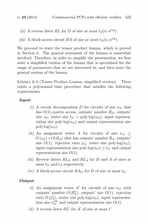
cc 23 (2014) Combinatorial PCPs with efficient verifiers 423
(ii) A reverse lister RL for D of size at most tD(n, nrep).
(iii) A block-access circuit BA of size at most tD(n, nrep).
We proceed to state the tensor product lemma, which is provedin Section 8. The general statement of the lemma is somewhatinvolved. Therefore, in order to simplify the presentation, we firststate a simplified version of the lemma that is specialized for therange of parameters that we are interested in, and then state thegeneral version of the lemma.
Lemma 6.4 (Tensor Product Lemma, simplified version). Thereexists a polynomial time procedure that satisfies the followingrequirements:
Input:
(i) A circuit decomposition D for circuits of size nD thathas O(1)-matrix access, outputs’ number RD, outputs’size sD, tester size tD = poly log(nD), input represen-tation size poly log(nD) and output representation sizepoly log(nD).
(ii) An assignment tester A for circuits of size nA ≥O (sD)+O(RD) that has outputs’ number RA, outputs’size O(1), rejection ratio ρA, tester size poly log(nD),input representation size poly log(nD) ≥ tD and outputrepresentation size O(1).
(iii) Reverse listers RLD and RLA for D and A of sizes atmost tD and tA respectively.
(iv) A block-access circuit BAD for D of size at most tD.
Output:
(i) An assignment tester A′ for circuits of size nD withoutputs’ number O(R2
A), outputs’ size O(1), rejectionratio Ω (ρ2
A), tester size poly log(nD), input representa-tion size nrep
D and output representation size O(1).
(ii) A reverse lister RL′ for A′ of size at most t′.
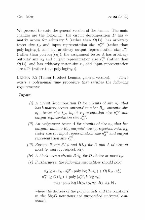
424 Meir cc 23 (2014)
We proceed to state the general version of the lemma. The mainchanges are the following: the circuit decomposition D has b-matrix access for arbitrary b (rather than O(1)), has arbitrarytester size tD and input representation size nrep
D (rather thanpoly log(nD)), and has arbitrary output representation size srep
D
(rather than poly log(sD)); the assignment tester A has arbitraryoutputs’ size sA and output representation size srep
A (rather thanO(1)), and has arbitrary tester size tA and input representationsize nrep
A (rather than poly log(nD)).
Lemma 6.5 (Tensor Product Lemma, general version). Thereexists a polynomial time procedure that satisfies the followingrequirements:
Input:
(i) A circuit decomposition D for circuits of size nD thathas b-matrix access, outputs’ number RD, outputs’ sizesD, tester size tD, input representation size nrep
D andoutput representation size srep
D .
(ii) An assignment tester A for circuits of size nA that hasoutputs’ numberRA, outputs’ size sA, rejection ratio ρA,tester size tA, input representation size nrep
A and outputrepresentation size srep
A .
(iii) Reverse listers RLD and RLA for D and A of sizes atmost tD and tA, respectively.
(iv) A block-access circuit BAD for D of size at most tD.
(v) Furthermore, the following inequalities should hold:
nA ≥ b · sD · srepD · poly log (b, sD) +O(RD · s2
A)
nrepA ≥ O (tD) + poly (srep
D , b, log sD)
+sA · poly log (RD, sD, nD, RA, sA, b) ,
where the degrees of the polynomials and the constantsin the big-O notations are unspecified universal con-stants.
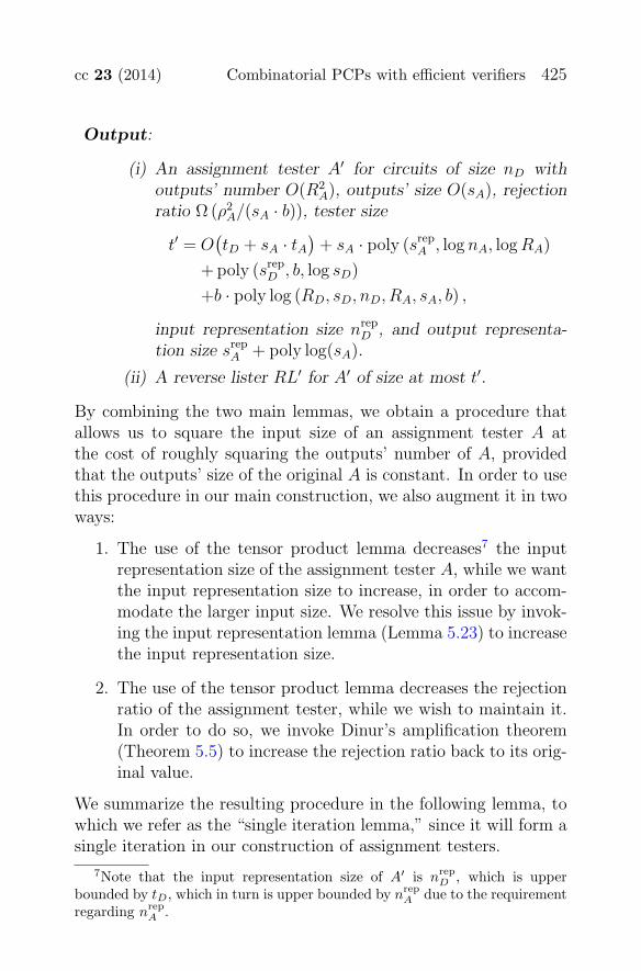
cc 23 (2014) Combinatorial PCPs with efficient verifiers 425
Output:
(i) An assignment tester A′ for circuits of size nD withoutputs’ number O(R2
A), outputs’ size O(sA), rejectionratio Ω (ρ2
A/(sA · b)), tester size
t′ = O(tD + sA · tA
)+ sA · poly (srep
A , log nA, logRA)
+ poly (srepD , b, log sD)
+b · poly log (RD, sD, nD, RA, sA, b) ,
input representation size nrepD , and output representa-
tion size srepA + poly log(sA).
(ii) A reverse lister RL′ for A′ of size at most t′.
By combining the two main lemmas, we obtain a procedure thatallows us to square the input size of an assignment tester A atthe cost of roughly squaring the outputs’ number of A, providedthat the outputs’ size of the original A is constant. In order to usethis procedure in our main construction, we also augment it in twoways:
1. The use of the tensor product lemma decreases7 the inputrepresentation size of the assignment tester A, while we wantthe input representation size to increase, in order to accom-modate the larger input size. We resolve this issue by invok-ing the input representation lemma (Lemma 5.23) to increasethe input representation size.
2. The use of the tensor product lemma decreases the rejectionratio of the assignment tester, while we wish to maintain it.In order to do so, we invoke Dinur’s amplification theorem(Theorem 5.5) to increase the rejection ratio back to its orig-inal value.
We summarize the resulting procedure in the following lemma, towhich we refer as the “single iteration lemma,” since it will form asingle iteration in our construction of assignment testers.
7Note that the input representation size of A′ is nrepD , which is upper
bounded by tD, which in turn is upper bounded by nrepA due to the requirement
regarding nrepA .
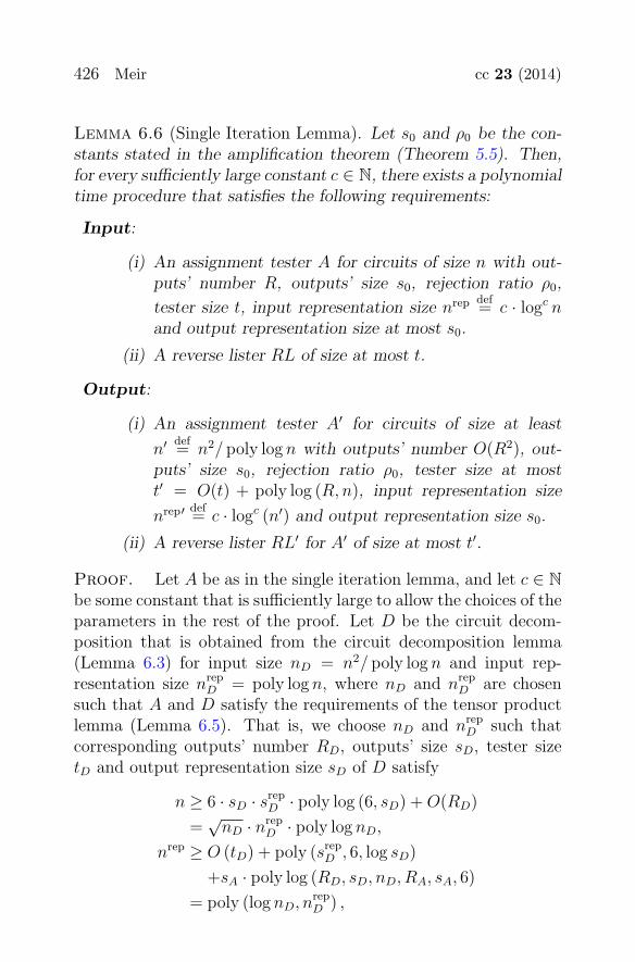
426 Meir cc 23 (2014)
Lemma 6.6 (Single Iteration Lemma). Let s0 and ρ0 be the con-stants stated in the amplification theorem (Theorem 5.5). Then,for every sufficiently large constant c ∈ N, there exists a polynomialtime procedure that satisfies the following requirements:
Input:
(i) An assignment tester A for circuits of size n with out-puts’ number R, outputs’ size s0, rejection ratio ρ0,
tester size t, input representation size nrep def= c · logc n
and output representation size at most s0.
(ii) A reverse lister RL of size at most t.
Output:
(i) An assignment tester A′ for circuits of size at least
n′ def= n2/ poly log n with outputs’ number O(R2), out-
puts’ size s0, rejection ratio ρ0, tester size at mostt′ = O(t) + poly log (R, n), input representation size
nrep′ def= c · logc (n′) and output representation size s0.
(ii) A reverse lister RL′ for A′ of size at most t′.
Proof. Let A be as in the single iteration lemma, and let c ∈ N
be some constant that is sufficiently large to allow the choices of theparameters in the rest of the proof. Let D be the circuit decom-position that is obtained from the circuit decomposition lemma(Lemma 6.3) for input size nD = n2/ poly log n and input rep-resentation size nrep
D = poly log n, where nD and nrepD are chosen
such that A and D satisfy the requirements of the tensor productlemma (Lemma 6.5). That is, we choose nD and nrep
D such thatcorresponding outputs’ number RD, outputs’ size sD, tester sizetD and output representation size sD of D satisfy
n ≥ 6 · sD · srepD · poly log (6, sD) +O(RD)
=√nD · nrep
D · poly log nD,
nrep ≥ O (tD) + poly (srepD , 6, log sD)
+sA · poly log (RD, sD, nD, RA, sA, 6)
= poly (log nD, nrepD ) ,
cc 23 (2014) Combinatorial PCPs with efficient verifiers 427
where the hidden constants are determined by the decompositionand the tensor product lemma. It can be verified that for suf-ficiently large choice of the constant c, one can indeed choosenrep
D = poly log n in a way that satisfies the above inequalities.We note that the decomposition D has outputs’ number O (n),
outputs’ size O (n), tester size tDdef= poly log (n), input representa-
tion size nrepD and output representation size poly log (n), and that
D is 6-matrix based. We also obtain from the circuit decomposi-tion lemma a reverse lister RLD for D and a block access circuitBAD for D, both of size at most tD.
We now invoke the tensor product lemma on D and A, result-ing in an assignment tester A1 for circuits of size nD with out-
puts’ number R1def= O(R2), outputs’ size s0, rejection ratio ρ1
def=
Ω (ρ20/(s0 · 6)) = Ω(1), tester size
t1def= O (tD + s0 · t) + s0 · poly (s0, log n, logR)
+ poly (srepD , 6, log sD) + 6 · poly log (RD, sD, nD, R, s0, 6) ,
= O(t) + poly log (n,R) ,
input representation size nrepD and output representation size s0.
We also obtain a reverse lister RL1 for A1 of size at most t1.Next, we apply the input representation lemma (Lemma 5.23)
to A1, with input representation size nrep′ def= c · logc(n2). We
therefore obtain an assignment tester A2 for circuits of size
n′ def= nD/n
rep′ · poly log nD = n2/ poly log(n)
that has outputs’ number R2 = O(R1) = O(R2), outputs’ size
s2 = max {s0, O(1)}, rejection ratio ρ2def= Ω(ρ1) = Ω(1), tester size
t2def= O(t1) + poly
(nrep′, log n
)= O(t) + poly log (n,R) ,
input representation size nrep′ ≥ c · logc(n′) and output represen-tation size max {s0, O(1)}. We also obtain a reverse lister RL2
for A2 of size at most t2. We mention that in order for us tobe able to apply the input representation lemma, we need nrep
D tobe sufficiently large. However, for sufficiently large choice of the
428 Meir cc 23 (2014)
constant c, it is possible to choose nrepD in a way such that the
conditions of both the tensor product lemma and the input repre-sentation lemma are met.
Finally, we apply the amplification theorem (Theorem 5.5) toA2, resulting in an assignment tester A′ for circuits of size n′ withoutputs’ number poly
(s0,
1ρ2
) ·R2 = O(R2), outputs’ size s0, rejec-tion ratio ρ0, tester size
t′ def= poly
(s0,
1
ρ2
) · (t2 + poly (s0) + poly log (R2, n′))
= O(t) + poly log (n,R) ,
input representation size nrep′ and output representation size s0.We also obtain a reverse lister RL′ for A′ of size at most t′. We nowoutput A′ and RL′ as the required assignment tester and reverselister. �
We finally turn to prove our main theorem, restated below, bystarting from an assignment tester for circuits of constant size,and applying the single iteration lemma for O(log log n) times.
Theorem (4.9, Main Theorem). There exists an infinite family ofcircuits {An,nrep}∞
n=1,nrep=1, such that An,nrep is an assignment testerfor circuits of size n with outputs’ number R(n) = poly (n), out-puts’ size s(n) = O(1), proof length � (n) = poly (n), rejection ratioρ = Ω(1), tester size t(n, nrep) = poly (log n, nrep), input represen-tation size nrep and output representation size srep(n, nrep) = O(1).Furthermore, there exists an algorithm that on inputs n and nrep,runs in time poly (log n, nrep) and outputs An,nrep .
Proof. Let c be a constant that will be determined later. Wewill choose c to be sufficiently large to match the requirements ofthe single iteration lemma (Lemma 6.6). We first show how toconstruct assignment testers An,nrep for nrep = c · logc n by iter-ative application of the single iteration lemma (Lemma 6.6) andthen use the input representation lemma (Lemma 5.23) to obtainassignment testers for any desired input representation size. Wealso mention that in the following proof, we do not prove that theproof length is poly(n), but as in the rest of this paper, this can be
cc 23 (2014) Combinatorial PCPs with efficient verifiers 429
established using the upper bound � ≤ R ·s (Theorem 5.4). Detailsfollow.
Let n ∈ N and let nrep = c · logc n. Let s0 and ρ0 be as in thesingle iteration lemma. We construct an assignment tester An,nrep
as in the theorem as follows. We begin by constructing an assign-ment tester A0 for circuits of size n0, where n0 is some sufficientlylarge constant that is independent of n. We construct A0 such thatit has outputs’ size s0, rejection ratio ρ0, input representation size
nrep0
def= c · logc n0 and output representation size s0, and such that
its outputs’ number R0 and tester size t0 are constants indepen-dent of n. Such an assignment tester A0 can be constructed, forexample, by using the circuit decomposition lemma (Lemma 6.3)to generate a circuit decomposition D with input size n0 and inputrepresentation size nrep
0 , and then invoking the amplification the-orem (Theorem 5.5) to D in order to yield A0. This also yields areverse lister RL0 for A0.
Now, for each natural number i ≥ 1, we let Ai and RLi be theassignment tester and reverse lister that are obtained by invokingthe single iteration lemma on the assignment tester Ai−1 and onthe reverse lister RLi−1. We denote by ni the input size of Ai, byRi the outputs’ number of Ai and by ti the tester size of Ai. Letk be the least natural number such that nk ≥ n. We output Ak asour desired assignment tester An,nrep .
We turn to analyze the parameters of Ak and start with findingan upper bound on k. By the single iteration lemma, there existsa constant d such that for every i, it holds that ni+1 = n2
i /d ·logd n. In Appendix A, we show that for every i, it holds that
ni ≥ (n0/d · 2d · logd n0
)2i
. Hence, by taking n0 to be sufficiently
large such that n0/d · 2d · logd n0 > 1, we get that
k ≤ log2 log(n0/d·2d·logd n0) n = log log n−O(1).
It is not hard to see that Ak has outputs’ size s0, rejectionratio ρ0, input representation size at least c · logc n and outputrepresentation size s0. We proceed to analyze the outputs’ numberand tester size of Ak. By the single iteration lemma, there existssome constant hR such that for each i ≥ 1, it holds that Ri ≤
430 Meir cc 23 (2014)
hR · (Ri−1)2. It is not hard to prove by induction that
Ri = h∑i−1
j=0 2j
R R2i
0 ≤ (hR ·R0)2i
,
and therefore
Rk ≤ (hR ·R0)2k ≤ (hR ·R0)
log n ≤ poly(n).
In addition, by the single iteration lemma, there exists some con-stant ht such that for each i ≥ 1, it holds that ti ≤ ht ·t+poly log n,and therefore
tk ≤ hkt · t0 + k · hk
t · poly log n ≤ poly log n,
as required. Finally, observe that it is possible to compute Ak intime poly log n.
We now consider the case of general values of nrep. Letn, nrep ∈ N. We construct the assignment tester An,nrep as follows.We first observe that we may assume without loss of generalitythat nrep ≤ poly(n), since every circuit of size n has a trivial rep-resentation of size poly(n). Let n′ = n · nrep · poly log n, and letnrep′ = c · logc (n′). We construct the assignment tester An′,nrep′ andinvoke the input representation lemma (Lemma 5.23) on An′,nrep′
to increase its input representation size to nrep. We then outputthe resulting assignment tester as An,nrep . It is not hard to checkthat An,nrep has the required parameters, and that the latter invo-cation of the input representation lemma is indeed legal, since theassignment tester An′,nrep′ indeed satisfies the requirements of theinput representation lemma for sufficiently large choice of c. �
7. Circuit decomposition lemma
In this section, we prove the circuit decomposition lemma, restatedbelow.
Lemma (6.3, Circuit decomposition lemma, restated). Thereexists a procedure that when given as inputs numbers n, nrep ∈ N,runs in time poly (log n, nrep) and outputs the following:
cc 23 (2014) Combinatorial PCPs with efficient verifiers 431
(i) A circuit decomposition D for circuits of size n that has 6-
matrix access, outputs’ number RD(n)def= O(
√n), outputs’
size sD(n)def= O(
√n), tester size tD(n, nrep)
def= poly log n +
O(nrep), input representation size nrep, and output represen-
tation size srepD (n, nrep)
def= poly log n+O(nrep).
(ii) A reverse lister RL for D of size at most tD(n, nrep).
(iii) A block-access circuit BA of size at most tD(n, nrep).
In Section 7.1, we give an overview of the proof, which is moredetailed than the one given in Section 3.2. Then, in Section 7.2,we provide the full proof of the lemma.
Bounding the fan-in and fan-out of circuits. In this section,we describe the construction of a circuit decomposition D thatcan only handle input circuits whose fan-in and fan-out are upperbounded by 2. However, such a decomposition can be transformedinto a full-fledged decomposition, which can deal with arbitraryfan-in and fan-out, by using the fan-in/out lemma (Lemma 5.27).
7.1. Overview. In this section, we give an overview of the con-struction of the circuit decomposition D from the decompositionlemma. In order to streamline the presentation, we describe D bydescribing its action on a fixed input circuit ϕ of size n over minputs, on a fixed assignment x ∈ {0, 1}m and on a fixed proofstring π. As we mentioned above, the fan-in and fan-out of ϕ areassumed to be upper bounded by 2. Furthermore, recall that wewant D to have 6-matrix access, which essentially means that:
1. The assignment x and proof string π should be arranged intwo matrices, namely the assignment matrix and the proofmatrix.
2. Every output circuit of D should query 6 rows of theassignment and proof matrices. Actually, in this simplifiedoverview, the output circuits of D will query even less than 6rows of the matrices.
432 Meir cc 23 (2014)
This overview is divided to two parts. First, in Section 7.1.1, wedescribe a construction of D while ignoring efficiency considera-tions, which yields a decomposition D that is not super-fast. Then,in Section 7.1.2, we describe how to modify D into a super-fastdecomposition.
7.1.1. Warm-up: ignoring efficiency considerations.
The basic idea. The basic structure of our construction of thedecomposition D goes as follows. We require the proof string π tocontain the following values:
◦ The value that each gate g of ϕ outputs when ϕ is invokedon x. Let us denote by kg the coordinate of π that containsthe value of g.
◦ The value that each wire (g1, g2) of ϕ carries when ϕ isinvoked on x. Let us denote by k(g1,g2) the coordinate ofπ that contains the value of (g1, g2).
Then, the output circuits of D should check the following condi-tions hold:
1. For every input gate g, it holds that πkg equals to the corre-sponding assignment coordinate.
2. For the output gate gout of ϕ, it holds that πkgout= 1.
3. For every gate g and its outgoing wires (g, g1) and (g, g2), itholds that πkg = πk(g,g1)
= πk(g,g2).
4. For every gate g and its incoming wires (g1, g) and (g2, g), itholds that πkg is indeed the value that g outputs when givenas input πk(g,g1)
and πk(g,g2).
The nontrivial issue, of course, is to arrange the proof string π ina O(
√n) × O(
√n) matrix such that the output circuits of D can
verify the foregoing conditions and such that every output circuitqueries only 6 rows of the matrix. Observe that arranging π insuch a matrix would have been easy if we only wanted to verifyonly one of the Conditions 3 and 4:
cc 23 (2014) Combinatorial PCPs with efficient verifiers 433
◦ If we only wanted to verify the Condition 3, we could arrangeπ in a matrix such that for each a gate g and its outgoingwires (g, g1) and (g, g2), the coordinates kg, k(g,g1), and k(g,g2)
are in the same row. Using this arrangement, Conditions 3, 1,and 2 could be verified with each output circuit ofD queryingonly one row of the matrix.
◦ On the other hand, if we only wanted to verify the Condi-tion 4, we could arrange π in a matrix such that for each agate g and its incoming wires (g1, g) and (g2, g), the coordi-nates kg, k(g1,g), and k(g2,g) are in the same row. Using thisarrangement, Conditions 4, 1, and 2 could be verified witheach output circuit of D querying only one row of the matrix.
The problem is that we do not know whether there is a singlearrangement of π in a matrix that allows verifying both conditionssimultaneously. Our first step toward solving the problem is torequire π to contain two matrices M and N , such that each of Mand N contains a copy of the value of each gate and each wire, andsuch that M is a arranged in the way that allows verifying Condi-tion 3 (as described above), and N is arranged in a way that allowsverifying Condition 4 (as described above). More specifically,
◦ For each gate g, the proof string π has a coordinate kM,g of thematrix M , and a coordinate kN,g of the matrix N where bothcoordinates should contain the value that g outputs when ϕis invoked on the assignment x. The matrices M and N alsohave similar coordinates kM,(g1,g2) and kN,(g1,g2) for each wire(g1, g2).
◦ For each a gate g and its outgoing wires (g, g1) and (g, g2),the coordinates kM,g, kM,(g,g1), and kM,(g,g2) are in the samerow of M . Similarly, for each a gate g and its incoming wires(g1, g) and (g2, g), the coordinates kN,g, kN,(g1,g), and kN,(g2,g)
are in the same row of N .
This way, the output circuits of D can verify that M satisfies Con-dition 3 and that N satisfies Condition 4, while each output cir-cuit queries only one row of those matrices. By concatenating the
434 Meir cc 23 (2014)
matrices M and N into a single matrix, we arrange π in a sin-gle matrix such that the two conditions can be verified while eachoutput circuit queries only one row of this matrix.
Of course, in order for the foregoing construction of D to besound, we also need to verify that M and N are consistent. Thatis, in addition to verifying the above conditions, the decompositionD must also verify that for each gate g and wire (g1, g2), it holdsthat
(7.1) πkM,g= πkN,g
and πkM,(g1,g2)= πkN,(g1,g2)
.
Moreover, D must verify that Equality 7.1 holds while maintainingthe property that each output circuit queries at most 6 rows of theproof matrix. Overcoming this issue of verifying the consistencyof M and N while maintaining the matrix access property is themain technical challenge that we deal with in our constructionof D.
Verifying the consistency of M and N . We now describehow D checks the consistency of the matrices M and N . As awarm-up, consider the following naive solution: For each row of M ,the decomposition D will output a circuit ψi that will check theconsistency of the coordinates in this row with the correspondingcoordinates in N . This solution does not work, since some of thoseoutput circuits ψi may read too many rows of N . To see it, observethat for the coordinates of a given row of M , the correspondingcoordinates in N may spread over all the rows of N rather thanbeing concentrated in only 5 rows of N .
On a more intuitive level, the latter naive solution does not workbecause the order of the coordinates in M may be very differentthan the order of the corresponding coordinates in N . Our solutionis to add to the proof matrix auxiliary rows that serve as a “bridge”between M and N , and to add output circuits of D that checkthe consistency of those auxiliary rows. More specifically, we addauxiliary rows and output circuits such that:
◦ Each auxiliary row v consists of coordinates kv,g and kv,(g1,g2)
that correspond to some of the gates and wires of ϕ. As
cc 23 (2014) Combinatorial PCPs with efficient verifiers 435
before, πkv,g is supposed to contain the value that the gate goutputs when ϕ is invoked on x, and πkv,(g1,g2)
is supposedto contain the value that the wire (g1, g2) carries when ϕ isinvoked on x. However, note that each auxiliary row is ofwidth O(
√n), so it does not contain a coordinate for every
gate and wire.
◦ For each auxiliary row v, there will be an output circuit of Dthat checks the consistency of the row v with at most fourother rows of the proof matrix. By saying that an outputcircuit ψi checks the consistency of two rows u and v, we meanthat ψi checks, for every two coordinates ku,g and kv,g of uand v that correspond to the same gate g, that πku,g = πkv,g ,and the same for the wires.
◦ We will choose the auxiliary rows and additional output cir-cuits such that all the additional output circuits are satisfiedif and only if M and N are consistent.
It remains to explain how to choose for each auxiliary row v:
◦ For which gates g and wires (g1, g2) does the auxiliary row vhave corresponding coordinates kv,g and kv,(g1,g2)?
◦ What are the other rows of the proof matrix with which theauxiliary row v is checked for consistency.
To this end, we use routing networks. Recall that a routing networkof order n is a graph with two special sets S and T , called the“sources” and the “targets,” and that a routing network satisfiesthe following property: Suppose that for every source s ∈ S, thereare d messages that should be sent to targets in T , and that everytarget t ∈ T should receive d messages from sources in S. Then, itis possible to find a collection of paths P in G such that:
◦ Every message is routed through some path p ∈ P. We saythat the path p routes the message if its connects the sourceof the message to its target.
◦ Every vertex of G participates in at most d paths in P.
436 Meir cc 23 (2014)
Let G = (V,E) be a routing network of order O(√n) with in-degree
and out-degree upper bounded by 2, and let S and T be its sourcesand targets, respectively. We identify the vertices of G with therows of the proof matrix, and in particular, we identify the rowsof M with the vertices of S, the rows of N with the vertices of Tand the auxiliary rows of the proof matrix with the other verticesof G.
Now, for each gate g, we view the value that g outputs (underthe assignment x) as a message that should be sent from the rowof M that contains the coordinate kM,g to the row of N that con-tains the coordinate kN,g, where we view those rows of M and Nas a source and a target of G. We also view the values of wires(g1, g2) as messages in a similar way. Note that, when taking thisview, each row of M needs to send O(
√n) messages and each row
of N needs to receive O(√n) messages.
Our next step is to find a collection of paths P along which themessages can be routed, such that each auxiliary row participatesin the routing of at most O(
√n) messages (i.e., the vertex of G that
is identified with the auxiliary row participates in at most O(√n)
paths in P). For each auxiliary row v and a gate g, we definethe auxiliary row v to contain a coordinate kv,g that correspondsto g if and only if the auxiliary row v participates in routing themessage that corresponds to the value of g, and the same goes foreach wire (g1, g2).
Finally, we define the output circuits of D that verify the con-sistency of the auxiliary rows as follows. For each vertex v of G,the decomposition outputs a circuit ψi that acts as follows. Sup-pose that v has outgoing edges to the vertices z1 and z2 of G(recall that the out-degree of G is upper bounded by 2). Then,the circuit ψi queries the rows that correspond to v, z1 and z2, andperforms the following consistency check. For every gate g whosecorresponding message is routed through v, the circuit ψi verifiesthat πkv,g = πkz1,g if the message of g is routed through z1, andotherwise ψi verifies that πkv,g = πkz2,g (since if the message is notrouted through z1, then it must be routed through z2). The cir-cuit ψi also performs an analogous consistency check for every wire(g1, g2) whose corresponding message is routed through v.
cc 23 (2014) Combinatorial PCPs with efficient verifiers 437
This concludes the description of our way of verifying the con-sistency of M and N , and in particular our construction of theauxiliary rows and the output circuits of D. It is not hard to seethat if all the output circuits of D accept, then M and N mustbe consistent. Observe that every output circuit queries at mostthree rows. Moreover, note that every auxiliary row contains atmost O(
√n) coordinates, since it participates in the routing of at
most O(√n) messages.
The assignment matrix. Our discussion so far has focused onthe proof string π and the arrangement of its coordinates in theproof matrix. However, we still need to describe the arrangementof the assignment x in the assignment matrix. For convenience,let us denote the assignment matrix by L. We choose L to be ofwidth wa = min {θ(√n),m} and arrange the coordinates of x in Laccording to their natural order.
Another issue that we ignored so far is that the decomposi-tionD should check the consistency between the assignment matrixand the proof matrix. More formally, for every tested assignmentcoordinate ka ∈ [m] whose corresponding input gate of ϕ is g, thedecomposition D should check that xka = πkM,g
. To this end, wechoose the ordering of the coordinates of the matrix M such thatthe assignment coordinate ka is in the j-th row of L if and only ifthe corresponding proof coordinate kM,g belongs to the j-th row ofM . Then, for each j, the decomposition D outputs a circuit thatchecks that all the coordinates in the j-th row of L are consistentwith the corresponding coordinates in the j-th row of M .
Conclusion. It can be seen that x is a satisfying assignment ifand only if there exists a proof string π that makes all the outputcircuits ψi accept. Moreover, observe that the number and size ofoutput circuits of D is indeed O(
√n), and that each output circuit
queries at most three rows of the assignment and proof matrices.This concludes our construction of D that ignores the efficiencyissues.
Remark 7.2. We mention again that the idea of using routingnetworks in the construction of PCPs is not new and already
438 Meir cc 23 (2014)
appeared in several works on PCPs (see, e.g., Babai et al. 1991a;Polishchuk & Spielman 1994).
7.1.2. Obtaining a super-fast circuit decomposition. Weturn to explain how to modify the foregoing circuit decomposi-tion such that it will have a super-fast implementation. The mainissue that needs to be resolved is the following: Recall that thedecomposition routes messages on the routing network G. Morespecifically, the decomposition computes a collection P of paths onG that connect each coordinate of M to its corresponding coordi-nate of N , where each vertex in G participates in at most O(
√n)
such paths. However, those paths cannot be computed by asuper-fast decomposition, since merely writing those paths downrequires writing Ω(n) bits, which would force the decompositionto be of size Ω(n) rather than poly log n. In order to resolve thisissue, we modify the decomposition such that it does not com-pute those paths by itself. Instead, we require the proof stringto contain those paths and modify the decomposition such thatit verifies that the paths that are given in the proof string arevalid.
This idea is implemented as follows: For each coordinate kv,g
in the proof string, we add to the row of kv,g additional log n coor-dinates that are supposed to be assigned the index of g—we referto this index as the label of kv,g. Similarly, for each coordinatekv,(g1,g2), we add to the row of kv,(g1,g2) additional 2 log n coordi-nates that are supposed to contain the indices of g1 and g2, andrefer to the pair of those indices as the label of kv,(g1,g2). We notethat this modification is also performed on rows of M and N .
Now, we modify the output circuits ψi that verify the consis-tency of the routing as follows. Let ψi be the output circuit thatcorresponds to a vertex v, and suppose that v has incoming edgesfrom the vertices u1 and u2, and has outgoing edges to the verticesz1 and z2. Then, the output circuit ψi reads the rows that corre-spond to u1, u2, v, z1, z2, and verifies that the following conditionsholds:
1. Every label in the row of v is found either in the row of u1
or in the row of u2.
cc 23 (2014) Combinatorial PCPs with efficient verifiers 439
2. Every label in the row of v is found either in the row of z1 orin the row of z2.
3. If a coordinate k in the row of v has the same label as acoordinate k′ in the row of u1, then πk = πk′ . The samecondition is checked when replacing u1 with either of u2, z1,or z2.
It can be seen that if all the modified output circuits ψi accept,then we are guaranteed that the matrices M and N are consistent.In addition to modifying the output circuits as above, we also addnew output circuits ψi that check that the coordinates of M andN have the correct labels, and in particular that:
◦ Every gate and every wire have corresponding coordinates inM and in N .
◦ For each a gate g and its outgoing wires (g, g1) and (g, g2),the coordinates kM,g, kM,(g,g1), and kM,(g,g2) are in the samerow of M .
◦ For each a gate g and its incoming wires (g1, g) and (g2, g),the coordinates kN,g, kN,(g1,g), and kN,(g2,g) are in the samerow of N .
Note that in the super-fast setting, in which the gate or wire towhich a coordinate corresponds is determined by its label, the lat-ter three conditions must indeed be verified and cannot be assumedto hold trivially as before. However, it is not hard to construct out-put circuits of D that verify those conditions.
It is not hard to see that the decomposition D remains soundafter the foregoing modifications. Moreover, since now D needsnot compute the paths P for routing the messages, it can be imple-mented in a super-fast way. This concludes the construction.
7.2. Proof of the circuit decomposition lemma. Below, wedescribe how to construct the circuit decomposition D for a giveninput size n and a given input representation size nrep. This sectionis organized as follows: In Section 7.2.1, we describe the blockstructure of D. In Section 7.2.2, we describe the proof strings of
440 Meir cc 23 (2014)
D. In Section 7.2.3, we describe the output circuits of D and theirqueries. The remaining parts of the proof, namely the constructionof the reverse lister RLD, the construction of the blocks accesscircuitBAD and the analysis of the parameters, are straightforwardand will not be discussed.
7.2.1. The block structure of D.
The assignment blocks. Let wa be the width of the assign-ment blocks, to be chosen shortly below. We define the assignmentblocks of D on input circuit ϕ as follows: There are �m/wa� assign-ment blocks, where the first assignment block consists of the coor-dinates 1, . . . , wa, the second assignment block consists of the coor-dinates wa+1, . . . , 2·wa, etc. If wa does not divide m, then the lastassignment block consists of the last m mod wa assignment coor-dinates and of additional wa − (m mod wa) dummy coordinates.
We now choose wa = min {θ(√n),m}, where the constant inthe Big-Theta notation is chosen as follows: Recall that the defi-nition of block access requires that least 1
3fraction of the coordi-
nates of every assignment block are nondummy coordinates. Theonly assignment block that contains dummy coordinates is the lastblock, so we only need to take care of this block. To this end, weneed to choose wa such that if wa < m, then (m mod wa) ≥ 1
3·wa.
It is not hard to show that one can choose such a value of wa thatsatisfies wa = min {θ(√n),m}, as required.
The proof blocks. We turn to define the proof blocks of D. Let
wrdef= 3 · max {√
n,wa}.We denote by wπ the width of the proof
blocks and choose it to be wπdef= wr · (2 · log n+ 3). The first proof
block of D consists of the coordinates m+1, . . . ,m+wπ, the secondproof block of D consists of the coordinates m + wπ + 1, . . . ,m +2 ·wπ, etc. We view each proof block as consisting of 3 ·wr stringsof length 2 · log n+ 1, to which we refer as the records of the blockand view each record of consisting of two parts:
1. The label of the record, which consists of two elements in[n] ∪ {⊥}—this part is represented by the first 2 · (log n+ 1)bits of the record.
cc 23 (2014) Combinatorial PCPs with efficient verifiers 441
2. The value of the record, which is a Boolean value, and isrepresented by the last bit of the record.
Let Gdef= G√
n be the routing network of order√n whose existence
is guaranteed by Fact 2.16, and let S and T be its sets of sourcesand targets, respectively. We define the proof blocks of D to bein one-to-one correspondence with the vertices of G, where the j-th proof block corresponds to the j-th vertex of G. We view the√n proof blocks which correspond to the vertices in S of G as an√n×wπ matrix M , and the
√n proof blocks which correspond to
vertices in T as an√n× wπ matrix N .
7.2.2. The proof strings of D. Let x be a satisfying assign-ment for ϕ. We describe the proof string π that convinces D that xsatisfies ϕ. We consider the collection of all the records in all of theblocks and view each record as corresponding to a gate or a wireof ϕ, where each gate (or wire) has many records that correspondto it. The content of π at a given record depends on whether therecord corresponds to a gate or to a wire, and is determined asfollows:
1. If the record corresponds to a gate g, then the first elementof the label of the record contains the index of g (which isa number from 1 to n), and the second element of the labelcontains the symbol ⊥. The value of the record is set to be thevalue that g outputs when ϕ is invoked on the assignment x.
2. If the record corresponds to a wire (g1, g2), then first elementof the label of the record contains the index of g1 and thesecond element is of the label contains the index of g2 (recallthat those indices are numbers from 1 to n). The value of therecord is set to be the value that is passed through (g1, g2)when ϕ is invoked on the assignment x.
3. Finally, some records are dummy records that do not corre-spond to a gate or a wire of ϕ. In this case, both elements ofthe label of the record contain the symbol ⊥, and the valueof the record is arbitrary.
442 Meir cc 23 (2014)
It remains to describe the correspondence between records andgates/wires—note that since the content of a record is determinedby the gate/wire to which it corresponds, this correspondencedetermines π completely. We describe this correspondence sep-arately for the matrix M , the matrix N and the rest of the proofblocks.
The matrix M . There is a one-to-one correspondence betweenthe records in M and the gates and wires of ϕ. If there are morerecords than gates and wires, then the superfluous records are setto be dummy records.The order of the records in M is as follows: Each row of M consistsof wr/3 triplets of records, where each such triplet corresponds to agate g of ϕ and is referred to as the triplet of g in M . Given a gate g,the triplet of g contains the record that corresponds to g and alsothe records that correspond to the (at most two) outgoing wiresof g. If g has less than two outgoing wires, then the (one or two)superfluous records are set to be dummy records, which containonly zeroes. The triplets are ordered in M according to the orderof the gates, from the first gate to the last.
The matrix N . The records of N are defined similarly to therecords of M , with the following differences. For each gate g, thetriplet of g inN contains the records corresponding to the incomingwires of g rather than the outgoing wires of g.
The auxiliary rows. Recall that each proof block correspondsto some vertex of the routing network G, where the matrices Mand N correspond to the sources set S and targets set T of G. Thecorrespondence of records to gates and wires in the auxiliary rowswill be determined by routing on G, which will be performed usingProposition 2.17, restated below.
Proposition (2.17, routing of multiple messages, restated). LetG = (V,E) be a routing network of order n, let S, T ⊆ V bethe sets of sources and targets of G, respectively, and let d ∈ N.Let σ ⊆ S×T be a relation such that each s ∈ S is the first element
cc 23 (2014) Combinatorial PCPs with efficient verifiers 443
of at most d pairs in σ, and such that each t ∈ T is the secondelement of at most d pairs in σ. We allow σ to be a multiset, i.e.,to contain the same element multiple times. Then, there exists aset P of paths in G such that the following holds:
(i) For each (s, t) ∈ σ, there exists a path p ∈ P that correspondsto (s, t), whose first vertex is s and whose second vertex in t.
(ii) Every vertex of G participates in at most d paths in P.
We turn to describe the routing. We construct a relation σ ⊆ S×T(actually, a multiset) as follows: For each gate g of ϕ, we add σthe pair (s, t), where
1. s ∈ S is the vertex of G that corresponds to the row of Mthat contains the record of g in M .
2. t ∈ T is the vertex of G that corresponds to the row of Nthat contains the record of g in N .
We do the same for the wires of ϕ. Now, by Proposition 2.17, thereexists a collection P of paths such that
1. For each (s, t) ∈ σ, there exists a path p ∈ P that correspondsto (s, t), whose first vertex is s and whose second vertex in t.
2. Every vertex of G participates in at most wr paths in P.
We now define the records of the auxiliary rows. For each gate g,we define the following records: let (s, t) be the element of σ thatcorresponds to g, and let p ∈ P be the path that corresponds to(s, t). Now, for each vertex v on the path p, the auxiliary row vcontains a record that corresponds to g. The same goes for eachwire (g1, g2) and the corresponding element (s, t) and path p. If avertex v of G participates in less than wr paths, then the remainingrecords of the auxiliary row v are set to be dummy records.
This concludes the description of the correspondence betweenthe records and the gates/wires, and hence concludes the descrip-tion of the proof string π.
444 Meir cc 23 (2014)
7.2.3. The output circuits of D . In this section, we describethe output circuits of the circuit decompositionD and their queries.Fix an input circuit ϕ of size n and overm inputs. Let V denote thevertex set of the routing networkG. We define the outputs’ numberRD of D to be |V |+2 ·√n. We view the first |V | output circuits asbeing in one-to-one correspondence with the vertices of G, the next√n output circuits as being in one-to-one correspondence with the
rows of M and the last√n output circuits as being in one-to-one
correspondence with the rows of N .We describe for each index i ∈ [RD] what the i-th output circuit
checks and what blocks it queries. We consider the following cases:
1. i ≤ |V |: In such case, the i-th output circuit ψi correspondsto some vertex v of G, which in turn corresponds to the i-thproof block of D. The goal of the output circuit ψi is to checkthat the routing at the vertex v is valid—that is, that everyrecord that is routed through v has came through one of theincoming edges of v and is sent through one of the outgoingedges of v. To this end, the output circuit ψi queries theblocks that correspond to v and its neighbors, and performsthe following checks:
(a) Let u1, . . . , ud (for d ≤ 2) be the vertices of G fromwhich v has incoming edges (if v has no incoming edges,then this check is skipped). Then, ψi checks for eachrecord of the i-th proof block that one of the blocksthat correspond to u1, . . . , ud contains a record with thesame label and the same value.
(b) The same check as the first one, but for vertices of Gto which v has outgoing edges, instead of vertices of Gfrom which v has incoming edges. Again, if v has nooutgoing edges, then this check is skipped.
We note that the output circuit ψi can be implemented in sizeO (
√n) as follows: For the first check, ψi constructs a list of
all the records that appear in the blocks that correspond tou1, . . . , ud, and sorts those records according to lexicographicorder of their label. Then, ψi sorts the records that appear
cc 23 (2014) Combinatorial PCPs with efficient verifiers 445
in the i-th block according to their label, thus obtaining asecond list of records. Finally, ψi checks that the secondlist of records is a subsequence of the first list of records.The second check can be implemented similarly. It can beverified that this implementation indeed requires a circuit ofsize O (
√n).
2. |V | + 1 ≤ i ≤ |V | +√n: Let j
def= i − |V |. In this case,
the output circuit ψi queries the j-th row of M and checksthat it is of the form described in Section 7.2.2. That is, ψi
checks that the j-th row of M consists of triplets of records,where each triplet consists of the record of a gate and of therecords of the gate’s outgoing wires, and where the values ofthe records of each triplet are equal. More specifically, forevery u ∈ [wr], the output circuit ψi performs the followingchecks for the u-th triplet of the j-th row:
(a) ψi computes the index hdef= (j − 1) · max {wa,
√n} + u
of the triplet among all the triplets of M . Let us denotethe h-th gate of ϕ by g.
(b) ψi checks that the first record of the triplet correspondsto g, that is, that the first element of the label of thefirst record contains h and that the second element con-tains ⊥.
(c) ψi checks that the labels of the two last records of thetriplet are the labels of the outgoing wires of the gate g.If g has only one outgoing wire, then g checks that thelabel of the middle record is the label of this unique out-going wire, and that the label of the last record consistsof twice the symbol ⊥. If g has no outgoing wires, theng checks that the labels of both the last records consistof twice the symbol ⊥.
(d) ψi checks that the values of all the three records in thetriplet are equal (recall that those values are supposedto be equal to the value that g outputs when ϕ is invokedon x).
446 Meir cc 23 (2014)
If j ≤ �m/wa�, then ψi also queries the j-th row of the assign-ment matrix and checks consistency between this row andthe records of M that correspond to input gates. Specifi-cally, observe that for each assignment coordinate in the j-throw of the assignment matrix, the record of the correspond-ing input gate is found in the j-th row of M . The outputcircuit ϕi checks for each such assignment coordinate that itis equal to the value of the corresponding record.
3. |V | +√n + 1 ≤ i ≤ |V | + 2 · √
n: Let jdef= i − |V | − √
n.In this case, the output circuit ψi queries the j-th row of Nand checks that it is of the form described in Section 7.2.2.That is, ψi checks that the j-th row of N consists of tripletsof records where each triplet consists of the record of a gateand of the records of its incoming wires, and where the valueof each gate record is computed correctly from the values ofthe records of the incoming wires. To this end, ψi performsthe same checks as in Case 2, with the following differences:
(a) Instead of checking for each triplet that the last tworecords contain the labels of the outgoing wires, ψi
checks that last two records contain the labels of theincoming wires.
(b) Instead of checking for each triplet that the values ofall the three records are the same, ϕi checks that thevalue of the first record, which corresponds to the gateg, contains the value that g outputs when g is given asinput the values of the two last records. If g has onlyone incoming wire, then we take only the value of themiddle record, and if g has not incoming wires, then thischeck is skipped.
(c) ψi does not check consistency with the tested assign-ment.
This concludes the description of the output circuits ofD. It shouldbe clear that those circuits are of size O (
√n). It is also not hard to
see that both the circuit decomposition D and the reverse lister RL
cc 23 (2014) Combinatorial PCPs with efficient verifiers 447
can be implemented in size poly log n+O(nrep), using the represen-tation ν of G. The construction of the block-access circuit BA isstraightforward as well, with one caveat: Recall that the definitionof matrix access (Definition 6.2) requires that every output circuitψi of D reads the same numbers of assignment blocks and proofblocks, and that the assignment blocks precede the proof blocks inthe input of ψi. Thus, we modify the foregoing construction of Dsuch that every output circuit ψi queries exactly one assignmentblocks and five proof blocks in order to meet this requirement. Inparticular, if i > |V |, we modify ψi such that it queries the j-th rowof M or N five times instead of one. In addition, if ψi is not amongthe circuits that check consistency between M and the assignmentmatrix, then we modify ψi such that it queries the first row of theassignment matrix and ignores it. This concludes the construction.
8. Tensor product lemma
In this section, we prove the general version of the tensor productlemma restated below.
Lemma (6.5, Tensor Product Lemma, restated). There exists apolynomial time procedure that satisfies the following require-ments:
Input:
(i) A circuit decomposition D for circuits of size nD thathas b-matrix access, outputs’ number RD, outputs’ sizesD, tester size tD, input representation size nrep
D andoutput representation size srep
D .
(ii) An assignment tester A for circuits of size nA that hasoutputs’ numberRA, outputs’ size sA, rejection ratio ρA,tester size tA, input representation size nrep
A and outputrepresentation size srep
A .
(iii) Reverse listers RLD and RLA for D and A of sizes atmost tD and tA, respectively.
(iv) A block-access circuit BAD for D of size at most tD.
448 Meir cc 23 (2014)
(v) Furthermore, the following inequalities should hold:
nA ≥ b · sD · srepD · poly log(b, sD) +O(RD · s2
A)
nrepA ≥ O (tD) + poly (srep
D , b, log sD)
+sA · poly log (RD, sD, nD, RA, sA, b) ,
where the degrees of the polynomials and the constantsin the big-O notations are unspecified universal con-stants.
Output:
(i) An assignment tester A′ for circuits of size nD withoutputs’ number O(R2
A), outputs’ size O(sA), rejectionratio Ω (ρ2
A/(sA · b)), tester size
t′ = O(tD + sA · tA
)+ sA · poly (srep
A , log nA, logRA)
+ poly (srepD , b, log sD)
+b · poly log (RD, sD, nD, RA, sA, b) ,
input representation size nrepD , and output representa-
tion size srepA + poly log(sA).
(ii) A reverse lister RL′ for A′ of size at most t′.
This section is organized as follows. In Section 8.1, we recall theideas that underlie the construction of the assignment tester A′,which were explained in Section 3, and sketch the technical com-plications that arise when realizing those ideas. In Section 8.2,we discuss a robustness property for decompositions, which differsfrom the notion of expected robustness defined in Section 5.4, andwhich is used in the proof of the tensor product lemma. Next,in Section 8.3, we describe the construction of an “intermediateassignment tester,” which is the key step in the proof of the ten-sor product lemma. Finally, in Section 8.4, we complete the proofof the tensor product lemma using the intermediate assignmenttester.
cc 23 (2014) Combinatorial PCPs with efficient verifiers 449
8.1. Proof overview. Let D be a decomposition that hasmatrix access and A be an assignment tester as in the tensor prod-uct lemma. For the purpose of this overview, we assume that thematrix access parameter b and the outputs’ size sA of A are con-stants. We would like to construct an assignment tester A′ forcircuits of size nD, which has outputs’ number ≈ R2
A, outputs’ sizesA and rejection ratio Ω(ρ2
A/b · sA) = Ω(ρ2A). We begin by recalling
the construction of A′ that was described in Section 3: When givenas input a circuit ϕ of size nD, the assignment tester A′ takes thefollowing steps.
1. A′ invokes D on ϕ, thus obtaining circuits ψ1, . . . , ψRD.
2. For each iD ∈ [RD], the assignment tester A′ invokes A onψiD , resulting in circuits ξiD,1, . . . , ξiD,RA
.
3. For each iA ∈ [RA], the assignment tester A′ constructs the
circuit ηiAdef=
∧RD
iD=1 ξiD.iA , which corresponds to the iA-thcolumn of the matrix whose entries are ξiD,iA .
4. For each iA ∈ [RA], the assignment tester A′ invokes A onηiA .
The assignment tester A′ finishes by outputting the output circuitsof all the invocations of A on the circuits ηiA .
In this section, it is more convenient for us to view of the con-struction of A′ in a slightly different way than the one used inSection 3. We first define the “intermediate” assignment tester AI
which on input ϕ produces the circuits η1, . . . , ηRAand then define
A′ to be the result of composing AI and A. It is not hard to seethat those two views are equivalent. We note that the view thatis used in this section is also the view that is used in the work ofDinur & Reingold (2006).
It can be verified that A′ has the required input size, outputs’number and outputs’ size. The nontrivial issues consist of showingthat A′ has the required rejection ratio, and that it has a super-fast implementation. Below, we discuss those two issues in Sec-tions 8.1.1 and 8.1.2.
450 Meir cc 23 (2014)
8.1.1. The rejection ratio of A′. We show that the rejectionratio of A′ is Ω (ρ2
A) in two steps: we first argue that the rejectionratio of the intermediate assignment tester AI is Ω(ρA), and then,we deduce that the rejection ratio of A′, which is the compositionof AI with A, is Ω(ρ2
A). Both steps are nontrivial and require somework, and we discuss each of them separately.
The rejection ratio of AI. Consider first the step of showingthat the rejection ratio of the intermediate assignment tester AI
is Ω(ρA). Fix an assignment x to ϕ that is far from any satisfyingassignment, and fix a proof string π for AI . We would like to arguethat x ◦ π is rejected by Ω(ρA) fraction of the circuits η1, . . . , ηRA
.Observe that since x does not satisfy ϕ, there exists a circuit ψi
that rejects x ◦ π. We would now like to argue that due to therejection ratio of A, it holds that Ω(ρA) fraction of the circuitsξi,1, . . . , ξi,RA
reject x ◦π. This, in turn, implies thatΩ(ρA) fractionof the circuits η1, . . . , ηRA
reject x, as required.However, in order to establish the claim that Ω(ρA) fraction of
the circuits ξi,1, . . . , ξi,RAreject x◦π, we need to show that not only
that ψi rejects x◦π, but that x◦π is far from satisfying ψi. To thisend, we require the decomposition D to have a certain robustnessproperty. We then show how to modify D to satisfy this property,while using the fact that D has matrix access. After robustizing D,the foregoing analysis of the rejection ratio of AI goes through.
Both the definition of the robustness property of D, and theway to modify D such that it satisfies this property, are describedin Section 8.2.
The composition of AI and A. Next, we consider the stepof showing that the composition of AI with A has rejectionratio Ω(ρ2
A). To this end, we show that AI is robust, that is,not only that AI has rejection ratio Ω(ρA), but also it actuallyhas (expected) robustness Ω(ρA) (as defined in Section 5.4), whichimplies the required. In order to make AI robust, we show thatAI has block access and then apply the robustization technique ofSection 5.6 to AI .
It remains to show that AI has block access. Recall that D hasmatrix access, and that this means that the tested assignment x
cc 23 (2014) Combinatorial PCPs with efficient verifiers 451
and the proof string πD of D can be arranged in two matrices Mx
and MD, such that each output circuit ψi queries only few rowsof those matrices. We also define an additional matrix N whoserows are the proof strings of A for each of the invocations of A ona circuit ψiD . We now observe that for each of the output circuitsηiA of AI , the queries of ηiA are contained in a constant numberof columns of Mx, Mπ and N . This implies that the assignmenttester AI has O(1)-block access, with the blocks being the columnsof Mx, MD and N , as required.
We still need to show that the queries of each output circuit ηiA
are contained in few columns of Mx, Mπ and N . It will be easierto justify this claim after we discuss the efficient implementationof AI . Thus, we postpone this discussion to Section 8.1.3 below.
8.1.2. Implementing AI efficiently. We turn to discuss theefficiency of the implementation of AI . As was mentioned in Sec-tion 3.4, the main challenge in coming up with a super-fast imple-mentation of AI is the need to represent the circuits η1, . . . , ηRA
succinctly. Recall that ηiAdef=
∧RD
iD=1 ξiD,iA , and observe that whileeach of the circuits ξ1,iA , . . . , ξRD,iA has a succinct representation,this does not imply that the circuit ηiA has a succinct representa-tion. In particular, a representation of ηiA must represent all thecircuits ξ1,iA , . . . , ξRD,iA , and if those circuits are very different fromone another, it may not be possible to have a sufficiently succinctrepresentation that describes all of them simultaneously.
In order to resolve this issue, we use the notion of universalcircuit U of Section 5.7.2. Recall that a universal circuit U takesas input a representation ζrep of a circuit ζ, an assignment y to ζ,and verifies that ξ accepts y (using an auxiliary witness z). Forsimplicity, we ignore the auxiliary witness z for the rest of thisoverview.
The basic idea of our solution is roughly the following. Fixa tested assignment x and a proof string πD for D, and letQD
1 , . . . , QDRD
be the query functions of D that correspond toψ1, . . . , ψRD
, respectively. Now, for every iD ∈ [RD], insteadof invoking A on the circuit ψiD and on the tested assign-ment (x ◦ πD)|QD
iD
, we invoke A on the circuit U and on tested
452 Meir cc 23 (2014)
assignment that consists of ψrepiD
and of (x ◦ πD)|QDiD
. Note that
the latter invocation of A verifies essentially the same claim as thefirst invocation of A, namely that ψiD is satisfied by (x ◦ πD)|QD
iD
.
However, we did gain something: Instead of invoking A on the RD
different circuits ψ1, . . . , ψRD, we now invoke A only on one cir-
cuit U , each time with a different tested assignment. Intuitively,the fact that all the invocations of A are made on the same cir-cuit U causes the outputs circuits ξ1,iA , . . . , ξRD,iA to be similar toeach other, which allows to construct a succinct representation forthe circuit
∧RD
iD=1 ξiD,iA .More specifically, this idea is implemented as follows: Let us
denote by ξiA the iA-th output circuit of A when invoked on thecircuit U . Note that each output circuit ξiA may make queries toeither ζrep, y, or to the proof string of A (here, we refer to the proofstring of the invocation of A on U). We now redefine ξiD,iA to bethe circuit that is obtained from ξiA by modifying ξiA as follows:
1. We hardwired the representation ψrepiD
to the inputs of ξiAthat correspond to queries to ζrep. That is, if the κ-th queryof ξiA queries the u-th coordinate of ζrep, then we hardwiredthe u-th bit of the description of ψrep
iDto the κ-th input gate
of ξiD,iA .
2. We redirect the queries of ξiA to y to (x ◦ πD)|QDiD
, that is,
if the κ-th query of ξiA queries the u-th coordinate of y,then the κ-th query of ξiD,iA queries the u-th coordinateof (x ◦ πD)|QD
iD
.
3. We redirect the queries of ξiA to the proof string of A to theiD-th row of the matrix N . That is, if the κ-th query of ξiAqueries the u-th coordinate of the proof string of A, then theκ-th query of ξiD,iA queries the u-th coordinate of the iD-throw of N .Here, we use a slightly different definition of the matrix Nand require the iD-th row of N contains the proof string thatconvinces A that the assignment (ψrep
iD, (x ◦ πD)|QD
iD
) satis-
fies U .
cc 23 (2014) Combinatorial PCPs with efficient verifiers 453
Next, we construct and output the circuits η1, . . . , ηRA, which are
defined as before by ηiAdef=
∧RD
iD=1 ξiD,iA . It should be clear thatthis modified version of the circuits ηiA is essentially equivalent tothe original construction of those circuits, and hence, the previousanalysis of the rejection ratio of AI still applies.
We can now construct a succinct representation ηrepiA
of a circuitηiA as follows. Suppose that the representation ηrep
iAis required to
retrieve information about a gate g of ηiA . Observe that ηiA con-sists of circuits ξ1,iA , . . . , ξRD,iA that are all identical to ξiA exceptfor their input gates, which are determined as listed above. Thus,if g is an internal gate of one of the circuits ξiD,iA , the represen-tation ηrep
iAsimply invokes the representation ξrep
iAof ξiA to retrieve
the information about the corresponding gate of ξiA and outputsit. The only nontrivial case is when g is an input gate one of thecircuits ξiD,iA , in which case we consider the following two subcases:
1. If g is an input gate that corresponds to a query to ζrep inthe input of U , then we would like to hardwire g to the cor-responding bit of the representation ψrep
iD. To this end, ηrep
iA
invokesD to compute ψrepiD
, and hardwire g to the correspond-ing bit.
2. If g is an input gate that corresponds to a query to y or z inthe input of U or to the proof string of A, then we redirectthe query to the corresponding coordinate of the matricesMx, MD, or N . This redirection can be computed efficientlyusing the block-access circuit of D.
This concludes the super-fast implementation of AI .
Remark 8.1. The above description ignored the fact that the uni-versal circuit U takes as an additional input an auxiliary witness z.In the actual proof, we will expect the matrix N to contain theauxiliary witnesses in addition to the proof strings of A. In par-ticular, for each iD, we will require the iD-th row of N to containan auxiliary witness for the iD-th invocation of A. Then, in theconstruction of ξiD,iA , we will redirect queries of ξiA to z the iD-throw of N .
454 Meir cc 23 (2014)
Remark 8.2. We mention that due to technical considerationsthat were discussed in Section 5.7.1, in the actual constructionwe use the augmented universal circuit U instead of the universalcircuit U . Recall that U is similar to U , but also takes as inputmultiple copies of the encoding of ζrep via an error-correcting code,as well as multiple copies of y.
8.1.3. Showing that the queries of AI are contained incolumns. Recall that in Section 8.1.1, we claimed that thequeries of every output circuit ηiA queries are contained in a con-stant number of columns of the matrices Mx, MD and N , whereMx is the assignment matrix, MD is the proof matrix of D and Nis the matrix whose rows are the proof strings of all the invocationsof A. In this section, we establish this claim and thus conclude thisoverview.
To this end, recall that the circuits ηiA are defined as ηiAdef=∧RD
iD=1 ξiD.iA , where each circuit ξiD.iA makes at most sA = O(1)queries to the matrices Mx, MD and N . We show that for eachcircuit ξiD.iA , the columns of Mx, MD and N to which the queries ofξiD.iA belong depend only on the index iA and not on the index iD,and this will imply the required claim. In order to show the latterassertion, recall that the queries of ξiD.iA are obtained from thequeries of ξiA . Now, for each query of ξiA , we consider three cases,depending on the part of the input of U at which the query isdirected:
◦ The query of ξiA queries the u-th coordinate of theproof string of A: In this case, the corresponding queryof every circuit ξiD,iA queries the u-th coordinate of the iD-th row of the matrix N . In other words, the correspondingquery of every circuit ξiD,iA always queries the u-th columnof the matrix N , regardless of the index iD, as required.
◦ The query of ξiA queries the u-th coordinate of y:In this case, the corresponding query of each circuit ξiD.iA
queries the u-th coordinate of (x ◦ πD)|QiD. Now, since D
has matrix access (Definition 6.2), it holds that (x ◦ πD)|QiD
consists of few rows of Mx followed by few rows of MD, where
cc 23 (2014) Combinatorial PCPs with efficient verifiers 455
the numbers of rows of Mx and MD in (x ◦ πD)|QiDare inde-
pendent of the index iD. It can be seen that this implies thatthe u-th coordinate of (x ◦ πD)|QiD
is always mapped to the
same column of Mx or MD, regardless of the index iD.
◦ The query of ξiA queries ζrep: In such case, the cir-cuit ξiD,iA does not make any corresponding query, and thecorresponding input gate ξiD,iA is hardwired to the corre-sponding bit of the description of ψrep
iD. This means that in
this case, no column of Mx, MD or N is queried, regardlessof the index iD.
It follows that in all the three cases, the columns of Mx, MD and Nto which the queries of ξiD.iA belong depend only on the index iAand not on the index iD. We conclude that the queries of everyoutput circuit ηiA are contained in at most sA = O(1) columnsof Mx and MD, as required.
8.2. Robustization of decompositions with matrix access.As discussed in Section 8.1.1, in order to establish the rejectionratio of AI , we require the decomposition D to have a certainrobustness property. Specifically, for our argument to go through,D should satisfy the following property: Whenever D is invoked onan assignment x that is far from satisfying the input circuit ϕ andon proof string π, there exists at least one output circuit ψiA suchthat x ◦ π is far from satisfying x ◦ π. This leads to the followingdefinition of “existential robustness” of decompositions.
Definition 8.3. We say that a decomposition D has existentialrobustness ρ if the following holds for every input circuit ϕ: Letψ1, . . . , ψR be the output circuits of D on ϕ, and let Q1, . . . , QR bethe corresponding query functions. Then, for every assignment xto ϕ and any proof string π for D, there exists i ∈ [R] such that
(8.4) dist((x ◦ π)|Qi
, SAT (ψi)) ≥ ρ · dist (x, SAT(ϕ)) .
Remark 8.5. The difference between existential robustness andexpected robustness (of Definition 5.6) is that the definition of exis-
456 Meir cc 23 (2014)
tential robustness requires Equation (8.4) to hold for some i ∈ [R],while the definition of expected robustness requires Equation (8.4)to hold for a random i ∈ [R] in expectation. Note that in general,it is unlikely that a decomposition would have expected robustness,since for a decomposition, it is not even guaranteed that a randomoutput circuit will reject, let alone that a random output circuitwill be far from being satisfied.
We now observe that we can use the robustization technique ofSection 5.6 to transform decompositions into existentially robustones. We actually use the following variant of the procedure ofSection 5.6, which maintains the matrix access property of thedecomposition. This is important since in the construction of theintermediate assignment tester AI we need D to both be existen-tially robust and have matrix access.
Proposition 8.6 (Robustization of decompositions with matrixaccess). There exists a polynomial time procedure that satisfiesthe following requirements:
Input:
(i) A circuit decomposition D for circuits of size n that hasb-matrix access. Furthermore, we assume that D hasoutputs’ number R, outputs’ size s, tester size t, inputrepresentation size nrep and output representation sizesrep.
(ii) A reverse lister RL for D.
(iii) A block access circuit BA for D.
Output:
(i) A circuit decomposition D′ for circuits of size n withexistential robustness ρ′ = Ω (1/b), outputs’ numberR′ = 2 · R, outputs’ size s′ = O(b · s), tester sizet′ = O (t) + b · poly log (R, s, n, �), input representa-tion size nrep′ = nrep, and output representation sizesrep′ = srep + b · poly log (s).
cc 23 (2014) Combinatorial PCPs with efficient verifiers 457
(ii) A reverse lister RL′ for D′ of size at most t′.
(iii) A block access circuit BA′ for D′.
Furthermore, D′ has b′-matrix access (for some arbitrarily large b′,which in particular may depend on n).
Remark 8.7. We stress that the parameter b′ of the matrix accessofD′ may be very large. However, this does not harm our construc-tion, since we only use the decomposition D′ of Proposition 8.6 inthe construction of the intermediate assignment tester AI (Propo-sition 8.8, stated shortly below), and for this use, the value of theparameter b′ has no effect.
Proof sketch. Let us denote by � and �′ the proof lengths ofD and D′, respectively. It is not hard to prove that if we applythe procedure of Theorem 5.21 to a decomposition D that hasb-block access, then the resulting decomposition will have existen-tial robustness Ω (1/b). This can be done using roughly the sameargument used to establish the expected robustness in the proof ofTheorem 5.21.
For the “furthermore” part, we need to define for D′ a parti-tion of the coordinates set [m+ �′] to blocks B′
1, . . . , B′p′ and show
that this partition satisfies the requirements of the definition ofmatrix access (Definition 6.2). To this end, let B1, . . . , Bp be thepartition of [m+ �] defined by D (that is, by the matrix accessof D). We begin the definition of the partition of [m+ �′] for D′
by setting the first p blocks B′1, . . . , B
′p of D′ to be equal to the
blocks B1, . . . , Bp, respectively. It remains to define a partitionB′
p+1, . . . , B′p′ of the set [m+ �′] \ [m+ �] to blocks. Recall that
the coordinates in [m+ �′] \ [m+ �] consist of encodings Ej of theblocks Bj of D. The straightforward choice of blocks B′
p+1, . . . , B′p′
would be to choose the block B′p+j of D′ to be the encoding Ej.
However, such choice violates the requirement that all the proofblocks would be of the same width, in two ways:
1. The encodings Ej that encode proof blocks of D are widerthan the proof blocks of D themselves. This issue can beresolved rather easily, by adding dummy coordinates to the
458 Meir cc 23 (2014)
original proof blocks of D such that the resulting blocks willbe of the same width as the encodings Ej.
2. The encodings Ej that encode the assignment blocks of Dmay be much shorter than those that encode the proof blocksof D. This could be the case if the assignment blocks ofD are much shorter than the proof blocks of D. In orderto resolve this issue, for each encoding Ej that encodes anassignment block, we define the corresponding block B′
p+j
of D′ to consist of many distinct copies of Ej, such thatB′
p+j has the same width as the encodings of the proofblocks.The latter definition of B′
p+j can be implemented by redefin-ing the proof string ofD′ to contain many copies of the encod-ing Ej. Note that we cannot define the block B′
p+j to containmultiple queries to the same copy of Ej, because the defini-tion of blocks forbids a block to contain multiple queries tothe same coordinate.
After performing the foregoing modifications to the constructionof D′, as well as few other minor modifications, the decomposi-tion D′ can easily be shown to have matrix access. �
8.3. The intermediate assignment tester AI . In this section,we describe the construction of the intermediate assignment testerAI , which is summarized in the following proposition. We assumethat the given circuit decomposition D is existentially robust andwill later obtain this property by applying the robustization tech-nique (Proposition 8.6) to D.
For reasons that have to do with the efficient implementationof the reverse lister, we also assume that the assignment tester Ais input-uniform (Definition 5.10), and we will later obtain thisproperty by applying the generic transformation that was describedin Lemma 5.12 in Section 5.4.
Proposition 8.8. There exists a polynomial time procedure thatacts as follows:
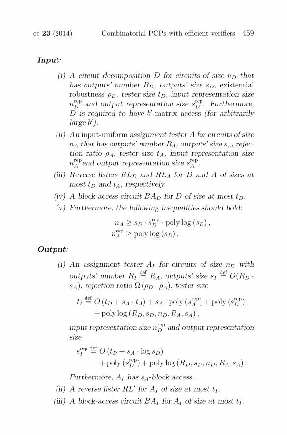
cc 23 (2014) Combinatorial PCPs with efficient verifiers 459
Input:
(i) A circuit decomposition D for circuits of size nD thathas outputs’ number RD, outputs’ size sD, existentialrobustness ρD, tester size tD, input representation sizenrep
D and output representation size srepD . Furthermore,
D is required to have b′-matrix access (for arbitrarilylarge b′).
(ii) An input-uniform assignment tester A for circuits of sizenA that has outputs’ number RA, outputs’ size sA, rejec-tion ratio ρA, tester size tA, input representation sizenrep
A and output representation size srepA .
(iii) Reverse listers RLD and RLA for D and A of sizes atmost tD and tA, respectively.
(iv) A block-access circuit BAD for D of size at most tD.
(v) Furthermore, the following inequalities should hold:
nA ≥ sD · srepD · poly log (sD) ,
nrepA ≥ poly log (sD) .
Output:
(i) An assignment tester AI for circuits of size nD with
outputs’ number RIdef= RA, outputs’ size sI
def= O(RD ·
sA), rejection ratio Ω (ρD · ρA), tester size
tIdef= O (tD + sA · tA) + sA · poly (srep
A ) + poly (srepD )
+ poly log (RD, sD, nD, RA, sA) ,
input representation size nrepD and output representation
size
srepI
def= O (tD + sA · log sD)
+ poly (srepD ) + poly log (RD, sD, nD, RA, sA) .
Furthermore, AI has sA-block access.
(ii) A reverse lister RL′ for AI of size at most tI .
(iii) A block-access circuit BAI for AI of size at most tI .
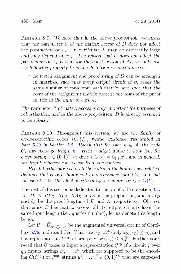
460 Meir cc 23 (2014)
Remark 8.9. We note that in the above proposition, we stressthat the parameter b′ of the matrix access of D does not affectthe parameters of AI . In particular, b′ may be arbitrarily largeand may depend on nD. The reason that b′ does not affect theparameters of AI is that for the construction of AI , we only usethe following property from the definition of matrix access:
◦ he tested assignment and proof string of D can be arrangedin matrices, such that every output circuit of ψi reads thesame number of rows from each matrix, and such that therows of the assignment matrix precede the rows of the proofmatrix in the input of each ψi.
The parameter b′ of matrix access is only important for purposes ofrobustization, and in the above proposition, D is already assumedto be robust.
Remark 8.10. Throughout this section, we use the family oferror-correcting codes {Ck}∞
k=1 whose existence was stated inFact 5.13 in Section 5.5. Recall that for each k ∈ N, the codeCk has message length k. With a slight abuse of notation, forevery string x ∈ {0, 1}∗ we denote C(x) = C|x|(x), and in general,we drop k whenever k is clear from the context.
Recall furthermore that all the codes in the family have relativedistance that is lower bounded by a universal constant δC , and thatfor each k ∈ N, the block length of Ck is denoted by lk = O(k).
The rest of this section is dedicated to the proof of Proposition 8.8.Let D, A, RLD, RLA, BAD be as in the proposition, and let �Dand �A be the proof lengths of D and A, respectively. Observethat since D has matrix access, all its output circuits have thesame input length (i.e., queries number), let us denote this lengthby qD.
Let U = UsD,srepD ,qD
be the augmented universal circuit of Corol-
lary 5.26, and recall that U has size sD ·srepD ·poly log (sD) ≤ nA and
has representation U rep of size poly log (sD) ≤ nrepA . Furthermore,
recall that U takes as input a representation ζrep of a circuit ζ overqD inputs, strings c1, . . . , cα, which are supposed to be the encod-ing C(ζrep) of ζrep, strings y1, . . . , yβ ∈ {0, 1}qD that are supposed
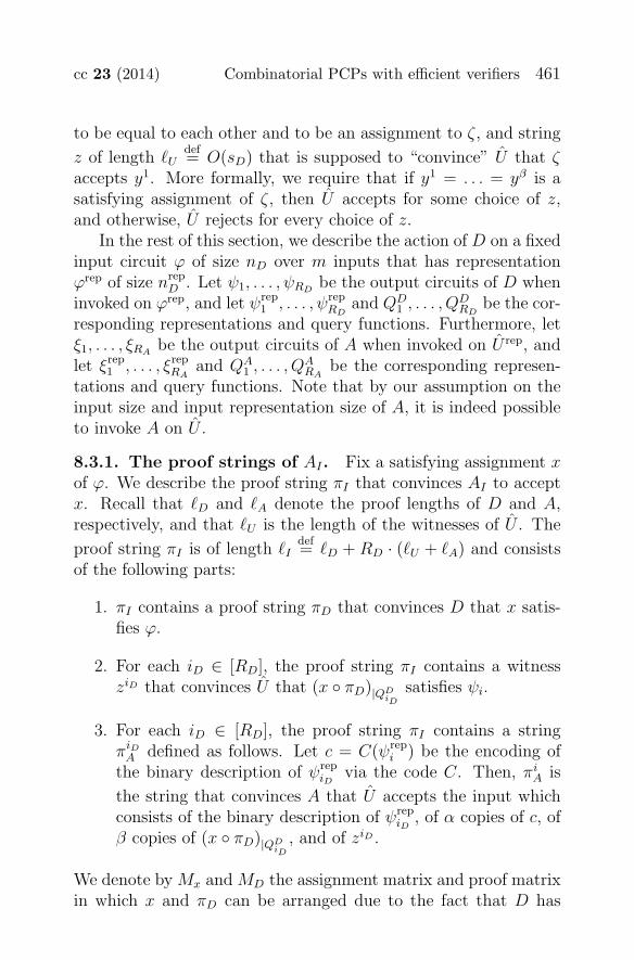
cc 23 (2014) Combinatorial PCPs with efficient verifiers 461
to be equal to each other and to be an assignment to ζ, and string
z of length �Udef= O(sD) that is supposed to “convince” U that ζ
accepts y1. More formally, we require that if y1 = . . . = yβ is asatisfying assignment of ζ, then U accepts for some choice of z,and otherwise, U rejects for every choice of z.
In the rest of this section, we describe the action of D on a fixedinput circuit ϕ of size nD over m inputs that has representationϕrep of size nrep
D . Let ψ1, . . . , ψRDbe the output circuits of D when
invoked on ϕrep, and let ψrep1 , . . . , ψrep
RDand QD
1 , . . . , QDRD
be the cor-responding representations and query functions. Furthermore, letξ1, . . . , ξRA
be the output circuits of A when invoked on U rep, andlet ξrep
1 , . . . , ξrepRA
and QA1 , . . . , Q
ARA
be the corresponding represen-tations and query functions. Note that by our assumption on theinput size and input representation size of A, it is indeed possibleto invoke A on U .
8.3.1. The proof strings of AI. Fix a satisfying assignment xof ϕ. We describe the proof string πI that convinces AI to acceptx. Recall that �D and �A denote the proof lengths of D and A,respectively, and that �U is the length of the witnesses of U . The
proof string πI is of length �Idef= �D + RD · (�U + �A) and consists
of the following parts:
1. πI contains a proof string πD that convinces D that x satis-fies ϕ.
2. For each iD ∈ [RD], the proof string πI contains a witnessziD that convinces U that (x ◦ πD)|QD
iD
satisfies ψi.
3. For each iD ∈ [RD], the proof string πI contains a stringπiD
A defined as follows. Let c = C(ψrepi ) be the encoding of
the binary description of ψrepiD
via the code C. Then, πiA is
the string that convinces A that U accepts the input whichconsists of the binary description of ψrep
iD, of α copies of c, of
β copies of (x ◦ πD)|QDiD
, and of ziD .
We denote by Mx and MD the assignment matrix and proof matrixin which x and πD can be arranged due to the fact that D has
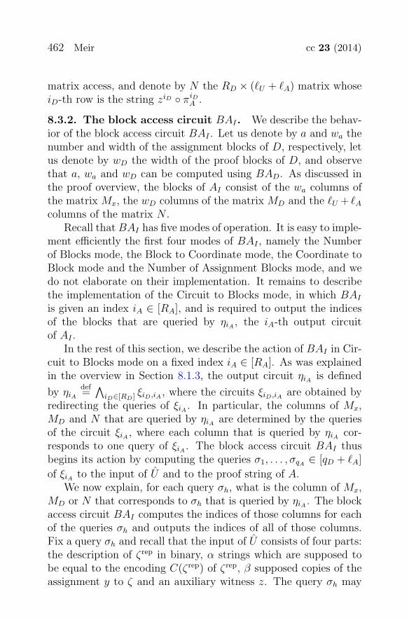
462 Meir cc 23 (2014)
matrix access, and denote by N the RD × (�U + �A) matrix whoseiD-th row is the string ziD ◦ πiD
A .
8.3.2. The block access circuit BAI. We describe the behav-ior of the block access circuit BAI . Let us denote by a and wa thenumber and width of the assignment blocks of D, respectively, letus denote by wD the width of the proof blocks of D, and observethat a, wa and wD can be computed using BAD. As discussed inthe proof overview, the blocks of AI consist of the wa columns ofthe matrix Mx, the wD columns of the matrix MD and the �U + �Acolumns of the matrix N .
Recall that BAI has five modes of operation. It is easy to imple-ment efficiently the first four modes of BAI , namely the Numberof Blocks mode, the Block to Coordinate mode, the Coordinate toBlock mode and the Number of Assignment Blocks mode, and wedo not elaborate on their implementation. It remains to describethe implementation of the Circuit to Blocks mode, in which BAI
is given an index iA ∈ [RA], and is required to output the indicesof the blocks that are queried by ηiA , the iA-th output circuitof AI .
In the rest of this section, we describe the action of BAI in Cir-cuit to Blocks mode on a fixed index iA ∈ [RA]. As was explainedin the overview in Section 8.1.3, the output circuit ηiA is defined
by ηiAdef=
∧iD∈[RD] ξiD,iA , where the circuits ξiD,iA are obtained by
redirecting the queries of ξiA . In particular, the columns of Mx,MD and N that are queried by ηiA are determined by the queriesof the circuit ξiA , where each column that is queried by ηiA cor-responds to one query of ξiA . The block access circuit BAI thusbegins its action by computing the queries σ1, . . . , σqA
∈ [qD + �A]
of ξiA to the input of U and to the proof string of A.We now explain, for each query σh, what is the column of Mx,
MD or N that corresponds to σh that is queried by ηiA . The blockaccess circuit BAI computes the indices of those columns for eachof the queries σh and outputs the indices of all of those columns.Fix a query σh and recall that the input of U consists of four parts:the description of ζrep in binary, α strings which are supposed tobe equal to the encoding C(ζrep) of ζrep, β supposed copies of theassignment y to ζ and an auxiliary witness z. The query σh may
cc 23 (2014) Combinatorial PCPs with efficient verifiers 463
be directed at any of those parts or to the proof string of A for itsinvocation on U . We consider each case separately:
1. σh is directed at z or at the proof string of A: In thiscase, if σh is directed at the u-th coordinate of z, then ηiA
queries the u-th column of N . Similarly, if σh is directedat the u-th coordinate of z, then ηiA queries the (�U + u)-thcolumn of N .
2. σh is directed at one of the supposed copies of y: Inthis case, the circuit ηiA queries one of the columns of Mx
or MD. As explained in the overview, when constructing thecircuit ξiD,iA , the queries of ξiA to the supposed copies of yare redirected to (x ◦ πD)|QD
iD
. Recall that since D has matrix
access, the string (x ◦ πD)|QDiD
consists of rows of Mx followed
by rows of MD, where the numbers of rows of Mx and MD donot depend on iD. Let us denote by ra and rD the numbers ofrows of Mx and MD, respectively, that are queried by everyoutput circuit ψiD (again, ra and rD are independent of iD).In addition, recall that we denote by wa and wD the widthsof Mx and MD.Let us view the assignment y as consisting of ra blocks oflength wa followed by rD blocks of length wD. It can be seenthat queries of ξiA to the first ra blocks are redirected by ξiD,iA
to the corresponding rows of Mx and that the following rD
blocks are always mapped to the rows of MD. Now, supposethat the query σh is directed at the v-th coordinate of one ofthe supposed copies of y. We consider two subcases:
(a) If v is the u-th coordinate of one of the first ra blocksof y, then the output circuit ηiA queries the u-th columnof Mx.
(b) On the other hand, if v is the u-th coordinate of oneof the last rD blocks of y, then the output circuit ηiA
queries the u-th column of MD.
3. σh is directed at the description of ζrep or at one of itssupposed encodings: In this case, the circuit ηiA does not
464 Meir cc 23 (2014)
query any column that corresponds to σh, since, as explainedin the overview, the queries of ξiA to ζrep and its supposedencodings are hardwired to the descriptions and encodingsof the corresponding representations ψrep
iD. This means that
the h-th input gate of each circuit ξiD,iA is hardwired to con-stants, and hence, ηiA does not make any query that corre-sponds to σh.
This concludes the description of the columns that ηiA queries, andthe description of BAI . Observe that AI indeed satisfies all therequirements for having sA-block access: every output circuit ηiA
queries at most sA columns since sA is an upper bound on thenumber of queries of ξiA . Furthermore, all the assignment blocksof AI are of the same width a. Finally, since D has matrix access,and by the definition of matrix access, it holds that every assign-ment block of AI (i.e., column of Mx) contains (1/3) fraction ofnondummy coordinates. It follows that AI has sA-block access, asrequired.
8.3.3. The implementation of AI. We proceed to describe theassignment tester AI itself. It suffices to describe the circuit modeof AI , since the query mode of AI is determined by the Circuit toBlocks mode of BAI (see Section 8.3.2), and can be implementedby using BAI . Thus, it suffices to describe, for every index iA,what is the iA-th output circuit ηiA of AI , how its representationηrep
iAis implemented and how the representation ηrep
iAis computed
by AI . For the rest of this section, fix an index iA ∈ [RA]. We focuson the descriptions of ηiA and of ηrep
iAand skip the description of
how AI computes ηrepiA
, which is straightforward.
The output circuit ηiA. We begin by describing the output cir-cuit ηiA . As explained in the overview, the basic idea that underliesthe definition of ηiA is the following: Recall that ξiA is the iA-th
output circuit of A when invoked on U . For every iD ∈ [RD], weobtain a circuit ξiD,iA from ξiA by fixing some of the queries of ξiAto the description of ψrep
iDand its encoding, and by redirecting the
other queries of ξiA into the matrices Mx, MD and N . Next, weobserve that all the queries of the circuits ξiD,iA are contained in
cc 23 (2014) Combinatorial PCPs with efficient verifiers 465
few columns of Mx, MD and N . Finally, we define ηiA to be thecircuit that queries the aforementioned columns of Mx, MD and Nand checks that that all the circuits ξiD,iA are satisfied.
More formally, the output circuit ηiA is defined as follows. Thecircuit ηiA consists of three parts:
1. Input gates.
2. An output gate which is an AND gate.
3. A collection of RD circuits, such that the iD-th circuit ξiD,iA
is obtained from ξiA by modifying ξiA as follows:
(a) Modifying the input gates of ξiD,iA that correspond to
queries to the ζrep part in the input of U to be con-stant gates that contain the description of the outputcircuit ψrep
iD.
(b) Modifying the input gates of ξiD,iA that correspond toqueries to the supposed encodings of ζrep in the inputof U to be constant gates that contain the encoding ofthe description of ψrep
iD.
(c) Connecting the output gate of ξiD,iA to the output gateof ηiA .
(d) Connecting each input gate of ξiD,iA to the correspond-ing input gate of ηiA : As explained above, every queryof ξiA should be redirected to some coordinate σ of thematrices Mx, MD and N , and ηiA queries the columninside which the coordinate σ is found. We thus con-nect each input gate of ξiD,iA that should be directed toa coordinate σ to the corresponding input gate of ηiA
that queries σ.More specifically, recall that the assignment to U con-sists of ζrep and its encodings, supposed copies of anassignment y to ζ, and of an auxiliary witness z.Furthermore, we view y as consisting of ra blocks oflength wa followed by rD blocks of length wD (see Sec-tion 8.3.2). Let qiA be the number of input gates o ξiA .
466 Meir cc 23 (2014)
For each j ∈ [qiA ], we consider the following cases forthe j-th input gate of ξiA :
i. Suppose that the j-th input gate of ξiA correspondsto a query to the u-th coordinate of the h-th blockof y (for one of the supposed copies of y). Supposefurthermore and the h-th block that is queried bythe output circuit ψiD is the v-th row of Mx or MD.Then, we connect the j-th input gate of ξiD,iA tothe input gate of ηiA that corresponds to the v-thcoordinate of the j-th column that is queried by ηiA
(which is the u-th column of Mx or MD).
ii. Suppose that the j-th input gate of ξiA correspondsto a query to the u-th coordinate of z or to the u-thcoordinate of the proof string of A. In this case, weconnect the j-th input gate of ξiA to the input gateof ηiA that corresponds to the iD-th coordinate ofthe j-th column that is queried ηiA (which is theu-th column of N).
This concludes the description of ηiA .
The representation ηrepiA
. Recall that ηrepiA
computes the follow-ing functionality: the representation ηrep
iAtakes as input the index
of a gate g of ηiA and an index h, and ηrepiA
is required to retrieve thefunction of g (one of AND, OR, NOT or one of the constants 0 and1), the index of the gate from which the h-th incoming wire of gcomes, and the index of the gate to which the h-th outgoing wire ofg goes. This functionality is straightforward to compute for mostof the gates and wires of ηiA , but is nontrivial in the following cases:
1. Suppose that g is one of the constant gates of a circuit ξiD,iA
that should be fixed to the description of ψrepiD
or its encodings.In this case, the representation ηrep
iAshould determine whether
this gate is the constant 0 or the constant 1. The straight-forward way to implement this functionality is to hardwireto the representation ηrep
iAthe descriptions of all the represen-
tations ψrepiD
for every iD ∈ [RD]. However, this would causethe representation ηrep
iAto be of size at least RD, which is
too large.
cc 23 (2014) Combinatorial PCPs with efficient verifiers 467
We therefore use the following alternative solution: We hard-wired into ηrep
iAthe input representation ϕrep and the decom-
position D itself. Then, whenever ηrepiA
needs the descriptionof ψrep
iDfor any iD ∈ [RD], the representation ηrep
iAinvokes D
on ϕrep in order to generate ψrepiD
.We stress that the fact that ηrep
iAcan compute the descrip-
tion of ψrepiD
using D is a key point in our construction of AI ,and is one of the central ideas of this work. What is actu-ally happening here is that we use the fact that the circuitsψrep
1 , . . . , ψrepiD
are in a way “similar” and “uniform,” in thesense that they can all be generated using D.We note that when ηrep
iAneeds the encoding of the description
of ψrepiD
, it computes the description of ψrepiD
and encodes it via
C, which can be done using a circuit of size poly(∣∣ψrep
iD
∣∣) =
poly (srepD ).
2. Suppose that g is an “input gate” of a circuit ξiD,iA , that is,g is one of the gates of ξiD,iA that are obtained redirecting aquery of ξiA to an input gate of ηiA . The representation ηrep
iA
should determine the gates of ηiA from which g has incomingwires, which are all input gates of ηiA . The key issue here isthat if g corresponds to a query of ξiA that is redirected to Mx
or MD, then in order to determine the relevant input gatesof ηiA , we should determine the queries of the circuit ψiD .This can be done by invoking the decomposition D on theinput representation ϕrep in query mode to obtain the queriesof ψiD , using again the fact that the descriptions of D andϕrep are hardwired into ηrep
iA.
3. Suppose that g is one of the input gates of ηiA . The represen-tation ηrep
iAshould determine the gates of ηiA to which g has
outgoing wires. All of those gates are “input gates” of circuitsξiD,iA , that is, gates of ξiD,iA that are obtained redirecting aquery of ξiA to an input gate of ηiA . The challenge is to deter-mine which are the relevant circuits ξiD,iA , that is, for whichindices iD the gate g has an outgoing wire to a gate of ξiD,iA .The key issue here is that if g corresponds to a query to acoordinate σ of Mx or MD, then we need to determine for
468 Meir cc 23 (2014)
which indices iD the output circuit ψiD queries the coordi-nate σ. Fortunately, this can be done easily by invoking thereverse lister RLD, and therefore, we hardwired the descrip-tion of RLD into ηrep
iAas well. Once we determined those
indices iD, the rest of the implementation is straightforward.Interestingly, we note that, except for the proof of Dinur’samplification theorem, this is the only place in our workwhere we use the fact that our assignment testers have super-fast reverse listers.8
We mention that we also hardwired the description of the circuit ξiAand its queries into the representation ηrep
iA. The representation ηrep
iA
uses this information to compute the descriptions of the internalgates of the circuits ξiD,iA . This concludes the implementationof ηrep
iAand the description of the circuit mode of AI .
8.3.4. The reverse lister of AI. We turn to describe the con-struction of the reverse lister RLI of AI . This construction is notcentral to the understanding of the proof of the tensor productlemma and can be skipped on first reading. We also note thatthe construction is straightforward except for one subtle point inwhich we use the assumption that the assignment tester A is input-uniform.
Fix a coordinate k ∈ [m+ �I ] and consider the action of RLI
on input representation ϕrep and coordinate k. For simplicity, weassume that k belongs to the matrix Mx, while the cases where kbelongs to one of the matrices MD and N can be handled similarly.
Recall that an output circuit ηiA decides which columns of Mx
and MD it should query as follows (see also Section 8.3.2): for eachquery of ξiA to one of the β supposed copies of y in the input of U ,the output circuit ηiA queries either a column of Mx or a columnof MD. The exact column of Mx or MD that is queried depends onthe place of the query within the supposed copy of y. In particular,if the query belongs to one of the first ra blocks of y (each of lengthwa), then ηiA queries a column of Mx, and if the query belongs to
8We also use this fact in order to upper bound the proof length, as inSection 5.2, but this is done only for convenience and can be avoided.
cc 23 (2014) Combinatorial PCPs with efficient verifiers 469
one of the last rD blocks of y (each of length wD), then ηiA queriesa column of MD.
Now, let u be the index of the column of Mx to which thecoordinate k belongs. It can be seen that there exist β · ra coor-dinates σ1, . . . , σβ·ra in the input of U such that an output cir-cuit ηiA queries the u-th column of Mx exactly once for eachquery of ξiA to a coordinate σi. Observe that the coordinatesσ1, . . . , σβ·ra can be computed efficiently from u, ra, wa, rD, wD
and qDdef= ra ·wa + rD ·wD. We turn to describe the action of RLI
on the coordinate k in each of its modes:
1. Counting mode: In this mode, RLI is given as input ϕrep
and k, and is required to output |RevListAI ,ϕ (k)|. By theabove discussion, it can be seen that
|RevListAI ,ϕ (k) | =
β·ra∑
h=1
∣∣RevListA,U (σh)
∣∣.
Now, since the assignment tester A is assumed to be input-uniform, it holds that
∣∣RevListA,U (σ1)
∣∣ =
∣∣RevListA,U (σ2)
∣∣
= . . . =∣∣RevListA,U (σβ·ra)
∣∣.
Thus, in order to compute∣∣RevListAI ,ϕ (k)
∣∣, the reverse lis-
ter RLI invokes RLA on U and σ1 to determine∣∣RevListA,U (σ1)
∣∣, and outputs β · ra · ∣
∣RevListA,U (σ1)∣∣.
2. Retrieval mode: In this mode, RLI is given as inputϕrep, k, and v ∈ [|RevListAI ,ϕ (k)|], and is required to out-put the v-th element (i, κ) of RevListAI ,ϕ (k). Recall that|RevListAI ,ϕ (k)| = β · ra · ∣∣RevListA,U (σ1)
∣∣, so the index v
can be viewed as a pair of indices (h, v′) where h ∈ [β · ra]and v′ ∈ [∣∣RevListA,U (σ1)
∣∣]. The reverse lister RLI begins
by invoking RLA in retrieval mode to compute the v′-th ele-ment (iA, κA) of RevListA,U (σh).Now, observe that the desired value of i is iA. Furthermore,observe that the place κ of the query to the coordinate k
470 Meir cc 23 (2014)
within the input of ηi can be computed efficiently using BAI .Hence, the reverse lister RLI computes this value of κ and
outputs (i, κ), where idef= iA.
3. Reverse retrieval mode: In this mode, RLI is given asinput ϕrep, k, and a pair (i, κ) ∈ RevListAI ,ϕrep (k), and isrequired to output the index v such that (i, κ) is the v-thelement of RevListAI ,ϕ (k). Recall that κ is a coordinate inthe input of ηi, and suppose that it belongs to the j-th columnthat is queried by ηi. Thus, the query of ξi that correspondsto this column is the j-th query of ξi that is not directed atthe representation ζrep or to its supposed encodings in theinput of U—suppose that this is the κA-th query of ξi. Now,the reverse lister RLI first invokes the assignment tester A inquery mode on κA to determine the coordinate σh at whichthe κA-th query of ξi is directed. Then, RLI invokes RLA inreverse retrieval mode to find the index v′ such that (i, σh) isthe v′-th element of RevListA,U (σh). Finally, RLI outputs
vdef= (h− 1) · ∣
∣RevListA,U (σ1)∣∣ + v′.
This concludes the description of the action of RLI on a coordi-nate k of Mx. The cases where k belongs to the matrix MD or tothe matrix N are handled similarly. We note that if k belongs tothe matrix N , instead of Mx or MD, then the implementation isactually simpler, since the coordinates σ1, . . . , σβ·ra in the input of
U are replaced with only one coordinate σ.
8.3.5. The parameters of AI. It is easy to verify that AI hasthe input size, input representation size, outputs’ number and out-puts’ size that are stated in the lemma. In addition, as noted inSection 8.3.2, the assignment tester AI indeed has sA-block access.We now argue that AI has the correct output representation size
srepI
def= O (tD + sA · log sD) + poly (srep
D )
+ poly log (RD, sD, nD, RA, sA) .
To see it, note that the actions of a representation ηrepiA
consist ofinvoking the decomposition D to compute a representation ψrep
iD
cc 23 (2014) Combinatorial PCPs with efficient verifiers 471
and its queries (which is a reason for the O(tD) term), computingthe encoding of ψrep
iD(which is the reason for the poly (srep
D ) term),invoking the reverse lister RLD and the block access circuit BAD
(which is another reason for the O(tD) term), and performing cal-culations on numbers in the sets [RD], [sD], [nD], [�D], [�A] and [sA](which is the reason for the term poly log (RD, sD, nD, �D, �A, sA)).Furthermore, the representation ηrep
iAcontains the description of ξiA
and all of its queries into the input of U , which is the reason forthe O (sA · log sD) term.
Next, we claim that AI indeed has tester size
tI = srepI +O (sA · tA) + sA · poly (srep
A )
= O (tD + sA · tA) + sA · poly (srepA ) + poly (srep
D )
+ poly log (RD, sD, nD, RA, sA) .
To see it, note that the actions of AI on index iA consist of com-puting the representation ξrep
iA(which accounts for a term of O(tA)),
computing the description of ξiA from ξrepiA
(which is the reasonfor the sA · poly (srep
A ) term), computing the queries of ξiA (whichaccounts for a O(sA · tA) term) and outputting the resulting repre-sentation ηiA (which accounts for the srep
I term).It remains to show that the rejection ratio of AI is Ω (ρD · ρA).
Let x be an assignment to ϕ that is ε-far from any satisfying assign-ment, and let πI be a proof string for AI . As before, we view πI asconsisting of a proof string πD for D, of a collection of witnesses zi
for U , and of a collection of proof strings πiA for A. By the existen-
tial robustness of D, there exists iD ∈ [RD] such that (x ◦ πD)|QD,ϕiD
is (ρD · ε)-far from satisfying ψiD . Now, let c = C(ψrepiD
) be encod-ing of the binary description of ψrep
iD, and consider the following
assignment y to U :
ydef= ψrep
iD◦ c ◦ · · · ◦ c︸ ︷︷ ︸
α
◦ (x ◦ πD)|QD,ϕiD
◦ · · · ◦ (x ◦ πD)|QD,ϕiD︸ ︷︷ ︸
β
◦ziD .
It is not hard to see that y is Ω (ρD · ε)-far from satisfying U ,and therefore, for at least Ω (ρA · ρD · ε) fraction of the circuits ξiAreject y ◦ πiD
A . It follows that at least Ω (ρA · ρD · ε) fraction of the
472 Meir cc 23 (2014)
circuits ξiD,iA reject their corresponding assignment, and this, inturn, implies that at least Ω (ρA · ρD · ε) fraction of the circuits ηiA
reject x ◦ πI , as required.
8.4. Proof of the tensor product lemma. In this section,we complete the proof of the tensor product lemma, by describingthe procedure of the tensor product lemma that constructs theassignment tester A from the decomposition D and the assignmenttester A′. We note that the description of the procedure and theanalysis of the parameters are technical and contain no new ideas.
When given as input a circuit decomposition D and an assign-ment tester A as in the lemma, as well as circuits RLD, BAD andRLA, the procedure takes the following steps:
1. The procedure applies the robustization technique of Propo-sition 8.6 to D, thus obtaining an existentially robust decom-position Drob.
2. The procedure applies the transformation of Lemma 5.12to A, thus obtaining an input-uniform assignment tester Auni.
3. The procedure applies Proposition 8.8 to Drob and Auni toconstruct the intermediate assignment tester AI .
4. The procedure applies Theorem 5.21 (the robustization the-orem) to AI , yielding a robust assignment tester AI′ .
5. The procedure composes AI′ with A using the compositiontheorem (Theorem 5.7), thus obtaining the assignment testerA′.
6. The procedure outputs A′ and the corresponding reverse lis-ter RL′, which is obtained in the process of constructing A′.
We turn to analyze the parameters of A′ by analyzing the parame-ters obtained in each of the foregoing steps:
1. By Proposition 8.6, it holds that Drob is a circuit decompo-
sition for circuits of size nD with outputs’ number RDrobdef=
cc 23 (2014) Combinatorial PCPs with efficient verifiers 473
2 · RD, outputs’ size sDrobdef= O(b · sD), existential robust-
ness ρDrobdef= Ω (1/b), tester size tDrob
def= O (tD) + b ·
poly log (RD, sD, nD), input representation size nrepD and out-
put representation size srepDrob
def= srep
D + b · poly log (sD). Fur-thermore, D has b′-matrix access for some arbitrary b′.
2. By Lemma 5.12, it holds that Auni is an assignment testerfor circuits of size nA with outputs’ number RAuni = 2 · RA,
outputs’ size sAunidef= O(sA), rejection ratio 1
4· ρA, tester size
tAuni = tA + poly log (nA, RA), input representation size nrepA
and output representation size srepAuni = srep
A + poly log(nA).
3. By Proposition 8.8, it holds that AI is an assignment tester
for circuits of size nD with outputs’ number RIdef= RAuni =
O(RA), outputs’ size sIdef= O(RDrob · sAuni) = O(RD · sA),
rejection ratio Ω (ρDrob · ρAuni) = Ω(ρA/b), tester size
tIdef= O (tDrob + sAuni · tAuni) + sAuni · poly
(srep
Auni
)
+ poly(srep
Drob
)
+ poly log (RDrob , sDrob , nDrob , RAuni , sAuni)
= O (tD + sA · tA) + sA · poly (srepA , log nA, logRA)
+ poly (srepD , b, log sD)
+b · poly log (RD, sD, nD, RA, sA, b) ,
input representation size nrepD , and output representation size
srepI
def= O (tDrob + sAuni · log sDrob) + poly
(srep
Drob
)
+ poly log (RDrob , sDrob , nD, RAuni , sAuni)
= O (tD + sA · log (sD · b)) + poly (srepD , b, log sD)
+ poly log (RD, sD, nD, RA, sA, b) .
Furthermore, AI has sAuni-block access. We also note that byour assumption on the input size and input representationsize of A, it is indeed legal to apply Proposition 8.8 to Drob
and Auni (recall that this proposition requires a lower boundon the input size and input representation size of A).
474 Meir cc 23 (2014)
4. By Theorem 5.21, it holds that AI′ is an assignment tester
for circuits of size nD with outputs’ number RI′def= 2 · RI =
O(RA), outputs’ size sI′def= O(sA · sI) = O (RD · s2
A), robust-
ness ρI′def= Ω (ρI/sAuni) = Ω (ρA/b · sA), tester size
tI′def= O (sAuni · tI) + sAuni · poly log (RI , sI , nD)
= O(sA · tD + s2
A · tA)
+ poly (sA, srepA , srep
D , b)
· poly log (RD, sD, nD, RA, sA, nA) ,
input representation size nrepD and output representation size
srepI′
def= srep
I + sAuni · poly log (sI)
= O (tD) + poly (srepD , b, log sD)
+sA · poly log (RD, sD, nD, RA, sA, b) .
5. Finally, by the composition theorem (Theorem 5.7), it holdsthat A′ is an assignment tester for circuits of size nD with
outputs’ number R′ def= 2 · RI · RA = O (R2
A), outputs’ size
s′ def= O(sA), rejection ratio ρ′ def
= 14
· ρI′ · ρA = Ω (ρ2A/b · sA),
tester size
t′ def= O (tI′ + tA) + poly log (nD, RI′ , �I′ , RA, �A)
= O(sA · tD + s2
A · tA)
+ poly (sA, srepA , srep
D , b)
· poly log (RD, sD, nD, RA, sA, nA) ,
input representation size nrepD and output representation size
srep′ def= srep
A + poly log(sA). Furthermore, RL′ is of size atmost t′. We also note that applying the composition theoremto AI′ and A is legal, since by our assumption on A, its inputsize is larger than sI′ , and its input representation size islarger than srep
I′ .
The required result follows.
Acknowledgements
A more detailed version of this paper was published as ECCCTR11-104 (Meir 2011). A preliminary version of this paper
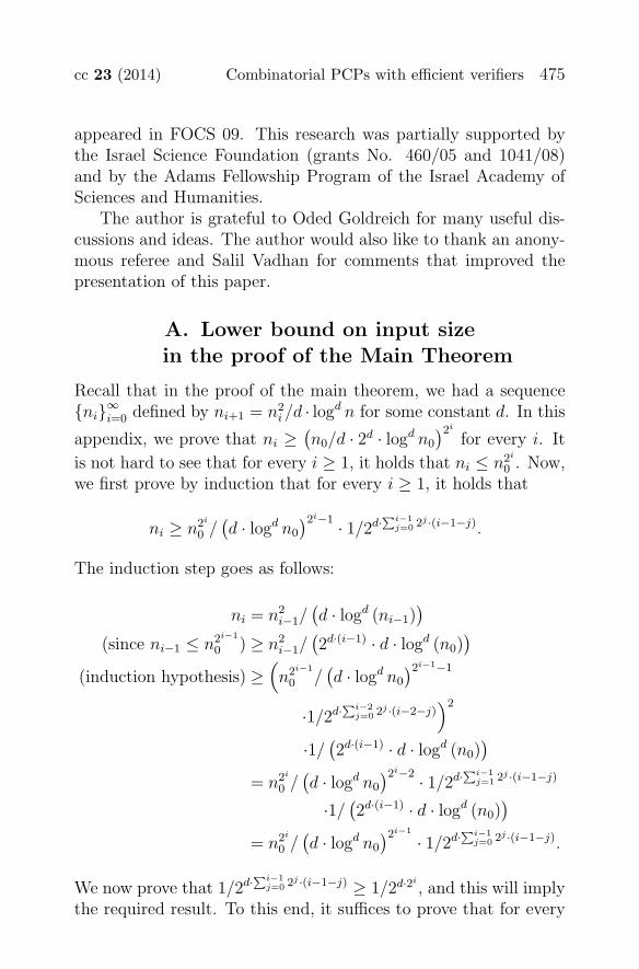
cc 23 (2014) Combinatorial PCPs with efficient verifiers 475
appeared in FOCS 09. This research was partially supported bythe Israel Science Foundation (grants No. 460/05 and 1041/08)and by the Adams Fellowship Program of the Israel Academy ofSciences and Humanities.
The author is grateful to Oded Goldreich for many useful dis-cussions and ideas. The author would also like to thank an anony-mous referee and Salil Vadhan for comments that improved thepresentation of this paper.
A. Lower bound on input sizein the proof of the Main Theorem
Recall that in the proof of the main theorem, we had a sequence{ni}∞
i=0 defined by ni+1 = n2i /d · logd n for some constant d. In this
appendix, we prove that ni ≥ (n0/d · 2d · logd n0
)2i
for every i. It
is not hard to see that for every i ≥ 1, it holds that ni ≤ n2i
0 . Now,we first prove by induction that for every i ≥ 1, it holds that
ni ≥ n2i
0 /(d · logd n0
)2i−1 · 1/2d·∑i−1j=0 2j ·(i−1−j).
The induction step goes as follows:
ni = n2i−1/
(d · logd (ni−1)
)
(since ni−1 ≤ n2i−1
0 ) ≥ n2i−1/
(2d·(i−1) · d · logd (n0)
)
(induction hypothesis) ≥(n2i−1
0 /(d · logd n0
)2i−1−1
·1/2d·∑i−2j=0 2j ·(i−2−j)
)2
·1/ (2d·(i−1) · d · logd (n0)
)
= n2i
0 /(d · logd n0
)2i−2 · 1/2d·∑i−1j=1 2j ·(i−1−j)
·1/ (2d·(i−1) · d · logd (n0)
)
= n2i
0 /(d · logd n0
)2i−1 · 1/2d·∑i−1j=0 2j ·(i−1−j).
We now prove that 1/2d·∑i−1j=0 2j ·(i−1−j) ≥ 1/2d·2i
, and this will implythe required result. To this end, it suffices to prove that for every
476 Meir cc 23 (2014)
m ≥ 0, it holds that
m∑
j=0
2j · (m− j) ≤ 2m+1
We first rewrite the sum as follows:
m∑
j=0
2j · (m− j) =m∑
j=0
2m−j · j = 2m−1
m∑
j=0
j · 2−(j−1)
So it remains to show that∑m
j=0 j · 2−(j−1) ≤ 4. Since this should
hold for everym, we actually need to show that∑∞
j=0 j ·2−(j−1) ≤ 4.The latter inequality is folklore and is proved as follows. Considerthe function
f(x) =∞∑
j=0
xj,
and its derivative
f ′(x) =∞∑
j=0
j · xj−1.
Observe that the series that we wish to upper bound is exactlyf ′(1
2). Next, observe that for x ∈ (0, 1), it holds that
f(x) =1
1 − x,
and therefore, the derivative of f in (0, 1) can also be written as
f ′(x) =1
(1 − x)2 .
Thus, the series we wish to bound converges to f ′(12) = 1
(1− 12)
2 = 4,
as required.
cc 23 (2014) Combinatorial PCPs with efficient verifiers 477
References
Sanjeev Arora, Carsten Lund, Rajeev Motwani, Madhu
Sudan & Mario Szegedy (1998). Proof verification and Intractabilityof Approximation Problems. Journal of ACM 45(3), 501–555. Prelim-inary version in FOCS 1992.
Sanjeev Arora & Shmuel Safra (1998). Probabilistic CheckableProofs: A New Characterization of NP. Journal of ACM volume 45(1),70–122. Preliminary version in FOCS 1992.
Laszlo Babai, Lance Fortnow, Leonid A. Levin & Mario
Szegedy (1991a). Checking Computations in Polylogarithmic Time.In STOC, 21–31.
Laszlo Babai, Lance Fortnow & Carsten Lund (1991b). Non-Deterministic Exponential Time has Two-Prover Interactive Protocols.Computational Complexity 1, 3–40.
Boaz Barak & Oded Goldreich (2002). Universal Arguments andtheir Applications. In IEEE Conference on Computational Complexity,194–203.
Eli Ben-Sasson, Oded Goldreich, Prahladh Harsha, Madhu
Sudan & Salil Vadhan (2006). Robust PCPs of Proximity, ShorterPCPs and Applications to Coding. SIAM Journal of Computing 36(4),120–134.
Eli Ben-Sasson, Oded Goldreich, Prahladh Harsha, Madhu
Sudan & Salil P. Vadhan (2005). Short PCPs Verifiable in Poly-logarithmic Time. In IEEE Conference on Computational Complexity,120–134.
Eli Ben-Sasson & Madhu Sudan (2008). Short PCPs with PolylogQuery Complexity. SIAM J. Comput. 38(2), 551–607. Preliminaryversion in STOC 2005.
Peter J. Cameron (1998). Combinatorics: Topics, Techniques, Algo-rithms. Cambridge University Press, Cambridge CB2 2RU, MA, USA.
Irit Dinur (2007). The PCP theorem by Gap Amplification. Journalof ACM 54(3), 241–250. Preliminary version in STOC 2006.
478 Meir cc 23 (2014)
Irit Dinur & Or Meir (2010). Derandomized Parallel Repetition ofStructured PCPs. In IEEE Conference on Computational Complexity,16–27. Full version can be obtained as ECCC TR10-107.
Irit Dinur & Omer Reingold (2006). Assignment testers: Towardscombinatorial proof of the PCP theorem. SIAM Journal of Computing36(4), 155–164.
Yuri Gurevich & Saharon Shelah (1989). Nearly Linear Time. InLogic at Botik, 108–118.
F. Thomson Leighton (1992). Introduction to parallel algorithms andarchitectures: array, trees, hypercubes. Morgan Kaufmann PublishersInc., San Francisco, CA, USA.
Florence Jessie MacWilliams & Neil James Alexander
Sloane (1988). The theory of error correcting codes. Elsevier/North-Holland, Amsterdam.
Or Meir (2011). Combinatorial PCPs with efficient verifiers. ElectronicColloquium on Computational Complexity (ECCC) 18, 104.
Or Meir (2012). Combinatorial PCPs with Short Proofs. In IEEEConference on Computational Complexity, 345–355.
Alexander Polishchuk & Daniel A. Spielman (1994). Nearly-linear size holographic proofs. In STOC, 194–203.
Daniel A. Spielman (1996). Linear-time encodable and decodableerror-correcting codes. IEEE Transactions on Information Theory42(6), 1723–1731.
Mario Szegedy (1999). Many-Valued Logics and Holographic Proofs.In ICALP, 676–686.
Manuscript received 3 August 2011
Or Meir
School of Mathematics,Institute for Advanced Study,Princeton, NJ 08540, [email protected]