combinatorial algebra for second-quantized quantum

Open Research OnlineThe Open University’s repository of research publicationsand other research outputs

Combinatorial algebra for second-quantized QuantumTheoryJournal ItemHow to cite:

Blasiak, Pawel; Duchamp, Gerard H.E.; Solomon, Allan I.; Horzela, Andrzej and Penson, Karol A. (2010).Combinatorial algebra for second-quantized Quantum Theory. Advances in Theoretical and Mathematical Physics,14(4) pp. 1209–1243.

For guidance on citations see FAQs.

c© 2011 International Press

Version: Accepted Manuscript

Link(s) to article on publisher’s website:http://dx.doi.org/doi:10.4310/atmp.2010.v14.n4.a5http://www.intlpress.com/ATMP/ATMP-issue_14_4.php

Copyright and Moral Rights for the articles on this site are retained by the individual authors and/or other copyrightowners. For more information on Open Research Online’s data policy on reuse of materials please consult the policiespage.

oro.open.ac.uk

http://oro.open.ac.uk/help/helpfaq.html

http://dx.doi.org/doi:10.4310/atmp.2010.v14.n4.a5

http://www.intlpress.com/ATMP/ATMP-issue_14_4.php

http://oro.open.ac.uk/policies.html

c© 2011 International PressAdv. Theor. Math. Phys. 14 (2010) 1209–1243

Combinatorial algebra for

second-quantized Quantum Theory

Pawel Blasiak1, Gerard H.E. Duchamp2, Allan I. Solomon3,4,Andrzej Horzela1 and Karol A. Penson3

1H. Niewodniczanski Institute of Nuclear Physics, Polish Academy ofSciences, ul. Eliasza-Radzikowskiego 152, PL 31342 Krakow, Poland

[email protected], [email protected] Galilee – Universite Paris-Nord , LIPN, CNRS UMR 7030,

99 Av. J.-B. Clement, F-93430 Villetaneuse, [email protected]

3Universite Pierre et Marie Curie, LPTMC, CNRS UMR 7600,4 pl. Jussieu, F 75252 Paris Cedex 05, France

[email protected], [email protected] and Astronomy Department, The Open University,

Milton Keynes MK7 6AA, UK

Abstract

We describe an algebra G of diagrams that faithfully gives a diagram-matic representation of the structures of both the Heisenberg–Weyl alge-bra H – the associative algebra of the creation and annihilation operatorsof quantum mechanics – and U(LH), the enveloping algebra of the Heisen-berg Lie algebra LH. We show explicitly how G may be endowed withthe structure of a Hopf algebra, which is also mirrored in the structureof U(LH). While both H and U(LH) are images of G, the algebra G hasa richer structure and therefore embodies a finer combinatorial realiza-tion of the creation–annihilation system, of which it provides a concretemodel.

e-print archive: http://lanl.arXiv.org/abs/1001.4964

1210 P. BLASIAK ET AL.

1 Introduction

One’s comprehension of abstract mathematical concepts often goes via con-crete models. In many cases, convenient representations are obtained byusing combinatorial objects. Their advantage comes from simplicity basedon intuitive notions of enumeration, composition and decomposition, whichallow for insightful interpretations, neat pictorial arguments and construc-tions [1–3]. This makes the combinatorial perspective particularly attractivefor quantum physics, due to the latter’s active pursuit of a better under-standing of fundamental phenomena. An example of such an attitude isgiven by Feynman diagrams, which provide a graphical representation ofquantum processes; these diagrams became a tool of choice in quantumfield theory [4–6]. Recently, we have witnessed major progress in this areawhich has led to a rigorous combinatorial treatment of the renormalizationprocedure [7,8] – this breakthrough came with the recognition of Hopf alge-bra structure in the perturbative expansions [9–12]. There are many otherexamples in which combinatorial concepts play a crucial role, ranging fromattempts to understand peculiar features of quantum formalism to a novelapproach to calculus, e.g., see [13–18] for just a few recent developmentsin theses directions. In the present paper, we consider some common alge-braic structures of Quantum Theory and will show that the combinatorialapproach has much to offer in this domain as well.

The current formalism and structure of Quantum Theory is based onthe theory of operators acting on a Hilbert space. According to a fewbasic postulates, the physical concepts of a system, i.e., the observablesand transformations, find their representation as operators which accountfor experimental results. An important role in this abstract description isplayed by the notions of addition, multiplication and tensor product whichare responsible for peculiarly quantum properties such as interference, non-compatibility of measurements as well as entanglement in composite systems[19–21]. From the algebraic point of view, one appropriate structure captur-ing these features is a bi-algebra or, more specifically, a Hopf algebra. Thesestructures comprise a vector space with two operations, multiplication andco-multiplication, describing how operators compose and decompose. In thefollowing, we shall be concerned with a combinatorial model that providesan intuitive picture of this type of abstract structure.

However, the bare formalism is, by itself, not enough to provide a descrip-tion of real quantum phenomena. One must also associate operators withphysical quantities. This will, in turn, involve the association of somealgebraic structure with physical concepts related to the system. In prac-tice, the most common correspondence rules are based on an associative

COMBINATORIAL ALGEBRA FOR QUANTUM THEORY 1211

algebra, the Heisenberg–Weyl algebra H. This mainly arises by analogy withclassical mechanics whose Poissonian structure is reflected in the quantum-mechanical commutator of position and momentum observables [x, p] = i�[22]. In the first instance, this commutator gives rise to a Lie algebraLH [23, 24], which naturally extends to a Hopf algebra structures in theenveloping algebra U(LH) [25, 26]. An important equivalent commutatoris that of the creation–annihilation operators [a, a†] = 1, employed in theoccupation number representation in quantum mechanics and the secondquantization formalism of quantum field theory. Accordingly, we take theHeisenberg–Weyl algebra H as our starting point.

In this paper, we develop a combinatorial approach to the Heisenberg–Weyl algebra and present a comprehensive model of this algebra in termsof diagrams. In some respects this approach draws on Feynman’s idea ofrepresenting physical processes as diagrams used as a bookkeeping tool inthe perturbation expansions of quantum field theory. We discuss natu-ral notions of diagram composition and decomposition, which provide astraightforward interpretation of the abstract operations of multiplicationand co-multiplication. The resulting combinatorial algebra G may be seenas a lifting of the Heisenberg–Weyl algebra H to a richer structure of dia-grams, capturing all the properties of the latter. Moreover, it will be shownto have a natural bi-algebra and Hopf algebra structure providing a con-crete model for the enveloping algebra U(LH) as well. Schematically, theserelationships can be pictured as follows:

Gϕ

��

��

��

ϕ

��

��

��

CombinatorialAlgebra

U(LH) π �� H Algebra

LH� �

κ

�� ι

��

Lie Algebra

where all the arrows are algebra morphisms and ϕ is a Hopf algebra mor-phism. While the lower part of the diagram is standard, the upper partand the construction of the combinatorial algebra G illustrate a genuinecombinatorial underpinning of these abstract algebraic structures.

The paper is organized as follows. In Section 2, we start by brieflyrecalling the algebraic structure of the Heisenberg–Weyl algebra H andthe enveloping algebra U(LH). In Section 3, we define the Heisenberg–Weyl diagrams and introduce the notion of composition, which leads to the


combinatorial algebra G. Section 4 deals with the concept of decomposition,endowing the diagrams with a Hopf algebra structure. The relation betweenthe combinatorial structures in G and the algebraic structures in H andU(LH) are explained as they appear in the construction. For ease of readingmost proofs have been moved to the appendices.

2 Heisenberg–Weyl algebra

The objective of this paper is to develop a combinatorial model of theHeisenberg–Weyl algebra. In order to fully appreciate the versatility of ourconstruction, we start by briefly recalling some common algebraic structuresand clarifying their relation to the Heisenberg–Weyl algebra.

2.1 Algebraic setting

An associative algebra with unit is one of the most basic structures used inthe theoretical description of physical phenomena. It consists of a vectorspace A over a field K, which is equipped with a bilinear multiplicationlaw A×A � (x, y) −→ x y ∈ A which is associative and possesses a unitelement I.1 Important notions in this framework are a basis of an algebra,by which is meant a basis for its underlying vector space structure, and theassociated structure constants. For each basis {xi} the latter are defined asthe coefficients γk

ij ∈ K in the expansion of the product xi xj =∑

k γkij xk.

We note that the structure constants uniquely determine the multiplicationlaw in the algebra.2 For example, when the underlying vector space isfinite dimensional of dimension N , that is each vector-space element has aunique expansion in terms of N basis elements, then there is only a finitenumber, at most N3, of nonvanishing γk

ij ’s. A canonical example of the (non-commutative) associative algebra with unit is a matrix algebra, or moregenerally an algebra of linear operators acting in a vector space.

A description of composite systems is obtained through the construc-tion of a tensor product. Of particular importance for physical applicationsis how the transformations distribute among the components. A canonicalexample is the algebra of angular momentum and its representation on com-posite systems. In general, this issue is properly captured by the notion ofa bi-algebra which consists of an associative algebra with unit A which is

1A full list of axioms may be found in any standard text on algebra, such as [27,28].2The structure constants must of course satisfy the constraints provided by the asso-

ciative law.


additionally equipped with a co-product and a co-unit. The co-product isdefined as a co-associative linear mapping Δ : A −→ A⊗A prescribing theaction from the algebra to a tensor product, while the co-unit ε : A −→ K

gives a linear map to the underlying field K. Furthermore, the bi-algebraaxioms require Δ and ε to be algebra morphisms, i.e., to preserve multiplica-tion in the algebra, which asserts the correct transfer of the algebraic struc-ture of A into the tensor product A⊗A. Additionally, a proper descriptionof the action of an algebra on a dual space requires the existence of an anti-morphism S : A −→ A called the antipode, thus introducing a Hopf algebrastructure in A. For a complete set of bi-algebra and Hopf algebra axiomssee [26,29,30].

In this context, it is instructive to discuss the difference between Lie alge-bras and associative algebras which is often misunderstood. A Lie algebra isa vector space L over a field K with a bilinear law L × L � (x, y) −→ [x, y] ∈L, called the Lie bracket, which is antisymmetric [x, y] = −[y, x] and satis-fies the Jacobi identity: [x, [y, z]] + [y, [z, x]] + [z, [x, y]] = 0. Lie algebras arenot associative in general3 and lack an identity element. A standard rem-edy for these deficiencies consists of passing to the enveloping algebra U(L),which has the more familiar structure of an associative algebra with unitand, at the same time, captures all the relevant properties of L. An impor-tant step in its realization is the Poincare–Birkhoff–Witt theorem whichprovides an explicit description of U(L) in terms of ordered monomials inthe basis elements of L, see [25]. As such, the enveloping algebras can beseen as giving faithful models of Lie algebras in terms of a structure withan associative law.

Below, we illustrate these abstract algebraic constructions within the con-text of the Heisenberg–Weyl algebra. These abstract algebraic concepts gainby use of a concrete example.

2.2 Heisenberg–Weyl algebra revisited

In this paper, we consider the Heisenberg–Weyl algebra, denoted byH, whichis an associative algebra with unit, generated by two elements a and a†subject to the relation

a a† = a†a + I. (2.1)

3However, all the Heisenberg Lie algebras h2n+1 are also (trivially) associative in thesense that for all x, y, z ∈ h2n+1, x � (y � z) = (x � y) � z (= 0), where � is the composition(bracket) in the Lie algebra.


This means that the algebra consists of elements A ∈ H which are linearcombinations of finite products of the generators, i.e.,

A =∑

rk,...,r1sk,...,s1

Ark,...,r1sk,...,s1

a† rk ask · · · a† r2 as2 a† r1 as1 , (2.2)

where the sum ranges over a finite set of multi-indices rk, . . . , r1 ∈ N andsk, . . . , s1 ∈ N (with the convention a0 = a† 0 = I). Throughout the paperwe stick to the notation used in the occupation number representation inwhich a and a† are interpreted as annihilation and creation operators. Wenote, however, that one should not attach too much weight to this choice aswe consider algebraic properties only, so particular realizations are irrelevantand the crux of the study is the sole relation of equation (2.1). For example,one could equally well use X as multiplication by z, and derivative operatorD = ∂z acting in the space of complex polynomials, or analytic functions,which also satisfy the relation [D, X] = I.

Observe that the representation given by equation (2.2) is ambiguous in sofar as the rewrite rule of equation (2.1) allows different representations of thesame element of the algebra, e.g., aa† or equally a†a + I. The remedy for thissituation lies in fixing a preferred order of the generators. Conventionally,this is done by choosing the normally ordered form in which all annihilatorsstand to the right of creators. As a result, each element of the algebra Hcan be uniquely written in normally ordered form as

A =∑

k,l

αkl a† k al. (2.3)

In this way, we find that the normally ordered monomials constitute a nat-ural basis for the Heisenberg–Weyl algebra, i.e.,

Basis of H : {a† kal}k,l∈N,

indexed by pairs of integers k, l = 0, 1, 2, . . ., and equation (2.3) is the expan-sion of the element A in this basis. One should note that the normallyordered representation of the elements of the algebra suggests itself not onlyas the simplest one but is also of practical use and importance in appli-cations in quantum optics [31–33] and quantum field theory [5, 34]. In thesequel, we choose to work in this particular basis. For the complete algebraicdescription of H we still need the structure constants of the algebra. Theycan be readily read off from the formula for the expansion of the product of


basis elements

a† paq a† kal =min{q,k}∑

i=0

(q

i

)(k

i

)

i! a† p+k−iaq+l−i. (2.4)

We note that working in a fixed basis is in general a nontrivial task. In ourcase, the problem reduces to rearranging a and a† to normally ordered formwhich may often be achieved by combinatorial methods [35,36].

2.3 Enveloping algebra U(LH)

We recall that the Heisenberg Lie algebra, denoted by LH,4 is a three-dimensional vector space with basis {a†, a, e} and Lie bracket defined by[a, a†] = e, [a†, e] = [a, e] = 0. Passing to the enveloping algebra involvesimposing the linear order a† � a � e and constructing the enveloping algebraU(LH) with basis given by the family

Basis of U(LH) : {a† kal em}k,l,m∈N,

which is indexed by triples of integers k, l, m = 0, 1, 2, .... Hence, elementsB ∈ U(LH) are of the form

B =∑

k,l,m

βklm a† kal em. (2.5)

According to the Poincare–Birkhoff–Witt theorem, the associative multi-plication law in the enveloping algebra U(LH) is defined by concatenation,subject to the rewrite rules

a a† = a†a + e,

e a† = a†e,e a = a e.

(2.6)

One checks that the formula for multiplication of basis elements in U(LH)is a slight generalization of equation (2.4) and is

a† paq er a† kal em =min{q,k}∑

i=0

(q

i

)(k

i

)

i! a† p+k−i aq+l−i er+m+i. (2.7)

4This Lie algebra, the Heisenberg Lie algebra, which is written here as LH, is oftencalled h3 in the literature, with h2n+1 being the extension to n creation operators.


Note that the algebra U(LH) differs from H by the additional centralelement e which should not be confused with the unity I of the envelopingalgebra.5 This distinction plays an important role in some applications asexplained below. In situations when this difference is insubstantial one mayset e→ I recovering the Heisenberg–Weyl algebra H, i.e., we have the sur-jective morphism π : U(LH) −→ H given by

π(a† iaj ek) = a† iaj . (2.8)

This completes the algebraic picture which can be subsumed in the followingdiagram:

U(LH) π �� H

LH� �

κ

�� ι

��

We emphasize that the inclusions ι : LH −→ U(LH) and κ = π ◦ ι : LH −→H are Lie algebra morphisms, while the surjection π : U(LH) −→ H is amorphism of associative algebras with unit. Note that different structuresare carried over by these morphisms.

Finally, we observe that the enveloping algebra U(LH) may be equippedwith a Hopf algebra structure. This may be constructed in a standard way bydefining the co-product6 Δ : U(LH) −→ U(LH)⊗ U(LH) on the generatorsx = a†, a, e setting Δ(x) = x⊗ I + I ⊗ x, which further extends to

Δ(a† paq er) =∑

i,j,k

(p

i

)(q

j

)(r

k

)

a† iaj ek ⊗ a† p−iaq−j er−k. (2.9)

Similarly, the antipode S : U(LH) −→ U(LH) is given on generators byS(x) = −x, and hence from the anti-morphism property yields

S(a† paq er) = (−1)p+q+r er aq a† p. (2.10)

Finally, the co-unit ε : U(LH) −→ K is defined in the following way:

ε(a† paq er

)=

{1, if p, q, r = 0,

0, otherwise.(2.11)

A word of warning here: the Heisenberg–Weyl algebraH can not be endowedwith a bi-algebra structure contrary to what is sometimes tacitly assumed.

5As usual, we write a0 = a†0= e0 = I.

6Note that this definition gives a co-commutative Hopf algebra. One may also definea nonco-commutative co-product [37].


This is because properties of the co-unit contradict the relation of equa-tion (2.1), i.e., it follows that ε(I) = ε(a a† − a†a) = ε(a) ε(a†)− ε(a†) ε(a) =0 while one should have ε(I) = 1. This brings out the importance of theadditional central element e = I which saves the day for U(LH).

3 Algebra of diagrams and composition

In this section, we define the combinatorial class of Heisenberg–Weyl dia-grams which is the central object of our study. We equip this class withan intuitive notion of composition, permitting the construction of an alge-bra structure and thus providing a combinatorial model of the algebras Hand U(LH). See [38] for a comprehensive combinatorial background of thisconstruction.

3.1 Combinatorial concepts

We start by recalling a few basic notions from graph theory [39] needed fora precise definition of the Heisenberg–Weyl diagrams, and then provide anintuitive graphical representation of this structure.

Briefly, from a set-theoretical point of view, a directed graph is a collectionof edges E and vertices V with the structure determined by two mappingsh, t : E −→ V prescribing how the head and tail of an edge are attachedto vertices. Here we address a slightly more general setting consisting ofpartially defined graphs whose edges may have one of the ends free (but notboth), i.e., we consider finite graphs with partially defined mappings h andt such that dom(h) ∪ dom(t) = E, where dom stands for domain. Addition-ally, we exclude the possibility of isolated vertices, i.e., each vertex in a graphis attached to some edge codom(h) ∪ codom(t) = V , where codom denotescodomain. We call a cycle in a graph any sequence of edges e1, e2, . . . , en

such that h(ek) = t(ek+1) for k < n and h(en) = t(e1). A convenient conceptin graph theory concerns the notion of equivalence. Two graphs given byh1, t1 : E1 −→ V1 and h2, t2 : E2 −→ V2 are said to be equivalent if one canbe isomorphically transformed into the other, i.e., both have the same num-ber of vertices and edges and there exist two isomorphisms αE : E1 −→ E2

and αV : V1 −→ V2 faithfully transferring the structure of the graphs in thefollowing sense:

E1h ��t

��

αE

��

V1

αV

��E2

h ��t

�� V2


The advantage of equivalence classes so defined is that we can liberate our-selves from specific set-theoretical realizations and think of a graph onlyin terms of relations between vertices and edges which can be convenientlydescribed in a graphical way – this is the attitude we adopt in the sequel.

In this context, we propose the following formal definition:

Definition 3.1 (Heisenberg–Weyl diagrams). A Heisenberg–Weyl diagramΓ is a class of partially defined directed graphs without cycles. It consistsof three sorts of lines: the inner ones Γ

0 having both head and tail attachedto vertices, the incoming lines Γ

− with free tails, and the outgoing lines Γ+

with free heads.

A typical modus operandi when working with classes is to invoke rep-resentatives. Following this practice, by default we make all statementsconcerning Heisenberg–Weyl diagrams with reference to its representatives,assuming that they are class invariants, which assumption can be routinelychecked in each case.

The formal Definition 3.1 gives an intuitive picture in graphical form –see the illustration figure 1. A diagram can be represented as a set ofvertices • connected by lines each carrying an arrow indicating the directionfrom the tail to the head. Lines having one of the ends not attached to avertex will be marked with � or �� at the free head or tail, respectively. Wewill conventionally draw all incoming lines at the bottom and the outgoinglines at the top with all arrows heading upwards; this is always possiblesince the diagrams do not have cycles. This pictures the Heisenberg–Weyldiagram as a sort of process or transformation with vertices playing the roleof intermediate steps.

Figure 1: An example of a Heisenberg–Weyl diagram with three distin-guished characteristic sorts of lines: the inner ones |Γ 0| = 4, the incominglines |Γ−| = 4 and outgoing lines |Γ+| = 3.


An important characteristic of a diagram Γ is the total number of its linesdenoted by |Γ |. In the next sections, we further refine counting of the linesto the inner, the incoming and the outgoing lines, denoting the result by|Γ 0|, |Γ−| and |Γ+|, respectively. Clearly, one has |Γ | = |Γ 0|+ |Γ−|+ |Γ+|.

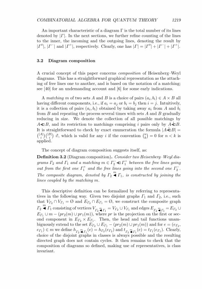
3.2 Diagram composition

A crucial concept of this paper concerns composition of Heisenberg–Weyldiagrams. This has a straightforward graphical representation as the attach-ing of free lines one to another, and is based on the notation of a matching;see [40] for an undemanding account and [6] for some early indications.

A matching m of two sets A and B is a choice of pairs (ai, bi) ∈ A×B allhaving different components, i.e., if ai = aj or bi = bj then i = j. Intuitively,it is a collection of pairs (ai, bi) obtained by taking away ai from A and bi

from B and repeating the process several times with sets A and B graduallyreducing in size. We denote the collection of all possible matchings byA��B, and its restriction to matchings comprising i pairs only by A��i B.It is straightforward to check by exact enumeration the formula |A��i B| =(|A|

i

)(|B|i

)i!, which is valid for any i if the convention

(nk

)= 0 for n < k is

applied.

The concept of diagram composition suggests itself, as:

Definition 3.2 (Diagram composition). Consider two Heisenberg–Weyl dia-grams Γ2 and Γ1 and a matching m ∈ Γ

−2 ��Γ

+

1 between the free lines goingout from the first one Γ

+

1 and the free lines going into the second one Γ−2 .

The composite diagram, denoted by Γ2m� Γ1, is constructed by joining the

lines coupled by the matching m.

This descriptive definition can be formalized by referring to representa-tives in the following way. Given two disjoint graphs Γ1 and Γ2, i.e., suchthat VΓ2 ∩ VΓ1 = Ø and EΓ2 ∩ EΓ1 = Ø, we construct the composite graphΓ2

m� Γ1 consisting of vertices V

Γ2 �m Γ1= VΓ2 ∪ VΓ1 and edges E

Γ2 �m Γ1= EΓ2 ∪

EΓ1 ∪m− (pr2(m) ∪ pr1(m)), where pr is the projection on the first or sec-ond component in EΓ2 × EΓ1 . Then, the head and tail functions unam-biguously extend to the set EΓ2 ∪ EΓ1 − (pr2(m) ∪ pr1(m)) and for e = (eΓ2 ,eΓ1) ∈ m we define h

Γ2 �m Γ1(e) = hΓ2(eΓ2) and t

Γ2 �m Γ1(e) = tΓ1(eΓ1). Clearly,

choice of the disjoint graphs in classes is always possible and the resultingdirected graph does not contain cycles. It then remains to check that thecomposition of diagrams so defined, making use of representatives, is classinvariant.


Figure 2: Composition of two diagrams Γ2m� Γ1 according to the matching

m ∈ Γ−2 ��Γ

+

1 consisting of three connections.

Definition 3.2 can be straightforwardly seen as if diagrams were put overone another with some of the lines going out from the lower one pluggedinto some of the lines going into the upper one in accordance with a givenmatching m ∈ Γ

−2 ��Γ

+

1 , for illustration see figure 2. Observe that in gen-eral two graphs can be composed in many ways, i.e., as many as there arepossible matchings (elements in Γ

−2 ��Γ

+

1 ). In Section 3.3, we exploit allthese possible compositions to endow the diagrams with the structure ofan algebra. Note also that the above construction depends on the orderin which diagrams are composed and in general the reverse order yieldsdifferent results.

We conclude by two simple remarks concerning the composition of twodiagrams Γ2 and Γ1 constructed by joining exactly i lines. Firstly, we observethat possible compositions can be enumerated explicitly by the formula

|Γ−2 ��i Γ

+

1 | =(|Γ−

2 |i

)(|Γ+

1 |i

)

i!. (3.1)

Secondly, the number of incoming, outgoing and inner lines in the composeddiagram does not depend on the choice of a matching m ∈ Γ

−2 ��i Γ

+

1 and


reads, respectively,

|(Γ2m� Γ1)

+| = |Γ+

2 |+ |Γ+

1 | − i,

|(Γ2m� Γ1)

−| = |Γ−2 |+ |Γ−

1 | − i,

|(Γ2m� Γ1)

0| = |Γ 0

2 |+ |Γ 0

1 |+ i. (3.2)

3.3 Algebra of Heisenberg–Weyl diagrams

We show here that the Heisenberg–Weyl diagrams come equipped with anatural algebraic structure based on diagram composition. It will appear tobe a combinatorial refinement of the familiar algebras H and U(LH).

An algebra requires two operations, addition and multiplication, whichwe construct in the following way. We define G as a vector space over K

generated by the basis set consisting of all Heisenberg–Weyl diagrams, i.e.,

G ={∑

iαi Γi : αi ∈ K, Γi – Heisenberg–Weyl diagram

}. (3.3)

Addition and multiplication by scalars in G has the usual form∑

iαi Γi +

∑

iβi Γi =

∑

i(αi + βi) Γi, (3.4)

and

β∑

iαi Γi =

∑

iβ αi Γi. (3.5)

The nontrivial part in the definition of the algebra G concerns multiplication,which by bilinearity

∑

iαi Γi ∗

∑

jβj Γj =

∑

i,jαiβj Γi ∗ Γj , (3.6)

reduces to determining it on the basis set of the Heisenberg–Weyl diagrams.Recalling the notions of Section 3.2, we define the product of two diagramsΓ2 and Γ1 as the sum of all possible compositions, i.e.,

Γ2 ∗ Γ1 =∑

m∈Γ−2 ��Γ

+1

Γ2m� Γ1. (3.7)

Clearly, the sum is well defined as there is only a finite number of com-positions (elements in Γ

−2 ��Γ

+

1 ). Note that although all coefficients in


equation (3.7) are equal to one, some terms in the sum may appear severaltimes giving rise to nontrivial structure constants. The multiplication thusdefined is noncommutative and possesses a unit element which is the emptygraph Ø (no vertices, no lines). Moreover, the following theorem holds (forthe proof of associativity see Appendix A):

Theorem 3.1 (Algebra of diagrams). Heisenberg–Weyl diagrams form a(noncommutative) associative algebra with unit (G, +, ∗, Ø).

Our objective, now, is to clarify the relation of the algebra of Heisenberg–Weyl diagrams G to the physically relevant algebras U(LH) and H. We shallconstruct forgetful mappings which give a simple combinatorial prescriptionof how to obtain the two latter structures from G.

We define a linear mapping ϕ : G −→ U(LH) on the basis elements by

ϕ(Γ ) = a† |Γ+| a|Γ

−| e|Γ0|. (3.8)

This prescription can be intuitively understood by looking at the diagrams asif they were carrying auxiliary labels a†, a and e attached to all the outgoing,incoming and inner lines, respectively. Then the mapping of equation (3.8)just neglects the structure of the graph and only pays attention to the num-ber of lines, i.e., counting them according to the labels. Clearly, ϕ is ontoand it can be proved to be a genuine algebra morphism, i.e., it preservesaddition and multiplication in G (for the proof see Appendix B).

Similarly, we define the morphism ϕ : G −→ H as

ϕ(Γ ) = a†|Γ+| a|Γ

−|, (3.9)

which differs from ϕ by ignoring all inner lines in the diagrams. It can beexpressed as ϕ = π ◦ ϕ and hence satisfies all the properties of an algebramorphism.

We recapitulate the above discussion in the following theorem:

Theorem 3.2 (Forgetful mapping). The mappings ϕ : G −→ U(LH) andϕ : G −→ H defined in equations (3.8) and (3.9) are surjective algebra mor-phisms, and the following diagram commutes

Gϕ

��

��

�ϕ

��

��

�

U(LH) π �� H(3.10)


Therefore, the algebra of Heisenberg–Weyl diagrams G is a lifting of thealgebras U(LH) and H, and the latter two can be recovered by applyingappropriate forgetful mappings ϕ and ϕ. As such, the algebra G can be seenas a fine graining of the abstract algebras U(LH) and H. Thus, these latteralgebras gain a concrete combinatorial interpretation in terms of the richerstructure of diagrams.

4 Diagram decomposition and Hopf algebra

We have seen in Section 3 how the notion of composition allows for a combi-natorial definition of diagram multiplication, opening the door to the realmof algebra. Here, we consider the opposite concept of diagram decomposi-tion which induces a combinatorial co-product in the algebra, thus endowingHeisenberg–Weyl diagrams with a bi-algebra structure [38]. Furthermore,we will show that G forms a Hopf algebra as well.

4.1 Basic concepts: combinatorial decomposition

Suppose we are given a class of objects which allow for decomposition, i.e.,split into ordered pairs of pieces from the same class. Without loss of gen-erality one may think of the class of Heisenberg–Weyl diagrams and some,for the moment unspecified, procedure assigning to a given diagram Γ itspossible decompositions (Γ ′′, Γ ′). In general, there might be various waysof splitting an object according to a given rule and, moreover, some of themmay yield the same result. We denote the collection of all possibilities by〈Γ 〉 = {(Γ ′′, Γ ′)} and for brevity write

Γ � (Γ ′′, Γ ′) ∈ 〈Γ 〉. (4.1)

Note that strictly 〈Γ 〉 is a multiset, i.e., it is like a set but with arbitraryrepetitions of elements allowed. Hence, in order not to overlook any of thedecompositions, some of which may be the same, we should use a moreappropriate notation employing the notion of a disjoint union, denoted by⊎

, and write〈Γ 〉 =

⊎

decompositionsΓ�(Γ ′′,Γ ′)

{(Γ ′′, Γ ′)}. (4.2)

The concept of decomposition is quite general at this point and its furtherdevelopment obviously depends on the choice of the rule. One usually sup-plements this construction with additional constraints. Below we discusssome natural conditions one might expect from a decomposition rule.


(0) Finiteness. It is reasonable to assume that an object decomposes in afinite number of ways, i.e., for each Γ the multiset 〈Γ 〉 is finite.

(1) Triple decomposition. Decomposition into pairs naturally extends tosplitting an object into three pieces Γ � (Γ3, Γ2, Γ1). An obvious wayto carry out the multiple splitting is by applying the same proce-dure repeatedly, i.e., decomposing one of the components obtainedin the preceding step. However, following this prescription one usuallyexpects that the result does not depend on the choice of the componentit is applied to. In other words, we require that we end up with thesame collection of triple decompositions when splitting Γ � (Γ ′′, Γ1)and then splitting the left component Γ ′′ � (Γ3, Γ2), i.e.,

Γ � (Γ ′′, Γ1) � (Γ3, Γ2, Γ1), (4.3)

as in the case when starting with Γ � (Γ3, Γ′) and then splitting the

right component Γ ′ � (Γ2, Γ1), i.e.,

Γ � (Γ3, Γ′) � (Γ3, Γ2, Γ1). (4.4)

This condition can be seen as the co-associativity property for decom-position, and in explicit form boils down to the following equality:

⊎

(Γ ′′,Γ1)∈〈Γ 〉(Γ3,Γ2)∈〈Γ ′′〉

{(Γ3, Γ2, Γ1)} =⊎

(Γ3,Γ ′)∈〈Γ 〉(Γ2,Γ1)∈〈Γ ′〉

{(Γ3, Γ2, Γ1)}. (4.5)

The above procedure straightforwardly extends to splitting into mul-tiple pieces Γ � (Γn, . . . , Γ1). Clearly, the condition of equation (4.5)entails the analogous property for multiple decompositions.

(2) Void object. Often, in a class there exists a sort of a void (or empty - weuse both terms synonymously) element Ø, such that objects decomposein a trivial way. It should have the property that any object Γ = Øsplits into a pair containing either Ø or Γ in two ways only

Γ � (Ø, Γ ) and Γ � (Γ, Ø), (4.6)

and Ø � (Ø, Ø). Clearly, if Ø exists, it is unique.(3) Symmetry. For some rules the order between components in decompo-

sitions is immaterial, i.e., the rule allows for an exchange (Γ ′, Γ ′′)←→(Γ ′′, Γ ′). In this case the following symmetry condition holds:

(Γ ′, Γ ′′) ∈ 〈Γ 〉 ⇐⇒ (Γ ′′, Γ ′) ∈ 〈Γ 〉, (4.7)

and the multiplicities of (Γ ′, Γ ′′) and (Γ ′′, Γ ′) in 〈Γ 〉 are the same.


(4) Composition–decomposition compatibility. Suppose that in addition todecomposition we also have a well-defined notion of composition ofobjects in the class. We denote the multiset comprising all possiblecompositions of Γ2 with Γ1 by Γ2 � Γ1, e.g., for the Heisenberg–Weyldiagrams we have

Γ2 � Γ1 =⊎

m∈Γ−2 ��Γ

+1

Γ2m� Γ1. (4.8)

Now, given a pair of objects Γ2 and Γ1, we may think of two consistentdecomposition schemes which involve composition. We can either startby composing them together Γ2 � Γ1 and then splitting all resultingobjects into pieces, or first decompose each of them separately into〈Γ2〉 and 〈Γ1〉 and then compose elements of both sets in a componen-twise manner. One may require that the outcomes are the same nomatter which way the procedure goes. Hence, a formal description ofcompatibility comes down to the equality

⊎

Γ∈Γ2�Γ1

〈Γ 〉 =⊎

(Γ ′′2 ,Γ ′

2)∈〈Γ2〉(Γ ′′

1 ,Γ ′1)∈〈Γ1〉

(Γ ′′2 � Γ ′′

1 )× (Γ ′2 � Γ ′

1). (4.9)

We remark that this property indicates that the void object Ø of con-dition (2) is the same as the neutral element for composition.

(5) Finiteness of multiple decompositions. Recall the process of multi-ple decompositions Γ � (Γn, . . . , Γ1) constructed in condition (1) andobserve that one may extend the number of components to any n ∈ N.However, if one considers only nontrivial decompositions which do notcontain void components Ø it is often the case that the process termi-nates after a finite number of steps. In other words, for each Γ thereexists N ∈ N such that

{Γ � (Γn, . . . , Γ1) : Γn, . . . , Γ1 = Ø} = ∅ (4.10)

for n > N . In practice, objects usually carry various characteristicscounted by natural numbers, e.g., the number of elements they arebuilt from. Then, if the decomposition rule decreases such a character-istic in each of the components in a nontrivial splitting, it inevitablyexhausts and then the condition of equation (4.10) is automaticallyfulfilled.

Having discussed the above quite general conditions expected from a rea-sonable decomposition rule we are now in a position to return to the realm


of algebra. We have already seen in Section 3.3 how the notion of compo-sition induces a multiplication which endows the class of Heisenberg–Weyldiagrams with the structure of an algebra, see Theorem 3.1. Following thisroute we now employ the concept of decomposition to introduce the struc-ture of a Hopf algebra in G. A central role in the construction will be playedby the three mappings given below.

Let us consider a linear mapping Δ : G −→ G ⊗ G defined on the basiselements as a sum of possible splittings, i.e.,

Δ(Γ ) =∑

(Γ ′,Γ ′′)∈〈Γ 〉Γ ′ ⊗ Γ ′′. (4.11)

Note, that although all coefficients in equation (4.11) are equal to one, someterms in the sum may appear several times. This is because elements inthe multiset 〈Γ 〉 may repeat and the numbers counting their multiplicitiesare sometimes called section coefficients [41]. Observe that the sum is welldefined as long the number of decompositions is finite, i.e., condition (0) issatisfied.

We also make use of a linear mapping ε : G −→ K which extracts thecoefficient of the void element Ø. It is defined on the basis elements by

ε(Γ ) =

{1, if Γ = Ø,

0, otherwise.(4.12)

Finally, we need a linear mapping S : G −→ G defined by the formula

S(Γ ) =∑

Γ�(Γn,··· ,Γ1)Γn,...,Γ1 �=∅

(−1)n Γn ∗ . . . ∗ Γ1, (4.13)

for Γ = Ø and S(Ø) = Ø. Note that it is an alternating sum over productsof nontrivial multiple decompositions of an object. Clearly, if the condition(5) holds the sum is finite and S is well defined.

The mappings Δ, ε and S, built upon a reasonable decomposition proce-dure, provide G with a rich algebraic structure as summarized in the follow-ing lemma (for the proofs see Appendix C):

Lemma 4.1 (Decomposition and Hopf algebra).

(i) If the conditions (0), (1) and (2) are satisfied, the mappings Δ and εdefined in equations (4.11) and (4.12) are the co-product and co-unit in


the algebra G. The co-algebra (G, Δ, ε) thus defined is co-commutative,provided condition (3) is fulfilled.

(ii) In addition, if condition (4) holds we have a genuine bi-algebra struc-ture (G, +, ∗, Ø, Δ, ε).

(iii) Finally, under condition (5) we establish a Hopf algebra structure(G, +, ∗, Ø, Δ, ε, S) with the antipode S defined in equation (4.13).

We remark that the above discussion is applicable to a wide range ofcombinatorial classes and decomposition rules which we have thus far leftunspecified. Below, we apply these concepts to the class of Heisenberg–Weyldiagrams.

4.2 Hopf algebra of Heisenberg–Weyl diagrams

In this section, we provide an explicit decomposition rule for the Heisenberg–Weyl diagrams satisfying all the conditions discussed in Section 4.1. In thisway, we complete the whole picture by introducing a Hopf algebra structureon G.

We start by observing that for a given Heisenberg–Weyl graph Γ , eachsubset of its edges L ⊂ EΓ induces a subgraph Γ |L which is defined byrestriction of the head and tail functions to the subset L. Likewise, theremaining part of the edges R = EΓ − L gives rise to a subgraph Γ |R.Clearly, the results are again Heisenberg–Weyl graphs. Thus, by consid-ering ordered partitions of the set of edges into two subsets L + R = EΓ ,i.e., L ∪R = EΓ and L ∩R = ∅, we end up with pairs of disjoint graphs(Γ |L, Γ |R). This suggests the following definition:

Definition 4.1 (Diagram decomposition). A decomposition of aHeisenberg–Weyl diagram Γ is any splitting (ΓL, ΓR) induced by an orderedpartition of its lines L + R = EΓ . Hence, the multiset 〈Γ 〉 comprising allpossible decompositions can be indexed by the set of ordered double partitions{(L, R) : L + R = EΓ }, and we have

〈Γ 〉 =⊎

L+R=EΓ

{(Γ |L, Γ |R)}. (4.14)

The graphical picture is clear: the decomposition of a diagram Γ � (Γ |L,Γ |R) is defined by the choice of lines L ⊂ EΓ , which taken out make upthe first component of the pair while the remainder induced by R = EΓ − Lconstitutes the second one. (See the illustration in figure 3.)


Figure 3: An example of diagram decomposition Γ � (Γ |L, Γ |R). Thechoice of edges L ⊂ EΓ inducing the diagram Γ |L is depicted on the leftdiagram as dashed lines.

We observe that the enumeration of all decompositions of a diagram Γ isstraightforward since the multiset 〈Γ 〉 can be indexed by subsets of EΓ .Because |EΓ | = |Γ |, explicit counting gives |〈Γ 〉| = ∑

i

(|Γ |i

)= 2|Γ |. This

simple observation can be generalized to calculate the number of decom-positions (Γ |L, Γ |R) ∈ 〈Γ 〉 in which the first component has i outgoing, j

incoming and k inner lines, i.e., |Γ |+L| = i, |Γ |−L| = j, |Γ |0L| = k. Accordingly,the enumeration reduces to the choice of i, j and k lines out of the sets Γ

+,Γ

− and Γ0 respectively, which gives

∣∣∣∣∣∣

⎧⎨

⎩(Γ |L, Γ |R) ∈ 〈Γ 〉 :

|Γ |+L |=i

|Γ |−L |=j

|Γ |0L|=k

⎫⎬

⎭

∣∣∣∣∣∣=

(|Γ+|i

)(|Γ−|j

)(|Γ 0|k

)

. (4.15)

Of course, the second component Γ |R is always determined by the firstone Γ |L and hence the number of its outgoing, incoming and inner lines isgiven by

|Γ |+R| = |Γ+| − i,

|Γ |−R| = |Γ−| − j,

|Γ |0R| = |Γ 0| − k.

(4.16)

Having explicitly defined the notion of diagram decomposition, one maycheck that it satisfies conditions (1)–(5) of Section 4.1; for the proofs seeAppendix D. In this context, equation (4.11) defining the co-product in thealgebra G takes the form

Δ(Γ ) =∑

L+R=EΓ

Γ |L ⊗ Γ |R, (4.17)


and the antipode of equation (4.13) may be rewritten as

S(Γ ) =∑

An+...+A1=EΓAn,...,A1 �=∅

(−1)n Γ |An ∗ · · · ∗ Γ |A1 . (4.18)

for Γ = Ø and S(Ø) = Ø. Therefore, referring to Lemma 4.1, we supplementTheorem 3.1 by the following result:

Theorem 4.1 (Hopf algebra of diagrams). The algebra of Heisenberg–Weyldiagrams G has a Hopf algebra structure (G, +, ∗, Ø, Δ, ε, S) with(co-commutative) co-product, co-unit and antipode as defined in equations(4.17), (4.12) and (4.18), respectively.

The algebra of Heisenberg–Weyl diagrams G was shown to be directlyrelated to the algebra U(LH) through the forgetful mapping ϕ which pre-serves algebraic operations as explained in Theorem 3.2. Here, however,in the context of Theorem 4.1 the algebra G is additionally equipped witha co-product, co-unit and antipode. Since U(LH) is also a Hopf algebra,it is natural to ask whether this extra structure is preserved by the mor-phism ϕ of equation (3.8). It turns out that indeed it is also preserved,and one can augment Theorem 3.2 in the following way (for the proof seeAppendix B):

Theorem 4.2 (Hopf algebra morphism ϕ). The forgetful mapping ϕ : G −→U(LH) defined in equation (3.8) is a Hopf algebra morphism.

In this way, we have extended the results of Section 3 to encompass theHopf algebra structure of the enveloping algebra U(LH). This completesthe picture of the algebra of Heisenberg–Weyl diagrams G as a combinato-rial model which captures all the relevant properties of the algebras H andU(LH).

5 Conclusions

The development of concrete models in physics often provides a means ofunderstanding abstract algebraic constructs in a more natural way. Thisappears to be particularly valuable in the realm of Quantum Theory, where


the abstract formalism is far from intuitive. In this respect, the combina-torial perspective seems to provide a promising approach, and as such hasbecome a blueprint for much contemporary research. For example, recentwork in perturbative Quantum Field Theory (pQFT) has shown the valueof analyzing the algebraic structure of a diagrammatic approach, in thecase of pQFT, that of the Feynman diagrams [7]. The present work differsfrom that discussing pQFT in several respects. Standard nonrelativisticsecond-quantized Quantum Theory, in which context the present study isfirmly based, does not suffer from the singularities which plague pQFT. Asa consequence, well-understood procedures will, at least in principle, sufficeto analyze models based on nonrelativistic Quantum Theory. Nevertheless,the value both of a diagrammatic approach – even in the nonrelativistic case– as well as an analysis of the underlying algebraic structure – can only leadto a deeper understanding of the theory. In this note, we described perhapsthe most basic structure of Quantum Theory, that involving a single modesecond-quantized theory.7 In spite of this simple model, the underlyingalgebraic structure proves to be surprisingly rich.8

The standard commutation relation between a single creation and anni-hilation operator of second-quantized quantum mechanics, a a† − a†a = I,generates in a natural way the Heisenberg–Weyl associative algebra H, aswell as the Heisenberg Lie algebra LH and its enveloping algebra U(LH). Wediscussed these algebras, showing, inter alia, that U(LH) can be endowedwith a Hopf algebra structure, unlike H. However, the main content of thecurrent work was the introduction of a combinatorial algebra G of graphs,arising from a diagrammatic representation of the creation–annihilationoperator system. This algebra was shown to carry a natural Hopf struc-ture. Further, it was proved that both H and U(LH) were homomorphicimages of G, in the latter case a true Hopf algebra homomorphism.

Apart from giving a concrete and visual representation of the a and a†actions, the algebra G remarkably exhibits a finer structure than either ofthe algebras H or U(LH). This “fine graining” of the effective actions of thecreation–annihilation operators implies a richer structure for these actions,possibly leading to a deeper insight into this basic quantum mechanicalsystem. Moreover, we should point out that the diagrammatic model ofthe Heisenberg–Weyl algebra presented here is particularly suited to themethods of modern combinatorial analysis [1–3]; this aspect is extensivelydiscussed in the paper [42].

7One does not expect that the extension to several commuting modes would introduceadditional complication.

8Of course, this is not identical to the Connes–Kreimer algebra arising in pQFT.


Appendix A Associativity of multiplication in G

We prove associativity of the multiplication defined in equation (3.7). Frombilinearity, we need only check it for the basis elements, i.e.,

Γ3 ∗ (Γ2 ∗ Γ1) = (Γ3 ∗ Γ2) ∗ Γ1. (A.1)

Written explicitly, the left- and right-hand sides of this equation take theform

Γ3 ∗ (Γ2 ∗ Γ1) =∑

m′

∑

m21

Γ3m′� (Γ2

m21� Γ1), (A.2)

where m′ ∈ Γ−3 ��(Γ2

m21� Γ1)+ and m21 ∈ Γ

−2 ��Γ

+

1 , while

(Γ3 ∗ Γ2) ∗ Γ1 =∑

m32

∑

m′′(Γ3

m32� Γ2)m′′� Γ1, (A.3)

where m32 ∈ Γ−3 ��Γ

+

2 and m′′ ∈ (Γ3m32� Γ2)

−��Γ+

1 .

Consider the double sums in the above equations, indexed by (m′, m21),and (m32, m

′′), respectively, and observe that there exists a one-to-one cor-respondence between their elements. We construct it by a fine graining ofthe matchings, see figure A.1, and define the following two mappings. Thefirst one is

(m′, m21) −→ (m32, m′′), (A.4)

where m32 = m′ ∩ (Γ−3 × Γ

+

2 ) and m′′ = m21 ∪ (m′ ∩ (Γ−3 × Γ

+

1 )), and simi-larly the second one

(m32, m′′) −→ (m′, m21), (A.5)

with m′ = m32 ∪ (m′′ ∩ (Γ−3 × Γ

+

1 )) and m21 = m′′ ∩ (Γ−2 × Γ

+

1 ). Clearly,the mappings are inverses of each other, which ensures a one-to-one cor-respondence between elements of the double sums in equations (A.2) and(A.3). Moreover, the summands that are mapped onto each other are equal,

i.e., the corresponding diagrams Γ3m′� (Γ2

m21� Γ1) and (Γ3m32� Γ2)

m′′� Γ1 are


Figure A.1: Fine graining of the matchings m′ ∈ Γ−3 ��(Γ2

m21� Γ1)+ and

m′′ ∈ (Γ3m32� Γ2)

−��Γ+

1 used in the proof of associativity of multiplication.

exactly the same. This completes the proof by showing equality of the right-hand sides of equations (A.2) and (A.3).

Appendix B Forgetful morphism ϕ

In Theorems 3.2 and 4.2, we stated that the linear mapping ϕ : G −→ U(LH)defined in equation (3.8) was a Hopf algebra morphism. We now prove thisstatement.

We start by showing that ϕ preserves multiplication in G. From linearityit is enough to check for the basis elements that ϕ(Γ2 ∗ Γ1) = ϕ(Γ2) ϕ(Γ1),which is verified in the following sequence of equalities:

ϕ(Γ2 ∗ Γ1)(3.7)=

∑

m∈Γ−2 ��Γ

+1

ϕ(Γ2m� Γ1) =

∑

i

∑

m∈Γ2��i Γ1

ϕ(Γ2m� Γ1)

(3.2)=

∑

i

∑

m∈Γ−2 ��i Γ

+1

(a†) |Γ+2 |+|Γ+

1 |−i a |Γ−2 |+|Γ−

1 |−ie |Γ 02 |+|Γ 0

1 |+i (B.1)


=∑

i

(a†) |Γ+2 |+|Γ+

1 |−i a |Γ−2 |+|Γ−

1 |−i e |Γ 02 |+|Γ 0

1 |+i

×∑

m∈Γ−2 ��i Γ

+1

1 (B.2)

(3.1)=

∑

i

(|Γ−2 |i

)(|Γ+

1 |i

)

i! (a†) |Γ+2 |+|Γ+

1 |−i

a |Γ−2 |+|Γ−

1 |−i e |Γ 02 |+|Γ 0

1 |+i

(2.7)=

((a†) |Γ

+2 | a |Γ−

2 | e |Γ 02 |

) ((a†) |Γ

+1 | a |Γ−

1 | e |Γ 01 |

)

= ϕ(Γ2) ϕ(Γ1).

In the above derivation the main trick in equation (B.1) consists of splittingthe set of diagram matchings into disjoint subsets according to the numberof connected lines, i.e., Γ

−2 ��Γ

+

1 =⋃

i Γ−2 ��i Γ

+

1 . Then, observing that thesummands in equation (B.2) do not depend on m ∈ Γ

−2 ��i Γ

+

1 , we may exe-cute explicitly one of the sums counting elements in Γ

−2 ��i Γ

+

1 with the helpof equation (3.1).

We also need to show that the co-product, co-unit and antipode are pre-served by ϕ. This means that when proceeding via the mapping ϕ from Gto U(LH) one can use the co-product, co-unit and antipode in either of thealgebras and obtain the same result i.e.,

(ϕ⊗ ϕ) ◦Δ = Δ ◦ ϕ, (B.3)

ε = ε ◦ ϕ, (B.4)

ϕ ◦ S = S ◦ ϕ, (B.5)

where Δ, ε and S on the left-hand sides act in G while on the right-handsides in U(LH). The proof of equation (B.3) rests upon the counting formulain equation (4.15) and the observation of equation (4.16), which justify thefollowing equalities:

(ϕ⊗ ϕ) ◦Δ (Γ ) =∑

L+R=EΓ

ϕ(Γ |L)⊗ ϕ(Γ |R) =∑

L⊂EΓ

ϕ(Γ |L)⊗ ϕ(Γ |EΓ−L)

(4.15),(4.16)=

∑

i,j,k

(|Γ+|i

)(|Γ−|j

)(|Γ 0|k

)

a† i aj ek

⊗ a† |Γ+|−i a|Γ

−|−j e|Γ0|−k

(2.9)= Δ ◦ ϕ (Γ ).


Equation (B.4) is readily verified by comparing equations (4.12) and (2.11).Equation (B.5) is similarly checked, as the structure of equation (4.13) faith-fully transfers via morphism into the analogous general formula for theantipode in the graded Hopf algebras (see [26, 30]), the latter of coursereproducing equation (2.10) in the case of Lie algebras.

Appendix C From decomposition to Hopf algebra

In order to prove Lemma 4.1, we should check in part (i) co-associativity ofthe co-product Δ and properties of the co-unit ε, in part (ii) show that themappings Δ and ε preserve multiplication in G, and for part (iii) verify thedefining properties of the antipode S.

(i) Co-algebra

The co-product Δ : G −→ G ⊗ G is co-associative if the following equalityholds:

(Δ⊗ Id) ◦Δ = (Id⊗Δ) ◦Δ. (C.1)

Since Δ defined in equation (4.11) is linear it is enough to check (C.1) forthe basis elements Γ . Accordingly, the left-hand side takes the form

(Δ⊗ Id) ◦Δ (Γ ) = (Id⊗Δ)∑

(Γ1,Γ ′′)∈〈Γ 〉Γ1 ⊗ Γ ′′ =

∑

(Γ1,Γ ′′)∈〈Γ 〉(Γ2,Γ3)∈〈Γ ′′〉

Γ1 ⊗ Γ2 ⊗ Γ3,

(C.2)whereas the right-hand side is

(Id⊗Δ) ◦Δ (Γ ) = (Δ⊗ Id)∑

(Γ ′,Γ3)∈〈Γ 〉Γ ′ ⊗ Γ3 =

∑

(Γ ′,Γ3)∈〈Γ 〉(Γ1,Γ2)∈〈Γ ′〉

Γ1 ⊗ Γ2 ⊗ Γ3.

(C.3)If condition (1) of Section 4.1 holds, the property equation (4.5) assertsequality of the right-hand sides of equations (C.2) and (C.3) and the co-product defined in equation (4.11) is co-associative.

By definition, the co-unit ε : G −→ K should satisfy the equalities

(ε⊗ Id) ◦Δ = Id = (Id⊗ ε) ◦Δ, (C.4)


where the identification K⊗ G = G ⊗K = G is implied. We check the firstone for the basis elements Γ by direct calculation

(ε⊗ Id) ◦Δ (Γ ) = (ε⊗ Id)∑

(Γ1,Γ2)∈〈Γ 〉Γ1 ⊗ Γ2

=∑

(Γ1,Γ2)∈〈Γ 〉ε(Γ1)⊗ Γ2 (C.5)

= 1⊗ Γ = Γ = Id (Γ ).

Note that we have applied condition (2) of Section 4.1 by taking all terms inthe sum equation (C.5) equal to zero except the unique decomposition (Ø, Γ )picked up by ε as defined in equation (4.12). The identification 1⊗ Γ = Γcompletes the proof of the first equality in equation (C.4); verification of thesecond one is analogous.

Co-commutativity of the co-product Δ under the condition (3) is straight-forward since from equation (4.7) we have

Δ(Γ ) =∑

(Γ ′,Γ ′′)∈〈Γ 〉Γ ′ ⊗ Γ ′′ =

∑

(Γ ′,Γ ′′)∈〈Γ 〉Γ ′′ ⊗ Γ ′.

(ii) Bi-algebra

The structure of a bi-algebra results whenever the co-product Δ : G ⊗ G −→G and co-unit ε : G −→ K of the co-algebra are compatible with multiplica-tion in G. Thus, we need to verify for basis elements Γ1 and Γ2 that

Δ (Γ2 ∗ Γ1) = Δ (Γ2) ∗Δ (Γ1), (C.6)

with componentwise multiplication in the tensor product G ⊗ G on the right-hand side, and

ε (Γ2 ∗ Γ1) = ε (Γ2) ε (Γ1), (C.7)

with terms on the right-hand side multiplied in K.

We check equation (C.6) directly by expanding both sides using the defi-nitions of equations (3.7), (4.8) and (4.11). Accordingly, the left-hand side


takes the form

Δ (Γ2 ∗ Γ1) =∑

Γ∈Γ2�Γ1

Δ (Γ ) =∑

Γ∈Γ2�Γ1

∑

(Γ ′′,Γ ′)∈〈Γ 〉Γ ′′ ⊗ Γ ′, (C.8)

while the right-hand side is

Δ (Γ2) ∗Δ (Γ1) =∑

(Γ ′′2 ,Γ ′

2)∈〈Γ2〉(Γ ′′

1 ,Γ ′1)∈〈Γ1〉

(Γ ′′2 ⊗ Γ ′

2) ∗ (Γ ′′1 ⊗ Γ ′

1)︸︷︷︸(Γ ′′

2 ∗Γ ′′1 )⊗(Γ ′

2∗Γ ′1)

=∑

(Γ ′′2 ,Γ ′

2)∈〈Γ2〉(Γ ′′

1 ,Γ ′1)∈〈Γ1〉

∑

Γ ′′∈Γ ′′2 �Γ ′′

1

Γ ′∈Γ ′2�Γ ′

1

Γ ′′ ⊗ Γ ′. (C.9)

A closer look at condition (4) and equation (4.9) shows a one-to-one cor-respondence between terms in the sums on the right-hand sides of equa-tions (C.8) and (C.9), verifying the validity of equation (C.6).

Verification of equation (C.7) rests upon the simple observation that com-position of diagrams Γ2 ∗ Γ1 yields the void diagram only if both of themare void. Then, both sides are equal to 1 if Γ1 = Γ2 = Ø and 0 otherwise,which confirms equation (C.7).

(iii) Hopf algebra

A Hopf algebra structure consists of a bi-algebra (G, +, ∗, Ø, Δ, ε) equippedwith an antipode S : G −→ G which is an endomorphism satisfying the prop-erty

μ ◦ (Id⊗ S) ◦Δ = Ξ = μ ◦ (S ⊗ Id) ◦Δ, (C.10)where μ : G ⊗ G −→ G is the multiplication μ(Γ2 ⊗ Γ1) = Γ2 ∗ Γ1, and Id :G −→ G is the identity map on G. We have introduced the auxiliary linearmapping Ξ : G −→ G merely to simplify the proof. This mapping is definedby Ξ = η ◦ ε, where the unit map η : K −→ G satisfies η(α) = αØ. Ξ is thusthe projection on the subspace spanned by Ø, i.e.,

Ξ(Γ ) =

{Γ, if Γ = α Ø, α ∈ K,

0, otherwise.(C.11)

We now prove that S given in equation (4.13) satisfies the condition ofequation (C.10). We start by considering an auxiliary linear mapping Φ :


End(G) −→ End(G) defined by

Φ(f) = μ ◦ (Id⊗ f) ◦Δ, f ∈ End(G). (C.12)

Observe that under the assumption that Φ is invertible the first equality inequation (C.10) can be rephrased into the condition

S = Φ−1(Ξ). (C.13)

Now, our objective is to show that Φ is invertible and calculate its inverseexplicitly. By extracting the identity we get Φ = Id + Φ+ and observe thatsuch defined Φ+ can be written in the form

Φ+(f) = μ ◦ (Ξ⊗ f) ◦Δ, f ∈ End(G), (C.14)

where Ξ = Id− Ξ is the complement of Ξ projecting on the subspacespanned by Γ = Ø, i.e.,

Ξ(Γ ) =

{0, if Γ = α Ø, α ∈ K,

Γ, otherwise.(C.15)

We claim that the mapping Φ is invertible with inverse given by9

Φ−1 =∞∑

n=0

(−Φ+)n. (C.16)

In order to check that the above sum is well defined, we analyze the sumterm by term. It is not difficult to calculate powers of Φ+ explicitly

(Φ+)n(f)(Γ ) =∑

Γ�(Γn,...,Γ1,Γ0)Γn,...,Γ1 �=Ø

Γn ∗ . . . ∗ Γ1 ∗ f(Γ0). (C.17)

We note that in the above formula products of multiple decompositionsarise from repeated use of the property of equation (C.6); the exclusionof empty components in the decompositions (except the single one on theright-hand side) comes from the definition of Ξ in equation (C.15). Thelatter constraint together with condition (5) asserts that the number ofnonvanishing terms in equation (C.16) is always finite proving that Φ−1

9For a linear mapping L = Id + L+ : V −→ V its inverse can be constructed as L−1 =∑∞n=0(−L+)n provided the sum is well defined. Indeed, one readily checks that L ◦

L−1 = (Id + L+) ◦ ∑∞n=0(−L+)n =

∑∞n=0(−L+)n +

∑∞n=0(−L+)n+1 = Id, and similarly

L−1 ◦ L = Id.


Figure D.1: Triple decomposition of a Heisenberg–Weyl diagram used in theproof of condition (1).

is well defined. Finally, using equations (C.16) and (C.17) one explicitlycalculates S from equation (C.13), obtaining the formula of equation (4.13).

In conclusion, by construction the linear mapping S of equation (4.13)satisfies the first equality in equation (C.10); the second equality can bechecked analogously. Therefore, we have proved S to be an antipode thusmaking G into a Hopf algebra. We remark that, by a general theory ofHopf algebras [26, 29], the property of equation (C.10) implies that S isan anti-morphism and that it is unique. Moreover, if G is commutative orco-commutative S is an involution, i.e., S ◦ S = Id.

Appendix D Properties of diagram decomposition

We verify that the decomposition of Definition 4.1 satisfies conditions(0) – (5) of Section 4.1.

Condition (0) follows directly from the construction, as we consider finitediagrams only.

The proof of condition (1) consists of providing a one-to-one correspon-dence between schemes (4.3) and (4.4) decomposing a diagram Γ into triples.Accordingly, one easily checks (see illustration figure D.1) that each triple


(Γ |L , Γ |M , Γ |R) obtained by

Γ � (Γ |L , Γ |R) � (Γ |L , Γ |M , Γ |R), (D.1)

where Γ |R � (Γ |M , Γ |R), also turns up as the decomposition

Γ � (Γ |L , Γ |R) � (Γ |L , Γ |M , Γ |R), (D.2)

where Γ |L � (Γ |L , Γ |M ), for the choice L = L + M . Conversely, triplesobtained by the scheme (D.2) coincide with the results of (D.1) for thechoice R = M + R. Therefore, the multisets of triple decompositions areequal and equation (4.5) holds.

Condition (2) is straightforward since the void graph Ø is given by theempty set of lines, and hence the decompositions Γ � (Γ, Ø) and Γ �(Ø, Γ ) are uniquely defined by the partitions EΓ + Ø = EΓ and Ø + EΓ =EΓ , respectively.

The symmetry condition (3) results from swapping subsets L↔ R in thepartition L + R = EΓ which readily yields equation (4.7).

In order to check property (4), we need to construct a one-to-one cor-respondence between elements of both sides of equation (4.9). First, weobserve that elements of the left hand side are decompositions of Γ2

m� Γ1

for all m ∈ Γ2��Γ1, i.e.,

(Γ2m� Γ1|L , Γ2

m� Γ1|R), (D.3)

where L + R = EΓ2 �m Γ1

. On the other hand, the right-hand side consistsof component-wise compositions of pairs (Γ2|L2

, Γ2|R2) ∈ 〈Γ2〉 and (Γ1|L1

,Γ1|R1

) ∈ 〈Γ1〉 for L2 + R2 = EΓ2 and L1 + R1 = EΓ1 , which written explic-itly are of the form

(Γ2|L2

mL� Γ1|L1, Γ2|R2

mR� Γ1|R1) (D.4)

with mL ∈ Γ2|L2�� Γ1|L1

and mR ∈ Γ2|R2�� Γ1|R1

. We construct two map-pings between elements of type (D.3) and (D.4) by the following assignments,see figure D.2 for a schematic illustration. The first one is defined as

(m, L, R) −→ (L1, R1, L2, R2, mL, mR),


Figure D.2: Decompositions of a composite diagram Γ = Γ2m� Γ1 for some

m ∈ Γ2��Γ1 used in the proof of condition (4).

where Li = EΓi ∩ L, Ri = EΓi ∩R for i = 1, 2 and mL = m ∩ L, mR = m ∩R.The second one is given by:

(L1, R1, L2, R2, mL, mR) −→ (m, L, R),

with m = mL ∪mR and L = L2 ∪ L1, R = R2 ∪R2. One checks that thesemappings are inverses of each other and, moreover, the corresponding pairsof diagrams (D.3) and (D.4) are the same. This verifies that the multisets onthe left- and right-hand sides of equation (4.9) are equal and that condition(4) is satisfied.

Condition (5) is straightforward from the construction since the edges ofa diagram Γ can be nontrivially partitioned into at most |Γ | subsets (eachconsisting of one edge only).

Acknowledgments

We wish to dedicate this paper to the late Philippe Flajolet, whose inspira-tion and friendly discussions contributed so much to our work, and whoseuntimely death occurred after completion and before publication of thispaper. We also thank Christian Brouder for encouraging comments and rel-evant bibliographic references. The authors acknowledge support from the


Polish Ministry of Science and Higher Education grant no. N202 061434and the Agence Nationale de la Recherche under programme no. ANR-08-BLAN-0243-2.

References

[1] P. Flajolet and R. Sedgewick, Analytic combinatorics, Cambridge Uni-versity Press, Cambridge, 2009.

[2] F. Bergeron, G. Labelle and P. Leroux, Combinatorial species and tree-like structures, Cambridge University Press, Cambridge, 1998.

[3] M. Aigner, A course in enumeration, graduate texts in mathematics,Springer-Verlag, Berlin, 2007.

[4] S. Weinberg, The quantum theory of fields, Cambridge University Press,1995.

[5] R. D. Mattuck, A guide to Feynman diagrams in the many-body prob-lem, Dover Publications, New York, 2nd edn., 1992.

[6] K. O. Friedrichs, Perturbation of spectra in Hilbert space, AmericanMathematical Society, 1965.

[7] D. Kreimer, Knots and Feynman diagrams, Cambridge Lecture Notesin Physics, Cambridge University Press, 2000.

[8] K. Ebrahimi-Fard and D. Kreimer, The Hopf algebra approach toFeynman diagram calculations, J. Phys. A: Math. Gen. 38 (2005),R385–R407.

[9] D. Kreimer, On the Hopf algebra structure of perturbative quantum fieldtheory, Adv. Theor. Math. Phys. 2 (1998), 303–334.

[10] A. Connes and D. Kreimer, Hopf algebras, renormalization and non-commutative geometry, Commun. Math. Phys. 199 (1998), 203–242.

[11] D. Kreimer, New mathematical structures in renormalizable quantumfield theories, Ann. Phys. 303 (2003), 179–202.

[12] C. Brouder, Quantum field theory meets Hopf algebra, Math. Nachr.282(12) (2009), 1664–1690, arXiv:hep-th/0611153.

[13] R. Spekkens, Evidence for the epistemic view of quantum states: a toytheory, Phys. Rev. A75 (2007), 032110, arXiv:quant-ph/0401052.

[14] J. Baez and J. Dolan, From finite sets to Feynman diagrams, Math-ematics Unlimited – 2001 and Beyond, Springer-Verlag, Berlin, 2001,29–50, arXiv:math/0004133 [math.QA].

[15] B. Coecke, Quantum picturalism, Contemp. Phys. 51(1) (2010) 59–83,arXiv:0908.1787 [quant-ph].


[16] B. Coecke and R. Duncan, Interacting quantum observables: categori-cal algebra and diagrammatics, 35th Intern. Colloq. on Automata, Lan-guages and Programming, Lect. Notes in Comput. Sci., 5126, Springer,(2008) pp. 298–310, arXiv:0906.4725v1 [quant-ph].

[17] J. D. Louck, Unitary symmetry and combinatorics, World Scientific,Singapore, 2008.

[18] A. Marzuoli, M. Rasetti, Computing spin networks, Ann. Phys. 318(2005), 345–407.

[19] C. J. Isham, Lectures on quantum theory: mathematical and structuralfoundations, Imperial College Press, London, 1995.

[20] A. Peres, Quantum theory: concepts and methods, Kluwer AcademicPublishers, New York, 2002.

[21] R. I. G. Hughes, The structure and interpretation of quantum mechan-ics, Harvard University Press, Harvard, 1989.

[22] P. A. M. Dirac, The principles of quantum mechanics, Oxford Univer-sity Press, New York, 4th edn., 1982.

[23] R. Gilmore, Lie groups, Lie algebras, and some of their applications,Wiley, New York, 1974.

[24] B. C. Hall, Lie groups, Lie algebras and representations: an elementaryintroduction, Springer-Verlag, New York, 2004.

[25] N. Bourbaki, Lie groups and Lie algebras, vol. I, Springer, 2004.[26] E. Abe, Hopf algebras, Cambridge University Press, 2004.[27] M. Artin, Algebra, Prentica Hall, 1991.[28] N. Bourbaki, Algebra, vol. I, Springer, 1998.[29] M. E. Sweedler, Hopf algebras, Benjamin, New York, 1969.[30] P. Cartier, A primer of Hopf algebras, Frontiers in Number Theory,

Physics, and Geometry II, Springer, Berlin, 2007, pp. 537–615.[31] R. J. Glauber, The quantum theory of optical coherence, Phys. Rev.

130 (1963), 2529–2539.[32] W. P. Schleich, Quantum optics in phase space, Wiley, Berlin, 2001.[33] J. R. Klauder and B.-S. Skagerstam, Coherent states: application in

physics and mathematical physics, World Scientific, Singapore, 1985.[34] J. D. Bjorken and S. D. Drell, Relativistic quantum fields, McGraw-Hill,

New York, 1993.[35] R. M. Wilcox, Exponential operators and parameter differentiation in

quantum physics, J. Math. Phys. 8 (1967), 962–982.[36] P. Blasiak, A. Horzela, K. A. Penson, A. I. Solomon and G. H. E.

Duchamp, Combinatorics and Boson normal ordering: a gentle


introduction, Am. J. Phys. 75 (2007), 639–646; arXiv:0704.3116[quant-ph].

[37] A. Ballesteros, F. J. Herranz and P. Parashar, Quantum Heisenberg–Weyl algebras, J. Phys. A: Math. Gen. 30 (1997), L149–L154.

[38] P. Blasiak, Combinatorial route to algebra: the art of compositionand decomposition, Discrete Math. Theor. 12(2) (2010), 381–400;arXiv:1008.4685 [math. CO].

[39] R. Diestel, Graph theory, Springer-Verlag, Heidelberg, 2005.[40] P. Blasiak, A. Horzela, G. H. E. Duchamp, K. A. Penson and A. I.

Solomon, Graph model of the Heisenberg–Weyl algebra, J. Phys.: Conf.Ser., 213, Proceedings of the 10th International School on TheoreticalPhysics “Symmetry and Structural Properties of Condensed Matter”(Myczkowce, Poland, 2009), 2010, 012014 (9 pp), arXiv:0710.0266[quant-ph].

[41] S. A. Joni and G. C. Rota, Coalgebras and bialgebras in combinatorics,Stud. Appl. Math. 61 (1979), 93–139.

[42] P. Blasiak and P. Flajolet, Cobinatorial models of creation–annihilation,Senubaure Lotharingien de Combinatoire 65 (2011), Art. B65c (78 pp),arXiv:1010.0354 [math.CO].

combinatorial algebra for second-quantized quantum

Documents