8/4/2011

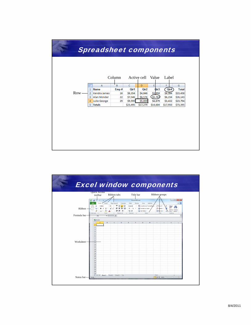
Label

Spreadsheet components

Row

Column ValueActive cell

Excel window components Quick Access

toolbar

Ribbon

Title bar Ribbon tabs

Formula bar

Worksheet

Status bar

Ribbon groups

8/4/2011

Enhanced ScreenTips

The Excel Help window

8/4/2011

Worksheet navigation methodsAction Result

Click a cell Selects that cell

Press arrow key Selects an adjacent cell

Press Tab Selects the cell one column to the right

Press Shift+Tab Selects the cell one column to the left

Press Ctrl+Home Selects cell A1

Press Ctrl+End Selects cell at intersection of last row and last column of data

continued

Worksheet navigation, continued

Action Result

Click scroll arrow Moves view of worksheet one row or column

Does not change the active cell

Click in scrollbar Moves view of worksheet one screen up, down, left, or right, depending on where you click

continued

8/4/2011

Worksheet navigation, continued

Action Result

Drag scroll box Moves view of worksheet quickly without changing the active cell

Press Ctrl+G (or choose Edit, Go To)

Opens dialog box where you can enter a cell address

Drag slider on zoom bar

Zooms in or out on current document

Spreadsheet with text and values

8/4/2011

Editing text and values• Select the cell and type the new data

• Click the formula bar, make the edits, and press Enter

• Double-click the cell to place the insertion point in it, make the desired edits, and press Enter

Using AutoFill1. Select the cell containing the value that starts the list or

series

2. Point to the fill handle until the pointer changes to a + symbol

3. Drag the fill handle over the adjacent cells that you want to fill

8/4/2011

Using AutoFill to fill a month series

Formulas• Perform calculations, such as adding, multiplying, and

averaging

• Begin with the = sign

• Use operators for calculations

8/4/2011

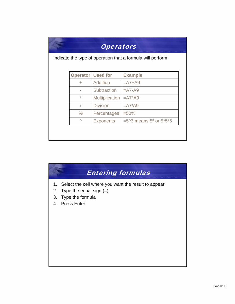
OperatorsIndicate the type of operation that a formula will perform

Operator Used for Example

+ Addition =A7+A9

- Subtraction =A7-A9

* Multiplication =A7*A9

/ Division =A7/A9

% Percentages =50%

^ Exponents =5^3 means 53 or 5*5*5

Entering formulas1. Select the cell where you want the result to appear

2. Type the equal sign (=)

3. Type the formula

4. Press Enter

8/4/2011

Entering cell references with mouse

1. Select a cell

2. Type =

3. Click the cell for which you want to enter a reference

4. Type the operator

5. Repeat Steps 3-4 until your formula is complete

6. Press Enter

Add an image to a worksheet1. Click the Insert tab

2. In the Illustrations group, click Picture

3. Navigate to the picture’s location, select the file, and click Insert

The picture appears in the worksheet, and the Picture Tools | Format tab is activated

4. Use the tools on the Format tab to modify the picture as necessary

8/4/2011

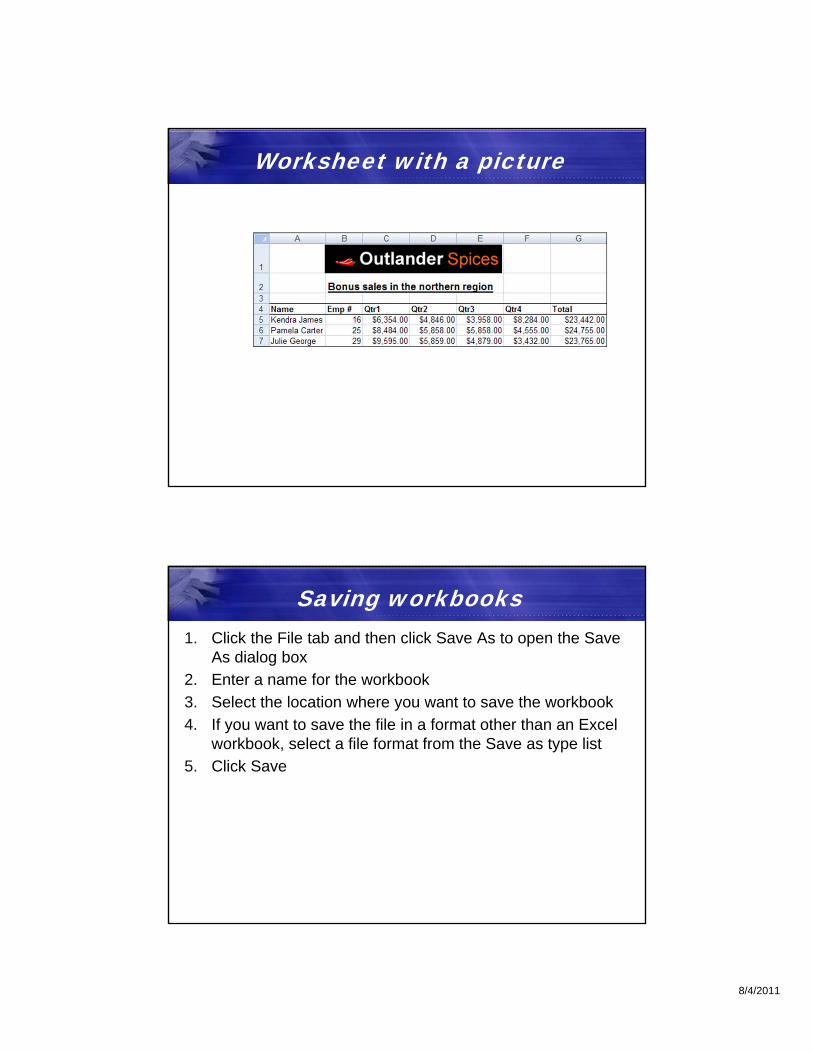
Worksheet with a picture

Saving workbooks1. Click the File tab and then click Save As to open the Save

As dialog box

2. Enter a name for the workbook

3. Select the location where you want to save the workbook

4. If you want to save the file in a format other than an Excel workbook, select a file format from the Save as type list

5. Click Save

8/4/2011

Saving a worksheet as a PDF1. With the worksheet open, click the File tab, and then click

Save As

2. Enter a name for the file (or use the current file name)

3. From the Save as type list, select PDF

4. Click Save

Excel converts the saved worksheet to a PDF file, and the current worksheet remains open in Excel

Moving data in worksheets1. Select the cell containing the data you want to move

2. Click the Home tab

3. In the Clipboard group, click Cut (or press Crtl+X)

4. Select the cell that you want to move the data to

5. In the Clipboard group, click Paste (or press Ctrl+V)

8/4/2011

Copying data1. Select the data you want to copy

2. In the Clipboard group, click Copy (or press Ctrl+C)

3. Select the destination cell for the data

4. Click Paste (or press Ctrl+V)

Moving data by dragging it1. Select the cell that contains the data you want to move

2. Point to the border of the cell until the pointer changes to a four-headed arrow

3. Drag the cell to where you want to move the data

4. Release the mouse button

8/4/2011

Copying data by dragging it1. Select the cell containing the data you want to copy

2. Point to the border of the cell until the pointer changes to a four-headed arrow

3. Press and hold Ctrl; the pointer displays a plus sign (+)

4. Drag to the destination cell, release the mouse button, and then release Ctrl

The Office Clipboard• Integrated across all Microsoft Office applications

• Expands the functionality of copy/paste and cut/paste

• Can hold multiple items—you’re not limited to pasting the most recently cut or copied item

• All items stored in the Office Clipboard are available to all open Microsoft Office applications

8/4/2011

Relative references• Cell reference

– Contains the row and column coordinates to identify a cell

• Relative cell reference

– Refers to other cells in a formula based on the location of the formula

– Automatically changes the references in a formula when it is copied

Absolute references• Don’t change when formulas are copied

• Are specified by using a $ sign

– $A$1

– $C$2

8/4/2011

Mixed references• Contain relative and absolute references

• Relative references change when you copy the formula

• Absolute references do not change

Inserting a range1. Click the first cell you want to select, and drag to the last

cell you want to select

2. In the Cells group on the Home tab, click Insert to display a menu

3. Choose Insert Cells to open the Insert dialog box

4. Specify whether you want to shift cells or insert an entire row or column, and click OK

8/4/2011

Inserting rows or columns1. Select the row or column where you want to insert a new

row or column

2. Do either of the following:

Right-click and choose Insert

Click Insert (in the Cells group) and then choose Insert Sheet Rows or Insert Sheet Columns

Deleting a range1. Select the range you want to delete

2. In the Cells group, click Delete(or right-click the selection and choose Delete)

3. Specify where to shift the adjacent cells

4. Click OK

8/4/2011

Function• Predefined formula that performs a specific type of

calculation=FUNCTIONNAME(ARGUMENT1,ARGUMENT2,…)

Arguments• Are the input values for a function

• Are enclosed in parentheses

• Can be numbers, text, cell addresses, ranges, and other functions

8/4/2011

Range reference• Specifies two or more cells

• Starts with the address of the first cell, followed by a colon (:) and the address of the last cell in the range

– A1:A4

– B4:H10

The Trace Error button• Appears when Excel suspects that a formula contains an

error

• Provides options for tracing possible errors in a formula

8/4/2011

Syntax errors

Inserting functions1. Select a cell

2. Click the Insert Function button on the formula bar

3. Select a function category and a function

4. Click OK

5. Specify the arguments

6. Click OK

8/4/2011

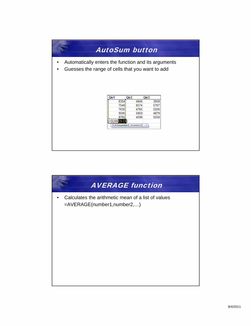
AutoSum button• Automatically enters the function and its arguments

• Guesses the range of cells that you want to add

AVERAGE function• Calculates the arithmetic mean of a list of values

=AVERAGE(number1,number2,…)

8/4/2011

MIN function• Returns the smallest number from a list of values

=MIN(number1,number2,…)

MAX function• Returns the largest number from a list of values

=MAX(number1,number2,…)

8/4/2011

COUNT function• Counts the number of cells in a range containing numeric

values

=COUNT(value1, value2, …)

Selecting a non-contiguous range

1. Select the first cell or range

2. While holding Ctrl, select any other cells or ranges you want to add to the selection

8/4/2011

Formatting cells1. Select the cell or range you want to format

2. Right-click the selection and choose Format Cells to open the Format Cells dialog box

3. Click the Font tab

4. Apply the desired formats, and click OK

Changing column widths• To resize a column:

– Drag the column border

– Double-click the column border

– Select a column, right-click, and specify the size in points

• Use the same methods to resize a row

8/4/2011

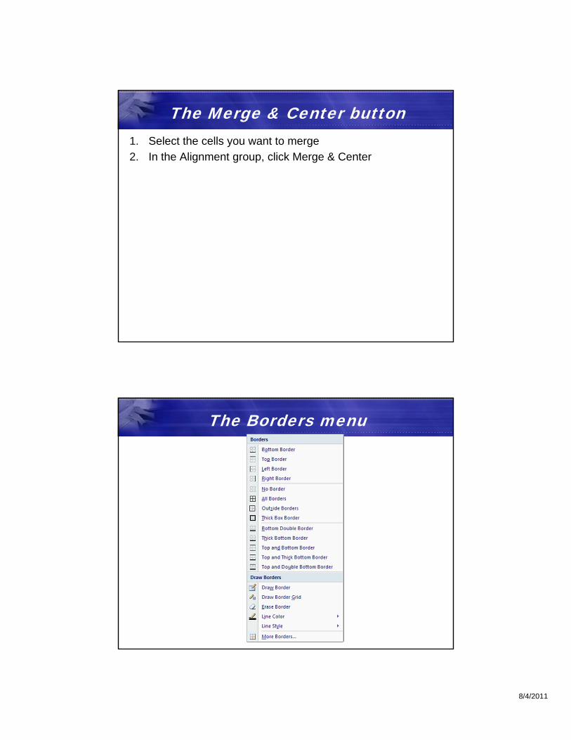
The Merge & Center button1. Select the cells you want to merge

2. In the Alignment group, click Merge & Center

The Borders menu

8/4/2011

Using the border-drawing pencil1. Click the Borders button

2. In the Borders gallery, click Draw Border, or select a line style and color

3. Drag where you want to apply a border

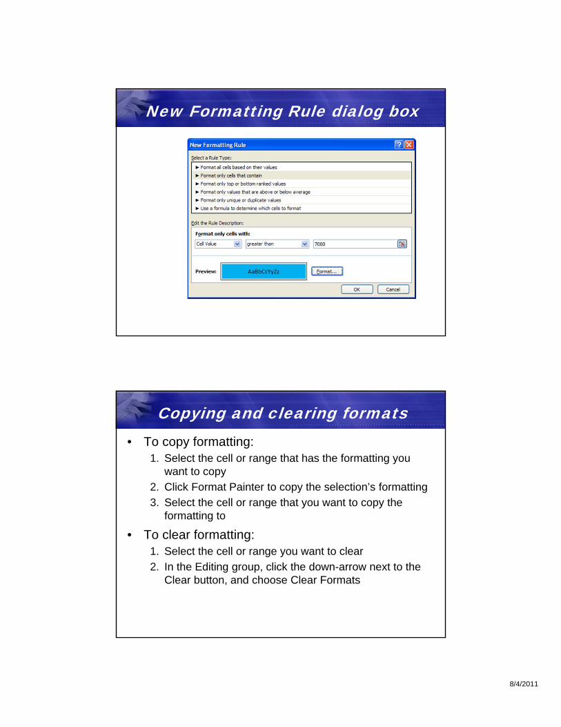
Number formatting

Currency Styles

Percent Style

Comma Style

Increase Decimal

Decrease Decimal

8/4/2011

The Number tab

Conditional Formatting menu

8/4/2011

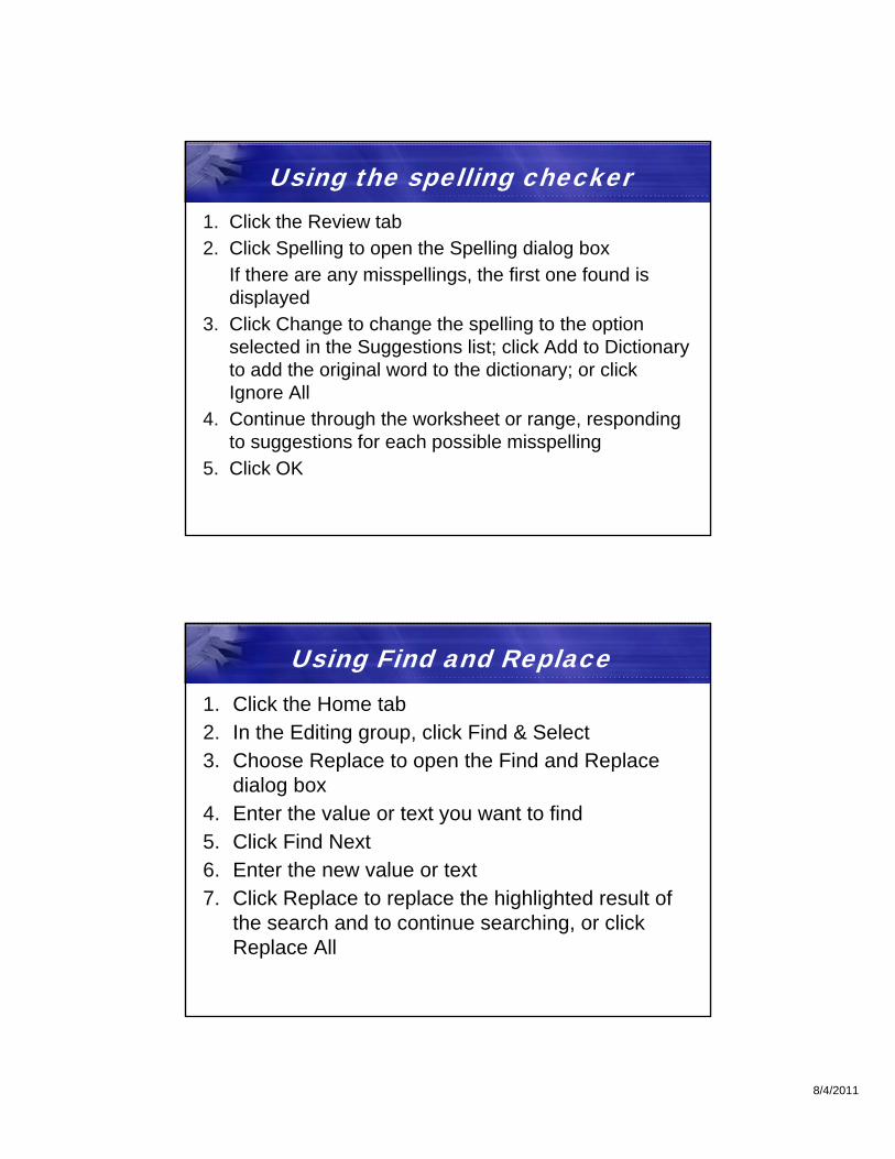
New Formatting Rule dialog box

Copying and clearing formats• To copy formatting:

1. Select the cell or range that has the formatting you want to copy

2. Click Format Painter to copy the selection’s formatting

3. Select the cell or range that you want to copy the formatting to

• To clear formatting:1. Select the cell or range you want to clear

2. In the Editing group, click the down-arrow next to the Clear button, and choose Clear Formats

8/4/2011

Applying a cell style1. Select a cell or range

2. In the Styles group, click Cell Styles

3. Move the pointer over the styles in the gallery—Live Preview shows how each style will affect the selected cell(s)

4. Click a style to select it

Applying a table format1. Select a cell or range2. In the Styles group, click Format As Table 3. Select a table format; the Format As Table dialog

box opens 4. Enter the range of the table and click OK; the

Table Tools | Design tab is activated 5. Use the Table Style Options and other groups on

the Ribbon as needed 6. Click anywhere in the worksheet to close the

Table Tools | Design tab

8/4/2011

Using the spelling checker1. Click the Review tab 2. Click Spelling to open the Spelling dialog box

If there are any misspellings, the first one found is displayed

3. Click Change to change the spelling to the option selected in the Suggestions list; click Add to Dictionary to add the original word to the dictionary; or click Ignore All

4. Continue through the worksheet or range, responding to suggestions for each possible misspelling

5. Click OK

Using Find and Replace1. Click the Home tab 2. In the Editing group, click Find & Select 3. Choose Replace to open the Find and Replace

dialog box 4. Enter the value or text you want to find 5. Click Find Next 6. Enter the new value or text 7. Click Replace to replace the highlighted result of

the search and to continue searching, or click Replace All

8/4/2011

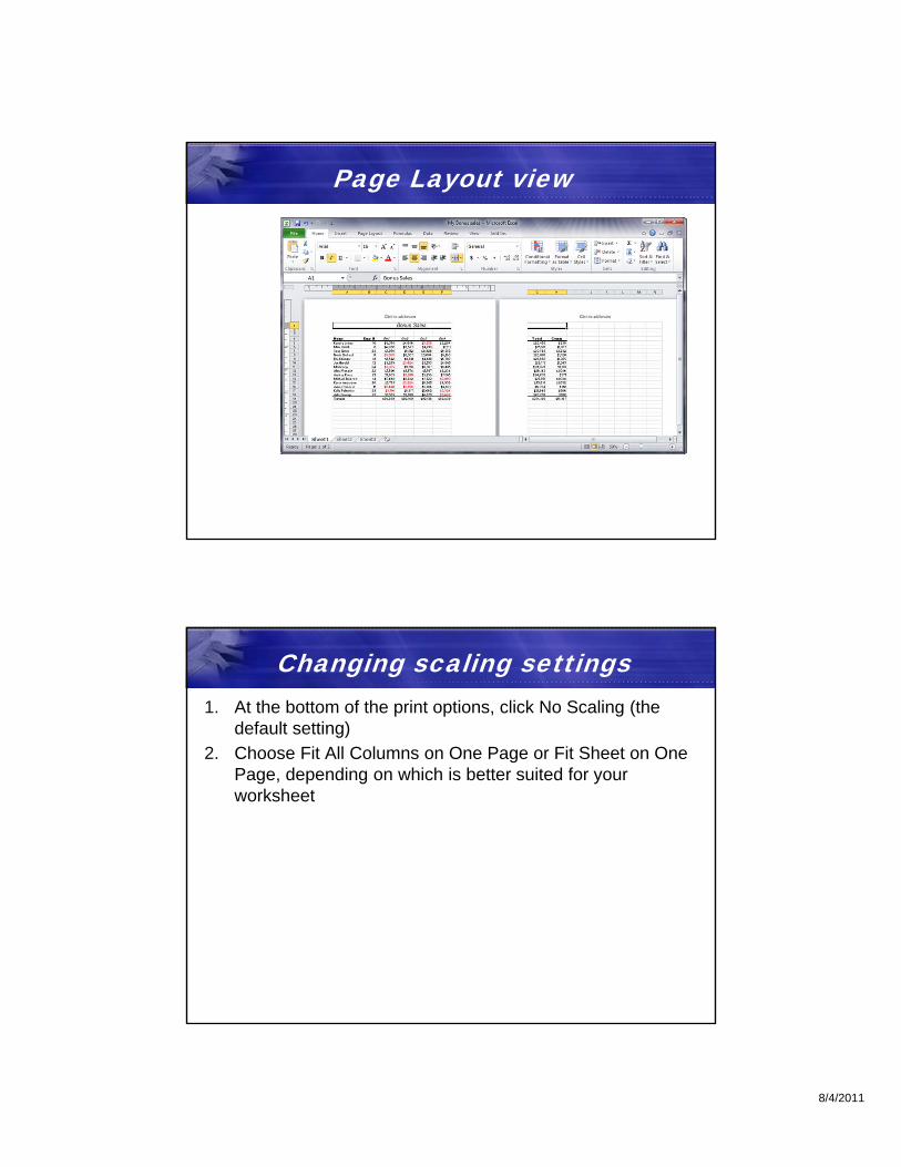
Page Layout view

Changing scaling settings1. At the bottom of the print options, click No Scaling (the

default setting)

2. Choose Fit All Columns on One Page or Fit Sheet on One Page, depending on which is better suited for your worksheet

8/4/2011

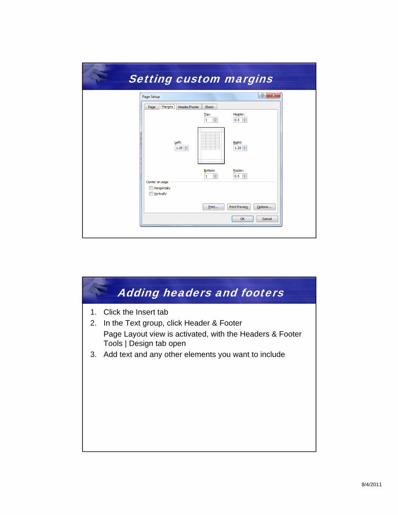
Setting custom margins

Adding headers and footers1. Click the Insert tab

2. In the Text group, click Header & Footer

Page Layout view is activated, with the Headers & Footer Tools | Design tab open

3. Add text and any other elements you want to include

8/4/2011

When you’re ready to print…1. Click the File tab

2. Click Print (or press Ctrl+P)

3. On the Print screen, select the printer you want to use, and select other settings such as page orientation, margins, and scaling

4. Click Print to print the worksheet

Printing a selection1. Select the range you want to print

2. Click the File tab and then click Print

3. Under Settings, click Print Active Sheets and then choose Print Selection

4. Click Print

8/4/2011

Creating a chart1. Select the headings and data you want in the chart

2. On the Insert tab, in the Charts group, click a chart type

3. Select a sub-type

4. Use the options on the Chart Tools tabs to format and customize the chart

5. Move the chart to the desired location on the worksheet

Chart elements

Value axis

Legend

Data series

Data point

Category axis

8/4/2011

Changing the chart type1. Select the chart

2. Under Chart Tools, click the Design tab and then click Change Chart Type

3. Select a chart type and a sub-type

4. Click OK

Adding axis labels1. Select the chart

2. Click the Layout tab

3. In the Labels group, click Axis Titles

4. Choose a horizontal or vertical axis title

8/4/2011

Freezing rows and/or columns1. Select the area you want to freeze:

– Row — Click a cell in the row below it

– Column — Click a cell in the column to its right

– Both row and column — Select a cell below and to the right of the row and column

2. Click the View tab

3. In the Window group, click Freeze Panes and then choose Freeze Panes

Splitting a worksheet into panes• To split horizontally:

1. Point to split box at top of vertical scrollbar

2. Drag down to where you want to split the worksheet

• To split vertically:

1. Point to split box to the right of horizontal scrollbar

2. Drag to the left

8/4/2011

Hiding a column1. Select a column heading or row heading, or drag across

multiple column or row headings

2. Right-click the selection

3. Choose Hide

Unhiding columns1. Select the columns on both sides of the hidden row(s) or

column(s)

2. Click the Home tab

3. In the Cells group, click Format and choose Hide & Unhide, Unhide Columns

8/4/2011

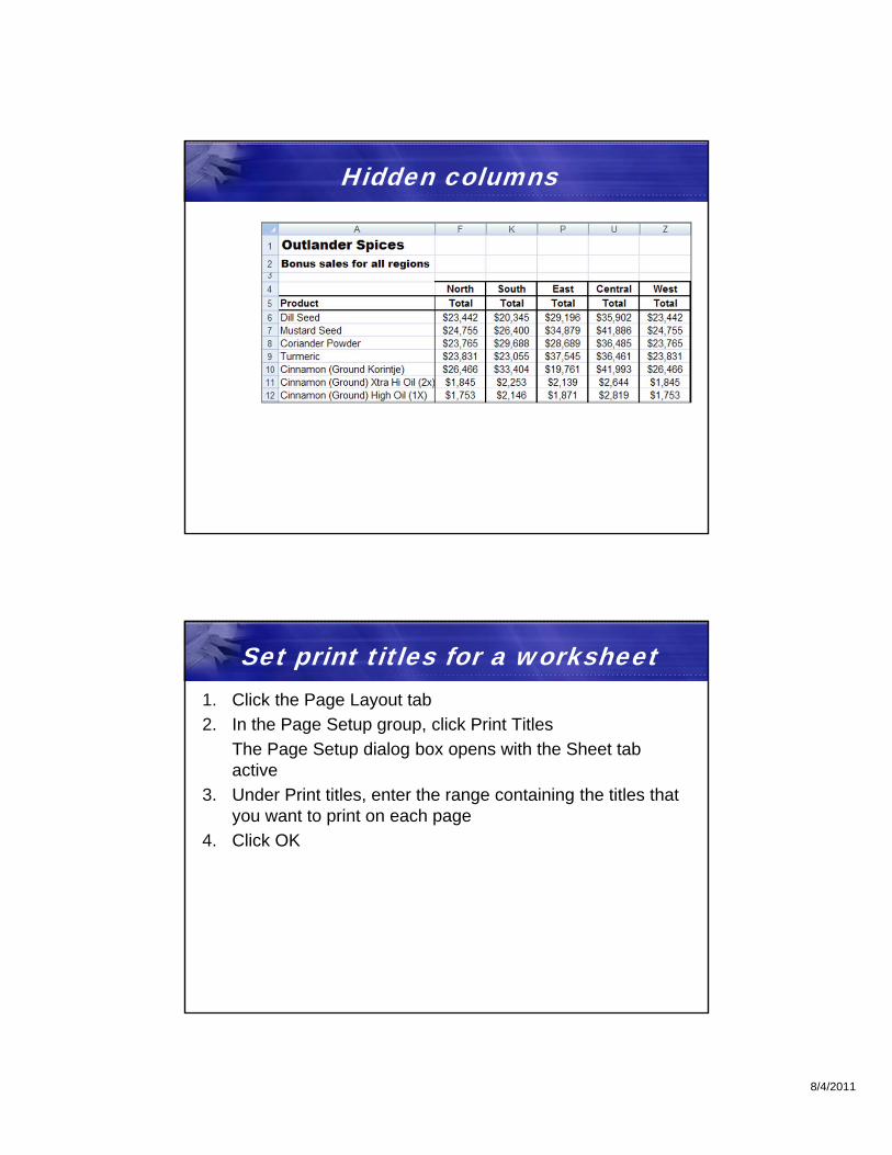
Hidden columns

Set print titles for a worksheet1. Click the Page Layout tab

2. In the Page Setup group, click Print Titles

The Page Setup dialog box opens with the Sheet tab active

3. Under Print titles, enter the range containing the titles that you want to print on each page

4. Click OK

8/4/2011

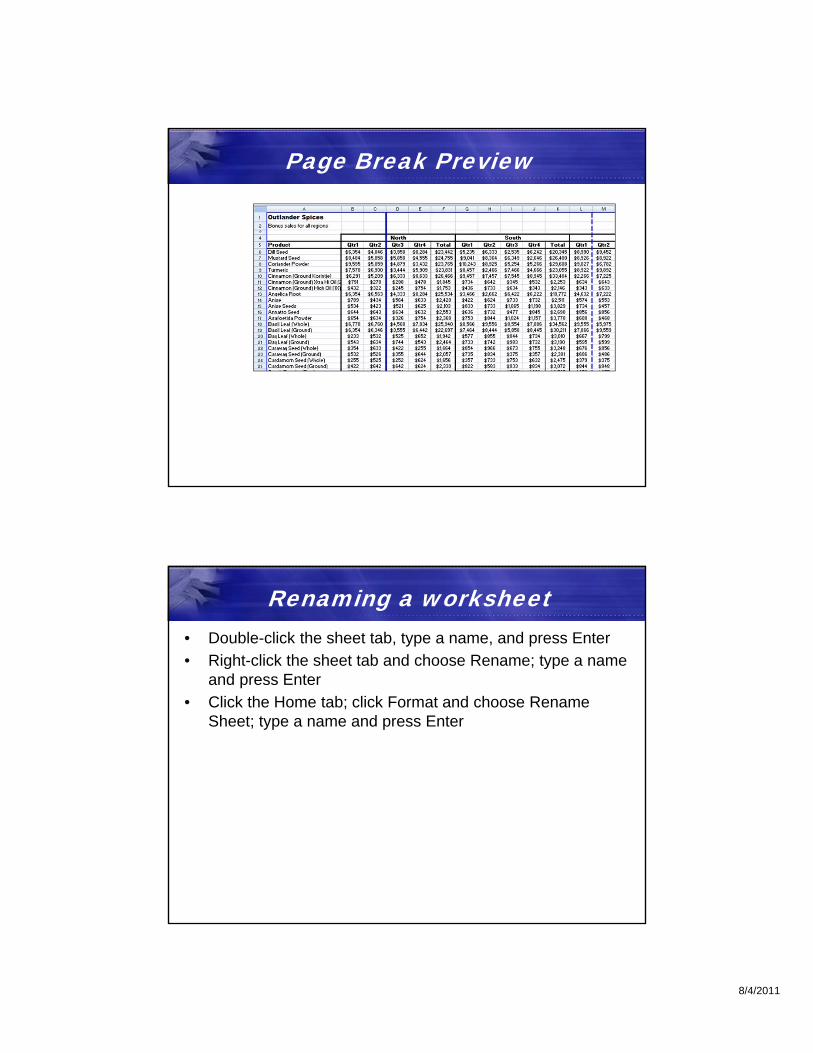
Page Break Preview

Renaming a worksheet• Double-click the sheet tab, type a name, and press Enter

• Right-click the sheet tab and choose Rename; type a name and press Enter

• Click the Home tab; click Format and choose Rename Sheet; type a name and press Enter

8/4/2011

Formatting worksheet tabs1. Right-click a worksheet tab to display a shortcut menu

2. Choose Tab Color to open a color palette

3. Select the color you want to apply; select another tab to see the results

Inserting a worksheet• Click the Insert Worksheet button (to the right of the current

tabs)

• Press Shift+F11

• In the Cells group (Home tab), click the Insert button’s down-arrow and choose Insert Sheet

• Right-click a worksheet tab, choose Insert, select Worksheet, and click OK

8/4/2011

Moving a worksheet1. In the Cells group, click Format and choose Move or Copy

Sheet

2. Select a new location for the worksheet from the To book list or the Before sheet list

3. If you want to copy the sheet (rather than move it), check “Create a copy”

4. Click OK

Deleting a worksheet• Right-click the sheet tab and choose Delete

• In the Cells group, click the Delete button’s down-arrow and choose Delete Sheet

8/4/2011

Printing multiple worksheets1. Press Ctrl and click the tabs to select the worksheets you

want to print

2. Click the File tab and click Print to display print options and preview window

3. Click Print to print the selected worksheets