colloids and pulsing force ﬁelds: eﬀects of spacing mismatch

Facolta di Scienze e Tecnologie

Laurea Magistrale in Fisica

Colloids and pulsing force fields:effects of spacing mismatch

Relatore: Prof. Nicola Manini

Correlatore: Dr. Andrea Vanossi

Stella Valentina Paronuzzi Ticco

Matricola n◦ 809466

A.A. 2012/2013

Codice PACS: 82.70.dD

Contents

1 Introduction 4

1.1 The Frenkel-Kontorova Model . . . . . . . . . . . . . . . . . . . . 4

1.1.1 The Aubry Transition . . . . . . . . . . . . . . . . . . . . 6

1.1.2 Kinks and Antikinks . . . . . . . . . . . . . . . . . . . . . 7

1.2 Shapiro Steps . . . . . . . . . . . . . . . . . . . . . . . . . . . . . 9

1.3 Colloids: the Stuttgart Experiment . . . . . . . . . . . . . . . . . 12

2 The Model 14

3 Fixed Density 20

3.1 Commensurate Systems . . . . . . . . . . . . . . . . . . . . . . . 20

3.2 Incommensurate Systems . . . . . . . . . . . . . . . . . . . . . . . 25

3.2.1 Subharmonic Antisolitons . . . . . . . . . . . . . . . . . . 27

3.2.2 The Overall Corrugation Amplitude . . . . . . . . . . . . . 31

4 Inhomogeneous Layer 36

4.0.3 Evaluation of vcm . . . . . . . . . . . . . . . . . . . . . . . 37

4.1 Full matching . . . . . . . . . . . . . . . . . . . . . . . . . . . . . 38

4.2 Lattice-mismatched Sistems . . . . . . . . . . . . . . . . . . . . . 41

4.2.1 alas/acoll ≃ 0.93; V0 = 0.5; ∆0 = 70%V0 . . . . . . . . . . . 41

4.2.2 alas/acoll = 0.9; V0 = 0.5; ∆0 = 100%V0 . . . . . . . . . . . 44

4.2.3 alas = 0.9; V0 = 1; ∆0 = 100%V0 . . . . . . . . . . . . . . . 47

5 Discussion and Conclusions 50

Bibliography . . . . . . . . . . . . . . . . . . . . . . . . . . . . . . . . 52

3

Chapter 1

Introduction

Nonlinear systems driven far from equilibrium can show widely intriguing pat-

terns of varied and often unexpected dynamical behavior. As a result more and

more studies every day address the field of nonequilibrium dynamics of system

with many degrees of freedom. An especially interesting case is that of many

identical interacting particles which may get trapped in some external potential,

as often happens in solid-state physics. It has frequently been shown that even

simple, low-dimensional, phenomenological models of friction can help in unrav-

elling experimental results on nanoscale tribology, when they capture the main

features of the complex dynamics involved.

As a preliminary introduction we sketch a simple yet fundamental model:

the Frenkel-Kontorova model. Describing the dissipative dynamics of a chain of

interacting particles that slides over a rigid periodic substrate potential, under

the application of an external driving force, this many-body model exhibits the

right features in order to be the true key for the understanding of the atomic

processes occurring at the interface of two materials in relative motion.

1.1 The Frenkel-Kontorova Model

A simple model that describes the dynamics of a chain of particles interacting with

the nearest neighbors in the presence of an external periodic potential was firstly

mentioned by Prandtl [1] and Dehlinger [2]. This model was then independently

[3] introduced by Frenkel and Kontorova [4].

The original Frenkel-Kontorova model (FK in the following) is a one-dimensional

harmonic chain of particles put on a periodic (sinusoida) substrate (Fig. 1.1). The

4

CHAPTER 1. INTRODUCTION 5

Figure 1.1: Schematic presentation of the Frenkel-Kontorova model: A chain

of particles interacting via harmonic springs with elastic coupling K subjected to

the action of an external periodic potential with period as

Hamiltonian is given by

H =N∑

n=1

{

K

2(xn+1 − xn − a0)

2 − V0 cos

(

2πxnas

)}

, (1.1)

Where xn denotes the position of the n-th particle. Nearest-neighbor particles are

connected to each other by Hookian springs of strength K, as described by the

first term in the Hamiltonian, where a0 is the natural spacing between particles.

The 2nd term describes the interaction of the chain with the sinusoidal substrate

potential, with height 2V0 and period as.

An essential feature of this model is the competition arising between the

natural spacing a0 imposed by the spring stiffness and the substrate potential

period which tends to keep particles a distance as away; it is convenient to de-

fine a parameter that describes this characteristic ratio: the winding number

f = a0/as. This competition, often referred to as frustration, can result in a

fascinating complexity of spatially modulated structures. Of very high interest is

the incommensurate structure, generated when the substrate periodicity and the

natural chain spacing (written as as = L/M and a0 = L/N , being M and N the

number of potential well and the number of particle along the chain respectively)

are such that, in the infinite size limit L→ ∞, f equals an irrational number. It

can be shown that at fixed V0, the FK model undergoes a transition (the Aubry

transition [6]) at a value Kc of the interatomic interaction strength, that depends

strongly on f . In particular it has been proved that when f assumes the golden

mean value (1 +√5)/2, Kc(f) takes the lowest possible value.

This transition consists in the following: when K > Kc(f) there exists

a continuum of ground states that can be reached by the chain through non-

rigid displacements of its atoms with no energy cost (superlubric regime); when

K < Kc(f) the atoms are pinned in the neighborhood of the potential well and

a finite amount of energy must be spent to move them.


(a) A continuous hull function describes

an incommensurate ground state when K

is above the Aubry transition. Here f =

144/233 is used as a good approximation

to the golden mean (√5 + 1)/2; Gf (x) is

represented mod 1.

(b) Incommensurate ground states of the

standard Frenkel-Kontorova model are

described by a discontinuous hull func-

tion when K is below the Aubry transi-

tion point.

Figure 1.2: Analytic and non analytic behavior of the hull function for values of

K below and above the critical point, respectively. (Figures taken from Ref. [18]).

1.1.1 The Aubry Transition

A remarkable feature of the FK model is that mathematically rigorous analysis

of the low lying states is possible, based on the fact that configuration of the

energy minima of the system satisfies a recursion relation, which is identical to

the so-called standard map well known in dynamical system [9]. Focusing on the

incommensurate ground states, it can be shown [5] that they are characterized

by the existence of a hull function Gf (x), giving the ground state configuration,

which has the following properties:

• is strictly increasing

• is step periodic, i.e.

Gf (x+ 1) = Gf (x) + 1. (1.2)

• If Gf (x) is a continuous function, for any real number α the configuration

{xj}, defined as

xj = Gf (jf + α), (1.3)

is a ground state configuration; vice versa: any ground state configuration

with winding number f is of the form (1.3).

• Gf (x) is unique.


Gf (x) (meta)stable states

K > Kc(f) analytic only the ground state

K < Kc(f) non-analytic, infinitely many

with infinitely many discontinuities metastable states [11]

Table 1.1: Properties of the hull function and of the low lying states across the

Aubry transition.

It is the critical valueKc(f) that marks the border between continuous (Fig. 1.2 a)

and non-analytic ground states (Fig. 1.2 b ): in Table 1.1 we summarize the basic

feature of the transition from analyticity to non analyticity of the hull function

(from which the name transition by breaking of analyticity given by Aubry).

From a physical point of view the fact that the hull function is continuous

means that the ground state is sliding : starting from a ground state one can find

a continuum of states with exactly the same energy by varying α; they are all

related to each other by some continuous displacement of the particles in real

space and no external force is needed to slide the whole system — frictionless or

superlubric state [8]. Such a frictionless state persists until K crosses the critical

value: for K < Kc(f), discontinuous points appear in the hull function Gf (x)

(Fig. 1.2 b )). This means that a variation of α requires discontinuous movements

of the particles in the real space. As a consequence the ground states are no longer

connected to each other by sliding: the system prepared in one ground state has

to go over some higher energy state (energy barrier) to reach another ground

state. Thus the system is jammed, and some finite strength of external force

greater than a certain minimum frictional force fyield(K) ∝ (Kc−K)γ is required

to be applied for the system to depin and start to move.

So it can be said that the Aubry transition is a ’frictional transition’ describ-

ing the transition of the system from a superlubric, freely sliding phase character-

izing the rigid chainK > KC to a soft-chain jammed (pinned) phase characterized

by nonzero static friction.

1.1.2 Kinks and Antikinks

As we have already underlined an essential feature of the f 6= 1 FK model is

the competition between the interparticle interaction and the substrate periodic

potential: the former favoring a uniform separation between particles, the lat-

ter tending to pin atoms position to the bottom of potential wells, the whole

mechanism inducing frustration in the system.


(a) Sketch of a kink in a chain of particles

(pink dots) on a one-dimensional substrate

potential. A kink is formed when two par-

ticles of the chain entrapped in the same

potential well, forming a local compression.

(b) Sketch of an antikink, corresponding to

a local expansion of the chain. Note that

an antikink will propagate in a direction

reversed with respect to the force F .

Figure 1.3: The ease with which a (anti)kink moves, compared to regular par-

ticles sitting at the corrugation energy minima, provides an efficient mechanism

for mass transport along the chain in the (opposite) direction of an externally

applied force F .

Despite the extreme simplification that are made in the FK model com-

pared to a real system, there is one important feature, beside many others, of

course, which can explain why this model attracted so much attention: in the

continuum-limit approximation the model reduces to the exactly integrable sine-

Gordon equation, which allows exact solutions describing different types of non-

linear waves and their interactions. The sine-Gordon system represents one of the

rare examples of a model for which almost everything is known about nonlinear

excitations. This equation:

∂2x

∂t2− ∂2x

∂x2+ sin(x) = 0 (1.4)

where x is a new introduced variable obtained by changing n → x = nas, de-

scribes different types of elementary excitations: phonons, kinks, breathers. Using

the language of the sine-Gordon quasi-particles as weakly interacting nonlinear

excitations can be very useful in understanding the nonlinear dynamics of the

FK model. In the context of friction the most important among these excitations

is the kink. Let us consider the simplest system that can be made beyond a

completely commensurate one: a chain with a number N of atoms on a substrate

potential with N−1 minima. Its ground state contains a kink, Fig.1.3 (a), namely

a configuration with one extra particle inserted in the chain and deforming the

otherwise commensurate structure. If we let the system relax we end up having

a local compression in the chain. In terms of the sine-Gordon model, a kink is


represented by a region where the phase variable jumps by 2π.

The reason why this kind of excitation is so important is that it can move

along the chain much more easily than single atoms themselves. The energy bar-

rier (Perls-Nabarro barrier) that a kink has to overcome1 in order to slide by one

substrate lattice spacing is always smaller (often much smaller) than the ampli-

tude of the substrate potential. Because the kink stands for an extra particle, its

motion provides a valid and efficient method of mass transport along the chain.

The higher the kinks concentration the larger the chain mobility (but also con-

ductivity, diffusivity, and all the other transport properties). This argumentation

holds symmetrically for antikinks (Fig.1.3 b), that can be seen as vacancies.

Many relevant generalizations of the FK model have been proposed so far in

the literature to cover a broad class of physically interesting phenomena [3]. For

describing realistic physical systems (such as, for example, atoms adsorbed on a

crystal surface), different types of anharmonicity can be introduced suitably in

the interatomic potential of the chain. In a similar way, it is sometimes helpful

to consider substrate potentials, which may vary substantially from the simple

sinusoidal shape assumed in the standard FK model, with a possible consequent

drastic change in the statics and dynamics occurring between the surfaces. An

important and more realistic generalization of the standard FK chain with rel-

evant consequences for the resulting tribological properties (critical exponents,

scaling of friction force with system size, mechanisms of depinning, etc) is to

increase the dimensionality of the model.

To the purpose of the present work, the main take-away message of FK

physic is that as a function of the corrugation amplitude we should expect a non-

trivial behavior of the low-lying states which has fundamental consequences on

the sliding physics when an external force attempts to make the system slide.

1.2 Shapiro Steps

In 1962 it was realized [12] that in the presence of microwaves, the Josephson

current in a Josephson junction2 might be a non vanishing quantity for special

values of the DC-voltage. The first detection of this phenomenon was made

by Shapiro a year later [13] in an experiment where a clear step structure (later

named a Shapiro-step structure) was found in the I-V curve of the DC components

of the electric response of the junction (Fig. 1.4).

1The Perls-Nabarro barrier in a consequence of the discrete nature of the FK model: in the

continuum sine-Gordon limit no PN barrier is present [18].2A Josephson junction consists of two superconductors separated by a thin insulating barrier

which electrons can tunnel through.


Figure 1.4: Tunneling current vs voltage characteristics displayed on an oscil-

loscope in a sample of Al/Al2O3/Sn at about 0.9K with microwave power at 9300

Hz (A) and 24850 Hz (B). From the original 1963 Shapiro paper [13].

The equation for the current in a Josephson junction is

J(t) = J0 sin(δ) with∂δ

∂t=

2eV

~. (1.5)

It is straightforward to derive [14]. Here δ = φ1 − φ2 is the phase difference be-

tween the wave functions ψ1 and ψ2 of the superconducting state in the left and

in the right superconductor, respectively. The current density J is called Joseph-

son current or supercurrent. This strongly non-linear current-voltage behavior is

at the origin of many different physical phenomena like the DC Josephson effect

and the AC Josephson effect. Let us focus on the former: when a DC voltage V0(or a DC current larger than J0) is applied to the junction, the phase difference

rotates at an angular frequency:

ω0 =2eV0~

(1.6)

so that according to Eq. (1.2) the current

J(t) = J0 sin(ω0t). (1.7)

The Josephson current will oscillate at a frequency ω0 = V0 · 483.6 GHz/mV.

This high frequency means that the detection of this current could become very

difficult due to the damping caused by junction capacitive and resistive properties.


In practice one measures an average zero current density, and the oscillating

current results in a weak emission of electromagnetic radiation in the microwave

spectrum3.

This AC effect may also be observed in a somewhat easier, although indi-

rect, method. If a small high frequency AC voltage oscillating at frequency ω is

superimposed to the DC voltage applied across the junction, then there will be

discrete DC voltage levels where the supercurrent becomes finite, and does not

oscillate. Eventually the Josephson current becomes:

J(t) = J0

[

sin(δ0 + ω0t) +2eV

~ωsin(ωt) · cos(δ0 + ωt)

]

(1.8)

The first term again is an oscillating current which averages to zero; however if

mω = ω0 (1.9)

with m an integer, the second term becomes finite, containing terms like sin2(ωt)

which are finite in time average: the DC current will not be a vanishing quantity

jumping suddenly at a nonzero value when the potential is an integer multiple of

~ω0/2e. These structures are called Shapiro spikes.

Unfortunately in a real experiment it is very difficult to voltage-bias a junc-

tion: the impedance of the junction is so small that, unless special precautions

are taken, the voltage source effectively acts like a current source. The equations

for a current-biased junction are much more difficult to solve and can only be

dealt with numerically. However the result is not difficult to appreciate. Instead

of getting current spikes when the resonant condition is met, steps4 at the voltage

level itself are found: the Shapiro steps (Fig. 1.4).

The Shapiro spikes and steps can be interpreted as mode-locking phenomena

of the Josephson junction. When the average voltage of the source is close to an

integer multiple of the frequency of the oscillating source divided by 2e/~, the

Josephson junction tunes in with the source.

Step-like structures arise in many systems in which two competing frequency

scales are present. The system we are going to study is composed by an ensem-

ble of colloidal particles being dragged by an external force over a periodically

oscillating potential. When a time-oscillating external perturbation acts on this

3The phenomenon can be understood in term of energy conservation: if a Cooper pair

tunnels between the two superconductors, where the energy levels differ by 2eV0, to get into

the condensate state a photon must be emitted.4It has been shown that the positive steps correspond to a tunnelling pair with photon

emission, and the negative going steps correspond to a tunnelling electron pair with photon

absorption.


system the frequency ν of this oscillation and the characteristic frequency ν0 of

the motion over the periodic substrate potential driven by the average force can

give rise to Shapiro steps, which are the main focus of our investigation.

1.3 Colloids: the Stuttgart Experiment

In 2011 T. Bohlein, J. Mikhael and C. Bechinger performed a pioneering ex-

periment, in which charged colloidal particles (polystyrene spheres with radius

R = 1.95 µm) were driven across a periodic potential generated by a light inter-

ference pattern. The colloidal particles repeal each other and are confined in a 2D

region, so that they tend to form a triangular lattice. The interference pattern

can be treated in such a way that the periodic potential it produces is either

commensurate or incommensurate to the colloidal lattice.

The really innovative feature of this work is that the actual 2D motion of

every individual particle can be observed in time during sliding, providing an

unprecedented real-time insight into the basic dynamical mechanisms at play,

hitherto restricted to the ideal world of MD simulations. In their experiment

Bohlein and co-workers could observe [15] the formation of topological solitons

(Fig. 1.3) the kinks and antikinks of the FK model. These excitations, believed

to dominate the frictional properties at atomic length scale providing an efficient

mechanism for mass transport, were observed here for the first time in a sliding

friction experiment. Figure 1.5 illustrates the soliton mechanism as observed in

experiment.

To our knowledge no experiment yet has achieved to detect Shapiro-step

structures in colloid dynamics. Simulation works on this topic have been pub-

lished [16], focusing, however, on idealized conditions.

In the present work we study the feasibility of the investigation of Shapiro

steps under experimentally realistic conditions. More specifically we mimic an

ensemble of repulsive colloidal particles in a periodic potential (generated by laser

light interference), oscillating in space and even in time. Using classical molecular

dynamic we monitor the behavior of the particles themselves under the action of a

DC force. As a function of this force the headway velocity of the colloidal particles

can turn out ’quantized’ in ’terraces’ independent of the applied force (namely

Shapiro steps). Our aim here is to characterize those step structures in relation

to the presence or absence of solitonic defects due to the mismatch between the

colloidal lattice spacing and the force field. In particular, we intend to predict

under which experimental conditions these Shapiro steps are best observed.


Figure 1.5: The propagation of a soliton (darker green) over a periodic lattice

marching the substrate, as observed in Stuttgart experiment [15]. A force of F =

40 fN driving all colloids to the right, the time interval between successive snapshot

is 13 s.

Chapter 2

The Model

We describe charged colloidal particles as classical point-like objects, whose dy-

namics is affected by the action of external forces, the mutual repulsion, and the

interaction with the viscous solution in which they are immersed.

The equation of motion for the j-th particle is

mrj(t) + η(rj(t)− vdx) = −∇rj(U2 + Uext) + fj(t) , (2.1)

where rj is a two-dimensional position vector of the j-th colloid, η is the friction

coefficient determined by the effective viscosity of the fluid in which the colloids

are immersed, and vd is the fluid drift velocity, giving rise to the Stokes driving

force Fext = ηvd, acting on all colloidal particles. U2 is the two-body inter-particle

potential; Uext is the external potential, which is time-dependent: in this work

we will study the behavior of our system under periodic oscillation of Uext with

different amplitude and frequencies. In our system colloidal particles interact

with the fluid, with which they are at - or very close to - thermal equilibrium.

The fluid involves a huge number of degrees of freedom varying rapidly on the

colloidal particles’ timescale. We simplify this interaction, adopting a Langevin

approach, substituting the fluid with two terms in the equation of motion (2.1),

that describes the Brownian motion of the colloidal particles in our viscous so-

lution: the viscous friction term η(rj(t) − vdx), and the term fj(t), which is a

suitable two-components Gaussian random force [21]. This term stands for the

random collisions between colloidal and fluid particles, due to the thermal motion

of the fluid, and inducing Brownian motion. In the present work we will initially

focus only on zero-temperature simulations, thus for the time being the random

force will be set to zero.

For the slow motion (vd ≃ 1 µm s−1) of a colloidal particle in the liquid

the inertial term can be neglected, and a diffusive motion can safely be assumed,

with an appropriate choice of η (in our work η = 28 expressed in model units,

14

CHAPTER 2. THE MODEL 15

given in Table 2.1).

The 2-body interaction potential is

U2 =N∑

j<j′

V (|rj − rj′ |) , (2.2)

and the screened Coulomb repulsion V varies with inter-particle distance as a

Yukawa-type potential:

V (r) =Q

rexp(−r/λD) . (2.3)

The above expression holds only for separation r larger than the diameter ≃3.9 µm of a colloidal particle, where an additional hard-core repulsion sets in.

Typical nearest-neighbor separations at which colloids settle in experiments are

r ≃ 5.7 µm ≃ 30λD [15]. Due to the comparably short Debye length λD, when

two colloids happen to approach just a little closer than that, the violent expo-

nential increase of V (r) pushes them apart far before the hard-core repulsion sets

in. Thus explicit inclusion of the hard-core term is unnecessary, as it would cause

no change to the trajectories. Due to the moderate volume fraction occupied

by the colloidal particles in the solution and the adiabatically slow motions oc-

curring near a rigid surface moving at vd(the cell bottom), it is also appropriate

to neglect hydrodynamic forces [22], which would become relevant only at much

denser/faster regimes.

The potential in Eq. (2.3) is clearly a short-range potential. Thus, to reduce

computational time, we neglect it starting from a certain cutoff distance, which

is chosen to guarantee that the difference between the approximate (cutoffed)

potential and the exact one is extremely small. This cutoff distance is:

rcut = CλD , (2.4)

where C is the cutoff factor, that is set to 100 in agreement with the study carried

out in Ref. [23], so that the exponential term in Eq. (2.3) equals exp(−100) ≃4×10−44. In order to avoid discontinuities in the potential and in the force, which

could induce important errors during the numerical integration of Eq. (2.3), the

original interparticle potential is shifted, so that it vanishes with its derivative at

rcut. So the implemented potential is:

V (r) =

[

Q

rexp(−r/λD) + φ(r)

]

θ(rcut − r) , (2.5)

where θ(r) is the Heaviside step function, and φ(r) is the linear function by which

the original potential is shifted:

φ(r) = r

(

Q

r2cut+

Q

λDrcut

)

exp(−rcut/λD) −(

2Q

rcut+

Q

λD

)

exp(−rcut/λD) . (2.6)


This originates a constant additional force between the particles, but, for large

enough rcut, this term has a negligible effect due to the exponential factor in

Eq. (2.4).

The 1-body external potential energy

Uext =N∑

j

Vext(rj) , (2.7)

is induced by the interaction of the colloidal particles with a laser field. In ex-

periment Vext(r) and can be shaped with substantial freedom. We simulate the

experimental laser interference pattern adopting the following spatial variation:

Vext(r) = Ac[1−G(r)] + V0G(r)W (r) , (2.8)

where

G(r) = exp

(

−|r|22σ2

)

, (2.9)

is an unnormalized Gaussian of (large) width σ, accounting for the overall inten-

sity envelope of the laser beam, and

W (r) = Wn(r) = − 1

n2

∣

∣

∣

∣

∣

n−1∑

l=0

exp(ikl · r)∣

∣

∣

∣

∣

2

, (2.10)

is a periodic (for n = 2,3,4, or 6) or quasi-periodic potential of n-fold symme-

try [24] produced by the interference of n laser beams, representing the substrate

corrugation. The appropriate 2D interference pattern is realized by taking

kl =cnπ

alas

[

cos

(

2πl

n+ αn

)

, sin

(

2πl

n+ αn

)]

. (2.11)

The numerical constants cn are chosen in order to match the potential lattice

spacing to the laser interference periodicity alas, and αn are chosen so that one

of the primitive vectors of the periodic potential Wn(r) is directed along the x

axis [25]. In the present work, we adopt a 3-fold symmetry pattern, thus n = 3,

like for the colloidal lattice. In this case, we use c3 = 4/3 and α3 = 0.

Expanding the absolute value and rearranging the expression with some

trigonometric relations we obtain :

W (r) = W3(r) = −1

9

[

3 + 2 cos

(

4πry√3 alas

)

+ 4 cos

(

2πry√3 alas

)

cos

(

2πrxalas

)]

,

(2.12)

which is the potential depicted in Fig. 2.1. If we fix ry so that a path along the

rx direction crosses perpendicularly the saddle points this path also goes through


Figure 2.1: The triangular-symmetry corrugated potential energy profile

W (x, y) = W3(x, y) as a function of position. Observe the minima at energy

(in units of V0) −1, the saddle points at energy −19and the maxima at energy 0.

The resulting lowest-energy barrier in the x-direction thus equals 89.

-1 0 1x/alas

-1

-0.8

-0.6

-0.4

-0.2

0

W3(x

,0)

Figure 2.2: The 1-dimensional curve obtained setting y = 0 in W3(x, y), as a

function of x.


Physical quantity Model expression Typical value

Length acoll 5.7 µm

Force F0 = 9Fs1/(8π) 18 fN

Viscosity coefficient η 6.3× 10−8 kg/s

Energy F0 acoll 1.0× 10−19 J

Time ηa2coll/V0 20 s

Mass η2acoll/F0 1.3× 10−6 kg

Velocity F0/η 0.284 µm/s

Power F 20 /η 5.1× 10−21 W

Table 2.1: Basic units for various quantities in our model, with typical values

appropriate for the setup by Bohlein et al. [15].

the minima, and we obtain the 1-dimensional path where the barrier from one

minimum to the next is lowest. For example we can choose ry = 0, so we have:

W (rx, 0) = −1

9

[

5 + 4 cos

(

2πrxalas

)]

, (2.13)

which is the curve shown in Fig. 2.2, where we can see that the potential difference

between a minimum and a saddle point is 89V0. This barrier is relevant near the

center of the cell, where the prefactor G(r) ≃ 1. The static friction force for an

isolated colloid, i.e. the minimum force that a single colloid requires in order to

slide in this 1-dimensional potential is

Fs1 =8πV09alas

=8π

9F0 . (2.14)

The two positive amplitudes Ac and V0 set, respectively, the intensity of

the overall potential confining the colloids near the simulation-cell center and the

intensity of the corrugated, spatially oscillating term. Both of them are controlled

by the same overall Gaussian intensity modulation, Eq. (2.8), consistently with

experiments [15]. The simulations are carried out in dimensionless units, defined

in terms of the physical quantities reported in Table 2.1. From now on we will

adopt these units.

Shapiro steps are investigated by modulating the periodic potential ampli-

tude sinusoidally in time. Specifically, Eq. (2.8) is modified to

Vext(r, t) = Ac[1−G(r)] + [V0 +∆0 sin(ωt)] G(r)W (r) , (2.15)

where ∆0 is the potential oscillation amplitude, while ω/2π is the frequency ν

with which the potential oscillates. This modulation will lock to the oscillation


generated from the dragging of the colloids over the periodic potential with a DC

force, giving rise to Shapiro step structures in the rate with which the velocity

varies with force. The frequency is not to be chosen too high since we are dealing

with an overdamped system, as explained in the next chapter.

Chapter 3

Fixed Density

The aim of the present work is to simulate an open system composed by a num-

ber of particles sufficient to predict reliably the conditions for the occurrence of

Shapiro steps in experimentally realistic setups. As a preliminary stage of this

investigation, it is desirable to test this physics in a configuration where the col-

loid density is perfectly under control. In other words we will impose periodic

boundary conditions (PBC) to our system: this is realized by a bunch of colloids

in a periodically repeated cell (Fig. 3.1). PBC are implemented only for particle-

particle interactions, while the external potential Vext(r) originates in the central

cell only. To simulate an essentially infinite system, with a given fixed density

the intensity of the overall potential confining the colloids near the simulation

cell center is set to zero (Ac = 0 in Eq. (2.8)) and the width σ of the Gaussian is

set to a very large number (σ = 1022).

With the same cell in Fig. 3.1 we can simulate a fully matched system or a

mismatched system by adjusting the distance alas between the potential minima.

3.1 Commensurate Systems

We begin with a fully lattice-matched configuration (following the notation used

in previous works [23, 25]), i.e. the easiest possible arrangement: N particles in N

η N Q λD Ac σ n Lx Ly

28 392 1013 0.03 0 1022 3 14 14√3

Table 3.1: Numerical parameters adopted in the simulation, expressed in the

system of units of Table 2.1. E.g. Lx and Ly are the sides of the simulation

supercell, in units of the colloid average lattice spacing acoll.

20

CHAPTER 3. FIXED DENSITY 21

Figure 3.1: The simulation cell adopted for all the PBC simulation. Its shape

is rectangular, of side Lx ×Ly = 14× 14√3, and contains 392 particles arranged

regularly as a triangular lattice.


0 0.5 1 1.5F (DC Force)

0

1

2

3

4v cm

/vex

t

ν = 0.01

Figure 3.2: The Shapiro steps for a fully commensurate configuration (alas =

acoll) obtained with an average external potential of amplitude V0 = 0.5 (in units

defined in Tab. 2.1), oscillation amplitude ∆0 = 0.2, and oscillation frequency

ν = 0.01. The center-mass velocity in the x direction is expressed in units of

vext = alasν, to highlight the proportionality of the step amplitude to the applied

frequency.

0 0.5 1 1.5F (DC Force)

0

0.5

1

1.5

2

2.5

v cm/v

ext

ν = 0.02

Figure 3.3: Same as Fig. 3.2 but with oscillation frequency ν = 0.02.


0 0.5 1 1.5F (DC Force)

0

0.5

1

1.5

v cm/v

ext

ν = 0.03

Figure 3.4: Same as Fig. 3.2 but with frequency ν = 0.03

potential minima. Starting from such a structure, with alas = acoll, we do not need

to perform any preliminary relaxation (in contrast with mismatched situation, see

Sec. 3.2): we turn on the time-dependent potential of Eq. (2.15), where we select

an average potential strength V0 = 0.5. We simulate several frequencies, but

all smaller than the damping rate η = 28: if the selected frequency were too

high the system could not follow the potential variation, the resulting simulation

ending up with little physical interest. Following the experimental1 approach,

an additional x-directed dragging force F = ηvd is made act on each particle in

the sample. This force F is kept fixed for a finite time, and then increased by a

small amount to F + ∆F . With this computational protocol we could observe

Shapiro steps in the center-mass velocity as a function of the external dragging

force, reported in Figs. 3.2, 3.3, 3.4. The center-mass velocity is rescaled to an

effective ’external’ velocity defined by:

vext = alasν. (3.1)

A particle advancing by one substrate spacing alas in one oscillation period ν−1

will advance exactly at vext. By comparing Fig. 3.2 – 3.4 we can observe that,

increasing the frequency, with the same potential average value V0, the velocity

jump of the Shapiro steps increases proportionally to ν, but their number in a

given force range decreases.

As the colloid-colloid mutual spacing remains constant, this matched sys-

tem (at zero simulated temperature) is dynamically equivalent to single particles

1 In experiment, the uniform force is produced by the viscous drag of the colloids produced

by a fixed-amplitude reciprocating motion of the experimental cell.


0 0.5 1 1.5F (DC Force)

0

1

2

3

4

v cm/v

ext

ν = 0.01

Figure 3.5: Same as Fig. 3.2, but with a single colloidal particle instead of 392.

0 0.5 1 1.5F (DC Force)

0

0.5

1

1.5

2

vcm

/vex

t

∆0 = 100% V0

∆0 = 70% V0

∆0 = 40% V0

Figure 3.6: Blue circles: the same as in Fig. 3.2, obtained with ∆0 = 50%V0.

Red triangles: ∆0 = 70%V0; pink square: ∆0 = 100%V0. All the simulation are

carried out at the same frequency as the previous figures: ν = 0.02 The plateau

width increases for increasing modulation amplitude ∆0.


placed in the same potential pattern: the force between colloids balances out per-

fectly, as if we had no strain at all, or as if we had one particle only. For example,

Fig. 3.5 reports results obtained with one particle in the periodic cell, using the

same value for the potential parameter (potential strength and oscillation am-

plitude) adopted for the simulations of Fig. 3.2: we can observe no appreciable

differences.

We now explore the question of the role played by the amplitude of modu-

lation in the formation of the Shapiro steps. In Figure 3.6 we report the curves

obtained with the same average potential amplitude (V0 = 0.5) and modulation

(∆0 = 40%V0) as in previous plots, compared with two larger oscillation modu-

lation ∆0 = 70%V0 and ∆0 = 100%V0. Growing the potential modulation the

colloid system becomes easier to move, starting to slide at smaller DC force com-

pared to smaller modulation: with a modulation of 100 % V0 the force needed

for the colloid to depin and start to move is halved compared to an amplitude

of 40%V0. This is not surprising, since in the 100%V0 case every time the to-

tal potential amplitude goes through a minimum, the overall spatial corrugation

vanishes.

3.2 Incommensurate Systems

As mentioned in the previous section we keep the same simulation cell and the

same acoll = 1 as in Fig. 3.1: to obtain an incommensurate structure we only

change the distance alas between potential minima. We define the fundamental

quantity that determines the incommensurateness of the structure: the dimen-

sionless mismatch ratio

f =alasacoll

. (3.2)

In the simulations we are to discuss we adopt alas = 14/15 ≃ 0.933, i.e. we are

dealing with an underdense system (compared to the fully matched one considered

in Sec. 3.1) in which 14 colloidal particles are displaced on 15 potential wells

along x. In this mismatched case a preliminary relaxation of the structure is

required: initially a simulation is performed with a time-independent corrugation

potential switch on (∆0 = 0), and with null external force (F = 0) for a time

τ = 1000. Starting from the relaxed configuration, we run a new simulation with

applied external force and corrugation potential oscillating in time (F 6= 0 and

∆0 = 0.35). We adopt the same protocol described in Sec. 3.1 for the increment

of the force.

In a mismatched system we expect to observe also fractional Shapiro steps,

i.e. steps at velocities which are not integer multiples of vext. This means that in


0 0.2 0.4 0.6 0.8

F (DC Force)

0

0.5

1

v cm/v

ext

0 0.2 0.4 0.6 0.8

(a)∆0 = 70% V0

0.82 0.84

1

1.025

(c)v

cm/v

ext=1

0 0.02 0.04 0.06

(b)0

0.02

0.04

0.06

0.08

0.1ww/2w/3

Figure 3.7: With the same potential amplitude as the commensurate case (V0 =

0.5), a modulation ∆0 = 70%V0, and an oscillation frequency of ν = 0.02 several

fractional Shapiro steps are visible. Inset (b): a zoom-in of the first three steps

that match integer or subinteger multiples of |w| = 1− 1/f , where f = alas/acoll.

Inset (c): a zoom-in of the ’trivial’ step vcm/vext = 1 corresponding to all colloids

advancing by alas in each period.

one period ν−1 not all colloids advance by one lattice spacing alas. For a step to

be present, it is necessary that a fixed number of colloids advances by one lattice

spacing, independently of F (over a given F-interval). In the adopted acoll < alasconfiguration we expect to observe antisolitons, i.e. lines of rarefied particles.

If only the particles around the antisoliton advance to the right, the antisoliton

itself propagates to the left, i.e. opposite to the applied force. Indeed in Fig. 3.7

we observe how rich the pattern of Shapiro steps has become, compared to the

commensurate case: we can count tens of Shapiro steps in a range force that is

extremely reduced compared to that in Figs. 3.2 - 3.4. We do observe the trivial

step at vcm/vext = 1 (inset (c) of Fig. 3.7) corresponding to the first step observed

in the commensurate case.

Inset (b) in Fig. 3.7 shows a zoom on those values of:

w :=

∣

∣

∣

∣

1− acollalas

∣

∣

∣

∣

(3.3)

which satisfies the relation vcm/vext = w/n (with n = 1, 2, 3...). This relation in

not new in the world of simulation of mismatched crystalline systems in mutual

contact [26, 27, 28, 29, 30]. In those works the authors considered the tribological

problem of two sliding surfaces with a thin solid lubricant layer in between; in


-0.01

0

0.01

-0.01

0

0.01

(a)

-0.01

0

0.01

v x i

-0.01

0

0.01

(b)

1000 2000 3000 4000Time

-0.01

0

0.01

-0.01

0

0.01

(c)

Figure 3.8: The time dependence of vx of a single selected colloid for (a) the

w plateau F = 0.07, (b) the w/2 plateau (F = 0.03) and (c) the w/3 plateau

(F = 0.023) under the same conditions as in Fig. 3.7. Note that the rapid oscil-

lation produces no net advancement, while the occasional spikes with no negative

component all integrate to an advancement by one lattice spacing alas. These ad-

vancement events are more frequent in the w plateau and more rare in the w/3

plateau.

those systems w stands for the quantized mean velocity with which the lubricant

slides with respect to the bottom layer, in units of the sliding speed of the top layer

vext. The microscopic origin of w is the linear density of soliton particles, which

can be dragged at full speed vext, the others remaining essentially static. In the

following we clarify if anything of that sort occurs at the subharmonic plateaus,

i.e. the detailed behavior of the colloids forming the antisoliton pattern.

3.2.1 Subharmonic Antisolitons

We want characterize the w/3, w/2 and w steps. In particular we need to clarify

why the speed is reduced due to a reduced amplitude of displacement or reduced

number of displaced particles.

To describe accurately those fractional steps we record the positions of all

colloidal particles every ∆t = (10ν)−1, i.e. we take 10 frames per period of

oscillation.

First of all, we can see (Fig. 3.9) how the antisolitonic pattern divides our

cell in to hexagonal islands, following the symmetry of the potential (Fig. 2.1).

As representative of the dynamics of single colloids in the cell Fig. 3.8 reports the

time dependence of the velocity of one colloid, for the three different plateaus:


t

Figure 3.9: Propagation of an antisoliton in the w/3 plateau. The antisolitonic

pattern divides the colloid lattice in hexagonal islands: left and right are two suc-

cessive snapshot separate by one oscillation period. The three highlighted colloids

move across the antisoliton line during the reduced-corrugation-amplitude part of

the oscillation.


1000 2000 3000 4000Time

1

2

3

4

5

xi(

t)

Figure 3.10: The time evolution of the x component of the position of four

nearby colloids in the w/2 plateau; red arrows highlights how two periods of po-

tential oscillation ν−1 = 50 are needed to shift one colloid across the antisoliton.

Inset: snapshot of the antisoliton passage at t = 1110. Two colloids have already

been shifted to the island on the right, while the remaining two are about to.

most of the time a colloid oscillates around its position, with amplitude following

a sinusoidal modulation. The minimum amplitude occurs when the colloid is at

the center of the hexagonal island, the maximum occurs then the colloid crosses

the antisoliton line separating two island. These sort of ’beats’ became more and

more rapid as the force is increased.

Importantly at the peak of every single-colloid oscillation, a maximum in

positive velocity has no counterpart in the negative side. The effect of this velocity

peak is even more evident in the x displacement of the colloids (Fig. 3.10). The

passage of the antisoliton shows as a forward step of the colloids as an antisoliton

arrives, from one hexagonal island to the next one (Fig. 3.9). Note that not all

advancement takes place precisely at the antisoliton jump: a significant fraction

of the displacement is also observed during the oscillatory part of the motion,

due to a progressive elastic deformation of the hexagonal island as the soliton

advances.

We are now in a position to clarify the nature of the w/3, w/2, and w sub-

harmonic plateaus. To do this, we observe the colloidal pattern in a ’stroboscopic’

approach, by comparing only frames shot at the times when the corrugation am-

plitude acquires its maximum value V0+∆0. We highlight here only particles that


t

Figure 3.11: In the w plateau 38 colloidal particles shift to the right at every

antisoliton passage. Colors as in Fig. 3.13.

in the selected interval execute a displacement above a certain threshold δ. Due

to the elastic displacement discussed above it is necessary to tune this thresh-

old: we find that for the considered conditions a value 0.07 acoll ≤ δ ≤ 0.35 acollprovides consistent highlights for all the plateaus. The highlighted particles will

represent those colloids which cross the antisoliton boundary between two hexag-

onal islands in that period of oscillation. The pattern of advancing colloids is

quite different in the three considered subharmonic plateaus.

We can appreciate these difference in Fig. 3.13, 3.12 and 3.11. In the w

plateau, Fig. 3.11, the pattern of advancing particles is the same at all oscillation

periods: all 38 colloidal particles forming the hexagonal boundary in the adopted

rectangular nonoprimitive cell are highlighted. s In the w/2 plateau, Fig. 3.12, two

successive frames are different. The movement is a sort of syncopated motion: on

one period 18 colloids cross the antisoliton, on the next period, the remaining 20

complete the advancement. In the following period the movement would restart

similar to the first, with other 18 particles moving a step forward, and so on.

Finally, in the w/3 terrace, Fig. 3.13, three different advancement patterns

are exhibited in a regular succession. Firstly only 12 colloids advance, then

another 20, and finally the last 6. This pattern restarts anew on the fourth

frame.

In conclusion, in one complete period w = 38/392 colloids complete the

advancement by one lattice step. This complete period coincides with one period


t

Figure 3.12: The propagation of an antisoliton in the w/2 plateau: in a first

global displacement 20 colloidal particles shift, then another 18 particles complete

the advancement. At successive periods the motion repeats itself involving other

lines of particles more at the left (20 in all).

ν−1 of the oscillation for the w Shapiro step, with 2ν−1 for the w/2 step and with

3ν−1 for the w/3 step.

3.2.2 The Overall Corrugation Amplitude

In this section we report a systematic study made for the incommensurate case

to understand the role played by the potential amplitude and modulation in the

formation of Shapiro steps structures.

At fixed frequency ν = 0.02, we select three potential values: V0 = 0.2,

V0 = 0.5 (same value as the commensurate case and of the incommensurate

case just treated), and V0 = 1; for each we investigate three different oscillation

modulation: ∆0 = 40%V0, ∆0 = 70%V0, and ∆0 = 100%V0.

Figure 3.14 reports the results for V0 = 0.2: with such small potential value

the system is in the superlubric state above the Aubry transition: no Shapiro

step structures are visible, even with the potential oscillating at full amplitude.

In the inset we see that even the ’trivial’ step vcm/vext = 1 disappears: the system

depins at a force F ≃ 0 and slides freely under the action of arbitrary applied

external force. Being pinned (finite static friction) is a necessary condition for

the occurrence of the Shapiro steps


t

Figure 3.13: Successive patterns of advancing colloids, that are separated by

intervals of oscillation period ν−1. Three period are needed for a full antisoliton

advancement on the w/3-corresponding Shapiro step. In light green are marked

those particles which have just participated to the collective movement. The fourth

pattern after a period replicates the configuration of the first pattern, but displaced

by alat to the right.

0.05 0.1 0.15 0.2 0.25F (DC Force)

0.1

0.2

0.3

0.4

0.5

vcm

/vex

t

(a)∆0 = 100% V

0∆0 = 70% V

0∆0 = 40% V

0

0.525 0.55 0.575

0.95

1

1.05

(b) ∆0 = 40% V0

∆0 = 70% V0

∆0 = 100% V0

Figure 3.14: Rescaled (as in Fig. 3.2) vcm with V0 = 0.2 and three different

oscillation amplitude: ∆0 = 40%V0 (blue dots), ∆0 = 70%V0 (red triangles),

∆0 = 100%V0 (pink straight line). No Shapiro step structure is evident and even

the ’trivial’ step disappears (b): the system slides freely, and the depinning force

is F ≃ 0. The oscillation frequency is ν = 0.02 as in precedent figures.


0 0.1 0.2F (DC Force)

0

0.2

vcm

/vex

t

∆0 = 100% V0

∆0 = 70% V0

∆0 = 40% V0

ww/2w/3

Figure 3.15: Same as Fig. 3.14 but with a larger potential amplitude V0 =

0.5. Shapiro steps begin to appear, and their width grows with the oscillation

modulation ∆0. The depinning force is now F 6= 0.

0 0.1 0.2 0.3 0.4F (DC Force)

0

0.1

0.2

0.3

vcm

/vex

t

∆0 = 100% V0

∆0 = 70% V0

∆0 = 40% V0

Figure 3.16: Same as Fig. 3.14 but with potential value V0 = 1. The depinning

force becomes F much larger of 0. The step structure is very clear for two higher

modulation ∆0, while broadens for ∆0 = 40%V0; nevertheless in the latter case a

greater number of plateaus can be detected.


0 0.1 0.2 0.3F (DC Force)

0

0.1

0.2

0.3

0.4

0.5

0.6 v

cm/v

ext

V0 = 0.2

V0 = 0.5

V0 = 1

Figure 3.17: A decrease in the potential value V0 at fixed amplitude ∆0 =

100%V0 produces a shift to the right of the whole step structure.

Figure 3.15 is the analogue of Figure 3.6 for the commensurate case. Here

the potential is V0 = 0.5 and the curve corresponding to ∆0 = 70%V0 is the

incommensurate case we showed in Fig. 3.7. With this larger potential amplitude

we see a clear Shapiro step structure for all three oscillation modulation: barely

visible and mainly at small forces for the lowest ∆0 value (blue circles),broader

and being solid for ∆0 = 70%V0 and ∆0 = 100%V0 (red triangles and pink

straight line respectively). Like in the commensurate case (Fig. 3.6), as ∆0 in-

creases the steps become wider and extend more to the left, so that the depinning

force diminishes. Larger ∆0 tends to depress the w/3 plateau, and favor the w/2

and w ones.

These behaviors become even clearer for V0 = 1 (Fig. 3.16): the ∆0 =

40%V0 (blue circle) depins for a force F that is seven times larger compared to

that needed to slide the system with the potential modulation at full amplitude

100%V0 (pink curve). Now the steps are shifted so much that the three curves

are neatly separated. It is very interesting to note that when the oscillation

modulation is reduced to 40%V0 the curve broadens respect to ∆0 = 100%V0and∆0 = 70%V0 but a higher number of plateaus appear: also the steps corre-

sponding to w/5, w/4, 2/5w, 2/3w can be detected.

We conclude that increasing ∆0 the Shapiro steps becomes clearer and

neater, and increase in width; also a global shift to small force of the whole

step structure is observable. Correspondingly the depinning force decreases as

the oscillation modulation is increased.


A larger potential V0 corresponding to a comparably softer colloid lattice

and more localized soliton makes the step structure emerge more clearly.

Figure 3.17shows that, at fixed modulation percentage the steps move to

larger forces as the average potential amplitude V0 is increased: greater V0 means

also greater depinning force and resistance opposed to the external force.

Chapter 4

Inhomogeneous Layer

In this chapter we abandon PBC to set our system in real world conditions, where

open boundaries conditions (OBC) operate. We simulate a system whose density

is not fixed. The average density is controlled by the number of particles N and

by the balance between the confining energy and the two-body repulsion energy,

Eq. (2.2).

While in PBC we took σ ≫ L (were L is the size of the simulation cell) and

the filled cell with a full mono layer, in order to simulate a virtually infinite system,

now we take an island of particles near the center of a much wider supercell, with

few or no particles ever crossing the cell boundary due to confinement produced

by a Gaussian well of finite σ. The adopted simulation parameters are collected

in Table 4.1.

The initial configuration is obtained by cutting a circle of 28861 particles

from a perfect 2D triangular lattice of spacing acoll = 1. Now the size of the

system, approximately 94 unit length in radius, is no more negligible compared

to that of the Gaussian confining potential. The selected parameters are such

that if no periodic potential is present (V0 = 0), the colloids relax to a slightly

inhomogeneous configuration, with density n = 1.189 in a radius r = 20 from

the center (i.e. locally acoll ≃ 0.985), smoothly decreasing to n = 0.859 (i.e.

acoll ≃ 1.038) near the boundary. To reproduce the experimental protocol and

to prevent the particles to leave this finite-size sample, we first run a simulation

η N Q λD Ac σ Lx Ly

28 28861 1013 0.03 1200 1200 500 500

Table 4.1: Numerical parameters adopted in OBC simulation, expressed in the

system of units of Table 2.1.

36

CHAPTER 4. INHOMOGENEOUS LAYER 37

10 20 30 40Radius r

i

0.2

0.4

0.6

0.8

1

f wei

ght

rmin

rmax

Figure 4.1: Weight function used to compute averages of physical quantity at

play.

with a fixed x-directed force F , for a certain time τ ; then, starting from the

final configuration obtained, we run a new simulation for the same time τ but

with the force F reversed in sign. On the successive step we apply the same

forward-backward protocol but with a small increase in the force, to F + ∆F .

Furthermore to minimize boundary effects we will focus on a carefully selected

central region of the circular sample.

4.0.3 Evaluation of vcm

Firstly we drop the initial 30% of the total simulation time to discard the ini-

tial transient. To the resulting trajectory we apply a smart weight function to

mitigate border effects: we consider two concentric circles, centered around the

system’s center of mass. The radii are rmin and rmax. We use these circles to

center a smooth weight function depending on the position of each particle:

fweight(ri) =

1 if ri ≤ rmin,

0.5[

cos(

ri−rmin

rmax−rmin

π)

+ 1]

if rmin < ri ≤ rmax,

0 if ri > rmax.

Here the radius ri of particle i is defined relative to the overall center of mass of

the colloid cluster:

ri =[

(xi + xcm)2 + (yi + ycm)

2]1/2

. (4.1)


Rmax

Rmin

Figure 4.2: The two circle radius, adopted in calculation of averages. The two

values are chose such that rmin contains ≃ 1500 colloidal particles, while rmax

contains ≃ 4500

We use this weight function in the calculation of average quantities, e.g.

~vcm =

∑

i ~vifweight(ri)∑

i fweight(ri). (4.2)

In this way the quantity are averaged around the center of mass with a smooth

cutoff at the boundary. This method also takes care of the cell symmetry, and

could be implemented in experiment. For rmin and rmax we take 20 and 40 respec-

tively (Fig 4.2), with approximately 1500 colloids contained in the rmin circle and

4500 colloids in the region between rmin and rmax. We verified that the results do

not depend significantly on the precise values of rmin and rmax

4.1 Full matching

As in the previous chapter we start considering the simplest full matched con-

figuration: alas/acoll = 1. In OBC we perform a preliminary relaxation even in

this commensurate case: a simulation is first run with zero external Stokes force

F = 0, in the presence of both the confining Gaussian and the periodic potential

of lattice spacing acoll; the colloids sit in the potential well from the beginning,


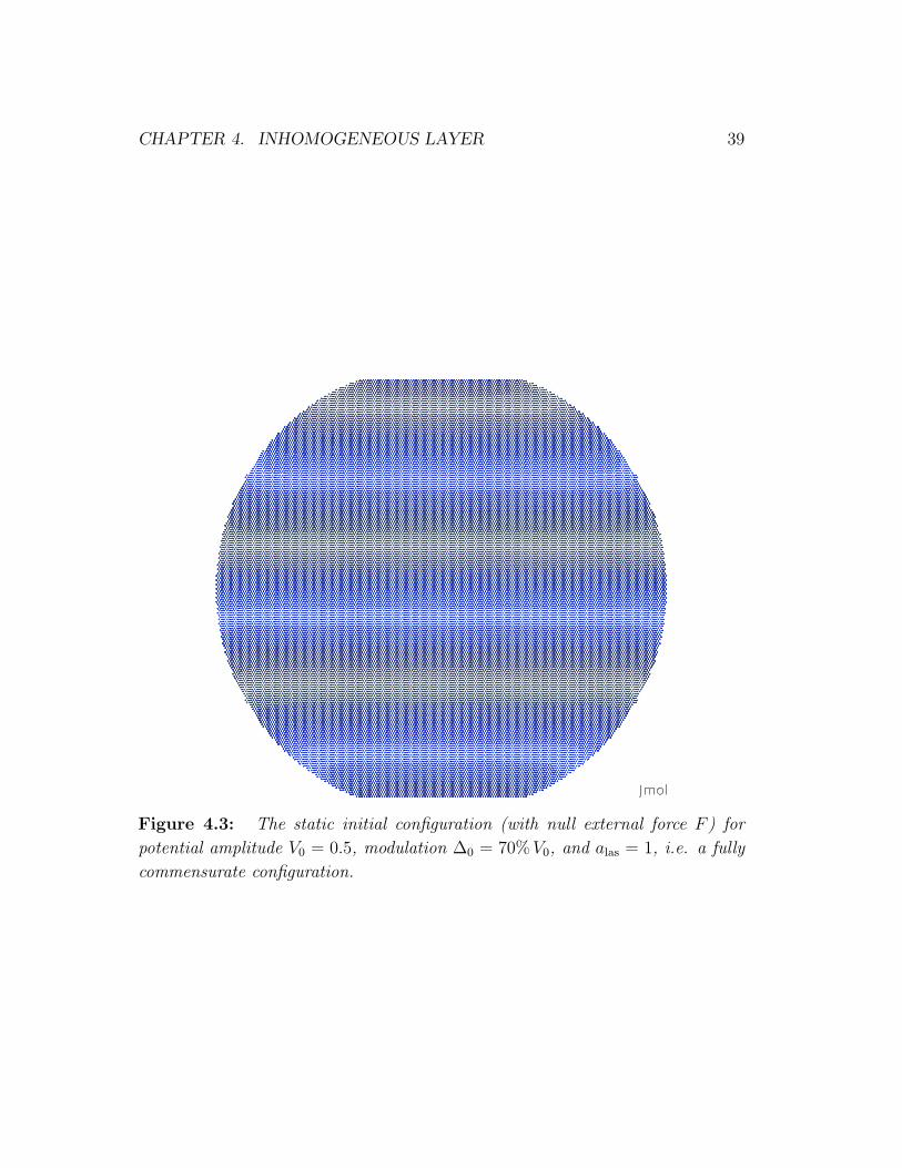
Figure 4.3: The static initial configuration (with null external force F ) for

potential amplitude V0 = 0.5, modulation ∆0 = 70%V0, and alas = 1, i.e. a fully

commensurate configuration.


0 0.5 1 1.5 2F (DC Force)

0

1

2

3

v cm/v

ext

∆0 = 70% V0

Figure 4.4: The Shapiro steps for a fully commensurate configuration (alas =

acoll) obtained with an average external potential of amplitude V0 = 0.5 (in units

defined in Tab. 2.1), oscillation amplitude ∆0 = 70%V0 and oscillation frequency

ν = 0.02, (same parameter used in the incommensurate case of Sec. 3.2.1). The

center-mass velocity is rescaled to the external force as in Fig. 3.2.

and thus undergo little rearrangement. Even with the oscillation modulation

∆0 = 70%V0 no significant relaxation occurs.

Figure 4.3 shows the commensurate colloid configuration after this relax-

ation: we have used a color convention such that darker dots would indicate

colloidal particles sitting at a repulsive point of the corrugation landscape (as in

Fig. 4.5); here we see none, indicating that the structure is relaxed with every

colloid sitting in a potential minimum. Starting from the relaxed configuration,

we run a new simulation with applied external force increased as described above.

Figure 4.4 shows the resulting average center-mass velocity (rescaled with

respect to vext) as a function of the applied external force. We see flat steps at

vcm/vext = 1, 2, 3. This is to be compared with the fixed density result of Fig. 3.6

(red triangles): in the present case the plateau is rounded at the sides, and the

velocity raises continuously from zero to the plateau velocity. Notice also that

the plateau amplitude is reduced, beginning at a force larger and ending at a

smaller force than fixed-density case. The negative-F results obtained during

reciprocation are equivalent, and are then not showed.


Figure 4.5: Initially relaxed configuration for a mismatched configura-

tion (alas/acoll = 14/15) with potential amplitude V0 = 0.5 and modulation

∆0 = 70%V0; light bolder dots mark those particles that belong to regions cor-

responding to repulsive site in the corrugation potential landscape.

4.2 Lattice-mismatched Sistems

In this Section we explore several mismatched configuration, characterized by

different mismatch ratios alas/acoll, and by different values of corrugation V0 and

of the modulation amplitude ∆0.

4.2.1 alas/acoll ≃ 0.93; V0 = 0.5; ∆0 = 70%V0

In a first attempt we investigate Shapiro structures in the same simulation condi-

tions adopted for fixed-density case considered in Sec 3.2, i.e. with the same mis-

match ratio (alas/acoll ≃ 0.93) and with the same potential parameter (V0 = 0.5,

∆0 = 70%V0), but this time in the circular island with the Gaussian confining

potential turned on.

A preliminary relaxation is performed with the protocol already described

for the commensurate OBC case: in Fig. 4.5 we can appreciate the difference

from the corresponding commensurate configuration (Fig. 4.3): here we have a

pattern of bolder particles, that mark those colloids sitting at repulsive points

of the corrugational landscape. The colloids are located along stripes forming


500 1000 1500Time

1.155

1.16

1.165

1.17

Den

sity

Density

0.9925

0.995

0.9975

1

1.0025

a coll

Lattice spacing

Figure 4.6: The time evolution of the colloidal lattice spacing acoll and of

the mean colloid density during relaxation with same parameters as in Fig. 4.5,

but with potential modulation ∆0 = 0. These quantities are obtained as weighted

averages, as discussed in Sec. 4.0.3. The lattice spacing decreases, and the density

increases correspondingly.

1.165

1.17

1.175

1.18

1.185

1.19

Den

sity

Density

1000 2000 3000Time

0.986

0.988

0.99

0.992

0.994

a coll

Lattice spacing

Figure 4.7: Same as Fig. 4.6 but starting from the final configuration of Fig. 4.6

and with the potential modulation ∆0 = 70%V0 turned on. The lattice spacing

further decreases toward commensuration, and correspondingly the density in-

creases.


0.02 0.04 0.06 0.08 0.1F (DC Force)

0.02

0.04

0.06

0.08

0.1

v cm/v ex

t

w

Figure 4.8: The rescaled center of mass velocity (triangles) with same settings

of Fig. 4.7; the w-line (solid line) is computed point by point using Eq. (3.3) and

the local mean lattice spacing: as a result of density fluctuation w is no more a

constant, but decreases as the force increases. With this mismatch ratio and these

potential amplitude parameter no visible plateau is detected.

a pattern of antisoliton lines, intersecting and isolating well-faceted in-registry

regions.

Figure 4.6 reports the variation in time of the mean spacing between col-

loidal particles (and the corresponding density variation) in the region of interest

during the first relaxation: we observe that acoll changes rapidly at the beginning,

to settle at a slightly reduced distance varying later in time. This decrease in

acoll reduces the effective mismatch ratio in the region of interest. When, at the

end of this first simulation, the potential modulation is switched on the mean lat-

tice spacing decreases further (Fig. 4.7), and correspondingly the mean colloidal

density increases, thus taking the system closer to commensuration.

After this relaxation we begin the standard protocol with the application

of an external force in reciprocation. Figure 4.8 reports the rescaled center-

mass velocity as a function of the external force obtained with this setting: no

appreciable subharmonic plateau is detected. As the density changes from one

simulation to the next, we evaluate the value of w corresponding to that density,

i.e. to that mismatch ratio. In Fig. 4.11 the w line tracks the evolution of the

mismatch as a function of the applied force: we find a decreasing function of the

external force F , this behavior reflecting a further decrease in the mean colloidal

spacing alas. To illustrate this evolution Figure 4.9 reports the lattice spacing

as a function of time during two successive computations, one with force F , and


200 400 600 800Time

0.9824

0.9825

0.9826

0.9827

0.9828

a coll

F = 0.03F = -0.03

Figure 4.9: Time evolution of the mean lattice spacing acoll for two successively

applied force values: F = 0.03 and F = −0.03.

one with force −F . At the end, we see that acoll has decreased: acoll ends at a

value smaller than at the starting of both simulations. This systematic decrease

explains the decay of w in Fig. 4.8

4.2.2 alas/acoll = 0.9; V0 = 0.5; ∆0 = 100%V0

To attempt preventing this drift of the system density toward commensuration

firstly we move the mismatch ratio away from unity: we set alas/acoll = 9/10. In

addition we set the modulation amplitude to ∆0 = 100%V0 to widen the step as

in Sec. 3.2.2, thus increasing our chance to detect plateaus.

Figure 4.10 reports the new initial configuration: with this mismatch the an-

tisolitonic pattern is denser, with the antisoliton line mutually closer if compared

to Fig. 4.5. In addition, we changed also the simulation protocol: to improve

the stability of the initial configuration. After the initial relaxation in static con-

dition we run a simulation with a comparably large force F ≃ 1.4, such that

vcm/vext ≃ 2, applied to the particles. We run this simulation for a time t = 200,

significantly shorter than those at smaller forces, to prevent the colloidal parti-

cles to leave the central region of the Gaussian trap. We then apply F = −1.4

as above. After this preliminary forward-backward processing at large force, the

forces are diminished to values F ≃ 0.1 in the region where subharmonic Shapiro

steps are expected, and a further reciprocating relaxation is carried out. After

this preparation the normal protocol for increasing F is followed.

The result is reported in Fig. 4.11: the w-corresponding line is again com-


Figure 4.10: Initial relaxed configuration with a mismatch alas/acoll = 0.9, a

potential value V0 = 0.5 and an amplitude modulation ∆0 = 100%V0. The color

notation is the same as in Fig. 4.5.


0.055 0.06

(b)

0.09

0.1

0.02 0.04 0.06 0.08 0.1F (DC Force)

0.04

0.08

0.12

0.16v cm

/vex

t

(a)

w

Figure 4.11: Same as Fig. 4.8 but with mismatch ratio 0.9 and modulation

amplitude ∆0 = 100%V0. Here a small Shapiro step is detected, as highlighted in

the detail (b). The w line is again computed point by point following the density

variation: now drifts toward commensuration are barely visible.

200 400 600 800Time

0.983

0.984

0.985

0.986

0.987

a coll

alas

= 0.9

F = 0.03

alas

= 0.93

F = 0

F = 0.03

alas

= 0.9

F = 0

Figure 4.12: Comparison between the drift in the mean lattice spacing in going

from F = 0 to F = 0.03 in two different cases: alas = 0.93 (gap highlighted by

the red harrow) and alas = 0.9 (gap highlighted by the dark green harrow); in the

latter case the variation is so small along the whole force range considered that

the resulting w values form a straight line.


0.05 0.1F (DC Force)

0.05

0.1v cm

/vex

t

(a)

0.0875 0.09 0.0925

0.095

0.0975

0.10.1 (b)

w

Figure 4.13: Same as Fig. 4.11 but with V0 = 1. The plateau is again barely

visible, but clearly hinted.

puted point by point as in Fig. 4.8: we see now that the effect of the initial

”dynamical relaxation” is a much more stable density, thus an almost constant

w. A small plateau is now detectable in correspondence of the w-line, better

visible in the inset blowup, Fig. 4.11(b).

4.2.3 alas = 0.9; V0 = 1; ∆0 = 100%V0

As we have seen in Sec. 3.2.2, an increase in the overall corrugation amplitude

causes a increase of the Shapiro steps amplitude: trying to improve the visibility

of the w corresponding plateau we carried out new simulations with a potential

amplitude V0 = 1.

The same protocol as Sec. 4.2.2 is applied: the system is relaxed in absence

of modulation amplitude (∆0 = 0), then with a full oscillating potential (∆0 =

100%V0); finally forward-backward protocol for short (t = 200) times and large

force (F = ±1.4) is applied.

Figure 4.13(a) shows the result obtained under this condition, carrying out

simulation at small forces, starting from the final configuration retrieved at the

end of the discussed preparation protocol: again the w corresponding line is

computed point by point, and a small step, better seen in Fig.4.13(b), in the

rescaled center mass velocity is detectable in correspondence of the computed w

values. As in PBC, also in this non fixed-density case, the potential amplitude

increase causes a decrease in the rescaled vcm: while in Sec. 4.2.2 the step occurs

in a force range 0.055 < F < 0.06, here the step manifests itself in a 0.087 < F <


200 400 600 800Time

0.9866

0.9868

0.987

0.9872

0.9874

a coll

b) F = 0.091F = 0.089

0.9866

0.9868

0.987

0.9872

0.9874

a coll

a) F = 0.061F = 0.058

Figure 4.14: (a) Lattice spacing variation from the beginning (F = 0.058) to

the end (F = 0.061) of the w plateau with V0 = 0.5 . There remain a considerable

density drift during the simulation. (b) same as (a) but with V0 = 1: the drift in

time of the mean colloidal spacing during the simulation at forces corresponding

to the beginning (F = 0.089) and to the end (F = 0.091) of the w plateau is

clearly reduced compared to the the V0 = 0.5 case.


0.091 range to reach the plateau values.

The larger V0 value proves itself beneficial. Indeed a greater stability in the

mean colloid density is observed: while for V0 = 0, Fig. 4.14(a), a drift of the

mean spacing in time is clearly visible, with V0 = 1, the average acoll is remarkably

constant, see Fig. 4.14(b).

Chapter 5

Discussion and Conclusions

The present work addresses, by means of MD simulations, the problem of de-

tecting Shapiro steps structures in a 2D colloidal monolayer interacting with a

periodic corrugation potential that oscillates in space and also in time. In par-

ticular, we attempt to identify the most favorable experimental conditions.

Firstly we investigate this topic in a situation of fixed/controlled colloid

density for both a matched and a mismatched lattice condition: in the former

case only ”trivial” integer steps are present, describing the synchronized peri-

odic advancement of all particles. In mismatched conditions several subharmonic

Shapiro steps are detected: we have investigated closely those structures, trying

to understand the physical mechanism that lies beyond the formation of these

plateaus and trying to characterize those step structures in relation to the partial

motion of solitonic defects crated by the mismatch. In detail we find that the

relation between the velocities of different plateaus reflects the number of col-

loidal particles that advance at each period, the moving particles being generally

a subset of those involved in the formation of the solitonic pattern. We then an-

alyzed how the variation of the corrugation potential parameters (the potential

amplitude V0 and the potential modulation ∆0) influences the step structure: we

find that an increase in V0 involves a shift to higher forces F of the steps and

an increase in their amplitude; on the other hand an increase in ∆0 extends the

steps to smaller F . On the other hand, a very large increasing ∆0 simplifies the

full richness of the subharmonic step structure observed at intermediate ∆0.

We then have moved to more realistic conditions, removing periodic bound-

aries and switching on an overall Gaussian confining potential. A finite circular

cluster trapped in this confining potential realizes a density profile from denser

at the center to slightly more rarefied near its border. Due to the rapidly vary-

ing colloid-colloid repulsion, the density changes are only modest thus realizing

a situation where Shapiro step could be detected. To mitigate the effect of non

50

CHAPTER 5. DISCUSSION AND CONCLUSIONS 51

uniformity, we implemented a smart method to evaluate average values of the

physically significant quantity at play using a smooth function that minimizes

border effects.

Again both lattice matched and mismatched conditions are investigated. In

the matched case, we find again several neat plateaus, but slightly rounded at

their sides: the force range at which these steps occur is nearly the same as in

the fixed-density case.

When we move to mismatched situations we find that the mean density is

varying both in time and as a function of the applied force: increasing F the

average colloid-colloid spacing tend to decrease, slowly approaching full lattice

matching. In an attempt to prevent this drift we increase the mismatch, the

modulation amplitude ∆0 and the potential amplitude. Eventually, thanks also

to a better sample preparation the density as a function of time can be stabi-

lized much better. However, even in the most favorable conditions subharmonic

Shapiro steps are very small and hard to detect.

We conclude that in matched condition the Shapiro step structure can be

easily detected experimentally, with potential amplitude and oscillation modula-

tion values varying in a relative broad ranges. On the other hand in mismatched

condition to detect Shapiro steps experimentally is likely to be a really hard chal-

lenge, also considering thermal and density fluctuation due to defect, which we

ignore in the present simulation. Our prevision is that increasing the potential

amplitude and setting a 100% oscillation amplitude can increase the chances to

reach this goal.

Bibliography

[1] L. Prandtl and Z. Angew, Math. Mech. 8, 85 (1928).

[2] U. Dehlinger: Ann. Phys. (Leipzig) 2, 749 (1929).

[3] O. M. Braun and Y. S. Kivshar, The Frenkel-Kontorova Model: Concepts,

Methods and Applications (Springer-Verlag, Berlin , 2004).

[4] T. Kontorova and Y. Frenkel, Zh. Eksp. Teor. Fiz 8, 1340 (1938).

[5] S. Aubry and P. Y. Le Daeron, Physica D 8, 381 (1983).

[6] M. Peyrard and S. Aubry, J. of Phys. C 16, 1593 (1983).

[7] B. N. J. Persson and E. Tosatti, Physics of Sliding Friction, Springer, Trieste

1996.

[8] A. Socoliuc, E. Gnecco, R. Bennewitz, and E. Meyer Phys. Rev. Lett. 92,

134301 (2004).

[9] E. Ott, Chaos in Dynamical Systems (Cambridge University Press, New York,

2002).

[10] H.Yoshino, T. Nogawa and B. Kim, Prog. Theor. Phys. Supplement 184

(2010).

[11] O. V. Zhirov, G. Casati and D. L. Shepelyansky, Phys. Rev. E 65, 026220

(2002).

[12] B. D. Josephson, Phys. Lett. 1, 251 (1962).

[13] S. Shapiro, Phys. Rev. Lett. 11, 80 (1963); for a review, see: R. L. Kautz,

Rep. Prog. Phys. 59, 935 (1996).

[14] R. P. Feynman, R. Leighton, and M. Sands, The Feynman Lectures on

Physics, The Definitive and Extended Edition (Volume III) (Addison Wes-

ley, New York, 2005).

52

BIBLIOGRAPHY 53

[15] T. Bohlein, J. Mikhael and C. Bechinger, Nature Mater. 11, 126130 (2012).

[16] A. Libal, C. Reichhardt, B. Janko and C. J. Olson Reichhardt, Phys. Rev.

Lett 96, 188301 (2006).

[17] A. Benassi, A. Vanossi, and E. Tosatti, Nature Commun. 2, 236 (2011)

[18] L. M. Floria and J. J. Mazo, Adv. Phys. 45, 505 (1996).

[19] A. Vanossi, N. Manini, M. Urbakh, S. Zapperi, and E. Tosatti, Rev. Mod.

Phys. 85, 529 (2013).

[20] A. Vanossi and E. Tosatti, Nature Mater. 11, 97 (2012).

[21] M. P. Allen and D. J. Tildesley, Computer Simulation of Liquids (Oxford

University Press, New York 1989).

[22] P. T. Korda, G. C. Spalding and D. G. Grier, Phys. Rev. B 66, 024504

(2002).

[23] J. Marchi, Snapping to commensuration: a numerical investigation of the

tendency to epitaxy of lattice mismatched 2D colloidal crystals on peri-

odic optical substrates, Bachelor thesis (Universita d. S. di Milano, 2013).

http://materia.fisica.unimi.it/manini/theses/marchi.pdf.

[24] M. J. Ablowitz, B. Ilan, E. Schonbrun and R. Piestun Phys. Rev. E 74,

035601 (2006).

[25] A. Vanossi, N. Manini and E. Tosatti, Proc. Nati. Acad. Sci. USA 109, 16429

(2012).

[26] A. Vigentini, The Role of Solitons in Sliding Fric-

tion, Bachelor thesis (Universita d. S. di Milano, 2013).

http://materia.fisica.unimi.it/manini/theses/vigentini.pdf.

[27] A. Vigentini, B. Van Hattem, E. Diato, P. Ponzellini, T. Meledina, A.

Vanossi, G. Santoro, E. Tosatti, N. Manini, Phys. Rev. B 89, 094301 (2014).

[28] N. Manini, M. Cesaratto, G. E. Santoro, E. Tosatti, and A. Vanossi, J. Phys.:

Condens. Matter 19, 305016 (2007).

[29] I. E. Castelli, N. Manini, R. Capozza, A. Vanossi, G. E. Santoro, and E.

Tosatti, J. Phys.: Condens. Matter 20, 354005 2008.

[30] I. E. Castelli, R. Capozza, A. Vanossi, G. E. Santoro, N. Manini et al., J.

Chem. Phys. 131, 174711 (2009).

http://materia.fisica.unimi.it/manini/theses/marchi.pdf.

http://materia.fisica.unimi.it/manini/theses/vigentini.pdf.

BIBLIOGRAPHY 54

[31] N. S. Manton and P. M. Sutcliffe, Topological Solitons (Cambridge University

Press, Cambridge 2004).

colloids and pulsing force ﬁelds: eﬀects of spacing mismatch

Documents