Collision resolution

Hash Tables

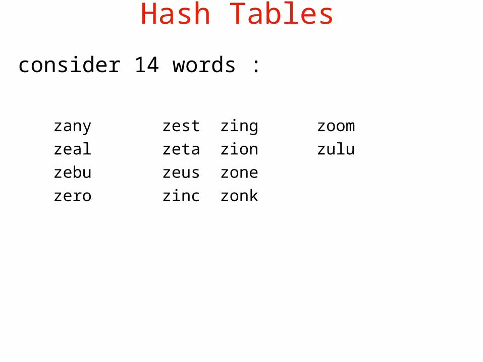
consider 14 words :

zany zest zing zoomzeal zeta zion zuluzebu zeus zone zero zinc zonk

Hash Tables

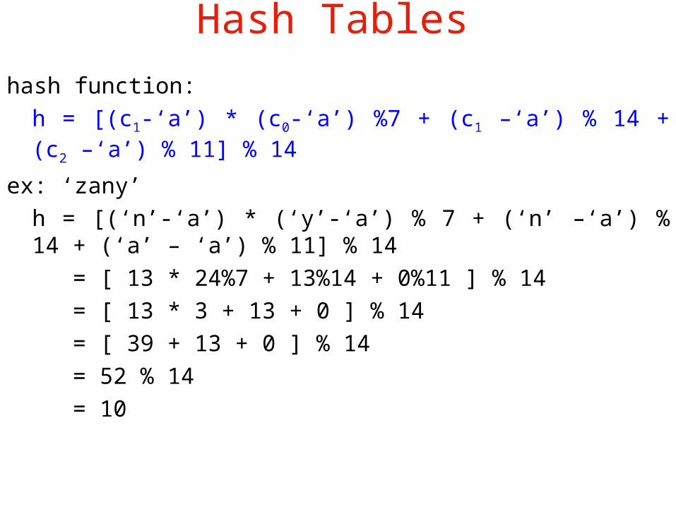
hash function:h = [(c1-‘a’) * (c0-‘a’) %7 + (c1 –‘a’) % 14 + (c2 –‘a’) % 11] % 14

ex: ‘zany’h = [(‘n’-‘a’) * (‘y’-‘a’) % 7 + (‘n’ –‘a’) % 14 + (‘a’ – ‘a’) % 11] % 14 = [ 13 * 24%7 + 13%14 + 0%11 ] % 14 = [ 13 * 3 + 13 + 0 ] % 14 = [ 39 + 13 + 0 ] % 14 = 52 % 14 = 10

Hash Tablesh(“zany ”) = 10h( “zeal” ) = 4h( “zebu” ) = 11h( “zero” ) = 7h( “zest” ) = 0h( “zeta” ) = 9h( “zeus” ) = 6h( “zinc” ) = 5h( “zing” ) = 1h( “zion” ) = 8h( “zone” ) = 12 h( “zonk” ) = 13h( “zoom” ) = 3h( “zulu” ) = 2

minimal perfect hash

The hash function that we used is a special instance of a hash function known as a “minimal perfect hash.”

It is minimal in the sense that the indices it produced are just exactly enough to index the number of actual keys.

It is perfect in the sense that every key is transformed to a unique index value by the hash function. In general, we will not be so fortunate to be able to do this.

Collisions and Resolution:

In our last example our hash table represented an unrealistically fortunate solution.

We achieved O(1) retrieval for all keys as a result of our hash function being a “perfect minimal” hash.

In general, fate will not be quite so co-operative, and when we do find such a hash function, it will most likely become “less than perfect” as soon as we add a new key in our table.

We will now reveal the deep dark truth about the “fourteen four-letter Z-words” that were introduced earlier and the problem that this represents for us.

Hash Tables

Now, for the truth:- there are 15 4-letter z-words!!- the missing word is “zine”- our hash function is no good ... only produces

indices from 0 to 13 ... need 0 to 14 now!- A perfect minimal has may well exist- lets pretend that the best we can do is:

• h(“zine”)=h(“zero”), and one index is left unused.

Collision

When two or more keys collide on the same index, we call this condition a “collision”.

• When a hash function maps two records to the same location we say a “collision” has occurred.

• Obviously two records can’t occupy the same place in the table!

This is a serious problem, and we will have to develop a strategy to deal with it!

Collision resolution

• When a collision occurs, the process of dealing with the collision is known as collision resolution.

• Collision resolution:- involves moving the colliding record to another

location– how? by re-computing the index.

- there are many strategies available for re-computing the index

- each strategy involves “probing” for an empty spot in the table

Collision Resolution with Open Addressing

Linear Probing:

• Linear probing starts with the hash address and searches sequentially for the target key or an empty position.

• Hence this method searches in a straight line, and it is therefore called linear probing.

• The array should be considered circular, so that when the last location is reached, the search proceeds to the first location of the array.

Result of Linear ProbingClustering:• The major drawback of linear probing is that, as the table

becomes about half full, there is a tendency toward clustering; that is, records start to appear in long strings of adjacent positions.

• Thus the sequential searches needed to find an empty position become longer and longer.

Linear Probing leads to sequential Search• Suppose that there are n locations in the array and that the hash

function chooses any of them with equal probability 1/n. Begin with a fairly uniform spread, as shown in the top diagram.

• If a new insertion hashes to location b, then it will go there, but if it hashes to location a (which is full), then it will also go into b. Thus the probability that b will be filled has doubled to 2/n.

• At the next stage, an attempted insertion into any of locations a, b, c,or d will end up in d, so the probability of filling d is 4/n.

• After this, e has probability 5/n of being filled, and so, as additional insertions are made, the most likely effect is to make the string beginning at location a longer and longer.

• Hence the performance of the hash table starts to degenerate toward that of sequential search.

Collision Resolution with Open Addressing

Increment Functions:

• If we are to avoid the problem of clustering, then we must use some more sophisticated way to select the sequence of locations.

• There are many ways to do so. One, called rehashing, uses a second hash function to obtain the second position to consider.

Collision Resolution with Open Addressing

Quadratic Probing:

If there is a collision at hash address h, quadratic probing goes to locations h+1, h+4, h+9, ..., that is, at locations h+i2 (mod hashsize) for i = 1, 2, … .

• Quadratic probing substantially reduces clustering, but it is not obvious that it will probe all locations in the table, and in fact it does not.

• For some values of hash_size the function will probe relatively few positions in the array.

Avoid hash_size as a large power of 2

Quadratic Probing:

• when hash_size is a large power of 2, approximately one sixth of the positions are probed.

• When hash_size is a prime number, however, quadratic probing reaches half the locations in the array.

Collision Resolution with Open Addressing

Other methods:

• Key-dependent increments;• Random probing.

Deletions

• Up to now, we have said nothing about deleting entries from a hash table.

• At first glance, it may appear to be an easy task, requiring only marking the deleted location with the special key indicating that it is empty.

• This method will not work.

Deletions

• The reason is that an empty location is used as the signal to stop the search for a target key. Suppose that, before the deletion, there had been a collision or two and that some entry whose hash address is the now-deleted position is actually stored elsewhere in the table.

• If we now try to retrieve that entry, then the now-empty position will stop the search, and it is impossible to find the entry, even though it is still in the table.

Collision Resolution by Chaining

• Up to now we have implicitly assumed that we are using only contiguous storage while working with hash tables.

• Contiguous storage for the hash table itself is, in fact, the natural choice, since we wish to be able to refer quickly to random positions in the table, and linked storage is not suited to random access.

• There is, however, no reason why linked storage should not be used for the records themselves.

• We can take the hash table itself as an array of linked lists.

Collision Resolution with Chained Hash Tables

Other methods:

• Key-dependent increments;• Random probing.

Collision Resolution with Chained Hash Tables

• The linked lists from the hash table are called chains.

• If the records are large, a chained hash table can save space.

• Collision resolution with chaining is simple; clustering is no problem.

• The hash table itself can be smaller than the number of records; over flow is no problem.

• Deletion is quick and easy in a chained hash table.

• If the records are very small and the table nearly full, chaining may take more space.

Advantages of Chained Hash Tables

• If the records are large, a chained hash table can save space.

• Collision resolution with chaining is simple;

• Clustering is no problem at all, because keys with distinct hash addresses always go to distinct lists.

• The hash table itself can be smaller than the number of records; over flow is no problem.

• Deletion is quick and easy in a chained hash table.

Disadvantage of Chained Hash Tables

• One important disadvantage: All the links require space.

• If the records are large, then this space is negligible in comparison with that needed for the records themselves;

• but if the records are small, then it is not.

Disadvantage of Chained Hash Tables• Suppose, for example, that the links take one word each and that the

entries themselves take only one word (which is the key alone). Such applications are quite common, where we use the hash table only to answer some yes-no question about the key.

• Suppose that we use chaining and make the hash table itself quite small, with the same number n of entries as the number of entries. Then we shall use 3n words of storage altogether: n for the hash table, n for the keys, and n for the links to find the next node (if any) on each chain.

• Since the hash table will be nearly full, there will be many collisions, and some of the chains will have several entries.

• Hence searching will be a bit slow. • Suppose, on the other hand, that we use open addressing. The same 3n

words of storage put entirely into the hash table will mean that it will be only one-third full, and therefore there will be relatively few collisions and the search for any given entry will be faster.

The Birthday Surprise

The Birthday Surprise

• We can determine the probabilities for this question by answering its opposite:

• With m randomly chosen people in a room, what is the probability that no two have the same birthday?

The Birthday Surprise

• Start with any person, and check that person’s birthday off on a calendar.

• The probability that a second person has a different birthday is 364/365. Check it off.

• The probability that a third person has a different birthday is now 363/365.

• Continuing this way, we see that if the first m - 1 people have different birthdays, then the probability that person m has a different birthday is (365 - (m - 1))/365.

The Birthday Surprise

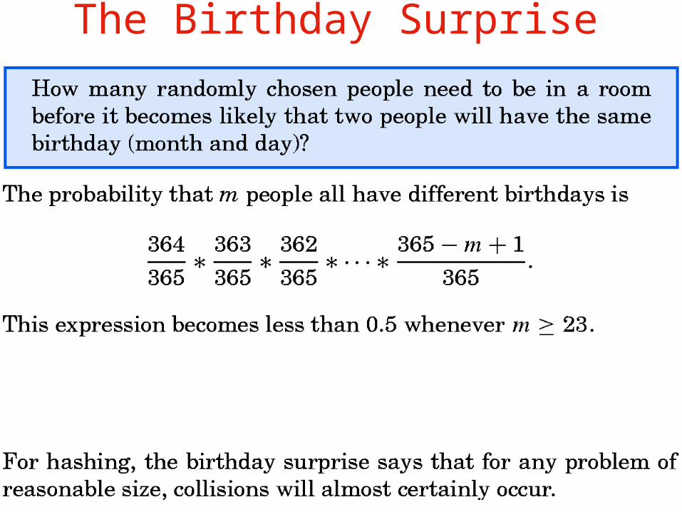
• Since the birthdays of different people are independent, the probabilities multiply (reduces), and we obtain that the probability that m people all have different birthdays is

The Birthday Surprise

• In regard to hashing, the birthday surprise tells us that with any problem of reasonable size, we are almost certain to have some collisions.

• Our approach, therefore, should not be only to try to minimize the number of collisions, but also to handle those that occur as efficiently as possible.

Analysis of Hashing

• As with other methods of information retrieval, we would like to know how many comparisons of keys occur on average during both successful and unsuccessful attempts to locate a given target key.

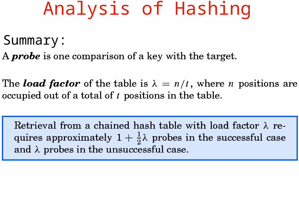
• We shall use the word probe for looking at one entry and comparing its key with the target.

Analysis of Hashing

• The number of probes we need clearly depends on how full the table is.

Analysis of Hashing

• We let n be the number of entries in the table, and we let t (which is the same as hash_size) be the number of positions in the array holding the hash table.

• The load factor of the table is = n/t.

• Thus = 0 signifies an empty table; = 0.5 a table that is half full.

• For open addressing, can never exceed 1, but for chaining there is no limit on the size of .

Analysis of Chaining

• With a chained hash table we go directly to one of the linked lists before doing any probes. Suppose that the chain that will contain the target (if it is present) has k entries. Note that k might be 0.

Analysis of Chaining

• If the search is unsuccessful, then the target will be compared with all k of the corresponding keys. Since the entries are distributed uniformly over all t lists (equal probability of appearing on any list), the expected number of entries on the one being searched is k = = n/t. Hence the average number of probes for an unsuccessful search is .

Analysis of Chaining

• If the search is unsuccessful, then the target will be compared with all k of the corresponding keys. Since the entries are distributed uniformly over all t lists (equal probability of appearing on any list), the expected number of entries on the one being searched is = n/t.

• Hence the average number of probes for an unsuccessful search is .

• As the search will not find an index

Analysis of Chaining

• Now suppose that the search is successful. • From the analysis of sequential search, we know that the average

number of comparisons is ½(k + 1), where k is the length of the chain containing the target.

• But the expected length of this chain is no longer , since we know in advance that it must contain at least one node (the target).

• The n - 1 nodes other than the target are distributed uniformly over all t chains; hence the expected number (k) on the chain with the target is

1 + (n - 1)/t.• Except for tables of trivially small size, we may approximate (n - 1)/t

by n/t = . So, k = 1 + • Hence the average number of probes for a successful search is very

nearly

½(k + 1) = ½(((1+ ) + 1) = 1 + ½

Analysis of Hashing

Summary:

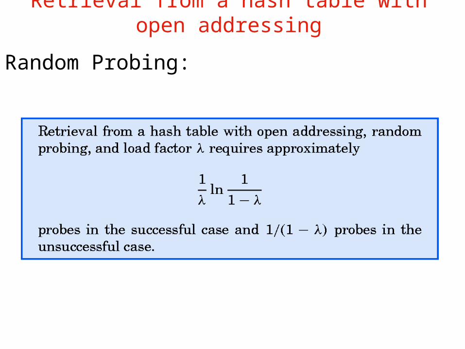
Retrieval from a hash table with open addressing

Random Probing:

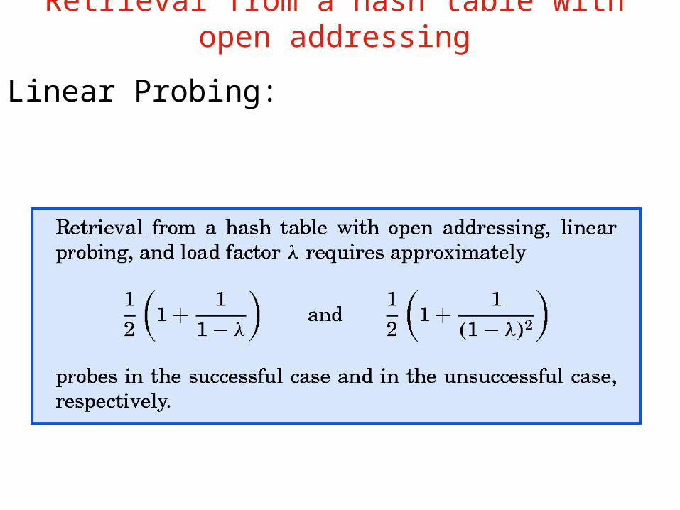
Retrieval from a hash table with open addressing

Linear Probing:

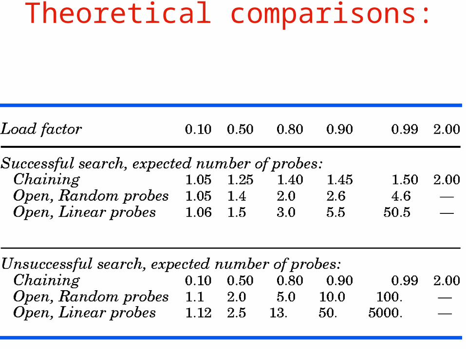
Theoretical comparisons:

Empirical comparisons:

Conclusions: Comparison of MethodsWe have studied four principal methods of information

retrieval, the first two for lists and the second two for tables. Often we can choose either lists or tables for our data structures.

• Sequential search is O(n).

Sequential search is the most flexible method. The data may be stored in any order, with either contiguous or linked representation.

• Binary search is O(log n).

Binary search demands more, but is faster: The keys must be in order, and the data must be in random-access representation (contiguous storage).

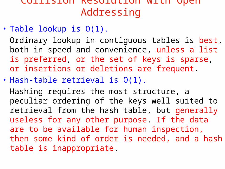
Collision Resolution with Open Addressing

• Table lookup is O(1).Ordinary lookup in contiguous tables is best, both in speed and convenience, unless a list is preferred, or the set of keys is sparse, or insertions or deletions are frequent.

• Hash-table retrieval is O(1).Hashing requires the most structure, a peculiar ordering of the keys well suited to retrieval from the hash table, but generally useless for any other purpose. If the data are to be available for human inspection, then some kind of order is needed, and a hash table is inappropriate.