Collision detection or nearest-neighbor search?On the computational bottleneck insampling-based motion planning?

Michal Kleinbort1??, Oren Salzman2??, and Dan Halperin1

1 Blavatnik School of Computer Science, Tel-Aviv University, Israel2 Carnegie Mellon University, Pittsburgh PA 15213, USA

Abstract. The complexity of nearest-neighbor search dominates theasymptotic running time of many sampling-based motion-planning al-gorithms. However, collision detection is often considered to be the com-putational bottleneck in practice. Examining various asymptotically op-timal planning algorithms, we characterize settings, which we call NN-

sensitive, in which the practical computational role of nearest-neighborsearch is far from being negligible, i.e., the portion of running time takenup by nearest-neighbor search is comparable, or sometimes even greaterthan the portion of time taken up by collision detection. This reinforcesand substantiates the claim that motion-planning algorithms could sig-nificantly benefit from e�cient and possibly specifically-tailored nearest-neighbor data structures. The asymptotic (near) optimality of these al-gorithms relies on a prescribed connection radius, defining a ball arounda configuration q, such that q needs to be connected to all other config-urations in that ball. To facilitate our study, we show how to adapt thisradius to non-Euclidean spaces, which are prevalent in motion planning.This technical result is of independent interest, as it enables to comparethe radial-connection approach with the common alternative, namely,connecting each configuration to its k nearest neighbors (k-NN). Indeed,as we demonstrate, there are scenarios where using the radial connectionscheme, a solution path of a specific cost is produced ten-fold (and more)faster than with k-NN.

1 Introduction

Given a robot R moving in a workspace W cluttered with obstacles, motion-planning (MP) algorithms are used to e�ciently plan a path for R, while avoid-ing collision with obstacles [9, 25]. Prevalent algorithms abstract R as a point in

? This work has been supported in part by the Israel Science Foundation (grantno. 825/15), by the Blavatnik Computer Science Research Fund, and by the HermannMinkowski–Minerva Center for Geometry at Tel Aviv University. O. Salzman hasbeen also supported by the German-Israeli Foundation (grant no. 1150-82.6/2011),by the National Science Foundation IIS (#1409003), Toyota Motor Engineering &Manufacturing (TEMA), and the O�ce of Naval Research. Parts of this work weredone while O. Salzman was a student at Tel Aviv University.

?? M. Kleinbort and O. Salzman contributed equally to this paper.

a high-dimensional space called the configuration space (C-space) X and plan apath (curve) in this space. A point, or a configuration, in X represents a place-ment of R that is either collision-free or not, subdividing X into the sets X

free

and Xforb

, respectively. Sampling-based algorithms study the structure of X byconstructing a graph, called a roadmap, which approximates the connectivityof X

free

. The nodes of the graph are collision-free configurations sampled at ran-dom. Two (nearby) nodes are connected by an edge if the straight line segmentconnecting their configurations is collision-free as well.

Sampling-based MP algorithms are typically implemented using two primi-tive operations: Collision detection (CD) [26], which is primarily used to deter-mine whether a configuration is collision-free or not, and Nearest-neighbor (NN)search, which is used to e�ciently return the nearest neighbor (or neighbors) of agiven configuration. CD is also used to test if the straight line segment connectingtwo configurations lies in X

free

—a procedure referred to as local planning (LP).In this paper we consider both CD and LP calls when measuring the time spenton collision-detection operations.

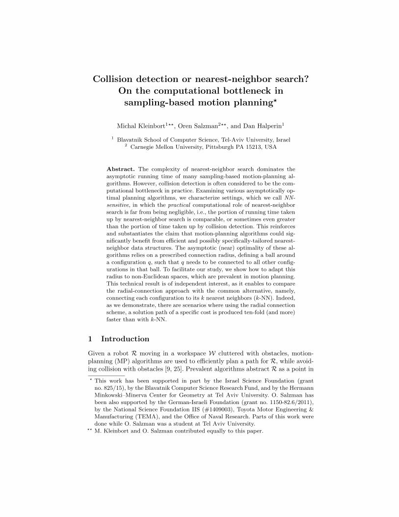
Fig. 1: Running-time breakdown ofthe main primitive operations usedin MPLB [31] applied to the 3D-Grid scenario (Fig. 2a). For additionaldata, see Sec. 4. Best viewed in color.

Contribution The complexity of NN searchdominates the asymptotic running time ofmany sampling-based MP algorithms How-ever, the main computational bottleneck inpractical settings is typically considered to beLP [9, 25]. In this paper we argue that thismay not always be the case. We describe set-tings, which we call NN-sensitive, where the(computational) role of NN search after finiterunning-time is far from negligible and mer-its the use of advanced and specially-tailoreddata structures; see Fig. 1 for a plot demon-strating this behavior. NN-sensitive settings may be due to (i) planners thatalgorithmically shift the computational weight to NN search; (ii) scenarios inwhich certain planners perform mostly NN search; or (iii) parameters’ values forwhich certain planners spend the same order of running time on NN and CD.

Specifically, we focus on asymptotically (near) optimal MP algorithms. Westudy the ratio between the overall time spent on NN search and CD after Nconfigurations were sampled. We observe situations where NN takes up to 100%more time than CD in scenarios based on the Open Motion Planning Library [11];on synthetic high-dimensional C-spaces we even observe a ratio of 4500%.

We mostly concentrate on the radial version of MP algorithms, where theset of neighbors in the roadmap of a given configuration q includes all configu-rations of maximal distance r from q. To do so in non-Euclidean C-spaces, wederive closed-form expressions for the volume of a unit ball in several commonC-spaces. This technical result is of independent interest, as the lack of suchexpressions seems to have thus far prevented the exploration and understand-ing of these types of algorithms in non-Euclidean settings—most experimentalevaluation reported in the literature on the radial version of asymptotically-

2

optimal planners is limited to Euclidean settings only. We show empirically thatin certain scenarios, the radial version of an MP algorithm produces a solutionof specific cost more than ten times faster than the non-radial version, namely,where each node is connected to its k nearest neighbors.

We emphasize that we are not the first to claim that in certain cases NN maydominate the running time of MP algorithms, see, e.g., [5]. However, we take asystematic approach to characterize and analyze when this phenomenon occurs.

Throughout the paper we use the following notation: For an algorithm ALG,let �ALG(S) be the ratio between the overall time spent on NN search and CDfor a specific motion-planning problem after a set S of configurations was sam-pled, where we assume that all other parameters of the problem, the workspaceand the robot, are fixed—see details below. Let �ALG(N) be the expected valueof �ALG(S) over all sample sets S of size N .

Organization We start with an overview of related work in Sec. 2 and continuein Sec. 3 to summarize, for several algorithms, the computational complexityin terms of NN search and CD. We show that asymptotically, as N tends toinfinity, �ALG(N) tends to infinity as well. In Sec. 4 we point out several NN-sensitive settings together with simulations demonstrating how �ALG(N) behavesin such settings. These simulations make use of the closed-form expressions ofthe volume of unit balls, which are detailed in Sec. 5.

2 Background and related work

We start by giving an overview of asymptotically (near) optimal MP algorithmsand continue with a description of CD and NN algorithms.

2.1 Asymptotically optimal sampling-based motion planning

A random geometric graph (RGG) G is a graph whose vertices are sampled atrandom from some space X . Every two configurations are connected if theirdistance is less than a connection radius r

n

(which is typically a function of thenumber of nodes n in the graph). We are interested in a connection radius suchthat, asymptotically, for any two vertices x, y, the cost of a path in the graphconnecting x and y converges to the minimal-cost path connecting them in X .A su�cient condition to ensure this property is that [20]

rn

� 2⌘

✓µ(X

free

)

⇣d

◆1/d

✓1

d

◆1/d

✓log n

n

◆1/d

. (1)

Here d is the dimension of X , µ(·) and ⇣d

denote the Lebesgue measure (volume)of a set and of the d-dimensional unit ball, respectively, and ⌘ � 1 is a tuningparameter that allows to balance between exploring unvisited regions of the C-space and connecting visited regions. Alternatively, an RGG where every vertexis connected to its k

n

� e(1 + 1/d) log n nearest neighbors will ensure similarconvergence properties [21]. Unless stated otherwise, we focus on RGGs of the

3

former type. For a survey on additional models of RGGs, their properties andtheir connection to sampling-based MP algorithms, see [33].

Most asymptotically-optimal planners sample a set of collision-free configu-rations (either incrementally or in batches). This set of configurations inducesan RGG G or a sequence of increasingly dense RGGs {G

n

} whose vertices arethe sampled configurations. Set G0 ✓ G to be the subgraph of G whose edgesrepresent collision-free motions. These algorithms construct a roadmap H ✓ G0.

PRM* and RRG [21] call the local planner for all the edges of G. To increasethe convergence rate to high-quality solutions, algorithms such as RRT* [21],RRT# [1], LBT-RRT [32], FMT* [20], MPLB [31], Lazy-PRM* [14], and BIT* [13]call the local planner for a subset of the edges of G.

Reducing the number of LP calls is typically done by constructing G (usingnearest-neighbor operations only) and deciding for which edges to call the localplanner. Many of the algorithms mentioned do so by using graph operations suchas shortest-path computation. These operations often take a tiny fraction of thetime required for LP computation. However, in more recent algorithms such asFMT* and BIT* this may not be true.

2.2 Collision detection

Most CD algorithms are bound to certain types of models, where rigid polyhe-dral models are the most common. They often allow answering proximity queriesas well (i.e., separation-distance computation or penetration-depth estimation).Several software libraries for collision detection are publicly available [10, 24].The most general of which is the Flexible Collision Library (FCL) [29] that inte-grates several techniques for fast and accurate collision checking and proximitycomputation. For polyhedral models, which are prevalent in MP settings, mostcommonly-used techniques are based on bounding volume hierarchies (BVH).

A collision query using BVHs may take O(m2) time in the worst case,where m is the complexity of the obstacle polyhedra (recall that we assumethat the robot system has constant-description complexity). However, tighterbounds may be obtained using methods tailored for large environments [10, 16].Specifically, the time complexity is O(m log��1 m + s), where � 2 {2, 3} is thedimension of the workspace W and s is the number of intersections between thebounding volumes. Other methods relevant to MP are mentioned in [23]. For asurvey on the topic, see [26].

2.3 Nearest-neighbor methods: exact and approximate

Nearest-neighbor (NN) algorithms are frequently used in various domains. Inthe most basic form of the problem we are given a set P of n points in a metricspace M = (X, ⇢), where X is a set and ⇢ : X⇥X ! R is a distance metric.Given a query point q 2 X, we wish to e�ciently report the nearest point p 2 Pto q. Immediate extensions include the k-nearest-neighbors (K-NN) and the r-near-neighbors (R-NN) problems. The former reports the k nearest points of Pto q, whereas the latter reports all points of P within a distance r from q.

4

In the plane, the NN search problem can be e�ciently solved by constructinga Voronoi diagram of P in O(n log n) time and preprocessing it to a linear-sizepoint-location data structure in O(n log n) time. Queries are then answered inO(log n) time [4, 15]. However, for high-dimensional point sets this approachbecomes infeasible, as it is exponential in the dimension d. This phenomenon isoften termed “the curse of dimensionality” [19].

An e�cient data structure for low dimensional spaces3 is the kd-tree [3, 12],whose expected query complexity is logarithmic in n under certain assumptions.However, the constant factors hidden in the asymptotic query time depend expo-nentially on the dimension d [2]. Another structure suitable for low-dimensionalspaces is the geometric near-neighbor access tree (GNAT); as claimed in [7],typically the construction time is O(dn log n) and only linear space is required.In the extended version [23] we also discuss methods that adapt to the intrinsicdimension of the subspace where the points lie.

All the aforementioned structures give an exact solution to the problem.However, many approximate algorithms exist, and often perform significantlyfaster than the exact ones, especially when d is high. Among the prominentapproximate algorithms are Balanaced box-decomposition trees (BBD-trees) [2],and Locality-sensitive hashing (LSH) [19]. See [18] for a survey on approximateNN methods in high-dimensional spaces.

Finally, we note that in the context of MP, several specifically-tailored ex-act [17, 34] and approximate [22, 30] techniques were previously described. Atheoretical justification for using approximate NN methods rather than exactones is proven in [33] for PRM*.

3 The asymptotic behavior of common MP algorithms

In this section we provide more background on the asymptotic complexity analy-sis of various sampling-based MP algorithms. We then show that for both PRM-type algorithms and RRT-type algorithms, the expected ratio between the timespent on NN search and the time spent on CD goes to infinity as n ! 1.

We denote byN the total number of configurations sampled by the algorithm,and by n the number of collision-free configurations in the roadmap. Let mdenote the complexity of the workspace obstacles and assume that the robot isof constant-description complexity4.

3.1 Complexity of common motion-planning algorithms

We start by summarizing the computational complexity of the primitive oper-ations and continue to detail the computational complexity of a selected set ofalgorithms. We assume familiarity with the planners that are discussed.

3 We refer to a space as low dimensional when its dimension is at most a few dozens.4 The assumption that the robot is of constant-description complexity implies thattesting for self-collision can be done in constant time.

5

Complexity of primitive operations The main primitive operations that weconsider are (i) nearest-neigbhor operations (NN and R-NN) and (ii) collision-detection operations (CD and LP). Additionally, MP algorithms make use ofpriority queues and graph operations. We assume, as is typically the case, thatthe running time of these operations is negligible when compared to NN and CD.

Since many NN data structures require a preprocessing phase, the complexityof a single query should consider the amortized cost of preprocessing. However,since usually at least n NN or R-NN queries are performed, where n is thenumber of points stored in the NN data structure, this amortized preprocessingcost is asymptotically subsumed by the cost of a query.

A list of the common complexity bounds for the di↵erent types of NN queriescan be found in the extended version of this paper [23]. As mentioned in Sec. 2.2,the complexity of a single CD operation for a robot of a constant-description com-plexity can be bounded by O(m log��1 m+ s), where � 2 {2, 3} is the dimensionof the workspace and s is the number of intersections between the boundingvolumes, which is O(m2) in the worst case. On the other hand, for a systemwith ` such robots, a CD operation is composed of ` single robot CD queriesas well as O(`2) robot-robot collision checks. Local planning (LP) is often im-plemented using multiple CD operations along a densely-sampled C-space line-segment between two configurations. Specifically, we assume that the planneris endowed with a fixed parameter called STEP specifying the sampling den-sity along edges. During LP, edges of maximal length r

n

will be subdivided intodr

n

/STEPe collision-checked configurations (see also [25, p. 214]). Therefore, thecomplexity of a single LP query can be bounded by O(r

n

· QCD), where QCD isthe complexity of a single CD query (here STEP is assumed to be constant).

Complexity of algorithms In order to choose which edges of G to explicitlycheck for being free, all algorithms need to determine (i) which of theN nodes arecollision free and (ii) what are the neighbors of each node. Thus, these algorithmstypically require N CD calls and n R-NN calls.

To quantify the number of LP calls performed by each algorithm, note thatthe expected number of neighbors of a node in G is ⇥(⌘d2d log n) [33]. Therefore,if an algorithm calls the local planner for all (or for a constant fraction of) theedges of G, then the expected number of LP calls will be ⇥(⌘d2dn log n).

3.2 The asymptotic behavior of the ratio �ALG(N)

Let TCD(S) be the overall time spent on CD for a specific motion-planningproblem after a set S of configurations was sampled, where we assume, as before,that all other parameters of the problem are fixed. Let TCD(N) be the expectedvalue of TCD(S) over all sample sets S of size N . We show here that the expectedvalue �ALG(N) of the ratio over all sample sets of sizeN goes to infinty asN ! 1for both sPRM* and RRT*. Recall that we are interested in the expected valueof the ratio. We do that by looking at the ratio between a lower bound on thetime of NN and TCD(N), defined above.

To obtain a lower bound on the time of NN, we assume that the NN structurebeing used is a j-ary tree for a constant j, in which the data points are kept

6

in the leaves. This is a reasonable assumption, as many standard NN structuresare based on trees [2, 3, 7, 12]. Performing n queries of NN (or R-NN) usingthis structure, one for every data point, costs ⌦(n log n), as each query involveslocating the leaf in which the query point lies. It is easy to show this both forsPRM*, in which the NN structure is constructed given a batch of all data points,and for RRT*, where the structure is constructed incrementally.

Additionally, we have the following lemma, whose proof is in [23]:

Lemma 1 If an algorithm uses a uniform set of samples and the C-space ob-stacles occupy a constant fraction of the C-space, then n = ⇥(N) almost surely.

For sPRM* it holds that TCD(N) = #CD ·QCD+#LP ·QLP. Clearly, #CD = Nand QCD = O(m2) (see Sec. 3.1). In expectation we have that #LP = O(n2 · rd

n

)

and in addition QLP = O(rn

·QCD). Finally, recall that rn = ⇥⇣2⌘ (log n/n)1/d

⌘=

⇥�(log n/n)1/d

�. Therefore,

TCD(N) = N ·QCD +O(⌘d2dn log n) ·QLP

= N ·QCD +O(⌘d2dn log n) ·O(rn

·QCD)

= O(m2N) +O(m2N1�1/d log1+1/d N) = O(m2N). (2)

As ⌦(n log n) is a valid lower bound on the overall complexity of NN, thereexists a constant c

2

> 0 s.t. the time for NN for a roadmap with n nodes is atleast c

2

n log n. Moreover, since TCD(N) = O(m2N) then there exists a constantc3

> 0 s.t. the overall time for CD is at most c3

m2N .Thus, using Lemma 1, �sPRM*(N) � c2n logn

c3m2N

� c

0logN

m

2 , where c0 > 0 is aconstant. Observing that the above fraction goes to infinity as N goes to infinity,we obtain that lim

N!1 �sPRM*(N) = 1, as anticipated.We note that althoughm is assumed to be constant, we leave it in our analysis

to emphasize its e↵ect on �ALG(N). In summary,

Proposition 2 The values �sPRM*(N) and �RRT*(N) tend to infinity as N ! 1.

The proof for �RRT*(N) can be found in the extended version [23].From a theoretical standpoint, NN search determines the asymptotic running

time of typical sampling-based MP algorithms. In contrast, the common expe-rience is that CD dominates the running time in practice. However, we show inthe remainder of the paper that in a variety of special situations NN search is anon-negligible factor in the running-time in practice.

4 Nearest-neighbor sensitive settings

In this section we describe settings where the computational role of NN searchin practice is far from negligible, even for a relatively small number of samples.We call these settings NN-sensitive. For each such setting we empirically demon-strate this behavior. In Sec. 4.1 we describe our experimental methodology andoutline properties common to all our experiments. Each of the subsequent sec-tions is devoted to a specific type of NN-sensitivity.

7

(a) (b) (c) (d)

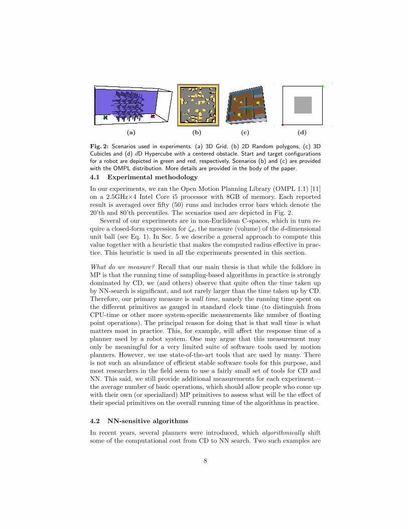
Fig. 2: Scenarios used in experiments. (a) 3D Grid, (b) 2D Random polygons, (c) 3DCubicles and (d) dD Hypercube with a centered obstacle. Start and target configurationsfor a robot are depicted in green and red, respectively. Scenarios (b) and (c) are providedwith the OMPL distribution. More details are provided in the body of the paper.

4.1 Experimental methodology

In our experiments, we ran the Open Motion Planning Library (OMPL 1.1) [11]on a 2.5GHz⇥4 Intel Core i5 processor with 8GB of memory. Each reportedresult is averaged over fifty (50) runs and includes error bars which denote the20’th and 80’th percentiles. The scenarios used are depicted in Fig. 2.

Several of our experiments are in non-Euclidean C-spaces, which in turn re-quire a closed-form expression for ⇣

d

, the measure (volume) of the d-dimensionalunit ball (see Eq. 1). In Sec. 5 we describe a general approach to compute thisvalue together with a heuristic that makes the computed radius e↵ective in prac-tice. This heuristic is used in all the experiments presented in this section.

What do we measure? Recall that our main thesis is that while the folklore inMP is that the running time of sampling-based algorithms in practice is stronglydominated by CD, we (and others) observe that quite often the time taken upby NN-search is significant, and not rarely larger than the time taken up by CD.Therefore, our primary measure is wall time, namely the running time spent onthe di↵erent primitives as gauged in standard clock time (to distinguish fromCPU-time or other more system-specific measurements like number of floatingpoint operations). The principal reason for doing that is that wall time is whatmatters most in practice. This, for example, will a↵ect the response time of aplanner used by a robot system. One may argue that this measurement mayonly be meaningful for a very limited suite of software tools used by motionplanners. However, we use state-of-the-art tools that are used by many. Thereis not such an abundance of e�cient stable software tools for this purpose, andmost researchers in the field seem to use a fairly small set of tools for CD andNN. This said, we still provide additional measurements for each experiment—the average number of basic operations, which should allow people who come upwith their own (or specialized) MP primitives to assess what will be the e↵ect oftheir special primitives on the overall running time of the algorithms in practice.

4.2 NN-sensitive algorithms

In recent years, several planners were introduced, which algorithmically shiftsome of the computational cost from CD to NN search. Two such examples are

8

Lazy-PRM* [14] and MPLB [31], though lazy planners were described before(e.g., [6]). Both algorithms delay local planning by building an RGG G over aset of samples without checking if the edges are collision free. Then, they employgraph-search algorithms to find a solution. To construct G only NN queries arerequired. Moreover, using these graph-search algorithms dramatically reducesthe number of LP calls. Thus, in many cases (especially as the number of samplesgrows) the weight of CD is almost negligible with respect to that of NN.

Specifically, Lazy-PRM* iteratively computes the shortest path in G betweenthe start and target configurations. LP is called only for the edges of the path. Ifsome are found to be in collision, they are removed from the graph. This processis repeated until a solution is found or until the source and target do not lie inthe same connected component. We use a batch variant of Hauser’s Lazy-PRM*algorithm [14], which we denote by Lazy-sPRM*. This variant constructs theroadmap in the same fashion as sPRM* does but delays LP to the query phase.

MPLB uses G to compute lower bounds on the cost between configurationsto tightly estimate the cost-to-go [31]. These bounds are then used as a heuris-tic to guide the search of an anytime version of FMT* [20]. The bounds arecomputed by running a shortest-path algorithm over G from the target to thesource. Fig. 1 (on page 2) presents the amount of NN, CD and other operationsused by MPLB running on the 3D Grid scenario for two robots translating androtating in space that need to exchange their positions (Fig. 2a). With severalthousands of iterations, which are required for obtaining a high-quality solution,NN dominates the running time of the algorithm. For additional details see [23].

Additional experiments demonstrating the behavior of NN-sensitive algo-rithms can be found in [5, 14, 31].

4.3 NN-sensitive scenarios

A scenario S = (W,R) is defined by a workspace W and a robot system R. Therobot system R may, in turn, be a set of ` single constant-description complexityrobots operating simultaneously inW. Let the dimension d of S be the dimensionof the C-space induced by R, and, hence, d = ⇥(`). Let the complexity of S bethe complexity m of the workspace obstacles. Note that CD is a↵ected by `, asboth robot-obstacle and robot-robot collisions should be considered. Therefore,the bound on the complexity of a CD operation is: O(` ·m2 + `2), see Sec. 3.1.

We next show how the role of NN may increase when (i) the dimension of Sincreases or (ii) the complexity of S decreases.

The e↵ect of the dimension d Proposition 2 states that as the number ofsamples tends to infinity, NN dominates the running time of the algorithm. Anatural question to ask is “what happens when we fix the number of samples andincrease the dimension?” The di↵erent structure of RRT* and sPRM* merits adi↵erent answer for each algorithm.

RRT* Here, we show that the NN sensitivity grows with the number of un-successful iterations5. This implies that if the number of unsuccessful iterations

5 Here, an iteration is said to be unsuccessful when the RRT* tree is not extended.

9

0.0

0.5

1.0

1.5

2.0RRT*(N)

15 20 25 30 35Dimension

N = 80KN = 40KN = 20K

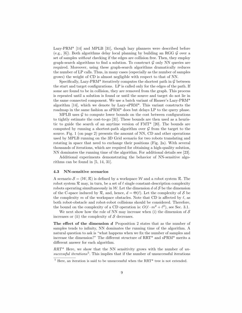
Fig. 3: �RRT*(N) as a function of d inthe 3D Cubicles scenario (Fig. 2c), whenfixing the number N of iterations.

d #NN #R-NN #CD #LP-A #LP-B #CD in LP

12 80K 10.2K 80K 80K 325K 4,235K

24 80K 7.5K 80K 80K 724K 4,135K

36 80K 5.7K 80K 80K 886K 3,812K

Table 1: Average number of calls for the mainprimitive operations for di↵erent values of d, forN = 80K iterations.

grows with the dimension, so will �RRT*(N). Indeed, we demonstrate this phe-nomenon in the 3D cubicles scenario (Fig. 2c). Note that in this situation thee↵ect of d is indirect.

To better discuss our results we define two types of LP operations: the first iscalled when the algorithm attempts to grow the tree towards a random samplewhile the second is called during the rewiring step. We denote the former typeof LP calls by LP-A and the latter by LP-B and note that LP-A will occur everyiteration while LP-B will occur only in successful ones.

We use ` translating and rotating L-shaped robots. We gradually increase `from two to six, resulting in a C-space of dimension d = 6`. Robots are placed indi↵erent sections of the workspace and can reach their target with little robot-robot interaction. We fix N and measure �RRT*(N) as a function of d. The resultsfor several values of N are depicted in Fig. 3. Additionally, Table 1 shows theaverage number of operation calls for various values of d.

As d grows, the number of unsuccessful iterations grows (see #LP-A in Ta-ble 1). This growth, which is roughly linear with respect to d induces a linearincrease in �RRT*(N) for a given N (see Fig. 3). Furthermore, the slope of thisline increases with N which further demonstrates the fact that for a fixed d,lim

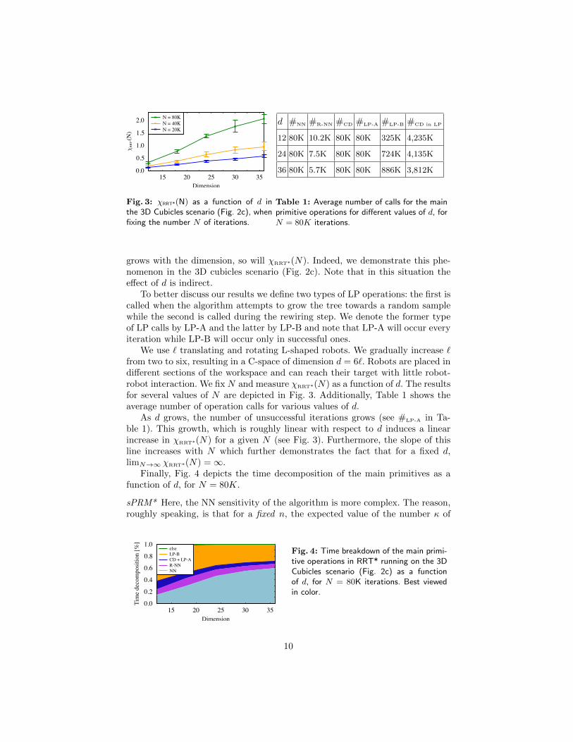
N!1 �RRT*(N) = 1.Finally, Fig. 4 depicts the time decomposition of the main primitives as a

function of d, for N = 80K.

sPRM* Here, the NN sensitivity of the algorithm is more complex. The reason,roughly speaking, is that for a fixed n, the expected value of the number of

0.0

0.2

0.4

0.6

0.8

1.0

Timedecomposition[%]

15 20 25 30 35Dimension

elseLP-BCD + LP-AR-NNNN

Fig. 4: Time breakdown of the main primi-tive operations in RRT* running on the 3DCubicles scenario (Fig. 2c) as a functionof d, for N = 80K iterations. Best viewedin color.

10

0.0

0.5

1.0

1.5

2.0

2.5sPRM

*(N)

5 10 15 20 25 30 35 40 45 50Dimension

rNN, = 0.5rNN, = 0.25rNN, = 0

(a)

0

9

18

27

36

45

sPRM

*(N)

5 10 15 20 25 30 35 40 45 50Dimension

kNN, = 0.5kNN, = 0.25kNN, = 0

(b)

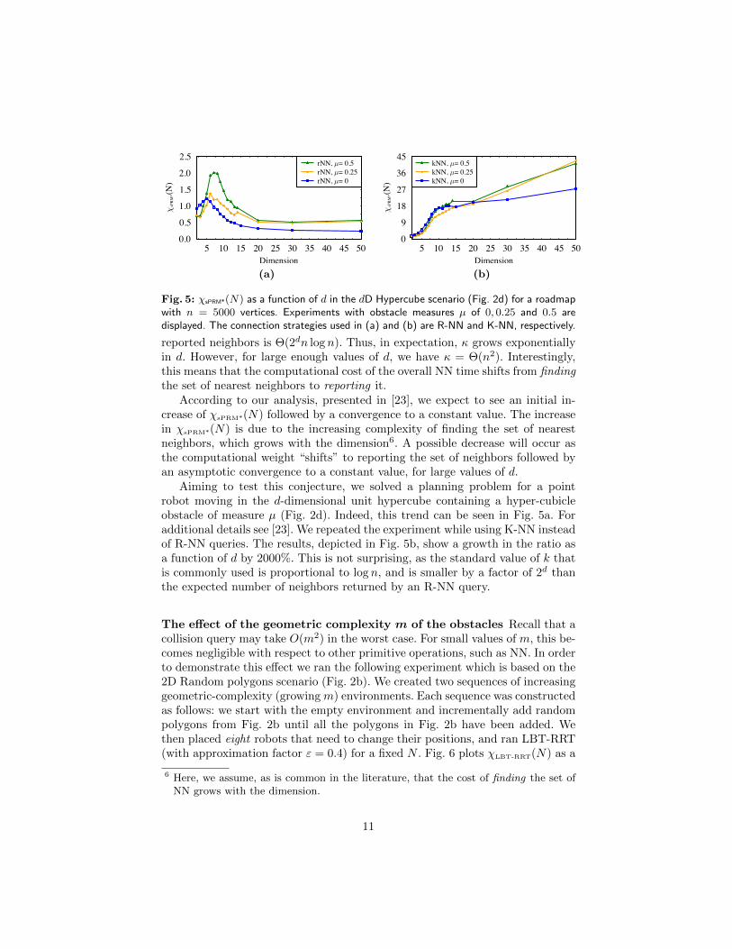
Fig. 5: �sPRM*(N) as a function of d in the dD Hypercube scenario (Fig. 2d) for a roadmapwith n = 5000 vertices. Experiments with obstacle measures µ of 0, 0.25 and 0.5 aredisplayed. The connection strategies used in (a) and (b) are R-NN and K-NN, respectively.

reported neighbors is ⇥(2dn log n). Thus, in expectation, grows exponentiallyin d. However, for large enough values of d, we have = ⇥(n2). Interestingly,this means that the computational cost of the overall NN time shifts from findingthe set of nearest neighbors to reporting it.

According to our analysis, presented in [23], we expect to see an initial in-crease of �sPRM*(N) followed by a convergence to a constant value. The increasein �sPRM*(N) is due to the increasing complexity of finding the set of nearestneighbors, which grows with the dimension6. A possible decrease will occur asthe computational weight “shifts” to reporting the set of neighbors followed byan asymptotic convergence to a constant value, for large values of d.

Aiming to test this conjecture, we solved a planning problem for a pointrobot moving in the d-dimensional unit hypercube containing a hyper-cubicleobstacle of measure µ (Fig. 2d). Indeed, this trend can be seen in Fig. 5a. Foradditional details see [23]. We repeated the experiment while using K-NN insteadof R-NN queries. The results, depicted in Fig. 5b, show a growth in the ratio asa function of d by 2000%. This is not surprising, as the standard value of k thatis commonly used is proportional to log n, and is smaller by a factor of 2d thanthe expected number of neighbors returned by an R-NN query.

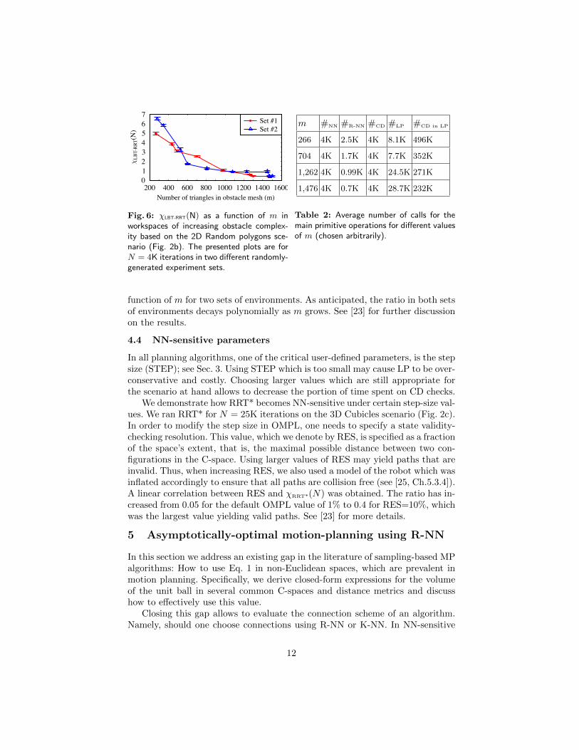
The e↵ect of the geometric complexity m of the obstacles Recall that acollision query may take O(m2) in the worst case. For small values of m, this be-comes negligible with respect to other primitive operations, such as NN. In orderto demonstrate this e↵ect we ran the following experiment which is based on the2D Random polygons scenario (Fig. 2b). We created two sequences of increasinggeometric-complexity (growingm) environments. Each sequence was constructedas follows: we start with the empty environment and incrementally add randompolygons from Fig. 2b until all the polygons in Fig. 2b have been added. Wethen placed eight robots that need to change their positions, and ran LBT-RRT(with approximation factor " = 0.4) for a fixed N . Fig. 6 plots �LBT-RRT(N) as a

6 Here, we assume, as is common in the literature, that the cost of finding the set ofNN grows with the dimension.

11

01234567

LBT-RRT(N)

200 400 600 800 1000 1200 1400 1600Number of triangles in obstacle mesh (m)

Set #1Set #2

Fig. 6: �LBT-RRT(N) as a function of m inworkspaces of increasing obstacle complex-ity based on the 2D Random polygons sce-nario (Fig. 2b). The presented plots are forN = 4K iterations in two di↵erent randomly-generated experiment sets.

m #NN #R-NN #CD #LP #CD in LP

266 4K 2.5K 4K 8.1K 496K

704 4K 1.7K 4K 7.7K 352K

1,262 4K 0.99K 4K 24.5K 271K

1,476 4K 0.7K 4K 28.7K 232K

Table 2: Average number of calls for themain primitive operations for di↵erent valuesof m (chosen arbitrarily).

function of m for two sets of environments. As anticipated, the ratio in both setsof environments decays polynomially as m grows. See [23] for further discussionon the results.

4.4 NN-sensitive parameters

In all planning algorithms, one of the critical user-defined parameters, is the stepsize (STEP); see Sec. 3. Using STEP which is too small may cause LP to be over-conservative and costly. Choosing larger values which are still appropriate forthe scenario at hand allows to decrease the portion of time spent on CD checks.

We demonstrate how RRT* becomes NN-sensitive under certain step-size val-ues. We ran RRT* for N = 25K iterations on the 3D Cubicles scenario (Fig. 2c).In order to modify the step size in OMPL, one needs to specify a state validity-checking resolution. This value, which we denote by RES, is specified as a fractionof the space’s extent, that is, the maximal possible distance between two con-figurations in the C-space. Using larger values of RES may yield paths that areinvalid. Thus, when increasing RES, we also used a model of the robot which wasinflated accordingly to ensure that all paths are collision free (see [25, Ch.5.3.4]).A linear correlation between RES and �RRT*(N) was obtained. The ratio has in-creased from 0.05 for the default OMPL value of 1% to 0.4 for RES=10%, whichwas the largest value yielding valid paths. See [23] for more details.

5 Asymptotically-optimal motion-planning using R-NN

In this section we address an existing gap in the literature of sampling-based MPalgorithms: How to use Eq. 1 in non-Euclidean spaces, which are prevalent inmotion planning. Specifically, we derive closed-form expressions for the volumeof the unit ball in several common C-spaces and distance metrics and discusshow to e↵ectively use this value.

Closing this gap allows to evaluate the connection scheme of an algorithm.Namely, should one choose connections using R-NN or K-NN. In NN-sensitive

12

settings this choice may have a dramatic e↵ect on the performance of the algo-rithm since (i) the number of reported neighbors may di↵er and (ii) the cost ofthe two query types for a certain NN data structure may be di↵erent. Indeed,we show empirically that there are scenarios where using R-NN, a solution pathof a specific cost is produced ten-fold (and more) faster than with K-NN.

Due to lack of space, some of the technical details and experiments appearonly in the extended version of this paper [23].

5.1 Well-behaved spaces and the volume of balls

Recall that X denotes a C-space and that given a set A ✓ X , µ(A) denotes theLebesgue measure of A. Let ⇢ : X ⇥ X ! R denote a distance metric and letB⇢

X (r, x) := {y 2 X|⇢(x, y) r} and S⇢

X (r, x) := {y 2 X|⇢(x, y) = r} denotethe ball and sphere of radius r (defined using ⇢) centered at x 2 X , respectively.Finally, let B⇢

X (r) := µ (B⇢

X (r, 0)) and S⇢X (r) := µ (S⇢

X (r, 0)). We will often omitthe superscript ⇢ or the subscript X when they will be clear from the context.

We now define the notion of a well-behaved space in the context of metrics;for a detailed discussion on well-behaved spaces see [27]. In such spaces there isa derivative relationship between S(r) and B(r). Formally,

Definition 3 A space X is well behaved when @BX (r)

@r

= SX (r). Conversely, wesay that X is well behaved when

R%2[0,r]

SX (%)d% = BX (r).

We continue with the definition of a compound space which is the Cartesianproduct of two spaces. Let X

1

,X2

be two C-spaces with distance metrics ⇢1

, ⇢2

,respectively. Define X = X

1

⇥ X2

to be their compound space. We adopt acommon way to define the (weighted) distance metric over X , when using weights

w1

, w2

2 R+ and some constant p [25, Chapter 5]: ⇢X = (w1

⇢p1

+ w2

⇢p2

)1/p

.7

The following Lemma states that the volume of balls in a compound spaceX = X

1

⇥ X2

where X1

is well behaved can be expressed analytically.

Lemma 4 Following the above notation, if X1

is well behaved then

BX1⇥X2(r) =

Z

%2[0,r/w

1/p1 ]

SX1(%) · BX2

✓rp � w

1

%p

w2

◆1/p

!d%. (3)

Proof. By definition, BX (r) =Rx2BX (r)

dx. Using Fubini’s Theorem [28],

BX1⇥X2(r) =

Z

x12BX1 (r/w1/p1 )

0

B@Z

x22BX2

✓r

p�w1x

p

1w2

◆1/p! dx

2

1

CA dx1

.

The inner integral is simply the volume of a ball of radius⇣

r

p�w1xp

1w2

⌘1/p

in X2

.

In addition, we know that X1

is well behaved, thus BX1(r) =Rx12BX1 (r)

dx =

7 This distance metric is often used due to its computational e�ciency and simplic-ity. However, alternative methods exist, which exhibit favorable properties such asinvariance to rotation of the reference frame; see, e.g., [8].

13

X

x

r

nB(rn

, x)

(a)

1.01.11.21.31.41.5

Solutioncost

0 10 20 30 40 50 60 70 80Time [sec]

K-NNR-NN Heuristic

(b)

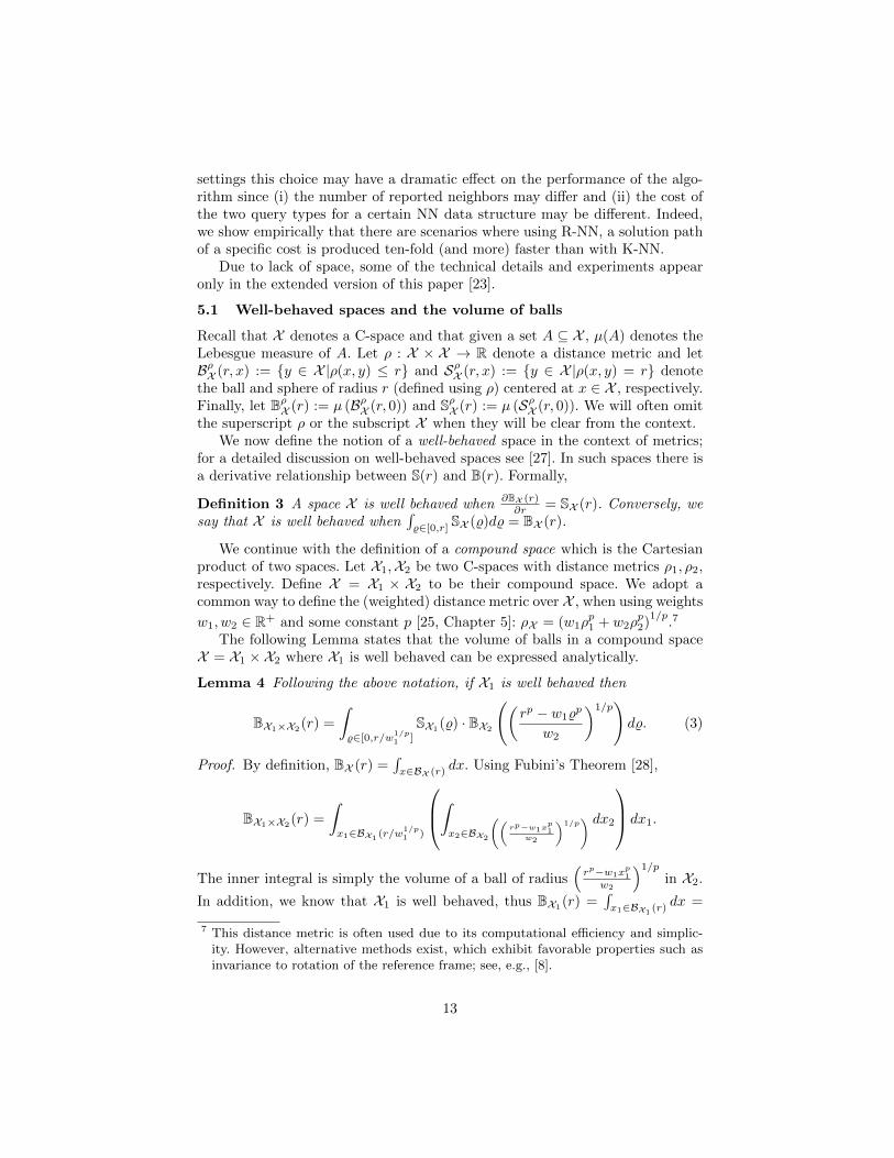
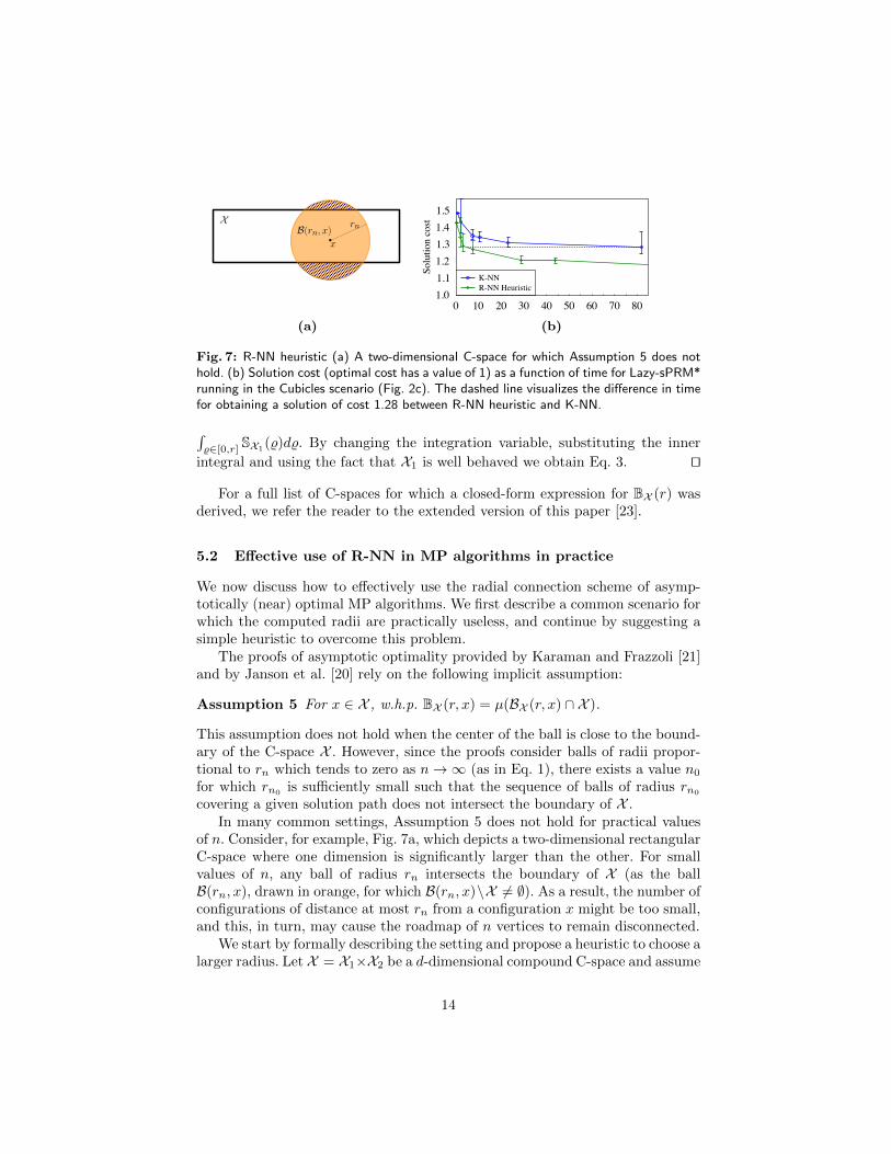
Fig. 7: R-NN heuristic (a) A two-dimensional C-space for which Assumption 5 does nothold. (b) Solution cost (optimal cost has a value of 1) as a function of time for Lazy-sPRM*running in the Cubicles scenario (Fig. 2c). The dashed line visualizes the di↵erence in timefor obtaining a solution of cost 1.28 between R-NN heuristic and K-NN.

R%2[0,r]

SX1(%)d%. By changing the integration variable, substituting the innerintegral and using the fact that X

1

is well behaved we obtain Eq. 3. ut

For a full list of C-spaces for which a closed-form expression for BX (r) wasderived, we refer the reader to the extended version of this paper [23].

5.2 E↵ective use of R-NN in MP algorithms in practice

We now discuss how to e↵ectively use the radial connection scheme of asymp-totically (near) optimal MP algorithms. We first describe a common scenario forwhich the computed radii are practically useless, and continue by suggesting asimple heuristic to overcome this problem.

The proofs of asymptotic optimality provided by Karaman and Frazzoli [21]and by Janson et al. [20] rely on the following implicit assumption:

Assumption 5 For x 2 X , w.h.p. BX (r, x) = µ(BX (r, x) \ X ).

This assumption does not hold when the center of the ball is close to the bound-ary of the C-space X . However, since the proofs consider balls of radii propor-tional to r

n

which tends to zero as n ! 1 (as in Eq. 1), there exists a value n0

for which rn0 is su�ciently small such that the sequence of balls of radius r

n0

covering a given solution path does not intersect the boundary of X .In many common settings, Assumption 5 does not hold for practical values

of n. Consider, for example, Fig. 7a, which depicts a two-dimensional rectangularC-space where one dimension is significantly larger than the other. For smallvalues of n, any ball of radius r

n

intersects the boundary of X (as the ballB(r

n

, x), drawn in orange, for which B(rn

, x)\X 6= ;). As a result, the number ofconfigurations of distance at most r

n

from a configuration x might be too small,and this, in turn, may cause the roadmap of n vertices to remain disconnected.

We start by formally describing the setting and propose a heuristic to choose alarger radius. Let X = X

1

⇥X2

be a d-dimensional compound C-space and assume

14

that µ(X1

) � µ(X2

). Let d1

, d2

denote the dimensions of X1

,X2

, respectively.Finally, let ⇢

max(X2)be the maximal distance between any two points in X

2

andassume that ⇢ = w

1

⇢1

+ w2

⇢2

. When Assumption 5 does not hold, as in Fig. 7,the intuition is that the “e↵ective dimension” of our C-space is closer to d

1

thanto d

1

+ d2

. If rn

> w2

⇢max(X2)

then 8x 2 X BX (rn

, x) > µ(BX (rn

, x) \ X ). Insuch cases, we suggest to project all points to X

1

and use the critical connectionradius that we would have used had the planning occurred in X

1

.To evaluate the proposed heuristic, we ran Lazy-sPRM* on the Cubicles

scenario (Fig. 2c) using R-NN with and without the heuristic, and also using K-NN strategy (with the standard k

n

value). We measured the cost of the solutionpath as a function of the running time. As depicted in Fig. 7b, the heuristicwas able to find higher-quality solutions using less samples, resulting in a ten-fold speedup in obtaining a solution of a certain cost, when compared to K-NN.Moreover, R-NN without the heuristic was practically inferior, as it was not ableto find a solution even for large values of n; results omitted.

References

[1] Arslan, O., Tsiotras, P.: Use of relaxation methods in sampling-based algorithmsfor optimal motion planning. In: ICRA. pp. 2413–2420 (2013)

[2] Arya, S., Mount, D.M., Netanyahu, N.S., Silverman, R., Wu, A.Y.: An optimalalgorithm for approximate nearest neighbor searching in fixed dimensions. Journalof the ACM 45(6), 891–923 (1998)

[3] Bentley, J.L.: Multidimensional binary search trees used for associative searching.Commun. ACM 18, 509–517 (1975)

[4] de Berg, M., Cheong, O., van Kreveld, M., Overmars, M.: Computational Geom-etry: Algorithms and Applications. Springer-Verlag, 3rd edn. (2008)

[5] Bialkowski, J., Otte, M.W., Karaman, S., Frazzoli, E.: E�cient collision checkingin sampling-based motion planning via safety certificates. I. J. Robotic Res. 35(7),767–796 (2016)

[6] Bohlin, R., Kavraki, L.E.: Path planning using lazy PRM. In: ICRA. pp. 521–528(2000)

[7] Brin, S.: Near neighbor search in large metric spaces. In: VLDB. pp. 574–584(1995)

[8] Chirikjian, G.S., Zhou, S.: Metrics on motion and deformation of solid models. J.Mech. Des. 120(2), 252–261 (1998)

[9] Choset, H., Lynch, K.M., Hutchinson, S., Kantor, G., Burgard, W., Kavraki, L.E.,Thrun, S.: Principles of Robot Motion: Theory, Algorithms, and Implementation.MIT Press (June 2005)

[10] Cohen, J.D., Lin, M.C., Manocha, D., Ponamgi, M.: I-COLLIDE: an interactiveand exact collision detection system for large-scale environments. In: Symposiumon Interactive 3D Graphics. pp. 189–196, 218 (1995)

[11] Sucan, I.A., Moll, M., Kavraki, L.E.: The Open Motion Planning Library. IEEERobotics & Automation Magazine 19(4), 72–82 (2012)

[12] Friedman, J.H., Bentley, J.L., Finkel, R.A.: An algorithm for finding best matchesin logarithmic expected time. ACM Trans. Math. Softw. 3(3), 209–226 (1977)

[13] Gammell, J.D., Srinivasa, S.S., Barfoot, T.D.: Informed RRT*: Optimal sampling-based path planning focused via direct sampling of an admissible ellipsoidal heuris-tic. In: IROS. pp. 2997–3004 (2014)

15

[14] Hauser, K.: Lazy collision checking in asymptotically-optimal motion planning.In: ICRA. pp. 2951–2957 (2015)

[15] Hemmer, M., Kleinbort, M., Halperin, D.: Optimal randomized incremental con-struction for guaranteed logarithmic planar point location. Comput. Geom. 58,110–123 (2016)

[16] Hubbard, P.M.: Approximating polyhedra with spheres for time-critical collisiondetection. ACM Trans. Graph. 15(3), 179–210 (1996)

[17] Ichnowski, J., Alterovitz, R.: Fast nearest neighbor search in SE(3) for sampling-based motion planning. In: WAFR. pp. 197–214 (2014)

[18] Indyk, P.: Nearest neighbors in high-dimensional spaces. In: Goodman, J.E.,O’Rourke, J. (eds.) Handbook of Discrete and Computational Geometry, chap. 39,pp. 877–892. CRC Press LLC, Boca Raton, FL, 2nd edn. (2004)

[19] Indyk, P., Motwani, R.: Approximate nearest neighbors: Towards removing thecurse of dimensionality. In: STOC. pp. 604–613 (1998)

[20] Janson, L., Schmerling, E., Clark, A.A., Pavone, M.: Fast marching tree: A fastmarching sampling-based method for optimal motion planning in many dimen-sions. I. J. Robotic Res. 34(7), 883–921 (2015)

[21] Karaman, S., Frazzoli, E.: Sampling-based algorithms for optimal motion plan-ning. I. J. Robotic Res. 30(7), 846–894 (2011)

[22] Kleinbort, M., Salzman, O., Halperin, D.: E�cient high-quality motion planningby fast all-pairs r-nearest-neighbors. In: ICRA. pp. 2985–2990 (2015)

[23] Kleinbort, M., Salzman, O., Halperin, D.: Collision detection or nearest-neighborsearch? On the computational bottleneck in sampling-based motion planning.CoRR abs/1607.04800 (2016)

[24] Larsen, E., Gottschalk, S., Lin, M.C., Manocha, D.: Fast proximity queries withswept sphere volumes. Tech. rep., Department of Computer Science, Universityof North Carolina (1999), TR99-018

[25] LaValle, S.M.: Planning Algorithms. Cambridge University Press (2006)[26] Lin, M.C., Manocha, D.: Collision and proximity queries. In: Goodman, J.E.,

O’Rourke, J. (eds.) Handbook of Discrete and Computational Geometry, chap. 35,pp. 767–786. CRC Press LLC, Boca Raton, FL, 2nd edn. (2004)

[27] Marichal, J.L., Dor↵, M.: Derivative relationships between volume and surfacearea of compact regions in Rd. Rocky Mountain J. Math. 37(2), 551–571 (2007)

[28] Mazzola, G., Milmeister, G., Weissmann, J.: Comprehensive Mathematics forComputer Scientists 2, chap. 31, pp. 87–95. Springer, Berlin, Heidelberg (2005)

[29] Pan, J., Chitta, S., Manocha, D.: FCL: A general purpose library for collision andproximity queries. In: ICRA. pp. 3859–3866 (2012)

[30] Plaku, E., Kavraki, L.E.: Quantitative analysis of nearest-neighbors search inhigh-dimensional sampling-based motion planning. In: WAFR. pp. 3–18 (2006)

[31] Salzman, O., Halperin, D.: Asymptotically-optimal motion planning using lowerbounds on cost. In: ICRA. pp. 4167–4172 (2015)

[32] Salzman, O., Halperin, D.: Asymptotically near-optimal RRT for fast, high-quality, motion planning. IEEE Trans. Robotics 32(3), 473–483 (2016)

[33] Solovey, K., Salzman, O., Halperin, D.: New perspective on sampling-based motionplanning via random geometric graphs. Robots Science and Systems (RSS) (2016)

[34] Yershova, A., LaValle, S.M.: Improving motion-planning algorithms by e�cientnearest-neighbor searching. IEEE Trans. Robotics 23(1), 151–157 (2007)

16