University of Anbar – College of Engineering

Departement of Civil Engineering

Highway Materials

Course No:CE 4345

Prepared By:

Dr Talal H. Fadhil

Dr Taher M. Ahmed

B. Aggregates:

B.1. General, Crushed aggregates, Natural aggregate, Slags, Demolition

materials, Artificial aggregates, Recycled (pulverised) aggregates,.

B.2. Geometrical properties determination:

Aggregate sizes, Particle size distribution – sieving method, Aggregate size,

Sieving procedure, and gradation curve determination.

B.3. Basic aggregate tests:

Resistance to fragmentation by the Los Angeles test, Resistance to impact test,

Particle density and water absorption tests, Determination of density of coarse

aggregate particles by wire-basket method, Determination of density of fine

aggregate particles, Determination of density of aggregate particles less than

0.063 by pycnometer method, Magnesium sulfate test, Flat particles, elongated

particles or flat and elongated particles test, Crushed and broken surfaces test,

and Sand equivalent test.

B.4. Blending two or more aggregates:

Trial-and-error method, Mathematical methods, and Graphical method.

B. Aggregates:

B.1. General

There are two main uses of aggregates in civil engineering: as an underlying

material for foundations and pavements and as ingredients in portland cement

and asphalt concretes.

• Aggregate underlying materials, or base courses, can add stability to a

structure, provide a drainage layer, and protect the structure from frost

damage. Stability is a function of the interparticle friction between the

aggregates and the amount of clay and silt ―binder‖ material in the voids

between the aggregate particles. However, increasing the clay and silt content

will block the drainage paths between the aggregate particles.

• In portland cement concrete, 60% to 75% of the volume and 79% to 85% of

the weight is made up of aggregates. The fine aggregate particles act as a

filler to reduce the amount of cement paste needed in the mix.

• In asphalt concrete, aggregates constitute over 80% of the volume and 92% to

96% of the mass. The asphalt cement acts as a binder to hold the aggregates

together.

2. Aggregate Sources

• Natural sources for aggregates include gravel pits, river run deposits, and

rock quarries. Crushed stones are the result of processing rocks from

quarries. Usually, gravel deposits must also be crushed to obtain the needed

size distribution, shape, and texture.

• Manufactured aggregates can use slag waste from steel mills and

expanded shale and clays to produce lightweight aggregates.

Geologists classify rocks into three basic types: igneous, sedimentary,

and metamorphic.

1. Igneous rocks are primarily crystalline and are formed by the cooling of

molten rock magma as it moves toward or on the surface of the earth. It is

classified based on grain size and composition. Coarse grains and fine

grains. Based on composition is a function of the silica content, specific

gravity and color.

2. Sedimentary rocks are primarily formed either by the deposition of insoluble

residue from the disintegration of existing rocks or from deposition of the

inorganic remains of marine animals. Classification is based on the predominant

mineral present as calcareous (limeston, chalks, etc.), siliceous (chert,

sandstone, etc), or argillaceous (shale, etc).

3. Metamorphic rocks form from igneous or sedimentary rocks that are drawn

back into the earth‘s crust and exposed to heat and pressure, re-forming the

grain structure. Metamorphic rocks generally have a crystalline structure, with

grain sizes ranging from fine to coarse

• SLAGS: Slags are by-products that are produced during the production

process of metals such as iron and nickel.

• DEMOLITION MATERIALS: Demolition materials are used in subbase or

base layers after preselection and crushing.

• ARTIFICIAL AGGREGATES: Artificial aggregates are mainly produced from

the calcination of rocks such as bauxite. Calcined bauxite has good antiskid

properties. Other types of aggregates are designated by their low density or

specific gravity (unit weight) and are used mainly in producing lightweight

concrete.

• Pulverised pavement materials are also known as recycled asphalt pavement

(RAP). They are produced by crushed and screening old asphalt materials

during reconstruction projects. They can be used as an aggregate replacement

in new asphalt materials. It is widely used all over the world at the moment in

highway construction.

B.2. Geometrical Properties Determination

Aggregate Sizes

Aggregates are divided into coarse aggregates, fine aggregates and fillers.

• Fine aggregate are defined as aggregates whose particles pass through a

4.75 mm sieve (No. 4) and retained on a 0.075 mm sieve (No. 200).

• Coarse aggregates are defined as aggregates whose particles are retained

on 4.75 mm sieve (No. 4).

• Fillers are most of which pass through 0.075 mm sieve (No. 200). It is

added to construction materials to provide certain properties.

RECYCLED (PULVERISED) AGGREGATES:

Particle Size Distribution – Sieving Method

•Gradation describes the particle size distribution of the aggregate

which is found by sieving analysis. The particle size distribution is

an important property of the aggregates. The surface area of

coarse aggregates is lesser than fine aggregate so the binder

requiered for coarse aggreagte is less than that for fine

aggreagtes. Hence, construction considerations, such as

dimensions of construction members, clearance between

reinforcing steel, and layer thickness, limit the maximum

aggregate size.

•Two definitions are used to describe the maximum aggregate

size:

1.Maximum aggregate size—the smallest sieve size through

which 100% of the aggregates sample particles pass.

2.Nominal maximum aggregate size—the largest sieve that

retains any of the aggregate particles, but generally not more than

10%.

• Gradation is evaluated by passing the aggregates through a

series of sieves, as shown in Figure.

• Gradation results are described by the cumulative percentage

of aggregates that either pass through or are retained by a

specific sieve size. Then, gradation analysis results are

generally plotted on a semilog chart.

• The density of an aggregate mix is a function of the size

distribution of the aggregates. The relationship for determining

the distribution of aggregates that provides the dense graded

or maximum density (minimum amount of voids) is:

Dense Graded Gradation

Where: Pi is passing a sieve of size di, D = maximum size of the aggregate.

The value of the exponent n recommended by Fuller is 0.5. In the 1960s, the

Federal Highway Administration (FHWA) recommended a value of 0.45 for n

and introduced the ―0.45 power‖ gradation chart

• A dense-graded is a well-graded gradation aggregate

Example:

The data in the table below represents set of sieves. Plot the sieve distribution

curve by using Fuller and FHWA equations.

Other Types of Gradation

In addition to the dense graded (well-graded) aggregates, There are other

characteristic distributions, as shown in Figure.

• A uniform graded is a one-sized distribution, it has the majority of aggregates

passing one sieve and being retained on the next smaller sieve. Hence, the

majority of the aggregates have essentially the same diameter; their gradation

curve is nearly vertical. One-sized graded aggregates will have good

permeability, but poor stability, and are used in such applications as chip seals

of pavements.

• Open-graded aggregates are missing

small aggregate sizes (fine) that would

block the voids between the larger

aggregate. Since there are a lot of voids,

the material will be highly permeable,

but may not have good stability.

• Gap-graded aggregates are missing

one or more sizes of material

(intermediat sizes) . Their gradation

curve has a near horizontal section

indicating that nearly the same portions

of the aggregates pass two different

sieve sizes.

Particle Shape and Surface Texture

B.3. Basic aggregate tests:

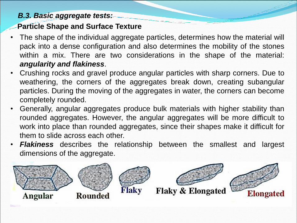
• The shape of the individual aggregate particles, determines how the material will

pack into a dense configuration and also determines the mobility of the stones

within a mix. There are two considerations in the shape of the material:

angularity and flakiness.

• Crushing rocks and gravel produce angular particles with sharp corners. Due to

weathering, the corners of the aggregates break down, creating subangular

particles. During the moving of the aggregates in water, the corners can become

completely rounded.

• Generally, angular aggregates produce bulk materials with higher stability than

rounded aggregates. However, the angular aggregates will be more difficult to

work into place than rounded aggregates, since their shapes make it difficult for

them to slide across each other.

• Flakiness describes the relationship between the smallest and largest

dimensions of the aggregate.

• The roughness of the aggregate surface plays an important role in the way the

aggregate compacts and bonds with the binder material. Aggregates with a

rough texture are more difficult to compact into a dense configuration than

smooth aggregates. Rough texture generally improves bonding and increases

interparticle friction. In general, natural gravel and sand have a smooth texture,

whereas crushed aggregates have a rough texture.

• For the purpose of preparing portland cement concrete, it is desirable to use

rounded and smooth aggregate particles to improve the workability of fresh

concrete during mixing. However, angular and rough particles are desirable for

asphalt concrete and base courses in order to increase the stability of the

materials in the field and to reduce rutting.

• Flaky and elongated aggregates are undesirable for asphalt concrete, since

they are difficult to compact during construction and are easy to break.

• A crushed particle exhibits one or more mechanically induced fractured faces

and typically has a rough surface texture.

• To evaluate the angularity and surface texture of coarse aggregate, the

percentages of particles with one and with two or more crushed faces are

counted in a representative sample.

• According to ISSRB for surface and binder courses, the degree of crushing at

least is 90% by weight of the materials retained on sieve No. 4 has one of more

fractuerd faces. And less tha 10% for flat and elongated pieces with more than

5 to 1 between maximum and minimum dimension.

Resistance to fragmentation by the Los Angeles test: (AASHTO T – 96)

The ability of aggregates to resist to the effect of loads is related to the hardness

of the aggregate particles and is described as the toughness or abrasion

resistance. The aggregate must resist crushing and degradation when placed,

compacted, and exposed to loads.

The mass of tested aggregate sample is 5000 ± 5 g (W1). In this test, aggregates

sample is placed in a large steel drum (diameter 70 cm and hieght 50 cm) rotated

typically for 500 revolutions (30 – 33 RPM); 11 iron balls, diameter 4.8 cm and

weight of each is 445 gm, are put inside the drum with the aggregate.

After completion of the test, the aggregates are sieved on sieve No. 12 (1.7 mm)

and the mass of the passed material is (W2).

The lower the Los Angeles value, the more durable and resistant the aggregate to

fragmentation.

Note: according to ISSRB, percent of wear (LAV) for aggregate coarser than

2.36 mm (No. 8) is not more than 30% for surfac course and 35% for binder

course and 40% for base course.

Resistance to impact test:

The resistance impact test is an alternative test to the resistance to

fragmentation by the Los Angeles test, a relative measure of the resistance of

an aggregate to sudden shock or impact. A sample of a dried aggregate passing

sive size 12.5 mm and retaind on sieve 10 mm is taken and is put into a metal

mould (diameter 10 mm) with three layers, each layer is compacted by steel rod

(d= 10 mm, l= 230 mm) 25 blows.

The wieght of this sample is taken

(W1) and then pourd into another steel

container of the impact machien. The

sample is exposed to 15 blows droped

from a height of 370 mm. After

crushing, the aggregate is sieved

through sieve 2.36 mm (No. 8) and

than weighed (W2). The impact

crushing value (ICV) is:

Soundness and Durability

The ability of aggregate to withstand weathering is defined

as soundness or durability. Aggregates used in various civil

engineering applications must be sound and durable,

particularly if the structure is subjected to severe climatic

conditions. Water freezing in the voids of aggregates

generates stresses that can fracture the stones. The

soundness test (ASTM C88) simulates weathering by

soaking the aggregates in either a sodium sulfate or a

magnesium sulfate solution. These sulfates cause crystals

to grow in the aggregates, simulating the effect of freezing.

The test starts with an oven-dry sample separated into

different sized fractions. The sample is subjected to 5

cycles of soaking in the sulfate for (16 to 18) hours at 21±1 oC followed by drying. Afterwards, the aggregates are

washed by water with barium chloride (BaCl2) (at 43 ± 6°C)

through the samples in their containers and dried, each

size is weighed, and the weighted average percentage loss

for the entire sample is computed.

According to ISSRB the loss due to soundness test for coarse aggreagte is

less than 12% when sodium sulfate is used and less tha 18% for magnesium

sulfate is used.

Sand Equivalent Test

This test is conducted to determine quickly the relative proportion of the clay-like

materials in fine aggregate and granular soils. A low sand equivalent value

indicates the presence of clay proportion. This is detrimental to the quality of the

aggregate and characterises the aggregates as ‗non-clean‘.

From a representative sample, a mass of 120 g of

dried material is placed into a graduated transparent

cylinder. A portion of calcium chloride solution is added

to the cylinder until it reaches about 100 mm. The

contents of the cylinder are left undisturbed for about

10 min and then, after loosening the material from the

bottom and placing a stopper, it is shaken manually

(more than 90 times) or in a mechanical shaker for 30

± 1 s. Then, more calcium chloride solution is added to

the cylinder until the cylinder is filled to the 380 ± 0.25

mm graduation mark. The cylinder and its content are

then left undisturbed for 20 min. During this period, the

material settles out from suspension to form two

distinctive layers. The height of the clay suspension

(hc) and the height of the sand reading (hs) are taken.

The sand equivalent (SE) is calculated by the

following formula:

Particle Density and Water Absorption tests:

Aggregates can capture water and asphalt binder in surface voids. The amount of

absorbed water by aggregates is important in the design of Portland Cement

Concrete (PCC) and for Hot Mix Asphalt (HMA). Aggregate‘s absorption must be

evaluated to determine the appropriate amount of water for PCC mix design. Also,

absorption is important for asphalt concrete, where, highly absorptive aggregates

require greater amounts of asphalt binder, making the HMA more expensive.

• For coarse aggregate, the AASHTO method

(AASHTO T85) requires the sample be immersed for a

period of 15–19 h while the ASTM method (ASTM

C127) specifies an immersed period of 24 ± 4 h. After

the specimen is removed from the water, it is rolled in

an absorbent towel until all visible films of water are

removed. This is defined as the saturated surface dry

(SSD) condition. Three mass measurements are

obtained from a sample: (i) the SSD mass, (ii) water

submerged mass, and (iii) the oven dry mass from

which the value of Gsb (bulk specific gravity of

stone (aggregate)) of an aggregate can be

determined.

Specific Gravity of Coarse Aggregate:

Coarse Aggregate Specific Gravity (ASTM C127, AASHTO T 85)

Dry then saturate the aggregates

Dry to SSD condition and weigh

Measure submerged weight

Measure dry weight

(1)

(2)

(3)

(4)

(5)

• For fine aggregate, both methods: AASHTO T84 and ASTM C128 are

similar, except for the required period in which a sample of fine

aggregate is submersed in water to essentially fill the pores. The

AASHTO procedure requires immersion of fine aggregate in water

for 15–19 h, while the ASTM method specifies a soaking period of

24 ± 4 h. In both methods, the soaked sample is then spread on a pan

and exposed to a gentle current of warm air until approaching to

saturated surface dry condition. The aggregate is lightly tamped into a

cone-shaped (4cm top diameter, 9 cm bottom diameter, and 7 cm

height) mold with 25 light drops of the tamper (340± 15g). If the tamped

fine aggregate keep the same shape of the cone when the mold is

removed, the fine aggregate is assumed to have excess moisture, and it

needs to further drying. When the cone of sand just begins to slump

upon removal of the mold, it is assumed to have reached the SSD

condition. Three masses are determined from the method using either

gravimetric or volumetric methods; (i) SSD, (ii) saturated sample in

water, and (iii) oven dry which are used to calculate Gsb.

Specific Gravity of Fine Aggregate:

Fine Aggregate Specific Gravity (ASTM C128 & AASHTO T 84)

Pycno-meter used for FA

Specific Gravity

To find saturated surface dry of FA

Filler’ Tests:

Mineral filler : Mineral filler shall consists of limestone or other stone

dust. Portland cement, hydrated lime or other inert non-plastic mineral

matter from approved sources.

Mineral fillers shall be thoroughly dried and free from lumps of

aggregations of fine particles. It shall confirm to the grading requirements

as shown in table below.

The plasticity index (PI) as determined by AASHTO T90 shall not be

greater than 4.

Specific Gravity of Fillers:

Depending on the react of filler with water, there are two types which are used in

HMA production, react and non-react with water. For example, limestone dust is

non-react with water while cement is react, so the procedure for determining the

specific gravity (sp.gr) for the filler is as shown below:

• Specific gravity of the filler is the ratio of the mass of a given volume of the filler

to that of an equal volume of water at the same condition of temperature.

•The specific gravity of Portland cement is generally about (3.12-3.19). Cement

will react with water, so to prevent this reaction kerosene should be used instead

of water to be mixed with cement.

Testing procedure

1. Weight mass of the empty pycnometer with stopper = m1.

2. Fill the pycnometer with measuring liquid. Replace stopper carefully, allowing

excess liquid to escape through the hole in the stopper. Make sure there are

no bubbles. Dry outside and weight = m4.

3. Fill the dry, empty pycnometer about 1/3 full of the sample. Closed it and

weight again = m2.

4. Add measuring liquid to the sample. Fill pycnometer about 2/3 full. Mix up with

caution and refill with the liquid, closed the pycnometer and weight = m3.

5. Calculate the mass of the sample from formula: m = m2 - m1.

6. Count the density from the basic formula.

where m is mass of the sample of the tested material (m = m2 – m1)

m1 mass of dry empty pycnometer including stopper

m2 mass of dry pycnometer with sample and stopper

m3 mass of closed pycnometer with sample and measuring liquid

m4 mass of the closed pycnometer with measuring liquid including stopper.

m5 mass of the closed pycnometer with water including stopper.

ρk density of measuring liquid at tested temperature

Note: Measuring liquid could not be water in case of measuring cement

density usually is used kerosene or any liquid non-react with cement.

,

B.4. Blending Two or More Aggregates:

Introduction

The blending of aggregates is a process in which two, three, or more of

aggregates, which have different types of sources and sizes, are mixed together

to give a blend with a specified gradation.

The blending of aggregates is done because:

1- There are no individual sources, sizes, and types of aggregates (natural or

artificial) that individually can supply aggregate of gradation to meet a specific

or desired gradation.

2- It is more economical to use some natural sands or rounded aggregates in

addition to crushed or manufactured aggregates, and this process (mixing

natural and crushed) cannot be held without using a blending operation.

Regardless of which method will be used, there are two important pieces of

information that must be known before finding the proportion values. These are

the sieve analysis of each material, and the limits of desired specifications.

Trial-and-error method

Trial-and-error method: Is the most common method of determining the proportions

of aggregate which meets specification requirements. The designer, who has high

of experience, can estimate the percentage value of each aggregate contributes in

the blend. He also can predict the first approximation value by interpreting the

sieve analysis of each type and desired gradation. By repeating the trial process

several times, the contribution of each one can be estimated.

Mathematical Methods

Mathematical method: depending on the basic formula of this method which is true

for any number of aggregates combined.

𝑃 = 𝐴·𝑎 + 𝐵·𝑏 + 𝐶·𝑐 +⋯ ⋯ ⋯ ⋯ ⋯ ⋯ ⋯ ⋯ ⋯ ⋯ ⋯(1)

a + b + c + ⋯ = 1 ⋯ ⋯ ⋯ ⋯ ⋯ ⋯ ⋯ ⋯ ⋯ ⋯(2)

Where

P is the percentage of material passing through a given sieve for the combined

aggregates A, B, C which represents the mid point of the specification for a given

sieve.

A, B, and C are the percentages of material passing a given sieve for aggregates

A, B, C, respectively.

a, b, and c are the proportions of aggregate A, B, and C used in the combination.

For blending two types of aggregate A and B:

𝑃 = 𝐴·𝑎 + 𝐵·𝑏, 𝑎 + 𝑏 = 1.

For blending three types of aggregate A, B and C:

The following data listed in the table below, the following notes can be drawn

As shown from the table, the majority of contribution for aggregate greater than

sieve No. 8 is coming from aggregate (A) because the amount of aggregate

passing of sieve (No. 8) are 82 % and 100 % for aggregates B and C respectively

while from A the % passing is 3.2 (it means that the amount of retaining on sieve

NO. 8 are 96.8, 18 and 0 for A, B and C respectively).

Applying Equation (4) to find the contribution of aggregate A (a)

The percentage of sieve No. 200 are to be examined, by applying Equation (1).

Now applying Equation (2).

b + c = 1 - 0.5 = 0.5 b = 0.5 – c (ii)

Substituting Equation (ii) in (i) yields:

c = 0.03 b = 0.5 - 0.03= 0.47

7 = 0 × 0.5 + 9.2×𝑏 + 82× 𝑐 (i)

Final Results

Note: Determination of the percentages a, b, c, d and so on, is carried out by

solving the system of linear equations. The disadvantage of this method is

that more than one solution or combination can be found. To find the optimum

or desired solution, successive approximations are needed (different trials are

sometimes needed to reach the perfect proportions values).

H.W.: Blend an aggregate mixture consisting of three aggregates A, B and

C, such that the gradation of the final mix is within the specified limits. The

percentage passing the particular size for each aggregate as well as the

specified limits (mid points) is shown in Table below.

Graphical Methods:

There are different types of graphical methods which can be used to find the

proportions of each types of aggregates to obtain the blending of aggregate which

are placed inside the zone of specification (upper and lower limits). Two methods

are selected and detailed as below using the data listed in table of the Example 1

below:

1. Rothfuch’s Method (Equaled areas):

The following steps are used in this method for finding the blending of aggregates

which is approximately the closest to the mid points of the specification.

1. Using the graph paper and draw the X-axis‘s length 1.5 of the vertical axis (Y-

axis) to create a rectangular shape (MQNO).

2. The vertical axis (Y-axis) represents the passing (%) and starts from zero to

100. while, the horizontal axis(X-axis) represents the location of sieve sizes.

3. Draw the diagonal MN of the rectangle.

4. Use the mid point values of the specification on Y-axis (passing %) and project

them on the diagonal (MN) and from the intersection points drop dawn

vertically to find the locations of the sieve sizes on the X-axis.

5. Plot the gradations of aggregate A, B, and C on the graph.

0

10

20

30

40

50

60

70

80

90

100

A

B C

19 12.5 4.75 2.36 0.30 0.15 0.075

Sieve Sizes (mm)

Pass

ing (

%)

1.5 H

H

M

N O

Q

6. Select a line passing through each gradation curve. The selected line must

cross the lines ON and MQ. During passing the selected lines through the

curve several areas are created above and blow its, the main criteria of

choosing the selected line is the above and below areas must be equaled to

achieve this condition, the line needs to move in anyways.

7. In the above example the selected lines are: I-II for Agg. A, III-IV for Agg. B,

and V-VI for Agg. C as shown in figure.

8. Plot lines between points II – III and IV – V. These lines cross the diagonal line

(MN) in points f and k .

9. From the points f and k, draw a horizontal lines parallel to x-axis to intersect with

Y-axis, the intersection points give the values of the contribution of each types of

aggregate.

10. In this example, a= 0.63, b= 0.3, and c=0.07.

0

10

20

30

40

50

60

70

80

90

100

A

B C

19 12.5 4.75 2.36 0.30 0.15 0.075

Sieve Sizes (mm)

Pass

ing (

%)

M

N O

Q

I III V

II IV VI

a=0.63

c=0.07

b=0.3

f

k

2. Equaled Distances Method :

The following steps are used in this method for finding the blending of aggregates

which is approximately the closest to the mid points of the specification.

1. Follow the same steps as in Rothfuch‘s method from step 1 to 5.

2. Use a ruler and move it from left to right until getting a position in which the

distance from the curve of Agg. B to the line ON is equal to the distance from

the curve of Agg. A to the line MQ. This line crosses the diagonal line (MN) at

point f.

3. Repeat the same procedure in step (2) with the curves of aggregate B and C

to cerate an intersection point on the diagonal line (MN) at point k.

7. From the points f and k, draw a horizontal lines parallel to x-axis to intersect with Y-

axis, the intersection points give the values of the contribution of each types of

aggregate.

8. By this method, the contribution values of each type of aggregate are: a= 0.63,

b= 0.3, and c=0.07.

0

10

20

30

40

50

60

70

80

90

100

A

B C

19 12.5 4.75 2.36 0.30 0.15 0.075

Sieve Sizes (mm)

Pass

ing (

%)

M

N O

Q

a=0.64

c=0.09

b=0.27

f

k