collateral equilibrium: a basic framework by john
TRANSCRIPT
COLLATERAL EQUILIBRIUM: A BASIC FRAMEWORK
By
John Geanakoplos and William R. Zame
August 2013
COWLES FOUNDATION DISCUSSION PAPER NO. 1906
COWLES FOUNDATION FOR RESEARCH IN ECONOMICS YALE UNIVERSITY
Box 208281 New Haven, Connecticut 06520-8281
http://cowles.econ.yale.edu/
Collateral Equilibrium: A Basic Framework∗
John Geanakoplos † William R. Zame ‡
August 13, 2013
∗Earlier versions of this paper circulated under the titles “Collateral, Default and Market Crashes”
and “Collateral and the Enforcement of Intertemporal Contracts.” We thank Pradeep Dubey and
seminar audiences at British Columbia, Caltech, Harvard, Illinois, Iowa, Minnesota, Penn State,
Pittsburgh, Rochester, Stanford, UC Berkeley, UCLA, USC, Washington University in St. Louis,
the NBER Conference Seminar on General Equilibrium Theory and the Stanford Institute for The-
oretical Economics for comments and Daniele Terlizzese for correcting several errors in Example 2.
Financial support was provided by the Cowles Foundation (Geanakoplos), the John Simon Guggen-
heim Memorial Foundation (Zame), the UCLA Academic Senate Committee on Research (Zame),
the National Science Foundation (Geanakoplos, Zame) and the Einaudi Institute for Economics and
Finance (Zame). Any opinions, findings, and conclusions or recommendations expressed in this
material are those of the authors and do not necessarily reflect the views of any funding agency.
†Yale University, Santa Fe Institute‡UCLA, EIEF

Abstract
Much of the lending in modern economies is secured by some form of col-
lateral: residential and commercial mortgages and corporate bonds are familiar
examples. This paper builds an extension of general equilibrium theory that
incorporates durable goods, collateralized securities and the possibility of de-
fault to argue that the reliance on collateral to secure loans and the particular
collateral requirements chosen by the social planner or by the market have a
profound impact on prices, allocations, market structure and the efficiency of
market outcomes. These findings provide insights into housing and mortgage
markets, including the sub-prime mortgage market.
Keywords: Collateral, default, GEI
JEL Classification: D5
1 Introduction
Recent events in financial markets provide a sharp reminder that much of the lending
in modern economies is secured by some form of collateral: residential and commercial
mortgages are secured by the mortgaged property itself, corporate bonds are secured
by the physical assets of the firm, collateralized mortgage obligations and debt obli-
gations and other similar instruments are secured by pools of loans that are in turn
secured by physical property. The total of such collateralized lending is enormous: in
2007, the value of U.S. residential mortgages alone was roughly $10 trillion and the
(notional) value of collateralized credit default swaps was estimated to exceed $50
trillion. The reliance on collateral to secure loans is so familiar that it might be easy
to forget that it is a relatively recent innovation: extra-economic penalties such as
debtor’s prisons, indentured servitude, and even execution were in widespread use in
Western societies into the middle of the 19th Century.
Reliance on collateral to secure loans – rather than on extra-economic penalties –
avoids the moral and ethical issues of imposing penalties in the event of bad luck,
the cost of imposing penalties, and the difficulty of finding the defaulter in order to
impose penalties at all. Penalties represent a pure deadweight loss: to the borrower
who suffers the penalty and to the society as a whole in administering it. The reliance
on collateral, which simply transfers resources from one owner to another, is intended
to avoid (some of) this deadweight loss.1 However, as this paper argues, the reliance
on collateral to secure loans can have a profound effect on prices, on allocations,
1In practice, seizure of collateral may involve deadweight losses of its own.

on the structure of financial institutions, and especially on the efficiency of market
outcomes.
To make these points, we formulate an extension of intertemporal general equilib-
rium theory that incorporates durable goods (physical or financial assets), collateral,
and the possibility of default. To focus the discussion, we restrict attention to a pure
exchange framework with two dates but many possible states of nature (representing
the uncertainty at time 0 about exogenous shocks at time 1). As is usual in general
equilibrium theory, we view individuals as anonymous price-takers; for simplicity, we
use a framework with a finite number of agents and divisible loans.2 Central to the
model is that the definition of a security must now include not just its promised
deliveries but also the collateral required to back that promise; the same promise
backed by a different collateral constitutes a different security and might trade at
a different price, because it might give rise to different realized deliveries. We as-
sume that collateral is held and used by the borrower and that forfeiture of collateral
is the only consequence of default; in particular, there are no penalties for default
other than forfeiture of the collateral, and there is no destruction of property in the
seizure of collateral. As a result, borrowers will always deliver the minimum of what
is promised and the value of the collateral. Lenders, knowing this, need not worry
about the identity of the borrowers but only about the future value of the collateral.
Our model requires that each security be collateralized by a distinct bundle of as-
sets (usually physical goods); residential mortgages (in the absence of second liens)
provide the canonical example of such securities.3 Although default is suggestive of
disequilibrium, our model passes the basic test of consistency: under the hypotheses
on agent behavior and foresight that are standard in the general equilibrium litera-
ture, equilibrium always exists (Theorem 1). The existence of equilibrium rests on
the fact that collateral requirements place an endogenous bound on both long short
sales. (The reader will recall that it is the possibility of unbounded short sales that
leads to non-existence of equilibrium in the standard model of general equilibrium
with incomplete markets. See the discussion following Theorem 1.)
The familiar models of Walrasian equilibrium (WE) and of general equilibrium with
2Anonymity and price-taking might appear strange in an environment in which individuals might
default. In our context, however, individuals will default when the value of promises exceeds the
value of collateral and not otherwise; thus lenders do not care about the identity of borrowers,
but only about the collateral they bring. The assumption of price-taking might be made more
convincing by building a model that incorporates a continuum of individuals, and the realism of the
model might be enhanced by allowing for indivisible loans, but doing so would complicate the model
without qualitatively changing the conclusions.3[Geanakoplos and Zame, 2010], expands the model to include a broader range of collateralized
assets, including pools.
2

incomplete markets (GEI) tacitly assume that all agents keep all their promises, but
ignore the question of why agents should keep their promises; implicitly these models
assume that there are infinite penalties for breaking promises – so that agents always
keep the promises they make and always make only promises that they will be able
to keep. Our model of collateral equilibrium (CE) makes explicit the reasons why
agents do or do not keep their promises and do or do not make promises that they
will not be able to keep – and the reasons why other agents accept these promises,
even knowing they may not be kept.
We show (modulo some technical differentiability and interiority assumptions) that
whenever CE diverges from GEI, some agent would have borrowed more at the pre-
vailing interest rates if he did not have to put up the collateral to get the loan but still
(miraculously) had to maintain the same delivery rates.4 Credit constraints are the
distinguishing characteristic of collateral equilibrium. Somewhat more surprisingly,
we show that there is a second distinguishing characteristic of collateral equilibrium:
some durable good must trade for a price that is strictly higher than its marginal util-
ity to some agent.5 When collateral matters, it creates both price and consumption
distortions of a particular kind. We identify the deviation in commodity prices as a
“collateral value” which leads to commodity prices that are always at least as high as
fundamental values and sometimes stricty higher, and the deviation in security prices
as a “liquidity value”, which leads to security prices that are always at least as high
as fundamental values and sometimes strictly higher (Theorem 2).
Collateral and liquidity values have important implications for pricing and produc-
tion: securities with the same deliveries can sell for different prices (so buyers may
not earn the standard “market risk-adjusted” rate of return), and production may
be distorted (compared to first best) toward goods that can be used as collateral
and away from goods that cannot. They also have important implications for the
structure of financial markets: various promises must compete for the underlying col-
lateral, but only those securities that create the maximal liquidity value, equal to the
collateral value of the underlying collateral, will be sold; other promises, which might
have brought greater welfare gains if they were traded (and miraculously delivered
without benefit of collateral) will not be traded because they waste collateral. In
extreme cases, financial markets may shut down entirely if agents who want/need to
borrow and would be happy to do so at prevailing interest rates are discouraged from
4In other words, he would have sold more securities at the going prices if he were freed from the
burden of posting collateral.5The agent who did not borrow as much as he would have at the going prices if he did not have
to put up collateral (as in GEI) does not do so because the collateral he needs to post trades for a
price that exceeds its marginal utility to him.
3

borrowing because they do not value the collateral enough that they are willing to
hold it. In a slightly different vein, whenever CE diverges from WE there must also
be divergence from Pareto optimality: CE that are Pareto optimal are necessarily
WE (Theorem 3).
These ideas are illustrated in several simple examples. In Example 1 (a mortgage
market with no uncertainty) we compute CE as a function of the wealth distribu-
tion and collateral requirement and identify parameter regions where CE is Pareto
optimal and coincident with WE/GEI and parameter regions where it is not; in the
latter regions we identify the distortions that are present. We find that the asset
price of the collateral is much more sensitive to the distribution of wealth at time 0 in
collateral equilibrium than in Walrasian equilibrium. The price is also very sensitive
to exogenously imposed collateral (leverage) requirements. The welfare impact of
collateral requirements is ambiguous: lower collateral requirements make it possible
for buyers to hold more houses but create more competition for the same houses,
thereby driving up the prices.6 In Examples 2 and 3, we add uncertainty to the basic
mortgage market to examine the effects of potential and actual default on outcomes,
on welfare and on the market structure. Surprisingly, we find that collateral require-
ments that lead to default in equilibrium may (ex ante) Pareto dominate collateral
requirements that do not lead to default; moreover such collateral requirements may
be endogenously chosen by the market. This suggests an important implication for
the subprime mortgage market: even if it is true that defaults on subprime mort-
gages led to a crash ex post, such mortgages might have been Pareto improving ex
ante. We cannot characterize the precise conditions under which the market always
chooses efficient collateral requirements – or more generally, any particular complete
or incomplete set of securities – or when there is a welfare-improving role for gov-
ernment, but we do show that government action can be welfare-improving only by
taking actions that alter terminal prices (Theorem 4). As long as future prices do
not change, no change in lending requirements or production could benefit everyone.
Hence any valid welfare-based argument for regulation of down-payment requirements
would seem to require that regulators could correctly forecast the price changes that
would accompany such regulation.
6This seems relevant to a proper understanding of the history of U.S. housing and mortgage
markets. Before World War I, mortgage down payment requirements were typically on the order of
50%. The rise of Savings and Loan institutions, later the VHA and FHA – and most recently the
sub-prime mortgage market – have all made it easier for (some) consumers to obtain mortgages with
much lower down payment requirements. Lower down payment requirements increase competition
and drive up housing prices, so some (perhaps very substantial) portion of the boom in housing
prices may have over this period should presumably be ascribed to these institutional changes in
mortgage markets, rather than to a change in fundamentals. (Contrast [Mankiw and Weil, 1989].)
4

Following a brief discussion of related literature (below), Section 2 presents the
model and Section 3 presents the existence theorem (Theorem 1). Section 4 iden-
tifies via Theorem 2 the distortion when collateral equilibrium differs from GEI as
arising from a liquidity value and collateral value and shows that efficient collateral
equilibrium is Walrasian (Theorem 3). Our simple mortgage market (Example 1) is
presented in Section 5 and the variants with uncertainty and default (Examples 2, 3)
are presented in Section 6. Section 7 shows that, at least in some circumstances, the
market chooses the asset structure – in particular the collateral requirements – effi-
ciently (Theorem 4). Section 6 concludes. The (long) proof of Theorem 1 (existence)
is relegated to the Appendix.
Literature
[Hellwig, 1981] provides the first theoretical treatment of collateral and default in a
market setting; the focus of that work is on the extent to which the Modigliani–
Miller irrelevance theorem survives the possibility of default. [Dubey et al., 1995],
[Geanakoplos, 1997] and Geanakoplos and Zame (1997, 2002) (the last of which are
forerunners of the present work), provide the first general treatments of a market
in which deliveries on financial securities are guaranteed by collateral requirements.
Genakoplos (1997) showed how the possibility of default and the need to hold col-
lateral leads to an endogenous choice of securities. The seller of a security is obliged
to hold collateral that he might like less than the price he has to pay for it, and
this inconvenience hinders many security markets (especially Arrow securities) from
becoming active; by explaining which securities will not be traded because of the
scarcity of collateral, one explains which are. [Araujo et al., 2002] use a version of
our collateral models to show that collateral requirements rule out the possibility
of Ponzi schemes in infinite-horizon models, and hence eliminate the need for the
transversality requirements that are frequently imposed (Magill and Quinzii, 1994;
Hernandez and Santos, 1996; Levine and Zame, 1996). Araujo, Orrillo and Pascoa
(2000) and [Araujo et al., 2005] expand the model to allow borrowers to set their
own collateral levels, and [Steinert and Torres-Martinez, 2007] expand the model to
accommodate security pools and tranching.
[Dubey et al., 2005] is a seminal work in a somewhat different literature, which
treats extra-economic penalties for default. (In that particular paper, extra-economic
penalties are modeled as direct utility penalties; when penalties are sufficiently se-
vere, that model reduces to the standard model in which enforcement is perfect —
and costless, because penalties are never imposed in equilibrium). Default again leads
the market to endogenously choose which securities to trade; a seller who defaults
5

might be discouraged from selling because in addition to delivering goods he must
deliver penalties. Another central point of that paper, and of [Zame, 1993], which
uses a very similar model, is that the possibility of default may promote efficiency (a
point that is made here, in a different way, in Example 2). [Kehoe and Levine, 1993]
builds a model in which the consequences of default are exclusion from trade in sub-
sequent financial markets, but these penalties constrain borrowing in such a way
that there is no equilibrium default. [Sabarwal, 2003] builds a model which combines
many of these features: securities are collateralized, but the consequences of default
may involve seizure of other goods, exclusion from subsequent financial markets and
extra-economic penalties, as well as forfeiture of collateral. [Kau et al., 1994] pro-
vide a dynamic model of mortgages as options, but ignore the general equilibrium
interrelationship between mortgages and housing prices.
Geanakoplos (2003) argued that as leverage rises and falls, asset prices will rise
and fall in a leverage cycle. Fostel and Geanakoplos (2008) introduced the concepts
of collateral value and liquidity wedge and showed that they necessarily appeared in
a simpler model of collateral equilibrium. They also discussed ‘flight to collateral’ as
an alternative to ‘flight to quality’. The notion of liquidity value appears here for the
first time.
[Bernanke et al., 1996] and [Holmstrom and Tirole, 1997] are seminal works in a
quite different literature that focuses on asymmetric information between borrowers
and lenders as the source of borrowing limits. Kiyotaki and Moore (1997) is another
seminal and influential paper in the macro literature; it presents a dynamic example
of a collateral economy.
A substantial empirical literature examines the effect of bankruptcy and default
rules (especially with respect to mortgage markets) on consumption patterns and secu-
rity prices. [Lin and White, 2001], [Fay et al., 2002], [Lustig and Nieuwerburgh, 2005]
and [Girardi et al., 2008] are closest to the present work.
2 Model
As in the canonical model of securities trading, we consider a world with two dates;
agents know the present (date 0) but face an uncertain future (date 1). At date 0
agents trade a finite set of commodities and securities. Between dates 0 and 1 the
state of nature is revealed. At date 1 securities pay off and commodities are traded
again.
6
2.1 Time & Uncertainty
There are two dates 0 and 1, and S possible states of nature at date 1. We frequently
refer to 0, 1, . . . , S as spots.
2.2 Commodities, Spot Markets & Prices
There are L ≥ 1 commodities available for consumption and trade in spot markets
at each date and state of nature; the commodity space is RL(1+S) = RL × RLS. A
bundle x ∈ RL(1+S) is a claim to consumption at each date and state of the world. For
x ∈ RL(1+S) and indices s, `, xs is the bundle specified by x in spot s and xs` is the
quantity of commodity ` specified in spot s. We write δs` ∈ RL for the commodity
bundle consisting of one unit of commodity ` in spot s and nothing else. If x ∈ RL
then (x, 0) ∈ RL(1+S) is the bundle in which x is available at date 0 and nothing is
available at date 1. Similarly, if (x1, . . . , xS) ∈ RLS then (0, (x1, . . . , xS)) ∈ RL(1+S) is
the bundle in which xs is available in state s (for each s ≥ 1) and nothing is available
at date 0. We write x ≥ y to mean that xs` ≥ ys` for each s, `; x > y to mean that
x ≥ y and x 6= y; and x� y to mean that xs` > ys` for each s, `.
We depart from the usual intertemporal models by allowing for the possibility that
goods are durable. If x0 ∈ RL is consumed (used) at date 0 we write F (s, x0) = Fs(x0)
for what remains in state s at date 1. We assume the map F : S×RL → RL is contin-
uous and is linear and positive in consumption. We denote (F1(x0), ..., FS(x0)) ∈ RLS
by F (x0). The commodity 0` is perishable if F (s, δ0`) = 0 for each s ≥ 1 and durable
otherwise. It may be helpful to think of F as being analogous to a production function
– except that inputs to production are also consumed.
For each s, there is a spot market for consumption at spot s. Prices at each spot
lie in RL++, so RL(1+S)
++ is the space of spot price vectors. For p ∈ RL(1+S), ps is the
vector of prices in spot s and ps` is the price of commodity ` in spot s.
2.3 Consumers
There are I consumers (or types of consumers). Consumer i is described by a con-
sumption set, which we take to be RL(1+S)+ , an endowment ei ∈ RL(1+S)
+ , and a utility
function ui : RL(1+S)+ → R.
7

2.4 Collateralized Securities
A collateralized security (security for short) is a pair A = (A, c); A : S×RL(1+S)++ → R+
is a continuous function, the promise or face value (denominated in units of account)
and c ∈ RL+ is the collateral requirement. In principle, the promise in state s may
depend on prices ps in state s and prices p0 at date 0 and even on prices ps′ in other
states. The collateral requirement c is a bundle of date 0 commodities; an agent
wishing to sell one share of (A, c) must hold the commodity bundle c. By selling a
security, an agent is effectively borrowing the price, while promising the security’s
face value. Thus we sometimes use the words security and loan interchangeably. The
term security emphasizes that we are assuming a perfectly competitive world in which
lenders and borrowers meet in large markets, and not a world with a single lender
and borrower negotiating with each other.
In our framework, the collateral requirement is the only means of enforcing promises.
(Such loans are frequently called no recourse loans.) Hence, if agents optimize, the
delivery rate or delivery per share of security (A, c) in state s will not be the face
value A(s, p) but rather the minimum of the face value and the value of the collateral
in state s:
Del((A, c), s, p) = min{A(s, p), ps · F (s, c)}
The total delivery on a portfolio θ = (θ1, . . . , θJ) ∈ RJ is
Del(θ, s, p) =∑j
θjDel((Aj, cj); s, p)
We take as given a family of J securities A = {(Aj, cj)}. (The number J of securities
might be very large.) Because deliveries never exceed the value of collateral, we
assume without loss of generality that F (s, cj) 6= 0 for some s. (Securities that fail
this requirement will deliver nothing; in equilibrium the price of such securities will be
0 and trade in such securities will be irrelevant.) Because sales of securities must be
collateralized but purchases need not be, it is notationally convenient to distinguish
between security purchases and sales; we write ϕ, ψ ∈ RJ+ for portfolios of security
purchases and sales, respectively.7 We assume that buying and selling prices for
securities are identical; we write q ∈ RJ+ for the vector of security prices. An agent
who sells the portfolio ψ ∈ RJ+ will have to hold (and will enjoy) the collateral bundle
Coll(ψ) =∑ψjc
j.
Our formulation allows for nominal securities, for real securities, for options and for
complicated derivatives. For ease of exposition, our examples focus on real securities.
7In principle, agents might go long and short in the same security, although there is no reason
why they should do so and equilibrium would not change whether they did so or not.
8

2.5 The Economy
An economy (with collateralized securities) is a tuple E = 〈({ei, ui)}, {(Aj, cj)}〉, where
{(ei, ui)} is a finite family of consumers and {(Aj, cj)} is a family of collateralized
securities. (The set of commodities and the durable goods technology are fixed, so are
suppressed in the notation.) Write e =∑ei for the social endowment. The following
assumptions are always in force:
• Assumption 1 e+ (0, F (e0))� 0
• Assumption 2 For each consumer i: ei > 0
• Assumption 3 For each consumer i:
– (a) ui is continuous and quasi-concave
– (b) if x ≥ y ≥ 0 then ui(x) ≥ ui(y)
– (c) if x ≥ y ≥ 0 and xs` > ys` for some s 6= 0 and some `, then ui(x) > ui(y)
– (d) if x ≥ y ≥ 0, x0` > y0`, and commodity 0` is perishable, then ui(x) >
ui(y)
The first assumption says that all goods are represented in the aggregate (keeping in
mind that some date 1 goods may only come into being when date 0 goods are used).
The second assumption says that individual endowments are non-zero. The third as-
sumption says that utility functions are continuous, quasi-concave, weakly monotone,
strictly monotone in date 1 consumption of all goods and in date 0 consumption of
perishable goods.8
2.6 Budget Sets
Given a set of securities A, commodity prices p and security prices q, a consumer with
endowment e must make plans for consumption, for security purchases and sales, and
for deliveries against promises. In view of our earlier comments, we assume that
deliveries are precisely the minimum of promises and the value of collateral, so we
suppress the choice of deliveries. We therefore define the budget set B(p, q, e,A) to
be the set of plans (x, ϕ, ψ) that satisfy the budget constraints at date 0 and in each
state at date 1 and the collateral constraint at date 0:
8We do not require strict monotonicity in durable date 0 goods because we want to allow for
the possibility that claims to date 1 consumption are traded at date 0; of course, such claims would
typically provide no utility at date 0.
9
• at date 0
p0 · x0 + q · ϕ ≤ p0 · e0 + q · ψx0 ≥ Coll(ψ)
In words: expenditures for date 0 consumption and security purchases do not
exceed income from endowment and from security sales, and date 0 consumption
includes collateral for all security sales.
• in state s
ps · xs + Del(ψ, s, p) ≤ ps · es + ps · Fs(x0) + Del(ϕ, s, p)
In words: expenditures for state s consumption and for deliveries on promises do
not exceed income from endowment, from the return on date 0 durable goods,
and from collections on others’ promises.
If these conditions are satisfied, we frequently say that the portfolio (ϕ, ψ) finances
x at prices p, q.9
Note that if security promises in each state depend only on commodity prices in
that state and are homogeneous of degree 1 in those commodity prices – in particular,
if securities are real (promise delivery of the value of some commodity bundle) –
then budget constraints depend only on relative prices. In general, however, budget
constraints may depend on price levels as well as on relative prices.
2.7 Collateral Equilibrium
A collateral equilibrium for the economy E = 〈(ei, ui),A〉 consists of commodity prices
p ∈ RL(1+S)++ , security prices q ∈ RJ
+ and consumer plans (xi, ϕi, ψi) satisfying the usual
conditions:
• Commodity Markets Clear 10∑xi =
∑ei +
∑(0, F (ei0))
9Agents know date 0 prices but must forecast date 1 prices. Our equilibrium notion implicitly
incorporates the requirement that forecasts be correct, so we take the familiar shortcut of suppressing
forecasts and treating all prices as known to agents at date 0. See Barrett (2000) for a model in
which forecasts might be incorrect.
10As in a production economy, the market clearing condition for commodities incorporates the
fact that some date 1 commodities come into being from date 0 activities.
10

• Security Markets Clear ∑ϕi =
∑ψi
• Plans are Budget Feasible
(xi, ϕi, ψi) ∈ B(p, q; ei,A)
• Consumers Optimize
(x, ϕ, ψ) ∈ B(p, q, ei,A)⇒ ui(x) ≤ ui(xi)
2.8 WE with Durable Goods
As noted in the Introduction, it is useful to compare/contrast collateral equilibrium
(CE) with Walrasian equilibrium (WE) and general equilibrium with incomplete mar-
kets (GEI). Here and in the next subsection we record the formalizations of the latter
notions in the present durable goods framework. We maintain the fixed structure
of commodities and preferences; in particular, date 0 commodities are durable and
F (s, x0) is what remains in state s if the bundle x0 is consumed at date 0.
A durable goods economy is a family 〈(ei, ui)〉 of consumers, specified by endow-
ments and utility functions. We use notation in which a purchase at date 0 conveys
the rights to what remains at date 1; hence if commodity prices are p ∈ R(1+S)L++ , the
Walrasian budget set for a consumer whose endowment is e is
BW (e, p) = {x ∈ RL(1+S)+ : p · x ≤ p · e+ p · (0, F (x0))}
A Walrasian equilibrium consists of commodity prices p and consumption choices xi
such that
• Commodity Markets Clear∑xi =
∑ei +
∑(0, F (ei0))
• Plans are Budget Feasible
xi ∈ BW (ei, p)
• Consumers Optimize
yi ∈ BW (ei, p)⇒ ui(yi) ≤ ui(xi)
11

2.9 GEI with Durable Goods
In the familiar GEI model, as in our collateral model, goods are traded on spot
markets but only securities are traded on intertemporal markets. In the GEI context
a security is a claim to units of account at each future state s as a function of prices;
D : S × RL(1+S) → R. A GEI economy is a tuple 〈(ei, ui), {Dj}〉 of consumers and
securities.
To maintain the parallel with our collateral framework, we keep security purchases
and sales separate. Given commodity spot prices p ∈ RL(1+S)++ and security prices
q ∈ RJ , the budget set BGEI(p, q, e, {Dj}) for a consumer with endowment e consists
of plans (x, ϕ, ψ) (x ∈ RL(1+S)+ is a consumption bundle; ϕ, ψ ∈ RJ
+ are portfolios of
security purchases and sales, respectively) that satisfy the budget constraints at date
0 and in each state at date 1:
• at date 0
p0 · x0 + q · ϕ ≤ p0 · e0 + q · ψ
• in state s
ps · xs +∑j
ψjDjs(p) ≤ ps · es + ps · Fs(x0) +
∑j
ϕjDjs(p)
Note that the GEI budget set differs from the collateral budget set in that there is
no collateral requirement at date 0 and security deliveries coincide with promises.
A GEI equilibrium consists of commodity spot prices p ∈ RL(1+S)++ , security prices
q ∈ RJ , and plans (xi, ϕi, ψi) such that:
• Commodity Markets Clear∑xi =
∑ei +
∑(0, F (ei0))
• Security Markets Clear ∑ϕi =
∑ψi
• Plans are Budget Feasible
(xi, ϕi, ψi) ∈ B(ei, p, q, {Dj})
• Consumers Optimize
(x, φ, ψ) ∈ B(ei, p, q, {Dj})⇒ ui(x) ≤ ui(xi)
12
3 Existence of Collateral Equilibrium
Under the maintained assumptions discussed in Section 2, collateral equilibrium al-
ways exists; we relegate the proof to the Appendix.
Theorem 1 (Existence) Under the maintained assumptions, every economy admits
a collateral equilibrium.
Because we allow for real securities, options, derivatives and even more complicated
non-linear securities, the proof must deal with a number of issues of varying degrees of
subtlety. Because these issues also arise in standard models, where they can lead to the
non-existence of equilibrium (see [Hart, 1975] for the seminal example of non-existence
of equilibrium with real securities, [Duffie and Shafer, 1985], [Duffie and Shafer, 1986]
for generic existence with real securities, and [Ku and Polemarchakis, 1990] for robust
examples of non-existence of equilibrium with options), it is useful to understand the
similarities and especially the differences in our collateral equilibrium framework.
The discussion is most easily presented in the context of a concrete example. Look-
ing ahead to the framework of Example 1, consider a world with no uncertainty
(S = 1). There are two goods at each date: food F which is perishable and housing
H which is perfectly durable (so that one unit of food at date 0 yields nothing at date
1 while 1 unit of housing at date 0 yields one unit of housing at date 1). There is a
single security (A, c) which promises A = (p1H − p1F )+, the difference between the
date 1 price of housing and the date 1 price of food, if that difference is positive and
0 otherwise, and is collateralized by one unit of date 0 housing c = δ0H . (We make
assumptions about consumer endowments below; consumer preferences will not enter
the present discussion.)
The first issue concerns possibility of unbounded arbitrage. Suppose the commodity
prices are such that p1H − p1F > 0 (so that the promise is strictly positive) but that
q = q(A,c) > p0H . In that case every consumer could short the security an arbitrary
amount, use the proceeds to buy the required collateral, and have money left over
to buy additional consumption – so there would be an unbounded arbitrage, which
would be inconsistent with equilibrium. Of course this particular unbounded arbitrage
would not exist if q < p0H ; the point is only that arbitrage must be ruled out and that
whether or not there is an arbitrage in our model depends on both security prices and
commodity prices, so that the issue is a bit more subtle than in the standard GEI
models. Our proof solves the problem by considering an auxiliary economy in which
we impose artificial bounds on portfolio choices (these bounds rule out unbounded
13
arbitrage) and then showing that, at equilibrium, these bounds do not in fact bind.11
The second issue concerns a security whose promise is 0. The presence of such
a security whose promise is identically 0 would cause no problems: setting its price
and volume of trade to 0 could not materially affect equilibrium. However, whether
or not the promise A above is 0 depends endogenously on commodity prices, so the
list of potential prices q must take this into account.12 The problem of 0 prices also
arises in standard GEI models that admit securities whose promises are allowed to
be negative (in some states), since the equilibrium prices of such securities could
be positive, negative or zero. We find it convenient to solve the problem in our
context by solving for equilibrium in auxiliary economies in which security promises
are artificially bounded away from 0 and then passing to the limit as the artificial
limit is relaxed to go to 0 but other approaches, such as those used in the standard
GEI literature, could be used as well.
The third and most serious issue concerns the behavior of budget sets at prices when
p1H = p1F . To illustrate the problem, suppose p0F = p1F = 1, p0H = 2, p1H = 1 + ε
and that q = q(A,c) = ε, where ε ≥ 0 . For ε > 0, a consumer can use (A, c) to shift
wealth from date 0 to date 1 or vice versa. For example, a consumer with endowment
(e0F , e0H , e1F , e1H) = (1, 0, 0, 0) could sell one unit of date 0 food, buy 1/ε shares of
the security (A, c), collect the proceeds (1/ε)ε = 1 and buy 1 unit of date 1 food,
obtaining the consumption (x0F , x0H , x1F , x1H) = (0, 0, 1, 0). However when ε = 0,
the promise A = 0 and the consumer can only shift wealth from date 0 to date 1 by
purchasing date 0 housing; at the given prices the largest possible consumption of
date 1 food is x1F = 1/2 (obtained by purchasing 1/2 units of date 0 housing and
then selling the resulting 1/2 unit of date 1 housing). In particular, the consumer’s
budget set is discontinuous at ε = 0. As the reader will recall, such discontinuities
in budget sets lead to non-generic examples of non-existence in economies with real
securities (Hart, 1975) and to robust examples of non-existence in economies with
options (Ku and Polemarchakis, 1990).
11In a model with a continuum of agents, any pre-specified bounds might bind at equilibrium;
we would then have to consider the limit of auxiliary economies as the bounds are relaxed to go to
infinity, but the argument would go through using arguments that are familiar in the analysis of
economies with a continuum of consumers.12If equilibrium prices are such that p1H − p1F = 0 then it must also be the case that q = 0. To
see this note that if q > 0 then no one would be willing to buy it but every consumer who held
date 0 housing would wish to sell it, so supply could not equal demand. If q = 0 then trade in
(A, c) might occur – and be indeterminate – but would have no real effects. Note however that if
the collateral requirement were different, say c′ = δ0F + δ0H , then the equilibrium price of (A, c′)
might be positive even if the promise A = 0 because no consumer would wish to hold both date 0
food and date 0 housing and hence no consumer could sell (A, c′), and of course no one would be
willing to buy it.
14

However these discontinuities, which present an insuperable obstacle in the more
standard models cited, do not present an insuperable obstacle in our framework.
To see why, notice that in order for a consumer to actually buy (rather than just
demand) 1/ε shares of (A, c) the consumer must find counterparties who are willing
to sell an equal number of shares. In the absence of collateral requirements, such
counterparties would face no obstacle so long as ε > 0, since selling 1/ε shares of the
security requires only the transfer of 1 dollar from future wealth to current wealth. In
our framework, however, selling 1/ε shares of the security also requires holding 1/ε
units of date 0 housing; this will be impossible if ε is small enough that 1/ε exceeds
the aggregate supply of housing. Hence the discontinuity in the budget should should
not “bind” at a candidate equilibrium. As above, this idea is most easily carried
through in an auxiliary economy in which we impose an artificial bound on security
sales and purchases. In this auxiliary economy, there is no discontinuity in demand
so an equilibrium exists; if the artificial bound is sufficiently large (in comparison to
the aggregate supply of collateral), it does not bind at equilibrium of the auxiliary
economy, so an equilibrium for the auxiliary economy is also an equilibrium for the
true economy.13 Note that a similar argument would not work in a standard model in
which sales of securities do not need to be collateralized, because the artificial bounds
might bind in every auxiliary economy and the discontinuity would reappear at the
candidate equilibrium of the true economy. Indeed this is exactly what happens
(non-generically) in economies with real securities and robustly in economies with
options.
It may be worth noting that the discontinuity could recur in a way that seems
unavoidable if we expand the model to allow for an infinite set of securities. Suppose
for example that for each j = 1, . . . there is a security (Aj, cj) whose promise is Aj =
j(p1H−p1F )+ and is collateralized by a single house cj = δ0H . Fix j and suppose prices
are p0F = p1F = 1, p0H = 2, p1H = 1 + 1/j and q = q(A,c) = 1/j. At these prices, any
consumer wishing to transfer 1 dollar from current wealth to future wealth (a lender)
could do so by purchasing 1/j units of the security (Aj, cj) and finding counterparties
(borrowers) willing to transfer 1 dollar from future wealth to current wealth by selling
1/j units of the security (Aj, cj). In contrast to the previous situation, however, taking
this position would not pose a problem for the counterparties since in order to take this
position the counterparties would need to hold only a single unit of date 0 housing. As
13Again, the argument could be modified along familiar lines to handle a model with a continuum
of consumers. An alternative argument could be constructed along somewhat different lines: If
counterparties demanded 1/ε units of date 0 housing and ε is small, this would drive up the price of
housing (collateral) beyond the ability/willingness of counterparties to pay for it and again it could
be shown that at the candidate equilibrium the discontinuity in the budget set would not “bind”.
We have chosen our approach only because it is technically less complicated.
15

1/j → 0, the lender and the borrower would transact only in the security (Aj, cj), but
when 1/j = 0 neither security transactions nor the corresponding wealth transfers
could take place. In this situation, the discontinuity can occur at the candidate
equilibrium, so equilibrium might not exist.
4 Distortions
Collateral equilibrium that does not reduce to GEI must involve binding credit con-
straints. As we will show, if CE does not reduce to GEI then some agent would
borrow more (sell more securities) at the going prices (interest rates) if he did not
have to put up the collateral to get the loan. He does not do so because the collateral
price exceeds its marginal utility to him. When collateral matters, it creates both
price and consumption distortions of a particular kind. We identify the deviation in
commodity prices as a “collateral value” which leads to commodity prices that are
always at least as high as fundamental values and sometimes stricty higher, and the
deviation in security prices as a “liquidity value,” which leads to security prices that
are always at least as high as fundamental values and sometimes strictly higher.
Thoughout this section we fix an economy E = 〈{(ei, ui)}, {(Aj, cj)}〉 and a collat-
eral equilibrium 〈p, q, (xi, ϕi, ψi)〉 for E . To avoid the issues that surround “corner
solutions” and to simplify the analysis, we maintain throughout this section the fol-
lowing assumptions for each consumer i:
(a) consumption is non-zero in each spot: xis > 0
(b) consumption of date 0 goods not used as collateral is non-zero: xi0 > Coll(ψi)
(c) the utility function ui is continuously differentiable at the equilibrium consump-
tion xi
(We summarize (a), (b) by saying that equilibrium allocations are financially inte-
rior.) Note that we do not impose the requirement that consumption of all goods
is positive, only that in each state there must be positive consumption of at least
one good that is not held as collateral. Hypotheses (a) and (b) would satisfied, for
instance, if every agent consumed a positive amount of some perishable good like food
in each state.
Given these maintained assumptions, we define various marginal utilities. For each
state s ≥ 1 and commodity k, consumer i’s marginal utility for good sk is
MU isk =
∂ui(xi)
∂xsk
16

By assumption, xs 6= 0 so there is some ` for which xis` > 0; define consumer i’s
marginal utility of income at state s ≥ 1 to be
µis =1
ps`MU i
s`
(This definition is independent of which ` we choose). Durability means that i’s
utility for 0k has two parts: utility from consuming 0k at date 0 consumption and
utility from the income derived by selling what 0k becomes at date 1; hence we can
express marginal utility for 0k as:
MU i0k =
∂ui(xi)
∂x0k
+S∑s=1
µis
[ps · Fs(δ0k)
]For any bundle of goods y ∈ RL
+, and any s ≥ 0, we define
MU isy =
S∑k=1
MUskyk
By assumption, there is some ` for which xi0` > Coll(ψi)0`; define consumer i’s
marginal utility of income at date 0 to be
µi0 =1
p0`
MU i0`
(Again, this definition is independent of which ` we choose). Finally, define consumer
i’s marginal utility for the security (A, c) in terms of marginal utility generated by
actual deliveries at date 1
MU i(A,c) =
S∑s=1
µis Del(
(A, c), s, p)
For each security (A, c) and commodity 0k or commodity bundle y ∈ RL+, we follow
[Fostel and Geanakoplos, 2008] and define the fundamental values, the collateral value
and the liquidity value to consumer i as
FV i(A,c) =
MU i(A,c)
µi0
FV i0k =
MU i0k
µi0
FV i0y =
MU i0y
µi0
CV i0k = p0k − FV i
0k
CV i0y = p0 · y − FV i
0y
LV i(A,c) = q(A,c) − FV i
(A,c)
17

To understand the terminology, note that if we were in the GEI economy in which
the security deliveries always coincided with promises and selling the security did not
require holding collateral, then the equilibrium price of any security would always
coincide with its fundamental value to each consumer while the equilibrium price of
each good would always be at least as high as its fundamental value to each consumer
and would be equal to its fundamental value to each consumer who holds it. Thus
in this GEI economy the fundamental GEI pricing equations would obtain: for each
consumer i, commodity sk and security j
MU isk
µis≤ psk (1)
MU isk
µis= psk if xisk > 0 (2)
MU i(Aj ,cj)
µi0= qj (3)
Hence the liquidity value of a security and the collateral value of a commodity are
measures of the price distortion caused (to a particular agent) by the necessity to
hold collateral.14
Any security sale must be accompanied by the posting of collateral, obtained per-
haps through a simultaneous purchase. This simultaneous purchase of a good that
serves as collateral for the security sale that helps to finance the purchase is usually
called a leveraged purchase. We define the fundamental value of a leveraged purchase
of bundle of goods c at time 0 via the sale of the security (A, c) as the fundamental
value of its residual
FV i0c − FV i
(A,c)
The price of the leveraged purchase is the downpayment
p0 · c− q(A,c)
With these definitions in hand, we can clarify the relationship between CE and
GEI through fundamental values.
Theorem 2 (Fundamental Values) Under the assumptions maintained in this Sec-
tion, fundamental values of commodities and securities never exceed prices. If some
agent i is selling a security j (ψij > 0 ) then the liquidity value to him is nonnegative
and equal to the collateral value to him of the entire bundle that collateralizes the
14Note that if xi0k = 0 then consumer i might find that fundamental pricing holds with MU i0k/µi0 <
p0k even though he also finds a strictly positive collateral value CV i0k > 0.
18

security p0 · cj −FV icj = qj −FV i
(Aj ,cj). Every other security written against the same
collateral has equal or smaller liquidity value. Moreover, exactly one of the following
must hold:
• (i) Fundamental value pricing holds for all commodities and securities and the
CE is a GEI: Each consumer finds that all date 0 commodities he holds and
all securities are priced at their fundamental values, so collateral values and
liquidity values are all zero, and 〈p, q, xi, ϕi, ψi〉 is a GEI for the incomplete
markets economy 〈(ei, ui), {Dj}〉 (where Dj is the security whose deliveries are
Dj(s, p) = Del((Aj, cj), s, p)); or
• (ii) Fundamental value pricing fails and the CE is not a GEI: there is a con-
sumer i, a security (Aj, cj) and a commodity 0k such that ϕij = 0 (i is not
buying the security), LV i(Aj ,cj) > 0 (i finds a strictly positive liquidity value for
the security), cj0k > 0 (0k is part of the collateral requirement for the security)
and CV i0k > 0 (i finds a strictly positive collateral value for 0k).
Before beginning the proof of Theorem 2 it is convenient to isolate part of the
argument as a lemma
Lemma For each security (Aj, cj) that is traded:
1. The price of (Aj, cj) is equal to the fundamental value to every agent i who buys
it.
2. The net price of the leveraged purchase of the bundle of goods cj via the sale
of the security (Aj, cj) is equal to the fundamental value of its residual to any
agent i who buys it:
p0 · cj − qj = FV icj − FV i
(Aj ,cj) (4)
3. The net marginal utility (of the collateral after making the payments on the
loan) per dollar of downpayment on (Aj, cj) equals the marginal utility of a
dollar spent anywhere else by agent i.
µi0 =MU i
cj −MU i(Aj ,cj)
p0 · cj − qj
Proof Consider a security (Aj, cj) that is traded at equilibrium and some agent i
who buys it. Agent i can always reduce or increase the amount ϕij that he buys by
an infinitesimal fraction ε, moving the resulting revenue into or out of consumption
that is not used as collateral. Because the agent is optimizing at equilibrium, this
marginal move must yield zero marginal utility, which yields (i).
19

Now consider a security (Aj, cj) that is traded at equilibrium and some agent i who
sells it. Agent i can always reduce or increase all his holding of the collateral bundle
cj and the amount ψij of the security that he sells by a common infinitesimal fraction
ε without violating the collateral constraints, moving the resulting revenue into or
out of consumption that is not used as collateral. Because the agent is optimizing at
equilibrium, this marginal move must yield zero marginal utility. Keeping in mind
that µi0 is agent i’s marginal utility for income at date 0, it follows that
MU icj −MU i(Aj ,cj) = µi0(p · cj − qj)
Dividing by µi0 yields (ii); dividing by p0 · cj − qj instead yields (iii).
Proof of Theorem 2 As we have noted, the budget and market-clearing conditions
for CE imply those for GEI. Because utility functions are quasi-concave, in order that
the given CE reduce to GEI it is thus necessary and sufficient that the fundamental
pricing equations (1), (2), (3) hold for each consumer i, commodity sk and security
j. If the given CE does not reduce to GEI then at least one of these equations must
fail; we must show that the failure(s) are of the type(s) specified.
Note that the left hand sides of the fundamental pricing equations (1), (2), (3)
are just what we have defined as the fundamental values. Because any agent can
always consume less of some good that she does not use as collateral and use the
additional income to buy more of any good or of any security, both commodity prices
and security prices must weakly exceed fundamental value for every agent.
Now consider a security (Aj, cj) that is sold at equilibrium and some agent i who
sells it. Rearranging equation (4) in the Lemma above yields
p0 · cj − FV icj = qj − FV i
(Aj ,cj)
As we have already noted, commodity prices are always weakly above fundamental
values, so∑L
k=1 p0kcjk = p0 · cj > FV i
cj =∑L
k=1 FVi
0kcjk exactly when p0k > FV i
0k for
some commodity 0k for which cj0k > 0. We conclude that agent i finds a liquidity
value for the security (Aj, cj) he sells if and only if he finds a collateral value for
some commodity that is part of the collateral cj. The price for each good an agent
consumes but does not use entirely as collateral in date 0, or consumes in any spot
at date 1, must equal its fundamental value to him. Hence if no agent i is selling a
security with a liquidity value, then every good is priced at its fundamental value to
every agent who holds it.
If there do not exist a security (Aj, cj) and agent i who sells (Aj, cj) and finds both a
liquidity value and a collateral value, the only remaining distortion possibility is that
20
there is some security (Aj′, cj
′) that is not sold at equilibrium and some agent i who
finds a liquidity value for (Aj′, cj
′). In that case, agent i could have increased his sales
of the security while buying the necessary collateral. Hence there must be a collateral
value to him of some good in cj′(which he might not be holding in equilibrium). This
completes the proof.
The Fundamental Values Theorem shows that at the interest rates that prevail in
a collateral equilibrium, agents might want to borrow more money than they actually
do – if only they did not have to post collateral. This is indicated precisely by a posi-
tive liquidity value for some security, since borrowing is achieved by selling securities
(i.e. loans) and the security price defines an interest rate. Agents are constrained
from borrowing at the prevailing, attractive interest rates by the inconvenient need to
post collateral, and by a positive collateral value which indicates that the collateral
price is higher than the marginal utility of the collateral. The theorem has a slightly
paradoxical ring to it. One might think that agents who are constrained in their bor-
rowing would be forced to demand fewer durable goods, and that therefore the prices
of durable goods might be less than their fundamental values. But the theorem as-
serts the opposite, namely that the durable goods used as collateral will always sell for
more (or at least as much as) their fundamental values. [Kiyotaki and Moore, 1997]
show that prices of collateral goods may be below fundamental values – but only if
all date 0 goods are pledged as collateral, a possibility that is ruled out in Theorem 2
by assumption (b), which envisages positive consumption of some non-collateral good
like food.
The Lemma shows that the rental price of a durable is always equal to the fun-
damental value of using it for one period. Suppose the delivery values Djs(p) of the
promise Aj are equal to the values of the collateral ps · Fs(cj) in all states. In this
case the leveraged buyer is simply renting the collateral for time 0. The fundamental
value to the leveraged purchase comes exclusively from the consumption utility of the
collateral at time 0. Applying part (iii) of the Lemma shows that the marginal utility
per dollar of rental is indeed equal to the marginal utility of money.
4.1 Collateral Value and the Efficient Markets Hypothesis
Theorem 2 tells us that there are two possibilities for a collateral equilibrium. The
first is that no agent would choose to sell more of any security even if s/he did not
have to put up the collateral (but were still committed to the same delivery rates).
In this situation, collateral equilibrium reduces to GEI (with appropriately defined
securities payoffs) and fundamental value pricing holds. In this situation the only
21

(but very important) role played by the collateral requirement is that of endogenizing
security payoffs. The second is that some agent would choose to sell more of some
security if s/he did not have to put up the collateral (but were still committed to the
same delivery rates). In that situation, collateral equilibrium does not reduce to GEI
and fundamental value pricing fails for at least one agent and one security; moreover,
if the same agent is selling that security, then fundamental value pricing fails for at
least one durable good as well.
The failure of fundamental value pricing highlights that one must be very careful in
applying the general principle that assets with identical payoffs must trade at identical
prices. To the contrary, durable assets – either physical assets or financial assets –
that yield identical payoffs can trade at different prices if one asset is more easily
used as collateral. This would seem to be an especially important point in a setting
in which some investors are uninformed/unsophisticated. A central implication of
the Efficient Markets Hypothesis is that, in equilibrium, prices “level the playing
field” for uninformed/unsophisticated investors and so it is not necessary that such
investors know or understand everything about an asset because everything relevant
will be revealed by its price. However, as Theorem 2 shows, this is not quite true:
an uninformed/unsophisticated investor who buys a house, expecting that the price
reflects only the consumption value and the future return and forgetting that the price
also reflects its collateral value, may be sadly disappointed if he does not leverage his
purchase by taking out a big loan against the house or the company. Similarly, a
hedge fund that would be eager to buy assets if their purchase could be leveraged
may be eager to sell them if they could not be.
4.2 Collateral Value and Overproduction
We have seen that collateral requirements distort consumption decisions, but they
may distort production decisions as well. To see this, expand the model by allowing
each agent i access to a technology Y is ⊂ RL in each spot s that enables the agent
to produce any y ∈ Y is in spot s. (As usual, we interpret negative components of y
as inputs and positive components of output. To be sure that equilibrium exists we
can make the usual assumptions on the production technology.) Since intra-period
production is by hypothesis instantaneous, every agent i would choose a production
vector yis to maximize profits. However, if some goods are better collateral than other
goods, profit maximization might lead to technologically inferior production choices.
For instance, suppose that blue houses could be used as collateral while white houses
could not be but that blue houses and white houses are otherwise identical (and in
particular are perfect substitutes in consumption); suppose further that blue houses
22
require an additional coat of blue paint but otherwise require the same production
inputs as white houses. At equilibrium, blue houses will cost more to produce than
white houses, the price of blue houses might exceed the price of white houses, and
the price difference might exceed the difference in production cost, because the blue
houses have an additional collateral value. In that circumstance, only blue houses
would be produced – even though that is socially inefficient.
Note that government could ameliorate this inefficiency by changing lending laws
so that white houses could serve as collateral. More generally, government might
improve welfare by changing lending laws so that more physical goods could be used
as collateral, or by creating new goods – government bonds for instance – that could
be used as collateral.
4.3 Collateral Value and Credit Rationing
If collateral is the only inducement for delivery, so that security deliveries never
exceed collateral payoffs, then the aggregate value of promises traded cannot exceed
the aggregate value of collateral. But the desired level of promises might be much
higher, as can be seen for example in GEI equilibrium of an economy with the same
asset payoffs. How, in collateral equilibrium, are agents (collectively) restrained from
making more promises? The answer is not immediately obvious, for no single agent
is directly constrained from borrowing more. Indeed, as long as agents are consuming
positive amounts of food in equilibrium, any one of them could borrow more by
buying additional collateral and using it to back another promise. The answer is that
each security sale should really be thought of as a purchase of the residual from the
attendant collateral. If the value of desired security promises exceeded the value of
collateral, there would be excess demand for the collateral. Collateral prices would
rise, including collateral values. The premium necessary to pay to hold the collateral
eventually would hold desired security sales in check. In short, the scarcity premium
or collateral value of the assets serving as collateral limits borrowing.
4.4 Liquidity Value and Endogenous Security Payoffs
Deliveries on promises are altered by collateral in two ways, one obvious and the other
less obvious but even more important. Without any incentive to deliver beyond the
collateral, security payoffs will be shaped to some extent by the collateral, since they
are the minimum of promises and collateral values. For example, if the collateral
has no value in some state s, then there will be no deliveries in state s. But it
would be completely wrong to presume that total security deliveries are equal or
23
proportional to total collateral payoffs. For one thing, security payoff types may look
very different from collateral payoffs. For another, consider a “financial asset” that
provides no utility at time 0 to its owner. There would be no point in using that
asset as collateral for a loan that promises the whole collateral in every state; the
owner could just as easily sell the asset. Similarly, there would be no point to a loan
that promised the proportion λ < 1 of the collateral in every state: the owner could
sell λ < 1 of the collateral instead. Thus deliveries on securities backed by financial
assets will look very different from the payoffs of those financial assets.
Once we have redefined each promise by its delivery rate, the question still remains:
which promise will be traded? As Geanakoplos (1997) put it, not every promise type
is rationed the same amount: many potential security types are rationed to zero.
The reason so many kinds of marketed promises are not traded is that many po-
tential loans must compete for the same collateral, and according to the Fundamental
Value theorem, all the loans with smaller liquidity value than the corresponding col-
lateral value will not be actively traded in equilibrium at all – even though they are
available and priced by the market. Such loan types ‘waste’ collateral.
4.5 Liquidity Value and Inefficient Security Choices
The market “chooses” the actively traded securities guided by the available collateral,
and not by which security could create the greatest gains to trade per dollar expended.
There is no reason that the security that maximizes gains to trade per dollar would
have the biggest liquidity value. The security with the largest liquidity value per
unit of the collateral, not the largest liquidity value per dollar of the security, will
be traded. For example, an Arrow-like security (that promises delivery of the entire
collateralizing asset in exactly one state) might provide large gains to trade per dollar
of the security yet have smaller liquidity value than some other security that promises
payoffs in many states. The liquidity value of a security must alway be less than its
market price, and if there are many states in which the Arrow security promises
zero, then the Arrow security price might be low and it might well have a smaller
liquidity value than some other security. In that circumstance the other security
might completely choke off trade in the Arrow security, despite providing smaller
gains to trade. Example 3 in Section 6 illustrates just this point (among others).
4.6 Efficient Collateral Equilibria are Walrasian
When markets are incomplete, GEI allocations are generically inefficient – Pareto
suboptimal – but in those circumstances in which GEI allocations happen to be Pareto
24

optimal they are in fact Walrasian [Elul, 1999]. Since CE coincide with GEI when
there are no distortions, it should not come as a surprise that when CE allocations
happen to be Pareto optimal they are also Walasian.
Theorem 3 Assume the given CE allocation is Pareto optimal and that, in addition
to the maintained assumptions, assume that there is at least one consumer h who
consumes a strictly positive amount of every good: xhs` > 0 for every s, `. Then the
CE allocation is Walrasian. Indeed, if we define prices π by πs` = MUhs`/µ
h0 then
〈π, xi〉 is a WE for the Walrasian economy 〈(ei, ui)〉.
Proof There is no loss in assuming that all contracts (Aj, cj) are traded in equi-
librium. (Otherwise, simply delete non-traded contracts.) If agent i is buying the
contract (Aj, cj) then qj = FV ij (otherwise i should have bought more or less of this
contract). Whether or not consumer h had been a buyer of this contract, we must
have qj = FV hj , for otherwise h could “buy” a little of (Aj, cj) or “sell” a little to one
of the buyers i of (Aj, cj) (keeping in mind that there must be buyers, since every
contract is traded), making or receiving payment of value qj in date 0 goods that i is
consuming at date 0, and delivering (in goods i is consuming in equilibrium) in each
state s a tiny bit more in value than Del((Aj, cj), s, p). (This is feasible because h is
consuming strictly positive amounts of all goods, and so can make the deliveries by
reducing his consumption.) This would make both h and i better off, which would
contradict Pareto efficiency. As in the proof of Theorem 2 it follows that for all goods
k, p0k = FV h0k ≡ π0k. And of course from the fact that h is optimizing in the collat-
eral equilibrium and chose positive consumption of each good, it must be that ps is
proportional to πs for all s ≥ 1.
To see that 〈π, x〉 must be a Walrasian equilibrium, choose aj ∈ RL(1+S) so that
qj = −p0 · aj0 and Del((Aj, cj), s, p) = ps · ajs for all s ≥ 1. Because qj = FV hj , it
follows that π · aj = 0, and hence that for each agent i, xi ∈ BW (ei, π). Since (xi)
is a Pareto efficient allocation, 〈π, x〉 must be a Walrasian equilibrium. If any agent
i 6= h could improve his utility in his Walrasian budget set, he could improve it with
a very small change while spending strictly less (since his utility is quasi-concave and
monotonic). Since xh >> 0, and differentiable, and since πs` = MUhs`/µ
h0 , agent h
could take the opposite of the trade and also be strictly better off.
5 A Simple Mortgage Market
In this section we offer a simple example that illustrates the working of our model
and the distortions quantified in Section 4.
25
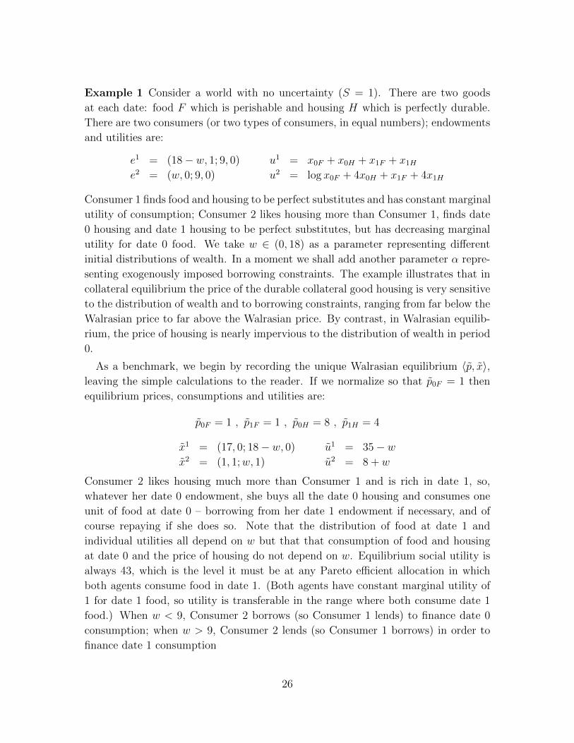
Example 1 Consider a world with no uncertainty (S = 1). There are two goods
at each date: food F which is perishable and housing H which is perfectly durable.
There are two consumers (or two types of consumers, in equal numbers); endowments
and utilities are:
e1 = (18− w, 1; 9, 0) u1 = x0F + x0H + x1F + x1H
e2 = (w, 0; 9, 0) u2 = log x0F + 4x0H + x1F + 4x1H
Consumer 1 finds food and housing to be perfect substitutes and has constant marginal
utility of consumption; Consumer 2 likes housing more than Consumer 1, finds date
0 housing and date 1 housing to be perfect substitutes, but has decreasing marginal
utility for date 0 food. We take w ∈ (0, 18) as a parameter representing different
initial distributions of wealth. In a moment we shall add another parameter α repre-
senting exogenously imposed borrowing constraints. The example illustrates that in
collateral equilibrium the price of the durable collateral good housing is very sensitive
to the distribution of wealth and to borrowing constraints, ranging from far below the
Walrasian price to far above the Walrasian price. By contrast, in Walrasian equilib-
rium, the price of housing is nearly impervious to the distribution of wealth in period
0.
As a benchmark, we begin by recording the unique Walrasian equilibrium 〈p, x〉,leaving the simple calculations to the reader. If we normalize so that p0F = 1 then
equilibrium prices, consumptions and utilities are:
p0F = 1 , p1F = 1 , p0H = 8 , p1H = 4
x1 = (17, 0; 18− w, 0) u1 = 35− wx2 = (1, 1;w, 1) u2 = 8 + w
Consumer 2 likes housing much more than Consumer 1 and is rich in date 1, so,
whatever her date 0 endowment, she buys all the date 0 housing and consumes one
unit of food at date 0 – borrowing from her date 1 endowment if necessary, and of
course repaying if she does so. Note that the distribution of food at date 1 and
individual utilities all depend on w but that that consumption of food and housing
at date 0 and the price of housing do not depend on w. Equilibrium social utility is
always 43, which is the level it must be at any Pareto efficient allocation in which
both agents consume food in date 1. (Both agents have constant marginal utility of
1 for date 1 food, so utility is transferable in the range where both consume date 1
food.) When w < 9, Consumer 2 borrows (so Consumer 1 lends) to finance date 0
consumption; when w > 9, Consumer 2 lends (so Consumer 1 borrows) in order to
finance date 1 consumption
26

In the GEI world, in which securities always deliver precisely what they promise
and security sales do not need to be collateralized, the Walrasian outcome will again
obtain when there are at least as many independent securities as states of nature –
here, at least one security whose payoff is never 0.
However, in the world of collateralized securities, Walrasian outcomes need not
obtain. When w is small, Consumer 2 is poor at date 0 and so would like to borrow
– but the amount she can borrow is constrained by the fact that she will never be
required to repay more than the future value of the collateral. When w is large,
Consumer 2 is rich at date 0 and so would like to lend – but the amount she can lend
is constrained by the fact that the borrower would necessarily need to hold collateral.
Using housing to collateralize its own purchase is leveraging; regulating this lever-
aging can be accomplished by setting collateral requirements. To see the macro-
economic effects of regulating leverage, we introduce another exogenous parameter
α ∈ [0, 4] that specifies the size of the security promise that can be made using
a house as collateral. We assume that only one security (Aα, c) = (αp1F , δ0H) is
available for trade; (Aα, c) promises the value of α units of food in date 1 and is
collateralized by 1 unit of date 0 housing.15 As we shall see the nature of collateral
equilibrium depends on the parameters w, α; Figure 1 depicts the various equilibrium
regions and the price of housing as functions of these parameters. Note that even this
simplest of settings is quite rich.
15In our formulation, the security promise and collateral requirement are specified exogenously
and the security price is determined endogenously. A more familiar formulation would specify the
security price and the down payment requirement exogenously and have the interest rate (hence the
security promise) be determined endogenously. Of course, the two formulations are equivalent: the
down payment requirement d, interest rate r, house price p0H , security price qα and promise α are
related by the obvious equations: d = (p0H − qα)/p0H , r = (α− qα)/qα.
27
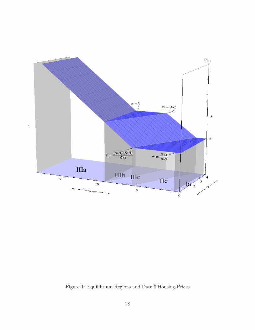
Figure 1: Equilibrium Regions and Date 0 Housing Prices
28

Before beginning the calculations (which are perhaps surprisingly delicate), we
make a useful observation: Increasing α enables Consumer 2 to back more borrowing
with the same collateral and hence to buy more housing with borrowed money.16
Since Consumer 2 loves housing and is rich in the last period, enabling her to borrow
makes her better off, all else equal. But all else need not be equal: when all the
Consumer 2 types borrow, competition will then raise the price of housing. We trace
out the effects of these opposite forces on her welfare by computing equilibrium for
each parameter pair (w, α).
Because we compute equilibria via first order conditions, especially those of Con-
sumer 2, it is convenient to classify equilibria according to the quantity of housing
and the amount of borrowing capacity exercised by Consumer 2; by definition the
borrowing capacity ψ2 cannot exceed housing held, so this leads to 9 potential types
of equilibria, as in Table 1 – but because the collateral requirement entails that
ψ2 ≤ x20H , there are no equilibria of types Ib, Ic so that only 7 types of equilibria are
actually possible.
Table 1: Types of Equilibriumψ2 = 0 0 < ψ2 < x2
0H 0 < ψ2 = x20H
x20H = 0 Ia Ib Ic
x20H ∈ (0, 1) IIa IIb IIc
x20H = 1 IIIa IIIb IIIc
For the given functional forms, we shall see that there are no equilibria of type IIb
(although there would be equilibria of type IIb for some other functional forms and
parameter values). For all the other types, we solve simultaneously for the equilibrium
variables and the region in the parameter space in which an equilibrium of that type
obtains. We find that these regions are disjoint and partition the parameter space,
and that there is a unique equilibrium for each parameter pair (w, α). For many of the
variables, the equilibrium values do not depend on the parameters w, α, and we find
these first; then we sketch the calculations for the remaining equilibrium variables
in types IIc, IIIc, and IIIa, leaving the details and calculations for other types to
the reader. We present quite a lot of detail because the calculations are surprisingly
complicated and illustrate well the notions discussed in Section 4.
To solve for equilibrium, we begin by normalizing (as we are free to do) so that
p0F = 1. Because (Aα, c) is a real security we are also free to normalize so that
16As we shall show, p1H = 4 in every equilibrium, so if α > 4 an agent who sells (Aα, c) will default,
delivery will be 4 rather than α and the resulting equilibrium will coincide with the equilibrium that
would prevail with α = 4.
29

p1F = 1. In collateral equilibrium no agent can begin with less wealth in any state
s ≥ 1 than his inital endowment. At date 1 the prices and allocations that prevail are
those in the standard exchange economy that results after endowments are adjusted
to reflect asset deliveries. It follows that Consumers 1 and 2 each consume food
in date 1 (x11F > 0, x2
1F > 0), that Consumer 2 acquires all the housing at date 1,
(x11H = 0, x2
1H = 1), that the price of housing in period 1 is 4, (p1H = 4) and that
the marginal utilities of money to both agents at date 1 are one (µ11 = µ2
1 = 1).
Because α ∈ [0, 4], the date 1 value of collateral (weakly) exceeds the promise Aα, so
Del(Aα, p) = α; hence MU1(Aα,c)
= MU2(Aα,c)
= α. The marginal utility to Consumer
2 of owning the house in date 0 is obviously 8, since she can live in it at both dates.
The marginal utility to Consumer 1 of owning the house at date 0 is 5, since he can
live in it at date 0 and sell it for 4 units of food in period 1.
We assert that in every equilibrium, no matter who or whether the security is sold,
the security price qα ≥ α. To see this, suppose qα < α. Because Consumer 1’s
marginal utility for food is 1 in both dates, optimality of his equilibrium consumption
means that it must not be possible for him to shift from food consumption to holding
the security, so necessarily x10F = 0. But then x2
0F = 18 so it is possible for Consumer 2
to make this shift; since Consumer 2’s marginal utility for date 0 food is 1/x20F = 1/18
and her marginal utility for date 1 food is 1, this is a contradiction. So we conclude
that qα ≥ α, as asserted.
Next we assert that p0H ≥ 5. If p0H < 5 then Consumer 1 would strictly prefer to
buy date 0 housing rather than date 0 food so optimality implies that x10F = 0. Since
Consumer 1 initially owns the entire housing stock and a strictly positive amount
of date 0 food, he must be spending some of his date 0 income on purchasing the
security at price qα ≥ α, from which (like food) he gets at most one utile per dollar
spent (since µ11 = 1). From this contradiction we conclude that p0H ≥ 5, as asserted.
Finally, we assert that in equilibrium Consumer 1 could never be a net borrower
(sell more of the security than he buys), even in cases where he is very poor in state
0 and Consumer 2 is very rich. If he did, then Consumer 2 would have to be a net
lender, which by the fundamental pricing lemma implies that
1/x20F
1=MU2
0F
p0F
=MU2
(Aα,c)
qα=αµ2
1
qα=
α
qα
or x20F = qα/α ≥ 1. But then from Consumer 2’s optimization involving a positive
amount of food,1/x2
0F
1=MU2
0F
p0F
≥ MU20H
p0H
=8
p0H
which implies that p0H ≥ 8x20F . If Consumer 1 is borrowing, then (since he began
30

with all the housing stock) x10F > 0 and µ1
0 = 1. Moreover, in order to borrow he
must continue to hold housing. He will only desire that if the fundamental value of
the residual from the leveraged purchase of housing is at least as high as its price,
MU10H − αµ1
1 ≥ µ10(p0H − qα)
5− α ≥ p0H − qα ≥ 8x20F − αx2
0F = (8− α)x20F ≥ 8− α
which is a contradiction. Thus Consumer 1 cannot be a net borrower in equilibrium,
and so we can take ψ1 = ϕ2 = 0.
Summarizing: for all w ∈ (0, 18), all α ∈ [0, 4], and in every equilibrium, we have
p0F = 1, p1F = 1, p1H = 4, p0H ≥ 5, qα ≥ α, ψ1 = 0, ϕ2 = 0, µ10 = µ1
1 = µ21 = 1 (5)
Furthermore, if there is trade in the securities market, then Consumer 1 must be the
lender and qα = α.
Lastly we observe that since housing gives higher utility to consumer 2 than to
Consumer 1, and since µ10 = µ1
1 = µ21 = 1, the only way they could both hold housing
at date 0 is if x20F < 1 so that µ2
0 > 1. But in that case, Consumer 2 would borrow
as much as he could using his housing as collateral. This rules out equilibria of type
IIb and also rules out equilibria of type IIa except in the trivial case α = 0.
With these preliminary observations out of the way, we shall proceed through
cases in which Consumer 2 gets progressively richer and the price of housing gets
progressively higher. We begin by analyzing equilibrium of the first interesting type,
IIc, in which Consumer 1 and Consumer 2 both hold housing and Consumer 2 borrows
all he can on his housing. Since Consumer 1 is lending, we showed already that qα = α.
Since Consumer 1 could always buy food, obtaining one utile per dollar expended, and
since he does not have any collateral reason to hold housing, we must have p0H ≤ 5.
Combined with the above demonstration that p0H ≥ 5, we deduce p0H = 5.
To solve for the remaining equilibrium variables we use Consumer 2’s date 0 first
order conditions – but the correct first order conditions may not be obvious. Because
Consumer 2 holds food and housing at date 0, it might appear by analogy with
standard first order conditions that
MU20F
p0F
=MU2
0H
p0H
(6)
MU20F
p0F
=MU2
(Aα,c)
qα(7)
Consumer 2 enjoys 4 utils from living in the house at each date, so MU20H = 8. In
view of our earlier calculations, it follows from (6) that MU20F = 8/5 and from (7)
that MU20F = 1, which is nonsense.
31

The error in this analysis is that (6) and (7) are not the correct first order conditions
for Consumer 2. They neglect the collateral value for housing and the liquidity value
for securities, respectively. Consumer 2 can borrow against date 1 income by selling
the security, but selling the security requires holding collateral. By assumption, at
equilibrium x20H = ψ2, so Consumer 2 is exercising all of her borrowing power; hence
she cannot hold less housing without simultaneously divesting herself of some of the
security and cannot sell more of the security without simultaneously acquiring more
housing.
The correct first order conditions for Consumer 2 derive from the equality between
the fundamental value to Consumer 2 of the residual of the leveraged purchase and
its price. In other words, buying an additional infinitesimal amount ε of housing costs
p0Hε, but of this cost qαε = αε can be borrowed by selling α units of the security, using
the additional housing as collateral, so the net payment is only (p0H − qα)ε = (p0H −α)ε. However, doing this will require repaying the loan in date 1, so the additional
utility obtained will not be MU20Hε = 8ε but rather (MU2
0H −α)ε = (8−α)ε. On the
other hand, selling an additional ε units of food generates income of p0F ε at a utility
cost of MU20F ε. Hence the correct first order condition for Consumer 2 is not (6), but
rather1
x20F
=MU2
0F
p0F
=MU2
0H − αp0H − α
=8− α5− α
(8)
Consumer 2’s date 0 budget constraint is
(5− α)x20H + x2
0F = w (9)
Solving yields
x20F =
5− α8− α
, x20H =
w − 5−α8−α
5− αFrom this we can solve for all the equilibrium consumptions and utilities and security
32
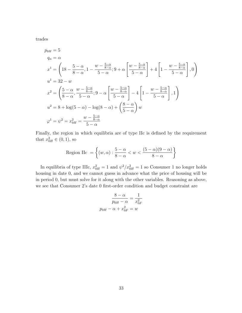
trades
p0H = 5
qα = α
x1 =
(18− 5− α
8− α, 1−
w − 5−α8−α
5− α; 9 + α
[w − 5−α
8−α
5− α
]+ 4
[1−
w − 5−α8−α
5− α
], 0
)u1 = 32− w
x2 =
(5− α8− α
,w − 5−α
8−α
5− α; 9− α
[w − 5−α
8−α
5− α
]− 4
[1−
w − 5−α8−α
5− α
], 1
)
u2 = 8 + log(5− α)− log(8− α) +
(8− α5− α
)w
ϕ1 = ψ2 = x20H =
w − 5−α8−α
5− α
Finally, the region in which equilibria are of type IIc is defined by the requirement
that x20H ∈ (0, 1), so
Region IIc =
{(w, α) :
5− α8− α
< w <(5− α)(9− α)
8− α
}In equilibria of type IIIc, x2
0H = 1 and ψ2/x20H = 1 so Consumer 1 no longer holds
housing in date 0, and we cannot guess in advance what the price of housing will be
in period 0, but must solve for it along with the other variables. Reasoning as above,
we see that Consumer 2’s date 0 first-order condition and budget constraint are
8− αp0H − α
=1
x20F
p0H − α + x20F = w
33

Solving yields:
p0H = α +
(8− α9− α
)w
qα = α
x1 =
(18− w
9− α, 0; 9 + α, 0
)u1 = 27 + α− w
9− α
x2 =
(w
9− α, 1; 9− α, 1
)u2 = log
(w
9− α
)+ 17− α
ϕ1 = ψ2 = x20H = 1
The region in which equilibria are of type IIIc is determined by the requirements
that it be optimal for Consumer 2 to borrow the maximum amount possible, whence
x0F ≤ 1, and that Consumer 1 not wish to buy housing, whence p0H ≥ 5. Putting
these together yields:
Region IIIc =
{(w, α) :
(5− α8− α
)(9− α) ≤ w ≤ (9− α)
}In region IIIa, the security is not traded but Consumer 2 holds all the housing and
some food at date 0, so Consumer 2 must be rich enough at date 0 to buy all the
housing without borrowing, and must be indifferent to trading date 0 food for date 0
housing or for the security. Her first order conditions and budget constraint at date
0 are:
MU2(A,c)
qα=MU2
0F
p0F
(10)
MU20F
p0F
=MU2
0H
p0H
(11)
1 · x20F + p0H · 1 = w (12)
Solving yields
p0H =8w
9, x2
0F =w
9, qα =
αw
9
At these prices, Consumer 1 would like to sell the security, but is deterred from doing
so by the requirement to hold (expensive) collateral. Equilibrium consumptions and
34

utilities are:
x1 = (26− w, 0; 9, 0)
u1 = 35− w
x2 = (w
9, 1; 9, 1)
u2 = log(w
9
)+ 17
ϕ1 = ψ2 = 0
Finally, region IIIa is defined by the requirement that Consumer 2 be rich enough to
buy all the housing at date 0:
Region IIIa = {w : w ≥ 9}
We summarize the description of equilibrium in the remaining regions Ia, IIa, and
IIb below.
• Ia 0 < w ≤ (5− α)/(8− α)
p0H = 5
qα = α
x1 = (18− w, 1; 13, 0)
u1 = 32− wx2 = (w, 0; 5, 1)
u2 = logw + 9
ϕ1 = ψ2 = 0
• IIa α = 0, 5/8 < w < 45/8
p0H = 5
qα = α
x1 =
(18− 5
8, 1− (
w
5− 1
8); 13− 4(
w
5− 1
8), 0
)u1 = 32− w
x2 =
(5
8,w
5− 1
8; 5 + (
w
5− 1
8), 1
)u2 = log(
5
8) + 8 +
8w
5
ϕ1 = ψ2 = 0
35

• IIIb 9− α < w < 9
p0H = 8
qα = α
x1 = (17, 0; 18− w, 0)
u1 = 35− wx2 = (1, 1;w, 1)
u2 = 8 + w
ϕ1 = ψ2 =9− wα
Example 1 reinforces a number of the points made in Section 4.
• In Walrasian equilibrium the price of housing p0H = 8 no matter what the
distribution of income in period 0. If Consumer 2 is poor in period 0, she borrows
against her big income in period 1. By contrast, in collateral equilibrium, the
price of housing rises from p0H = 5 to p0H = 16 as w rises from 0 to 18. The
price of housing also rises when α rises, that is, when more borrowing is allowed.
In this example, asset prices are much more volatile in collateral equilibrium
than in Walrasian equilibrium.
• CE allocations may be inefficient – and in particular, differ from Walrasian
allocations – even when financial markets are “complete.” Because Example 1
represents a transferable utility economy, an allocation is Pareto efficient if and
only if the sum of individual utilities is 43; these allocations are precisely those
for which Consumer 2 holds all the housing in both dates and exactly one unit of
date 0 food: x20H = x2
1H = 1 and x20F = 1. Hence, CE is Pareto efficient exactly
when w ∈ [9−α, 9]; that is, in Region IIIb and in portions of the boundaries of
Regions IIIa and IIIc. And, as asserted in Theorem 3, wherever CE is efficient,
it is equivalent to WE.
• For w 6∈ [5, 9] collateral equilibrium is inefficient no matter what collateral re-
quirement is set; indeed, collateral equilibrium will be inefficient no matter what
collateralized securities are available for trade. (See [Geanakoplos and Zame, 2010],
Theorem 3).
• As asserted in Theorem 2, in every region where CE 6= GEI, there are distortions
and some consumer experiences a collateral value and liquidity value. In Regions
IIc and IIIc this is Consumer 2. To see the distortions more concretely, fix
36
w = 7/2. For α ∈ (0, 2) parameter values are in region IIc and for α ∈ [2, 4]
parameter values are in region IIIc but in both cases the collateral requirement
distorts Consumer 2’s consumption choice, leading her to hold “too much”
housing, given the price. To see this, compare marginal utilities per dollar
for date 0 food and date 0 housing. In Region IIc we have
MU20F
p0F
=8− α5− α
>8
5=MU2
0H
p0H
while in Region IIIc we have
MU20F
p0F
=2(9− α)
7>
16
7(α + 8−α9−α)
=MU2
0H
p0H
This distortion can be seen in prices as well: to say that Consumer 2’s marginal
utility per dollar for date 0 food exceeds her marginal utility per dollar for date
0 housing is to say that the price of date 0 housing is too high. Consumer 2
is willing to pay the higher price of date 0 housing because holding housing
enables her to borrow; that is, she derives a collateral value from housing as
well as a consumption value. Similarly, Consumer 2 finds the marginal utility
per dollar for date 0 food to be higher than the marginal utility of making the
payments on the security; the price of the security is “too high” as well – she
experiences a liquidity value.
In the portion of Region IIIa where w > 9, it is Consumer 1 who experiences
collateral values and a liquidity value, although Consumer 1 neither holds hous-
ing nor sells the security. In this region, at the prevailing interest rate (asset
price), Consumer 1 would be delighted to borrow (sell the asset) but is discour-
aged from doing so because he would have to hold collateral, which he does not
wish to do. In this region the effect of the collateral distortion is to shut down
the borrowing/lending market entirely.
• The effects of collateral requirements on welfare are subtle. Again, fix w = 7/2.
Increases in α (equivalently, decreases in the down payment requirement) make
it possible for consumers of type 2 to access more date 1 wealth. For α ∈ [0, 2),
this makes it possible for consumers of type 2 to afford more housing; the net
result is Pareto improving. For α ∈ [2, 4], however, consumers of type 2 already
own all the available houses, so increasing α only leads to more competition
among them, which serves only to drive up the price of date 0 housing (from
p0H = 5 when α = 2 to p0H = 34/5 when α = 4). This price increase makes
Consumers of type 1 better off but makes Consumers of type 2 worse off.
37

• In this Example, we insisted that only one security is offered, a mortgage collat-
eralized by a single house and promising the value of α units of food. However,
nothing would change if we allowed for various mortgages, each collateralized
by a single house (this is just a normalization) but with different promises. The
reason is that only the security with the largest liquidity value will be traded;
this is the (unique) mortgage with the largest promise.
6 Default, Crashes and Welfare
Default and crashes are suggestive of inefficiency. As the Examples presented in
this Section show, this need not be true: both default and crashes may be welfare
enhancing.17 Indeed, as Example 2 shows, levels of collateral that are socially optimal
may lead to default with positive probability.
More generally, there is a link between collateral requirements and future prices.
Lower collateral requirements lead buyers to take on more debt; the difficulties of
servicing this debt can lead to reduced demand and lower prices – and even to crashes
– in the future. Importantly, such crashes occur precisely because lower collateral
requirements encourage borrowers to take on more debt than they can service. And
yet, despite these crashes, lower collateral requirements may be welfare enhancing.
A final point made by these Examples is that although the set of securities available
for trade is given exogenously as part of the data of the model, the set of securities
that are actually traded is determined endogenously at equilibrium. Thus, we may
view the financial structure of the economy as chosen by the competitive market.
As Example 3 shows, if many collateral levels are available, the market may choose
levels of collateral that lead to default with positive probability, and this choice may
be efficient; morever, even if all possible securities are available for trade, the market
may choose an incomplete set to actually be traded at equilibrium.
Example 2 (Default and Crashes) We construct a variant on Example 1. Rather
than present a full-blown analysis as in Example 1, we fix endowments and take only
the security promise as a parameter, making it easier to focus on the points of interest.
There are two states of nature and two goods: Food, which is perishable, and
Housing, which is durable. There are two (types of) consumers, with endowments
17That default may be welfare enhancing is a point that has been made, in different contexts, by
[Zame, 1993], [Sabarwal, 2003] and [Dubey et al., 2005].
38

and utility functions:
e1 = (29/2, 1; 9, 0; 9, 0)
u1 = x0F + x0H + (1/2)(x1F + x1H) + (1/2)(x2F + 3x2H)
e2 = (7/2, 0; 9, 0; 5/2, 0)
u2 = log x0F + 4x0H + (1/2)(x1F + 4x1H) + (1/2)(x2F + 4x2H)
Note the only differences from Example 1 are that Consumer 1 likes housing better
in state 2 and Consumer 2 is poor in state 2 – the ‘bad’ state.
A single security – a mortgage – Aα = (αp1F , αp2F ; δ0H), promising the value of α
units of food and collateralized by 1 unit of housing, is available for trade; we take
α ∈ [0, 4] as a parameter.18 (Equivalently, we could consider securities that promise
to deliver the value of one unit of food and are collateralized by 1/α units of housing.)
We distinguish four regions; in each there is a unique equilibrium. In Region I, α is
sufficiently small that Consumer 2 cannot borrow enough to buy all the housing at
date 0, but buys the remaining housing in date 1. In Region II, α is large enough that
Consumer 2 can buy all the housing at date 0 but small enough that she will be able
to honor her promises in both states at date 1 and retain all the housing at date 1. In
Region III, Consumer 2 will honor her promises but will not be able to retain all the
housing. In Region IV, Consumer 2 will default. Finally, at the boundary of Regions
II and III, prices and equilibrium consumptions are indeterminate. The calculations
in Regions I, II are almost identical to those in Example 1; the calculations for Regions
III, IV follow the same method with the appropriate changes to incorporate default.
In all regions we can take the price of food to be 1 in every state s = 0, 1, 2.
• Region I: α ∈ [0,2)
Consumers 1 and 2 both hold date 0 housing; Consumer 2 borrows as much as
she can in date 0 and honors her promises in both states at date 1. In both
states at date 1, Consumer 2 buys the remaining housing out of her remaining
balance of food. Hence the price of housing in both states is 4, and the marginal
utility of a dollar to each consumer is 1 in both states. It follows that qα = α,
and that p0H = 5. The key equations are the marginal condition for Consumer
2 on the residual from the leveraged purchase of the house and the budget
equation that says that all income not spent on food must be spent on housing:
1/x20F
p0F
=8− α5− α
⇒ x20F =
5− α8− α
x20H =
7/2− 5−α8−α + αx2
0H
518As before, the case α > 4 reduces to the case α = 4.
39

Solving yields
x20H = 1− 7
2(5− α)+
1
8− αHence equilibrium prices and consumptions are:
p = (1, 5; 1, 4; 1, 4)
x1 =
(18− 5− α
8− α, 1− x2
0H ; 13 + (α− 4)x20H , 0 ; 13 + (α− 4)x2
0H , 0
)x2 =
(5− α8− α
, x20H ; 5− (α− 4)x2
0H , 1 ;−3
2− (α− 4)x2
0H , 1
)(Lest date 1 food consumptions seem strange, remember that (α−4) < 0.) As α
increases (the collateral requirement becomes less stringent) in this range, there
is no effect on date 0 housing prices p0H = 5 but Consumer 2 is able to borrow
more which also gives her an incentive to shift date 0 consumption from food
to housing, so her date 0 food consumption decreases and her date 0 housing
consumption increases: x20F = 5/8, x2
0H = 23/40 when α = 0; x20F = 1/2, x2
0H =
1 when α = 2.
• Region II: α ∈ [2,5/2)
Consumer 2 holds all the housing at both dates; Consumer 2 borrows as much
as she can in date 0 and honors her promises in both states at date 1. Again
the two key equations are:
1/x20F
p0F
=8− αp0H − α
⇒ x20F =
p0H − α8− α
p0H = 7/2− p0H − α8− α
+ α
Equilibrium prices and consumptions are:
p =
(1, α +
(8− α9− α
)(7
2
); 1, 4; 1, 4
)qα = α
x1 =
(18− 7
2(9− α), 0; 9 + α, 0; 9 + α, 0
)x2 =
(7
2(9− α), 1; 9− α, 1;
5
2− α, 1
)As α increases in this range, date 0 housing prices rise but Consumer 2 is
able to borrow more; she is already holding all the housing at date 0 but can
now consume more food as well: x20F = 1/2, x2
0H = 1, p0H = 5 when α = 2,
x20F = 7/13, x2
0H = 1, p0H = 71/13 in the limit as α→ 2.5.
40

• Boundary between Regions II, III: α = 5/2
Consumer 2 holds all the housing at both dates; Consumer 2 borrows as much
as she can in date 0; Consumer 2 honors her promises in both states at date
1. In the bad state, Consumer 2 holds all the housing and no food so p2H is
indeterminate. This makes the crucial equations a bit more complicated, also
because µ22 = 4/p2H
1/x20F
p0F
=4 + .5(4− α) + .5(p2H − α) 4
p2H
p0H − α⇒ x2
0F =p0H − α
8− (.5 + 2p2H
)α
p0H = 7/2− p0H − α8− (.5 + 2
p2H)α
+ α
This gives
p0H = α +7
2
8− (.5 + 2p2H
)α
9− (.5 + 2p2H
)α=
5
2+
7
2
27/4− 5p2H
31/4− 5p2H
x20F =
7
2
1
9− (.5 + 2p2H
)α=
7
2
1
31/4− 5p2H
Notice that as p2H falls (in its indeterminate range), x20F rises and p0H falls.
Equilibrium prices and consumptions are:
p =
(1,
5
2+
(7
2
)(27p2H − 20
31p2H − 20
); 1, 4; 1, p2H
)p2H ∈ [3, 4]
qα = 5/2
x1 =
(18− 14p2H
31p2H − 20, 0;
23
2, 0;
23
2, 0
)x2 =
(14p2H
31p2H − 20, 1;
13
2, 1; 0, 1
)When α = 5/2 date 0 food consumption is indeterminate at equilibrium but
all other consumptions are determinate. For the equilibrium with p2H = 4
(which is the limit of equilibria as α converges to 5/2 from below), x10F =
317/13, x20F = 7/13, p0H = 71/13; for the equilibrium with p2H = 3 (which is
the limit of equilibria as α converges to 5/2 from above), x10F = 1272/73, x2
0F =
42/73, p0H = 396/73. Hence Consumer 1 is better off “just before” the crash
and Consumer 2 is better off “just after” the crash. Total utility is higher “just
after” the crash,
41

• Region III: α ∈ (52,3]
Consumer 2 holds all the housing at date 0; Consumer 2 borrows as much as she
can in date 0; Consumer 2 honors her promises in the good state at date 1. In
the bad state the price of housing falls to p2H = 3; Consumer 2 (who has assets
of endowment plus housing = (5/2) + 3) sells the house, repays her debt, and
then buys all the housing she can afford at the price p2H = 3; Consumer 1 holds
the remaining housing. The crucial equations are now a bit more complicated
because p2H = 3 and µ22 = 4/3:
1/x20F
p0F
=4 + .5(4− α) + .5(3− α)4
3
p0H − α=⇒ x2
0F =p0H − α8− 7
6α
p0H = 7/2− p0H − α8− 7
6α
+ α
Equilibrium prices and consumptions are:
p =
(1, α +
(7
2
)(48− 7α
54− 7α
); 1, 4, 1, 3
)qα = α
x1 =
(18− 21
54− 7α, 0; 9 + α, 0;
23
2,2α− 5
6
)x2 =
(21
54− 7α, 1; 9− α, 1; 0,
11− 2α
6
)As α increases in this range, date 0 housing prices rise again but Consumer 2
is again able to borrow more and her consumption of date 0 food rises: p0H =
396/73, x20F = 42/73 when α = 5
2, p0H = 129/22, x2
0F = 7/11 when α = 3.
• Region IV α ∈ (3,4]
Consumer 2 holds all the housing at date 0; Consumer 2 borrows as much as
she can in date 0; Consumer 2 honors her promises in the good state at date
1. In the bad state the price of housing falls to p2H = 3; Consumer 2, who
has assets of endowment plus housing = (5/2) + 3, delivers the house (which is
worth 3) instead of her promise (which is α > 3), defaults on her debt, and then
buys all the housing she can afford at the price p2H = 3; Consumer 1 holds the
remaining housing. Now the price of debt is qα = (.5α + .5(3)) and the crucial
equilibrium equations are
1/x20F
p0F
=4 + .5(4− α) + .5(3− 3)4
3
p0H − qα⇒ x2
0F =p0H − 1.5− α/2
6− α/2
p0H = 7/2− p0H − 1.5− α/26− α/2
+ .5α + 1.5 = 5− p0H − 1.5− α/26− α/2
+ α/2
42

These give
(7− α/2)(p0H − α/2) = 5(6− α/2) + 1.5 = 63/2− 5α/2
p0H =63/2− 5α/2
7− α/2+ α/2 =
63− 5α
14− α+ α/2
x20F =
63−5α14−α − 1.5
6− α/2=
42−3.5α14−α
6− α/2=
84− 7α
(14− α)(12− α)=
7
14− α
Equilibrium prices and consumptions are:
p =
(1,α
2+
(63− 5α
14− α
); 1, 4; 1, 3
)qα =
α + 3
2
x1 =
(29
2−(
7
14− α
), 0; 9 + α, 0;
23
2,1
6
)x2 =
(7
14− α, 1; 9− α, 1; 0,
5
6
)After default, the date 0 housing price and Consumer 2’s date 0 food consump-
tion rise: p0H = 129/22, x20F = 7/11 when α = 3 and p0H = 63/10, x2
0F = 7/10
when α = 4.
We want to make two very important points about this example:
• As α rises past α = 5/2 the price of housing in the bad state falls precipitously
from 4 to 3: there is a crash. The crash occurs despite the fact that all agents
are perfectly rational, have perfect foresight and hold the same beliefs: the low
collateral requirement (equivalently low down payment requirement) provides
incentive for consumers of type 2 to take on more debt than they can service.
Strikingly, the crash occurs when α < 3 – before consumers of type 2 default on
their promises. Perfect foresight entails that the crash is rationally anticipated,
so it leads to a sudden drop in the price of housing at date 0, from 71/13 = 5.46
to 396/73 = 5.42.
• As in Example 1 this is a transferable utility economy (Consumers 1 and 2
have constant and equal marginal utilities for food in the good state 1), so we
may identify social welfare with the sum of individual utilities. The effects of
collateral requirement on welfare are complicated; direct computation shows
that there are a number of different regimes:
43

– 0 ≤ α < 2: welfare of both types of consumers is increasing; social welfare
is increasing
– 2 < α ≤ 5/2: welfare of consumers of type 1 is increasing, welfare of con-
sumers of type 2 is decreasing; social welfare is decreasing
– α = 5/2: welfare of consumers of type 1 jumps down, welfare of consumers
of type 2 jumps up; social welfare jumps up
– 5/2 < α ≤ 3: welfare of consumers of type 1 is increasing, welfare of con-
sumers of type 2 is decreasing; social welfare is decreasing
– 3 < α ≤ 4: welfare of consumers of type 1 is increasing, welfare of con-
sumers of type 2 is decreasing; social welfare is increasing
In particular, social welfare is higher after the crash than immediately before,
and social welfare is higher after default than immediately before, so collateral
levels that lead to a perfectly foreseen crash or to perfectly foreseen default can
be welfare enhancing. It is thus hasty to presume that default and crashes are,
all things considered, destructive to welfare.
In our framework, the set of securities available for trade is given exogenously,
but the set actually traded is determined endogenously at equilibrium. Because the
former set might be very large (conceptually, all conceivable securities) we can view
the security market structure itself as determined by the action of the competitive
market. As we see below, the result can be default at equilibrium (even when securities
that do not lead to default are available for trade).
Example 3 (Which Securities are Traded?) We maintain the entire structure
of Example 2, except that some arbitrary set {(Aj, cj)} of securities is available for
trade. To be consistent with our framework, we assume the set of available securities
is finite, but, at least conceptually, we might imagine that all possible securities are
offered. Because only housing is durable, we assume that only housing is used as
collateral; there is no loss in normalizing so that cj = δ0H for each j.
In this setting, only Consumer 2 will sell securities (borrow); as Theorem 1 showed,
Consumer 2 will sell only that security which offers her the largest liquidity value.
(If more than one security offers Consumer 2 the largest liquidity value, Consumer 2
might sell any or all of them.) To see this, suppose that at equilibrium Consumer 2
sells (Aj, cj) but that LV 2(Ak,ck)
> LV 2(Aj ,cj). Because both securities require the same
collateral Consumer 2 could sell ε fewer shares of (Aj, cj) and ε more shares of (Ak, ck)
without violating her collateral constraint. The definition of liquidity value means
44

that this change would strictly improve Consumer 2’s utility, which would contradict
the requirement that Consumer 2 optimizes at equilibrium.
Because liquidity values depend on the equilibrium prices and consumptions, it is
not in general possible to order a priori the liquidity values of given securities and
hence to know which securities will be traded and which will not be. Instead, we
analyze two particularly interesting scenarios.
Suppose first that mortgages with various promises – but no other securities –
are available. As above, write Aα = (αp1F , αp2F ; δ0H). We claim that only the
mortgage with the greatest promise (not exceeding 4 – the maximum value of housing
in date 1, hence the maximum delivery that will be made on any security) will be
traded at equilibrium. To show this it suffices to show that if α < β ≤ 4 then
LVα = LV 2Aα
< LV 2Aβ
= LVβ. To this end, we estimate marginal utilities of income µ2s
in the various spots, then fundamental values, security prices, then liquidity values.
• In state 1, prices are p1F = 1, p1H = 4 so µ21 = (1/2)1. In state 2, prices are
p2F = 1, p2H ≥ 3 so µ22 ≤ (1/2)4/3. We claim that µ2
0 > 7/6. To see this, note
that µ20 is at least as high as the maximum of marginal utility per dollar for
food and marginal utility per dollar for housing. The former strictly exceeds
7/6 unless x20F ≥ 6/7 and the latter weakly exceeds 8/5 if x2
0H < 1, in which
case p0H = 5. Hence to establish that µ20 > 7/6 it remains only to consider the
case in which x20F ≥ 6/7 and x2
0H = 1. In this case, we have
p0H = p0Hx20H ≤
7
2+ 4− x2
0F ≤15
2− 6
7=
93
14
so that the marginal utility per dollar for housing is at least 8/(93/14) =
112/93 > 7/6, as asserted.
• Because only Consumer 1 buys securities, security prices coincide with expected
actual deliveries. Write αs, βs for the deliveries Aα,Aβ in state s so prices are
qα = (1/2)(α1 + α2) and qβ = (1/2)(β1 + β2).
• We have shown above that µ20 > 7/6, and that µ2
1 = 1/2 and µ22 ≤ 2/3. Using
these estimates and the definitions, we obtain
µ20(LVβ − LVα) = [µ2
0qβ − (µ21β1 + µ2
2β2)]− [µ20qα − (µ2
1α1 + µ22α2)]
= [µ20(β1 + β2)/2− (µ2
1β1 + µ22β2)]− [µ2
0(α1 + α2)/2− (µ21α1 + µ2
2α2)]
= [(µ20/2)− µ2
1][β1 − α1] + [(µ20/2)− µ2
2][β2 − α2]
> (1/12)(β1 − α1)− (1/12)(β2 − α2)
45

Because the delivery on any security will be the minimum of its promise and
the value of collateral it follows that β1 − α1 = β − α and β2 − α2 ≤ β − α.
Hence µ20(LVβ − LVα) > 0, whence LVβ − LVα > 0, as asserted.
In particular, if A4 – the mortgage with the largest promise – is offered, then only
this mortgage will be traded, even though this leads to default in equilibrium.
Now suppose that all possible securities are offered. We assert that in equilib-
rium only those securities (with collateral δ0H) whose deliveries are 4 in state 1
and 3 in state 2 will actually be traded, and that equilibrium commodity prices
and consumptions coincide with the equilibrium when only the security A4 above is
traded. To see this fix an equilibrium. First suppose the security B is traded and
that Del(B, 1, p) < 4. Let B′ be any security with the same collateral and state 2
promise (hence delivery) as B, but which promises (hence delivers) 4 units of account
in state 1. Arguing exactly as above, we see that B′ offers Consumer 2 (the only seller
of B) a strictly greater liquidity value than does B. Hence Consumer 2 would strictly
prefer to sell B′ rather than B, which would be a contradiction. We conclude that if
B is traded then Del(B, 1, p) = 4. Now suppose two securities B,B′ are traded, that
Del(B, 1, p) = Del(B′, 1, p) = 4 but that β2 = Del(B, 2, p) < Del(B′, 2, p) = β′2.
Arguing as before, we see that Consumer 2’s date 0 first-order conditions require:
8− 12(4)− µ2
2(β2)
p0H − 12(4 + β2)
=1
x0F
=8− 1
2(4)− µ2
2(β′2)
p0H − 12(4 + β′2)
However, this would entail β2 = β′2 which would be a contradiction. We conclude
that all securities traded at equilibrium deliver 4 in state 1 and some common β ≤ 4
in state 2.
Finally, consider the magnitude of β. If β > 3 we could argue exactly as in Example
2 to show that default would occur in state 2, which would entail that p2H = 3, and
hence that actual delivery would be only 3 – a contradiction. If β < 2.5 we could argue
as before to show that the equilibrium price p2H = 4, and hence that any security
whose delivery is 4 in state 1 and β′ ∈ (β, 3) in state 2 would offer Consumer 2 a
greater liquidity value which would be a contradiction. If 2.5 ≤ β < 3 the argument
is a little more delicate, in part because the price p2H might be indeterminate in the
interval [3, 4], but the conclusion would be the same: any security whose delivery is 4
in state 1 and β′ ∈ (β, 3) in state 2 would offer Consumer 2 a greater liquidity value,
which again would be a contradiction.
To see the last assertion, note first that if 2.5 ≤ β < 3 then Consumer 2’s behavior
is the same as in Example 2: at date 0 she borrows as much as she can to buy all
the housing; in the good state she delivers the full promise of 4 from her endowment,
46

and holds all the housing; in the bad state she delivers the promise of β from her
endowment of 5/2 and the value p2H of the housing she owns, and uses the remainder
of her wealth to buy back as much housing as she can. If β > 2.5 she cannot buy back
all the housing so Consumer 1 buys some of it, whence p2H = 3; if β = 2.5 the price
of housing is indeterminate: p2H ∈ [3, 4]. As in Example 2, equilibrium is defined by
Consumer 2’s first order conditions and budget constraints; this yields the equations:
1
x20F
=4 + (1/2)[(4− 4) + (p2H − β)(4/p2H)]
p0H − q
p0Fx20F + p0Hx
20H = (7/2) + qx2
0H
where q is the security price. Since the security delivers 4 in the good state and β in
the bad state its price is q = (1/2)(4 + β). We have normalized p0F = 1; consumer 2
buys all the housing at date 0 so x20H = 1. Plugging all these in gives
1
x20F
=6− (2β/p2H)
p0H − (1/2)(4 + β)
x20F + p0H = (7/2) + (1/2)(4 + β)
Solving the second equation for p0H , plugging into the first equation and then solving
yields
x20F =
(7/2)
7− (2β/p2H)
1
x20F
= (2/7)[7− (2β/p2H)]
Since β ∈ [2.5, 3) and p2H ∈ [3, 4] it follows 1/x20F > 10/7. Because µ2
0 ≥ 1/x20F it
follows that µ20 > 10/7 as well. Now we can argue as before to see that any security
that delivers 4 in state 1 and β′ ∈ (β, 3) in state 2 would yield Consumer 2 a higher
liquidity value; since this is a contradiction, we conclude that β = 3, as asserted.
We conclude that only those securities (with collateral δ0H) whose deliveries are
4 in state 1 and 3 in state 2 will actually be traded. It follows immediately that
equilibrium commodity prices and consumptions coincide with the equilibrium when
only the security A4 (see Example 2) is traded.
Note that even though all possible securities are available, the set of securities
that are traded at equilibrium is endogenously incomplete. Note in particular that
Arrow securities are not traded, even though they are available, because they make
extremely inefficient use of the available collateral.
47

7 Is the Security Market Efficient?
In the scenario analyzed in Example 3, the market chooses socially efficient promises
– even though those promises may lead to default. Characterizing situations when
the market does or does not choose socially efficient sets of securities – or at least
Pareto undominated sets of securities – seems an important and difficult question, to
which we do not know the answer. (Indeed, because multiple equilibria are possible,
it is not entirely clear precisely how to formulate the question.) However, we can give
an unambiguous answer about Pareto domination in at least one important case: if
date 1 prices do not depend on the choices of securities.
Theorem 4 (Constrained Efficiency) Every set of collateral equilibrium plans is
Pareto undominated among all sets of plans that:
(a) are socially feasible
(b) given date 0 decisions, respect each consumer’s budget set at every state s at
date 1 at the given equilibrium prices
(c) call for deliveries on securities that are the minimum of the promise and the
value of collateral
Proof Let 〈p, q, (xi, ϕi, ψi)〉 be an equilibrium, and suppose that (xi, ϕi, ψi) is a
family of plans meeting the given conditions that Pareto dominates the equilibrium
set of plans. By assumption, all the alternative plans are feasible, meet the budget
constraints at each state at date 1, and call for deliveries that are the minumum of
promises and the value of collateral, Optimality of the equilibrium plans at prices p, q
means, therefore, that all the alternative plans (xi, ϕi, ψi) fail the budget constraints
at date 0. Because the alternative set of plans is socially feasible, summing over
consumers yields a contradiction.
A particular implication of constrained efficiency is that prohibiting trade in certain
securities – for example, those that are leveraged above some threshold – cannot
lead to a Pareto improvement if it does not lead to a change in date 1 prices. Put
differently: among security structures that lead to the same date 1 prices, the market
chooses efficiently. In an environment or model in which only one good is available for
consumption at date 1 and the price of that good is taken to be 1, it is tautological
that all security structures lead to the same date 1 prices, so in that situation collateral
48

equilibrium will always be constrained efficient and the market will always choose the
security structure efficiently; compare [Kilenthong, 2006].19
8 Conclusion
Collateral requirements are almost omnipresent in modern economies, but the effects
of these collateral requirements have received little attention except in circumstances
where there is actual default. This paper argues that collateral requirements have
important effects on every aspect of the economy – even when there is no default.
Collateral requirements inhibit lending, limit borrowing, and distort consumption
decisions.
When all borrowing must be collateralized, the supply of collateral becomes an
important financial constraint. If collateral is in short supply the necessity of using
collateral to back promises creates incentives to create collateral and to stretch ex-
isting collateral. The state can (effectively) create collateral by issuing bonds that
can be used as collateral and by promulgating law and regulation that make it easier
to seize goods used as collateral.20 The market’s attempts to stretch collateral have
driven much of the financial engineering that has rapidly accelerated over the last
three-and-a-half decades (beginning with the introduction of mortgage-backed secu-
rities in the early 1970’s) and that has been designed specifically to stretch collateral
by making it possible for the same collateral to be used several times: allowing agents
to collateralize their promises with other agents’ promises (pyramiding) and allowing
the same collateral to back many different promises (tranching). These two innova-
tions are at the bottom of the securitization and derivatives boom on Wall Street,
and have greatly expanded the scope of financial markets. We address many of these
issues in a companion paper [Geanakoplos and Zame, 2010] that expands the model
presented here to allow for pyramiding, pooling and tranching. That work charac-
terizes those efficient allocations that can be supported in equilibrium when financial
innovation is possible but borrowing must be collateralized; a central finding is that
robust inefficiency is an inescapable possibility.
The model offered here abstracts away from transaction costs, informational asym-
19Note that constrained efficiency continues to hold even if we add the possibility of instantaneous
production, as discussed in Subsection 4.2. Thus although the market may lead investors to produce
technologically inferior goods – because of their collateral value – this production will be in the social
interest, given the set of possible goods that can be used as collateral, and provided that period 1
prices are not affected.20Similarly, state regulations concerning seizure can have an enormous influence on bankruptcies;
see [Lin and White, 2001] and [Fay et al., 2002] for instance.
49

metries and many other frictions that play an important role in real markets. It also
restricts attention to a two-date world, and so does not address issues such as default
at intermediate dates. All these are important questions for later work.
50

References
[Araujo et al., 2005] Araujo, A., Fajardo, J., and Pascoa, M. (2005). Endogenous
collateral. Journal of Mathematical Economics, 41:439–462.
[Araujo et al., 2002] Araujo, A., Pascoa, M., and Torres-Martinez, J. (2002). Collat-
eral avoids Ponzi schemes in incomplete markets. Econometrica, 70:1613–1638.
[Bernanke et al., 1996] Bernanke, B., Gertler, M., and Gilchrist, S. (1996). The fi-
nancial accelerator and the flight to quality. Review of Economics and Statistics,
78:1–15.
[Debreu, 1959] Debreu, G. (1959). Theory of Value. Yale University Press, New
Haven.
[Dubey et al., 2005] Dubey, P., Geanakoplos, J., and Shubik, M. (2005). Default and
punishment in a general equilibrium model with incomplete markets. Econometrica,
73:1–37.
[Dubey et al., 1995] Dubey, P., Geanakoplos, J., and Zame, W. R. (1995). Collateral,
default and market crashes. Cowles Foundation Discussion Paper.
[Duffie and Shafer, 1985] Duffie, D. and Shafer, W. (1985). Equilibrium in incomplete
markets, I: A basic model of generic existence. Journal of Mathematical Economics,
14:285–300.
[Duffie and Shafer, 1986] Duffie, D. and Shafer, W. (1986). Equilibrium in incomplete
markets, II: Generic existence in stochastic economies. Journal of Mathematical
Economics, 15:199–216.
[Elul, 1999] Elul, R. (1999). Effectively complete equilibria – a note. Journal of
Mathematical Economics, 32:113–119.
[Elul, 2005] Elul, R. (2005). The economics of asset securitization. Federal Reserve
Bank of Philadalphia Business Review, pages 16–25.
[Fay et al., 2002] Fay, S., Hurst, E., and White, M. (2002). The household
bankruptcy decision. American Economic Review, 92:706–718.
[Fostel and Geanakoplos, 2008] Fostel, A. and Geanakoplos, J. (2008). Leverage cy-
cles and the anxious economy. American Economic Review, 98:1211–1244.
51
[Geanakoplos, 1997] Geanakoplos, J. (1997). Promises, promises. In W.B. Arthur,
et al., editor, The Economy as an Evolving Complex System, II. Addison-Wesley,
Reading, MA.
[Geanakoplos, 2003] Geanakoplos, J. (2003). Liquidity, default and crashes: En-
dogenous contracts in general equilibrium. In Eighth World Econometric Society
Conference, Vol. II, pages 170–205. Econometric Society Monographs.
[Geanakoplos and Zame, 2010] Geanakoplos, J. and Zame, W. R. (2010). Securitiza-
tion and tranching. Technical report, UCLA.
[Girardi et al., 2008] Girardi, K., Shapiro, A., and Willen, P. (2008). Subprime out-
comes: Risky mortgages, homeownership experiences, and foreclosures. Federal
Reserve Bank of Boston Working Paper.
[Hart, 1975] Hart, O. (1975). On the optimality of equilibrium when the market
structure is incomplete. Journal of Economic Theory, 11:418–443.
[Hellwig, 1981] Hellwig, M. F. (1981). Bankruptcy, limited liability and the
Modigliani-Miller theorem. American Economic Review, 72:155–170.
[Holmstrom and Tirole, 1997] Holmstrom, B. and Tirole, J. (1997). Financial inter-
mediation, loanable funds and the real sector. Quarterly Journal of Economics,
112:663–692.
[Kau et al., 1994] Kau, J., Keenan, D., and Kim, T. (1994). Default probabilities for
mortgages. Journal of Urban Economics, 35:278–296.
[Kehoe and Levine, 1993] Kehoe, T. and Levine, D. K. (1993). Debt constrained
asset markets. Review of Economic Studies, 60:865–888.
[Kilenthong, 2006] Kilenthong, W. T. (2006). Collateral premia and risk sharing
under limited commitment. UC Santa Barbara Working Paper.
[Kiyotaki and Moore, 1997] Kiyotaki, N. and Moore, J. (1997). Credit cycles. Journal
of Political Economy, 105:211–248.
[Ku and Polemarchakis, 1990] Ku, A. and Polemarchakis, H. (1990). Options and
equilibrium. Journal of Mathematical Economics, 19:107–112.
[Lin and White, 2001] Lin, E. and White, M. (2001). Bankruptcy and the market for
mortgage and home improvement loans. Journal of Urban Economics, 50:138–162.
52

[Lustig and Nieuwerburgh, 2005] Lustig, H. and Nieuwerburgh, S. V. (2005). Hous-
ing collateral, consumption insurance and risk premia: an empirical perspective.
Journal of Finance, 60:1167–1219.
[Mankiw and Weil, 1989] Mankiw, G. and Weil, D. (1989). The baby boom, the baby
bust, and the housing market. Regional Science and Urban Economics, 19:235–258.
[Sabarwal, 2003] Sabarwal, T. (2003). Competitive equilibria with incomplete mar-
kets and endogenous bankruptcy. Contributions to Theoretical Economics, 3.
[Steinert and Torres-Martinez, 2007] Steinert, M. and Torres-Martinez, J. P. (2007).
General equilibrium in CLO markets. Journal of Mathematical Economics, 43:709–
734.
[Zame, 1993] Zame, W. R. (1993). Efficiency and the role of default when security
markets are incomplete. American Economic Review, 83:1142–1164.
53

Appendix: Proof of Theorem 1
Proof In constructing an equilibrium for E = ((ei, ui),A), we must confront the
possibility that security promises, hence deliveries, may be 0 at some commodity
spot prices.21 (An option to buy gold at $400/ounce will yield 0 if the the spot price
of gold is below $400/ounce.) Because of this, the argument is a bit delicate. We
construct, for each ρ > 0, an auxiliary economy Eρ in which security promises are
bounded below by ρ; in these auxiliary economies, equilibrium security prices will be
different from 0. We then construct an equilibrium for E by taking limits as ρ→ 0.
For each s = 0, 1, . . . , S, choose and fix an arbitary price level βs > 0. (Because
promises are functions of prices, choosing price levels is not the same thing as choosing
price normalizations, and we do not assert that equilibrium is independent of the price
levels — only that for every set of price levels there exists an equilibrium.) Write
10 = (1, . . . , 1) ∈ RL+ and define:
∆s = {(ps`) ∈ RL++ :
∑ps` = βs}
∆ = ∆0 × . . .×∆S
Q = {q ∈ RJ+ : 0 ≤ qj ≤ 2β010 · cj}
For each ρ > 0, define an security (Aρj, cj) whose promise is Aρj = Aj + ρ. Let
Aρ = {(Aρ1, c1) . . . , (AρJ , cJ)}. Define the auxiliary economy Eρ = 〈(ei, ui),Aρ〉, so
Eρ differs from E only in that security promises have been increased by ρ in every
state and for all spot prices. We construct equilibria (for the auxiliary economies and
then for our original economy) with commodity prices in ∆ and security prices in Q.
We first construct truncated budget sets and demand and excess demand corre-
spondences in this auxiliary economy. By assumption, collateral requirements for
each security are non-zero. Choose a constant µ so large that µcj 6≤ e0 for each j.
(Thus, to sell µ units of the security Aρj would require more collateral than is actually
available to the entire economy.) For each (p, q) ∈ ∆×Q and each consumer i, define
the truncated budget set and the individual truncated demand correspondence
Bi0(p, q) = {π ∈ Bi(p, q, eiAρ) : 0 ≤ ϕij ≤ µI , 0 ≤ ψij ≤ µI for each j
di(p, q) = {π = (x, ϕ, ψ) ∈ Bi0(p, q) : π is utility optimal in Bi
0(p, q)}
(Note that truncated demand exists at every price (p, q), because we bound security
purchases and sales. Absent such a bound, demands would certainly be undefined
at some prices. For instance, if qj = 2β010 · cj, agents could sell Aρj for enough to
21If collateral requirements are not zero and promises are not 0 then deliveries cannot be 0 either.
54
finance the purchase of its collateral requirement cj, so there would be an unlimited
arbitrage. Bounding security sales bounds the arbitrage.) Write
D(p, q) =∑
di(p, q)
for the aggregate demand correspondence.
For each plan π, we define security excess demand and commodity excess demands
zs(π) in each spot:
za(π) = ϕ− ψ ; zs(π) = xs − es
Write z(π) = (z0(π), . . . , zS(π); za(π)) ∈ RL(1+S)×RJ , and define the aggregate excess
demand correspondence
Z : ∆×Q→ RL(1+S) × RJ ; Z(p, q) = z(D(p, q))
It is easily checked that Z(p, q) is non-empty, compact, and convex for each p, q and
that the correspondence Z is upper hemi-continuous. Because consumptions security
sales are bounded, Z is also bounded below. Because utility functions are monotone, a
familiar argument [Debreu, 1959] shows that Z satisfies the usual boundary condition:
||Z(p, q)|| → ∞ as (p, q)→ bdy∆×Q
(It doesn’t matter which norm we use.)
Now fix ε > 0, and set
∆ε = {p ∈ ∆ : ps` ≥ ε for each s, `}
Because Z is an upper hemi-continuous correspondence, it is bounded on ∆ε×Q; set
Zε = {z ∈ RL(1+S) × RJ : ||z|| ≤ sup(p,q)∈∆ε×Q
||Z(p, q)||}
Define the correspondence
F ε : ∆ε ×Q× Zε → ∆ε ×Q× Zε
F ε(p, q, z) = argmax {(p∗, q∗) · z : (p∗, q∗) ∈ ∆ε ×Q} × Z(p, q)
For prices (p, q) ∈ ∆×Q and a vector of excess demands z ∈ RL(1+S) × RJ , (p, q) · zis the value of excess demands. We caution the reader that, in this setting, Walras’
law need not hold for arbitrary prices: the value of excess demand need not be 0. We
shall see, however, that the value of excess demand is 0 at the prices we identify as
candidate equilibrium prices
55
Our construction guarantees that F ε is an upper-hemicontinuous correspondence,
with non-empty, compact convex values. Kakutani’s theorem guarantees that F ε has
a fixed point. We assert that for some ε0 > 0 sufficiently small, the correspondences
F ε, 0 < ε < ε0 have a common fixed point . To see this, write Gε ⊂ ∆ε × Q × Zε for
the set of all fixed points of F ε; Gε is a non-empty compact set. We show that for
some ε0 > 0 sufficiently small, the sets Gε are nested and decrease as ε decreases;
that is, Gε1 ⊂ Gε2 whenever 0 < ε1 < ε2 < ε0.
To see this, note first that security deliveries are bounded, because deliveries never
exceed the value of collateral. Hence individual expenditures at budget feasible plans
(and in particular at plans in the truncated demand set) are bounded, independent
of prices (because income from endowments is bounded, security prices and sales are
bounded, and security purchases and deliveries are bounded). Choose an upper bound
M > 0 on individual expenditures at budget feasible plans. Because commodity
demands are non-negative, individual excess demands are bounded below; choose a
lower bound −R < 0 on individual exess demands.
Because excess demand is the sum of individual demands less the sum of endow-
ments, it follows that if z ∈ Z(p, q) then
(p, q) · z ≤MI and zs` ≥ −RI for each commodity s`A familiar argument (based on strict monotonicity of preferences) shows that if com-
modity prices tend to the boundary of ∆ then aggregate commodity excess demand
blows up. If the price of some security tends to 0 but the value of its collateral does
not, then deliveries on that security do not tend to 0, whence demand for that security
and consequent aggregate commodity excess demand again blow up. Hence we can
find ε0 > 0 such that if (p, q) ∈ ∆ × Q, z ∈ Z(p, q), and ps0`0 < ε0 for some spot s0
and commodity `0 then there is some spot s1 and commodity `1 such that
zs1`1 >1
βs1 − (L− 1)ε
[MI + εR(L− 1) + (max
sβs)RI
](13)
We assert that if 0 < ε < ε0 then Gε ⊂ ∆ε0 × Q × Zε0 . To see this, suppose that
(p, q, z) ∈ Gep and p /∈ ∆ε0 . Define p ∈ ∆ by
ps` =
ε if s = s0, ` 6= `0
βs − (L− 1)ε if s = s0, ` = `0
βs/L otherwise
Direct calculation using equation (13) shows that (p, 0) · z > MI, which is a contra-
diction. We conclude that p ∈ ∆ε0 and hence that (p, q, z) ∈ Gε0 as desired.
The definition of F ε implies that if 0 < ε1 < ε2 and Gε1 ⊂ ∆ε2 ×Q× Zε2 then
Gε1 ⊂ Gε2 . Hence, for 0 < ε < ε0 the sets Gε are nested and decrease as ε decreases.
56
A nested family of non-empty compact sets has a non-empty intersection so we may
define the non-empty set G:
G =⋂ε<ε0
Gε
Let (p, q, z) ∈ G; we assert that z = 0 and that p, q constitute equilibrium prices for
the economy Eρ.We first show that excess security demand zja = 0 for each j. If zja > 0, the
requirement that (p, q) maximize the value of excess demand would imply that qj is
as big as possible: qj = 2β010 ·cj. But then agents could sell Aρj for enough to finance
the purchase of the collateral requirement, whence the excess demand for Aρj would
be negative, a contradiction. We conclude that security excess demand must be non-
positive. If the excess demand for security j were strictly negative, the requirement
that (p, q) maximize the value of excess demand would imply that qj is as small as
possible: qj = 0. But if the price of Aρj were 0 then every agent would wish to buy
it because its delivery would be min{ρ, ps ·Fs(cj)} > 0. Hence the excess demand for
Aρj must be positive, a contradiction.22 We conclude that za = 0.
We claim that Walras’ law holds: (p, q) · z = 0. To see this, choose individual
demands πi ∈ di(p, q) for which the corresponding aggregate excess demand is z:
Z(∑πi) = z. For each agent i, the plan πi lies in the budget set at prices (p, q), so the
date 0 expenditure required to carry out the plan πi is no greater than the value of date
0 endowment. Because utility is strictly monotone in date 0 perishable commodities
and in all commodities in state s, optimization implies that all individuals spend
all their income at date 0, so we conclude that the date 0 expenditure required to
carry out the plan πi is precisely equal to the value of date 0 endowment; i.e., the
value of date 0 excess demand is 0 for each individual. Summing over all individuals
shows that the value of date 0 aggregate excess demand is 0: p0 · z0 + q · za = 0.
Now consider any state s ≥ 1 at date 1. We can argue exactly as above to conclude
that the value of each individual’s excess demand is equal to the net of deliveries on
purchases and sales of securities. Thus, the value of aggregate excess demand in state
s is the net of deliveries on aggregate purchases and sales of securities. However,
za = 0 so aggregate purchases and sales of securities are equal, and so the value of
aggregate excess demand in state s is 0. Summing over all spots we conclude that
(p, q) · z = 0, as asserted.
We show next that z = 0. If not, Walras’ law entails that excess demand for some
22Note that we could not obtain this conclusion in the original economy, because, at the prices
(p, q) the security Aj might promise 0 in every state.
57
commodity is positive; say zs0`0 > 0. Define commodity prices p by:
ps` =
ps` if s 6= s0
ε if s = s0, ` 6= `0
1− (L− 1)ε if s = s0, ` = `0
Because (p, q) · z = 0 and zs0`0 > 0, (p, q) · z will be strictly positive if ε is small
enough. However, this would contradict our assumption that (p, q, z) ∈ G and hence
is a fixed point of F ε for every sufficiently small ε. We conclude that z = 0. Hence
〈p, q, (πi)〉 is an equilibrium for the economy Eρ.It remains to construct an equilibrium for the original economy E . To this end,
let p(ρ), q(ρ), (πi(ρ)) be equilibrium prices and plans for Eρ and let ρ → 0. By
construction, prices and plans lie in bounded sets, so we may choose a sequence
(ρn) → 0 for which the corresponding prices and plans converge; let the limits be
p, q, (πi). Commodity prices p do not lie on the boundary of ∆ (for otherwise the
excess demands at prices p(ρn), q(ρn) would be unbounded, rather than 0). It follows
that πi(ρ) is utility optimal in consumer i’s budget set at prices (p, q). Because the
collection of plans (πi) is the limit of collections of socially feasible plans, it follows that
they are socially feasible and hence that the artificial bounds on security purchases
and sales do not bind at the prices p, q. Hence 〈p, q, (πi)〉 is an equilibrium for E .
58