collana di fisica e astronomiahep.fcfm.buap.mx/cursos/bdepot/introbasics-modernphysics.pdfcarlo...
TRANSCRIPT

Collana di Fisica e Astronomia
Eds.:
Michele CiniStefano ForteMassimo InguscioGuida MontagnaOreste NicrosiniFranco PaciniLuca PelitiAlberto Rotondi

Carlo Maria Becchi, Massimo D’Elia
Introduction to the BasicConcepts of Modern PhysicsSpecial Relativity, Quantum andStatistical Physics
2nd Edition
123

CARLO MARIA BECCHI
MASSIMO D’ELIA
Dipartimento di FisicaUniversità di GenovaIstituto Nazionale di Fisica Nucleare - Sezione di Genova
ISBN 978-88-470-1615-6 e-ISBN 978-88-470-1616-3DOI 10.1007/978-88-470-1616-3
Springer Dordrecht Heidelberg London Milan New York
Library of Congress Control Number: 2010922328
© Springer-Verlag Italia 2007, 2010
This work is subject to copyright. All rights are reserved, whether the whole or part of the material is concer-ned, specifically the rights of translation, reprinting, reuse of illustrations, recitation, broadcasting, reproduc-tion on microfilm or in any other way, and storage in data banks. Duplication of this publication or parts the-reof is permitted only under the provisions of the Italian Copyright Law in its current version, and permis-sion for use must always be obtained from Springer. Violations are liable to prosecution under the ItalianCopyright Law.
Cover design: Simona Colombo, Milano
Typesetting: the Authors using Springer Macro packagePrinting and binding: Grafiche Porpora, Milano
Printed in ItalySpringer-Verlag Italia S.r.l, Via Decembrio 28, I-20137 Milano, ItalySpringer is part of Springer Science+Business Media (www.springer.com)
Preface
During the last years of the Nineteenth Century, the development of new tech-niques and the refinement of measuring apparatuses provided an abundanceof new data, whose interpretation implied deep changes in the formulation ofphysical laws and in the development of new phenomenology.
Several experimental results lead to the birth of the new physics. A brief listof the most important experiments must contain those performed by H. Hertzabout the photoelectric effect, the measurement of the distribution in fre-quency of the radiation emitted by an ideal oven (the so-called black body ra-diation), the measurement of specific heats at low temperatures, which showedviolations of the Dulong–Petit law and contradicted the general applicabilityof the equipartition of energy. Furthermore we have to mention the discov-ery of the electron by J. J. Thomson in 1897, A. Michelson and E. Morley’sexperiments in 1887, showing that the speed of light is independent of thereference frame, and the detection of line spectra in atomic radiation.
From a theoretical point of view, one of the main themes pushing for newphysics was the failure in identifying the ether, i.e. the medium propagatingelectromagnetic waves, and the consequent Einstein–Lorentz interpretationof the Galilean relativity principle, which states the equivalence among allreference frames having a linear uniform motion with respect to fixed stars.
In the light of the electromagnetic interpretation of radiation, of the dis-covery of the electron and of Rutherford’s studies about atomic structure, theanomaly in black body radiation and the particular line structure of atomicspectra lead to the formulation of quantum theory, to the birth of atomic
physics and, strictly related to that, to the quantum formulation of the sta-
tistical theory of matter.
Modern Physics, which is the subject of these notes, is well distinct fromClassical Physics, developed during the XIX century, and from Contemporary
Physics, which was started during the Thirties (of XX century) and deals withthe nature of Fundamental Interactions and with the physics of matter underextreme conditions. The aim of this introduction to Modern Physics is thatof presenting a quantitative, even if necessarily also succinct and schematic,

VI Preface
account of the main features of Special Relativity, of Quantum Physics and ofits application to the Statistical Theory of Matter. In usual textbooks thesethree subjects are presented together only at an introductory and descriptivelevel, while analytic presentations can be found in distinct volumes, also inview of examining quite complex technical aspects. This state of things canbe problematic from the educational point of view.
Indeed, while the need for presenting the three topics together clearlyfollows from their strict interrelations (think for instance of the role played byspecial relativity in the hypothesis of de Broglie’s waves or of that of statisticalphysics in the hypothesis of energy quantization), it is also clear that thisunitary presentation must necessarily be supplied with enough analytic toolsso as to allow a full understanding of the contents and of the consequences ofthe new theories.
On the other hand, since the present text is aimed to be introductory, theobvious constraints on its length and on its prerequisites must be properlytaken into account: it is not possible to write an introductory encyclopedia.That imposes a selection of the topics which are most qualified from the pointof view of the physical content/mathematical formalism ratio.
In the context of special relativity, we have given up presenting the covari-ant formulation of electrodynamics, limiting therefore ourselves to justifyingthe conservation of energy and momentum and to developing relativistic kine-matics with its quite relevant physical consequences. A mathematical discus-sion about quadrivectors has been confined to a short appendix.
Regarding Schrodinger quantum mechanics, after presenting with somecare the origin of the wave equation and the nature of the wave functiontogether with its main implications, like Heisenberg’s Uncertainty Principle,we have emphasized its qualitative consequences on energy levels. The mainanalysis begins with one-dimensional problems, where we have examined theorigin of discrete energy levels and of band spectra as well as the tunnel ef-fect. Extensions to more than one dimension concern very simple cases, inwhich the Schrodinger equation is easily separable, and in particular the caseof central forces. Among the simplest separable cases we discuss the three-dimensional harmonic oscillator and the cubic well with completely reflectingwalls, which are however among the most useful systems for their applica-tions to statistical physics. In a further section we have discussed a generalsolution to the three-dimensional motion in a central potential based on theharmonic homogeneous polynomials in the cartesian particle coordinates. Thismethod, which simplifies the standard approach based on the analysis of theSchrodinger equation in polar coordinates, is shown to be perfectly equivalentto the standard one. It is applied in particular to the study of the hydrogenatom spectrum, and those of the isotropic harmonic oscillator and the spher-ical well. A short analysis of the tensor nature of the harmonic homogeneouspolynomials, and of the ensuing combination rules of angular momenta of acomposite system, is given in a brief appendix.

Preface VII
Going to the last subject, which we have discussed, as usual, on the basis ofGibbs’ construction of the statistical ensemble and of the related distribution,we have chosen to consider those cases which are more meaningful from thepoint of view of quantum effects, like degenerate gasses, focusing in particularon distribution laws and on the equation of state, confining the presentationof entropy to a brief appendix.
In order to accomplish the aim of writing a text which is introductory andanalytic at the same time, the inclusion of significant collections of problemsassociated with each chapter has been essential. We have possibly tried toavoid mixing problems with text complements, however moving some relevantapplications to the exercise section has the obvious advantage of streamliningthe general presentation. Therefore in a few cases we have chosen to insertrelatively long exercises, taking the risk of dissuading the average student fromtrying to give an answer before looking at the suggested solution scheme. Onthe other hand, we have tried to limit the number of those (however necessary)exercises involving a mere analysis of the order of magnitudes of the physicaleffects under consideration. The resulting picture, regarding problems, shouldconsist of a sufficiently wide series of applications of the theory, being simplebut technically non-trivial at the same time: we hope that the reader will feelthat this result has been achieved.
Going to the chapter organization, the one about Special Relativity is di-vided into two sections, dealing respectively with Lorentz transformationsand with relativistic kinematics. The chapter on Wave Mechanics is madeup of nine sections, going from an analysis of the photoelectric effect to theSchrodinger equation, and from the potential barrier to the analysis of bandspectra and to the Schrodinger equation in central potentials. Finally, thechapter on the Statistical Theory of Matter includes a first part dedicated toGibbs distribution and to the equation of state, and a second part dedicatedto the Grand Canonical distribution and to perfect quantum gasses.
Genova, January 2010 Carlo Maria Becchi
Massimo D’Elia
VIII Preface
Suggestion for Introductory Reading
• K. Krane: Modern Physics, 2nd edn (John Wiley, New York 1996)
Physical Constants
• speed of light in vacuum: c = 2.998 108 m/s
• Planck’s constant: h = 6.626 10−34 J s = 4.136 10−15 eV s
• h ≡ h/2π = 1.055 10−34 J s = 6.582 10−16 eV s
• Boltzmann’s constant : k = 1.381 10−23 J/◦K = 8.617 10−5 eV/◦K
• electron charge magnitude: e = 1.602 10−19 C
• electron mass: me = 9.109 10−31 Kg = 0.5110 MeV/c2
• proton mass: mp = 1.673 10−27 Kg = 0.9383 GeV/c2
• permittivity of free space: ε0 = 8.854 10−12 F / m

Contents
1 Introduction to Special Relativity . . . . . . . . . . . . . . . . . . . . . . . . . 11.1 Michelson–Morley Experiment and Lorentz Transformations . . 21.2 Relativistic Kinematics . . . . . . . . . . . . . . . . . . . . . . . . . . . . . . . . . . . 8Problems . . . . . . . . . . . . . . . . . . . . . . . . . . . . . . . . . . . . . . . . . . . . . . . . . . . 16
2 Introduction to Quantum Physics . . . . . . . . . . . . . . . . . . . . . . . . . . 332.1 The Photoelectric Effect . . . . . . . . . . . . . . . . . . . . . . . . . . . . . . . . . . 332.2 Bohr’s Quantum Theory . . . . . . . . . . . . . . . . . . . . . . . . . . . . . . . . . 382.3 De Broglie’s Interpretation . . . . . . . . . . . . . . . . . . . . . . . . . . . . . . . 402.4 Schrodinger’s Equation . . . . . . . . . . . . . . . . . . . . . . . . . . . . . . . . . . . 46
2.4.1 The Uncertainty Principle . . . . . . . . . . . . . . . . . . . . . . . . . . 502.4.2 The Speed of Waves . . . . . . . . . . . . . . . . . . . . . . . . . . . . . . . 522.4.3 The Collective Interpretation of de Broglie’s Waves . . . . 53
2.5 The Potential Barrier . . . . . . . . . . . . . . . . . . . . . . . . . . . . . . . . . . . . 542.5.1 Mathematical Interlude: Differential Equations
with Discontinuous Coefficients . . . . . . . . . . . . . . . . . . . . . 562.5.2 The Square Barrier . . . . . . . . . . . . . . . . . . . . . . . . . . . . . . . . 58
2.6 Quantum Wells and Energy Levels . . . . . . . . . . . . . . . . . . . . . . . . . 652.7 The Harmonic Oscillator . . . . . . . . . . . . . . . . . . . . . . . . . . . . . . . . . 702.8 Periodic Potentials and Band Spectra . . . . . . . . . . . . . . . . . . . . . . 772.9 The Schrodinger Equation in a Central Potential . . . . . . . . . . . . 82Problems . . . . . . . . . . . . . . . . . . . . . . . . . . . . . . . . . . . . . . . . . . . . . . . . . . . 98
3 Introduction to the Statistical Theory of Matter . . . . . . . . . . . 1193.1 Thermal Equilibrium by Gibbs’ Method . . . . . . . . . . . . . . . . . . . . 123
3.1.1 Einstein’s Crystal . . . . . . . . . . . . . . . . . . . . . . . . . . . . . . . . . 1263.1.2 The Particle in a Box with Reflecting Walls . . . . . . . . . . . 128
3.2 The Pressure and the Equation of State . . . . . . . . . . . . . . . . . . . . 1293.3 A Three Level System. . . . . . . . . . . . . . . . . . . . . . . . . . . . . . . . . . . . 1313.4 The Grand Canonical Ensemble and the Perfect Quantum Gas 134
3.4.1 The Perfect Fermionic Gas . . . . . . . . . . . . . . . . . . . . . . . . . 136
X Contents
3.4.2 The Perfect Bosonic Gas . . . . . . . . . . . . . . . . . . . . . . . . . . . 1443.4.3 The Photonic Gas and the Black Body Radiation . . . . . . 147
Problems . . . . . . . . . . . . . . . . . . . . . . . . . . . . . . . . . . . . . . . . . . . . . . . . . . . 150
A Quadrivectors . . . . . . . . . . . . . . . . . . . . . . . . . . . . . . . . . . . . . . . . . . . . . 167
B Spherical Harmonics as Tensor Components . . . . . . . . . . . . . . . 171
C Thermodynamics and Entropy . . . . . . . . . . . . . . . . . . . . . . . . . . . . . 177
Index . . . . . . . . . . . . . . . . . . . . . . . . . . . . . . . . . . . . . . . . . . . . . . . . . . . . . . . . . . 181
1
Introduction to Special Relativity
Maxwell equations in vacuum space describe the propagation of electromag-netic signals with speed c ≡ 1/
√μ0ε0. Since, according to the Galilean rel-
ativity principle, velocities must be added like vectors when going from oneinertial reference frame to another, the vector corresponding to the velocityof a luminous signal in one inertial reference frame O can be added to thevelocity of O with respect to a new inertial frame O′ to obtain the velocity ofthe luminous signal as measured in O′. For a generic value of the relative ve-locity, the speed of the signal in O′ will be different, implying that, if Maxwellequations are valid in O, they are not valid in a generic inertial reference frameO′.
In the Nineteenth Century, in analogy with the propagation of elasticwaves, the most natural solution to this paradox seemed that based on theassumption that electromagnetic waves correspond to deformations of an ex-tremely rigid and rare medium, which was named ether. However that led tothe problem of finding the reference frame at rest with ether.
Taking into account that Earth rotates along its orbit with a velocitywhich is about 10−4 times the speed of light, an experiment able to revealthe possible change of velocity of the Earth with respect to the ether in twodifferent periods of the year would require a precision of at least one part overten thousand. We will show how A. Michelson and E. Morley were able toreach that precision by using interference of light.
Another aspect of the same problem comes out when considering the forceexchanged between two charged particles at rest with respect to each other.From the point of view of an observer at rest with the particles, the forceis given by Coulomb law, which is repulsive it the charges have equal sign.An observer in a moving reference frame must instead also consider the mag-netic field produced by each particle, which acts on moving electric chargesaccording to Lorentz force law. If the velocity of the particles is orthogonalto their relative distance, it can be easily checked that the Lorentz force isopposite to the Coulomb one, thus reducing the electrostatic force by a fac-tor (1 − v2/c2). Even if small, the difference leads to different accelerations

2 1 Introduction to Special Relativity
in the two reference frames, in contrast with the Galilean relativity princi-ple. According to this analysis, Coulomb law should be valid in no inertialreference frame but that at rest with ether. However in this case violationsare not easily detectable: for instance, in the case of two electrons acceleratedthrough a potential gap equal to 104 V, one would need a precision of theorder of v2/c2 � 4 10−4 in order to reveal the effect, and such precisions arenot easily attained in the measurement of a force. For this reason it was muchmore convenient to measure the motion of Earth with respect to the ether bystudying interference effects related to variations in the speed of light.
1.1 Michelson–Morley Experiment
and Lorentz Transformations
The experimental analysis was done by Michelson and Morley who used atwo-arm interferometer similar to what reported in Fig. 1.1. The light sourceL generates a beam which is split into two parts by a half-silvered mirror S.The two beams travel up to the end of the arms 1 and 2 of the interferometer,where they are reflected back to S: there they recombine and interfere alongthe tract connecting to the observer in O. The observer detects the phase shift,which can be easily shown to be proportional to the difference ΔT betweenthe times needed by the two beams to go along their paths: if the two armshave the same length l and light moves with the same velocity c along the twodirections, then ΔT = 0 and constructive interference is observed in O.
Fig. 1.1. A sketch of Michelson-Morley interferometer

1.1 Michelson–Morley Experiment and Lorentz Transformations 3
If however the interferometer is mov-ing with respect to ether with a ve-locity v, which we assume for sim-plicity to be parallel to the sec-ond arm, then the path of the firstbeam will be seen from the referenceframe of the ether as reported in thenearby figure and the time T neededto make the path will be given byPythagoras’ theorem:
c2 T 2 = v2 T 2 + 4 l2 (1.1)
from which we infer
T =2 l/c√
1− v2/c2. (1.2)
If we instead consider the second beam, we have a time t1 needed to makehalf-path and a time t2 to go back, which are given respectively by
t1 =l
c− v, t2 =
l
c + v(1.3)
so that the total time needed by the second beam is
T ′ = t1 + t2 =2 l/c
1− v2/c2=
T√1− v2/c2
(1.4)
and for small values of v/c one has
ΔT ≡ T ′ − T � T v2
2 c2� l v2
c3; (1.5)
this result shows that the experimental apparatus is in principle able to revealthe motion of the laboratory with respect to ether.
If we assume to be able to reveal time differences δT as small as 1/20 ofthe typical oscillation period of visible light (hence phase differences as smallas 2π/20), i.e. δT ∼ 5 10−17 s, and we take l = 2 m, so that l/c � 0.6 10−8 s,we obtain a sensitivity δv/c =
√δT c/l ∼ 10−4, showing that we are able to
reveal velocities with respect to ether as small as 3 104 m/s, which roughlycorresponds to the orbital speed of Earth. If we compare the outcome of twosuch experiments separated by an interval of 6 months, corresponding to Earthvelocities differing by approximately 105 m/s, we should be able to reveal themotion of Earth with respect to ether. The experiment, repeated in severaldifferent times of the year, clearly showed, together with other complementaryobservations, that ether does not exist.
Starting from that observation, Einstein deduced that Galilean transfor-mation laws between inertial reference frames:

4 1 Introduction to Special Relativity
t′ = t ,
x′ = x− vt , (1.6)
are inadequate and must be replaced with new linear transformation lawsmaintaining the speed of light invariant from one reference frame to the other,i.e. they must transform the equation x = c t, describing the motion of aluminous signal emitted in the origin at time t = 0, into x′ = c t′, assuming theorigins of the reference frames of the two observers coincide at time t = t′ = 0.Linearity must be maintained in order that motions which are uniform in onereference frame stay uniform in all other inertial reference frames.
In order to deduce the new transformation laws, let us impose that theorigin of the new reference frame O′ moves with respect to O with velocity v
x′ = A(x − v t) (1.7)
where A is some constant to be determined. We can also write
x = A(x′ + v t′) (1.8)
since transformation laws must be symmetric under the substitution x ↔ x′,t↔ t′ and v ↔ −v. Combining (1.7) and (1.8) we obtain
t′ =x
Av− x′
v=
x
Av− Ax
v+ At = A
[t− x
v
(1− 1
A2
)](1.9)
from which we see that A must be positive in order that the arrow of time bethe same for the two observers.
Let us now apply our results to the motion of a luminous signal, i.e. let ustake x = c t and impose that x′ = c t′. Combining (1.7) and (1.9) we get
x′ = c A t(1− v
c
), t′ = At
[1− c
v
(1− 1
A2
)](1.10)
hence, imposing x′ = c t′, we obtain
1− c
v
(1− 1
A2
)= 1− v
c(1.11)
from which it easily follows that
A =1√
1− v2/c2. (1.12)
We can finally write
x′ =1√
1− v2/c2(x − vt) , t′ =
1√1− v2/c2
(t− v
c2x)
, (1.13)
while orthogonal coordinates are left invariant
1.1 Michelson–Morley Experiment and Lorentz Transformations 5
y′ = y , z′ = z , (1.14)
since this is the only possibility compatible with linearity and symmetry underreversal of v, i.e. under exchange of O and O′. These are Lorentz transfor-mation laws, which can be easily inverted by simply changing the sign of therelative velocity:
x =1√
1− v2/c2(x′ + vt′) , t =
1√1− v2/c2
(t′ +
v
c2x′)
. (1.15)
Replacing in (1.13) t by x0 = ct and setting sinhχ ≡ v/√
c2 − v2, we obtain:
x′ = coshχ x− sinh χ x0 , x′0 = coshχ x0 − sinh χ x . (1.16)
It clearly appears that previous equations are analogous to two-dimensionalrotations, x′ = cos θ x− sin θ y , and y′ = cos θ y+sin θ x , with trigonometricfunctions replaced by hyperbolic functions1. However, while rotations keepx2 + y2 invariant, equations (1.16) keep invariant the quantity x2−x2
0 , indeed
x′2−x′20 = (coshχ x−sinh χ x0)2−(coshχ x0−sinh χ x)2 = x2−x2
0 . (1.17)
That suggests to think of Lorentz transformations as generalized “rotations”in space and time.
The three spatial coordinates (x, y, x) plus the time coordinate ct of anyevent in space-time can then be considered as the components of a quadrivec-
tor. The invariant length of the quadrivector is x2 + y2 + z2 − c2t2, which isanalogous to usual length in space, but can also assume negative values. Giventwo quadrivectors, (x1, y1, z1, ct1) and (x2, y2, z2, ct2), it is also possible to de-fine their scalar product x1x2 + y1y2 + z1z2 − c2t1t2, which is invariant underLorentz transformations as well. A more thorough treatment of quadrivectorscan be found in Appendix A.
One of the main consequences of Lorentz transformations is a differentaddition law for velocities, which is expected from the invariance of the speedof light. Let us consider a particle which, as seen from reference frame O, isin (x, y, z) at time t and in (x + Δx, y + Δy, z + Δz) at time t + Δt, thusmoving with an average velocity (Vx = Δx/Δt, Vy = Δy/Δt, Vz = Δz/Δt). Inreference frame O′ it will be instead Δy′ = Δy, Δz′ = Δz and
Δx′ =1√
1− v2
c2
(Δx− vΔt) , Δt′ =1√
1− v2
c2
(Δt− v
c2Δx
), (1.18)
from which we obtain1 Notice that, in much the same way as for rotations around a fixed axis the angle
corresponding to the combination of two rotations is the sum of the respectiveangles, two Lorentz transformations made along the same axis combine in a sucha way that the resulting sector χ, which is sometimes called rapidity, is the sumof corresponding sectors.

6 1 Introduction to Special Relativity
V ′x ≡Δx′
Δt′=
Δx− vΔt
Δt− vc2 Δx
=Vx − v
1− vVx
c2
, V ′y/z =
√1− v2
c2
Vy/z
1− vVx
c2
(1.19)
instead of V ′x = Vx − v and V ′y/z = Vy/z, as predicted by Galilean laws. It
requires only some simple algebra to prove that, according to (1.19), if |V | = cthen also |V ′| = c, as it should be to ensure the invariance of the speed oflight: see in Problem 1.7 for more details.
Lorentz transformations lead to some new phenomena. Let us suppose thatthe moving observer has a clock which is placed at rest in the origin, x′ = 0,of its reference frame O′. The ends of any time interval ΔT ′ measured by thatclock will correspond to two different events (x′1 = 0, t′1) and (x′2 = 0, t′2): theycorrespond to two different beats of the clock, with t′2− t′1 = ΔT ′. The aboveevents have different coordinates in the rest frame O, which by (1.15) andsetting γ = 1/
√1− v2/c2 are (x1 = γ vt′1, t1 = γ t′1) and (x2 = γ vt′2, t2 =
γ t′2): they are therefore separated by a different time interval ΔT = γΔT ′,which is in general dilated (γ > 1) with respect to the original one. Thisresult, which can be summarized by saying that a moving clock seems to slowdown, is usually known as time dilatation, and is experimentally confirmedby observing subatomic particles which spontaneously disintegrate with verywell known mean life times: the mean life of moving particles increases withrespect to that of particles at rest with the same law predicted for movingclocks (see also Problem 1.15). Notice that, going along the same lines, onecan also demonstrate that a clock at rest in the origin of the reference frameO seems to slow down according to an observer in O′: there is of course noparadox in having two different clocks, each slowing down with respect to theother since, as long as both reference frames are inertial, the two clocks canbe put together and directly compared (synchronized) only once. The sameis not true in case at least one of the two frames is not inertial: a correcttreatment of this case, including the well known twin paradox, goes beyondthe aim of the present notes.
Notice that time dilatation is also in agreement with what observed re-garding the travel time of beam 1 in Michelson’s interferometer, which is 2l/cwhen observed at rest and 2l/(c
√1− v2/c2) when in motion. Instead, in order
that the travel time of beam 2 be the same, we need the length l of the armparallel to the direction of motion to appear reduced by a factor
√1− v2/c2 ,
i.e. that an arm moving parallel to its length appear contracted. To confirmthat, let us consider a segment of length L′, at rest in reference frame O′,where it is identified by the trajectories x′1(t′1) = 0 and x′2(t′2) = L′ of its twoends. For an observer in O the two trajectories appear as
x1 =vt′1√1− v2
c2
, t1 =t′1√
1− v2
c2
; x2 =L′ + vt′2√
1− v2
c2
, t2 =t′2 + vL′
c2√1− v2
c2
. (1.20)
The length of the moving segment is measured in O as the distance between itstwo ends, located at the same time t2 = t1, i.e. L = x2−x1 for t′2 = t′1−vL′/c2,
1.1 Michelson–Morley Experiment and Lorentz Transformations 7
so that
L =L′√
1− v2
c2
+v(t′2 − t′1)√
1− v2
c2
= L′√
1− v2
c2, (1.21)
thus confirming that, in general, any body appears contracted along the di-rection of its velocity (length contraction).
It is clear that previous formulae do not make sense when v2/c2 > 1,therefore we can conclude that it is not possible to have systems or signalsmoving faster than light. Last consideration leads us to a simple and use-ful interpretation of the length of a quadrivector. Let us take two differentevents in space-time, (x1, ct1) and (x2, ct2): their distance (Δx, cΔt) is also aquadrivector. If |Δx|2 − c2Δt2 < 0 we say that the two events have a space-
like distance. Any signal connecting the two events would go faster than light,therefore it is not possible to establish any causal connection between them. If|Δx|2− c2Δt2 = 0 we say that the two events have a light-like distance2: theyare different points on the trajectory of a luminous signal. If |Δx|2−c2Δt2 < 0we say that the two events have a time-like distance: also signals slower thanlight can connect them, so that a causal connection is possible. Notice thatthese definitions are not changed by Lorentz transformations, so that the twoevents are equally classified by all inertial observers. For space-like distances,it is always possible to find a reference frame in which Δt = 0, or two dif-ferent frames for which the sign of Δt is opposite: no absolute time orderingbetween the two events is possible, that being completely equivalent to sayingthat they cannot be put in causal connection.
Another relevant consequence of Lorentz transformations is the new lawregulating Doppler effect for electromagnetic waves propagating in vacuumspace. Let us consider a monochromatic signal propagating in reference frameO with frequency ν, wavelength λ = c/ν and amplitude A0, which is describedby a plane wave
A(x, t) = A0 sin(k · x− ωt) , (1.22)
where ω = 2πν and k is the wave vector (|k| = 2π/λ = ω/c). Linearity impliesthat the signal is described by a plane wave also in the moving reference frameO′, but with a new wave vector k′ and a new frequency ν′. The transformationlaws for these quantities are easily found by noticing that the difference of thetwo phases at corresponding points in the two frames must be a space-timeindependent constant if the fields transforms locally. That is true only if thephase k · x − ωt is invariant under Lorentz transformations, i.e., definingk0 = ω/c, if
k′ · x′ − k′0ct′ = k · x− k0ct . (1.23)
It is easy to verify that if equation (1.23) must be true for every point (x, ct) inspace-time, then also the quantity (k, k0) must transform like a quadrivector,
2 The scalar product which is invariant under Lorentz transformations is not pos-itive defined, so that a quadrivector can have zero length without being exactlyzero.

8 1 Introduction to Special Relativity
i.e., if O′ is moving with respect to O with velocity v directed along thepositive x direction, we have
k′x =1√
1− v2
c2
(kx − v
ck0
), k′0 =
1√1− v2
c2
(k0 − v
ckx
), (1.24)
and k′y = ky, k′z = kz. The first transformation law can be checked explicitlyby rewriting (1.23) with (x′, ct′) = (1, 0, 0, 0) and making use of (1.15); inthe same way also the other laws follows. Therefore the quantity (k, ω/c) isindeed a quadrivector, whose length is equal to zero.
We can now apply (1.24) to the Doppler effect, by considering the trans-formation law for the frequency ν. Let us examine the particular case in whichk = (±k, 0, 0), i.e. the wave propagates along the direction of motion of O′
(longitudinal Doppler effect): after some simple algebra one finds
ν′ = ν
√1∓ v/c
1± v/c. (1.25)
The frequency is therefore reduced (increased) if the motion of O′ is parallel(opposite) to that of the signal. The result is similar to the classical Dopplereffect obtained for waves propagating in a medium, but with important dif-ferences. In particular it is impossible to distinguish the motion of the sourcefrom the motion of the observer: that is evident from (1.25), since ν and ν′
can be exchanged by simply reversing v → −v: that is consistent with the factthat Lorentz transformations have been derived on the basis of the experimen-tal observation that no propagating medium (ether) exists for electromagneticwaves in vacuum.
Another relevant difference is that the frequency changes even if, in frameO, the motion of O′ is orthogonal to that of the propagating signal (orthogonalDoppler effect): in that case equations (1.24) imply
ν′ = ν1√
1− v2/c2. (1.26)
We have illustrated the geometrical consequences of Lorentz transformationlaws. We now want to consider the main dynamical consequences, but be-fore doing so it will be necessary to remind some basic concepts of classicalmechanics.
1.2 Relativistic Kinematics
Classical Mechanics is governed by the minimum action principle. A La-grangian L(t, qi, qi) is usually associated with a mechanical system: it hasthe dimension of an energy and is a function of time, of the coordinates qi
1.2 Relativistic Kinematics 9
and of their time derivatives qi . L is defined but for the addition of a functionlike ΔL(t, qi, qi) =
∑i qi ∂F (t, qi)/∂qi + ∂F (t, qi)/∂t, i.e. a total time deriva-
tive. Given a time evolution law for the coordinates qi(t) in the time intervalt1 ≤ t ≤ t2, we define the action:
A =
∫ t2
t1
dt L(t, qi(t), qi(t)) . (1.27)
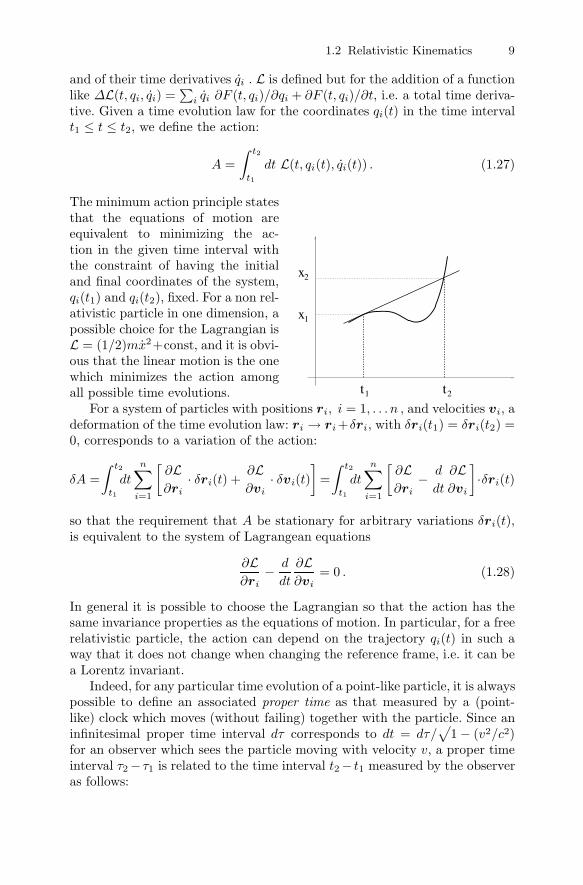
The minimum action principle statesthat the equations of motion areequivalent to minimizing the ac-tion in the given time interval withthe constraint of having the initialand final coordinates of the system,qi(t1) and qi(t2), fixed. For a non rel-ativistic particle in one dimension, apossible choice for the Lagrangian isL = (1/2)mx2+const, and it is obvi-ous that the linear motion is the onewhich minimizes the action amongall possible time evolutions. 1
x
x
t t2
1
2
For a system of particles with positions ri, i = 1, . . . n , and velocities vi, adeformation of the time evolution law: ri → ri +δri, with δri(t1) = δri(t2) =0, corresponds to a variation of the action:
δA =
∫ t2
t1
dt
n∑i=1
[∂L∂ri
· δri(t) +∂L∂vi
· δvi(t)
]=
∫ t2
t1
dt
n∑i=1
[∂L∂ri
− d
dt
∂L∂vi
]·δri(t)
so that the requirement that A be stationary for arbitrary variations δri(t),is equivalent to the system of Lagrangean equations
∂L∂ri
− d
dt
∂L∂vi
= 0 . (1.28)
In general it is possible to choose the Lagrangian so that the action has thesame invariance properties as the equations of motion. In particular, for a freerelativistic particle, the action can depend on the trajectory qi(t) in such away that it does not change when changing the reference frame, i.e. it can bea Lorentz invariant.
Indeed, for any particular time evolution of a point-like particle, it is alwayspossible to define an associated proper time as that measured by a (point-like) clock which moves (without failing) together with the particle. Since aninfinitesimal proper time interval dτ corresponds to dt = dτ/
√1− (v2/c2)
for an observer which sees the particle moving with velocity v, a proper timeinterval τ2− τ1 is related to the time interval t2− t1 measured by the observeras follows:
10 1 Introduction to Special Relativity
∫ t2
t1
dt
√1− v2(t)
c2=
∫ τ2
τ1
dτ = τ2 − τ1 . (1.29)
The integral on the left hand side does not depend on the reference frame ofthe observer, since in any case it must correspond to the time interval τ2 − τ1
measured by the clock at rest with the particle: the proper time τ of themoving system is therefore a Lorentz invariant by definition.
The action of a free relativistic particle is a time integral depending onthe evolution trajectory r = r(t) and, in order to be invariant under Lorentztransformations, it must necessarily be proportional to the proper time
A = k
∫ t2
t1
dt
√1− v2
c2, (1.30)
so that Lfree = k√
1− (v2/c2). For velocities much smaller than c, we canuse a Taylor expansion
Lfree = k
(1− 1
2
v2
c2− 1
8
v4
c4+ . . .
)(1.31)
which, compared with the Lagrangian of a non relativistic free particle, givesk = −mc2.
Let us now consider a scattering process involving n particles. The La-grangian of the system at the beginning and at the end of the process, i.e. faraway from when the interactions among the particles are not negligible, mustbe equal to the sum of the Lagrangians of the single particles, i.e.
L(t)||t|→∞ →n∑
i=1
Lfree,i = −n∑
i=1
mic2
√1− v2
i
c2, (1.32)
where L(t) is in general the complete Lagrangian describing also the interac-tion process and Lfree,i is the Lagrangian for the i-th free particle.
If no external forces are acting on the particles, L is invariant under trans-lations, i.e. it does not change if the positions of all particles are translated bythe same vector a: ri → ri + a. This invariance requirement can be writtenas:
∂L∂a
=
n∑i=1
∂L∂ri
= 0 . (1.33)
Combining this with the Lagrangean equations (1.28), we obtain the conser-
vation law:d
dt
n∑i=1
∂L∂vi
= 0 . (1.34)
That means that the sum of the vector quantities ∂L/∂vi does not changewith time, hence in particular:
1.2 Relativistic Kinematics 11
n∑i=1
∂Lfree,i
∂vi
|t→−∞ =n∑
i=1
∂Lfree,i
∂vi
|t→∞ . (1.35)
In the case of relativistic particles, taking into account the following identity:
∂
∂v
√1− v2
c2= − v
c2√
1− v2/c2(1.36)
and setting vi|t→−∞ = vi,I and vi|t→∞ = vi,F , equation (1.34) reads
n∑i=1
mivi,I√1− v2
i,I/c2=
n∑i=1
mivi,F√1− v2
i,F /c2. (1.37)
Invariance under translations is always related to the conservation of the totalmomentum of the system, hence we infer that mv/
√1− v2/c2 is the gener-
alization of momentum for a relativistic particle, as it is also clear by takingthe limit v/c→ 0.
Till now we have considered the case in which the final particles coincidewith the initial ones. However, in the relativistic case, particles can in generalchange their nature during the scattering process, melting together or split-ting, losing or gaining mass, so that the final set of particles is different fromthe initial one. It is possible, for instance, that the collision of two particlesleads to the production of new particles, or that a single particle spontaneouslydecays into two or more different particles. We are not interested at all, in thepresent context, in the specific dynamic laws regulating the interaction pro-cess; however we can say that, in absence of external forces, the invariance ofthe Lagrangian under spatial translation, expressed in (1.33), is valid anyway,together with the conservation law for the total momentum of the system. Ifwe refer in particular to the initial and final states, in which the system can bedescribed as composed by non-interacting free particles, the conservation lawimplies that the sum of the momenta of the initial particles be equal to thesum of the momenta of the final particles, so that (1.37) can be generalizedto
nI∑i=1
m(I)i vi,I√
1− v2i,I/c2
=
nF∑j=1
m(F )j vj,F√
1− v2j,F /c2
, (1.38)
where m(I)i and m
(F )j are the masses of the nI initial and of the nF final
particles respectively.Similarly, if the Lagrangian does not depend explicitly on time, it is pos-
sible, using again (1.28), to derive
d
dtL =
∑i
(vi · ∂L
∂vi
+ vi · ∂L∂ri
)
=∑
i
(vi · ∂L
∂vi
+ vi · d
dt
∂L∂vi
)=
d
dt
∑i
vi · ∂L∂vi
(1.39)

12 1 Introduction to Special Relativity
which is equivalent to the conservation law
d
dt
[∑i
vi · ∂L∂vi
− L]
= 0 . (1.40)
In the case of free relativistic particles, the conserved quantity in (1.40) is
∑i
(vi · mivi√
1− v2i /c2
+ mic2
√1− v2
i
c2
)=∑
i
mic2√
1− v2i /c2
. (1.41)
In the non relativistic limit mc2/√
1− v2/c2 � mc2 + 12mv2 apart from terms
proportional to v4, so that (1.41) becomes the conservation law for the sumof the non-relativistic kinetic energies of the particles (indeed, in the samelimit, Galilean invariance laws impose conservation of mass). We can thereforeconsider mc2/
√1− v2/c2 as the relativistic expression for the energy of a
free particle, as it should be clear from the fact that invariance under timetranslations is always related to the conservation of the total energy. Theanalogous of (1.38) is
nI∑i=1
m(I)i c2√
1− v2i,I/c2
=
nF∑j=1
m(F )j c2√
1− v2j,F /c2
. (1.42)
It is interesting to consider how the momentum components and the energyof a particle of mass m transform when going from one reference frame O toa new frame O′ moving with velocity v1, which is taken for simplicity to beparallel to the x axis. Let v be the modulus of the velocity of the particleand (vx, vy , vz) its components in O; in order to simplify the notation, let us
set β = v/c, β1 = v1/c, γ = 1/√
1− β2 and γ1 = 1/√
1− β21 , so that the
momentum components and the energy of the particle in O are
(px, py, pz) = (γmvx, γmvy, γmvz) , E = γmc2 . (1.43)
The modulus v′ of the velocity of the particle in O′ is easily found by using(1.19) (see Problem 1.7):
β′2 =v′2
c2= 1− 1
γ2γ21
1
(1− v1vx/c2)2, γ′ ≡ 1√
1− β′2= γγ1
(1− v1vx
c2
)
so that, using again (1.19):
p′x = γ′mv′x = γ1γm(1− v1vx
c2
) (vx − v1)
1− v1vx/c2= γ1
(px − v1
c
E
c
);
p′y/z = γ′mv′y/z = γ1γ(1− v1vx
c2
) mvy/z
γ1(1− v1vx/c2)= py/z ; (1.44)
1.2 Relativistic Kinematics 13
E′ = γ′mc2 = γ1γmc2(1− v1vx
c2
)= γ1
(E − v1
cpxc
).
Equations (1.44) show that the quantities (p, E/c) transform in the sameway as (x, ct), i.e. as the components of a quadrivector, so that the quan-tity |p|2 − E2/c2 does not change from one inertial reference frame to theother, the invariant quantity being directly linked to the mass of the par-ticle, |p|2 − E2/c2 = −m2c2. Moreover, given two different particles, wecan construct various invariant quantities from their momenta and ener-gies, among which p1 · p2 − E1E2/c2. The fact that momentum and en-ergy transform as a quadrivector can also be easily deduced by noticing that(p, E/c) = m(dx/dτ, c dt/dτ) and recalling that the proper time τ is a Lorentzinvariant quantity.
If we are dealing with a system of particles, we can also build up the totalmomentum P tot of the system, which is the sum of the single momenta, andthe total energy Etot, which is the sum of the single particle energies: sincequadrivectors transforms linearly, the quantity (P tot, Etot/c), being the sumof quadrivectors, transforms as a quadrivector as well; its invariant length islinked to a quantity which is called the invariant mass (Minv) of the system
|P tot|2 − E2tot/c2 ≡ −M2
inv c2 . (1.45)
It is often convenient to consider the center-of-mass frame for a system ofparticles, which is defined as the reference frame where the total momentumvanishes. It is easily verified, by using Lorentz transformations, that the centerof mass moves with a relative velocity
vcm =P tot
Etotc2 (1.46)
with respect to an inertial frame where P tot = 0. Notice that, according to(1.45) and (1.46), the center of mass frame is well defined only if the invariantmass of the system is different from zero.
On the basis of what we have deduced about the transformation propertiesof energy and momentum, it is important to notice that we can identify themas the components of a quadrivector only if the energy of a particle is definedas mc2/
√1− v2/c2, thus fixing the arbitrary constant usually appearing in
its definition. We can then assert that a particle at rest has energy equal tomc2. Since mass in general is not conserved3, it may happen that part of therest energy of a decaying particle gets transformed into the kinetic energies ofthe final particles, or that part of the kinetic energy of two or more particles
3 We mean by that the sum of the masses of the single particles. The invariant massof a system of particles defined in (1.45) is instead conserved, as a consequenceof the conservation of total momentum and energy.

14 1 Introduction to Special Relativity
involved in a diffusion process is transformed in the rest energy of the finalparticles. As an example, the energy which comes out of a nuclear fissionprocess derives from the excess in mass of the initial nucleus with respect tothe masses of the products of fission. Everybody knows the relevance that thissimple remark has acquired in the recent past.
A particular discussion is required for particles of vanishing mass, like thephoton. While, according to (1.37) and (1.41), such particles seem to havevanishing momentum and energy, a more careful look shows that the limitm → 0 can be taken at constant momentum p if at the same time the speedof the particle tends to c according to v = c (1 + m2p2/c2)−1/2. In the samelimit E → pc, in agreement with p2 − E2/c2 = −m2c2.
Our considerations on conservation and transformation properties of en-ergy and momentum permit to fix in a quite simple way the kinematic con-straints related to a diffusion process: let us illustrate this point with anexample.
In relativistic diffusion processes it is possible to produce new particlesstarting from particles which are commonly found in Nature. The collision oftwo hydrogen nuclei (protons), which have a mass m � 1.67 10−27 Kg, cangenerate the particle π, which has a mass μ � 2.4 10−28 Kg. Technically, someprotons are accelerated in the reference frame of the laboratory, till one obtainsa beam of momentum P , which is then directed against hydrogen at rest. Thatleads to proton–proton collisions from which, apart from the already existingprotons, also the π particles emerge (it is possible to describe schematicallythe reaction as p + p → p + p + π). A natural question regards the minimummomentum or energy of the beam particles needed to produce the reaction: inorder to get an answer, it is convenient to consider this problem as seen fromthe center of mass frame, in which the two particles have opposite momenta,which we suppose to be parallel, or anti-parallel, to the x axis: P1 = −P2,and equal energies E1 =
√P 2
1 c2 + m2c4 = E2. In this reference frame thetotal momentum vanishes and the total energy is E = 2E1. Conservation ofmomentum and energy constrains the sum of the three final particle momentato vanish, and the sum of their energy to be equal to E. The required energy isminimal if all final particles are produced at rest, the kinematical constrainton the total momentum being automatically satisfied in that case (this isthe advantage of doing computations in the center of mass frame). We canthen conclude that the minimum value of E in the center of mass is Emin =(2m + μ)c2. However that is not exactly the answer to our question: we haveto find the value of the energy of the beam protons corresponding to a totalenergy in the center of mass equal to Emin. That can be done by noticingthat in the center of mass both colliding protons have energy Emin/2, so thatwe can compute the relative velocity βc between the center of mass and thelaboratory as that corresponding to a Lorentz transformation leading from aproton at rest to a proton with energy Emin/2, i.e. solving the equation
1.2 Relativistic Kinematics 15
1√1− β2
=Emin
2mc2=
2m + μ
2m.
While, as said above, the total momentum of the system vanishes in the centerof mass frame and the total energy equals Emin, in the laboratory the totalmomentum is obtained by a Lorentz transformation as
PL =β√
1− β2
Emin
c=
√1
1− β2− 1
Emin
c= (2m + μ)c
√(2m + μ)2
4m2− 1
=2m + μ
2mc√
4mμ + μ2 .
This is also the answer to our question, since in the laboratory all momentumis carried by the proton of the beam.
An alternative way to obtain the same result, without making explicit useof Lorentz transformations, is to notice that, if EL is the total energy in thelaboratory, P 2
L − E2L/c2 is an invariant quantity, which is therefore equal to
the same quantity computed in the center of mass, so that
P 2L −
E2L
c2= −(2m + μ)2c2 .
Writing EL as the sum of the energy of the proton in the beam, which is√P 2
Lc2 + m2c4, and of that of the proton at rest, which is mc2, we have thefollowing equation for PL:
P 2L −
1
c2
[√P 2
Lc2 + m2c4 + mc2
]2
= −(2m + μ)2c2 ,
which finally leads to the same result obtained above.
Suggestions for Supplementary Readings
• C. Kittel, W. D. Knight, M. A. Ruderman: Mechanics - Berkeley Physics Course,volume 1 (Mcgraw-Hill Book Company, New York 1965)
• L. D. Landau, E. M. Lifshitz: The Classical Theory of Fields - Course of theo-
retical physics, volume 2 (Pergamon Press, London 1959)• J. D. Jackson: Classical Electrodynamics, 3d edn (John Wiley, New York 1998)• W. K. H. Panowsky, M. Phillips: Classical Electricity and Magnetism, 2nd edn
(Addison-Wesley Publishing Company Inc., Reading 2005)
16 1 Introduction to Special Relativity
Problems
1.1. A spaceship of length L0 = 150 m is moving with respect to a spacestation with a speed v = 2 108 m/s. What is the length L of the spaceship asmeasured by the space station?
Answer: L = L0
√1− v2/c2 � 112 m .
1.2. How many years does it take for an atomic clock (with a precision ofone part over 1015), which is placed at rest on Earth, to lose one second withrespect to an identical clock placed on the Sun? (Hint: apply Lorentz trans-formations as if both reference frames were inertial, with a relative velocityv � 3 104 m/s � 10−4 c).
Answer: Setting Δt = 1 s we have T = Δt/(1−
√1− v2/c2
)� 2Δt c2/v2 �
6.34 years .
1.3. An observer casts a laser pulse of frequency ν = 1015 Hz against a mir-ror, which is moving with a speed v = 5 107 m/s opposite to the direction ofthe pulse, and whose surface is orthogonal to it. The observer then measuresthe frequency ν′ of the pulse coming back after being reflected by the mirror.What is the value of ν′?
Answer: Since reflection leaves the frequency unchanged only in the rest frame
of the mirror, two different longitudinal Doppler effects have to be taken into ac-
count, that of the original pulse with respect to the mirror and that the reflected
pulse with respect to the observer, therefore ν′ = ν (1+v/c)/(1−v/c) = 1.4 1015 Hz .
1.4. Fizeau’s Experiment
In the experiment described in the figure, a light beam of frequency ν =1015 Hz, produced by the source S, is split into two distinct beams whichgo along two different paths belonging to a rectangle of sides L1 = 10 mand L2 = 5 m. They recombine, producing interference in the observationpoint O, as illustrated in the figure. The rectangular path is contained in atube T filled with a liquid having refraction index n = 2, so that the speedof light in that liquid is vc � 1.5 108 m/s. If the liquid is moving counter-clockwise around the tube with a velocity 0.3 m/s, the speed of the lightbeams along the two different paths changes, together with their wavelength,which is constrained by the equation vc = λν (the frequency ν instead doesnot change and is equal to that of the original beam). For that reason thetwo beams recombine in O with a phase difference Δφ, which is different fromzero (the phase accumulated by each beam is given by 2π times the number ofwavelengths contained in the total path). What is the value of Δφ? Comparethe result with what would have been obtained using Galilean transformationlaws.

Problems 17
. . . . . . . . . . . . . . . . . . . . . . . . . . . . . .......... . . . . . . . . . . . . . . . . . . . . . . . . . . . . .
.
..
..
..
.
�� �
� �
S
O
T
Answer: Calling L = L1 +L2 = 15 m the total path length inside the tube for eachbeam, and using Einstein laws for adding velocities, one finds
Δφ = 4πνLvn2 − 1
c2 − n2v2� 4πνLv(n2 − 1)/c2 � 1.89 rad .
Instead, Galilean laws would lead to
Δφ = 4πνLvn2
c2 − n2v2,
a result which does not make sense, since it is different from zero also when the tube
is empty: in that case, indeed, Galilean laws would imply that the tube is still filled
with a “rotating ether”.
1.5. A flux of particles, each carrying an electric charge q = 1.6 10−19 C, ismoving along the x axis with a constant velocity v = 0.9 c. If the total carriedcurrent is I = 10−9 A, what is the linear density of particles, as measured inthe reference frame at rest with them?
Answer: If d0 is the distance among particles in their rest frame, the distancemeasured in the laboratory appears contracted and equal to d =
√1− v2/c2 d0.
The electric current is given by I = d−1vq, hence the particle density in the restframe is
d−10 =
√1− v2/c2
I
vq� 10.1 particles/m .
1.6. A particle is moving with a velocity c/2 along the positive direction ofthe line y = x. What are the components of the velocity of the particle for anobserver moving with a speed V = 0.99 c along the x axis?
Answer: We have vx = vy = c/(2√
2) in the original system. After applying rela-tivistic laws for the addition of velocities we find
v′x =
vx − V
1− vxV/c2� −0.979c ; v′
y =√
1− V 2/c2vy
1− vxV/c2� 0.0767c .
1.7. A particle is moving with a speed of modulus v and components (vx, vy, vz).What is the modulus v′ of the velocity for an observer moving with a speedw along the x axis? Comment the result as v and/or w approach c.
Answer: Applying the relativistic laws for the addition of velocities we find
18 1 Introduction to Special Relativity
v′2 = v′2x + v′2
y + v′2z =
(vx − w)2 + (1− w2/c2)(v2z + v2
y)
(1− vxw/c2)2
and after some simple algebra
v′2 = c2
(1− (1− v2/c2)(1− w2/c2)
(1− vxw/c2)2
).
It is interesting to notice that as v and/or w approach c, also v′ approaches c (from
below): that verifies that a body moving with v = c moves with the same velocity
in every reference frame (invariance of the speed of light).
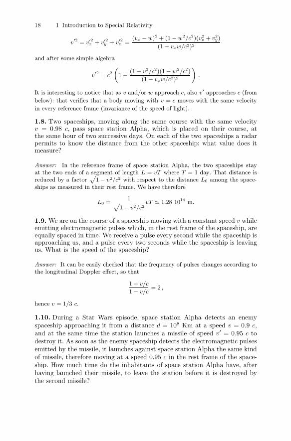
1.8. Two spaceships, moving along the same course with the same velocityv = 0.98 c, pass space station Alpha, which is placed on their course, atthe same hour of two successive days. On each of the two spaceships a radarpermits to know the distance from the other spaceship: what value does itmeasure?
Answer: In the reference frame of space station Alpha, the two spaceships stayat the two ends of a segment of length L = vT where T = 1 day. That distance isreduced by a factor
√1− v2/c2 with respect to the distance L0 among the space-
ships as measured in their rest frame. We have therefore
L0 =1√
1− v2/c2vT � 1.28 1014 m.
1.9. We are on the course of a spaceship moving with a constant speed v whileemitting electromagnetic pulses which, in the rest frame of the spaceship, areequally spaced in time. We receive a pulse every second while the spaceship isapproaching us, and a pulse every two seconds while the spaceship is leavingus. What is the speed of the spaceship?
Answer: It can be easily checked that the frequency of pulses changes according tothe longitudinal Doppler effect, so that
1 + v/c
1− v/c= 2 ,
hence v = 1/3 c.
1.10. During a Star Wars episode, space station Alpha detects an enemyspaceship approaching it from a distance d = 108 Km at a speed v = 0.9 c,and at the same time the station launches a missile of speed v′ = 0.95 c todestroy it. As soon as the enemy spaceship detects the electromagnetic pulsesemitted by the missile, it launches against space station Alpha the same kindof missile, therefore moving at a speed 0.95 c in the rest frame of the space-ship. How much time do the inhabitants of space station Alpha have, afterhaving launched their missile, to leave the station before it is destroyed bythe second missile?

Problems 19
Answer: Let us make computations in the reference frame of space station Al-
pha. Setting to zero the launching time of the first missile, the enemy spaceship
detects it and launches the second missile at time t1 = d/(v + c) and when it is at
a distance x1 = cd/(v + c) from the space station. The second missile approaches
Alpha with a velocity V = (v + v′)/(1 + vv′/c2) � 0.9973 c, therefore it hits the
space station at time t2 = t1 + x1/V � 352 s.
1.11. A particle moves in one dimension with an acceleration which is con-stant and equal to a in the reference frame instantaneously at rest with it.Determine, for t > 0, the trajectory x(t) of the particle in the reference frameof the laboratory, where it is placed at rest in x = 0 at time t = 0.
Answer: Let us call τ the proper time of the particle, synchronized so that τ = 0when t = 0. The relation between proper and laboratory time is given by
dτ =√
1− v2(t)/c2 dt
where v(t) = dx/dt is the particle velocity in the laboratory. Let us also introducethe quadrivelocity (dx/dτ, d(ct)/dτ ), which transforms as a quadrivector since dτ isa Lorentz invariant. We are interested in particular in its spatial component in onedimension, u ≡ dx/dτ , which is related to v by the following relations
u =v√
1− v2/c2, v =
u√1 + u2/c2
,
√1 +
u2
c2
√1− v2
c2= 1 .
To derive the equation of motion, let us notice that, in the frame instantaneouslyat rest with the particle, the velocity goes from 0 to adτ in the interval dτ , sothat v changes into (v + adτ )/(1 + vadτ/c2) in the same interval, meaning thatdv/dτ = a(1− v2/c2). Using previous equations, it is easy to derive
du
dt=
du
dv
dv
dτ
dτ
dt= a
which can immediately be integrated, with the initial condition u(0) = v(0) = 0, asu(t) = at. Using the relation between u and v we have
v(t) =at√
1 + a2t2/c2.
That gives the variation of velocity, as observed in the laboratory, for a uniformlyaccelerated motion: for t � c/a one recovers the non-relativistic result, while fort � c/a the velocity reaches asymptotically that of light. The dependence of v on tcan be finally integrated, using the initial condition x(0) = 0, giving
x(t) =c2
a
(√1 +
a2t2
c2− 1
).
1.12. Spaceship A is moving with respect to space station S with a velocity2.7 108 m/s. Both A and S are placed in the origin of their respective referenceframes, which are oriented so that the relative velocity of A is directed along
20 1 Introduction to Special Relativity
the positive direction of both x axes; A and S meet at time tA = tS = 0.Space station S detects an event, corresponding to the emission of luminouspulse, in xS = 3 1013 m at time tS = 0. An analogous but distinct event isdetected by spaceship A, with coordinates xA = 1.3 1014 m , tA = 2.3 103 s. Isit possible that the two events have been produced by the same moving body?
Answer: The two events may have been produced by the same moving body only
if they have a time-like distance, otherwise the unknown body would go faster
than light. After obtaining the coordinates of the two events in the same ref-
erence frame, one obtains, e.g. in the spaceship frame, Δx � 6.09 1013 m and
cΔt � 6.27 1013 m > Δx: the two events may indeed have been produced by the
same body moving at a speed Δx/Δt � 0.97 c.
1.13. We are moving towards a mirror with a velocity v orthogonal to itssurface. We send an electromagnetic pulse of frequency ν = 109 Hz towardsthe mirror, along the same direction of our motion. After 2 seconds we receivea reflected pulse of frequency ν′ = 1.32 109 Hz. How many seconds are leftbefore our impact with the mirror?
Answer: We can deduce our velocity with respect to the mirror by using the double
longitudinal Doppler effect: v = βc with (1 + β)/(1− β) = 1.32, hence v = 0.138 c.
One second after we emit our pulse, the mirror is placed at one light-second from
us, therefore the impact will take place after ΔT = 1/0.138 s � 7.25 s, that means
6.25 s after we receive the reflected pulse.
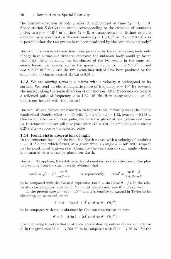
1.14. Relativistic aberration of lightIn the reference frame of the Sun, the Earth moves with a velocity of modulusv = 10−4 c and which forms, at a given time, an angle θ = 60◦ with respectto the position of a given star. Compute the variation of such angle when itis measured by a telescope placed on Earth.
Answer: By applying the relativistic transformation laws for velocities to the pho-tons coming from the star, it easily obtained that
tan θ′ =√
1− β2sin θ
cos θ + βor equivalently cos θ′ =
cos θ + β
1 + β cos θ
to be compared with the classical expression tan θ′ = sin θ/(cos θ + β). In the rela-tivistic case all angles, apart from θ = π, get transformed into θ′ = 0 as β → 1.
In the present case β = v/c = 10−4 and it is sensible to expand in Taylor seriesobtaining, up to second order:
θ′ = θ − β sin θ + β2 sin θ cos θ + O(β3)
to be compared with result obtained by Galilean transformation laws:
θ′ = θ − β sin θ + 2β2 sin θ cos θ + O(β3) .
It is interesting to notice that relativistic effects show up only at the second order in
β. In the given case δθ = −17.86216′′ to be compared with δθ = −17.86127′′ for the

Problems 21
classical computation. Relativistic effects are tiny in this case and not appreciable
by a usual optical telescope; an astronomical interferometer, which is able to reach
resolutions of the order of few micro-arcseconds at radio wavelengths, should be used
instead.
1.15. A particle μ (muon), of mass m = 1.89 10−28 Kg and carrying the sameelectric charge as the electron, has a mean life time τ = 2.2 10−6 s when itis at rest. The particle is accelerated instantaneously through a potential gapΔV = 108 V. What is the expected life time t of the particle, in the labora-tory, after the acceleration? What is the expected distance D traveled by theparticle before decaying?
Answer:
t = τ(mc2 + eΔV )
mc2� 4.28 10−6 s
D =
√(eΔV )2 + 2emc2ΔV
mc2cτ = 1.1 103 m .
Notice that the average traveled distance D is larger than what expected in absence
of time dilatation, which is limited to cτ due to the finiteness of the speed of light.
The increase in the traveled distance for relativistic unstable particles is one of the
best practical proofs of time dilatation, think e.g. of the muons created when cosmic
rays collide with the upper regions of the atmosphere: a large fraction of them reaches
Earth’s surface and that is possible only because their life times appear dilated in
Earth’s frame.
1.16. The energy of a particle is equal to 2.5 10−12 J, its momentum is7.9 10−21 N s. What are its mass m and velocity v?
Answer: m =√
E2 − c2p2/c2 � 8.9 10−30 Kg , v = pc2/E � 2.84 108m/s.
1.17. A spaceship with an initial mass M = 103 Kg is boosted by a photonicengine: a light beam is emitted opposite to the direction of motion, with apower W = 1015 W, as measured in the spaceship rest frame. What is thederivative of the spaceship rest mass with respect to its proper time? Whatis the spaceship acceleration a in the frame instantaneously at rest with it?
Answer: The engine power must be subtracted from the spaceship energy, which isMc2 in its rest frame, hence dM/dt = −W/c2 � 1.1 10−2 Kg/s. Since the particlesemitted by the engine are photons, they carry a momentum equal to 1/c times theirenergy, hence
a(τ ) =W
c(M −Wτ/c2).
1.18. A spaceship with an initial mass M = 3 104 Kg is boosted by a pho-tonic engine of constant power, as measured in the spaceship rest frame, equalto W = 1013 W. If the spaceship moves along the positive x direction andleaves the space station at τ = 0, compute its velocity with respect to thestation reference frame (which is assumed to be inertial) as a function of the

22 1 Introduction to Special Relativity
spaceship proper time.
Answer: According to the solution of previous Problem 1.17, the spaceship ac-celeration a in the frame instantaneously at rest with it is
a(τ ) =W
cM(τ )=
W
c(M − τW/c2)=
a0
1− ατ, a0 � 1.1 m/s2 , α � 3.7 10−9 s−1 .
Recalling from the solution of Problem 1.11 that
v =u√
1 + u2
c2
,du
dτ= a(τ )
√1 +
u2
c2,
where u is the x-component of the quadrivelocity, we can easily integrate last equa-tion
du√1 + u2
c2
=a0dτ
1− ατ
obtainingu
c= sinh
(− a0
αcln(1− ατ )
).
Expressing v/c as a function of u/c we finally get
v
c= tanh
(− a0
αcln(1− ατ )
)=
1− (1− ατ )2a0/αc
1 + (1− ατ )2a0/αc.
1.19. A spaceprobe of mass M = 10 Kg is boosted by a laser beam of fre-quency ν = 1015 Hz and power W = 1012 W, which is directed from Earthagainst an ideal reflecting mirror (i.e. reflecting all incoming photons) placed inthe back of the probe. Assuming that the probe is initially at rest with respectto Earth, and that the laser beam is always parallel to the spaceprobe velocityand orthogonal to the mirror, determine the evolution of the spaceprobe po-sition in the Earth frame and compute the total time Δt for which the lasermust be kept switched on in order that the spaceprobe reaches a velocityv = 0.5 c.
Answer: In the reference frame of the spaceship, every photon gets reflected fromthe mirror with a negligible change in frequency (Δλ′/λ′ ∼ hν′/(Mc2) < 10−37, seeProblem 1.29), hence it transfers a momentum 2hν′/c to the spaceprobe, where ν′
is the photon frequency in the spaceprobe frame. The acceleration of the probe inits proper frame is therefore
a′ =2hν′
Mc
dN ′γ
dt′=
2W ′
Mc
where W ′ is the power of the beam measured in the proper frame, which is givenby the photon energy, hν′, times the rate at which photons arrive, i.e. the numberof photons hitting the mirror per unit time, dN ′
γ/dt′. The above result is twice aslarge as that obtained if the light beam is emitted directly by the spaceprobe, as inProblem 1.17, since in this case each reflected photon transfers twice its momentum.

Problems 23
Both ν′ and the rate of arriving photons are frequencies, hence they get trans-formed by Doppler effect and we can write
W ′ = hν′ dN ′γ
dt′=
√1− β
1 + βhν
√1− β
1 + β
dNγ
dt=
1− β
1 + βW
which gives us the transformation law for the beam power. From the acceleration inthe proper frame, a′ = 2W (1−β)/[(1 + β)Mc], one obtains the derivative of β withrespect to the proper time τ (see Problem 1.11)
dβ
dτ=
dv
cdτ=
a′
c
(1− v2
c2
)= α(1− β)2
where we have set α = 2W/(Mc2). Last equation, after integration with the initialcondition β(0) = 0, leads to ατ = β/(1− β), i.e.
β(τ ) =ατ
1 + ατ.
Regarding the position of the probe, we have
dx = cβdt = cβdτ√1− β2
=ατ√
1 + 2ατdτ
which gives, after integration and using x(0) = 0
x =c
3α
((ατ − 1)
√2ατ + 1 + 1
).
Setting β = 0.5 we obtain τ = α−1 = Mc2/(2W ) = 9 105 s. The corresponding timein the Earth frame can be obtained by integrating the relation
dt =dτ√1− β2
=1 + ατ√1 + 2ατ
dτ
yielding
t =1
3α
((ατ + 2)
√2ατ + 1− 2
).
In order to compute the total time Δt that the laser must be kept switched on, wehave to consider that a photon reaching the spaceprobe at time t has left Earth ata time t− x(t)/c, where x is the probe position, hence the emission time is
tem = t− x/c =1
α
(√2ατ + 1− 1
).
Setting ατ = 1, we obtain Δt = (√
3− 1)/α � 6.59 105 s .
1.20. An electron–proton collision can give rise to a fusion process in whichall available energy is transferred to a neutron. As a matter of fact, there is aneutrino emitted whose energy and momentum in the present situation can beneglected. The proton rest energy is 0.938 109 eV, while those of the neutronand of the electron are respectively 0.940 109 eV and 5 105 eV. What is thevelocity of the electron which, knocking into a proton at rest, may give riseto the process described above?

24 1 Introduction to Special Relativity
Answer: Notice that we are not looking for a minimum electron energy: since,neglecting the final neutrino, the final state is a single particle state, its invariantmass is fixed and equal to the neutron mass. That must be equal to the invariantmass of the initial system of two particles, leaving no degrees of freedom on the pos-sible values of the electron energy: only for one particular value ve of the electronvelocity the reaction can take place.
A rough estimate of ve can be obtained by considering that the electron energy
must be equal to the rest energy difference (mn−mp) c2 = (0.940−0.938) 109 eV plus
the kinetic energy of the final neutron. Therefore the electron is surely relativistic and
(mn−mp)c is a reasonable estimate of its momentum: it coincides with the neutron
momentum which is instead non-relativistic ((mn − mp)c � mnc). The kinetic
energy of the neutron is thus roughly (mn −mp)2c2/(2mn), hence negligible with
respect to (0.940−0.938) 109 eV. The total electron energy is therefore, within a good
approximation, Ee � 2 106 eV, and its velocity is ve = c√
1−m2e/E2
e � 2.9 108 m/s.
The exact result is obtained by writing Ee = (m2n−m2
p−m2e)c
2/(2mp), which differs
by less than 0.1 % from the approximate result.
1.21. A system made up of an electron and a positron, which is an exact copyof the electron but with opposite charge (i.e. its antiparticle), annihilates,while both particles are at rest, into two photons. The mass of the electron isme � 0.9 10−30 Kg: what is the wavelength of each outgoing photon? Explainwhy the same system cannot decay into a single photon.
Answer: The two photons carry momenta of modulus mc which are opposite to
each other in order to conserve total momentum: their common wavelength is there-
fore, as we shall see in next Chapter, λ = h/(mec) � 2.4 10−12 m. A single photon
should carry zero momentum since the initial system is at rest, but then energy
could not be conserved; more in general the initial invariant mass of the system,
which is 2me, cannot fit the invariant mass of a single photon, which is always zero.
1.22. A piece of copper of mass M = 1 g, is heated from 0◦C up to 100◦C.What is the mass variation ΔM if the copper specific heat is CCu = 0.4 J/g◦C?
Answer: The piece of copper is actually a system of interacting particles whose
mass is defined as the invariant mass of the system. That is proportional to
the total energy if the system is globally at rest, see equation (1.45). Therefore
ΔM = CCu ΔT/c2 � 4.45 10−16 Kg .
1.23. Consider a system made up of two point-like particles of equal massm = 10−20 Kg, bound together by a rigid massless rod of length L = 2 10−4 m.The center of mass of the system lies in the origin of the inertial frame O, inthe same frame the rod rotates in the x − y plane with an angular velocityω = 3 1010 s−1. A second inertial reference frame O′ moves with respect to Owith velocity v = 4c/5 parallel to the x axis. Compute the sum of the kineticenergies of the particles at the same time in the frame O′, disregarding cor-rection of order ω3.

Problems 25
Answer: There are two independent ways of computing the sum of the kinetic
energies of the particles. The first way, which is the simplest one, is based on
the assumption that the kinetic energy of the system coincides with the sum
of the kinetic energies of the particles, hence one can compute the total en-
ergy of the system in the reference O, which, in the chosen approximation, is:
Et = m (2c2 + ω2L2/4). In O′ the total energy is computed by a Lorentz trans-
formation E′t = Et/
√1− v2/c2 = (5/3)m (2c2 + ω2L2/4), hence the sum of
the kinetic energies is E′t − 2mc2 = 4/3mc2 + 5mω2L2/12. Numerically one has
12 10−4(1 + 1.25 10−4) J. Alternatively, we can compute the velocities of both
particles in a situation corresponding to equal time in O′. The simplest such situ-
ation is when the rod is parallel to the y axis and the particles move with velocity
v± = ±ωL/2 parallel to the x axis. Using Einstein formula one finds in O′ the
velocities v′± = c(4/5 ± ωL/(2c))/(1 ± 2ωL/(5c)) and hence the kinetic energies
E′± = mc2(1/
√1− (v′
±/c)2 − 1) = mc2((5± 2ωL/c)/(3
√1− (ωL/(2c))2)− 1
). It
is apparent that the sum E′+ + E′
− gives the known result up to corrections of order
(ωL/c)4.
1.24. A photon of energy E knocks into an electron at rest producing a finalstate composed of an electron–positron pair plus the initial electron: all threefinal particles have the same momentum. What is the value of E and thecommon momentum p of the final particles?
Answer: E = 4 mc2 � 3.3 10−13 J , p = E/3c = 4/3 mc � 3.6 10−22 N/m .
1.25. A particle of mass M = 10−27 Kg decays, while at rest, into a particleof mass m = 4 10−28 Kg plus a photon. What is the energy E of the photon?
Answer: The two outgoing particles must have opposite momenta with an equalmodulus p to conserve total momentum. Energy conservation is then written asMc2 =
√m2c4 + p2c2 + pc, so that
E = pc =M2 −m2
2Mc2 = 0.42 Mc2 � 3.78 10−11 J � 2.36 108 eV .
1.26. A particle of mass M = 1 GeV/c2 and energy E = 10 GeV decays intotwo particles of equal mass m = 490 MeV. What is the maximum angle thateach of the two outgoing particles may form, in the laboratory, with the tra-jectory of the initial particle?
Answer: Let x be the direction of motion of the initial particle, and x–y the decayplane: this is defined as the plane containing both the initial particle momentumand the two final momenta, which are indeed constrained to lie in the same planeby total momentum conservation. Let us consider one of the two outgoing particles:in the center of mass frame it has energy ε = Mc2/2 = 0.5 GeV and a momentumpx = p cos θ, py = p sin θ, with θ being the decay angle in the center of mass frameand

26 1 Introduction to Special Relativity
p = c
√M2
4−m2 � 0.1 GeV
c.
The momentum components in the laboratory are obtained by Lorentz transfor-mations with parameters γ = (
√1− v2/c2)−1 = E/(Mc2) = 10 and β = v/c =√
1− 1/γ2 � 0.995,p′
y = py = p sin θ
p′x = γ(p cos θ + βε) .
It can be easily verified that, while in the center of mass frame the possible momen-tum components lie on a circle of radius p centered in the origin, in the laboratoryp′
x and p′y lie on an ellipse of axes γp and p, centered in (γβε, 0). If θ′ is the angle
formed in the laboratory with respect to the initial particle trajectory and definingα ≡ βε/p � 5, we can write
tan θ′ =p′
y
p′x
=1
γ
sin θ
cos θ + α.
If α > 1 the denominator is always positive, tan θ′ is limited and |θ′| < π/2, i.e.the particle is always forward emitted, in the laboratory, with a maximum possibleangle which can be computed by solving d tan θ′/dθ = 0; that can also be appreciatedpictorially by noticing that, if α > 1, the ellipse containing the possible momentumcomponents does not contain the origin. Finally one finds
θ′max = tan−1
(1
γ
1√α2 − 1
)� 0.02 rad .
1.27. A particle of mass M = 10−27 Kg, which is moving in the labo-ratory with a speed v = 0.99 c, decays into two particles of equal massm = 3 10−28 Kg. What is the possible range of energies (in GeV) whichcan be detected in the laboratory for each of the outgoing particles?
Answer: In the center of mass frame the outgoing particles have equal energyand modulus of the momentum completely fixed by the kinematic constraints:E = Mc2/2 and P = c
√M2/4−m2. The only free variable is the decaying angle
θ, measured with respect to the initial particle trajectory, which however results ina variable energy E′ in the laboratory frame. Indeed by Lorentz transformationsE′ = γ(E + vP cos θ), with γ = (1− v2/c2)−1/2, hence
E′max/min = γ
(Mc2
2± v
cPc
)⇒ E′
max � 3.56 GeV , E′min � 0.41 GeV .
1.28. A particle of rest energy Mc2 = 109 eV, which is moving in the labo-ratory with momentum p = 5 10−18 N s, decays into two particles of equalmass m = 2 10−28 Kg. In the center of mass frame the decay direction isorthogonal to the trajectory of the initial particle. What is the angle betweenthe trajectories of the outgoing particles in the laboratory?
Answer: Let x be the direction of the initial particle and y the decay direction
in the center of mass frame, y ⊥ x. For the process described in the text, x is a

Problems 27
symmetry axis, hence the outgoing particles will form the same angle θ also in the
laboratory. For one of the two particles we can write px = p/2 by momentum conser-
vation in the laboratory, and py = c√
M2/4−m2 by energy conservation. Finally,
the angle between the two particles is 2θ = 2 atan(py/px) � 0.207 rad .
1.29. Compton EffectA photon of wavelength λ knocks into an electron at rest. After the elasticcollision, the photon moves in a direction forming an angle θ with respect toits original trajectory. What is the change Δλ ≡ λ′ − λ of its wavelength as afunction of θ?
Answer: Let q and q′ be respectively the initial and final momentum of the photon,and p the final momentum of the electron. As we shall discuss in next Chapter, thephoton momentum is related to its wavelength by the relation q ≡ |q| = h/λ, whereh is Planck’s constant. Total momentum conservation implies that q, q′ and p mustlie in the same plane, which we choose to be the x−y plane, with the x-axis parallelto the photon initial trajectory. Momentum and energy conservation lead to:
px = q − q′ cos θ ,
py = q′ sin θ ,
qc + mec2 − q′c =
√mec4 + p2
xc2 + p2yc2 .
Substituting the first two equations into the third and squaring both sides of thelast we easily arrive, after some trivial simplifications, to me(q− q′) = qq′(1− cos θ),which can be given in terms of wavelengths as follows
Δλ ≡ λ′ − λ =h
mec(1− cos θ) ;
Δλ
λ=
hν
mec2(1− cos θ) .
The difference is always positive, since part of the photon energy, depending on the
diffusion angle θ, is always transferred to the electron. This phenomenon, known as
Compton effect, is not predicted by the classical theory of electromagnetic waves and
is an experimental proof of the corpuscular nature of radiation. Notice that, while
the angular distribution of outgoing photons can only be predicted on the basis of
the quantum relativistic theory, i.e. Quantum Electrodynamics, the dependence of
Δλ on θ that we have found is only based on relativistic kinematics and can be
used to get an experimental determination of h. The coefficient h/(mec) is known
as Compton wavelength, which for the electron is of the order of 10−12 m, so that
the effect is not detectable (Δλ/λ � 0) for visible light.
1.30. A spinning top, which can be described as a rigid disk of mass M =10−1 Kg, radius R = 5 10−2 m and uniform density, starts rotating with an-gular velocity Ω = 103 rad/s. What is the energy variation of the spinningtop due to rotation, as seen from a reference frame moving with a relativespeed v = 0.9 c with respect to it?
Answer: The speed of the particles composing the spinning top is surely non-relativistic in their frame, since it is limited by ΩR = 50 m/s � 1.67 10−7 c. Inthat frame the total energy is therefore, apart from corrections of order (ΩR/c)2,

28 1 Introduction to Special Relativity
Etot = Mc2 + IΩ2/2, where I is the moment of inertia, I = MR2/2. Lorentz trans-formations yield in the moving frame
E′tot =
1√1− v2/c2
Etot =1√
1− v2/c2
(Mc2 +
1
2IΩ2
),
to be compared with energy observed in absence of rotation, Mc2/√
1− v2/c2.
Therefore, the energy variation due to rotation in the moving frame is ΔE′ =
IΩ2/(2√
1− v2/c2) � 143 J .
1.31. A photon with energy E1 = 104 eV is moving along the positive x di-rection; a second photon with energy E2 = 2 E1 is moving along the positivey direction. What is the velocity vcm of their center of mass frame?
Answer: Recalling equation (1.46), it is easily found that vxcm = 1/3 c, vy
cm = 2/3 c
and |vcm| =√
5/3 c.
1.32. A particle of mass M decays, while at rest, into three particles of equalmass m. What is the maximum and minimum possible energy for each of theoutgoing particles?
Answer: Let E1, E2, E3 and p1, p2, p3 be respectively the energies and the mo-menta of the three outgoing particles. We have to find, for instance, the maximumand minimum value of E1 which are compatible with the constraints p1+p2+p3 = 0and E1 + E2 + E3 = M c2. The minimum value is realized when the particle is pro-duced at rest, E1min = m c2, implying that the other two particles move with equaland opposite momenta. Finding the maximum value requires some more algebra.From E2
1 = m2 c4 + p21 c2 and momentum conservation we obtain
E21 = m2 c4 + |p2 + p3|2 c2 = m2 c4 + (E2 + E3)
2 − μ2 c4
where μ is the invariant mass of particles 2 and 3, μ2 c4 = (E2 +E3)2−|p2 +p3|2 c2.
Applying energy conservation, E2 + E3 = (M c2 − E1), last equation leads to
E1 =1
2M c2
(m2 c4 + M2 c4 − μ2 c4
).
We have written E1 as a function of μ2: E1max corresponds to the minimum possible
value for the invariant mass of the two remaining particles. On the other hand it
can be easily checked that, for a system made up of two or more massive particles,
the minimum possible value of the invariant mass is equal to the sum of the masses
and is attained when the particles are at rest in their center of mass frame, meaning
that the particles move with equal velocities in any other reference frame. Therefore
μmin = 2m and E1max = (M2 − 3m2) c2/(2M): this value is obtained in particular
for p2 = p3.
1.33. A particle at rest, whose mass is M = 750 MeV/c2, decays into a photonand a second, lighter, particle of mass m = 135 MeV/c2. Subsequently thelighter particle decays into two further photons. Considering all the possible

Problems 29
decay angles of the second particle, compute the maximum and the minimumvalues of the possible energies of the three final photons.
One can ask the same question in the case of a direct decay of the firstparticle into three photons whose energies are constrained only by energy-momentum conservation. Which are the maximum and minimum energies ofthe final photons in the direct decay?
Answer: This problem is analogous to Problem 1.32. We first consider the di-rect decay. If Ei with i = 1, 2 are the energies of two, arbitrarily chosen, fi-nal photons, pi = Ei/c are their momenta. If θ is the angle between these mo-menta, on account of momentum conservation, we can compute the momentumof the third photon as the length of the third side of a triangle whose othersides have lengths p1 and p2 and form an angle π − θ. Therefore energy con-servation gives:
√E2
1 + E22 + 2E1E2 cos θ + E1 + E2 = Mc2 from which we get:
M2c4 − 2Mc2(E1 + E2) = −2E1E2(1 − cos θ). Since 0 ≤ 1 − cos θ ≤ 2 one has theinequalities:
Mc2/2 ≤ (E1 + E2) and (Mc2 − 2E1)(Mc2 − 2E2) ≥ 0 .
If we interpret E1 and E2 as cartesian coordinates of a point in a plane, we find thatthe point must lie in a triangle with vertices in the points of coordinates (0, Mc2/2),(Mc2/2, 0) and (Mc2/2, Mc2/2). This shows that each of the three photon energiescan range between 0 and Mc2/2. In Particle Physics the distribution of points asso-ciated with a sample of decay events (in this case the distribution of points insidethe triangle described above) is called Dalitz plot.
Now consider the indirect decay and assume that photons 1 and 2 are the decay
products of the second particle with mass m. In this case there is a constraint
for the third photon with energy E3 = Mc2 − E1 − E2. Indeed its momentum
p3 = E3/c must be equal, and opposite, to that of the light particle whose energy
is E1 + E2. Thus we have (E1 + E2)2 − (Mc2 − E1 − E2)
2 = m2c4 which implies
E1+E2 = (M2+m2)c2/(2M), which can be read as the equation of a line intersecting
the above mentioned triangle. It is apparent that the boundaries of the intersection
segment give the maximum and minimum possible values for E1 and E2, which
are respectively m2c2/(2M) = 12.15 MeV and Mc2/2 = 375 MeV. The energy of
the third photon is instead fixed and equal to E3 = (M2 − m2)c2/(2M): we have
E3 < Mc2/2 and, for the given values of M and m, also E3 > m2c2/(2M).
1.34. A proton beam is directed against a laser beam coming from the op-posite direction and having wavelength 0.5 10−6 m. Determine what is theminimum value needed for the kinetic energy of the protons in order to pro-duce the reaction (proton + photon → proton + π), where the π particle hasmass m � 0.14 M , the proton mass being M � 0.938 GeV/c2.
Answer: Let p and k be the momenta of the proton and of the photon respec-tively, k = h/λ � 2.48 eV/c. The reaction can take place only if the invariant massof the initial system is larger or equal to (M + m): that is most easily seen in thecenter of mass frame, where the minimal energy condition corresponds to the twofinal particles being at rest. In particular, if E is the energy of the proton, we canwrite
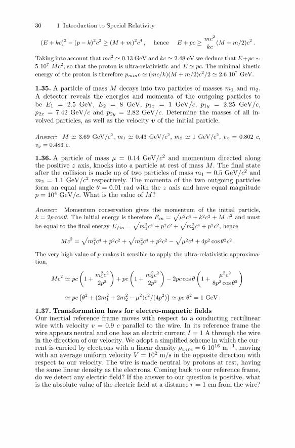
30 1 Introduction to Special Relativity
(E + kc)2 − (p− k)2c2 ≥ (M + m)2c4 , hence E + pc ≥ mc2
kc(M + m/2)c2 .
Taking into account that mc2 � 0.13 GeV and kc � 2.48 eV we deduce that E+pc ∼5 107 Mc2, so that the proton is ultra-relativistic and E � pc. The minimal kinetic
energy of the proton is therefore pminc � (mc/k)(M + m/2)c2/2 � 2.6 107 GeV.
1.35. A particle of mass M decays into two particles of masses m1 and m2.A detector reveals the energies and momenta of the outgoing particles tobe E1 = 2.5 GeV, E2 = 8 GeV, p1x = 1 GeV/c, p1y = 2.25 GeV/c,p2x = 7.42 GeV/c and p2y = 2.82 GeV/c. Determine the masses of all in-volved particles, as well as the velocity v of the initial particle.
Answer: M � 3.69 GeV/c2, m1 � 0.43 GeV/c2, m2 � 1 GeV/c2, vx = 0.802 c,
vy = 0.483 c.
1.36. A particle of mass μ = 0.14 GeV/c2 and momentum directed alongthe positive z axis, knocks into a particle at rest of mass M . The final stateafter the collision is made up of two particles of mass m1 = 0.5 GeV/c2 andm2 = 1.1 GeV/c2 respectively. The momenta of the two outgoing particlesform an equal angle θ = 0.01 rad with the z axis and have equal magnitudep = 104 GeV/c. What is the value of M?
Answer: Momentum conservation gives the momentum of the initial particle,k = 2p cos θ. The initial energy is therefore Ein =
√μ2c4 + k2c2 + M c2 and must
be equal to the final energy Efin =√
m21c
4 + p2c2 +√
m22c
4 + p2c2, hence
Mc2 =√
m21c
4 + p2c2 +√
m22c
4 + p2c2 −√
μ2c4 + 4p2 cos θ2c2 .
The very high value of p makes it sensible to apply the ultra-relativistic approxima-tion,
Mc2 � pc
(1 +
m21c
2
2p2
)+ pc
(1 +
m22c
2
2p2
)− 2pc cos θ
(1 +
μ2c2
8p2 cos θ2
)
� pc(θ2 + (2m2
1 + 2m22 − μ2)c2/(4p2)
)� pc θ2 = 1 GeV .
1.37. Transformation laws for electro-magnetic fieldsOur inertial reference frame moves with respect to a conducting rectilinearwire with velocity v = 0.9 c parallel to the wire. In its reference frame thewire appears neutral and one has an electric current I = 1 A through the wirein the direction of our velocity. We adopt a simplified scheme in which the cur-rent is carried by electrons with a linear density ρwire = 6 1016 m−1, movingwith an average uniform velocity V = 102 m/s in the opposite direction withrespect to our velocity. The wire is made neutral by protons at rest, havingthe same linear density as the electrons. Coming back to our reference frame,do we detect any electric field? If the answer to our question is positive, whatis the absolute value of the electric field at a distance r = 1 cm from the wire?

Problems 31
Answer: If the electrons in the wire are uniformly distributed the distance be-tween two neighboring electrons is d = ρ−1
wire = 1.66 10−17 m in the wire frame.
Due to the length contraction the same distance is d/√
1− (V/c)2 in the elec-tron frame, that is, in a frame moving with respect to the wire with the aver-age electron velocity. Using Einstein formula we compute our velocity with respectto the electron frame v′ = (v + V )/(1 + vV/c2) and the electron density in our
frame: ρmoving,e =√
1− (V/c)2/(d√
1− (v′/c)2) = (1 + vV/c2)/(d√
1− (v/c)2)
while the proton density is ρmoving,p = 1/(d√
1− (v/c)2) ≡ γ/d. Thus the re-
sulting charge density is ρmoving,tot = −evV/(c2d√
1− (v/c)2) = −Iβγ/c wherewe have set β = v/c. Since Maxwell equations are the same in every inertialframe, we conclude that in our frame we have an electric field with absolute valueEmoving = βγI/(2πε0rc) = βγcBwire = 1.23 104 V/m and directed towards thewire. Bwire is the absolute value of the magnetic induction at the same distancefrom the wire in the wire frame; the electric field measured in our frame is or-thogonal with respect to the original magnetic field (in particular it is directed likev ∧Bwire). It also easy to verify that the electric current in our frame is γI , so thatwe measure a magnetic field of absolute value Bmoving = γBwire and parallel to theoriginal magnetic field.
The same results could have been reached using the electro-magnetic field trans-
formation rules; alternatively, the complete set of field transformation rules can be
obtained through the analysis of analogous gedanken experiments. To that purpose
the reader may compute the electric and magnetic fields felt by an observer moving:
a) parallel to a wire having a uniform charge density and zero electric current; b)
parallel to an infinite plane carrying zero charge density and a uniform current den-
sity orthogonal to the observer velocity; c) orthogonal to an infinite plane carrying
uniform charge density and zero electric current.

2
Introduction to Quantum Physics
The gestation of Quantum Physics has been very long and its phenomeno-logical foundations were various. Historically the original idea came from theanalysis of the black body spectrum. This is not surprising since the blackbody, in fact an oven in thermal equilibrium with the electromagnetic radi-ation, is a simple and fundamental system once the law of electrodynamicsare established. As a matter of fact many properties of the spectrum canbe deduced starting from the general laws of electrodynamics and thermody-namics; the crisis came from the violation of the equipartition of energy. Thatsuggested to Planck the idea of quantum, from which everything originated.Of course a long sequence of different discoveries, first of all the photoelectriceffect, the line spectra for atomic emission/absorption, the Compton effectand so on, gave a compelling evidence for the new theory.
Due to the particular limits of the present notes, an exhaustive analysis ofthe whole phenomenology is impossible. Even a clear discussion of the blackbody problem needs an exceeding amount of space. Therefore we have chosena particular line, putting major emphasis on the photoelectric effect and onthe inadequacy of a classical approach based on Thomson’s model of the atom,followed by Bohr’s analysis of the quantized structure of Rutherford’s atomand by the construction of Schrodinger’s theory. This does not mean thatwe have completely overlooked the remaining phenomenology; we have justpresented it in the light of the established quantum theory. Thus, for example,Chapter 3 ends with the analysis of the black body spectrum in the light ofquantum theory.
2.1 The Photoelectric Effect
The photoelectric effect was discovered by H. Hertz in 1887. As sketched inFig. 2.1, two electrodes are placed in a vacuum cell; one of them (C) is hitby monochromatic light of variable frequency, while the second (A) is set to
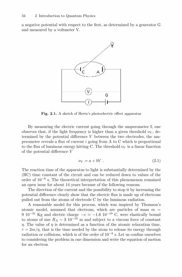
34 2 Introduction to Quantum Physics
a negative potential with respect to the first, as determined by a generator Gand measured by a voltmeter V.
Fig. 2.1. A sketch of Hertz’s photoelectric effect apparatus
By measuring the electric current going through the amperometer I, oneobserves that, if the light frequency is higher than a given threshold νV , de-termined by the potential difference V between the two electrodes, the am-perometer reveals a flux of current i going from A to C which is proportionalto the flux of luminous energy hitting C. The threshold νV is a linear functionof the potential difference V
νV = a + bV . (2.1)
The reaction time of the apparatus to light is substantially determined by the(RC) time constant of the circuit and can be reduced down to values of theorder of 10−8 s. The theoretical interpretation of this phenomenon remainedan open issue for about 14 years because of the following reasons.
The direction of the current and the possibility to stop it by increasing thepotential difference clearly show that the electric flux is made up of electronspulled out from the atoms of electrode C by the luminous radiation.
A reasonable model for this process, which was inspired by Thomson’satomic model, assumed that electrons, which are particles of mass m =9 10−31 Kg and electric charge −e � −1.6 10−19 C, were elastically boundto atoms of size RA ∼ 3 10−10 m and subject to a viscous force of constantη. The value of η is determined as a function of the atomic relaxation time,τ = 2m/η, that is the time needed by the atom to release its energy throughradiation or collisions, which is of the order of 10−8 s. Let us confine ourselvesto considering the problem in one dimension and write the equation of motionfor an electron
2.1 The Photoelectric Effect 35
mx = −kx− ηx− eE , (2.2)
where E is an applied electric field and k is determined on the basis of atomicfrequencies. In particular we suppose the presence of many atoms with differ-ent frequencies continuously distributed around√
k
m= ω0 = 2πν0 ∼ 1015 s−1 . (2.3)
If we assume an oscillating electric field E = E0 cos(ωt) with ω ∼ 1015 s−1,corresponding to visible light, then a general solution to (2.2) is given by
x = x0 cos(ωt + φ) + A1e−α1t + A2e
−α2t , (2.4)
where the second and third term satisfy the homogeneous equation associatedwith (2.2), so that α1/2 are the solutions of the following equation
mα2 − ηα + k = 0 ,
α =η ±
√η2 − 4km
2m=
1
τ±√
1
τ2− ω2
0 �1
τ± i ω0 , (2.5)
where last approximation is due to the assumption τ � ω−10 .
Regarding the particular solution x0 cos(ωt+φ), we obtain by substitution:
−mω2x0 cos(ωt+φ) = −kx0 cos(ωt+φ)+ηωx0 sin(ωt+φ)−eE0 cos(ωt) (2.6)
hence
(k −mω2)x0 (cos(ωt) cosφ− sin(ωt) sin φ)
= ηωx0 (sin(ωt) cosφ + cos(ωt) sinφ) − eE0 cos(ωt)
from which, by taking alternatively ωt = 0, π/2, we obtain the following sys-tem (
m(ω2
0 − ω2)cosφ− ηω sinφ
)x0 = −eE0 ,
m(ω2
0 − ω2)x0 sin φ + ηω x0 cosφ = 0 (2.7)
which can be solved for φ
tan φ =2ω
τ (ω2 − ω20)
,
cosφ =ω2 − ω2
0√(ω2
0 − ω2)2
+ 4ω2
τ2
, sin φ =(2ω/τ)√
(ω20 − ω2)
2+ 4ω2
τ2
(2.8)
and finally for x0, for which we obtain the well known resonant form

36 2 Introduction to Quantum Physics
x0 =eE0/m√
(ω20 − ω2)
2+ 4ω2
τ2
. (2.9)
To complete our computation we must determine A1 and A2. On the otherhand, taking into account (2.5) and the fact that x is real, we can rewrite thegeneral solution in the following equivalent form:
x = x0 cos(ωt + φ) + Ae−t/τ cos(ω0t + φ0) . (2.10)
If we assume that the electron be initially at rest, we can determine A and φ0
by taking x = x = 0 for t = 0, i.e.
x0 cosφ + A cosφ0 = 0 , (2.11)
x0 ω sin φ = −A
(cosφ0
τ+ ω0 sin φ0
), (2.12)
hence in particular
tan φ0 =ω
ω0tanφ− 1
ω0τ. (2.13)
These equations give us enough information to discuss the photoelectric effectwithout explicitly substituting A in (2.10).
Indeed in our simplified model the effect, i.e. the liberation of the electronfrom the atomic bond, happens as the amplitude of the electron displacementx is greater than the atomic radius. In equation (2.10) x is the sum of twoparts, the first corresponding to stationary oscillations, the second to a tran-sient decaying with time constant τ . In principle, the maximum amplitudecould take place during the transient or later: to decide which is the case wemust compare the value of A with that of x0. It is apparent from (2.11) thatthe magnitude of A is of the same order as x0 unless cosφ0 is much less thancosφ. On the other hand, equation (2.13) tells us that, if tanφ0 is large, thentan φ is large as well, since (ω0τ)−1 ∼ 10−7 and ω/ω0 ∼ 1. Therefore, theorder of magnitude of the maximum displacement is given by x0, and can besensitive to the electric field frequency. That happens in the resonant regime,where ω differs from ω0 by less than 2
√ω/τ .
Let us consider separately the generic case from the resonant one. In thefirst case the displacement is of the order of eE0/(ω2m), since the square rootof the denominator in (2.9) has the same order of magnitude as ω2. In orderto induce the photoelectric effect it is therefore necessary that
eE0
ω2m∼ RA ,
from which we can compute the power density needed for the luminous beamwhich hits electrode C:
P = cε0E20 ∼ cε0
(RAω2m
e
)2
,
2.1 The Photoelectric Effect 37
where c is the speed of light and ε0 is the vacuum dielectric constant. P comesout to be of the order of 1015 W/m2, a power density which is difficult torealize in practice and which would anyway be enough to vaporize any kind ofelectrode. We must conclude that our model cannot explain the photoelectriceffect if ω is far from resonance. Let us consider therefore the resonant caseand set ω = ω0. On the basis of (2.11), (2.13) and (2.9), that implies:
φ = φ0 =π
2, A = −x0 ,
hence
x =−eE0τ
2mω0
(1− e−t/τ
)sin(ω0t) . (2.14)
In order for the photoelectric effect to take place, the oscillation amplitudemust be greater than the atomic radius:
eE0τ
2mω0
(1− e−t/τ
)≥ RA .
That sets the threshold field to 2mω0RA/(eτ) and the power density of thebeam to
P = cε0
(4ω0mRA
τe
)2
∼ 100 W/m2 ,
while the time required to reach the escape amplitude is of the order of τ .In conclusion, our model predicts a threshold for the power of the beam,
but not for its frequency, which however must be tuned to the resonancefrequency: the photoelectric effect would cease both below and above thetypical resonance frequencies of the atoms in the electrode. Moreover theexpectation is that the electron does not gain any further appreciable energyfrom the electric field once it escapes the atomic bond: hence the emission fromthe electrode could be strong, but made up of electrons of energy equal to thatgained during the last atomic oscillation. Equation (2.14) shows that, duringthe transient (t << τ), the oscillation amplitude grows roughly by eE0/(mω2
0)in one period, so that the energy of the escaped electron would be of the orderof magnitude of kRAeE0/(mω2
0) = eE0RA, corresponding also to the energyacquired by the electron from the electric field E0 when crossing the atom. Itis easily computed that for a power density of the order of 10 − 100 W/m2,the electric field E0 is roughly 100 V/m, so that the final kinetic energy ofthe electron would be 10−8 eV ∼ 10−27 J: this value is much smaller than thetypical thermal energy at room temperature (3kT/2 ∼ 10−1 eV).
The prediction of the model is therefore in clear contradiction with theexperimental results described above. In particular the very small energy ofthe emitted electrons implies that the electric current I should vanish evenfor small negative potential differences.
Einstein proposed a description of the effect based on the hypothesis thatthe energy be transferred from the luminous radiation to the electron in a

38 2 Introduction to Quantum Physics
single elementary (i.e. no further separable) process, instead than through agradual excitation. Moreover he proposed that the transferred energy be equalto hν = hω/(2π) ≡ hω, a quantity called quantum by Einstein himself. Theconstant h had been introduced by Planck several years before to describe theradiation emitted by an oven and its value is 6.63 10−34 J s.
If the quantum of energy is enough for electron liberation, i.e. according toour model it is larger than Et ≡ kR2
A/2 = ω20R
2Am/2 ∼ 10−19 J ∼ 1 eV, and
the frequency exceeds 1.6 1014 Hz (corresponding to ω in our model), thenthe electron is emitted keeping the energy exceeding the threshold in the formof kinetic energy. The number of emitted electrons, hence the intensity of theprocess, is proportional to the flux of luminous energy, i.e. to the number ofquanta hitting the electrode.
Since E = hν is the energy gained by the electron, which spends a part Et
to get free from the atom, the final electron kinetic energy is T = hν −Et, sothat the electric current can be interrupted by placing the second electrodeat a negative potential
V =hν − Et
e,
thus reproducing (2.1).The most important point in Einstein’s proposal, which was already no-
ticed by Planck, is that a physical system of typical frequency ν can exchangeonly quanta of energy equal to hν. The order of magnitude in the atomic caseis ω ∼ 1015 s−1, hence hω ≡ (h/2π) ω ∼ 1 eV.
2.2 Bohr’s Quantum Theory
After the introduction of the concept of a quantum of energy, quantum theory
was developed by N. Bohr in 1913 and then perfected by A. Sommerfeld in1916: they gave a precise proposal for multi-periodic systems, i.e. systemswhich can be described in terms of periodic components.
The main purpose of their studies was that of explaining, in the frameworkof Rutherford’s atomic model, the light spectra emitted by gasses (in partic-ular mono-atomic ones) excited by electric discharges. The most simple andrenowned case is that of the mono-atomic hydrogen gas (which can be pre-pared with some difficulties since hydrogen tends to form diatomic molecules).It has a discrete spectrum, i.e. the emitted frequencies can assume only somediscrete values, in particular:
νn,m = R
(1
n2− 1
m2
)(2.15)
for all possible positive integer pairs with m > n: this formula was first pro-posed by J. Balmer in 1885 for the case n = 2, m ≥ 3, and then generalized byJ. Rydberg in 1888 for all possible pairs (n, m). The emission is particularlystrong for m = n + 1.
2.2 Bohr’s Quantum Theory 39
Rutherford had shown that the positive charge in an atom is localized in apractically point-like nucleus, which also contains most of the atomic mass. Inparticular the hydrogen atom can be described as a two-body system: a heavyand positively charged particle, which nowadays is called proton, bound byCoulomb forces to a light and negatively charged particle, the electron.
We will confine our discussion to the case of circular orbits of radius r,covered with uniform angular velocity ω, and will consider the proton as if itwere infinitely heavy (its mass is about 2 103 times that of the electron). Inthis case we have
mω2r =e2
4πε0r2,
where m is the electron mass. Hence the orbital frequencies, which in clas-sical physics correspond to those of the emitted radiation, are continuouslydistributed as a function of the radius
ν =ω
2π=
e√16π3ε0mr3
; (2.16)
this is in clear contradiction with (2.15). Based on Einstein’s theory of thephotoelectric effect, Bohr proposed to interpret (2.15) by assuming that onlycertain orbits be allowed in the atom, which are called levels, and that thefrequency νn,m correspond to the transition from the m-th level to n-th one.In that case
hνn,m = Em − En , (2.17)
where the atomic energies (which are negative since the atom is a boundsystem) would be given by
En = −hR
n2. (2.18)
Since, according to classical physics for the circular orbit case, the atomicenergy is given by
Ecirc = − e2
8πε0r,
Bohr’s hypothesis is equivalent to the assumption that the admitted orbitalradii be
rn =e2n2
8πε0hR. (2.19)
It is clear that Bohr’s hypothesis seems simply aimed at reproducing theobserved experimental data; it does not permit any particular further devel-opment, unless further conditions are introduced. The most natural, which iscalled correspondence principle, is that the classical law, given in (2.16), bereproduced by (2.15) for large values of r, hence of n, and at least for thestrongest emissions, i.e. those with m = n + 1, for which we can write
νn,n+1 = R2n + 1
n2(n + 1)2→ 2R
n3, (2.20)
40 2 Introduction to Quantum Physics
these frequencies should be identified in the above mentioned limit with whatresulting from the combination of (2.16) and (2.19):
ν =e√
16π3ε0mr3n
=ε0√
32(hR)3
e2√
mn3. (2.21)
By comparing last two equations we get the value of the coefficient R in (2.15),which is called Rydberg constant:
R =me4
8ε20h3
and is in excellent agreement with experimental determinations. We have thenthe following quantized atomic energies
En = − me4
8ε20h2n2
, n = 1, 2, ...
while the quantized orbital radii are
rn =ε0h
2n2
πme2. (2.22)
In order to give a numerical estimate of our results, it is convenient to intro-duce the ratio e2/(2ε0hc) ≡ α � 1/137, which is dimensionless and is knownas the fine structure constant. The energy of the state with n = 1, which iscalled the ground state, is
E1 = −hR = −mc2
2α2 ;
noticing that mc2 ∼ 0.51 MeV, we have E1 � −13.6 eV. The correspondingatomic radius (Bohr radius) is r1 � 0.53 10−10 m.
Notwithstanding the excellent agreement with experimental data, thestarting hypothesis, to be identified with (2.18), looks still quite conditionedby the particular form of Balmer law given in (2.15). For that reason Bohrtried to identify a physical observable to be quantized according to a simplerand more fundamental law. He proceeded according to the idea that such ob-servable should have the same dimensions of the Planck constant, i.e. thoseof an action, or equivalently of an angular momentum. In the particular caseof quantized circular orbits this last quantity reads:
L = pr = mωr2 =e√
4πε0
√mrn =
h
2πn ≡ nh , n = 1, 2, ... . (2.23)
2.3 De Broglie’s Interpretation
In this picture of partial results, even if quite convincing from the point ofview of the phenomenological comparison, the real progress towards under-standing quantum physics came as L. de Broglie suggested the existence of a
2.3 De Broglie’s Interpretation 41
universal wave-like behavior of material particles and of energy quanta asso-ciated to force fields. As we have seen in the case of electromagnetic waveswhen discussing the Doppler effect, a phase can always be associated with awave-like process, which is variable both in space and in time (e.g. given by2π (x/λ− νt) in the case of waves moving parallel to the x axis). The assump-tion that quanta can be interpreted as real particles and that Einstein’s lawE = hν be universally valid, would correspond to identifying the wave phasewith 2π (x/λ− Et/h). If we further assume the phase to be relativisticallyinvariant, then it must be expressed in the form (p x− E t) /h, where E andp are identified with relativistic energy and momentum, i.e. in the case ofmaterial particles:
E =mc2√(1− v2
c2
) , p =mv√(1− v2
c2
) .
In order to simplify the discussion as much as possible, we will consider hereand in most of the following a one-dimensional motion (parallel to the x axis).In conclusion, by comparing last two expressions given for the phase, we obtainde Broglie’s equation:
p =h
λ,
which is complementary to Einstein’s law, E = hν.These formulae give an idea of the scale at which quantum effects are
visible. For an electron having kinetic energy Ek = 102 eV � 1.6 10−17 J,quantum effects show up at distances of the order of λ = h/p = h/
√2mEk ∼
10−10 m, corresponding to atomic or slightly subatomic distances; that con-firms the importance of quantum effects for electrons in condensed matter andin particular in solids, where typical energies are of the order of a few electron-volts. For a gas of light atoms in equilibrium at temperature T , the kineticenergy predicted by equipartition theorem is 3kT/2, where k is Boltzmann’sconstant. At a temperature T = 300◦K (room temperature) the kinetic energyis roughly 2.5 10−2 eV, corresponding to wavelengths of about 10−10 m foratom masses of the order of 10−26 Kg. However at those distances the pictureof a non-interacting (perfect) gas does not apply because of strong repulsiveforces coming into play: in order to gain a factor ten on distances, it is neces-sary to reduce the temperature by a factor 100, going down to a few Kelvindegrees, at which quantum effects are manifest. For a macroscopic body ofmass 1 Kg and kinetic energy 1 J quantum effects would show up at distancesroughly equal to 3 10−34 m, hence completely negligible with respect to thethermal oscillation amplitudes of atoms, which are proportional to the squareroot of the absolute temperature, and are in particular of the order of a fewnanometers at T = 103 ◦K, where the solid melts.
On the other hand, Einstein’s formula gives us information about the scaleof times involved in quantum processes, which is of the order of h/ΔE, whereΔE corresponds to the amount of exchanged energy. For ΔE ∼ 1 eV, times
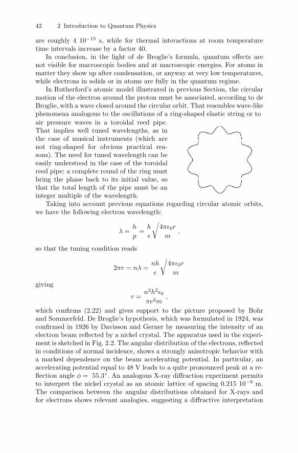
42 2 Introduction to Quantum Physics
are roughly 4 10−15 s, while for thermal interactions at room temperaturetime intervals increase by a factor 40.
In conclusion, in the light of de Broglie’s formula, quantum effects arenot visible for macroscopic bodies and at macroscopic energies. For atoms inmatter they show up after condensation, or anyway at very low temperatures,while electrons in solids or in atoms are fully in the quantum regime.
In Rutherford’s atomic model illustrated in previous Section, the circularmotion of the electron around the proton must be associated, according to deBroglie, with a wave closed around the circular orbit. That resembles wave-likephenomena analogous to the oscillations of a ring-shaped elastic string or to
air pressure waves in a toroidal reed pipe.That implies well tuned wavelengths, as inthe case of musical instruments (which arenot ring-shaped for obvious practical rea-sons). The need for tuned wavelength can beeasily understood in the case of the toroidalreed pipe: a complete round of the ring mustbring the phase back to its initial value, sothat the total length of the pipe must be aninteger multiple of the wavelength.
Taking into account previous equations regarding circular atomic orbits,we have the following electron wavelength:
λ =h
p=
h
e
√4πε0r
m,
so that the tuning condition reads
2πr = nλ =nh
e
√4πε0r
m
giving
r =n2h2ε0πe2m
,
which confirms (2.22) and gives support to the picture proposed by Bohrand Sommerfeld. De Broglie’s hypothesis, which was formulated in 1924, wasconfirmed in 1926 by Davisson and Gerner by measuring the intensity of anelectron beam reflected by a nickel crystal. The apparatus used in the experi-ment is sketched in Fig. 2.2. The angular distribution of the electrons, reflectedin conditions of normal incidence, shows a strongly anisotropic behavior witha marked dependence on the beam accelerating potential. In particular, anaccelerating potential equal to 48 V leads to a quite pronounced peak at a re-flection angle φ = 55.3◦. An analogous X-ray diffraction experiment permitsto interpret the nickel crystal as an atomic lattice of spacing 0.215 10−9 m.The comparison between the angular distributions obtained for X-rays andfor electrons shows relevant analogies, suggesting a diffractive interpretation
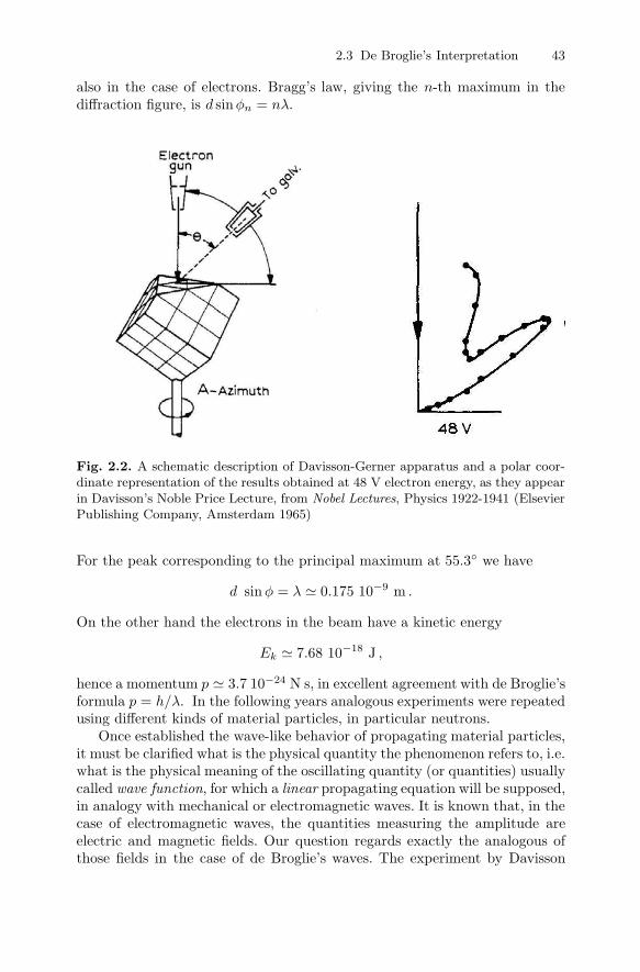
2.3 De Broglie’s Interpretation 43
also in the case of electrons. Bragg’s law, giving the n-th maximum in thediffraction figure, is d sinφn = nλ.
Fig. 2.2. A schematic description of Davisson-Gerner apparatus and a polar coor-dinate representation of the results obtained at 48 V electron energy, as they appearin Davisson’s Noble Price Lecture, from Nobel Lectures, Physics 1922-1941 (ElsevierPublishing Company, Amsterdam 1965)
For the peak corresponding to the principal maximum at 55.3◦ we have
d sin φ = λ � 0.175 10−9 m .
On the other hand the electrons in the beam have a kinetic energy
Ek � 7.68 10−18 J ,
hence a momentum p � 3.7 10−24 N s, in excellent agreement with de Broglie’sformula p = h/λ. In the following years analogous experiments were repeatedusing different kinds of material particles, in particular neutrons.
Once established the wave-like behavior of propagating material particles,it must be clarified what is the physical quantity the phenomenon refers to, i.e.what is the physical meaning of the oscillating quantity (or quantities) usuallycalled wave function, for which a linear propagating equation will be supposed,in analogy with mechanical or electromagnetic waves. It is known that, in thecase of electromagnetic waves, the quantities measuring the amplitude areelectric and magnetic fields. Our question regards exactly the analogous ofthose fields in the case of de Broglie’s waves. The experiment by Davisson

44 2 Introduction to Quantum Physics
and Gerner gives an answer to this question. Indeed, as illustrated in Fig. 2.2,the detector reveals the presence of one or more electrons at a given angle; ifwe imagine to repeat the experiment several times, with a single electron inthe beam at each time, and if we measure the frequency at which electrons aredetected at the various angles, we get the probability of having the electron ina given site covered by the detector.
In the case of an optical measure, what is observed is the interference effectin the energy deposited on a plate; that is proportional to the square of theelectric field on the plate. Notice that the linearity in the wave equation andthe quadratic relation between the measured quantity and the wave ampli-tude are essential conditions for the existence of interference and diffractivephenomena. We must conclude that also in the case of material particles somepositive quadratic form of the de Broglie wave function gives the probabilityof having the electron in a given point.
We have quite generically mentioned a quadratic form, since at the mo-ment it is still not clear if the wave function has one or more components, i.e.if it corresponds to one or more real functions. By a positive quadratic formwe mean a homogeneous second order polynomial in the wave function com-ponents, which is positive for real and non-vanishing values of its arguments.In the case of a single component, we can say without loss of generality thatthe probability density is the wave function squared, while in the case of twoor more components it is always possible, by suitable linear transformations,to reduce the quadratic form to a sum of squares.
We are now going to show that the hypothesis of a single component mustbe discarded. Let us indicate by ρ(r, t)d3r the probability of the particle beingin a region of size d3r around r at time t, and by ψ(r, t) the wave function,which for the moment is considered as a real valued function, defined so that
ρ(r, t) = ψ2(r, t) . (2.24)
If Ω indicates the whole region accessible to the particle, the probability den-sity must satisfy the natural constraint:∫
Ω
d3rρ (r, t) = 1 , (2.25)
which implies the condition:∫Ω
d3r ρ(r, t) ≡∫
Ω
d3r∂ρ(r, t)
∂t= 0 . (2.26)
This expresses the fact that, if the particle cannot escape Ω, the probabilityof finding it in that region must always be one. This condition can be givenin mathematical terms analogous to those used to express electric chargeconservation: the charge contained in a given volume, i.e. the integral of thecharge density, may change only if the charge flows through the boundarysurface. The charge flux through the boundaries is expressed in terms of the

2.3 De Broglie’s Interpretation 45
current density flow and can be rewritten as the integral of the divergence ofthe current density itself by using Gauss–Green theorem∫
Ω
ρ = −Φ∂Ω(J) = −∫
Ω
∇ · J .
Finally, by reducing the equation from an integral form to a differential one,we can set the temporal derivative of the charge density equal to minus thedivergence of the current density. Based on this analogy, let us introduce theprobability current density J and write
ρ(r, t) = −∂Jx(r, t)
∂x− ∂Jy(r, t)
∂y− ∂Jz(r, t)
∂z≡ −∇ · J(r, t) . (2.27)
The conservation equation must be automatically satisfied as a consequenceof the propagation equation of de Broglie’s waves, which we write in the form:
ψ = L(ψ, ∇ψ,∇2ψ, . . .
), (2.28)
where L indicates a generic linear function of ψ and its derivatives like:
L(ψ, ∇ψ,∇2ψ, . . .
)= αψ + β∇2ψ . (2.29)
Notice that if L were not linear the interference mechanism upon which quan-tization is founded would soon or later fail. Furthermore we assume invarianceunder the reflection of the coordinates, at least in the free case, so that termsproportional to first derivatives are excluded.
From equation (2.24) we have ρ = 2ψψ, which can be rewritten, using(2.28), as:
ρ = 2ψL(ψ, ∇ψ,∇2ψ, . . .
). (2.30)
The right-hand side of last equation must be identified with−∇·J(r, t). More-over J must necessarily be a bilinear function of ψ and its derivatives, exactlylike ρ. Therefore, since J is a vector-like quantity, it must be expressible as
J = c ψ∇ψ + d ∇ψ∇2ψ + . . .
from which it appears that ∇ ·J(r, t) must necessarily contain bilinear termsin which both functions are derived, like ∇ψ ·∇ψ: however such terms areclearly missing in (2.30).
We come to the conclusion that the description of de Broglie’s waves re-quires at least two wave functions ψ1 and ψ2, defined so that ρ = ψ2
1 + ψ22 . In
an analogous way we can introduce the complex valued function:
ψ = ψ1 + iψ2 , (2.31)
defined so thatρ = |ψ|2 ; (2.32)

46 2 Introduction to Quantum Physics
this choice implies:ρ = ψ∗ψ + ψψ∗ .
If we assume, for instance, the wave equation corresponding to (2.29):
ψ = αψ + β∇2ψ , (2.33)
we obtain:ρ = ψ∗
(αψ + β∇2ψ
)+ ψ
(α∗ψ∗ + β∗∇2ψ∗
).
If we also assume that the probability current density be
J = ik (ψ∗∇ψ − ψ∇ψ∗) , (2.34)
with k real so as to make J real as well, we easily derive
∇ · J = ik(ψ∗∇2ψ − ψ∇2ψ∗
).
It can be easily verified that the continuity equation (2.27) is satisfied if
α + α∗ = 0 , β = −ik . (2.35)
It is of great physical interest to consider the case in which the wave func-tion has more than two real components. In particular, the wave function ofelectrons has four components or, equivalently, two complex components. Ingeneral, the multiplicity of the complex components is linked to the existenceof an intrinsic angular momentum, which is called spin. The various complexcomponents are associated with the different possible spin orientations. In thecase of particles with non-vanishing mass, the number of components is 2S+1,where S is the spin of the particle. In the case of the electron, S = 1/2 .
For several particles, as for the electron, spin is associated with a magneticmoment which is inherent to the particle: it behaves as a microscopic magnetwith various possible orientations, corresponding to those of the spin, whichcan be selected by placing the particle in a non-uniform magnetic field andmeasuring the force acting on the particle.
2.4 Schrodinger’s Equation
The simplest case to which our considerations can be applied is that of a non-relativistic free particle of mass m. To simplify notations and computations,we shall confine ourselves to a one-dimensional motion, parallel for instance tothe x axis; if the particle is not free, forces will be parallel to the same axis aswell. The obtained results will be extensible to three dimensions by exploitingthe vector formalism. In practice, we shall replace ∇ by its component ∇x =∂/∂x ≡ ∂x and the Laplacian operator ∇2 = ∂2/∂x2 + ∂2/∂y2 + ∂2/∂z2 by∂2/∂x2 ≡ ∂2
x; the probability current density J will be replaced by Jx (J) aswell. The inverse replacement will suffice to go back to three dimensions.

2.4 Schrodinger’s Equation 47
The energy of a non-relativistic free particle is
E = c√
m2c2 + p2 � mc2 +p2
2m+ O
(p4
m3c2
),
where we have made explicit our intention to neglect terms of the order ofp4/(m3c2). Assuming de Broglie’s interpretation, we write the wave function:
ψP (x, t) ∼ e2πi(x/λ−νt) = ei(px−Et)/h (2.36)
(we are considering a motion in the positive x direction). Our choice impliesthe following wave equation
ψP = − iE
hψP = − i
h
(mc2 +
1
2mp2
)ψP . (2.37)
We have also
∂xψP =i
hpψP , (2.38)
from which we deduce
ihψP = mc2ψP − h2
2m∂2
xψP . (2.39)
Our construction can be simplified by multiplying the initial wave functionby the phase factor eimc2t/h, i.e. defining
ψ ≡ eimc2t/hψP ∼ exp
(i
h
(px− p2
2mt
)). (2.40)
Since the dependence on x is unchanged, ψ still satisfies (2.38) and has thesame probabilistic interpretation as ψP . Indeed both ρ and J are unchanged.The wave equation instead changes:
ihψ = − h2
2m∂2
xψ ≡ Tψ . (2.41)
This is the Schrodinger equation for a free (non-relativistic) particle, in whichthe right-hand side has a natural interpretation in terms of the particle energy,which in the free case is only of kinetic type.
In the case of particles under the influence of a force field correspondingto a potential energy V (x), the equation can be generalized by adding V (x)to the kinetic energy :
ihψ = − h2
2m∂2
xψ + V (x)ψ . (2.42)
This is the one-dimensional Schrodinger equation that we shall apply to var-ious cases of physical interest.
48 2 Introduction to Quantum Physics
Equations (2.34) and (2.35) show that the probability current density doesnot depend on V and is given by:
J = − ih
2m(ψ∗∂xψ − ψ∂xψ∗) . (2.43)
Going back to the free case and considering the plane wave function given in(2.36), it is interesting to notice that the corresponding probability density,ρ = |ψ|2, is a constant function. This result is paradoxical since, by reducing(2.25) to one dimension, we obtain∫ ∞
−∞dx ρ(x, t) =
∫ ∞
−∞dx |ψ(x, t)|2 = 1 , (2.44)
which cannot be satisfied in the examined case, since the integral of a constantfunction is divergent. We must conclude that our interpretation excludes thepossibility that a particle have a well defined momentum.
We are left with the hope that this difficulty may be overcome by admit-ting some (small) uncertainty on the knowledge of momentum. This possibilitycan be easily analyzed thanks to the linearity of Schrodinger equation. Indeedequation (2.41) admits other different solutions besides the simple plane wave,in particular the wave packet solution, which is constructed as a linear super-position of many plane waves according to the following integral:∫ ∞
−∞dp ψ(p) exp
(i
h
(px− p2
2mt
)).
The squared modulus of the superposition coefficients, |ψ(p)|2, can be nat-urally interpreted, apart from a normalization constant, as the probabilitydensity in terms of momentum, exactly in the same way as ρ(x) is interpretedas a probability density in terms of position.
Let us choose in particular a Gaussian distribution:
ψ(p) ∼ e−(p−p0)2/(4Δ2) , (2.45)
corresponding to
ψΔ(x, t) = k
∫ ∞
−∞dp e−(p−p0)2/(4Δ2) ei(px−p2t/2m)/h , (2.46)
where k must be determined in such a way that∫∞−∞ dx|ψΔ(x, t)|2 = 1.
The integral in (2.46) can be computed by recalling that, if α is a complexnumber with positive real part (Re(α) > 0), then∫ ∞
−∞dp e−αp2
=
√π
α
and that the Riemann integral measure dp is left invariant by translations inthe complex plane,

2.4 Schrodinger’s Equation 49∫ ∞
−∞dp e−αp2 ≡
∫ ∞
−∞d(p + γ) e−α(p+γ)2
=
∫ ∞
−∞dp e−α(p+γ)2 = e−αγ2
∫ ∞
−∞dp e−αp2
e−2αγp ,
for every complex number γ. Therefore we have∫ ∞
−∞dp e−αp2
eβp =
√π
αeβ2/4α . (2.47)
Developing (2.46) with the help of (2.47) we can write
ψΔ(x, t) = ke−p20
4Δ2
∫ ∞
−∞dp e−[ 1
4Δ2 + it2mh ]p2
e[p0
2Δ2 + ixh ]p
= k
√π
14Δ2 + it
2mh
exp
([p0
2Δ2 + ixh
]21
Δ2 + 2itmh
− p20
4Δ2
). (2.48)
We are interested in particular in the x dependence of the probability densityρ(x): that is solely related to the real part of the exponent of the rightmostterm in (2.48), which can be expanded as follows:
p20
4Δ4 + ip0xΔ2h − x2
h2
1Δ2 + 2it
mh
− p20
4Δ2= − p2
0
4Δ2
4t2Δ4
m2h2 + 2itΔ2
mh
1 + 4t2Δ4
m2h2
−(
Δ2x2
h2 − ip0x
h
)1− 2itΔ2
mh
1 + 4t2Δ4
m2h2
the real part being
− Δ2(x− p0t
m
)2h2(1 + 4t2Δ4
m2h2
) ≡ − Δ2 (x− v0t)2
h2(1 + 4t2Δ4
m2h2
) .
Since p0 is clearly the average momentum of the particle, we have introducedthe corresponding average velocity v0 = p0/m. Recalling the definition of ρ,as well as its normalization constraint, we finally find
ρ(x, t) =Δ
h
√2
π(1 + 4t2Δ4
m2h2
) exp
(−2Δ2
h2
(x− v0t)2
1 + 4t2Δ4
m2h2
), (2.49)
while the probability distribution in terms of momentum reads
ρ(p) =1√2πΔ
e−(p−p0)2/(2Δ2) . (2.50)
Given a Gaussian distribution ρ(x) = 1/(√
2πσ)e−(x−x0)2/(2σ2), it is a well
known fact, which anyway can be easily derived from previous formulae, thatthe mean value x is x0 while the mean quadratic deviation (x− x)2 is equalto σ2. Hence, in the examined case, we have an average position x = v0t

50 2 Introduction to Quantum Physics
with a mean quadratic deviation equal to h2/(4Δ2) + t2Δ2/m2, while theaverage momentum is p0 with a mean quadratic deviation Δ2. The meanvalues represent the kinematic variables of a free particle, while the meanquadratic deviations are roughly inversely proportional to each other: if weimprove the definition of one observable, the other becomes automatically lessdefined.
The former results can be derived in a shorter way and generalized usingthe stationary phase approximation that we briefly present here. Suppose wewant to compute an integral of the form:∫ ∞
−∞dq exp(−F (q, ξ)) , (2.51)
where ξ stands for a set of parameters, e.g. x and t, and F (q, ξ) is a complexvalued function whose real part tends to ∞ when |q| → ∞. Let F (z, ξ) be ananalytic extension of F (q, ξ), that is an analytic function in z in a suitabledomain D neighboring the real axis, that is, such that limε→0 F (q ± iε, ξ) =F (q, ξ) for a suitable choice of the sign.
Suppose furthermore that the equation ∂zF (z, ξ) = 0 has a finite numberof solutions z1, . . . , zn in D and that |∂2
z F (z1, ξ)| � |∂2z F (zi, ξ)| for any i > 1.
Then the integral (2.51) is approximated by
∫ ∞
−∞dq exp(−F (q, ξ)) �
√2π
∂2z F (z1, ξ)
exp(−F (z1, ξ)), (2.52)
and the approximation improves so long as the inequality becomes stronger.In the case of the Gaussian wave packet the reader should verify that the
equation ∂zF (z, ξ) = 0 has a single solution and hence (2.52) becomes anidentity.
The distributions given in (2.49) and (2.50), even if derived in the contextof a particular example, permit to reach important general conclusions which,for the sake of clarity, are listed in the following as distinct points.
2.4.1 The Uncertainty Principle
While the mean quadratic deviation relative to the momentum distribution
(p− p)2 = Δ2
has been fixed a-priori by choosing ψ(p) and is independent of time, thusconfirming that momentum is a constant of motion for a free particle, thatrelative to the position
(x − x)2 =
(1 +
4t2Δ4
m2h2
)h2
4Δ2

2.4 Schrodinger’s Equation 51
does not contain further free parameters and does depend on time. Indeed,Δx grows significantly for 2tΔ2/(mh) > 1, hence for times greater thants = mh/(2Δ2). Notice that ts is nothing but the time needed for a par-ticle of momentum Δ to cover a distance h/(2Δ), therefore this spreading hasa natural interpretation also from a classical point of view: a set of indepen-dent particles having momenta distributed according to a width Δp, spreadswith velocity Δp/m = vs; if the particles are statistically distributed in aregion of size initially equal to Δx, the same size will grow significantly aftertimes of the order of Δx/vs.
What is new in our results is, first of all, that they refer to a single parti-cle, meaning that uncertainties in position and momentum are not avoidable;secondly, these uncertainties are strictly interrelated. Without considering thespreading in time, it is evident that the uncertainty in one variable can bediminished only as the other uncertainty grows. Indeed, Δ can be eliminatedfrom our equations by writing the inequality:
ΔxΔp ≡√
(x− x)2 (p− p)2 ≥ h
2, (2.53)
which is known as the Heinsenberg uncertainty principle and can be shownto be valid for any kind of wave packet. The case of a real Gaussian packetcorresponds to the minimal possible value ΔxΔp = h/2.
From a phenomenological point of view this principle originates from theuniversality of diffractive phenomena. Indeed diffractive effects are those whichprevent the possibility of a simultaneous measurement of position and mo-mentum with arbitrarily good precision for both quantities. Let us considerfor instance the case in which the measurement is performed through opticalinstruments; in order to improve the resolution it is necessary to make useof radiation of shorter wavelength, thus increasing the momenta of photons,which hitting the object under observation change its momentum in an un-predictable way. If instead position is determined through mechanical instru-ments, like slits, then the uncertainty in momentum is caused by diffractivephenomena.
It is important to evaluate the order of magnitude of quantum uncertaintyin cases of practical interest. Let us consider for instance a beam of electronsemitted by a cathode at a temperature T = 1000◦K and accelerated througha potential difference equal to 104 V. The order of magnitude of the kineticenergy uncertainty ΔE is kT , where k = 1.381 10−23 J/◦K is the Boltz-mann constant (alternatively one can use k = 8.617 10−5 eV/◦K ). ThereforeΔE = 1.38 10−20 J, while E = 1.6 10−15 J, corresponding to a quite precisedetermination of the beam energy (ΔE/E ∼ 10−5). We can easily computethe momentum uncertainty by using error propagation (Δp/p = 1
2ΔE/E) andcomputing p =
√2meE = 5.6 10−23 N s; we thus obtain Δp = 2.8 10−28 N s,
hence, making use of (2.53), Δx ≥ 2 10−7 m. It is clear that the uncertaintyprinciple does not place significant constraints in this case.

52 2 Introduction to Quantum Physics
A macroscopic body of mass M = 1 Kg placed at room temperature(T � 300◦K) has an average thermal momentum, caused by collisions withair molecules, which is equal to Δp ∼
√2M 3kT/2 � 9 10−11 N s, so that
the minimal quantum uncertainty on its position is Δx ∼ 10−24 m, hence notappreciable.
The uncertainty principle is instead quite relevant at the atomic level,where it is the stabilizing mechanism which prevents the electron from collaps-ing onto the nucleus. We can think of the electron orbital radius as a rough es-timate of its position uncertainty (Δx ∼ r) and evaluate the kinetic energy de-riving from the momentum uncertainty; we have Ek ∼ Δ2
p/(2m) ∼ h2/(2mr2).Taking into account the binding Coulomb energy, the total energy is
E(r) ∼ h2
2mr2− e2
4πε0r.
We infer that the system is stable, since the total energy E(r) has an abso-lute minimum. The stable radius rm corresponding to this minimum can becomputed through the equation
e2
4πε0r2m
− h2
mr3m
= 0 ,
hence
rm ∼ 4πε0h2
me2,
which nicely reproduce the value of the atomic radius for the fundamentallevel in Bohr’s model, see equation (2.22).
2.4.2 The Speed of Waves
It is known that electromagnetic waves move without distortion at a speedc = 1/
√ε0μ0 and that, for a harmonic wave, c is given by the wavelength
multiplied by the frequency.In the case of de Broglie’s waves, equation (2.40), we have ν = p2/(2mh)
and λ = h/p; therefore the velocity of harmonic waves is given by vF ≡λν = p/(2m). If we consider instead the wave packet given in (2.48) and itscorresponding probability density given in (2.49), we clearly see that it moveswith a velocity vG ≡ p0/m, which is equal to the classical velocity of a par-ticle with momentum p0. We have used different symbols to distinguish thevelocity of plane waves vF , which is called phase velocity, from vG, which isthe speed of the packet and is called group velocity. Previous equations leadto the result that, contrary to what happens for electromagnetic waves prop-agating in vacuum, the two velocities are different for de Broglie’s waves, andin particular the group velocity does not coincide with the average value of thephase velocities of the different plane waves making up the packet. Moreover,the phase velocity depends on the wavelength (vF = h/(2mλ)). The relation

2.4 Schrodinger’s Equation 53
between frequency and wavelength is given by ν = c/λ for electromagneticwaves, while for de Broglie’s waves it is ν = h/(2mλ2).
There is a very large number of examples of wave-like propagation inphysics: electromagnetic waves, elastic waves, gravity waves in liquids andseveral other ones. In each case the frequency presents a characteristic de-pendence on the wavelength, ν(λ). Considering as above the propagationof gaussian wave packets, it is always possible to define the phase velocity,vF = λ ν(λ), and the group velocity, which in general is defined by the rela-tion:
vG = −λ2 dν(λ)
dλ. (2.54)
Last equation can be verified by considering that, for a generic dependence ofthe wave phase on the wave number exp(ikx− iω(k)t) and for a generic wavepacket described by superposition coefficients strongly peaked around a givenvalue k = k0, the resulting wave function
ψ(x) ∝∫ ∞
−∞dk f(k − k0) ei(kx−ω(k)t)
will be peaked around an x0 such that the phase factor is stationary, hencealmost constant, for k ∼ k0, leading to x0 ∼ ω′(k0)t.
In the case of de Broglie’s waves (2.54) reproduces the result found previ-ously. Media where the frequency is inversely proportional to the wavelength,as for electromagnetic waves in vacuum, are called non-dispersive media, andin that case the two velocities coincide.
It may be interesting to notice that, if we adopt the relativistic form forthe plane wave, we have ν(λ) =
√m2c4/h2 + c2/λ2, hence
vF = λ
√m2c4
h2+
c2
λ2=
E
p> c ,
vG =c2
λ
(m2c4
h2+
c2
λ2
)−1/2
=pc2
E< c .
In particular vG, which describes the motion of wave packets, satisfies theconstraint of being less than c and coincides with the relativistic expression forthe speed of a particle in terms of momentum and energy given in Chapter 1.
2.4.3 The Collective Interpretation of de Broglie’s Waves
The description of single particles as wave packets is at the basis of a rig-orous formulation of Schrodinger’s theory. There is however an alternativeinterpretation of the wave function, which is of much simpler use and can beparticularly useful to describe average properties, like a particle flow in thefree case.
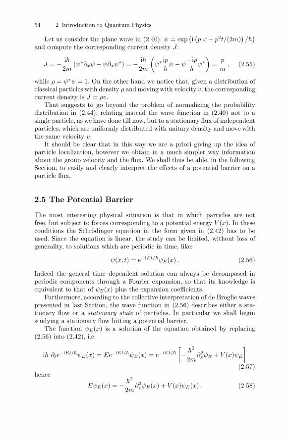
54 2 Introduction to Quantum Physics
Let us consider the plane wave in (2.40): ψ = exp(i(p x− p2t/(2m)
)/h)
and compute the corresponding current density J :
J = − ih
2m(ψ∗∂xψ − ψ∂xψ∗) = − ih
2m
(ψ∗
ip
hψ − ψ
−ip
hψ∗)
=p
m, (2.55)
while ρ = ψ∗ψ = 1. On the other hand we notice that, given a distribution ofclassical particles with density ρ and moving with velocity v, the correspondingcurrent density is J = ρv.
That suggests to go beyond the problem of normalizing the probabilitydistribution in (2.44), relating instead the wave function in (2.40) not to asingle particle, as we have done till now, but to a stationary flux of independentparticles, which are uniformly distributed with unitary density and move withthe same velocity v.
It should be clear that in this way we are a priori giving up the idea ofparticle localization, however we obtain in a much simpler way informationabout the group velocity and the flux. We shall thus be able, in the followingSection, to easily and clearly interpret the effects of a potential barrier on aparticle flux.
2.5 The Potential Barrier
The most interesting physical situation is that in which particles are notfree, but subject to forces corresponding to a potential energy V (x). In theseconditions the Schrodinger equation in the form given in (2.42) has to beused. Since the equation is linear, the study can be limited, without loss ofgenerality, to solutions which are periodic in time, like:
ψ(x, t) = e−iEt/hψE(x) . (2.56)
Indeed the general time dependent solution can always be decomposed inperiodic components through a Fourier expansion, so that its knowledge isequivalent to that of ψE(x) plus the expansion coefficients.
Furthermore, according to the collective interpretation of de Broglie wavespresented in last Section, the wave function in (2.56) describes either a sta-tionary flow or a stationary state of particles. In particular we shall beginstudying a stationary flow hitting a potential barrier.
The function ψE(x) is a solution of the equation obtained by replacing(2.56) into (2.42), i.e.
ih ∂te−iEt/hψE(x) = Ee−iEt/hψE(x) = e−iEt/h
[− h2
2m∂2
xψE + V (x)ψE
](2.57)
hence
EψE(x) = − h2
2m∂2
xψE(x) + V (x)ψE(x) , (2.58)
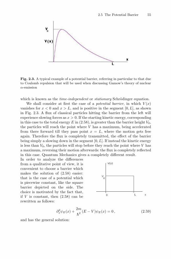
2.5 The Potential Barrier 55
Fig. 2.3. A typical example of a potential barrier, referring in particular to that dueto Coulomb repulsion that will be used when discussing Gamow’s theory of nuclearα-emission
which is known as the time-independent or stationary Schrodinger equation.We shall consider at first the case of a potential barrier, in which V (x)
vanishes for x < 0 and x > L, and is positive in the segment [0, L], as shownin Fig. 2.3. A flux of classical particles hitting the barrier from the left willexperience slowing forces as x > 0. If the starting kinetic energy, correspondingin this case to the total energy E in (2.58), is greater than the barrier height V0,the particles will reach the point where V has a maximum, being acceleratedfrom there forward till they pass point x = L, where the motion gets freeagain. Therefore the flux is completely transmitted, the effect of the barrierbeing simply a slowing down in the segment [0, L]. If instead the kinetic energyis less than V0, the particles will stop before they reach the point where V hasa maximum, reversing their motion afterwards: the flux is completely reflectedin this case. Quantum Mechanics gives a completely different result.In order to analyze the differencesfrom a qualitative point of view, it isconvenient to choose a barrier whichmakes the solution of (2.58) easier:that is the case of a potential whichis piecewise constant, like the squarebarrier depicted on the side. Thechoice is motivated by the fact that,if V is constant, then (2.58) can berewritten as follows:
∂2xψE(x) +
2m
h2 (E − V )ψE(x) = 0 , (2.59)
and has the general solution:

56 2 Introduction to Quantum Physics
ψE(x) = a+ exp
(i
√2m(E − V )
hx
)+ a− exp
(−i
√2m(E − V )
hx
), (2.60)
if E > V , while
ψE(x) = a+ exp
(√2m(V − E)
hx
)+ a− exp
(−√
2m(V − E)
hx
), (2.61)
in the opposite case. The problem is then to establish how the solution foundin a definite region can be connected to those found in the nearby regions.In order to solve this kind of problem we must be able to manage differentialequations in presence of discontinuities in their coefficients, and that requiresa brief mathematical interlude.
2.5.1 Mathematical Interlude: Differential Equations
with Discontinuous Coefficients
Differential equations with discontinuous coefficients can be treated by smooth-ing the discontinuities, then solving the equations in terms of functions whichare derivable several times, and finally reproducing the correct solutions inpresence of discontinuities through a limit process. In order to do so, let usintroduce the function ϕε(x), which is defined as
ϕε(x) = 0 if |x| > ε ,
ϕε(x) =ε2 + x2
2 (ε2 − x2)2
1
cosh2 (x/(ε2 − x2))if |x| < ε .
This function, as well as all of its derivatives, is continuous and it can be easilyshown that
∫ ∞
−∞ϕε(x)dx = 1 .
Based on this property we conclude that if f(x) is locally integrable, i.e. if itadmits at most isolated singularities where the function may diverge with adegree less than one, like for instance 1/|x|1−δ when δ > 0, then the integral∫ ∞
−∞ϕε(x− y)f(y)dy ≡ fε(x)
defines a function which can be derived in x an infinite number of times; thederivatives of fε tend to those of f in the limit ε → 0 and in all points wherethe latter are defined. We have in particular, by part integration,

2.5 The Potential Barrier 57
dn
dxnfε(x) =
∫ ∞
−∞ϕε(x− y)
dn
dynf(y)dy ; (2.62)
fε is called regularized function. If for in-stance we consider the case in which f isthe step function in the origin, i.e. f(x) = 0for x < 0 and f(x) = 1 for x > 0,we have for fε(x), ∂xfε(x) = f ′ε(x) and∂2
xfε(x) = f ′′ε (x) the behaviours showed inthe respective order on the side. Notice inparticular that since
fε(x) =
∫ ∞
0
ϕε(x− y)dy =
∫ x
−∞ϕε(z)dz
we have ∂xfε(x) = ϕε(x). By looking atthe three figures it is clear that fε(x) con-tinuously interpolates between the two val-ues, zero and one, which the function as-sumes respectively to the left of −ε and tothe right of ε, staying less than 1 for everyvalue of x. It is important to notice that in-stead the second figure, showing ∂xfε(x),i.e. ϕε(x), has a maximum of height pro-portional to 1/ε2, hence diverging as ε → 0.
The third figure, showing the secondderivative ∂2
xfε(x), has an oscillation ofamplitude proportional to 1/ε4 around thediscontinuity point. Since, for small ε, theregularized function depends, close to thediscontinuity, on the nearby values of theoriginal function, it is clear that the qual-itative behaviors showed in the figures arevalid, close to discontinuities of the firstkind (i.e. where the function itself has adiscontinuous gap), for every starting func-tion f .
Let us now consider (2.59) close to a discontinuity point of the first kind(step function) for V , and suppose we regularize both terms on the left handside. Assuming that the wave function do not present discontinuities worsethan first kind, the second term in the equation may present only steps so that,once regularized, it is limited independently of ε. However the first term maypresent oscillations of amplitude ∼ 1/ε4 if ψE has a first kind discontinuity, ora peak of height ∼ ±1/ε2 if ψE is continuous but its first derivative has suchdiscontinuity: in each case the modulus of the first regularized term would

58 2 Introduction to Quantum Physics
diverge faster than the second in the limit ε → 0. That shows that in presenceof a first kind discontinuity in V , both the wave function ψE and its derivativemust be continuous.
In order to simply deal with barriers of length L much smaller than thetypical wavelengths of the problem, it is useful to introduce infinitely thin bar-riers: that can be done by choosing a potential energy which, once regularized,is equal to Vε(x) = V ϕε(x), i.e.
V (x) = V limε→0
ϕε(x) ≡ Vδ(x) . (2.63)
Equation (2.63) defines the so-called Dirac’s delta function as a limit of ϕε.When studying Schrodinger equation regularized as done above, it is pos-
sible to show, by integrating the differential equation between −ε and ε, thatin presence of a potential barrier proportional to the Dirac delta function thewave function stays continuous, but its derivative has a first kind discontinuityof amplitude
limε→0
(ψ′E(ε)− ψ′E(−ε)) =2m
h2 VψE(0) . (2.64)
Notice that a potential barrier proportional to the Dirac delta function canbe represented equally well by a square barrier of height V/L and width L, inthe limit as L → 0 with
∫∞−∞ dxV (x) = V kept constant.
2.5.2 The Square Barrier
Let us consider the stationary Schrodinger equation (2.58) with a potentialcorresponding to the square barrier described above, that is V (x) = V for0 < x < L and vanishing elsewhere. As in the classical case we can distinguishtwo different regimes:a) the case E > V , in which classically the flux would be entirely transmitted;b) the opposite case, E < V , in which classically the flux would be entirelyreflected.Let us start with case (a) and distinguish three different regions:1) the region x < 0, in which the general solution is
ψE(x) = a+ei√
2mE x/h + a−e−i√
2mE x/h ; (2.65)
this wave function corresponds to two opposite fluxes, the first moving right-wards and equal to |a+|2
√2E/m, the other opposite to the first and equal to
−|a−|2√
2E/m. Since we want to study a quantum process analogous to thatdescribed classically, we arbitrarily choose a+ = 1, thus fixing the incidentflux to
√2E/m, hence
ψE(x) = ei√
2mE x/h + a e−i√
2mE x/h ; (2.66)
a takes into account the possible reflected flux, |a|2√2E/m. The physicallyinteresting quantity is the fraction of the incident flux which is reflected, which

2.5 The Potential Barrier 59
is called the reflection coefficient of the barrier and, with our normalizationfor the incident flux, is R = |a|2;2) the region 0 < x < L, where the general solution is
ψE(x) = b ei√
2m(E−V ) x/h + c e−i√
2m(E−V ) x/h ; (2.67)
3) the region x > L, where the general solution is given again by (2.65).However, since we want to study reflection and transmission through the bar-rier, we exclude the possibility of a backward flux, i.e. coming from x = ∞,thus assuming that the only particles present in this region are those goingrightwards after crossing the barrier. Therefore in this region we write
ψE(x) = d ei√
2mE x/h . (2.68)
The potential has two discontinuities in x = 0 and x = L, therefore wehave the following conditions for the continuity of the wave function and itsderivative:
1 + a = b + c ,
1− a =
√E − V
E(b− c) ,
b ei√
2m(E−V )L/h + c e−i√
2m(E−V )L/h = d ei√
2mEL/h , (2.69)√E − V
E
[b ei√
2m(E−V )L/h − c e−i√
2m(E−V )L/h]
= d ei√
2mEL/h .
We have thus a linear system of 4 equations with 4 unknown variables which,for a generic choice of parameters, should univocally identify the solution.However our main interest is the determination of |a|2. Dividing side by sidethe first two as well as the last two equations, we obtain after simple algebra:
1− a
1 + a=
√E − V
E
bc − 1bc + 1
,
bc − e−2i
√2m(E−V )L/h
bc + e−2i
√2m(E−V )L/h
=
√E
E − V. (2.70)
Solving the second equation for b/c and the first for a we obtain:
b
c= e−2i
√2m(E−V )L/h
√E−V
E + 1√E−V
E − 1,
a =1 +
√E−V
E + bc
(1−
√E−V
E
)1−
√E−V
E + bc
(1 +
√E−V
E
) (2.71)

60 2 Introduction to Quantum Physics
and finally, by substitution:
a =
(1− E−V
E
) (ei√
2m(E−V )L/h − e−i√
2m(E−V )L/h)
(1−
√E−V
E
)2
ei√
2m(E−V )L/h −(1 +
√E−V
E
)2
e−i√
2m(E−V )L/h
,
so that
a =V
E
sin
(√(2m(E−V )
h L
)2E−V
E sin
(√(2m(E−V )
h L
)+ 2i
√E−V
E cos
(√(2m(E−V )
h L
) , (2.72)
which clearly shows that 0 ≤ |a| < 1 and that, for V > 0, a vanishes onlywhen
√(2m(E − V )L/h = nπ.
This is a clear interference effect, showing that reflection by the barrier isa wavelike phenomenon. For those knowing the physics of coaxial cables thereshould be a clear analogy between our result and the reflection happeningat the junction of two cables having mismatching impedances: television settechnicians well known that as a possible origin of failure.
The quantum behavior in case (b), i.e. when E < V , is more interestingand important for its application to microscopic physics. In this case the wavefunctions in regions 1 and 3 do not change, while for 0 < x < L the generalsolution is:
ψE(x) = b e√
2m(V−E) x/h + c e−√
2m(V−E) x/h , (2.73)
so that the continuity conditions become:
1 + a = b + c ,
1− a = −i
√V − E
E(b− c) ,
b e√
2m(V−E)L/h + c e−√
2m(V−E)L/h = d ei√
2mEL/h , (2.74)
−i
√V − E
E
[b e√
2m(V−E)L/h − c e−√
2m(V−E)L/h]
= d ei√
2mEL/h .
Dividing again side by side we have:
bc − e−2
√2m(V−E)L/h
bc + e−2
√2m(V−E)L/h
= i
√E
V − E,
1− a
1 + a= i
√V − E
E
1− bc
1 + bc
, (2.75)

2.5 The Potential Barrier 61
which can be solved as follows:
a = −1− b
c + i√
EV−E
(1 + b
c
)1− b
c − i√
EV−E
(1 + b
c
) ,
b
c= e−2
√2m(V−E)L/h
1 + i√
EV−E
1− i√
EV−E
. (2.76)
We can get the expression for a, hence the reflection coefficient R ≡ |a|2, byreplacing b/c in the first equation. The novelty is that R is not equal to onesince, as it is clear from (2.76), b/c is a complex number. Therefore a fraction1 −R ≡ T of the incident flux is transmitted through the barrier, in spite ofthe fact that, classically, the particles do not have enough energy to reach thetop of it. That is known as tunnel effect and plays a very important role inseveral branches of modern physics, from radioactivity to electronics.
Instead of giving a complete solution for a, hence for the transmission
coefficient T , and in order to avoid too complex and unreadable formulae, wewill confine the discussion to two extreme cases, which however have a greatphenomenological interest. We consider in particular:
a) the case in which e−2√
2m(V−E)L/h � 1, with a generic value for EV−E , i.e.
L � h/√
2m(V − E), which is known as the thick barrier case;b) the case in which the barrier is thin, corresponding in particular to thelimit L → 0 with V L ≡ V kept constant.
The thick barrier
In this case |b/c| is small, so that it could be neglected in a first approximation,however it is clear from (2.76) that if b/c = 0 then |a| = 1, so that thereis actually no tunnel effect. For this reason we must compute the Taylorexpansion in the expression of a as a function of b/c up to the first order:
a = −1 + i
√E
V−E
1− i√
EV−E
1− bc
1−i√
E/(V−E)
1+i√
E/(V−E)
1− bc
1+i√
E/(V−E)
1−i√
E/(V−E)
∼ −1 + i
√E
V−E
1− i√
EV−E
⎡⎣1− b
c
⎛⎝1− i
√E
V−E
1 + i√
EV−E
−1 + i
√E
V−E
1− i√
EV−E
⎞⎠⎤⎦
= −1 + i
√E
V−E
1− i√
EV−E
[1 + 4i
b
c
√E(V − E)
V
](2.77)
= −1 + i
√E
V−E
1− i√
EV−E
⎡⎣1 + 4i
√E(V − E)
Ve−2√
2m(V−E)L/h1 + i
√E
V−E
1− i√
EV−E
⎤⎦ .

62 2 Introduction to Quantum Physics
In the last line we have replaced b/c by the corresponding expression in (2.76).
Neglecting terms of the order of e−4√
2m(V−E)L/h or smaller we obtain
|a|2 = R = 1− 16E(V − E)
V 2e−2√
2m(V−E)L/h . (2.78)
Therefore the transmission coefficient, which measures the probability for aparticle hitting the barrier to cross it, is given by:
T ≡ 1−R = 16E(V − E)
V 2e−2√
2m(V−E)L/h . (2.79)
Notice that the result seems to vanish for V = E, but this is not true since inthis case the terms neglected in our approximation come into play.
This formula was first applied in nuclear physics, and more precisely tostudy α emission, a phenomenon in which a heavy nucleus breaks up into alighter nucleus plus a particle carrying twice the charge of the proton androughly four times its mass, which is known as α particle. The decay can besimply described in terms of particles of mass∼ 0.66 10−26 Kg and energy E �4− 8 MeV � 10−12 J, hitting barriers of width roughly equal to 3 10−14 m;the difference V − E is of the order of 10 MeV � 1.6 10−12 J.
In these conditions we have 2√
2m(V − E)L /h � 83 and therefore T ∼e−2√
2m(V−E)L/h ∼ 10−36. Given the order of magnitude of the energy E andof the mass of the particle, we infer that it moves with a velocity of the order of107 m/s: since the radius R0 of heavy nuclei is roughly 10−14 m, the frequencyof collisions against the barrier is νu ∼ 1021 Hz. That indicates that, onaverage, the time needed for the α particle to escape the nucleus is of the orderof 1/(νuT ), i.e. about 1015 s, equal to 108 years. However, if the width of thebarrier is only 4 times smaller, the decay time goes down to about 100 years.That shows a great sensitivity of the result to the parameters and justifiesthe fact that we have neglected the pre-factor in front of the exponential in(2.79). On the other hand that also shows that, for a serious comparison withthe actual mean lives of nuclei, an accurate analysis of parameters is needed,but it is also necessary to take into account the fact that we are not dealingwith a true square barrier, since the repulsion between the nucleus and theα particle is determined by Coulomb forces, i.e. V (x) = 2Ze2/(4πε0x) for xgreater than a given threshold, see Fig. 2.3.
As a consequence, the order of magnitude of the transmission coefficientgiven in (2.79), i.e.
T � e−2√
2m(V−E)L/h (2.80)
must be replaced by1
T � exp
(−2
∫ R1
R0
dx
√2m(V (x)− E)
h
)≡ e−G , (2.81)
1 One can think of a thick, but not square, barrier as a series of thick square barriersof different heights.
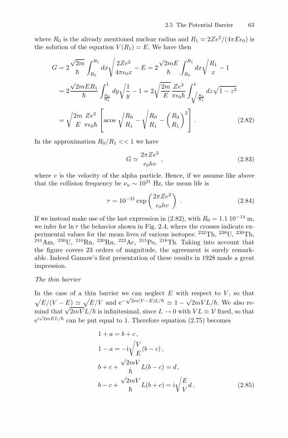
2.5 The Potential Barrier 63
where R0 is the already mentioned nuclear radius and R1 = 2Ze2/(4πEε0) isthe solution of the equation V (R1) = E. We have then
G = 2
√2m
h
∫ R1
R0
dx
√2Ze2
4πε0x− E = 2
√2mE
h
∫ R1
R0
dx
√R1
x− 1
= 2
√2mER1
h
∫ 1
R0R1
dy
√1
y− 1 = 2
√2m
E
Ze2
πε0h
∫ 1√R0R1
dz√
1− z2
=
√2m
E
Ze2
πε0h
⎡⎣acos
√R0
R1−√
R0
R1−(
R0
R1
)2⎤⎦ . (2.82)
In the approximation R0/R1 << 1 we have
G � 2πZe2
ε0hv, (2.83)
where v is the velocity of the alpha particle. Hence, if we assume like abovethat the collision frequency be νu ∼ 1021 Hz, the mean life is
τ = 10−21 exp
(2πZe2
ε0hv
). (2.84)
If we instead make use of the last expression in (2.82), with R0 = 1.1 10−14 m,we infer for ln τ the behavior shown in Fig. 2.4, where the crosses indicate ex-perimental values for the mean lives of various isotopes: 232Th, 238U, 230Th,241Am, 230U, 210Rn, 220Rn, 222Ac, 215Po, 218Th. Taking into account thatthe figure covers 23 orders of magnitude, the agreement is surely remark-able. Indeed Gamow’s first presentation of these results in 1928 made a greatimpression.
The thin barrier
In the case of a thin barrier we can neglect E with respect to V , so that√E/(V − E) � √
E/V and e−√
2m(V−E)L/h � 1 − √2mV L/h. We also re-
mind that√
2mV L/h is infinitesimal, since L → 0 with V L ≡ V fixed, so that
ei√
2mEL/h can be put equal to 1. Therefore equation (2.75) becomes
1 + a = b + c ,
1− a = −i
√V
E(b− c) ,
b + c +
√2mV
hL(b− c) = d ,
b− c +
√2mV
hL(b + c) = i
√E
Vd , (2.85)

64 2 Introduction to Quantum Physics
Fig. 2.4. The mean lives of a sample of α-emitting isotopes plotted against thecorresponding α-energies. The solid line shows the values predicted by Gamow’stheory
and substituting b± c we obtain:
d = 1 + a + i
√E
V
√2mV
hL(1− a) � 1 + a ,
i
√E
V(1− a) +
√2mV
hL(1 + a) = i
√E
Vd , (2.86)
in its simplest form. Taking further into account our approximation, the sys-tem can be rewritten as
1 + a = d ,
1− a =
(i
√2m
E
V L
h+ 1
)d ≡
(1 + i
√2m
E
Vh
)d . (2.87)
Finally we find, by eliminating a, that
d =1
1 + i√
m2E
Vh
, (2.88)
hence
T =1
1 + m2E
V2
h2
(2.89)
and
R =1
1 + 2Em
h2
V2
. (2.90)

2.6 Quantum Wells and Energy Levels 65
Notice that the system (2.87) confirms what predicted about the continuityconditions for the wave function in presence of a potential energy equal toVδ(x), i.e. that the wave function is continuous (1+a = d) while its derivativehas a discontinuity (i
√2mE(1 − a − d)/h) equal to 2mV/h2 times the value
of the wave function (d in our case).
2.6 Quantum Wells and Energy Levels
Having explored the tunnel effect in some details, let us now discuss the solu-tions of the Schrodinger equation in the case of binding potentials. For boundstates, i.e. for solutions with wave functions localized in the neighborhood ofa potential well, we expect computations to lead to energy quantization, i.e.to the presence of discrete energy levels. Let us start our discussion from thecase of a square well
V (x) = −V for |x| < L
2, V (x) = 0 for |x| > L
2. (2.91)
Notice that the origin of the co-ordinate has been chosen in or-der to emphasize the symme-
try of the system, correspond-ing in this case to the invari-ance of Schrodinger equationunder axis reflection x → −x.In general the symmetry of thepotential allows us to find newsolutions of the equation starting from known solutions, or to simplify thesearch for solutions by a priori fixing some of their features. In this case itcan be noticed that if ψE(x) is a solution, ψE(−x) is a solution too, so that,by linearity of the differential equation, any linear combination (with complexcoefficients) of the two wave functions is a good solution corresponding to thesame value of the energy E, in particular the combinations ψE(x)± ψE(−x),which are even/odd under reflection of the x axis. Naturally one of the twosolutions may well vanish, but it is clear that all possible solutions can bedescribed in terms of (i.e. they can be written as linear combinations of)functions which are either even or odd under x-reflection.
To better clarify the point, let us notice that, since the Schrodinger equa-tion is linear, the set of all its possible solutions having the same energyconstitutes what is usually called a linear space, which is completely fixedonce we know one particular basis for it. What we have learned is that inthe present case even/odd functions are a good basis, so that the search forsolutions can be solely limited to them. This is probably the simplest exampleof the application of a symmetry principle asserting that, if the Schrodingerequation is invariant under a coordinate transformation, it is always possible

66 2 Introduction to Quantum Physics
to choose its solutions so that the transformation does not change them butfor a constant phase factor, which in the present case is ±1.
We will consider in the following only bound solutions which, assumingthat the potential energy vanishes as |x| → ∞, correspond to a negative totalenergy E and are therefore the analogous of bound states in classical mechan-ics. Solutions with positive energy instead present reflection and transmissionphenomena, as in the case of barriers. We notice that, in the case of boundstates, the collective interpretation of the wave function does not apply, sincethese are states involving a single particle: that is in strict relation with thefact that bound state solutions vanish rapidly enough as |x| → ∞, so that theprobability distribution in (2.44) can be properly normalized.
Let us start by considering even solutions: it is clear that we can limitour study to the positive x axis, with the additional constraint of a vanishingfirst derivative in the origin, as due for an even function (whose derivative isodd). We can divide the positive x axis into two regions where the potentialis constant:a) that corresponding to x < L/2, where the general solution is:
ψE(x) = a+ei√
2m(E+V ) x/h + a−e−i√
2m(E+V ) x/h ,
which is even for a+ = a−, so that
ψE(x) = a cos
(√2m(E + V )
hx
); (2.92)
b) that corresponding to x > L/2, where the general solution is:
ψE(x) = b+e√
2m|E| x/h + b−e−√
2m|E| x/h .
The condition that |ψ|2 be an integrable function constrains b+ = 0, otherwisethe probability density would unphysically diverge as |x| → ∞; therefore wecan write
ψE(x) = b e−√
2m|E| x/h . (2.93)
Notice that we have implicitly excluded the possibility E < −V , the reasonbeing that in this case (2.92) would be replaced by
ψE(x) = a cosh
(√2m|E + V |
hx
)
which for x > 0 has a positive logarithmic derivative (∂xψE(x)/ψE(x)) whichcannot continuously match the negative logarithmic derivative of the solutionin the second region given in (2.93). Therefore quantum theory is in agreementwith classical mechanics about the impossibility of having states with totalenergy less than the minimum of the potential energy.

2.6 Quantum Wells and Energy Levels 67
The solutions of the Schrodinger equation on the whole axis can be foundby solving the system:
a cos
√2m(E + V )L
2h= b e−
√2m|E|L/(2h) ,√
2m(E + V )
ha sin
√2m(E + V )L
2h=
√2m|E|h
b e−√
2m|E|L/(2h) (2.94)
dividing previous equations side by side we obtain the continuity conditionfor the logarithmic derivative:
tan
√2m(E + V )L
2h=
√|E|
E + V. (2.95)
In order to discuss last equation let us introduce the variable
x ≡√
2m(E + V )L
2h(2.96)
and the parameter
y ≡√
2mV L/2h , (2.97)
and let us plot together the behav-ior of the two functions tanx and√
(y2 − x2)/x2 =√|E|/(E + V ). In
the figure we show the case y2 = 20.From a qualitative point of view thefigure shows that energy levels, corre-sponding to the intersection points ofthe two functions, are quantized, thusconfirming also for the case of po-tential wells the discrete energy spec-trum predicted by Bohr’s theory. Inparticular the plot shows two inter-sections, the first for x = x1 < π/2,the second for π < x = x2 < 3π/2.
Notice that quantization of energy derives from the physical requirementof having a bound state solution which does not diverge but instead vanishesoutside the well: for this reason the external solution is parametrized in termsof only one parameter. The reduced number of available parameters allowsfor non-trivial solutions of the homogeneous linear system (2.94) only if theenergy quantization condition (2.95) is satisfied.
The number of possible solutions increases as y grows and since y > 0it is anyway greater than zero. Therefore the square potential well in onedimension has always at least one bound state corresponding to an even wavefunction. It can be proved that the same is true for every symmetric wellin one dimension (i.e. such that V (−x) = V (x) ≤ 0). On the contrary, an
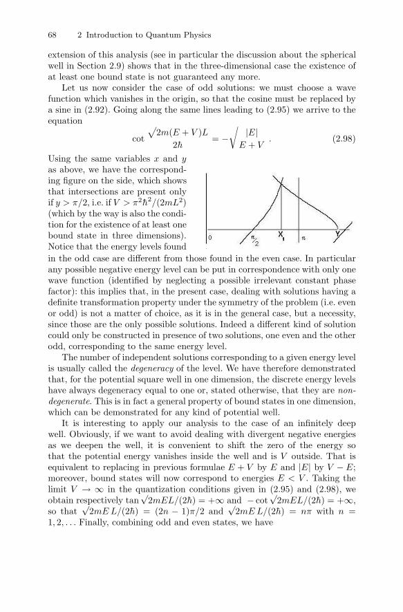
68 2 Introduction to Quantum Physics
extension of this analysis (see in particular the discussion about the sphericalwell in Section 2.9) shows that in the three-dimensional case the existence ofat least one bound state is not guaranteed any more.
Let us now consider the case of odd solutions: we must choose a wavefunction which vanishes in the origin, so that the cosine must be replaced bya sine in (2.92). Going along the same lines leading to (2.95) we arrive to theequation
cot
√2m(E + V )L
2h= −
√|E|
E + V. (2.98)
Using the same variables x and yas above, we have the correspond-ing figure on the side, which showsthat intersections are present onlyif y > π/2, i.e. if V > π2h2/(2mL2)(which by the way is also the condi-tion for the existence of at least onebound state in three dimensions).Notice that the energy levels found
in the odd case are different from those found in the even case. In particularany possible negative energy level can be put in correspondence with only onewave function (identified by neglecting a possible irrelevant constant phasefactor): this implies that, in the present case, dealing with solutions having adefinite transformation property under the symmetry of the problem (i.e. evenor odd) is not a matter of choice, as it is in the general case, but a necessity,since those are the only possible solutions. Indeed a different kind of solutioncould only be constructed in presence of two solutions, one even and the otherodd, corresponding to the same energy level.
The number of independent solutions corresponding to a given energy levelis usually called the degeneracy of the level. We have therefore demonstratedthat, for the potential square well in one dimension, the discrete energy levelshave always degeneracy equal to one or, stated otherwise, that they are non-
degenerate. This is in fact a general property of bound states in one dimension,which can be demonstrated for any kind of potential well.
It is interesting to apply our analysis to the case of an infinitely deepwell. Obviously, if we want to avoid dealing with divergent negative energiesas we deepen the well, it is convenient to shift the zero of the energy sothat the potential energy vanishes inside the well and is V outside. That isequivalent to replacing in previous formulae E + V by E and |E| by V − E;moreover, bound states will now correspond to energies E < V . Taking thelimit V → ∞ in the quantization conditions given in (2.95) and (2.98), weobtain respectively tan
√2mEL/(2h) = +∞ and − cot
√2mEL/(2h) = +∞,
so that√
2mE L/(2h) = (2n − 1)π/2 and√
2mE L/(2h) = nπ with n =1, 2, . . . Finally, combining odd and even states, we have

2.6 Quantum Wells and Energy Levels 69
√2mE
hL = nπ : n = 1, 2, . . .
and the following energy levels
En =n2π2h2
2mL2. (2.99)
The corresponding wave functions vanish outside the well while in the region|x| < L/2 the even functions are
√2/L cos (2n− 1)πx/L and the odd ones
are√
2/L sin 2nπx/L, with the coefficients fixed in order to satisfy (2.44). Itis also possible to describe all wave functions by a unique formula:
ψEn(x) =
√2
Lsin
nπ(x + L2 )
Lfor |x| < L
2,
ψEn(x) = 0 for |x| > L
2. (2.100)
While all wave functions are contin-uos in |x| = L/2, their derivatives arenot, as in the case of the potentialbarrier proportional to the Dirac deltafunction. The generic solution ψEn
hasthe behaviour showed in the figure,where the analogy with the electriccomponent of an electromagnetic wavereflected between two mirrors clearlyappears. Therefore the infinitely deepwell can be identified as the region be-tween two reflecting walls.
If the wave amplitude vanishes over the mirrors, the distance betweenthem must necessarily be an integer multiple of half the wavelength; this isthe typical tuning condition for a musical instrument and implies wavelengthand energy quantization. The exact result agrees with that of Problem 2.4.
Going back to the analogy with electromagnetic waves, the present situa-tion corresponds to a one-dimensional resonant cavity. In the cavity the fieldcan only oscillate according to the permitted wavelengths, which are λn =2L/n for n = 1, 2, . . . corresponding to the frequencies νn = c/λn = nc/(2L),which are all multiple of the fundamental frequency of the cavity.
Our results regarding the infinitely deep well can be easily generalized tothree dimensions. To that purpose, let us introduce a cubic box of side L withreflecting walls. The condition that the wave function vanishes over the wallsis equivalent, inside the box and choosing solutions for which the dependenceon x,y and z is factorized, to:
70 2 Introduction to Quantum Physics
ψnx,ny,nz=
√8
L3sin
nxπ(x + L2 )
Lsin
nyπ(y + L2 )
Lsin
nzπ(z + L2 )
L, (2.101)
where we have assumed the origin of the coordinates to be placed in the centerof the box. The corresponding energy coincides with the kinetic energy insidethe box and can be obtained by writing the Schrodinger equation in threedimensions:
− h2
2m
(∂2
x + ∂2y + ∂2
z
)ψnx,ny,nz
= Enx,ny,nzψnx,ny,nz
, (2.102)
leading to
Enx,ny,nz=
π2h2
2mL2
[n2
x + n2y + n2
z
]. (2.103)
This result will be useful for studying the properties of a gas of non-interactingparticles (perfect gas) contained in a box with reflecting walls. Following thesame analogy as above one can study in a similar way the oscillations of anelectromagnetic field in a three-dimensional cavity, with proper frequencies
given by νnx,ny,nz= (c/2L)
√n2
x + n2y + n2
z.
2.7 The Harmonic Oscillator
The one-dimensional harmonic oscillator can be identified with the mechanicalsystem formed by a particle of mass m bound to a fixed point (taken as theorigin of the coordinate) by an ideal spring of elastic constant k and vanishinglength at rest. This is equivalent to a potential energy V (x) = kx2/2. Inclassical mechanics the corresponding equation of motion is
mx + kx = 0 ,
whose general solution is
x(t) = X cos(ωt + φ) ,
where ω =√
k/m = 2πν and ν is the proper frequency of the oscillator.At the quantum level we must solve the following stationary Schrodinger
equation:
− h2
2m∂2
xψE(x) +mω2
2x2ψE(x) = EψE(x) . (2.104)
In order to solve this equation we can use the identity(√mω2
2x− h√
2m∂x
)(√mω2
2x +
h√2m
∂x
)f(x)
≡ mω2
2x2f(x) +
hω
2x∂xf(x) − hω
2∂x(xf(x)) − h2
2m∂2
xf(x)

2.7 The Harmonic Oscillator 71
= − h2
2m∂2
xf(x) +mω2
2x2f(x)− hω
2f(x)
≡(− h2
2m∂2
x +mω2
2x2 − hω
2
)f(x) , (2.105)
which is true for any function f which is derivable at least two times.It is important to notice the operator notation used in last equation, where
we have introduced some specific symbols, (√
mω2/2 x ± (h/√
2m) ∂x) or
(−(h2/2m) ∂2x + (mω2/2) x2 − hω/2), to indicate operations in which deriva-
tion and multiplication by some variable are combined together. These areusually called operators, meaning that they give a correspondence law be-tween functions belonging to some given class (for instance those which canbe derived n times) and other functions belonging, in general, to a differentclass.
In this way, leaving aside the specific function f , equation (2.105) can berewritten as an operator relation(√
mω2
2x− h√
2m∂x
)(√mω2
2x +
h√2m
∂x
)=
(− h2
2m∂2
x +mω2
2x2 − hω
2
)(2.106)
and equations of similar nature can be introduced, like for instance:(√mω2
2x +
h√2m
∂x
)(√mω2
2x− h√
2m∂x
)
−(√
mω2
2x− h√
2m∂x
)(√mω2
2x +
h√2m
∂x
)= hω . (2.107)
In order to shorten formulae, it is useful to introduce the two symbols:
X± ≡(√
mω2
2x± h√
2m∂x
)=
√hω
2
(αx± 1
α
∂
∂x
)(2.108)
in which the constant α ≡ √mω/h has be defined, corresponding to the
inverse of the typical length scale of the system. That allows us to rewrite(2.107) in the simpler form:
X+X− −X−X+ = hω . (2.109)
If, extending the operator formalism, we define
H ≡ − h2
2m∂2
x +mω2
2x2 , (2.110)
we can rewrite (2.106) as:
72 2 Introduction to Quantum Physics
X−X+ = H − hω
2, (2.111)
then obtaining from (2.109):
X+X− = H +hω
2. (2.112)
The Schrodinger equation can be finally written as:
HψE(x) = EψE(x) . (2.113)
The operator formalism permits to get quite rapidly a series of results.a) The wave function which is solution of the equation
X+ψ0(x) =
√mω2
2xψ0(x) +
h√2m
∂xψ0(x) = 0 , (2.114)
is also a solution of (2.113) with E = hω/2. In order to compute it we canrewrite (2.114) as:
∂xψ0(x)
ψ0(x)= −α2x ,
hence, integrating both members:
ln ψ0(x) = c− α2
2x2 ,
from which it follows that
ψ0(x) = ec e−α2x2/2 ,
where the constant c can be fixed by the normalization condition given in(2.44), leading finally to
ψ0(x) =(mω
πh
) 14
e−mωx2/(2h) . (2.115)
We would like to remind the need for restricting the analysis to the so-calledsquare integrable functions, which can be normalized according to (2.44). Thisis understood in the following.
b) What we have found is the lowest energy solution, usually called theground state of the system, as can be proved by observing that, for everynormalized solution ψE(x), the following relations hold:
∫ ∞
−∞dxψE(x)∗
(√mω2
2x− h√
2m∂x
)(√mω2
2x +
h√2m
∂x
)ψE(x)
=
∫ ∞
−∞dx|X+ψE(x)|2 =
∫ ∞
−∞dxψE(x)∗
(E − hω
2
)ψE(x)
= E − hω
2≥ 0 , (2.116)

2.7 The Harmonic Oscillator 73
where the derivative in X− has been integrated by parts, exploiting the van-ishing of the wave function at x = ±∞. Last inequality follows from the factthat the integral of the squared modulus of any function cannot be negative.Moreover it must be noticed that if the integral vanishes, i.e. if E = hω/2,then necessarily X+ψE = 0, so that ψE is proportional to ψ0. That provesthat the ground state is unique.
c) If ψE satisfies (2.104) then X±ψE satisfies the same equation with Ereplaced by E ∓ hω, i.e. we have
HX±ψE = (E ∓ hω)X±ψE . (2.117)
Notice that X+ψE vanishes if and only if ψE = ψ0 while X−ψE never vanishes:one can prove this by verifying that if X−ψE = 0 then ψE behaves as ψ0 butwith the sign + in the exponent, hence it is not square integrable. In order toprove equation (2.117), from (2.111) and (2.112) we infer, for instance:
X+X−X+ψE = X+
(H − hω
2
)ψE(x) =
(H +
hω
2
)X+ψE(x)
= X+
(E − hω
2
)ψE(x) =
(E − hω
2
)X+ψE(x) (2.118)
from which (2.117) follows in the + case.Last computations show that operators combine in a fashion which resem-
bles usual multiplication, however their product is strictly dependent on theorder in which they appear. We say that the product is non-commutative;that is also evident from (2.109), which expresses what is usually known asthe commutator of two operators.
Exchanging X− and X+ in previous equations we have:
X−X+X−ψE = X−
(H +
hω
2
)ψE(x) =
(H − hω
2
)X−ψE(x)
= X−
(E +
hω
2
)ψE(x) =
(E +
hω
2
)X−ψE(x) (2.119)
which completes the proof of (2.117).d) Finally, combining points (a–c), we can show that the only possible
energy levels are:
En =
(n +
1
2
)hω . (2.120)
In order to prove that, let us suppose instead that (2.104) admits the levelE = (m + 1/2) hω + δ, where 0 < δ < hω, and then repeatedly apply X+ toψE up to m+1 times. If Xk
+ψE = 0 with k ≤ m+1 and Xk−1+ ψE = 0, then we
would have X+(Xk−1+ ψE) = 0 which, as we have already seen, is equivalent
to Xk−1+ ψE ∼ ψ0, hence to HXk−1
+ ψE = hω/2ψE . However equation (2.117)
implies HXk−1+ ψE = (E − (k− 1)hω)ψE , hence E = (k− 1/2)hω, which is in

74 2 Introduction to Quantum Physics
contrast with the starting hypothesis (δ = 0). On the other hand Xk+ψE = 0
even for k = m + 1 would imply the presence of a solution with energy lessthat hω/2, in contrast with (2.116). We have instead no contradiction if δ = 0and k = m + 1.
We have therefore shown that the spectrum of the harmonic oscillatorconsists of the energy levels En = (n + 1/2) hω. We also know from (2.117)that ∼ Xn
−ψ0 is a possible solution with E = En: we will now show that thisis actually the only possible solution.
e) Any wave function corresponding to the n-th energy level is necessarilyproportional to Xn−ψ0:
ψEn∼ Xn
−ψ0 . (2.121)
We already know that this is true for n = 0 (ground state). Now let us supposethe same to be true for n = k and we shall prove it for n = k + 1, thusconcluding our argument by induction. Let ψEk+1
be a solution correspondingto Ek+1, then, by (2.117) and by the uniqueness of ψEk
, we have
X+ψEk+1= aψEk
(2.122)
for some constant a = 0, with ψEk∝ Xk
−ψ0. By applying X− to both sides oflast equation we obtain
X−X+ψEk+1=
(H − hω
2
)ψEk+1
= (k + 1) hω ψEk+1
= X−aψEk∝ X−Xk
−ψ0 = Xk+1− ψ0 , (2.123)
which proves that also ψEk+1is proportional to Xk+1
− ψ0.In order to find the correct normalization factor, let us first find it for
ψEk+1, assuming that ψEk
is already correctly normalized. We notice that∫ ∞
−∞dx |X−ψEk
|2 =
∫ ∞
−∞dxψ∗Ek
X+X−ψEk=
∫ ∞
−∞dxψ∗Ek
(H +
hω
2
)ψEk
= hω(k + 1)
∫ ∞
−∞dx |ψEk
|2 = hω(k + 1) , (2.124)
where in the first equality one of the X− operators has been integrated byparts and in the second equality equation (2.112) has been used. We concludethat ψEk+1
= (hω(k + 1))−1/2X−ψEk, hence, setting for simplicity ψn ≡ ψEn
:
ψn =
√1
n!
(X−√hω
)n
ψ0 ≡√
1
n!(A†)nψ0 (2.125)
where one defines A† ≡ X−/√
hω.That concludes our analysis of the one-dimensional harmonic oscillator,
which, based on an algebraic approach, has led us to finding both the pos-sible energy levels, given in (2.120), and the corresponding wave functions,

2.7 The Harmonic Oscillator 75
described by (2.115) and (2.121). In particular, confirming a general propertyof bound states in one dimension, we have found that the energy levels arenon-degenerate. The operators X+ and X− permit to transform a given so-lution into a different one, in particular by rising (X−) or lowering (X+) theenergy level by one quantum hω.
Also in this case, as for the square well, solutions have definite transforma-tion properties under axis reflection, x→ −x, which follow from the symmetryof the potential, V (−x) = V (x). In particular they are divided in even andodd functions according to the value of n, ψn(−x) = (−1)nψn(x), as can beproved by noticing that ψ0 is an even function and that the operator X−transforms an even (odd) function into an odd (even) one.
Moreover we notice that, according to (2.121), (2.115) and to the expres-sion for X− given in (2.108), all wave functions are real. This is also a generalproperty of bound states in one dimension, which can be easily proved andhas a simple interpretation. Indeed, suppose ψE be the solution of the sta-tionary Schrodinger equation (2.58) corresponding to a discrete energy levelE; since obviously both E and the potential energy V (x) are real, it follows,by taking the complex conjugate of both sides of (2.58), that also ψ∗E is agood solution corresponding to the same energy. However the non-degeneracyof bound states in one dimension implies that ψE must be unique. The onlypossibility is ψ∗E ∝ ψE , hence ψ∗E = eiφψE , so that, leaving aside an irrelevantoverall phase factor, ψE is a real function.
On the other hand, recalling the definition of the probability current den-sity J given in (2.43), it can be easily proved that the wave function is real ifand only if the current density vanishes everywhere. Since we are consideringa stationary problem, the probability density is constant in time by defini-tion and the conservation equation (2.27) implies, in one dimension, that thecurrent density J is a constant in space (the same is not true in more thanone dimension, where that translates in J being a vector field with vanishingdivergence, see Problem 2.48). On the other hand, for a bound state J mustsurely vanish as |x| → ∞, hence it must vanish everywhere, implying a realwave function: in a one-dimensional bound state there is no current flow atall.
Our results admit various generalizations of great physical interest. First ofall, let us consider their extension to the isotropic three-dimensional harmonicoscillator corresponding to the following Schrodinger equation:
− h2
2m
(∂2
x + ∂2y + ∂2
z
)ψE +
mω2
2
(x2 + y2 + z2
)ψE = E ψE , (2.126)
where ψE = ψE(x, y, z) is the three-dimensional wave function. This is thetypical example of a separable Schrodinger equation: if we look for a partic-ular class of solutions, written as the product of three functions depending

76 2 Introduction to Quantum Physics
separately on x, y and z, then equation (2.126) becomes equivalent2 to threeindependent equations for three one-dimensional oscillators along x, y and z.
Therefore we conclude that the quantized energy levels are in this case:
Enx,ny,nz= hω
(nx + ny + nz +
3
2
), (2.127)
and that the corresponding wave functions are
ψnx,ny,nz(x, y, z) = ψnx
(x)ψny(y)ψnz
(z) . (2.128)
Notice that, according to (2.127) and (2.128), in three dimensions severaldegenerate solutions can be found having the same energy, corresponding toall possible integers nx, ny, nz such that nx + ny + nz = n where n is a non-negative integer. The number of such solutions is (n + 1)(n + 2)/2.
Since we have looked for particular solutions, having the dependence onx, y and z factorized, it is natural to ask if in this way we have exhausted thepossible solutions of equation (2.126). In some sense this is not true: since theSchrodinger equation is linear, we can make linear combinations (with complexcoefficients) of the (n + 1)(n + 2)/2 degenerate solutions described above,obtaining new solutions having the same energy En = (n + 3/2)hω but notwritable, in general, as the product of three functions of x, y and z. Howeverwe have exhausted all the possible solutions in some other sense: indeed it ispossible to demonstrate that no further solution can be found beyond all thepossible linear combinations of the particular solutions in equation (2.128). Inother words, all the possibile solutions of equation (2.126), which are foundfor E = (n+3/2) hω, form a linear space of dimension (n+1)(n+2)/2, havingthe particular solutions in equation (2.128) as an orthonormal basis. We havethus found a possible complete set of solutions of equation (2.126): we shallfind a different complete set (i.e. a different basis) for the same problem inSection 2.9 (see also Problem 2.48).
A further generalization is that regarding small oscillations around equilib-rium for a system with N degrees of freedom, whose energy can be separatedinto the sum of the contributions from N one-dimensional oscillators having,in general, different proper frequencies (νi , i = 1, ..., N). In this case thequantization formula reads
E(n1,...nN) =
N∑i=1
hωi
(ni +
1
2
), (2.129)
and the corresponding wave function can be written as the product of thewave functions associated with every single oscillator.
2 This is clear if we divide both sides of equation (2.126) by ψE : the resultingequation requires that the sum of three functions depending separately on x, yand z be a constant, implying that each function must be constant separately.
2.8 Periodic Potentials and Band Spectra 77
Let us now take a short detour by recalling the analysis of the electromag-netic field resonating in one dimension. It can be shown that, from a dynamicalpoint of view, the electromagnetic field can be described as an ensemble ofharmonic oscillators, i.e. mechanical systems with definite frequencies whichhave been discussed in last Section. Applying the result of this Section we con-firm Einstein’s assumption that the electromagnetic field can only exchangequanta of energy equal to hω = hν. That justifies the concept of a photon asa particle carrying an energy equal to hν. At the quantum level the possiblestates of an electromagnetic field oscillating in a cavity can thus be seen asthose of a system of photons, corresponding in number to the total quanta ofenergy present in the cavity, which bounce elastically between the walls.
2.8 Periodic Potentials and Band Spectra
In previous Sections we have encountered and discussed situations in which theenergy spectrum is continuous, as for particles free to move far to infinity withor without potential barriers, and other cases presenting a discrete spectrum,like that of bound particles. We will now show that other different interestingsituations exist, in particular those characterized by a band spectrum. Thatis the case for a particle in a periodic potential, like an electron in the atomiclattice of a solid.
An example, which can be treated in a relatively simple way, is that inwhich the potential energy can be written as the sum of an infinite numberof thin barriers (Kronig-Penney model), each proportional to the Dirac deltafunction, placed at a constant distance a from each other:
V (x) =∞∑
n=−∞Vδ(x− na) . (2.130)
It is clear that:V (x + a) = V (x) , (2.131)
so that we are dealing with a periodic potential. Our analysis will be limitedto the case of barriers, i.e. V > 0.
Equation (2.131) expresses a symmetry property of the Schrodinger equa-tion, which is completely analogous to the symmetry under axis reflectiondiscussed for the square well and valid also in the case of the harmonic oscil-lator. With an argument similar to that used in the square well case, it canbe shown that for periodic potentials, i.e. invariant under translations by a, ifψE(x) is a solution of the stationary Schrodinger equation then ψE(x + a) isa solution too, corresponding to the same energy, so that, by suitable linearcombinations, the analysis can be limited to a particular class of functionswhich are not changed by the symmetry transformation but for an overallmultiplicative constant. In the case of reflections that constant must be ±1,
78 2 Introduction to Quantum Physics
since a double reflection must bring back to the original configuration. In-stead, in the case of translations x → x + a, solutions can be chosen so as tosatisfy the following relation:
ψE(x + a) = α ψE(x) ,
where α is in general a complex number. Clearly such functions, like planewaves, are not normalizable, so that we have to make reference to the collec-tive physical interpretation, as in the case of the potential barrier. In this caseprobability densities which do not vanish in the limit |x| → ∞ are accept-able, but those diverging in the same limit must be discarded anyway. Thatconstrains α to be a pure phase factor, α = eiφ, so that
ψE(x + a) = eiφ ψE(x) . (2.132)
This is therefore another application of the symmetry principle enunciated inSection 2.6.
The wave function ψE(x) must satisfy both (2.132) and the free Schrodingerequation in each interval (n− 1)a < x < na:
− h2
2m∂2
xψE(x) = E ψE(x) ,
which has the general solution
ψE(x) = anei√
2mE x/h + bne−i√
2mE x/h .
Finally, at the position of each delta function, the wave function must becontinuous while its first derivative must be discontinuous with a gap equalto (2mV/h2)ψE(na). Since, according to (2.132), the wave function is pseudo-periodic, these conditions will be satisfied in every point x = na if they aresatisfied in the origin.
The continuity (discontinuity) conditions in the origin can be written as
a0 + b0 = a1 + b1 ,
i
√2mE
h(a1 − b1 − a0 + b0) =
2mVh2 (a0 + b0) , (2.133)
while (2.132), in the interval −a < x < 0, is equivalent to:
a1ei√
2mE(x+a)/h + b1e−i√
2mE(x+a)/h = eiφ(a0e
i√
2mEx/h + b0e−i√
2mEx/h)
.
(2.134)Last equation implies:
a1 = ei(φ−√2mEa/h)a0 , b1 = ei(φ+√
2mEa/h)b0 ,
which replaced in (2.133) lead to a system of two homogeneous linear equationin two unknown quantities:
2.8 Periodic Potentials and Band Spectra 79(1− e
i(φ−
√2mEh
a)− i
√2m
E
Vh
)a0 −
(1− e
i(φ+
√2mEh
a)
+ i
√2m
E
Vh
)b0 = 0
(1− e
i(φ−
√2mEh
a))
a0 +
(1− e
i(φ+
√2mEh
a))
b0 = 0 . (2.135)
The system admits non-trivial solutions (a0 , b0 = 0) if and only if the deter-minant of the coefficient matrix does vanish; that is equivalent to a secondorder equation for eiφ:(
1− ei(φ−
√2mEh
a)− i
√2m
E
Vh
)(1− e
i(φ+
√2mEh
a))
+
(1− e
i(φ+
√2mEh
a)
+ i
√2m
E
Vh
)(1− e
i(φ−
√2mEh
a))
= 2e2iφ −((
2− i
√2m
E
Vh
)ei
√2mEh
a +
(2 + i
√2m
E
Vh
)e−i
√2mEh
a
)eiφ
+2 = 0 , (2.136)
which can be rewritten in the form:
e2iφ −(
2 cos
(√2mE
ha
)+
√2m
E
Vh
sin
(√2mE
ha
))eiφ + 1
≡ e2iφ − 2Aeiφ + 1 = 0 . (2.137)
Equation (2.137) can be solved by a real φ if and only if A2 < 1, as canbe immediately verified by using the resolutive formula for second degreeequations.
We have therefore an inequality, involving the energy E together withthe amplitude V and the period a of the potential, which is a necessary andsufficient condition for the existence of physically acceptable solutions of theSchrodinger equation:(
cos
(√2mE
ha
)+
√m
2E
Vh
sin
(√2mE
ha
))2
< 1 , (2.138)
hence
cos2
(√2mE
ha
)+
m
2E
V2
h2 sin2
(√2mE
ha
)
+2
√m
2E
Vh
sin
(√2mE
ha
)cos
(√2mE
ha
)< 1 (2.139)
and therefore

80 2 Introduction to Quantum Physics
1− cos2
(√2mE
ha
)− m
2E
V2
h2 sin2
(√2mE
ha
)
−2
√m
2E
Vh
sin
(√2mE
ha
)cos
(√2mE
ha
)
=
(1− m
2E
V2
h2
)sin2
(√2mE
ha
)
−2
√m
2E
Vh
sin
(√2mE
ha
)cos
(√2mE
ha
)< 0 , (2.140)
leading finally to:
cot
(√2mE
ha
)<
1
2
(√2E
m
h
V −√
m
2E
Vh
). (2.141)
Fig. 2.5. The plot of inequality (2.141) identifying the first three bands of al-lowed values of
√2mE a/h for the choice of the Kronig–Penney parameter γ =
h2/(maV) = 1/2
Both sides of last inequality are plotted in Fig. 2.5 for a particular choiceof the parameter γ = h2/(maV) = 1/2. The variable used in the figureis x =
√2mEa/h, so that the two plotted functions are f1 = cot x and
f2 = (γx− 1/(γx))/2. The intervals where the inequality (2.141) is satisfiedare those enclosed between x1 and π, x2 and 2π, x3 and 3π and so on. Indeedin these regions the uniformly increasing function f2 is greater than the os-cillating function f1. The result shows therefore that the permitted energiescorrespond to a series of intervals (xn, nπ), which are called bands, separatedby a series of forbidden gaps.
As we shall discuss in the next Chapter, electrons in a solid, which arecompelled by the Pauli exclusion principle to occupy each a different energy

2.8 Periodic Potentials and Band Spectra 81
level, may fill completely a certain number of bands, so that they can onlyabsorb energies greater than a given minimum quantity, corresponding to thegap with the next free band: in such situation electrons behave as boundparticles. Alternatively, if the electrons fill partially a given band, they canabsorb arbitrarily small energies, thus behaving as free particles. In the firstcase the solid is an insulator, in the second it is a conductor.
Having determined the phase φ(E) from (2.137) and taking into account(2.132), it can be seen that, by a simple transformation of the wave function:
ψE(x) ≡ ei φ(E) x/aψE(x) ≡ e±i p(E) x/hψE(x) , (2.142)
equation (2.132) can be translated into a periodicity constraint:
ψE(x + a) = ψE(x) .
Therefore wave functions in a periodic potential can be written as in (2.142),i.e. like plane waves, which are called Bloch waves, modulated by periodicfunctions ψE(x).
It must be noticed that the momentum associated with Bloch waves,p(E) = (h/a)φ(E), cannot take all possible real values, as in the case offree particles, but is limited to the interval (−hπ/a, hπ/a), which is knownas the first Brillouin zone. This limitation can be seen as the mathematicalreason underlying the presence of bands.
On the other hand, the relation which in a given band gives the electronenergy as a function of the Bloch momentum (dispersion relation) is veryintricate from the analytical point of view. It is indeed the inverse function ofp(E) = (h/a) arccos(A(E)) with A(E) defined by (2.137). For that reason welimit ourselves to some qualitative remarks.
By noticing that in the lower ends of the bands, xn, n = 1, 2, ..., theparameter A in (2.137) is equal to
cosxn +sin xn
γ xn=
sinxn
2
(γ xn +
1
γ xn
)= (−1)n+1 , (2.143)
we have: eiφ|xn= (−1)n+1. Hence φ(xn) = 0 for odd n and φ(xn) = ±π for
even n. Instead in the upper ends, x = nπ, we have A = cosnπ = (−1)n henceφ(nπ) = 0 for even n and φ(nπ) = ±π for odd n. Moreover, for a generic Abetween −1 and 1, there are two solutions: A ± i
√1−A2 corresponding to
opposite phases (φ(E) = ± arctan (√
1−A2/A)) interpolating between 0 and±π.
Therefore, based on Fig. 2.5, we come to the conclusion that in odd bandsthe minimum energy corresponds to states with p = 0, while states at theborder of the Brillouin zone have the maximum possible energy. The oppositehappens instead for even bands. Finally we observe that the derivative dE/dpvanishes at the border of the Brillouin zone, where A2 = 1 and A has anon-vanishing derivative, indeed we have

82 2 Introduction to Quantum Physics
dE
dp=
a
h
(d(arccosA(E))
dE
)−1
= ±a
h
√1−A2
dA(E)/dE. (2.144)
2.9 The Schrodinger Equation in a Central Potential
In the case of a particle moving in three dimensions under the influence of acentral force field, the symmetry properties of the problem play a dominantrole. The problem is that of solving the stationary Schrodinger equation:
− h2
2m∇2ψE(r) + V (r)ψE(r) = EψE(r) , (2.145)
where the position of the particle has been indicated, as usual, by the three-vector r, The symmetries of the problem correspond to all possible rotationsaround the origin. The action of rotations on positions can be expressed inthe same language of Appendix A, representing r by the column matrix withelements x, y, z, and associating a rotation with a 3× 3 orthogonal matrix Rsatisfying RT = R−1 and with unitary determinant, acting on the positionvectors by a row by column product as follows: r → Rr. The invariance of thepotential under rotations implies that the rotated wave function ψE(R−1r) isalso a solution of equation (2.145) corresponding to the same energy.
Our purpose is to exploit the consequences of the rotation invariance inthe analysis of solutions of equation (2.145). The standard method is basedon Group Theory, however we do not assume our readers to be Group Theoryexperts, hence we have to use a different approach. The only Group Theoryresult that we shall exploit, as we have already done few times in the precedingpart of this text, is what we have called Symmetry principle: if the Schrodingerequation is left invariant by a coordinate transformation, one can always finda suitable set of solutions which do not change but for a phase factor underthe given transformation. By suitable set we mean that all square integrable,or locally square integrable solutions of physical interest can be written aslinear combinations of elements of the set.
We start by considering, among all possible rotations, those around oneparticular axis, for instance the z axis. These transform x → x′ = x cos φ −y sinφ and y → y′ = y cosφ + x sin φ, while z is left unchanged. An equiv-alent and simpler way of representing this rotation, making use of complexcombinations of coordinates, is:
x′± ≡ x′ ± iy′ = e±iφx± and z′ = z . (2.146)
A further choice is that of spherical coordinates (r, θ, ϕ), defined by
x± = r sin θ exp(±iϕ) and z = r cos θ . (2.147)
2.9 The Schrodinger Equation in a Central Potential 83
The given rotation is equivalent to the translation ϕ → ϕ′ = ϕ + φ. In thepresent case, according to the symmetry principle, we consider solutions of(2.145) that transform according to ψE −→ eiΦψE under the particular ro-tation above. This phase must necessarily be a linear function of φ, as it isclear by observing that, if we consider two subsequent rotations around thesame axis with angles φ and φ′, we have Φ(φ) + Φ(φ′) = Φ(φ + φ′). Combin-ing this result with the condition that, if φ = 2π, the wave function must beleft unchanged, i.e. Φ(2π) = 2πm with m any relative integer, we obtain, inspherical coordinates:
ψE,m(r) ≡ ψE,m(r, θ, ϕ) = ψE,m(r, θ) eimϕ . (2.148)
It is an easy exercise to verify that:
−ih(x∂y − y∂x)ψE,m(r) = −ih∂
∂ϕψE,m(r) = mhψE,m(r) , (2.149)
thus showing that the wave function satisfies Bohr’s quantization rule for thez component of angular momentum.
Notice the evident benefit deriving from making use of vectors with com-plex components (x±, z) to indicate the position. Indeed, using these coordi-nates, equation (2.148) becomes:
ψE,m(r) ≡ ψm(x+, x−, z) = x|m|sign(m)ψm(x+x−, z) , (2.150)
since x+x− and z give a choice of coordinates invariant under the aboverotations. With the same choice of coordinates equation (2.149) becomes:
h(x+∂x+ − x−∂x−)ψE,m(r) = mhψE,m(r) , (2.151)
where one has ∂x± = (∂x ∓ i∂y)/2. Now an important remark is necessary,the above equations, translated into the operator notation described in Sec-tion 2.7, introduce the operator
Lz ≡ −ih(x∂y − y∂x) ≡ −ih∂ϕ ≡ h(x+∂x+ − x−∂x−) (2.152)
satisfying the operator equation
LzψE,m(r) = mhψE,m(r) . (2.153)
The operator iLz, being proportional to the ϕ-derivative, appears as the gen-erator of the rotations around the z-axis, in much the same way as the xderivative generates translations of functions of the x-variable.3 This prop-erty of generating rotations extends to the other components of the angularmomentum which, in complex coordinates, correspond to the operators:
3 We refer to the equation: exp(a d/(dx))f(x) ≡ ∑∞n=0
(an/n!) dn/(dxn)f(x) =f(x + a), which is true for any analytic function f(x).
84 2 Introduction to Quantum Physics
L± ≡ (Lx ± iLy) = ±h(2z∂x∓ − x±∂z) , (2.154)
which, acting on solutions of equation (2.145), generate new, possibly trivial,solutions. This is a consequence of the rotation invariance of equation (2.145)and can also be shown using the commutation relations between the angularmomentum components and the operator appearing on the left-hand side ofthe Schrodinger equation.
This operator, H = −h2/2m∇2+V (r), has been introduced in Section 2.7and is called the Hamiltonian operator. We have, for i = ±, z:
[Li, H ] ≡ Li
(− h2
2m∇2 + V (r)
)−(− h2
2m∇2 + V (r)
)Li = 0 , (2.155)
where the symbol [ , ] stands for the commutator of two operators. Indeed,taking into account that the Laplacian operator is written as
∇2 = 4∂x+∂x− + ∂2z , (2.156)
we have:
∇2L± = ±h(4∂x+∂x− + ∂2z )(2z∂x∓ − x±∂z) = L±∇2 ∓ h4∂z(∂x∓ − ∂x∓)
= L±∇2
∇2Lz = h(4∂x+∂x− + ∂2z )(x+∂x+ − x−∂x−)
= Lz∇2 + 4h∂x+∂x− − 4∂x−∂x+ = Lz∇2 . (2.157)
That proves that[Li,∇2
]= 0. On the other hand also [Li, V (r)] = 0
since, for a generic function of r2 we have: [Li, f(r2)] = f ′(r2)(Lir2) =
f ′(r2)(Li(x+x− + z2)) = 0. We can thus write the final result HLiψE =LiHψE = ELiψE , which proves that LiψE is also a solution of equa-tion (2.145).
For future use, we can compute here the commutation relations of theangular momentum components: 4:
[Lz, L±] = ±h2(x+∂x+ − x−∂x−)(2z∂x∓ − x±∂z)
∓h2(2z∂x∓ − x±∂z)(x+∂x+ − x−∂x−)
= h2(2z∂x∓ − x±∂z) = ±hL±
[L+, L−] = −h2(2z∂x− − x+∂z)(2z∂x+ − x−∂z)
+h2(2z∂x+ − x−∂z)(2z∂x− − x+∂z)
= 2h2(x+∂x+ + z∂z)− 2h2(x−∂x− + z∂z)
= 2hLz . (2.158)
4 The commutation relations of the angular momentum components can also berewritten, in a more compact form, as [v ·L, w · L] = ih(v ∧w) ·L, where v andw are two generic vectors.

2.9 The Schrodinger Equation in a Central Potential 85
We also define the square angular momentum operator:
L2 = L2x +L2
y + L2z =
1
2(L+L−+ L−L+) + L2
z = L−L+ +L2z + hLz , (2.159)
and we notice that L2 commutes with each of the angular momentum com-ponents. For completeness we give the commutation rules of the angular mo-mentum components and coordinates:
[Lz, z] = 0 , [Lz, x±] = ±hx± , [L±, z] = ∓hx±[L±, x∓] = ±2hz , [L±, x±] = 0 . (2.160)
A further indication concerning the action of the operators L± on the solutionsψE,m of the Schrodinger equation follows from equation (2.150). Indeed, fornon-negative m, we have:
L+xm+ ψm(x+x−, z) = h(2z∂x− − x+∂z)x
m+ ψm(x+x−, z) (2.161)
= hxm+1+
(2z∂x+x−ψm(x+x−, z)− ∂zψm(x+x−, z)
),
whose right-hand side can be written as xm+1+ ψm+1(x+x−, z), if it does
not vanish. As a matter of fact, the right-hand side vanishes if and onlyif ∂zψm(x+x−, z) = 2z ∂(x+x−)ψm(x+x−, z), that is if ψm is a function ofx+x− + z2 = r2. An analogous calculation gives:
L+xm− ψ−m(x+x−, z) = h(2z∂x− − x+∂z)x
m− ψ−m(x+x−, z)
= hxm−1−
(x+x−
(2z∂(x+x−)ψ−m(x+x−, z) (2.162)
− ∂zψ−m(x+x−, z))
+ 2mzψ−m(x+x−, z))
.
Here again the right-hand side can be written as xm−1− ψ−m+1(x+x−, z) if it
does not vanish, that is if ψ−m(x+x−, z) = (x+x−)−mF (r) for some F and
hence if xm− ψ−m = x−m
+ F (r).Analogous results are obtained replacing L+ with L− and x± with x∓.
Thus we can conclude that the action of L± on solutions of equation (2.145) ofthe form (2.150), either generates a new solution with m increased/decreasedby one, or gives zero if the solution has the form xp
±F (r) .Having analyzed the action of the angular momentum components on the
solutions of the Schrodinger equation, we search now for sets of solutionswhose transformation properties under rotations are particularly simple. Ac-tually, the solutions we are looking for are degenerate multiplets being alsoirreducible under rotations, meaning by that the minimal multiplets of so-lutions having the same energy E and transforming into each other underrotations in such a way that no sub-multiplet exists, whose components donot mix with the remnant of the multiplet: the reason for doing so is that inthis way we shall automatically characterize the solutions of the Schrodinger

86 2 Introduction to Quantum Physics
equation according to their transformations properties under the symmetry ofthe problem, finding also many features of them which are valid independentlyof the particular central field under consideration.
Since rotations act homogeneously on the complex Cartesian coordinates,leaving r2 invariant, we consider solutions which can be written as the productof a generic homogeneous polynomial Pl(r) of degree l in the components ofr, by a function fE(r) which is rotation invariant, that is
ψE,l(r) = Pl(r)fE(r) . (2.163)
Taking into account equation (2.150) and the above analysis about the actionof the angular momentum components on the solutions of the Schrodingerequation, we better specify equation (2.163) considering solutions:
ψE,l,m(r) = x|m|sign(m)p l,m(x+x−, z)fE,l(r) , (2.164)
where p l,m is a homogeneous polynomial of degree l− |m| in the componentsof r and fE,l does not depend on m, since this is changed by the action of L±while fE,l is not. Therefore, discussing the action of the components Li, wecan limit our study to the polynomials, forgetting fE,l.
The first problem we meet in this search is that the decomposition inequation (2.163) is not unique, homogeneity does not guarantee irreducibility,since r2 is a homogeneous polynomial of degree two and also a function ofr. In other words, we must get rid of possible r2 factors. This can be donestarting from m = −l, that is from the polynomial p l,l = xl
−, and applying ntimes L+ on it, until for n = nM + 1 we find a vanishing result. Any rotationleaves invariant the linear space spanned by this set of homogeneous degreel polynomials since this is done by all the angular momentum components.Indeed the action of L+ does it by construction, that of Lz is equivalent tothe multiplication by hm and the action of L−, which annihilates xl
−, can becomputed from that of the other components using the commutation relations(2.158) .
It is clear that nM ≤ 2l. Indeed the action of L+ on our homogeneouspolynomials
x|m|sign(m)p l,m(x+x−, z)
reduces the power of x−, if this is positive, and then increases the power ofx+ up to l times reaching cxl
+ for some constant c. A further action of L+
would give zero since a homogeneous polynomial of degree l cannot contain afactor xl+1
+ . Thus the set of homogeneous polynomials of degree l obtained inthis way does not contain more than 2l + 1 elements. We shall verify that, infact, this set contains 2l + 1 elements for values of m ranging from −l to l.
To this purpose, let us notice that xl− is a harmonic homogeneous polyno-mial, since from equation (2.156) it follows that ∇2xl
− = 0. For the samereason, and due to the commutation property (2.157), all the polynomi-als obtained by applying n times L+ on xl− are harmonic and homoge-neous. Being harmonic these polynomials do not vanish if n ≤ 2l. Indeed

2.9 The Schrodinger Equation in a Central Potential 87
we have seen, discussing equation (2.163), that L+xk−p l,−k = 0 if and only
if p l,−k = (x+x−)−kF (r) which is impossible since xk−p l,−k must be a poly-nomial. Therefore the repeated action of L+ does not vanish until we reacha homogeneous polynomial xq
+p l,q. Now we see from equation (2.162) that afurther action of L+ does not give a vanishing result unless p l,q is a functionof r2 only, that is p l,q ∝ (r2)(l−q)/2 provided that (l − q)/2 be an integer. Itis a trivial exercise to verify that xq
+(r2)(l−q)/2 is not harmonic unless q = land hence the harmonic polynomial xl
+ is reached.In this way we have identified 2l + 1 harmonic homogeneous polynomi-
als of degree l. We now show that we have found a basis for the whole setof harmonic homogeneous polynomials. Indeed, starting from the just foundpolynomials and multiplying them by suitable powers of r2, we can generatesets of independent homogeneous polynomial of any degree j. For j = 2n thenumber of these polynomials is 2j + 1 + 2(j − 2) + · · · + 1 = 2n2 + 3n + 1,while, for j = 2n + 1 it is 2j + 1 + 2(j − 2) + 1 + · · ·+ 3 = 2n2 + 5n + 3, thusfor any j we have the number (j + 1)(j + 2)/2. This is exactly the numberof independent monomials of degree l in three variables (x±, z). Indeed thesemonomials are identified by two integers, e.g. the exponents of x+ and x−,whose sum runs between 0 and l. The number of possible choices is given bythe sum of integers between 1 and j +1 which is just (j +1)(j +2)/2. If therewere more linearly independent harmonic homogeneous polynomials of degreel, we would have built more linearly independent homogeneous polynomialsof the considered degrees, which is impossible.
Now we have to construct explicitly a basis of independent homogeneousharmonic polynomials of degree l. We choose the form:
Y l,m ≡ xm+p l,m(x+x−/4, z) , (2.165)
for m ≥ 0, andY l,−m = (−1)mY∗l,m . (2.166)
Taking into account equation (2.156) and equation (2.165), the Laplace equa-tion for these polynomials is easily translated into the differential equation forp l,m(t, z), that is:[
(m + 1)∂
∂t+ t
∂2
∂t2+
∂2
∂z2
]p l,m(t, z) = 0 . (2.167)
Using the expansion
p l,m(t, z) =
[(l−m)/2]∑k=0
c(l, m, k) (−t)kzl−m−2k , (2.168)
where [(l −m)/2] stands for the integer part of (l −m)/2, we translate equa-tion (2.167) into a recursive equation for the coefficients
c(l, m, k + 1) =(l −m− 2k)(l −m− 2k − 1)
(m + k + 1)(k + 1)c(l, m, k) , (2.169)

88 2 Introduction to Quantum Physics
which shows that c(l, m, k + 1) vanishes if k exceeds [(l −m)/2], thereforethe found solutions to equation (2.167) are indeed polynomials. The recursiverelation is solved by
c(l, m, k) =(l −m)!m!
(m + k)!(l −m− 2k)!k!c(l, m, 0) . (2.170)
Textbooks consider two different choices of c(l, m, 0). The first one is c(l, m, 0) =1, which for m = 0 and replacing x+x− = 1− z2 leads to the Legendre poly-nomials:
Pl(z) ≡ p l,0((1 − z2)/4, z) =
[l/2]∑k=0
l!
(l − 2k)!k!2
(z2 − 1
4
)k
zl−m−2k , (2.171)
which have an important role in the theory of scattering from a central poten-
tial.
The second choice aims at orthonormality for the spherical harmonics,which we are going to define in the following (see equation (2.179)). Thissecond choice is
c(l, m, 0) =
(−1
2
)m√
(2l + 1)(l + m)!
4π(l −m)!(m!)2, (2.172)
from which we get, for m ≥ 0,
Y l,m(r) =(−x+
2
)m√
(2l + 1)(l + m)!(l −m)!
4π(2.173)
[(l−m)/2]∑k=0
zl−m−2k
(m + k)!(l −m− 2k)!k!
(−x+x−
4
)k
.
We can now evaluate the action of the operator L2 given in equation (2.159) onthe function F (r)Y l,m. This is equal to F (r)L2Y l,m since F (r) is annihilatedby any angular momentum component. Furthermore L2Y l,m does not dependon the value of m since L2 commutes with L±. Thus it is sufficient to computeL2Y l,l ∼ L2xl
+ = Lz(Lz+h)xl+ = h2l(l+1)xl
+, where we have used L+xk+ = 0.
In conclusion, we have
L2F (r)Y l,m = h2l(l + 1)F (r)Y l,m . (2.174)
At this point we insert: ψ l,m(r) = fE,l(r)Y l,m(r) into the Schrodinger equa-tion. Considering first the term involving the Laplacian operator and noticingthat Y l,m(r) is harmonic, that ∇r = r/r and that r ·∇Y l,m(r) = lY l,m(r)since Y l,m(r) is a homogeneous polynomial of degree l, we can easily evaluate
∇2fE,l(r)Y l,m(r) = Y l,m(r)∇2fE,l(r) + 2∇fE,l(r) ·∇Y l,m(r)
= Y l,m(r)∇ ·(r
rf ′E,l(r)
)+ 2
f ′E,l(r)
rr ·∇Y l,m(r)
= Y l,m(r)
[f ′′E,l(r) + 2(l + 1)
f ′E,l(r)
r
]. (2.175)

2.9 The Schrodinger Equation in a Central Potential 89
Hence, leaving the factor Y l,m(r) out, the stationary Schrodinger equationbecomes:
− h2
2m
[f ′′E,l(r) + 2(l + 1)
f ′E,l(r)
r
]+ V (r)fE,l(r) = EfE,l(r) . (2.176)
If we make the substitution fE,l ≡ χE,l/rl+1 and leave a factor 1/rl+1 out,we obtain:
− h2
2mχ′′E,l(r) +
[h2l(l + 1)
2mr2+ V (r)
]χE,l(r) = EχE,l(r) , (2.177)
which is completely analogous to the one-dimensional stationary Schrodingerequation in presence of the potential energy obtained by adding the termh2l(l + 1)/(2mr2) to V (r). Since the factor h2l(l + 1) corresponds to the ac-tion of the operator L2 on the wave function, we see that this term correspondsto the centrifugal potential energy L2/(2mr2) appearing in the classical me-chanics analysis of the motion in a central field. We can conclude that thewave function:
ψE,l,m(r) =χE,l(r)
rl+1Y l,m(r) ≡ χE,l(r)
rY l,m(θ , ϕ) (2.178)
corresponds to a state with squared angular momentum L2 = h2l(l + 1) andLz = hm. In equation (2.178) we have put into evidence that Y l,m(r)/rl ≡Y l,m(r/r) is a homogeneous function of degree zero in r, hence it only dependson polar angles. In the following we shall apply a usual simplified terminology,calling what is shown in equation (2.178) a multiplet of solutions with angularmomentum (h)l.
In current textbooks the functions Y l,m(θ , ϕ) are called spherical harmon-
ics. They satisfy the orthonormalization condition:∫ 2π
0
dϕ
∫ 1
−1
d cos θ Y ∗l,m(θ, ϕ)Yl′,m′(θ, ϕ) = δl,l′δm,m′ . (2.179)
We notice that, given the normalization above for the spherical harmonics,the solution in equation (2.178) describes a state in which the particle has aprobability distribution |χE,l(r)|2 in the radial coordinate r, i.e. |χE,l(r)|2 drgives the probability of finding the particle in the range [r, r + dr]. Legendre’spolynomials satisfy instead the following relation
∫ 1
−1
dxPl(x)Pl′ (x) =2δl,l′
2l + 1, Pl(1) = 1 . (2.180)
It is interesting to consider the transformation properties of the particularsolutions given in equation (2.178) under a reflection of all coordinate axes,i.e. (x, y, z)→ (−x,−y,−z), which is also known as Parity transformation. A
90 2 Introduction to Quantum Physics
central potential is invariant under parity (r → r) hence, following the sameargument given at the beginning of Section 2.6, it is always possible to choosea particular complete set of solutions of the stationary Schrodinger equationwhich are invariant under parity, apart from a constant factor which can onlybe ±1 (even or odd solutions). For an even potential in one dimension, thespectrum of bound states is always non-degenerate and that implies that onlyeven or odd solutions can be found. In the case of a central potential in threedimensions, instead, it is apparent that equation (2.177) is independent of m,so that the solutions written in equation (2.178) have at least degeneracy 2l+1,corresponding to the different possible values of m; such degeneracy is relatedto rotational invariance. Therefore it is not obvious a priori that the solutionsgiven in equation (2.178) have well defined transformation properties underparity. However, since they are written as a function of r times a homogeneouspolynomial of degree l in the coordinates, in fact they have a well definedparity under reflection of all coordinates, which is equal to (−1)l, i.e. solutionswith even (odd) angular momentum are parity even (odd).
For reader’s convenience, we give the explicit form of spherical harmonicsup to l = 2:
Y0,0 =
√1
4π; Y1,0 =
√3
4πcos θ , Y1,±1 = ∓
√3
8πsin θ e±iϕ ;
Y2,0 =
√5
16π(3 cos2 θ − 1) , Y2,±1 = ∓
√15
8πsin θ cos θ e±iϕ
Y2,±2 =
√15
32πsin2 θ e±i2ϕ . (2.181)
The construction of spherical harmonics starting from harmonic and homo-geneous polynomials guarantees that spherical harmonics give a complete setof functions of polar angles. This means that any function F (r, θ, ϕ) can beexpanded in the form:
F (r, θ, ϕ) =∞∑
l=0
l∑m=−l
Y l,m(θ, ϕ)f l,m(r) . (2.182)
In this expansion r appears as a parameter, in the sense that the expansionholds true for any fixed value of r. We should clarify in which sense the aboveexpansion converges. It turns out that it converges in the topology of squareintegrable functions of the polar angles, with the measure appearing in equa-tion (2.179). This is by no means surprising, since for limited r, i.e. in a ball,which is a compact sub-manifold of the three-dimensional space, any squareintegrable function can be expanded in polynomials of the space coordinates5
and we have seen how these polynomials can be built from harmonic homo-geneous polynomials which are directly related to spherical harmonics. This
5 This is a consequence of the Stone-Weierstrass theorem.
2.9 The Schrodinger Equation in a Central Potential 91
fact, together with the linearity of the Schrodinger equation, implies that thesearch for solutions should be limited to functions of the form (2.178), whoseradial part has to be determined. For this reason we now consider the solutionof the radial equations (2.176) and (2.177).
In the case of piecewise constant potentials V (r), similar to those discussedin the one-dimensional case, the analysis strategy does not change and one hasonly to pay special attention to the additional constraint that the wave func-tion must vanish in r = 0, otherwise the related probability density would bedivergent. In particular, in the S wave case (that being the usual way of indi-cating the case l = 0), equation (2.177) is exactly equal to the one-dimensionalSchrodinger equation, therefore the solution can be obtained as a linear com-bination of functions like sin(
√2m(E − V ) r/h) and cos(
√2m(E − V ) r/h)
for E > V and exp(±√2m(V − E) r/h) in the opposite case. Therefore, inthe case of a spherical potential well:
V (r) = −V0Θ(R − r) , (2.183)
where V0 > 0 and Θ(x) is the step function (Θ(x) = 1 for x > 0 andΘ(x) = 0 for x < 0), the radial equation coincides with the one-dimensionalSchrodinger equation for the parity odd wave functions in a square well ofwidth 2R. Thus one can find the equation for the binding energy in (2.98).
For l > 0 sine and cosine and exponentials must be replaced by new specialfunctions (which are called spherical Bessel functions), which can be explicitlyconstructed using the recursive equation:
q χE,l+1(r) =l + 1
rχE,l(r) − χ′E,l(r) , (2.184)
whose validity can be directly checked writing equation (2.177), for V (r) = 0,in the form:
χ′′E,l(r) +
[±q2 − l(l + 1)
r2
]χE,l(r) = 0 . (2.185)
If for instance we want to study the possible bound states in P wave (i.e.l = 1) for the potential well above, setting the energy to −B and defining
κ =√
2mB/h2, we must connect the internal solution sin(qr)/qr − cos(qr),
which vanishes in r = 0, with the external solution which vanishes as r →∞,i.e. ae−κ(r−R)(1/κr + 1). This leads to the system:
sin(qR)− qR cos(qR)
q= a
1 + κR
κ
sin(qR)(1− q2R2)− qR cos(qR)
q= a
1 + κR + κ2R2
κ.
Therefore, setting y =√
2mV0 R/h, x = qR and hence κR =√
y2 − x2, onehas the transcendental equation:

92 2 Introduction to Quantum Physics
tan x = xy2 − x2
y2 + x2√
y2 − x2.
For 0 ≤ x ≤ y the equation requires 0 ≤ tan x/x ≤ 1, which is realized onlyif x ≥ π. This implies the absence of l = 1 bound states for y < π, while wesee, comparing with the one-dimensional case, that the first l = 0 bound stateappears for y = π/2. Notice that if no bound state can be found for l = 0,none will be found for l = 0 as well, since a non-zero angular momentum actsas a repulsive centrifugal contribution to the effective potential entering theradial equation (2.177). Hence no bound state is found for the spherical wellif y < π/2.
Another case of great interest is obviously the study of bound states ina Coulomb potential, which permits an analysis of the energy levels of thehydrogen atom. To that aim let us consider the motion of a particle of massm in a central potential V (r) = −e2/(4πε0r), where ε0 is the vacuum dielectriccostant and e is (minus) the charge of the (electron) proton in MKS units;m is actually the reduced mass in the case of the proton-electron system,m = memp/(me + mp), which is equal to the electron mass within a goodapproximation. In this case it is convenient to start from (2.176), which werewrite as
f ′′B,l(r) + 2(l + 1)f ′B,l(r)
r+
2me2
4πε0h2r
fB,l(r) =2mB
h2 fB,l(r) , (2.186)
where B ≡ −E is the binding energy. Before proceeding further, let us per-form a change of variables in order to work with dimensionless quantities:we introduce the Bohr radius a0 = 4πε0h
2/(me2) � 0.52 10−10 m and theRydberg energy constant ER ≡ hR ≡ me4/(2h2(4πε0)
2) � 13.6 eV, whichare the typical length and energy scales which can be constructed in termsof the physical constants involved in the problem. Equation (2.186) can berewritten in terms of the dimensionless radial variable ρ ≡ r/a0 and of thedimensionless binding energy B/ER ≡ λ2, with λ ≥ 0, as follows:
f ′′λ,l(ρ) + 2(l + 1)f ′λ,l(ρ)
ρ+
2
ρfλ,l(ρ) = λ2fλ,l(ρ) . (2.187)
Let us first consider the asymptotic behavior of the solution as ρ →∞: in thislimit the second and the third term on the left hand side can be neglected,so that the solution of (2.187) is asymptotically also solution of f ′′λ,l(ρ) =
λ2fλ,l(ρ), i.e. fλ,l(ρ) ∼ e±λρ for ρ � 1. The asymptotically divergent behaviormust obviously be rejected if we are looking for a solution correspondingto a normalizable bound state. We shall therefore write our solution in theform fλ,l(ρ) = hλ,l(ρ)e−λρ, where hλ,l(ρ) must be a sufficiently well behavedfunction as ρ →∞. The differential equation satisfied by hλ,l(ρ) easily followsfrom (2.187):
h′′λ,l +
(2(l + 1)
ρ− 2λ
)h′λ,l +
2
ρ(1− λ(l + 1))hλ,l = 0 . (2.188)

2.9 The Schrodinger Equation in a Central Potential 93
We shall write hλ,l(ρ) as a power series in ρ, thus finding a recursion relationfor its coefficients, and impose that the series stops at some finite order so asto keep the asymptotic behaviour of fλ,l(ρ) as ρ →∞ unchanged.
In order to understand what is the first term ρs of the series that we haveto take into account, let us consider the behavior of (2.188) as ρ → 0. In thiscase hλ,l ∼ ρs and it can be easily checked that (2.188) is satisfied at theleading order in ρ only if s(s − 1) = −2s(l + 1), whose solutions are s = 0and s = −2l− 1. Last possibility must be rejected, otherwise the probabilitydensity related to our solution would be divergent in the origin. Hence wewrite:
hλ,l(ρ) = c0 + c1ρ + c2ρ2 + . . . + chρh + . . . =
∞∑h=0
chρh , (2.189)
with c0 = 0. Inserting last expression in (2.188), we obtain the followingrecurrence relation for the coefficients ch:
ch+1 = 2λ(h + l + 1)− 1
(h + 1)(h + 2(l + 1))ch (2.190)
which, apart from an overall normalization constant fixing the starting coef-ficient c0, completely determines our solution in terms of l and λ. However ifthe recurrence relation never stops, it becomes asymptotically (i.e. for largeh):
ch+1 � 2λ
hch
which can be easily checked to be the same relation relating the coefficients inthe Taylor expansion of exp(2λρ). Therefore, if the series does not stop, theasymptotic behavior of fλ,l(ρ) changes, bringing back the unwanted divergentbehavior fλ,l(ρ) ∼ eλρ. The series stops if and only if the coefficient on theright hand side of (2.190) vanishes for some given value h = k ≥ 0, hence
λ(k + l + 1)− 1 = 0 ⇒ λ =1
k + l + 1. (2.191)
In this case hλ,l(ρ) is simply a polynomial of degree k in ρ, which is completelydetermined (neglecting an overall normalization) as a function of l and k:these polynomials belong to a well known class of special functions and areusually called associated Laguerre polynomials. We have therefore found that,for a given value of l, the admissible solutions with negative energy, i.e. thehydrogen bound states, can be enumerated according to a non-negative integerk and the energy levels are quantized according to (2.191).
If we replace k by a new integer and strictly positive quantum number ngiven by:
n = k + l + 1 = λ−1 , (2.192)

94 2 Introduction to Quantum Physics
which is usually called the principal quantum number, then the energy levelsof the hydrogen atom, according to (2.191) and to the definition of λ, aregiven by
En = −ER
n2= − me4
8ε20h2n2
,
in perfect agreement with the Balmer–Rydberg series for line spectra and withthe qualitative result obtained in Section 2.2 using Bohr’s quantization rule.
It is important to notice that, in the general case of a motion in a centralfield, energy levels related to different values of the angular momentum lare expected to be different, and they are indeed related to the solutionsof different equations of the form given in (2.176). Stated otherwise, the onlyexpected degeneracy is that related to the rotational symmetry of the problem,leading to degenerate wave function multiplets of dimension 2l+1, as discussedabove. However, in the case of the Coulomb potential, we have found a quitedifferent result: according to (2.192), for a fixed value of the integer n > 0,there will be n different multiplets, corresponding to l = 0, 1, . . . , (n − 1),having the same energy. The degeneracy is therefore
n−1∑l=0
(2l + 1) = n2
instead of 2l +1. Unexpected additional degeneracies like this one are usuallycalled “accidental”, even if in this case degeneracy is not so accidental. Indeedthe problem of the motion in a Coulomb (or gravitational) field has a largersymmetry than simply the rotational one. We will not go into details, but justremind the reader of a particular integral of motion which is only present,among all possible central potentials, in the case of the Coulomb (gravita-tional) field: that is Lenz’s vector, which completely fixes the orientation ofclassical orbits. Another central potential leading to a similar “accidental”degeneracy is that corresponding to a three-dimensional isotropic harmonicoscillator. Actually, the Coulomb potential and the harmonic oscillator arejoined in Classical Mechanics by Bertrand’s theorem, which states that theyare the only central potentials whose classical orbits are always closed.
Let us give the explicit form of the hydrogen wave functions in a few cases.Writing them in a form similar to that given in (2.178), and in particular as
ψn,l,m(r, θ, φ) = Rn,l(r)Yl,m(θ, ϕ) ,
we have
R1,0(r) = 2(a0)−3/2 exp(−r/a0) ,
R2,0(r) = 2(2a0)−3/2
(1− r
2a0
)exp(−r/2a0) ,
2.9 The Schrodinger Equation in a Central Potential 95
R2,1(r) = (2a0)−3/2 1√
3
r
a0exp(−r/2a0) .
We complete our introduction to the Schrodinger equation with central po-tentials reconsidering the case of the isotropic harmonic oscillator, that weshall discuss in a moment. We briefly recall the main results. The Schrodingerequation: [
− h2
2m∇2 +
k
2r2
]ψE = EψE , (2.193)
written in the form (2.126), appears separable in Cartesian coordinates and itis possible to find solutions written as the product of one-dimensional solutionsψnx,ny,nz
(x, y, z) = ψnx(x)ψny
(y)ψnz(z), and the corresponding energy is the
sum of one-dimensional energies,
Enx,ny,nz= hω(nx + ny + nz + 3/2) = hω(n + 3/2) ,
where n = nx + ny + nz and ω =√
k/m. In particular the ground state
wave function is ψ0(r) = (α2/π)3/4 exp(−α2r2/2), where α =√
mω/h is theinverse of the typical length scale of the system introduced in equation (2.108).Using the operator formalism we introduce three raising operators
A†x =1√hω
X− =1√2
(αx− 1
α∂x
)
A†y =1√hω
Y− =1√2
(αy − 1
α∂y
)
A†z =1√hω
Z− =1√2
(αz − 1
α∂z
), (2.194)
and we write the generic solution shown above in the form:
ψnx,ny,nz(x, y, z) =
(A†x)nx(A†y)ny(A†z)nz√nx!ny!nz !
ψ0(r) , (2.195)
where the square root in the denominator is the normalization factor (seeequation (2.125)). As we have shown in Section 2.7, these solutions are degen-erate, in the sense that there are (n + 1)(n + 2)/2 solutions corresponding tothe same energy En = hω(n + 3/2) if n = nx + ny + nz, and form a completeset. They also have the same transformation properties under reflection ofall coordinate axes (parity transformation): indeed, since the ground state isparity even and each raising operator is parity odd, it is apparent that the so-lution corresponding to nx, ny, nz has parity (−1)nx+ny+nz = (−1)n. Howeverthey have no well defined angular momentum property, their form does notcorrespond to that shown in equation (2.178). Our purpose is to identify the

96 2 Introduction to Quantum Physics
solutions with well defined angular momentum quantum numbers, that is land m: they will form an alternative complete set, i.e. a different orthonormalbasis for the linear space of solutions corresponding to each energy level.
With this purpose it is useful to study the commutation rules of the angularmomentum components with the raising operators and to take into accountthat the ground state is rotation invariant, that is Liψ0(r) = 0 , for i = ±, z .In order to simplify the commutation rules we adapt our raising operators tothe choice of complex coordinates x±, z introducing:
A†± =1√2
(αx± − 2
α∂x∓
)= A†x ± iA†y . (2.196)
They satisfy the commutation rules :
[Lz, A†z] = 0 , [Lz, A
†±] = ±hA†± , [L±, A†z] = ∓hA†±
[L±, A†∓] = ±2hA†z , [L±, A†±] = 0 , (2.197)
which coincide with those given in equation (2.160), after the substitution
A†z ↔ z and A†± ↔ x± .Due to the same correspondence and to the rotation invariance of ψ0,
given a polynomial P (x+, x−, z) in the coordinates and the wave functionP (x+, x−, z)ψ0(r), together with another wave function written in the opera-
tor formalism as P (A†+, A†−, A†z)ψ0(r), we can state that if
LiP (x+, x−, z)ψ0(r) = Qi(x+, x−, z)ψ0(r) , (2.198)
thenLiP (A†+, A†−, A†z)ψ0(r) = Qi(A
†+, A†−, A†z)ψ0(r) . (2.199)
Notice that the A† operators commute among themselves, thus P (A†+, A†−, A†z)is a well defined differential operator and P (A†+, A†−, A†z)ψ0(r) is a well definedwave function. The left-hand sides of the above equations are computed byrepeatedly commuting Li with the coordinates x+, x−, z, in the first equa-tion, and with the raising operators A†+, A†−, A†z in the second one, until Li
reaches and annihilates ψ0. The strict correspondence of the commutationrules guarantees the validity of the above equations.6
Hence in particular, considering the harmonic homogeneous polynomialsgiven in equation (2.173) and recalling that:
6 This one-to-one correspondence between the action of the generators of rota-tions on the coordinates and on the raising operators can be generalized to otherlinear, in fact unitary, transformations of the coordinates, transforming homo-geneous polynomials into homogeneous polynomials of the same degree. Thesetransformations act within degenerate multiplets of solutions of the Schrodingerequation and clarify the origin of the additional degeneracy which is found forthe central harmonic potential.

2.9 The Schrodinger Equation in a Central Potential 97
L2Y l,m(x+, x−, z)ψ0(r) = h2l(l + 1)Y l,m(x+, x−, z)ψ0(r) (2.200)
and that
LzY l,m(x+, x−, z)ψ0(r) = hmY l,m(x+, x−, z)ψ0(r)] , (2.201)
we have:
L2Y l,m(A†+, A†−, A†z)ψ0(r) = h2l(l + 1)Y l,m(A†+, A†−, A†z)ψ0(r) , (2.202)
and
LzY l,m(A†+, A†−, A†z)ψ0(r) = hmY l,m(A†+, A†−, A†z)ψ0(r) . (2.203)
In this way we have identified a degenerate set of solutions of the Schrodingerequation corresponding to the energy El = hω(l+3/2)E and with the angularmomentum given above. However this does not exhaust the solutions with thesame energy. Indeed for any positive integer k ≤ [l/2], considering that
L2Y l−2k,m(x+, x−, z)(r2)kψ0(r)
= h2(l − 2k)(l − 2k + 1)Y l−2k,m(x+, x−, z)(r2)kψ0(r) (2.204)
and that
LzY l−2k,m(x+, x−, z)(r2)kψ0(r) = hmY l−2k,m(x+, x−, z)(r2)kψ0(r) (2.205)
we have
L2Y l−2k,m(A†+, A†−, A†z)(A†+A†− + (A†z)
2)kψ0(r) (2.206)
= h2(l − 2k)(l − 2k + 1)Y l−2k,m(A†+, A†−, A†z)(A†+A†− + (A†z)
2)kψ0(r)
and
LzY l−2k,m(A†+, A†−, A†z)(A†+A†− + (A†z)
2)kψ0(r)
= hmY l−2k,m(A†+, A†−, A†z)(A†+A†− + (A†z)
2)kψ0(r) . (2.207)
Therefore we have 2l− 4k + 1 further solutions with the same energy El andangular momentum l−2k. Notice that we have not considered the problem ofnormalizing the above wave functions. In this way, for any l, we have identified
(2l + 1) + (2l − 4 + 1) + . . . = (l + 1)(l + 2)/2
independent solutions with energy El. These solutions form a complete degen-erate set, i.e. a new basis, alternative to that described by equation (2.128),for the linear space of solutions of energy El. Their angular momenta corre-spond to all possible non-negative integers ranging from l down to zero (orone), but keeping the same parity of l. This last property can be easily un-derstood, recalling that all solutions belonging to the same energy level of
98 2 Introduction to Quantum Physics
the isotropic harmonic oscillator have the same transformation properties un-der parity (they are even or odd depending on the parity of l, i.e. they haveparity (−1)l), and that, on the other hand, the solutions with fixed angularmomentum l have parity (−1)l.
Suggestions for Supplementary Readings
• E. H. Wichman: Quantum Physics - Berkeley Physics Course, volume 4 (Mcgraw-Hill Book Company, New York 1971)
• L. D. Landau, E. M. Lifchitz: Quantum Mechanics - Non-relativistic Theory,Course of Theoretical Physics, volume 3 (Pergamon Press, London 1958)
• L. I. Schiff: Quantum Mechanics 3d edn (Mcgraw-Hill Book Company, Singapore1968)
• J. J. Sakurai: Modern Quantum Mechanics (The Benjamin-Cummings Publish-ing Company Inc., Menlo Park 1985)
• E. Persico: Fundamentals of Quantum Mechanics (Prentice - Hall Inc., Engle-wood Cliffs 1950)
Problems
2.1. A diatomic molecule can be simply described as two point-like objects ofmass m = 10−26 Kg placed at a fixed distance d = 10−9 m. Describe what arethe possible values of the molecule energy according to Bohr’s quantizationrule. Compute the energy of the photons which are emitted when the systemdecays from the (n + 1)-th to the n-th energy level.
Answer: En+1 − En = (h2/2I)(n + 1)2 − (h2/2I)n2 = (2n + 1)h2/(md2) �1.1 10−24(2n + 1) J. Notice that in Sommerfeld’s perfected theory, mentioned in
Section 2.2, the energy of a rotator is given by En = h2n(n + 1)/2I , so that the
factor 2n + 1 in the solution must be replaced by 2n + 2.
2.2. An artificial satellite of mass m = 1 Kg rotates around the Earth along acircular orbit of radius practically equal to that of the Earth itself, i.e. roughly6370 Km. If the satellite orbits are quantized according to Bohr’s rule, whatis the radius variation when going from one quantized level to the next (i.e.from n to n + 1)?
Answer: If g indicates the gravitational acceleration at the Earth surface, the
radius of the n-th orbit is given by rn = n2h2/(m2R2g). Therefore, if rn = R,
δrn ≡ rn+1 − rn � 2h/(m√
Rg) � 2.6 10−38 m .
Problems 99
2.3. An electron is accelerated through a potential difference ΔV = 108 V,what is its wavelength according to de Broglie?
Answer: The energy gained by the electron is much greater than mc2, therefore it is
ultra-relativistic and its momentum is p � E/c . Hence λ � hc/eΔV � 12.4 10−15 m.
The exact formula is instead λ = hc/√
(eΔV + mc2)2 −m2c4.
2.4. An electron is constrained to bounce between two reflecting walls placedat a distance d = 10−9 m from each other. Assuming that, as in the case ofa stationary electromagnetic wave confined between two parallel mirrors, thedistance d be equal to n half wavelengths, determine the possible values ofthe electron energy as a function of n.
Answer: En = h2π2n2/(2md2) � n2 6.03 10−20 J .
2.5. An electron of kinetic energy 1 eV is moving upwards under the actionof its weight. Can it reach an altitude of 1 Km? If yes, what is the variationof its de Broglie wavelength?
Answer: The maximum altitude reachable by the electron in a constant gravi-
tational field would be h = T/mg � 1.6 1010 m. After one kilometer the kinetic
energy changes by δT/T � 5.6 10−8, hence δλ/λ � 2.8 10−8. Since the starting
wavelength is λ = h/√
2mT � 1.2 10−9 m, the variation is δλ � 3.4 10−17 m.
2.6. Ozone (O3) is a triatomic molecule made up of three atoms of massm � 2.67 10−26 Kg placed at the vertices of an equilateral triangle with sidesof length l. The molecule can rotate around an axis P going through its centerof mass and orthogonal to the triangle plane, or around another axis L whichpasses through the center of mass as well, but is orthogonal to the first axis.Making use of Bohr’s quantization rule and setting l = 10−10 m, compare thepossible rotational energies in the two different cases of rotations around Por L.
Answer: The moments of inertia are IP = ml2 = 2.67 10−46 Kg m2 and IL =
ml2/2 = 1.34 10−46 Kg m2. The rotational energies are then EL,n = 2EP,n =
h2n2/2IL � n2 4.2 10−23 J .
2.7. A table salt crystal is irradiated with an X-ray beam of wavelengthλ = 2.5 10−10 m, the first diffraction peak (d sin θ = λ) is observed at anangle equal to 26.3◦. What is the interatomic distance of salt?
Answer: d = λ/ sin θ � 5.6 10−10 m .
2.8. In β decay a nucleus, with a radius of the order of R = 10−14 m, emitsan electron with a kinetic energy of the order of 1 MeV = 106 eV. Comparethis value with that which according to the uncertainty principle is typicalof an electron initially localized inside the nucleus (thus having a momentum

100 2 Introduction to Quantum Physics
p ∼ h/R).
Answer: The order of magnitude of the momentum of the particle is p ∼ h/R ∼10−20 N s, thus pc � 3 10−12 J, which is much larger that the electron rest energy
mec2 � 8 10−14 J. Therefore the kinetic energy of the electron in the nucleus is
about pc = 3.15 10−12 J � 20 MeV.
2.9. An electron is placed in a constant electric field E = 1000 V/m directedalong the x axis and going out of a plane surface orthogonal to the same axis.The surface also acts on the electron as a reflecting plane where the electronpotential energy V (x) goes to infinity. The behaviour of V (x) is therefore asillustrated in the following figure.
�����V(x)
x
Evaluate the order of magnitude of the minimal electron energy according toHeisenberg’s Uncertainty Principle.
Answer: The total energy is given by ε = p2/2m + V (x) = p2/2m + eEx, withthe constraint x > 0. From a classical point of view, the minimal energy would berealized for a particle at rest (p = 0) in the minimum of the potential. The uncer-tainty principle states instead that δp δx ∼ h, where δx is the size of a region aroundthe potential minimum where the electron is localized. Therefore the minimal totalenergy compatible with the uncertainty principle can be written as a function of δxas E(δx) ≡ h2/(2mδx2) + eEδx (δx > 0) and has a minimum
εmin ∼ 3
2
(h2e2E2
m
)1/3
∼ 0.6 10−4 eV .
2.10. An atom of mass M = 10−26 Kg is attracted towards a fixed point byan elastic force of constant k = 1 N/m; the atom is moving along a circularorbit in a plane orthogonal to the x axis. Determine the energy levels of thesystem by making use of Bohr’s quantization rule for the angular momentumcomputed with respect to the fixed point.
Answer: Let ω be the angular velocity and r the orbital radius. The centripetal
force is equal to the elastic one, hence ω =√
k/M . The total energy is given by
E = (1/2)Mω2r2 + (1/2)kr2 = Mω2r2 = Lω, where L = Mωr2 is the angu-
lar momentum. Since L = nh, we finally infer En = nhω � n 1.05 10−21 J �n 0.66 10−2 eV.
2.11. Compute the number of photons emitted in one second by a lamp ofpower 10 W, if the photon wavelength is 0.5 10−6 m .
Problems 101
Answer: The energy of a single photon is E = hν and ν = c/λ = 6 1014 Hz, hence
E � 4 10−19 J. Therefore the number photons emitted in one second is 2.5 1019.
2.12. A particle of mass m = 10−28 Kg is moving along the x axis un-der the influence of a potential energy given by V (x) = v
√|x|, where
v = 10−15 J m−1/2. Determine what is the order of magnitude of the minimalelectron energy according to the uncertainty principle.
Answer: The total energy of the particle is given by
E =p2
2m+ v
√|x| .
If the particle is localized in a region of size δx around the minimum of the potential(x = 0), according to the uncertainty principle it has a momentum at least of theorder of δp = h/δx. It is therefore necessary to minimize the quantity
E =h2
2mδx2+ v√
δx
with respect to δx, finally finding that
Emin �(
h2v4
m
)1/5 (21/5 + 2−9/5
)� 0.092 eV.
It is important to notice that our result, apart from a numerical factor, could be
also predicted on the basis of simple dimensional remarks. Indeed, it can be easily
checked that (h2v4/m)1/5 is the only possible quantity having the dimensions of an
energy and constructed in terms of m, v and h, which are the only physical constants
involved in the problem. In the analogous classical problem h is missing, and v and
m are not enough to build a quantity with the dimensions of energy, hence the
classical problem lacks the typical energy scale appearing at the quantum level.
2.13. An electron beam with kinetic energy equal to 10 eV is split into twoparallel beams placed at different altitudes in the terrestrial gravitational field.If the altitude gap is d = 10 cm and if the beams recombine after a path oflength L, say for which values of L the phases of the recombining beams areopposite (destructive interference). Assume that the upper beam maintainsits kinetic energy, that the total energy is conserved for both beams and thatthe total phase difference accumulated during the splitting and the recombi-nation of the beams is negligible.
Answer: De Broglie’s wave describing the initial electron beam is proportional to
exp(ipx/h− iEt/h), where p =√
2mEk is the momentum corresponding to a kinetic
energy Ek and E = Ek +mgh is the total energy. The beam is split into two beams,
the first travels at the same altitude and is described by the same wave function, the
second travels 10 cm lower and is described by a wave function ∝ exp(ip′x/h−iEt/h)

102 2 Introduction to Quantum Physics
where p′ =√
2mE′k =
√2m(Ek + mgd) (obviously the total energy E stays un-
changed). The values of L for which the two beams recombine with opposite phases
are solutions of (p′ − p)L/h = (2n + 1)π where n is an integer. The smallest value
of L is L = πh/(p′ − p). Notice that mgd � 10−30 J � 10 eV � 1.6 10−18 J hence
p′ − p � √2mEk(mgd/2Ek) and L � 2πhEk/(mgd√
2mEk) � 696 m. This experi-
ment, which clearly demonstrates the wavelike behaviour of material particles, has
been really performed but using neutrons in place of electrons: the use of neutrons
has various advantages, among which that of leading to smaller values of L because
of the much heavier mass, as it is clear from the solution. That makes the setting of
the experimental apparatus simpler.
2.14. An electron is moving in the x− y plane under the influence of a mag-netic induction field parallel to the z-axis. What are the possible energy levelsaccording to Bohr’s quantization rule?
Answer: The electron is subject to the force ev ∧ B where v is its velocity. Clas-
sically the particle, being constrained in the x − y plane, would move on circular
orbits with constant angular velocity ω = eB/m, energy E = 1/2 mω2r2 and any
radius r. Bohr’s quantization instead limits the possible values of r by mωr2 = nh.
Finally one finds E = 1/2 nhω = nheB/(2m). This is an approximation of the
exact solution for the quantum problem of an electron in a magnetic field (Landau’s
levels).
2.15. The positron is a particle identical to the electron but carrying an oppo-site electric charge. It forms a bound state with the electron, which is similarto the hydrogen atom but with the positron in place of the proton: that iscalled positronium. What are its energy levels according to Bohr’s rule?
Answer: The computation goes exactly along the same lines as for the proton–electron system, but the reduced mass μ = m2/(m + m) = m/2 has to be used inplace of the electron mass. energy levels are thus
En = − me4
16ε20h2n2
.
2.16. A particle of mass M = 10−29 Kg is moving in two dimensions underthe influence of a central potential
V = σr ,
where σ = 105 N. Considering only circular orbits, what are the possible val-ues of the energy according to Bohr’s quantization rule?
Answer: Combining the equation for the centripetal force necessary to sustainthe circular motion, mω2r = σ, with the quantization of angular momentum,mωr2 = nh, we obtain for the total energy, E = 1/2 mω2r2 + σr, the followingquantized values
En =3
2
(h2σ2
m
)1/3
n2/3 � 2 n2/3 GeV .

Problems 103
Notice that the only possible combination of the physical parameters available in
the problem with energy dimensions is (h2σ2/m)1/3. The potential proposed in this
problem is similar to that believed to act among quarks, which are the elemen-
tary constituents of hadrons (a wide family of particles including protons, neutrons,
mesons . . . ); σ is usually known as the string tension. Notice that the lowest en-
ergy coincides, identifying σ = eE , with that obtained in Problem 2.9 using the
uncertainty principle for the one-dimensional problem.
2.17. The momentum probability distribution for a particle with wave func-tion ψ(x) is given by
|∫ ∞
−∞dx
1√h
e−ipx/hψ(x)|2 ≡ |ψ(p)|2 .
Compute the distribution for the following wave function ψ(x)= e−a|x|/2√
a/2(a is real and positive) and verify the validity of the uncertainty principle inthis case.
Answer: ψ(p) = (ha)3/2/(√
4π(p2 + h2a2/4)) hence
Δ2x =
a
2
∫ ∞
−∞dx x2e−a|x| =
2
a2,
Δ2p =
(ha)3
4π
∫ ∞
−∞dp
p2
(p2 + a2h2
4)2
=a2h2
4,
so that Δ2xΔ2
p = h2/2 > h2/4 .
2.18. Show that a wave packet described by a real wave function has alwayszero average momentum. Compute the probability current for such packet.
Answer: From the relation
ψ(p) =
∫ ∞
−∞dx
1√h
e−ipx/hψ(x)
and ψ∗(x) = ψ(x) we infer
ψ∗(p) =
∫ ∞
−∞dx
1√h
eipx/hψ(x) = ψ(−p)
hence |ψ(p)|2 = |ψ(−p)|2. The probability distribution function is even in momen-
tum space, so that the average momentum is zero. The probability current is zero as
well, in agreement with the average zero momentum, i.e. with the fact that there is
not net matter transportation associated to this packet. Notice that the result does
not change if ψ(x) is multiplied by a constant complex factor eiφ.
2.19. The wave function of a free particle is
ψ(x) =1√2Ph
∫ P
−P
dq eiqxh
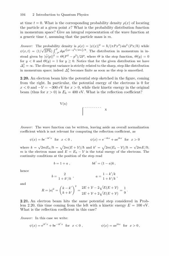
104 2 Introduction to Quantum Physics
at time t = 0. What is the corresponding probability density ρ(x) of locatingthe particle at a given point x? What is the probability distribution functionin momentum space? Give an integral representation of the wave function ata generic time t, assuming that the particle mass is m.
Answer: The probability density is ρ(x) = |ψ(x)|2 = h/(πPx2) sin2 (Px/h) while
ψ(x, t) = (1/√
2Ph)∫ P
−Pdqei(qx−q2t/2m)/h. The distribution in momentum in in-
stead given by |ψ(p)|2 = Θ(P 2 − p2)/2P , where Θ is the step function, Θ(y) = 0
for y < 0 and Θ(y) = 1 for y ≥ 0. Notice that for the given distribution we have
Δ2x =∞. The divergent variance is strictly related to the sharp, step-like distribution
in momentum space; indeed Δ2x becomes finite as soon as the step is smoothed.
2.20. An electron beam hits the potential step sketched in the figure, comingfrom the right. In particular, the potential energy of the electrons is 0 forx < 0 and −V = −300 eV for x > 0, while their kinetic energy in the originalbeam (thus for x > 0) is Ek = 400 eV. What is the reflection coefficient?
. . . . . . . . . .V(x)
x
Answer: The wave function can be written, leaving aside an overall normalizationcoefficient which is not relevant for computing the reflection coefficient, as
ψ(x) = be−ik′x for x < 0 , ψ(x) = e−ikx + aeikx for x > 0
where k =√
2mEk/h =√
2m(E + V)/h and k′ =√
2m(Ek − V)/h =√
2mE/h;m is the electron mass and E = Ek − V is the total energy of the electrons. Thecontinuity conditions at the position of the step read
b = 1 + a , bk′ = (1− a)k ,
hence
b =2
1 + k′/k, a =
1− k′/k
1 + k′/k,
and
R = |a|2 =
(k − k′
k + k′
)2
=2E + V − 2
√E(E + V)
2E + V + 2√
E(E + V)=
1
9.
2.21. An electron beam hits the same potential step considered in Prob-lem 2.20, this time coming from the left with a kinetic energy E = 100 eV.What is the reflection coefficient in this case?
Answer: In this case we write:
ψ(x) = eik′x + be−ik′x for x < 0 , ψ(x) = aeikx for x > 0 ,

Problems 105
where again k =√
2m(E + V)/h and k′ =√
2mE/h with E = Ek being the totalenergy. By solving the continuity conditions we find:
b =k′/k − 1
1 + k′/k; R = |b|2 =
(k′ − k
k + k′
)2
=2E + V − 2
√E(E + V)
2E + V + 2√
E(E + V)=
1
9.
We would like to stress that the reflection coefficient coincides with that obtainedin Problem 2.20: electron beams hitting the potential step from the right or fromthe left are reflected in exactly the same way, if their total energy E is the same,as it is in the present case. In fact this is a general result which is valid for everykind of potential barrier and derives directly from the invariance of the Schrodingerequation under time reversal: the complex conjugate of a solution is also a solution.It may seem a striking result, but it should not be so striking for those familiar withreflection of electromagnetic signals in presence of unmatching impedances.
Notice also that there is actually a difference between the two cases, consisting
in a different sign for the reflected wave. That is irrelevant for computing R but
significant for considering interference effects involving the incident and the reflected
waves. In the present case interference is destructive, hence the probability density
is suppressed close to the step, while in Problem 2.20 the opposite happens. To
better appreciate this fact consider the analogy with an oscillating rope made up
of two different ropes having different densities (which is a system in some sense
similar to ours), and try to imagine the different behaviors observed if you enforce
oscillations shaking the rope from the heavier (right-hand in our case) or from the
lighter (left-hand in our case) side. As extreme and easier cases you could think of a
single rope with a free end (one of the densities goes to zero) or with a fixed end (one
of the densities goes to infinity): the shape of the rope at the considered endpoint is
cosine-like in the first case and sine-like in the second case, exactly as for the cases
of respectively the previous and the present problem in the limit V → ∞.
2.22. An electron beam hits, coming from the right, a potential step similarto that considered in Problem 2.20. However this time −V = −10 eV and thekinetic energy of the incoming electrons is Ek = 9 eV. If the incident currentis equal to J = 10−3 A, compute how many electrons can be found, at a giventime, along the negative x axis, i.e. how many electrons penetrate the stepbarrier reaching positions which would be classically forbidden.
Answer: The solution of the Schrodinger equation can be written as
ψ(x) = c ep′x/h for x < 0 , ψ(x) = a eipx/h + b e−ipx/h for x > 0
where p =√
2mE and p′ =√
2m(V − E). Imposing continuity in x = 0 for bothψ(x) and its derivative, we obtain c = 2a/(1 + ip′/p) and b = a(1− ip′/p)/(1 + ip′/p).It is evident that |b|2 = |a|2, hence the reflection coefficient is one. Indeed the prob-ability current J(x) = −ih/(2m)(ψ∗∂xψ − ψ∂xψ∗) vanishes on the left, where wehave an evanescent wave function, hence no transmission. Nevertheless the prob-ability distribution is non-vanishing for x < 0 and, on the basis of the collectiveinterpretation, the total number of electrons on the left is given by
N =
∫ 0
−∞|ψ(x)|2dx = |c|2h/(2p′) =
2|a|2hp2
p′(p2 + p′2).

106 2 Introduction to Quantum Physics
The coefficient a can be computed by asking that the incident current Jel = eJ =
e|a|2p/m ≡ 10−3 A. The final result is N � 1.2.
2.23. An electron is confined inside a cubic box with reflecting walls and anedge of length L = 2 10−9 m. How many stationary states can be found withenergy less than 1 eV? Take into account the spin degree of freedom, whichin practice doubles the number of available levels.
Answer: Energy levels in a cubic box are Enx,ny,nz = π2h2(n2x + n2
y + n2z)/(2mL2),
where m = 0.911 10−30 Kg and nx, ny , nz are positive integers. The constraint
E < 1 eV implies n2x +n2
y +n2z < 10.7, which is satisfied by 7 different combinations
((1,1,1), (2,1,1), (2,2,1) plus all possible different permutations). Taking spin into
account, the number of available levels is 14.
2.24. When a particle beam hits a potential barrier and is partially transmit-ted, a forward going wave is present on the other side of the barrier which,besides having a reduced amplitude with respect to the incident wave, hasalso acquired a phase factor which can be inferred by the ratio of the trans-mitted wave coefficient to that of the incident one. Assuming a thin barrierdescribable as
V (x) = v δ(x) ,
and that the particles be electrons of energy E = 10 eV, compute the valueof v for which the phase difference is −π/4.
Suppose now that we have two beams of equal amplitude and phase andthat one beam goes through the barrier while the other goes free. The twobeams recombine after paths of equal length. What is the ratio of the recom-bined beam intensity to that one would have without the barrier?
Answer: On one side of the barrier the wave function is ei√
2mEx/h + a e−i√
2mEx/h,
while it is b ei√
2mEx/h on the other side. Continuity and discontinuity constraintsread 1+ a = b and b− 1+ a =
√2m/Evb/h , from which b = (1 + i
√m/2Ev/h)−1
can be easily derived. Requiring that the phase of b be −π/4 is equivalent to√m/2Ev/h = 1, hence v � 2.0 10−28 J m.
With this choice of v the recombined beam is [1+1/(1 + i)]ei√
2mEx/h. The ratio
of the intensity of the recombined beam to that one would have without the barrier
is |[1 + 1/(1 + i)]/2|2 = 5/8.
2.25. If a potential well in one dimension is so thin as to be describable by aDirac delta function:
V (x) = −V Lδ(x)
where V is the depth and L the width of the well, then it is possible tocompute the bound state energies by recalling that for a potential energy ofthat kind the wave function is continuous while its first derivative has thefollowing discontinuity:
limε→0
(∂xψ(x + ε)− ∂xψ(x − ε)) = −2m
h2 V Lψ(0) .
Problems 107
What are the possible energy levels?
Answer: The bound state wave function is
a e−√
2mBx/h for x > 0 and a e√
2mBx/h for x < 0
where the continuity condition for the wave function has been already imposed.
B = |E| is the absolute value of the energy (which is negative for a bound state).
The discontinuity condition on the first derivative leads to an equation for B which
has only one solution, B = mV 2L2/(2h2), thus indicating the existence of a single
bound state.
2.26. A particle of mass m moves in the following one-dimensional potential:
V (x) = v(αδ(x − L) + αδ(x + L)− 1
LΘ(L2 − x2)) ,
where Θ is the step function, Θ(y) = 0 for y < 0 and Θ(y) = 1 for y > 0.Constants are such that
2mvL
h2 =(π
4
)2
.
For what values of α > 0 are there any bound states?
Answer: The potential is such that V (−x) = V (x): in this case the lowest en-ergy level, if any, corresponds to an even wave function. We can thus limit thediscussion to the region x > 0, where we have ψ(x) = cos kx for x < L and
ψ(x) = ae−βx for x > L, with the constraint 0 < k <√
2mv/(h2L) = π/(4L),
since β =√
2mv/(h2L) − k2 must be real in order to have a bound state, hencekL < π/4. Continuity and discontinuity constraints, respectively on ψ(x) and ψ′(x)in x = L, give: tan kL = (β + 2mvα/h2)/k. Setting y ≡ kL, we have
tan y =
√π2
16− y2 + π2
16α
y.
The function on the left hand side grows from 0 to 1 in the interval 0 < y < π/4,
while the function on the right decreases from ∞ to απ/4 in the same interval.
Therefore an intersection (hence a bound state) exists only if α < 4/π.
2.27. An electron moves in a one-dimensional potential corresponding to asquare well of depth V = 0.1 eV and width L = 3 10−10 m. Show that inthese conditions there is only one bound state and compute its energy in thethin well approximation, discussing also the validity of that limit.
Answer: There is one only bound state if the first odd state is absent. Thatis true if y =
√2mV L/(2h) < π/2, which is verified in our case since, using
m = 0.911 10−30 Kg, one obtains y � 0.243 < π/2.Setting B ≡ −E, where E is the negative energy of the bound state, B is
obtained as a solution of

108 2 Introduction to Quantum Physics
tan
(L√
2m(V −B)
2h
)=
√B
V −B.
The thin well limit corresponds to V → ∞ and L → 0 as the product V L is keptconstant. Neglecting B with respect to V we can write
tan
(√2mV L2
2h
)=
√B
V.
In the thin well limit V L2 → constant ·L → 0, hence we can replace the tangent by
its argument, obtaining finally B = mV 2L2/(2h2) � 0.59 10−2 eV, which coincides
with the result obtained in Problem 2.25. In this case the argument of the tangent
is y ∼ 0.24 and we have tan 0.24 � 0.245; therefore the exact result differs from that
obtained in the thin well approximation by roughly 4 %.
2.28. An electron moves in one dimension and is subject to forces correspond-ing to a potential energy:
V (x) = V [−δ(x) + δ(x− L)] .
What are the conditions for the existence of a bound state and what is itsenergy if L = 10−9 m and V = 2 10−29 J m ?
Answer: A solution of the Schrodinger equation corresponding to a binding en-ergy B ≡ −E can be written as
ψ(x) = e√
2mBx/h for x < 0 ,
ψ(x) = ae√
2mBx/h + be−√
2mBx/h for 0 < x < L ,
ψ(x) = ce−√
2mBx/h for L < x .
Continuity and discontinuity constraints, respectively for the wave function and forits derivative in x = 0 and x = L, give: a + b = 1 , a − b − 1 = −
√2m/BV/h ,
ae√
8mBL/h + b = c , ae√
8mBL/h − b + c = −c√
2m/BV/h .
The four equations are compatible if e√
8mBL/h = (1− 2Bh2
mV2 )−1, which has a
non-trivial solution B �= 0 for any L > 0 . Setting y =√
2B/mh/V the compatibil-
ity condition reads e2mVLy/h2
= 1/(1− y2) . Using the values of L and V given in
the text one obtains e2mVL/h2 � 1, hence 2Bh2/(mV2) � 1 within a good approx-imation, i.e. B � mV2/(2h2), which coincides with the result obtained in presenceof a single thin well. This approximation is indeed equivalent to the limit of a large
distance L (hence e2mVL/h2 � 1) between the two Dirac delta functions; it can beeasily verified that in the same limit one has b � 1 and a � 0, so that, in practice,the state is localized around the attractive delta function in x = 0, which is thebinding part of the potential, and does not feel the presence of the other term inthe potential which is very far away.
As L is decreased, the binding energy lowers and the wave function amplitude,
hence the probability density, gets asymmetrically shifted on the left, until the bind-
ing energy vanishes in the limit L → 0. In practice, the positive delta function in

Problems 109
x = L acts as a repulsive term which asymptotically extracts, as L → 0, the particle
from its thin well.
2.29. A particle of mass M = 10−26 Kg moves along the x axis under theinfluence of an elastic force of constant k = 10−6 N/m. The particle is in itsground state: compute its wave function and the mean value of x2, given by
〈x2〉 =
∫∞−∞ dxx2|ψ(x)|2∫∞−∞ dx|ψ(x)|2 .
Answer:
ψ(x) =(
kM
π2h2
)1/8
e−√
kMx2/2h ; 〈x2〉 =1
2
h√kM
� 5 10−19m2 .
2.30. A particle of mass M = 10−25 Kg moves in a 3-dimensional isotropicharmonic potential of elastic constant k = 10 N/m. How many states haveenergy less than 2 10−2 eV?
Answer: Enx.ny,nz = h√
k/M(3/2+nx+ny+nz). Therefore Enx.ny,nz < 2·10−2 eV
is equivalent to nx+ny+nz < 1.54, corresponding to 4 possible states, (nx, ny, nz) =
(0,0,0), (1,0,0), (0,1,0), (0,0,1).
2.31. A particle of mass M = 10−26 Kg moves in one dimension under theinfluence of an elastic force of constant k = 10−6 N/m and of a constant forceF = 10−15 N acting in the positive x direction. Compute the wave functionof the ground state and the corresponding mean value of the coordinate x,given by
〈x〉 =
∫∞−∞ dxx|ψ(x)|2∫∞−∞ dx|ψ(x)|2 .
Answer: As in the analogous classical case, the problem can be brought back toa simple harmonic oscillator with the same mass and elastic constant by a simplechange of variable, y = x − F/K, which is equivalent to shifting the equilibriumposition of the oscillator. Hence the energy levels are the same as for the harmonicoscillator and the wave function of the ground state is
ψ(x) =(
kM
π2h2
)1/8
e−√
kM2h
(x−F/k)2 ,
while 〈x〉 = F/k = 10−9 m.
2.32. A particle of mass m = 10−30 Kg and kinetic energy equal to 50 eV hitsa square potential well of width L = 2 10−10 m and depth V = 1 eV. Whatis the reflection coefficient computed up to the first non-vanishing order in V
2E ?

110 2 Introduction to Quantum Physics
Answer: Let us choose the square well endpoints in x = 0 and x = L and fixthe potential to zero outside the well. Let ψs, ψc and ψd be respectively the wavefunctions for x < 0, 0 < x < L and x > L. If the particle comes from the left, then
ψs = ei√
2mEx/h + a e−i√
2mEx/h, ψc = b ei√
2m(E+V )x/h + c e−i√
2m(E+V )x/h and
ψd = d ei√
2mEx/h where a and c are necessarily of order V/2E while b and d areequal to 1 minus corrections of the same order. Indeed, as V → 0 the solution musttend to a single plane wave. By applying the continuity constraints we obtain:
1 + a = b + c ,
1− a � b− c +V
2E,
bei√
2m(E+V )L
h + c e−i√
2m(E+V )L/h � (b +V
2E)ei√
2m(E+V )Lh − c e−i√
2m(E+V )L/h ,
which are solved by a � V4E
(e2i√
2m(E+V )L/h − 1) and
R =V 2
4E2sin2
(√2m(E + V )L
h
)� 0.96 10−4 .
2.33. A particle of mass m = 10−30 Kg is confined inside a line segment oflength L = 10−9 m with reflecting endpoints, which is centered around theorigin. In the middle of the line segment a thin repulsive potential barrier,describable as V (x) = Wδ(x), acts on the particle, with W = 2 10−28 J m.Compare the ground state of the particle with what found in absence of thebarrier.
Answer: Let us consider how the solutions of the Schrodinger equation in a line seg-ment are influenced by the presence of the barrier. Odd solutions, contrary to evenones, do not change since they vanish right in the middle of the segment, so that theparticle never feels the presence of the barrier. In order to discuss even solutions, letus notice that they can be written, shifting the origin in the left end of the segment,as ψs ∼ sin (
√2mEx/h) for x < L/2 and ψd ∼ sin (
√2mE(L− x)/h) for x > L/2.
Setting z ≡ √2mEL/(2h) the discontinuity in the wave function derivative in themiddle of the segment gives tan z = −z2h2/(mLW ) � −10−1 z. Hence we obtain,
for the ground state, E � 2h2
mL2 π2(1 − 2 10−1) � 2.75 10−19 J, slightly below thefirst excited level.
Notice that, increasing the intensity of the repulsive barrier W from 0 to ∞, the
fundamental level grows from π2h2/(2mL2) to 2π2h2/(mL2), i.e. it is degenerate
with the first excited level in the W →∞ limit. There is no contradiction with the
expected non-degeneracy since, in that limit, the barrier acts as a perfectly reflecting
partition wall which separates the original line segment in two non-communicating
segments: the two degenerate lowest states (as well as all the other excited ones)
can thus be seen as two different superpositions (symmetric and antisymmetric) of
the ground states of each segment.
2.34. An electron beam corresponding to an electric current I = 10−12 Ahits, coming from the right, the potential step sketched in the figure. The
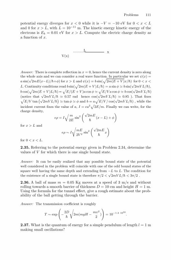
Problems 111
potential energy diverges for x < 0 while it is −V = −10 eV for 0 < x < Land 0 for x > L, with L = 10−11 m. The kinetic energy kinetic energy of theelectrons is Ek = 0.01 eV for x > L. Compute the electric charge density asa function of x.
..........V(x)
xL
Answer: There is complete reflection in x = 0, hence the current density is zero alongthe whole axis and we can consider a real wave function. In particular we set ψ(x) =
a sin(√
2mE(x−L)/h+φ) for x > L and ψ(x) = b sin(√
2m(E + V )x/h) for 0 < x <
L. Continuity conditions read b sin(√
2m(E + V )L/h) = a sin φ � b sin(√
2mV L/h),
b cos(√
2m(E + V )L/h) =√
E/(E + V )a cos φ �√
E/V a cos φ � b cos(√
2mV L/h)
(notice that√
2mV L/h � 0.57 rad hence cos(√
2mV L/h) � 0.85 ). That fixes√E/V tan
(√2mV L/h
)� tan φ � φ and b = a
√E/V / cos(
√2mV L/h) , while the
incident current fixes the value of a, I = ea2√
2E/m. Finally we can write, for thecharge density,
eρ = I√
m
2Esin2
(√2mE
h(x− L) + φ
)for x > L and
eρ ∼ I
√mE
2V 2sin2
(√2mE
hx
)for 0 < x < L.
2.35. Referring to the potential energy given in Problem 2.34, determine thevalues of V for which there is one single bound state.
Answer: It can be easily realized that any possible bound state of the potential
well considered in the problem will coincide with one of the odd bound states of the
square well having the same depth and extending from −L to L. The condition for
the existence of a single bound state is therefore π/2 <√
2mV L/h < 3π/2 .
2.36. A ball of mass m = 0.05 Kg moves at a speed of 3 m/s and withoutrolling towards a smooth barrier of thickness D = 10 cm and height H = 1 m.Using the formula for the tunnel effect, give a rough estimate about the prob-ability of the ball getting through the barrier.
Answer: The transmission coefficient is roughly
T ∼ exp
(−2D
h
√2m(mgH − mv2
2)
)= 10−1.3 1032
.
2.37. What is the quantum of energy for a simple pendulum of length l = 1 mmaking small oscillations?
112 2 Introduction to Quantum Physics
Answer: In the limit of small oscillations the pendulum can be described as a
harmonic oscillator of frequency ν = 2πω = 2π√
g/l, where g � 9.8 m/s is the
gravitational acceleration on the Earth surface. The energy quantum is therefore
hν = 3.1 10−34 J.
2.38. Compute the mean value of x2 in the first excited state of a harmonicoscillator of elastic constant k and mass m.
Answer: The wave function of the first excited state is ψ1 ∝ x e−x2√
km/(4h2),hence
〈x2〉 =
∫∞−∞ x4e−x2
√km/h2
dx∫∞−∞ x2e−x2
√km/h2
dx=
3
2
√h2
km.
2.39. A particle of mass M moves in a line segment with reflecting endpointsplaced at distance L. If the particle is in the first excited state (n = 2), whatis the mean quadratic deviation of the particle position from its average value,i.e.
√〈x2〉 − 〈x〉2 ?
Answer: Setting the origin in the middle of the segment, the wave function isψ(x) =
√2/L sin(2πx/L) inside the segment and vanishes outside. Obviously
〈x〉 = 0 by symmetry, while
〈x2〉 =2
L
∫ L2
− L2
x2 sin2(
2πx
L
)dx = L2
(1
12− 1
8π2
)whose square root gives the requested mean quadratic deviation.
2.40. An electron beam of energy E hits, coming from the left, the followingpotential barrier: V (x) = Vδ(x) where V is tuned to h
√2E/m. Compute the
probability density on both sides of the barrier.
Answer: The wave function can be set to eikx + a e−ikx for x < 0 and to b eikx forx > 0, where k =
√2mE/h. Continuity and discontinuity constraints for ψ and ψ′
in x = 0 lead to
a =1
ikh2
mV − 1=
1
i− 1, b =
ikh2
mVikh2
mV − 1=
1
i + 1.
The probability density is therefore ρ = 1/2 for x > 0, while for x > 0 it is ρ =
3/2−√2 sin(2kx + π/4).
2.41. A particle moves in one dimension under the influence of the potentialgiven in Problem 2.34. Assuming that
√2mV
L
h=
π
2+ δ , with δ � 1 ,
show that, at the first non-vanishing order in δ , one has B � V δ2, whereB = −E and E is the energy of the bound state. Compute the ratio of the

Problems 113
probability of the particle being inside the well to that of being outside.
Answer: The depth of the potential is slightly above the minimum for having
at least one bound state (see the solution of Problem 2.36), therefore we expect
a small binding energy. In particular the equation for the bound state energy, which
can be derived by imposing the continuity constraints, is cot(√
2m(V −B)L/h)
=
−√
B/(V −B). The particular choice of parameters implies B � V , so that
cot(√
2m(V −B)L/h)� cot(π/2(1−B/(2V ))+ δ) � −δ +πB/(4V ) � −
√B/V ,
hence B � V δ2. Therefore the wave function is well approximated by k sin (πx/2L)
inside the well and by ke−√
2mB(x−L)/h � ke−πδ(x−L)/2L outside, where k is a nor-
malization constant. The ratio of probabilities is πδ/2: the very small binding energy
is reflected in the large probability of finding the particle outside the well.
2.42. A particle of mass m = 10−30 Kg and kinetic energy E = 13.9 eV hitsa square potential barrier of width L = 10−10 m and height V = E. Computethe reflection coefficient R.
Answer: Let us fix in x = 0 and in x = L the edges of the square poten-tial barrier, and suppose the particle comes from the left. The wave functionis ψ(x) = eikx + a e−ikx for x < 0 and ψ(x) = d eikx for x > L, wherek =
√2mE/h � 2 1010 m−1. Instead for 0 ≤ x ≤ L the wave function satisfies
the differential equation ψ′′ = 0, which has the general integral ψ(x) = bx + c. Thecontinuity conditions for ψ and ψ′ in x = 0 and x = L read
1 + a = c ; ik (1− a) = b ; bL + c = d eikL ; b = ik d eikL .
Dividing last two equations and substituting the first two we get
a =ikL
ikL− 2; R = |a|2 =
k2L2
4 + k2L2� 1
2.
It is interesting to verify that the same result can be obtained by taking carefully
the limit E → V in equation (2.72).
2.43. A particle whose wave function is, for asymptotically large negativetimes (that is −t� m/(hk0Δ)), a Gaussian wave packet
ψ(x, t) =1√
(2π)3/2Δ
∫dkei(kx−hk2t/(2m))e−(k−k0)2/(2Δ)2
with k0/Δ � 1, interacts in the origin through the potential V (x) = Vδ(x)and its wave function splits into reflected and transmitted components. Con-sidering values of the time for which the spreading of the packets can beneglected, that is |t| � m/(hΔ2) (see Section 2.4), compute the transmittedand reflected components of the wave packet.
Answer: The Gaussian wave packet has been studied in detail in Section 2.4, itis therefore straightforward to check that, for large negative times, the solution that

114 2 Introduction to Quantum Physics
we are seeking is a wave packet centered in x = vt, with v = hk0/m, i.e. a packetapproaching the barrier from the left and hitting it at t � 0.
It has been shown in Section 2.5.2 (see also Problem 2.24) that the genericsolution of the time independent Schrodinger equation, obtained in the case of asingle plane wave eikx hitting the barrier from the left, is
ψk(x) = Θ(−x)[exp(ikx)− iκ/(k + iκ) exp(−ikx)] + Θ(x)k/(k + iκ) exp(ikx)
where Θ is the step function (Θ(x) = 0 for x < 0 and Θ(x) = 1 for x ≥ 0) andκ = mV/h2.
The present problem consists in finding a solution of the time dependentSchrodinger equation which, for asymptotically large negative times and x < 0,must be a given superposition of progressive plane waves corresponding to the in-coming wave packet. Given the linearity of the Schrodinger equation, the solutionmust be a linear superposition of the generic solutions given above, with the samecoefficients of the incoming packet, i.e.
ψ(x, t) =1√
(2π)3/2Δ
∫dk ψk(x)e−ihk2t/(2m)e−(k−k0)2/(2Δ)2 .
This decomposes into two components for x < 0 and a single transmitted componentfor x > 0.
The first, ingoing component on the negative semi-axis, which corresponds toψk(x) = exp(ikx), is a standard Gaussian packet which, as discussed above, crossesthe origin for t ∼ 0 and hence disappears for larger times. On the contrary, aswe shall show in while, the second, reflected component describes a packet movingbackward, which crosses the origin for t ∼ 0, hence appears as a part of the solutionfor x < 0 for positive times (i.e. after reflection of the original packet), when it mustbe taken into account. In much the same way we shall compute the transmittedcomponent, which is a packet moving forward and which appears on the positivesemi-axis for positive times. Now we work out the details, this can be done usingequation (2.52).
We represent the transmitted and reflected wave packets by
1√(2π)3/2Δ
∫ ∞
−∞dt exp(−FT/R(k, x, t))
FT (k, x, t) = (k − k0)2/(2Δ)2 − i(kx− hk2t/(2m))− ln(k/(k + iκ))
FR(k, x, t) = (k − k0)2/(2Δ)2 + i(kx + hk2t/(2m))− ln(−iκ/(k + iκ)) .
Then we have the equations:
∂kFT (k, x, t) = (k − k0)/Δ2 − i(x− htk/m + κ/(k(k + iκ))) = 0
∂kFR(k, x, t) = (k − k0)/Δ2 + i(x + htk/m− i/(k + iκ)) = 0 .
The equation for FT has three solutions: k1 ∼ k0, k2 ∼ 0 and k3 ∼ −iκ up tocorrections of order Δ2. The first solution has a second derivative of order 1/Δ2,to be compared with the second derivatives of the other two solutions, which areof order 1/Δ4, hence it is the dominant solution, in the same sense discussed inSection 2.4 (see equation (2.52)), thus we concentrate on it. Setting again v = hk0/mwe have k1 = k0 + iΔ2(x− vt + κ/(k0(k0 + iκ))) + O(Δ4) and

Problems 115
FT (k1, x, t) = FT (k0, x, t)− ∂2kFT (k0, x, t)(k1 − k0)
2/2 =
−i(k0x− hk20t/(2m))− ln(k0/(k0 + iκ))+ [x− vt+κ/(k0(k0 + iκ))]2Δ2/2)+O(Δ4) .
Therefore we have a wave packet centered in x = vt − κ/(k20 + κ2). An analogous
analysis on the reflected packet gives:
FR(k1, x, t) = FR(k0, x, t)− ∂2kFR(k0, x, t)(k1 − k0)
2/2 =
i(k0x + hk20t/(2m))− ln(−iκ/(k0 + iκ)) + (x + vt− i/(k0 + iκ))2Δ2/2) + O(Δ4) .
Now the packet is centered in x = −vt + κ/(k20 + κ2) .
The result is almost as anticipated, apart from the fact that the appearance of
the transmitted and reflected wave packets is delayed (advanced) with respect to the
time the incoming packet hits the potential barrier (well). For large, positive times
the particle is in a superposition of reflected and transmitted state, the probability of
finding it in one of the two states after a measurement of its position (i.e. the integral
of the probability density over the corresponding packets) is given approximately by
the reflection or transmission coefficients computed for k ∼ k0.
2.44. A particle of mass m moves in one dimension under the influence of thepotential
V (x) = V0Θ(x) − Vδ(x) .
If V = 3 10−29 J m and m = 10−30 Kg, identify the values of V0 for whichthe particle has bound states. Assuming the existence of a bound state whosebinding energy is B � V0, compute the ratio of the probabilities for the par-ticle to be found on the right and on the left-hand side of the origin.
Answer: The wave function of a bound state with energy −B would be
ψB(x) = N [Θ(−x) exp(√
2mBx/h) + Θ(x) exp(−√
2m(B + V0)x/h)]
where Θ is the step function, N is the normalization factor and the condition√
B +√B + V0 =
√2mV/h must be satisfied. Since
√V0 ≤
√B+
√B + V0 < ∞ the above
condition has a solution provided√
2mV/h ≥ √V0, hence for V0 ≤ 2mV2/h2 �
1.62 10−19 J � 1 eV. The probabilities for the particle to be found on the right and
on the left of the origin are respectively N2h/(2√
2m(B + V0)) and N2h/(2√
2mB),
their ratio for small B is√
B/V0 �√
2m/V0V/h− 1.
2.45. A particle of mass m is bound between two spherical perfectly reflect-ing walls of radii R and R + Δ. The potential energy between the wallsis V0 = −h2π2/(2mΔ2). If the total energy of the particle cannot exceedEM = 6h2/(2mR2) compute, in the Δ → 0 limit in which the particle isbound on the sphere of radius R, the maximum possible value of its superfi-cial probability density on the intersection point of the sphere with the positivez axis.
Answer: In the Δ → 0 limit, the radial Schrodinger equation tends to the one-dimensional Schrodinger equation of a particle between two reflecting walls with po-tential energy between the walls equal to V = −h2π2/(2mΔ2) + l(l + 1)h2/(2mR2)

116 2 Introduction to Quantum Physics
(see equation(2.177)). Therefore the possible energy values are En,l = (n2 −1)h2π2/(2mΔ2) + l(l + 1)h2/(2mR2). Only the energies E1,l = l(l + 1)h2/(2mR2)remain finite as Δ → 0. In spherical coordinates, the corresponding wave functionsare, in the Δ → 0 limit, Ψl,m =
√2/(ΔR2) sin(π(r −R)/Δ)Yl,m(θ, φ).
The harmonic functions Yl,m with m �= 0 are proportional to powers of x±(see equations (2.165) and (2.178)), hence they vanish on the z axis, therefore and
on account of the energy bound, among the possible solutions, we only consider
Ψl,0 for 0 ≤ l ≤ 2. Forgetting the radial dependence which, in the Δ → 0 limit
corresponds to a probability density equal to δ(r −R), these are Ψ0,0 = 1/(R√
4π),
Ψ1,0 =√
3/4π cos θ/R and Ψ2,0 =√
5/16π (3 cos2 θ − 1)/R. The wave function of
the particle with the above constraints is written as the linear combination a0 Ψ0,0 +
a1 Ψ1,0 + a2 Ψ2,0, with the normalization condition |a0|2 + |a1|2 + |a2|2 = 1 . On
the positive z axis the wave function is 1/√
4π[a0 +√
3a1 +√
5a2]/R2 . It is fairly
obvious that the maximum absolute value is reached when a0 = a1 = 0, hence the
maximum superficial probability density of the particle is 5/(4πR2). The result can
be generalized to the case in which different values of the angular momentum can be
reached, indeed it can be proved, considering equations (2.171), (2.172) and (2.173),
that |Ψl,0(θ = 0)|2 = (2l + 1)/(4πR2).
2.46. A particle of mass m moves in three dimensions under the influence ofthe central potential V (r) = −h2α/(2mR) δ(r−R), with α positive. Computethe values of α for which the particle has a bound state with non-zero angularmomentum.
Answer: For zero angular momentum (S-wave), the solution to the differentialequation for the radial wave function χ(r) defined in equation (2.178), satisfying theregularity conditions in the origin and at infinity, is equivalent to the odd solutionfor the one-dimensional double well potential given in Problem 2.47 (setting L = R),hence χ< ∝ sinh(kr) for r < R and χ> ∝ exp(k(R− r)) for r > R, the bound stateenergy being E = −h2k2/(2m) with k > 0 . We know, from Problem 2.47, that suchsolution exists only if α > 1.
We consider now the P-wave case (l = 1). The solution satisfying the correct
regularity conditions can be obtained from that written in the S-wave case by ap-
plying the recursive equation (2.184). It is, up to an overall normalization factor,
χ< = sinh(kr)/(kr)− cosh(kr) for r < R and χ> = a exp(k(R− r))[1/(kr) + 1] for
r > R. The continuity conditions at r = R, written in terms of kR = x, are given by
sinh x/x−coshx = a(1+x)/x and cosh x/x−sinhx(1+x2)/x2+a(1+1/x+1/x2) =
α(sinh x/x2−cosh x/x) , from which we have tanh x = x(1+x−x2/α)/(1+x+x3/α) .
We know that the graphs of both sides of this equation cross at most once for x > 0
since we have seen in the one-dimensional case, e.g. in Section (2.6), that a thin po-
tential well has at most a single bound state. It remains to be verified if they cross.
The graphs are tangent to each other in the origin and, for x →∞, the left-hand side
tends to +1 and the right-hand side to −1, therefore if the left-hand side is steeper
in the origin the graphs do not cross, otherwise they cross once and there is a bound
state. Considering the Taylor expansions of both sides we have tanh x � x − x3/3
and x(1 + x − x2/α)/(1 + x + x3/α) � x − x3/α . The conclusion is that there is
a bound state if α > 3. It should be clear that if no bound state can be found for

Problems 117
l = 1 (i.e. α < 3), none will be found for l > 1 as well, because of the increased
centrifugal potential.
2.47. A particle of mass m moves along the x axis under the influence of thedouble well potential:
V (x) = −V [δ(x + L) + δ(x− L)] ,
with V > 0 . Study the solutions of the stationary Schrodinger equation. Sincethe potential is even under x reflection, the solutions are either even or odd.Show that in the even case there is a single solution for any value of L, dis-cuss the range of values of the binding energy B and, in particular, how Bdepends on L for small L, i.e. when α(L) ≡ 2mVL/h2 � 1. Compute the“force” between the two wells in this limit. In the odd solution case, computethe range of α(L) for which there are bound solutions and compare the evenwith the odd binding energies.
Answer: Starting from the even case, we write the solution between the wellsas ψI(x) = cosh kx, with B = h2k2/(2m), and the external solution as ψE(x) =a exp(−k(|x| − L)). The continuity conditions on the wells give: a = cosh(kL) andk(sinh(kL)+a) = α(L) cosh(kL)/L. Setting kL = y we get the transcendental equa-tion tanh y = α(L)/y−1. This equation has a single solution y(α(L)), correspondingto a single bound state, for any positive value of α(L). In particular for small α(L)also y(α(L)) is small and the equation is approximated by y − y3/3 = α(L)/y − 1which, up to the second order in α(L), has the positive y solution y(α(L)) =α(L) − α2(L). The corresponding binding energy is computed noticing that B =h2y2/(2mL2), from which we have B = 2mV2/h2 − 8m2V3L/h4 + O(α4(L)). Thisimplies that there is an attractive force between the two wells which, in the smallα(L) limit, is equal to F = 8m2V3/h4, furthermore B ≤ Bmax = 2mV2/h2 ; noticethat Bmax is the binding energy for a single well −2Vδ(x), which is indeed the limitof V (x) as L→ 0. For large α(L) also y(α(L)) is large and the transcendental equa-tion is well approximated by 1 = α(L)/y−1, which gives y(α(L)) = α(L)/2, so thatthe binding energy reaches its minimum value Bmin = mV2/(2h2), which coincideswith the binding energy of a single well.
In the odd case the solution between the wells becomes ψI(x) = sinh kx whilethe external one does not change, therefore the transcendental equation becomestanh y = y/(α(L)− y). Here the right-hand side is concave downward and positive,while the left-hand side is concave upward and positive for 0 < y < α(L), it has asingularity in α(L) and it is negative beyond the singularity. Therefore the equationhas a solution for 0 < y < α if, and only if, the left-hand side is steeper in the originthan the right-hand side, that is if α(L) > 1. For large values of α(L), y(α(L)) tendsto α(L)/2 from below; notice that in the even case the same limit is reached fromabove.
In conclusion, for any value of the distance between the two wells, there is an
even solution, whose binding energy is larger than that of a single well; on the
contrary an odd solution exists only if L > h2/(2mV), with a binding energy lower
than that of a single well. In the limit of large separation between the two wells,
both the odd and the even level approach the energy of a single well, one from
above and the other from below, i.e. we get asymptotically two degenerate levels.

118 2 Introduction to Quantum Physics
The presence of two slightly splitted levels (the even ground state and the odd first
excited state) is a phenemenon common to other symmetric double well potentials;
an example is given by the Ammonia molecule (NH3), in which the Nitrogen atom
has two symmetric equilibrium positions on both sides of the plane formed by the
three Hydrogen atoms.
2.48. A particle of mass m is constrained to move on a plane surface where itis subject to an isotropic harmonic potential of angular frequency ω. Whichare the stationary states which are found, for the first excited level, by separa-tion of variables in Cartesian coordinates? Show that the probability currentdensity for such states vanishes. Are there any stationary states belongingto the same level having a non-zero current density? Find those having themaximum possible current density and give a physical interpretation for them.
Answer: For the first excited level, E1 = 2hω, the two following stationary statesare found in Cartesian coordinates (see equations (2.128) and (2.125)):
ψ1,0 =
√2α2x√
πe−α2(x2+y2)/2 ; ψ0,1 =
√2 α2y√
πe−α2(x2+y2)/2
where α =√
mω/h. In both cases the current density
J = − ih
2m(ψ∗
∇ψ − ψ∇ψ∗) =h
mIm (ψ∗
∇ψ)
vanishes, since the wave functions are real. However it is possible to find differentstationary states, corresponding to linear combinations of the two states above,having a non-zero current. Indeed for the most general state, which up to an overallirrelevant phase factor can be written as
ψ = aψ1,0 +√
1− a2eiφψ0,1
where a ∈ [0, 1] is a real parameter, the probability current density is
J =2hα4
mπe−α2(x2+y2) a
√1− a2 sin φ j
where (jx, jy) = (−y, x). The current field is independent, up to an overall factor,of the particular state chosen and describes a circular flow around the origin, hencein general a state with a non-zero average angular momentum; moreover ∇ · J = 0,as expected for a stationary state. The current vanishes for a = 0, 1 or φ = 0, π andis maximum for a = 1/
√2 and φ = ±π/2, corresponding to the states:
ψ± =1√2
(ψ1,0 ± iψ0,1) =α2
√π
e−α2(x2+y2)/2(x± iy) =α2
√π
e−α2r2/2x±
where r2 = x2 + y2, which are easily recognized as the states having a well defined
angular momentum L = ±h (compare for instance with equation (2.150)).
3
Introduction to the Statistical Theory
of Matter
In Chapter 2 we have discussed the existence and the order of magnitudeof quantum effects, showing in particular their importance for microscopicphysics. We have seen that quantum effects are relevant for electrons at ener-gies of the order of the electron-volt, while for the dynamics of atoms in crys-tals, which have masses three or four order of magnitudes larger, significanteffects appear at considerably lower energies, corresponding to low tempera-tures. Hence, in order to study these effects, a proper theoretical framework isneeded for describing systems made up of particles at thermal equilibrium andfor deducing their thermodynamical properties from the (quantum) nature oftheir states.
Boltzmann identified the thermal contact among systems as a series ofshortly lasting and random interactions with limited energy exchange. Theseinteractions can be considered as collisions among components of two differ-ent systems taking place at the surface of the systems themselves. Collisionsgenerate sudden transitions among the possible states of motion for the partsinvolved. The sequence of collision processes is therefore analogous to a seriesof dice casts by which subsequent states of motion are chosen by drawing lots.
It is clear that in these conditions it is not sensible to study the time evo-lution of the system, since that is nothing but a random succession of states ofmotion. Instead it makes sense to study the distribution of states among thoseaccessible to the system, i.e. the number of times a particular state occurs inN different observations. In case of completely random transitions among allthe possible states, the above number is independent of the particular stateconsidered and equal to the number of observations N divided by the totalnumber of possible states. In place of the distribution of results of subsequentobservations we can think of the distribution of the probability that the systembe in a given state: under the same hypothesis of complete randomness, theprobability distribution is independent of the state and equal to the inverseof the total number of accessible states.
However the problem is more complicated if we try to take energy conser-vation into account. Although the energy exchanged in a typical microscopic
120 3 Introduction to the Statistical Theory of Matter
collision is very small, the global amount of energy (heat) transferred in a greatnumber of interactions can be macroscopically relevant; on the other hand,the total energy of all interacting macroscopic systems must be constant.
The american physicist J. Willard Gibbs proposed a method to evaluatethe probability distribution for the various possible states in the case of ther-mal equilibrium1. His method is based on the following points.
1) Thermal equilibrium is independent of the nature of the heat reservoir,which must be identified with a system having infinite thermal capacity (thatis a possible enunciation of the so-called zero-th principle of thermodynamics).According to Gibbs, the heat reservoir is a set of N systems, identical tothe one under consideration, which are placed in thermal contact. N is sogreat that each heat (energy) exchange between the system and the reservoir,being distributed among all different constituent systems, does not alter theiraverage energy content, hence their thermodynamical state.
2) Gibbs assumed transitions to be induced by completely random colli-sions. Instead of following the result of a long series of random transitionsamong states, thus extracting the probability distribution by averaging overtime evolution histories, Gibbs proposed to consider a large number of si-multaneous draws and to take the average over them. That is analogous todrawing a large number of dice simultaneously instead of a single die for alarge number of times: time averages are substituted by ensemble averages.Since in Gibbs scheme the system–reservoir pair (Macrosystem) can be iden-tified with the N +1 identical systems in thermal contact and in equilibrium,if at any time the distribution of the states occupied by the various systems ismeasured, one has automatically an average over the ensemble and the occu-pation probability for the possible states of a single system can be deduced.On the other hand, computing the ensemble distribution does not require theknowledge of the state of each single system, but instead that of the numberof systems in each possible state.
3) The macrosystem is isolated and internal collisions induce randomchanges of its state. However, all possible macrosystem states with the sametotal energy are assumed to be equally probable. That clearly implies that theprobability associated to a given distribution of the N + 1 systems is directlyproportional to the number of states of the macrosystem realizing the givendistribution: this number is usually called multiplicity. If i is the index distin-guishing all possible system states, any distribution is fixed by a successionof integers {Ni}, where Ni is the number of systems occupying state i. It iseasy to verify that the multiplicity M is given by
1 Notice that the states considered by Gibbs in the XIX century were small cellsin the space of states of motion (the phase space) of the system, while we shallconsider quantum states corresponding to independent solutions of the stationarySchrodinger equation for the system. This roughly corresponds to choosing thevolume of Gibbs cells of the order of magnitude of hN , where N is the numberof degrees of freedom of the system.
3 Introduction to the Statistical Theory of Matter 121
M({Ni}) =N !∏i Ni!
, (3.1)
with the obvious constraint ∑i
Ni = N . (3.2)
4) The accessibility criterion for states is solely related to their energywhich, due to the limited energy exchange in collision processes, is reducedto the sum of the energies of the constituent systems. Stated otherwise, if Ei
is the energy of a single constituent system when it is in state i, disregardingthe interaction energy between systems, the total energy of the macrosystemis identified with:
Etot =∑
i
EiNi ≡ NU . (3.3)
Thus U can be identified with the average energy of the constituent systems:it characterizes the thermodynamical state of the reservoir and must thereforebe related to its temperature in some way to be determined by computations.
5) Gibbs identified the probability of the considered system being in statei with:
pi =Ni
N , (3.4)
where the distribution {Ni} is the one having maximum multiplicity amongall possible distributions:
M({Ni}) ≥M({Ni}) ∀ {Ni} ,
i.e. that is realized by the largest number of states of the macrosystem. Wecall pi the occupation probability of state i.
The identification made by Gibbs is justified by the fact that the multiplic-ity function has only one sharp peak in correspondence of its maximum, whosewidth (ΔM/M) vanishes in the limit of an ideal reservoir, i.e. as N → ∞.Later on we shall discuss a very simple example, even if not very significantfrom the physical point of view, corresponding to a system with only threepossible states, so that the multiplicity M, given the two constraints in (3.2)and (3.3), will be a function of a single variable, thus allowing an easy com-putation of the width of the peak.
6) The analysis of thermodynamical equilibrium described above can beextended to the case in which also the number of particles in each systemis variable: not only energy transfer by collisions can take place at the sur-faces of the systems, but also exchange of particles of various species (atoms,molecules, electrons, ions and so on). In this case the various possible states ofthe system are characterized not only by their energy but also by the number
of particles of each considered species. We will indicate by n(s)i the number of
particles belonging to species s and present in state i; therefore, besides theenergy Ei, there will be as many fixed quantities as the number of possible

122 3 Introduction to the Statistical Theory of Matter
species characterizing each possible state of the system. The distribution ofstates in the macrosystem, {Ni}, will then be subject to further constraints,besides (3.2) and (3.3), related to the conservation of the total number ofparticles for each species, namely∑
i
n(s)i Ni = n(s)N (3.5)
for each s. The kind of thermodynamical equilibrium described in this case isvery different from the previous one. While in the first case equilibrium cor-responds to the system and reservoir having the same temperature (T1 = T2),in the second case also Gibbs potential g(s) will be equal, for each con-strained single particle species separately. In place of g(s) it is usual to considerthe quantity known as chemical potential, defined as μ(s) ≡ g(s)/NA, whereNA = 6.02 1023 is Avogadro’s number.
The distributions corresponding to the two different kinds of equilibriumare named differently. For a purely thermal equilibrium we speak of Canoni-
cal Distribution, while when considering also particle number equilibrium wespeak of Grand Canonical Distribution. We will start by studying simple sys-tems by means of the Canonical Distribution and will then make use of theGrand Canonical Distribution for the case of perfect quantum gasses.
As the simplest possible systems we shall consider in particular an isotropicthree-dimensional harmonic oscillator (Einstein’s crystal) and a particle con-fined in a box with reflecting walls. Let us briefly recall the nature of thestates for the two systems.
Einstein’s crystal
In this model atoms do not exchange forces among themselves but in rarecollisions, whose nature is not well specified and whose only role is that ofassuring thermal equilibrium. Atoms are instead attracted by elastic forcestowards fixed points corresponding to the vertices of a crystal lattice.
The attraction point for the generic atom is identified by the coordinates(mxa, mya, mza), where mx, my, mz are relative integer numbers with |mi|a <L/2: L is the linear size and a is the spacing of the crystal lattice, which isassumed to be cubic. To summarize, each atom corresponds to a vector m ofcomponents mx, my, mz.
Hence Einstein’s crystal is equivalent to a large number of isotropic har-monic oscillators and can be identified with the macrosystem itself. Accordingto the analysis of the harmonic oscillator made in previous Chapter, the mi-
croscopic quantum state of the crystal is characterized by three non-negativeinteger numbers (nx,m, ny,m, nz,m) for every vertex (m). The correspondingenergy level is given by
Enx,m,ny,m,nz,m=∑m
h ω
(nx,m + ny,m + nz,m +
3
2
). (3.6)
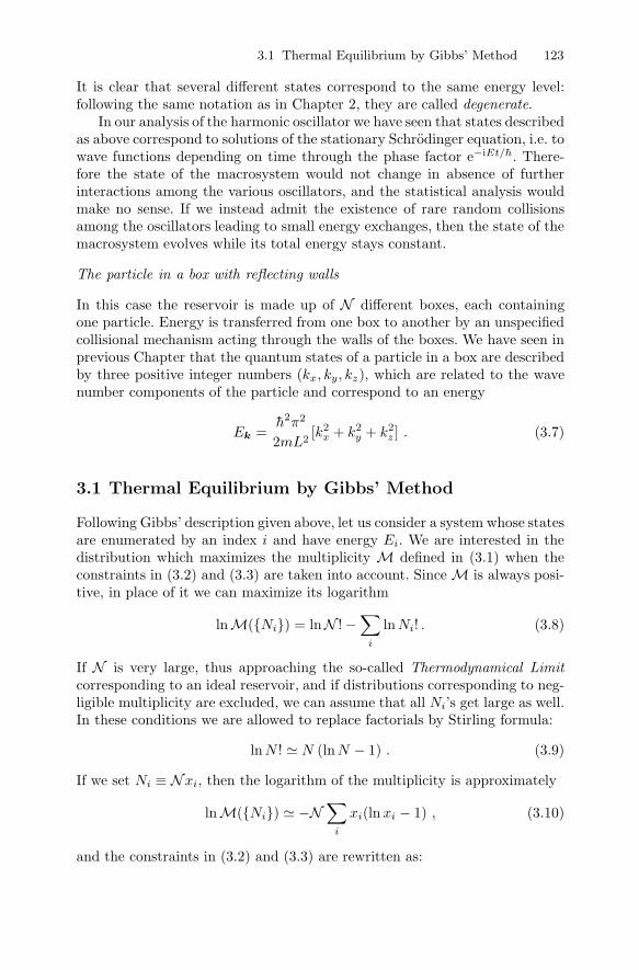
3.1 Thermal Equilibrium by Gibbs’ Method 123
It is clear that several different states correspond to the same energy level:following the same notation as in Chapter 2, they are called degenerate.
In our analysis of the harmonic oscillator we have seen that states describedas above correspond to solutions of the stationary Schrodinger equation, i.e. towave functions depending on time through the phase factor e−iEt/h. There-fore the state of the macrosystem would not change in absence of furtherinteractions among the various oscillators, and the statistical analysis wouldmake no sense. If we instead admit the existence of rare random collisionsamong the oscillators leading to small energy exchanges, then the state of themacrosystem evolves while its total energy stays constant.
The particle in a box with reflecting walls
In this case the reservoir is made up of N different boxes, each containingone particle. Energy is transferred from one box to another by an unspecifiedcollisional mechanism acting through the walls of the boxes. We have seen inprevious Chapter that the quantum states of a particle in a box are describedby three positive integer numbers (kx, ky, kz), which are related to the wavenumber components of the particle and correspond to an energy
Ek =h2π2
2mL2[k2
x + k2y + k2
z ] . (3.7)
3.1 Thermal Equilibrium by Gibbs’ Method
Following Gibbs’ description given above, let us consider a system whose statesare enumerated by an index i and have energy Ei. We are interested in thedistribution which maximizes the multiplicity M defined in (3.1) when theconstraints in (3.2) and (3.3) are taken into account. Since M is always posi-tive, in place of it we can maximize its logarithm
lnM({Ni}) = lnN !−∑
i
ln Ni! . (3.8)
If N is very large, thus approaching the so-called Thermodynamical Limit
corresponding to an ideal reservoir, and if distributions corresponding to neg-ligible multiplicity are excluded, we can assume that all Ni’s get large as well.In these conditions we are allowed to replace factorials by Stirling formula:
ln N ! � N (lnN − 1) . (3.9)
If we set Ni ≡ Nxi, then the logarithm of the multiplicity is approximately
lnM({Ni}) � −N∑
i
xi(lnxi − 1) , (3.10)
and the constraints in (3.2) and (3.3) are rewritten as:

124 3 Introduction to the Statistical Theory of Matter∑i
xi = 1 ,
∑i
Eixi = U . (3.11)
In order to look for the maximum of expression (3.10) in presence of the con-straints (3.11), it is convenient to apply the method of Lagrange’s multipliers.
Let us remind that the stationary points of the function F (x1, ..., xn) inpresence of the constraints: Gj(x1, ..., xn) = 0, with j = 1, ..., k and k < n,are solutions of the following system of equations:
∂
∂xi
⎡⎣F (x1, ..., xn) +
k∑j=1
λjGj(x1, ..., xn)
⎤⎦ = 0 , i = 1, ..., n ,
and of course of the constraints themselves. Therefore we have n+k equationsin n+k variables xi, i = 1, ..., n, and λj , j = 1, ..., k. In the generic case, boththe unknown variables xi and the multipliers λj will be determined univocally.In our case the system reads:
∂
∂xi
⎡⎣lnM− βN (
∑j
Ejxj − U) + αN (∑
j
xj − 1)
⎤⎦
= −N ∂
∂xi
∑j
[xj(ln xj − 1) + βEjxj − αxj ]
= −N [lnxi + βEi − α] = 0 (3.12)
where −β and α are the Lagrange multipliers which can be computed bymaking use of (3.11).
Taking into account (3.4) and the discussion given in the introduction tothis Chapter, we can identify the variables xi solving system (3.12) with theoccupation probabilities pi in the Canonical Distribution, thus obtaining
ln pi + 1 + βEi − α = 0 , (3.13)
hencepi = e−1−βEi+α ≡ k e−βEi , (3.14)
where β must necessarily be positive in order that the sums in (3.11) beconvergent. The constraints give:
pi =e−βEi∑j e−βEj
= − 1
β
d
dEiln∑
j
e−βEj ≡ − 1
β
d
dEiln Z ,
U =∑
i
Eipi = − d
dβln∑
j
e−βEj ≡ − d
dβln Z , (3.15)

3.1 Thermal Equilibrium by Gibbs’ Method 125
where we have introduced the function
Z ≡∑
j
e−βEj , (3.16)
which is known as the partition function.The second of equations (3.15) expresses the relation between the Lagrange
multiplier β and the average energy U , hence implicitly between β and theequilibrium temperature. It can be easily realized that in fact β is a universalfunction of the temperature, which is independent of the particular systemunder consideration.
To show that, let us consider the case in which each component systemS can be actually described in terms of two independent systems s and s′,whose possible states are indicated by the indices i and a corresponding toenergies ei and εa. The states of S are therefore described by the pair (a, i)corresponding to the energy:
Ea,i = εa + ei .
If we give the distribution in terms of the variables xa,i ≡ Na,i/N and werepeat previous analysis, we end up with searching for the maximum of
lnM({Na,i}) � −N∑b,j
xb,j(lnxb,j − 1) , (3.17)
constrained by: ∑b,j
xb,j = 1 ,
∑b,j
(εb + ej)xb,j = U . (3.18)
Following previous analysis we finally find:
pa,i = − 1
β
d
dEa,iln Z ,
U = − d
dβln Z , (3.19)
but Z is now given by:
Z =∑b,j
e−β(εb+ej) =∑
b
∑j
e−βεbe−βej =∑
b
e−βεb
∑j
e−βej = ZsZs′ (3.20)
so that the occupation probability factorizes as follows:
pa,i =e−β(εa+ei)
Z=
e−βεa
Zs
e−βei
Zs′= pa pi .

126 3 Introduction to the Statistical Theory of Matter
We have therefore learned that the two systems have independent distribu-tions, but corresponding to the same value of β: that is a direct consequenceof having written a single constraint on the total energy (leading to a singleLagrange multiplier β linked to energy conservation), and on its turn this is animplicit way of stating that the two systems are in contact with the same heatreservoir, i.e. that they have the same temperature: hence we conclude thatβ is a universal function of the temperature, β = β(T ). We shall explicitlyexploit the fact that β(T ) is independent of the system under consideration,by finding its exact form through the application of Gibbs method to systemsas simple as possible.
3.1.1 Einstein’s Crystal
Let us consider a little cube with an edge of length L and, following Gibbsmethod, let us put it in thermal contact with a great (infinite) number ofsimilar little cubes, thus building an infinite crystal corresponding to themacrosystem, which is therefore imagined as divided into many little cubes.Actually, since by hypothesis single atoms do not interact with each other butin very rare thermalizing collisions, we can consider the little cube so small asto contain a single atom, which is then identified with an isotropic harmonicoscillator: we shall obtain the occupation probability of its microscopic statesat equilibrium and evidently the properties of a larger cube can be deducedby combining those of the single atoms independently.
We recall that the microscopic states of the oscillator are associated witha vector n having integer non-negative components, the corresponding energylevel being given in (2.127). We can then easily compute the partition functionof the single oscillator:
Zo =
∞∑nx=0
∞∑ny=0
∞∑nz=0
e−βhω(nx+ny+nz+3/2) = e−3βhω/2
[ ∞∑n=0
(e−βhω
)n
]3
=
[e−βhω/2
1− e−βhω
]3
=
[eβhω/2
eβhω − 1
]3
. (3.21)
The average energy is then:
U = − ∂
∂βln Zo = −3
∂
∂βln
eβhω/2
eβhω − 1=
3hω
2
(eβhω + 1
eβhω − 1
). (3.22)
Approaching the classical limit, in which h → 0, this result gives direct in-formation on β. Indeed in the classical limit Dulong–Petit’s law must hold,stating that U = 3kT where k is Boltzmann’s constant. Instead, sinceeβhω � 1 + βhω as h → 0, our formula tells us that in the classical limitwe have U � 3/β, which is also the result we would have obtained by directlyapplying Gibbs method to a classical harmonic oscillator (see Problem 3.12).Therefore we must set

3.1 Thermal Equilibrium by Gibbs’ Method 127
β =1
kT.
This result will be confirmed later by studying the statistical thermodynamicsof perfect gasses. The specific heat, defined as
C =∂U
∂T,
can then be computed through (3.22):
C =∂β
∂T
∂U
∂β= − 1
kT 2
3
2h2ω2eβhω
[1
eβhω − 1− eβhω + 1
(eβhω − 1)2
]
=3h2ω2
kT 2
ehω/kT(ehω/kT − 1
)2 . (3.23)
Setting x = kT/hω, the behavior of the atomic specific heat is shown inFig. 3.1. It is clearly visible that when x ≥ 1 Dulong–Petit’s law is repro-duced within a very good approximation. The importance of Einstein’s modelconsists in having given the first qualitative explanation of the violations ofthe same law at low temperatures, in agreement with experimental measure-ments showing atomic specific heats systematically below 3k. Einstein wasthe first showing that the specific heat vanishes at low temperatures, evenif failing in predicting the exact behavior: that is cubic in T in insulatorsand linear in conductors (if the superconducting transition is not taken intoaccount), while Einstein’s model predicts C vanishing like e−hω/kT . The dif-ferent behaviour can be explained, in the insulator case, through the fact thatthe hypothesis of single atoms being independent of each other, which is atthe basis of Einstein’s model, is far from being realistic. As a matter of fact,atoms move under the influence of forces exerted by nearby atoms, so thatthe crystal lattice itself is elastic and not rigid, as assumed in the model. Inthe case of conductors, instead, the linear behavior is due to electrons in theconducting band.
Notwithstanding the wrong quantitative prediction, Einstein’s model fur-nishes the correct qualitative interpretation for the vanishing of the specificheat as T → 0. Since typical thermal energy exchanges are of the order of kTand since the system can only exchange quanta of energy equal to hω, we inferthat if kT � hω then quantum effects suppress the energy exchange betweenthe system and the reservoir: the system cannot absorb any energy as thetemperature is increased starting from zero, hence its specific heat vanishes.Notice also that quantum effects disappear as kT � hω, when the typicalenergy exchange is much larger then the energy level spacing of the harmonicoscillator: energy quantization is not visible any more and the system behavesas if it were a classical oscillator.
Therefore we learn whether quantum effects are important or not from thecomparison between the quantum energy scale of the system and the thermalenergy scale, hence from the parameter hω/kT .
128 3 Introduction to the Statistical Theory of Matter
Fig. 3.1. A plot of the atomic specific heat in Einstein’s model in k units as a func-tion of x = hω/kT , showing the vanishing of the specific heat at low temperaturesand its asymptotic agreement with Dulong–Petit’s value 3k
3.1.2 The Particle in a Box with Reflecting Walls
In this case Gibbs reservoir is made up of N boxes of size L. The state of theparticle in the box is specified by a vector with positive integer componentskx, ky, kz corresponding to the energy given in (3.7). The partition functionof the system is therefore given by
Z =
∞∑kx=1
∞∑ky=1
∞∑kz=1
e−β h2π2
2mL2 (k2x+k2
y+k2z) =
( ∞∑k=1
e−β h2π2
2mL2 k2
)3
. (3.24)
For large values of β, hence for small temperatures, we have:
Z �(
e−β h2π2
2mL2
)3
, (3.25)
because the first term in the series on the right hand side of (3.24) dominatesover the others. Instead for large temperatures, noticing that the quantitywhich is summed up in (3.24) changes very slowly as a function of k, we canreplace the sum by an integral:
Z =
( ∞∑k=1
e−β h2π2
2mL2 k2
)3
�(∫ ∞
0
dk e−β h2π2
2mL2 k2
)3
=
(2mL2
βπ2h2
) 32(∫ ∞
0
dxe−x2
)3
=
(m
2βπ
) 32 L3
h3 =
(m
2βπh2
) 32
V . (3.26)
3.2 The Pressure and the Equation of State 129
We conclude that while at low temperatures (β h2π2
2mL2 � 1) the mean energytends to
U → − d
dβ
(−3β
h2π2
2mL2
)= 3
h2π2
2mL2, (3.27)
i.e. to the energy of the ground state of the system, at high temperatures
(β h2π2
2mL2 � 1) we have
U → − d
dβ
[ln V +
3
2
(ln m− ln β − ln(2πh2)
)]=
3
2β=
3
2kT . (3.28)
This confirms that β = 1kT , since the system under consideration corresponds
to a perfect gas containing a single particle, whose mean energy in the classicallimit is precisely 3kT/2, if T is the absolute temperature.
3.2 The Pressure and the Equation of State
It is well known that the equation of state for a homogeneous and isotropicsystem fixes a relation among the pressure, the volume and the temperatureof the same system when it is at thermal equilibrium. We shall discuss nowhow the pressure of the system can be computed once the distribution overits states is known.
The starting point for the computation of the pressure is a theorem whichis valid both in classical and quantum mechanics and is known as the adiabatic
theorem. In the quantum version the theorem makes reference to a system de-fined by parameters which change very slowly in time (where it is understoodthat a change in the parameters may also change the energy levels of the sys-tem) and asserts that in these conditions the system maintains its quantumnumbers unchanged. What is still unspecified in the enunciation above is whatis the meaning of slow, i.e. with respect to which time scale. We shall clarifythat by an example.
Let us consider a particle of mass M moving in a one-dimensional seg-ment of length L with reflecting endpoints. Suppose the particle is in the n-thquantum state corresponding to the energy En = h2n2π2/(2ML2) (see equa-tion (2.99)) and that we slowly reduce the distance L, where slowly meansthat |δL|/L � 1 in a time interval of the order of h/ΔEn, where ΔEn isthe energy difference between two successive levels. In this case the adiabatictheorem applies and states that the particle keeps staying in the n-th level asL is changed. That of course means that the energy of the particle increasesas we bring the two endpoints closer to each other, δEn = (∂En/∂L)δL, andwe can interpret this energy variation as the work that must be done to movethem. On the other hand, assuming the endpoints to be practically massless,in order to move them slowly we must exactly balance the force exerted onthem by the presence of the particle inside, which is the analogous of thepressure in the one-dimensional case. Therefore we obtain the following force:

130 3 Introduction to the Statistical Theory of Matter
F (n, L) = −dEn(L)
dL=
h2n2π2
ML3. (3.29)
If we now consider the three-dimensional case of the particle in a box of volumeV = L3, for which, according to (2.103), we have:
En(V ) =h2|n|2π2
2ML2=
h2|n|2π2
2MV23
, (3.30)
we can generalize (3.29) replacing the force by the pressure:
P (k, V ) = −dEk(V )
dV= − 1
3L2
dEk
dL=
2
3
Ek(V )
V. (3.31)
Our choice to consider the pressure P instead of the force is dictated byour intention of treating the system without making explicit reference to thespecific orientation of the cubic box. The force is equally exerted on all thewalls of the box and is proportional to the area of each box, the pressure beingthe coefficient of proportionality.
Having learned how to compute the pressure when the system is in oneparticular quantum state, we notice that at thermal equilibrium, being thei-th state occupied with the probability pi given in (3.15), the pressure can becomputed by averaging that obtained for the single state over the CanonicalDistribution, thus obtaining:
P = − 1
Z
∑i
e−βEi(V ) ∂Ei
∂V. (3.32)
In the case of a particle in a cubic box, using the result of (3.31), we can write:
P =2
3V
∞∑kx,ky,kz=0
e−βEk(V )
ZEk =
2U
3V, (3.33)
which represents the equation of state of our system. In the high temperaturelimit, taking into account (3.28), we easily obtain
P =kT
V, (3.34)
which coincides with the equation of state of a classical perfect gas made upof a single atom in a volume V .
Starting from the definition of the partition function Z in (3.16), we cantranslate (3.32) into a formula of general validity:
P =1
β
∂ ln Z
∂V. (3.35)

3.3 A Three Level System 131
3.3 A Three Level System
In order to further illustrate Gibbs method and in particular to verify whatalready stated about the behavior of the multiplicity function in the limit of anideal reservoir,N →∞ (i.e. that it has only one sharp peak in correspondenceof its maximum whose width vanishes in that limit), let us consider a verysimple system characterized by three energy levels E1 = 0, E2 = ε and E3 =2ε, each corresponding to a single microscopic state. Let U be the total energyof the macrosystem containing N copies of the system; it is obvious thatU ≤ 2N ε. The statistical distribution is fixed by giving the number of copies ineach microscopic state, i.e. by three non-negative integer numbers N1, N2, N3
constrained by:N1 + N2 + N3 = N , (3.36)
and by:N2ε + 2N3ε = U . (3.37)
the multiplicity of the distribution is
M(Ni) ≡N !
N1!N2!N3!. (3.38)
The simplicity of the model lies in the fact that, due to the constraints, there isactually only one free variable among N1, N2 and N3 on which the distributionis dependent. In particular we choose N3 and parametrize it as
N3 = xN .
Solving the constraints given above we have:
N2 =Uε− 2xN ≡ (u− 2x)N ,
where the quantity u ≡ U/(εN ) has been introduced, which is proportionalto the mean energy of the copies U = uε, and:
N1 = (1− u + x)N .
The fact that the occupation numbers Ni are non-negative integers impliesthat x must be greater than the maximum between 0 and u−1, and less thanu/2. Notice also that if u > 1 then N3 > N1. We must exclude this possibilitysince, as it is clear from the expression of the Canonical Distribution in (3.15),at thermodynamical equilibrium occupation numbers must decrease as theenergy increases. There are however cases, like for instance those encounteredin laser physics, in which the distributions are really reversed (i.e. the mostpopulated levels are those having the highest energies), but they correspondto situations which are not at thermal equilibrium.
In the thermodynamical limit, N → ∞, we can also say, neglecting distri-butions with small multiplicities, that each occupation number Ni becomes

132 3 Introduction to the Statistical Theory of Matter
very large, so that we can rewrite factorials by using Stirling formula (3.9),and the expression giving the multiplicity as:
M(x) � cNN
(xN )xN ((u− 2x)N )(u−2x)N ((1 − u + x)N )(1−u+x)N
= c(x−x(u− 2x)−(u−2x)(1 − u + x)−(1−u+x)
)N, (3.39)
where c is a constant, which will not enter our considerations.The important point in our analysis is that the expression in brackets in
(3.39) is positive in the allowed range 0 ≤ x ≤ u/2 and has a single maximum,which is strictly inside that range. To find its position we can therefore study,in place of M, its logarithm
lnM(x) � −N (x ln x + (u− 2x) ln(u − 2x) + (1 − u + x) ln(1− u + x)) ,
whose derivative is
(lnM(x))′ = −N (lnx− 2 ln(u− 2x) + ln(1− u + x)) ,
and vanishes ifx(1 − u + x) = (u− 2x)2 . (3.40)
Equation (3.40) shows that, in the most likely distribution, N2 is the geometricmean of N1 and N3. Hence there is a number z < 1 such that N2 = zN1 andN3 = z2N1. According to the Canonical Distribution, z = e−βε. Equation(3.40) has real solutions:
x =1 + 3u±√(1 + 3u)2 − 12u2
6.
The one contained in the allowed range 0 ≤ x ≤ u/2 is
xM =1 + 3u−√(1 + 3u)2 − 12u2
6.
We can compute the second derivative of the multiplicity in xM by using therelation:
M′(x) = −N (lnx− 2 ln(u − 2x) + ln(1− u + x))M(x) ,
and, obviously, M′(xM ) = 0. Taking into account (3.40) we have then:
M′′(xM ) = −N(
1
xM+
4
u− 2xM+
1
1 + xM − u
)M(xM )
= −N 1 + 3u− 6xM
(u− 2xM )2M(xM ) . (3.41)
Replacing the value found for xM we arrive finally to:

3.3 A Three Level System 133
M′′(xM )
M(xM )= −N 9
√(1 + 3u)2 − 12u2(√
(1 + 3u)2 − 12u2 − 1)2 ≤ −18N . (3.42)
This result, and in particular the fact that M′′(xM ) is of the order of−NM(xM ) as N →∞, so that
M(xM )−M(x)
M(xM )∼ N (x− xM )2 ,
demonstrates that the multiplicity has a maximum whose width goes to zeroas 1/
√N . That is also clearly illustrated in Fig. 3.2. Therefore, in the limitN → ∞, the corresponding probability distribution tends to a Dirac deltafunction
P (x) ≡ M(x)∫ u/2
0 dyM(y)→ δ(x− xM ) .
This confirms that the probability is concentrated on a single distribution (asingle x in the present case), which coincides with the most probable one. Evenif there are exceptions to this law, for instance in some systems presenting acritical point (like the liquid–vapor critical point), that does not regard thesystems considered in this text, so that the equilibrium distribution can besurely identified with the most likely one.
Fig. 3.2. Two plots in arbitrary units of the multiplicity distributionM(x) of theN -elements Gibbs ensemble of the three level model. The comparison of the distributionfor N = 1 (left) and N = 1000 (right) shows the predicted fast reduction of thefluctuations for increasing N
In Fig. 3.2 the plots of the function given in (3.39) are shown for an arbitrarychoice of the vertical scale. We have set u = 1/2 and we show two differentcases, N = 1 (left) and N = 1000 (right).

134 3 Introduction to the Statistical Theory of Matter
Making always reference to the three-levelsystem, we notice that the ratios of the oc-cupation numbers are given by
z = e−βε =xM
u− 2xM
=
√1 + 6u− 3u2 + u− 1
4− 2u. (3.43)
The plot of z as a function of u is given onthe side and shows that in the range (0, 1)we have 0 ≤ z ≤ 1. Hence β →∞ as u → 0and β → 0 as u → 1.
3.4 The Grand Canonical Ensemble
and the Perfect Quantum Gas
We shall describe schematically the perfect gas as a system made up of a greatnumber of atoms, molecules or in general particles of the same species, whichhave negligible interactions among themselves but are subject to externalforces. We can consider for instance a gas of particles elastically attractedtowards a fixed point, or instead a gas of free particles contained in a boxwith reflecting walls. We will show detailed computations for the last case,since it has several interesting applications, but the reader is invited to thinkabout the generalization of the results that will be obtained to the case ofdifferent external forces.
The states of every particle in the box can be described as we have done forthe single particle in a box, see Paragraph 3.1.2. However, classifying the statesof many identical particles raises a new problem of quantum nature, whichis linked to quantum indistinguishability and to the corresponding statisticalchoice.
The uncertainty principle is in contrast with the idea of particle trajectory.If a particle is located with a good precision at a given time, then its velocityis highly uncertain and so will be its position at a later time. If two identicalparticle are located very accurately at a given time t around points r1 and r2,their positions at later times will be distributed in a quite random way; if welocate again the particles at time t + Δt we could not be able to decide whichof the two particles corresponds to that initially located in r1 and which tothe other.
The fact that the particles cannot be distinguished implies that the prob-ability density of locating the particles in two given points, ρ(r1, r2), mustnecessarly be symmetric under exchange of its arguments:
ρ(r1, r2) = ρ(r2, r1) . (3.44)
3.4 The Grand Canonical Ensemble and the Perfect Quantum Gas 135
Stated otherwise, indices 1 and 2 refer to the points where the two particlesare simultaneously located but in no way identify which particle is locatedwhere.
If we consider that also in the case of two (or more) particles the probabilitydensity must be linked to the wave functions by the relation:
ρ(r1, r2) = |ψ(r1, r2)|2 ,
then, taking (3.44) into account, we have that:
ψ(r1, r2) = eiφ ψ(r2, r1) ,
where φ cannot depend on positions since that would change the energy ofthe corresponding state. A double exchange implies that e2iφ = 1, so thateiφ = ±1. Therefore we can state that, in general, the wave function of twoidentical particles must satisfy the following symmetry relation
ψ(r1, r2) = ±ψ(r2, r1) . (3.45)
Since identity among particles is equivalent to the invariance of Schrodingerequation under coordinate exchange, we conclude that equation (3.45) is yetanother application of the symmetry principle introduced in Section 2.6.
Generalizing the same argument to the case of more than two particles, itcan be easily noticed that the sign appearing in (3.45) must be the same forall identical particles of the same species. The plus sign applies to photons,to hydrogen and helium atoms, to diatomic molecules made up of identicalatoms and to many other particles. There is also a large number of particlesfor which the minus sign must be used, in particular electrons, protons andneutrons. In general, particles of the first kind are called bosons, while particlesof the second kind are named fermions.
As we have seen at the end of Section 2.3, particles may have an internalangular momentum which is called spin, whose projection (hs) in a givendirection, e.g. in the momentum direction, can assume the values (S −m)hwhere m is an integer such that 0 ≤ m ≤ 2S and S is either integer or half-integer. In case of particles with non-vanishing mass one has an independentstate for each value of m. This is not true for massless particles. Indeed,e.g. for a photon, the spin momentum projection assumes only two possiblevalues (±h), corresponding to the independent polarizations of light. A generaltheorem (spin-statistics theorem) states that particles carrying half-integerspin are fermions, while those for which S is an integer are bosons.
Going back to the energy levels of a system made up of two particles in abox with reflecting walls, they are given by
E =π2h2
2mL2
[k2
x,1 + k2y,1 + k2
z,1 + k2x,2 + k2
y,2 + k2z,2
]. (3.46)
The corresponding states are identified by two vectors (wave vectors) k1 andk2 with positive integer components and, if it applies, by two spin indices s1

136 3 Introduction to the Statistical Theory of Matter
and s2. Indeed, as we have already said, the generic state of a particle carryingspin is described by a wave function with complex components which can beindicated by ψ(r , σ), where σ identifies the single component; in this case|ψ(r, σ)|2 represents the probability density of finding the particle around r
and in the spin state σ.Indicating by ψk(r) the wave function of a single particle in a box given
in (2.101), the total wave function for two particles, which we assume to havewell definite spin components s1 and s2, should correspond to the productψk1
(r1)ψk2(r2)δs1,σ1δs2,σ2 , but (3.45) compels us to (anti-)symmetrize the
wave function, which can then be written as:
ψ(r1, r2, σ1, σ2) = N [ ψk1(r1)ψk2(r2)δσ1,s1δσ2,s2
± ψk2(r1)ψk1
(r2)δσ1,s2δσ2,s1 ] . (3.47)
However that leads to a paradox in case the two wave vectors coincide, k1 =k2, and the particles are fermions in the same spin state, s1 = s2. Indeedin this case the minus sign has to be used in (3.47), leading to a vanishingresult. The only possible solution to this seeming paradox is Pauli’s Exclusion
Principle, which forbids the presence of two identical fermions having thesame quantum numbers (wave vector and spin in the present example).
The identification of the states of two particles which can be obtainedby exchanging both wave vectors and spin states suggests that a better wayto describe them, alternative to fixing the quantum numbers of the singleparticles, is that of indicating which combinations (wave vector, spin state)appear in the total wave function, and in case of bosons how many times dothey appear: that corresponds to indicating which single particle states (eachidentified by k and σ) are occupied and by how many particles. In conclusion,the microscopic state of systems made up of many identical particles (quantumgas) can be described in terms of the occupation numbers of the quantumstates accessible to a single particle: they can be non-negative integers in thecase of bosons, while only two possibilities, 0 or 1, are left for fermions. Forinstance the wave function in (3.47) can be described in terms of the followingoccupation numbers:
nk,σ = δk,k1δσ,s1 + δk,k2δσ,s2 .
3.4.1 The Perfect Fermionic Gas
According to what stated above, we shall consider a system made up of nidentical and non-interacting particles of spin S = 1/2, constrained in a cubicbox with reflecting walls and an edge of length L. Following Gibbs, the boxis supposed to be in thermal contact with N identical boxes.
The generic microscopic state of the gas, which is indicated with an indexi in Gibbs construction, is assigned once the occupation numbers {nk,s} aregiven (with {nk,s} = 0 or 1) for every value of the wave vector k and of thespin projection s = ±1/2, with the obvious constraint:

3.4 The Grand Canonical Ensemble and the Perfect Quantum Gas 137∑k,s
nk,s = n . (3.48)
The corresponding energy is given by:
E{nk,s} =∑k,s
h2π2
2mL2
(k2
x + k2y + k2
z
)nk,s ≡
∑k,s
h2π2
2mL2k2nk,s . (3.49)
Notice that all occupation numbers nk,s refer to the particles present in thespecified single particle state: they must not be confused with the numbersdescribing the distribution of the N copies of the system in Gibbs method.The partition function of our gas is therefore:
Z =∑
{nk,s}:∑
k,snk,s=n
e−βE{n
k,s} =∑
{nk,s}:∑
k,snk,s=n
e−β∑
k,s
h2π2
2mL2 k2nk,s
=∑
{nk,s}:∑
k,snk,s=n
∏k,s
e−β h2π2
2mL2 k2nk,s . (3.50)
The constraint in (3.48) makes the computation of the partition function reallydifficult. Indeed, without that constraint, last sum in (3.50) would factorizein the product of the different sums over the occupation numbers of the singleparticle states k, s.
This difficulty can be overcome by relaxing the constraint on the number ofparticles in each system, keeping only that on the total number ntot of particlesin the macrosystem, similarly to what has been done for the energy. Hencethe number of particles in the gas, n, will be replaced by the average numbern ≡ ntot/N . Also in this case the artifice works well, since the probabilityof the various possible distributions of the macrosystem is extremely peakedaround the most likely distribution, so that the number of particles in eachsystem has negligible fluctuations with respect to the average number n.
This artifice is equivalent to replacing the Canonical Distribution by theGrand Canonical one. In practice, the reflecting walls of our systems are givena small permeability, so that they can exchange not only energy but also par-ticles. In the general case the Grand Canonical Distribution refers to systemsmade up of several different particle species, however we shall consider thecase of a single species in our computations.
Going along the same lines of the construction given in Section 3.1, wenotice that the generic state of the system under consideration, identified bythe index i, is now characterized by its particle number ni as well as by itsenergy Ei. We are therefore looking for the distribution having maximummultiplicity
M ({Ni}) =N !∏i Ni!
,
constrained by the total number of considered systems
138 3 Introduction to the Statistical Theory of Matter∑i
Ni = N , (3.51)
by the total energy of the macrosystem∑i
NiEi = UN (3.52)
and, as an additional feature of the Grand Canonical Distribution, by thetotal number of particles of each species. In our case, since we are dealingwith a single type of particles, there is only one additional constraint:∑
i
niNi = n N . (3.53)
If we apply the method of Lagrange’s multipliers we obtain, analogously towhat has been done for the Canonical Distribution, see (3.12),
ln pi = −1 + γ − β (Ei − μni) , (3.54)
where we have introduced the new Lagrange multiplier βμ, associated withthe constraint in (3.53). We arrive finally, in analogy with the canonical case,to the probability in the Grand Canonical Distribution:
pi =e−β(Ei−μni)∑j e−β(Ej−μnj)
≡ e−β(Ei−μni)
Ξ, (3.55)
where the grand canonical partition function, Ξ, has been implicitly defined.It can be easily shown that, in the same way as energy exchange (ther-
mal equilibrium) compels the Lagrange multiplier β to be the same for allsystems in thermal contact (that has been explicitly shown for the CanonicalDistribution), particle exchange forces all systems to have the same chemical
potential μ for each particle species separately. The chemical potential can becomputed through the expression for the average number of particles:
n =∑
i
nipi =∑
i
nie−β(Ei−μni)
Ξ. (3.56)
Let us now go back to the case of the perfect fermionic gas. The GrandCanonical partition function can be written as:
Ξ =∑{nk,s}
e−β(E{n
k,s}−μ∑
k,snk,s
)=
∑{nk,s}
e−β∑
k,s
(h2π2
2mL2 k2−μ)
nk,s
=∏k,s
⎛⎝ 1∑
nk,s=0
e−β(
h2π2
2mL2 k2−μ)
nk,s
⎞⎠ =
∏k,s
(1 + e
−β(
h2π2
2mL2 k2−μ))
. (3.57)
3.4 The Grand Canonical Ensemble and the Perfect Quantum Gas 139
Hence, based on (3.55), we can write the probability of the state defined bythe occupation numbers {nk,s} as
p ({nk,s}) =e−β∑
k,s
(h2π2k2
2mL2 −μ)nk,s
Ξ=∏k,s
⎛⎝ e
−βnk,s
(h2π2k2
2mL2 −μ)
1 + e−β(
h2π2k2
2mL2 −μ)⎞⎠ , (3.58)
which, as can be easily seen, factorizes into the product of the probabilitiesrelated to the single particle states: p ({nk,s}) =
∏k,s p (nk,s), where
p (nk,s) =e−βnk,s
(h2π2k2
2mL2 −μ)
1 + e−β(
h2π2k2
2mL2 −μ) . (3.59)
Using this result we can easily derive the average occupation number for thesingle particle state, also known as Fermi–Dirac distribution:
nk,s =
1∑nk,s=0
nk,sp (nk,s) =e−β(
h2π2k2
2mL2 −μ)
1 + e−β(
h2π2k2
2mL2 −μ) =
1
1 + eβ(
h2π2k2
2mL2 −μ) . (3.60)
This result can be easily generalized to the case of fermions which are subjectto an external force field, leading to single particle energy levels Eα identifiedby one or more indices α. The average occupation number of the single particlestate α is then given by:
nα =1
1 + eβ(Eα−μ)(3.61)
and the chemical potential can be computed making use of (3.56), whichaccording to (3.61) and (3.60) can be written in the following form:
n =∑α
1
1 + eβ(Eα−μ)=∑k,s
1
1 + eβ(
h2π2k2
2mL2 −μ) , (3.62)
where the second equation is valid for free particles.We have therefore achieved a great simplification in the description of our
system by adopting the Grand Canonical construction. This simplification canbe easily understood in the following terms. Having relaxed the constraint onthe total number of particles in each system, each single particle state canbe effectively considered as an independent sub-system making up, togetherwith all other single particle states, the whole system. Each sub-system canbe found, for the case of fermions, in only two possible states with occupationnumber 0 or 1: its Grand Canonical partition function is therefore triviallygiven by 1+exp(−β(Eα−μ)), with β and μ being the same for all sub-systemsbecause of thermal and chemical equilibrium. The probability distribution,equation (3.59), and the Fermi–Dirac distribution easily follows.
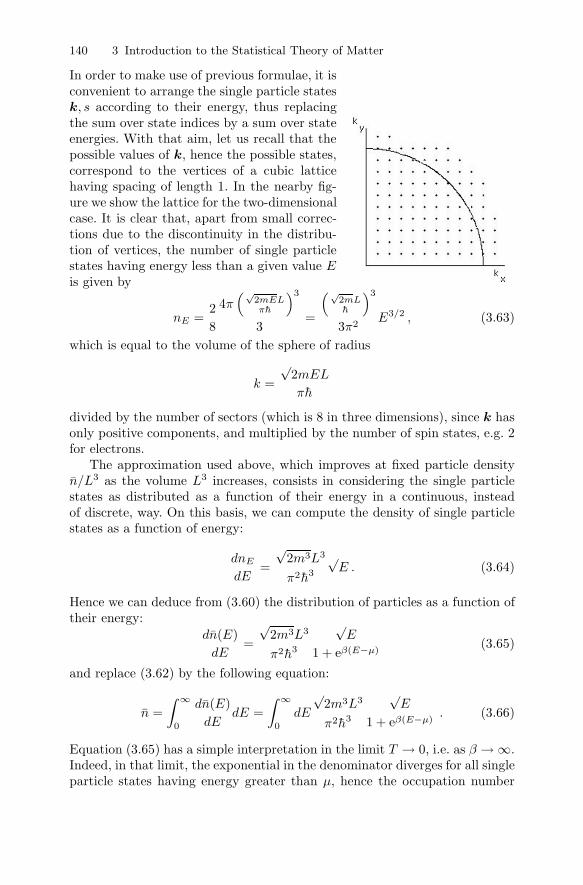
140 3 Introduction to the Statistical Theory of Matter
In order to make use of previous formulae, it isconvenient to arrange the single particle statesk, s according to their energy, thus replacingthe sum over state indices by a sum over stateenergies. With that aim, let us recall that thepossible values of k, hence the possible states,correspond to the vertices of a cubic latticehaving spacing of length 1. In the nearby fig-ure we show the lattice for the two-dimensionalcase. It is clear that, apart from small correc-tions due to the discontinuity in the distribu-tion of vertices, the number of single particlestates having energy less than a given value Eis given by
nE =2
8
4π(√
2mELπh
)3
3=
(√2mLh
)3
3π2E3/2 , (3.63)
which is equal to the volume of the sphere of radius
k =
√2mEL
πh
divided by the number of sectors (which is 8 in three dimensions), since k hasonly positive components, and multiplied by the number of spin states, e.g. 2for electrons.
The approximation used above, which improves at fixed particle densityn/L3 as the volume L3 increases, consists in considering the single particlestates as distributed as a function of their energy in a continuous, insteadof discrete, way. On this basis, we can compute the density of single particlestates as a function of energy:
dnE
dE=
√2m3L3
π2h3
√E . (3.64)
Hence we can deduce from (3.60) the distribution of particles as a function oftheir energy:
dn(E)
dE=
√2m3L3
π2h3
√E
1 + eβ(E−μ)(3.65)
and replace (3.62) by the following equation:
n =
∫ ∞
0
dn(E)
dEdE =
∫ ∞
0
dE
√2m3L3
π2h3
√E
1 + eβ(E−μ). (3.66)
Equation (3.65) has a simple interpretation in the limit T → 0, i.e. as β →∞.Indeed, in that limit, the exponential in the denominator diverges for all singleparticle states having energy greater than μ, hence the occupation number

3.4 The Grand Canonical Ensemble and the Perfect Quantum Gas 141
vanishes for those states. The exponential instead vanishes for states havingenergy less that μ, for which the occupation number is one. Therefore thechemical potential in the limit of low temperatures, which is also called Fermi
energy EF , can be computed through the equation:
nEF=
(√2mLh
)3
3π2E
3/2F = n . (3.67)
Solving for EF , we obtain:
EF = μ|T=0 =h2
2m
(3π2ρ
)2/3, (3.68)
where ρ = n/L3 is the density of particles in the gas.In order to discuss the opposite limit, in which T is very large (β → 0),
let us set z = e−βμ and rewrite (3.66) by changing the integration variable(x = βE):
n =
√2m3L3
π2h3β32
∫ ∞
0
dx
√x
1 + zex=
√2(mkT )3L3
π2h3
∫ ∞
0
dx
√x
1 + zex. (3.69)
We see from this equation that μ must tend to −∞ as T → ∞, i.e. z mustdiverge, otherwise the right-hand side in (3.69) would diverge like T 3/2, whichis a nonsense since n is fixed a priori.
Since at high temperatures z diverges, the exponential in the denominatorof (3.60) is much greater than 1, hence (3.65) can be replaced, within a goodapproximation, by
dn(E)
dE=
(√2mLh
)3
2π2z
√Ee−βE ≡ AL3
√Ee−βE . (3.70)
The constant A, hence μ, can be computed through∫ ∞
0
AL3√
Ee−βEdE = 2AL3
∫ ∞
0
x2e−βx2
dx = −2AL3 d
dβ
∫ ∞
0
e−βx2
dx
= −AL3 d
dβ
∫ ∞
−∞e−βx2
dx = −AL3 d
dβ
√π
β=
AL3
2
√π
β3= n . (3.71)
We have therefore A = 2ρ√
β3/π = eβμ√
2m3/(π2h3), confirming thatμ→ −∞ as β → 0 (μ ∼ ln β/β).
It is remarkable that in the limit under consideration, in which the distri-bution of particles according to their energy is given by:
dn(E)
dE= 2ρ
√β3
πL3√
Ee−βE , (3.72)

142 3 Introduction to the Statistical Theory of Matter
Planck’s constant has disappeared from formulae. If consequently we adoptthe classical formula for the energy of the particles, E = mv2/2, we can findthe velocity distribution corresponding to (3.70):
dn(v)
dv≡ dn(E)
dE
dE
dv= ρ
√2m3β3
πL3v2e−βmv2/2 . (3.73)
Replacing β by 1/kT , equation (3.73) reproduces the well known Maxwelldistribution for velocities, thus confirming the identification β = 1/kT madebefore.
Fig. 3.3. A plot of the Fermi–Dirac energy distribution in arbitrary units for afermion gas with EF = 10 for kT = 0, 0.25 and 12.5. Notice the for the first twovalues of kT the distribution saturates the Pauli exclusion principle limit, while forkT = 12.5 it approaches the Maxwell–Boltzmann distribution
The figure above reproduces the behavior predicted by (3.65) for three dif-ferent values of kT , and precisely for kT = 0, 0.25 and 12.5, measured in thearbitrary energy scale given in the figure, according to which EF = 10. Thetwo curves corresponding to lower temperatures show saturation for stateswith energy E < EF , in contrast with the third curve which instead repro-duces part of the Maxwell distribution and corresponds to small occupationnumbers.
Making use of (3.65) we can compute the mean energy U of the gas:
U =
∫ ∞
0
Edn(E)
dEdE =
√2m3L3
π2h3
∫ ∞
0
√E3
1 + eβ(E−μ)dE , (3.74)
obtaining, in the low temperature limit,
U =
√8m3L3
5π2h3 E5/2F =
(3n)5/3π4/3h2
10mL2=
(3n)5/3π4/3h2
10mV 2/3, (3.75)
3.4 The Grand Canonical Ensemble and the Perfect Quantum Gas 143
where V = L3 is the volume occupied by the gas. At high temperatures wehave instead:
U = 2ρ
√β3
πL3
∫ ∞
0
E3/2e−βEdE = 4ρ
√β3
πL3
∫ ∞
0
x4e−βx2
dx
=3
2n
√β3
π
√π
β5=
3
2βn ≡ 3
2nkT . (3.76)
This result reproduces what predicted by the classical kinetic theory andin particular the specific heat at constant volume for a gram atom of gas:CV = 3/2kNA ≡ 3/2R .
In order to compute the specific heat in the low temperature case, we noticefirst that, for large values of β, equation (3.66) leads, after some computations,to μ = EF −O(β−2), hence μ = EF also at the first order in T . We can derive(3.74) with respect to T , obtaining:
C = kβ2
√2m3L3
π2h3
∫ ∞
0
√E3(E − μ) eβ(E−μ)
(1 + eβ(E−μ))2dE . (3.77)
For large values of β the exponential factor in the numerator makes the con-tributions to the integral corresponding to E � μ negligible, while the expo-nential in the denominator makes negligible contributions from E � μ. Thispermits to make a Taylor expansion of the argument of the integral in (3.77).In particular, if we want to evaluate contributions of order T , taking (3.67)into account we obtain:
C � kβ2 3n
8E32
F
∫ ∞
−∞
√E3(E − EF )(
cosh β(E−EF )2
)2 dE � kβ2 3n
8
∫ ∞
−∞
(E − EF )(cosh β(E−EF )
2
)2 dE
+ kβ2 9n
16EF
∫ ∞
−∞
(E − EF )2(cosh β(E−EF )
2
)2 dE = kn9kT
2EF
∫ ∞
−∞
( x
coshx
)2
dx
= kn3π2kT
4EF, (3.78)
showing that the specific heat has a linear dependence in T at low tempera-tures.
The linear growth of the specific heat with T for low temperatures canbe easily understood in terms of the distribution of particles at low T . Inparticular we can make reference to (3.65) and to its graphical representationshown in Fig. 3.3: at low temperatures the particles occupy the lowest possibleenergy levels, thus saturating the limit imposed by Pauli’s principle. In theseconditions most of the particles cannot exchange energy with the externalenvironment, since energy exchanges of the order of kT , which are typicalat temperature T , would imply transitions of a particle to a different energy

144 3 Introduction to the Statistical Theory of Matter
level which however is already completely occupied by other particles. If werefer to the curve corresponding to kT = 0.25 in the figure, we see that onlyparticles having energies in a small interval of width kT around the Fermienergy (EF = 10 in the figure), where the occupation number rapidly goesfrom 1 to 0, can make transitions from one energy level to another, thusexchanging energy with the reservoir and giving a contribution to the specificheat, which is of the order of k for each particle. We expect therefore a specificheat which is reduced by a factor kT/EF with respect to that for the hightemperature case: this roughly reproduces the exact result given in (3.78).
Evidently we expect the results we have obtained to apply in particular tothe electrons in the conduction band of a metal. It could seem that a gas ofelectrons be far from being non-interacting, since electrons exchange repulsiveCoulomb interactions; however Coulomb forces are largely screened by theother charges present in the metallic lattice, and can therefore be neglected,at least qualitatively, at low energies. We recall that in metals there is one freeelectron for each atom, therefore, taking iron as an example, which has a massdensity ρm � 5 103 Kg/m3 and atomic weight A � 50, the electronic density is:n/V = ρm(NA/A)103 ∼ 6 1028 particles/m3. Making use of (3.68) we obtain:
EF � (10−68/1.8 10−30)(3π26 1028
)2/3J � 10−18 J � 6 eV. If we recall that
at room temperature kT � 2.5 10−2 eV, we see that the order of magnitude ofthe contribution of electrons to the specific heat is 3 10−2R per gram atom, tobe compared with 3R, which is the contribution of atoms according to Dulongand Petit. Had we not taken quantum effects into account, thus applying theequipartition principle, we would have predicted a contribution 3/2R comingfrom electrons. That gives a further confirmation of the relevance of quantumeffects for electrons in matter.
Going back to the general case, we can obtain the equation of statefor a fermionic gas by using (3.35). From the expression for the energyEi corresponding to a particular state of the gas given in (3.49) we derive∂Ei/∂V = −2Ei/3V , hence
PV =2
3U , (3.79)
which at high temperatures, where (3.76) is valid, reproduces the well knownperfect gas law. Notice that the equation of state in the form given in (3.79)is identical to that obtained in (3.33) and indeed depends only on the dis-persion relation (giving energy in terms of momentum) assumed for the freeparticlestates, i.e. the simple form and the factor 2/3 are strictly related tohaving considered the particles as non-relativistic (see Problem 3.26 for thecase of ultrarelativistic particles).
3.4.2 The Perfect Bosonic Gas
To complete our program, let us consider a gas of spinless atoms, hence ofbosons; in order to have a phenomenological reference, we shall think in par-ticular of a mono-atomic noble gas like helium. The system can be studied

3.4 The Grand Canonical Ensemble and the Perfect Quantum Gas 145
along the same lines followed for the fermionic gas, describing its possiblestates by assigning the occupation numbers of the single particle states, withthe only difference that in this case the wave function must be symmetric inits arguments (the coordinates of the various identical particles), hence thereis no limitation on the number of particles occupying a given single particlestate. The Grand Canonical partition function for a bosonic gas in a box istherefore
Ξ =∑{nk}
e−β(E{nk}−μ
∑k
nk) =∑{nk}
e−β∑
k
(h2π2
2mL2 k2−μ)nk
=∏k
( ∞∑nk=0
e−β(
h2π2
2mL2 k2−μ)
nk
)
=∏k
1
1− e−β(
h2π2
2mL2 k2−μ) , (3.80)
from which the probability of the generic state of the gas follows:
p ({nk}) =e−β∑
k
(h2π2k2
2mL2 −μ)nk
Ξ
=∏k
(e−βnk
(h2π2k2
2mL2 −μ) (
1− e−β(
h2π2k2
2mL2 −μ)))
, (3.81)
which again can be written as the product of the occupation probabilitiesrelative to each single particle state:
p (nk) = e−βnk
(h2π2k2
2mL2 −μ) (
1− e−β(
h2π2k2
2mL2 −μ))
. (3.82)
The average occupation number of the generic single particle state, k, is thus
nk =
∞∑nk=0
nk p (nk) =
(1− e
−β(
h2π2k2
2mL2 −μ)) ∞∑
n=0
n e−βn
(h2π2k2
2mL2 −μ)
=e−β(
h2π2k2
2mL2 −μ)
1− e−β(
h2π2k2
2mL2 −μ) =
1
eβ(
h2π2k2
2mL2 −μ)− 1
, (3.83)
which is known as the Bose–Einstein distribution. We deduce from last equa-tion that the chemical potential cannot be greater than the energy of theground state of a single particle, i.e.
μ ≤ 3h2π2
2mL2,
otherwise the average occupation number of that state would be negative. Inthe limit of large volumes, the ground state of a particle in a box has vanishingenergy, hence μ must be negative.

146 3 Introduction to the Statistical Theory of Matter
The exact value of the chemical potential is fixed by the relation
n =∑
k
nk =∑
k
1
eβ(
h2π2k2
2mL2 −μ)− 1
. (3.84)
For the explicit computation of μ we can make use, as in the fermionic case,of the distribution in energy, considering it approximately as a continuousfunction:
dn(E)
dE=
√m3
2
L3
π2h3
√E
eβ(E−μ) − 1. (3.85)
Notice that equation (3.85) differs from the analogous given in (3.65), whichis valid in the fermionic case, both for the sign in the denominator and for aglobal factor 1/2 which is due to the absence of the spin degree of freedom.
The continuum approximation for the distribution of the single particlestates in energy is quite rough for small energies, where only few levels arepresent. In the fermionic case, however, that is not a problem, since, due tothe Pauli exclusion principle, only a few particles can occupy those levels (2per level at most in the case of electrons), so that the contribution comingfrom the low energy region is negligible. The situation is quite different inthe bosonic case. If the chemical potential is small, the occupation number ofthe lowest energy levels can be very large, giving a great contribution to thesum in (3.84). We exclude for the time being this possibility and compute thechemical potential making use of the relation:
n =
√m3
2
L3
π2h3
∫ ∞
0
dE
√E
eβ(E−μ) − 1=
√(mkT )3
2
L3
π2h3
∫ ∞
0
dx
√x
zex − 1(3.86)
where again we have set z = e−βμ ≥ 1. Defining the gas density, ρ ≡ n/L3,equation (3.86) can be rewritten as:
∫ ∞
0
dx
√x
zex − 1= π2h3ρ
√2
(mkT )3. (3.87)
On the other hand, recalling that z ≥ 1, we obtain the following inequality:∫ ∞
0
dx
√x
zex − 1≤ 1
z
∫ ∞
0
dx
√x
ex − 1≤∫ ∞
0
dx
√x
ex − 1� 2.315 , (3.88)
which can be replaced in (3.87), giving an upper limit on the ratio ρ/T 3/2.That limit can be interpreted as follows: for temperatures lower than a certainthreshold, the continuum approximation for the energy levels cannot accountfor the distribution of all particles in the box, so that we must admit a macro-scopic contribution coming from the lowest energy states, in particular fromthe ground state. The limiting temperature can be considered as a criticaltemperature, and the continuum approximation is valid only if

3.4 The Grand Canonical Ensemble and the Perfect Quantum Gas 147
T ≥ Tc � 4.38h2ρ2/3
m k. (3.89)
As T approaches the critical temperature the chemical potential vanishes andthe occupation number of the ground state becomes comparable with n, henceof macroscopic nature. For temperatures lower than Tc the computation of thetotal number of particles shown in (3.86) must be rewritten as:
n = nf +
√m3
2
L3
π2h3
∫ ∞
0
dE
√E
eβE − 1, (3.90)
where nf refers to the particles occupying the lowest energy states, while theintegral over the continuum distribution, in which μ has been neglected, takesinto account particles occupying higher energy levels. Changing variables inthe integral we obtain:
n � nf + 2.315
√(mkT )3
2
L3
π2h3 , (3.91)
showing that, for T < Tc, nf takes macroscopic values, of the order of mag-nitude of Avogadro’s number NA.
This phenomenon is known as Bose–Einstein condensation. Actually,for the usual densities found in ordinary gasses in normal conditions, i.e.ρ � 1025 particles/m3, the critical temperature is of the order of 10−2 ◦K: forthis combination of temperature and density, interatomic forces are no morenegligible even in the case of helium, so that the perfect gas approximationdoes not apply. The situation can be completely different at very low densities,indeed Bose–Einstein condensation has been recently observed for tempera-tures of the order of 10−9 ◦K and densities of the order of 1015 particles/m3.
In the opposite situation, for temperatures much greater than Tc, the ex-ponential clearly dominates in the denominator of the continuum distributionsince, analogously to what happens for fermions at high temperatures, onecan show that z � 1. Hence the −1 term can be neglected, so that the distri-bution becomes that obtained also in the fermionic case at high temperatures,i.e. the Maxwell distribution.
3.4.3 The Photonic Gas and the Black Body Radiation
We shall consider in brief the case of an electromagnetic field in a box with“almost” completely reflecting walls: we have to give up ideal reflection inorder to allow for thermal exchanges with the reservoir. From the classicalpoint of view, the field amplitude can be decomposed in normal oscillationmodes corresponding to well defined values of the frequency and to electricand magnetic fields satisfying the well known reflection conditions on the boxsurface. The modes under consideration, apart from the two possible polar-izations of the electric field, are completely analogous to the wave functionsof a particle in a box shown in (2.101), that is:
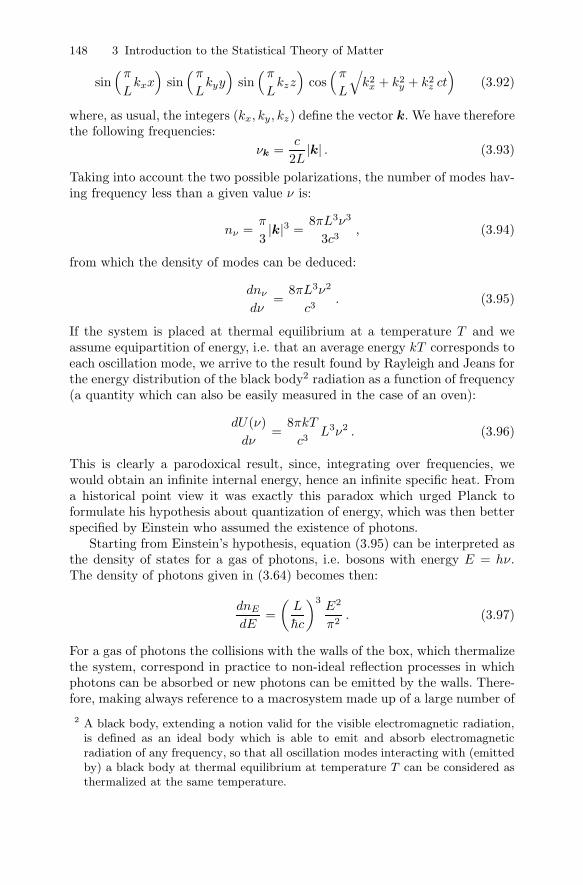
148 3 Introduction to the Statistical Theory of Matter
sin(π
Lkxx
)sin
(π
Lkyy
)sin
(π
Lkzz
)cos
(π
L
√k2
x + k2y + k2
z ct)
(3.92)
where, as usual, the integers (kx, ky, kz) define the vector k. We have thereforethe following frequencies:
νk =c
2L|k| . (3.93)
Taking into account the two possible polarizations, the number of modes hav-ing frequency less than a given value ν is:
nν =π
3|k|3 =
8πL3ν3
3c3, (3.94)
from which the density of modes can be deduced:
dnν
dν=
8πL3ν2
c3. (3.95)
If the system is placed at thermal equilibrium at a temperature T and weassume equipartition of energy, i.e. that an average energy kT corresponds toeach oscillation mode, we arrive to the result found by Rayleigh and Jeans forthe energy distribution of the black body2 radiation as a function of frequency(a quantity which can also be easily measured in the case of an oven):
dU(ν)
dν=
8πkT
c3L3ν2 . (3.96)
This is clearly a parodoxical result, since, integrating over frequencies, wewould obtain an infinite internal energy, hence an infinite specific heat. Froma historical point view it was exactly this paradox which urged Planck toformulate his hypothesis about quantization of energy, which was then betterspecified by Einstein who assumed the existence of photons.
Starting from Einstein’s hypothesis, equation (3.95) can be interpreted asthe density of states for a gas of photons, i.e. bosons with energy E = hν.The density of photons given in (3.64) becomes then:
dnE
dE=
(L
hc
)3E2
π2. (3.97)
For a gas of photons the collisions with the walls of the box, which thermalizethe system, correspond in practice to non-ideal reflection processes in whichphotons can be absorbed or new photons can be emitted by the walls. There-fore, making always reference to a macrosystem made up of a large number of
2 A black body, extending a notion valid for the visible electromagnetic radiation,is defined as an ideal body which is able to emit and absorb electromagneticradiation of any frequency, so that all oscillation modes interacting with (emittedby) a black body at thermal equilibrium at temperature T can be considered asthermalized at the same temperature.

3.4 The Grand Canonical Ensemble and the Perfect Quantum Gas 149
similar boxes, there is actually no constraint on the total number of particles,hence the chemical potential must vanish.
The distribution law of the photons in energy is then given by:
dn(E)
dE=
(L
hc
)3E2
π2
1
eE
kT − 1. (3.98)
From this law we can deduce the distribution in frequency:
dn(ν)
dν=
(L
hc
)3(hν)2
π2
h
ehνkT − 1
=8π
c3L3 ν2
ehνkT − 1
(3.99)
and we can finally write the energy distribution of the radiation as a functionof frequency by multiplying both sides of (3.99) by the energy carried by eachphoton:
dU(ν)
dν=
8πh
c3L3 ν3
ehνkT − 1
. (3.100)
This distribution was deduced for the first time by Planck and was indeednamed after him.
It is evident that at small frequencies Planck distribution is practicallyequal to that in (3.96). Instead at high frequencies energy quantization leadsto an exponential cut in the energy distribution which eliminates the paradoxof an infinite internal energy and of an infinite specific heat. We notice thatthe phenomenon suppressing the high energy modes in the computation of thespecific heat is the same leading to a vanishing specific heat for the harmonicoscillator when kT � hν (the system cannot absorb a quantity of energy lessthan the minimal quantum hν) and indeed, as we have already stressed atthe end of Section 2.7, the radiation field in a box can be considered as aninfinite collection of independent harmonic oscillators of frequencies given bythe resonant frequencies of the box.
Suggestions for Supplementary Readings
• F. Reif: Statistical Physics - Berkeley Physics Course, volume 5 (Mcgraw-HillBook Company, New York 1965)
• E. Schrodinger: Statistical Thermodynamics (Cambridge University Press, Cam-bridge 1957)
• T. L. Hill: An Introduction to Statistical Thermodynamics (Addison-Wesley Pub-lishing Company Inc., Reading 1960)
• F. Reif: Fundamentals of Statistical and Thermal Physics (Mcgraw-Hill BookCompany, New York 1965)

150 3 Introduction to the Statistical Theory of Matter
Problems
3.1. We have to place four distinct objects into 3 boxes. How many possibledifferent distributions can we choose? What is the multiplicity M of eachdistribution? And its probability p?
Answer: We can make 3 different choices for each object, therefore the total num-
ber of possible choices is 34 = 81. The total number of possible distributions is
instead given by all the possible choices of non-negative integers n1, n2, n3 with
n1 + n2 + n3 = 4, i.e. (4 + 1)(4 + 2)/2 = 15. There are in particular 3 distributions
like (4, 0, 0), each with p =M/81 = 1/81; 6 like (3, 1, 0), with p =M/81 = 4/81; 3
like (2, 2, 0), with p =M/81 = 6/81; 3 like (2, 1, 1), with p =M/81 = 12/81.
3.2. The integer number k can take values in the range between 0 and 8according to the binomial distribution:
P (k) =1
28
(8
k
).
Compute the mean value of k and its mean quadratic deviation.
Answer: k = 4 ; 〈(k − k)2〉 = 2 .
3.3. Let us consider a system which can be found in 4 possible states, enumer-ated by the index k = 0, 1, 2, 3 and with energy Ek = εk, where ε = 10−2 eV.The system is at thermal equilibrium at room temperature T � 300◦K. Whatis the probability of the system being in the highest energy state?
Answer: Z =∑3
k=0e−βεk ; U = (1/Z)
∑3
k=0εke−βεk � 1.035 10−2 eV ;
Pk=3 = (1/Z)e−3βε � 0.127.
3.4. A diatomic molecule is made up of two particles of equal mass M =10−27 Kg which are kept at a fixed distance L = 4 10−10 m. A set of N = 109
such systems, which are not interacting among themselves, is in thermal equi-librium at a temperature T = 1◦K. Estimate the number of systems whichhave a non-vanishing angular momentum (computed with respect to theircenter of mass), i.e. the number of rotating molecules, making use of the factthat the number of states with angular momentum nh is equal to 2n + 1.
Answer: If we quantize rotational energy according to Bohr, then the possible energy
levels are En = n2h2/(ML2) � 4.3 10−4n2 eV, each corresponding to 2n+1 different
states. These states are occupied according to the Canonical Distribution. The par-
tition function is Z =∑∞
n=0(2n+1)e−En/kT . If T = 1◦K, then kT � 0.862 10−4 eV,
hence e−En/kT � e−5.04n2 � (6.47 10−3)n2
. Therefore the two terms with n = 0, 1
give a very good approximation of the partition function, Z � 1 + 1.94 10−2. The
probability that a molecule has n = 0 is 1/Z, hence the number of rotating molecules
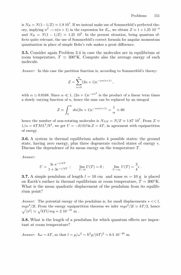
Problems 151
is NR = N(1−1/Z) � 1.9 107. If we instead make use of Sommerfeld’s perfected the-
ory, implying n2 → n(n + 1) in the expression for En, we obtain Z � 1 + 1.25 10−4
and NR = N(1 − 1/Z) � 1.25 105. In the present situation, being quantum ef-
fects quite relevant, the use of Sommerfeld’s correct formula for angular momentum
quantization in place of simple Bohr’s rule makes a great difference.
3.5. Consider again Problem 3.4 in case the molecules are in equilibrium atroom temperature, T � 300◦K. Compute also the average energy of eachmolecule.
Answer: In this case the partition function is, according to Sommerfeld’s theory:
Z =
∞∑n=0
(2n + 1)e−αn(n+1) ,
with α � 0.0168. Since α � 1, (2n + 1)e−αn2
is the product of a linear term timesa slowly varying function of n, hence the sum can be replaced by an integral
Z �∫ ∞
0
dn(2n + 1)e−αn(n+1) =1
α� 60
hence the number of non-rotating molecules is NNR = N/Z � 1.67 107. From Z �1/α = kTML2/h2, we get U = −∂/∂β ln Z = kT , in agreement with equipartition
of energy.
3.6. A system in thermal equilibrium admits 4 possible states: the groundstate, having zero energy, plus three degenerate excited states of energy ε.Discuss the dependence of its mean energy on the temperature T .
Answer:
U =3ε e−ε/kT
1 + 3e−ε/kT; lim
T→0U(T ) = 0 ; lim
T→∞U(T ) =
3
4ε .
3.7. A simple pendulum of length l = 10 cm and mass m = 10 g is placedon Earth’s surface in thermal equilibrium at room temperature, T = 300◦K.What is the mean quadratic displacement of the pendulum from its equilib-rium point?
Answer: The potential energy of the pendulum is, for small displacements s << l,
mgs2/2l. From the energy equipartition theorem we infer mgs2/2l � kT/2, hence√〈s2〉 �
√kT l/mg = 2 10−10 m .
3.8. What is the length of a pendulum for which quantum effects are impor-tant at room temperature?
Answer: hω ∼ kT , so that l = g/ω2 ∼ h2g/(kT )2 ∼ 6.5 10−28 m.
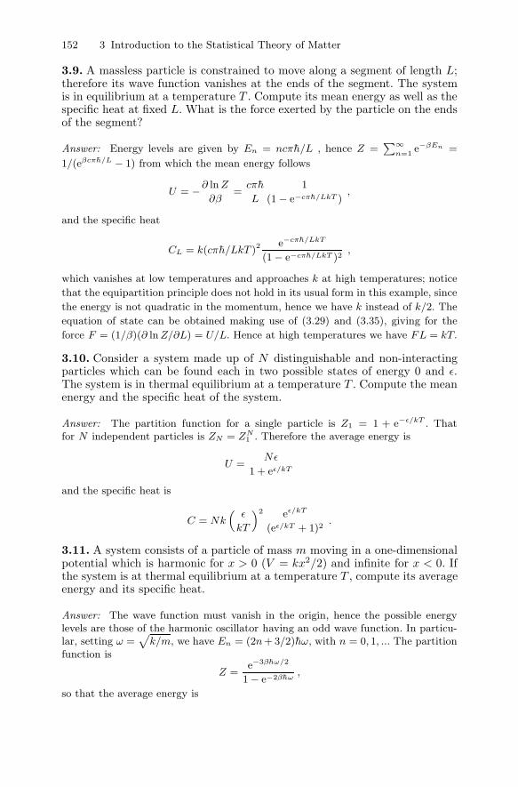
152 3 Introduction to the Statistical Theory of Matter
3.9. A massless particle is constrained to move along a segment of length L;therefore its wave function vanishes at the ends of the segment. The systemis in equilibrium at a temperature T . Compute its mean energy as well as thespecific heat at fixed L. What is the force exerted by the particle on the endsof the segment?
Answer: Energy levels are given by En = ncπh/L , hence Z =∑∞
n=1e−βEn =
1/(eβcπh/L − 1) from which the mean energy follows
U = −∂ ln Z
∂β=
cπh
L
1
(1− e−cπh/LkT ),
and the specific heat
CL = k(cπh/LkT )2e−cπh/LkT
(1− e−cπh/LkT )2,
which vanishes at low temperatures and approaches k at high temperatures; notice
that the equipartition principle does not hold in its usual form in this example, since
the energy is not quadratic in the momentum, hence we have k instead of k/2. The
equation of state can be obtained making use of (3.29) and (3.35), giving for the
force F = (1/β)(∂ ln Z/∂L) = U/L. Hence at high temperatures we have FL = kT.
3.10. Consider a system made up of N distinguishable and non-interactingparticles which can be found each in two possible states of energy 0 and ε.The system is in thermal equilibrium at a temperature T . Compute the meanenergy and the specific heat of the system.
Answer: The partition function for a single particle is Z1 = 1 + e−ε/kT . Thatfor N independent particles is ZN = ZN
1 . Therefore the average energy is
U =Nε
1 + eε/kT
and the specific heat is
C = Nk(
ε
kT
)2 eε/kT
(eε/kT + 1)2.
3.11. A system consists of a particle of mass m moving in a one-dimensionalpotential which is harmonic for x > 0 (V = kx2/2) and infinite for x < 0. Ifthe system is at thermal equilibrium at a temperature T , compute its averageenergy and its specific heat.
Answer: The wave function must vanish in the origin, hence the possible energylevels are those of the harmonic oscillator having an odd wave function. In particu-lar, setting ω =
√k/m, we have En = (2n + 3/2)hω, with n = 0, 1, ... The partition
function is
Z =e−3βhω/2
1− e−2βhω,
so that the average energy is

Problems 153
U =3hω
2+
2hω
e2βhω − 1
and the specific heat is
C = k(2βhω)2e2βhω
(e2βhω − 1)2.
3.12. Compute the average energy of a classical three-dimensional isotropicharmonic oscillator of mass m and oscillation frequency ν = 2πω in equilib-rium at temperature T .
Answer: The state of the classical system is assigned in terms of the momentump and the coordinate x of the oscillator, it is therefore represented by a point inphase space corresponding to an energy E(p, x) = p2/2m+mω2x2/2. The canonicalpartition function can therefore be written as an integral over phase space
Z =
∫d3p d3x
Δe−βp2/2me−βmω2x2/2
where Δ is an arbitrary effective volume in phase space needed to fix how we count
states (that is actually not arbitrary according to the quantum theory, which requires
Δ ∼ h3). A simple computation of Gaussian integrals gives Z = Δ−1(2π/ωβ)3, hence
U = −(∂/∂β) ln Z = 3kT , in agreement with equipartition of energy.
3.13. A particle of mass m moves in the x− y plane under the influence of ananisotropic harmonic potential V (x, y) = m(ω2
xx2/2+ω2yy
2/2), with ωy � ωx.Therefore the energy levels coincide with those of a system made up of twodistinct particles moving in two different one-dimensional harmonic potentialscorresponding respectively to ωx and ωy. The system is in thermal equilibriumat a temperature T . Compute the specific heat and discuss its behaviour as afunction of T .
Answer: The partition function is the product of the partition functions of thetwo distinct harmonic oscillators, hence the average energy and the specific heatwill be the sum of the respective quantities. In particular
C =(hωx)2
kT 2
eβhωx
(eβhωx−1)2+
(hωy)2
kT 2
eβhωy
(eβhωy−1)2.
We have three different regimes: C ∼ 0 if kT � hωy , C ∼ k if hωy � kT � hωx
and finally C ∼ 2k if kT � hωx.
3.14. Compute the mean quadratic velocity for a rarefied and ideal gas ofparticles of mass M = 10−20 Kg in equilibrium at room temperature.
Answer: According to Maxwell distribution, 〈v2〉 = 3kT/M � 1.2 m2/s2.
3.15. Taking into account that a generic molecule has two rotational degreesof freedom, compute, using the theorem of equipartition of energy, the av-erage square angular momentum J2 of a molecule whose moment of inertia

154 3 Introduction to the Statistical Theory of Matter
about the center of mass is I = 10−39 Kg m2, independently of the rotationaxis, if the temperature is T = 300 ◦K. Discuss the validity of the theorem ofequipartition of energy in the given conditions.
Answer: On account of the equipartition of energy, the average rotational kinetic
energy of the molecule is 2kT = 8.29 10−21 J = J2/2I , thus J2 = 1.66 10−59 J s.
The theorem of equipartition of energy is based on the assumption that the en-
ergy, and hence the square angular momentum, be a continuous variable, while, as
a matter of fact (see e.g. Problem 2.1), it is quantized according to the formula
J2 = n(n + 1)h2. Therefore the validity of the energy equipartition requires that
the difference between two neighboring values of J2 be much smaller than J2, i.e.
(2n + 1)/(n(n + 1)) � 2/n � 1. In the given conditions n � J/h � √1.49 109,
therefore previous inequality is satisfied.
3.16. Consider a diatomic gas, whose molecules can be described schemati-cally as a pair of pointlike particles of mass M = 10−27 Kg, which are keptat an equilibrium distance d = 2 10−10 m by an elastic force of constantK = 11.25 N/m. A quantity equal to 1.66 gram atoms of such gas is con-tained in volume V = 1 m3. Discuss the qualitative behaviour of the specificheat of the system as a function of temperature. Consider the molecules asnon-interacting and as if each were contained in a cubic box with reflectingwalls of size L3 = V/N , where N is the total number of molecules.
Answer: Three different energy scales must be considered. The effective volume
available for each molecule sets an energy scale E1 = h2π2/(4ML2) � 1.7 10−6 eV,
which is equal to the ground state energy for a particle of mass 2M in a cubic
box, corresponding to a temperature T1 = E1/k � 0.02◦K. The minimum rota-
tional energy is instead, according to Sommerfeld, E2 = h2/(Md2) � 3.5 10−3 eV,
corresponding to a temperature T2 = E2/k � 40◦K. Finally, the fundamental os-
cillation energy is E3 = h√
2K/M � 0.098 eV, corresponding to a temperature
T3 = E2/k � 1140◦K. For T1 � T � T2 the system can be described as a classical
perfect gas of pointlike particles, since rotational and vibrational modes are not yet
excited, hence the specific heat per molecule is C ∼ 3k/2. For T2 � T � T3 the
system can be described as a classical perfect gas of rigid rotators, hence C ∼ 5k/2.
Finally, for T � T3 also the (one-dimensional) vibrational mode is excited and
C ∼ 7k/2. This roughly reproduces, from a qualitative point of view and with an
appropriate rescaling of parameters, the observed behavior of real diatomic gasses.
3.17. We have a total mass M = 10−6 Kg of a dust of particles of massm = 10−17 Kg. The dust particles can move in the vertical x − z semi-planedefined by x > 0, and above a line forming an angle α, with tanα = 10−3,with the positive x axis. The dust is in thermal equilibrium in air at roomtemperature (T = 300 ◦K) and hence the particles, which do not interactamong themselves, have planar Brownian motion above the mentioned line.What is the distribution of particles along the positive x axis and which theiraverage distance x from the vertical z axis?

Problems 155
Answer: We start assuming that, in the mentioned conditions, quantum effectsare negligible and hence the particle distribution in the velocity and position planeis given by the Maxwell-Boltzmann law: d4n/((d2v)dxdz) = N exp(−E/kT ) =N exp(−(mv2/2 + mgz)/(kT )) where g is the gravitational acceleration and N is anormalization factor. Then the x-distribution of particles is given by:
dn
dx=
∫ ∞
−∞dvx
∫ ∞
−∞dvy
∫ ∞
x tan α
dzd4n
d2vdxdz
=2πkTN
m
∫ ∞
x tan α
dze−mgz/(kT ) =2π(kT )2N
m2ge−mgx tan α/(kT ) .
We can compute N using∫∞0
(dn/dx)dx = 2π(kT )3N/(tan α m3g2) = M/m = 1011
and x = kT/(mg tan α) � 4.22 10−2 m. Now we discuss the validity of the classical
approximation. The average inter-particle distance is of the order of magnitude of
mx/M ∼ 4 10−13 m, which should be much larger than the average de Broglie wave
length of the particles, which is of the order of magnitude of h/√
2mkT ∼ 2 10−15 m.
We conclude that the classical approximation is valid.
3.18. The possible stationary states of a system are distributed in energy asfollows:
d n
dE= αE3eE/E0
where E0 is some given energy scale. Compute the average energy and thespecific heat of the system for temperatures T < E0/k, then discuss the pos-sibility of reaching thermal equilibrium at T = E0/k.
Answer: Let us set β0 = 1/E0. The density of states diverges exponentially withenergy and the partition function of the system is finite only if the temperature islow enough in order for the Boltzmann factor, which instead decreases exponentiallywith energy, to be dominant at high energies. For T < E0/k (β > β0) we have:
Z =
∫ ∞
0
dEαE3e−(β−β0)E =6α
(β − β0)4
from which the internal energy U and the specific heat C = dU/dT easily follow:
U =4
β − β0=
4kTE0
E0 − kT; C =
4kE20
(E0 − kT )2.
The specific heat diverges at T = E0/k: in general that may happen in presence
of a phase transition, but in this specific case also the internal energy diverges as
T → E0/k, meaning that an infinite amount of energy must be spent in order to
bring the system at equilibrium at that temperature, i.e. it is not possible to reach
thermal equilibrium at that temperature.
3.19. Consider a system made up of two identical fermionic particles whichcan occupy 4 different states. Enumerate all the possible choices for the occu-pation numbers of the single particle states. Assuming that the 4 states have

156 3 Introduction to the Statistical Theory of Matter
the following energies: E1 = E2 = 0 and E3 = E4 = ε and that the systemis in thermal equilibrium at a temperature T , compute the mean occupationnumber of one of the first two states as a function of temperature.
Answer: There are six different possible states for the whole system characterizedby the following occupation numbers (n1, n2, n3, n4) for the single particle states:(1, 1, 0, 0), (1, 0, 1, 0), (1, 0, 0, 1), (0, 1, 1, 0), (0, 1, 0, 1), (0, 0, 1, 1). The correspondingenergies are 0, ε, ε, ε, ε, 2ε. The mean occupation number of the first single particlestate (i.e. 〈n1〉) is then given by averaging the value of n1 over the 6 possible statesweighted using the Canonical Distribution, i.e.
〈n1〉 =(1 + 2e−βε)
(1 + 4e−βε + e−2βε).
3.20. A system, characterized by 3 different single particle states, is filledwith 4 identical bosons. Enumerate the possible states of the system specify-ing the corresponding occupation numbers. Discuss also the case of 4 identicalfermions.
Answer: The possible states can be enumerated by indicating all possible choices
for the occupation numbers n1, n2, n3 satisfying n1 + n2 + n3 = 4. That leads to 15
different states. In the case of fermions, since ni = 0, 1, the constraint on the total
number of particles cannot be satisfied and there is actually no possible state of the
system.
3.21. A system, characterized by two single particle states of energy E1 = 0and E2 = ε, is filled with 4 identical bosons. Enumerate all possible choicesfor the occupation numbers. Assuming that the system is in thermal contactwith a reservoir at temperature T and that e−βε = 1
2 , compute the probabilityof all particles being in the ground state. Compare the answer with that fordistinguishable particles.
Answer: Since the occupation numbers must satisfy N1 + N2 = 4, the possi-
ble states are identified by the value of, for instance, N2, in the case of bosons
(N2 = 0, 1, 2, 3, 4), and have energy εN2. In the case of distinguishable particles
there are instead 4!/(N2!(4−N2)!) different states for each value of N2. The prob-
ability of all the particles being in the ground state is 16/31 in the first case and
(2/3)4 in the second case: notice that this probability is highly enhanced in the case
of bosons.
3.22. Consider a gas of electrons at zero temperature. What is density atwhich relativistic effects show up? Specify the answer by finding the densityfor which electrons occupy states corresponding to velocities v =
√3 c/2.
Answer: At T = 0 electrons occupy all levels below the Fermi energy EF , orequivalently below the corresponding Fermi momentum pF . To answer the questionwe must impose that
pF =mev√
1− v2/c2=√
3 mec .

Problems 157
On the other hand, the number of states below the Fermi momentum, assuming thegas is contained in a cubic box of size L, is
N =p3
F L3
3h3π2,
hence ρ = p3F /(3π2h3) � 3.04 1036 particles/m3.
3.23. The density of states as a function of energy in the case of free electronsis given in (3.64). However in a conduction band the distribution may have adifferent dependence on energy. Let us consider for instance the simple casein which the density is constant, dnE/dE = γ V , where γ = 8 1047 m−3 J−1,the energy varies from zero to E0 = 1 eV and the electronic density isρ ≡ n/V = 6 1028 m−3. For T not much greater than room temperatureit is possible to assume that the bands above the conduction one are com-pletely free, while those below are completely occupied, hence the thermalproperties can be studied solely on the basis of its conduction band. Underthese assumptions, compute how the chemical potential μ depends on tem-perature.
Answer: The average total number of particles comes out to be N =∫ E0
0n(ε)g(ε)dε .
The density of levels is g(ε) = dnE/dE = γ V and the average occupation numberis n(ε) = 1/(eβ(ε−μ) + 1). After computing the integral and solving for μ we obtain
μ = kT ln
(eρ/(γkT ) − 1
1− eρ/(γkT )e−E0/kT
).
It can be verified that, since by assumption ρ/γ < E0, in the limit T → 0 μ is
equal to the Fermi energy EF = ρ/γ. Instead, in the opposite large temperature
limit, μ → −kT ln(1 − γE0/ρ), hence the distribution of electrons in energy would
be constant over the band and simply given by n(ε)g(ε) = ρV/E0, but of course in
this limit we cannot neglect the presence of other bands. Notice also that in this
case, due to the different distribution of levels in energy, we have μ→ +∞, instead
of μ → −∞, as T →∞.
3.24. The modern theory of cosmogenesis suggests that cosmic space containabout 108 neutrinos per cubic meter and for each species of these particles.Neutrinos can be considered, in a first approximation, as massless fermionshaving a single spin state instead of two, as for electrons; they belong to 6different species. Assuming that each species be independent of the others,compute the corresponding Fermi energy.
Answer: Considering a gas of neutrinos placed in a cubic box of size L, the number
of single particle states with energy below the Fermi energy EF is given, for massless
particles, by NEF = (π/6)E3F L3/(πhc)3. Putting that equal to the average number
of particles in the box, N = ρL3, we have EF = hc (6π2ρ)1/3 � 3.38 10−4 eV.
3.25. Suppose now that neutrinos must be described as particles of massmν = 0. Consider again Problem 3.24 and give the exact relativistic formula
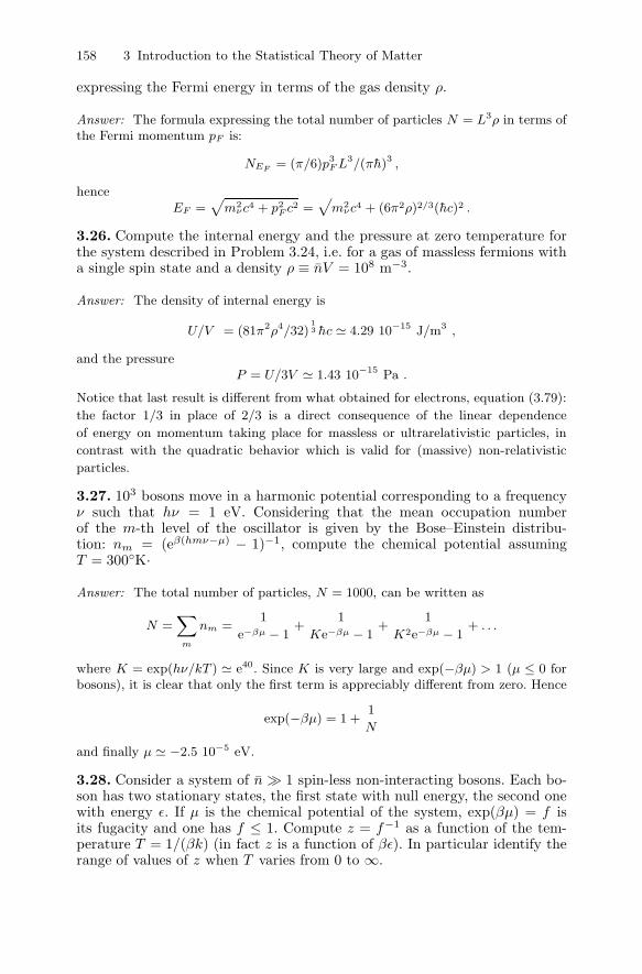
158 3 Introduction to the Statistical Theory of Matter
expressing the Fermi energy in terms of the gas density ρ.
Answer: The formula expressing the total number of particles N = L3ρ in terms ofthe Fermi momentum pF is:
NEF = (π/6)p3F L3/(πh)3 ,
henceEF =
√m2
νc4 + p2F c2 =
√m2
νc4 + (6π2ρ)2/3(hc)2 .
3.26. Compute the internal energy and the pressure at zero temperature forthe system described in Problem 3.24, i.e. for a gas of massless fermions witha single spin state and a density ρ ≡ nV = 108 m−3.
Answer: The density of internal energy is
U/V = (81π2ρ4/32)13 hc � 4.29 10−15 J/m3 ,
and the pressureP = U/3V � 1.43 10−15 Pa .
Notice that last result is different from what obtained for electrons, equation (3.79):
the factor 1/3 in place of 2/3 is a direct consequence of the linear dependence
of energy on momentum taking place for massless or ultrarelativistic particles, in
contrast with the quadratic behavior which is valid for (massive) non-relativistic
particles.
3.27. 103 bosons move in a harmonic potential corresponding to a frequencyν such that hν = 1 eV. Considering that the mean occupation numberof the m-th level of the oscillator is given by the Bose–Einstein distribu-tion: nm = (eβ(hmν−μ) − 1)−1, compute the chemical potential assumingT = 300◦K·
Answer: The total number of particles, N = 1000, can be written as
N =∑m
nm =1
e−βμ − 1+
1
Ke−βμ − 1+
1
K2e−βμ − 1+ . . .
where K = exp(hν/kT ) � e40. Since K is very large and exp(−βμ) > 1 (μ ≤ 0 forbosons), it is clear that only the first term is appreciably different from zero. Hence
exp(−βμ) = 1 +1
N
and finally μ � −2.5 10−5 eV.
3.28. Consider a system of n � 1 spin-less non-interacting bosons. Each bo-son has two stationary states, the first state with null energy, the second onewith energy ε. If μ is the chemical potential of the system, exp(βμ) = f isits fugacity and one has f ≤ 1. Compute z = f−1 as a function of the tem-perature T = 1/(βk) (in fact z is a function of βε). In particular identify therange of values of z when T varies from 0 to ∞.

Problems 159
Answer: It is convenient to study ζ ≡ z exp(βε/2) instead of z. ζ must divergein the T → 0 limit since z ≥ 1. The condition that the sum of state occupationnumbers be equal to n gives the equation:
ζ2 − 2 cosh(βε/2)(1 + 1/n)ζ + 2/n + 1 = 0 ,
whose solutions are
ζ± = cosh(βε/2)(1 + 1/n)±√
cosh2(βε/2)(1 + 1/n)2 − 2/n− 1] .
One must choose ζ+ since ζ− vanishes in the T → 0 limit. Then one has in the
T → 0 limit ζ → 2 cosh(βε/2)(1+1/n)→ exp(βε/2)(1+1/n) and hence the average
occupation number of the zero energy state n0 = 1/(ζ exp(−βε/2)− 1) → n. In the
T → ∞ limit one has ζ → 1 + 2/n and hence n0 → 2/n. Therefore z ranges from
1 + 1/n to 1 + 2/n and the chemical potential ranges approximately from −kT/n,
fot T small, to −2kT/n for T large. There is no Bose condensation.
3.29. A system is made up of N identical bosonic particles of mass m mov-ing in a one-dimensional harmonic potential V (x) = mω2x2/2. What is thedistribution of occupation numbers corresponding to the ground state of thesystem? And that corresponding to the first excited state? Determine theenergy of both states.
If hω = 0.1 eV and if the system is in thermal equilibrium at room tem-perature, T = 300◦K, what is the ratio R of the probability of the systembeing in the first excited state to that of being in the fundamental one? Howthe last answer changes in case of distinguishable particles?
Answer: In the ground state all particles occupy the single particle state of low-
est energy hω/2, hence E = Nhω/2, while in the first excited state one of the N
particles has energy 3hω/2, hence E = (N + 2)hω/2. The ground state has degen-
eracy 1 both for identical and distinguishable particles. The first excited state has
denegeracy 1 in the case of bosons while the degeneracy is N in the other case,
since it makes sense to ask which of the N particles has energy 3hω/2. Therefore
R = e−hω/kT � 0.021 for bosons and R � N 0.021 in the second case. For large N
the probability of the system being excited is much suppressed in the case of bosons
with respect to the case of distinguishable particles.
3.30. Consider again Problem 3.29 in the case of fermions having a single spinstate and for hω = 1 eV and T � 1000◦K.
Answer: In the ground state of the system the first N levels of the harmonic os-
cillator are occupied, hence its energy is E0 =∑N−1
i=0(n + 1/2)hω = (N2/2)hω.
The minimum possible excitation of this state corresponds to moving the fermion of
highest energy up to the next free level, hence the energy of the first excited state
is E1 = E0 + hω. The ratio R is equal to e−hω/kT = 9.12 10−6.
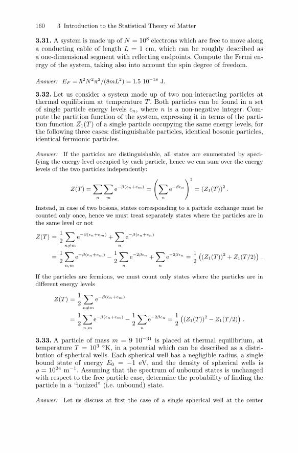
160 3 Introduction to the Statistical Theory of Matter
3.31. A system is made up of N = 108 electrons which are free to move alonga conducting cable of length L = 1 cm, which can be roughly described asa one-dimensional segment with reflecting endpoints. Compute the Fermi en-ergy of the system, taking also into account the spin degree of freedom.
Answer: EF = h2N2π2/(8mL2) = 1.5 10−18 J.
3.32. Let us consider a system made up of two non-interacting particles atthermal equilibrium at temperature T . Both particles can be found in a setof single particle energy levels εn, where n is a non-negative integer. Com-pute the partition function of the system, expressing it in terms of the parti-tion function Z1(T ) of a single particle occupying the same energy levels, forthe following three cases: distinguishable particles, identical bosonic particles,identical fermionic particles.
Answer: If the particles are distinguishable, all states are enumerated by speci-fying the energy level occupied by each particle, hence we can sum over the energylevels of the two particles independently:
Z(T ) =∑
n
∑m
e−β(εn+em) =
(∑n
e−βεn
)2
= (Z1(T ))2 .
Instead, in case of two bosons, states corresponding to a particle exchange must becounted only once, hence we must treat separately states where the particles are inthe same level or not
Z(T ) =1
2
∑n�=m
e−β(εn+em) +∑
n
e−β(εn+en)
=1
2
∑n,m
e−β(εn+em) − 1
2
∑n
e−2βεn +∑
n
e−2βεn =1
2
((Z1(T ))2 + Z1(T/2)
).
If the particles are fermions, we must count only states where the particles are indifferent energy levels
Z(T ) =1
2
∑n�=m
e−β(εn+em)
=1
2
∑n,m
e−β(εn+em) − 1
2
∑n
e−2βεn =1
2
((Z1(T ))2 − Z1(T/2)
).
3.33. A particle of mass m = 9 10−31 is placed at thermal equilibrium, attemperature T = 103 ◦K, in a potential which can be described as a distri-bution of spherical wells. Each spherical well has a negligible radius, a singlebound state of energy E0 = −1 eV, and the density of spherical wells isρ = 1024 m−1. Assuming that the spectrum of unbound states is unchangedwith respect to the free particle case, determine the probability of finding theparticle in a “ionized” (i.e. unbound) state.
Answer: Let us discuss at first the case of a single spherical well at the center
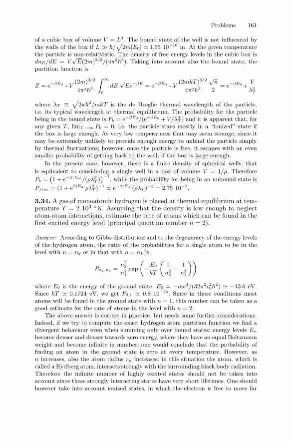
Problems 161
of a cubic box of volume V = L3. The bound state of the well is not influenced bythe walls of the box if L � h/
√2m|E0| � 1.55 10−10 m. At the given temperature
the particle is non-relativistic. The density of free energy levels in the cubic box isdnE/dE = V
√E(2m)3/2/(4π2h3). Taking into account also the bound state, the
partition function is
Z = e−βE0 +V(2m)3/2
4π2h3
∫ ∞
0
dE√
Ee−βE = e−βE0 +V(2mkT )3/2
4π2h3
√π
2= e−βE0 +
V
λ3T
where λT ≡√
2πh2/mkT is the de Broglie thermal wavelength of the particle,i.e. its typical wavelength at thermal equilibrium. The probability for the particlebeing in the bound state is Pb = e−βE0/(e−βE0 +V/λ3
T ) and it is apparent that, forany given T , limV →∞ Pb = 0, i.e. the particle stays mostly in a “ionized” state ifthe box is large enough. At very low temperatures that may seem strange, since itmay be extremely unlikely to provide enough energy to unbind the particle simplyby thermal fluctuations; however, once the particle is free, it escapes with an evensmaller probability of getting back to the well, if the box is large enough.
In the present case, however, there is a finite density of spherical wells: that
is equivalent to considering a single well in a box of volume V = 1/ρ. Therefore
Pb =(1 + e−β|E0|/(ρλ3
T ))−1
, while the probability for being in an unbound state is
Pfree = (1 + eβ|E0|ρλ3T )−1 � e−β|E0|(ρλT )−3 = 2.75 10−2.
3.34. A gas of monoatomic hydrogen is placed at thermal equilibrium at tem-perature T = 2 103 ◦K. Assuming that the density is low enough to neglectatom-atom interactions, estimate the rate of atoms which can be found in thefirst excited energy level (principal quantum number n = 2).
Answer: According to Gibbs distribution and to the degeneracy of the energy levelsof the hydrogen atom, the ratio of the probabilities for a single atom to be in thelevel with n = n2 or in that with n = n1 is
Pn2,n1 =n2
2
n21
exp
(−E0
kT
(1
n22
− 1
n21
))
where E0 is the energy of the ground state, E0 = −me4/(32π2ε20h2) � −13.6 eV.
Since kT � 0.1724 eV, we get P2,1 � 0.8 10−24. Since in those conditions mostatoms will be found in the ground state with n = 1, this number can be taken as agood estimate for the rate of atoms in the level with n = 2.
The above answer is correct in practice, but needs some further considerations.Indeed, if we try to compute the exact hydrogen atom partition function we find adivergent behaviour even when summing only over bound states: energy levels En
become denser and denser towards zero energy, where they have an equal Boltzmannweight and become infinite in number: one would conclude that the probability offinding an atom in the ground state is zero at every temperature. However, asn increases, also the atom radius rn increases: in this situation the atom, which iscalled a Rydberg atom, interacts strongly with the surrounding black body radiation.Therefore the infinite number of highly excited states should not be taken intoaccount since these strongly interacting states have very short lifetimes. One shouldhowever take into account ionized states, in which the electron is free to move far

162 3 Introduction to the Statistical Theory of Matter
away from the binding proton. Concerning the statistical weight of these states, wecan make reference to Problem (3.33): following a similar argument we realize thationized states become statistically relevant, with respect to the ground state, when
the density of atoms is of the order of e−β|E0|/λ3T = e−β|E0| (mkT/(2πh2)
)3/2 ∼e−β|E0|1028 m−3 ∼ 10−6 m−3 .
3.35. Consider a homogeneous gas of non-interacting, non-relativistic bosons,which are constrained to move freely on a plane surface. Compute the rela-tion linking the density ρ, the temperature T and the chemical potential μ ofthe system. Does Bose-Einstein condensation occur? Does the answer to thelast question change if an isotropic harmonic potential acts in the directionsparallel to the surface?
Answer: An easy computation shows that the density of states for free particlesin two dimensions is independent of the energy and given by
dnE
dE=
mA
2πh2
where m is the particle mass and A is the total area of the surface. According toBose-Einstein distribution, the total particle density is then given by:
ρ =N
A=
m
2πh2
∫ ∞
0
dE1
e(E−μ)/(kT ) − 1= −kTm
2πh2ln(1− eμ/(kT )
).
The chemical potential turns out to be negative, as expected. It is interesting toconsider the limit of low densities, in which the typical inter-particle distance ismuch greater than the typical thermal de Broglie wavelength (ρ−1/2 � h/
√mkT )
and
μ � kT ln
(2πh2ρ
mkT
),
while in the opposite case of high densities one obtains
μ = −kT exp
(−2πh2ρ
mkT
).
At variance with the three-dimensional case, ρ diverges as μ → 0, meaning thatthe system can account for an arbitrarily large number of particles, with no needfor a macroscopic number of particles in the ground state, therefore Bose-Einsteincondensation does not occur in two dimensions, due to the different density of states.
If the system is placed in a two-dimensional isotropic harmonic potential ofangular frequency ω, the energy levels are En = hω(n+1), with degeneracy n+1, sothat the total number of energy levels found below a given energy E is ∼ E2/(2h2ω2)and the density of states becomes dnE/dE � E/(h2ω2). The average number ofparticles (the system is not homogeneous and we cannot define a density) is
N =1
h2ω2
∫ ∞
0
dEE
e(E−μ)/(kT ) − 1=
k2T 2
h2ω2
∫ ∞
−μ/(kT )
dxx + μ/(kT )
ex − 1.
In this case the integral in the last member stays finite even in the limit μ → 0,
meaning that condensation in the ground state is necessary to allow for an arbitrary
average number of particles N . The condensation temperature is Tc ∼√
Nhω/k
and goes to zero, at fixed N , as ω → 0 (i.e. going back to the free case).

Problems 163
3.36. A system of massless particles at thermal equilibrium is characterizedby the known equation of state U/V − 3P = 0, linking the pressure P tothe density of internal energy U/V . For a homogeneous system of spinless,non-interacting and distinguishable particles of density ρ, placed at thermalequilibrium at temperature T , compute the lowest order violation to the aboverelation due to a non-zero particle mass m.
Answer: For one particle in a cubic box of volume V = L3, energy levels are
written as E =√
p2c2 + m2c4 =√
m2c4 + (π2h2c2/L2)(n2x + n2
y + n2z), with nx,
ny and nz positive integers. The number of energy levels below a given threshold
E =√
p2c2 + m2c4 is given by p3V/(3π2h3), from which one obtains the density ofstates dnE/dE = V pE/(c2h2h3). The derivative of one energy level with respect tothe volume is ∂E/∂V = p2c2/(3V E).
The internal energy and the pressure are given, for a single particle, by
U =
∫∞mc2
dE(dnE/dE)e−βEE∫∞mc2
dE(dnE/dE)e−βE; P =
∫∞mc2
dE(dnE/dE)e−βE(∂E/∂V )∫∞mc2
dE(dnE/dE)e−βE
so that
U−3PV =
∫∞mc2
dE(dnE/dE)e−βE(E − p2c2/E)∫∞mc2
dE(dnE/dE)e−βE=
m2c4∫∞
mc2dE(dnE/dE)e−βE/E∫∞
mc2dE(dnE/dE)e−βE
.
To keep the lowest order in m it is sufficient to evaluate the integrals in the lastexpression in the limit m = 0. Finally, multiplying for the total number of particlesin the box, N = ρV , we get
U
V− 3P =
ρ m2c4
2kT.
This is the first term of an expansion in terms of the parameter mc2/kT .
3.37. Consider a rarefied gas of particles of mass m in equilibrium at tem-perature T . The probability distribution of particle velocities is given by theGaussian Maxwell-Boltzmann (MB) formula
p(v) d3v =( m
2πkT
)3/2
e−mv2/(2kT )d3v .
Considering a pair of particles in the gas, labelled by 1 and 2, compute thedistribution of the relative velocities vR ≡ v1 − v2, and that of the velocityof their center of mass vB ≡ (v1 + v2)/2.
Answer: The particles in the chosen pair behave as independent systems, hencethe probability density in the six-dimensional (v1, v2) space is just the product ofthe two densities:
p(v1, v2)d3v1d
3v2 =(
m
2πkT
)3
e−m(v21+v2
2)/(2kT )d3v1d3v2 .
If we change variables passing from (v1, v2) to (vR, vB), the new probability densityis given by

164 3 Introduction to the Statistical Theory of Matter
p(vR, vB)d3vRd3vB = p(v1, v2)d3v1d
3v2
hence p(vR, vB) = J(vR, vB)p(v1, v2) where J is the Jacobian matrix, that is, theabsolute value of the determinant of the six-dimensional matrix whose elements are∂vi
a/∂vjS where a is either 1 or 2 and S is either R or B and i, j label the Cartesian
components. Furthermore p(v1, v2) must be considered a function of (vR, vB). It issoon verified that J = 1 and that v2
1 + v22 = (1/2)v2
R + 2v2B . Therefore we have
p(vR, vB)d3vRd3vB =(
μ
2πkT
)3/2
e−μv2R
/(2kT )(
M
2πkT
)3/2
e−Mv2B
/(2kT )
where μ = m/2 is the reduced mass of the pair of particles and M = 2m is theirtotal mass.
Then we see that our result corresponds to the product of the MB distribution
of a single particle of mass μ and velocity vR and that of a single particle of mass M
and velocity vB . If we search for the vR distribution of the pair, we must integrate
over vB and we get the first MB distribution, corresponding to the mass μ. If
instead we search for the vB distribution of the pair, we must integrate over vR and
we get the second MB distribution, corresponding to the mass M . It can be easily
verified that the result extends unchanged to the case in which the two particles
have different masses m1 and m2, defining as usual M = m1 + m2, μ = m1m2/M ,
vB = (m1v1 + m2v2)/M , vR = v1 − v2.
3.38. We have a rarefied gas of electrons for which mc2 = 0.511 MeV, inthermal equilibrium at kT = 5 103 eV. Since kT/mc2 � 1, the rarefied gas innon-relativistic. Therefore the particle momentum p distribution is given bythe Maxwell-Boltzmann formula
dPdp
=
(1
2πmkT
)3/2
e−p2/(2mkT ) .
The electron gas is mixed with a rarefied positron gas in thermal equilibriumat the same temperature. Positrons are anti-particles of electrons, therefore apositron-electron collision can produce an annihilation into two photons andhence the two gas mixture is a photon source. We would like to compute thephoton energy (frequency) distribution.
Answer: If a non-relativistic positron annihilates with a non-relativistic elec-tron and their relative momentum is p while the center of mass one is P , for-getting relativistic corrections, we find that the energy of a produced photon isE = (mc2 + p2/(2m))(1 + Pz/Mc) where we have chosen the z-axis parallel to themomentum of the photon and the second factor is the transformation factor from thecenter of mass to the laboratory frame, that is, it accounts for the non-relativisticDoppler effect. As shown in the preceding problem, considering a generic electron-positron pair, one has the center of mass P and relative momentum p distributiond6P/(dP dp) = 1/(2πmkT )3 exp(−p2/(mkT )) exp(−P 2/(4mkT )). Changing the Pz
variable into E and integrating over Px and Py we get (the only non-trivial elementof the Jacobian matrix is ∂Pz/∂E):
d4PdpdE
=2m2c
(2m2c2 + p2)(πmkT )2e−p2/(mkT ) exp
(−4m3c2(E −mc2 − p2/(2m))2
(2m2c2 + p2)2kT
)

Problems 165
which should be integrated over p. The Gaussian factor in p correesponds to a meansquare value p2 = 3mkT/2 and the standard deviation Δ2
p2 = 3(mkT )2/2. Since in
the above distribution, the Gaussian factor put apart, p2 appears only in the linearcombination mc2+p2/(2m) and since mc2 = 0.511 MeV � 3kT/4 we can replace thelinear combination with mc2 + 3kT/4 getting the final photon energy distribution:
dPdE
=1√
πmc2kT (1 + 3kT/(4mc2))exp
[− (E −mc2 − 3kT/4)2
mc2kT (1 + 3kT/(4mc2))2
].
Notice that, however exponentially decaying, the distribution does not vanish for
negative E values, this is due that for these values the non relativistic Doppler
formula does not apply. Thus negative E values should not be considered. Notice
also that, while the most probable E value is shifted by a factor 3kT/(4mc2) ∼ 10−2,
the width of the distribution is proportional to√
mc2kT , allowing for fluctuations
in E of the order of√
kT/mc2 ∼ 10%, i.e. much larger than the shift. The physical
origin of the shift is mostly in the fact that the annihilating pair has an average
energy, in the center of mass, which is larger than 2mc2, due to thermal motion, by
an amount ∼ p2/m ∼ kT . The broad distribution of energy is instead mostly due to
Doppler effect, due to the transformation from the center of mass to the laboratory
frame (see also Problem 1.27), and the broadening is proportional to the typical
center of mass velocity, which is of the order of c√
kT/mc2.
A
Quadrivectors
A concise description of Lorentz transformations and of their action on phys-ical observables can be given in terms of matrix algebra. The coordinates ofa space-time event in the reference frame O are identified with the elementsof a column matrix ξ:
ξ ≡
⎛⎜⎝
ctxyz
⎞⎟⎠ , (A.1)
while Lorentz transformations from O to a new reference frame O′, which aregiven in (1.13) and (1.14), are associated with a matrix
Λ ≡
⎛⎜⎜⎜⎝
1√1− v2
c2
0 0 −v
c√
1− v2
c2
0 1 0 00 0 1 0−v
c√
1− v2
c2
0 0 1√1− v2
c2
⎞⎟⎟⎟⎠ (A.2)
defined so that the column matrix corresponding to the coordinates of thesame space-time event in frame O′ is given by:
ξ′ ≡
⎛⎜⎝
ct′
x′
y′
z′
⎞⎟⎠ = Λξ ≡
⎛⎜⎜⎜⎝
1√1− v2
c2
0 0 −v
c√
1− v2
c2
0 1 0 00 0 1 0−v
c√
1− v2
c2
0 0 1√1− v2
c2
⎞⎟⎟⎟⎠⎛⎜⎝
ctxyz
⎞⎟⎠ . (A.3)
The products above are intended to be row by column products. To be morespecific, indicating by ai,j , with i = 1, . . . , M and j = 1, . . . , N , the elementcorresponding to the i-th row and the j-th column of the M × N matrix A(i.e. A has M rows and N columns), and by bl,m the element of the i-th rowand the j-th column of the N × P matrix B, the product AB is a M × Pmatrix whose generic element is given by:
168 A Quadrivectors
(AB)i,m =
N∑j=1
ai,jbj,m . (A.4)
As we have discussed in Chapter 2, a generic Lorentz transformation cor-responds to a homogeneous linear transformations of the event coordinateswhich leaves invariant the following quadratic form:
ξ2 ≡ x2 + y2 + z2 − c2t2 ; (A.5)
moreover, the direction of time (time arrow) is the same in both frames andif the spatial Cartesian coordinates in O are right(left)-handed, they will beright(left)-handed also in O′. In matrix algebra, the quadratic form can beeasily built up by introducing the metric
g ≡
⎛⎜⎝−1 0 0 00 1 0 00 0 1 00 0 0 1
⎞⎟⎠ , (A.6)
and defining:
ξ2 = ξT g ξ ≡ ( ct′ x′ y′ z′ )
⎛⎜⎝−1 0 0 00 1 0 00 0 1 00 0 0 1
⎞⎟⎠⎛⎜⎝
ctxyz
⎞⎟⎠ , (A.7)
where the products are still intended to be row by column.The symbol T used in the left-hand side stands for transposition, i.e. the
operation corresponding to exchanging rows with columns. Notice that, main-taining the row by column convention for matrix product, the transpose ofthe product of two matrices is the inverted product of the transposes:
(AB)T = BT AT . (A.8)
The condition that Lorentz transformations leave the quadratic form in (A.7)invariant can be now expressed as a simple matrix equation for the generictransformation Λ:
ξ′T g ξ′ = ξT ΛT gΛ ξ ≡ ξT g ξ ∀ ξ =⇒ ΛT gΛ = g . (A.9)
The additional requirements are that the determinant of Λ be one and thatits first diagonal element (i.e. first row, first column) be positive.
Equation (A.9) can be put in a different form by making use of the evidentrelation g2 = I, where I is the identity matrix (its element (i, j) is equal to1 if i = j, to 0 if i = j and of course AI = IA = A for every matrix A).Multiplying both sides of last equation in (A.9) by g on the left, we obtain:
gΛT g Λ = I =⇒ gΛT g = Λ−1 , (A.10)

A Quadrivectors 169
where the inverse matrix A−1 of a generic matrix A is defined by the equationA−1A = AA−1 = I.
Column vectors in relativity are called quadrivectors. Some specificationsabout the action of Lorentz transformations over them are however stillneeded. Let us consider a function f(ξ) depending on the space-time event ξ,which we suppose to have continuous derivatives and to be Lorentz invariant,i.e. such that f(Λξ) = f(ξ). The partial derivatives of f with respect to thecoordinates of the event form a column vector:
∂f(ξ) ≡
⎛⎜⎜⎜⎝
∂f(ξ)∂ct
∂f(ξ)∂x
∂f(ξ)∂y
∂f(ξ)∂z
⎞⎟⎟⎟⎠ . (A.11)
However this vector does not transform like ξ when changing reference frame.Indeed in O′ we have:
∂′f(ξ′) ≡
⎛⎜⎜⎜⎝
∂f(ξ′)∂ct′
∂f(ξ′)∂x′
∂f(ξ′)∂y′
∂f(ξ′)∂z′
⎞⎟⎟⎟⎠ =
⎛⎜⎜⎜⎝
∂f(ξ)∂ct′
∂f(ξ)∂x′
∂f(ξ)∂y′
∂f(ξ)∂z′
⎞⎟⎟⎟⎠ . (A.12)
To proceed further it is necessary to make use of (A.10), which gives ξ =gΛT gξ′, and to apply the chain rule for partial derivatives. This states that, ifthe variables qi , i = 1, . . . , n depend on the variables q′i through the functionqi = Qi(q
′), and vice versa q′i = Qi(q), then for the partial derivatives of afunction F (q) we have:
∂F (q)
∂q′i=
n∑l=1
∂Ql(Q(q))
∂q′i
∂F (q)
∂ql. (A.13)
Interpreting last expression as a matrix product, it is clear that i is a rowindex while l is a column one. In the specific case of (A.12), Q(q′) is a linearfunction corresponding to gΛT g ξ′, while ∂Ql(Q(q))/∂q′i corresponds to thematrix (gΛT g)T = gΛg. Indeed, as noticed above and as follows from thedefinition of matrix product, index i refers to the row of the first matrix andto the column of the second.
We have therefore the matrix relation:
∂′f = gΛg∂f −→ g∂′f = Λg∂f , (A.14)
showing that it is the product of g by the vector of partial derivatives whichtransforms like the coordinates of a space-time event, rather than the partialderivatives themselves. Hence, if we want to call quadrivector a column vectortransforming like coordinates, g∂f is a quadrivector while ∂f is not.
170 A Quadrivectors
In mathematical language the vector of coordinates is usually called acontravariant quadrivector, while that of partial derivatives is called a covari-
ant quadrivector; the difference is specified by a different position of indices,which go up in the contravariant case. Notice however that this distinction isimportant only in the case of non-linear coordinate transformations, like inthe case of curved manifolds. In our case the introduction of the two kind ofvectors is surely not worthwhile.
Indices may be convenient in the case of quantities transforming like thetensorial product of more than one vector, i.e. like the products of differentcomponents of quadrivectors: that is the case, for instance, of the electric andmagnetic fields, but not of the vector potential.
Having verified that several physical quantities transform like quadrivec-tors, let us notice that an invariant, i.e. a quantity which is the same for allinertial observers, can be associated with each pair of quadrivectors η and ζ:
ηT g ζ = ζT g η ⇒ η′T g ζ′ = (Λη)T g Λζ = ηT ΛT g Λ ζ = ηT g ζ . (A.15)
In analogy with rotations, this invariant is usually called scalar product andindicated by η ·ζ. A quite relevant example of scalar product is represented bythe de Broglie phase, which is given by −ε · ξ/h = (p · r−Et)/h, i.e. it is thescalar product of the coordinate quadrivector ξ and of the energy-momentumquadrivector ε of a given particle.
B
Spherical Harmonics as Tensor Components
We have already noticed that the action of rotations on positions can beexpressed in the same language of Appendix A, representing r by the columnmatrix with elements x, y, z, and associating a rotation with a 3×3 orthogonalmatrix R satisfying RT = R−1 and with unitary determinant, acting on theposition vectors by a row by column product as follows: r → Rr. Noticethat the condition RT = R−1 implies that the square of detR is unitary, therestriction detR = 1 excludes improper rotations such has those combinedwith space reflection.
In complex coordinates, position vectors r correspond to column matriceswhose first element (x+) is the complex conjugate of the second (x−), whilethe third (z) is real. Indicating as usual by v these column matrices and againby R the matrices corresponding to rotations, so that v′ = Rv, we can easilyfind the constraints satisfied by R in the new complex notation. The squaredlength of a vector is v2 ≡ vT gv, where the only non-vanishing componentsof the metric matrix gi,j are g+,− = g−,+ = 1
2 and g3,3 = 1 (indeed we haver2 = x+x− + z2), so that the condition of length invariance for vectors canbe written as RT gR = g, or equivalently g−1RT gR = I, if I is the identitymatrix and g−1g = gg−1 = I. The matrix g−1 satisfies
Rg−1RT = g−1 , (B.1)
and its non-vanishing components are g−1+,− = g−1
−,+ = 2 and g−13,3 = 1.
An important concept is that of tensor of rank n, which is a quantitywith n indices, Ti1,...,in
, transforming under rotations according to T ′i1,...,in=
Ri1j1 . . . RinjnTj1,...,jn
the sum over repeated indices being understood hereand in the following equations. In particular, a tensor of rank 2 is a squarematrix T such that T ′ = R TRT . According to the considerations above,the quantity g−1, which carries two indices, can be considered as a tensor;furthermore, because of equation (B.1), it is an invariant tensor.
Given a tensor T , a new one tensor T π is obtained by changing the order of(permuting) its indices according to a given permutation law. In this way we

172 B Spherical Harmonics as Tensor Components
can select linear combinations of the permuted tensors belonging to particularsymmetry classes, so selecting e.g. symmetric or anti-symmetric parts.
If we choose as above R having unitary determinant, we find a furtherset of invariant tensors. These are the completely anti-symmetric rank 3 ten-sors, i.e. Aijk = −Ajik = −Akji. The anti-symmetry condition implies thatall the non-vanishing components of A are equal up to a change of sign.More precisely, the components with two coinciding indices vanish, whileA+,−,z = A−,z,+ = Az,+,−, the remaining three components having op-posite sign. Now, if A is a tensor, that is it transforms under rotations asA′i1i2i3
= Ri1j1Ri2j2Ri3j3Aj1j2j3 , we have, for example, A′+,−,z = A+,−,z: in-deed we have the equation A+,−,z = R+,j1R−,j2Rz,j3Aj1j2j3 , whose right-handside is equal to A+,−,z multiplied by the sum of all possible products of el-ements of R belonging to different rows and columns, multiplied by +1 ifthe triplet of indices j1, j2, j3 coincides with +,−, z or −, z, + or z, +,−, and−1 otherwise. This means that A′+,−,z = detR A+,−,z, hence A is invariant.Since, of course, multiplying A by a constant leaves it invariant, one makesa particular choice introducing the Ricci anti-symmetric rank three tensor ε,with ε+,−,z = −2i.
Given two generic tensors T of rank n and U of rank m and a partition ofn + m indices i1, . . . , in+m in two ordered ip1 , . . . , ipn
and iq1 , . . . , iqmsets of
n and m indices, one defines their tensor product, which is the tensor T ⊗p Uof rank n + m whose components are the products Tip1 ,...,ipn
Uiq1 ,...,iqm. It is
clear that the resulting tensor depends on the chosen partition.Given a tensor T of rank n and a pair of indices, say the j-th and
the l-th (j < l < n), we define the rank n − 2 trace tensor, according to
T{j,l}i1,...,ij−1,ij+1,...,il−1,il+1,...,in
≡ gij ,ilTi1,...,ij ,...,il,...,in
. A tensor T of rank n for
which all rank n− 2 trace tensors T {j,l} vanish is called a traceless tensor.
Combining traces and tensor products we can reduce generic tensors tolinear combinations of simpler ones following two different lines: selecting sym-metric parts and traces. We show how this works considering a generic tensorT and paying attention to its first two indices. The identity
Ti1,i2,...,in=
1
2[Ti1,i2,...,in
+Ti2,i1,...,in]+
1
2[Ti1,i2,...,in
− Ti2,i1,...,in]
=1
2[Ti1,i2,...,in
+Ti2,i1,...,in]+
1
2gk,lεi1,i2,kεj1,j2,lgj1,l1gj2,l2Tl1,l2,i3,...,in
=1
2[Ti1,i2,...,in
+Ti2,i1,...,in]+gk,lεi1,i2,kTl,i3,...,in
. (B.2)
Where we have exploited the identity
gk,lεi1,i2,kεj1,j2,l = g−1i1,j1
g−1i2,j2
− g−1i1,j2
g−1i2,j1
. (B.3)
Here in the first identity we have decomposed T into the sum of a symmetricpart and of an anti-symmetric part in the first two indices. In the secondidentity we have written the anti-symmetric part as a trace tensor product

B Spherical Harmonics as Tensor Components 173
of ε and a rank n − 1 tensor T which apparently captures the informationcontained in the anti-symmetric part.
Ti1,...,in−1 ≡1
2εj1,j2,i1gj1,l1gj2,l2Tl1,l2,i2,...,in−1 . (B.4)
Iterating the just shown procedure we can write any rank n tensor as a linearcombination of tensors built as trace tensor products of tensor powers of εand completely symmetric tensors with rank ranging from n to zero.
In order to show the second step of our reduction process, let us consider asymmetric tensor of rank n, it can be written as a linear combination of tensorproducts of tensor powers of g−1 and traceless symmetric tensors of rankn−2k, for k ranging from zero to [n/2], iterating the following decomposition:
Ti1,i2,...,in= T
(12)i1,i2,...,in
+1
3g−1
i1,i2gklTk,l,i3,...,in
(B.5)
where
gi1,i2T(12)i1,i2,...,in
= gi1,i2
[Ti1,i2,...,in
− 1
3g−1
i1,i2gklTk,l,...,in
]= 0 . (B.6)
We conclude our analysis claiming that any tensor of rank n can be writtenas a linear combination of tensor products of powers of g−1 and trace tensorproduct of powers of ε and traceless completely symmetric tensors capturingthe non-trivial information carried by the tensor.
Now it is easy to verify the existence of a strict relation between thecomponents of any traceless completely symmetric tensor of rank l and theharmonic homogeneous polynomials Y l,m(r) for what concerns their trans-formation properties under rotations and hence, in the operator formalism,the commutation relations with the angular momentum components. Indeedeach monomial homogeneous of degree n in the coordinates ri is clearly iden-tified with a component of the symmetric tensor Ri1,...,in
≡ ri1ri2 ...rin. We
have seen in Section (2.9) that the linear space spanned by these monomi-als, that is the space of homogeneous polynomials of degree n, has dimension(n + 1)(n + 2)/2, hence this is the number of independent components of R.For what concerns the transformation properties under rotations, we have seenthat the space of homogeneous polynomials decomposes into invariant sub-spaces, whose elements transform into one another. These are the subspacesof polynomials which can be written in the form (r2)kpn−2k, where pn−2k isa harmonic homogeneous polynomial of degree n − 2k. Each subspace hasdimension 2(n − 2k) + 1. Concerning the tensor R, the present analysis hasshown that a symmetric tensor appears as the sum of tensor products ofpowers of g−1 and traceless symmetric tensors of lower rank. Therefore thecomponents of R appear as linear combinations of components of tracelesssymmetric tensors with rank n− 2k, k ranging from zero to the integer partof n/2. Under rotations the components of each traceless symmetric tensor

174 B Spherical Harmonics as Tensor Components
transform into one another. Now the number of independent components of atraceless symmetric tensors of rank m can be computed subtracting from thenumber of independent components of a symmetric tensors of rank m that ofthe independent components of its trace, which is a symmetric tensor of rankm− 2, therefore we have (m + 2)(m + 1)/2−m(m− 1)/2 = 2m + 1, which isthe number of independent harmonic homogeneous polynomials of degree m.These considerations show that there is a one-to-one correspondence betweenany component of the rank n traceless part of R and a harmonic homogeneouspolynomial of degree n. We now discuss this correspondence in a few simplecases.
In order to simplify the comparison we begin changing the normalizationof the harmonic homogeneous polynomial Y l,m(r) introduced above. That iswe introduce the normalization condition Ym
l (r) → xm+ zl−m, as x+x− → 0,
for m ≥ 0. Starting from l = 0 we find:
Y 0,0 = 1 , Y 1,0 = z , Y 1,±1 = x± ,
Y 2,0 = z2 − x+x−2
, Y 2,±1 = x±z , Y 2,±2 = (x±)2 . (B.7)
Therefore we see that the functions Y 1,m coincide with the complex compo-nents of the position vector r, i.e. r± = x± , r3 = z, while the functions Y 2,m
are proportional to the components of the traceless symmetric tensor
Tij(r) ≡ rirj − 1
3g−1
ij r2 . (B.8)
Indeed, it is evident that:
Y 2,0 =3
2T33 , Y 2,±1 = T3± , Y 2,±2 = T±± . (B.9)
The relation between the wave functions of systems having central symmetryand traceless symmetric tensors, which generalizes what we have explicitlyseen for l = 2, allows to easily understand how to combine the angular mo-menta of different components of the same system, a typical example being anatom emitting electromagnetic radiation, whose angular momentum is strictlyrelated to the emission multipolarity.
First of all notice that, since the transformation properties under rotationsof traceless symmetric tensors of rank l only depend on l, the componentsof such tensor transform as harmonic homogeneous polynomials of degreel. Secondly, remind that two traceless symmetric tensor U and V combinethrough the tensor product U ⊗ V , which reduces to a linear combination oftrace tensor products of powers of g−1 and ε and traceless symmetric tensorsof lower rank. If the ranks are l(u) and l(v) respectively, the reduction of thetensor product to traceless symmetric tensors generates tensors of all possibleranks from l(u) + l(v) to | l(u)− l(v) |. Indeed the rank is reduced by traces

B Spherical Harmonics as Tensor Components 175
which can involve indices from U and V , U and ε and V and ε. Any ε mustbe traced with both U and V , since both U and V are symmetric. It followsthat, if for instance l(u) > l(v), l(u)− l(v) indices if U cannot be traced withindices of V or ε. They could be involved in a trace together with an otherindex of U , but this trace vanishes by definition of traceless tensor.
The strict relation between the rank of the wave function, considered asa traceless symmetric tensor, and angular momentum, let us immediatelyunderstand that angular momenta combine like the ranks of the correspondingtensors, hence the resulting angular momentum can only take values betweenl + l′ and |l − l′|, which by the way is also the possible range of lengthsfor a vector sum of two vectors of length l and l′. In an electric quadrupoletransition, where the radiation enters through a traceless symmetric tensor ofrank 2, hence l′ = 2, the final angular momentum of the emitting atom maytake values in the range between l+2 and |l−2|, where l is the original atomicangular momentum.

C
Thermodynamics and Entropy
We have shown by some explicit examples how the equilibrium distributionof a given system can be found once its energy levels are known. That hasallowed us to compute the mean equilibrium energy by identifying the La-grange multiplier β with 1/kT . However, it should be clear that the completereconstruction of the thermodynamical properties of systems in equilibriumrequires some further steps and more information.
Nevertheless, in the case of Einstein’s crystal in the limit of a rigid lattice,the thermodynamical analysis is quite simple. Indeed the model describes asystem whose only energy exchanges with the external environment happenthrough heat transfer. That means that the exchanged heat is a function ofthe state of the system which does not differ but for an additive constantfrom the mean energy, i.e. from the internal energy U(T ). However also inthis simple case we can introduce the concept of entropy S, starting from thedifferential equation dS = dU/T , which making use of (3.23) gives:
dS =C(T )
TdT =
3h2ω2
kT 3
ehω/kT(ehω/kT − 1
)2 dT = −3kh2ω2 eβhω
(eβhω − 1)2 βdβ
= d
[3k
(βhω
eβhω − 1− ln
(1− e−βhω
))]. (C.1)
Hence, if we choose S(0) = 0 as the initial condition for S(T ), we can easilywrite the entropy of Einstein’s crystal:
S(T ) =3hω
T
1
ehω/kT − 1− 3k ln
(1− e−hω/kT
), (C.2)
showing in particular that at high temperatures S(T ) grows like 3k ln T .Apart from this result, equation (C.2) is particularly interesting since it
can be simply interpreted in terms of statistical equilibrium distributions.Indeed, recalling that the probability of the generic state of the system, whichis identified with the vector n, is given by:

178 C Thermodynamics and Entropy
pn = e−βhω(nx+ny+nz)(1− e−βhω
)3,
we can compute the following expression:
− k
∞∑nx,ny,nz=0
pn ln pn
= k(1− e−βhω
)3 ∑nx,ny,nz=0
e−βhω(nx+ny+nz)
[βhω (nx + ny + nz)− 3 ln
(1− e−βhω
)]
= −3k ln(1− e−βhω
)((1− e−βhω
) ∞∑n=0
e−βhωn
)3
+3k β h ω(1− e−βhω
)3( ∞∑n=0
e−βhωn
)2 ∞∑m=0
m e−βhωm . (C.3)
Finally, making use of the expression for the geometric series∑∞
n=0 xn =1/(1− x) if |x| < 1, hence
∞∑n=1
nxn = xd
dx
1
1− x=
x
(1− x)2,
we easily find again the expression in (C.2).One of the most important consequences of this result is the probabilistic
interpretation of entropy following from the equation
S = −k∑
α
pα ln pα , (C.4)
which has a general validity and is also particularly interesting for its simplic-ity. Indeed, let us consider an isolated system and assume that its accessiblestates be equally probable, so that pα is constant and equal to the inverseof the number of states. Indicating that number by Ω, it easily follows thatS = k ln Ω, hence entropy measures the number of accessible states.
As an example, let us apply (C.4) to the three level system studied inSection 3.3. In this case entropy can be simply expressed in terms of theparameter z = e−βε:
S = k ln(1 + z + z2)− k
1 + z + z2(z + 2z2) ln z ,
which has a maximum for z = 1, i.e. at the border of the range correspondingto possible thermal equilibrium distributions.
C Thermodynamics and Entropy 179
In order to discuss the generality of (C.4) we must consider the generalcase in which the system can exchange work as well as heat with the exter-nal environment. For instance, Einstein’s model could be made more realisticby assuming that, in the relevant range of pressures, the frequencies of oscil-lators depend on their density according to ω = α (N/V )
γ, where typically
γ ∼ 2. In these conditions the crystal exchanges also work with the externalenvironment and the pressure can be easily computed by using (3.32):
P =
∞∑nx,ny,nz=0
pn
γ
VEn =
γ U
V, (C.5)
thus giving the equation of state for the crystal.Going back to entropy, let us compute, in the most general case, the heat
exchanged when the parameters β and V undergo infinitesimal variations.From (3.32) we get:
dU + PdV =∂U
∂βdβ +
∂U
∂VdV +
1
β
∂ ln Z
∂VdV , (C.6)
hence, making use of (3.15) we obtain the following infinitesimal heat transfer:
−∂2 ln Z
∂β2dβ − ∂2 ln Z
∂β∂VdV +
1
β
∂ ln Z
∂VdV . (C.7)
Last expression can be put into the definition of entropy, thus giving:
dS = kβ
[−∂2 ln Z
∂β2dβ − ∂2 ln Z
∂β∂VdV +
1
β
∂ ln Z
∂VdV
]
= k
[∂
∂β
(ln Z − β
∂ ln Z
∂β
)dβ +
∂
∂V
(ln Z − β
∂ ln Z
∂β
)dV
]
= k d
(ln Z − β
∂ ln Z
∂β
). (C.8)
On the other hand it can be easily verified, using again (3.15), that:
−k∑α
pα ln pα = k∑
α
pα (βEα + ln Z)
= k (βU + ln Z) = k
(ln Z − β
∂ ln Z
∂β
)≡ S . (C.9)
Last equation confirms that the probabilistic interpretation of entropy hasa general validity and also gives an expression of the partition function interms of thermodynamical potentials. Indeed, the relation S = k (βU + ln Z)is equivalent to U = TS − ln Z/β, hence to ln Z = −β(U − TS). Thereforewe can conclude that the logarithm of the partition function equals minus βtimes the free energy.

Index
Action, 9, 10minimum action principle, 8, 9
Adiabatic theorem, 129Alpha particle, 62
emission, 62Angular momentum, 40, 83, 135, 174,
175Bohr’s quantization rule, 40, 83, 151intrinsic, 46, 135, 136, 140, 146, 159quantization of, 83, 89Sommerfeld’s quantization rule, 151
Atom, 34, 121Bohr model, 38–40energy levels, 52hydrogen, 38–40, 92in gasses, 129, 130, 134, 135, 143, 144in solids, 42, 77, 119, 122, 126–128Rutherford model, 38, 42Thomson model, 34
Average, 49, 52, 53, 120, 121energy, 120, 121, 125, 126, 148ensemble, 120number, 137, 138time, 120
Balmer series, 38, 40Band, 81, 82
conducting, 127, 144spectra, 77, 80
Kronig-Penney model, 77, 80Bessel spherical functions, 91Black body radiation, 147
Planck formula, 149
Rayleigh-Jeans formula, 148Bloch waves, 81Bohr model, 38–40
correspondence principle, 39radii, 40
Boltzmann, 119, 142constant, VIII, 41, 51, 126
Bose-Einsteincondensation, 147distribution, 145
Bosons, 135, 136, 144, 146, 148Bound state, 65, 68, 91Bragg’s law, 43
Center of massframe, 13–15
Classical physics, 39Compton effect, 27Compton wavelength, 27Conduction band, 144Conductor, 81, 127Conservation law, 10, 12, 44, 122
of electric charge, 44of energy, 12–14, 119, 126of mass, 12of momentum, 10, 11, 13, 14of particle number, 122of probability, 45, 75
ConstantBoltzmann’s, VIII, 126Planck’s, VIII, 27, 38, 40, 142Rydberg’s, 92
Coordinate, 5, 6, 9, 65, 122

182 Index
orthogonal, 4spherical, 82, 83transformation, 65
Galileo, 3, 16Lorentz, 2, 5, 7, 8, 10, 13–15reflection, 45, 75
Correspondence principle, 39Coulomb
force, 1, 39, 52, 55, 62, 144potential, 92, 94
Critical temperature, 146, 147
Davisson-Gerner experiment, 42–44de Broglie, 43
interpretation, 40, 42, 47wave length, 41–43, 52waves, 43–45, 52–54
Degeneracy, 68, 94accidental, 94
Degenerate states, 76, 85, 123Density
particle, 140, 141, 144, 146probability, 44, 75, 91, 93, 134–136state, 140, 148
DistributionBose-Einstein, 145canonical, 122, 124, 130–132, 137, 138energy, 149Fermi-Dirac, 139grand-canonical, 122, 137, 138Maxwell, 142, 147particle, 54, 141, 143, 146probability, 49, 54, 119, 120, 133, 139state, 119, 120, 122, 129
Doppler effect, 7, 8, 20, 41Dulong-Petit’s law, 126–128, 144
Einsteincrystal, 122, 126, 127light velocity, constancy principle, 3photoelectric effect theory, 38, 41specific heat theory, 126
Electron, 2, 21, 34, 36, 39, 41, 42, 52,77, 80, 81, 92, 119, 127, 135, 140,144
diffraction of, 42–44intrinsic spin, 46photoelectric effect, 36, 37
Electron charge, VIII
Electron mass, VIIIElectron-Volt, 41, 119Energy
conservation, 12, 13gap, 80kinetic, 13, 37, 38, 41, 43, 47, 51, 52,
55, 70level, 65, 67–69, 73–75, 92–94, 129,
131, 135, 139, 143, 146, 147Ensemble averages, 120Entropy, 177, 179Ether, 1–3, 8Experiment
Davisson-Germer, 42, 43Fizeau’s, 16Hertz’s, photoelectric effect, 37Michelson-Morley, 1–3
Fermi-Dirac distribution, 139Fermions, 135, 136, 139, 147Fine structure constant, 40Fizeau’s experiment, 16Frames of reference, 1, 3–7, 9, 12–15,
167, 169inertial, 1–3, 6, 13
Frequency, 7, 8, 33, 34, 36–39, 44, 52,53, 62, 63, 69, 70, 147–149
Galileanrelativity, 1, 2, 12transformation laws, 3, 6, 16
Gamow theory of alpha particleemission, 55, 63
Gap energy, 80Gasses, heat capacity of, 143Gaussian distribution, 48, 49Gibbs
canonical distribution, 122, 124,130–132, 137, 138
grand-canonical distribution, 122,137, 138
macrosystem, 120–123, 126, 131, 137,138, 148
method, 120Ground state, 40, 72Group velocity of wave packets, 52–54
Harmonic function, 88Harmonic polynomials, 87

Index 183
Heat, 120reservoir, 120–123, 126–128, 131, 144,
147Heat capacity, 120, 127, 128, 143, 144,
148, 149Heisenberg
uncertainty principle, 50–52Hydrogen atom, 38–40, 92
Identical particles, 134–136, 145Insulator, 81, 127Interference, 44, 45, 101Interferometers, 2Intrinsic spin, 46, 135, 136, 140, 146,
159Invariance requirement, 10
Kinetic theory, 143Kronig-Penney model, 80
Lagrange multiplier, 124–126, 138Law
Bragg’s, 43conservation, 10, 12, 44, 45, 75, 119,
122, 126Length, contraction of, 7Light speed, 1, 2, 4–6, 16Linear
combinations, 65, 77equation, 43, 44, 54, 65, 78function, 45space, 65superposition, 48system, 59, 67transformations, 4, 7, 13, 44, 168
Lorentzforce, 1transformations, 2, 5, 7, 8, 10, 13–15
Matrixalgebra, 167, 168Lorentz transformation, 167metric, 171product, 167–169space-time, 168
Maxwell velocity distribution, 142, 147Michelson-Morley experiment, 1–3Molecule rotation, 98Momentum, 11–15, 41, 43, 48–52, 81
angular, 83, 89, 94, 135, 136, 174, 175position-momentum uncertainty, 48,
50–52relativistic, 170
Multiplets of statesdegenerate, 85, 123irreducible, 85
Multiplicity, 121Muon, 21
Neutron, 23, 43Non-degenerate
levels, 68, 75states, 75
Occupationnumber, 131, 134, 136, 137, 139–142,
144–146probability, 120, 121, 124–126, 145
One-dimensionalcavity, 69harmonic oscillator, 70, 74, 76Schrodinger equation, 46, 47
Operator, 71, 73, 75Hamiltonian, 84Laplacian, 46, 84, 88
Oscillatorclassical, 127composite, 76, 123, 126harmonic, 70, 74, 75, 77, 122, 126,
127, 149, 153three-dimensional, 75, 95
Parity transformation, 89, 95Particle
bound, 77, 81free, 10, 12, 81, 134, 139, 144wavelike properties, 102
Partition function, 125, 126, 128, 130,137, 153, 179
grand-canonical, 138, 139, 145Permittivity of free space, VIIIPhase velocity of wave packets, 52Photon, 27, 77, 135, 148, 149
energy, 98gas, 147, 148momentum, 51
Physicsclassical, 39

184 Index
nuclear, 62quantum, 40
Planck’s black-body theory, 149Planck’s constant, VIII, 40, 142Plane wave, 7, 48, 52, 78, 81Position probability density, 48Position-momentum uncertainty, 50–52Positron, 102Potential
barrier, 54, 55, 58, 66, 69, 77square , 58, 62thick, 61thin, 58, 61, 63
central, 82, 92, 94energy, 47, 65, 66, 89well, 68, 91
spherical, 91Principal quantum number, 94Probability, 66, 119–121, 125, 126, 130,
133, 137–139, 145, 177conservation, 75current, 75density, 66, 75, 78, 91, 93, 134–136
Proper time, 9, 10, 19Proton, 39, 42, 62, 92, 102, 135Proton mass, VIII
Quadratic form, 168invariant, 168positive, 44
Quadrivector, 5, 7, 8, 13, 19, 167, 169covariant and contravariant, 170energy momentum, 170light-like, 7scalar product, 5, 170space-like, 7time-like, 7velocity, 19, 22
Quadrivelocity, 19, 22Quantized energies, 40, 67, 76, 93Quantized orbits, 40, 98Quantum, 38, 41, 58, 70, 75, 77, 119,
120, 122, 127, 134, 144, 149effects, 41, 42, 127, 144gasses, 122, 134, 136indistinguishability, 134mechanics, 55, 129numbers, 93, 123, 129, 136physics, 33, 40
state, 129, 130theory, 38, 66uncertainty, 51, 52wells, 65
Radioactivity, 61Radius
atomic, 36, 37, 40, 52Bohr, 39, 52, 92nuclear, 63
Rayleigh-Jeans formula, 148Reflection coefficient, 61Relativistic aberration, 20Relativity, special theory, 1Resonance, 36, 37Resonant cavity, 69Rutherford atomic model, 38, 42Rydberg’s constant, 92
Schrodinger equation, 46, 48, 82barriers, 54energy levels in wells, 68, 70free particle, 47harmonic oscillator, 70, 72, 75, 77linearity, 65one-dimensional, 46, 47, 91stationary, 55, 58, 78, 79, 82, 89
Solidsheat capacity of, 143, 144
Space-time, 5, 7, 167, 169Space-time metric, 168Special theory of relativity, 1
Doppler effect, 7, 8, 20inertial frames, 1–3, 6, 13length contraction, 7Lorentz transformations, 2, 5, 7, 8,
10, 13–15time dilatation, 6twin paradox, 6
Specific heat, 120, 127, 128, 143, 144,148, 149
Spectraband, 77, 80light, 38
Speedof light, VIII, 1, 2, 4–6, 16, 37of waves, 52
Spherical harmonics, 89Spin of the electron, 46

Index 185
Spin-statistics theorem, 135Statistical physics
black body radiation, 147Bose-Einstein distribution, 145chemical potential, 138, 139, 141, 147Fermi-Dirac distribution, 139Maxwell velocity distribution, 142,
147perfect gas, 127, 129, 130, 134, 144,
147pressure, 129, 130specific heat theory, 120, 127, 128,
143, 144, 148, 149Symmetry, 65
exchange, 135principle, 65, 78, 135reflection, 68, 75, 77rotational, 94translation, 77
Temperature, 37, 41, 42, 51, 52, 121,122, 125–127, 129, 130, 142–144,146, 148
Tensor, 171anti-symmetric, 172product, 172symmetric, 172trace, 172traceless, 172
invariant, 171invariant anti-symmetric, 172symmetric, 174, 175
Thermodynamicszero-th principle, 120
Thomson model of the atom, 34Time
dilatation effect, 6proper, 9, 10, 19
Transformationscoordinate, 65Galilean, 3, 6, 16Lorentz, 2, 5, 7, 8, 10, 13–15of velocity, 5
Transmission coefficient, 59, 61, 62Tunnel effect, 61
Uncertainty relationHeisenberg, 50–52position-momentum, 50–52
Vacuum, 1, 7, 8, 33, 37, 52, 53Velocity
addition, 5group, 52–54Maxwell distribution, 142, 147phase, 52transformation, 5
Wavede Broglie, 43–45, 52–54function, 43–47, 53, 54, 57, 58, 60,
65–69, 72, 74–76, 78, 81length, 41–43, 52number, 53, 123packet, 48, 51–54