collaborative e-mail filtering - university of kansas
TRANSCRIPT
Collaborative E-Mail Filtering
by
Doug Herbers
B.S. Computer Engineering, University of Kansas, 2002
Submitted to the Department of Electrical Engineering and Computer Science and the Faculty of the Graduate School of the University of Kansas in partial
fulfillment of the requirements for the degree of Master of Science in Computer Engineering.
_______________________________________ Dr. Susan Gauch, Chairperson
_______________________________________ Dr. Victor Frost, Committee Member
_______________________________________ Dr. Perry Alexander, Committee Member
_______________________________________ Date Accepted
Acknowledgements
I would like to thank my advisor, Dr. Susan Gauch, for guidance throughout my
undergraduate and graduate years at the University of Kansas. Also, thanks to my
thesis committee: Dr. Victor Frost, to whom I also owe my many opportunities at
ITTC, and Dr. Perry Alexander, who served on my committee on short notice.
I would like to thank my family: Ralph, Charlene, Jeff, and Denise for always
supporting all of the educational endeavors that I have chosen.
Finally, thanks to my friends and co-workers at ITTC. Some helped by volunteering
their e-mail for the data set, and others lent an ear when needed.
ii
Abstract
The concept of e-mail as a quick, free method of information communication for
business and personal use may soon be overshadowed by the high percentage of
SPAM infiltrating user’s inboxes. As of May 2004, two-thirds of the world’s e-mail
is SPAM. Users must now sort through this high quantity of SPAM to find legitimate
messages.
Filtering techniques are needed to reduce the amount of SPAM that has to be
manually sorted by the user. Several statistical methods have been used, and have
shown great performance, excelling in adapting to the ever changing content of
SPAM e-mail. This thesis explores using statistical methods, along with
collaboration between users, to further reduce SPAM. Collaboration is a fairly new
concept in e-mail filtering, but may become the next technology to save e-mail
communication as we know it.
iii
Table of Contents Acknowledgements .................................................................................. ii Abstract.................................................................................................... iii List of Figures ......................................................................................... vi List of Tables ......................................................................................... viii List of Equations ..................................................................................... ix Chapter 1: Introduction.......................................................................... 1
1.1 Motivation.......................................................................................................... 1 1.2 Goals................................................................................................................... 4 1.3 Overview ............................................................................................................ 5
Chapter 2: Related Work........................................................................ 7 2.1 SPAM Filter Basics ........................................................................................... 7 2.2 Various Algorithms in SPAM Filtering .......................................................... 8
2.2.1 Rule-Based Systems ................................................................................... 8 2.2.2 Statistical Information Retrieval (IR) Methods Versus Learning Rules............................................................................................................................... 9 2.2.3 Naïve Bayesian Filters ............................................................................. 10 2.2.4 Memory-Based Filtering ......................................................................... 13 2.2.5 Collaborative Filtering ............................................................................ 14 2.2.6 Blacklists and Whitelists.......................................................................... 16
Chapter 3: Approach............................................................................. 17 Chapter 4: Test Collection .................................................................... 18
4.1 Overview .......................................................................................................... 18 4.2 Collection Statistics......................................................................................... 19 4.3 User Selection .................................................................................................. 19 4.4 Determination of Baseline .............................................................................. 20
4.4.1 Void Message Removal............................................................................ 20 4.4.2 Intra-Server E-Mail ................................................................................. 21 4.4.3 SpamAssassin - Preliminary SPAM Filter ............................................ 22 4.4.4 Data Set After Baseline Restrictions Enforced ..................................... 23
Chapter 5: Evaluation ........................................................................... 24 5.1 Evaluation Criteria ......................................................................................... 24 5.2 Number of Recipients and Number of Received Messages......................... 25 5.3 Duplicate Messages, Based on Subject.......................................................... 28
5.3.1 User-Level (Subject) ................................................................................ 29 5.3.2 System-Level (Subject) ............................................................................ 32
5.4 Duplicate Messages, Based on Sender........................................................... 36 5.4.1 User-Level Sender Duplicates................................................................. 36 5.4.2 System-Level (Sender) ............................................................................. 40
5.5 Duplicate Messages, Based on Content......................................................... 44 5.5.1 User-Level (Content) ............................................................................... 44
iv
5.5.2 System-Level (Content) ........................................................................... 47 5.6 Algorithm Comparison................................................................................... 50 5.7 Discussion......................................................................................................... 53
Chapter 6: Validation............................................................................ 55 Chapter 7: Conclusions and Future Work.......................................... 60 Bibliography........................................................................................... 62
v
List of Figures Figure 1.1: E-Mail Harvesting Patterns, Findings of a November 2002 Study............ 2 Figure 1.2: Average Global Ratio of SPAM in E-Mail Scanned by MessageLabs from
January 2003 to December 2004........................................................................... 3 Figure 1.3: Proposed filter structure. ............................................................................ 5 Figure 5.1: Distribution statistics of legitimate and SPAM messages........................ 27 Figure 5.2: Distribution statistics of messages based on duplication of subject within
each user's mailbox ............................................................................................. 29 Figure 5.3: Distribution statistics of messages which occurred more than one time,
based on duplication of subject within each user's mailbox ............................... 30 Figure 5.4: Recall, precision and F-measure of the user-level (subject) .................... 31 Figure 5.5: Accuracy of the user-level (subject)......................................................... 32 Figure 5.6: Instances of messages, when subject is used to determine duplicates ..... 33 Figure 5.7: Instances of messages that occur more than once, when subject is used to
determine duplicates ........................................................................................... 34 Figure 5.8: Recall, precision and F-measure of the system-level (subject) algorithm 35Figure 5.9: Accuracy of the system-level (subject) algorithm.................................... 36 Figure 5.10: Distribution statistics of messages based on duplication of sender within
each user's mailbox ............................................................................................. 37 Figure 5.11: Distribution statistics of messages which occurred more than one time,
based on duplication of sender within each user's mailbox ................................ 38 Figure 5.12: Recall, precision and F-measure of the user-level (sender) algorithm... 39 Figure 5.13: Accuracy of the user-level (sender) algorithm....................................... 40 Figure 5.14: Instances of messages, when sender is used to determine duplicates .... 41 Figure 5.15: Instances of messages that occur more than once, when sender is used to
determine duplicates ........................................................................................... 42 Figure 5.16: Recall, precision and F-measure for the system-level (sender) algorithm
............................................................................................................................. 43Figure 5.17: Accuracy of the system-level (sender) algorithm................................... 44 Figure 5.18: Distribution statistics of messages based on duplication of sender within
each user's mailbox ............................................................................................. 45 Figure 5.19: Recall, precision and F-measure of the user-level (content) algorithm . 46Figure 5.20: Accuracy of the user-level (content) algorithm...................................... 47 Figure 5.21: Instances of messages, when sender is used to determine duplicates .... 48 Figure 5.22: Recall, precision and F-measure for the system-level (content) algorithm
............................................................................................................................. 49Figure 5.23: Accuracy of the system-level (content) algorithm ................................. 50 Figure 5.24: Comparison of F-measures of all algorithms ......................................... 51 Figure 5.25: Accuracy of all algorithms ..................................................................... 52 Figure 5.26: Accuracies of algorithms when combined with SpamAssassin ............. 53 Figure 6.1: Validation of the system-level (content) algorithm: Precision, Recall and
F-Measure ........................................................................................................... 56
vi
Figure 6.2: Accuracy of the system-level (content) algorithm: test data versus validation data set ............................................................................................... 57
Figure 6.3: Comparison of Precision, Recall and F-Measure for the user-level (sender) algorithm............................................................................................... 58
Figure 6.4: Accuracy of the user-level (sender) algorithm test data set versus validation data set ............................................................................................... 59
vii
List of Tables Table 4.1: E-mail classification rules.......................................................................... 18 Table 4.2: E-mail statistics per user, and for the entire set of users ........................... 19 Table 4.3: Messages sent by a KU user as a percentage of all messages before
baseline ............................................................................................................... 21 Table 4.4: Breakdown of messages sent from a KU e-mail account .......................... 21 Table 4.5: Confusion matrix for SpamAssassin preliminary filter ............................. 22 Table 4.6: SpamAssassin Statistics on Test Data Set ................................................. 22 Table 4.7: Revised data set ......................................................................................... 23 Table 5.1: Confusion matrix for classifying messages. .............................................. 24 Table 5.2: Number of unique messages, legitimate and SPAM ................................. 26 Table 5.3: Comparison of all algorithms .................................................................... 51 Table 6.1: Confusion matrix for SpamAssassin preliminary filter on Validation Set 55Table 6.2: SpamAssassin Statistics on Test Data Set ................................................. 55
viii
List of Equations Equation 5.1: Accuracy of Algorithm......................................................................... 24 Equation 5.2: Recall of Algorithm.............................................................................. 24 Equation 5.3: Precision of Algorithm ......................................................................... 24 Equation 5.4: F-Measure of Algorithm....................................................................... 25
ix
Chapter 1: Introduction
1.1 Motivation
Unsolicited bulk e-mail, nicknamed SPAM, is e-mail that the end-user does not want
and is not expecting to receive. The majority of the SPAM sent is from a handful of
spammers who use bulk e-mailing programs to mask their identities, and send
hundreds of thousands of messages each day, free of charge. Usually the messages
are funneled through computers called relays, most are owned by unsuspecting
internet entrepreneurs who do not know how to correctly secure their web servers,
and thus allow spammers to send mail through the servers to hide their identities.
According to MSNBC [17], as of May 2004, SPAM accounts for two-thirds of the
world’s e-mail, and in the United States, more than four-fifths of all e-mails are
SPAM. Such a high volume of SPAM has several effects, including: decreased
productivity for employees of corporations; exposing children to inappropriate and
adult material; congestion of internet service providers’ (ISP) networks; and money
lost in scams described in the e-mails. In general, SPAM has undermined the basic
principle of e-mail as a quick, free method of informal business and personal
communication. Instead, e-mail has become a haven for low budget advertisers who
misspell words and add jargon to marketing messages in order to spoof current
filtering techniques.
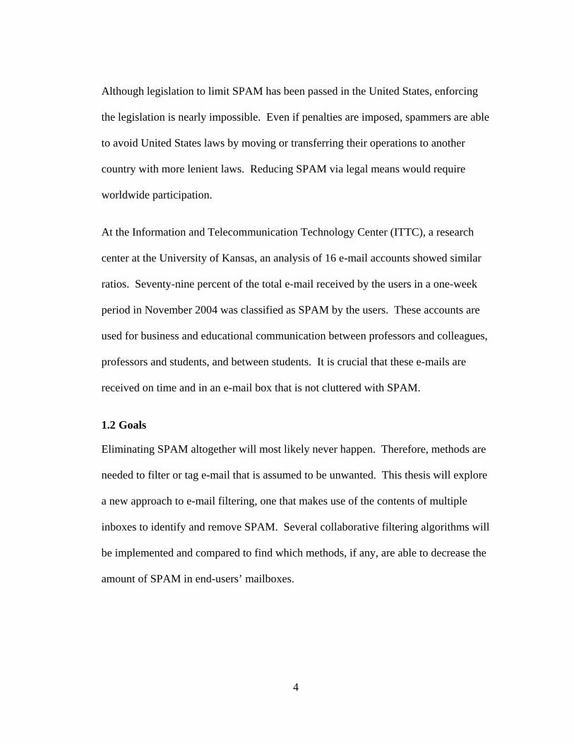
To understand the problem, first look at all of the locations where large quantities of
e-mail addresses can be seen, or harvested, by spammers. In November of 2002,
1
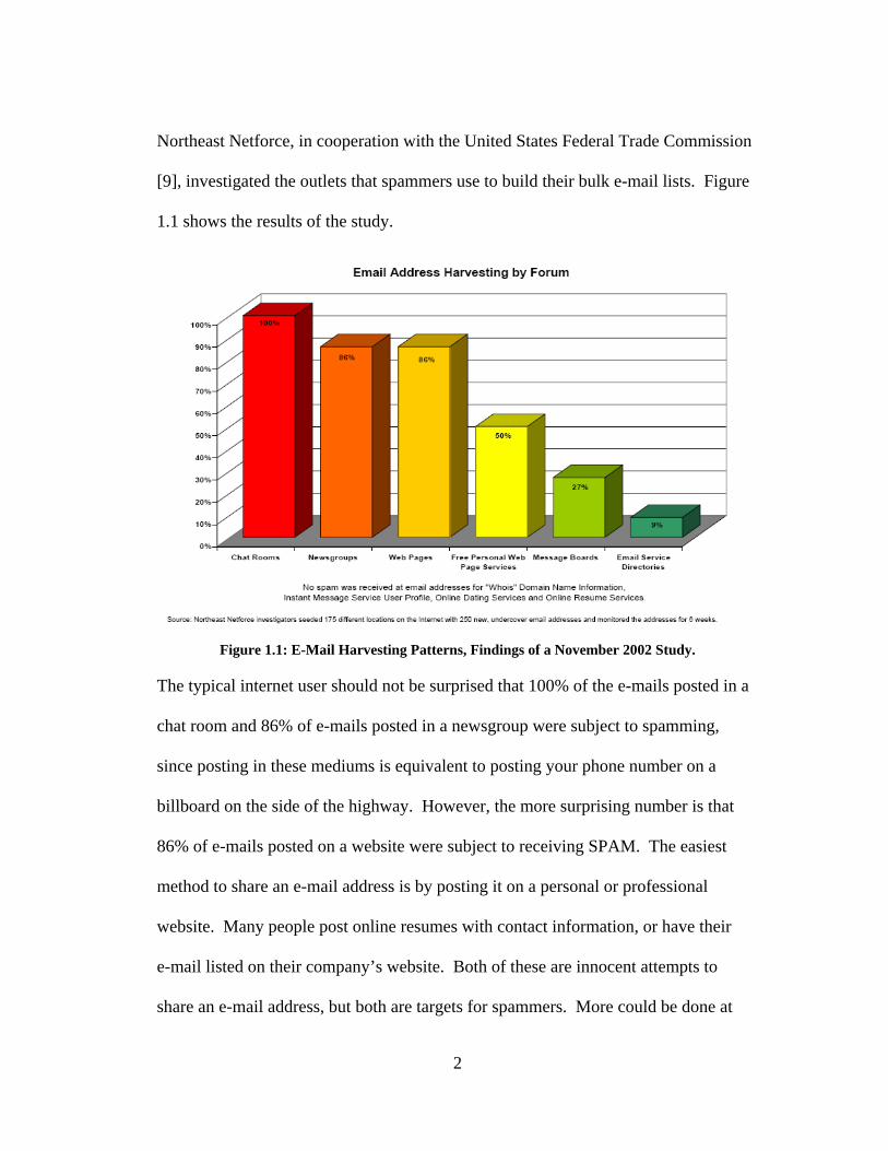
Northeast Netforce, in cooperation with the United States Federal Trade Commission
[9], investigated the outlets that spammers use to build their bulk e-mail lists. Figure
1.1 shows the results of the study.
Figure 1.1: E-Mail Harvesting Patterns, Findings of a November 2002 Study.
The typical internet user should not be surprised that 100% of the e-mails posted in a
chat room and 86% of e-mails posted in a newsgroup were subject to spamming,
since posting in these mediums is equivalent to posting your phone number on a
billboard on the side of the highway. However, the more surprising number is that
86% of e-mails posted on a website were subject to receiving SPAM. The easiest
method to share an e-mail address is by posting it on a personal or professional
website. Many people post online resumes with contact information, or have their
e-mail listed on their company’s website. Both of these are innocent attempts to
share an e-mail address, but both are targets for spammers. More could be done at
2
this level, such as disguising e-mail addresses through web scripts, or writing e-mail
addresses in plaintext, instead of the typical [email protected] format. These and
other methods are a step in the right direction to reduce the total amount of SPAM
received.
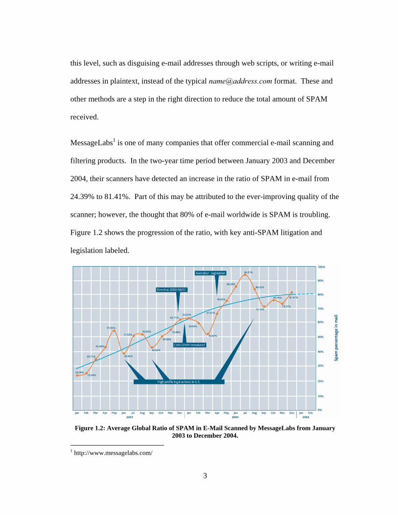
MessageLabs1 is one of many companies that offer commercial e-mail scanning and
filtering products. In the two-year time period between January 2003 and December
2004, their scanners have detected an increase in the ratio of SPAM in e-mail from
24.39% to 81.41%. Part of this may be attributed to the ever-improving quality of the
scanner; however, the thought that 80% of e-mail worldwide is SPAM is troubling.
Figure 1.2 shows the progression of the ratio, with key anti-SPAM litigation and
legislation labeled.
Figure 1.2: Average Global Ratio of SPAM in E-Mail Scanned by MessageLabs from January
2003 to December 2004. 1 http://www.messagelabs.com/
3
Although legislation to limit SPAM has been passed in the United States, enforcing
the legislation is nearly impossible. Even if penalties are imposed, spammers are able
to avoid United States laws by moving or transferring their operations to another
country with more lenient laws. Reducing SPAM via legal means would require
worldwide participation.
At the Information and Telecommunication Technology Center (ITTC), a research
center at the University of Kansas, an analysis of 16 e-mail accounts showed similar
ratios. Seventy-nine percent of the total e-mail received by the users in a one-week
period in November 2004 was classified as SPAM by the users. These accounts are
used for business and educational communication between professors and colleagues,
professors and students, and between students. It is crucial that these e-mails are
received on time and in an e-mail box that is not cluttered with SPAM.
1.2 Goals
Eliminating SPAM altogether will most likely never happen. Therefore, methods are
needed to filter or tag e-mail that is assumed to be unwanted. This thesis will explore
a new approach to e-mail filtering, one that makes use of the contents of multiple
inboxes to identify and remove SPAM. Several collaborative filtering algorithms will
be implemented and compared to find which methods, if any, are able to decrease the
amount of SPAM in end-users’ mailboxes.
4
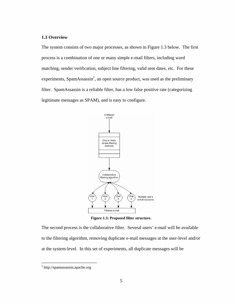
1.3 Overview
The system consists of two major processes, as shown in Figure 1.3 below. The first
process is a combination of one or many simple e-mail filters, including word
matching, sender verification, subject line filtering, valid sent dates, etc. For these
experiments, SpamAssassin2, an open source product, was used as the preliminary
filter. SpamAssassin is a reliable filter, has a low false positive rate (categorizing
legitimate messages as SPAM), and is easy to configure.
Figure 1.3: Proposed filter structure.
The second process is the collaborative filter. Several users’ e-mail will be available
to the filtering algorithm, removing duplicate e-mail messages at the user-level and/or
at the system-level. In this set of experiments, all duplicate messages will be
2 http://spamassassin.apache.org
5
removed at the user-level, and at the system-level, and the results will be compared.
Several variations of “duplicate” will be defined, using various parts of the e-mail
messages themselves.
The rest of this thesis is organized as follows: Chapter 2 discusses related work in the
area of SPAM filtering, including various algorithms and their performance. Chapter
3 gives a more detailed description of the process used to execute the algorithms.
Chapter 4 details the test data collection, along with the implementation of the
preliminary filter, SpamAssassin. Chapter 5 discusses the results of the applied
collaborative filter. Chapter 6 verifies the results found in the evaluation section, and
Chapter 7 summarizes the findings and draws conclusions.
6
Chapter 2: Related Work
2.1 SPAM Filter Basics
Researchers have been applying text categorization methods to the ever-changing
problem of SPAM for about ten years. The resulting filters can be applied at the
user-level, or at the system-level. At the user-level, e-mail programs, such as
Outlook, Eudora, and web-based e-mail readers allow users to create custom rules to
sort and filter mail. The rules they create only apply to their e-mail and do not apply
to other users that share the same e-mail service. Various software packages such as
Norton Anti-SPAM3 and McAfee SPAM Killer4 run on personal computers, and
provide a local filter for the end-user. The user-level filter can be configured
differently for each user, and the specific types of SPAM messages the user receives.
System-level filters tag or delete SPAM as the e-mail server receives the message.
Filters such as SpamAssassin5, can be run at the system-level or user-level, and can
be set up to insert a variable in the e-mail header, if a message is detected as SPAM
by the filter. The user can then configure their e-mail client to deal with the messages
how they choose. One advantage of the system-level filter is that it can track message
distribution statistics over a large group of users and detect bulk spammers and the
mail servers they use.
3 http://www.symantec.com/ 4 http://www.mcafee.com/ 5 http://spamassassin.apache.org/
7
2.2 Various Algorithms in SPAM Filtering
There have been, and continue to be, many attempts to filter e-mail using tested text
classification filtering methods. The following sections will attempt to summarize the
more popular algorithms.
2.2.1 Rule-Based Systems
The first and simplest SPAM filtering method is the rule-based system. A user
defines specific rules to deal with specific senders, subject lines, or words in a
message. Rules as simple as “if message subject includes ‘FREE’, then delete
message,” can detect a moderate amount of SPAM, and these approaches were
adequate just a couple years ago. With a large enough collection of specific rules, all
SPAM messages could be detected, and removed from a user’s mailbox. As SPAM
developed, spammers changed their tactics, and began camouflaging SPAM messages
to try to get around these concise rules. In order to keep up with the changing nature
of SPAM, a user would need to edit his/her rules daily, if not hourly. Eventually, it is
no longer efficient to hand-code all of these rules, and researchers realized the need
for more adaptable methods of filtering.
Applying automatic rule generating algorithms to e-mail filtering was the next logical
step. Cohen [5] developed RIPPER circa 1995 for text characterization. RIPPER
forms rules for a data set one by one until all desired cases are covered. Then, the
rules are minimized for a rule set. RIPPER was slightly modified to filter e-mail, as
described in a later paper by Cohen, and detailed in Section 2.2.2 of this document.
8
2.2.2 Statistical Information Retrieval (IR) Methods Versus Learning Rules
Rule-based approaches generally do not scale to the complexity and diversity present
in modern SPAM. Thus, most current approaches are based on statistical analysis of
message contents. The basic idea is to provide a measure of similarity between
messages. In a vector-space approach, each e-mail is represented as a vector of
words, where each word is given a score depending on the number of instances of the
word in the e-mail, the number of instances of the word in the corpus, and the length
in words of the e-mail. The score is typically calculated using some variation of the
term frequency – inverse document frequency (TF-IDF) formula. The given score
increases with the number of times the word appears in the e-mail (the term
frequency) but is offset by the number of times the word appears in the entire data set
(the inverse document frequency).
All of the vectors corresponding to legitimate e-mails are added and all vectors
corresponding to SPAM e-mails are subtracted, resulting in a “prototypical vector”.
A threshold is defined for the corpus, and if an e-mail’s vector is within that threshold
to the prototype, the e-mail receives a positive score.
Cohen [6] compares TF-IDF weighting to RIPPER [5], a rule-learning algorithm.
RIPPER, mentioned earlier, was modified in this case to take into account a loss ratio:
a penalty for misclassifying a legitimate message as SPAM. Cohen tokenizes the To,
From, Subject, and first 100 words of each message in the experiments. Among other
tests mentioned, TF-IDF and RIPPER were used to filter mail into 11 mailboxes over
9
three users. The percentage of data used for training was altered from 5% to 80%,
resulting in error rates from ~0.15 for TF-IDF and ~0.12 for RIPPER on 5% training,
to ~0.061 for TF-IDF and ~0.059 for RIPPER with 80% training.
He concluded that learning rules are competitive with traditional IR learning methods,
and a combination of user-constructed and machine learned rules are a viable filtering
system. Unfortunately, these results cannot be directly related to other methods
mentioned in this section, because Cohen did not use precision versus recall, or
accuracy in his analysis.
2.2.3 Naïve Bayesian Filters
Naïve Bayesian filtering has proven the most popular in current filtering attempts.
There are many variations of Naïve Bayes, but the basic principle is to calculate the
probability that an e-mail belongs to the class of legitimate e-mails or the class of
SPAM e-mails. This is done by calculating a score for each word in a training data
set: the probability that the word is likely to appear in a SPAM message and/or a
legitimate message. When a new message arrives, all of the words are queried for
their probabilities, the probabilities are summed based on existence or absence of the
word, and if the resulting score is higher than a pre-defined threshold, the message is
classified as SPAM. The thresholds are proportional to the penalty of misclassifying
a legitimate message as SPAM. For instance, if it is 999 times worse to misclassify a
legitimate message than to let a SPAM message get through the filter, then the
10
threshold t=0.999. If letting a SPAM message through the filter is the same as
misclassifying a legitimate message (1x), the threshold is t=0.5.
In 1998, Sahami et al. [14] are credited as the first to use a Naïve Bayesian classifier
to classify e-mail. The classifier was trained on manually categorized e-mail
messages. The subject and the body of each message were converted into a vector,
with each word having a mutual information score. All words that appeared less than
three times in the corpus were removed, and the top 500 words based on mutual
information score were used in the classification process. Three different
combinations of attributes were used in the experiments. The first was strictly words
with a resulting SPAM precision of 97.1% and recall of 94.3%. The second
algorithm combined words and manually chosen phrases. This algorithm yielded a
SPAM precision of 97.6% and recall of 94.3%. The third algorithm added non-
textual features of an e-mail, such as attachments, the sender’s domain, etc. This
algorithm had a 100% precision and 98.3% recall rate.
Those three experiments were performed on a data set where 88.2% of the messages
were SPAM. A fourth experiment was run with the highest algorithm, number three,
on a data set which was 20% SPAM, a more accurate approximation of SPAM in real
e-mail at the time, with a precision of 92.3% and recall of 80.0%. All experiments
were performed with a threshold of t=0.999.
11
Androutsopoulos et al. [1] followed shortly after, building a naïve Bayesian filter,
using the Ling-SPAM6 list as the data set. The collection is a mixture of 16.6%
SPAM messages and messages from the Linguist list, a moderated list “about the
profession and science of linguistics.” Although the legitimate messages in his data
set were not actual e-mails, he claims that because they contain postings from job
announcements, information about software, and some “flame-like” responses, it is
the closest thing to real e-mail available at that time.
Androutsopoulos et al. used only the text features of e-mail and added a lemmatizer, a
function to convert each word to its base form, and a stoplist, to remove the 100 most
frequent words of the British National Corpus (BNC). Several variations of
enabled/disabled lemmatizer and stoplist were tested with a variety of thresholds.
Because a large penalty should be given to miscategorizing legitimate messages, and
to accurately compare Androutsopoulos’s work to Sahami, the results from a
threshold of t=0.999 are the only results mentioned here. The best algorithm included
the lemmatizer but not the stopword features, and resulted in a precision of 100%
with a recall of 63.05%. The conclusion was that naïve Bayesian filtering is not
viable for such a high threshold.
The Naïve Bayesian algorithm is simple to implement and scales well to large-scale
training data [11], providing an efficient filtering mechanism.
6 http://www.mlnet.org/
12
2.2.4 Memory-Based Filtering
Androutsopoulos [2] again compares the Naïve Bayesian Filter of Sahami et al. [14],
but this time to a memory-based classifier named TiMBL [8]. Ling-SPAM is again
used as the corpus, with 16.6% of the messages being SPAM. Vectors are computed
for each message, where each item in the vector corresponds to the existence or
absence of a particular attribute. A ‘1’ is stored in the corresponding vector location
if the attribute is found in the message, and a ‘0’ if the attribute is absent in the
message. The mutual information (MI) was figured for each attribute and the top m
attributes, based on MI were retained. The number of retained attributes was varied
in the experiments from 50 to 700. As in [1], a lemmatizer was applied to the Ling-
SPAM collection to improve attribute accuracy.
The memory-based method stores all training data in a memory structure to used for
classification of incoming messages. The algorithm considers the k most closely
related vectors to the one in question in order to make a judgment. The k needs to be
as small as possible to avoid considering vectors that are very different from the one
in question. In this experiment k=1, 2, and 10 were each used. Again, multiple
thresholds were used in the experiments, although only the results for t=0.999 (which
weights misclassifying one legitimate message as SPAM equal to letting 999 SPAM
messages through the filter) will be discussed here, to accurately compare the
memory-based algorithm to previously discussed algorithms.
13
TiMBL with k=1 was outperformed by Naïve Bayes across the board. TiMBL with
k=2 and k=10 outperformed Naïve Bayes except when the number of retained
attributes was 300. The best configuration of Naïve Bayes yielded precision of 100%
with recall of 63.67 when 300 attributes were used. The optimal TiMBL setup was
k=2, with 250 attributes. The resulting precision was 100% with 54.30% recall. In
the memory-based approach’s defense, it did outperform the Naïve Bayesian filter
when the threshold was t=0.5 (where tagging a legitimate message as SPAM is equal
to letting 1 SPAM message through the filter).
2.2.5 Collaborative Filtering
All of the above methods are content-based filters, where classification is based on
the content of the e-mail in question. Another method of classifier gaining attention
is the collaborative approach. Many collaborative filters [3][4][13] have been applied
as recommender systems to recommend movies, television programs, or interesting
websites.
Collaborative filters used as recommender systems attempt to classify unseen items of
a user into one of two classes: like or dislike. This is done by finding a user or users
that have judged the unseen item, and using the judgment of the most similar user
based on past judgments. Sometimes the judgment is made indirectly. For instance,
if users A and B are closely related, and so are B and C, then it might be assumed that
users A and C are related. This is key if user A is looking for a judgment, but user B
has not rated the item in question and user C has. Billsus and Pazzani [3] also take
14
into account negatively correlated users. User A’s positive ratings might predict a
negative rating for user B, if the users are negatively correlated.
Breese et al. [4] detail a collaborative recommender system that queries multiple
users based on their degree of similarity to the user trying to make a decision. A
small number of user recommendations increases the likelihood that a correct
prediction will be made. There is a point where a high number of recommendations
become a negative feature, mostly because each additional recommender is less
similar to the user in question than the previous recommender.
There have been few applications of collaborative filtering applied to SPAM
filtering. Cunningham et al. [7] notes, “Collaborative approaches do not care about
the content of the email, but on the users who share information about SPAM.” If a
person receives a SPAM message, he/she can share a signature for the message so
that later receivers can be on the lookout for the same SPAM message. The signature
generation method has to be robust in order to account for small changes in the body
and subject of the message, such as the insertion of random text, or letter substitution.
Vipul’s Razor [18] is an early application of a collaborative approach, using a central
catalogue for sharing signatures. Razor’s accuracy is reported at 60% – 90%, which
is attributed to the fact that it is used by a wide variety of people, instead of just one
company, Internet service provider (ISP), or person.
Performance data on a collaborative e-mail filter could not be located to be included
as a comparison to content-based filtering.
15
2.2.6 Blacklists and Whitelists
Another filtering mechanism that does not particularly look at the content of the
message is origin-based filters; the two most popular being blacklists and whitelists.
There are two methods of blacklisting; the first is blocking Internet Protocol (IP) or
Transmission Control Protocol (TCP) connections from known open relay servers or
from known spammers, or by blocking based on the domain name of the sender. The
latter is not as effective because of servers that can be used as open relays. There are
multiple online databases of known relays and domains used by spammers [12] [16].
The second method is by using reverse lookup of the sender’s IP address based on the
sender’s domain name, and comparing that to the actual originating IP address of the
message.
Whitelists are lists of trusted senders, set up by the e-mail recipient. Only messages
sent from trusted senders are allowed into the mailbox, and all other messages will be
returned to the sender. The standard is that if the sender replies to the rejected
message within a certain amount of time, they will be assumed to be a legitimate
sender, and they will be added to the whitelist, and their messages will go through the
filter from that point forward. The end-user, however, should have ultimate control
and be able to override any sender on the whitelist. This “bouncing” of messages
back and forth can get tiring and frustrating for most e-mailers that are looking for a
quick means of communication.
16
Chapter 3: Approach
Since spammers send basically the same message to hundreds of thousands of people
at a time, it should be possible to locate similar messages in a large set of messages,
and be able to draw some conclusions about the messages. The filter discussed here
will attempt to remove some of the SPAM received by the Information and
Telecommunication Center (ITTC) users using this idea.
Sixteen people volunteered their e-mail for the testing and validation experiments.
Because of quantity and type of e-mails received per user, only nine people’s e-mail
could be used in the experiments. The test collection and selection of users is
discussed in Chapter 4. After the e-mail was collected and a baseline was established,
all of the messages were loaded into a database for analysis. Using several different
algorithms, the messages were compared to each other to find duplicates. All
duplicate messages were deleted; how many legitimate and how many SPAM
messages were deleted each time was documented. For each algorithm, first
messages with two or more copies were deleted, then messages with three or more
copies, then four, and so on. The resulting accuracy, recall, precision, and F-measure
were calculated, and form the basis of comparison of the algorithms. The discussion
of those results are in Chapter 5.
17
Chapter 4: Test Collection
4.1 Overview
Sixteen volunteers with e-mail accounts at ITTC chose to volunteer their incoming
e-mail for a period of two weeks. The e-mail from week one was used as the testing
data set, and week two as the validation data set. The sixteen volunteers consisted of
two professors, three Ph.D. students, seven graduate students, two undergraduate
students, and two staff members. A wide variety of roles at ITTC was needed to
ensure a varied e-mail collection.
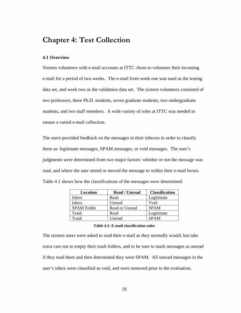
The users provided feedback on the messages in their inboxes in order to classify
them as: legitimate messages, SPAM messages, or void messages. The user’s
judgments were determined from two major factors: whether or not the message was
read, and where the user stored or moved the message to within their e-mail boxes.
Table 4.1 shows how the classifications of the messages were determined:
Location Read / Unread Classification Inbox Read Legitimate Inbox Unread Void SPAM Folder Read or Unread SPAM Trash Read Legitimate Trash Unread SPAM
Table 4.1: E-mail classification rules
The sixteen users were asked to read their e-mail as they normally would, but take
extra care not to empty their trash folders, and to be sure to mark messages as unread
if they read them and then determined they were SPAM. All unread messages in the
user’s inbox were classified as void, and were removed prior to the evaluation.
18
4.2 Collection Statistics
Table 4-2 details the breakdown of message classifications per user and for the set as
a whole.
User Total
Messages LegitimateMessages % SPAM %
Spam-Assassin %
Void Messages
1 818 70 9% 747 91% 675 90% 1 2 17 7 41% 1 6% 0 0% 9 3 51 45 88% 6 12% 0 0% 0 4 922 236 26% 676 73% 641 95% 10 5 434 105 24% 324 75% 292 90% 5 6 11 11 100% 0 0% 0 0% 0 7 8 0 0% 7 88% 0 0% 1 8 8 7 88% 0 0% 0 0% 1 9 54 12 22% 19 35% 16 84% 23 10 305 32 10% 252 83% 194 77% 21 11 3 3 100% 0 0% 0 0% 0 12 8 2 25% 0 0% 0 0% 6 13 106 5 5% 89 84% 8 9% 12 14 1516 228 15% 1286 85% 1088 85% 2 15 0 0 0% 0 0% 0 0% 0 16 48 43 90% 1 2% 0 0% 4
Totals 4309 806 19% 3408 79% 2914 86% 95
Table 4.2: E-mail statistics per user, and for the entire set of users
The table shows a wide variety in the amount of e-mail across the users. The
maximum e-mails received for one user was 1,516, which is more than 1/3 of the total
e-mails received for the entire group. The percentage of legitimate e-mails received
per user varies from 0% to 100%, with the average per user at 19%.
4.3 User Selection
From Table 4.2 above, it is obvious that some users did not receive enough e-mail, or
enough SPAM, to be good candidates for evaluating information and value to the test
data set than others. User 15 is removed from the data set, because he/she had no
19
e-mail in his/her inbox at the end of week 1. Users 6 and 11 did not receive any
SPAM messages during the time period and received very few messages; 11 and 3
respectively7. User 7 did not receive any legitimate messages, with only 8 messages
total. Users 2, 8, and 12 were excluded because of the low number of messages
received in the time period: 17, 8, and 8 messages respectively. These factors may
have been a human error where the user emptied his/her trash folder during week 1,
or the user may not use his/her ITTC e-mail account as a primary e-mail address.
After excluding these users from further study, nine users remained.
4.4 Determination of Baseline
After the users were selected based on their e-mail usage statistics, the messages were
ready to enter the preliminary filtering stage of the process. Void messages were
removed, e-mail sent within the system was removed, and SpamAssassin was applied
to the messages, resulting in the data set that was used for the evaluation of
collaborative filtering algorithms.
4.4.1 Void Message Removal
All messages with void classification were removed from the data set. These were
messages that were located in the users’ inboxes, but were unread. It is implied that
these are messages that were received by the mail server, and not yet classified by the
user. Ninety-five messages, or 2% of the original data set were classified as void and
removed. Seventy-eight messages were removed from the data set.
7 User 16 remains in the data set because he/she received 43 messages in the time period, a relatively high number of legitimate messages for the one-week time period.
20
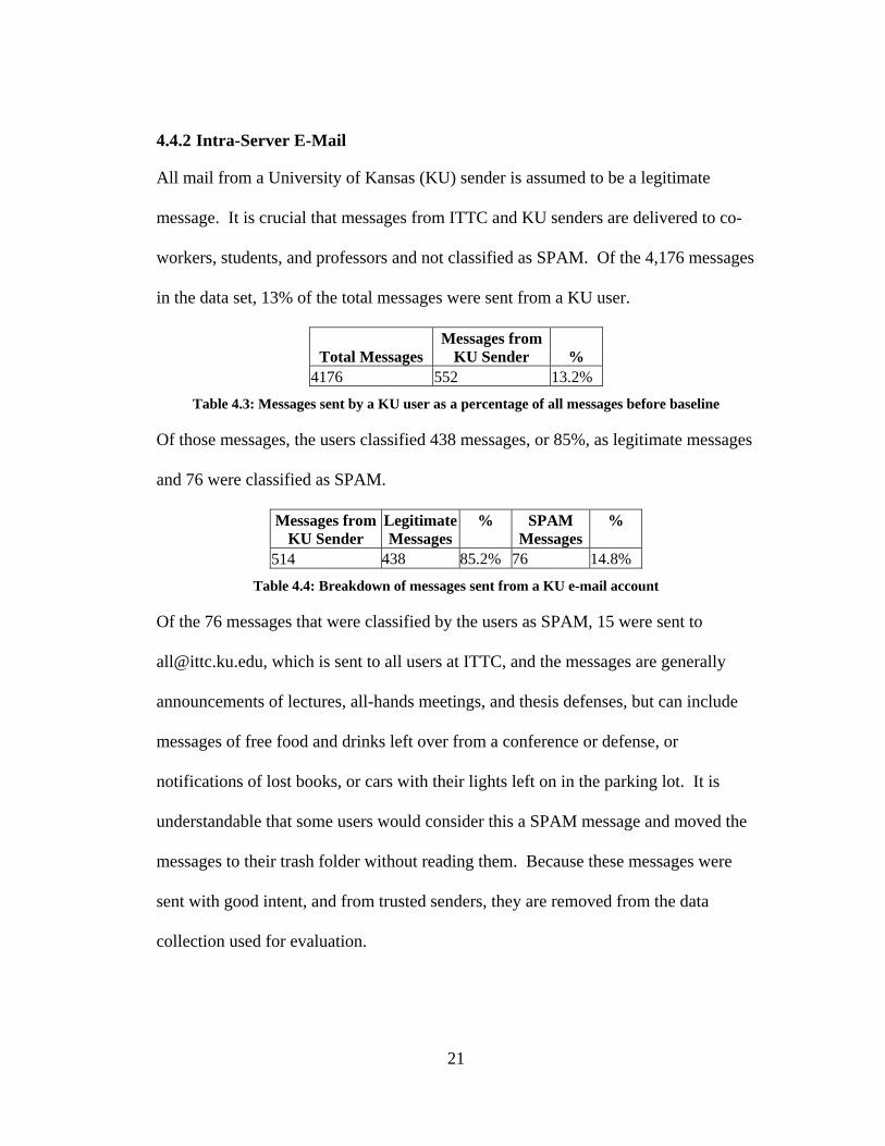
4.4.2 Intra-Server E-Mail
All mail from a University of Kansas (KU) sender is assumed to be a legitimate
message. It is crucial that messages from ITTC and KU senders are delivered to co-
workers, students, and professors and not classified as SPAM. Of the 4,176 messages
in the data set, 13% of the total messages were sent from a KU user.
Total Messages Messages from
KU Sender % 4176 552 13.2%
Table 4.3: Messages sent by a KU user as a percentage of all messages before baseline
Of those messages, the users classified 438 messages, or 85%, as legitimate messages
and 76 were classified as SPAM.
Messages fromKU Sender
LegitimateMessages
% SPAM Messages
%
514 438 85.2% 76 14.8%
Table 4.4: Breakdown of messages sent from a KU e-mail account
Of the 76 messages that were classified by the users as SPAM, 15 were sent to
[email protected], which is sent to all users at ITTC, and the messages are generally
announcements of lectures, all-hands meetings, and thesis defenses, but can include
messages of free food and drinks left over from a conference or defense, or
notifications of lost books, or cars with their lights left on in the parking lot. It is
understandable that some users would consider this a SPAM message and moved the
messages to their trash folder without reading them. Because these messages were
sent with good intent, and from trusted senders, they are removed from the data
collection used for evaluation.
21
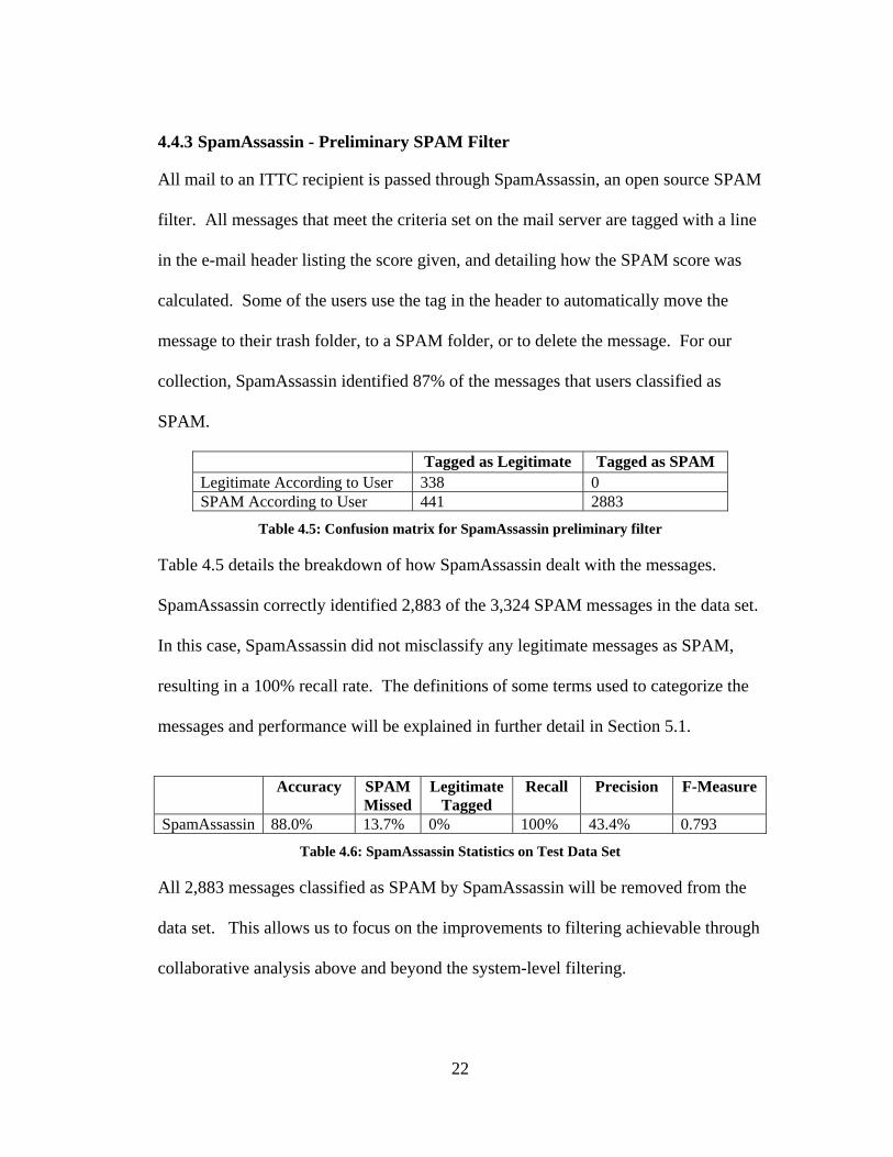
4.4.3 SpamAssassin - Preliminary SPAM Filter
All mail to an ITTC recipient is passed through SpamAssassin, an open source SPAM
filter. All messages that meet the criteria set on the mail server are tagged with a line
in the e-mail header listing the score given, and detailing how the SPAM score was
calculated. Some of the users use the tag in the header to automatically move the
message to their trash folder, to a SPAM folder, or to delete the message. For our
collection, SpamAssassin identified 87% of the messages that users classified as
SPAM.
Tagged as Legitimate Tagged as SPAM Legitimate According to User 338 0 SPAM According to User 441 2883
Table 4.5: Confusion matrix for SpamAssassin preliminary filter
Table 4.5 details the breakdown of how SpamAssassin dealt with the messages.
SpamAssassin correctly identified 2,883 of the 3,324 SPAM messages in the data set.
In this case, SpamAssassin did not misclassify any legitimate messages as SPAM,
resulting in a 100% recall rate. The definitions of some terms used to categorize the
messages and performance will be explained in further detail in Section 5.1.
Accuracy SPAM
Missed Legitimate
Tagged Recall Precision F-Measure
SpamAssassin 88.0% 13.7% 0% 100% 43.4% 0.793
Table 4.6: SpamAssassin Statistics on Test Data Set
All 2,883 messages classified as SPAM by SpamAssassin will be removed from the
data set. This allows us to focus on the improvements to filtering achievable through
collaborative analysis above and beyond the system-level filtering.
22
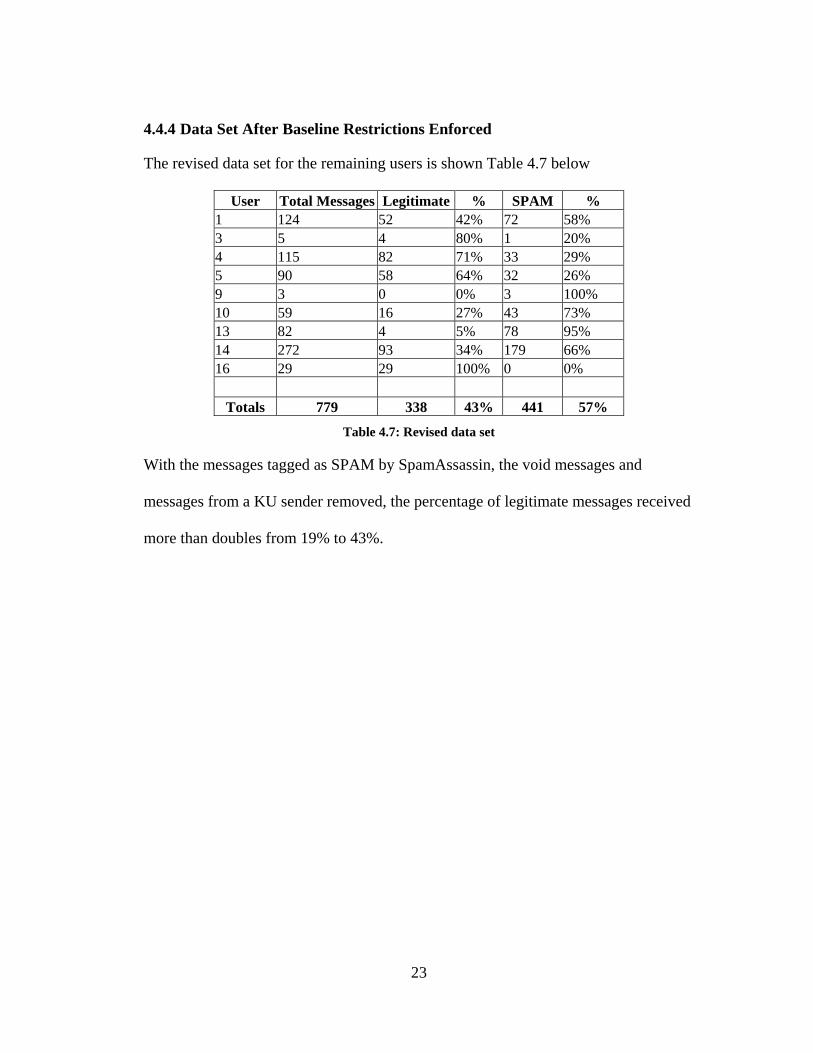
4.4.4 Data Set After Baseline Restrictions Enforced
The revised data set for the remaining users is shown Table 4.7 below
User Total Messages Legitimate % SPAM % 1 124 52 42% 72 58% 3 5 4 80% 1 20% 4 115 82 71% 33 29% 5 90 58 64% 32 26% 9 3 0 0% 3 100% 10 59 16 27% 43 73% 13 82 4 5% 78 95% 14 272 93 34% 179 66% 16 29 29 100% 0 0%
Totals 779 338 43% 441 57%
Table 4.7: Revised data set
With the messages tagged as SPAM by SpamAssassin, the void messages and
messages from a KU sender removed, the percentage of legitimate messages received
more than doubles from 19% to 43%.
23
Chapter 5: Evaluation
5.1 Evaluation Criteria
For each algorithm, the results were calculated and placed in a confusion matrix as
shown in Table 5.1. Messages in the “legitimate removed” box are most commonly
referred to as false positives, because they are legitimate messages classified as
SPAM. Messages in the “SPAM passed” box are most commonly referred to as false
negatives, because they are SPAM messages that have been overlooked by the filter.
Tagged as Legitimate
Tagged as SPAM
Legitimate According to User Legitimate Passed
Legitimate Removed
SPAM According to User SPAM Passed SPAM Removed
Table 5.1: Confusion matrix for classifying messages.
The accuracies, recall, and precision of each algorithm are calculated by equations
one through three below. These calculations are completed for each quantity of
messages removed in the algorithms (i.e. two or more copies removed, three or more,
etc.).
Set Data in the Messages AllRemoved SPAMPassed LegitimateAccuracy +
=
Equation 5.1: Accuracy of Algorithm
Removed LegitimatePassed LegitimatePassed LegitimateRecall
+=
Equation 5.2: Recall of Algorithm
Passed SPAMPassed LegitimatePassed LegitimatePrecision+
=
Equation 5.3: Precision of Algorithm
24
Using the precision and recall calculations, the F-measure of each algorithm was
calculated:
RecallPrecisionRecallPrecision)1(F 2
2
+×××+
=ββ
Measure
Equation 5.4: F-Measure of Algorithm
where β is a constant with a value from 0 to infinity. We chose to use β=2.0 because
this places a higher emphasis on recall, receiving legitimate messages, over precision,
eliminating SPAM. This is important because for all of the algorithms, a 100%
precision cannot be achieved. This is because the algorithms only deal with duplicate
messages, and do not attempt to classify unique messages. This forms an upper
bound on the precision, which on average is 0.50. This upper bound also affects the
F-measures, resulting in an average upper bound on F-measures of 0.825. The
highest F-measures point for each algorithm is used in the comparison between the
algorithms.
5.2 Number of Recipients and Number of Received Messages
The main idea of collaborative filtering in an e-mail system is to be able to apply
actions of a single user to the entire set of users. For example, if more than one user
receives the same message, what can the system do to ensure all users do not have to
deal with the same message.
For collaborative filtering to be effective, several instances of a message must appear
in the data set. Table 5.2 shows the breakdown of the percent of unique legitimate
25
and SPAM messages for the revised data set. The number of unique SPAM messages
in the entire set is 67%, and for some users as low as 0%.
User Total
Messages Legitimate
Unique Legitimate on subject % SPAM
Unique SPAM on subject %
1 124 52 26 50% 72 28 39% 3 5 4 4 100% 1 1 100% 4 115 82 50 61% 33 27 82% 5 90 58 47 81% 32 3 9% 9 3 0 0 0% 3 1 33% 10 59 16 10 63% 43 41 95% 13 82 4 4 100% 78 57 73% 14 272 93 57 61% 179 137 77% 16 29 29 17 44% 0 0 0% Totals 779 338 215 64% 441 295 67%
Table 5.2: Number of unique messages, legitimate and SPAM
A graphical representation of the distribution statistics is shown in Figure 5.1. The
majority of the e-mail messages in the data set are unique, although one-third of all
remaining SPAM messages appear more than once in the data set.
26
215
123
295
146
0
50
100
150
200
250
300
350
400
450
Distribution Statistics of Messages
Duplicate Messages 123 146
Unique Messages 215 295
Legitimate SPAM
Figure 5.1: Distribution statistics of legitimate and SPAM messages
In the algorithms, three different characteristics of an e-mail message are used to
define which of the messages are duplicates. A duplicate message is defined in this
set of experiments as a copy based on a variety of comparison criteria. In the first
two algorithms, the subject lines of the messages are compared, in the next two
algorithms, the bodies of the messages are used, and in the last two algorithms, the
senders of the messages are compared.
For each definition of “duplicate” there are two types of duplicates: those within a
user’s inbox (i.e., user-level duplicates), and those that appear in different user’s
inboxes (i.e., system-level duplicates). For the user-level duplicates, if two messages
exist in one user’s mailbox with the same subject, the messages count as one message
27
with two copies. If three messages have the same subject, they count as one message
with three copies.
At the system-level, if two messages in the data set, independent of recipient, have
the exact same subject, they count as one message with two copies.
Depending on the algorithm’s definition of duplicate, the same data set may be seen
as containing anywhere from one to twelve duplicates for a given message. This
makes it difficult to compare algorithms, and increases the need for a universal
measure, such as the F-measure.
The evaluation of each algorithm includes a bar graph of the distribution statistics of
the messages. After the number of copies of each message is found, the messages are
grouped according to their classification by the user. If a message had two copies,
and the user classified both as SPAM, that message counted as one message with two
copies in the SPAM column. However, for a message with two copies, if a user
classified one of the copies as SPAM and the other as legitimate, the message counted
as one message with two copies, one in each of the SPAM and legitimate columns of
the distribution graph.
5.3 Duplicate Messages, Based on Subject
The first of the three qualities of the message used for defining duplicates is the
subject line of the message.
28
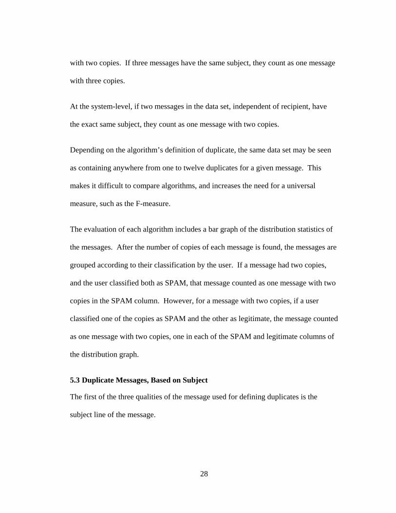
5.3.1 User-Level (Subject)
The user-level (subject) algorithm removed duplicate messages within each user’s
mailbox. In the data set, there were 634 messages that were unique to the users, and
60 different messages that appeared at least twice in the user’s mailboxes.
0
50
100
150
200
250
300
350
400
Instances
Copies
All Messages not sent from *ku.edu (or *ukans.edu) after Baseline
Legitimate Messages 258 19 8 2 2 0 1
SPAM Messages 376 21 3 2 0 2 0
1 2 3 4 5 6 7
Figure 5.2: Distribution statistics of messages based on duplication of subject within each user's
mailbox
Figure 5.2 shows the distribution statistics of the messages in the data set. One user
received a message with the same subject seven times in the one-week data collection
period. In this instance, the user categorized the message with seven copies as a
legitimate message. The most copies of a SPAM message was six copies, received
either by two different users, or a single user received two messages six times each.
29

0
5
10
15
20
25
Instances
Copies
All Messages not sent from *ku.edu (or *ukans.edu) after Baseline
Legitimate Messages 19 8 2 2 0 1
SPAM Messages 21 3 2 0 2 0
2 3 4 5 6 7
Figure 5.3: Distribution statistics of messages which occurred more than one time, based on
duplication of subject within each user's mailbox
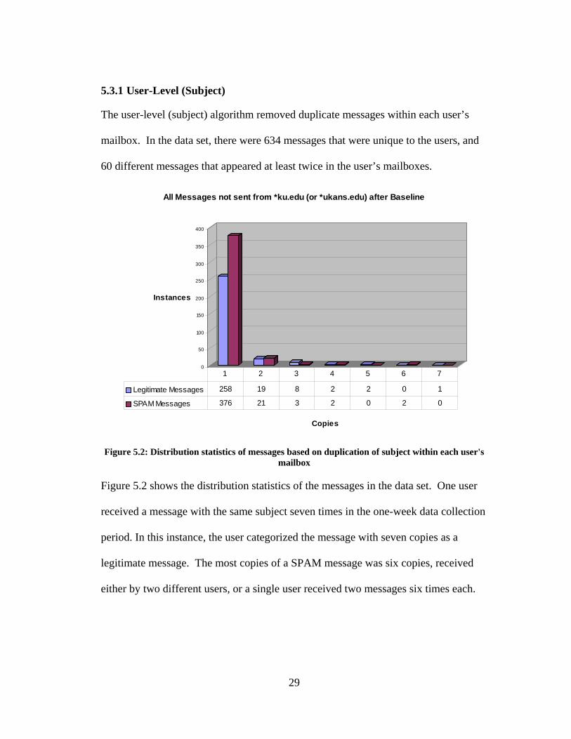
Figure 5.3 shows the distribution of messages with the exclusion of the unique
messages in the data set. The recall, precision, and resulting F-measure are shown in
Figure 5.4. The upper bound for these calculations was 0.473 for precision and 0.818
for F-measure.
30
Precision, Recall and F-Measure
0.00
0.20
0.40
0.60
0.80
1.00
1.20
Copies
Recall 0.763 0.867 0.932 0.950 0.979 0.979
Precision 0.407 0.414 0.427 0.428 0.436 0.429
F-Measure 0.650 0.711 0.754 0.764 0.782 0.779
2 3 4 5 6 7
Figure 5.4: Recall, precision and F-measure of the user-level (subject)
When messages with six or more copies are removed from the data set, the resulting
precision is the greatest, at 0.782 (96% of the upper bound F-measure of 0.818), with
12 SPAM messages being removed and seven legitimate messages being removed.
When seven messages are removed, the precision decreases, resulting in a lower
F-measure.
31

Accuracy
0.00
0.10
0.20
0.30
0.40
0.50
0.60
0.70
0.80
0.90
1.00
Copies
Inst
ance
s
Accuracy 0.415 0.409 0.427 0.427 0.440 0.425
2 3 4 5 6 7
Figure 5.5: Accuracy of the user-level (subject)
The accuracy of the algorithm is shown in Figure 5.5. The accuracy was highest
when six or more copies of messages were removed at a value of 0.440, which is 85%
of the upper bound of 0.517.
5.3.2 System-Level (Subject)
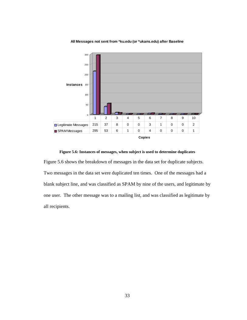
As in the first algorithm, the subject line of the e-mail messages in the data set was
used as the quantifier to determine duplicate messages. For this algorithm, messages
in the entire system were used to check for duplicates, instead of just comparing
messages within each mailbox, as in the user-level (subject) algorithm.
32
0
50
100
150
200
250
300
Instances
Copies
All Messages not sent from *ku.edu (or *ukans.edu) after Baseline
Legitimate Messages 215 37 8 0 0 3 1 0 0 2
SPAM Messages 295 53 6 1 0 4 0 0 0 1
1 2 3 4 5 6 7 8 9 10
Figure 5.6: Instances of messages, when subject is used to determine duplicates
Figure 5.6 shows the breakdown of messages in the data set for duplicate subjects.
Two messages in the data set were duplicated ten times. One of the messages had a
blank subject line, and was classified as SPAM by nine of the users, and legitimate by
one user. The other message was to a mailing list, and was classified as legitimate by
all recipients.
33
0
10
20
30
40
50
60
Instances
Copies
All Messages not sent from *ku.edu (or *ukans.edu) after Baseline
Valid Messages 37 8 0 0 3 1 0 0 2
Legitimate Messages 53 6 1 0 4 0 0 0 1
2 3 4 5 6 7 8 9 10
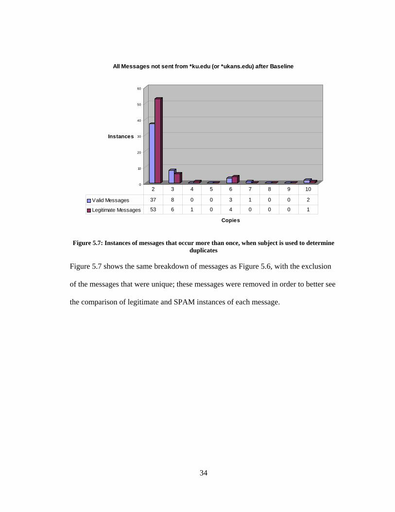
Figure 5.7: Instances of messages that occur more than once, when subject is used to determine
duplicates
Figure 5.7 shows the same breakdown of messages as Figure 5.6, with the exclusion
of the messages that were unique; these messages were removed in order to better see
the comparison of legitimate and SPAM instances of each message.
34
Precision, Recall and F-Measure
0.00
0.20
0.40
0.60
0.80
1.00
1.20
C o p ies
Recall 0.636 0.834 0.899 0.899 0.899 0.947 0.967 0.967 0.967
Precision 0.422 0.417 0.427 0.425 0.425 0.426 0.431 0.431 0.431
F-M easure 0.577 0.695 0.736 0.735 0.735 0.760 0.775 0.775 0.775
2 3 4 5 6 7 8 9 10
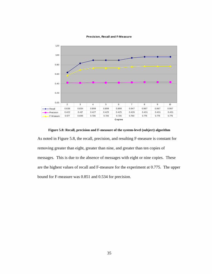
Figure 5.8: Recall, precision and F-measure of the system-level (subject) algorithm
As noted in Figure 5.8, the recall, precision, and resulting F-measure is constant for
removing greater than eight, greater than nine, and greater than ten copies of
messages. This is due to the absence of messages with eight or nine copies. These
are the highest values of recall and F-measure for the experiment at 0.775. The upper
bound for F-measure was 0.851 and 0.534 for precision.
35

Accuracy
0.00
0.10
0.20
0.30
0.40
0.50
0.60
0.70
0.80
0.90
1.00
C o p ies
Inst
ance
s
Accuracy 0.463 0.422 0.433 0.427 0.427 0.422 0.431 0.431 0.431
2 3 4 5 6 7 8 9 10
Figure 5.9: Accuracy of the system-level (subject) algorithm
The accuracy of the algorithm varied from the high point of 0.463 (75% of the upper
bound of 0.621) when two or more copies were removed, to the low point when seven
or more copies were removed.
5.4 Duplicate Messages, Based on Sender
The second of the three qualities of the message used for defining duplicates is the
sender of the message.
5.4.1 User-Level Sender Duplicates
The user-level (sender) algorithm removed duplicate messages within each users’
mailbox. In the data set, there were 457 messages that were unique to the users, and
117 different messages that appeared at least twice in the user’s mailboxes.
36
0
50
100
150
200
250
300
350
Instances
Copies
All Messages not sent from *ku.edu (or *ukans.edu) after Baseline
Legitimate Messages 135 38 28 5 5 0 1 1
SPAM Messages 322 37 7 2 3 2 1 1
1 2 3 4 5 6 7 8
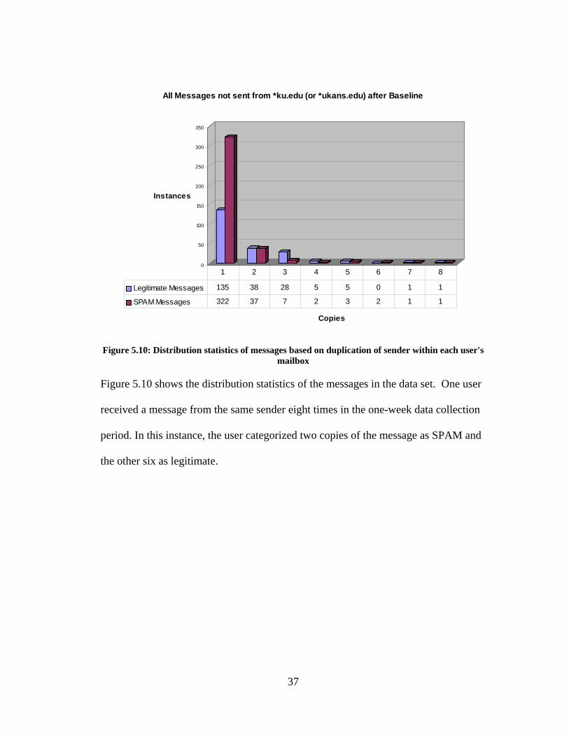
Figure 5.10: Distribution statistics of messages based on duplication of sender within each user's
mailbox
Figure 5.10 shows the distribution statistics of the messages in the data set. One user
received a message from the same sender eight times in the one-week data collection
period. In this instance, the user categorized two copies of the message as SPAM and
the other six as legitimate.
37
0
5
10
15
20
25
30
35
40
Instances
Copies
All Messages not sent from *ku.edu (or *ukans.edu) after Baseline
Legitimate Messages 38 28 5 5 0 1 1
SPAM Messages 37 7 2 3 2 1 1
2 3 4 5 6 7 8
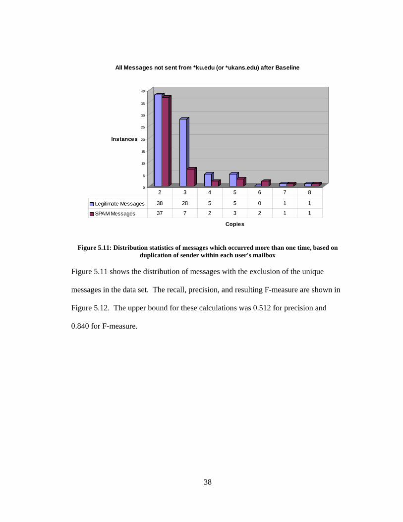
Figure 5.11: Distribution statistics of messages which occurred more than one time, based on
duplication of sender within each user's mailbox
Figure 5.11 shows the distribution of messages with the exclusion of the unique
messages in the data set. The recall, precision, and resulting F-measure are shown in
Figure 5.12. The upper bound for these calculations was 0.512 for precision and
0.840 for F-measure.
38
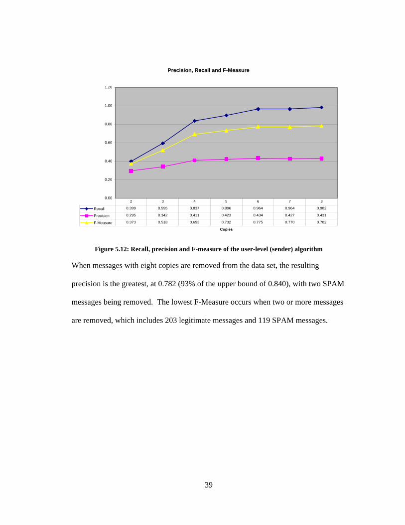
Precision, Recall and F-Measure
0.00
0.20
0.40
0.60
0.80
1.00
1.20
Copies
Recall 0.399 0.595 0.837 0.896 0.964 0.964 0.982
Precision 0.295 0.342 0.411 0.423 0.434 0.427 0.431
F-Measure 0.373 0.518 0.693 0.732 0.775 0.770 0.782
2 3 4 5 6 7 8
Figure 5.12: Recall, precision and F-measure of the user-level (sender) algorithm
When messages with eight copies are removed from the data set, the resulting
precision is the greatest, at 0.782 (93% of the upper bound of 0.840), with two SPAM
messages being removed. The lowest F-Measure occurs when two or more messages
are removed, which includes 203 legitimate messages and 119 SPAM messages.
39
Accuracy
0.00
0.10
0.20
0.30
0.40
0.50
0.60
0.70
0.80
0.90
1.00
Copies
Inst
ance
s
Accuracy 0.326 0.329 0.408 0.424 0.438 0.422 0.429
2 3 4 5 6 7 8
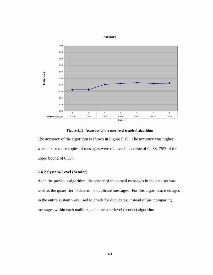
Figure 5.13: Accuracy of the user-level (sender) algorithm
The accuracy of the algorithm is shown in Figure 5.13. The accuracy was highest
when six or more copies of messages were removed at a value of 0.438, 75% of the
upper bound of 0.587.
5.4.2 System-Level (Sender)
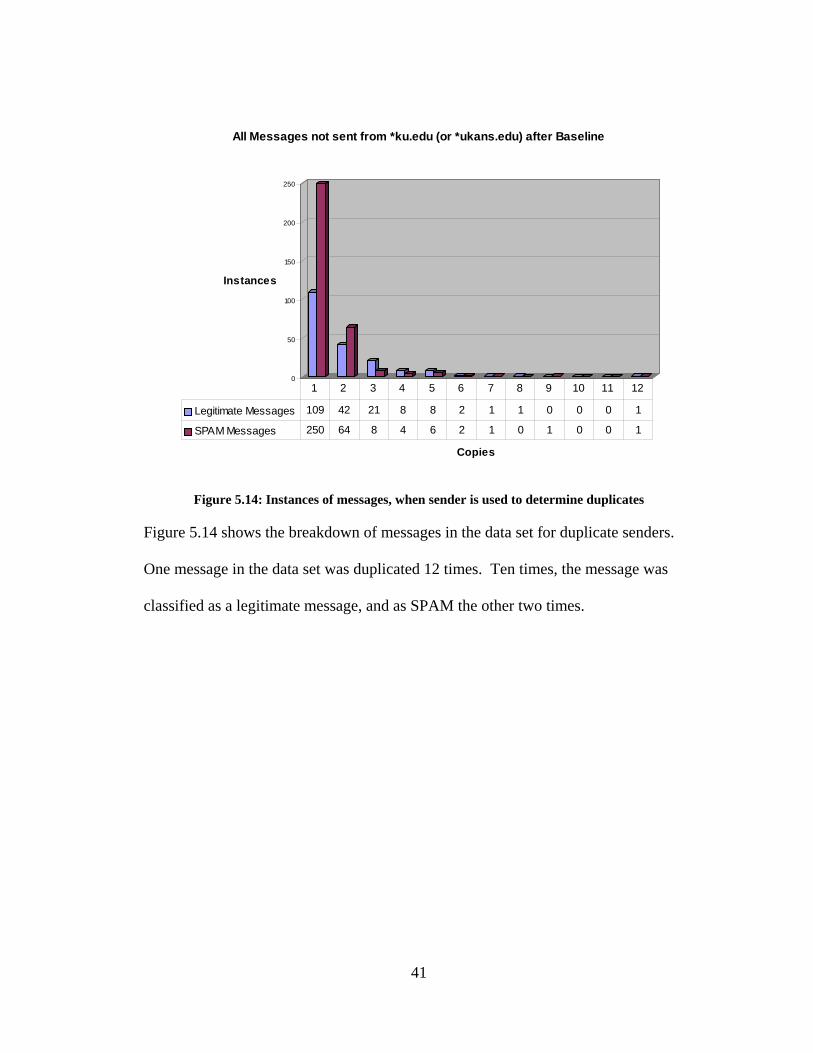
As in the previous algorithm, the sender of the e-mail messages in the data set was
used as the quantifier to determine duplicate messages. For this algorithm, messages
in the entire system were used to check for duplicates, instead of just comparing
messages within each mailbox, as in the user-level (sender) algorithm.
40
0
50
100
150
200
250
Instances
Copies
All Messages not sent from *ku.edu (or *ukans.edu) after Baseline
Legitimate Messages 109 42 21 8 8 2 1 1 0 0 0 1
SPAM Messages 250 64 8 4 6 2 1 0 1 0 0 1
1 2 3 4 5 6 7 8 9 10 11 12
Figure 5.14: Instances of messages, when sender is used to determine duplicates
Figure 5.14 shows the breakdown of messages in the data set for duplicate senders.
One message in the data set was duplicated 12 times. Ten times, the message was
classified as a legitimate message, and as SPAM the other two times.
41
0
10
20
30
40
50
60
70
Instances
Copies
All Messages not sent from *ku.edu (or *ukans.edu) after Baseline
Legitimate Messages 42 21 8 8 2 1 1 0 0 0 1
SPAM Messages 64 8 4 6 2 1 0 1 0 0 1
2 3 4 5 6 7 8 9 10 11 12
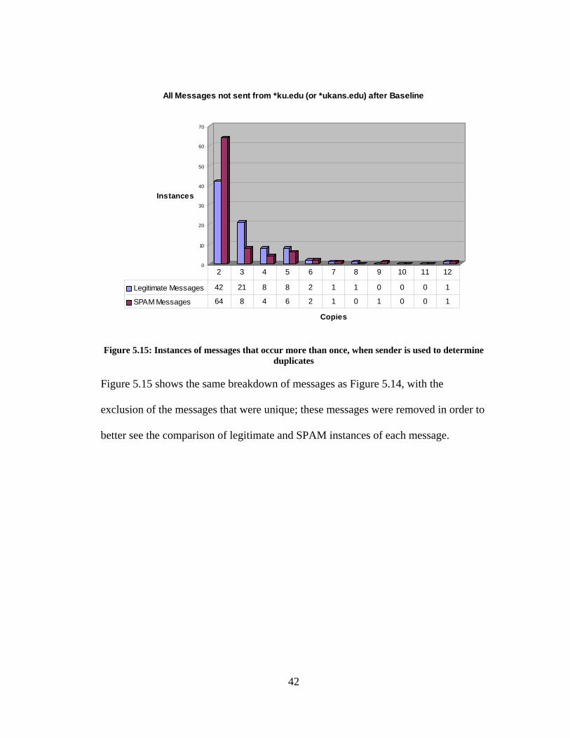
Figure 5.15: Instances of messages that occur more than once, when sender is used to determine
duplicates
Figure 5.15 shows the same breakdown of messages as Figure 5.14, with the
exclusion of the messages that were unique; these messages were removed in order to
better see the comparison of legitimate and SPAM instances of each message.
42
Precision, Recall and F-Measure
0.00
0.20
0.40
0.60
0.80
1.00
1.20
C o p ies
Recall 0.322 0.533 0.713 0.796 0.893 0.929 0.947 0.970 0.970 0.970 0.970
Precision 0.304 0.330 0.383 0.402 0.420 0.423 0.427 0.433 0.428 0.428 0.428
F-M easure 0.319 0.474 0.608 0.666 0.729 0.749 0.761 0.777 0.774 0.774 0.774
2 3 4 5 6 7 8 9 10 11 12
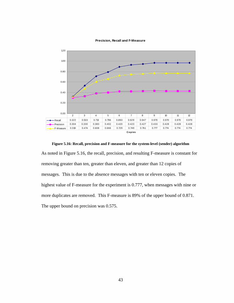
Figure 5.16: Recall, precision and F-measure for the system-level (sender) algorithm
As noted in Figure 5.16, the recall, precision, and resulting F-measure is constant for
removing greater than ten, greater than eleven, and greater than 12 copies of
messages. This is due to the absence messages with ten or eleven copies. The
highest value of F-measure for the experiment is 0.777, when messages with nine or
more duplicates are removed. This F-measure is 89% of the upper bound of 0.871.
The upper bound on precision was 0.575.
43
Accuracy
0.00
0.10
0.20
0.30
0.40
0.50
0.60
0.70
0.80
0.90
1.00
C o p ies
Inst
ance
s
Accuracy 0.385 0.329 0.377 0.398 0.418 0.418 0.425 0.435 0.424 0.424 0.424
2 3 4 5 6 7 8 9 10 11 12
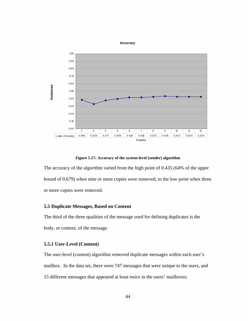
Figure 5.17: Accuracy of the system-level (sender) algorithm
The accuracy of the algorithm varied from the high point of 0.435 (64% of the upper
bound of 0.679) when nine or more copies were removed, to the low point when three
or more copies were removed.
5.5 Duplicate Messages, Based on Content
The third of the three qualities of the message used for defining duplicates is the
body, or content, of the message.
5.5.1 User-Level (Content)
The user-level (content) algorithm removed duplicate messages within each user’s
mailbox. In the data set, there were 747 messages that were unique to the users, and
15 different messages that appeared at least twice in the users’ mailboxes.
44
0
50
100
150
200
250
300
350
400
450
Instances
Copies
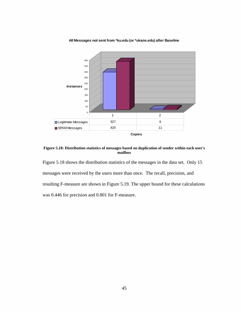
All Messages not sent from *ku.edu (or *ukans.edu) after Baseline
Legitimate Messages 327 6
SPAM Messages 420 11
1 2
Figure 5.18: Distribution statistics of messages based on duplication of sender within each user's
mailbox
Figure 5.18 shows the distribution statistics of the messages in the data set. Only 15
messages were received by the users more than once. The recall, precision, and
resulting F-measure are shown in Figure 5.19. The upper bound for these calculations
was 0.446 for precision and 0.801 for F-measure.
45
Precision vs. Recall
0.00
0.20
0.40
0.60
0.80
1.00
1.20
Copies
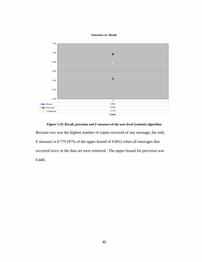
Recall 0.967
Precision 0.438
F-Measure 0.779
2
Figure 5.19: Recall, precision and F-measure of the user-level (content) algorithm
Because two was the highest number of copies received of any message, the only
F-measure is 0.779 (97% of the upper bound of 0.801) when all messages that
occurred twice in the data set were removed. The upper bound for precision was
0.446.
46
Accuracy
0.00
0.10
0.20
0.30
0.40
0.50
0.60
0.70
0.80
0.90
1.00
Copies
Inst
ance
s
Accuracy 0.447
2
Figure 5.20: Accuracy of the user-level (content) algorithm
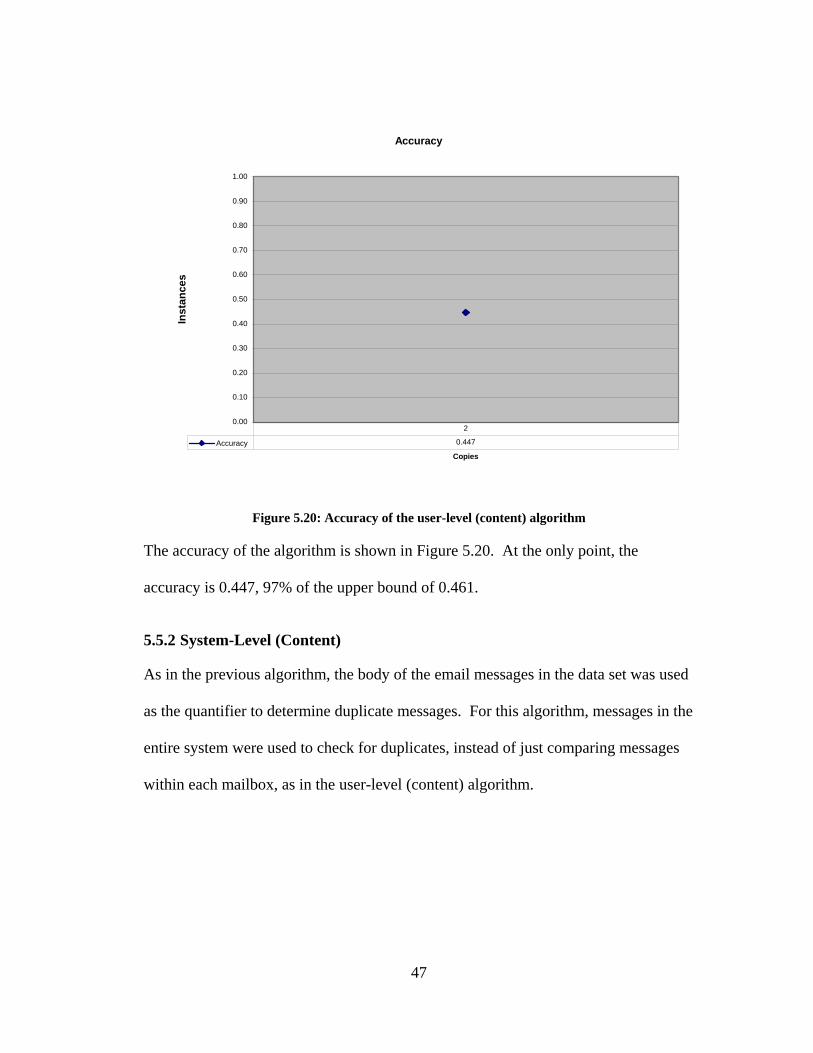
The accuracy of the algorithm is shown in Figure 5.20. At the only point, the
accuracy is 0.447, 97% of the upper bound of 0.461.
5.5.2 System-Level (Content)
As in the previous algorithm, the body of the email messages in the data set was used
as the quantifier to determine duplicate messages. For this algorithm, messages in the
entire system were used to check for duplicates, instead of just comparing messages
within each mailbox, as in the user-level (content) algorithm.
47
0
50
100
150
200
250
300
350
Instances
Copies
All Messages not sent from *ku.edu (or *ukans.edu) after Baseline
Legitimate Messages 276 27 4 0 0
SPAM Messages 350 37 5 1 1
1 2 3 4 5
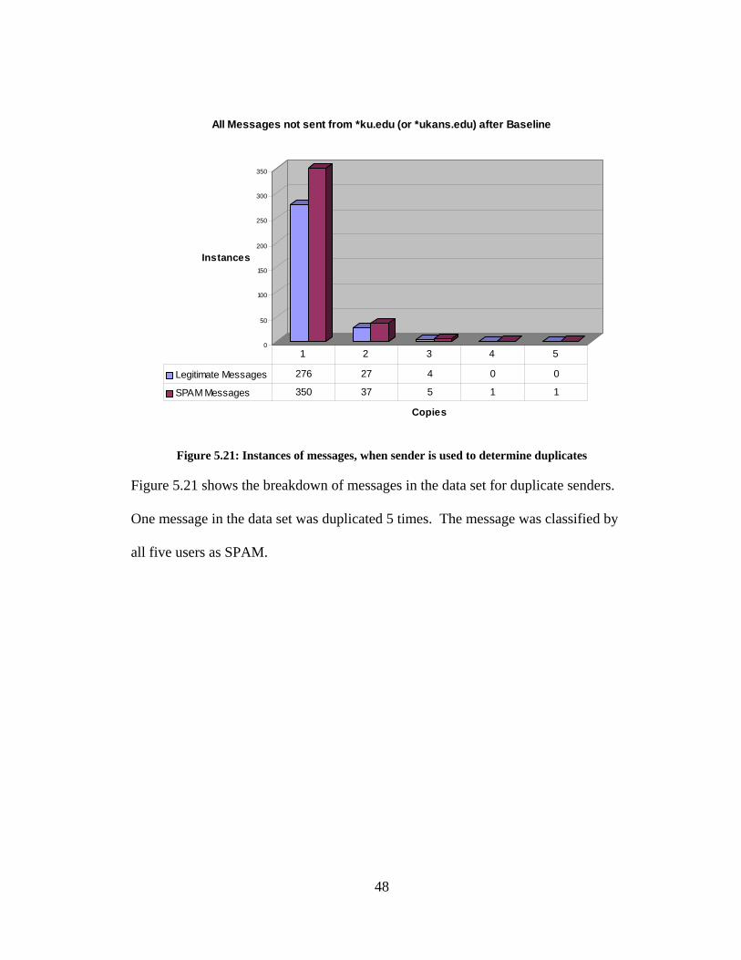
Figure 5.21: Instances of messages, when sender is used to determine duplicates
Figure 5.21 shows the breakdown of messages in the data set for duplicate senders.
One message in the data set was duplicated 5 times. The message was classified by
all five users as SPAM.
48
Precision, Recall and F-Measure
0.00
0.20
0.40
0.60
0.80
1.00
1.20
C o p ies
Recall 0.817 0.973 1.000 1.000
Precision 0.441 0.438 0.439 0.437
F-M easure 0.698 0.782 0.796 0.795
2 3 4 5
Figure 5.22: Recall, precision and F-measure for the system-level (content) algorithm
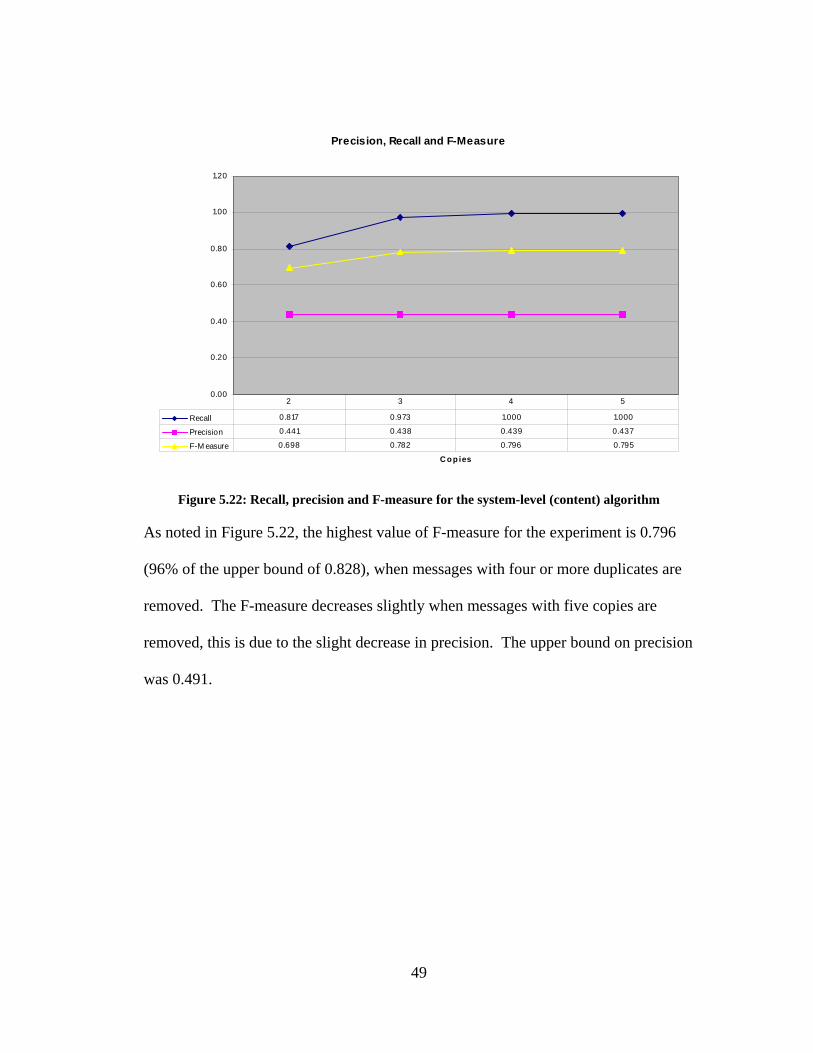
As noted in Figure 5.22, the highest value of F-measure for the experiment is 0.796
(96% of the upper bound of 0.828), when messages with four or more duplicates are
removed. The F-measure decreases slightly when messages with five copies are
removed, this is due to the slight decrease in precision. The upper bound on precision
was 0.491.
49
Accuracy
0.00
0.10
0.20
0.30
0.40
0.50
0.60
0.70
0.80
0.90
1.00
C o p ies
Inst
ance
s
Accuracy 0.471 0.445 0.445 0.440
2 3 4 5
Figure 5.23: Accuracy of the system-level (content) algorithm
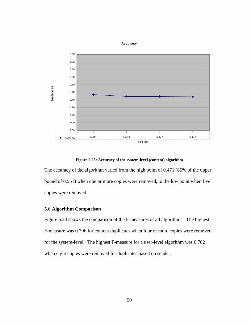
The accuracy of the algorithm varied from the high point of 0.471 (85% of the upper
bound of 0.551) when one or more copies were removed, to the low point when five
copies were removed.
5.6 Algorithm Comparison
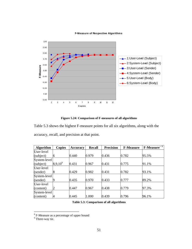
Figure 5.24 shows the comparison of the F-measures of all algorithms. The highest
F-measure was 0.796 for content duplicates when four or more copies were removed
for the system-level. The highest F-measure for a user-level algorithm was 0.782
when eight copies were removed for duplicates based on sender.
50
F-Measure of Respective Algorithms
0.00
0.10
0.20
0.30
0.40
0.50
0.60
0.70
0.80
0.90
1.00
2 3 4 5 6 7 8 9 10 11 12
C o p ies
F-M
easu
re
1:User-Level (Subject)2:System-Level (Subject)3:User-Level (Sender)4:System-Level (Sender)5:User-Level (Body)6:System-Level (Body)
Figure 5.24: Comparison of F-measures of all algorithms
Table 5.3 shows the highest F-measure points for all six algorithms, along with the
accuracy, recall, and precision at that point.
Algorithm Copies Accuracy Recall Precision F-Measure F-Measure` 8
User-level (subject) 6 0.440 0.979 0.436 0.782 95.5% System-level (subject) 8,9,109 0.431 0.967 0.431 0.775 91.1% User-level (sender) 8 0.429 0.982 0.431 0.782 93.1% System-level (sender) 9 0.435 0.970 0.433 0.777 89.2% User-level (content) 2 0.447 0.967 0.438 0.779 97.3% System-level (content) 4 0.445 1.000 0.439 0.796 96.1%
Table 5.3: Comparison of all algorithms
8 F-Measure as a percentage of upper bound 9 Three-way tie.
51
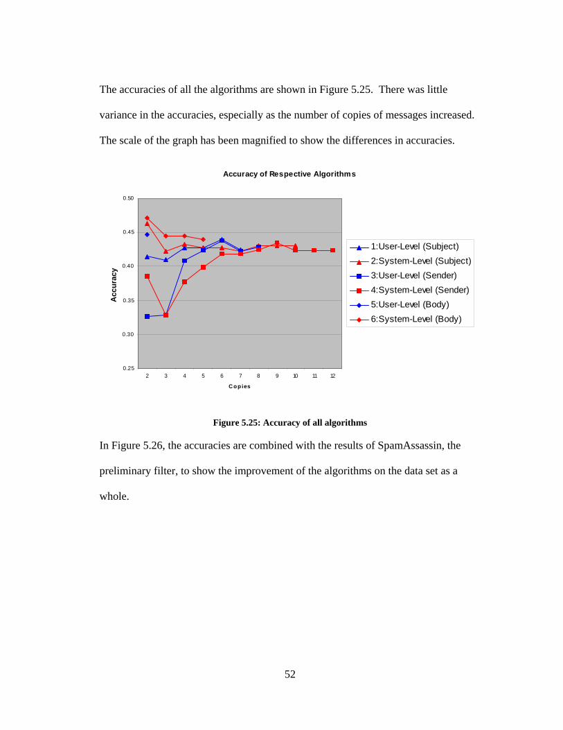
The accuracies of all the algorithms are shown in Figure 5.25. There was little
variance in the accuracies, especially as the number of copies of messages increased.
The scale of the graph has been magnified to show the differences in accuracies.
Accuracy of Respective Algorithms
0.25
0.30
0.35
0.40
0.45
0.50
2 3 4 5 6 7 8 9 10 11 12
C o p ies
Acc
urac
y
1:User-Level (Subject)2:System-Level (Subject)3:User-Level (Sender)4:System-Level (Sender)5:User-Level (Body)6:System-Level (Body)
Figure 5.25: Accuracy of all algorithms
In Figure 5.26, the accuracies are combined with the results of SpamAssassin, the
preliminary filter, to show the improvement of the algorithms on the data set as a
whole.
52
Accuracy of Respective Algorithms
-0.030
-0.020
-0.010
0.000
0.010
0.020
0.030
2 3 4 5 6 7 8 9 10 11 12
C o p ies
Acc
urac
y Im
prov
emen
t ove
r Sp
amA
ssas
sin
1: User-Level (Subject)2:System-Level (Subject)3:User-Level (Sender)4:System-Level (Sender)5:User-Level (Body)6:System-Level (Body)
Figure 5.26: Accuracies of algorithms when combined with SpamAssassin
The two algorithms based on content duplicates are the only algorithms that
consistently improve on SpamAssassin alone. The user-level algorithms based on
subject and sender duplication each have one point above SpamAssassin, both when
six copies or more of messages are removed.
5.7 Discussion
As the number of copies of each message increased, the recall and the resulting
F-measures for the algorithms increased. This proves that the probability of a
message to be SPAM increases as the number of copies of the messages increases.
It is hard to determine the overall best algorithm, or if user-level or system-level
filtering was more effective. The highest performing user-level algorithm was the
53
user-level (sender) algorithm. The highest performing system-level algorithm was
the system-level (content) algorithm. Since all algorithms improve with more
duplicates, a larger collection of participating users in our study would likely have
shown more convincing improvements. Similarly, if deployed on the server for all
users in a large organization, the increased number of duplicates might render this an
effective second-level filtering technique.
54
Chapter 6: Validation
The two algorithms with the highest F-measures were tested using e-mails from a
second, consecutive week of e-mail received by the same users.
After the void messages, and intra-server e-mail were removed, the validation set
contained 4,055 messages, 3,272 of which SpamAssassin tagged as SPAM, as seen in
Table 6.1. SpamAssassin tagged one message as SPAM that a user classified as
valid, resulting in one false positive.
Tagged as
Legitimate Tagged as SPAM
Legitimate According to User
288 1
SPAM According to User 495 3271
Table 6.1: Confusion matrix for SpamAssassin preliminary filter on Validation Set
Table 6.2 shows the performance of SpamAssassin, including a lower F-measure than
before of 0.743. All messages classified as SPAM by SpamAssassin were removed
from the validation set.
Accuracy SPAM
Missed Legitimate
Tagged Recall Precision F-measure
SpamAssassin 87.7% 12.2% 0.0002% 99.6% 36.8% 0.743
Table 6.2: SpamAssassin Statistics on Test Data Set
The remaining 783 messages were used to re-evaluate the system-level (content)
algorithm, and the user-level (sender) algorithm. Two-hundred eighty-eight of the
messages were legitimate, and 495 were SPAM.
55
Precision, Recall and F-Measure
0.00
0.20
0.40
0.60
0.80
1.00
1.20
Copies
Recall 0.817 0.973 1.000 1.000
Precision 0.441 0.438 0.439 0.437
F-Measure 0.698 0.782 0.796 0.795
Recall' 0.760 0.983 0.997 0.997 0.997
Precision' 0.375 0.377 0.369 0.369 0.369
F-Measure' 0.631 0.744 0.744 0.744 0.744
2 3 4 5 6
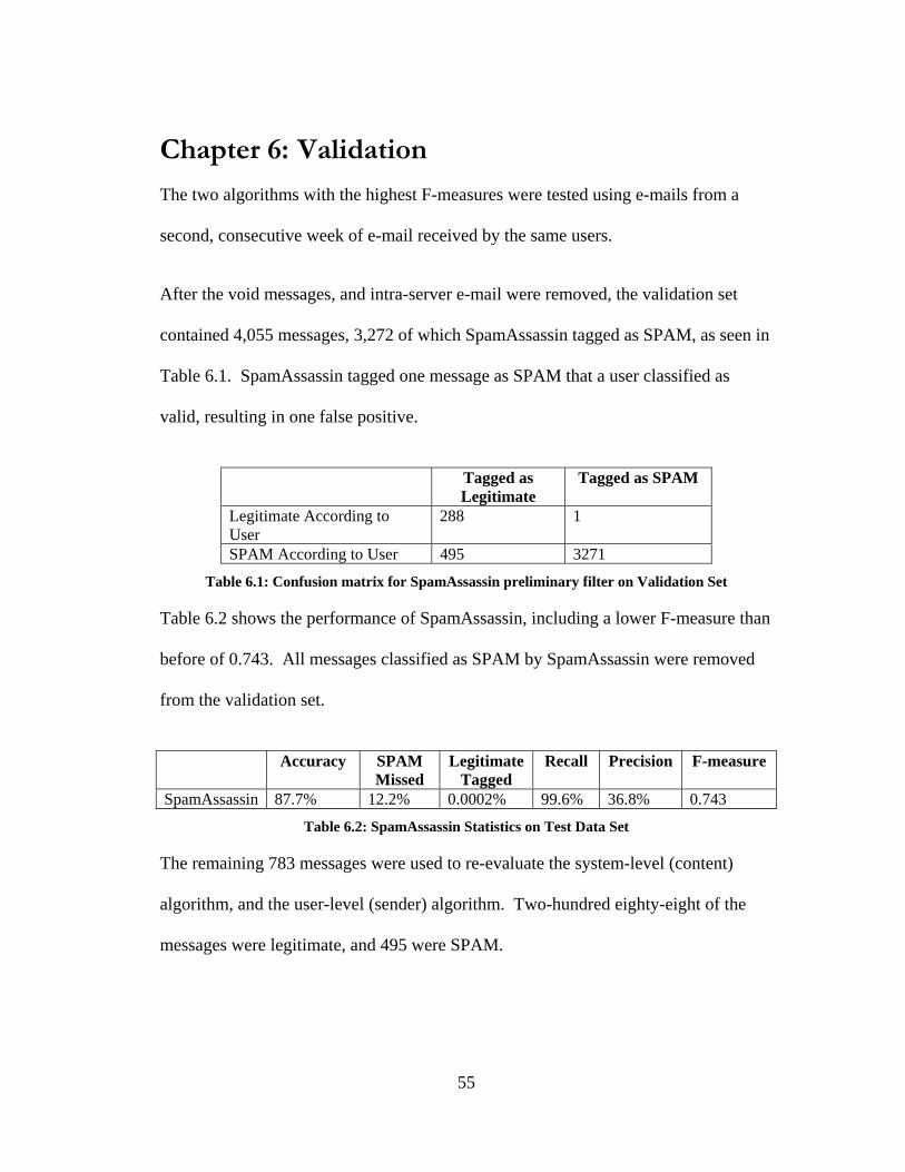
Figure 6.1: Validation of the system-level (content) algorithm: Precision, Recall and F-Measure
For the system-level (content) algorithm, the validation resulted in lower F-measures
across the board. The highest F-measure of 0.7444 was 93.2% of the upper bound of
0.798. This number was 0.052 less than the highest F-measure when the algorithm
was run on the data set, and 3% lower in relation to each experiment’s upper bound.
The patterning is almost identical, which validates the consistency of this algorithm.
56
Accuracy
0.00
0.10
0.20
0.30
0.40
0.50
0.60
0.70
0.80
0.90
1.00
Copies
Inst
ance
s
Accuracy 0.471 0.445 0.445 0.440
Accuracy' 0.446 0.397 0.373 0.373 0.373
2 3 4 5 6
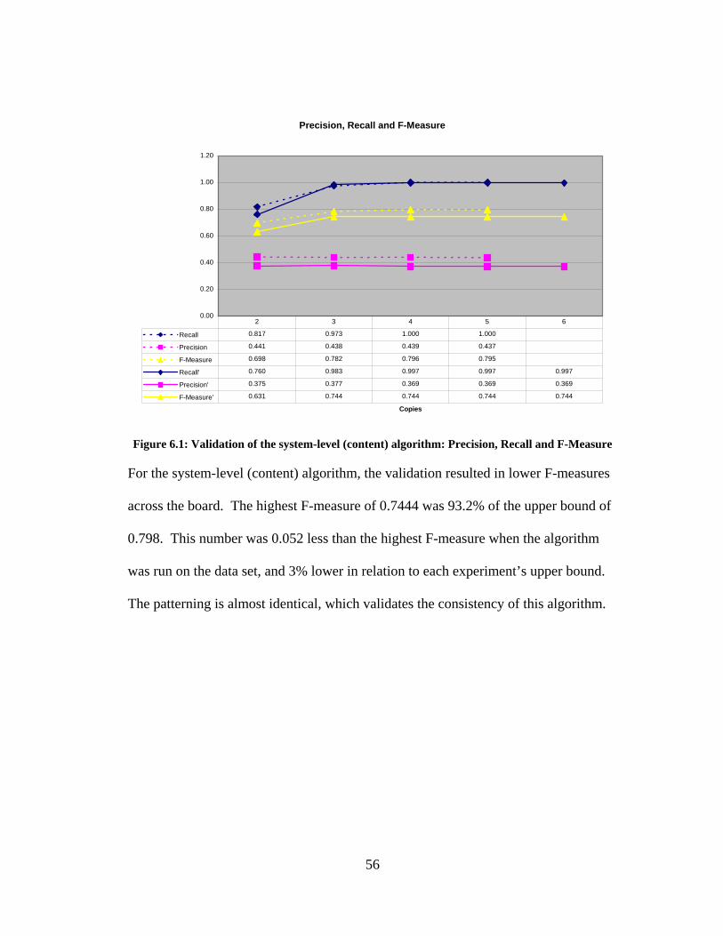
Figure 6.2: Accuracy of the system-level (content) algorithm: test data versus validation data set
The accuracy was also slightly lower. The high point of the validation accuracy was
0.446, 84% of the upper bound. The accuracy is 0.004 less than the same accuracy
point for the data set. Again, the patterning is similar for both accuracies, with a high
point when removing two or more copies of messages, and a slightly decreasing
accuracy for points after that.
57
Precision, Recall and F-Measure
0.00
0.20
0.40
0.60
0.80
1.00
1.20
C o p ies
Recall 0.399 0.595 0.837 0.896 0.964 0.964 0.982
Precision 0.295 0.342 0.411 0.423 0.434 0.427 0.431
F-M easure 0.373 0.518 0.693 0.732 0.775 0.770 0.782
Recall' 0.378 0.628 0.691 0.788 0.868 0.917 0.917 0.924 0.938 0.938 0.938 0.979 0.979 0.979
Precision' 0.242 0.317 0.320 0.337 0.353 0.357 0.357 0.356 0.357 0.357 0.357 0.367 0.367 0.367
F-M easure' 0.340 0.525 0.561 0.622 0.672 0.698 0.698 0.700 0.708 0.708 0.708 0.734 0.734 0.734
2 3 4 5 6 7 8 9 10 11 12 13 14 15
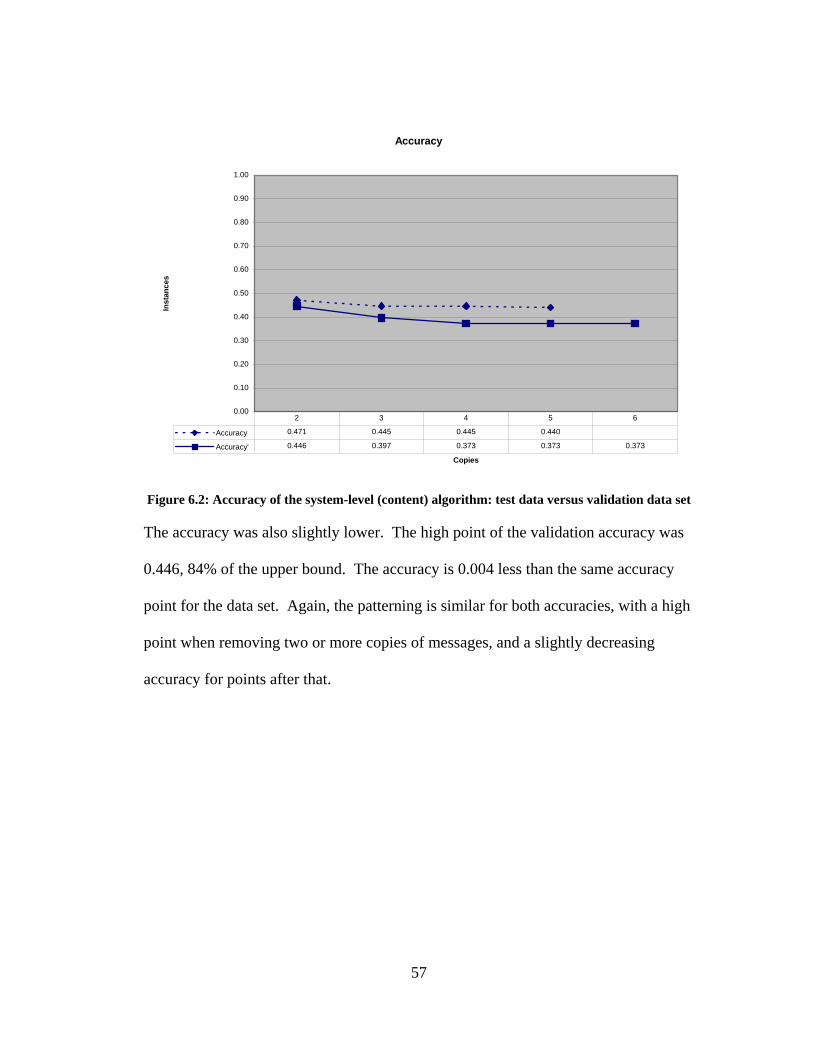
Figure 6.3: Comparison of Precision, Recall and F-Measure for the user-level (sender) algorithm
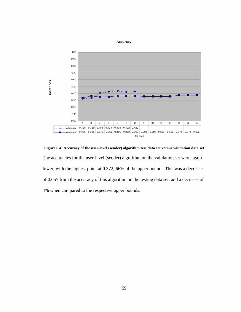
For the user-level (sender) algorithm, F-measures were on average 0.05 lower. The
highest F-measure of 0.734 was 91% of the upper bound of 0.808. The patterning of
recall, precision, and F-measure are closely related, resulting in a similar increase in
the algorithm as higher quantity copies are removed from each data set.
58
Accuracy
0.00
0.10
0.20
0.30
0.40
0.50
0.60
0.70
0.80
0.90
1.00
C o p ies
Inst
ance
s
Accuracy 0.326 0.329 0.408 0.424 0.438 0.422 0.429
Accuracy' 0.335 0.365 0.346 0.351 0.365 0.363 0.363 0.358 0.356 0.356 0.356 0.372 0.372 0.372
2 3 4 5 6 7 8 9 10 11 12 13 14 15
Figure 6.4: Accuracy of the user-level (sender) algorithm test data set versus validation data set
The accuracies for the user-level (sender) algorithm on the validation set were again
lower, with the highest point at 0.372, 66% of the upper bound. This was a decrease
of 0.057 from the accuracy of this algorithm on the testing data set, and a decrease of
4% when compared to the respective upper bounds.
59
Chapter 7: Conclusions and Future Work
Overall, the algorithms performed as well or better than predicted. When the body, or
content, of a message is used as the measure for duplication, the results are along the
lines of what was expected for all of the filters.
Several unforeseen items led to low performance scores. Only dealing with duplicate
messages limited the overall effectiveness. There were more unique SPAM
messages, and more duplicate legitimate messages, than predicted before the data
collection began. This limited the degree of precision, and resulting F-measure that
was possible for each algorithm. On average, the algorithms performed 90% or better
as compared to the maximum achievable F-measure. When combined with a
preliminary filter such as SpamAssassin, these algorithms proved some worth,
although would be ineffective as a stand-alone filter.
Other factors contributed to low performance scores. One major issue is the training
data set. In these experiments, real e-mails classified by humans were used. This
seems like the only way to gather a data set, when the filter is built to classify real
e-mail, however, since there were sixteen users classifying the messages
independently, this created a problem. Often times a message would be classified as
SPAM and legitimate by two different users, sometimes classified as SPAM and
legitimate by the same user. This proves that SPAM is subjective, and a more
personalized filter might be a better solution.
60
Other future enhancements may be the introduction of a learning system within the
collaborative filter. In a learning system, the filter could red flag duplicates, and then
monitor how each user classified the message, and predict how the other users would
react. For example, if five people received the same message, and user 1 classified it
as SPAM, the system might assume the other four copies as SPAM. However, if user
2 classified the message as legitimate, the filter may change the classification to
legitimate. Some algorithm would be applied to make this judgment, most likely a set
number of judgments would have to be received from the users, and then looking at
the majority of the judgments, the filter would make a decision. Vipul’s Razor [18],
mentioned above, uses a variation of this, allowing users from all over the world to
report SPAM messages to a centralized clearinghouse. The model proposed above
would be automated, and would most likely be specific to one ISP or one corporation.
61
Bibliography
[1] Androutsopoulos, J. Koutsias, K. V. Chandrinos, G. Paliouras, and C. D.
Spyropoulos. An Evaluation of Naïve Bayesian Anti-Spam Filtering. In Proc. of the
Workshop on Machine Learning in the New Information Age, 2000.
[2] I. Androutsopoulos, G. Paliouras, V. Karkaletsis, G. Sakkis, C. Spyropoulos, and
P. Stamatopoulos. Learning to Filter SPAM E-Mail: A Comparison of a Naïve
Bayesian and a Memory-Based approach. In Workshop on Machine Learning and
Textual Information Access, 4th European Conference on Principles and Practice of
Knowledge Discovery in Databases, 2000.
[3] Billsus, D. and Pazzani, M. J. Learning Collaborative Information Filters. In
Proceedings of the Fifteenth International Conference on Machine Learning, pp. 46–
54, Madison, WI, 1998.
[4] Breese, J. S., Heckerman, D., Kadie, C. Empirical Analysis of Predictive
Algorithms for Collaborative Filtering. In Proceedings of the Fourteenth Annual
Conference on Uncertainty in Artificial Intelligence, pp. 43–52, July 1998.
[5] Cohen, William W. Fast Effective Rule Induction. In Machine Learning:
Proceedings of the Twelfth International Conference, Lake Tahoe, California, 1995.
[6] Cohen, William, W. Learning Rules that Classify E-Mail. In Papers from the
AAAI Spring Symposium on Machine Learning in Information Access, 18–25, 1996.
62
[7] P. Cunningham, N. Nowlan, S. J. Delany, and M. Haahr. A Case-Based Approach
to SPAM Filtering that can Track Concept Drift. In The ICCBR'03 Workshop on
Long-Lived CBR Systems, Trondheim, Norway, June 2003.
[8] Daelemans, W., Z. Jakub, K. van der Sloot and A. van den Bosch. 1999. TiMBL:
Tilburg Memory Based Learner, version 2.0, Reference Guide. ILK, Comutational
Linguistics, Tilburg University.
[9] Federal Trade Commission: Federal, State, and Local Law Enforcers Tackle
Deceptive Spam and Internet Scams. http://www.ftc.gov/opa/2002/11/netforce.htm,
November 13, 2002.
[10] Garcia, F. D., J.-H. Hoepman, and J. van Nieuwenhuizen. Spam Filter Analysis.
Proceedings of 19th IFIP International Information Security Conference, WCC2004-
SEC, 2004.
[11] Madigan, D. Statistics and the War on Spam, Statistics, A Guide to the
Unknown, 2004.
[12] Open Relay Database. http://ordb.org.
[13] Rucker, J. and Polanco, M.J. SiteSeer: Personalized Navigation of the Web.
Communications of the ACM, 40(3):73–75, 1997.
63
[14] Sahami, M., Dumais, S., Heckerman, D., and Horvitz, E. A Bayesian Approach
to Filtering Junk E-Mail. In Learning for Text Categorization - Papers from the AAAI
Workshop, pp. 55–62, Madison Wisconsin. AAAI Technical Report WS-98-05, 1998.
[15] Salton, G. Developments in Automatic Text Retrieval. Science, 253:974–980,
1991.
[16] SPAMCOP Blacklist. http://www.spamcop.net/bl.shtml.
[17] Sullivan, B. Now, two-thirds of all e-mail is SPAM.
http://www.msnbc.msn.com/id/5032714/, May 22, 2004.
[18] Vipul’s Razor. http://razor.sourceforge.net, 2005.
64