École de technologie supÉrieure universitÉ du quÉbec ... · board of examiners this thesis has...
TRANSCRIPT

ÉCOLE DE TECHNOLOGIE SUPÉRIEURE
UNIVERSITÉ DU QUÉBEC
THESIS PRESENTED TO
ÉCOLE DE TECHNOLOGIE SUPÉRIEURE
IN PARTIAL FULFILLMENT OF THE REQUIREMENTS FOR
A MASTER’S DEGREE IN MECHANICAL ENGINEERING
M.A.Sc.
BY
Cédrik BACON
MEASUREMENT, MODELLING AND SIMULATION OF EARPHONE SOUND
SIGNATURE
MONTREAL, “SEPTEMBER 20TH 2013”
© Copyright 2013 reserved by Cédrik BACON

© Copyright reserved
It is forbidden to reproduce, save or share the content of this document either in whole or in parts. The reader
who wishes to print or save this document on any media must first get the permission of the author.

BOARD OF EXAMINERS
THIS THESIS HAS BEEN EVALUATED
BY THE FOLLOWING BOARD OF EXAMINERS:
Dr. Jérémie Voix, Memorandum Director
Mechanical Engineering Department, École de technologie supérieure
Dr. Ghyslain Gagnon, Committee President
Electrical Engineering Department, École de technologie supérieure
Dr. Frédéric Laville, Examiner
Mechanical Engineering Department, École de technologie supérieure
Dr. Sean E. Olive, External Examiner
Director Acoustic Research, Harman International
Mr. Michael C. Turcot, External Examiner
Vice-President, Manufacturing, R & D, Sonomax Technologies Inc.
THIS THESIS WAS PRESENTED AND DEFENDED
IN THE PRESENCE OF A BOARD OF EXAMINERS AND PUBLIC
ON ”SEPTEMBER 10TH 2013”
AT ÉCOLE DE TECHNOLOGIE SUPÉRIEURE


ACKNOWLEDGEMENTS
"There is something beautiful about stating the obvious. All of us do it in those moments where
we can’t believe that we have to say it. It’s like pinching yourself to make sure you are awake."
- Shane Koyczan
After so many years, the time has come to take a moment to write in (electronic) ink a special
word of thanks to those who made a difference in my life. The best math teacher, and my soon-
to-be-wife, Émilie who supported me, as always, in this endeavour. Claude et Gabriel, maman
et papa, qui croient que l’éducation est le plus beau cadeau que l’on puisse faire à quelqu’un.
Et qui ont certainement raison. To all the friends and family who made a difference over the
years: life is better enjoyed with wonderful people to enjoy it with.
Also, a special thanks to Frédéric Laville, a fantastic professor who made it possible to consider
acoustics as more than just a hobby and to Jérémie Voix, who made it possible to make a career
out of it! To the very generous Michael "Mike" Turcot, thanks for that walk in Toronto under
freezing rain and for all those long drives back and forth on the 401. You are an inspiration and
an example to follow. It is true what they say, the most important thing is not the destination
but the journey and those with whom you are travelling.
To the many others at Sonomax and at the Sonomax-ÉTS Industrial Research Chair in In-Ear
Technologies (CRITIAS), thank you as well. This entire experience would not have been the
same without you!
And last but not least, Antoine Bernier, who made the daily writing of this thesis a merrier and
better experience. Cheers Antoine!
*This work was funded and supported by Sonomax Technologies Inc. in partnership with Le
Fonds de recherche du Québec – Nature et technologies (FRQNT) and the Natural Sciences
and Engineering Research Council of Canada (NSERC).

MEASUREMENT, MODELLING AND SIMULATION OF EARPHONE SOUNDSIGNATURE
Cédrik BACON
ABSTRACT
Earphones are no longer a novelty or substandard to large sound systems. People use them for
music reproduction, on the go and even at home. However, the frequency responses of the ear-
phones nowadays available are as different as the exterior designs of the earpieces. This master
thesis aims at identifying the contributing factors, from a psycho-acoustics point of view, to a
good sound signature for earphones. It also presents the components necessary to achieve such
a sound signature from a design point of view. To do so, this thesis presents an important liter-
ature review and highlights an issue not present when sound reproduction is performed with a
distant source: the variability of the coupling between the ear and the earphone. In a first part,
the psycho-acoustics of listening with earphones is explained because earphones do not pro-
vide important cues that listeners would naturally perceive when listening to a distant source.
Various perceptual audio descriptors such as loudness, frequency response and other metrics
are also presented in order to establish the requirements for earphone design. In a second part,
the measurement of earphones and the measurement tools available to these measurement are
presented. The concept of electrical impedance, frequency response and distortion measure-
ment are covered. The reliability of these tools as indicators of the variability of the coupling
between the ear and the earphone for a given population is compiled from various published
studies. In a third part several modelling methods, such as the lumped-elements, control-system
block diagrams and two-port networks, are detailed and the models of electro-acoustic trans-
ducers and passive components are covered. A simulation is performed on earphones recently
developed by the industrial partner of this work with software tools like MATLAB®, Simulink®
and Simscape®. Lastly, this thesis presents areas identified during this research that would ben-
efit from further research, such as the need for a new broad-band measurement apparatus and
the need for psycho-acoustic studies on the impact of the coupling between the ear and the ear-
phone. A practical solution to the delicate question of the earphone/ear coupling variability is
offered and relies on the automated and individualized adjustment of the earphones frequency
response based on the measurement -by the digital audio player- of the electrical impedance of
the earphones.
Keywords: acoustics, electro-acoustics, psycho-acoustics, product development, percep-
tual audio, headphones, earphones, loudspeaker, modelling, design, two-port,
lumped-element, loudness, simulation, innovation theory, measurement

MEASUREMENT, MODELLING AND SIMULATION OF EARPHONE SOUNDSIGNATURE
Cédrik BACON
RÉSUMÉ
Les écouteurs ne sont plus une nouveauté ou une alternative bon marché à des systèmes de
reproduction sonore dits de salon. Ils sont maintenant utilisés pour écouter de la musique
autant en déplacement qu’à la maison. Cependant, les réponses en fréquence des écouteurs
disponibles actuellement sont aussi différentes que leurs designs extérieurs. Ce mémoire vise
à identifier les facteurs qui contribuent, du point de vue de la psychoacoustique, à une bonnesignature sonore pour un écouteur donné. Il présente également les composantes nécessaires à
la réalisation d’une telle signature sonore d’un point de vue de la conception. Pour ce faire, une
importante revue de la littérature est produite et met en évidence l’effet de la variabilité du cou-
plage entre l’écouteur et l’oreille. Dans un premier temps, les aspects psychoacoustiques pro-
pres aux écouteurs sont présentés étant donné que les écouteurs ne fournissent pas des indices
sonores qu’un sujet reçoit habituellement lors de l’écoute de sources distantes. Une présen-
tation est faite de plusieurs descripteurs perceptifs tels que la sonie, la réponse en fréquence
et d’autres métriques nécessaires à la mise en place des requis de base pour la conception
d’écouteurs. Dans un deuxième temps, les méthodes de mesure des écouteurs ainsi que les out-
ils disponibles pour ces mesures sont passés en revue. L’impédance électrique, la réponse en
fréquence et la mesure de la distorsion sont ainsi présentées en détail. La fiabilité de ces outils
comme des indicateurs de la variabilité du couplage entre l’oreille et l’écouteur pour une popu-
lation donnée est analysée à travers une synthèse de diverses études publiées. Dans un troisième
temps plusieurs approches de modélisation sont présentées, notamment celle par éléments lo-
calisés, celle des schémas de contrôle de système et celle des quadripôles, et les modèles des
transducteurs électroacoustiques et des composants électriques passifs sont rappelés. Une sim-
ulation de plusieurs écouteurs récemment commercialisés par le partenaire industriel de ce pro-
jet est par la suite faite à l’aide des outils logiciels MATLAB®, Simulink® et Simscape®. Pour
terminer, ce mémoire identifie des domaines qui pourraient bénéficier d’avantage de recherche,
à savoir de nouveaux appareils de mesure large-bande et des études psychoacoustiques sur
l’impact du couplage entre l’oreille et l’écouteur. Parallèlement, une solution pratique à la déli-
cate question de la variabilité dans le couplage écouteur/oreille est proposée et s’appuie sur
le réglage automatisé et individualisé de la réponse en fréquence des écouteurs à l’aide d’une
mesure -par le lecteur audionumérique- de l’impédance électrique des écouteurs.
Mot-clés : Acoustique, électro-acoustique, psycho-acoustique, dévelopement de produit,
audio perceptuel, écouteurs, haut-parleurs, modélisation, conception, bi-porte,
quadripôle, loudness, simulation, mesure

Contents
Page
INTRODUCTION . . . . . . . . . . . . . . . . . . . . . . . . . . . . . . . . . . . . . . . . . . . . . . . . . . . . . . . . . . . . . . . . . . . . . . . . . . . . . . . . 1
CHAPTER 1 ACOUSTICS AND PSYCHO-ACOUSTICS OF EARPHONES . . . . . . . . . . . 5
1.1 Specificities of hearing sound emitted by a distant source versus with
earphones . . . . . . . . . . . . . . . . . . . . . . . . . . . . . . . . . . . . . . . . . . . . . . . . . . . . . . . . . . . . . . . . . . . . . . . . . . . . . . . . . 7
1.1.1 Overview of the hearing process . . . . . . . . . . . . . . . . . . . . . . . . . . . . . . . . . . . . . . . . . . . . . . 7
1.1.2 Hearing a distant source: Sound paths, room reflections and the
Head-Related Transfer Function (HRTF) . . . . . . . . . . . . . . . . . . . . . . . . . . . . . . . . . . . . . 9
1.1.2.1 Sound paths and room reflections . . . . . . . . . . . . . . . . . . . . . . . . . . . . . . . . . 9
1.1.2.2 Head Related Transfer Function . . . . . . . . . . . . . . . . . . . . . . . . . . . . . . . . . . 11
1.1.3 Hearing with earphones . . . . . . . . . . . . . . . . . . . . . . . . . . . . . . . . . . . . . . . . . . . . . . . . . . . . . . . 16
1.1.4 Coupling of the earphone with the ear . . . . . . . . . . . . . . . . . . . . . . . . . . . . . . . . . . . . . . . 19
1.2 Measuring the sound quality of earphones . . . . . . . . . . . . . . . . . . . . . . . . . . . . . . . . . . . . . . . . . . . . . 21
1.2.1 Objective measurement of sound quality . . . . . . . . . . . . . . . . . . . . . . . . . . . . . . . . . . . . 21
1.2.1.1 Acoustic test fixture . . . . . . . . . . . . . . . . . . . . . . . . . . . . . . . . . . . . . . . . . . . . . . . 22
1.2.1.2 Probe microphone . . . . . . . . . . . . . . . . . . . . . . . . . . . . . . . . . . . . . . . . . . . . . . . . . 22
1.2.2 Subjective measurement of sound quality . . . . . . . . . . . . . . . . . . . . . . . . . . . . . . . . . . . 24
1.2.3 Loudness and earphone sound quality . . . . . . . . . . . . . . . . . . . . . . . . . . . . . . . . . . . . . . . 29
1.2.3.1 Just-Noticeable Sound Changes . . . . . . . . . . . . . . . . . . . . . . . . . . . . . . . . . . 31
1.2.3.2 Signal matching and loudness function . . . . . . . . . . . . . . . . . . . . . . . . . . 32
1.2.3.3 The missing 6 dB effect . . . . . . . . . . . . . . . . . . . . . . . . . . . . . . . . . . . . . . . . . . . 33
1.2.3.4 Identifying the reference recording SPL to differentiate
the proper loudness transfer function . . . . . . . . . . . . . . . . . . . . . . . . . . . . 34
1.2.4 Ear canal sealed by the earphone . . . . . . . . . . . . . . . . . . . . . . . . . . . . . . . . . . . . . . . . . . . . . 37
1.2.4.1 Increase of the Signal-to-Noise Ratio . . . . . . . . . . . . . . . . . . . . . . . . . . . . 38
1.2.4.2 Effect of sealing the ear canal on the low frequencies
reproduction . . . . . . . . . . . . . . . . . . . . . . . . . . . . . . . . . . . . . . . . . . . . . . . . . . . . . . . 39
1.3 On the definition of an earphone target frequency response . . . . . . . . . . . . . . . . . . . . . . . . . . 41
1.3.1 Issues related to earphone sound reproduction . . . . . . . . . . . . . . . . . . . . . . . . . . . . . . 41
1.3.2 Comparison of studied frequency response . . . . . . . . . . . . . . . . . . . . . . . . . . . . . . . . . . 43
1.4 Conclusions on the psycho-acoustics of earphone . . . . . . . . . . . . . . . . . . . . . . . . . . . . . . . . . . . . . 45
CHAPTER 2 MEASUREMENT OF EARPHONES: METHODOLOGY AND
DEFINITION . . . . . . . . . . . . . . . . . . . . . . . . . . . . . . . . . . . . . . . . . . . . . . . . . . . . . . . . . . . . . . . . . 49
2.1 Collocated measurement of earphones . . . . . . . . . . . . . . . . . . . . . . . . . . . . . . . . . . . . . . . . . . . . . . . . . 50
2.1.1 Application to moving-coil micro-loudspeaker . . . . . . . . . . . . . . . . . . . . . . . . . . . . . 51
2.1.2 Application to balanced-armature receivers . . . . . . . . . . . . . . . . . . . . . . . . . . . . . . . . . 55
2.2 Non-collocated measurement of earphones . . . . . . . . . . . . . . . . . . . . . . . . . . . . . . . . . . . . . . . . . . . . 55
2.2.1 Frequency Response Function . . . . . . . . . . . . . . . . . . . . . . . . . . . . . . . . . . . . . . . . . . . . . . . 57
2.2.2 Harmonic Distortion . . . . . . . . . . . . . . . . . . . . . . . . . . . . . . . . . . . . . . . . . . . . . . . . . . . . . . . . . . 60

XII
2.2.3 Intermodulation Distortion . . . . . . . . . . . . . . . . . . . . . . . . . . . . . . . . . . . . . . . . . . . . . . . . . . . 61
2.2.4 Multi-tone Distortion . . . . . . . . . . . . . . . . . . . . . . . . . . . . . . . . . . . . . . . . . . . . . . . . . . . . . . . . . 63
2.2.5 Triggered Distortion . . . . . . . . . . . . . . . . . . . . . . . . . . . . . . . . . . . . . . . . . . . . . . . . . . . . . . . . . . 64
2.2.6 Relationship between distortion and physical phenomena in a
moving-coil micro-loudspeaker . . . . . . . . . . . . . . . . . . . . . . . . . . . . . . . . . . . . . . . . . . . . . . 65
2.3 Conclusions on the measurement of earphones . . . . . . . . . . . . . . . . . . . . . . . . . . . . . . . . . . . . . . . . 66
CHAPTER 3 EARPHONE MODELLING AND SIMULATION . . . . . . . . . . . . . . . . . . . . . . . . . 69
3.1 Fundamentals of electro-acoustic modelling . . . . . . . . . . . . . . . . . . . . . . . . . . . . . . . . . . . . . . . . . . . 72
3.1.1 Impedance of physical quantities . . . . . . . . . . . . . . . . . . . . . . . . . . . . . . . . . . . . . . . . . . . . 72
3.1.2 Physical analogy of components by domain . . . . . . . . . . . . . . . . . . . . . . . . . . . . . . . . . 74
3.2 Modelling earphone-ear system coupling . . . . . . . . . . . . . . . . . . . . . . . . . . . . . . . . . . . . . . . . . . . . . . 75
3.2.1 Common methods used to describe physical systems . . . . . . . . . . . . . . . . . . . . . . . 77
3.2.1.1 Control System Block Diagram modelling method . . . . . . . . . . . . . 77
3.2.1.2 Port modelling method . . . . . . . . . . . . . . . . . . . . . . . . . . . . . . . . . . . . . . . . . . . . 79
3.2.2 Models of a human ear . . . . . . . . . . . . . . . . . . . . . . . . . . . . . . . . . . . . . . . . . . . . . . . . . . . . . . . 82
3.2.3 Models of moving-coil micro-loudspeakers . . . . . . . . . . . . . . . . . . . . . . . . . . . . . . . . . 83
3.2.3.1 Simple and complex lumped-element model . . . . . . . . . . . . . . . . . . . . 85
3.2.3.2 Two-Port model . . . . . . . . . . . . . . . . . . . . . . . . . . . . . . . . . . . . . . . . . . . . . . . . . . . 87
3.2.3.3 Block-diagram model . . . . . . . . . . . . . . . . . . . . . . . . . . . . . . . . . . . . . . . . . . . . . 87
3.2.4 Models of balanced-armature micro-loudspeakers . . . . . . . . . . . . . . . . . . . . . . . . . . 89
3.2.4.1 Lumped-elements models . . . . . . . . . . . . . . . . . . . . . . . . . . . . . . . . . . . . . . . . 90
3.2.4.2 Complex control system block-diagram model . . . . . . . . . . . . . . . . . . 91
3.2.5 Models of acoustical features found in earphones . . . . . . . . . . . . . . . . . . . . . . . . . . . 92
3.2.5.1 Acoustic mass, resistance and compliance . . . . . . . . . . . . . . . . . . . . . . . 93
3.2.5.2 Horn . . . . . . . . . . . . . . . . . . . . . . . . . . . . . . . . . . . . . . . . . . . . . . . . . . . . . . . . . . . . . . . 95
3.2.5.3 Sudden section change . . . . . . . . . . . . . . . . . . . . . . . . . . . . . . . . . . . . . . . . . . . . 97
3.2.5.4 Synthetic material membrane . . . . . . . . . . . . . . . . . . . . . . . . . . . . . . . . . . . . 97
3.2.5.5 Perforated sheets, meshes and foams . . . . . . . . . . . . . . . . . . . . . . . . . . . . 99
3.2.6 Limitations of the modelling and simulation methods . . . . . . . . . . . . . . . . . . . . .100
3.2.7 Simulation and computation method using two-port models . . . . . . . . . . . . . .101
3.3 Introduction to Design, Modelling and Simulation of Earphones with
Simulink® . . . . . . . . . . . . . . . . . . . . . . . . . . . . . . . . . . . . . . . . . . . . . . . . . . . . . . . . . . . . . . . . . . . . . . . . . . . . . . .104
3.3.1 Abstract . . . . . . . . . . . . . . . . . . . . . . . . . . . . . . . . . . . . . . . . . . . . . . . . . . . . . . . . . . . . . . . . . . . . . . .104
3.3.2 Introduction . . . . . . . . . . . . . . . . . . . . . . . . . . . . . . . . . . . . . . . . . . . . . . . . . . . . . . . . . . . . . . . . . .104
3.3.3 Description of modelling methods . . . . . . . . . . . . . . . . . . . . . . . . . . . . . . . . . . . . . . . . . .105
3.3.3.1 Ordinary Differential Equation and Differential Algebraic
Equation . . . . . . . . . . . . . . . . . . . . . . . . . . . . . . . . . . . . . . . . . . . . . . . . . . . . . . . . . .105
3.3.3.2 Lumped-Element circuit abstraction . . . . . . . . . . . . . . . . . . . . . . . . . . . .106
3.3.3.3 Control System Block Diagram . . . . . . . . . . . . . . . . . . . . . . . . . . . . . . . . .107
3.3.4 Models of acoustical components . . . . . . . . . . . . . . . . . . . . . . . . . . . . . . . . . . . . . . . . . . .109
3.3.4.1 Model of an Acoustic Mass (MA) . . . . . . . . . . . . . . . . . . . . . . . . . . . . . . .109
3.3.4.2 Model of an Acoustic Compliance (CA) . . . . . . . . . . . . . . . . . . . . . . . .110
3.3.4.3 Model of Acoustic Resistance (RA) . . . . . . . . . . . . . . . . . . . . . . . . . . . . .111

XIII
3.3.4.4 Models of Moving Coil Micro-Loudspeakers . . . . . . . . . . . . . . . . . .112
3.3.4.5 Balanced Armature Micro-Loudspeakers . . . . . . . . . . . . . . . . . . . . . . .113
3.3.4.6 Ear Simulator Model . . . . . . . . . . . . . . . . . . . . . . . . . . . . . . . . . . . . . . . . . . . . .114
3.3.5 Simulation with Simulink® . . . . . . . . . . . . . . . . . . . . . . . . . . . . . . . . . . . . . . . . . . . . . . . . . .115
3.3.6 Selection of a Solver . . . . . . . . . . . . . . . . . . . . . . . . . . . . . . . . . . . . . . . . . . . . . . . . . . . . . . . . .115
3.3.6.1 Coupling Between Domain Sections of the Model . . . . . . . . . . . . .117
3.3.6.2 Simulating Frequency Response Function and Plotting
Poles and Zeros . . . . . . . . . . . . . . . . . . . . . . . . . . . . . . . . . . . . . . . . . . . . . . . . . .117
3.3.7 Case study: Lumped-elements of two micro-loudspeakers . . . . . . . . . . . . . . . .119
3.3.7.1 Lumped-Element Moving-Coil Micro-Loudspeaker
Simulated with Simscape™ . . . . . . . . . . . . . . . . . . . . . . . . . . . . . . . . . . . . . .119
3.3.7.2 Results of Balanced-Armature Micro-Loudspeaker
Simulation . . . . . . . . . . . . . . . . . . . . . . . . . . . . . . . . . . . . . . . . . . . . . . . . . . . . . . . .121
3.3.8 Discussion on simulating earphones with Simulink® . . . . . . . . . . . . . . . . . . . . . .122
3.3.9 Conclusions . . . . . . . . . . . . . . . . . . . . . . . . . . . . . . . . . . . . . . . . . . . . . . . . . . . . . . . . . . . . . . . . . .125
3.3.10 Acknowledgement . . . . . . . . . . . . . . . . . . . . . . . . . . . . . . . . . . . . . . . . . . . . . . . . . . . . . . . . . . .125
3.4 Conclusions on earphone modelling and simulation . . . . . . . . . . . . . . . . . . . . . . . . . . . . . . . . .126
CHAPTER 4 FUTURE WORKS . . . . . . . . . . . . . . . . . . . . . . . . . . . . . . . . . . . . . . . . . . . . . . . . . . . . . . . . . . .127
4.1 Improvement of the measurement apparatuses . . . . . . . . . . . . . . . . . . . . . . . . . . . . . . . . . . . . . . .127
4.2 Assessment of the psycho-acoustic impact of the coupling between the
earphone and the ear . . . . . . . . . . . . . . . . . . . . . . . . . . . . . . . . . . . . . . . . . . . . . . . . . . . . . . . . . . . . . . . . . . .128
4.3 Enhancing user experience through customization . . . . . . . . . . . . . . . . . . . . . . . . . . . . . . . . . . .129
4.3.1 Post-setting the relative loudness of earphones . . . . . . . . . . . . . . . . . . . . . . . . . . . . .130
4.3.2 Using the impedance frequency relation for compensation . . . . . . . . . . . . . . . .131
4.4 Conclusions on future works . . . . . . . . . . . . . . . . . . . . . . . . . . . . . . . . . . . . . . . . . . . . . . . . . . . . . . . . . .131
CONCLUSION . . . . . . . . . . . . . . . . . . . . . . . . . . . . . . . . . . . . . . . . . . . . . . . . . . . . . . . . . . . . . . . . . . . . . . . . . . . . . . . . .133
APPENDIX I SMALL-SIGNAL APPROXIMATION OF A MOVING-COIL
MICRO-LOUDSPEAKER . . . . . . . . . . . . . . . . . . . . . . . . . . . . . . . . . . . . . . . . . . . . . . . . . .137
APPENDIX II MATLAB, SIMULINK AND SIMSCAPE LIBRARY . . . . . . . . . . . . . . . . . . . .139
APPENDIX III EXPERIMENTAL SET-UP . . . . . . . . . . . . . . . . . . . . . . . . . . . . . . . . . . . . . . . . . . . . . . . . .145
APPENDIX IV JOURNAL OF THE AUDIO ENGINEERING SOCIETY
SUBMISSION . . . . . . . . . . . . . . . . . . . . . . . . . . . . . . . . . . . . . . . . . . . . . . . . . . . . . . . . . . . . . . .147
REFERENCES . . . . . . . . . . . . . . . . . . . . . . . . . . . . . . . . . . . . . . . . . . . . . . . . . . . . . . . . . . . . . . . . . . . . . . . . . . . . . . . . .158
BIBLIOGRAPHY . . . . . . . . . . . . . . . . . . . . . . . . . . . . . . . . . . . . . . . . . . . . . . . . . . . . . . . . . . . . . . . . . . . . . . . . . . . . . .158

List of Tables
Page
Table 1.1 Basic applications of auditory assessment . . . . . . . . . . . . . . . . . . . . . . . . . . . . . . . . . . . . . . 25
Table 1.2 Space attributes for evaluation of earphones. . . . . . . . . . . . . . . . . . . . . . . . . . . . . . . . . . . . 27
Table 1.3 Localization attributes for evaluation of earphones . . . . . . . . . . . . . . . . . . . . . . . . . . . . 27
Table 1.4 Timbre attributes for evaluation of earphones . . . . . . . . . . . . . . . . . . . . . . . . . . . . . . . . . . 28
Table 1.5 Average equal loudness levels measured in dB SPL with a probe
tube less than 6 mm from the eardrum . . . . . . . . . . . . . . . . . . . . . . . . . . . . . . . . . . . . . . . . . . 33
Table 1.6 Aggregation of the work presented in Gabrielsson et al. (1990):
The impact of loudness level (70 and 80 dB(A)) combined with
other perceived dimensions from 0 (minimum) to 10 (maximum) on
earphone perceived quality for jazz music [Retrieved from figures] . . . . . . . . . . 47
Table 2.1 Table of the type of coupler by their commonly used names and
some of their characteristics . . . . . . . . . . . . . . . . . . . . . . . . . . . . . . . . . . . . . . . . . . . . . . . . . . . . . 55
Table 2.2 Overview of important regular nonlinearities in electrodynamic
loudspeakers . . . . . . . . . . . . . . . . . . . . . . . . . . . . . . . . . . . . . . . . . . . . . . . . . . . . . . . . . . . . . . . . . . . . . . 67
Table 3.1 Table presenting various commercially available software and their
abstraction level in relation to system modelling . . . . . . . . . . . . . . . . . . . . . . . . . . . . . . . 71
Table 3.2 Table of the analogy between electrical, mechanical and acoustical
quantities . . . . . . . . . . . . . . . . . . . . . . . . . . . . . . . . . . . . . . . . . . . . . . . . . . . . . . . . . . . . . . . . . . . . . . . . . 75
Table 3.3 Dimension type and designation by physical domain . . . . . . . . . . . . . . . . . . . . . . . . . . 76
Table 3.4 Table of the relationship between modelling methods . . . . . . . . . . . . . . . . . . . . . . . . . 78
Table 3.5 Coefficient of the Brüel & Kjær IEC 60318-4 coupler for figure 3.8. . . . . . . . . . 84
Table 3.6 Table of the analogy between electrical, mechanical and acoustical
quantities . . . . . . . . . . . . . . . . . . . . . . . . . . . . . . . . . . . . . . . . . . . . . . . . . . . . . . . . . . . . . . . . . . . . . . . . . 87
Table 3.7 Definition of terms used to describe various solvers in Simulink . . . . . . . . . . . .116
Table 3.8 Thiele & Small parameters of the used moving coil micro-speaker . . . . . . . . . .119

XVI
Table 3.9 Reference Name, Equation and Values for the component used in
the Lumped-Element model. . . . . . . . . . . . . . . . . . . . . . . . . . . . . . . . . . . . . . . . . . . . . . . . . . . . .120
Table 3.10 Time to compute 1 s of simulation of a hybrid model of ControlSystem Block Diagram connected to Lumped-Element model and
only Lumped-Elements model for different solvers with default
setting . . . . . . . . . . . . . . . . . . . . . . . . . . . . . . . . . . . . . . . . . . . . . . . . . . . . . . . . . . . . . . . . . . . . . . . . . . . .124
List of Figures
Page
Figure 0.1 Components of an earphone design and their interaction. . . . . . . . . . . . . . . . . . . . . . 1
Figure 1.1 Google® Ngram of loudspeaker, earphones and headphones in
Google books from 1920 to 2008. . . . . . . . . . . . . . . . . . . . . . . . . . . . . . . . . . . . . . . . . . . . . . . 5
Figure 1.2 Google® Ngram of hearing aid and headphones in Google books
from 1920 to 2008. . . . . . . . . . . . . . . . . . . . . . . . . . . . . . . . . . . . . . . . . . . . . . . . . . . . . . . . . . . . . . . 6
Figure 1.3 A diagrammatic view of the outer, middle and inner ear. . . . . . . . . . . . . . . . . . . . . . . 7
Figure 1.4 Sound reaching a person from one distant source 1) Direct path of
sound 2) Early reflection of sound 3) Late reflection of sound. . . . . . . . . . . . . . . . 9
Figure 1.5 Frequency response function of a subject measured at the entrance
of the ear canal in a free-field and a diffuse-field. . . . . . . . . . . . . . . . . . . . . . . . . . . . . . 11
Figure 1.6 Inter-aural Time Difference ER′R (f) of a sound and the Inter-aural
Level Difference . . . . . . . . . . . . . . . . . . . . . . . . . . . . . . . . . . . . . . . . . . . . . . . . . . . . . . . . . . . . . . . . 14
Figure 1.7 Representation of the cone of confusion as experienced by a
subject. . . . . . . . . . . . . . . . . . . . . . . . . . . . . . . . . . . . . . . . . . . . . . . . . . . . . . . . . . . . . . . . . . . . . . . . . . . 15
Figure 1.8 Comparison between the measured spectrum using the proper
measurement method for each type of sound source along the
horizontal line and the spectrum at the eardrum for a same source
signal on the vertical line. . . . . . . . . . . . . . . . . . . . . . . . . . . . . . . . . . . . . . . . . . . . . . . . . . . . . . . 16
Figure 1.9 Binaural vs stereo reproduction of a sound and effect for the
listening subject. . . . . . . . . . . . . . . . . . . . . . . . . . . . . . . . . . . . . . . . . . . . . . . . . . . . . . . . . . . . . . . . . 18
Figure 1.10 Equal loudness curve - ISO226:2003. . . . . . . . . . . . . . . . . . . . . . . . . . . . . . . . . . . . . . . . . . 30
Figure 1.11 Representation of the various qualitative names used in sound
definition in relation to magnitude and frequency. . . . . . . . . . . . . . . . . . . . . . . . . . . . . 35
Figure 1.12 Circle of confusion describing the conundrum of sound
reproduction. . . . . . . . . . . . . . . . . . . . . . . . . . . . . . . . . . . . . . . . . . . . . . . . . . . . . . . . . . . . . . . . . . . . . 37
Figure 1.13 Normal probability plot for 7 octave band frequencies of the
attenuation in dB of custom fit earphones tested according to ANSI
S12.6. . . . . . . . . . . . . . . . . . . . . . . . . . . . . . . . . . . . . . . . . . . . . . . . . . . . . . . . . . . . . . . . . . . . . . . . . . . . . 38
XVIII
Figure 1.14 The effect on the frequency response function of a leak in the
earpiece. . . . . . . . . . . . . . . . . . . . . . . . . . . . . . . . . . . . . . . . . . . . . . . . . . . . . . . . . . . . . . . . . . . . . . . . . . 40
Figure 2.1 Difference between a collocated measurement
and a non-collocated measurement. . . . . . . . . . . . . . . . . . . . . . . . . . . . . . . . . . . . . . . . . . . . . 49
Figure 2.2 Modulus of the impedance curve of a micro-loudspeaker measured
with the method presented in D’Appolito (1998).. . . . . . . . . . . . . . . . . . . . . . . . . . . . . 50
Figure 2.3 Impedance curve of a moving-coil micro-loudspeaker measured in
free air and with a 2cc closed volume air load. . . . . . . . . . . . . . . . . . . . . . . . . . . . . . . . . 51
Figure 2.4 Equivalent Volume VAS as a function of the driver radius [m] and
the compliance of the driver[
mN
]. . . . . . . . . . . . . . . . . . . . . . . . . . . . . . . . . . . . . . . . . . . . . . . 52
Figure 2.5 Frequency response function of an earphone (top) and the phase
(bottom) with the second zero phase identified. . . . . . . . . . . . . . . . . . . . . . . . . . . . . . . . 54
Figure 2.6 Exemple of a transfer function between the electrical input and
the measured SPL (top) and coherence (bottom) of an earphone
measured on an IEC 60318-4 coupler. . . . . . . . . . . . . . . . . . . . . . . . . . . . . . . . . . . . . . . . . . 56
Figure 2.7 Presentation of the Frequency transfer function and the link
between the acoustical and electrical measurement of the driver
under test. . . . . . . . . . . . . . . . . . . . . . . . . . . . . . . . . . . . . . . . . . . . . . . . . . . . . . . . . . . . . . . . . . . . . . . . 58
Figure 2.8 Presentation of the frequency response of a micro-loudspeaker
measured in a IEC 60318-4 coupler and the impedance
measurement of the same micro-loudspeaker with the IEC 60318-4
coupler as air load. . . . . . . . . . . . . . . . . . . . . . . . . . . . . . . . . . . . . . . . . . . . . . . . . . . . . . . . . . . . . . . 59
Figure 3.1 Conceptual view of signal Across and Through of a physical
component in schematic representation. . . . . . . . . . . . . . . . . . . . . . . . . . . . . . . . . . . . . . . . 72
Figure 3.2 Control system type block diagram representing the temporal input
and output. . . . . . . . . . . . . . . . . . . . . . . . . . . . . . . . . . . . . . . . . . . . . . . . . . . . . . . . . . . . . . . . . . . . . . . 78
Figure 3.3 Illustration of lumped networks components (terminals and ports). . . . . . . . . . 79
Figure 3.4 Illustration of a two-port component. . . . . . . . . . . . . . . . . . . . . . . . . . . . . . . . . . . . . . . . . . . 80
Figure 3.5 Cascade of a two-port network presented with the across and
through quantities. . . . . . . . . . . . . . . . . . . . . . . . . . . . . . . . . . . . . . . . . . . . . . . . . . . . . . . . . . . . . . . 81
Figure 3.6 Parallel of a two-port network presented with the across and
through quantities. . . . . . . . . . . . . . . . . . . . . . . . . . . . . . . . . . . . . . . . . . . . . . . . . . . . . . . . . . . . . . . 82

XIX
Figure 3.7 Sectional view of the Brüel & Kjaer Ear Simulator Type 4157,
compliant to IEC 60318-4 . . . . . . . . . . . . . . . . . . . . . . . . . . . . . . . . . . . . . . . . . . . . . . . . . . . . . . 83
Figure 3.8 Equivalent Lumped-Element model of the Brüel & Kjaer Ear
Simulator Type 4157, compliant to IEC 60318-4 . . . . . . . . . . . . . . . . . . . . . . . . . . . . . 83
Figure 3.9 Sectional view of a 8 mm moving-coil micro-loudspeaker with
identification of the principal components. . . . . . . . . . . . . . . . . . . . . . . . . . . . . . . . . . . . . 85
Figure 3.10 Sectional view of a 16 cm moving-coil loudspeaker with
identification of the principal components. . . . . . . . . . . . . . . . . . . . . . . . . . . . . . . . . . . . . 85
Figure 3.11 Equivalent lumped-element network for the discrete components
of a loudspeaker, A) Mechanical abstraction, B) Mechanical
equivalent network, C) Electrical equivalent network, D)
Acoustical equivalent network.. . . . . . . . . . . . . . . . . . . . . . . . . . . . . . . . . . . . . . . . . . . . . . . . . 86
Figure 3.12 Current driven micro-speaker block diagram. . . . . . . . . . . . . . . . . . . . . . . . . . . . . . . . . . 88
Figure 3.13 Voltage driven micro-speaker block diagram. . . . . . . . . . . . . . . . . . . . . . . . . . . . . . . . . . 89
Figure 3.14 A sectional view of a Knowles Electronic EH balanced-armature
loudspeaker. . . . . . . . . . . . . . . . . . . . . . . . . . . . . . . . . . . . . . . . . . . . . . . . . . . . . . . . . . . . . . . . . . . . . . 90
Figure 3.15 Balanced-armature micro-speaker lumped-element model. . . . . . . . . . . . . . . . . . . 91
Figure 3.16 Balanced-armature micro-loudspeaker block diagram. . . . . . . . . . . . . . . . . . . . . . . . 92
Figure 3.17 A straight tube of radius a and lenght l . . . . . . . . . . . . . . . . . . . . . . . . . . . . . . . . . . . . . . . . 93
Figure 3.18 Image of an axisymmetric horn with the variables defining its
geometry. . . . . . . . . . . . . . . . . . . . . . . . . . . . . . . . . . . . . . . . . . . . . . . . . . . . . . . . . . . . . . . . . . . . . . . . . 95
Figure 3.19 Image of a sudden change from section S1 to section S2. . . . . . . . . . . . . . . . . . . . . 97
Figure 3.20 Schematic of a synthetic material membrane activated by a
displacement source. . . . . . . . . . . . . . . . . . . . . . . . . . . . . . . . . . . . . . . . . . . . . . . . . . . . . . . . . . . . . 98
Figure 3.21 Schematic of a measurement apparatus used to measure
membranes and porous material . . . . . . . . . . . . . . . . . . . . . . . . . . . . . . . . . . . . . . . . . . . . . . . 98
Figure 3.22 Image of a perforated sheet, as typically found in moving-coil
micro-loudspeaker to protect the diaphragm.. . . . . . . . . . . . . . . . . . . . . . . . . . . . . . . . .100
Figure 3.23 Verification and validation versus modelling and simulation. . . . . . . . . . . . . . . .101
Figure 3.24 Methodology of computation of a two-port network. . . . . . . . . . . . . . . . . . . . . . . . .102

XX
Figure 3.25 Frequency response of an earphone with unknown artefacts at
4 kHz and 5.6 kHz. . . . . . . . . . . . . . . . . . . . . . . . . . . . . . . . . . . . . . . . . . . . . . . . . . . . . . . . . . . . .102
Figure 3.26 Frequency response of an earphone with artefacts at 4 kHz and
5.6 kHz due to front tubes. . . . . . . . . . . . . . . . . . . . . . . . . . . . . . . . . . . . . . . . . . . . . . . . . . . . .103
Figure 3.27 A lumped-element model characterized by a differential across and
a quantity going through. . . . . . . . . . . . . . . . . . . . . . . . . . . . . . . . . . . . . . . . . . . . . . . . . . . . . . .106
Figure 3.28 Generic components for a control system type block diagram
representing the temporal input and output. . . . . . . . . . . . . . . . . . . . . . . . . . . . . . . . . . .108
Figure 3.29 Control System Block Diagram built in Simulink® of a current
driven moving-coil micro-loudspeaker . . . . . . . . . . . . . . . . . . . . . . . . . . . . . . . . . . . . . . .108
Figure 3.30 Presentation of typical Simscape components in a Simulink
window.. . . . . . . . . . . . . . . . . . . . . . . . . . . . . . . . . . . . . . . . . . . . . . . . . . . . . . . . . . . . . . . . . . . . . . . . .109
Figure 3.31 Description of the variable capacitor model and equivalent
Simulink explicit model. . . . . . . . . . . . . . . . . . . . . . . . . . . . . . . . . . . . . . . . . . . . . . . . . . . . . . .111
Figure 3.32 Lumped-Element equivalent electrical impedance circuit of a
moving-coil micro-loudspeaker. . . . . . . . . . . . . . . . . . . . . . . . . . . . . . . . . . . . . . . . . . . . . . .112
Figure 3.33 Lumped-element model of the
Knowles CI balanced-armature micro-loudspeaker as reproduced
from the documentation provided by Knowles. . . . . . . . . . . . . . . . . . . . . . . . . . . . . . .113
Figure 3.34 Control System Block Diagram equivalent to Jensen ODE
description of the CI Loudspeaker . . . . . . . . . . . . . . . . . . . . . . . . . . . . . . . . . . . . . . . . . . . .114
Figure 3.35 Equivalent Lumped-Element model of the Brüel & Kjaer Ear
Simulator Type 4157 which is compliant to IEC 60318-4 (Formerly
known as IEC 711) Jønsson et al. (2004). . . . . . . . . . . . . . . . . . . . . . . . . . . . . . . . . . . . .115
Figure 3.36 Image of the Bode plot analysis tool in Simulink. . . . . . . . . . . . . . . . . . . . . . . . . . . .118
Figure 3.37 A) Section view of a moving-coil micro-loudspeaker in the
enclosure with the B) Lumped-Element model Rossi (2007). . . . . . . . . . . . . . . .118
Figure 3.38 Comparison of frequency response between the earphone
measured on a HATS with ear simulator and a lumped-element
simulated in Simulink®/Simscape™. . . . . . . . . . . . . . . . . . . . . . . . . . . . . . . . . . . . . . . . . . .119
Figure 3.39 Comparison of the frequency response between the earphone
measured on a 2 cm3 coupler and a lumped-element simulated in
Simulink®/Simscape™. . . . . . . . . . . . . . . . . . . . . . . . . . . . . . . . . . . . . . . . . . . . . . . . . . . . . . . . .121
XXI
Figure 3.40 Comparison of the fine-band frequency response of a Knowles®
CI22955 - reproduced from the PSpice model provided by
Knowles® - measured on an IEC 60318-4 Ear Simulator and a
lumped-element simulated in Simulink®/Simscape™. . . . . . . . . . . . . . . . . . . . . . . .121
Figure 3.41 Two extreme poles (minimum and maximum) necessary to
compute the system stiffness of a hybrid system leading to the
proper solver selection. . . . . . . . . . . . . . . . . . . . . . . . . . . . . . . . . . . . . . . . . . . . . . . . . . . . . . . . .123
Figure 3.42 Two extreme poles (minimum and maximum) necessary to
compute the system stiffness of a hybrid system leading to the
proper solver selection. . . . . . . . . . . . . . . . . . . . . . . . . . . . . . . . . . . . . . . . . . . . . . . . . . . . . . . . .124


LIST OF ABBREVIATIONS
AES Audio Engineering Society
ASA Acoustical Society of America
ETS École de Technologie Supérieure
IEC International Electrotechnical Commission
ISO International Standard Organisation
ITU International Telecommunication Union
SPL Sound Pressure Level
WHO World Health Organization


LIST OF SYMBOLS
ρ Air Density[
kg
m3
]ξ Particle displacement
ω is the angular frequency
c Sonic velocity in the fluid medium
k Wave number[ωc
]γ Ratio of specific heat
[cpcv
]σ Prandlt number of a fluid medium
μ Absolute viscosity of a fluid medium
Jν Bessel function of the first kind of order ν
ı Designator of an imaginary quantity[√−1
]Sd Projected area of the driver diaphragm [m2]
MMS Moving mass of the diaphragm and voice-coil assembly [kg]
CMS Compliance of the suspension and spider of the loudspeaker[
mN
]RMS Mechanical resistance of the suspension and driver of the loudspeaker
[N sm
]LE Voice-coil inductance [H]
RE Voice-coil resistance [Ω]
B Magnetic field of the loudspeaker’s magnet [T]
l Lenght of the voice-coil wire [m]
FS Resonant frequency of the driver [Hz]


INTRODUCTION
An earphone, as defined by the International Electrotechnical Commission (2010a), is an elec-
troacoustic transducer by which acoustic oscillations are obtained from electric signals and
intended to be closely coupled acoustically to the ear. Nowadays, earphones are no longer a
substandard of higher quality sound reproduction equipment. Consumers and audiophiles turn
to them for high quality sound on the go, and even at home. Market analysis frequently re-
port increases in sales and willingness by the customers to pay a premium for good sound
reproduction equipment. A NPD Group (2012) market analysis identified sound quality as the
most important feature for customers, far beyond any other attributes, and as the second deci-
sion factor after brand reputation when deciding to buy earphones. Even if it is asked for by the
consumers, a good sound signature is rather easier to state than to define since sound signatures
available on the market are as different as the earpiece design itself.
MODELLING AND SIMULATIONOF A DESIGN
PSYCHO-ACOUSTICS
MEASUREMENTCOLLOCATED ANDNON-COLLOCATED
PSYCHO-ACOUSTICMODELS
EVALUATION OF SOUND QUALITY
EVALUATIONOF BUILD QUALITY
EARPHONE DESIGN
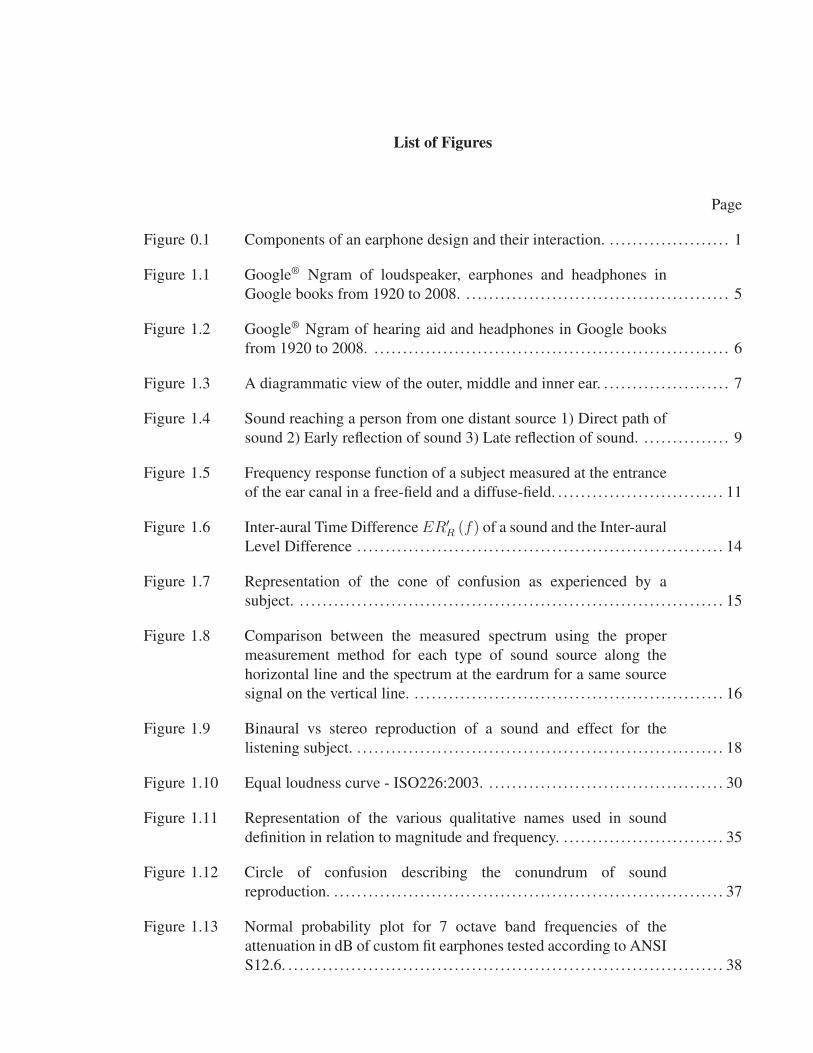
Figure 0.1 Components of an earphone design and
their interaction.

2
This thesis aims at identifying the contributing factors to a good sound signature as well as
the other components of earpiece design. All these components are interacting with each other,
as presented in Figure 0.1. Each topic can be analyzed on its own, but must also be analyzed
in conjuncture with the others to achieve a quality earpiece. Therefore, each of the contribut-
ing components to the earphone’s design is presented in a specific chapter and the relation to
the other components is explained. More specifically, this thesis explores the insert earphone,
which is defined as a "small earphone that fits either in the outer ear or is attached directly to a
connecting element, for example an earmould inserted into the ear canal" by the International
Electrotechnical Commission (2010a).
The diagram presented in Figure 0.1 was devised by cross-referencing publications made by
different authors in the last 60 years from several fields of study, including engineering and
psycho-acoustics. The main contributions of this thesis are to offer an extensive literature re-
view on earphone design and explore the coupling between the earphone and the ear, for which
future works is proposed in Chapter 4.
Chapter 1 explains the contributing factors that relate to the sound quality of an earphone.
It starts with an overview of the particularities of listening to a distant source versus with
earphones, covers the measurement of the sound quality of earphones and reviews the literature
to establish a definition of a target frequency response. The effect of the variability of each
factor is reviewed as well to determine their impact on the sound quality.
In Chapter 2, the measurement of earphones is explained. It includes the Frequency Response
Function (FRF), Total Harmonic Distortion (THD), Intermodulation Distortion (IMD), Multi-
Tone Distortion (MTD), and the triggered distortion, also called Rub and Buzz Distortion
(RBD). These are also metrics of the build quality of the earpiece because they are the direct re-
sults of the electroacoustic transduction process and the transformation of the acoustical power
by the geometry of the earphone and the ear canal. The electrical measurement, to determine
the main characteristics of transducers, including DC resistance and impedance measurement
in the small and large signal of the frequency domain are presented. The ear simulators and
measuring couplers necessary to measure the acoustical response are also shown in Chapter 2.
3
In Chapter 3, the modelling and simulation of the earphone are explained. Models of two
types of transducers typically used in earphone design are covered, namely the moving-coil
micro-loudspeakers and balanced-armature receivers. Models of acoustical components typi-
cally found in earphones design such as tubes, horns, meshes, generic cavities, etc. are also dis-
cussed in this chapter for various abstraction modelling methods: lumped-element, two-ports
(transmission line) and control-system block diagram.
Even if the frequency response function is considered as the foundation of sound quality in
earphones, at the time of publication no research has yet defined an unequivocal frequency re-
sponse as a "one size fits all". Even though many studies identify several factors that strongly
contribute to the pleasantness perceived by subjects, the challenge in finding a universal fre-
quency response comes from the variability in individual preference and in the physical shape
of the human ear. Therefore, there is a need for a customized process for the frequency response
is introduced in Chapter 4. This proposed process is intended to be usable across multiple smart
devices featuring increased signal processing capabilities. This suggestion is part of the future
works identified during this research that would contribute to a better understanding of the ear-
phone design such as new measurement tools and the perceptual effect of the coupling of the
earphone with the ear for a population.


Chapter 1
ACOUSTICS AND PSYCHO-ACOUSTICS OF EARPHONES
In the literature, when compared to loudspeakers, earphones represent a relatively new field
of study, which came lately with the rise of Portable Electronic Devices (PEDs). A Google ®
Ngram is a visual representation of the occurrence of a specific string within books indexed
by Google for a determined time frame. In Figure 1.1, it can be seen that the presence of
the word loudspeaker in books peaked in the mid-1950’s by being 6 times more prevalent
than earphones or headphones. The presence of the word headphones increased after 1965 and
surpassed loudspeaker in Google Books the years after the introduction of the iPod® by Apple®
in October 2001. Literally, the definition of the word headphones and earphones changed over
time, since over time both words were sometimes used to describe the same object. The word
headphones is becoming more prevalent in the literature while loudspeaker is disappearing.
Interestingly, loudspeaker design science is partially transferable to the earphone because of
a certain similarity in the application. However, the psycho-acoustics of loudspeakers are not
transferable as will be explored later in section 1.1.2.2. The word earphone will be used in
this thesis since it is defined by the International Electrotechnical Commission (2010a) as the
generic term for a device closely coupled acoustically to the ear.
Figure 1.1 Google® Ngram of loudspeaker, earphones and headphones in Google books
from 1920 to 2008. [English, Smoothing=1]
6
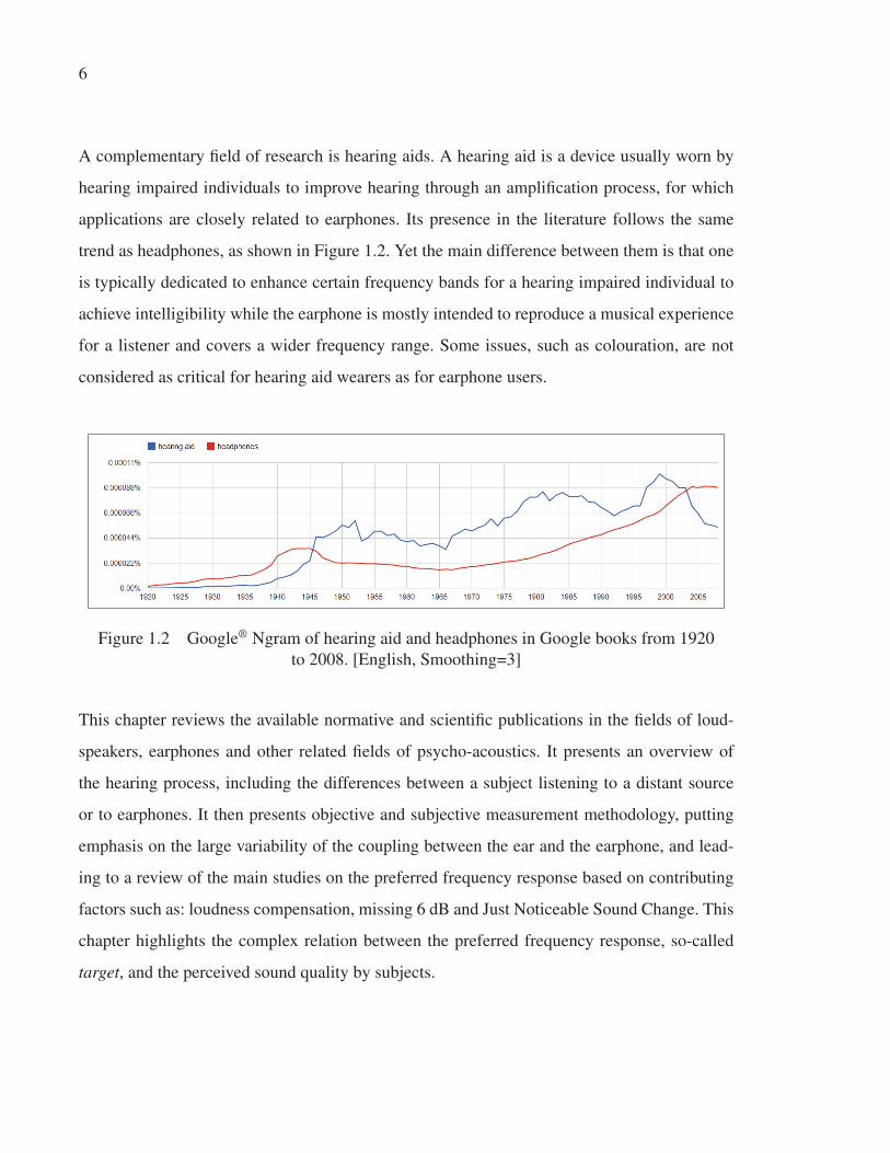
A complementary field of research is hearing aids. A hearing aid is a device usually worn by
hearing impaired individuals to improve hearing through an amplification process, for which
applications are closely related to earphones. Its presence in the literature follows the same
trend as headphones, as shown in Figure 1.2. Yet the main difference between them is that one
is typically dedicated to enhance certain frequency bands for a hearing impaired individual to
achieve intelligibility while the earphone is mostly intended to reproduce a musical experience
for a listener and covers a wider frequency range. Some issues, such as colouration, are not
considered as critical for hearing aid wearers as for earphone users.
Figure 1.2 Google® Ngram of hearing aid and headphones in Google books from 1920
to 2008. [English, Smoothing=3]
This chapter reviews the available normative and scientific publications in the fields of loud-
speakers, earphones and other related fields of psycho-acoustics. It presents an overview of
the hearing process, including the differences between a subject listening to a distant source
or to earphones. It then presents objective and subjective measurement methodology, putting
emphasis on the large variability of the coupling between the ear and the earphone, and lead-
ing to a review of the main studies on the preferred frequency response based on contributing
factors such as: loudness compensation, missing 6 dB and Just Noticeable Sound Change. This
chapter highlights the complex relation between the preferred frequency response, so-called
target, and the perceived sound quality by subjects.

7
1.1 Specificities of hearing sound emitted by a distant source versus with earphones
This section is not intended to be a comprehensive explanation of the human hearing process.
However, it would be useful to simply give a general notion of how sound waves into electrical
impulses that can be interpreted by the brain by describing the ear and the basic principles of
hearing from a distant source versus when wearing earphones.
1.1.1 Overview of the hearing process
Figure 1.3 A diagrammatic view of the outer, middle and inner
ear. [From "Tidens naturlære", Poul la Cour]
The human ear is divided into three sections, the outer ear, the middle ear and the inner ear.
A sectional view of the ear is presented in Figure 1.3. What is commonly called the ear -
part protruding the head - is scientifically known as the pinna (also known as the auricle).
The pinna collects and transforms incoming sound waves and redirects them into the ear canal
(or meatus), identified by (gg) in Figure 1.3. The sound waves then reach the eardrum, also
called tympanic membrane or tympanum (tf). The eardrum is the boundary between the outer

8
ear and the middle ear. It is important to note that this boundary is the limit of non-intrusive
physical measurement. As it will be explained in section 1.2.1, a measurement apparatus known
as a probe tube, can be used to measure sound pressure close to the eardrum. The outer ear’s
function is to collect a sound pressure and transfer this pressure to the eardrum. A sound source
close to the pinna or inserted into the ear canal, such as the use of earphones, would alter the
transfer function of the pinna. This is explored in section 1.1.2.2 and 1.1.3.
The middle ear, in a first approximation, is a mechanical system matching the impedance of
the sound in the outer ear, a gaseous medium, to the impedance of the fluid in the inner ear.
This impedance matching is possible due to the connection between the eardrum (tf) and the
oval window created by three bones - ossicles - called malleus (h), incus (a) and stapes (s). The
malleus (h) is connected to the eardrum while the stapes (s) is connected to the oval window.
The incus (a) relates the malleus (h) to the stapes (s) The oval window (not explicitly seen
in the Figure 1.3) is the interface between the middle ear and the cochlea (vh). Two major
components contributes to the impedance matching performed by the middle ear between the
outer ear and the inner ear. The first is the ratio of the surface area of the eardrum over the
oval window, matching the force by a surface variation. The second component contributing
to the impedance matching is the lever effect created by the ossicles. The displacement of the
malleus is slightly larger than the displacement of the stapes. This impedance matching leads
to the inner ear.
The inner ear could be seen as the spectrum analyser of the ear. It is a complex system per-
forming the conversion of the fluid pressure variations transmitted by the ossicles (h, a, s) into
an electrical signal. This conversion process is performed by a snail-shaped organ called the
cochlea (vh, vht, tht). Within this organ, a series of hairlike structures move with the fluid pres-
sure variations and activate nerves, which ultimately transmit the electrical signal through the
nervous system to the brain. Further explanation on how this process occurs can be found in
anatomy [Gelfand (2009)] and otolaryngology manuals [Nadol Jr. and McKenna (2005)].
9
1.1.2 Hearing a distant source: Sound paths, room reflections and the Head-Related
Transfer Function (HRTF)
When someone is hearing a sound, a complex interaction process between the sound source,
the environment and the human body transforms the sound wave before it reaches the tympanic
membrane. This interaction is explained in section 1.1.2.1, which explains the sound travelling
toward a subject. Then, section 1.1.2.2 explains how that sound is transformed by the contact
with the body until it reaches the tympanic membrane. These transformations are natural pro-
cesses of hearing and humans learn and adapt to these transformations. As a result they occur
almost subconsciously and need to be taken into account for an earphone design, as covered in
section 1.1.3.
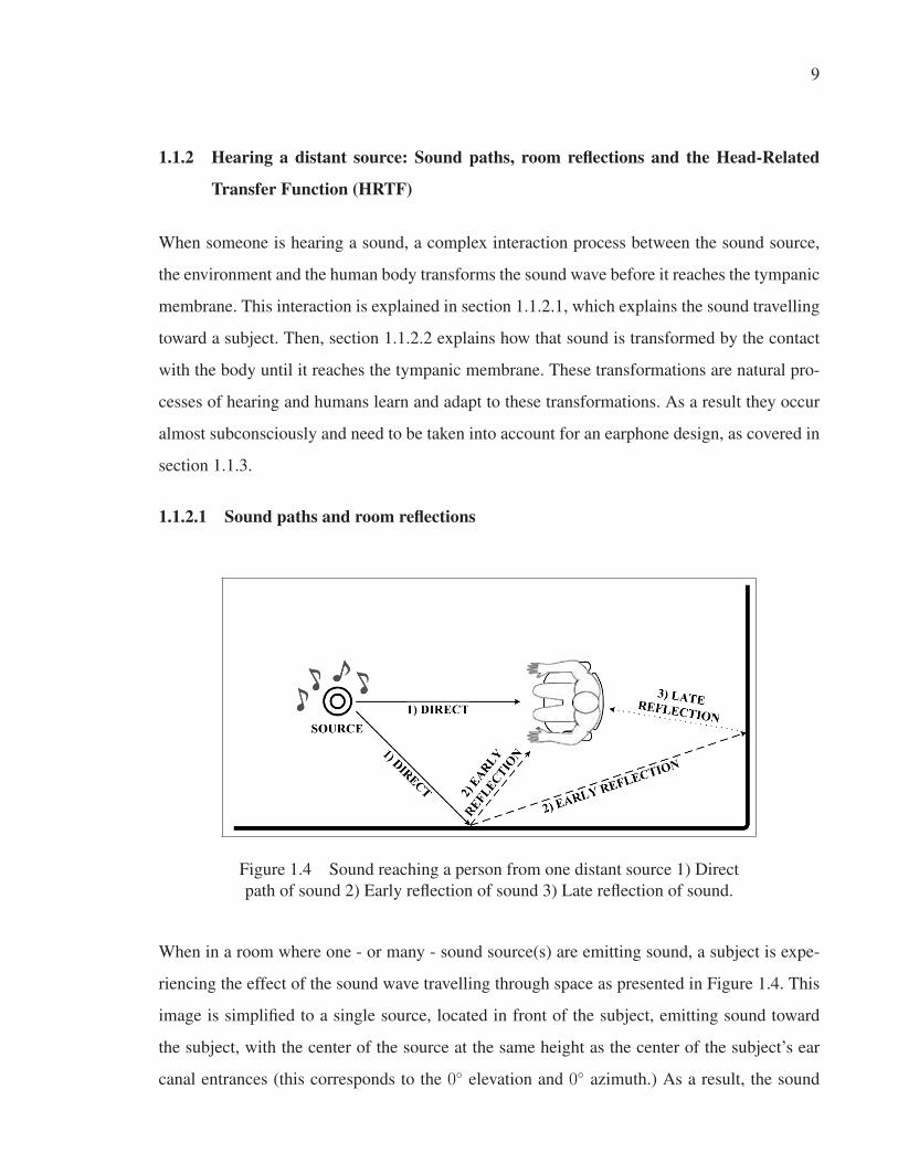
1.1.2.1 Sound paths and room reflections
Figure 1.4 Sound reaching a person from one distant source 1) Direct
path of sound 2) Early reflection of sound 3) Late reflection of sound.
When in a room where one - or many - sound source(s) are emitting sound, a subject is expe-
riencing the effect of the sound wave travelling through space as presented in Figure 1.4. This
image is simplified to a single source, located in front of the subject, emitting sound toward
the subject, with the center of the source at the same height as the center of the subject’s ear
canal entrances (this corresponds to the 0◦ elevation and 0◦ azimuth.) As a result, the sound
10
takes different paths to reach the pinna of the subject. Three of all possible paths are shown in
Figure 1.4 to demonstrate the combination of the direct and reverberant field. The first path to
reach the subject is the direct (1) path. The second path is the so-called early reflection (2) of
sound. The last sound to reach the subject is the so-called late reflection (3) of sound which
travels more distance before reaching the subject. The sound travelling by path 2 and 2+3 will
not reach the subject at the same time as the direct path since path 2 and 2+3 have a longer
distance to travel and the speed of sound (≈ 343 m/s) is constant. The difference between
an early reflection and a late reflection is the time it takes sound to travel to the measurement
point.
A room sound field can be quantified in relation to the reverberant field, or quantity of reflec-
tions compared to the direct sound. Beranek (1993) states that all the reflections reaching a
subject following the first 80 ms after the direct sound are part of the reverberant field. Oth-
erwise the early sound encompasses all the sound reaching the subject within the first 80 ms,
including the direct path of sound. From the definition established by Beranek (1993), it can be
seen that the two extreme fields are free-field equivalents and diffuse-field equivalents, defined
below:
• Free-field: The determination of the sound power level radiated in an anechoic or a hemi-
anechoic environment is based on the premise that the reverberant field is negligible at
the positions of measurement for the frequency range of interest.
• Diffuse field: At any position in the room, energy is incident from all directions with
equal intensities and random phases and the reverberant sound does not vary with the
receiver’s position.
As noted by Hodgson (1994), several factors such as surface reflection, surface-absorption
distribution and surface-absorption magnitude as well as fitting density are necessary to achieve
a diffuse field condition. Therefore, from the definition given above, a diffuse field is an ideal
reverberant field and if the required conditions are not met, the field is not diffuse.

11
1.1.2.2 Head Related Transfer Function
A Head-Related Transfer Function (HRTF) is a measurement of how a sound emitted from
a source located in a specific position in a three-dimensional space is modified, filtered and
shaped by the human body before it reaches a specific point of the ear canal(s) of a subject.
The most usual method to acquire a HRTF is by positioning a microphone or a probe tube at
the ear canal entrance and playing a sound from a loudspeaker positioned at a specific position
relative to the subject in a defined acoustic field environment. The HRTF defines the filters
required to process the signals sent to each ear in order to recreate the specified location of the
virtual sound source in space. This is later explained in this section. This binaural approach
gives the impression to the subject that a virtual sound source is located at the right position in
space.
103 104−5
0
5
10
15
20
Frequency (Hz)
Rel
ativ
e m
agni
tude
(dB
rel)
Free−Field (0° azimuth ,0°elevation)Diffuse Field Average
Figure 1.5 Frequency response function of a subject measured at the entrance of
the ear canal in a free-field and a diffuse-field.
The HRTF is dependant on two factors. The first, explained in section 1.1.2.1, summarizes how
the position of the sound source and its acoustic space influence the perception and measure-
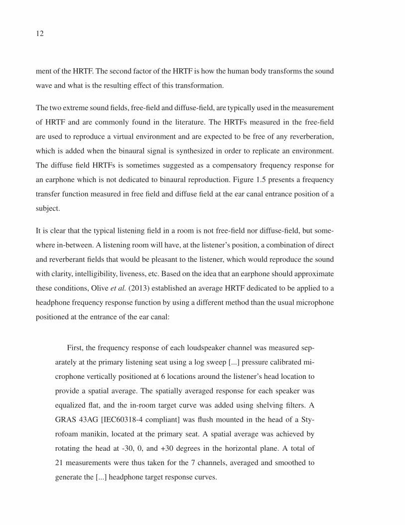
12
ment of the HRTF. The second factor of the HRTF is how the human body transforms the sound
wave and what is the resulting effect of this transformation.
The two extreme sound fields, free-field and diffuse-field, are typically used in the measurement
of HRTF and are commonly found in the literature. The HRTFs measured in the free-field
are used to reproduce a virtual environment and are expected to be free of any reverberation,
which is added when the binaural signal is synthesized in order to replicate an environment.
The diffuse field HRTFs is sometimes suggested as a compensatory frequency response for
an earphone which is not dedicated to binaural reproduction. Figure 1.5 presents a frequency
transfer function measured in free field and diffuse field at the ear canal entrance position of a
subject.
It is clear that the typical listening field in a room is not free-field nor diffuse-field, but some-
where in-between. A listening room will have, at the listener’s position, a combination of direct
and reverberant fields that would be pleasant to the listener, which would reproduce the sound
with clarity, intelligibility, liveness, etc. Based on the idea that an earphone should approximate
these conditions, Olive et al. (2013) established an average HRTF dedicated to be applied to a
headphone frequency response function by using a different method than the usual microphone
positioned at the entrance of the ear canal:
First, the frequency response of each loudspeaker channel was measured sep-
arately at the primary listening seat using a log sweep [...] pressure calibrated mi-
crophone vertically positioned at 6 locations around the listener’s head location to
provide a spatial average. The spatially averaged response for each speaker was
equalized flat, and the in-room target curve was added using shelving filters. A
GRAS 43AG [IEC60318-4 compliant] was flush mounted in the head of a Sty-
rofoam manikin, located at the primary seat. A spatial average was achieved by
rotating the head at -30, 0, and +30 degrees in the horizontal plane. A total of
21 measurements were thus taken for the 7 channels, averaged and smoothed to
generate the [...] headphone target response curves.

13
A shelf filter is reducing or enhancing, the frequencies under or above a transition frequency
of a desired gain while leaving the frequencies not included in the shelf at a unity gain.
The HRTF method used by Olive et al. (2013), that was developed and tested for circumaural
headphones, is expected to yield the best result as a predetermined frequency response for
earphones since it is based on a "preferred" listening field which is replicated for an average
person. However, the HRTF assumption as a basis for earphone is limited by the time invariant
nature of the earphone response because, for Schönstein and Katz (2010), "in order to achieve
high fidelity renderings many studies have shown that HRTFs need to be individualized for
the listener [...]" Schönstein and Katz (2010) explored the variability of the HRTF from a
perceptual point of view and concluded that any design solely based on a generic HRTF would
be affected by a large variability due to the subject’s morphology. Many studies were performed
to determine the variability of the HRTF and the contribution of each part of the human body
on the resulting HRTF: Mehrgardt and Mellert (1977), Hammershøi and Møller (1996), Hudde
and Schmidt (2009), Algazi et al. (2001) and Takemoto et al. (2012). From Algazi et al. (2001),
one can have an overview of the variability of the human anatomy, and therefore of the inter-
individual variations of the HRTFs.
Localization of sound is based on two phenomena, as presented in Figure 1.6. The first one
is when the sound reaches the subject and if the incident angle is not in quadrature with the
inter-aural axis, one of the sound path must travel further to reach the farther ear ERR (f) than
to reach the closer ear ERL (f). This phenomenon is the inter-aural time difference (ITD).
The second one is the sound level differences between a subject’s ears, because for frequencies
whose wavelengths are small relative to the dimensions of the head, the ear farther from the
source generally receives less energy than the nearer ear. This phenomenon is called inter-aural
level difference (ILD) - or inter-aural intensity difference (IID) - depending upon authors. In
Figure 1.6, this is represented by the change between ERR (f) and ER′R (f) linetype. The
change in the linetype represents the level variation compared to the original linetype after the
early reflection.

14
DR( f )DL( f )
ERR( f )
ERL( f )
ER' R(f )
Figure 1.6 Inter-aural Time Difference ER′R (f) of a
sound and the Inter-aural Level Difference (change in
linetype).
The previously mentioned ITD and ILD have a large impact on a subject’s perception of lo-
calization and space, the descriptor for localization and space will be covered in section 1.2.2.
Litovsky et al. (1999) explain: "the precedence effect [which] refers to a group of phenomena
that are thought to be involved in resolving competition for perception and localization between
a direct sound and a reflection. When the delay is zero and the speakers are stimulated equally,
the stimuli to the two ears of the listener are approximately equal and a single "fused" image
is perceived in the plane of symmetry, approximately straight ahead of the listener." Brown
and Stecker (2013) complete the idea by explaining that: "the precedence effect depends on
essentially two phenomena: (1) fusion of the early arriving (lead) and late-arriving (lag) sound
and (2) dominance of the localization cues carried by the lead over those carried by the lag
(termed localization dominance)". Again, Litovsky et al. (1999) note that there is a difference
depending on whether the sounds are presented in free field or over headphones. This effect
is of interest when music playback is intended since it is usually mastered with monitors and,
sometimes, evaluated over headphones after for comparison. The specificity of the ILD, ITD
evaluation with headphones will be discussed in section 1.1.3.
15
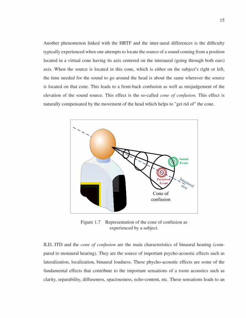
Another phenomenon linked with the HRTF and the inter-aural differences is the difficulty
typically experienced when one attempts to locate the source of a sound coming from a position
located in a virtual cone having its axis centered on the interaural (going through both ears)
axis. When the source is located in this cone, which is either on the subject’s right or left,
the time needed for the sound to go around the head is about the same wherever the source
is located on that cone. This leads to a front-back confusion as well as misjudgement of the
elevation of the sound source. This effect is the so-called cone of confusion. This effect is
naturally compensated by the movement of the head which helps to "get rid of" the cone.
Sound Event
Cone of confusion
Interauralaxis
Perceived Event
Figure 1.7 Representation of the cone of confusion as
experienced by a subject.
ILD, ITD and the cone of confusion are the main characteristics of binaural hearing (com-
pared to monaural hearing). They are the source of important psycho-acoustic effects such as
lateralization, localization, binaural loudness. These phycho-acoustic effects are some of the
fundamental effects that contribute to the important sensations of a room acoustics such as
clarity, separability, diffuseness, spaciousness, echo-content, etc. These sensations leads to an
16
impression of high-fidelity reproduction of a recording when proper - non-distorted - reproduc-
tion equipment is used. These criteria are discussed in section 1.2.
1.1.3 Hearing with earphones
FLAT LOUDSPEAKER
COLOUREDLOUDSPEAKER
FLAT EARPHONES
FIELD-CORRECTED EARPHONES
AT
THE
SOU
RCE
AT
EAR
DR
UM
PREFERED ACCEPTABLE POOR PREFERED
TYPE OF SOUND SOURCE
ME
ASU
RE
D S
PEC
TR
A
Figure 1.8 Comparison between the measured spectrum using the proper measurement
method for each type of sound source along the horizontal line and the spectrum at the
eardrum for a same source signal on the vertical line.
Figure 1.8 presents the frequency response for various types of electro-acoustic sound sources.
On the top horizontal lines, the source spectrum measured at the proper position in the proper
field is presented. On the bottom horizontal line, the frequency spectrum in the vicinity of the
eardrum is also presented for the proper measurement method. It can be seen that contrary to
sound coming form a distant source, sound produced by earphones do not involve the trans-
formation of the sound wave caused by the body as it naturally happens for a subject when a
distant source is used. A paradigm shift is necessary from what would be described as a flat
frequency response - the so-called X-curve for loudspeakers - for a distant source (first column)
to a corrected frequency response for an earphone which would recreate the distant field when
coupled with the ear (last column). Figure 1.8 also includes the effect of a coloured source,
meaning it is not a flat frequency response. When measured at the eardrum, it could be seen
as pleasing in certain situations by a group of subjects, as explained in section 1.2.2. An ear-

17
phone producing a flat frequency response is consider to have a poor perceived quality, when
Fleischmann et al. (2012) include this frequency response in perception evaluation of several
frequency responses.
Bauer (1961) established the foundation of stereophonic reproduction for earphones and bin-
aural loudspeakers and the basic principles underlying his work are still used and discussed
today. His statement explaining the effect: "this, evidently, is caused by the lack of suitable
cross-feed between the two ears", is still a valid statement from Atsushi and Martens (2006)
point of view:
This is primarily due to the effective absence of crosstalk between the two ears
signals delivered to the headphone user. In contrast, both loudspeaker reproduced
signals reach both of the listeners ears, and this crosstalk that occurs in loudspeaker
playback contributes significantly to the formation of stereophonic imagery. [...]
the resulting auditory spatial imagery is very different from the usual stereophonic
result, and has been termed biphonic to distinguish this result from the more fa-
miliar stereophonic imagery.
Consequently, most of the effort deployed since Bauer (1961) is to improve on his work and
make the integration between the stereophonic-intended recording and convert it into a quality
signal for earphones and not only a biphonic one. The principle of binaural reproduction and
stereo reproduction is presented in Figure 1.9.
The main challenge is that almost all music recordings are intended for stereophonic repro-
duction, so the earphone frequency response must be altered to take this fact into account, as
presented in Figure 1.8.
Litovsky et al. (1999) states that while the reproduction of a binaural environment over ear-
phones, as presented in Figure 1.8, "is successful in providing a quantitative measure of the
perceptual weights of the lead and lag, they certainly did not provide a realistic acoustic en-
vironment". Hartmann and Wittenberg (1996) investigated the use of simulated ITD and ILD
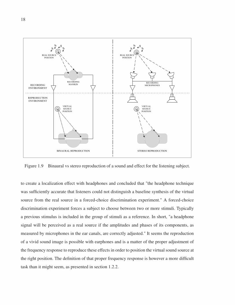
18
REPRODUCTION ENVIRONMENT
RECORDING ENVIRONMENT
BINAURAL REPRODUCTION STEREO REPRODUCTION
VIRTUAL SOURCE
POSITION
VIRTUAL SOURCE
POSITION
REAL SOURCEPOSITION
REAL SOURCEPOSITION
RECORDING MANIKIN
RECORDING MICROPHONES
Figure 1.9 Binaural vs stereo reproduction of a sound and effect for the listening subject.
to create a localization effect with headphones and concluded that "the headphone technique
was sufficiently accurate that listeners could not distinguish a baseline synthesis of the virtual
source from the real source in a forced-choice discrimination experiment." A forced-choice
discrimination experiment forces a subject to choose between two or more stimuli. Typically
a previous stimulus is included in the group of stimuli as a reference. In short, "a headphone
signal will be perceived as a real source if the amplitudes and phases of its components, as
measured by microphones in the ear canals, are correctly adjusted." It seems the reproduction
of a vivid sound image is possible with earphones and is a matter of the proper adjustment of
the frequency response to reproduce these effects in order to position the virtual sound source at
the right position. The definition of that proper frequency response is however a more difficult
task than it might seem, as presented in section 1.2.2.
19
Brown and Stecker (2013) reported that: "headphone stimuli that carry manipulated values of
one cue (e.g., ITD) but leave the other cue (ILD) fixed at zero are inherently artificial in that
they impose on a single stimulus substantial and consistent disagreement in the two major cues
to its location. While cues in the free field normally agree, being consistent in sign and ap-
proximately consistent in magnitude across azimuth, headphone stimuli introduce cue-conflict
and produce an unnatural perception of source location." Their analysis leads to the conclusion
that the fusion aspect of the precedence effect is more robust for stimuli lateralized by ITD
than stimuli lateralized by ILD. "This perceptual boundary between one fused sound and two
separate sounds is often referred to as the echo threshold." The binaural effect expected from
a distant source and reproduced over earphones are still under investigation and still open to
argument over its quality.
1.1.4 Coupling of the earphone with the ear
From an electro-mechanic point of view, in a first approximation, a distant sound source is
typically impeded by a coupling impedance corresponding to free air (Z = ρc) which is often
approximated to 415± 10[
Pa·sm
]for an operating temperature of 20± 12◦C. This would result
in a variation of 0.2 to 2 dB. Ciric and Hammershøi (2006) reported that the coupling between
the earphone and the ear is critical:
The acoustic loading of the pinna, ear canal, eardrum, and ossicular chain are
potential sources that influence the acoustic signal received by the eardrum. [...]
Two distinct factors are related to the variability [of the frequency response]; A
factor causing the variability at low frequencies, and resulting in uncontrolled
variations of the pressure, is the leakage. [...] at higher frequencies (above ap-
proximately 2000 Hz), the sound pressure depends on the wave properties of the
earphone and the external ear. In this frequency region, the size and shape of the
cavity enclosed by the earphone, factors that are dependent on the earphone and its
positioning, the geometry of the pinna, and the ear canal, become very important.

20
The calculation of the variation of the coupling between the earphone and the ear which "de-
pends on individual subject characteristics and on the earphone itself" is a process presented by
Møller et al. (1995a), as discussed in section 1.2.1. Using this method, Ciric and Hammershøi
(2006) found larger standard deviations, compared to a measurement with a coupler defined in
section 2.2, in the low and mid frequencies (5 to 8 dB) when supra-aural earphones are used
compared to circumaural ones (2 to 3 dB). The earphone types are defined by the International
Electrotechnical Commission (2010a). Ciric and Hammershøi (2006) concluded that a large
impedance variation "in the order of 15 dB or even more" is to be expected for the frequency
response of an earphone, which is much larger than what is expected in a free field, as they
measured. For headphones, the impact of the pinna is to be considered. "At higher frequencies
(above approximately 2000 Hz), the sound pressure depends on the wave properties of the ear-
phone and the external ear. In this frequency region, the size and shape of the cavity enclosed
by the earphone, factors that are dependent on the earphone and its positioning, the geometry
of the pinna, and the ear canal, become very important."
In principle, for insert earphones, the pinna is not accounted for as an impedance load, as just
stated. However, Oksanen et al. (2012) did study the individual sound pressure levels at the
eardrum for insert earphones and reported that: "deviations of approximately 3 mm from the
average diameter of the ear canal could cause errors above 3 dB [...] However, deviations that
large were not seen amongst the test participants [of their study]." In the same line of thought,
Valente et al. (1994) measured the SPL near the eardrum for six discrete frequencies between
500 and 4000 Hz using conventional (TDH-39P) and insert earphones (ER-3A), the magnitude
of the intersubject variability determined and concluded that "the presence of large intersubject
differences in the SPL measured near the eardrum questions the validity of predicting individ-
ual performance based upon averaged group data. Intersubject differences were independent of
the type of earphone used to make the measure."
From an earphone design point of view, this variation is important because two people can have
a different perception of the sound quality solely because the coupling to the ear changes the
SPL at the eardrum and not because the subject would not appreciate the response for which
21
the earphone is designed for. Furthermore, another observation by Valente et al. (1994) is that
the type of earphones have a significant impact on the SPL measured at the eardrum for a same
subject. Again, this might have an impact on the perceived quality. Sound signature evaluation
is explained in section 1.2 which explains the measurement of the sound quality of earphone
and the contributing factors to this perceived quality while section 1.3 explores important study
on the relation between the measured frequency response and the perceived sound quality of
earphone.
1.2 Measuring the sound quality of earphones
As briefly presented in the previous section, measuring the sound quality of an earphone is per-
formed by measuring objective metrics but also subjective metrics to understand how subjects
perceive an acoustical phenomenon. This section presents the main methods used to assess the
sound quality of an earphone. Electro-acoustic engineers design products that will ultimately
be used on or by humans. On the one hand, to assess sound quality, objective measurements us-
ing measurement tools that are fitted in the ear or a replicate human’s outer-ear are performed
and objective metrics are recorded, as described in Chapter 2. On the other hand, subjective
measurements obviously require the an active participation of the subject. The validity of the
measurement depends on the input from the subject. Some measurement methods, like a probe
tube inserted into a subject’s ear canal, are used to compare the subject’s perception with the
physical measurement. This relationship between the subjective and objective measurements is
known as the Perceptual Evaluation of Audio Quality (PEAQ). As it will be presented in sec-
tion 2.2, the ITU-T recommendation has been modified by Temme et al. (2012) for loudspeaker
and headphones applications.
1.2.1 Objective measurement of sound quality
Two methods are used to perform objective measurement of sound quality: the Acoustic Test
Fixture (ATF) and the probe microphone. By using either of these measurement methods, the
ATF or the probe microphone, it is possible to compare the perceptual effect elicited by a
subject to an "absolute" physical reference.

22
1.2.1.1 Acoustic test fixture
The so-called Acoustic Test Fixture (ATF) is a simulator that enables objective measurement
of sound. A type of ATF is the Head and Torso Simulator (HATS), as normalized by the Inter-
national Electrotechnical Commission (2011). It is intended to simulate the change that occurs
to sound waves as they pass a human head and torso, the HRTF defined in section 1.1.2.2. It
is fitted with a rubber-like replica (called pinna simulator) of an average ear with a fixture that
includes a microphone to replace the ear canal and eardrum. Toole (1984) readily noted that
"the rubber replica was mechanically different from a real external ear and it did not fold and
crush as readily in the same manner as the real thing". This lack of mechanical properties repli-
cation discourages any attempt to have an earphone that modifies the shape of the ear such as a
supra-aural type since the pinna simulator is still mono-material and does not behave as a real
ear would, with its complex blend of hard cartilage and softer tissue. A proper ear simulator
for these types would be made of several layers of various material properties to simulate the
movement of the cartilage and skin.
Measurement of supra-aural and circumaural earphones is performed using the coupler spec-
ified by the International Electrotechnical Commission (2009). The details of these couplers
are explained in section 2.1. Inanaga et al. (2008) and Hiipakka et al. (2010) investigate the
intra-aural and insert earphones and Blau et al. (2010) the variability between the coupler and
real ears. Blau et al. (2010) concluded that "the less frequently used artificial ears do a better
job in representing the average ear, but can of course not account for interindividual differences
in ear canal acoustics, which may reach 20 dB in the frequency range up to l0 kHz."
1.2.1.2 Probe microphone
An alternative to the use of ATF is the use of a very small microphone, also called probe mi-
crophone tube, at the entrance, or inserted into the ear canal, which records the sound pressure
transformed by the pinna and the ear canal and measures how the sound is affected by the
outer ear, as explained in section 1.1.2.2. This method also presents limitations, mostly due to
23
disturbance in the wave propagation in the ear canal but is used because it is a viable way to
assess inter-subject variation.
The validity of the method for circumaural earphones has been explored by Møller et al. (1992,
1995a,b). They found an intra- and inter-subject variability which is qualified as: "in general
the error is low up to 7 kHz. Above this frequency the error increases to an almost constant
level for the rest of the audio frequency range. [...] The blocked ear canal method provides the
smallest standard error of the mean. The reason is that the method totally ignores the effect of
the ear canal [...]".
Unfortunately, the blocked ear canal is not very useful for the measurements of intra-aural and
insert earphones. However, Blau et al. (2010) stated that "probe tube measurements [...] become
inaccurate at high frequencies (above a few kHz) if the probe tube is not positioned in the
immediate vicinity of the ear drum, which is difficult to assure in everyday practice. In occluded
ear situations (e.g., closed ear molds for hearing aids), probe tube measurements suffer from
leaks caused by the presence of the tube, resulting in large errors at low frequencies (typically
below 1 kHz)." The probe microphone tube measurement made by Ciric and Hammershøi
(2006) also lead them to several conclusions related to the use of probe microphones:
• For frequencies under 1 kHz, an earphone could be considered as a nearly ideal sound
pressure source;
• The Thévenin impedances for free-field and earphone exposure (the radiation and ear-
phone impedance) are considerably smaller than the impedance of the ear canal at low
frequencies;
• The intrasubject and intersubject variations of the earphone transfer functions [between
the voltage and the SPL] confirm that the sound pressure level generated in an ear could
differ considerably from the defined value. This difference could be in the order of 15 dB
or even more;
• The earphone transfer functions measured in human ears differ from the corresponding
ones measured in the coupler, especially when individual functions are analysed;
24
• All earphones could be considered to behave very similar on a mean basis in respect to
the ratio of the earphone impedance and the impedance of the average human ear canal;
• Some important effects of coupling of [...] earphones to human ears do not exist in cou-
pling of the earphones to the coupler.
1.2.2 Subjective measurement of sound quality
Perceptual audio evaluation of a product is a murky topic summarized by Bech and Zacharov
(2006) who describe methodologies and list the bounds of perceptual audio evaluations. They
cover the important components of a study, namely the definition of test, experimental vari-
ables, calibration, reproduction equipments and rooms, quantification of impressions and statis-
tics. Bech and Zacharov (2006) explain the challenge related to the subjective measurement of
sound quality:
[Subjective measurement of sound quality is] focused on a specific attribute
of the sound, and often the stimuli are specifically designed to (hopefully) excite
the attribute of interest. This often has the consequence that the stimuli are (very)
synthetic and thus quite dissimilar to the natural sounds. [...] The starting point is
the existence of an acoustically complex stimulus a sound field impinging on the
ears of a subject which is then transformed by the physiology and neurology of
the hearing system into neural energy. The acoustic stimulus is characterized by
physical measurements of variables [...].
Elicitation is defined by Merriam-Webster (1998) as "the process by which something latent
or potential is brought out". Again, Bech and Zacharov (2006, p.43-44) indicate that direct
elicitation method assume "there is a close relationship between a given sensation and the
verbal descriptors used by the subject to describe the sensation." Indirect elicitation "tries to
separate sensation and verbalisation, as verbalisation, it is argued, depends strongly on the size
and availability of suitable terms in the subject’s lexicon." Secondly, it is questioned whether
the assumed relationship between what is being said and what is being perceived actually exists

25
while non-verbal elicitation is described as "the information communicated from one person
to another in addition to the verbal communication. This includes hands and arm movements
such as when the person points in a given direction to indicate the origin of the sound or when
the explanation of something is accompanied by a sketch, and so on."
The foundation of comparative judgement, often used in audio quality perception comes from
Thurstone (1927) who describes how to compare the physical stimulus intensities and also
the qualitative comparative judgement like for the excellence of specimen. Most of the work
relative on judgement is still based on the principles he established. For example, Letowski
(1989) categorized auditory judgements as:
A formalized auditory assessment may be of heuristic or diagnostic character.
In the former case, the purpose of assessment is to collect normative data while in
the latter case the purpose is to evaluate if and to what extend a specific property
or an object differs from the accepted standard. The aim of such auditory assess-
ment is either to gather information about the external world (objects) or about the
listeners themselves (subjects).
These two dichotomies create four basic domains of auditory judgements as shown in Table
1.1.
Table 1.1 Basic applications of auditory assessment
Subject-oriented tests Object-oriented testsHeuristic judgements Psychoacoustic Research Sound Quality Assessment
Diagnostic judgements Audiological Evaluation Diagnostic Listening Tests
Letowski (1989) also identifies three criteria for the subjective evaluation of sound quality:

26
• Fidelity (accuracy): relates one auditory image to another, like a standard or a golden
reference. It is a way to quantify any modifications that may occur to a signal between
the input and the output of a device;
• Naturalness: relates an auditory image to a specific internal standard, which can be a
generalized conceptual image residing in the memory of the listener and used as the
point of reference;
• Pleasantness: relates an auditory image to a set of various internal standards, manifesta-
tion of the subjective satisfaction resulting from listening to a given sound.
Letowski (1989) notes that "there are situations (synthetic signals, hearing impaired listeners,
etc.) where less natural sounds can be regarded as more pleasing." Bech and Zacharov (2006)
agree that an unnatural sound may elicit more pleasantness than a natural sound of the same
nature, like in music. Gabrielsson et al. (1990) completes the idea: "Overall evaluations of the
systems in terms of fidelity of pleasantness may be regarded as weighted combinations of the
separate perceptual dimensions. [...] Among the physical variables the frequency response is
often considered as the most important." They explain the perceptual dimension:
Brightness and sharpness increase (dullness and softness/gentleness decrease)
with rising frequency response toward higher frequencies and/or falling response
toward higher frequencies and/or falling response toward lower frequencies. [...]
Fullness is favoured by a broad frequency range and relatively more emphasis on
lower frequencies. [...] Clarity, spaciousness, and (to some extent) nearness are
likewise favoured by a broad frequency range, often with a certain emphasis on
midhigh to high frequencies.
In addition, Lorho (2005) divided necessary attributes for the audio evaluation of headphones
into three (3) dimensions, namely: localization, space and timbre. Attributes related to distance,
direction, movement and localization are presented in Table 1.3. These attributes are related to
a common criticism made about earphones: the sound is within the head, not solid in front of
the subject, as stereo provides which is an attribute of localization.
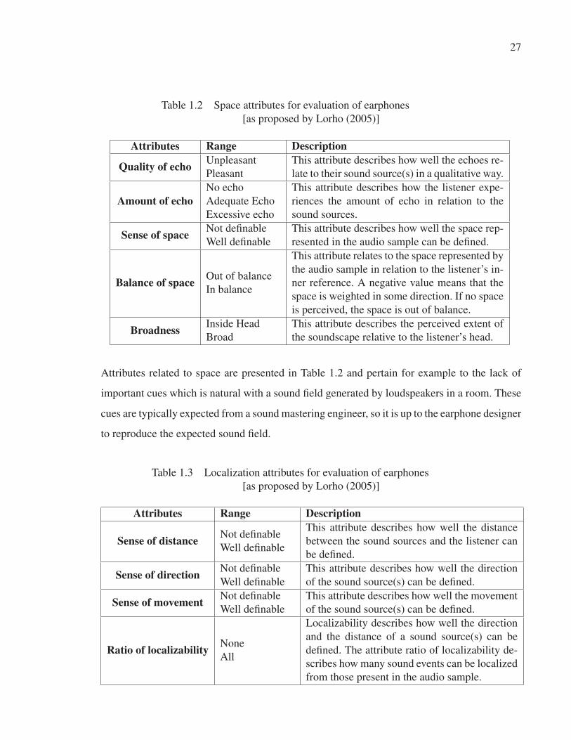
27
Table 1.2 Space attributes for evaluation of earphones
[as proposed by Lorho (2005)]
Attributes Range Description
Quality of echo Unpleasant
Pleasant
This attribute describes how well the echoes re-
late to their sound source(s) in a qualitative way.
Amount of echoNo echo
Adequate Echo
Excessive echo
This attribute describes how the listener expe-
riences the amount of echo in relation to the
sound sources.
Sense of space Not definable
Well definable
This attribute describes how well the space rep-
resented in the audio sample can be defined.
Balance of space Out of balance
In balance
This attribute relates to the space represented by
the audio sample in relation to the listener’s in-
ner reference. A negative value means that the
space is weighted in some direction. If no space
is perceived, the space is out of balance.
Broadness Inside Head
Broad
This attribute describes the perceived extent of
the soundscape relative to the listener’s head.
Attributes related to space are presented in Table 1.2 and pertain for example to the lack of
important cues which is natural with a sound field generated by loudspeakers in a room. These
cues are typically expected from a sound mastering engineer, so it is up to the earphone designer
to reproduce the expected sound field.
Table 1.3 Localization attributes for evaluation of earphones
[as proposed by Lorho (2005)]
Attributes Range Description
Sense of distance Not definable
Well definable
This attribute describes how well the distance
between the sound sources and the listener can
be defined.
Sense of direction Not definable
Well definable
This attribute describes how well the direction
of the sound source(s) can be defined.
Sense of movement Not definable
Well definable
This attribute describes how well the movement
of the sound source(s) can be defined.
Ratio of localizability None
All
Localizability describes how well the direction
and the distance of a sound source(s) can be
defined. The attribute ratio of localizability de-
scribes how many sound events can be localized
from those present in the audio sample.

28
Attributes related to timbre, which are most frequently used when there is a need to describe
how earphones sound, are presented in Table 1.4
Table 1.4 Timbre attributes for evaluation of earphones
[as proposed by Lorho (2005)]
Attributes Range Description
Separability None
All
This attribute describes how well the sound
events can be [singled] out in the audio sample.
Tone color
Lower sounds
emphasized
Higher sounds
emphasized
This attribute describes the spectral content of
the audio sample.
RichnessFlat
Neutral
Rich
This attribute describes how rich and nuanced
the audio sample is overall, and relates to a
combination of harmonics and dynamics per-
ceived in the sample.
Distortion Distorted
Not distorted
This attribute describes the possible metallic,
machine-like, electrical-like artifacts in the au-
dio sample.
Disruption Disrupted
Not disrupted
This attribute describes how much hiss,
snap/crackle/pop is perceived in the audio sam-
ple.
Clarity Muffled
Clear
This attribute describes if the sound sample ap-
pears clear of muffled, for example if the sound
source is perceived as covered by something.
Balance of Sounds Out of balance
Well balanced
This attribute describes the possible difference
in loudness between the sound sources present
in the audio sample. The sound sample is well
balanced if it contains only one sound source.
The attributes presented in the Tables 1.2, 1.3 and 1.4 define one dimension of sound quality
at a time, the complex interrelation between each has to be assessed from a general, overall,
impression. In practice, every researcher establishes his own test protocol in order to elicit the
studied attributes as reported by Bech and Zacharov (2006). However, as explained by Borwick
et al. (2001, p.565-584), the testing protocol should limit the presence of nuisance factors. Nui-
sance factors may be of a bias nature or of external nature. A typical testing approach would
invite one, or many subject(s) to sit in a room where listening equipment is already installed.

29
If the researcher wants to know the impact of the colour, shape or size of the device under test
(DUT) on the perceived quality, the subject will be allowed to see the DUT and - hopefully
- change his perception because of that, otherwise, the DUT will be hidden from the subject.
Then specific stimuli will be played and the subject will be asked to comment on the studied
attributes, either verbally of by way of a standard evaluation form. In this case, affective mea-
surement is of high interest. Bech and Zacharov (2006, p.65-67) explain in detail the affective
measurement: Preference tests, Acceptance tests and Appropriateness tests. For these tests, the
scales and statistical processing are described by the authors. The studies presented in the later
sections are essentially based on these tests, which although somewhat different rely on the
same process of elicitation and description of a phenomenon.
1.2.3 Loudness and earphone sound quality
As explained by Toole (2008, p.432), "loudness is the perceptual correlate of sound level. It is
dependent on frequency, sound level, incident angle, the duration of the signal, and its tempo-
ral envelope." The subjective judgement of the loudness amplitude level of a sound referenced
in SPL is expressed in phons. The phon is numerically equal to the median sound pressure
level in decibels of a 1000-Hz reference tone. This difference exists to demonstrate the sub-
jective aspect of the measurement. The normalized equal loudness curves are compiled in the
International Organization for Standardization (2004) (ISO226:2003). Equal loudness is de-
fined as an intensity sensation divided in two types of loudness models, the time-variant and
time-invariant models. By definition, the time-variant models should be processed using active
methods, beyond the scope of this work, which use a signal processor to analyse the sound sig-
nal and apply loudness corrections accordingly. The proper loudness compensation is expected
to have an important impact on the perceived quality, since it is an indicator of richness and
other descriptors of audio quality, as presented in Figure 1.11. In Figure 1.11, various descrip-
tors of the perception of sound are related to the relative variation of amplitude for a range of
frequency. For example, in the low end of the spectrum, a positive gain in amplitude is related
to a perception of solidity. Gabrielsson et al. (1990) noted that "The available evidence indi-
cates that an increase in sound level will usually increase the perceived fullness, spaciousness,
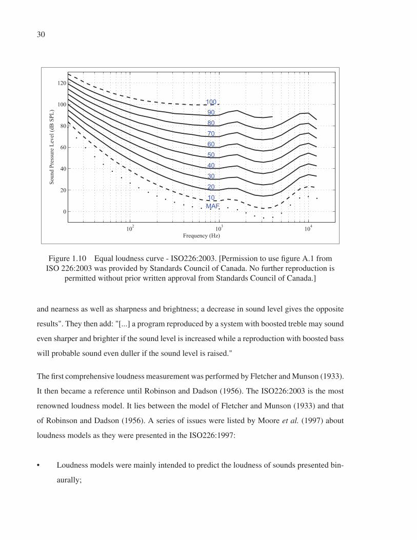
30
102 103 104
0
20
40
60
80
100
120
Frequency (Hz)
Soun
d Pr
essu
re L
evel
(dB
SPL
)
MAF10
2030
405060708090100
Figure 1.10 Equal loudness curve - ISO226:2003. [Permission to use figure A.1 from
ISO 226:2003 was provided by Standards Council of Canada. No further reproduction is
permitted without prior written approval from Standards Council of Canada.]
and nearness as well as sharpness and brightness; a decrease in sound level gives the opposite
results". They then add: "[...] a program reproduced by a system with boosted treble may sound
even sharper and brighter if the sound level is increased while a reproduction with boosted bass
will probable sound even duller if the sound level is raised."
The first comprehensive loudness measurement was performed by Fletcher and Munson (1933).
It then became a reference until Robinson and Dadson (1956). The ISO226:2003 is the most
renowned loudness model. It lies between the model of Fletcher and Munson (1933) and that
of Robinson and Dadson (1956). A series of issues were listed by Moore et al. (1997) about
loudness models as they were presented in the ISO226:1997:
• Loudness models were mainly intended to predict the loudness of sounds presented bin-
aurally;
31
• The ISO226:1997 did not correctly predict the relationship between monaural loudness
and binaural loudness;
• Contours are significantly affected by biases [such as sound transmission path in the low
frequencies];
• The models predict zero loudness (MAF in Figure 1.10) for the absolute threshold even
if the absolute threshold is statistically determined [by a method of average, standard
deviation of subjects threshold].
A definition of bias is given in 1.3.2. Moore et al. (1997) propose a new time-invariant loudness
model based on earphone measurements to limit the biases. In the International Organization
for Standardization (2004), these concerns were not addressed and since this standard is for
ontologically normal people aged between 18 and 25 inclusively, it has a limited application
for earphone development on a mass-consumer scale. Defining the best model to compensate
for loudness for earphones is yet to be presented, but the inclusion of a loudness model in
the frequency response seems to show more advantages than drawbacks. This is because most
earphone users are not in a fixed environment and the ambient noise changes, so the users
change the SPL of the earphone in order to keep a proper signal-to-noise ratio, as later presented
in section 1.2.4.1.Variations in SPL have an impact on perceived loudness and should be taken
into account.
1.2.3.1 Just-Noticeable Sound Changes
Just-Noticeable Sound Changes (JNSC) are the minimum variation of amplitude of a given
stimulus that can be perceived by a subject. As explained by Zwicker and Fastl (2007, p.175),
two types of assessments are possible for a variation of sound change. The just-noticeable
variation is a level of comparison which is used to adjust one source to match a known quality
reference source for a psychological attribute. Signal matching of a test apparatus to a reference
source is used for earphone design for loudness balancing. Bech and Zacharov (2006) explain
loudness balancing for headphones:
32
Loudness balancing aims to match the level of headphone reproduction to that
of a source (e.g. loudspeaker) in a given sound field. The sound field often com-
prises either a free field or a diffuse field. Subjects listen to one-third octave, band-
pass filtered pink noise from the loudspeaker source and then over headphones.
The subjects then adjust the level of the headphone to match the loudspeaker’s
level using the method of adjustment. This process is iterated until the subjects
find the matching loudness level in each frequency band. Typically, eight subjects
are used for this process. Such methods are defined in detail in IEC 60268-7 and
have applications in both diffuse and free-field measurements [See section 2.2.1
for complementary information].
The other option is the comparison of differences, the just noticeable difference, between two
similar objects which are in essence the same but show differences that can be described by
a subject. This assessment depends on several factors. Is the assessment of monaural (1 ear)
or of binaural (both ears) nature? Is the type of stimuli used of a nature that would allow
the proper elicitation for which the test was designed for? These two Just-Noticeable Sound
Changes methods are used to test earphones, the matching of signal between a reference source
and the earphone is the most commonly used approach. The variation as a function of time
is used principally to explain the perceived quality of the same signal on the same listening
apparatus when one of the components is changed. The other aspect is related to the quality
of the design. The JNSC can be analysed in frequency, amplitude, phase, etc. The JNSC in
loudness is explored in section 1.2.3.2. The JNSC in frequency is mentioned in section 2.2.3.
1.2.3.2 Signal matching and loudness function
From an earphone designer’s point of view, loudness has specificities related to the character-
istics of reproduction, recording and mastering method used. Morgan and Dirks (1974) studied
the loudness discomfort levels (LDL) and the alternate binaural loudness balance (ABLB) for
earphones compared to a free-field equivalent. They concluded that "when the sound pressure
level in the ear canal under earphone or in the free field is accounted for, there are essentially no
differences between the two measuring conditions for suprathreshold loudness measures." It is
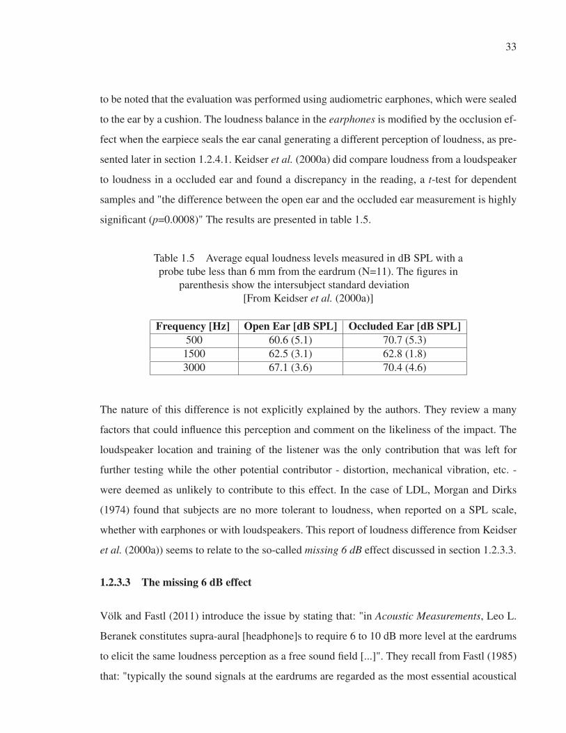
33
to be noted that the evaluation was performed using audiometric earphones, which were sealed
to the ear by a cushion. The loudness balance in the earphones is modified by the occlusion ef-
fect when the earpiece seals the ear canal generating a different perception of loudness, as pre-
sented later in section 1.2.4.1. Keidser et al. (2000a) did compare loudness from a loudspeaker
to loudness in a occluded ear and found a discrepancy in the reading, a t-test for dependent
samples and "the difference between the open ear and the occluded ear measurement is highly
significant (p=0.0008)" The results are presented in table 1.5.
Table 1.5 Average equal loudness levels measured in dB SPL with a
probe tube less than 6 mm from the eardrum (N=11). The figures in
parenthesis show the intersubject standard deviation
[From Keidser et al. (2000a)]
Frequency [Hz] Open Ear [dB SPL] Occluded Ear [dB SPL]500 60.6 (5.1) 70.7 (5.3)
1500 62.5 (3.1) 62.8 (1.8)
3000 67.1 (3.6) 70.4 (4.6)
The nature of this difference is not explicitly explained by the authors. They review a many
factors that could influence this perception and comment on the likeliness of the impact. The
loudspeaker location and training of the listener was the only contribution that was left for
further testing while the other potential contributor - distortion, mechanical vibration, etc. -
were deemed as unlikely to contribute to this effect. In the case of LDL, Morgan and Dirks
(1974) found that subjects are no more tolerant to loudness, when reported on a SPL scale,
whether with earphones or with loudspeakers. This report of loudness difference from Keidser
et al. (2000a)) seems to relate to the so-called missing 6 dB effect discussed in section 1.2.3.3.
1.2.3.3 The missing 6 dB effect
Völk and Fastl (2011) introduce the issue by stating that: "in Acoustic Measurements, Leo L.
Beranek constitutes supra-aural [headphone]s to require 6 to 10 dB more level at the eardrums
to elicit the same loudness perception as a free sound field [...]". They recall from Fastl (1985)
that: "typically the sound signals at the eardrums are regarded as the most essential acoustical

34
input parameters leading to auditory sensations in subjects." The 6 dB difference at minimum
audible pressure (MAP) between a loudspeaker source and an earphone is attributed to method-
ological shortcomings, as identified by Killion (1978). However, as presented above, the study
by Keidser et al. (2000b) identified a similar effect for insert earphones in levels above the
minimum audible pressure (MAP), interestingly the difference is 10 dB, as noted by Beranek.
Völk and Fastl (2011) explain that "different inter-aural phase relations are not detected by
the sound level" and when explored from a binaural perception point of view, "comparing the
situations with the same (root-mean-square) sound pressure levels caused by headphone and
loudspeaker box reproduction does not assure the same ear signals. [Because] identical time
functions of the ear signals in headphone and loudspeaker reproduction on the contrary actually
leads to equal loudness perception at equal level in the auditory canal." Their conclusion is that
the same loudness perception can only be elicited if the auditory event position is comparable
in both cases.
1.2.3.4 Identifying the reference recording SPL to differentiate the proper loudness
transfer function
In Figure 1.11, an interesting representation of the complexity of managing loudness in sound
reproduction is presented by Alten (2011). Perceptual evaluation of the audio quality is a com-
pound of many of these features and the attempt to dissociate (elicit) each of them individually
to explain their impact on the overall experience proves to be a challenge in itself because it
implies that the recording and restitution chain are fully controlled.
Unfortunately, no recording explicitly states the recording level at which the original sound
was recorded nor the recording equipment that was used, making it difficult to evaluate the
right listening level at which a reproduction equipment could be evaluated. Furthermore, the
equipment used to do the recording in the first place has been evaluated by using recordings
at an unknown SPL with equipment of unknown quality. This conundrum, identified by Toole
(2008), is presented in figure 1.12. Gabrielsson et al. (1974) noted this fact in their experiment
: "This may partly be explained by the reference to the sound level and the frequency range of
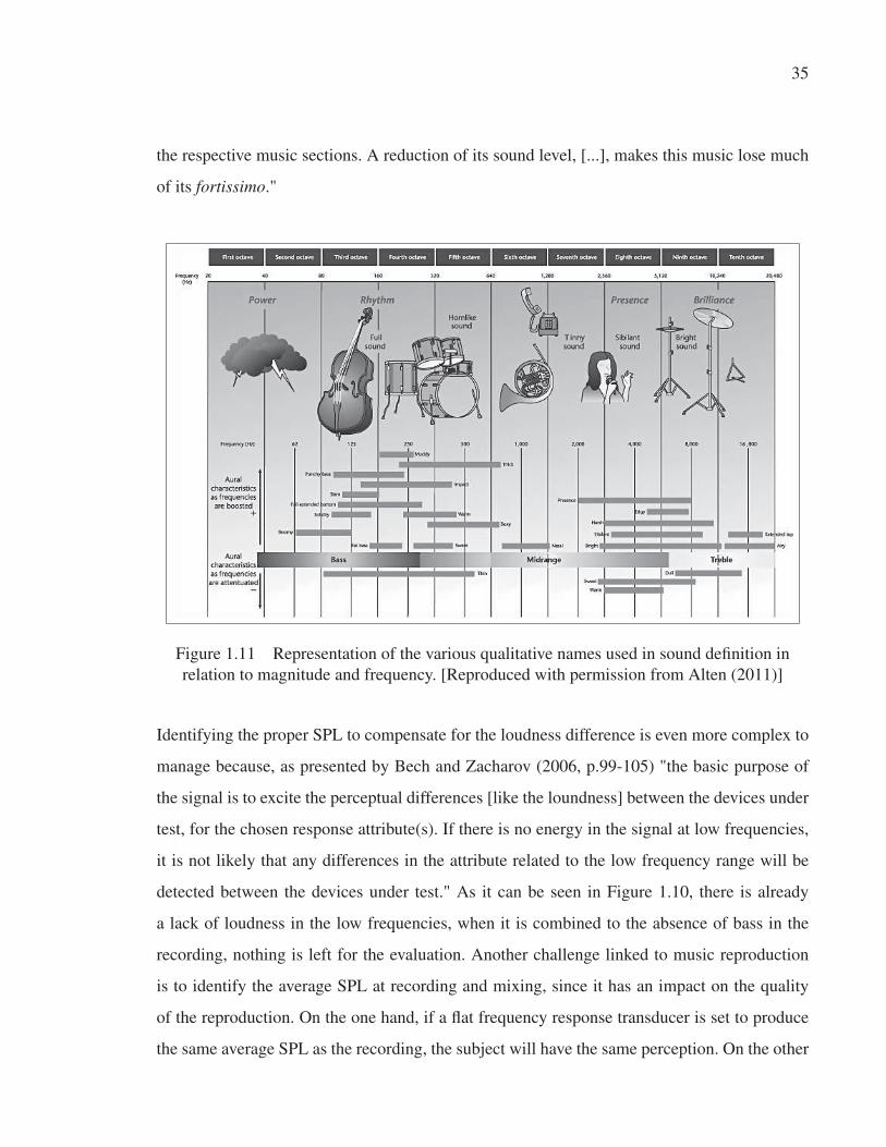
35
the respective music sections. A reduction of its sound level, [...], makes this music lose much
of its fortissimo."
Figure 1.11 Representation of the various qualitative names used in sound definition in
relation to magnitude and frequency. [Reproduced with permission from Alten (2011)]
Identifying the proper SPL to compensate for the loudness difference is even more complex to
manage because, as presented by Bech and Zacharov (2006, p.99-105) "the basic purpose of
the signal is to excite the perceptual differences [like the loundness] between the devices under
test, for the chosen response attribute(s). If there is no energy in the signal at low frequencies,
it is not likely that any differences in the attribute related to the low frequency range will be
detected between the devices under test." As it can be seen in Figure 1.10, there is already
a lack of loudness in the low frequencies, when it is combined to the absence of bass in the
recording, nothing is left for the evaluation. Another challenge linked to music reproduction
is to identify the average SPL at recording and mixing, since it has an impact on the quality
of the reproduction. On the one hand, if a flat frequency response transducer is set to produce
the same average SPL as the recording, the subject will have the same perception. On the other
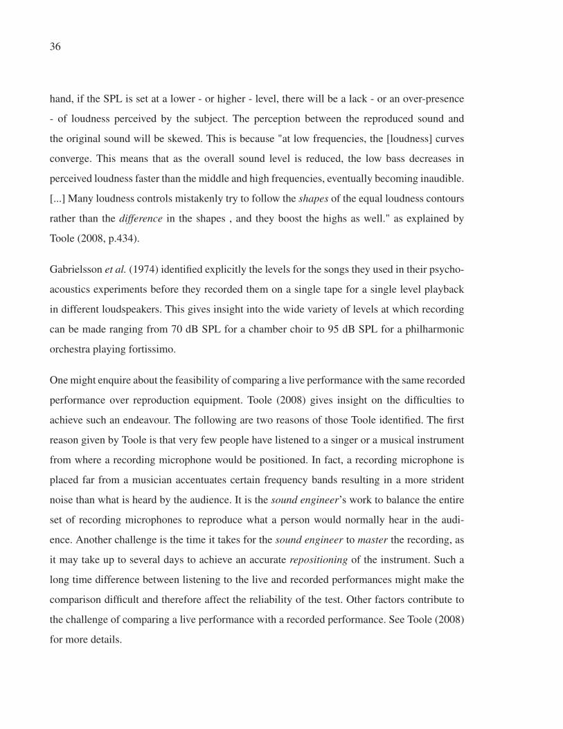
36
hand, if the SPL is set at a lower - or higher - level, there will be a lack - or an over-presence
- of loudness perceived by the subject. The perception between the reproduced sound and
the original sound will be skewed. This is because "at low frequencies, the [loudness] curves
converge. This means that as the overall sound level is reduced, the low bass decreases in
perceived loudness faster than the middle and high frequencies, eventually becoming inaudible.
[...] Many loudness controls mistakenly try to follow the shapes of the equal loudness contours
rather than the difference in the shapes , and they boost the highs as well." as explained by
Toole (2008, p.434).
Gabrielsson et al. (1974) identified explicitly the levels for the songs they used in their psycho-
acoustics experiments before they recorded them on a single tape for a single level playback
in different loudspeakers. This gives insight into the wide variety of levels at which recording
can be made ranging from 70 dB SPL for a chamber choir to 95 dB SPL for a philharmonic
orchestra playing fortissimo.
One might enquire about the feasibility of comparing a live performance with the same recorded
performance over reproduction equipment. Toole (2008) gives insight on the difficulties to
achieve such an endeavour. The following are two reasons of those Toole identified. The first
reason given by Toole is that very few people have listened to a singer or a musical instrument
from where a recording microphone would be positioned. In fact, a recording microphone is
placed far from a musician accentuates certain frequency bands resulting in a more strident
noise than what is heard by the audience. It is the sound engineer’s work to balance the entire
set of recording microphones to reproduce what a person would normally hear in the audi-
ence. Another challenge is the time it takes for the sound engineer to master the recording, as
it may take up to several days to achieve an accurate repositioning of the instrument. Such a
long time difference between listening to the live and recorded performances might make the
comparison difficult and therefore affect the reliability of the test. Other factors contribute to
the challenge of comparing a live performance with a recorded performance. See Toole (2008)
for more details.

37
Figure 1.12 Circle of confusion describing the conundrum of sound reproduction.
[Adapted with permission from Toole (2008)]
1.2.4 Ear canal sealed by the earphone
Sealing the ear canal with an earphone produces two impacts on the performance of earphones
and is to be taken into account. The first is the attenuation of outside noises. The second is the
residual sealed ear canal volume which changes the impedance of the ear canal, as presented in
section 1.1.4, and has a resulting effect on the earphone’s frequency response. The attenuation
is tested by different methods: Real Ear Attenuation at Threshold (REAT), Microphone In
Real Ear (MIRE), Field-Microphone In Real Ear (F-MIRE), etc. However, the REAT is still
considered the "gold standard" of attenuation measurement, as presented by Berger (2005).
Figure 1.13 presents the attenuation of EERS, a custom fit earphone, by Sonomax® (Mon-
tréal, Canada). The earphone was tested on 20 subjects, 2 times (N=40) for 7 frequencies. The
straight line is the normal distribution expected from the sampling while the individual sub-
jects’ data is represented by markers. It can be seen that some subjects get amplification for

38
the 125 Hz, 250 Hz and 500 Hz octave-bands corresponding to a negative attenuation. This is
likely due to resonance of the coupling of the earplug with the subjects’ ear canals.
−5 0 5 10 15 20 25 30 35 40 450.010.020.050.10
0.25
0.50
0.75
0.900.950.980.99
Attenuation (REAT) [dB]
Prob
abili
ty
125 [Hz]250 [Hz]500 [Hz]1 [kHz]2 [kHz]4 [kHz]8 [kHz]
Figure 1.13 Normal probability plot for 7 octave band frequencies of the attenuation in
dB of custom fit earphones tested according to ANSI S12.6.
1.2.4.1 Increase of the Signal-to-Noise Ratio
A Signal-to-Noise Ratio (SNR) is a measure of the square of the amplitude of a signal over
the square of the amplitude of the background noise. The attenuation offered by earphones
modifies the listening behaviour of the wearer in a positive way. It allows a safer listening
level and, as a result, helps preserve one’s hearing, as reported by Voix et al. (2008). They
concluded that "the preferred listening level (PLL) is, for a given individual, essentially driven
by the background noise level." The first impact of the attenuation of sound by the earphone is
the increase of the SNR between the sound played back by the earphones (inside the ear canal)
and the ambient noise (outside the earphone). Voix et al. (2008) concluded that: "Using a
simple statistical analysis on existing published data, the percentage of wearers using a regular
non-isolating earphone exposed to a potentially dangerous noise dose has been established
to 45.1%. The use of the proposed custom isolating earphone would lead theoretically to a
substantial decrease (down to 3.1%) of the percentage of users putting their hearing at risk."

39
The attenuation of an earphone is measured using the same standard as a hearing protector and
the International Electrotechnical Commission (2010a) refers to ISO 4869-1 for the attenuation
testing.
As a complement to the observations of Voix et al. (2008), Shimokura and Soeta (2012) "ex-
amine the listening level of music through earphones in the noisy environment of a train car".
They took the stringent hearing protection recommendations of the WHO, recommending a
limit of 75 dB(A) for a 8-h period and 70 dB(A) for a 24-h period and compared the impact on
the noise level generated by the train car to the level generated by the intra-concha earphone,
as set by the subject and measured by a IEC 711 coupler (see section 2.2). They concluded that
the optimum level of music volume heard through a headphone increased as the train car noise
level becomes higher. These results correlate with Voix et al. (2008). Furthermore, a study by
Keith et al. (2011) in a quieter environment found the same trend, that is, playback levels are
driven by background noise.
Relating to previous studies establishing the relation between the listening levels and the signal-
to-noise ratio, it seems that people do not necessarily listen to music at higher levels with ear-
phones than on loudspeakers. The main indicator is the difference between the outside noise
and the inside noise, so an attenuation of 20 dB or more provides sufficient SNR for the back-
ground noise not to have an influence on the preferred listening level. This will greatly help
reduce the potential hearing loss of individuals who use earphones.
1.2.4.2 Effect of sealing the ear canal on the low frequencies reproduction
As presented in Borwick et al. (2001, p.596) and explored again by Poldy (2006), creating
a seal between the earphone and the ear canal has a direct impact on the reliability of the
frequency response for low frequencies reproduction.
p = ξωρc (1.1)
In equation 1.1, the proportionality of the increase of the displacement (ξ) to match the decrease
in frequency (ω) is explicit in order to keep the same pressure (p). So, for a same excursion of
40
the diaphragm, a cut-off frequency will appear if there is a leak. This phenomenon is a likely
reason why people often comment about the lack of bass in the earphone sound reproduction.
102 103 10430
35
40
45
50
55
60
65
70
75
80
Frequency (Hz)
Am
plitu
de (d
B S
PL)
Sealed earphone, properly insertedNon−sealed earphone, properly insertedNon−sealed earphone, wrongly inserted
Figure 1.14 The effect on the frequency response function of a leak in the earpiece.
Figure 1.14 presents the frequency response function of three typical cases for an earphone
designed to seal the ear canal: a properly sealed earphone, a properly inserted earphone with
a small leak and a wrongly inserted, not sealed earphone. Thus, by sealing the ear canal, the
diaphragm displacement acts like the displacement of a piston in a closed volume (Vx). The
displacement reduces, or increase, the volume of a known quantity, increasing the pressure (Px)
regardless of the frequency. In a first approximation, the increase in pressure, proportionally to
a reference pressure of 20 μPa, defines the sound pressure level experienced by a subject.
P1Vγ1 = P2V
γ2 (1.2)

41
This approximation does not take into account the displacement of the ear canal from sound
pressure and other artifacts linked to the masking of sound by human body noise, accentuated
by sealing the ear with an earphone.
1.3 On the definition of an earphone target frequency response
Many attempts to define a target frequency response have been made by studying the real ear
transfer function in different fields. The resulting frequency responses have been evaluated for
sound quality with psycho-acoustic tests. This method seems to be the preferred way to achieve
accurate sound reproduction with earphones, essentially because the most important aspects are
the signal at the eardrum and how it is perceived.
1.3.1 Issues related to earphone sound reproduction
Before establishing what is the preferred frequency response for an earphone, it is of interest
to know the main issues raised about the sound reproduction with earphones. Sakamoto et al.
(1976) listed two of the main issues pertaining to earphone sound reproduction:
• The sound image remains "within" the area of the head;
• there is a lack of richness in the quality of reproduced sound.
The richness of the quality of reproduced sound greatly improved since the publication of their
article, but the challenge of the "out-of-the-head" music listening is still very present, even in
today’s publications. Sakamoto et al. (1976) listed possible reasons contributing to the aspect
of in-head listening (IHL):
• Lack of effect of head movement relative to the sound;
• the absence of bone conduction, [a phenomenon by which sound travels to the auditory
system by a solid path and not only by the aerial path] ;
• distortion in the [sound reproduction chain, including headphones];
• incorrect transfer function from the earphones to the [eardrum].

42
The lack of effects related to head movement, as covered in section 1.1.2.2 is inherent to ear-
phone use. Compensation for this can be achieved through a complex convolution of sound and
head tracker sensors, not covered here because this thesis analyzes time invariant frequency re-
sponses of earphone. Bone conduction impact as an indicator of sound quality seems of minor
importance compared to the aerial path for most of the listening experience. The distortion
levels are one or two orders of magnitude less important, as presented in section 2.2. The in-
correct transfer function from the earphone to the ear is deemed to have the most impact on
sound quality, as explored in section 1.3.2. The approach of Sakamoto et al. (1976) to compen-
sate for the in-head sound location consists in superimposing a delayed signal to the original
signal, to match the delay present in a room with loudspeakers playing and achieve the acoustic
ratio (AR) defined as:
AR =ER
ED
(1.3)
Where ER is the acoustic energy density of reflected sound and ED, the acoustic energy density
of direct sound. This approach is a basic lead, lag method as presented in section 1.1.2.2.
A research conducted by Toole (1984), who undertook a very comprehensive work to define
what is implied in the acoustics and psycho-acoustics of headphones, states that:
This very specific kind of performance is not likely to happen by accident. [...]
Mainly the evidence suggested that in-head localization occurred when the acous-
tical signals at the ears did not fit a familiar pattern. [...] This is simply loudspeaker
stereo with the loudspeakers whispering in the ears. Sound images (as opposed to
vague spatial impressions) located between the ears will occur only for highly-
correlated sounds arriving at the ears within about 0.7 ms of each other. [...] How-
ever, at the present time serious listeners are likely to find the use of headphones
an unnatural if not an unpleasant experience."
He then concludes: "it is not only that the products fail to meet the proper objectives; the proper
objective has not been defined."
43
1.3.2 Comparison of studied frequency response
Many studies were performed to find the frequency response that would elicit a virtual repro-
duction from a stereo signal. These studies will be presented in a chronological order to ease the
relation and concerns of latter studies in relation to former ones. Also, this section discusses the
earphone and headphone frequency response function. Since most of the measurements were
performed in the vicinity of the eardrum or at the entrance of the ear canal, it is assumed that it
is applicable for circumaural as well as insert earphones.
In their study, Gabrielsson et al. (1990) shaped the frequency response using signal processing
to evaluate the impact of a band-limited gain on the preference of subjects in music reproduc-
tion. Their results are summarized in Table 1.6, presenting many perceptual descriptors as well
as their impact on sound quality. It is a vivid representation of the complexity of audio quality
assessment illustrating that it is more complex than identifying a generic frequency response.
This study looked at jazz music, pink noise and the female voice and finds different results for
each type of stimulus. Other type of music might yield different conclusions on the preferred
frequency response of earphones. Thus, it would be of interest to adjust the target frequency
response presented in this section if the earphone is to be dedicated to a specific music type.
One of the first studies about earphones that used a probe microphone and a coupler to relate
a real ear acoustical load to a frequency response came from Villchur (1969), who published a
study on how to calibrate a headphone in free-field. He readily noted the effect of the cushion-
fit variations and the acoustic gain of the earphone. His study was performed for circumaural
type earphones. In the same line of thought, Toole (1984) demonstrated what a good and a
poor earphone frequency response would be, reaching conclusions similar to Villchur (1969)
in many aspects. He also noted the possibility of using the diffuse-field approach for com-
pensation. Theile (1986) concludes that "a flat diffuse-field response, measured with a probe
microphone in the auditory canal of real ears, defines the optimum correct performance".
In a complementary approach, Møller et al. (1992) measured the HRTF of 24 subjects where
they found very large variations in amplitude for frequencies as low as 2.5 kHz. Then, Møller

44
et al. (1995a) established the design criteria for headphones by measuring the diffuse-field and
free-field transfer function. They observed that "above 8 kHz quite large variations are seen -
5-10 dB for the diffuse-field and slightly higher for the free-field calibration. The peaks and
dips of this variation can be seen in the work of Hammershøi and Møller (1996) in which they
measured at different sound transmission positions to and within the ear canal. The variability
in the multiple options leaves place for an educated decision on what is a good frequency re-
sponse for an earphone or a bad one. As stated by Borwick et al. (2001, p.653), "a palate of
different frequency responses is available to cater for individual preferences, and each manu-
facturer has its own headphone philosophy with frequency responses ranging from flat to free
field and beyond." However, that variability is not very high below 8 kHz, giving leave for
"the assumption in [Lorho (2009)]that an optimal perceived quality exists for a specific com-
bination of parameters values." Lorho (2009) studied the effect of the 3 kHz and 11 kHz peak
amplitude by asking 80 subjects to assess what they preferred. His experiment opened a new
chapter in earphones target frequency response by concluding that a 3 dB amplitude at 3.1 kHz
is optimal. An exploration of other options by Fleischmann et al. (2012) proposed that Lorho’s
target amplitude is not optimal. The former showed by their results from different groups that
no specific frequency response would yield unequivocal results.
This observation can be also found in Olive and Welti (2012a); Olive et al. (2013). They
have shown by their results that other options (like the diffuse-field approach by Møller et al.
(1995a)) cannot be discarded altogether since their mean preference, even if lower, are still
rated to a level leaving room for discussion. Olive and Welti (2012a); Olive et al. (2013) con-
cluded that listeners prefer a non-coloured frequency response with a good spectral balance.
They defined a frequency response based on the measurement explained in section 1.1.2.2 and
concluded that the frequency response they identified offers the best performance. Essentially,
their frequency response curve is similar to the frequency response presented in Figure 1.5 with
a 3 kHz amplitude of 10 dB.
This conclusion is based on several factors. One of these is the sequential contraction bias: "the
preceding stimuli will have an influence on the assessment of the succeeding stimuli. So the
45
general rule for context effects is that humans adapt to the environment that they are presently
in. This means that evaluations of impressions will not - as a general rule - be absolute, but
will always be a function of the surroundings – that is the context." as stated by Bech and
Zacharov (2006, p.87). This problem has been greatly dampened by Olive’s randomization of
stimulus and double-blind testing. Although, no study is free of the bias effect: "A bias effect
that is independent of context would be the general conservative nature of subjects to save
parts (upper and lower) of the rating range to be assigned to the yet unknown stimuli." Again,
Olive and Welti (2012b) used trained listeners for their experiment, meaning that these subjects
have a sense of magnitude on sound quality. They have a knowledge of the vocabulary and are
familiar with what stimulus variations to assess, so it can be assumed that they use the full range
of the scale. Using a trained panel of listeners creates other biases, like the transfer bias, where
they refer extensively to their background instead of focusing on the samples in the study.
Unfortunately, the most important factor is that a large number of subjects are needed, typically
in the range of hundreds, to obtain statistically valid results. The reason is that subjects differ
in hearing abilities, interests, ability to work as test subjects, and so on, as noted by Bech
and Zacharov (2006, p.121). This is a very important limitation of most of the studies on
earphone sound signature: they rely on several subjects and several variations of variables. It
limits the relevance of most studies on audio quality assessment. Experiments by Olive and
Lorho had more subjects on their panel, and their conclusions are also the most challenged by
other authors.
1.4 Conclusions on the psycho-acoustics of earphone
In this chapter, the fundamentals of psycho-acoustics related to earphones are presented. The
large variability of the coupling between the earphone and the ear is identified. This includes
several effects, such as the impact of occluding the ear on the bass reproduction, that contribute
to the perceived quality of earphones. The words used to describe this impact, for example thin,
boomy, and full is listed for each of the attributes of sound perception.

46
This chapter also highlights the differences between listening to a distant source and listening
with earphones. The impact of the HRTF approximation on the perceived quality of earphones
is considered very important since it is a natural effect people are naturally accustomed to. This
is why many studies try to recreate a frequency response based on this concept. However, at the
time of the writing, no frequency response function could be said to constitute the definitive
target response. The author concludes that this is most likely because of the inter/intra sub-
ject variability, something less prevalent for loudspeakers. Another factor contributing to this
variability is the coupling between the ear and the earphone, something not experienced with
loudspeakers. The only agreement of all the studies presented in this chapter is the need for a
3 kHz amplitude boost in order to recreate the resonance of the open ear canal.

47
Tab
le1.6
Aggre
gat
ion
of
the
work
pre
sente
din
Gab
riel
sson
etal
.(1990):
The
impac
tof
loudnes
sle
vel
(70
and
80
dB
(A))
com
bin
edw
ith
oth
erper
ceiv
eddim
ensi
ons
from
0(m
inim
um
)to
10
(max
imum
)on
earp
hone
per
ceiv
edqual
ity
for
jazz
musi
c
[Ret
riev
edfr
om
figure
s]
Impa
ctof
fact
ors
Dim
ensi
onD
escr
iptio
nL
evel
Flat
Low
filte
rM
idhi
ghfil
ter
Hig
hfil
ter
Bri
ghtn
ess†
Bri
ght
[10]
toD
ull
,D
ark
[0]
Hig
h5.9
3.9
6.3
6.5
Low
5.5
4.5
5.2
6.9
Cla
rity
Cle
ar,D
isti
nct
,P
ure
[10]
toC
lose
,sh
ut
up
[0]
Hig
h6.9
6.5
7.2
‡7.2
Low
5.6
55.9
‡6.5
Fid
elit
y†
Sim
ilar
toori
gin
alP
erfe
ct[1
0]
toN
ot
atal
l[0
]H
igh
6.5
5.3
5.4
5.5
Low
5.2
4.9
5.2
‡5.3
‡F
ull
nes
sM
axim
um
full
nes
s[1
0]
tover
yth
in[0
]H
igh
6.3
7.2
6‡
5.2
‡L
ow
55.8
5‡
4.8
Loudnes
sV
ery
loud
[10]
tover
yso
ft[0
]H
igh
66.5
7.5
7.2
Low
44.8
4.5
4.8
Nea
rnes
sV
ery
Nea
r[1
0]
toV
ery
Dis
tant
[0]
Hig
h6.2
6.8
76.9
Low
44.5
4.8
4.8
Soft
nes
sV
ery
soft
[10]
toV
ery
Shar
p[0
]H
igh
5.5
5.9‡
3.5
3
Low
66.5
6‡
5.3
Spac
iousn
ess
Ver
yopen
[10]
toV
ery
close
[0]
Hig
h7
66.4
7
Low
4.6
4.6‡
5‡
5.6
‡
Note
:F
requen
cyra
nge:
[20
Hz
toan
anti
-ali
asin
glo
w-p
ass
filt
erse
tat
6.7
kH
z.A
mpli
fica
tion
filt
er]
Des
crip
tion
of
filt
ers:
Low
pas
s
filt
er[+
9dB
bel
ow
200
Hz,
+3
dB
at700
Hz]
,m
idhig
hban
dpas
sfi
lter
[+9
dB
around
1kH
z(+
3dB
at420
Hz
and
2kH
z)],
hig
h
ban
dpas
sfi
lter
[+9
dB
around
4kH
z,+
3dB
at2.2
kH
zan
d5.8
kH
z].†I
ndic
ates
anon-s
ignifi
cant
dif
fere
nce
bet
wee
nle
vel
sfo
rth
e
sam
efi
lter
,as
com
pute
dby
the
auth
ors
.‡i
ndic
ates
anon-s
ignifi
cant
var
iati
on
com
par
edto
the
flat
resp
onse
,
asco
mpute
dby
the
auth
ors
.

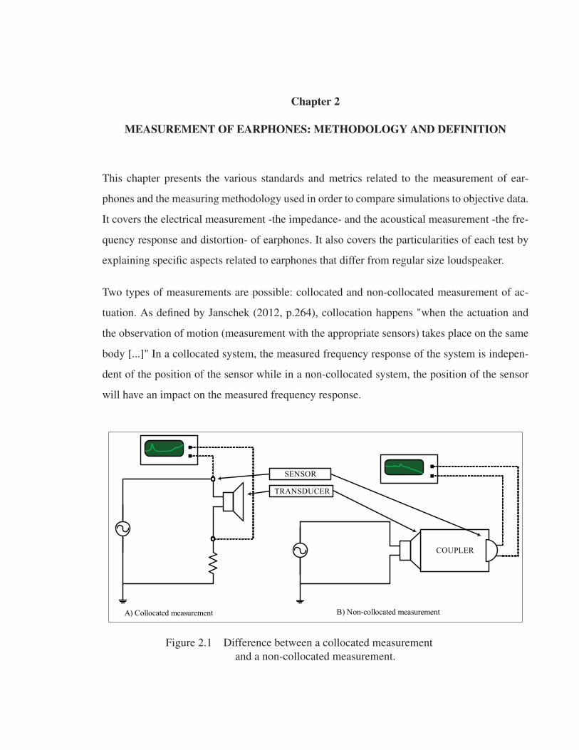
Chapter 2
MEASUREMENT OF EARPHONES: METHODOLOGY AND DEFINITION
This chapter presents the various standards and metrics related to the measurement of ear-
phones and the measuring methodology used in order to compare simulations to objective data.
It covers the electrical measurement -the impedance- and the acoustical measurement -the fre-
quency response and distortion- of earphones. It also covers the particularities of each test by
explaining specific aspects related to earphones that differ from regular size loudspeaker.
Two types of measurements are possible: collocated and non-collocated measurement of ac-
tuation. As defined by Janschek (2012, p.264), collocation happens "when the actuation and
the observation of motion (measurement with the appropriate sensors) takes place on the same
body [...]" In a collocated system, the measured frequency response of the system is indepen-
dent of the position of the sensor while in a non-collocated system, the position of the sensor
will have an impact on the measured frequency response.
COUPLER
B) Non-collocated measurement
TRANSDUCER
SENSOR
A) Collocated measurement
Figure 2.1 Difference between a collocated measurement
and a non-collocated measurement.

50
2.1 Collocated measurement of earphones
The main collocation measurement of an earphone is the impedance/frequency characteristics.
The International Electrotechnical Commission (2010a) requires a complete measurement of
the impedance for a frequency range of 20 Hz to 20 kHz (the hearing spectrum). The input
signal shall be a variable sinusoidal voltage or current at an amplitude allowing for linear
operation of the transducer. This requirement might be more difficult to achieve for balanced-
armature transducers because their building architecture is based on the cantilever principle,
as extensively explained by Jensen (2009); Jensen et al. (2011). The impedance measurement,
by its collocation nature, can also be used as a basis to determine the modelling parameters of
a transducer. The most renowned modelling method based on the impedance measurement is
the small-signal analysis of a loudspeaker. The small signal analysis is the process by which
nonlinear systems are approximated by a linear equivalent for an input signal amplitude where
the nonlinear and the linear system approximation yield similar responses. For the equations
of the small signal parameters from the impedance measurement, refer to Appendix I.
102 103 10431.5
32
32.5
33
33.5
34
34.5
35
Frequency [Hz]
Impd
eanc
e [O
hm]
Figure 2.2 Modulus of the impedance curve of a micro-loudspeaker measured with
the method presented in D’Appolito (1998).

51
2.1.1 Application to moving-coil micro-loudspeaker
As stated previously, the small-signal is widely used and extensively explained in the literature
e.g. : Struck (1987), D’Appolito (1998). One could comprehend a small signal as a signal that
yields a linear (k) incremental pressure output (Pout) for the studied frequency band in relation
to the electrical input (Vin).
k ∝ Pout
Vin
(2.1)
An important difference exists when a moving-coil micro-loudspeaker is measured, compared
to a larger size driver, a generic name for electro-mechanical machines also used for loud-
speakers, for the equivalent compliance volume parameter(VAS
[Nm
]). The equivalent volume
parameter is an equivalent volume of air acting upon a piston of surface area (SD [m2]) that
represents the same compliance as the compliance - reciprocal of stiffness - of the driver’s sus-
pension. One of the most renown method to measure the VAS is by the close-volume method.
1000 2000 3000 4000 5000 6000 8000 1000032.5
33
33.5
34
34.5
35
Frequency [Hz]
Impe
danc
e [O
hms]
Free Air2cc Closed Volume Load
Figure 2.3 Impedance curve of a moving-coil micro-loudspeaker measured in free
air and with a 2cc closed volume air load.
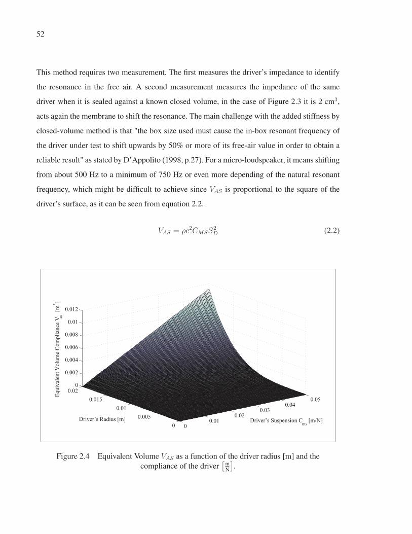
52
This method requires two measurement. The first measures the driver’s impedance to identify
the resonance in the free air. A second measurement measures the impedance of the same
driver when it is sealed against a known closed volume, in the case of Figure 2.3 it is 2 cm3,
acts again the membrane to shift the resonance. The main challenge with the added stiffness by
closed-volume method is that "the box size used must cause the in-box resonant frequency of
the driver under test to shift upwards by 50% or more of its free-air value in order to obtain a
reliable result" as stated by D’Appolito (1998, p.27). For a micro-loudspeaker, it means shifting
from about 500 Hz to a minimum of 750 Hz or even more depending of the natural resonant
frequency, which might be difficult to achieve since VAS is proportional to the square of the
driver’s surface, as it can be seen from equation 2.2.
VAS = ρc2CMSS2D (2.2)
00.01
0.020.03
0.040.05
00.005
0.010.015
0.020
0.002
0.004
0.006
0.008
0.01
0.012
Driver’s Suspension Cms
[m/N]Driver’s Radius [m]
Equi
vale
nt V
olum
e C
ompl
ianc
e V as
[m
3 ]
Figure 2.4 Equivalent Volume VAS as a function of the driver radius [m] and the
compliance of the driver[
mN
].
53
Given the small diameters and the difficulty to properly adjust the air volume in front of the
driver, the 50% criteria might be difficult to achieve and not repeatable. As presented in Figure
2.4, the driver radius has more impact on the selection of the air volume than the compliance
of the membrane. So, for a low compliance, small radius driver, the VAS necessary to achieve
adequate results is very small. For example, the micro-loudspeaker used in the article presented
in section 3.3, is of an equivalent radius of .006 m and the driver’s suspension compliance is
13.41× 10⁻³ mN
, so a volume of the order of magnitude of 10−6 m3 is necessary. In this case, an
alternative is to limit the resistance from air to ease the displacement of the diaphragm and shift
the peak to a lower frequency to achieve the 50% difference between peaks. This means that
for the same driver, a 500 Hz peak has to be shifted down to approximately 333 Hz to reach
the same accuracy. This peak shift is possible by placing the driver into a sealed enclosure
and lowering the pressure in order to achieve the 50% mark. VAS is an equivalent parameter
characterizing how a loudspeaker behaves and is also used to change the load, and the resulting
impedance. RE , the voice-coil resistance, and LE , the voice-coil inductance, are more com-
plex to measure since they are frequency dependent. D’Appolito (1998, p.32) explains how to
compute them from the impedance measurements. It requires access to the impedance curve
measurement in Figure 2.2. RE is the real part of the impedance curve and is equivalent to RDC
until the heat loss becomes significant, then RE increases and becomes frequency dependent.
The voice-coil inductance, LE , can be computed using equation 2.3.
LE =1
4π2f 20CES
=0.0253
f 20CES
(2.3)
Equation 2.3 is valid at the second zero phase, which can be seen in Figure 2.5, and is where the
voice-coil resistance and inductance creates an impedance rise. In order to determine voice-coil
inductance with reasonable accuracy at frequencies above the second zero phase point, both
the magnitude and phase of the driver impedance are required. It can be computed using the
following steps:

54
102 103 104
40
60
80
100
120
Am
plitu
de [d
B S
PL]
102 103 104
−100
0
100
Frequency [Hz]
Phas
e an
gle
[Deg
ree]
2nd ZeroPhase
Figure 2.5 Frequency response function of an earphone (top) and the phase (bottom)
with the second zero phase identified.
a. At each frequency of interest, compute the reactive component of driver impedance
where |Z| is the impedance magnitude and θ is the impedance phase angle;
X = |Z|sinθ (2.4)
b. At each frequency f, for which LE is desired, correct the reactance determined in step a.
for the effect of CES using:
XL = X +1
2πfCES
= X +0.1592
fCES
(2.5)
c. Compute LE using:
LE =0.1592XL
f(2.6)
Other methods using curve match - or an empirical transfer function - can also be used depend-
ing on processing power available.
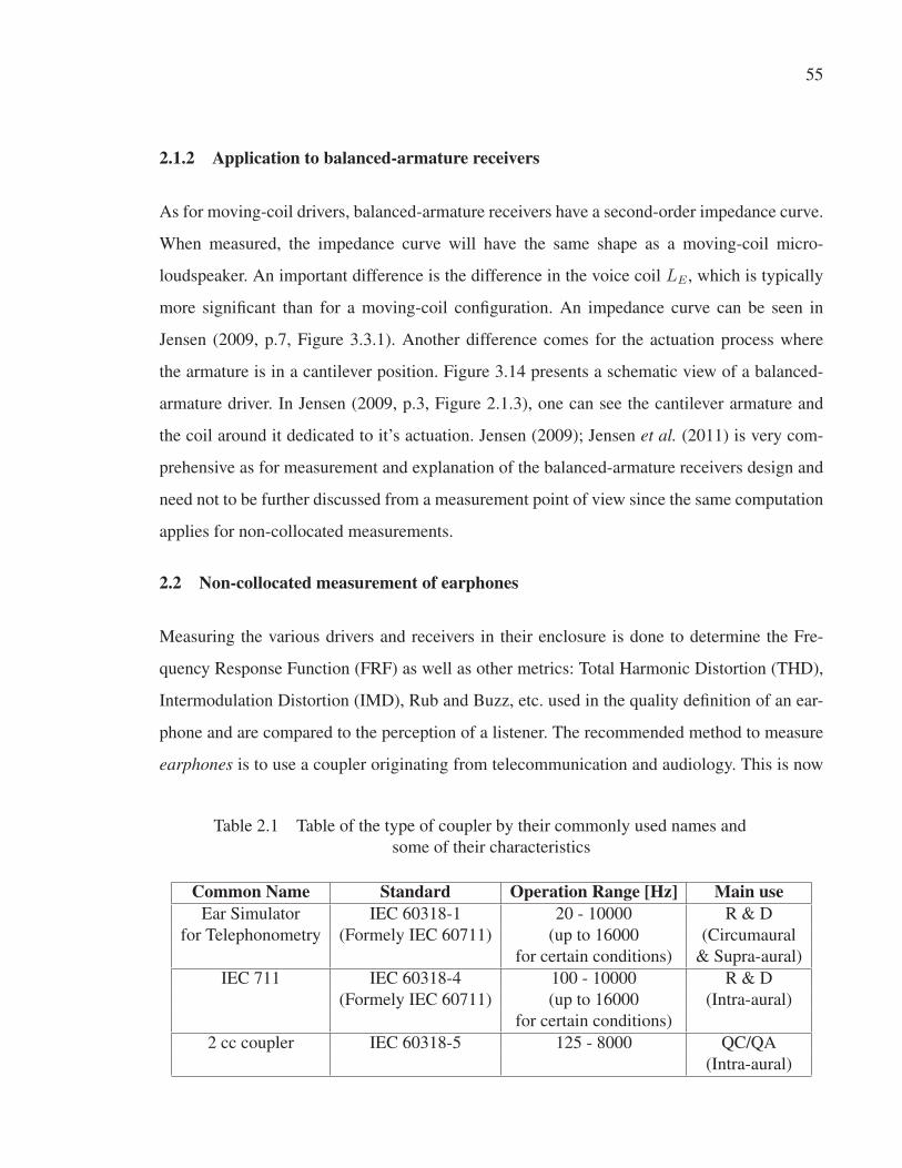
55
2.1.2 Application to balanced-armature receivers
As for moving-coil drivers, balanced-armature receivers have a second-order impedance curve.
When measured, the impedance curve will have the same shape as a moving-coil micro-
loudspeaker. An important difference is the difference in the voice coil LE , which is typically
more significant than for a moving-coil configuration. An impedance curve can be seen in
Jensen (2009, p.7, Figure 3.3.1). Another difference comes for the actuation process where
the armature is in a cantilever position. Figure 3.14 presents a schematic view of a balanced-
armature driver. In Jensen (2009, p.3, Figure 2.1.3), one can see the cantilever armature and
the coil around it dedicated to it’s actuation. Jensen (2009); Jensen et al. (2011) is very com-
prehensive as for measurement and explanation of the balanced-armature receivers design and
need not to be further discussed from a measurement point of view since the same computation
applies for non-collocated measurements.
2.2 Non-collocated measurement of earphones
Measuring the various drivers and receivers in their enclosure is done to determine the Fre-
quency Response Function (FRF) as well as other metrics: Total Harmonic Distortion (THD),
Intermodulation Distortion (IMD), Rub and Buzz, etc. used in the quality definition of an ear-
phone and are compared to the perception of a listener. The recommended method to measure
earphones is to use a coupler originating from telecommunication and audiology. This is now
Table 2.1 Table of the type of coupler by their commonly used names and
some of their characteristics
Common Name Standard Operation Range [Hz] Main useEar Simulator IEC 60318-1 20 - 10000 R & D
for Telephonometry (Formely IEC 60711) (up to 16000 (Circumaural
for certain conditions) & Supra-aural)
IEC 711 IEC 60318-4 100 - 10000 R & D
(Formely IEC 60711) (up to 16000 (Intra-aural)
for certain conditions)
2 cc coupler IEC 60318-5 125 - 8000 QC/QA
(Intra-aural)

56
standardized by several IEC standards which defines the measurement tools as well as the mea-
surement methods. Three of the couplers that are standardized as earphone measurement tools
are presented in table 2.1. Figure 2.6 presents, as an example, the fine band transfer function re-
sponse between the original signal (white noise) and the coupler (IEC 60318-4) signal recorded
by a data acquisition system and processed with MATLAB.
102 103 104
−60
−40
−20
0
Am
plitu
de [d
B]
102 103 1040
0.2
0.4
0.6
0.8
1
Coh
eren
ce fa
ctor
Frequency [Hz]
Figure 2.6 Exemple of a transfer function between the electrical input and the measured
SPL (top) and coherence (bottom) of an earphone measured on an IEC 60318-4 coupler.
The coherence between the input signal and the recorded signal by the coupler is not unity
below 100 Hz, as expected from the standard. Toole (1984) noted that "in general it seemed
reasonable to rely on replica-ear measurements at frequencies above 300-500 Hz". While the
improvement of measurement tools is noticeable, reliable coherence of measurements under
100 Hz is still very difficult to achieve. This is principally because of noise pollution which
is very difficult to eliminate from the surroundings. The use of a room especially designed to
eliminate outside noise pollution, such as an anechoic chamber, greatly improve the coherence.
When such an environment is available, it is necessary to confirm if coherence can be achieve
under 100 Hz on a case-by-case basis. The IEC 60318-1 coupler is efficient down to 20 Hz
57
because it is entirely made of steel which is less affected by the outside noise pollution than
when coupled with a rubber ear replica.
For non-collocated measurement of earphones, the following testing conditions should be cal-
ibrated to ensure the validity of the measurement:
• A standardized coupler is used as a measurement tool. The selection of the coupler is
based on the type of earphones to be measured, see Table 2.1;
• the coupler and the related equipment are calibrated with a sinusoidal source of a known
frequency to 94 dB (1 Pa when referenced to 20 μPa). The International Electrotechnical
Commission (2010a) requires 500 Hz as a reference signal. However, most commercial
calibrators are set to produce a 1 kHz reference sinusoidal wave since it is defined as
the preferred reference frequency by the International Organization for Standardization
(1997);
• the earphone is inserted - or pressed against the head - with a known application force,
ideally representative of the average force subjects would use to insert the earpiece.
As for any other type of measurement, the main purpose of the control of these variables is to
ensure a reproducibility of the tests, when a variable is changed, or for an independent tester to
be able to replicate the measurements.
2.2.1 Frequency Response Function
A frequency response function is a dependent magnitude plot of a certain physical quantity as
a function of the frequency of a known, and generally fixed, stimulus. For more details about
the nature of the frequency response functions, see section 3.1.1. Frequency response function
are typically used in earphone measurement to:
• Assess, through correlation, the electro-acoustical output to the audio quality of the sys-
tem;
• determine the natural frequency and harmonics of a system;
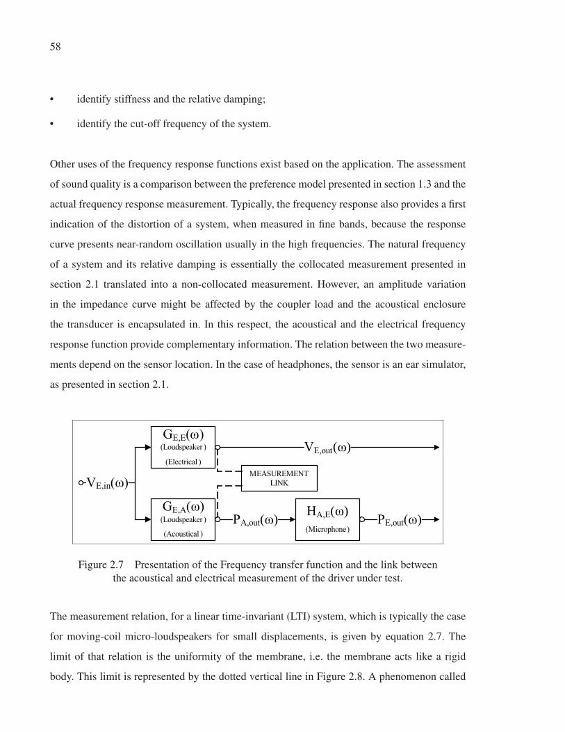
58
• identify stiffness and the relative damping;
• identify the cut-off frequency of the system.
Other uses of the frequency response functions exist based on the application. The assessment
of sound quality is a comparison between the preference model presented in section 1.3 and the
actual frequency response measurement. Typically, the frequency response also provides a first
indication of the distortion of a system, when measured in fine bands, because the response
curve presents near-random oscillation usually in the high frequencies. The natural frequency
of a system and its relative damping is essentially the collocated measurement presented in
section 2.1 translated into a non-collocated measurement. However, an amplitude variation
in the impedance curve might be affected by the coupler load and the acoustical enclosure
the transducer is encapsulated in. In this respect, the acoustical and the electrical frequency
response function provide complementary information. The relation between the two measure-
ments depend on the sensor location. In the case of headphones, the sensor is an ear simulator,
as presented in section 2.1.
GE,A(ω)(Loudspeaker )
(Acoustical )PA,out(ω)
GE,E(ω)(Loudspeaker )
(Electrical )VE,out(ω)
VE,in(ω)
HA,E(ω)(Microphone)
PE,out(ω)
MEASUREMENT LINK
Figure 2.7 Presentation of the Frequency transfer function and the link between
the acoustical and electrical measurement of the driver under test.
The measurement relation, for a linear time-invariant (LTI) system, which is typically the case
for moving-coil micro-loudspeakers for small displacements, is given by equation 2.7. The
limit of that relation is the uniformity of the membrane, i.e. the membrane acts like a rigid
body. This limit is represented by the dotted vertical line in Figure 2.8. A phenomenon called

59
the cone breakup may occur, this means that not only does the membrane have axial modes
when actuated, but the actuation force and the membrane movement become out of phase with
radial modes. A demonstration of the measurements that characterizing a cone breakup has
been made by Klippel and Schlechter (2006).
GE,E(ω) =VE,out(ω)
VE,in(ω)⇔ GE,A(ω) =
PE,out(ω) · VE,in(ω)
HA,E(ω)(2.7)
Where VE,in(ω) is the voltage used to stimulate the DUT. VE,out(ω) is the voltage across the
driver. PA,out(ω) is the acoustical pressure generated by the loudspeaker and measured by the
microphone. PE,out(ω) is the voltage generated by the microphone when stimulated by the pres-
sure PA,out(ω). The transfer function G and H are those of the loudspeaker and microphone,
respectively. Two dotted boxes in in Figure 2.8 identifies artefacts in the frequency response
that could be related by the relation presented in equation 2.7.
102 103 104859095
100105110
Am
plitu
de [d
B S
PL]
102 103 10428.22930313233
Impe
danc
e [O
hms]
102 103 104−180−90
090
180
Phas
e A
ngle
[Deg
ree]
Frequency [Hz]
Frequency ResponseImpedance
Figure 2.8 Presentation of the frequency response of a micro-loudspeaker measured in a
IEC 60318-4 coupler and the impedance measurement of the same micro-loudspeaker
with the IEC 60318-4 coupler as air load.
The International Electrotechnical Commission (2010a) allows for a field comparison of the
frequency response measured by test subjects using the loudness matching method. This fre-

60
quency response would be a loudness response of the earphone, not an SPL frequency response.
It is of interest, but also introduces more variability with problems such as the "missing 6 dB"
and the inter/intra subject variability, as explained in section 1.2.2. As recommended by the
International Electrotechnical Commission (2010a), the frequency response function of the
pressure output is measured using a low to high swept-frequency for the frequencies between
20 Hz and 20 kHz. The result is then plotted on a scale in which a 50 dB amplitude is of the
same size as a decade on the frequency axis. In other terms, to cover two decades (20 Hz to
20 kHz), the amplitude of the plot will be of 100 dB.
2.2.2 Harmonic Distortion
For an earphone, the International Electrotechnical Commission (2010a) establishes the spec-
ification of the harmonic distortion measurement and requests two measurements: harmonic
distortion by order (HD) and Total Harmonic Distortion (THD). Temme et al. (2012) explain
that "in an electromagnetic driver, the force factor of the motor, the electrical inductance of the
voice coil and the stiffness of the cone suspension are nonlinear functions of the cone excursion.
A strong 2nd harmonic will indicate an asymmetry of these characteristics along the excursion
range and/or poor centering of the voice coil in the magnetic gap. A strong 3rd harmonic will
reveal a symmetrical alteration at both ends of the excursion range." Further details can be
found in the work of Cunningham (1949). The equations to calculate the harmonic distortion
are:
• harmonic distortion of the nth order (n = 2 or 3), which is the ratio of the output sound
pressure Pf at n times the input frequency to the total sound pressure PfN :
HDn [%] =Pfn√
Pf21 + Pf
22 + . . .+ Pf
2N−1 + Pf
2N
× 100 (2.8)
Converted in dB:
HDn [dB] = 20 log10
(HDn[%]
100
)(2.9)

61
• total harmonic distortion, which is the ratio of the r.m.s. sum of the output sound pres-
sures at multiples of the input frequency to the total sound pressure:
THD [%] =
√Pf
22 + . . .+ Pf
2N−1 + Pf
2N√
Pf21 + Pf
22 + . . .+ Pf
2N−1 + Pf
2N
× 100 (2.10)
Converted in dB:
THDn [dB] = 20 log10
(THD [%]
100
)(2.11)
Vanderkooy and Krauel (2012) reported "that in a room, one could often find nodal positions
for which the fundamental was nearly absent, so that very low distortion values were audible.
On headphones, and for typical positions in the room, the distortion needed to be over 1% to be
audible!" Using equation 2.11, a total harmonic distortion of 40 dB under the fundamental for
earphones might not impede on the audio quality. Harmonic distortion might not be, in itself,
an issue. The Perceptual Evaluation of Audio Quality (PEAQ) tool, as standardized by the ITU,
is dedicated to the assessment of the perceived impact of distortion (including harmonic dis-
tortion) as a source of non quality. It is demonstrated that distortion is dependant on the nature
and type of distortion, even or odd, random or periodic, etc. For harmonic distortion, Temme
et al. (2012) state that "even order harmonics (especially powers of two multiples of the fun-
damental frequency) coincide with perfect octave intervals on the musical scale and can even
enhance the sound." The audibility of harmonic distortion is influenced by loudness, temporal
and frequency masking and other factors that are not considered in HD or THD calculations.
As such, these distortion metrics are not good indicators of the perceptual effects. However,
they can be useful for identifying and assessing nonlinear behavior in the loudspeaker.
2.2.3 Intermodulation Distortion
When two sine waves are used as a system’s input, the system’s output signal should con-
sists of a sum of only two sine waves. If the system is not ideal (nonlinear), its output signal
contains sine wave components at frequencies other than those of the input signal. This is
called intermodulation distortion. If we suppose the frequency components of the input signal

62
as f1 and f2, in general, the frequency components of the output intermodulation components
will be (nf1 ±mf2). A nonlinear system will output values at: f3 = f2 − f1, f4 = f2 + f1,
fk = nf2 ±mf1, etc. Where n and m are positive integers. The International Electrotechnical
Commission (2010a) calls for f1 = 70 Hz and f2 = 600 Hz with an amplitude ratio of 4:1.
By using the method presented in the former paragraph, one can calculate that f3 = 530 Hz,
f4 = 670 Hz, and so on.
The computation of the nth order intermodulation distortion (IMDn) is performed using equa-
tion 2.12:
IMDn =|P (jω2 − (n− 1)jω1)|+ |P (jω2 + (n− 1)jω1)|
|P (jω2)| × 100 (2.12)
Converted in dB:
IMDn [dB] = 20 log10
(IMDn [%]
100
)(2.13)
The total IMD is calculated as:
IMDtotal =
√√√√√ N∑n=2
10
⎛⎝ IMDn [dB]
10
⎞⎠× 100 (2.14)
Converted in dB:
IMDtotal [dB] = 20 log10
(IMDtotal [%]
100
)(2.15)
Klippel (2006) suggests analyzing the IMD in the Amplitude Modulation (AM) which "causes
a variation in the envelope of the first tone (carrier) according to the modulating second tone
but does not affect the phase of the carrier" as well as the Frequency Modulation (FM) which
"does not change the envelope of the signals but changes the phase of the high-frequency tone."
A phenomenon occurring when the same loudspeaker has to output the low frequency and the
high frequency simultaneously is the Doppler effect. This effect is the result of the FM. It is a
factor of the cone displacement, so-called Doppler shift, Xp, typically in the range of 0,1 mm

63
to 1 mm and the two frequencies tested f1 and f2
Δf2 [Hz] =2πf1f2Xp
c(2.16)
For a typical earphone, depending on the cone displacement, the Doppler shift would be in
the range of 0.1 Hz to 8 Hz for a combination of extreme values (f1 = 20 Hz, f2 = 20 kHz
kHz and 1 mm of displacement). It is unlikely that a Doppler effect in earphones would be
the driving non-linearity because the just noticeable sound change in frequency is 0.002f [Hz],
above 500 Hz, as stated by Zwicker and Fastl (2007, p.186).
2.2.4 Multi-tone Distortion
A multi-tone measurement is the closest approximation one can achieve in a controlled simu-
lation of a complex signal and an extension of the intermodulation analysis. While intermodu-
lation distortion provides important information on the mecano-acoustic coupling of an audio
transducer, it is limited as a tool to describe how a loudspeaker will reproduce music.
On the one hand, employing musical stimuli is very useful because it is the type of signal for
which a micro loudspeaker is designed. On the other hand, it is difficult to relate a product of
nonlinearity generated by a transducer with such random signal. Music changing in frequency
range as well as relative amplitude for each frequency. Establishing a relation between a time-
varying input and retrieving the nonlinear products of the output might prove tedious.
An alternative to the use of music is to employ a music-like stimuli when stimulating the micro
loudspeaker. This music-like stimulus is in fact a series of tone IMDn - typically between 3 and
9 constant amplitude tones by octave - which are use to mimic fundamental and harmonics of a
musical instrument. The main advantage of using a multi-tone measurement approach for dis-
tortion measurement instead of music is that it facilitates the removal of the stimulating signal,
since they are static in position and amplitude, to keep only the resulting complex intermod-
ulation distortion by-product. The resulting part is a summation of the distortion by-product
over the summation of the original signal. With the processing power available nowadays, this
method will most likely lose its advantage, but it is still of noteworthy interest.
64
2.2.5 Triggered Distortion
Temme et al. (2009) report that rub and buzz, also called triggered distortion, "often does not
cause major failures of the loudspeaker but may be very irritating to the person listening to it."
High order harmonic distortion is not yet defined by International Electrotechnical Commis-
sion (2010a) but it is already included in many commercial measurement systems because of
the sensitivity of the human ear these noises of irregular and unexpected nature. It has been
suggested by Klippel GmbH (Dresden, Germany) to call these effects triggered distortion be-
cause of their nature: they are triggered by a specific stimulus in a particular situation whereas
linear and nonlinear distortions are always present when the transducer is moving, only their
amplitude changes with the amplitude of the displacement. For Temme et al. (2009), "the sig-
nature of the resulting harmonic distortion depends on the details of the defect. Some generate
low order harmonics in the range of the 2nd to the 5th and others generate high-order harmonics
that may extend up to the 50th or higher. [...] Some of the defects may also increase so-called
intermodulation distortion [...]."
The rub is a generic term coined to describe a phenomenon that occurs when a part rubs
against another and produces a noise resulting from that rubbing. A non-comprehensive list of
the micro-loudspeaker’s rub effects is presented below:
• Voice-coil misalignment with the magnet assembly generating a rubbing noise when the
voice-coil rubs against the magnet assembly;
• Voice-coil hitting against the backing element of the construction;
• Membrane hitting against the front tuning plate of the micro-loudspeaker.
The buzz is a phenomenon occurring at the interface of two components which are intended, by
design, to be in contact with one another. These interfacing effects can be of quality insurance
nature or of wearing and tearing nature. The following lists two situations when the buzz effect
may occur:

65
• Loose interface, the components have their own resonant frequency and begin to vibrate
when that frequency reaches a certain amplitude;
• Improper gluing method: the glue between two components does not perform properly
and the parts vibrate in a non-joint nature.
Hiebel (2012) explored a triggered phenomenon called suspension creep and explains for
micro-loudspeakers:
Microspeaker designs do not use a combination of surround and a centering
device (usually called ’spider’), preserving the axial motion of the membrane as-
sembly, but a single-suspension only. Manufacturers of microspeakers generally
want to avoid the use of a spider due to restrictions in product size and because
of the added manufacturing costs. Since the spider impedes rotational vibration
modes, its omission gives rise to increased amplitudes of rotational modes, the so-
called "rocking modes" [...]. The deflection in a severe rocking mode can cause
contact between the transducers voice coil and its magnet assembly and this usu-
ally creates a very unpleasant [noise].
2.2.6 Relation between distortion and physical phenomena in a moving-coil
micro-loudspeaker
Klippel (2006) provides an exhaustive list of nonlinearities linked with the contributing factors
that creates them, presented in Table 2.2. He identifies 4 nonlinear parameters: Bl(x), Le(x),
Le(i) and Kms(x). These parameters are either dependent on the position x of the diaphragm in
relation to its resting position or the current i travelling through the voice-coil, the velocity ν of
the diaphragm, sound pressure p, or deformation of the diaphragm and suspension material ε.
Klippel’s list could be used to make design choices since many of these non-linearities can have
a greater or lesser impact depending on the trade-off that can be tolerated, when the perceived
audio quality is factored in.

66
2.3 Conclusions on the measurement of earphones
In this chapter, the earphone measurement is explored. The nature of the collocated and non-
collocated measurement is presented. The relationship that exist between the two measure-
ments is also presented: it can be use to identify the load applied on the earphone given that
it also induces a change in the impedance resonance. The measurement tools available have a
limited frequency range, usually less than 10 kHz, as well as limited measurement capabilities
in the low frequencies. From a design assessment point of view, this limitation is problematic
and new measurement tools would be beneficial in this respect.

67
Tab
le2.2
Over
vie
wof
import
ant
regula
rnon-l
inea
riti
esin
elec
trodynam
iclo
udsp
eaker
s(A
dap
ted
from
Kli
ppel
(2006))
Non
linea
rity
Eff
ect
Lin
king
Equ
atio
nTi
me
Sign
als
Vari
able
Sti
ffnes
sK
ms(x)
of
susp
ensi
on
Nonli
nea
rre
stori
ng
forc
eFs
Fs=
Kms(x)x
Dis
pla
cem
entx
Forc
efa
ctorBl(x)
Dri
vin
gfo
rceF
cause
spar
amet
ric
exci
tati
on
F=
Bl(x)i
Dis
pla
cem
ent
x,
Curr
enti
Bac
k-E
MFuM
EF
cause
snonli
nea
rdam
pin
guM
EF=
Bl(x)ν
Dis
pla
cem
ent
x,
vel
oci
tyν
Induct
ance
Le(x)
Tim
eder
ivat
ive
or
mag
net
icfl
uxΦ
ipro
duce
s
bac
k-i
nduce
dvolt
age
Φi=
L(x)i
Dis
pla
cem
ent
x,
Curr
enti
(mag
net
icac
fiel
dvar
ies
wit
hco
il
posi
tion)
Addit
ional
relu
ctan
cefo
rce
Fm
dri
vin
gm
e-
chan
ical
syst
emFm∝
i2C
urr
enti
Induct
ance
Le(i)
(mag
net
icac
fiel
d
chan
ges
per
mea
bil
ity
of
mag
net
ic
circ
uit
)
Tim
eder
ivat
ive
of
mag
net
icfl
uxΦ
ipro
duce
s
bac
k-i
nduce
dvolt
age
Φi=
L(i)i
Curr
enti
Young’s
modulu
sE
εof
the
mat
eria
lS
tres
sin
mat
eria
lσ
isa
nonli
nea
rfu
nct
ion
of
stra
inσ=
E(ε)ε
Str
ainε
(cone,
surr
ound)
Geo
met
rica
ltr
ans-
fer
mat
rix
Geo
met
ryis
chan
ged
by
mec
han
ical
vib
rati
on
Str
ain
Vec
torε ij
Flo
wre
sist
ance
Rp(ν)
of
port
ina
ven
ted
cabin
et
Sound
pre
ssurep
insi
de
box
isa
nonli
nea
rfu
nc-
tion
of
air
vel
oci
tyA
irV
eloci
tyν
Dopple
ref
fect
(var
iati
on
of
cone
posi
tion)
Var
iable
tim
esh
iftτ
inpro
pag
ated
signal
cause
sphas
edis
tort
ion
τ=
x c
Dis
pla
cem
ent
x,
Vel
oci
tyν
,
Nonli
nea
rso
und
pro
pag
atio
nS
pee
dof
soundc(p)
dep
ends
on
pre
ssure
and
cause
sw
ave
stee
pen
ing
Sound
pre
ssure
p

Chapter 3
EARPHONE MODELLING AND SIMULATION
An earphone is essentially an electromechanical acoustics system. It could be described as an
aggregation of components and assemblies, acoustic transducers and passive components, with
explicit specifications and bounded capabilities such as maximum SPL, distortion, and other
parameters listed in Chapter 2. Earphones are intended to work synergistically to perform a
value-added task, sound reproduction, in order to satisfy an operational need in a prescribed
operating environment, the outer-ear, with a specified outcome.
In this chapter, the fundamentals of electro-mecano-acoustic systems is presented. The first
section of the chapter presents the notions of abstraction levels, impedance, physical analogy
as well as three modelling methods: the lumped-elements, the two-ports and the control system
block diagram. In the second section, various models of micro-loudspeaker and acoustical
components necessary to model an earphone are listed. In the third section, the simulation
of earphones is made with the two-ports and the lumped-elements approach. The lumped-
elements approach is an integration of a scientific article submitted for review to the Journal
of the Audio Engineering Society in the text. In this regards, some notions are duplicated on
purpose.
When designing an electromechanical acoustic system, such as earphones, the device can be
described from various points of view. A functional description is definitely the most relevant
from an end user’s point of view, while a designer has to confirm that a specific component
will meet specific requirements, for example, by evaluating that the component’s geometry
will be able to support a specific stress. An abstraction level describes how a general - or very
specific - idea of quality needs to be so the expected performance is achieved. If for instance
the frequency response of the system is of interest, it is possible that several interchangeable
subsystems could meet the specific frequency response. Thus, it would be more relevant to
describe the subsystem from an input/output relation rather than in terms of its components.
70
When a model is simulated, the abstraction level of the model can be established using the list
adapted from the work of Jardin (2010):
• The functional level describes the various functions of a system and the environment
where the system will be used;
• the system level is an aggregation of sub-systems presented as black boxes and describes
how each sub-system needs to perform in order to assess that the system will meet the
functional level requirements;
• the subsystem level is hierarchically a sub part of the main system that can be analyzed
as a black-box comprising an aggregation of components;
• the component level is a description of the dynamic and physical behaviour of each
element from an input/output point of view and is also known as lumped-element models;
• the geometric level describes how the geometry of a component affects its performance.
It includes the force within the components and is also known as distributed-element
models or finite-element models.
Earphone modelling could be defined as the description of the interaction between physical
dimensions that propagates from one, or many, transducers, which then generate a sound wave
and how that wave is transformed before it reaches a subject’s eardrum. The model explores
the resulting effect - or action - on each medium as they interact. To simulate these models,
many softwares are available. However, none covers the full range of abstraction levels neces-
sary to simulate at all levels, as presented in Table 3.1. MATLAB/Simulink (The Mathworks
Inc. (2013), Natick, MA, USA) is selected for the simulation because of its prevalence in the
engineering field, offering a high-level programming language and the levels of abstraction
required by the design approach.
A similar open-source software, known as Scilab/Xcos (Scilab Enterprises S.A.S. (2013), Ver-
sailles, FR), is an alternative for modelling and simulation that enables the use of MATLAB/S-
cilab Dictionary to translate the commands used in this document. MATLAB also offers the
option to interface, by using Livelink with COMSOL Multiphysics (COMSOL Inc. (2013),
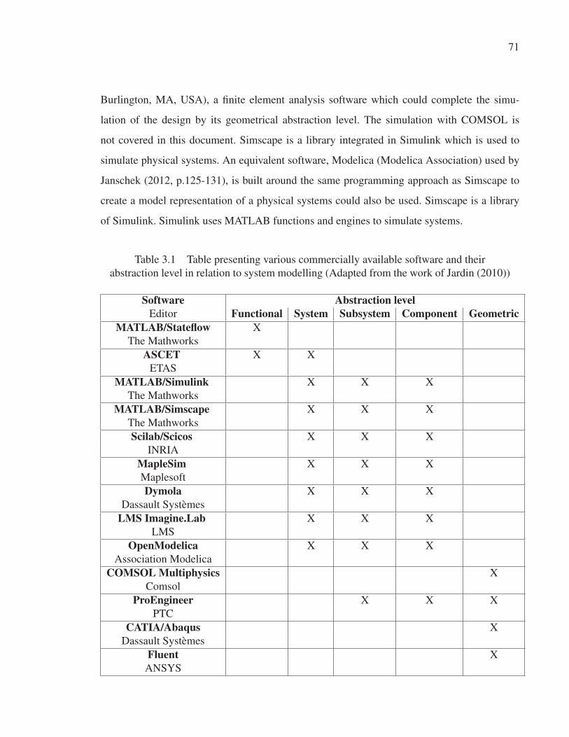
71
Burlington, MA, USA), a finite element analysis software which could complete the simu-
lation of the design by its geometrical abstraction level. The simulation with COMSOL is
not covered in this document. Simscape is a library integrated in Simulink which is used to
simulate physical systems. An equivalent software, Modelica (Modelica Association) used by
Janschek (2012, p.125-131), is built around the same programming approach as Simscape to
create a model representation of a physical systems could also be used. Simscape is a library
of Simulink. Simulink uses MATLAB functions and engines to simulate systems.
Table 3.1 Table presenting various commercially available software and their
abstraction level in relation to system modelling (Adapted from the work of Jardin (2010))
Software Abstraction levelEditor Functional System Subsystem Component Geometric
MATLAB/Stateflow X
The Mathworks
ASCET X X
ETAS
MATLAB/Simulink X X X
The Mathworks
MATLAB/Simscape X X X
The Mathworks
Scilab/Scicos X X X
INRIA
MapleSim X X X
Maplesoft
Dymola X X X
Dassault Systèmes
LMS Imagine.Lab X X X
LMS
OpenModelica X X X
Association Modelica
COMSOL Multiphysics X
Comsol
ProEngineer X X X
PTC
CATIA/Abaqus X
Dassault Systèmes
Fluent X
ANSYS

72
3.1 Fundamentals of electro-acoustic modelling
Modelling of a physical component is based on the correct definition of the quantity Across
and Through and the resulting conjugate Power. The differential in the Across quantity, called
drop, induce a Through quantity, called flow, that moves in the opposite direction of the Across
quantity to compensate the differential, as presented in Figure 3.1. The Through value can also
be the driving quantity. If so, the flow will induce a drop. The physical meaning of the measured
component is dependent of the way the Across and Through quantities are chosen as explained
by Beranek (1993, p.49). If one of the two Power variables is a very small value, that is, the
power transferred from one subsystem to the other is approximately zero, then this model will
use a single interface variable that is called a Signal and the model is so-called Signal-coupled.
Janschek (2012, p.90) uses Effort instead of Drop for the Across quantity between two points
of analysis. Effort is also linked to a human action and can also refer to an applied force. To
avoid ambiguity, the term Drop will be used to describe the Across quantity and Flow will be
used to describe the Through quantity. In Figure 3.1, the drop in acoustics is the pressure p and
the quantity going through, the flow, U in acoustics.
Figure 3.1 Conceptual view of signal Acrossand Through of a physical component in
schematic representation.
3.1.1 Impedance of physical quantities
An impedance opposes the flow when a drop is applied. If the drop is applied in a constant way,
the flow restriction - or resistance - is proportional and constant. The power necessary to create

73
this specific flow is constant too. If the drop is applied on an alternating basis, at a specific rate
per second - the frequency - the resistance is no longer constant because of the release of the
drop at each cycle. When an alternating drop is applied and released, the component impedes
the flow in a reactive way. This reactance is of an accumulative nature. It either accumulates
the drop or the flow, as explained in section 3.1.2. When the reactance is combined to the
resistance, it is called an impedance. This relation is presented in equation 3.1.
Z =dr
f(3.1)
The impedance is defined as the complex ratio between the Across quantity (dr) and Through
quantity (f ). As previously mentioned, the impedance of physical quantities, when explored in
the frequency domain, gives valuable information to understand the response of a system to a
specified stimulus, as explained in section 2.2.1.
The frequency response function is of interest for a linear time-invariant (LTI) system. A time-
invariant system is defined as a system whose output is not explicitly dependant on time. The
coefficient of transformation α, β and γ, representing the value of the components in the system
for the various physical domains, do not vary for the studied period. By definition, linearity is
the characteristic of a system f satisfying for any superposition of two input signals x1(t), x2(t)
and scalable for a constant κ:
f (x1(t) + x2(t)) = f (x1(t)) + f (x2(t))
κf (x1(t)) = f (κx1(t))(3.2)
For example, the stiffness of a loudspeaker’s suspension, when studied in its linear region, will
produce an opposite force that is proportional to the exterior force applied to it by the voice-
coil. In the large displacement region, this approximation does not hold, as discussed in section
3.2.3 and distortion occurs, as presented in section 2.2.2.

74
3.1.2 Physical analogy of components by domain
This section is inspired by a combination of the work of Beranek (1993, p.47-69) and Janschek
(2012, p.92-97). It describes the physical quantities and their equivalent in other physical do-
mains in reference to the flow f and the drop dr in the time domain. Let us consider three
proportionality constants: α, β and γ. By definition, a power consumer, or load, is described as
affected by a proportionality constant α if:
dr(t) = αf(t) (3.3)
While a flow accumulator can be analysed for the two quantities:
f(t) = βd
dtdr(t) or dr(t) = dr(t0) +
1
β
∫ t
t0
f(τ)dτ (3.4)
And the drop accumulator is:
dr(t) = γd
dtf(t) or f(t) = f(t0) +
1
γ
∫ t
t0
dr(τ)dτ (3.5)
The specific quantities of α, β and γ for the various physical domains are in Table 3.2 and the
components specificities are listed as follows:
• Mechanical Resistance displaces in direct proportionality to the sum of forces
applied to it;
• Mechanical Mass accelerates, either linearly or angularly, in direct proportionality to
the sum of forces applied to it;
• Mechanical Compliance has a velocity in direct proportionality to the sum of forces
applied to it;
• Electrical Resistance is a component which opposes to the passing current
by dissipation;

75
• Electrical Capacitance is the ability of a component to store an electrical charge as a
result of a difference in voltage;
• Electrical Inductance is a conductor which generates a magnetic field when a current
passes through it;
• Acoustical Resistor induces dissipative losses linked with a viscous movement of a
quantity of gas going through an acoustical component;
• Acoustical Compliance is a volume of air compressed by the sum of forces applied to it
without an appreciable displacement of its center of gravity;
• Acoustical Mass is a mass of air displaced by a sum of forces applied to it without
appreciably compressing it.
Table 3.2 Table of the analogy between electrical, mechanical and
acoustical quantities
Element Mechanical Electrical Acoustical
Power consumer [α] Resistance
[N s
m
]Resistor [Ω] Resistor
[N s
m5
]Flow accumulator [β] Mass [kg] Capacitor [F] Mass
[kg
m4
]Drop accumulator [γ] Compliance
[m
N
]Inductance [H] Compliance
[m5
N
]
The analogy between across and through quantities in the electrical, mechanical and acoustical
domain is presented in Table 3.3. These three domains are those that are typically found in an
earphone.
3.2 Modelling earphone-ear system coupling
Various modelling methods exist and Janschek (2012, p.90) comprehensively covers them. He
suggests five requirements to verify if a modular dynamic model is usable for computational
simulation (p.119):
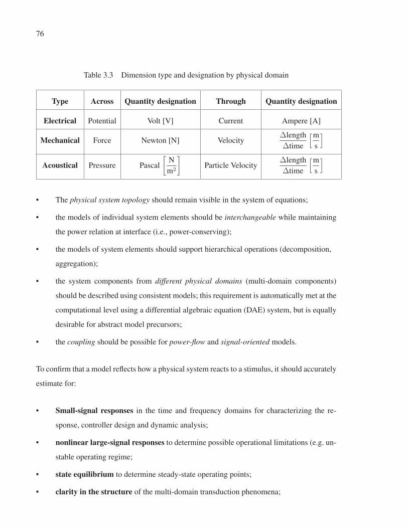
76
Table 3.3 Dimension type and designation by physical domain
Type Across Quantity designation Through Quantity designation
Electrical Potential Volt [V] Current Ampere [A]
Mechanical Force Newton [N] VelocityΔlength
Δtime
[m
s
]Acoustical Pressure Pascal
[N
m2
]Particle Velocity
Δlength
Δtime
[m
s
]
• The physical system topology should remain visible in the system of equations;
• the models of individual system elements should be interchangeable while maintaining
the power relation at interface (i.e., power-conserving);
• the models of system elements should support hierarchical operations (decomposition,
aggregation);
• the system components from different physical domains (multi-domain components)
should be described using consistent models; this requirement is automatically met at the
computational level using a differential algebraic equation (DAE) system, but is equally
desirable for abstract model precursors;
• the coupling should be possible for power-flow and signal-oriented models.
To confirm that a model reflects how a physical system reacts to a stimulus, it should accurately
estimate for:
• Small-signal responses in the time and frequency domains for characterizing the re-
sponse, controller design and dynamic analysis;
• nonlinear large-signal responses to determine possible operational limitations (e.g. un-
stable operating regime;
• state equilibrium to determine steady-state operating points;
• clarity in the structure of the multi-domain transduction phenomena;
77
• clear assignments of physical and implementation parameters to model parameters.
The models presented in this thesis are analyzed with these criteria to establish how many are
met and, therefore, how reliable the model is.
3.2.1 Common methods used to describe physical systems
Three methods are presented. They were extensively used in the literature to describe electro-
acoustical systems and the outer-ear: the lumped-element, control system block diagram and
the two-port method. Janschek (2012, p.102) briefly discussed the application of the bond
graph as a modelling tool for multi-port systems and Jardin (2010, p.198-201) covers an ap-
plication of this method to describe a moving-coil loudspeaker. Even if the main advantage of
this method is the ability to describe the domain neutral bi-directional flow of energy, some-
thing of interest for acoustically-related systems designers, this method is not covered in this
section because of the very limited literature related to it for electro-acoustic systems. Table
3.4 lists different modelling methods, and details how accurate and how reliable they are. A
section based on Control System Block Diagram is not included in the original table and has
been added.
3.2.1.1 Control System Block Diagram modelling method
A Control System Block Diagram describes the qualitative behaviour of a system and its inter-
connection within a functional model where an input data is transformed into its output using
predefined rules. It can be done in continuous time, Laplace, or discrete time domain. It is
a visual representation of the differential algebraic equations and state space equations. It is
very flexible depending on need and preferences. It can include non-linearity blocks as well as
mathematical operations and user defined functions. On the one hand, it is the most complete
and flexible modelling method, but on the other hand, it is usually more complex to use. In this
respect, it means that the control system block diagram is the modelling method that covers the
most abstraction levels. However it does not take into account the geometrical topology of the

78
Table 3.4 Table of the relationship between modelling methods
[Adapted from Mapes-Riordan (1993)]
Achievable Computational Effect of
Model Applicability accuracy complexity geometry
Lumped-parameter kL << 1 Least Least Dimensionless
method ka << 1
Transmission-line 0 < kL < ∞ Intermediate Intermediate One-dimensional
element method ka < 1.84
Control System Variable Good Intermediate One-dimensional
Block Diagram Variable
Finite-element 0 < kL < ∞ Better Most Three-dimensional
method 0 < ka < ∞
components, it only describes their behaviour. The simplest time domain output is given by:
y(t) = x(t) ∗ g(t) (3.6)
Which is represented in the block diagram as:
Figure 3.2 Control system type block diagram
representing the temporal input and output.
Then, by applying the appropriate methods, the Control System Block Diagram can be ex-
panded, reduced and modified as described by Bolton (2011) and Nise (2011). All the blocks
needed to create a Control System Block Diagram are available in the main Simulink library.
See Karris (2009) who covers several aspects of the implementation of physical components

79
in MATLAB/Simulink such as the state-space implementation and the lumped-element repre-
sentation in the time domain.
3.2.1.2 Port modelling method
Figure 3.3 Illustration of lumped networks components (terminals and ports).
[reproduced with permissions from Janschek (2012, p.90)]
A physical component can be investigated as a sub-system with two or more terminals, which
in turn can be grouped into port components, as presented in Figure 3.3. (Janschek, 2012, p.89)
describes all port components as "spatially and functionally delineated elements [which] can
mutually exchange energy with other coupled elements (the network) via interfaces (terminals
or ports)".
A one-port component is also known as a branch. A branch is a simple path composed of
a single device. By definition, the component is lumped into a geometrically dimensionless
descriptor and the relation between the branch across and branch through quantities is the
branch impedance value. The resulting product is the conjugate power handled by the branch
component. A network built out of one-port lumped-elements is connected together by lossless
connections. For a comprehensive review of the lumped-element analysis method, see Agarwal
and Lang (2005) and Lenk et al. (2011).
A Two-port network describes the relation between four quantities, two across quantities (AC)
and two through quantities (TR), linked together by a set of four transmission parameters,
A, B, C and D. Other sets of parameters exist for the transformation purpose as covered by
Attia (1999), namely z- to describe the open-circuit impedance, y- short-circuit admittance, h-

80
hybrid parameters containing open-circuit parameters (TR1 = 0) and short-circuit parameters
(AC2 = 0) and g- the inverse of the h- parameters.
Figure 3.4 Illustration of a two-port component.
⎡⎣AC1
TR1
⎤⎦ =
⎡⎣A B
C D
⎤⎦×⎡⎣AC2
TR2
⎤⎦ (3.7)
Where A and D are unitless ratios
A =AC1
AC2
∣∣∣∣TR2=0
D =TR1
TR2
∣∣∣∣AC2=0
(3.8)
While B is an impedance and C is an admittance
B =AC1
TR2
∣∣∣∣AC2=0
C =TR1
AC2
∣∣∣∣TR2=0
(3.9)
A system is considered causal when a system output y(t), as presented in Figure 3.2, is at any
time tn only affected by the input x(t) up to time tn. So any description method presenting a
direct relation between the input and output of a system is causal. For Janschek (2012, p.118),
"it should be pointed out again that the advantages of multi-port physical modeling come from
its equation-oriented description with indeterminate causal structure, and not, mistakenly, from
acausal models".
In earphones, cascade association of two-port as well as parallel association can be consid-
ered. The computation of the cascade and parallel features are performed using the derived
Kirchoff’s law applied to fluid flow by using the analogies described in Table 3.3. The physical

81
elements transfer the mass from one element (k) to another (l) at the junction between them.
As stated above, the elements can be defined by a generic two-port representation:
[a]k =
⎡⎣Ak Bk
Ck Dk
⎤⎦ [a]l =
⎡⎣Al Bl
Cl Dl
⎤⎦ (3.10)
Upon inspection, the following relation can be found when in cascade as presented in Figure
3.5:
Figure 3.5 Cascade of a two-port network presented with the across and
through quantities.
⎧⎨⎩AkCin �= Ak
C1
T kRin = T k
R1
⎫⎬⎭⎧⎨⎩Ak
C1 = AlC2
T kR1 = T l
R2
⎫⎬⎭⎧⎨⎩Al
C2 �= AlCout
T lR2 = T l
Rout
⎫⎬⎭⇒⎧⎨⎩Al
Cin �= AkCout
T lRin = T k
Rout
⎫⎬⎭ (3.11)
And the equivalent transmission line matrix of element k combined to element l is given by:
[a]k ∗ [a]l =⎡⎣Ak Bk
Ck Dk
⎤⎦ ∗⎡⎣Al Bl
Cl Dl
⎤⎦ =
⎡⎣AkAl +BkCl AkBl +BkDl
CkAl + ClDk BlCk +DkDl
⎤⎦ (3.12)
When the same matrices are in parallel to each other, again, the relation is:⎧⎨⎩ACin = AkCin = Al
Cin
TRin = T kRin + T l
Rin
⎫⎬⎭⎧⎨⎩ACout = Ak
Cout = AlCout
TRout = T kRout + T l
Rout
⎫⎬⎭⇒⎧⎨⎩Ak
Cin = AlCin �= Al
Cout = AkCout
TRin = TRout �= T kR �= T l
R
⎫⎬⎭(3.13)

82
Figure 3.6 Parallel of a two-port network presented with the across and
through quantities.
[a]k ‖ [a]l =
⎡⎣Ak Bk
Ck Dk
⎤⎦ ‖⎡⎣Al Bl
Cl Dl
⎤⎦ =
⎡⎢⎣AkBl + AlBk
Bk +Bl
BkBl
Bk +Bl
Ck + Cl(Al − Ak) (Dk −Dl)
Bk +Bl
DkBl +DlBk
Bk +Bl
⎤⎥⎦(3.14)
3.2.2 Models of a human ear
The couplers that simulate the average human ear are presented in Table 2.1 of section 2.2. A
sectional view of the IEC 60318-4 coupler is presented in Figure 3.7. To simulate the couplers,
it is necessary to establish the behaviour of the components in order to reproduce the coupler as
an assembly of lumped-elements. Jønsson et al. (2004) compared the lumped-element model
provided by Brüel & Kjær (1997), presented in Figure 3.8, with a Finite Element Model (FEM).
They found a very good agreement across the entire frequency range where it is expected,
validating the lumped-element model. The coefficients of each lumped-element are presented
in Table 3.5.
An alternate model is to approximate the ear by the equivalent compliance of a close volume of
2 cm3. The equivalent compliance is 1.4049 × 10⁻¹¹[
m5
N
]. The details of this calculation can
be found in Appendix IV. The model approximated by an equivalent compliance is of limited
application because of the limitation of the lumped-element method as shown in Table 3.4.
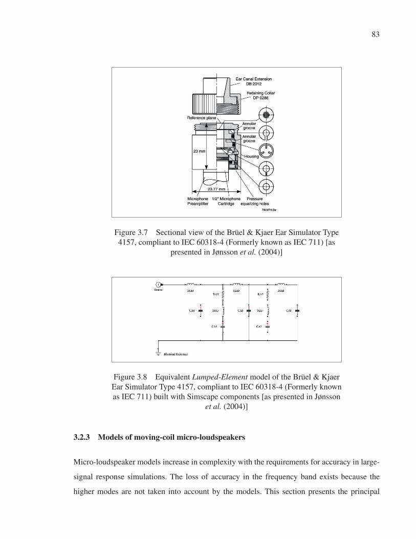
83
Figure 3.7 Sectional view of the Brüel & Kjaer Ear Simulator Type
4157, compliant to IEC 60318-4 (Formerly known as IEC 711) [as
presented in Jønsson et al. (2004)]
Figure 3.8 Equivalent Lumped-Element model of the Brüel & Kjaer
Ear Simulator Type 4157, compliant to IEC 60318-4 (Formerly known
as IEC 711) built with Simscape components [as presented in Jønsson
et al. (2004)]
3.2.3 Models of moving-coil micro-loudspeakers
Micro-loudspeaker models increase in complexity with the requirements for accuracy in large-
signal response simulations. The loss of accuracy in the frequency band exists because the
higher modes are not taken into account by the models. This section presents the principal
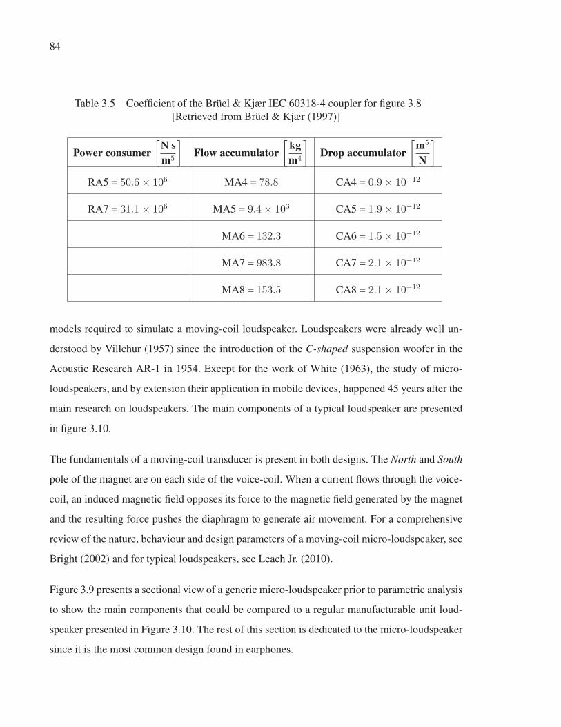
84
Table 3.5 Coefficient of the Brüel & Kjær IEC 60318-4 coupler for figure 3.8
[Retrieved from Brüel & Kjær (1997)]
Power consumer[
N sm5
]Flow accumulator
[kgm4
]Drop accumulator
[m5
N
]RA5 = 50.6× 10⁶ MA4 = 78.8 CA4 = 0.9× 10⁻¹²
RA7 = 31.1× 10⁶ MA5 = 9.4× 10³ CA5 = 1.9× 10⁻¹²
MA6 = 132.3 CA6 = 1.5× 10⁻¹²
MA7 = 983.8 CA7 = 2.1× 10⁻¹²
MA8 = 153.5 CA8 = 2.1× 10⁻¹²
models required to simulate a moving-coil loudspeaker. Loudspeakers were already well un-
derstood by Villchur (1957) since the introduction of the C-shaped suspension woofer in the
Acoustic Research AR-1 in 1954. Except for the work of White (1963), the study of micro-
loudspeakers, and by extension their application in mobile devices, happened 45 years after the
main research on loudspeakers. The main components of a typical loudspeaker are presented
in figure 3.10.
The fundamentals of a moving-coil transducer is present in both designs. The North and South
pole of the magnet are on each side of the voice-coil. When a current flows through the voice-
coil, an induced magnetic field opposes its force to the magnetic field generated by the magnet
and the resulting force pushes the diaphragm to generate air movement. For a comprehensive
review of the nature, behaviour and design parameters of a moving-coil micro-loudspeaker, see
Bright (2002) and for typical loudspeakers, see Leach Jr. (2010).
Figure 3.9 presents a sectional view of a generic micro-loudspeaker prior to parametric analysis
to show the main components that could be compared to a regular manufacturable unit loud-
speaker presented in Figure 3.10. The rest of this section is dedicated to the micro-loudspeaker
since it is the most common design found in earphones.
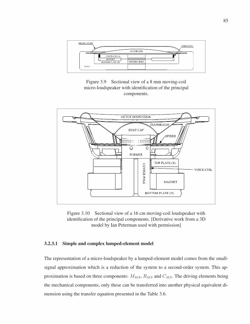
85
Figure 3.9 Sectional view of a 8 mm moving-coil
micro-loudspeaker with identification of the principal
components.
Figure 3.10 Sectional view of a 16 cm moving-coil loudspeaker with
identification of the principal components. [Derivative work from a 3D
model by Ian Peterman used with permission]
3.2.3.1 Simple and complex lumped-element model
The representation of a micro-loudspeaker by a lumped-element model comes from the small-
signal approximation which is a reduction of the system to a second-order system. This ap-
proximation is based on three components: MMS , RMS and CMS . The driving elements being
the mechanical components, only these can be transferred into another physical equivalent di-
mension using the transfer equation presented in the Table 3.6.

86
Figure 3.11 Equivalent lumped-element network for the discrete
components of a loudspeaker, A) Mechanical abstraction, B) Mechanical
equivalent network, C) Electrical equivalent network, D) Acoustical
equivalent network.
In the models presented in figure 3.11, ideal transformers are used. An ideal transformer is used
to link a physical domain to another. It is a lossless transformation of the across in one domain
to the through in another domain. The transformation relation of ϑ : 1 for across quantities AC1
and AC2 and their relative quantities TR1 and TR2 is given by equation:
ϑAC1 = AC2 andTR1
ϑ= TR2 (3.15)
While the three main elements are sufficient to achieve a low-frequencies approximation of the
response of the driver - up to the first resonance - in the stiffness controlled section, the part
controlled by the voice-coil inductance losses is not taken into account. The lossy voice-coil

87
Table 3.6 Table of the analogy between electrical, mechanical and
acoustical quantities
Element Mechanical Electrical Acoustical
Power consumer RMS
[kg
s
]RES =
(Bl)2
RMS
[Ω] RAS =RMS
S2d
[Ωa]
Flow accumulator MMS [kg] CES =MMS
(Bl)2[F] MAS =
MMS
S2d
[kg
m4
]Drop accumulator CMS
[m
N
]LES = CES(Bl)2[H] CAS = CMSS
2d
[m3
Pa
]
inductance is explained by Leach Jr. (2010, p.106) and can be added to the model to achieve
greater accuracy. The computation of LE and RE is covered in section 2.1.
3.2.3.2 Two-Port model
A two-port model of a loudspeaker is presented by Darlington (1998) as:
⎡⎣A B
C D
⎤⎦ =
⎡⎢⎣ZEBSD
Bl
ZMZEB + (Bl)2
BlS
Bl
ZM
Bl
⎤⎥⎦ (3.16)
In the equation 3.16, the parameters are the same as the lumped-element model. ZM is the me-
chanical impedance in[Nsm
]and ZEB is the blocked electrical impedance in [Ω]. The MATLAB
code for the two-port application is presented in Appendix II.
3.2.3.3 Block-diagram model
The complex block-diagram model, which includes nonlinearities, as presented by Sturtzer
et al. (2012) is reproduced hereafter. The current-driven model is presented in Fig. 3.12 while
the voltage-driven model is presented in Fig. 3.13. When the quality of the acoustical output
of a micro-loudspeaker is not considered in a model, the micro-loudspeaker is fundamentally a
generic loaded mechatronic transducer as defined by Janschek (2012, p.311-349). Sturtzer et al.
(2012) uses polynomial coefficients to express the relationships between diaphragm excursion

88
and other variables dependent on membrane excursion. The polynomial regression used is a
relationship between the independent relation, excursion and a dependent variable, in this case
CM(x), Bl(x) and LE(x). The general representation of a polynomial regression for a system
f is:
f(x) = a0 + a1(x) + a2(x)2 + . . .+ an(x)
n + ε (3.17)
where every coefficient an is determined experimentally and the error ε is a factor of N(0, σ2),
the difference between the measured value and the estimated value of the regression.
Figure 3.12 Current driven micro-speaker block diagram.
[As presented in Sturtzer et al. (2012)]
By applying the regression approach for the excursion x as the independent variable, Sturtzer
et al. (2012) gave three nonlinear approximations by using these regressions:
CM(x) = CM0 +n∑
n=1
(CMnxn)
Bl(x) = Bl0 +n∑
n=1
(Blnxn)
LE(x) = LE0 +n∑
n=1
(LEnxn)
(3.18)

89
Equation 3.18 can be computed using typical measurements. Comparison of Figure 3.12 and
Figure 3.13 LE(x) is absent from the current driven loudspeaker model. This is because, as
presented in equation 3.5 and table 3.2, the voice-coil is current driven by definition.
Figure 3.13 Voltage driven micro-speaker block diagram.
[As presented in Sturtzer et al. (2012)]
The block diagram model is more complete, but also more complex. Each model can comple-
ment each other by either offering speed or more reliable results. For example, the lumped-
element implementation provides a quick first approximation of the frequency response of a
moving-coil micro-loudspeaker earphone while a control system block diagram would require
more measurements but would yield a more accurate result.
3.2.4 Models of balanced-armature micro-loudspeakers
Jensen (2009) describes a balanced-armature loudspeaker as presented in figure 3.14 as fol-
lows:
An armature is balanced in the magnetic field between two permanent magnets.
The armature (the piece of metal in the air gap between the magnets) is balanced in
the sense that both permanent magnets exert an equal but opposite magnetic force

90
on the armature when the electrical current in the coil is zero. The armature itself
is not a very efficient sound radiator so the armature is rigidly connected to a thin
and light diaphragm, where the front and back of the diaphragm are acoustically
isolated.
Figure 3.14 A sectional view of a Knowles Electronic EH
balanced-armature loudspeaker. [Reproduced with permission from
Knowles Electronics, Itasca, IL.]
For a complete description of the interaction between each of the domains included in a
balanced-armature receiver, see Jensen (2009) and Vitt (2011).
3.2.4.1 Lumped-elements models
Balanced-armature lumped-elements models are constructed using the same approach as the
moving-coil micro-loudspeaker. Table 3.4 presents the equivalent quantities to use for model
construction. The presence of gyrators in the model is to be noted. A gyrator is a lossless
component that relates two sets of across and through by a constant factor. In a gyrator, the
quantity across in one domain is proportional to the quantity through in the other domain.
In figure 3.15, the model presents the aggregation between the same domains as for the moving-
coil loudspeaker, namely electrical to mechanical via a magnetic field and from mechanical to
acoustical with a membrane. This relationship depends on the distance between the armature
and the magnet. As presented by Jensen (2009, p.19), the reluctance of the air gap is considered

91
Figure 3.15 Balanced-armature micro-speaker lumped-element model.
[Reproduced with permission from Knowles Electronics, Itasca, IL.]
to be much larger than the reluctance of the core and the magnet. Therefore, changing the
position of the armature and reducing the air gap will change the reluctance.
3.2.4.2 Complex control system block-diagram model
As stated above, the position of a balanced-armature loudspeaker is dependant on its position,
but also on the variation of the position within the air gap. The variation of the air gap is an in-
dependent variable of a moving-coil loudspeaker since it moves axially and not radially. These
relationships, explicitly presented by Jensen (2009), are converted into a Simulink control sys-
tem block diagram in figure 3.16. The input is a current and the output is either a position,
a velocity or an acceleration of the armature. The sound pressure generated by the unit in a
known volume is a function of the position, the surface of the diagram and the specific acoustic
compliance |p| = CASD|x|.
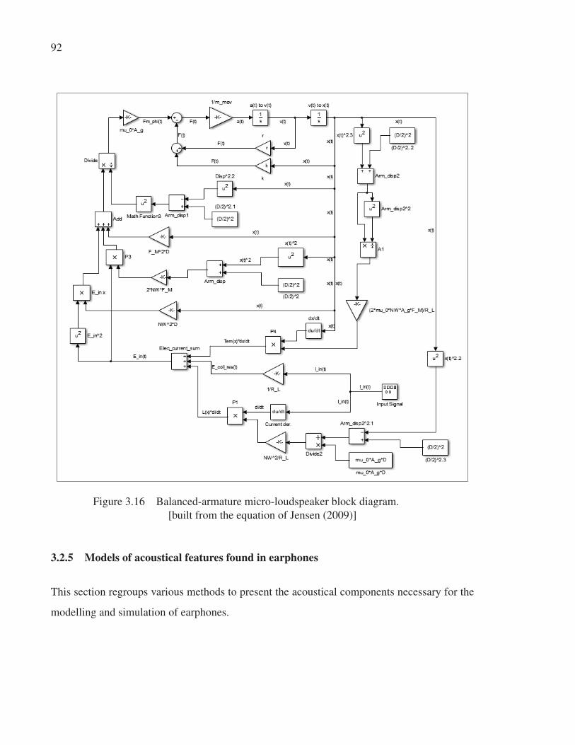
92
Figure 3.16 Balanced-armature micro-loudspeaker block diagram.
[built from the equation of Jensen (2009)]
3.2.5 Models of acoustical features found in earphones
This section regroups various methods to present the acoustical components necessary for the
modelling and simulation of earphones.
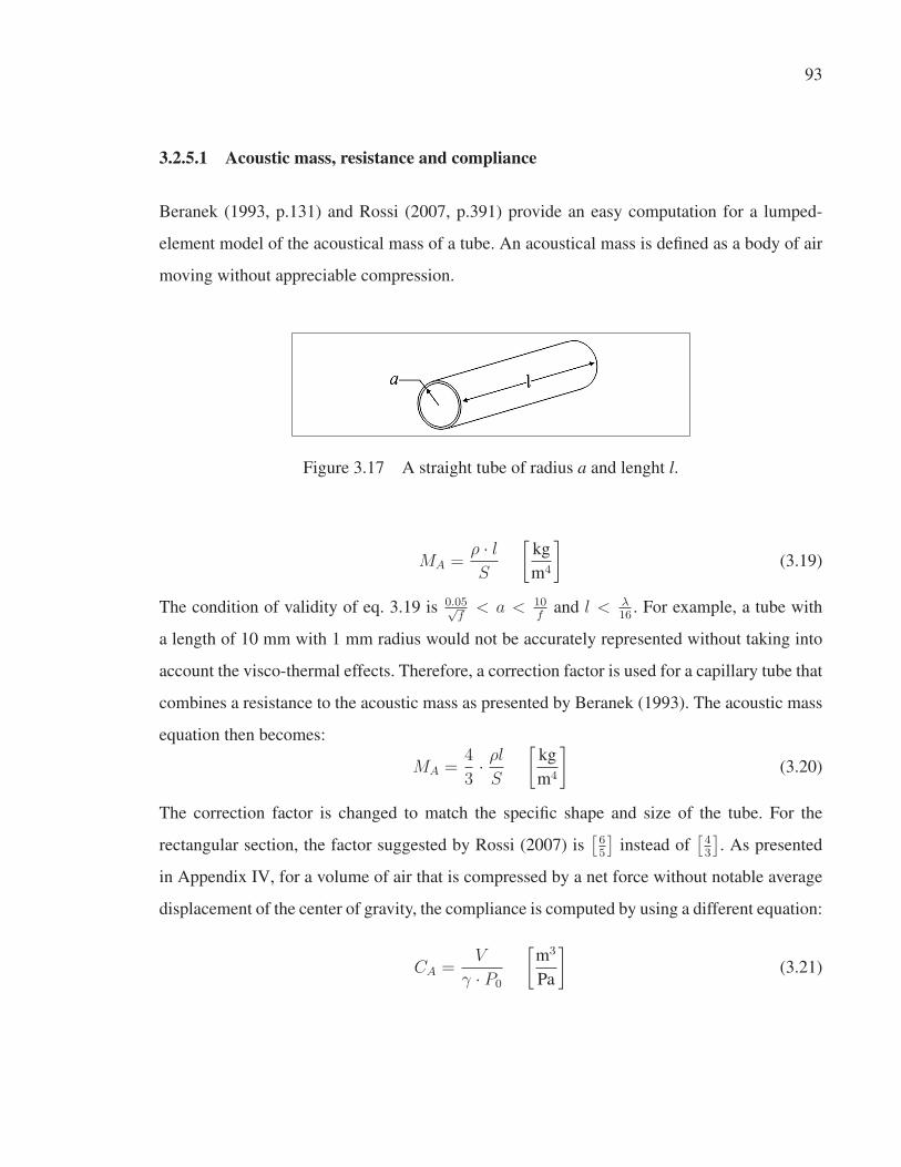
93
3.2.5.1 Acoustic mass, resistance and compliance
Beranek (1993, p.131) and Rossi (2007, p.391) provide an easy computation for a lumped-
element model of the acoustical mass of a tube. An acoustical mass is defined as a body of air
moving without appreciable compression.
Figure 3.17 A straight tube of radius a and lenght l.
MA =ρ · lS
[kg
m4
](3.19)
The condition of validity of eq. 3.19 is 0.05√f
< a < 10f
and l < λ16
. For example, a tube with
a length of 10 mm with 1 mm radius would not be accurately represented without taking into
account the visco-thermal effects. Therefore, a correction factor is used for a capillary tube that
combines a resistance to the acoustic mass as presented by Beranek (1993). The acoustic mass
equation then becomes:
MA =4
3· ρlS
[kg
m4
](3.20)
The correction factor is changed to match the specific shape and size of the tube. For the
rectangular section, the factor suggested by Rossi (2007) is[65
]instead of
[43
]. As presented
in Appendix IV, for a volume of air that is compressed by a net force without notable average
displacement of the center of gravity, the compliance is computed by using a different equation:
CA =V
γ · P0
[m3
Pa
](3.21)

94
A model of the propagation of sound waves in tubes using a two-port approach is presented by
Egolf et al. (1978) for a tube of lenght ln and radius an:
⎡⎣An Bn
Cn Dn
⎤⎦ =
⎡⎣ coshΓnln ZnsinhΓnln
Z−1n sinhΓnln coshΓnln
⎤⎦ (3.22)
Where Γn is the propagation operator of tube n
Γn = ıω
c
⎧⎨⎩1 + 2(γ − 1)[
[J1(αanαanJ0αan
]1− 2J1(βan)
βanJ0(βan)
⎫⎬⎭12
(3.23)
and Zn is the caracteristic impedance of tube n
Zn =ρc
πa2n
{[1− 2J1βan
βanJ0(βan)
] [1 + 2(γ − 1)
J1(αanαanJ0(αan
]}− 12
(3.24)
while α =(
−ıωρσμ
) 12
and β =(
−ıωρμ
) 12
This two-port model is applicable for acoustic mass as well as acoustical compliance since it
takes into account the wave behaviour within the component. A similar way to compute the
two-port model of a small tube including visco-thermal effects, is presented in Keefe (1984).
This equation is reused by Mapes-Riordan (1993) to describe transmission-line elements of
horns. He offers a simpler definition of Γn and Zn
Γn = k
⎡⎣⎛⎝1.045
(√ρωS
ηπ
)−1⎞⎠+ ı
⎛⎝1.045
(√ρωS
ηπ
)−1⎞⎠⎤⎦ (3.25)
Zn =ρc
S
⎡⎣⎛⎝1 + 0.369
(√ρωS
ηπ
)−1⎞⎠−1
−⎛⎝ı0.369
(√ρωS
ηπ
)−1⎞⎠⎤⎦ (3.26)
An alternate model from Zuercher et al. (1988) helps simplify the computation. This is a FOR-
TRAN based approximation program which accelerates the process compared to the Bessel
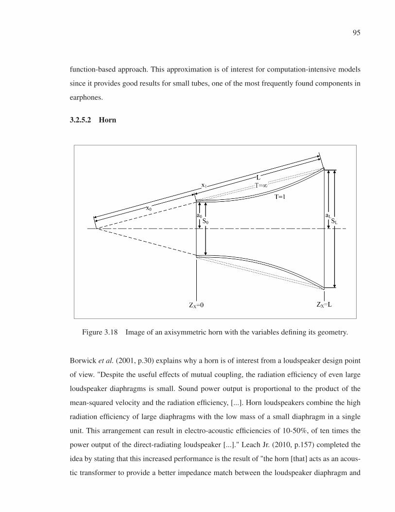
95
function-based approach. This approximation is of interest for computation-intensive models
since it provides good results for small tubes, one of the most frequently found components in
earphones.
3.2.5.2 Horn
Figure 3.18 Image of an axisymmetric horn with the variables defining its geometry.
Borwick et al. (2001, p.30) explains why a horn is of interest from a loudspeaker design point
of view. "Despite the useful effects of mutual coupling, the radiation efficiency of even large
loudspeaker diaphragms is small. Sound power output is proportional to the product of the
mean-squared velocity and the radiation efficiency, [...]. Horn loudspeakers combine the high
radiation efficiency of large diaphragms with the low mass of a small diaphragm in a single
unit. This arrangement can result in electro-acoustic efficiencies of 10-50%, of ten times the
power output of the direct-radiating loudspeaker [...]." Leach Jr. (2010, p.157) completed the
idea by stating that this increased performance is the result of "the horn [that] acts as an acous-
tic transformer to provide a better impedance match between the loudspeaker diaphragm and

96
the load." Many horn configurations exist but only axisymmetric ones are presented here. The
model of Mapes-Riordan (1993) simulates the model of Webster and Salmon (1944), as pre-
sented in Post (1994) and Leach Jr. (2010, 157-174). The curvature of the walls of the horn
are dependent on the factor T which provides the shape of the horn. Detailed variations of the
possible shapes of an axisymmetric horn are presented in Leach Jr. (2010, 157-174). Mapes-
Riordan (1993) offer a model of a conical lossless horn in a two-port configuration:
A =
(x1
x0
)cos(kL)−
(1
kx0
)sin(kL)
B =
(x0
x1
)jR0sin(kL)
C =
(j
R0
)[(x1
x0
(1
kx0
)2)sin(kL)−
(L
x0
)(1
kx0
)cos(kL)
]
D =
(x0
x1
)(cos(kL) +
(1
kx0
sin(kL)
))(3.27)
And a dissipative two-port option:
A =
(x1
x0
)[cosh(ΓL)−
(1
Γx1
)sinh(ΓL)
]B =
(x0
x1
)Zcsinh(ΓL)
C =
(1
Zc
)(x1
x0
−(
1
Γx0
)2)sinh(ΓL) +
(ΓL
(Γx0)2
)cosh(ΓL)
D =
(x0
x1
)[cosh(ΓL)−
(1
Γx0
)sinh(ΓL)
](3.28)
For certain applications where the horn is much larger than the wavelength, the lossless ver-
sion, which only expresses the flow and drop accumulator behaviours, yields a good result
because the loss is not significant. For applications such as earphones, the loss from the small
components becomes important enough that it needs to be taken into account.

97
3.2.5.3 Sudden section change
When a sudden section change occurs, as presented in Figure 3.19, the pressure at the interface
is the same, but the flow becomes different since the space to fill is changing. This ratio of
through quantity is represented in the D coefficient of the 2× 2 matrix of a two-port represen-
tation, as explained in section 3.2.1.2. The ratio is computed in the direction of the flow: if the
S1S2
Figure 3.19 Image of a sudden change from
section S1 to section S2.
flow is coming from S1, the ratio is as presented in equation 3.29.
⎡⎣A B
C D
⎤⎦ =
⎡⎢⎣1 0
0S2
S1
⎤⎥⎦ (3.29)
If the flow is reversed, ratioS2
S1
is reversed as well.
3.2.5.4 Synthetic material membrane
Poldy (1983b) models a membrane as a second-order component equivalent to a frequency
independent RLC network in the electric analogy, as established in Table 3.2. It is the equivalent
of the lumped-elements model for a loudspeaker. The main difference is the mass of the voice-

98
Figure 3.20 Schematic of a synthetic material membrane
activated by a displacement source. [Adapted from Poldy (1983b)]
coil and former which is not present. These values are presented in Table 3.6. In practice, the
measure of the impedance of a device is performed by using a tool as presented in Figure 3.21.
The left and right sides of the tubes are modelled as two-ports of a one-dimensional acoustic
tube using equation 3.22. The adjustment piston is used to change the standing wave frequency
dependent on the length of the tube, to be able to measure the material under test for any
frequency and achieve a more reliable model.
Figure 3.21 Schematic of a measurement apparatus used to measure membranes and
porous material [Adapted from Poldy (1983b)]
As presented in equation 3.9, the impedance of a system is represented by the B coefficient of
the 2 × 2 matrix of a two-port representation. For a very thin and non-porous membrane, it is
assumed that volume velocity behind and in front of the membrane is the same, leaving the A

99
factor to 1, leaving C = 0 and D = 1.
⎡⎣A B
C D
⎤⎦ =
⎡⎣1 Zm
0 1
⎤⎦ (3.30)
The approximation for a membrane without air flowing through is given by equation 3.31
where values Rm, Lm and Cm are mechanical quantities as defined in Table 3.2:
Zm = Rm + ıωLm
(1− 1
ıωCm
)(3.31)
A complete two-port model can be obtained by measuring both pressure and particle velocity
on either side of the membrane that is to be used in a specific design. The pressure must be
measured using four microphones as presented in Figure 3.21 to successfully measure particle
velocity as well as the pressure. Measurement of the particle velocity ul variation is possible
by the differential in pressure amplitude Δp of a single frequency ω propagating along the tube
L at a position l. The distance between the microphones Δmicl should be much smaller than
the studied wavelength. The relation is:
ul =Δp(l)
ωρ0Δmicl(3.32)
3.2.5.5 Perforated sheets, meshes and foams
Perforated sheets, meshes and foams are known as acoustic mixed-elements. They are usu-
ally placed in cascade with other components of the acoustical path to transform the sound as
needed, to protect a fragile component such as the diaphragm, or prevent debris from penetrat-
ing into the assembly. These features have a noticeable impact on the frequency response of
the micro-loudspeaker. The method in Figure 3.21 is a way to quantify their impact.
An alternative to the measurement of the two-port network for these features is to use the
lumped-element modelling method as demonstrated by Shiah et al. (2008). They analysed a
perforated sheet which is essentially a series of acoustic masses and resistances coupled with

100
Figure 3.22 Image of a perforated sheet, as
typically found in moving-coil micro-loudspeaker
to protect the diaphragm.
a radiation impedance. They studied the shape of the front cover by using a lumped-element
approach. The acoustical resistance due to the presence of the front cover Rfc is given by
equation 3.33:
Rfc =8πμtshAfc
(3.33)
where μ is air viscosity, tsh is the plate thickness in m and Afc is the surface area of the hole.
The acoustical mass is given by equation 3.19. And Cfc uses the equation 3.21 to model the
space between the diaphragm and the front cover.
3.2.6 Limitations of the modelling and simulation methods
Models and simulations increase in reliability, as compared to a Real World Observation, when
they take into account more and more design variables. On the one hand, when an important
variable such as the stiffness of a material is quantified, it provides a more accurate model. A
model disregarding important variables is not reliable and therefore not useful. On the other
hand, including all the phenomena that are part of a physical system would be computation-
ally intensive and would not necessarily yield more reliable results because of the introduction
of uncontrollable factors. It is preferable to model and simulate only the frequency range of
interest, as it has been done in section 3.2.7, because a very accurate simulation is time and
resource consuming, so it should be proportionate to the expected outcomes. A new design
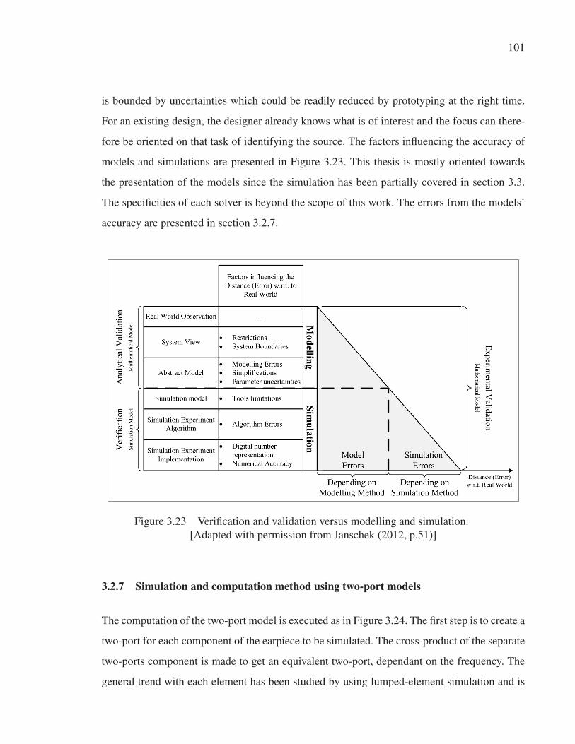
101
is bounded by uncertainties which could be readily reduced by prototyping at the right time.
For an existing design, the designer already knows what is of interest and the focus can there-
fore be oriented on that task of identifying the source. The factors influencing the accuracy of
models and simulations are presented in Figure 3.23. This thesis is mostly oriented towards
the presentation of the models since the simulation has been partially covered in section 3.3.
The specificities of each solver is beyond the scope of this work. The errors from the models’
accuracy are presented in section 3.2.7.
Figure 3.23 Verification and validation versus modelling and simulation.
[Adapted with permission from Janschek (2012, p.51)]
3.2.7 Simulation and computation method using two-port models
The computation of the two-port model is executed as in Figure 3.24. The first step is to create a
two-port for each component of the earpiece to be simulated. The cross-product of the separate
two-ports component is made to get an equivalent two-port, dependant on the frequency. The
general trend with each element has been studied by using lumped-element simulation and is
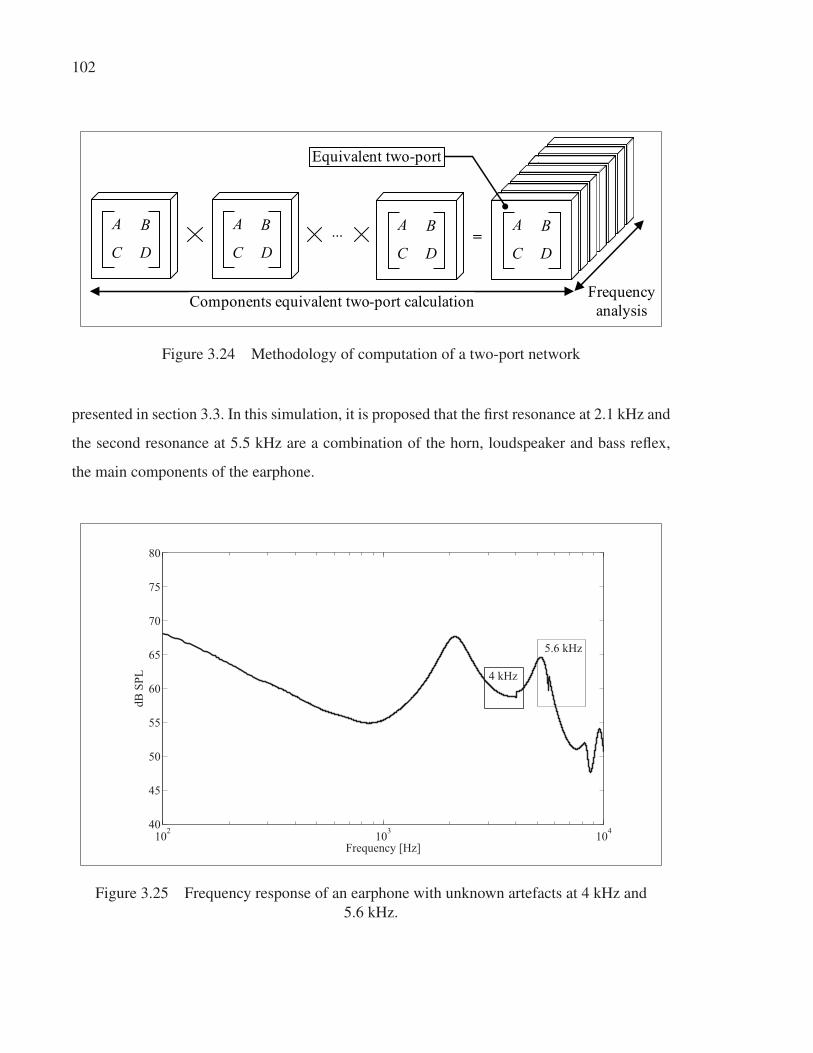
102
DC
BA
DC
BA ...DC
BA
DC
BA
Components equivalent two-port calculation Frequencyanalysis
=
Equivalent two-port
Figure 3.24 Methodology of computation of a two-port network
presented in section 3.3. In this simulation, it is proposed that the first resonance at 2.1 kHz and
the second resonance at 5.5 kHz are a combination of the horn, loudspeaker and bass reflex,
the main components of the earphone.
102 103 10440
45
50
55
60
65
70
75
80
Frequency [Hz]
dB S
PL
5.6 kHz
4 kHz
Figure 3.25 Frequency response of an earphone with unknown artefacts at 4 kHz and
5.6 kHz.

103
2 000 3000 4000 5000 6000 700040
45
50
55
60
65
70
75
80
Frequency [Hz]
dB S
PL
Two−port simulationMeasured on a IEC60318−4 coupler
5.6 kHz4 kHz
Figure 3.26 Frequency response of an earphone with artefacts at 4 kHz and 5.6 kHz due
to front tubes.
One of the purposes of using the two-port approximation is to identify small artefacts in the
frequency response, not present in the lumped-element simulation. However, no model is more
precise than its least precise component, as explained in section 3.2.6. Two of these artefacts
have been identified around 4 kHz and 5.6 kHz. By their position and amplitude on the fre-
quency response, the front section of the earpiece has been modelled by using the two-port
approximation of a tube, as in section 3.2.5. The front section is composed of two distinctive
sections, one made of silicone of a diameter of 2.5 mm by 3 mm long. The second section
is a rigid plastic section of a diameter of 3 mm by 0.7 mm long. By using the two-port ap-
proximation of a tube, it is seen that the 4 kHz artefact is present when the plastic section is
present and the 5.6 kHz artefact is present when the silicon section is present. Ultimately, the
earpiece is dedicated to sound reproduction and the decision to rework the design to eliminate
these artefacts has to be counterbalanced with the perceived effect by a subject, a topic that was
explored in Chapter 1.

104
3.3 Introduction to Design, Modelling and Simulation of Earphones with Simulink®
This section presents a journal paper submitted to the Journal of the Audio Engineering Society
by Cédrik Bacon and Jérémie Voix on June 27th, 2013.
3.3.1 Abstract
Electro-acoustic simulation is a field that implicitly requires multi-domain analysis to success-
fully integrate electrical, mechanical and acoustical phenomena from various sources, to facili-
tate and accelerate the conversion of models from heterogeneous to homogeneous. This article
proposes Simulink®, a block diagram environment for multi-domain simulation and Model-
Based Design. This software allows for heterogeneous models when simulating, which results
in more efficient and flexible implementation. Models of electro-acoustic components typically
found in insert earphones such as micro-loudspeakers models as well as components such as
tubes, cavities and average ear models are included; solver characteristics as well as coupling
between domains necessary for the simulation are also covered. Simulations of earphones with
several components are presented to demonstrate implementation.
3.3.2 Introduction
This article introduces how to use Simulink® as an electro-acoustical model simulator and more
precisely, how to implement electro-acoustic models from various sources into the software.
To the authors’ knowledge, this topic has not yet been directly covered in the literature. Several
software programs can be used to simulate electro-acoustic systems. For instance, Leach Leach
Jr. (1991) has documented how to use SPICE as a computer-aided electro-acoustic design tool.
Yet, despite being widely in-use and convenient Kahrs (2009), SPICE does not convert all mod-
els into electrical circuit equivalents. Simulink offers this possibility by enabling multi-domain
simulations and Model-Based Design. Another valuable feature is the Graphic User Interface
(GUI) that enables a new user to reuse blocks constructed by other users without having to
master all the steps needed to create them. Within Simulink, there is a library of components
called Simscape™, which provides an environment for modelling and simulating physical sys-

105
tems with their dimensions, while Simulink is by default dimensionless. This article covers
two modelling methods, Lumped-Element and Control System Block Diagram in Section 3.3.3.
It presents how to use simple acoustical components in the Lumped-Element abstraction in
Section 3.3.4 and how to reproduce the equivalent model for an occluded-ear simulator (IEC
60318-4) and a 2 cm3 coupler (IEC 60318-5) within Simscape. It also presents two types of
micro-loudspeakers, moving-coil and balanced-armature, and their description in the Lumped-
Element and Control System Block Diagram modelling methods in Section 3.3.4.3. In Section
3.3.5, particularities of the simulation are presented. Finally, the models presented in the article
are compared and the measurement of physical units is made in Section 3.3.7.
3.3.3 Description of modelling methods
The models of physical phenomenon presented in technical documentation are not presented
in a uniform way; Differential-Algebraic Equation are used for mathematical representation
while Lumped-element, and Control System Block Diagram are common representation meth-
ods found in the literature Poldy (1983a), Beranek (1993), Lenk et al. (2011). Converting one
of these representations into another representation can be tedious. Using software that uses
the models as they are presented in the original research accelerates the process and reduces
the possibility of introducing an error. This section covers these types of model representations
and how to implement them in Simulink.
3.3.3.1 Ordinary Differential Equation and Differential Algebraic Equation
Systems of differential equations that are subject to algebraic constraints are called Differential
Algebraic Equations (DAEs). A DAE without algebraic constraints is called an Index-0 DAE
or Ordinary Differential Equation (ODE). By definition, "An Ordinary Differential Equation
(ODE) is an equation that contains one or several derivatives of an unknown function, which
we usually call y(x) (or sometimes y(t) if the independent variable is time t). The equation
may also contain y itself, known functions of x (or t), and constants" Kreyszig (2010). Thus,
the application is similar for ODEs and for DAEs. However, Simulink differentiates between
DAEs and ODEs when selecting a solver because of the algebraic loop issue. It is preferable to
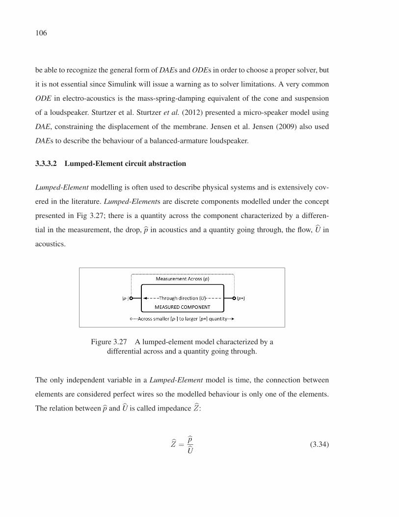
106
be able to recognize the general form of DAEs and ODEs in order to choose a proper solver, but
it is not essential since Simulink will issue a warning as to solver limitations. A very common
ODE in electro-acoustics is the mass-spring-damping equivalent of the cone and suspension
of a loudspeaker. Sturtzer et al. Sturtzer et al. (2012) presented a micro-speaker model using
DAE, constraining the displacement of the membrane. Jensen et al. Jensen (2009) also used
DAEs to describe the behaviour of a balanced-armature loudspeaker.
3.3.3.2 Lumped-Element circuit abstraction
Lumped-Element modelling is often used to describe physical systems and is extensively cov-
ered in the literature. Lumped-Elements are discrete components modelled under the concept
presented in Fig 3.27; there is a quantity across the component characterized by a differen-
tial in the measurement, the drop, p in acoustics and a quantity going through, the flow, U in
acoustics.
Figure 3.27 A lumped-element model characterized by a
differential across and a quantity going through.
The only independent variable in a Lumped-Element model is time, the connection between
elements are considered perfect wires so the modelled behaviour is only one of the elements.
The relation between p and U is called impedance Z:
Z =p
U(3.34)
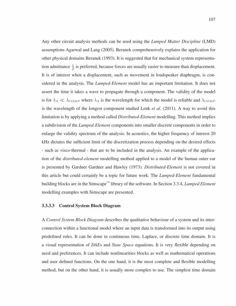
107
Any other circuit analysis methods can be used using the Lumped Matter Discipline (LMD)
assumptions Agarwal and Lang (2005). Beranek comprehensively explains the application for
other physical domains Beranek (1993). It is suggested that for mechanical system representa-
tion admittance 1
Zis preferred, because forces are usually easier to measure than displacement.
It is of interest when a displacement, such as movement in loudspeaker diaphragm, is con-
sidered in the analysis. The Lumped-Element model has an important limitation. It does not
assert the time it takes a wave to propagate through a component. The validity of the model
is for λA � λCOMP where λA is the wavelength for which the model is reliable and λCOMP
is the wavelength of the longest component studied Lenk et al. (2011). A way to avoid this
limitation is by applying a method called Distributed-Element modelling. This method implies
a subdivision of the Lumped-Element components into smaller discrete components in order to
enlarge the validity spectrum of the analysis. In acoustics, the higher frequency of interest 20
kHz dictates the sufficient limit of the discretization process depending on the desired effects
- such as visco-thermal - that are to be included in the analysis. An example of the applica-
tion of the distributed-element modelling method applied to a model of the human outer ear
is presented by Gardner Gardner and Hawley (1973). Distributed-Element is not covered in
this article but could certainly be a topic for future work. The Lumped-Element fundamental
building blocks are in the Simscape™ library of the software. In Section 3.3.4, Lumped Element
modelling examples with Simscape are presented.
3.3.3.3 Control System Block Diagram
A Control System Block Diagram describes the qualitative behaviour of a system and its inter-
connection within a functional model where an input data is transformed into its output using
predefined rules. It can be done in continuous time, Laplace, or discrete time domain. It is
a visual representation of DAEs and State Space equations. It is very flexible depending on
need and preferences. It can include nonlinearities blocks as well as mathematical operations
and user defined functions. On the one hand, it is the most complete and flexible modelling
method, but on the other hand, it is usually more complex to use. The simplest time domain

108
output is given by:
y(t) = x(t) ∗ g(t) (3.35)
Which is represented in the block diagram representation as:
Figure 3.28 Generic components for a control
system type block diagram representing the
temporal input and output.
Then, by applying the appropriate methods, the Control System Block Diagram can be ex-
panded, reduced and modified Bolton (2011), Nise (2011). All the blocks necessary to the
creation of Control System Block Diagram are in the main Simulink library.
Figure 3.29 Control System Block Diagram built in Simulink® of a current
driven moving-coil micro-loudspeaker as presented in Sturtzer et al. (2012).

109
3.3.4 Models of acoustical components
This section covers the implementation of mathematical models of the acoustical components
used in Section 3.3.7, by explaining the library component selection as well as the specific
particularities pertaining to the use of these libraries. In Fig. 3.30, the converter from Simulink
signal to the Physical System (PS)-called Simscape-and back are presented with the Solver
Configuration for the PS section. The Solver Configuration block is necessary for the simula-
tion when a Simscape section is involved. Note the presence of these blocks into each model
that is built using physical components.
Figure 3.30 Presentation of typical Simscape
components in a Simulink window.
3.3.4.1 Model of an Acoustic Mass (MA)
An acoustical mass is a moving body of air within a tube of length l and cross sectional area
S and is analogue in the Lumped-Element abstraction to an inductor. The simplest equation to
know the equivalent value is:
MA =ρ · lS
[kg
m4
](3.36)
110
A correction factor is used for a capillary tube that combines a resistance to the acoustic mass
Beranek (1993). The acoustic mass equation becomes:
MA =4
3· ρlS
[kg
m4
](3.37)
A correction factor is used to match the specific shape and size of the tube. For a rectangular
section, like the front tube in Fig. 3.37, the factor is 65
Rossi (2007).
3.3.4.2 Model of an Acoustic Compliance (CA)
An acoustic compliance is a volume of air that is compressed by a net force without notable
average displacement of the center of gravity Beranek (1993). The compliance is analogue
to a capacitor in its capacity to accumulate energy and is used to represent a 2 cm3 coupler,
standardized by the IEC 60318-5 standard International Electrotechnical Commission (2006).
CA =V
γ · P0
[m3
Pa
](3.38)
Applying Eq. 3.38 for a 2 cm3 coupler, the resulting compliance value is ≈ 1.4049×10⁻¹⁴[
m3
Pa
]and is used in Section 3.3.5. In the Lumped-Element model of the balanced-armature presented
in Section 3.3.4.5, a variable capacitor is used. The component is not typically considered
a Lumped-Element and is explained here since it is less common. The input signal being a
voltage, the output signal then needs to be a voltage as well. Therefore:
∫dVc
dt=
∫1
C· iC (3.39)
A variable capacitor is included in the SimElectronics™ library of Simscape and an equivalent
explicit model is made using Simulink components should it be is missing from the user’s
library. See Fig. 3.31. The variable capacitor offers the option to replace the constant capacitor’s
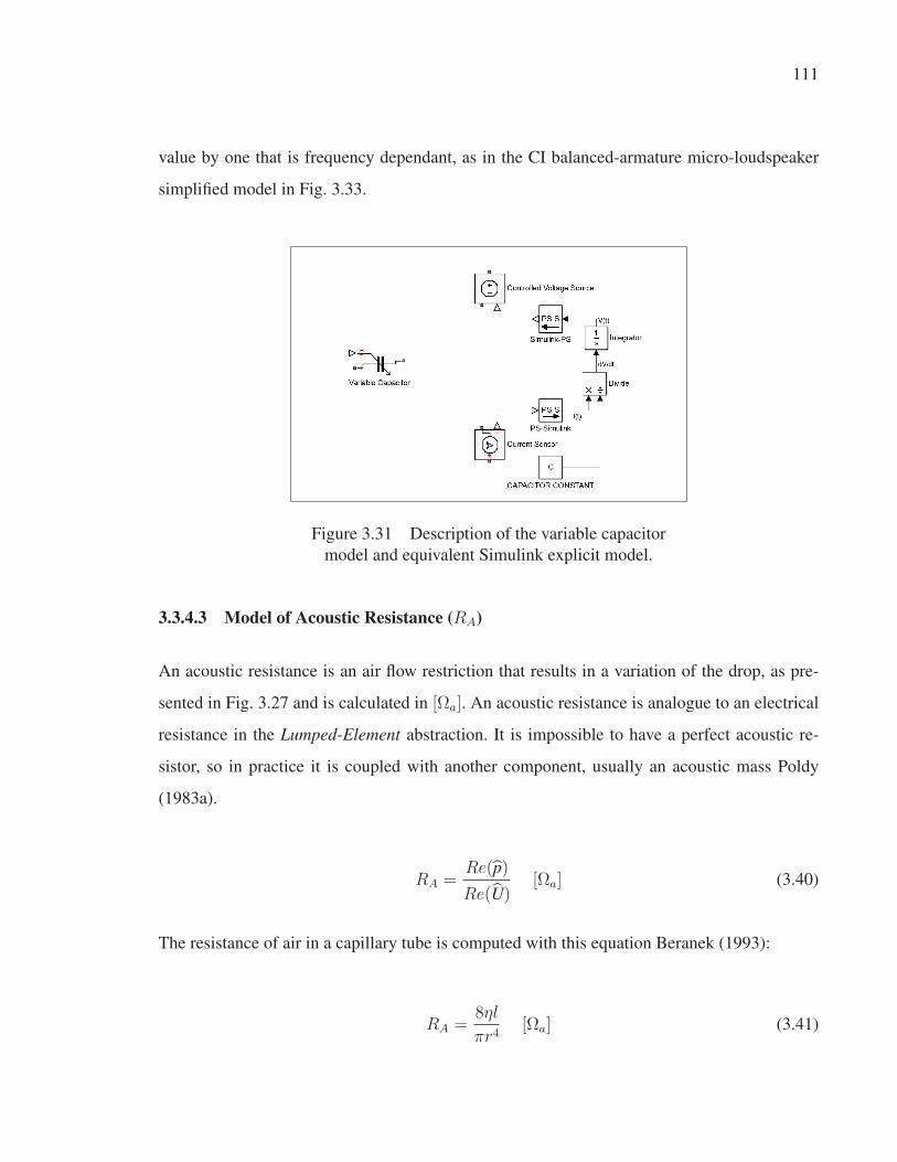
111
value by one that is frequency dependant, as in the CI balanced-armature micro-loudspeaker
simplified model in Fig. 3.33.
Figure 3.31 Description of the variable capacitor
model and equivalent Simulink explicit model.
3.3.4.3 Model of Acoustic Resistance (RA)
An acoustic resistance is an air flow restriction that results in a variation of the drop, as pre-
sented in Fig. 3.27 and is calculated in [Ωa]. An acoustic resistance is analogue to an electrical
resistance in the Lumped-Element abstraction. It is impossible to have a perfect acoustic re-
sistor, so in practice it is coupled with another component, usually an acoustic mass Poldy
(1983a).
RA =Re(p)
Re(U)[Ωa] (3.40)
The resistance of air in a capillary tube is computed with this equation Beranek (1993):
RA =8ηl
πr4[Ωa] (3.41)

112
A different equation is used for the front rectangular tube Rossi (2007):
RA =rpηl
a3b[Ωa] (3.42)
An ideal resistor model is present in Simscape, as shown in Fig. 3.30.
Modelling of micro-loudspeakers response in artificial ears and coupler
This section presents the Lumped-Element and Control System Block diagram models of a
moving-coil micro-loudspeaker and a balanced-armature micro-loudspeaker. It also presents a
Lumped-Element model of an ear simulator.
3.3.4.4 Models of Moving Coil Micro-Loudspeakers
Figure 3.32 Lumped-Element equivalent electrical
impedance circuit of a moving-coil micro-loudspeaker.
A moving coil micro-loudspeaker converts electrical energy into acoustical energy through the
axial movement of a membrane. A comprehensive explanation of how a loudspeaker works is
presented by Borwick Borwick et al. (2001). Two main representations of micro-loudspeakers
are used. The Lumped-Element representation is very popular since the electro-acoustic param-
eters are introduced. They can be inserted into a SPICE network and computed as an electrical
network equivalent Leach Jr. (1991). However, it is necessary to convert electrical components
to acoustical components by using a conversion factor to match the units related to a specific

113
domain. For example, a factor (Bl)2 is necessary to convert the electro-acoustic parameters
into electrical parameters Rossi (2007). The ODEs of the micro-loudspeaker are also presented
in the Control System Block Diagram method. It is possible to integrate it readily into Simulink
as presented in Fig. 3.29 from Strutzer et al. Sturtzer et al. (2012). The model presented by
Sturtzer et al. is thoroughly demonstrated by the author to be a reliable model and will there-
fore not be further explored in this article. However, it will be used in Section 3.3.8 as a hybrid
model combining a Lumped-Element and a Control System Block Diagram to demonstrate the
impact of the solver selection on the time necessary to perform a simulation when a model is
or is not a stiff system. The definition of stiffness is provided in Section 3.3.6.
3.3.4.5 Balanced Armature Micro-Loudspeakers
Figure 3.33 Lumped-element model of the Knowles CI balanced-armature
micro-loudspeaker as reproduced from the documentation provided by Knowles.
Balanced armature micro-loudspeakers are by design nonlinear. Yet, the armature stiffness and
the electromagnetic force acting upon it are proportional and will create a linear behaviour. The
models are generally more complex - nonlinear - than for a moving coil micro-loudspeaker.
Because of this, a modified Lumped-Element model is presented in Fig. 3.33. The CI micro-
speaker model is reproduced from the documentation provided by Knowles®. The ODEs in
Jensen’s work Jensen (2009) are presented in a Control System Block Diagram representation
in Fig.3.34. All the constants and coefficients in the model in Fig.3.34 match Jensen’s work
to facilitate correspondences to its work. The model yields the same results when a Fixed-step
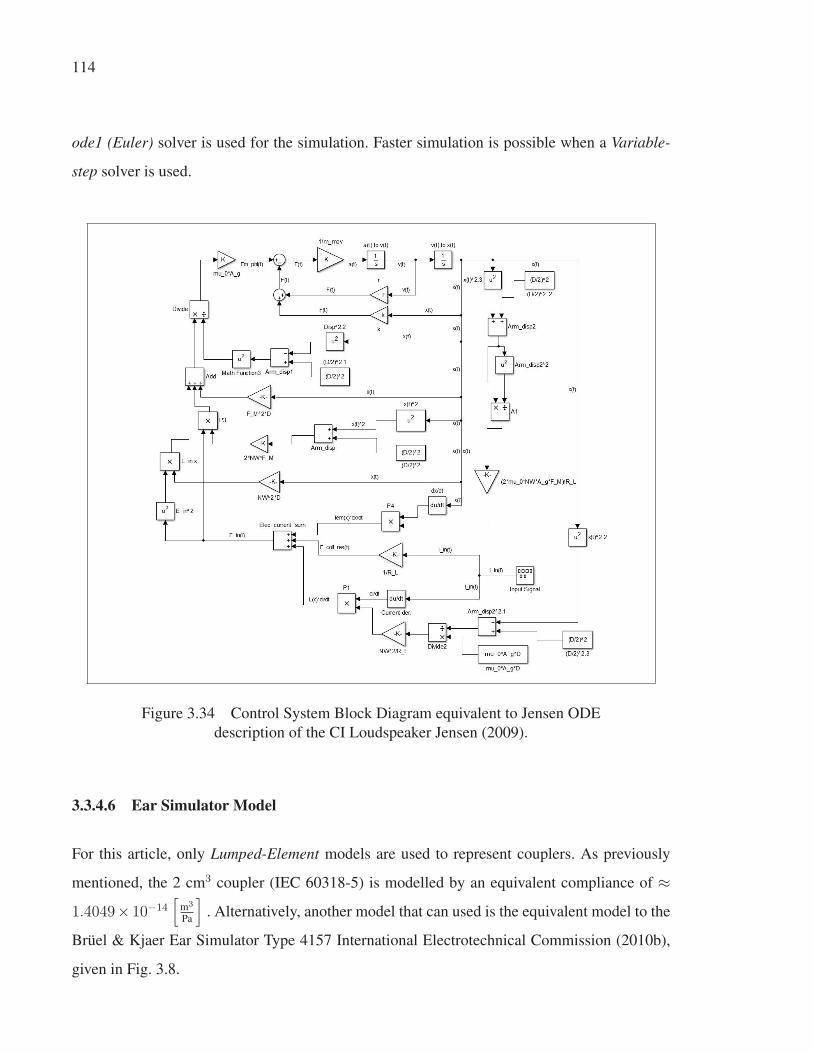
114
ode1 (Euler) solver is used for the simulation. Faster simulation is possible when a Variable-
step solver is used.
Figure 3.34 Control System Block Diagram equivalent to Jensen ODE
description of the CI Loudspeaker Jensen (2009).
3.3.4.6 Ear Simulator Model
For this article, only Lumped-Element models are used to represent couplers. As previously
mentioned, the 2 cm3 coupler (IEC 60318-5) is modelled by an equivalent compliance of ≈1.4049× 10⁻¹⁴
[m3
Pa
]. Alternatively, another model that can used is the equivalent model to the
Brüel & Kjaer Ear Simulator Type 4157 International Electrotechnical Commission (2010b),
given in Fig. 3.8.
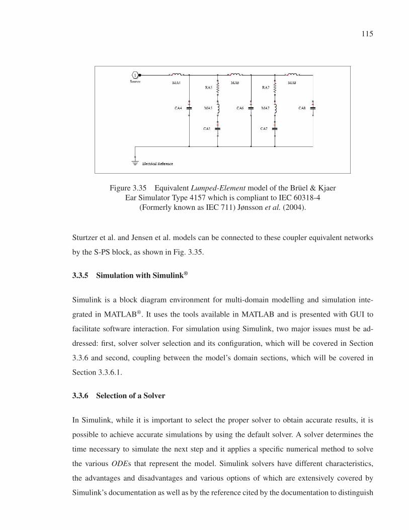
115
Figure 3.35 Equivalent Lumped-Element model of the Brüel & Kjaer
Ear Simulator Type 4157 which is compliant to IEC 60318-4
(Formerly known as IEC 711) Jønsson et al. (2004).
Sturtzer et al. and Jensen et al. models can be connected to these coupler equivalent networks
by the S-PS block, as shown in Fig. 3.35.
3.3.5 Simulation with Simulink®
Simulink is a block diagram environment for multi-domain modelling and simulation inte-
grated in MATLAB®. It uses the tools available in MATLAB and is presented with GUI to
facilitate software interaction. For simulation using Simulink, two major issues must be ad-
dressed: first, solver solver selection and its configuration, which will be covered in Section
3.3.6 and second, coupling between the model’s domain sections, which will be covered in
Section 3.3.6.1.
3.3.6 Selection of a Solver
In Simulink, while it is important to select the proper solver to obtain accurate results, it is
possible to achieve accurate simulations by using the default solver. A solver determines the
time necessary to simulate the next step and it applies a specific numerical method to solve
the various ODEs that represent the model. Simulink solvers have different characteristics,
the advantages and disadvantages and various options of which are extensively covered by
Simulink’s documentation as well as by the reference cited by the documentation to distinguish

116
Fixed-Step from Variable-Step and Explicit from Implicit. Many conditions are involved when
selecting a solver. For instance, fixed-step solvers cannot solve for discrete states and usually
a stiff system, as defined by equation 3.43, is better solved by an Implicit solver. Most of the
block diagrams built in a Control System Block Diagram can be accurately solved by using
the default settings of the software (ode45) which is a variation of the Runge-Kutta method
Kreyszig (2010).
Table 3.7 Definition of terms used to describe various solvers in Simulink
Property DefinitionFixed-Step vs. Variable-Step Fixed-step solvers compute every step of a simulation ac-
cording to the specified timestep while Variable-Step dy-
namically adapts the step size based on the local error
Explicit vs. Implicit An explicit method uses the previous state results to com-
pute the current state while the implicit method must com-
pute the current state as well as the subsequent state to
achieve accuracy.
Continuous vs. Discrete A continuous solver computes the solution for a continuous
integrator while the discrete solver computes the solution
for a system in which the integrator has been replaced by a
discrete equivalent.Note: See Simulink documentation for specificity of each solvers available in the software
When the model includes high stiffness components, the system must be studied more atten-
tively since not all solvers will perform an accurate simulation. By definition, "the stiffness [of
a system] arises from the fact that the system has some eigenvalues [λ] with large magnitude
negative real parts, corresponding to the fast mode, and other eigenvalues with small magni-
tude negative real parts, the slow mode." Hartley et al. (1994). Determination of the eigenvalues
can be done within MATLAB or by several other methods Kreyszig (2010). Once known, the
eigenvalues can be used to compute the stiffness ratio of a system.
Stiffness ratio =max|Re(λ)|min|Re(λ)| � 1 (3.43)

117
"A system is stiff if the timestep [increment of time at which a simulation computation occurs]
required to produce a stable simulation of the system is significantly smaller than the timestep
required to produce an accurate simulation of the system assuming that stability is not an issue."
Hartley et al. (1994). A system is considered slightly stiff when the ratio is greater than 103
and highly stiff when the ratio is greater than 106. Usually, a system corresponding to the high
stiffness criterion, such as certain acoustic models, will be solved by an implicit, variable-step
solver.
3.3.6.1 Coupling Between Domain Sections of the Model
Another aspect of simulating using Simulink is the connection between domains. By default,
Simulink is dimensionless and by using integration or derivation methods, it is possible to ex-
tract a specific state of a vector’s physical quantity such as position, speed and acceleration.
When changing from one physical domain to another, e.g. electrical to mechanical, it is im-
portant to keep track of the transformation between blocks since it might yield unexpected
behaviour from the models because Simulink authorizes most of the connections. This is most
relevant when impedance matching is considered for acoustical, electrical and mechanical sys-
tems. For example, cetain Lumped-Element diagrams use the CGS units reference while others
use the MKS units reference, which can lead to an important mismatch since the ratio of magni-
tude MKSCGS
is 105 for CA and MA. Another important coupling is between Control System Block
Diagram and Lumped-Element section. Lumped-Element uses by analogy p and U as compo-
nents across and through, but Control System Block Diagrams have vector physical quantities
for output. Therefore, transformation of the vector physical quantities - e.g. position, speed
or acceleration - into the across (or through) quantities is necessary; To transform position
| x | ejωt into pressure p, a gain of the air impedance is necessary.
3.3.6.2 Simulating Frequency Response Function and Plotting Poles and Zeros
Electro-acoustic engineers rely heavily on the frequency response function and the phase plot,
commonly known as Bode plot, and the Pole-Zero Plot as design tools. Simulink provides
these plot tools as built-in blocks (see Fig. 3.36). When simulating Lumped-Elements using

118
Figure 3.36 Image of the Bode plot analysis tool
in Simulink.
Simulink, the resulting frequency response curve is usually around -120 dB on the y-axis,
which is about 94 dB less than what would be measured with a physical set-up. The reason for
this is that the ratio of the input over the output is not converted by the Bode plot to Sound
Pressure Level (SPL). Since an input of 1 V is used in the simulation, the ratio to the reference
(Pref = 20×10−6[Pa]) is not taken into account because the ratio 94 dB = 20·log10( 120×10−6 ) is
not by default in the simulation. This particularity has also been noted for the SPICE simulation
Kahrs (2009).
Figure 3.37 A) Section view of a moving-coil
micro-loudspeaker in the enclosure with the B)
Lumped-Element model Rossi (2007).
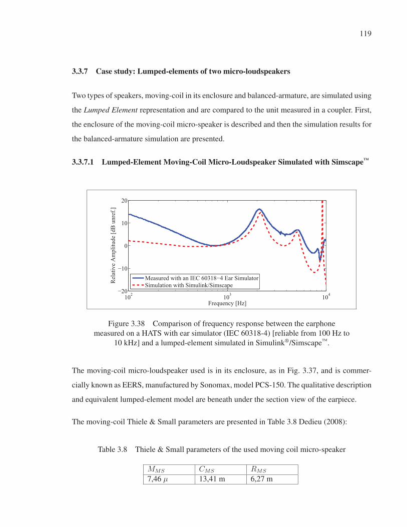
119
3.3.7 Case study: Lumped-elements of two micro-loudspeakers
Two types of speakers, moving-coil in its enclosure and balanced-armature, are simulated using
the Lumped Element representation and are compared to the unit measured in a coupler. First,
the enclosure of the moving-coil micro-speaker is described and then the simulation results for
the balanced-armature simulation are presented.
3.3.7.1 Lumped-Element Moving-Coil Micro-Loudspeaker Simulated with Simscape™
102 103 104−20
−10
0
10
20
Frequency [Hz]
Rel
ativ
e A
mpl
itude
[dB
unr
ef.]
Measured with an IEC 60318−4 Ear SimulatorSimulation with Simulink/Simscape
Figure 3.38 Comparison of frequency response between the earphone
measured on a HATS with ear simulator (IEC 60318-4) [reliable from 100 Hz to
10 kHz] and a lumped-element simulated in Simulink®/Simscape™.
The moving-coil micro-loudspeaker used is in its enclosure, as in Fig. 3.37, and is commer-
cially known as EERS, manufactured by Sonomax, model PCS-150. The qualitative description
and equivalent lumped-element model are beneath under the section view of the earpiece.
The moving-coil Thiele & Small parameters are presented in Table 3.8 Dedieu (2008):
Table 3.8 Thiele & Small parameters of the used moving coil micro-speaker
MMS CMS RMS
7,46 μ 13,41 m 6,27 m
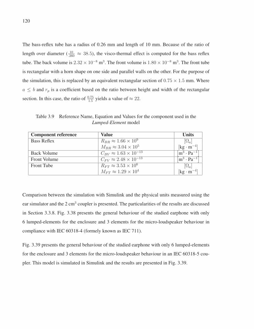
120
The bass-reflex tube has a radius of 0.26 mm and length of 10 mm. Because of the ratio of
length over diameter ( 10.260
≈ 38.5), the visco-thermal effect is computed for the bass reflex
tube. The back volume is 2.32× 10⁻⁸ m3. The front volume is 1.80× 10⁻⁸ m3. The front tube
is rectangular with a horn shape on one side and parallel walls on the other. For the purpose of
the simulation, this is replaced by an equivalent rectangular section of 0.75 × 1.5 mm. Where
a ≤ b and rp is a coefficient based on the ratio between height and width of the rectangular
section. In this case, the ratio of 0.751.5
yields a value of ≈ 22.
Table 3.9 Reference Name, Equation and Values for the component used in the
Lumped-Element model
Component reference Value UnitsBass Reflex RBR ≈ 1.66× 10⁹ [Ωa]
MBR ≈ 3.04× 10⁵ [kg · m−4]Back Volume CBV ≈ 1.63× 10⁻¹³
[m3 · Pa−1
]Front Volume CFV ≈ 2.48× 10⁻¹³
[m3 · Pa−1
]Front Tube RFT ≈ 3.53× 10⁶ [Ωa]
MFT ≈ 1.29× 10⁴ [kg · m−4]
Comparison between the simulation with Simulink and the physical units measured using the
ear simulator and the 2 cm3 coupler is presented. The particularities of the results are discussed
in Section 3.3.8. Fig. 3.38 presents the general behaviour of the studied earphone with only
6 lumped-elements for the enclosure and 3 elements for the micro-loudspeaker behaviour in
compliance with IEC 60318-4 (formely known as IEC 711).
Fig. 3.39 presents the general behaviour of the studied earphone with only 6 lumped-elements
for the enclosure and 3 elements for the micro-loudspeaker behaviour in an IEC 60318-5 cou-
pler. This model is simulated in Simulink and the results are presented in Fig. 3.39.
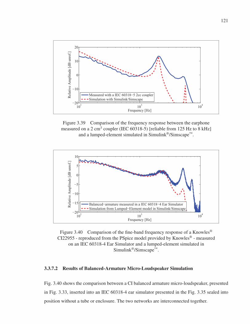
121
102 103 104−20
−10
0
10
20
Frequency [Hz]
Rel
ativ
e A
mpl
itude
[dB
unr
ef.]
Measured with a IEC 60318−5 2cc couplerSimulation with Simulink/Simscape
Figure 3.39 Comparison of the frequency response between the earphone
measured on a 2 cm3 coupler (IEC 60318-5) [reliable from 125 Hz to 8 kHz]
and a lumped-element simulated in Simulink®/Simscape™.
102 103 104−20
−15
−10
−5
0
5
10
Frequency [Hz]
Rel
ativ
e A
mpl
itude
[dB
unr
ef.]
Balanced−armature measured in a IEC 60318−4 Ear SimulatorSimulation from Lumped−Element model in Simulink/Simscape
Figure 3.40 Comparison of the fine-band frequency response of a Knowles®
CI22955 - reproduced from the PSpice model provided by Knowles® - measured
on an IEC 60318-4 Ear Simulator and a lumped-element simulated in
Simulink®/Simscape™.
3.3.7.2 Results of Balanced-Armature Micro-Loudspeaker Simulation
Fig. 3.40 shows the comparison between a CI balanced armature micro-loudspeaker, presented
in Fig. 3.33, inserted into an IEC 60318-4 ear simulator presented in the Fig. 3.35 sealed into
position without a tube or enclosure. The two networks are interconnected together.

122
3.3.8 Discussion on simulating earphones with Simulink®
The modelling method used in this article is a small signal simplification of a complex system:
a micro-loudspeaker in its enclosure. The moving-coil is approximated by a second order elec-
trical network equivalent and while the balanced-armatures have a higher order behaviour, but
they are also simplified. Since the driving pole-zero couple is a second order system, the roll-off
is 40 dB/dec., for frequencies above the resonance. Higher order systems have a steeper roll-
off. To achieve a more accurate simulation, the models can be substituted by a block diagram
model that takes into account nonlinearities and other behaviour inherent to the component as
demonstrated by Sturtzer et al. and Jensen et al., and that were not explored in depth in this
article. A coupling between the models is possible using tools included in the software and are
intended to convert Simulink signals into physical signals. Furthermore, Simscape allows for
the creation of new blocks to include more complex equations that would take into account
visco-thermal effects within the component. However, even a very simple model, that could
be built within an hour provides valuable design information. Resonances, created by faster
pole-zero couples, provide an estimate of the general behaviour of the earphones and if further
development is of interest. The building methods shown in this article are in no way intended
to provide an accurate reproduction on the entire hearing frequency spectrum, which would be
of interest for a designer, but rather to provide a tool to assess whether a design would be worth
further development, or not. If further development is necessary more complex and, but more
accurate methods, such as the four-port network, not covered in this article can be used. As for
other simulation methods, the type of model used, its implementation and solver set-up are the
main variables to a successful simulation.
Two systems are studied with the pole-zero plot. Fig. 3.41 shows the poles and zeros for a
mix elements model and Fig. 3.42 shows the poles and zeros for the simulation of a Lumped-
Element only model. The plots shows what the pole-zero plot provides when a pole is selected.
For the hybrid system, the ratio is:
StiffnessHybrid =10324
69≈ 189 (3.44)
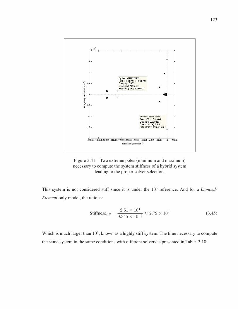
123
Figure 3.41 Two extreme poles (minimum and maximum)
necessary to compute the system stiffness of a hybrid system
leading to the proper solver selection.
This system is not considered stiff since it is under the 103 reference. And for a Lumped-
Element only model, the ratio is:
StiffnessLE =2.61× 10⁴
9.345× 10⁻⁶≈ 2.79× 10⁹ (3.45)
Which is much larger than 106, known as a highly stiff system. The time necessary to compute
the same system in the same conditions with different solvers is presented in Table. 3.10:

124
Figure 3.42 Two extreme poles (minimum and maximum)
necessary to compute the system stiffness of a hybrid system
leading to the proper solver selection.
Table 3.10 Time to compute 1 s of simulation of a hybrid model of Control SystemBlock Diagram connected to Lumped-Element model and only Lumped-Elements model
for different solvers with default setting
Solver Time [s] to complete the hybridsimulation
Time [s] to complete a LumpedElement only simulation
ode45 56.9 ≈ 104
ode23 44.5 ≈ 105
ode113 94 > 105
ode15s* 139.8 0.59
ode23s* 84.3 0.74
ode23t* 50.2 0.48
ode23tb* 47.2 0.47*Implicit solver (suggested for stiff problems)
125
3.3.9 Conclusions
This article is intended as an introduction to Simulink/Simscape as an electro-acoustic design
tool to complete the generic tutorial provided by MathWorks on how to use the tools by ad-
dressing the fundamentals of earphone design with this software. Open-source options, like
Scilab/Xcos, could also be explored to perform simulations. As stated above, Simulink has all
the necessary features to implement models into a Control System Block Diagram as well as
Lumped-Element model and blocks to acquire the frequency response function, pole-zero plot,
etc. These features are very useful to design earphones and are built in the software. Simulink
has potential because it is not limited to a single physical dimension. The accuracy in the time
domain is not explored in depth and solver selection and settings is outside the scope of the
present article, but the intent was to raise awareness so as to keep in mind as a tool for the
simulation of models, even if only to save time. A definition of stiffness and the demonstration
of its impact on the simulation time were made. The topic psycho-acoustic filters that could be
coupled to the model to evaluate the perceived quality of an earphone has not been discussed
but could be a features that could be added to the block library. This article has opened the topic
of using Simulink and Simscape as an acoustical modelling and simulation tool. The authors
feel there is still much to be explored on the topic.
3.3.10 Acknowledgement
This research was conducted at the Sonomax-ÉTS Industrial Research Chair in In-Ear Tech-
nologies (CRITIAS), and was funded by National Science and Engineering Research Council
of Canada and the Fonds Québécois de la recherche sur la nature et les technologies (FQRNT).
The authors would like to thank Tom Hazlett and Janice LoPresti from Knowles Electronics
(Itasca, Il) for their support.
126
3.4 Conclusions on earphone modelling and simulation
This chapter presented the modelling and simulation of earphone for three modelling methods:
the lumped-elements, two-ports and control system block diagram methods. It demonstrated
that it is possible to model adequately earphones with one or several of these methods for the
frequency range in which it can be measured by an ear simulator. The accuracy of the model
and simulation depends largely on the selected modelling method which will have accuracy in
relation to the size of the components intended to be modelled. In complement, an extensive
library of models necessary to model earphones is listed for each modelling method.
This chapter also identified powerful simulation tools which provide the flexibility and the
capability to implement the various modelling methods into a single interface. This chapter
focused on the use of Simulink because its important presence in the engineering world and
its capability to be use in synergy with other tools such as finite elements softwares. It demon-
strated that Simulink is a tool with all the features necessary to adequately simulate design of
earphone.

Chapter 4
FUTURE WORKS
This chapter identifies two areas in need of research in order to offer to earphone designers
the tool they need to control the development of their earpieces. The first work identified is
the improvement of the measurement apparatuses, which are limited in the frequency band it
is reliable when compared the entire human hearing spectrum. The second work is a proper
assessment of the psycho-acoustic impact of the coupling between the earphone and the ear.
Previous studies identified a large variability related to this topic. However, the impact of this
variability on the perceived quality is not yet defined in the literature.
Another topic discussed in this chapter is a proposed approach to address the issue of the vari-
ability of the coupling between the earphone and the user’s ear. It is suggested that leaving to
the user the control of the perception description and embedding the frequency response cor-
rection in a background run application would be the best way to address the issue of coupling.
Furthermore, it is suggested that a cross-device compatibility is a key component of the success
of this approach.
4.1 Improvement of the measurement apparatuses
As presented in Chapter 2, the normalized measurement tools available at the time of the writ-
ing of this thesis provides reliable measurement in a range of 100 Hz to 10 kHz. Human hearing
range is accepted to be from 20 Hz to about 20 kHz. In this regard, the limited ability of the ear
simulator, which measure about 70% of the frequency range typically heard by a human, limits
the ability to evaluate a proper design. The earphone designer rely heavily on his experience as
well as a very quiet surrounding for compensation.
Another limitation of the actual measurement tools is that they replicate the response of an
average ear, while the variability of the human ear frequency response is important, as it is
explained in the next section.

128
It is suggested that a new type of manikin with an ear simulator that would also simulate the
variability of the ear canal as well as being able to measure an extended frequency response
would be a great improvement for designers.
4.2 Assessment of the psycho-acoustic impact of the coupling between the earphone and
the ear
Many studies measured the variability of individuals in-ear response, for example Hammershøi
and Møller (1996), as well as the coupling between the ear and the earphone (Møller et al.
(1992) and Ciric and Hammershøi (2006)). From an amplitude point of view, as explained in
Chapter 1, this variability is significant. It ranges from several dB around 2 kHz up to 30 or
40 dB above 8 kHz. It is also known that the Just Noticeable Sound Change (JNSC) is small
compared to the variability, in the order of magnitude of 1 to 5 dB. The objective and subjective
research suggest that the coupling of the ear with the earphone will have a significant impact
on the perceived quality of an earphone, when it is evaluated by a large panel of subject.
The same observation can be made for the variability in the position of the ear canal resonant
frequency. Positioned on average around 2.7 kHz, it can range from 2 kHz up to 3.5 kHz.
Such difference between the natural resonance of the ear canal and an earphone designed to
replicate the average seems to be of a noticeable nature by an individual lying in the extreme
of the measured population.
However, is this variability an issue or not? Most of the study as of now aim at identifying an
average frequency response that would be the starting point for the development of the next
generation of earphone. They do not evaluate if this average will be suitable for a large group.
For example, a well known contributing factor to the perceived quality of sound is sealing the
ear with the earphone, which have a known impact of a perceived fullness of sound. The lack of
bass is a well known critic of many earphones. The source of these critics is already addressed
by several approach available on the market which ensure that the ear canal is sealed by the
earphone.
129
Since the variability of the human ear is known, it is suggested to take advantage of this knowl-
edge to offer a customization process to the user, discussed in the next section.
4.3 Enhancing user experience through customization
One common observation is that all the earphones on the market up to now are push demand
products, based on strong marketing and off the shelf design. Olive’s experiments have re-
peatedly demonstrated that people, even groups of people who sometimes use lower quality
sources, prefer good sound reproduction. This trend is unlikely to change and would comply
with a study by Pralong and Carlile (1996) stating that a personalized equalization is better
than a generic equalization for headphones, distortion wise. Customers will not change their
buying habits except if a new way of buying earphones is presented to them, basically because
they are accustomed to the actual offering. However, if a new set of performance metrics is
presented, like the possibility of defining a sound signature that would be specific to the user,
the improvement in quality would be appreciated by the users, as noted by Keiper (1997):
In today’s highly competitive markets, manufacturers all over the world might
actually use the same machinery and the same raw materials to make their product.
It is the product engineering and design where the differentials between similar
products come in. Since everybody can hear and perceive acoustic quality (and
claim to be an expert), good acoustic engineering and design are needed and rep-
resent an excellent chance of market success.
This quote is about any consumer’s product, from hair dryers to washing machines, but cannot
be more true for earphones and consumer electronics as a whole. Users expect improvement in
the product they buy. They expect that every iteration will be more satisfying than the previous
version. It is highly unlikely that earphone offering will differ from other consumer products
where mass-customization - or personalization - will occur when the product offering shifts
from goods to experience products, as noted by Davis (1997) because consumers will look
for the product that would do the best job for them, not a one size fits all. A legitimate ques-
tion arises from these observations: Toward which personalization should earphones designers
130
orient their efforts? Based on previous sound quality research, it is likely that, at some point,
customers will expect a sound that would really reflect their preference, and not an ideal defined
in a remote lab.
On this, the author suggests that consumers would rather choose the sound signature they prefer
for their earphones by presetting the relative loudness of bass, mid and treble. Their person-
alized sound signature would be reproduced on any compatible device at any moment based
on their preferences. Customization of the frequency response is expected to be performed not
the modification of the earphone itself but by the programming of the playback device. The
device would recognize the earphone by an identification chip embedded in the earphone on
which the description of the earpiece is stocked and then returned on the different smart de-
vices to recall the user’s preferences. It would produce a high-end product with features that
would empower the end-user by addressing the issue of intra/inter-subject variability. The by
default sound signature could be one such as proposed by Olive et al. (2013) so the average
person would already have a preset quality sound. For those who deviate from the average, this
compensation option would allow them to use the earphone to its fullest capacity.
4.3.1 Post-setting the relative loudness of earphones
As suggested previously, it is unlikely that a universal frequency response function satisfies
every consumer. It is necessary to give to the consumer the opportunity to adjust the frequency
response function by an easy and interactive tool. This tool would articulate around anchors
defined in amplitude as well as center frequency that would be modified based onto the user’s
preference. These anchors are necessary to match the main ingredient of earphone frequency
response matching, an accurate bass reproduction. The resonance of the ear canal and the ex-
tension in the high frequencies, associated with the brilliance of the sound, as presented in
Figure 1.11. These criteria are chosen for the agreement in the literature of their impact on
sound quality ratings. It is expected that not all users are seasoned in audio, and there is a need
to broaden the typical equalizer to descriptors that would be significant to users using what is
already present for naive psycho-acoustic studies. For example, a user could have the option

131
to describe its earphone sound as too bassy or lacking bass which would be translated in an
increase by the system.
4.3.2 Using the impedance frequency relation for compensation
In Chapter 2, the relationship between the frequency response and the impedance is demon-
strated. There is also a demonstration of the impedance resonance variation when a air load is
applied to the earpiece. Based on this concept, it is possible to assess the coupling between the
ear and the earphone and correct the frequency response accordingly in order to provide the
frequency response expected by the user without the user’s intervention. When used combined
to the user preference, this approach would allow for a better music listening experience.
4.4 Conclusions on future works
The future works identified in this chapter all have a common root, the variability of the cou-
pling between the earphone and the ear of the users, which is known to be large and its impact
not well known. Three approaches to this issue are proposed, which could be implemented in
altogether or singularly. The first one is to study the relation between the coupling of the ear-
phone with the ear and the impact of this coupling from a psycho-acoustic point of view for a
large population and assess if there is a correlation and of what nature it is, if there is one.
The second proposed approaches is to develop measurement apparatuses that would allow
designers to assess how their design perform for a larger population. In this case, the apparatus
would have to replicate the variability of several features of the human ear anatomy in order to
modify the in-ear response to replicate the variability of the population.
The third approach would be to take advantage of the, nowadays, largely available signal pro-
cessing capabilities found in many device music listeners use to listen to their music. By using
the relationship between the measurement of impedance and the frequency response when the
earphone is under the same load, it is possible to adjust the earphone to correct for the preferred
frequency response identified by the user. Therefore avoiding the issue to design multiple phys-
ical earphone to match many user preferences.


CONCLUSION
This thesis aims at identifying the contributing factors to a good sound signature and also
explains the other components contributing to a proper earphone design. In Chapter 1, it is
demonstrated that earphone frequency responses are, nowadays, as different as the exterior de-
sign of the earpiece. This is partially because of design philosophies, but also because there
is no unequivocal agreement on what a proper frequency response for an earphone, or for a
headphone, should be. A tendency for a compensation that would replicate the head related
transfer function in a specific field is prevalent, but the variability of the human anatomy, when
analyzed on a large scale, tends to limit the applicability of any study reporting a specific fre-
quency response based on this premise. Many studies already explored this approach and none
were deemed satisfactory when re-evaluated by other researchers. Furthermore, the consumers’
expectations is high not only toward earphone build quality, but also in sound quality. Several
areas are still in need of research and development in order to achieve a design based on re-
liable data. How to handle the variability of the impedance coupling between the ear and the
earphone still presents the most challenges.
In Chapter 2, the measurement methods for earphones and the tools available have been pre-
sented. It is demonstrated that the measurement apparatuses available at the moment are limited
for earphones development. Commercially available ear simulators would typically provide an
accurate frequency response, when compared to a group of subjects, up to 8 kHz. At the other
end of the frequency spectrum, the correlation of the measurement drops significantly under
100 Hz, leading to unreliable measurement for four octave bands, two at each end of the hearing
spectrum. These octave bands are known to provide the sensation of power and brilliance, two
very important attributes of so-called high-fidelity reproduction when compared to low-fidelity
reproduction. A manikin that would be adaptable so as to reproduce a various array of shapes
of the external ear would greatly improve the assessment of the variability in the frequency
response which would have an impact on sound quality. The development of an extended fre-
quency range measurement apparatus would allow a designer to confirm that his design will
offer a good frequency response for a known percentage of the population.
134
A contrario to the psycho-acoustic models discussed in Chapter 1, the models of acoustic
transducers and passive acoustical components have been studied extensively and their lim-
itations are well recognized, as presented in Chapter 3. In light of this, it is possible for an
earphone designer to match a desired target frequency response with the design tools available.
The complementarity of the levels of abstraction and the software available contribute to this
capacity. Furthermore, the improvement of finite element multi-physics analysis, not covered
in this thesis, allows for accurate determination of how an earphone would respond to a spe-
cific stimulus. While models and modelling methods have greatly improved, the actual tools
for measurements seems inadequate to confirm that a physical model actually behaves as per
design.
Chapter 4 presents two future works to help earphone designers in the design of earpiece that
would provide music reproduction with fidelity. The first one is to study the variability of
the coupling between the ear and the earphone in order to include it into a design plan. The
second is to develop a measurement apparatus that would reliably replicate the variability of
the coupling by reproducing a large array of ear shape. An alternate approach, also presented
in Chapter 4, suggests that the frequency response of an earphone should be modified on an
individual basis since any music player released in the near future will have the necessary signal
processing capabilities to correct for the frequency response desired by a user. Two challenges
exist for this approach. The first challenge lies in the making of a user-friendly interface, easy
to understand for a non-specialist, who might have a great interest in good music reproduction
without necessarily wanting to learn how it is achieved. The second challenge would be to
make this individualized response cross-platform and cross-device so the user is not limited to
a single device, or operating system.
In retrospect, most of the tools necessary for a proper earphone design, as positioned in Fig-
ure 0.1, are already available. Measurement methods and models, either physical or psycho-
acoustical, have extensively been studied. However, several areas are still in need of research
and development in order to achieve a design based on reliable data. This seems to be mostly
because the coupling of the earphone to the ear, which is very variable from one individual to

135
another. It induces a variability in sound quality which is much less prevalent when the music
reproduction is performed with a distant source. When it comes to earphone sound quality and
design, it is no longer a question of how to achieve the two, but rather an understanding of who
are the users and what their expectations are.


APPENDIX I
SMALL-SIGNAL APPROXIMATION OF A MOVING-COILMICRO-LOUDSPEAKER
This section presents the equation of the small-signal approximation of a moving-coil micro-
loudspeaker. This analysis is a complement to the measurement of the speaker impedance curve
presented in section 2.1. From this measurement, it is necessary to identify FS , the resonant fre-
quency of the driver. At that frequency, the impedance value is denoted ZMAX . The parameters
CAS , MAS and RAS are used in section 3.2.3
r0 =Zmax
RE
(A I-1)
|Z| = √r0RE (A I-2)
QMS =FS
√r0
F2S − F1S
(A I-3)
QES =QMS
r0 − 1(A I-4)
The subscript AC stands for Alternative Compliance (AC) as many methods can be used to
modifiy the load on the transducer and therefore shift the peak of the impedance curve.
QMAC =FAC
√r0
F2AC − F1AC
(A I-5)
QEAC =QMAC
r0 − 1(A I-6)

138
QTS =QMSQES
QMS +QES
(A I-7)
VAS = VT
[FACQEAC
FSQES
− 1
](A I-8)
CAS =VAS
1000ρ0c2(A I-9)
MAS =1
4π2F 2SCAS
(A I-10)
MAAC = MASF 2S
F 2AC
(1 +
VAS
VT
)(A I-11)
BL =
√2πFACREMAACS
2D
QEAC
(A I-12)
RAS =BL2QES
QMSRES2D
(A I-13)
η0 =
(4π2
c3
)(F 3SVAS
QES
)(A I-14)
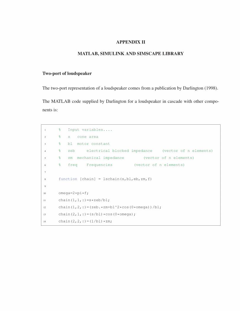
APPENDIX II
MATLAB, SIMULINK AND SIMSCAPE LIBRARY
Two-port of loudspeaker
The two-port representation of a loudspeaker comes from a publication by Darlington (1998).
The MATLAB code supplied by Darlington for a loudspeaker in cascade with other compo-
nents is:
1 % Input variables....
2 % s cone area
3 % bl motor constant
4 % zeb electrical blocked impedance (vector of n elements)
5 % zm mechanical impedance (vector of n elements)
6 % freq Frequencies (vector of n elements)
7
8 function [chain] = lschain(s,bl,eb,zm,f)
9
10 omega=2*pi*f;
11 chain(1,1,:)=s*zeb/bl;
12 chain(1,2,:)=(zeb.*zm+bl^2*cos(0*omega))/bl;
13 chain(2,1,:)=(s/bl)*cos(0*omega);
14 chain(2,2,:)=(1/bl)*zm;

140
Two-port of a tube
A small tube with and without visco-thermal effects is presented by a two-port:
1 function [ output ] = tube( freq, l, r, method )
2
3 omega_i=2*pi*freq;
4
5 if method==1 %Basic
6
7 c_0=353.027;
8 gamma=1i*(omega_i./c_0);
9 output=[cosh(gamma*l) sinh(gamma*l); sinh(gamma*l) cosh(gamma*l)];
10
11 if method==2 %Egolf
12
13 omega(1,1,:)=2.*pi.*freq;
14
15 l_n=l;
16 rho=1.1385; %approximated density of air (37 C)
17 sigma_pr=0.71256; %approximated Prandlt number of air (37 C)
18 mu=1.6696e-5; %absolute viscosity of air (37 C)
19 gamma=1.401; %Heat specific ratio of air (37 C)
20 c=353.027; %speed of sound in air (37 C)
21
22 alpha(1,1,:)=sqrt((-1i.*omega.*rho.*sigma_pr)./mu);
23 beta(1,1,:)=sqrt((-1i.*omega.*rho)./mu);
24
25 Z_n(1,1,:)=((rho.*c)./(pi.*r^2)).*sqrt(1-((2.*besselj(1,beta.*r)./...
26 (beta.*r.*besselj(0,beta.*r)))).*(1+2.*(gamma-1).*...
27 (besselj(1,alpha.*r)./(alpha.*r.*besselj(0,alpha.*r)))));
28
29 Gamma_n(1,1,:)=(1i.*(omega./c)).*sqrt((1+2.*(gamma-1).*...
30 (besselj(1,alpha.*r)./(alpha.*r.*besselj(0,alpha.*r))))./...
31 (1-(2.*besselj(1,beta.*r))./(beta.*r.*besselj(0,alpha.*r))));
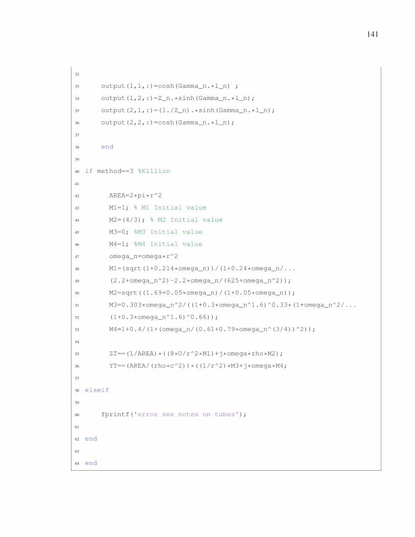
141
32
33 output(1,1,:)=cosh(Gamma_n.*l_n) ;
34 output(1,2,:)=Z_n.*sinh(Gamma_n.*l_n);
35 output(2,1,:)=(1./Z_n).*sinh(Gamma_n.*l_n);
36 output(2,2,:)=cosh(Gamma_n.*l_n);
37
38 end
39
40 if method==3 %Killion
41
42 AREA=2*pi*r^2
43 M1=1; % M1 Initial value
44 M2=(4/3); % M2 Initial value
45 M3=0; %M3 Initial value
46 M4=1; %M4 Initial value
47 omega_n=omega*r^2
48 M1=(sqrt(1+0.214*omega_n))/(1+0.24*omega_n/...
49 (2.2+omega_n^2)-2.2*omega_n/(625+omega_n^2));
50 M2=sqrt((1.69+0.05*omega_n)/(1+0.05*omega_n));
51 M3=0.303*omega_n^2/((1+0.3*omega_n^1.6)^0.33*(1+omega_n^2/...
52 (1+0.3*omega_n^1.6)^0.66));
53 M4=1+0.4/(1+(omega_n/(0.61+0.79*omega_n^(3/4))^2));
54
55 ZT==(1/AREA)*((8*U/r^2*M1)+j*omega*rho*M2);
56 YT==(AREA/(rho*c^2))*((1/r^2)*M3+j*omega*M4;
57
58 elseif
59
60 fprintf('error see notes on tubes');
61
62 end
63
64 end

142
Example of a Simscape program
Simscape components use the branch approach with a variable across and a variable through
defined in chapter 3.
1 component capacitor < foundation.electrical.branch
2 % Capacitor
3 % Models a linear capacitor. The relationship between voltage V and
4 % and current I is $I=C*dV/dt$ where C is the capacitance in farads.
5 %
6 % The Initial voltage parameter sets the initial voltage across the
7 % capacitor. Note that this value is not used if the solver ...
configuration
8 % is set to Start simulation from steady state.
9 %
10 % The Series resistance and Parallel conductance represent small
11 % parasitic effects. The parallel conductance can be used to model
12 % dielectric losses and the series resistance used to represent the
13 % effective series resistance (ESR) of the capacitor. Simulation of
14 % some circuits may require the presence of the small series resistance.
15 % Consult the documentation for further details.
16
17 % Copyright 2005-2008 The MathWorks, Inc.
18
19 $ parameters
20 c = { 1e-6, 'F' }; \% Capacitance
21 v0 = { 0, 'V' }; \% Initial voltage
22 r = { 1e-6, 'Ohm' }; \% Series resistance
23 g = { 0, '1/Ohm' }; \% Parallel conductance
24 end
25
26 variables
27 vc = { 0, 'V' }; \% Internal variable for voltage across ...
capacitor term
28 end

143
29
30 function setup
31 if c ≤ 0
32 pm_error('simscape:GreaterThanZero','Capacitance')
33 end
34 if g < 0
35 pm_error('simscape:GreaterThanOrEqualToZero','Parallel ...
conductance')
36 end
37 if g == {inf, '1/Ohm'}
38 pm_error('simscape:LessThan','Parallel conductance','inf')
39 end
40 if r < 0
41 pm_error('simscape:GreaterThanOrEqualToZero','Series ...
resistance')
42 end
43 if r == {inf, 'Ohm'}
44 pm_error('simscape:LessThan','Series resistance','inf')
45 end
46 vc = v0; \% Assign initial voltage
47 end
48
49 equations
50 v == i*r + vc;
51 i == c*vc.der + g*vc;
52 end$

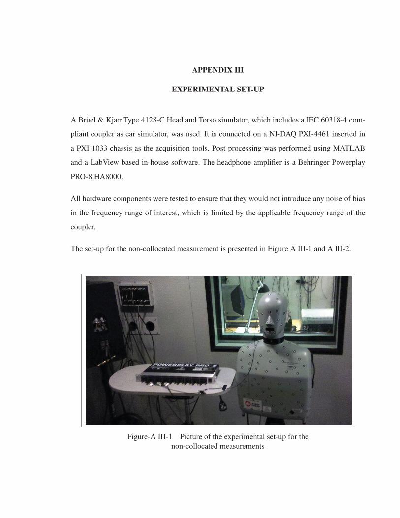
APPENDIX III
EXPERIMENTAL SET-UP
A Brüel & Kjær Type 4128-C Head and Torso simulator, which includes a IEC 60318-4 com-
pliant coupler as ear simulator, was used. It is connected on a NI-DAQ PXI-4461 inserted in
a PXI-1033 chassis as the acquisition tools. Post-processing was performed using MATLAB
and a LabView based in-house software. The headphone amplifier is a Behringer Powerplay
PRO-8 HA8000.
All hardware components were tested to ensure that they would not introduce any noise of bias
in the frequency range of interest, which is limited by the applicable frequency range of the
coupler.
The set-up for the non-collocated measurement is presented in Figure A III-1 and A III-2.
Figure-A III-1 Picture of the experimental set-up for the
non-collocated measurements
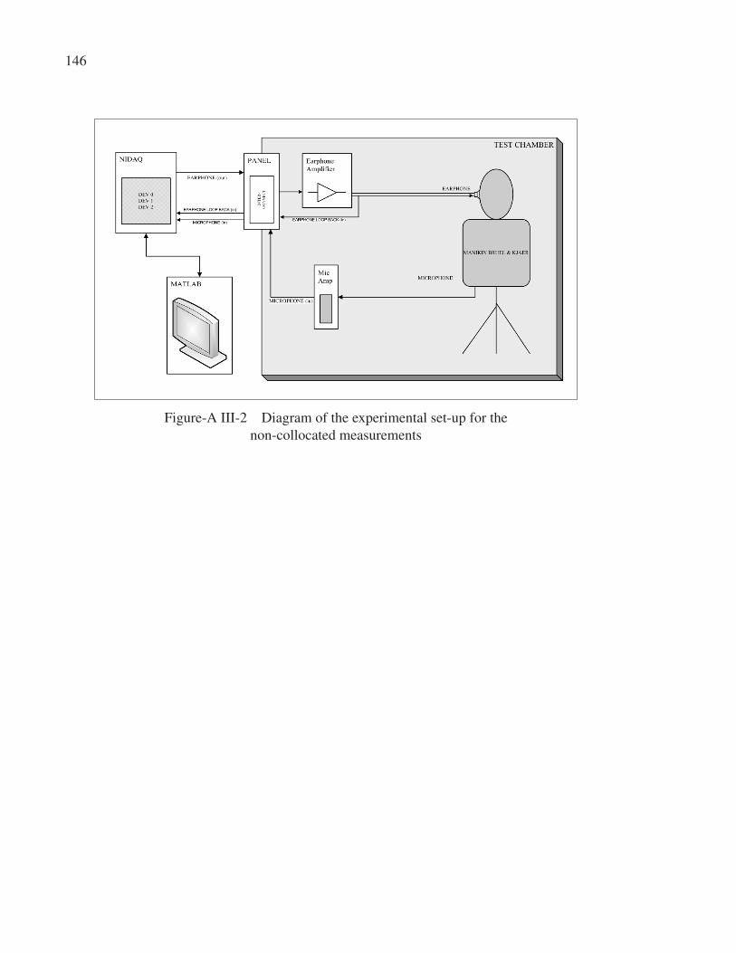
146
Figure-A III-2 Diagram of the experimental set-up for the
non-collocated measurements
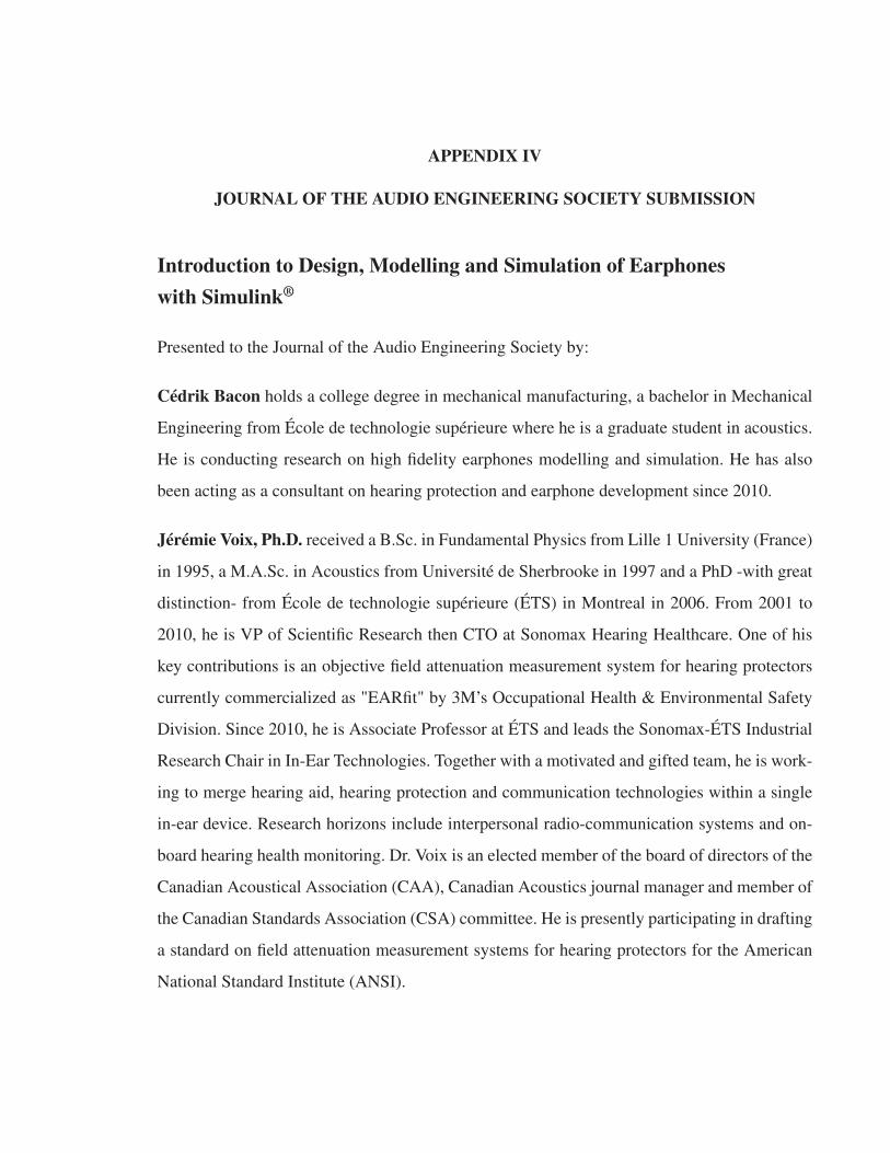
APPENDIX IV
JOURNAL OF THE AUDIO ENGINEERING SOCIETY SUBMISSION
Introduction to Design, Modelling and Simulation of Earphoneswith Simulink®
Presented to the Journal of the Audio Engineering Society by:
Cédrik Bacon holds a college degree in mechanical manufacturing, a bachelor in Mechanical
Engineering from École de technologie supérieure where he is a graduate student in acoustics.
He is conducting research on high fidelity earphones modelling and simulation. He has also
been acting as a consultant on hearing protection and earphone development since 2010.
Jérémie Voix, Ph.D. received a B.Sc. in Fundamental Physics from Lille 1 University (France)
in 1995, a M.A.Sc. in Acoustics from Université de Sherbrooke in 1997 and a PhD -with great
distinction- from École de technologie supérieure (ÉTS) in Montreal in 2006. From 2001 to
2010, he is VP of Scientific Research then CTO at Sonomax Hearing Healthcare. One of his
key contributions is an objective field attenuation measurement system for hearing protectors
currently commercialized as "EARfit" by 3M’s Occupational Health & Environmental Safety
Division. Since 2010, he is Associate Professor at ÉTS and leads the Sonomax-ÉTS Industrial
Research Chair in In-Ear Technologies. Together with a motivated and gifted team, he is work-
ing to merge hearing aid, hearing protection and communication technologies within a single
in-ear device. Research horizons include interpersonal radio-communication systems and on-
board hearing health monitoring. Dr. Voix is an elected member of the board of directors of the
Canadian Acoustical Association (CAA), Canadian Acoustics journal manager and member of
the Canadian Standards Association (CSA) committee. He is presently participating in drafting
a standard on field attenuation measurement systems for hearing protectors for the American
National Standard Institute (ANSI).

������
����������� �� �� �� ������� ��� ��������
�� ��������� ��� ������ �� �
������� ��� ��� ������ ��� ��������� ���� ����� ����������� ������������� ������������� ���������
������ �� ��������� ����������� ��������� �����
�������������� �� ����� �� ���� ��� � �������� ������� ������ �� ������ �� ���
�������� �������� ���������� ������� �� ������� ����� �� ��� ����� ������� ��
�������� �� �������� ��� ���������� �� ����� ��� ������������ �� �� �������� ����
������ �������� �� ���� ��� ����� ���� ������� ��� ��� ������ �� �� ����� ��
���������� ������ ���� ����!�� ���!� ��� ������������ ����� !��� �� ������ !����
������ �� ��� �������� �� "�#���� � ��� �������� ������ �� �������������� �� �������
�������� ���� �� ������ �������� ��� � ��������������� ����� � !��� � �� �������
��� � ����� ������� �� ����� �� ����� �� �������$ ������ ������������� � !���
� ������� ���!��� �� ��� �������� ��� ��� �� ����� �� ��� �������� �� ������ ��
�������� !��� ������ �� ������� �� ��������� �� �� ������� � ��� ��������
� ������������
���� ����� ����� ��� ��� �� �� ������� �� �� ��
�������������� �� �������� �� ��� �������
��� �� ������ ������������� �� � ���� �������
������ ���� �� �������� �� �� �������� ���� �� ����
����� ��� ��� �� �� ����� ���� �� �� ��������
���� ������� �������� ��� � �� �� ������ �����
�������� ������� ��� �������� ���� � !" ��� ������
��� �� �� ����� �� � ���������� �������������
���� ���� #�� ���� ���� �� � ����� �� �����
���� � $"� �%&'( �� ��� ������ � �� � ���� �����
�� ������� )�������� ������� ����� ���� ���������� ��
������ ����� ����� ���������� �� *� �+�� ,�
����� -����� ����� ����� �� �� ������ � �� �����
���� ./0&1 ���� ���� � �� ��� �� ��� ����� ����
������ �� ���� ���� ������� ������ �� ����� � ��
���� � �� ���� ���� 2����� �������� ��� �� �
������ �� ��������� �� ���������
� ����� ����� �
�� ��������� ��� �� ��� �� ��������� ������� ����
��� ���� ���� ��������� ��� ������� �� �� ����
���������� ���� ����� ����� ��� �� ��� ���� ��
������������� �� ������ �� ��� ���� !������ ��
������ � &� ������ ��� �� �� ���� ��������� ������
���� �� �� ������������� ����������� �� ������ $ ��
��� �� ���� �� �� )������ �� ��� �� ���� �
�� �������� .&(' 345 6�!1 �� � $ ��� ����� .&('
�%������������� ����� �� �������� �� &�� ' (��(� �� )��# ���*
+,�-,.�/01�2./3$ �� ��* 4��� ������#5��� ����
345 6�71 ������ �������� &� ��� ������ ��� ���� ��
�������� ������� ���������� �� ����� ���������
�� ���� ��������� �� �� ������������� �� ������
�� ��� ���� !������ �� ��� ���� � �� ������ 5� &�
������ !� ������������� �� �� ��������� �� ����� �
������ �� �� � ����� �� �� ����� �� ������
�� �� �������� �� ������� ����� �� �� �� ������
7�
� �� �������� �! "���##��$ "��%��
�� �� � �� ������� �������� ����� �� ����
���� ����������� �� ��� ����� �� � ������� ���8
!�����������"���#���� �$����� �� �� ��� ����������
����������� ��� �������������� �� ������ �� ���
���� !������ �� ������ ����������� ���� � ����
�� �� ������� � 9"� �$"� � 7"� '�������� �� �� ��� ���
���������� ���� ������ ����������� ��� � � ����� 0��
��� ������� ���� ��� �� �� � �� ��� �� ����� ��
�� ������� ������ ������� �� ������ �� � ���
�� ���������� �� ����� ����� �� ����� ���� ������ �����
��� ���� �� �� ������������ �� ��� �� ������
��� �� ��������
��� ������& ��''����(�) �*+(��� ����''����(�) �),�-�� �*+(���
������ �� �������� )������� ���� �� ���:�� �� ��
������ ����������� �� �� !���������� "���#���� �$���
��� .!"��1� - !"� ������� ������� ����������� ��
�� �� &� ;�4 !"� �� %������ !���������� �$�����
�� ��� �� � ����� ���� �� ��� �� ���� ��� �
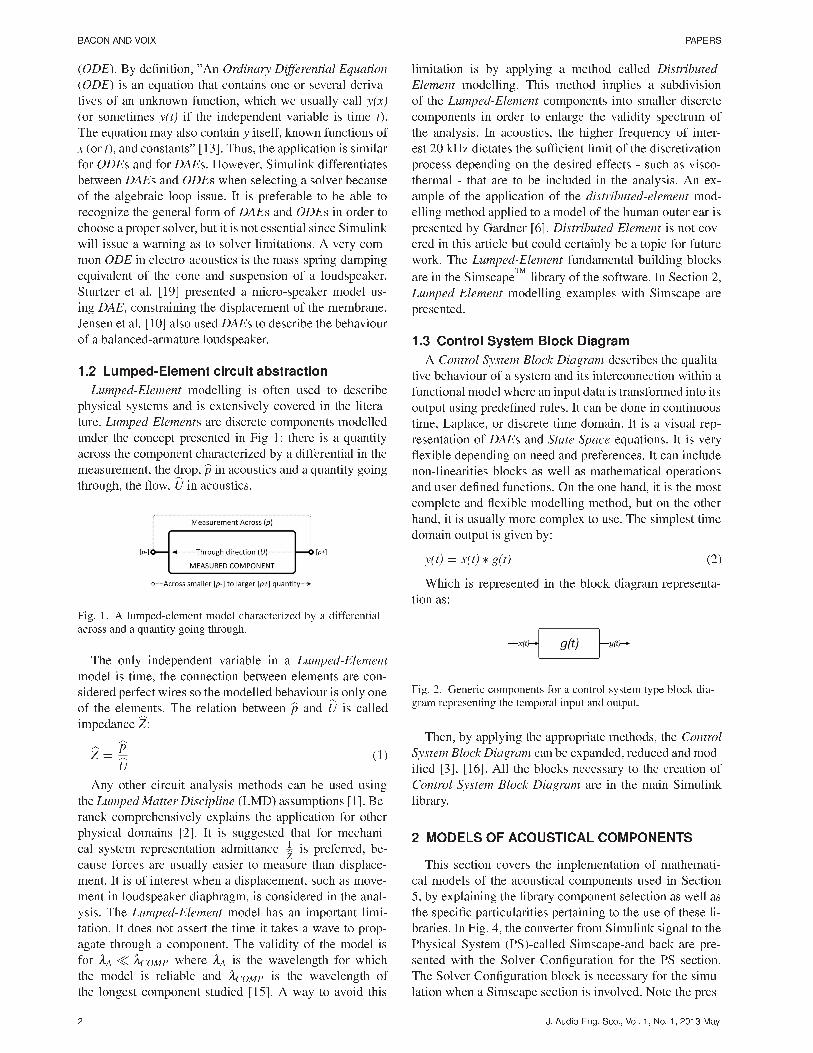
����� ��� ��� ���
������ �� ����� �� ������� ��������� ��������
����� � � ������ ���� ����� �� �� ������� ������
���� �� � ���� ����� ���� �� ������� ���� ���
��� �������� ��� � ��� ������� ������� � ��� ���
�� ������ ��� ���� ���� ����� ��� ������ ��
� ��� �� �� �������� !"#$� ��� ��� �������� � �����
��� ���� �� ��� ����� %������ &���� �����������
������ ���� �� ���� ��� ������' � ������ �������
�� ��� ��'����� ���� ����� (� � ���������� �� �� ���� ��
����')� ��� '����� ���� �� ���� �� ���� ����� ��
������ � ������ ������ ��� � � �� ������� ��� &����
��� ���� � ���' �� �� ������ �������� � ���� ����
�� ��� ���������������� � ��� ��������'�����'
�������� �� ��� ��� �� ������� �� � ������������
&����)�� �� ��� !"*$ �������� � ������������ ����� ���
' ��� ������' ��� ���������� �� ��� ��������
+��� �� ��� !",$ ���� ���� ���� �� ������� ��� ��������
�� � ���������������� ������������
��� ���������� � ������� ����������
�������� ����� ������' � ���� ���� �� �������
������� ������� �� � �-������� ������� ��� ������
����� �������� ������ ��� ������� �������� ��������
���� ��� ������ �������� .' "/ ����� � � ������
������ ��� ������� ���������)�� �� � ��������� ���
���������� ��� ���� �� �������� �� � ������ '�'
�����'� ��� 0�� �� ���������
���� �� � ���� ������ ���� ������������� �� � ������������
������ ��� � �������� ����� ��������
�� ��� ������� ������� � �������� �����
����� � ��� ��� ������ ������ ������� ��� ���
������ ������� ���� �� ��� �������� �������� � ��� ��
�� ��� �������� �� ������ ������ �� �� �� � ������
������� ��1
�� ���
���"�
�� ����� ����� ������ ������� �� �� ���� ��'
��� ������ ������ ������ ��� �234� ��������� !"$� ���
���� ������������� �-���� ��� �������� ��� �����
������� ����� !5$� (� � ��''����� ���� ��� ������
��� ������ ����������� �������� �
��� ��������� ���
����� ������ ��� ������� ����� �� ������� ��� ��������
���� (� � �� ������ ��� � ���������� ���� �� �����
��� ����������� ������'� � �������� ��� ����
���� �� �������� ����� ����� ��� � ������� ���
����� (� ���� �� ������ ��� ��� � ����� � ���� �� �����
�'��� �����'� � �������� �� ������ �� ��� ����� �
��� �� � ����� ����� �� � ��� ������'�� ��� ����
��� ����� � ������� �� ����� � ��� ������'�� ��
��� ��'��� ������� ������ !"6$� � ��� �� ���� ���
������ � �� �����' � ������ ������ ������������
� ����� ������'� �� ������ ����� � �������
�� ��� �������� ����� �������� �� ������� �������
�������� ����� �� ����'� ��� ������ �������� ��
��� ������� ( �������� ��� �'��� �������� �� ����
��� 5, �%) ������� ��� ������� ��� �� ��� ������)���
������� �����' � ��� ������ ������� � ���� �� �����
������� � ���� ��� �� �� ������ ��� ������� � �-�
����� �� ��� �������� �� ��� ������������� ����� ����
���' ������ ������ �� � ����� �� ��� ���� ����� ��� �
�������� �� 7����� !8$� ������������� ����� � �� ����
���� ��� ������ ��� ����� ������� �� � ���� ��� ������
����� �� �������� ����� ��������� ����' ������
��� ��� &��������
������ �� ��� ��������� ( &���� 5
������ � ����� ������' �-������ ��� &������ ���
���������
��� �� ���� ������ ����� �������
� ������ ���� ! ��" ���#��� �������� ��� �������
��� �������� �� � ������ �� �� ��������� ��� �
������� ����� ����� � ��� ���� � ���������� �� ��
������ ��' �������� ������ (� �� �� ��� �������
��� 2������ �� ������� ��� ����� (� � � ����� ����
�������� �� ���� �� ���� ���� �������� (� � ����
0�-��� �����' � ��� �� ����������� (� �� �����
��������� ������ �� ���� �� ����������� ��������
�� ���� ����� ������� 9 ��� �� ��� � � ��� ����
�������� �� 0�-��� ������' ������ ��� � ��� �����
��� � � ������� ���� ������- �� ���� �� ������� ���
���� ������ � '�� ��1
��� � ���� � #��� �5�
:��� � ���������� ��� ����� ��'��� ����������
�� ��1
���� �� ������� �������� ��� � ������� ����� ��� ����� ���
��� ����������� ��� ������ ���� ��� ������
�� �� �����' ��� ���������� ������� ��� ������
���� ! ��" ���#��� �� �� �-����� ������� �� ����
��� !#$ !"8$� ��� ��� ������ �������� �� ��� ������ ��
������ ���� ! ��" ���#��� ��� ��� �� &����
�������
� ������ � !��"�#$�!� ���%�&�&#�
�� ����� ������ ��� ���������� �� ���������
��� ������ �� ��� ��������� �������� ���� &����
6 �� �-���' ��� ������ ������� ������� �� ���� ��
��� ������ ������������ �����' �� ��� ��� �� ����� ��
������� ( .'� ; ��� �������� ���� &���� �'�� �� ���
<������ &����� �<&�������� &��������� ���� ��� ����
����� ��� ��� &����� =��'����� ��� ��� <& ������
�� &����� =��'����� ����� � �������� ��� ��� ����
���� ��� � &������ ����� � ������� >��� ��� �����
� �� ����� ���� ���� ���� �� ��� �� ���� ���

������ ����� ��� � ������� �������� ��� ��������� � ������� ���� �������� ��
���� �� ����� � ��� ����� ������ ���� �� �������� �� �� � ���� ����� ����������� ��������������� �� ������� �� ����
� ��� �� !�
���� �� ����� ���� ���� � �� ���� �� � �� ��� �����
������ �����������
���� "� #�������� �� ����� �������� ��������� �� �
�������� $����$�
��� ����� � � � ����� ��� ����
�� ������� � �� �� ������ ��� �� �� ������ ���
�� ����� � �� ����� ������� �� � �� �� � ���� �� ���
����������� ��� ����� �� � ��������� ��� �������
��� ���� �� ���� ��� ����� ��� � �� ���
�� �
� � �
�
���
��
����
� ���������� � ���� �� ���� ��� � �� �� ��� �� � ����
���� ������ ��� �� ��� ������� � �� !"� ��� �������
� �� ��� ���� �������
�� �
#
��
� �
�
���
��
��#�
� ���������� � ���� �� ���� �� � ��� ��� �����$� �� ��
�� ��%� �� ��� ���� &�� ���� ��� � �������' ��� ��� �����
��� �� &��� ((' ��� � ���� �� �
� ()"�
��� ����� � � � ����� ������� � ����
�� ������� ����� ��� �� ����� �� �� �� � �� ����
������� � ��� ����� ������� ��� � ��� �� ���� ���
���� �� ��� ������ �� �� ���� !"� ��� ����� ��� �� � �
���� �� � � ����� �� ��� � � ���� �� ����� �� ������
�� �� ���� �� ��������� ! ��� ������' �� �� ���%�� �
��� *+, -.�()�/ �� �� �� )"�
�� �
�
� � ��
���
0
��/�
������� +�� / ��� ! ��� ������' ��� �������� ������
��� � �� �� � (�#.#1� (.������
�
� �� �� ���� �� 2���
���� ��� *� ��� ����������� ���� �� ��� �����
�� ���� ��������� �� 2������ ��!' � �� � � � ����� ��
����� ��� ��������� �� ��� ����� � ���������� �����
������ �� �� �3� ���� ���� ����� �� �� ��� ������� ���
����� ���� ���� ��� ��' ��� ������ ���� ���� �����
�� � ��� �� � ��� �����������
��
�
�(
�� �� �-�
� � �� � � � ����� �� ������� �� ��� 2��+�����������
�� �� �� 2���� �� �� � ����� ��� �3����� ���� ��
� �� ����� 2������ ���������� ����� �� � �� �������
���� ��� ����4� �� ��� 2�� &��� /� ��� � �� � � � �����
������ ��� ������ �� ��� �� ��� ����� �� � � �����4� � ��
� ��� �� � �� ��������� ������ ��' � �� ��� ,* �����
�� ���� ������������ ��� �����$�� ���� �� &��� )�
��� ����� � � ����� ������� � ����
�� ������� ������ ��� �� � �� 5�� ����������� �� � ���
���� �� � �� ���� �� ��� ����' � ��������� �� &��� ( ��
�� � �� ��� �� ����� �� ������� ������ ��� �� � ���� ��
�� ���� ���� � �� ��� � !� � "# $ ��% $

����� ��� ��� ���
���� �� ������� � � ��� ������� ����� � ��� ��� ����������
�������� ������� � ����
�� ���������� �������� �� �� ������������ ����������
�� � �������� �� ��� � ������� ������� ������� � ��
�������� �� � ������� ��� ������ ���������� ������ ��
������� �� ����
�� �������
���� ����� ���
�� �������� �� ��� �� � ��������� ���� � �������� ���
�� �������� � �!
�� �"�
������� �"�
# ��������� �������� � ��� ��� �� ����� ������$���� ����
��"�!
�� ����
������� �%�
#� ����� ������ ����� � ������ �� &������� � ���
�� '�$ (
� �������� � ��� ������������ � ������� ��
� ������� �� � ��� ������
�� ������ ������ �� ������������ ��� �����
������ ���� ������� ����� �� � �����$)���� �����)
�������*�� ��� � ��������)�������� �����)�������*��
�� ��� ������ � ������������ ����� �� �� ��� �����)
���
��� ������ � ����� ���� ��� ������������ �
# �����$ ���� �����)�������*�� ������� ���������� ��)
��$� ���� ��������� ����$� ����$ �� �+��� �������� ��
� �������� # ����������� �+��������� �� �� � ����)
���*�� ���* � �������� �� ,�����* �(� ��� ���� ���)
���������� �� �����)�������*�� ��� ��� �� �������
����� ������������� � ���� ������� ���� �� �������)
������� ��������� ��� ���������� ��� ��� �� �������
���� � &-�./ ������* ��� �������� � �� ���������� ���)
���* ���������� ��(� 0������� �� � ������� �� �������
���������� ��������� �� ��������� ��������� �� ���$
� ��������� ������ �� ���� �� ���� ������� �� � ����1�
������ '�� �+������ � ������ ���� � ������� �� ���)
���� �� �������)������� ��������� ���� ���������� �����)
���� ��"� �� ��� �� �� �����)�������*�� ��� ���
�������� �� �� ����� ������ ���� ������� ����� ��
� ������ �� ����$���� �� ������� ���� &������* � ��������
�� '�$ 2 ���� &����3�� �� �� ��%� �� ����� �������� ��
&����3�� �� �� � �����$�� ����������� �� �� ����� ��
�� � �������� ����� ��� ���� �������� ��� �� ������ �+)
������ �� �� ������� 0������� �� ���� �� ��� �� &������
4 � � ����� ����� ��������$ � ������������ ��� �
����� ������ ���� ������� �� ���������� �� ������
�� �� ����� �������� �� �� ���� ������� �� ������� �
��������� ��� � ����� � �� � ��� � ���� ���� ��
��1������ �� ������ � �������� �� &������ ( �
���� �� ������������ ���������� ������� �������� ����
� � � ����� �� �� �� ���������
��� �������� � ���� � ��� ������������ �
,������� �������� �����)�������*�� ��� �� ���$�
���)������ 5��� �� �������� ������ ��� �� ���������$)
����� ����� �����$ ���� �� ��� ������������ ��� ���� ������ �
������ �������� �� ����� ��� $�������� ���� ������+
) ���)������ ) ��� ��� � �����$ ���� �����)�������*��
,����� �� ��� � ����1�� ������������ ����� � ���)
����� �� '�$ " �� .� �����)���*�� ����� � �����)
����� ���� �� ������������� �������� �� 6����� ��
�� ��� �� 7����8 ���* ��9� ��� �������� �� � �����
������ ���� ������� ������������� �� '�$ % #�� �� ���)
���� ��� ����1����� �� �� ����� �� '�$ % ���� 7����8
���* �� ���������� ������������� �� �� ���* �� �����
����� �� ��� ����� ��� � ���������� ���� ����!
����� � ��� ��� �� ��������� '���� ��������� � ��)
���� ��� � "����������� ����� � ���
��� �� �������� �����
'�� �� �������� ���� ������������ ����� ��� ���
�� �������� ������� # ��������� ���������� �� ���
������� ��/. 492�"):� � �������� �� �� ���������� ���)
������� �� � ��(9(%� �9������
��
� #������������� ������
����� ��� ��� ��� � �� ���������� ����� �� �� ,� ;��� <
6=��� /�� &�������� ���� (�:� �%�� $���� �� '�$ �
&����3�� �� �� ��� 7���� �� �� ����� ��� �� ���������
�� ��� ������� ���������� ������* �� �� &)-& ����*� �
��� �� '�$ �
�!�"��#!$% &!#' �!�"�!%( ��
&������* � � ����* ���$��� ����������� ���
�����)������ ��������$ ��� ��������� ����$����� ��
>#�?#, �� �� �� �� ���� ��������� �� >#�?#, ���
� �� ����� ���� ���� ���� �� ��� �� ���� ��

������ ����� ��� � ������� �������� ��� ��������� � ������� ���� �������� ��
���� �� ����� ��� ��� �� �� ���� � �� �� ������������ ������ ������� �� ������� ���� �� ������������ ���
���� �� ���� ��
���� �� !���� �� ������������ ��� �� �� "� #� $ �%��
�� &��� ���� '� ()*� ����� �� ��� ���� �� � � +,-)��(
.����� � ����� �� � � �))/ 0))1�
�� ��������� �� �� �� ���������� ������� ������������
��� ���������� ����� ��������� �� ����� ������ ���� ��
���������� ����� ������ ������ ��������� ��� ��� ������
������� �� ��� �� ������� �� ������� !�" ��� �������
�������� ������ �� �����#� ������ ��������� �� ���
�� ������� �� ������� !�$�
��� ������� � �����
� ��������� ��� �� �� ��������� �� ������ �� ������
������ �� ������ �������� �������� �� �� �������� �� ������
�������� ����������� �% ����� �� ������� ������� & ������
���������� �� ���� ��������% �� �������� �� ��'� ����
��� �� ������� � ������� ��������� ����� �� ����� ��
������� ���� ��� ��������� �� ������ �������� �������
��� ��������� ��������������� �� ���������� ��� ��������
����� ��� ������� ������� �� �� ��� �'��������% �������
�% ��������#� ������������� �� ��� �� �% �� ���������
����� �% �� ������������� �� ���������� �������� ����
���������� ��� �������� ���� ��������� (��% ����������
��� �������� �� ��������� � ������� ��� ��������� ����
���� ������� ������ ����� ��� �������� ������ ��� ������% �
����� �%����� �� ������ �% �)������ "*� �� ������ ������ �%
�� �������� ������� (��� �� �� ����� �������� ����� �� �
������� ����� ����� ������� ��� �� ���������% ������
�% ����� �� ������� �������� �� �� ������� +���!,- ��
�� � ��������� �� �� .���� /���� ����� 0"12�
'�� )� 23������ �� ���� ��� �� ������ ������� �� ��� ��
&��� ���
4����� 23������
��5��&� ���
6����� �&�
��5���� �� ��� ����� ��� �� ��
� ���� ����� ��������� �� �� ���3�
����� ��� 6����� �&� �������� �
����� �� �� ��7 ���� �� �� ��� ����
5 ���� ���
�� ����
8� 5 ���� ����� ��� �� ������ ����
��� �� �� ����� �� ������ ���� ���
�� �� ���� ����� ���� ����� �� ����
��� ���� �� � �� �� ����!��� ���� ��
����� ���������
���������� ���
2�����
8 ���������� �� �� ������ �� �� �����
��� � ���������� ��������� ��� �� ����
��� �� �� ������ �� �� ����� ��� � ����
�� �� ����� �� ��������� ��� �� ��
��� �� � ������ !���� ���
����� ��� ������ ����������� ��� ���������� �� ���� ������
������� �� ��� ��������
3�� �� ����� �������� �� ��������� �����������
�� �%���� ���� �� ������� ���� ����������% ����� ��� ���
������� ��� ������� �� �������� ����������� 4% ����������
5�� ��������� 0�� � �%����2 ������ ���� �� ���� ��� �� �%�
��� �� ���� ����������� �� � �� ����� ��������� ����
���� ���� ������ ������������� �� �� ���� ����� ��� ����
����������� �� ����� ��������� �������� ���� ������ ��
��� �����5 062� 7������������ �� �� ����������� ��� ��
���� ���� (&89&4 �� �% ������� ���� ������ 0"12�
:��� ����� �� ����������� ��� �� ���� �� ������� ��
��������� ����� �� � �%�����
��������� ����� ��������� ��
�������� ��� " +"*-
5& �%���� �� ����� �� �� �������� 0��������� �� ���� ��
�� � ���������� ����������� ������2 ��)����� �� ���
���� � ������ ���������� �� �� �%���� �� �����������%
������� ��� �� �������� ��)����� �� ������� �� ��������
���������� �� �� �%���� �������� ��� ��������% �� ��� ��
������5 062� & �%���� �� ���������� ������% ����� �� ��
����� �� ������� ��� "*� ��� ���% ����� �� �� ����� ��
�� ���� ���� � �� ��� � !� � "# $ ��% &

����� ��� ��� ���
���� �� ����� � ��� ����� ������ ��������� � ������ ��� ��������� �� �� � !��������� "#$%�
������� ���� �� �� ����� � ������ ������������� �� ���
���� ��������� ���������� � �� �� ������ ��� ���� ������� ����
�� ������ �� �� ��������� ������������� ������
��� ������ � �� ���� � ���� �� ��
��� �
������� ������ �� ��� ������ ���� ��� ���� �� ��� ����
������� ������� ������� �� ���� ��� ��� ���� �� ������
�������� ��� �� ���� ����������� �� ���������� �������� ��
�� �������� �� � ����� � �����!� ����� �� � ������"� ��������
# ������ � �� �� ��������� ����� ��� ������������ $���
�������� ���� ��� �������� ������ �� �������� �� �����
������ �� ����������� �� �� ��������� �� ���� ����� �� ���
�������������� ������� ������ ����� �� ����� ����� �� �
������ ������� � ���� ��� ������ ���� �� ��� ���� � ����
��%�� ���� �� ��� ����������� &��� �� ���� �������� ����
��������� �������� �� ���������� ��� ��� ������� ��������
��� ��� ���������� ������� '�� � ������ ������ �������
����� �������� �� ��� ()� ���� ��������� ����� ������
�� ��� *+� ���� ���������� ����� ��� ���� �� �� ������
���� �������� ����� ��� ����� �� ������ �� ���
����� �� ���
�� ��� ��� ����� � ����� �������� �� ������ ����
���� ��� ����� ������ ��� �� ������� ��� �������
�� ������� ��� ���� �� ������� �� ��� �� �� �� ������
������ ��� ����� �� ������� ��� ����� ������ �
��� ����� ������� �������� ��� ����� ��������� �����
��� ���� �� � ����� ������� �������� � ���� ��������
����� �� ����������� � ��� � ������ ��� ����� ������
��� �� ���������� �� ������� ������� � � � � ��� ��� �����
���� ��� � ���� �� � ��� � ������� �� ����������
��� �������� �������� �������� ������
�� ������ ����� �� �����
�������������� ��������� ���� ������ �� � ���������
�������� ������� ��� � ���� ���� �� ���� ���� ��
!��� ���� ��� � "����#��� "�� �� ������ ����� $� ����
�������� ��� ��� ���� �� ������� ���� � ���� %��� &'��
���� ��� ��� �� � ��� ��� ������ ��� �� ���������
(�� �� ������ �� ������� ���� ����� $� ���� � �
�������� ��������� �������� ����� �� ������� ������ �&)'
�! �� � ��*��� ��� �� ���� +, �! ���� �� ��
����� �� ������� �� � ������� ������ �� ������ ���
�� �� � � ���� �� � ���� ���� � ���� �� �� ����
����� �� � !��� ��� � $���� "������� -���� �$"-��
� �� ����� �� � ��� ���� �� ��� �� ���� ���

������ ����� ��� � ������� �������� ��� ��������� � ������� ���� �������� ��
����� �� ���� � � �� ���� �� �� ��������� �� ���
�� ��������� ���� � � �� � ��������� �� � ���� ��
����� ������� �� ��� �� �� � �� � �������
�������� ��
� �� ������ �� �� �������� !��� ����������� ��� ���
���� ��� �� �� ��"#$ �������� %��&
� ���� ���� ��� ����������� �� ���
����������� ������
!' ���� � ��������� �(��)*��� �� �� �������� ���
��������*�������� ��� �������� ����) �� ���� ���
� � ����������� ��� ��� ������� �� ��� ��������
�� � ������ +���� �� �������� � �� �(��)*��� ����*
������� �� ��������� ��� ��� �� �������� ������ �� ��
��������*������� �������� ��� ��������
��� �������������� � !"�#�� "�
�"$% �� ��&��'(�% �"���'��� )"�* �"�&$'����
!�� �(��)*��� ����*���������� ���� �� �� �� ����*
����� �� �� +�) ��� ��� �� ����������� ��'� �� $����
����������� �� ����,� ���� �#�*�-� !�� .�����*
�(� ��������� ��� �.��(���� ������*������ ���� ���
������ ����� �� ����� (��' � �� ��������
���� ��� �� ���� ��� �� � ���� ����� �������������� �
�� ����� ���� �� �� ������������ ���� �����
!�� �(��)*��� !����� / ����� ��������� ��� ���*
����� �� !���� - � %-&0
�!� "� ��� # ����� �������� �� �� ��� ���� � ���
����������
��� �� ���
$%&' � �(%&� � '%"$ �
!�� ����*��1�, ��� ��� � ������ � � �2 �� ��� ���)�
� �� �� ������� � �� ��� � ���)� (�� �������
� ��
����� ������ ��� �� �������� ������ � � ������ � � ���
���� ����� ����� ��� ���� ���� � ����� ���� ��� ���
�� � ���� � ����� ���� ��� ��� �� � ���� � �����
� !���� "�� � � � ����� � ��� � � �������� "����
��� ����� # � ��� ���� �� � ��� ������ � ��� � ���
������ �$ � �%���� � ����� !���� ���� � ��&�� ���
��� '���� � � � � � �� � � � ��(�� � ����� ��� ���
���"�� ��!�� � � "��� � ��� ����� !���� ���� � ) ���
����� ��� ��� � ����
���$���� � ���� � � ���
����� �� ������� ���� �������� ��� ������ � ���
��������� ���� �� ��� ������������ �����
���������
������
����� �����
���� ����� ��� � �!! � "� ����
�� � ��"# � "��$% � ���
�
���$ ������ ��� � �!� � "������
� &����
'��� ������ ��� � (�#) � "������
� &����
'��� ���� ��� � ��*� � "� ����
�� � �(+ � "��$% � ���
�
* ����� ���"�� ��� ������ "�� +��� � � �
��� ��$���� � �� �������� �� ! ��� ��� ������ � � � ���
� ��� � ����� � ����� ���� ��� ������������ � ��� ���
����� ��� �������� +��� ,� #!� �� ����� �� ��� !� �
���� ���� �� � ��� ������ ����� � "�� �$ , �������
����� �� � � ��� � �� ���� � � � ����� �� � � ��� ��� �
� ��������� ���� �� � ���� �� "�� )-* ,�����.
/� ����$ � " �� )-* &����
'�%� (� ��������� � ������, ������� ���-��� ��� ��.
����� ������� �� � /0�1 -��� �� �������� 23�� !"� ).#4
5������� �� "" /6 �� " $/67 ��� � ������.������� ����.
����� �� 1������$ ��81���������
�
#!� �� ����� �� ��� !� ���� ���� �� � ��� ������ ����
�� � "�� �$ , ������������ �� � � ��� � �� ���� � �
� ����� �� � � ��� ��� �� ��������� ���� �� � )-*
,������ � ������
��� � ��� � �������� +��� � � � ��� ������� ���
����� ��� #!� ��
�� ����� �� ���� ���� � ��� � ���� ��� �

����� ��� ��� ���
���� ��� ����� �� �� ��� ��������� �� �� � ������� ��� ����
���� �� ���� �� � � � � ������ ���� !��"�#$ %��������
��� ��# &' �� " (&') ��� � ����������� ������� ��
*�����( ��+*� �����
�
��� ������ � � � �������� ���
����������� ��� ����� ��
���� �� ��� ��� ������� ������ � �� ����� ��
�������� �� ������������� ��������� �� ���� �� ��������
��� �� ��� �� ���� ��� �������� ��������� �� ��� ���� !
������ ��� ������ ����� � ���� � �� ������ "�� �
������ ��� ����� ��� ��� ��������
���� �,� ����� �� �� ��� -������� ��������� �� �� � �� �
.����� �� ����/## � ��������� ��� ��� 0*��� ���� ���
1���� �� .����� �� � �� ���� �� �� ��� !��"�, ��� *�����
��� ��� � ����������� ������� �� *�����( ��+*� �����
�
� �������� ! ! ������"�!# $��%& !$�
'�"& �������� ��
"�� �������� ����� ���� �� ���� ���� �� �� � �����
������ ������# ���� $ � ����% �&����' � �� ��
���������� �� ��� �� ������ "�� �(���� �� �� ����%�
������ �& � �� �� ���� ��� ��� �� ����� �)��(�����
��� ���� ��� ����� ������������ ��(� � ������ ����
����(���� ��� ���& ��� ��� ������#��� *�� � ��� ���(���
��������� ���� �� � �� �� ���� �&����� ��� ����$$ ��
�� �+,�� �� $� $��)��� ��� ��(� ��� ������ �� -�����
���� �&����� ��(� � ������� ����$$� " � ���(� � ���
� ����� ���������� ��� ����� �� �� ����������� �& �
�� � ������� ���� ���� ����� ��� � ��� �������������
��� ���� ����(��� �������� � ��� ������ �� �����
������� �& *����.�� �� ��� ��� /����� �� ���� ��� ���� ���
�� �%����� �� ����� �� ���� ���� ��� 0 ������ ������
��� ����� �� ������� ����� ��� �� ����� �� ��� �$����
��� ��� �������� � �(��� *������� ������� ��� ��&�� ��
�������� ����������� *��� ��� ���� $� ��� ������ $
�� �� �� � �� ���� ��� ����% �)������ ���� ���
���� ��� � ��� (�� �������� �$$� �� ����� ��� ���
����� -�(��� �(�� � (��& ������ ����� ���� ��� ��
����� ����� �� ��� ��(���� (������� ������ ��$�������
1����� ��� ������ �& $����� ��������� ������ ��(���
�� �������� $ ��� ������� ����(��� $ ��� �������� ���
�$ $������ ��(������� �� $ ��������� "�� �������� ������
��� �� ���� ���� �� ��� �� � �& �������� � ��(���
�� � ����� ������ ��� � ��� ������ ������� $��)��� &
��� ����� �� � ��� �� $ �������� $� � ��������� ���
������ � ��(��� � �� � ������ ������ � ������ ���
�� ��� $������ ��(�������� � ��� �$ $������ ��(����
���� �� �� �����& ��� ����% ���� ��� ��� � �����
������� �� � �� ��� $������ ������ �� (���� �� ����
���� �� �� �� ����� 0� $� ���� ��������� ������� ���
�&�� $ ���� ����� ��� ������������� ��� ��(�� ������
��� ��� ���� (�������� � � �� ���$�� ����������
" �&����� ��� ������� ��� ��� ����.�� ���� ���� �2
��� ��� ���� ��� .��� $� � ��% �������� ���� ���
���� �� ��� ��� ���� ��� .��� $� ��� ��������� $
� ��������� � ��& ����� "�� ���� ��� ��� ���
����.�� ��� ��(���� ��� � ��� �� ���� ���� �� ��� �&�
���� �&����� ��� ���� ��'
*��$$���������� ��� 3�
�4� ��4 5��6
"��� �&���� �� �� �������� ���$$ ��� � �� �� ����� ���
��� ��$���� �� 0�� $� � ��������� � ��& ����� ���
���� ��'
*��$$������ �3���� ���
4� �2� ����� 3�!4� ��� 5�36
7�� � �� �� � ������ ���� ���� ��� �� � �����& ���$$
�&����� "�� ���� �� �����& � ����� ��� ���� �&���� ��
��� ���� ������� ��� ��$$����� ��(��� �� ��������� ��
"����� �'
� �� ����� ���� ���� ���� �� ��� �� ���� ��
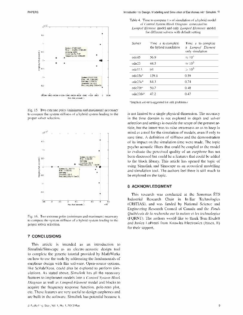
������ ����� ��� � ������� �������� ��� ��������� � ������� ���� �������� ��
���� ��� �� �� � ��� �������� ��� �������� ����� �
� ����� �� ����� �������� � � ��� �� ����� ������ � ��
� � ��� �������
���� ��� �� �� � ��� �������� ��� �������� ����� �
� ����� �� ����� �������� � � ��� �� ����� ������ � ��
� � ��� �������
� �����������
���� ����� �� ������ �� �� ���� ����� � �
��������������� �� �� ��� ��� ����� ����� �
� � ��� �� ����� ��� ��� �� ���� �� ����� ���
� � � � �� �� � � �� ��������� �� ���������� �
���� � ����� ���� ���� � ������ ����� ��� ��� ���
�� ������ � �� � �� �� � !� �� � ��� �� ����
���� ��� "� ����� �� �� ������� ��� � �� �������
������ � ������ � �� ��� � ������� ���� ��� �
������� �� � �� ����������� � � ��� � ��� �
��#��� �� ��#���� ��� �� ������ �� � �$� � ��
��� ��� ������ �� ��� ���� � ����� ���� �� ���
�� ���� �� �� � ������ ������� ��� � ����� ����� ��
���� �� ��� � ����� � � � ��������� � � ��� �� ���
� ������� ���� ��� � ������� ������ �
����������� ��� ��� ��� ����������� ���
� ���� �� ��� � ���� ������ ������
�� ��� �� � ������� ��� �� ���������
��� �� � �����
� ����� �����
��� ���������
��� ���! � �"�
�#$ ���� � �"�
���$ !� � �"�
����% �$!�& "��!
�#$�% &��$ "�'�
�#$�% �"�# "��&
�#$��% �'�# "��'
��������� ��� �������� � ���� � �����
�� � � ����� � � ���� ������� ������ �� �� ��������
�� �� ��� � ���� �� � � !� �� �� ���� ��� � ��
���� � ��� ������� �� ����� �� �� � � �� ����� ���
���� ��� �� ����� ��� � ���� ������� � �� � �� ��
���� �� � � � � �� ������� � � � ��� �� �� �� �
��� ���� " �%���� � � �������� ��� �� �� ������� �
� ��� ������ � �� ������� � ��� �� ���� �� � ���
����� ��� ����� %��� ���� � �� � � ��� � �� � �
� ����� �� ������ #����� � �� ������ ��� � �
�� �������� ��� � �� � � ������ ���� � �� � ����
� �� � �� ������� ���� ����� ��� ��� �� � ��� �
����� ������� ��� ������� �� �� �� ������ � ����
��� ������� � � � �� ���� �� � ��� �� ��� ���� �
� !� �� � �� � ����
������ ��� ��
���� ������ ��� � ������ �� �� � � ��!� &'��
(�������� )����� *���� �� (��'�� ���� ���
+*)(�("�,� ��� ��� ����� �� -��� �� ����� ���
'�������� )����� * ���� � *����� ��� �� ����
����� �� � �� � �� � �� �� ����� � � � �������
+./)-�,� �� ���� �� � �� �� � ����� � � 0�$��
��� 1���� 2 3���� �� � 4� �� '��� ���� +(������ (,
� � ���� ���� ���
�� ���� ���� � �� ��� � !� � "# $ ��% &

����� ��� ��� ���
� ����������
�� ������� �� � �� ����� ���������� � ����� ���
�� ���� ���������� �������� ����� �������� �����������
��� ���������� ��� ���� � !�
�� �� "�����#� �������� �����$���� ������% �� ��������
��������� �� ���� &�$ ��$���� &''(�
)� "��$��� ������������ ������� *���$��� ����$�� ���+
���� ,"� !$� -��.�/ ��$���� � &&�
� "�����#� ,� "��#� � �������� �� �������� � 0� ,��+
��� �� ������� �� �11� �� 2������ �� 3��.�� �� ���%�
�� *� 4����� � )�$#������ � )����$�� �� � )����$�
���������� ��� ��������� ��������� ����� ������
)������ (� ��$���� � &�
�� 5����� 5����� �� �� ���1���� ���� �� �� ����$��%+
����� �����+�1��#��� � 6�
� "� ,����� �� � �� �����%� ���1������ �� 2�$���#
�� 0���+*�� ������$����$��� �� $�� *7$����� *��� �������
� ��� ����� �� ������� �������� �&-(/8&!69&:!� &';(�
4� 4� ���$��%� ,� 3� "����� �� �� �� �����$����� �� ���� ���
������� � ������� ���� � ������� ������ ���������
�40 ����$��� ����� *������� ������� 2� ���� &�$ ��+
$���� &''<�
=�$����$����� *���$��$�������� ����������� =*� : (&6+
!8� : -������$��� �� ����� ��� �� ��� + ���$ !8 � ��(
���1��� ��� $�� ����������$ �� ������� ��� �� ���1�����
���1�� $� $�� ��� �% ����� �� ��� �����$�/� � :�
=�$����$����� *���$��$�������� ����������� =*� : (&6+
<8� & -������$��� �� ����� ��� �� ��� ���$ <8
3�����+��� ������$�� ��� $�� ����������$ �� ���1�����
���1�� $� $�� ��� �% ����� �� ��� �����$�/� � & �
� ������ � ����������������� ���������� ������ ��+
$��� 4�������� ���.����$% �� 5�����#� � '�
�� >������ "� ���� �� ������������ �� �� 2������� ���+
���$��� �� $�� =*� : ;&& ������ ��� ������$��� =� !!"��
���#������� 1���� &96� "������ 5*� � <� ���� *�������+
��� �����$%�
� ������ ��=�* ������$��� �� ���1����� �� ���1������
=� !$%�� ���#������� 1���� &9&(� 2�� ?��#� ���� � '�
���� *���������� �����$%�
*� ���%�@��� ��#����� �� ������� ����������� ���
)���% A ����� �$� ����#��� 2� ���� & $� ��$���� � & �
)� � ����� �� ���1�$�� ��� *���$��+�����$�� 5�����
��$� ��=�*� ������� � ��� ����� �� ������� ��������
('-;/8!!&9!:�� &''&�
�� ���#� 0� ,� "������ 0� )��$���� B�$@#%� �� ,� ��������
����������������� ����� �� ������������� � ���
����������� ����������& ���������� ��� ������� '���
(���& ����� )���������� ��� ������������ �1������+
C������ "������ 5*� &�$ ��$���� � &&�
2� �� 2���� ������� ����� �� ������� � ��� )���% A
����� �$� ����#��� 2� ���� :$� ��$���� � &&�
�� �� ���%� 4�� *���$����� *D��.����$ ������$ �� ������
���1����$ �������� �� 0���$� �%�$���� =� %*�� ����
#������� 1���� &9<� *����.��� 2�� &'6(� ���� *�������+
��� �����$%�
� 0����� ������ ������� ���%$�����D��� �$ ���.����$�����
0������� ��������� ��� &�$ ��$���� � ;�
*� �$��$@��� ,� ��������$� ,� �����D���� �� 2� ��������
���1������ ��$���� .��$��� �� ������$ ��.��� ��$���
�� � �����+�1��#��� ������� �������� ;(-&&/8& 6;9& '6�
2�.� � &��
�����
� ����������
+ � C����� E��F
� � ���$ ��1���$% ��$�� E� &�<F
� � 5����$% �� G�� E� &��&��
��F
� � C������$% ����H����$ E&�6:� & �� ���
��F
�� �� ����� ���� ���� ���� �� ��� �� ���� ���


BIBLIOGRAPHY
Agarwal, Anant and Jeffrey H. Lang, 2005. Foundations of Analog and Digital ElectronicCircuits. San Francisco, CA, USA : Morgan Kaufmann Publishers, 1009 p.
Algazi, V. R., R. Duda, D. M. Thompson, and C. Avendano. 2001. “ The CIPIC HRTF
Database ”. In IEEE Workshop on Applications of Signal Processing to Audio andAcoustics. (New Paltz, NY, USA 2001), p. 99–102. Institute of Electrical and Elec-
tronics Engineers.
Alten, Stanley R., 2011. Working with Audio. ed. 1st. Boston : Course Technology, Cengage
Learning, 358 p.
Atsushi, Marui and William L Martens. 2006. “ Spatial Character and Quality Assessment of
Selected Stereophonic Image Enhancements for Headphone Playback of Popular Mu-
sic ”. In 120th Convention. (Paris, FR 2006), p. 13. Audio Engineering Society.
Attia, John Okyere, 1999. ELECTRONICS and CIRCUIT ANALYSIS using MATLAB. ed. 1st.
Boca Raton, FL, USA : CRC Press LLC, 386 p.
Bauer, Benjamin B. 1961. “ Stereophonic Earphones and Binaural Loudspeakers ”. Journal ofthe Audio Engineering Society, vol. 9, n◦ 2, p. 148–151.
Bech, Søren and Nick Zacharov, 2006. Perceptual Audio Evaluation -Theory, Method andApplication. ed. 1st. Chichester : John Wiley & Sons, Ltd, 464 p.
Beranek, Leo Leroy, 1993. Acoustics. ed. 1st. Cambridge, MA, USA : Acoustical Sociery of
America, 491 p.
Berger, Elliott H. 2005. “ Preferred Methods for Measuring Hearing Protector Attenuation ”.
In The 2005 Congress and Exposition on Noise Control Engineering. (Rio De Janeiro,
BR 2005), p. 10. Institute of Noise Control Engineering.
Blau, Matthias, Tobias Sankowsty, Philipp Roeske, Hamidreza Mojallal, Magnus Teschner, and
Comelia Thiele. 2010. “ Prediction of the Sound Pressure at the Ear Drum in Occluded
Human Cadaver Ears ”. Acta Acustica united with Acustica, vol. 96, n◦ 3, p. 554–566.
Bolton, William, 2011. Mechatronics. ed. 5th (Rev.). Harlow, GB : Pearson Education Limited,
648 p.
Borwick, John, Graham Bank, Martin Colloms, Laurie Fincham, Mark R. Gander, Keith Hol-
land, Peter Mapp, Philip Newell, Sean Olive, Carl Poldy, Floyd E. Toole, John Watkin-
son, John Woodgate, and Julian Wright, 2001. Loudspeaker and Headphone Handbook.
ed. 3rd. Woburn : Focal Press, 718 p.
Bright, Andrew. 2002. “ Active Control of Loudspeakers : An Investigation of Practical Ap-
plications ”. Phd thesis, Technical University of Denmark. <http://www.elektro.dtu.dk/
English/research/publications_elektro.aspx?lg=showcommon&id=60678>, 1–203 p.
160
Brown, Andrew D and Christopher G Stecker. May 2013. “ The precedence effect: Fusion and
lateralization measures for headphone stimuli lateralized by interaural time and level
differences. ”. The Journal of the Acoustical Society of America, vol. 133, n◦ 5, p. 2883–
2898.
Brüel & Kjær. 1997. “ Wideband Ear Simulator for Telephonometry - Type 4195 ”.
Ciric, Dejan G. and Dorte Hammershøi. 2006. “ Coupling of earphones to human ears and to
standard coupler ”. The Journal of the Acoustical Society of America, vol. 120, n◦ 4, p.
2096–2107.
COMSOL Inc. 2013. “ LiveLink for MATLAB ”.
Cunningham, W J. 1949. “ Non-Linear Distortion in Dynamic Loudspeakers due to Magnetic
Effects ”. The Journal of the Acoustical Society of America, vol. 21, n◦ 3, p. 202–207.
D’Appolito, Joseph, 1998. Testing Loudspeaker. ed. 1st. Peterborough : Audio Amateur Press,
144 p.
Darlington, Paul. 1998. “ Low Frequency Modelling Using 2 Port Methods ”. In 13th UKConference: Microphones & Loudspeakers. (London, UK 1998), p. 106–112. Audio
Engineering Society.
Davis, Stanley M., 1997. Future Perfect. ed. 2nd. Reading, USA : Addison-Wesley Publishing,
272 p.
Dedieu, Stephane. 2008. “ Design of an earphone based on an electrodynamic micro-speaker ”.
Egolf, David Post, David R. Tree, and Lawrence L. Feth. 1978. “ Mathematical predictions of
electroacoustic frequency response of in situ hearing aids ”. The Journal of the Acousti-cal Society of America, vol. 63, n◦ 1, p. 264–271.
Fastl, Hugo. 1985. “ Gibt es den Frequenzgang von kofhorern? (Does the frequency response
of headphones exist?) ”. ITG-Fachberichte, p. 274–281.
Fleischmann, Felix, Andreas Silzle, and Jan Plogsties. 2012. “ Identication and Evaluation of
Target Curves for Headphones ”. In 133rd Convention. (San Francisco, Ca 2012), p.
1–11. Audio Engineering Society.
Fletcher, Harvey and W. A. Munson. 1933. “ Loudness, Its Definition, Measurement and
Calculation ”. Journal of the Acoustical Society of America, vol. 5, n◦ 1, p. 82–108.
Gabrielsson, Alf, Ulf Rosenberg, and Hakan Sjögren. April 1974. “ Judgments and dimension
analyses of perceived sound quality of sound-reproducing systems ”. The Journal of theAcoustical Society of America, vol. 55, n◦ 4, p. 854–861.
Gabrielsson, Alf, Björn Hagerman, Tommy Bech-kristensen, and Göran Lundberg. 1990.
“ Perceived sound quality of reproductions with different frequency responses and sound
levels ”. The Journal of the Acoustical Society of America, vol. 88, n◦ 3, p. 1359–1366.

161
Gardner, Mark B. and Melville S. Hawley. 1973. “ Comparison of Network and Real-Ear
Characteristics of the External Ear ”. Journal of the Audio Engineering Society, vol. 21,
n◦ 3, p. 158–165.
Gelfand, Stanley A., 2009. Essentials of Audiology. ed. 3rd. New York, NY, USA : Thieme
Medical Publishers, Inc., 560 p.
Hammershøi, D and Henrik Møller. July 1996. “ Sound transmission to and within the human
ear canal. ”. The Journal of the Acoustical Society of America, vol. 100, n◦ 1, p. 408–27.
Hartley, Tom T., Guy O. Beale, and Stephen P. Chicatelli, 1994. Digital simulation of dynamicsystems : a control theory approach. ed. 1st. Englewood Cliffs, NJ, USA : PTR Prentice
Hall, 393 p.
Hartmann, W M and A Wittenberg. June 1996. “ On the externalization of sound images. ”.
The Journal of the Acoustical Society of America, vol. 99, n◦ 6, p. 3678–3688.
Hiebel, Holger. 2012. “ Suspension Creep Models for Miniature Loudspeakers ”. In 132ndConvention. (Budapest, Hungary 2012), p. 1–5. Audio Engineering Society.
Hiipakka, Marko, Miikka Tikander, and Matti Karjalainen. 2010. “ Modeling of External Ear
Acoustics for Insert Headphone Usage ”. Journal of the Audio Engineering, vol. 58,
n◦ 4, p. 269–281.
Hodgson, Murray. 1994. “ When Is Diffuse-Field Theory Accurate? ”. Journal of the CanadianAcoustical Association, vol. 22, n◦ 3, p. 41–42.
Hudde, H and S Schmidt. May 2009. “ Sound fields in generally shaped curved ear canals. ”.
The Journal of the Acoustical Society of America, vol. 125, n◦ 5, p. 3146–57.
Inanaga, Kiyofumi, Gunnar Rasmussen Takeshi Hara, and Yasuhiro Riko. 2008. “ Research on
a measuring method of headphones and earphones using HATS ”. In 125th Convention.
(San Francisco, USA 2008), p. 1–10. Audio Engineering Society.
International Electrotechnical Commission. 2006. “ IEC 60318-5:2006 (Simulators of human
head and ear - Part 5: 2 cm3 coupler for the measurement of hearing aids and earphones
coupled to the ear by means of ear inserts) ”.
International Electrotechnical Commission. 2009. “ IEC 60318-1:2009 (Ear simulator for the
measurement of supra-aural and circumaural earphones) ”.
International Electrotechnical Commission. 2010a. “ IEC 60268-7:2010 (Sound system equip-
ment – Part 7: Headphones and earphones) ”.
International Electrotechnical Commission. 2010b. “ IEC 60318-4:2010 (Simulators of human
head and ear – Part 4: Occluded-ear simulator for the measurement of earphones coupled
to the ear by means of ear inserts) ”.
162
International Electrotechnical Commission. 2011. “ IEC 60318-7:2011 (Head and torso simu-
lator for the measurement of hearing aids) ”.
International Organization for Standardization. 1997. “ ISO 266:1997 (Preferred frequen-
cies) ”.
International Organization for Standardization. 2004. “ ISO 226:2004 (Normal equal-loudness-
level contours) ”.
Janschek, Klaus, 2012. Mechatronic systems design: methods, models, concepts. ed. 1st.
Berlin, DE : Springer-Verlag Berlin Heidelberg, 826 p.
Jardin, Audrey. 2010. “ Contribution à une méthodologie de dimensionnement des systèmes
mécatroniques : analyse structurelle et couplage à l’optimisation dynamique ”. Doctor-
ate, Institut Nationale des Sciences Appliquées de Lyon, 414 p.
Jensen, Joe. 2009. “ A balanced-armature loudspeaker model ”. Master, Technical University
of Denmark, 83 p.
Jensen, Joe, Finn T Agerkvist, and James M Harte. 2011. “ Nonlinear Time-Domain Modeling
of Balanced- Armature Receivers ”. Journal of the Audio Engineering Society, vol. 59,
n◦ 3, p. 91–101.
Jønsson, Søren, Bin Liu, Andreas Schuhmacher, and Lars Nielsen. 2004. “ Simulation of the
IEC 60711 occluded ear simulator ”. In 116th Convention. (Berlin, DE 2004), p. 1–8.
Audio Engineering Society.
Kahrs, Mark. 2009. “ SPICE simulation of headphones and earphones ”. In 127th Convention.
(New York, USA 2009), p. 1–13. Audio Engineering Society.
Karris, Steven T., 2009. Circuit Analysis II with MATLAB Computing and Simulink/SimPow-erSystems Modeling. ed. 1st. Fremont, Ca, USA : Orchard Publications, 678 p.
Keefe, Douglas H. 1984. “ Acoustical wave propagation in cylindrical ducts : Transmission
line parameter approximations for isothermal and nonisothermal boundary conditions ”.
Journal of the Acoustical Society of America, vol. 75, n◦ January, p. 58–62.
Keidser, G, R Katsch, H Dillon, and F Grant. June 2000a. “ Relative loudness perception
of low and high frequency sounds in the open and occluded ear. ”. The Journal of theAcoustical Society of America, vol. 107, n◦ 6, p. 3351–3357.
Keidser, G, R Katsch, H Dillon, and F Grant. June 2000b. “ Relative loudness perception
of low and high frequency sounds in the open and occluded ear. ”. The Journal of theAcoustical Society of America, vol. 107, n◦ 6, p. 3351–7.
Keiper, Winfried. 1997. “ Sound Quality Evaluation in the Product Cycle ”. Acustica - ActaAcustica, vol. 83, n◦ 5, p. 784–788.
163
Keith, Stephen E., David S. Michaud, Katya Feder, Ifaz Haider, Leonora Marro, Emma Thomp-
son, and Andre M. Marcoux. November 2011. “ MP3 player listening sound pressure
levels among 10 to 17 year old students. ”. The Journal of the Acoustical Society ofAmerica, vol. 130, n◦ 5, p. 2756–2764.
Killion, Mead C. 1978. “ Revised’ estimate of minimum audible pressure: Where is the "miss-
ing 6 dB"? ”. Journal of the Acoustical Society of America, vol. 63, n◦ 5, p. 1501–1508.
Klippel, Wolfgang. 2006. “ Tutorial : Loudspeaker Nonlinearities — Causes , Parameters ,
Symptoms ”. Journal of the Audio Engineering Society, vol. 54, n◦ 10, p. 907–939.
Klippel, Wolfgang and Joachim Schlechter. 2006. “ Measurement and Visualization of Loud-
speaker Cone Vibration ”.
Kreyszig, Erwin, 2010. Advanced Engineering Mathematics. ed. 10th. Hoboken, NJ, USA :
John Wiley & Sons, Ltd, 1280 p.
Leach Jr., William Marshall. 1991. “ Computer Aided Electro-Acoustic Design with SPICE ”.
Journal of the Audio Engineering Society, vol. 39, n◦ 7, p. 551–562.
Leach Jr., William Marshall, 2010. Introduction to Electroacoustics and Audio AmplifiersDesign. ed. 4th. Dubuque : KendallL/Hunt Publishing Company, 293 p.
Lenk, Arno, Rüdiger G. Ballas, Roland Werthschützky, and Günther Pfeifer, 2011. Electrome-chanical Systems in Microtechnology and Mechatronics: Electrical, Mechanical andAcoustic Networks, their Interactions and Applications. ed. 1st. Berlin, DE : Springer-
Verlag, 482 p.
Letowski, Tomasz. 1989. “ Sound Quality Assessment: Concepts and Criteria ”. In 87thConvention. (New York, USA 1989), p. 12. Audio Engineering Society.
Litovsky, R Y, H S Colburn, W a Yost, and S J Guzman. October 1999. “ The precedence
effect. ”. The Journal of the Acoustical Society of America, vol. 106, n◦ 4 Pt 1, p. 1633–
54.
Lorho, Gaëtan. 2005. “ Evaluation of Spatial Enhancement Systems for Stereo Headphone
Reproduction by Preference and Attribute Rating ”. In 118th Convention. (Barcelona,
ES 2005), p. 20. Audio Engineering Society.
Lorho, Gaëtan. 2009. “ Subjective Evaluation of Headphone Target Frequency Responses ”. In
126th Convention. (Munich, DE 2009), p. 1–20. Audio Engineering Society.
Mapes-Riordan, Dan. 1993. “ Horn Modeling with Conical and Cylindrical Transmission-Line
Elements ”. Journal of the Audio Engineering Society, vol. 41, n◦ 6, p. 471–484.
Mehrgardt, S and V. Mellert. 1977. “ Transformation Characteristics of the External Human
Ear ”. Journal of the Acoustical Society of America, vol. 61, n◦ 6, p. 1567–1576.

164
Merriam-Webster, 1998. Merriam-Webster’s Collegiate Dictionnary. ed. 10th. Springfield,
MA, USA : Merriam-Webster, Inc., 1562 p.
Møller, Henrik, Dorte Hammershøi, Jorn Vagn Hunderboll, and Clemen Boje Jensen. 1992.
“ Transfer Characteristics of Headphones: Measurements on 40 Human Subjects ”. In
92nd Convention. (Vienna 1992), p. 1–29. Audio Engineering Society.
Møller, Henrik, Clemen Boje Jensen, Dorte Hammershøi, and Michael Friis Sørensen. 1995a.
“ Design Criteria for Headphones ”. Journal of the Audio Engineering Society, vol. 43,
n◦ 4, p. 1–15.
Møller, Henrik, Michael Friis Sørensen, Dorte Hammershøi, and Clemen Boje Jensen. 1995b.
“ Head-Related Transfer Functions of Human Subjects ”. Journal of the Audio Engineer-ing Society, vol. 43, n◦ 5, p. 300–321.
Moore, Brian C. J., Brian R. Glasberg, and Thomas Baer. 1997. “ A Model for the Prediction
of Thresholds, Loudness, and Partial Loudness ”. Journal of the Audio Engineering,
vol. 45, n◦ 4, p. 224–240.
Morgan, Donald E and Donald D Dirks. 1974. “ Loudness discomfort level under earphone and
in the free field : methods ”. The Journal of the Acoustical Society of America, vol. 56,
n◦ 1, p. 172–178.
Nadol Jr., Joseph B. and Michael J. McKenna, 2005. Surgery of the Ear and Temporal Bone.
ed. 2nd. Philadephia, PA, USA : Lippincott Williams & Wilkins, 608 p.
Nise, Norman S., 2011. Control Systems Engineering. ed. 6th. Hoboken, NJ, USA : John
Wiley & Sons, Ltd, 926 p.
NPD Group. 2012. “ NPD Group : Headphones Priced at Above Account for More than $340
Million in Sales Through November ”.
Oksanen, Sami, Marko Hiipakka, and Ville Sivonen. 2012. “ Estimating individual sound
pressure levels at the eardrum in music playback over insert headphones ”. In 47thInternational Conference. (Chicago, IL, USA 2012), p. 1–8. Audio Engineering Society.
Olive, Sean E and Todd Welti. 2012a. “ The Relationship between Perception and Measurement
of Headphone Sound Quality ”. In 133rd Convention. (San Francisco 2012), p. 1–17.
Audio Engineering Society.
Olive, Sean E and Todd Welti. 2012b. “ The Relationship between Perception and Measure-
ment of Headphone Sound Quality ”. In 133rd Convention. (San Francisco 2012), p.
1–42. Audio Engineering Society;.
Olive, Sean E, Todd Welti, and Elisabeth Mcmullin. 2013. “ Listener Preference For Different
Headphone Target Response Curves ”. In 134th Convention. (Rome, IT 2013), p. 12.
Audio Engineering Society.

165
Poldy, Carl A. 1983a. “ The Electrical Equivalent Circuit of Porous Compliant Membranes
and Related Systems ”. In 73rd Convention. (Eindhover, NL 1983), p. 1–4. Audio
Engineering Society.
Poldy, Carl A. 1983b. “ Electrical Analogs for Membranes with ApplicatIon to Earphones ”.
Journal of the Audio Engineering, vol. 31, n◦ 11, p. 817–825.
Poldy, Carl A. 2006. “ Headphone fundamentals ”. In Pro Audio Expo & Convention. (Paris
2006), p. 1–57. Audio Engineering Society.
Post, John Theodore. 1994. “ A modeling and measurement study of acoustic horns ”. Doctor-
ate, University of Texas at Austin, 192 p.
Pralong, Danièle and Simon Carlile. December 1996. “ The role of individualized headphone
calibration for the generation of high fidelity virtual auditory space. ”. The Journal ofthe Acoustical Society of America, vol. 100, n◦ 6, p. 3785–93.
Robinson, D. W. and R. S. Dadson. 1956. “ A re-determination of the equal-loudness relations
for pure tones ”. British Journal of Applied Physics, vol. 7, n◦ 5, p. 166–181.
Rossi, Mario, 2007. Audio. ed. 1st. Lausanne, CH : Presses Polytechniques et Universitaires
Romandes, 753 p.
Sakamoto, N, T Gotoh, and Y Kimura. 1976. “ On " Out-of-Head Headphone Localization "
Listening ”. Journal of the Audio Engineering Society, vol. 24, n◦ 9, p. 710–716.
Salmon, Vincent. 1944. “ Acoustic Horn ”.
Schönstein, David and Brian F G Katz. 2010. “ Variability in perceptual evaluation of HRTFs ”.
In 128th Convention. (London, UK 2010), p. 11. Audio Engineering Society.
Scilab Enterprises S.A.S. 2013. “ Scilab/Xcos ”. <http://www.scilab.org/en>.
Shiah, Y C, Hong-ching Her, Jin H. Huang, and Brant Huang. 2008. “ Parametric analysis for
a miniature loudspeaker used in cellular phones ”. Journal of Applied Physics, vol. 104,
n◦ 10, p. 104905–1 104905–10.
Shimokura, Ryota and Yoshiharu Soeta. September 2012. “ Listening level of music through
headphones in train car noise environments. ”. The Journal of the Acoustical Society ofAmerica, vol. 132, n◦ 3, p. 1407–1416.
Struck, Christopher J. 1987. Determination of the Thiele - Small Parameters Using Two-Channel FFT Analysis. Technical Report 1. Hoffman Estates, IL : Brüel & Kjaer, 1–6 p.
Sturtzer, E., G. Pillonnet, G. Lemarquand, and N. Abouchi. November 2012. “ Comparison
between voltage and current driving methods of a micro-speaker ”. Applied Acoustics,
vol. 73, n◦ 11, p. 1087–1098.
166
Takemoto, Hironori, Parham Mokhtari, Hiroaki Kato, Ryouichi Nishimura, and Kazuhiro Iida.
December 2012. “ Mechanism for generating peaks and notches of head-related transfer
functions in the median plane. ”. The Journal of the Acoustical Society of America, vol.
132, n◦ 6, p. 3832–41.
Temme, Steve, Pascal Brunet, and D. B. Keele Jr. 2009. “ Practical Measurement of Loud-
speaker Distortion Using a Simplified Auditory Perceptual Model ”. In 127th Conven-tion. (New York, USA 2009), p. 1–17. Audio Engineering Society.
Temme, Steve, Pascal Brunet, and Parastoo Qarabaqi. 2012. “ Measurement of Harmonic
Distortion Audibility Using a Simplified Psychoacoustic Model ”. In 133rd Convention.
(San Francisco 2012), p. 1–9. Audio Engineering Society.
The Mathworks Inc. 2013. “ MATLAB/Simulink ”. <http://www.mathworks.com/index.html>.
Theile, Günther. 1986. “ On the Standardization of the Frequency Response of High-Quality
Studio Headphones ”. Journal of the Audio Engineering Society, vol. 34, n◦ 12, p. 956–
969.
Thurstone, LL. 1927. “ A law of comparative judgment ”. Psychological review, vol. 34, p.
273–286.
Toole, Floyd E. 1984. “ The Acoustics and Psychoacoustics of Headphones ”. In The Art andTechnology of Recording. (Anaheim 1984), p. 15. Audio Engineering Society.
Toole, Floyd E., 2008. Sound Reproduction. ed. 1st. Burlington, MA, USA : Focal Press,
569 p.
Valente, Michael, Lisa G. Potts, Maureen Valente, William Vass, and Joel Goebel. 1994.
“ Intersubject variability of real-ear sound pressure level: Conventional and insert ear-
phones ”. Journal of the American Academy of Audiology, vol. 5, n◦ 6, p. 390–398.
Vanderkooy, John and Kevin B Krauel. 2012. “ Another View of Distortion Perception ”. In
133rd Convention. (San Francisco 2012), p. 1–4. Audio Engineering Society.
Villchur, E. December 1969. “ Free-field calibration of earphones. ”. The Journal of theAcoustical Society of America, vol. 46, n◦ 6, p. 1527–1534.
Villchur, Edgar Marion. 1957. “ Problems of Bass Reproduction in Loudspeakers ”. Journalof the Audio Engineering Society, vol. 5, n◦ 3, p. 122–126.
Vitt, Nikolas T. 2011. “ Investigation of a Balanced-Armature Transducer for Vibrational
Energy Harvesting ”. Master, Pennsylvania State University, 127 p.
Voix, Jérémie, Cécile Le Cocq, and Lee D. Hager. 2008. “ The Healthy Benefits of Isolating
Earphones ”. In Session 3pPPb: Psychological and Physiological Acoustics. (Paris, FR
2008), p. 050003–050003. Acoustical Society of America.
167
Völk, Florian and Hugo Fastl. 2011. “ Locating the Missing 6 dB by Loudness Calibration of
Binaural Synthesis ”. In 131st Convention. (New York 2011), p. 1–12. Audio Engineer-
ing Society.
White, James V. 1963. “ Considerations in High-Fidelity Moving-Coil Earphone Design ”.
IEEE Transactions on Audio, vol. 11, n◦ 6, p. 188–194.
Zuercher, Joseph C., Elmer V. Carlson, and Mead C. Killion. 1988. “ Small acoustic tubes
: New approximations including isothermal and viscous effects ”. The Journal of theAcoustical Society of America, vol. 83, n◦ 4, p. 1653–1660.
Zwicker, Eberhard and Hugo Fastl, 2007. Psycho-Acoustics: Facts and Models. ed. 3rd. Berlin,
DE : Springer-Verlag Berlin Heidelberg, 462 p.