cold water diving for science - welcome to the national sea grant
TRANSCRIPT

Cold Water Diving for Science
Stephen C. Jewett, Editor
American Academy of Underwater SciencesProceedings of the 21st Annual
Scientific Diving Symposium
September 19-23, 2001Alaska Sea Life CenterSeward, Alaska
Published by University of Alaska Sea GrantFairbanks, AlaskaAK-SG-01-06

Elmer E. Rasmusen Library Cataloging-in-Publication Data
Scientific Diving Symposium (21st : 2001 : Seward, Alaska)Cold water diving for science : American Academy of Underwater Sciences21st annual Scientific Diving Symposium, September 19-23, 2001, Seward,Alaska / Stephen C. Jewett, editor. – Fairbanks, Alaska : University of Alaska Sea Grant, [2001].
104 p. : ill. ; cm. – (University of Alaska Sea Grant College Program ; AK-SG-01-06)
Includes bibliographical references.
1. Scuba diving—Congresses. 2. Oceanographic submersibles—Congress-es. 3. Submersibles—Congresses. 4. Remote submersibles—Congresses.5. Underwater physiology—Congresses. I. Title. II. Jewett, Stephen C. III.Series: Alaska Sea Grant College Program report ; AK-SG-01-06. IV. Ameri-can Academy of Underwater Sciences.
QH90.57.S38 S35 2001
ISBN 1-56612-069-1
AcknowledgmentsThis book is published by the University of Alaska Sea Grant College Program,which is cooperatively supported by the U.S. Department of Commerce, NOAANational Sea Grant Office, grant no. NA86RG-0050, project A/161-01; and by theUniversity of Alaska Fairbanks with state funds. The University of Alaska is anaffirmative action/equal opportunity institution.
Sea Grant is a unique partnership with public and private sectors combiningresearch, education, and technology transfer for public service. This national net-work of universities meets changing environmental and economic needs of peoplein our coastal, ocean, and Great Lakes regions.
University of Alaska Sea GrantP.O. Box 755040203 O’Neill Bldg.Fairbanks, Alaska 99775-5040(888) 789-0090 (toll free)Fax (907) 474-6285http://www.uaf.edu/seagrant/
Citation for this book is:
S.C. Jewett (ed.). 2001. Cold Water Diving for Science. Proceedings of the21st Annual Scientific Diving Symposium, American Academy of Under-water Sciences. University of Alaska Sea Grant, AK-SG-01-06, Fairbanks.

Table of Contents
PrefaceS.C. Jewett .......................................................................................................... v
German Activity in Cold Water Scientific DivingB. Bluhm, K. Iken, J. Laudien, and H. Lippert ...................................................... 1
An Experiment of Simulated Predation: Can River Otters BecomeFood Limited in a Marine System?G.B. Blundell, S.C. Jewett, T.A. Dean, and R.T. Bowyer ........................................ 5
Survey Design and Methods for Determining Oil Spill Damageto Pacific Herring (Clupea pallasi) EmbryosE.D. Brown ........................................................................................................ 11
Diving Techniques Used for Deploying an Underwater CameraArray During Sonar Operation in the Chandalar River, AlaskaE.J. Brown and B.M. Osborne ............................................................................ 15
Investigation of the Overwintering of the Annual MacroalgaNereocystis luetkeana in Kachemak Bay, AlaskaH. Chenelot, J. Matweyou, and B. Konar ........................................................... 19
West Florida Continental Shelf: Diving and the ECOHAB-ONR-COMPS Monitoring ArrayR. Cole .............................................................................................................. 25
A Comparison of Tethered Research Diving in Lake Hoare,Taylor Valley, Antarctica, Using a Surface-Supplied Air Sourceand ScubaR.R. Costello and P.T. Doran .............................................................................. 27
Transplanting Giant Kelp (Macrocystis pyrifera) onto ArtificialReefs: The San Clemente Reef Mitigation ProjectT.A. Dean and D. Jung ....................................................................................... 31
El Niño 1997-1998: Large-Scale Patterns of Disturbance andRecovery in Giant Kelp ForestsM.S. Edwards .................................................................................................... 35
iv
Red Sea Urchin Growth in Southeast AlaskaK.P. Hebert and D.A. Woodby ............................................................................ 39
Scuba Techniques Used to Assess the Effects of theExxon Valdez Oil SpillS.C. Jewett, T.A. Dean, and M. Hoberg .............................................................. 43
Underwater Capture of Juvenile Steller Sea Lions with Scuba: ANarrated Video PresentationD.C. McAllister, D.G. Calkins, and K.W. Pitcher ................................................. 53
Photosynthetic Response of Arctic Kelp Forests to StratosphericOzone DepletionH.L. Miller III and K.H. Dunton.......................................................................... 57
A Year in the Life of a Piling: Recruitment of King Crabs and OtherFauna to Dock PilingsE. Munk, B. Stevens, and P. Cummiskey ............................................................ 63
Development of Virtual Field Trips/Site Briefingsfor the InternetS.F. Norton ........................................................................................................ 65
Movement Patterns of the Chiton Katharina tunicata inKachemak Bay, AlaskaJ. Plett and B. Konar ......................................................................................... 71
Scientific Diving Injuries in Southeast AlaskaM. Pritchett ....................................................................................................... 75
A Mountain in the Sea: Exploration of a Gulf of Alaska Seamountwith the Submersible AlvinB. Stevens ......................................................................................................... 79
Voyage to See What’s on the Bottom: Methods ofVisualizing the Ocean FloorB. Stevens ......................................................................................................... 81
Jellyfish Effects on Food Web Production in the Bering SeaS. Whitney ......................................................................................................... 89
A Fisheries Habitat Survey Method for Nearshore EnvironmentsUtilizing ScubaE.J. Maney Jr., and C. McMannus ...................................................................... 93
Hyperpycnal Plumes in Shelf Waters of the Exuma Cays, Bahamas:A Trigger for Coral Bleaching?P.A. Pitts ............................................................................................................ 95

v
PrefaceStephen C. JewettThese proceedings contain 22 extended abstracts of papers presented be-fore Cold Water Diving for Science, the 21st Annual Scientific Diving Sym-posium sponsored by the American Academy of Underwater Sciences. Thesymposium was held September 19-23, 2001, at the Alaska SeaLife Centerin Seward, Alaska. The first part of the program, a technical forum on coldwater diving, enabled several invited experts in the field to share theirknowledge and experience, to result in another AAUS scientific diving re-source document Cold Water Diving for Science: Tips, Techniques andTraining, a post-symposium publication. The second part of the program,these proceedings, included a variety of interdisciplinary presentations,most relevant to cold water diving.
This is the third AAUS proceedings to focus on cold water diving forscience. The first was Coldwater Diving for Science 1987 (Michael A. Lang,Editor), held at the University of Washington. It resulted in Special Sessionon Coldwater Diving (Michael A. Lang and Charles T. Mitchell, editors) aswell as the regular proceedings. The second proceedings was the AAUSPolar Diving Workshop (Michael A. Lang and James R. Stewart, editors),held at Scripps Institution of Oceanography in May 1991. The rationale forrevisiting cold water diving for science is to update the scientific divingcommunity on recent advances made in gear, techniques, and trainingnecessary to conduct research in such an extreme environment.
The symposium was hosted by the Alaska SeaLife Center; Prince Will-iam Sound Science Center; Alaska Underwater Science Foundation; andthe University of Alaska Fairbanks School of Fisheries and Ocean Sciences,Scientific Diving Program, and West Coast and Polar Regions UnderseaResearch Center. The steering committee consisted of Robert Hicks (chair),Tom Kline, Val Hodges, and Stephen Jewett. Thanks to the following formaking these proceedings possible: the authors for contributing manu-scripts; Sue Mitchell for copy editing and layout; Tatiana Piatanova fordesigning the cover; John N. Heine for cover photo (McMurdo Station,Antarctica); Sue Keller for proofreading; and University of Alaska Sea Grantfor publishing.

vi
AUSF
Alaska UnderwaterScience Foundation
West Coast & Polar RegionsUndersea Research Center

Cold Water Diving for Science 1University of Alaska Sea Grant • AK-SG-01-06, 2001
German Activity inCold Water Scientific DivingBodil A. Bluhm1315 Spring Glade Rd., Fairbanks, AK 99709, 907-474-7407 (tel.),907-474-7204 (fax), [email protected]
Katrin IkenDept. of Biology, University of Alabama at Birmingham, 1300 UniversityBoulevard, Birmingham, AL 35294-1170
Jürgen Laudien and Heike LippertAlfred Wegener Institute for Polar and Marine Research, Columbusstrasse,27515 Bremerhaven, Germany
The goal of this presentation is to give a brief overview of German activityin cold water scientific diving. First, we will outline the requirements forscientific diving under German legislation. Second, two locations wheremuch of the cold water diving is performed will be described, Kongsfjordin Spitsbergen (Arctic) and Potter Cove at King George Island (Antarctic).Some examples of scientific projects will be presented.
Research Diving in GermanyDiving for science in Germany goes back to the 1960s, when there were noregulations or defined requirements. After two deadly accidents in 1969,guidelines for scientific diving, modified from the “Guidelines to avoiddive accidents” applied to commercial divers, were implemented by thecivil engineering trade association (Fachausschuss Tiefbau der BGZ 1988).They define the type and characteristics of the gear, training requirements,protocols on dives and planning, and provide the legal background. Onlyafter passing an exam taken with the technical committee of the civil engi-neering trade association are divers authorized to conduct any officialresearch diving with German universities, research institutes, or any gov-ernmental organization. For every project, a contract is made between thecontracting institute and the research diver hired to do the work. Since1970, eight facilities (seven research institutes and one private company)

have obtained legal permission to provide the training. Typically, thesefacilities offer one course per year for up to twelve candidates each, mostof whom are students and technicians in biology, geology, paleontology,and archeology. Up to now (April 1, 2001), 936 divers have been certifiedas scientific divers.
As prerequisites, candidates are required to have a thorough dive phys-ical, current first aid certification including CPR, and a recent lifeguardcertification. The training comprises 240 hours in total which are typical-ly split into two parts of three to four weeks each. Five sections are cov-ered: (1) safety instructions (12 hours), (2) dive medicine (16 hours, lecturesand hands-on training), (3) gear instructions (24 hours), (4) dive duty (138hours), and (5) dives (20 hours pool, 20 hours open water up to 10 m, 10hours open water up to 30 m).
Some of the most obvious differences between diving in Germany andthe United States are that a German dive group consists of one diver in thewater who is, via a tether, directed and monitored by a dive tender on-board/on land while a standby diver and a dive operation leader are onsite. Diving is performed with a full face mask and in dry suits, thereforea buoyancy control device is not compulsory with a neoprene dry suit.
Similar to the United States, German scientific divers usually performonly non-decompression dives.
Diving in the ArcticThe base for most of the German research diving activity in the Arctic isthe Koldewey Station (established in 1991), Kongsfjord, Spitsbergen, whichis run by the Alfred Wegener Institute for Polar and Marine Research, Bremer-haven (www.awi-bremerhaven.de). The station is situated at 78.9º N, 11.9º Ewithin an international research base at Ny-Ålesund, administrated byNorway. It offers accommodation for up to eight guests; additional ac-commodation can be rented with the Norwegian Polar Institute.
Atmospheric research was the main aim when Koldewey Station wasestablished, but marine biological activities have become another majorfocus in recent years (www.awi-bremerhaven.de/Polar/koldewey.html). Thestation itself houses a chemistry lab and office facilities, whereas a ma-rine biology wet lab is rented for the summer months from the NorwegianPolar Institute. New international marine laboratory facilities are current-ly planned. In terms of dive equipment, the Koldewey Station providestwo inflatable boats. A portable compressor (200 and 300 bar) is rentedfrom the Norwegian Polar Institute; dive gear and an emergency oxygenunit are brought by the scientific dive group. At present, the closest de-compression chamber is in Tromsø (northern Norway), but a treatmentdecompression chamber will be purchased in the near future (shared amongall stations in the research community).
The Kongsfjord is an 8 km wide and 26 km long fjord with a maximumdepth of 400 m. The range of the semidiurnal tides is between 1.5 and 2 m
2 Bluhm et al. — German Activity in Cold Water Scientific Diving

2001 Cold Water Diving for Science 3
with weak currents, allowing dive activities at any time. The shores com-prise steep rocky bottom, in parts densely populated by a rich macroalgalcommunity, as well as weakly declining slopes with predominantly softglacial sediments. The input of terrestrial sediments and freshwater byglacier runoffs can reduce visibility from 20 m down to 1 m from July toSeptember. Ice cover and glacier calving can preclude diving in the innerfjord until mid-June. The mean annual water temperature is just above 0ºC but can rise to 6º C at the surface and 3.6º C at 20 m depth in summer.Over the last years, diving has taken place from early May through Sep-tember at depths of 4 to 30 m. Most sites can be reached in 15-40 min boatrides. Due to the regular occurrence of polar bears, a gun is always re-quired when a person is leaving the station.
Diving in the AntarcticIn January 1994, the Instituto Antártico Argentino and the Alfred WegenerInstitute for Polar and Marine Research established the Dallmann Labora-tory at the Argentine Jubany Station on King George Island (62º 14′S, 58º40′W), situated at Potter Cove. The Dallmann Lab is open from Octoberthrough March (Jubany Station is staffed all year round) and offers spacefor twelve people (www.awi-bremerhaven.de/Polar/dallmann.html). It isequipped with four laboratories, workshops, storage space, aquarium con-tainer, and diving equipment (including a compressor and a one-persontransportation decompression chamber). Several inflatable boats and alarger fiberglass boat are available for dive operations. Often, joint Argen-tine-German diving operations are carried out under the agreement thatthe stricter rules from either the German scientific or the Argentine pro-fessional diving regulations concerning depth and dive time are applied.
Potter Cove covers about 6 km2 and is up to 90 m deep in the outerand 50 m in the inner cove. The outer shores of Potter Cove consist ofrocky bottom with dense macroalgal cover. The southeast coast is charac-terized by a broad rocky intertidal platform connecting to a weakly de-clining sublittoral. The inner cove is predominately soft bottom composedof the sediment load provided by bordering glaciers and glacial creeks.Sometimes this freshwater inflow creates a surface layer of reduced salin-ity loaded with sediments, which significantly reduces light penetrationinto the water column below (where visibility can still be 20 m). Tempera-ture ranges from –0.9º C to 1.4º C. The cove is usually ice-covered fromMay to October.

Recent and Ongoing Projects Performed byGerman Scientific DiversKongsfjord
• UV-effects on marine macroalgae, morphological, physiological andbiochemical adaptation (e.g. Hanelt et al. 2001, and ongoing)
• Macrofauna associated with macroalgae (e.g. Lippert et al. in press)
• Plant-animal interaction between marine macroalgae and inverte-brates, with emphasis on antifeeding strategies (Hagen, Wessels;ongoing)
• Animal-animal interaction between marine invertebrates, chemicalecology (Lippert, ongoing)
Potter Cove• Macroalgal communities (e.g., Klöser et al. 1994)
• Interactions between macroalgae and herbivores (e.g., Iken 1999)
• Energy budgets of benthic suspension feeding animals of the PotterCove (e.g., Kowalke 2000)
• The function of macroalgal derived MAAs in invertebrate protectionagainst UV and antioxidative stress (Abele, Obermüller; ongoing)
ReferencesFachausschuss Tiefbau der BGZ. 1988. ZH1/540, Richtlinien fuer den Einsatz von
Forschungstauchern. Hauptverband der gewerblichen Berufsgenossenschaften,48 pp.
Hanelt, D., H. Tüg, K. Bischof, C. Groß, H. Lippert, T. Sawall, and C. Wiencke. 2001.Light regime in an Arctic fjord: A study related to stratospheric ozone deple-tion as a basis for determination of UV effects on algal growth. Mar. Biol.138:649-658.
Iken, K. 1999. Feeding ecology of the Antarctic herbivorous gastropod Laevila-cunaria antarctica Martens. J. Exp. Mar. Biol. Ecol. 236:133-148.
Klöser, H., G. Mercuri, F. Laturnus, M.L. Quartino, and C. Wiencke. 1994. On thecompetitive balance of macroalgae at Potter Cove (King George Island, SouthShetlands). Polar Biol. 14:11-16.
Kowalke, J. 2000. Ecology and energetics of two Antarctic sponges. J. Exp. Mar. Biol.Ecol. 147:85-97.
Lippert, H., K. Iken, E. Rachor, and C. Wiencke. In press. Macrofauna associatedwith macroalgae at Kongsfjord (Spitsbergen). Polar Biol.
4 Bluhm et al. — German Activity in Cold Water Scientific Diving

Cold Water Diving for Science 5University of Alaska Sea Grant • AK-SG-01-06, 2001
An Experiment of SimulatedPredation: Can River OttersBecome Food Limitedin a Marine System?Gail M. BlundellInstitute of Arctic Biology, Alaska Cooperative Fish and Wildlife ResearchUnit and Department of Biology and Wildlife, University of AlaskaFairbanks, Fairbanks, AK 99775-7000, 907-479-4331 (tel.), [email protected]
Stephen C. JewettInstitute of Marine Science, University of Alaska Fairbanks, P.O. Box757220, Fairbanks, AK 99775-7220
Thomas A. DeanCoastal Resources Associates, Inc., 1185 Park Center Drive, Suite A,Vista, CA 92083
R. Terry BowyerInstitute of Arctic Biology, and Department of Biology and Wildlife,University of Alaska Fairbanks, P.O. Box 757000, Fairbanks, AK 99775
IntroductionRiver otters (Lontra canadensis) inhabiting marine environments feed pri-marily on intertidal and demersal fishes in the nearshore system (Larsen1984, Bowyer et al. 1994). Investigations were conducted from 1995 to1998 in Prince William Sound, Alaska, to determine whether river ottersand three other top predators inhabiting the nearshore environment con-tinued to be negatively influenced by chronic effects from the 1989 ExxonValdez oil spill. That ecosystem study (Nearshore Vertebrate Predator [NVP]project) addressed the questions: Have these species recovered? If not, isit oil, or is it food? (Holland-Bartels 1999). In that study, densities of inter-tidal and demersal fishes that are commonly consumed by river otterswere compared between oiled and nonoiled sites and between randomsites and latrines used by river otters (Holland-Bartels 1999).

In this companion study, a manipulative experiment was conductedto ask the question: Can river otters affect their prey base (i.e., can river ottersbecome food limited in a marine system)? Previous studies investigatingpredator-prey interactions of Eurasian otters (Lutra lutra) and fishes (Koopand Gibson 1991; Kruuk et al. 1988) conducted experiments removingfishes (Pholis gunnellus, Zoarces viviparus, and Ciliata mustela) from studyplots by collecting fishes from under rocks and vegetation at low tide,when only a few centimeters of water remained. Both studies noted thatremoved fishes were replaced within two tidal cycles by new fishes, con-cluding that predators likely could not deplete an area of those species offishes. Those studies were limited to assessing only fishes that seek ref-uge under rocks and vegetation as the tide recedes and therefore did notevaluate potential effects of predation on all types of fishes consumed byotters.
MethodsWe used scuba equipment to conduct a fish removal experiment in
Herring Bay (oiled site) from late July to mid-August 1997, to test thehypothesis that otter predation influences local abundance of fishes. Threeremoval and three control sites with similar aspects and intertidal sub-strate characteristics were selected for the experiment. Prior to removalexperiments, demersal fishes were counted at each site along two transectsseparated by 20 m, running perpendicular to shore. Transects extended adistance of 30 m or to a depth of 15 m, whichever occurred first. Each sitewas permanently marked with 6 mm nylon rope delineating the centrallylocated 30 m transects (i.e., a 20 m wide by 30 m long area) and a bufferzone on either side of the transects (15 m wide by 30 m long).
At each transect, fish in the water column were counted over a 2 mwide swath along the bottom and a second diver moved aside vegetationand counted benthic fishes in a 1 m wide swath. All fishes were identifiedto family and classified into three size categories (<8 cm, 8-15 cm, >15cm). Following preremoval assessment of fish abundance at all sites, in-tense localized predation was simulated at removal sites by divers at-tempting to spear and remove all fishes. Four divers conducted fishremovals at each removal site on three consecutive days. Two divers wereassigned to the central 30 by 20 m area and a single diver to each of theouter areas. Each diver conducted a systematic search of the area attempt-ing to spear any fish >8 cm in length that was encountered. Spearing epi-sodes lasted 25-68 minutes. Immediately upon surfacing, divers recordedthe number of fish seen but not successfully speared (i.e. number of fishmissed) by fish family and size category (8-15 cm and >15 cm). Fish spearedduring the removal experiments were preserved in 10% buffered formalinfor P4501A1 analysis.
Censuses of central areas were conducted to assess post-removal in-fluences of simulated predation because the number of fishes encoun-
6 Blundell et al. — An Experiment of Simulated Predation

2001 Cold Water Diving for Science 7
tered on preremoval transects was few compared with the number of fish-es removed. Two days after the fish removals were completed, a censuswas done on the central 30 by 20 m area of each removal and control site,counting all demersal and pelagic fishes encountered. Censuses were re-peated at each site two weeks later. Census dives involved a systematicsearch of the entire area and required 53-82 minutes to complete, de-pending on the amount of vegetation.
Fish removal data were analyzed using paired sample t-tests and GLMrepeated measures analyses employing SAS software. Models were basedon type (removal or control) because there were insufficient degrees offreedom to run models by site. Paired t-tests conducted on preremovaltransects detected no difference between control and removal sites in fishabundance (F = 16.69, P = 0.07) thus sites were appropriate for compari-son of post-removal abundance of fishes. Significantly more fishes (>8cm) were missed than were removed (F = 7.18, P = 0.04), with greaternumbers of fishes missed and removed on each subsequent day of theexperiment (Figure 1). Divers likely acquired a better search image forfishes as the experiment progressed, and fishes likely became more cau-tious when divers were present as a result of previous experience.
A GLM repeated-measures analysis of post-removal censuses detect-ed no difference between removal and control sites in number of fishes >8cm present at each census (F = 0.06, P = 0. 824). There was, however, adifference in fish abundance between sampling events (F = 248.44, P =0.04), with a greater number of fishes present in the first post-removalcensus compared with the second census (Figure 2). By fish family (>8cm), only sculpin differed significantly between removal and control sites(greater at control sites; F = 289.0, P = 0.037), whereas cod (greater in rep#1; F = 497.03, P = 0.028) and Pricklebacks (Stichaeidae) (greater in rep #2;F = 99999.9, P < 0.001) differed significantly between census repetitions(Figure 2).
Most differences in fish abundance occurred between sampling eventsrather than between control and removal sites, indicating a seasonal fluc-tuation in fish abundance that likely was not related to the removal exper-iment. The change in abundance for all fishes >8 cm between post-removalsampling periods (Figure 2) was driven primarily by cod, which were nottargeted for removal. Preliminary food habit data obtained in 1996 from25 samples of otter feces collected from latrine sites in Jackpot and Her-ring bays indicated that cod were not an important prey item for riverotters at those sites (Holland-Bartels 1997). Pricklebacks also varied inabundance between post-removal censuses (Figure 2) and were present ingreater numbers at removal sites compared to control sites.
Only sculpin occurred in lower numbers at removal sites comparedwith control sites during post-removal sampling, indicating that these rel-atively sedate fishes, which are commonly consumed by river otters (Larsen1984, Holland-Bartels 1997), may be affected by predation. Nonetheless,when abundance of all fishes was considered, there was no difference

Figure 2. Mean number of fishes occurring at removal and control sites two days(removal and control 1) and two weeks (removal and control 2) afterremoval of fishes was conducted.
Figure 1. Total number of fishes >8 cm missed and removed at fish removal sites(n = 3) on three successive days of spearing by divers.
0
5
10
15
20
25
30
35
40
45
50
Nu
mb
er
of
Fis
he
s >
8 c
m
Mis
se
d 1
Re
mo
ve
d 1
Mis
se
d 2
Re
mo
ve
d 2
Mis
se
d 3
Re
mo
ve
d 3
Greenling
Gunnels
Pricklebacks
Ronquils
Sculpin
8 Blundell et al. — An Experiment of Simulated Predation
Removal 1 Control 1 Removal 2 Control 20
5
10
15
20
25
30
35
40
Sculpin
Greenling
Gunnels
Pricklebacks
Ronquils
Me
an
nu
mb
er
of
fish
es

2001 Cold Water Diving for Science 9
between removal and control sites in post-removal abundance of fishes>8 cm, indicating that the removal of fishes at those sites did not affectthe subsequent number of most fish species that were present. Our con-clusions agree with those of previous otter-fish studies (Koop and Gibson1991; Kruuk et al. 1988). Because of the mobility of most demersal fishes,prey removed by predators are quickly replaced and depletion of a site isunlikely when fishes occur at densities similar to those noted during thisstudy.
ReferencesBowyer, R.T., J.W. Testa, J.B. Faro, C.C. Schwartz, and J.B. Browning. 1994. Changes
in diets of river otters in Prince William Sound, Alaska: Effects of the ExxonValdez oil spill. Can. J. Zool. 72:970-976.
Holland-Bartels, L. (ed.). 1997. Mechanisms of impact and potential recovery ofnearshore vertebrate predators. Exxon Valdez oil spill restoration report: Res-toration Project 96025 Annual Report. 210 pp.
Holland-Bartels, L. (ed.). 1999. Mechanisms of impact and potential recovery ofnearshore vertebrate predators following the 1989 Exxon Valdez oil spill. ExxonValdez oil spill restoration report: Restoration Project 95025-99025 Final Re-port, Vols. 1 & 2.
Koop, J.H., and R.N. Gibson. 1991. Distribution and movements of intertidal but-terfish Pholis gunnellus. J. Mar. Biol. Assoc. U.K. 71:127-136.
Kruuk, H., B. Nolet, and D. French. 1988. Fluctuations in numbers and activity ofinshore demersal fishes in Shetland. J. Mar. Biol. Assoc. U.K. 68:601-617.
Larsen, D.N. 1984. Feeding habits of river otters in coastal southeastern Alaska.J. Wildl. Manage. 48:1446-1452.


Cold Water Diving for Science 11University of Alaska Sea Grant • AK-SG-01-06, 2001
Survey Design and Methodsfor Determining Oil SpillDamage to Pacific Herring(Clupea pallasi) EmbryosEvelyn D. BrownSchool of Fisheries and Ocean Sciences, University of Alaska Fairbanks,P.O. Box 757220, Fairbanks, AK 99775-7220, 907-474-5801 (tel.),907-474-1943 (fax), [email protected]
On March 24, 1989, the oil tanker Exxon Valdez struck Bligh Reef and spilled42 million liters of Prudhoe Bay crude oil into Prince William Sound (PWS),Alaska. Approximately 40 to 45% was beached in the sound (Wolfe et al.1995) and about 634 linear km of shoreline was contaminated by oil(Gundlach et al. 1990). This was the largest spill to date in U.S. coastalwaters, and it coincided with the spawning period of Pacific herring (Clu-pea pallasi) in the sound. The length of oiled shoreline overlapped abouthalf of the length of shoreline on which herring spawning was recorded(Brown et al. 1996). This coincidence suggested that the spill may haveinjured the local Pacific herring stock. Previous research has demonstrat-ed that the eggs of herring and other marine fish can be injured by expo-sure to hydrocarbons, either by direct exposure to oil-contaminated water(Lindén 1978, Rice 1985, Rice et al. 1987a) or by exposure of adult femaleherring to oil prior to spawning (Struhsaker 1977, Rice et al. 1987b).
Pacific herring spawn intertidally and subtidally in PWS, generally bymid-April. Embryos incubate in natal areas for approximately 24 days(Brown et al. 1996). Natural mortality until hatch is high; egg loss due towave action and predation can be up to 90% (Palsson 1984, Haegele 1993,Rooper 1996). Egg mortality of remaining attached eggs is dependent onair exposure (desiccation), water circulation, egg density (asphyxia andfungal infections) (Palsson 1984, Hay 1985, Biggs and Baker 1993), andpossibly on the type of kelp substrate (plant toxins from red kelps; (Rajasiltaet al. 1989). Egg loss contributes far more to the total embryonic mortalityrate than mortality of remaining attached eggs (Rooper et al. 1996).
Egg loss and survival of remaining attached herring eggs was mea-sured in situ using scuba at 10 oiled and 10 control sites in PWS. The

objective was to estimate the change in mortality rate over baseline due tooil exposure. Randomly selected transects (in each region) were adoptedthat met the following three criteria: (1) spawn had to contain only two tothree egg layers to minimize mortality from asphyxiation and to aid inaccurate counts of egg numbers; (2) eggs had to be distributed over a widerange of depths (+1.52 m to –9.14 m) to test for effects of depth; and (3)mussels (Mytilus) had to be present near transects so as to use the hydro-carbon concentrations in mussel tissue as an index of oil exposure ofherring eggs (Short and Harris 1996, Brown et al. 1996). Transects wereestablished perpendicular to shore following a compass course set bydivers. Sampling stations were set at depths of 1.52 m, 0.30 m, 0.00 m,–1.52 m, –4.57 m, and –9.14 m relative to mean lower low water (MLLW).Depths were located with a diver’s depth gauge and were corrected fortide stage. Each transect was sampled every four days, which resulted inthree to six scuba dives along each transect between the time of spawningand the time of hatching, assuming a 24 day incubation period at an aver-age water temperature of 7º C (Alderdice and Velsen 1971).
For measurements of egg loss, a 5 × 2 grid of 0.1 m2 quadrats wasanchored at each of the six depth locations for the entire incubation peri-od. Because wave energy was extreme in some locations, stainless steelmountaineering pitons were used to anchor frames into rock and 1 mrebar for soft substrates. During each visit, egg abundance was estimatedin each grid cell at each depth. Kelp species used as spawning substratewas also recorded for each grid. Diver calibration algorithms, establishedby Alaska Department of Fish and Game (ADF&G) (Willette et al. 1998),were used to correct bias and estimate error in counts. An exponentialdecay model was formulated to determine egg loss as a function of site- ortransect-location effects, depth, time (from spawning), and random error.In logarithmic form, the model comprised a linear analysis of covariance(ANCOVA) with two-factor effects (transect and depth) and one covariate(number of days after spawning).
For measurements of egg mortality (of attached eggs), three samplesof herring spawn were collected at each depth on each dive. Samples ofeggs were placed in prelabeled mesh bags and kept moist in a cooler untilthey could be counted. All counts of live and dead eggs were made with abinocular microscope within four hours of collection. Live eggs were clearand the embryo was visible in late-stage eggs, moribund eggs were tingedwith white, and dead eggs were completely white and opaque. Moribundeggs were classified as dead. Counting ceased after three replicates of 100eggs each had been tallied from each station, day, and depth. A nestedmixed-model analysis of covariance (ANCOVA) was used to test for signif-icant differences in in situ survival of herring eggs between oiled and non-oiled areas while accounting for the number of days since spawning, depth,and the duration of spawning (days) as an indicator of egg density.
The use of scuba was essential for this project. Although the diveswere relatively shallow (maximum of 18 m [60 ft]), cold water, poor visibil-
12 Brown — Determining Oil Spill Damage to Pacific Herring Embryos

2001 Cold Water Diving for Science 13
ity, and wave action resulted in challenging conditions. The proximity andcontact with sea lions also represented a threat; the sea lions were drawnto the region to feed on adult herring spawners. The dives often requiredlong trips in open skiffs and extended exposure to the elements. Diverswere all required to have annual medicals and follow procedure as estab-lished by the ADF&G Dive Board (similar to policy created by NOAA). Alldivers participating in the project had experience with spawn depositionsurveys (Willette et al. 1998) for at least three previous years. That level ofexperience was required because diver calibration curves were establishedand stabilized over that time period. Error introduced from diver bias waspotentially large and precision improved with experience; therefore, thebest way to minimize error was to require that level of experience. Resultsof the study are summarized in Brown et al. (1996).
ReferencesAlderdice, D.F., and F.P.J. Velsen. 1971. Some effects of salinity and temperature on
early development of Pacific herring (Clupea pallasi). J. Fish. Res. Board Can.28:1545-1562.
Biggs, E.D., and T.T. Baker. 1993. Studies on Pacific herring, Clupea pallasi, spawn-ing in Prince William Sound following the 1989 Exxon Valdez oil spill, 1989-1992. Final Report for Natural Resource Damage Assessment Fish/ShellfishStudy Number 11, Alaska Department of Fish and Game, Div. of Habitat andRestoration, Anchorage, Alaska. 316 pp.
Brown, E.D., T.T. Baker, J.E. Hose, R.M. Kocan, G.D. Marty, M.D. McGurk, B.L. Nor-cross, and J. Short. 1996. Injury to the early life history stages of Pacific her-ring in Prince William Sound after the Exxon Valdez Oil Spill. In: S.D. Rice, R.B.Spies, D.A. Wolfe, and B.A. Wright (eds.), Proceedings of the Exxon Valdez oilspill symposium. Amer. Fish. Soc. Symp. 18, pp. 448-462.
Gundlach, E.R., J. Bauer, R. Bayliss, S. Provant, and M. Kendziorek. 1990. Responseto the Exxon Valdez oil spill by the Alaska Department of Environmental Con-servation. In: M.L. Spaulding and M. Reed (eds.), Oil Spills Management andLegislative Implications, Proceedings of the Conference. ASCE, New York, pp.471-478.
Haegele, C.W. 1993. Seabird predation of Pacific herring, Clupea pallasi, spawn inBritish Columbia. Canadian Field-Naturalist 107:73-82.
Hay, D.E. 1985. Reproductive biology of Pacific herring (Clupea harengus pallasi).Can. J. Fish. Aquat. Sci. 42:111-124.
Lindén, O. 1978. Biological effects of oil on early development of the Baltic herringClupea harengus membras. Mar. Biol. 45:273-283.
Palsson, W. A. 1984. Egg mortality upon natural and artificial substrata within Wash-ington state spawning grounds of Pacific herring (Clupea harengus pallasi).M.S. Thesis, University of Washington, Seattle, WA. 149 pp.

Rajasilta, M.J., J. Eklund, J. Kaaria, and K. Ranta-aho. 1989. The deposition andmortality of eggs of the Baltic herring, Clupea harengus membras L., on differ-ent substrates in the south-west archipelago of Finland. J. Fish. Biol. 34: 417-427.
Rice, S.D. 1985. Effects of oil on fish. In: F.R. Englehardt (ed.), Petroleum effects inthe Arctic environment. First edition. Elsevier Applied Science Publishers, NewYork, pp. 157-182.
Rice, S.D., M.M. Babcock, C.C. Brodersen, J.A. Gharrett, and S. Korn. 1987a. Uptakeand depuration of aromatic hydrocarbons by reproductively ripe Pacific her-ring and the subsequent effect of residues on egg hatching and survival. In: W.B. Vernberg et al. (eds.), Pollution physiology of estuarine organisms. Univer-sity of South Carolina Press, Columbia, SC, pp. 139-154.
Rice, S.D., M.M. Babcock, C.C. Brodersen, M. Carls, J.A. Gharrett, S. Korn, A. Moles,and J.W. Short. 1987b. Lethal and sublethal effects of the water soluble frac-tion of Cook Inlet crude oil on Pacific herring (Clupea harengus pallasi) repro-duction. NOAA Technical Memorandum NMFS F/NWC-111, Auke Bay, Alaska.63 pp.
Rooper, C.N. 1996. Physical and biological factors affecting Pacific herring egg lossin Prince William Sound, Alaska. M.S. thesis, University of Alaska Fairbanks.Juneau. 198 pp.
Short, J.W., and P.M. Harris. 1996. Petroleum hydrocarbons in caged mussels de-ployed in Prince William Sound, Alaska, after the Exxon Valdez oil spill. In: S.D.Rice, R.B. Spies, D.A. Wolfe, and B.A. Wright (eds.), Proceedings of the ExxonValdez oil spill symposium. Amer. Fish. Soc. Symp. 18, pp. 29-39.
Struhsaker, J.W. 1977. Effects of benzene (a toxic component of petroleum) onspawning Pacific herring (Clupea harengus pallasi). Fish. Bull., U.S. 75:43-49.
Willette, M., G. Carpenter, K. Hyer, and J. Wilcock. 1998. Herring Natal HabitatsRestoration Project 97166 Final Report. Final Report, Alaska Department ofFish and Game for the Exxon Valdez Oil Spill Trustee Council, Cordova, Alaska.105 pp.
Wolfe, D.A., M.M. Krahn, E. Casillas, S. Sol, T.A. Thompson, J. Lunz, and K.J. Scott.1995. Toxicity of intertidal and subtidal sediments contaminated by the ExxonValdez Oil Spill. In: S.D. Rice, R.B. Spies, D.A. Wolfe, and B.A. Wright (eds.),Proceedings of the Exxon Valdez oil spill symposium. Amer. Fish. Soc. Symp.18, pp. 121-139.
14 Brown — Determining Oil Spill Damage to Pacific Herring Embryos

Cold Water Diving for Science 15University of Alaska Sea Grant • AK-SG-01-06, 2001
Diving Techniques Used forDeploying an Underwater CameraArray during a Sonar Operation inthe Chandalar River, AlaskaEloise BrownSchool of Fisheries and Ocean Sciences, University of Alaska Fairbanks,245 O’Neill, P.O. Box 757220, Fairbanks, AK 99775, 907-474-5926 (tel.),907-474-7204 (fax), [email protected]
Bruce M. OsborneFairbanks Fishery Resource Office, U.S. Fish and Wildlife Service,101 12th Ave., P.O. Box 17, Fairbanks, AK 99701
IntroductionAccurate salmon escapement counts on Yukon River tributaries are im-portant for assessing management guidelines for annual harvest as wellas for monitoring long-term population trends. Visual methods for esti-mating fish abundance and documenting habitat type via underwater cam-eras or divers are common in other areas of the country and in Canada.These techniques have yet to be applied to cold water environments inAlaska’s Interior, where traditional sampling methods for migrating salm-on include weirs, counting towers, mark-recapture programs, ground sur-veys, and hydroacoustics.
In situ observations of salmonids in their natural habitat via underwa-ter video can provide insight to the behavior and general ecology of thesespecies (e.g., Hankin and Reeves 1988, Baltz et al. 1991). Such researchcan provide data used by managers to better understand and manage thisvaluable resource. For example, Enzenhofer et al. (1998) found that esti-mates of sockeye and pink salmon in the Frasier River using underwaterand surface video were comparable to sonar counts at low fish densities,and that as fish densities increased, visual counts produced more accu-rate estimates than sonar. The techniques discussed in this study may befurther developed and applied to other areas in Alaska to improve exist-ing salmon escapement programs.

PurposeThe purpose of this preliminary study was to determine if an underwatercamera array could be deployed adjacent to the ensonified zone of a split-beam sonar system during the upstream migration of adult fall chum salm-on, Oncorhynchus keta, in the Chandalar River. The cameras were used toview fish as they passed through sections of the ensonified zone. We thenconfirmed targets of migrating salmon on the sonar screen using record-ed video images. Guided by audible signals from personnel onshore, diversacted as real-time targets to confirm target signatures from sonar withvideo images. We also evaluated the system’s effectiveness at identifyingadditional fish species.
Our objectives were: (1) to use video to check species composition; (2)to document lotic habitat and bathymetry of study site; and (3) to qualita-tively evaluate underwater video as a tool to accomplish these tasks in atimely manner.
Study AreaThe Chandalar River is a fifth-order tributary of the Yukon River. Drain-
ing roughly 21,000 km2, the Chandalar flows 460 km from its headwatersin the Brooks Range to its confluence with the Yukon, located 1,630 kmupriver from the Yukon River mouth in the Bering Sea. The study site waslocated 22 km upstream from the Yukon River confluence. Water visibilityis highly variable, depending on rainfall. Precipitation ranges from 15 to33 cm annually, with the majority falling between May and September.The river is typically ice-free from early June through late September. Watervelocities are generally less than 0.75 m/s. Site locations were operationalfrom August 8 through September 26.
River Profile and Split-Beam SonarDetermining a site-specific river profile is essential before initiating sonaroperations. Transducer beam selection and bottom anomalies that mayallow fish to go undetected were determined from accurate river profilesand confirmed by scuba divers.
Transect markers were spaced along each bank at 15 m intervals.Transects were run perpendicular to river flow from each marker to thethalweg, keeping boat speed constant. Buoys were placed at known dis-tances from shore and used as reference points when performing transects.Charts were redrawn, adjusting horizontal distances from buoy locationdata. These bathymetric maps were used to select the best beam fit andtransducer deployment site for each bank (Figure 1).
A split-beam hydroacoustic system was used to enumerate upstreammigrating fall chum salmon in the Chandalar River. Specific componentdescriptions and operations are detailed in HTI operational manuals (HTI1994a, 1994b).
16 Brown and Osborne — Deploying Underwater Cameras

2001 Cold Water Diving for Science 17
Scuba and Underwater VideoFour underwater video cameras were deployed along the downstream edgeof the ensonified zone produced by an elliptical-beam transducer. Thearray consisted of four 12 VDC underwater cameras with 0.01-lux sensi-tivity, a 3.6 mm lens, and 30 meters of cable. A 24-hour real time/48-hourtime lapse VCR recorded the images. The cameras were mounted on analuminum frame and secured in place by settling the frames down intothe substrate to a depth of 0.6-1.5 m. Cameras were oriented perpendicu-lar to river flow and aimed such that the field of view covered the down-stream portion of the acoustic beam.
Divers were directed to position the cameras by shore personnel us-ing audible signals. They moved across the bottom substrate in the cur-rent using a creeper. Targets were anchored on the river bottom and usedto precisely aim the cameras. This was critical because most fish traveledclose to the bottom. A small rise in vertical aim could allow fish to passunder the camera undetected. Placement is also important for the simul-taneous comparison of acoustic target with video image (e.g. Enzenhoferet al. 1998). Visibility at the site tended to be low (~2 m), so a final checkon the aiming was performed using the divers as reference targets on thesonar real-time display.
ConclusionsSeveral factors affected the performance of our video array, including lowvisibility and high water. During periods of extremely low visibility (<1 m),
Figure 1. Chandalar River profile
0
1
2
3
4
50 10 20 30 40 50 60 70 80 90 100 110 120 140130 150
Distance (m)
Dep
th (
m)
Left bankWeir Weir
Right bank
performance of the video dropped off, while divers were unable to enterthe river at high water. Limitations of this setup were that we were unableto cover the entire sonar beam, only the front edge, and that video fo-cused on the river bottom, while sonar encompassed more of the watercolumn. Our system was useful during times of low fish passage rates butbecame less effective at higher fish densities due to low visibility in theChandalar River. Based on this preliminary study, we determined that per-formance could be improved in future studies by increasing vertical andhorizontal area covered by the video. In summary, although our underwa-ter video array has some limitations, it can be used as a complementarytool to perform quality control for the sonar count.
ReferencesBaltz, D.M., B. Vondracek, L. Brown, and P. Moyle. 1991. Seasonal changes in micro-
habitat selection by rainbow trout in a small stream. Transactions of the Amer-ican Fisheries Society 120:166-176.
Enzenhofer, H.J., N. Olsen, and T. Mulligan. 1998. Fixed-location riverine hydroa-coustics as a method of enumerating migrating adult Pacific salmon: Compar-ison of spit-beam acoustics versus visual counting. Aquatic Living Resources11(2):61-74.
Hankin, D.G., and G.H. Reeves. 1988. Estimating total fish abundance and totalhabitat area in small streams based on visual estimation methods. Can. J. Fish.Aquat. Sci. 45:834-844.
HTI (Hydroacoustic Technology, Inc.) 1994a. Model 240 split beam digital echosounder operator’s manual, version 1.2 Hydroacoustic Technology, Inc. Seat-tle, Washington.
HTI (Hydroacoustic Technology, Inc.) 1994b. Model 340 split beam digital echosounder operator’s manual, version 1.04D. Hydroacoustic Technology, Inc.Seattle, Washington.
18 Brown and Osborne — Deploying Underwater Cameras

Cold Water Diving for Science 19University of Alaska Sea Grant • AK-SG-01-06, 2001
Investigation of the Overwinteringof the Annual MacroalgaNereocystis luetkeana inKachemak Bay, AlaskaHéloïse Chenelot and Julie MatweyouSchool of Fisheries and Ocean Sciences, University of Alaska Fairbanks,245 O’Neill Building, Fairbanks, AK 99775-7220, 907-474-7747 (tel.),907-7204 (fax), [email protected]
Brenda KonarGlobal Undersea Research Unit, School of Fisheries and Ocean Sciences,University of Alaska Fairbanks, Fairbanks, AK 99775-7220
IntroductionKelp forest communities are critical to the entire marine ecosystem be-cause of their high primary and secondary productivity and their sourceas food and refuge to a wide variety of organisms. Nereocystis luetkeana isthe major surface-canopy-forming kelp in Kachemak Bay and most of Alaskaand British Columbia. This brown macrophyte is considered an annualbecause it produces only one stipe during its lifetime and cannot regrowtissue once the upper stipe is destroyed (Nicholson 1970). However, be-cause specimens that mature late in the season may survive until the nextspring, Nereocystis may be regarded as a “facultative biennial” (Foreman1970). Among the several factors known to affect the dynamics of kelpcommunities, winter storms play a major role in the destruction of Nere-ocystis beds since they cause large numbers of specimens to become en-tangled and pull loose from their holdfast. With reduced numbers,remaining individuals then become more susceptible to sea urchin graz-ing (Dayton et al. 1992). Other physical factors that can affect kelp growthand survival include temperature, salinity, light attenuation, and scour(e.g., Dayton 1985).
The circumstances under which the annual Nereocystis survivesthrough the winter are still unclear. The initial purpose of this study wasto determine whether or not overwintering Nereocystis was present in

Kachemak Bay, Alaska. As Nereocystis was observed in March 2001 only atsome of the sites that exhibited kelp beds in summer 2000, we focusedour attention on possible explanations for the partial presence of over-wintering Nereocystis within Kachemak Bay. Our ultimate objective was tomeasure the abundance of the principal herbivore, the green sea urchinStrongylocentrotus droebachiensis, and to characterize the hydrographicenvironment (temperature, salinity, light irradiance, and abrasion) at GullIsland, where kelp was observed, and at Archimandritof Shoals, whereoverwintering kelp was absent.
MethodsThe study was conducted in March 2001 at Archimandritof Shoals andGull Island within Kachemak Bay. These sites were chosen because kelpwas observed at both locations in August 2000 (Figure 1). The presence orabsence of overwintering Nereocystis was recorded during a visual surveyconducted at low tide from a boat. Because young Nereocystis sporophytesappear on the seafloor in late spring in Alaska and usually don’t reach thesurface until early summer, any individual seen at the surface in mid-March can be assumed to be a survivor from the previous summer.
The densities of green sea urchins were estimated by counting thenumber of specimens found within five random 0.25 m2 quadrats alongthree different transects at both sites. The three transects were laid at adepth of 6 m and all originated from a central buoy line. The direction andstarting distance of each transect were determined by random compassbearings and distances from the centerline. The quadrats were laid at ran-dom distances along the right side of the transect tape. The final urchindensities were expressed as the number of individuals per square meterat each site.
Temperature and salinity readings were obtained using a portable meter(Yellow Springs Instruments). The probe was lowered from the side of theboat, and readings were taken every meter to a depth of 6 m.
Measurements of PAR (photosynthetically active radiations) were madeusing a spherical underwater quantum sensor (LI-COR, LI-193 SB). Thelight conditions at each site were characterized by calculating the fractionof quantum irradiance absorbed per meter of water, expressed both as thepercentage of quantum lost through the water column and by the extinc-tion coefficient (η). The extinction coefficient was calculated with the fol-lowing formula: η = [(ln quantum at the surface) – (ln quantum at depth)] /depth.
The abrasion factor due to water motion and suspended particles wasquantitatively estimated by measuring the weight loss of clod cards sub-merged for two days at each site. Our procedure was based on that usedby Konar (2000). Clod cards were made out of a mixture of plaster of Paris,water, and latex paint (8:3:1 ratio by volume) molded in ice cube trays.Each clod card was glued to a small sheet of plexiglass, cured in seawater
20 Chenelot et al. — Overwintering of Nereocystis leutkeana in Kachemak Bay

2001 Cold Water Diving for Science 21
Figure 1. Map of the Nereocystis kelp beds from aerial surveys in Kachemak Bay inAugust 2000 and of the two sites studied in March 2001.
Archimandritof
Shoals
Gull Island
Kelp Beds of Kachemak BaySummer 2000

overnight, and dried. At each site, seven clod cards were horizontally po-sitioned on the seafloor and weighed down with rebar. After 48 hours, theclod cards were collected, gently rinsed with freshwater, and dried until aconstant weight was recorded. The dry weight of each clod card was re-corded before and after the submersion in the field. In order to control forthe dissolution of the clod cards due to submersion in still, clear water, aset of seven controls was left in a tank of seawater for the same durationas for the in situ experiment. Weight loss caused by damage during han-dling and transport was also monitored by taking a set of clod cards in thefield, down to the seafloor, and back to the laboratory. The mean weightlost due to dissolution or transport and handling damage was subtractedfrom the weight lost by the clod cards submerged at each site. The differ-ence between the original weight and the final weight of each clod cardfrom each site gives a relative estimate of the abrasion factor due to bothwater motion and suspended particles in the water column.
The different factors were compared between our two study sites byperforming a student’s t-test for a two-tailed distribution and samples ofunequal variance.
ResultsThe results are summarized in Table 1. The visual surface observationfrom the boat revealed that overwintering Nereocystis was present at GullIsland but absent at the Shoals. A substantial number of individuals (30 +)were visible at Gull Island, whereas only one stipe was seen at the Shoals.
Urchin densities differed significantly between the two sites (P =1.3 × 10⁻⁶). The density of Strongylocentrotus droebachiensis was 57.1urchins/m2 at the Shoals but only 0.3 urchin/m2 at Gull Island.
The water temperature was similar at the two sites (4.9 and 4.6º C atthe Shoals and Gull Island, respectively; P = 0.179) whereas the salinity
Table 1. Summary statistics for the different factors measured atArchimandritof Shoals and Gull Island, Kachemak Bay, Alaska.
Shoals Gull IslandFactors Mean SD Mean SD t-test
Nereocystis (# stipes) 1 – 30+ – –
Strongylocentrotus density (per m2) (n = 15) 57.1 27.3 0.3 1.0 1.3×10⁻⁶
Temperature (Celsius degrees) (n = 6) 4.9 0.1 4.6 0.5 0.179Salinity (ppt) (n = 6) 28.1 0.5 26.8 0.8 0.005
Extinction coefficient (η) (n = 1) 0.34 – 0.26 – –Light attenuation (%) (n = 1) 87.3 – 78.4 – –
Abrasion (weight loss [g]) (n = 5 or 7) 2.0 0.4 1.6 0.1 0.059
22 Chenelot et al. — Overwintering of Nereocystis leutkeana in Kachemak Bay

2001 Cold Water Diving for Science 23
was significantly greater at the Shoals than at Gull Island (28.1 and 26.8,respectively; P = 0.005).
The light conditions seemed different between both sites; however,due to time and weather constraints, light measurements were performedonly once at each site and no statistics were calculated for this variable.The extinction coefficient was greater at the Shoals than at Gull Island(0.344 versus 0.256). At the Shoals 87.3% of the light that penetrated thesurface was absorbed by the time it reached a depth of 6 m. In contrast,only 78.4% of the light was absorbed at the same depth at Gull Island.
The mean weight loss of the clod cards differed between the Shoalsand Gull Island (2.0 and 1.6 g respectively; P = 0.059). No weight was lostdue to dissolution but an average of 1.5 g was lost due to damage duringtransportation and handling and was subtracted from the weight loss ofeach clod card. Some of the clod cards were discarded since they cameunglued from the plexiglass sheets. The final number of clod cards con-sidered at each site was n = 5 at the Shoals and n = 7 at Gull Island.
DiscussionOverwintering beds of the annual kelp Nereocystis luetkeana are presentin Kachemak Bay, Alaska. However, not all kelp beds established in sum-mer 2000 survived the winter. The results of our study reveal that our twosites, Archimandritof Shoals and Gull Island, are significantly differentwith respect to grazing pressure, turbidity (light attenuation and scour),and salinity. The most dramatic disparity between the Shoals and GullIsland is the density of the green sea urchin, Strongylocentrotus droe-bachiensis. The high grazer abundance found at the Shoals is thought tobe the major contributing factor in the disappearance of the Nereocystis atthis site. Dayton et al. (1992) propose that the amount of kelp drift avail-able to urchins decreases when kelp beds are thinned out by storms. Theurchins are then forced to leave the crevices where they hide from preda-tors in order to graze on remaining standing kelp stipes. High abundanceof urchins can easily convert a weakened kelp bed into an urchin barren.
In addition, our hydrographic measurements suggest that the Shoalsare characterized by higher light attenuation and greater abrasion thanGull Island. Those two physical factors are correlated to turbidity, whichis known to be detrimental to kelp growth and survival (e.g., Dayton 1985).In contrast, because lower salinity, which could potentially have adverseeffects on kelp (e.g., Dayton 1985), was found at Gull Island, and becausesimilar temperatures were recorded at both sites, salinity and temperatureare not believed to be determining factors for the absence of overwinter-ing kelp at this site.
To conclude, because the difference in grazing pressure between ourtwo study sites is so overwhelming, the role of turbidity (light attenuationand abrasion) in the presence/absence of overwintering Nereocystis ap-pears only marginal in our study and cannot be confirmed at this time.

Measurement replication as well as greater numbers of transects and studysites are necessary to confirm our preliminary findings and establish astronger correlation between these factors and kelp survivorship over thewinter. It would be interesting to follow the evolution of the kelp bed atthe Shoals in order to determine whether the occurrence of urchins at thatsite is an occasional anomaly and will prevent the kelp bed from estab-lishing itself again in summer 2001 or whether this event is a recurringseasonal trend. In the latter case we would expect kelp to be present at theShoals in the summer but to disappear again over next winter.
The present work is a preliminary study for a project that will investi-gate the role of various factors in the spatial distribution of kelp bedsthroughout Kachemak Bay. The overall dynamics of kelp forest communi-ties is created by a complex interaction between large-scale oceanograph-ic and physical processes, such as storms, hydrographic anomalies andclimatic regime shifts, and local-scale biological processes such as preda-tion and inter- and intra-competition (e.g., Foster and Schiel 1985). Anadvanced knowledge of how different factors affect the survival of annualkelp over the winter will further our understanding and improve the effi-ciency of management and protection of this coastal resource.
ReferencesDayton, P.K. 1985. Ecology of kelp communities. Ann. Rev. Ecol. Syst. 16:215-245.
Dayton, P.K., M.J. Tegner, P.E. Parnell, and P.B. Edwards. 1992. Temporal and spatialpatterns of disturbance and recovery in a kelp forest community. Ecol. Monogr.62(3):421-445.
Foreman, R.E. 1970. Physiology, ecology, and development of the brown alga Nere-ocystis luetkeana (Mertens) P. & R. Ph.D. thesis, Univ. California, Berkeley. Mi-crofilm No. 71-9813. 114 pp.
Foster, M.S., and D.S. Schiel. 1985. The ecology of giant kelp forests in California: Acommunity profile. U.S. Fish and Wildlife Service Biol. Report 85 (7.2). 152 pp.
Konar, B. 2000. Seasonal inhibitory effects of marine plants on sea urchins: Struc-turing communities the algal way. Oecologia 125:208-217.
Nicholson, N.L. 1970. Field studies on the giant kelp Nereocystis. J. Phycol. 6:177-182.
24 Chenelot et al. — Overwintering of Nereocystis leutkeana in Kachemak Bay

Cold Water Diving for Science 25University of Alaska Sea Grant • AK-SG-01-06, 2001
West Florida Continental ShelfDiving and the ECOHAB-ONR-COMPS Monitoring ArrayRick ColeUniversity of South Florida Marine Science Ocean Circulation Group,Oceanographic and Research Diving Operations, 140 Seventh AvenueSouth, St. Petersburg, FL 33706, 727-553-1522 (tel.), 727-553-1189 (fax),[email protected]
This overview describes the accomplishments of the University of SouthFlorida’s Ocean Circulation Group (OCG) in the Gulf of Mexico using a va-riety of oceanographic and meteorological instrumentation and how crit-ical diving is in this research. Heavily deployed in the Pacific Ocean aspart of the Tropical Ocean Global Atmosphere project with National Oce-anic and Atmospheric Administration (NOAA), OCG also began conduct-ing science locally, on the west Florida continental shelf (WFS) just west ofthe USF campus. In cooperation with the U.S. Geological Service Center forCoastal Geology, an element of the West-Central Florida Coastal StudiesProject, the West-Central Florida Shelf Hydrography and Circulation studywas initiated in 1993. The goal was to provide an improved descriptionand understanding of the relevant physical processes that control the shelfcirculation and hydrography. This is the prerequisite to understandingthe physical oceanographic impacts upon coastal oceans. AAUS divers playan important role in the collection of these data and the entire ECOHAB-ONR-COMPS monitoring array.
Understanding the circulation on the west Florida shelf is importantfor a variety of reasons. Knowledge of currents and sea level is necessaryto monitor coastal erosion. This information can also be used for recre-ational and commercial navigation and for search and rescue operations.Similarly, prediction of the movements and dispersal of hazardous mate-rial spills is critically dependent on knowing the currents and how theyrespond to tides and winds. The interactions between the coastal watersand the offshore loop current in the Gulf of Mexico affect the distributionof biological and chemical properties that ultimately affect fisheries andred tides. Compared with other continental shelf regions, little is knownabout the west Florida shelf circulation.

The Ocean Circulation Group manages the in situ physical oceano-graphic measurements and modeling on the shelf. Funding comes from avariety of sources such as USGS, Minerals Management Service, NOAA,Office of Naval Research (ONR), the State of Florida, the Department ofEnvironmental Protection, National Science Foundation, and others. Aftera series of projects on the WFS, the monitoring array has evolved into 13moorings, six surface sites, and seven subsurface sites. All use acousticDoppler current profilers (ADCPs) for water column measurements. Tem-perature and salinity recorders are spaced on the moorings as well as thebottom mounts. Four of the surface moorings measure surface meteoro-logical parameters and telemeter data in real time. The most completesystem provides surface meteorological sampling, water column currents,temperature, and salinity at six depths, all telemetered in near real timevia the NOAA-GOES (Geostationary Operational Environmental Satellite)data collection system. Ongoing are an Ecology of Harmful Algal Blooms(ECOHAB) regional field study to advance our understanding and forecast-ing ability for red tides; ONR-supported in situ measurements and modeling;and a State of Florida–supported Coastal Ocean Monitoring Prediction Sys-tem (COMPS) to provide real-time data for emergency management use.
26 Cole — West Florida Continental Shelf Diving

Cold Water Diving for Science 27University of Alaska Sea Grant • AK-SG-01-06, 2001
A Comparison of TetheredResearch Diving in Lake Hoare,Taylor Valley, Antarctica, Usinga Surface-Supplied Air Sourceand ScubaR. Richard Costello Esq.Quirk and Tratos, 3773 Howard Hughes Pkwy., Las Vegas, NV 89109,702-792-3773 (tel.), 702-792-9002 (fax), [email protected]
Peter T. DoranDepartment of Earth and Environmental Sciences, University of Illinois atChicago, 845 W. Taylor Street, Chicago, IL 60422
IntroductionThe McMurdo Dry Valleys are one of the coldest and driest deserts onEarth, yet almost paradoxically, large perennially ice-covered lakes per-sist. The dry valley ecosystem and these lakes are the focus of the Nation-al Science Foundation–funded McMurdo Dry Valleys Long Term EcologicalResearch (LTER) site. Our research diving program is in support of mainlybenthic experiments for the LTER. All operations are conducted from apermanent field camp in Taylor Valley, Antarctica, which is approximately130 km by helicopter from the main U.S. logistical base in Antarctica,McMurdo Station. During the summer research season (October to Febru-ary), the sun is up 24 hours a day, temperatures range from –20º C to +5ºC, and winds are usually moderate (up to 5 m/s).
This paper summarizes the methods and experiences of a limnologyresearch team that conducted approximately 50 dives into a perenniallyice-covered lake in Taylor Valley, Southern Victoria Land, Antarctica, dur-ing two Antarctic summers. During the 1998-1999 season we were divingin January using scuba. During the 2000-2001 season we were diving inDecember and used a surface-supply system.

Gaining AccessBefore diving can commence, a hole must be made in the 4-6 m ice coverat the research site. The hole needs to be large enough for a fully suiteddiver to easily clear the hole, so that in an emergency he/she can be pulledback to the surface. We also ensure that there are no jagged edges in thehole where the line could get caught in an emergency. Through muchexperimentation in the past, we have found that the following procedureworks best for making holes. We use a gas-powered auger to create a holewithin about 0.5 m of the bottom of the 4 to 6 m ice cover. A “hot finger,”created by pumping hot ethylene glycol through copper tubing woundaround a 1.5 meter shaft, is lowered into the incomplete hole to melt theremaining ice and allow lake water to fill the hole. The “hot finger” createsa column of warm water that sits in the hole and melts the ice walls andexpands the hole to a suitable size in one to three days. This procedureworks best when the air temperatures are below 0º C. When temperaturesare above 0º C, cold meltwater runoff on the ice surface flows into thehole, and because it is more dense than the warmed water in the hole, theheat energy is swept away and melting times are dramatically extended.For this reason, even if we are diving in January, we try to have holes madein October/November and kept open until our arrival.
Under Ice DivingA hearty pioneer of dry valley diving stated “there is no way that one canadequately train and prepare for Antarctic research diving” (Simmons 1991,p. 31). AAUS guidelines now require Antarctic divers to have dry suit cer-tifications, and there is some discussion for requiring a specified numberof dry suit dives to be completed during the year preceding research inthe Antarctic. In our experience, conventional ice diving techniques taughtby reputable dive training organizations convey very little informationthat is useful in the dry valleys. Taken as a primer, such courses can intro-duce the diver to the considerations imposed by regulating body temper-ature in a cold environment, working in an overhead environment inreduced visibility, and working without being able to see the only exit tothe surface.
Excellent dry suit skills are essential for work in this environment toavoid disturbing the fragile benthic community, which is the focus of ourstudies. Disturbance from diving is a major issue of concern among thescience community (e.g. Kepner et al. 2000). Simmons (1991) reported inmost cases his dive team “did not use fins, but relied on canvas boots andankle weights.” All of our divers used fins and some used ankle weights.Fin pivots using either one or two fins, and breath control, created theleast impact while divers were working on the bottom. Controlled infla-tion of the dry suit was used to rise off the bottom, and divers would onlymove around laterally once a suitable distance from the bottom had beenattained.
28 Costello and Doran — Comparison of Tethered Research Diving

2001 Cold Water Diving for Science 29
With one exception, all dives were planned to deploy a single diver.Continuing communications with the diver in the water is important. Elec-tronic communications between the diver and the surface, as the AAUSrequires, are far superior and allow the team to monitor diver safety, as-sist in problem solving, and log research data and observations communi-cated by the diver (AAUS 2001).
Problems of working in cold environments are not unique to theAntarctic. Modern dry suits coupled with suitable underwear provide goodthermal protection for the body. The best thermal protection for the headseems to be provided by a bandmask For the research diver, preservinghand strength and dexterity in the 0º C to +2º C water is important. Glovesprovide insulation but decrease sensation, strength, and dexterity. A bal-ance is difficult, but a good dry glove system is essential.
The role of the fully suited backup diver may be the most difficultbecause he has the least thermal protection of any other member of thedive team. However, under the conditions in Taylor Valley, putting twodivers in the water simultaneously is difficult and while conducting teth-ered diving a standby diver is a requirement (see AAUS 2001, section 9.45).Somers (1991) reported that “in more than 20 years of doing it [tethereddiving], we have never had to deploy a standby.” During the approximate-ly 50 dives we completed during these two seasons, we did not have anysituation arise in which we even considered placing a rescue diver in thewater. The key, in our minds, is to prepare a large hole for simple egress inan emergency and avoid multiple lines in the hole.
During approximately 50 dives, we experienced only one freeze-up inthe dry suit inflator valve. None of the research divers chose to use a BCD(bouyancy compensation device) as part of the dive gear. This eliminatedthe need to vent two air sources and the possibility of a freeze-up in theventing valve. However, regulator free-flow events can have disastrousconsequences and strict adherence to the rule is recommended. We expe-rienced free-flow events without consequence, only because we stayedwithin our safety margins. Even with these precautions, strong consider-ation should be given to a completely redundant air supply when usingscuba.
Comparison of Scuba andSurface-Supplied Air SystemsScuba is simple, relatively portable, does not require extra training, and islow cost. The rule of thirds was used to manage air consumption. Howev-er, this requirement decreases dive times and requires more dives. Al-though free-flow events were low (<5%), they can have disastrousconsequences and strict adherence to the rule is recommended. We expe-rienced free-flow events without consequence, because we stayed withinour safety margins. Even with these precautions, strong considerationshould be given to a completely redundant air supply when using scuba.

Our move to a surface-supplied system in 2000-2001 was motivatedby the risk of scuba free-flow events and was an unqualified success. Weused an Amron console with a multihose umbilical which carried com-pressed air from two K cylinders, communications, and a pneumofathom-eter. The advantages of this system were: (1) “unlimited” air supply withreduced risk from free-flow (we returned to the surface in a free-flow eventsince experience from prior users advised that icings from prolonged free-flow could block air pathways), (2) the floating umbilical reduces the chanceof it contacting the fragile benthic community, (3) a small bailout bottlemeans increased freedom of movement, (4) the system is apparently warm-er, and (5) our dive times were 2-3 times longer, and we were able to com-fortably move farther away from the hole. With regard to point 4, it hasbeen reported that “surface-supplied air is warmer than the air from ascuba cylinder (Antarctic Support Associates 1998). We wondered wheth-er the increase in warmth may be attributed to the increased insulationprovided by the bandmask and some initial heating of the air as it con-tacts the face.
Disadvantages of surface-supply are: (1) less portability on the sur-face, (2) additional training needed, and (3) greater expense. Portabilityfor us was not a great issue since we had to move our hole-melting equip-ment by helicopter anyway. The additional training was minimal and wefeel the cost was far outweighed by our amplified productivity. In fact, weoften found that our dive times were limited by the comfort of the peopleon the surface, rather than by anything to do with the diver. For this rea-son, in the future we will investigate better ways of providing shelter onthe ice surface.
ReferencesAmerican Academy of Underwater Sciences. 2001. Standards for scientific diving
certifications and operations of scientific diving programs. Fourth Revision,January 2001, Section 9.40 et seq., 9.80 and 9.90.
Antarctic Support Associates, Science Support Division 1998. Antarctic scientificdiving manual, 2nd edn. 168 pp.
Kepner, R., A. Kortyna, R. Wharton, P. Doran, D. Andersen, and E. Roberts. 2000.Effects of research diving on a stratified antarctic lake. Water Res. 34(1):71-84.
Simmons Jr., G.M. 1991. Surface-supplied diving in freshwater lakes. In: M.A. Langand J.R. Stewart (eds.), Proceedings of the American Academy of UnderwaterSciences, Polar Diving Workshop. American Academy of Underwater Sciences,pp. 28-31.
30 Costello and Doran — Comparison of Tethered Research Diving

Cold Water Diving for Science 31University of Alaska Sea Grant • AK-SG-01-06, 2001
Transplanting Giant Kelp(Macrocystis pyrifera) ontoArtificial Reefs: The San ClementeReef Mitigation ProjectThomas A. Dean and Dennis JungCoastal Resources Associates, 1185 Park Center Dr., Suite A,Vista, CA 92083, 760-727-2004 (tel.), 760-727-2207 (fax),[email protected]
Southern California Edison Co. (SCE) is required to build a 300 hectare(150 acre) artificial reef for the purpose of mitigating the impacts of theSan Onofre Nuclear Generating Station on nearby kelp bed communities.One of the primary mitigation requirements is that the reef supports astable population of moderate to high density of giant kelp (Macrocystispyrifera). As an initial step in reef development, SCE constructed an ex-perimental reef in fall 1999 to test several reef designs that are beingconsidered for the larger mitigation effort (Deysher et al. 1998, in press).The experimental reef consists of 56 modules, each measuring approxi-mately 40 × 40 m, which were placed on a sandy bottom at depths of 12 to15 m off San Clemente, CA. Half the modules were constructed of quarryrock, the other half were constructed of waste concrete, and all were lowrelief (less than 1 m). In summer 2000, we transplanted juvenile giant kelp(M. pyrifera) onto 14 of these modules (seven quarry-rock and seven con-crete) to test transplanting as a potential means of enhancing and main-taining moderate to high densities of kelp. In this paper we describe thediving techniques used in anchoring these plants onto concrete or rocks.
The kelp used in transplanting were initially reared in the laboratoryusing methods described in Foster et al. (1985) and then transplantedonto the reefs. Divers collected sporophylls (spore-bearing blades) fromthe base of adult kelp and brought these back to the laboratory. There, wereleased spores from the blades and inoculated 0.6 cm diameter × 10 cmlong nylon lines with the spore solution. The lines were cultured in thelaboratory for about three to five weeks until a dense culture of small kelpplants (about 1 mm to 5 mm in height) was visible. The lines were thentaken to reef sites and anchored onto rocks or concrete.

The anchoring systems used to attach cultured lines to the rocks wereput out in fall 1999 and winter 2000, shortly after the reef modules wereinstalled. These were made of rectangular plastic plates measuring 10 cm× 2.5 cm × 0.7 cm. Two plastic cable ties were strung through holes in theplastic so that lines with small kelp plants could be attached to the plate.The plates were attached to the rocks or concrete as follows. First, onediver drilled holes in the rocks using a pneumatic drill run off of a com-pressor on the boat. A second diver followed and attached the plasticplates. A commercially available stainless steel anchor bolt with a nylonexpansion sleeve was placed through a hole drilled into the plate and thebolt was hammered into the hole in the rock or concrete. Plastic tags wereplaced on the plates so that they could be more easily located when wewere ready to transplant the kelp. A total of 60 anchors were placed oneach reef module. The modules were placed along two permanent leadcore transect lines stretched the length of the reef module and spacedabout 15 m apart. Anchors were placed about 1 m on either side of thetransect line at about 2.5 m intervals along the line.
Laboratory cultures were initiated in spring 2000, and transplantingwas begun in June of that year. We took the lines with small plants fromthe laboratory culture, and divers placed one line on each of the anchors.Prior to entering the water, divers transferred lines onto small woodenracks (approximately 30 cm × 4 cm × 1 cm). Each rack had a strip of Velcro™attached and was fitted with a short piece of fishing line and a small fish-ing weight. The nylon lines with plants attached were secured to Velcro™.This provided divers with a holder that could be placed on the bottom tofree both hands for transplanting. The racks kept the lines with plantsattached from being swept away by surge or being abraded by contactwith the bottom, yet made pieces of line easy for divers to remove duringthe transplanting process.
On average, each diver was able to transplant 15 plants on a singledive of approximately 40 minutes. Conditions during the transplantingwere often less than optimal, with visibility less than 2 m and moderate tostrong surge. This made the process of locating anchors somewhat diffi-cult at times, even though the anchors were tagged and laid out alongtransect lines. Once divers located anchors, they were able to quickly placethe line with small kelp onto holders and then cinch down the cable ties.
The transplanting effort was completed in July 2000. A survey of thereefs in September and October 2000 indicated that approximately 90% ofthe lines that were put out had surviving plants on them, and most had atleast one plant that was 40 cm or larger. By November of that year, manyof the transplants were nearly a meter tall and had holdfasts (root-likestructures) that had grown over the anchor plates and were attached tothe rock or concrete. Surveys are continuing in order to track the growthand survival of these plants.
32 Dean and Jung — Transplanting Giant Kelp onto Artificial Reefs

2001 Cold Water Diving for Science 33
ReferencesDeysher, L.E., T.A. Dean, R. Grove, and A. Jahn. 1998. An experimental reef program
to test designs of an artificial reef for kelp mitigation. Gulf of Mexico Science1:64-72.
Deysher, L.E., T.A. Dean, R. Grove, and A. Jahn. In press. Design considerations foran artificial reef to grow giant kelp (Macrocystis pyrifera) in southern Califor-nia. ICES Journal of Marine Science.
Foster, M.S., T.A. Dean, and L.E. Deysher. 1985. Subtidal techniques. In: M.M. Littlerand D.S. Littler (eds.), Handbook of phycological methods. Cambridge Univer-sity Press, Cambridge, pp. 199-231.


Cold Water Diving for Science 35University of Alaska Sea Grant • AK-SG-01-06, 2001
El Niño 1997-1998: Scale-Dependent Patterns of Disturbanceand Recovery on Giant KelpForests of the Northeast PacificMatthew S. EdwardsDepartment of Ecology and Evolutionary Biology, University of California,A316 Earth and Marine Sciences Bldg., Santa Cruz, CA 95064,831-459-2357 (tel.), [email protected]
El Niños are large-scale, climatic anomalies that originate in the tropicalPacific and affect oceanographic and atmospheric conditions globally. Alongthe west coast of North America, where El Niños are characterized by ab-normally warm water, low nutrient availability, and intense winter stormactivity, they can have severe consequences to nearshore marine commu-nities, especially subtidal kelp forests. Unlike most large-scale disturbances,however, El Niños may take a year or more to develop at mid- to highlatitudes, making their impending arrival in the northern Pacific Oceanpredictable months ahead of time. Here, I report the effects of the 1997-1998 El Niño on forests of giant kelp (Macrocystis pyrifera) in the north-east Pacific Ocean. I describe these impacts at five spatial scales spanningsix orders of magnitude throughout giant kelp’s geographic range in theNorthern Hemisphere. I show that these impacts were strongly scale de-pendent and that the nature of this dependency differed between the dis-turbance itself and recovery from it. I then assess the relative importanceof various factors associated with El Niño and factors separate from it indriving the observed patterns of giant kelp mortality and recovery.
Prior to the development of the El Niño, most of the total range-widevariability in giant kelp density (86%) was accounted for at the smallestspatial scale examined (among transects). This was not surprising giventhat such small-scale processes have previously been proposed as themost important factors structuring giant kelp communities in southernCalifornia during non–El Niño years. In contrast, very little of the totalrange-wide variability in giant kelp density (<3%) was accounted for at thelargest scale examined (among regions), suggesting processes acting atvery large scales were not as important in structuring these communities.

Following the El Niño (June 1998), however, differences among regionsaccounted for considerably more of the total variability (37% vs. 3%), thandid differences among areas (19% vs. 5%). In contrast, differences amongtransects (44% vs. 86%), and differences among locations (0% vs. 6%) ex-plained less of the total variability. Differences among sites remained un-changed (0%). More important, while variability among regions (independentof all other spatial scales) increased during this period (i.e., regions be-came more dissimilar), variability at each of the other spatial scales eitherdecreased or did not change. Together, this identified region was the scaleat which giant kelp populations were most affected during El Niño; priorto the El Niño, giant kelp densities were not significantly different amongregions (P = 0.217) whereas differences were highly significant immedi-ately following the El Niño (ANOVA: P < 0.001). Furthermore, among-re-gion differences in adult mortality were striking; mortality was notsignificant in central California (~27%; P > 0.99), was significant in south-ern California (~88%; P < 0.01), and was highly significant in Baja Califor-nia (>99%; P < 0.01).
The large among-region differences in adult mortality appeared toresult from corresponding differences in El Niño-induced changes in oceantemperature (which is inversely related to nutrient concentration) and waveintensity. In central California, sea surface temperatures exceeded 16º Cfor only a brief (<2 week) period during El Niño and were not nutrientdepleted. In contrast, sea surface temperatures exceeded 18º C for nearlya year (April 1997-March 1998) in both southern and Baja California andwere highly nutrient depleted, suggesting giant kelp in these regions werenutrient starved during the El Niño. Consequently, when storm-drivenwaves impacted the west coast of North America between September 1997and March 1998, the giant kelp in southern California and Baja Californiawere presumably more easily removed than those in central California,and as a result, giant kelp survival was much lower than in central Califor-nia. In sum, the combined effects of El Niño-induced changes in nutrientavailability (i.e., ocean temperature) and wave intensity resulted in a near-to-complete loss of giant kelp populations throughout the southern two-thirds (approximately 1,000 km) of the species’ range in the NorthernHemisphere, but only minor losses throughout the northern one-third ofits range.
Following the El Niño, the west coast of North America was subjectedto anomalously cold nutrient-rich ocean water during a strong La Niñaevent, enhancing giant kelp recovery. Recruitment was generally poor incentral California, likely because seafloor light remained limited due tohigh adult survival. In contrast, recruitment in southern California wasgenerally strong but variable at multiple spatial scales. Recruitment inBaja California was generally poor but also variable at multiple spatialscales, especially at the scale of locations. In sum, although the specificfactors affecting recovery are not yet clearly understood, it is evident thatthe spatial patterns of giant kelp recovery following El Niño were very
36 Edwards — El Niño 1997-1998: Giant Kelp Forests

2001 Cold Water Diving for Science 37
different from those of mortality during El Niño and thus controlled byfactors operating at different spatial scales.
One year after El Niño, giant kelp populations had returned to pre–ElNiño densities in central and southern California, but not in Baja Califor-nia. This recovery once again redistributed the total range-wide variabili-ty in giant kelp density among the five spatial scales such that most (71%)was again accounted for at the smallest spatial scale examined (transects)while relatively little (9%) was accounted for at the largest scale examined(regions). This appeared to reflect a return to pre–El Niño conditions inthat giant kelp density was largely under local control. A residual signal,however, was still evident at the regional scale (some populations at somelocations in Baja California had still failed to recover even a year after theEl Niño ended), demonstrating long-term, large-scale disturbance effects.Continued monitoring should further elucidate longer-term patterns ofgiant kelp recovery.
By studying El Niño’s impacts on giant kelp populations at multiplespatial scales throughout the species’ geographic range in the NorthernHemisphere, not only was I able to identify the scale at which El Niño-driven conditions affected these populations, but I also identified the scalesat which these populations recovered. As a consequence, I was able toassess the nature and magnitude of El Niño’s impacts on giant kelp popu-lations, as well as evaluate the relative importance of various environ-mental factors, both associated with the El Niño and separate from it, increating patterns of spatial variability in giant kelp populations. The prin-cipal impact of El Niño was to shift control of giant kelp abundance fromprocesses acting at very small scales to processes acting at very largespatial scales. Recovery of giant kelp populations resulted in a shift backto local control within a year after the El Niño ended, although a residuallarge-scale signal was still evident. Studies done at only one or a few loca-tions, areas, or sites would have easily failed to capture either the varia-tion in, or the magnitude of, these impacts.


Cold Water Diving for Science 39University of Alaska Sea Grant • AK-SG-01-06, 2001
Red Sea Urchin Growthin Southeast AlaskaKyle P. HebertAlaska Department of Fish and Game, P.O. Box 667,Petersburg, AK 99833, 907-772-5237 (tel.), 907-772-9336 (fax),[email protected]
Douglas A. WoodbyAlaska Department of Fish and Game, P.O. Box 240020,Douglas, AK 99824
Red sea urchin (Strongylocentrotus franciscanus) populations are assessedand studied in Southeast Alaska primarily through use of scuba. The Alas-ka Department of Fish and Game maintains an active dive program tomonitor these and other invertebrate populations that are harvested bycommercial divers. Development of guideline harvest levels, which aredetermined by the department, requires an understanding of key popula-tion parameters to allow for sustainable harvest. One of these importantfactors is red urchin growth rate. Using scuba we have been able to locatesuitable sites and collect urchins for a PIT (passive integrated transpon-der) tag study to determine individual growth rates. The tagging proce-dure involves injecting an 11.5-mm PIT tag through the soft tissuessurrounding the bony mouthparts that make up the Aristotle’s lantern. APIT tag scanner is then rapidly rotated about the urchin, which excites thetag circuitry by radio frequency induction and returns a unique code.Measurements of test diameter are recorded and the urchin is replaced byhand, using scuba, to a central point within the collection site. Since min-imizing tagging and handling mortality is essential, divers must carefullyhandle urchins during the recovery and releasing phases. A typical dayinvolves two or three divers collecting approximately 750 urchins duringa period of two hours. Each urchin is hand picked, often with aid of aknife, and placed into a collection bag. After scanning and then PIT tag-ging about 250 urchins at the surface, divers replace the tagged urchinsby descending with a seawater-filled plastic tote of urchins and gentlyreturning them to their original location and position.

Five tagging sites have been selected in areas that represent a varietyof habitats where red urchins support commercial harvest in southeastAlaska (Figure 1). Most tagging sites allow for diving in relatively protect-ed waters; however, some sites present serious challenges and hazards todivers. The sites exposed to open water have very strong currents and
Figure 1. Map of Southeast Alaska showing red urchin PIT-tagging sites.
40 Hebert and Woodby — Red Sea Urchin Growth in Southeast Alaska
Bob’s Bay
Diver Point
Blank Island
CraigKetchikan
Duke Is.
Dall Island
Prince of Wales Is.
Kelp IslandPercy Islands

2001 Cold Water Diving for Science 41
ocean swell. Diving is conducted at depths between 3 and 9 m (10 and 30feet), making collection very difficult and sometimes dangerous in theseareas because of strong surge and presence of urchin spines. These ex-posed sites provide important data because they represent the most pro-ductive urchin populations, which contribute significantly to thecommercial harvest.
During the years 1994-2000, a total of 4,146 red urchins were PIT-tagged and released at five locations. A total of 962 (23%) tags have beenrecaptured, including multiple recaptures. Red urchins are easy to tag,retain tags, and appear to recover well from tagging trauma, making thema good candidate for PIT tags for this type of study. Natural mortality isassumed to be minimal and fishing mortality is nonexistent; however,mortality from handling is unknown.
Comparison of several growth functions (e.g., Gulland, von Bertalanffy,Richards) indicates that typically red urchin growth is rapid during thefirst five years, slows between five and ten years, and gradually approach-es an asymptote after ten years (Figure 2). Using Gulland’s (1983) rear-rangement of the von Bertalanffy model provides a difference equation,where the increment of growth from time t to time t + 1 is
∆Dt = (D∞ – Dt) (1 – e–k)
where D∞ is asymptotic test diameter, Dt is diameter at time t and k is theBrody growth parameter. The Bertalanffy model and variations are usuallyused for older age classes where the assumption of declining growth rateis valid and so these models do not adequately address growth in early
0
25
50
75
100
125
0 2 4 6 8 10 12 14 16 18 20 22 24 26 28 30
age (years)
BlankIslandBob's Bay
KelpIslandDiverPointPercyIslands
Figure 2. Red urchin growth using Gulland model at five sites in southeast Alaska.
Modeled growth by age (Gulland)

Table 1. Average annual growth in test diameter (millimeters) at five PIT-tagging sites in southeast Alaska.
Growth Initial test diameter
year Tag site 10 20 30 40 50 60 70 80 90 100 110 120 130
1994-1995 Blank Island 19.9 18.1 12.6 12.6 10.8 7.7 6.9 4.9 3.9
1997-1998 Blank Island 21.2 21.6 19.6 11.8 8.5 7.5 6.9
Bob’s Bay 8.5 8.3 8.8 7.6 3.0
1998-1999 Blank Island 15.2 13.7 12.2 9.3 6.8 5.5 1.8 4.5
Bob’s Bay 13.3 12.0 10.4 7.2 5.0 4.7 –1.0 4.1
Percy Islands 4.4 4.5 3.0 0.6 1.7 –1.1 –2.5
1999-2000 Blank Island 11.6 15.2 7.7 9.6 6.3 4.3 2.9 –0.5
Bob’s Bay 9.5 8.1 11.2 12.1 7.9 6.3 4.6 2.3 –2.0
Percy Islands 13.2 8.1 8.1 6.9 3.9 3.0 0.5 1.3 1.6 2.0
Diver Point 14.0 18.0 13.0 12.0 6.9 3.1 2.3 0.0 1.0 –2.7
Kelp Island 10.5 10.8 9.3 11.2 8.2 3.6 2.2 1.5
stages. Other models, for example Tanaka (1982), account for slow growthbetween larval and earliest years before rapid growth during juvenile years.This analysis is preliminary, and the final analysis will explore these models.
Generally, average growth rate is greatest among urchins in the 20-49mm size range; however, growth rate usually peaks when urchins reach adiameter of 25-35 mm (Table 1). Growth patterns may differ dramaticallyamong locations, with much slower growth occurring where urchins areexposed to strong currents and storm-induced wave action.
Mortality rate is a key component in the surplus production modelused to determine urchin harvest levels in southeast Alaska and can bederived from estimates of growth rate. Preliminary analysis reveals a largevariation of mortality rates among areas. Estimates of instantaneous rateof mortality produced by this study may potentially replace the value0.16 currently used in the surplus production model. The current valuewas based on a small sample size and assumptions of growth rate usingmodes from size distribution data, rather than actual measurements ofgrowth. This method, although practical, is subject to error in assumptions.Direct measurements of individual growth will provide a more realisticestimate of mortality and potential for annual yield.
ReferencesGulland, J.A. 1983. Fish stock assessment. Wiley, Chichester, UK.
Tanaka, M. 1982. A new growth curve which expresses infinitive increase. Publ.Amakusa Mar. Biol. Lab. 6:167-177.
42 Hebert and Woodby — Red Sea Urchin Growth in Southeast Alaska

Cold Water Diving for Science 43University of Alaska Sea Grant • AK-SG-01-06, 2001
Scuba Techniques Used to Assessthe Effects of theExxon Valdez Oil SpillStephen C. JewettInstitute of Marine Science, University of Alaska Fairbanks,P.O. Box 757220, Fairbanks, AK 99775-7220, 907-474-7841 (tel.),907-474-7204 (fax), [email protected]
Thomas A. DeanCoastal Resources Associates, Inc.,1185 Park Center Drive, Suite A, Vista, CA 92083
Max K. HobergInstitute of Marine Science, University of Alaska Fairbanks,
P.O. Box 757220, Fairbanks, AK 99775-7220
In March 1989, the T/V Exxon Valdez ran aground in Prince William Sound(PWS), Alaska, and spilled nearly 42 million liters of crude oil. About halfof the oil became stranded on the shoreline, and an estimated 13% wasdeposited in subtidal sediments. Because the shallow subtidal regions ofPWS are mosaics of habitats, from sheltered muddy bays dominated byeelgrass to exposed rocky points dominated by kelps, it was not feasibleto assess the damage from the spill using standard shipboard samplingtechniques. Instead, scuba techniques were implemented to assess dam-age and monitor recovery of subtidal communities. The Exxon Valdez OilSpill (EVOS) Trustee Council sponsored two multi-year investigations thatutilized research diving: (1) the effects of the spill on shallow subtidalcommunities (1989-95); and (2) mechanisms of impact and potential re-covery of nearshore vertebrate predators following the spill (1995-99).The following is a synopsis of scuba techniques and methodologies usedto assess and monitor the effects of the spill in the shallow (generally <20m) subtidal regions of PWS (Table 1).

Table 1. Scuba sampling that occurred on two multi-year investigationsrelative to the Exxon Valdez oil spill.
Effects on Shallow Subtidal Communities (1989-1995)Sample type Scuba activity Reference
Fishes Counts by species and size groups Laur & Haldorson 1996;
in 1 × 30 m transects Dean et al. 2000a;
Dean & Jewett, in press
Large epifauna Counts by species in 1 × 30 m transects Dean et al. 1996b; Dean &
Jewett, in press
Musculus mussels: experiments Jewett et al. 1995
Infauna Collect 0.1 m2 quadrats to 10 cm Jewett et al. 1996; Jewett
deep via airlifts et al. 1999; Dean & Jewett,
in press
Eelgrass Count turions and flowering stalks Jewett et al. 1997; Dean
in 0.25-m2 quadrats et al. 1998; Dean & Jewett,
in press
Laminaria/Agarum Percent cover in 0.25 m2 quadrats Dean et al. 1996a; Dean &
Jewett, in press
Determine growth Jewett et al. 1995
Nereocystis Count plants >2 m high in 4 × 30 m Jewett et al. 1995
transects
Measure 20 stipe diameters 1 m off
bottom in 4 × 30 m transects
Mechanisms of Impact and Potential Recovery of NearshoreVertebrate Predators (NVP) (1995-99)Sample type Scuba activity Reference
Sea otter prey Clams ≥ 20 mm: counts by species Dean et al. in press;
in 0.25 m2 quadrats Fukuyama 2000
VanBlaricom et al. in press
Crabs ≥ 50 mm CW: counts by species Dean et al. in press
in 0.5 × 200 m transects
Sea urchins ≥ 15 mm diameter: counts Dean et al. 2000b;
in 0.5 × 200 m transects VanBlaricom et al. in press
Sea otter Collect data on density, diet, and Gage 1998
competitors activity of invertebrate predators
River otter prey Demersal fish counts by species and Bowyer et al. in press
size groups in 1 × 30 m transects
Pelagic fish counts by species and size
groups in 2 × 30 m transects
Harlequin Collect all small epifauna in 0.25 m2 Esler et al. 2000
duck prey quadrats via airlifts
Pigeon Count demersal fishes in 2 × 30 m Golet et al. in press
guillemot prey transects
44 Jewett et al. — Scuba to Assess Effects of the Exxon Valdez Oil Spill

2001 Cold Water Diving for Science 45
Effects on Shallow SubtidalCommunities (1989-1995)Sampling Design and MethodsFor most of our studies on the subtidal communities, we used a stratifiedrandom sampling design to determine the effects of the spill and monitorrecovery. We measured population parameters (e.g., abundance, biomass,diversity, reproductive success) for the dominant plant, invertebrate, andfish species at both oiled and control sites. Five habitats were investigat-ed in the Knight Island archipelago of western PWS: Zostera marina (eel-grass) beds, Laminaria/Agarum (brown algae) beds both in bays and onpoints, Nereocystis (brown alga) beds, and silled fjords. These habitatswere defined with respect to dominant plants, physiography, and locationwithin the sound to ensure that variance due to factors other than oil wasminimized, thereby increasing the power to detect differences among oiledand control sites. Zostera dominates in areas of soft substrate that gener-ally occur in back bays in the vicinity of mouths of streams. Nereocystis(bull kelp) dominates on points in more exposed areas with strong cur-rents. While Nereocystis habitats are relatively rare in PWS, they representhabitats of special significance, with high diversities of algae, epifaunalinvertebrates, and nondemersal fishes. Few (<6) silled fjords occur in thevicinity of Knight Island. Below the shallow zones of Zostera and Laminar-ia/Agarum in fjords, the substrate mainly consists of a dense layer offlocculent detritus over mud. The Laminaria/Agarum habitat is the mostwidely represented nearshore habitat in the sound.
Sites within habitats were initially chosen based on an overlay of oilinformation and habitat information on navigational charts. From thoseoiled areas for each habitat, a 200 m section of shoreline was selected forsampling. Control sites were selected that were indicated as not oiled intwo earlier oil surveys. Controls were matched with selected oiled sites asclosely as possible with regard to aspect, proximity to sources of freshwa-ter input, slope, wave exposure, and water circulation.
The sampling effort within each habitat was stratified by depth. In theZostera habitat, three strata were selected: 3-6 m, 6-20 m, and at the mid-point of the Zostera bed (generally <3 m) (Figure 1). In the Laminaria/Agarum habitats two strata were selected: 2-11 m and 11-20 m. The sam-pling stratum within the Nereocystis habitat was 2-8 m, the depth rangefor Nereocystis. Sampling in silled fjords occurred at 20 m depths. At eachZostera and Laminaria/Agarum site, we randomly established three 30 mtransects within each depth stratum. Up to six transects per site wereestablished in the Nereocystis habitat.
Fishes and large epifaunal invertebrates were counted along each 30 mtransect. Two divers swam each transect and counted fishes and inverte-brates by species within 1 m on either side of the transect line and within3 m off the bottom. All observations were recorded on data sheets underwater. Fishes mainly belonged to nine families. Large invertebrates were

mainly the helmet crab (Telmessus cheiragonus) and five species of seastars.
Four 0.25 m2 quadrats were randomly placed along each transect toassess Zostera or algae. Zostera turions (above-sediment portions of theplant arising from the rhizome, usually with four or five leaves attached)and flowering stalks were counted, with slight modifications in techniquefrom year to year. The percent cover of understory algae, mainly Laminar-ia/Agarum, was determined for each quadrat. All algae greater than 10 cmin height were collected from the quadrats and returned to the boat whereeach individual was identified, weighed, and measured. Nereocystis densi-ty was determined by counting all plants greater than 2 m in height withina 4 m swath along transects. The size distribution of Nereocystis was de-termined by measuring the diameter of the stipe, at a distance 1 m abovethe bottom, for the first 20 plants observed along each transect. The rela-tionship between stipe diameter and total wet weight was determined byweighing and measuring the stipe diameter of each plant from 20 to 40plants collected from each site. The analysis of these data indicated thatstipe diameter was an excellent predictor of weight.
Infaunal invertebrates in Zostera and Laminaria/Agarum habitats werecollected from two 0.1 m2 quadrats randomly placed along each 30 mtransect. Samples were collected to 10 cm sediment depths by divers us-ing a suction dredge. In the Zostera bed, eelgrass shoots were cut off abovethe sediment surface and removed prior to taking the suction dredge sam-ples. The dredge sampler was fitted with a collection bag with a mesh sizeof 1 mm.
Figure 1. Hypothetical site layout for sampling in the eelgrass habitat.
3m
6m
Sampling DepthDepthTransect 3 (30 m)
DepthTransect 2 (30 m)
DepthTransect 1 (30 m)Depth
Strata
20mStation 1 Station 2 Station 3
Station Transect
Site Baseline (200 m)
46 Jewett et al. — Scuba to Assess Effects of the Exxon Valdez Oil Spill

2001 Cold Water Diving for Science 47
Divers also collected two sediment samples from each transect. Oneof the samples was used to determine sediment grain-size compositionand the other to determine hydrocarbon concentrations.
Determining Growth Rates of Seive Kelp Agarumclathratum (Jewett et al. 1995)The growth rate of Agarum was determined at two pairs of oiled and con-trol sites in the summer of 1990. At a depth of 8 m at each site, 20 plantsbetween 50 and 100 cm in height were selected. All plants were within two2 × 30 m swaths and were separated by 1 to 2 m. Each plant was marked bydriving a steel spike, with a numbered plastic tag attached, into the sea-floor next to each plant. A small piece of plastic surveyors flashing wasplaced through a hole near the midrib at a height approximately 10 cmabove the juncture of the holdfast and the blade. We then measured andrecorded this distance. Surrounding plants within a radius of about 1 mwere removed in order to eliminate potential competition. After a periodof 41 to 57 days, the stations were revisited and the distance from thebottom of the blades to the tag was remeasured and recorded. The growthof each plant was calculated as the change in distance from the base of theblade to the tag over the 41 to 57 days. All measurements were standard-ized to the growth (in cm) per 30 days.
Experimental Studies with the Mussel Musculus(Jewett et al. 1995)Experiments were conducted in Herring Bay in 1993 to examine the ef-fects of Musculus spp. on Zostera and to examine the effects of predationon the distribution and abundance of Musculus. Studies in 1990 demon-strated that Musculus was more abundant at oiled sites, Zostera was moreabundant at control sites, and that potential predators of Musculus weremore abundant at control sites. We hypothesized that densities of Muscu-lus were higher at oiled sites because abundances of predators (especiallythe crab Telmessus and the sea star Dermasterias) were lower there, andthat higher densities of Musculus at oiled sites led to a reduction in Zosteradensity.
The first experiment was designed to test the hypothesis that Muscu-lus inhibited the growth of Zostera. Ten 1 m2 plots were established withinthe Zostera bed at Herring Bay, where densities of Musculus averaged about40,000 m2. The plots were placed about 2 m apart along two 20 m longlines laid within the Zostera bed. All Musculus were removed from 5 ran-domly selected plots. Divers gently rubbed the blades of the Zostera andthen collected the mussels using an airlift. The remaining five plots servedas unmanipulated controls.
The initial removal was conducted on 17 and 18 July 1993. Approxi-mately two months later, we revisited the site and collected all of theZostera blades within a 0.25 m2 area within each plot. After collection, we

counted the number of Zostera turions and the number of Musculus on theZostera.
A second experiment was conducted to test the hypothesis that theabundance of Musculus could be locally limited by predation, especiallypredation from the crab, Telmessus, and from the sea star, Dermasterias.Two 30 m long transect lines were established within the Zostera bed atHerring Bay. A total of 10 1 m diameter plots were established at equaldistances along each line. The plots were randomly assigned one of fivetreatments: predator exclusion (caged), Dermasterias inclusion (caged witha Dermasterias enclosed), Telmessus inclusion (caged with a Telmessusenclosed), cage control (a partial cage), and a control (no cage). The cagesused were 1 m in diameter hoop nets that were approximately 1 m tall andwere constructed with 2.5 cm mesh nylon netting. The bottom hoop ofeach cage was secured to the bottom using U-shaped steel reenforcementbar “staples.” The net was maintained in an upright position by placingsmall fish-net floats on the upper two rings of the hoop net. The cagecontrol consisted of a cage, but with one-half of the netting of the hoopcut out. The netting was removed such that there were two panels of net-ting separated by two areas where the netting was removed.
Telmessus and Dermasterias were collected by hand from the surround-ing areas within Herring Bay and one animal each was placed in theirrespective cages. The Telmessus were approximately 8 cm in carapace widthand the Dermasterias were about 15 cm from ray tip to ray tip. The ani-mals were placed into cages on 18 July 1993. Approximately two monthslater, on 26 September 1993, the site was revisited and all Zostera withineach cage were sampled by divers and placed into a small mesh bag underwater. Care was taken to place the Zostera blades into the bags withoutdislodging any Musculus that may have been attached. The samples werepreserved in formalin and later the number of Zostera blades and Muscu-lus in each sample were counted.
Mechanisms of Impact and Potential Recoveryof Nearshore Vertebrate Predators (NVP)(1995-1999)Scuba was used to assess several factors potentially constraining the re-covery of four nearshore vertebrate predators—sea otters, river otters,harlequin ducks, and pigeon guillemots—“injured” by the EVOS. Prey groupsof these predators were examined from oiled and unoiled locations. Theoiled area was along northern Knight Island, at Herring Bay, and Bay ofIsles. The unoiled area was along the northwestern Montague Island. With-in each study area, potential sampling sites were chosen by selecting arandom starting point, then systematically dividing the shoreline into se-quential intervals of 600 m length throughout the rest of the study area.Sampling segments were chosen at regular intervals, beginning at the ran-
48 Jewett et al. — Scuba to Assess Effects of the Exxon Valdez Oil Spill

2001 Cold Water Diving for Science 49
dom starting point. Sampling by divers occurred along 200 m shorelinesegments within selected sites.
Sampling Sea Otter Prey (Dean et al. 2000b, Dean et al.in press, Fukuyama 2000, VanBlaricom et al. in press)Three sea otter subtidal prey categories (clams, crabs, and sea urchin)were targeted in the NVP study. Emphasis was placed on prey sizes typi-cally taken by otters, i.e., clams ≥20 mm, crabs ≥50 mm carapace width,and urchins ≥15 mm diameter. Clams were sampled within a randomlychosen subset of the 200 m segments selected for intertidal sampling.Two depth strata (10 and 20 m) were sampled at each site using a Venturisuction dredge. The dredge hose and nozzle were dropped in the appro-priate depth stratum at each site and a 15 m transect tape was laid on thebottom substratum along the depth contour, beginning where the nozzlecame to rest on the seafloor. A steel quadrat frame of 0.5 × 0.5 m wasplaced along the transect tape at a random starting point with the first 3 mof the tape. Three to five replicate quadrats 3 m apart were dredged, gen-erally to about 0.5 m. All clams excavated by the dredge were collectedand placed into mesh bags.
Crabs, mainly Telmessus, and sea urchins were sampled within twodepth strata, 0-5 m and 5-10 m, since previous information indicated Telm-essus and urchins were mainly found at these depths. The sampling depthsat each site were randomly selected within each depth stratum. Transectswere 0.5 m in width and 200 m in length, running parallel to shoreline.Divers swam along transects and collected all crabs and urchins. All crabsand the first 100 urchins encountered at each site were measured for length-frequency distributions.
Sampling Sea Otter Prey Competitors (Gage 1998)Scuba sampling in this component of the NVP study was designed to testthe hypothesis that high rates of clam consumption by predatory inverte-brates were limiting the size of clam populations in oiled areas, and con-sequently, the local recovery of sea otters from EVOS. Subtidal samplingof invertebrate predators in summer and winter was conducted adjacentto randomly selected 200 m transects from oiled (Herring Bay and Bay ofIsles) and unoiled (northwest Montague Island) areas. Depths sampled were4, 7, and 10 m. A buoy line was dropped to locate the starting point at 4 min depth. Divers laid out a transect tape perpendicular to shore, from 4 mto 10 m in depth. This line is referred to as the “mainline.” A depth of 7 mwas marked on the mainline as it was laid out. Divers determined 7 m and10 m in depth using depth gauges. Transect lines were set out perpendic-ular to the mainline extending 10 m in either direction at 4, 7, and 10 m.Transects followed the depth contours. Invertebrate predators locatedwithin 1 m either side of the transect line were sampled. The sampledplots were 40 m2 in area for each depth.

Divers recorded substrate type and temperature, and water sampleswere collected for salinity determination. Divers recorded observed activ-ity and invertebrate predator species (snails, crabs, and sea stars) on un-derwater data sheets. Activity was categorized as digging, feeding, havingan extended stomach (for sea stars), escaping (for crabs), inactive, or mov-ing. Diets were recorded during sampling dives for all invertebrate preda-tors that were observed actively feeding in the sampling plots. Additionaldiet determinations were made at the surface and in the laboratory. Allspecimens were measured at the surface.
Sampling River Otter Subtidal Prey(Bowyer et al. in press)Nearshore demersal fishes were sampled at 30 latrine sites used by riverotters for both Herring and Jackpot bays in July 1996-1997, as well as 30random sites at each location in both years. Demersal fishes were countedalong two transects oriented perpendicular to shore by two scuba divers.Transects extended 30 m, or in instances where the tidal zone was steep,until a depth of 15 m was reached. The two transects at each site wereseparated by 20 m and originated 10 m to either side of the center of aparticular site. Fishes in the water column were counted over a 2 m wideswath. Demersal fishes were counted along a 1 m wide swath on eachtransect while gently moving aside algae and other vegetation. All fishescounted were classified into three size classes (<8 cm, 8-15 cm, >15 cmtotal length) and were identified to family.
Divers also conducted a fish removal experiment (see Blundell et al.2001, this volume).
Sampling Harlequin Duck Prey (Esler et al. 2000)Sampling for harlequin duck subtidal foods was conducted beside 23200 m shoreline sites. Samples (0.25 m2 quadrat) were obtained at threelocations at each of two depths (0.5 to –0.5 m and –0.5 to –1.5 m MLLW)(mean lower low water) along each of the 200 m shoreline sites. At eachquadrat, divers collected and bagged all algae or eelgrass and scraped allvisible epifauna from the substrate and airlifted them into a mesh bag.Epifauna were later scraped from algae and eelgrass, combined with epi-fauna from substrate, sorted, and identified to seven prey types (limpets,chitons, lacunid snails, littorine snails, other snails, amphipods, and oth-er crustaceans).
Sampling Pigeon Guillemot Prey (Golet et al. in press)Dive transects were performed at guillemot foraging areas near the studycolonies. Demersal fish population densities were established in 1996 and1997. A total of 60 sites were surveyed (15 per area-year). Sites were sys-tematically selected within a 4 km radius of major guillemot nesting ar-eas. At each site, we counted demersal fishes along two transects running
50 Jewett et al. — Scuba to Assess Effects of the Exxon Valdez Oil Spill

2001 Cold Water Diving for Science 51
perpendicular to shore. Transects extended a distance of 30 m, or in caseswhere the shoreline was steep, until a depth of 15 m was attained. The twotransects at each site were separated by 20 m and originated 10 m toeither side of the center of the site. Demersal fishes were counted along a1 m wide swath on each transect while moving aside algae and other veg-etation. All fishes <15 cm were identified to family, and classified as oneof two size classes (1-8 cm and 8-15 cm). For comparison purposes theaverage density (fish per 100 m2) was calculated for each fish family ineach area.
Research Diving StatisticsIn the 10-year period (1989-1998) of research diving on the two multiyearEVOS projects, 26 divers made 4,315 dives for approximately 2,068 hoursof bottom time. Only one diving incident occurred: a Type I DCS in 1991.This diver was treated on a Navy Table 6 and was cleared to resume divingfollowing a two-week suspension of diving.
ReferencesBlundell, G.M, S.C. Jewett, T.A. Dean, and R.T. Bowyer. 2001. An experiment of
simulated predation: Can river otters become food limited in a marine sys-tem? In: S. Jewett (ed.), Cold water diving for science: Proceedings of the 21stAnnual Scientific Diving Symposium, AAUS. University of Alaska Sea Grant,AK-SG-01-06, Fairbanks. (This volume.)
Bowyer, T.R., G.M. Blundell, M. Ben-David, S.C. Jewett, T.A. Dean, and L. Duffy. Inpress. Effects of the Exxon Valdez oil spill on river otters: Injury and recoveryof a sentinel species. Wildl. Monog.
Dean, T.A., and S.C. Jewett. In press. Habitat-specific recovery of shallow subtidalcommunities following the Exxon Valdez oil spill. Ecological Appl.
Dean, T.A., M.S. Stekoll, and R.O. Smith. 1996a. Kelps and oil: The effects of theExxon Valdez oil spill on subtidal algae. In: S.D. Rice, R.B. Spies, D.A. Wolfe, andB.A. Wright (eds.). Proceedings of the Exxon Valdez Oil Spill Symposium. Am.Fish. Soc. Symp. No. 18, pp. 412-423.
Dean, T.A., S.C. Jewett, D.R. Laur, and R.O. Smith. 1996b. Injury to epibenthic inver-tebrates resulting from the Exxon Valdez oil spill. In: S.D. Rice, R.B. Spies, D.A.Wolfe, and B.A. Wright (eds.). Proceedings of the Exxon Valdez Oil Spill Sympo-sium. Am. Fish. Soc. Symp. No. 18, pp. 424-439.
Dean, T.A., L. Haldorson, D.R. Laur, S.C. Jewett, and A. Blanchard. 2000a. The distri-bution of nearshore fishes in kelp and eelgrass communities in Prince WilliamSound, Alaska: Associations with vegetation and physical habitat characteris-tics. Envir. Biol. Fishes 57:271-287.
Dean, T.A., M.S. Stekoll, S.C. Jewett, R.O. Smith, and J.E. Hose. 1998. Eelgrass (Zosteramarina L.) in Prince William Sound, Alaska: Effects of the Exxon Valdez oil spill.Mar. Pollut. Bull. 36(3):201-210.

Dean, T.A., J.L. Bodkin, S.C. Jewett, D.H. Monson, and D. Jung. 2000b. Changes insea urchins and kelp following a reduction in sea otter density as a result ofthe Exxon Valdez oil spill. Mar. Ecol. Prog. Ser. 199:281-291.
Dean, T.A., J.L. Bodkin, A.K. Fukuyama, S.C. Jewett, D.H. Monson, C.E. O’Clair, andG.R. VanBlaricom. In press. Food limitation and recovery of sea otters in PrinceWilliam Sound. Mar. Ecol. Prog. Ser.
Esler, D., T.D. Bowman, T.A. Dean, C.E. O’Clair, S.C. Jewett, and L. McDonald. 2000.Correlates of harlequin duck densities during winter in Prince William Sound,Alaska. Condor 102:920-926.
Fukuyama, A.K. 2000. The ecology of bivalve communities in Prince William Sound,Alaska: Influence of the Exxon Valdez oil spill and predation by sea otters.Ph.D. thesis, Univ. Washington, Seattle. 360 pp.
Gage, T. 1998. Effects of invertebrate predators on clam populations in Prince Wil-liam Sound, Alaska, with implications for the recovery of sea otters from theExxon Valdez oil spill. M.S. thesis, Univ. Washington, Seattle. 86 pp.
Golet, G.H., P.E. Seiser, A.D. McGuire, D.D. Roby, J.B. Fisher, K.J. Kuletz, D.B. Irons,T.A. Dean, S.C. Jewett, and S.H. Newman. In press. Long-term direct and indi-rect effects of the Exxon Valdez oil spill on pigeon guillemots in Prince WilliamSound, Alaska. Mar. Ecol. Prog. Ser.
Jewett, S.C., and T.A. Dean. 1997. The effects of the Exxon Valdez oil spill on eel-grass communities in Prince William Sound, Alaska 1990-95, Exxon Valdez OilSpill Restoration Project Final Report (Restoration Project 95106), Alaska Depart-ment of Fish and Game, Habitat and Restoration Division, Anchorage.
Jewett, S.C., T.A. Dean, and D.R. Laur. 1996. Effects of the Exxon Valdez oil spill onbenthic invertebrates in an oxygen-deficient embayment in Prince WilliamSound, Alaska. In: S.D. Rice, R.B. Spies, D.A. Wolfe, and B.A. Wright (eds.). Pro-ceedings of the Exxon Valdez Oil Spill Symposium. Am. Fish. Soc. Symp. No.18. pp. 440-447.
Jewett, S.C., T.A. Dean, R.O. Smith, and A. Blanchard. 1999. Exxon Valdez oil spill:Impacts and recovery in the soft-bottom benthic community in and adjacentto eelgrass beds. Mar. Ecol. Prog. Ser. 185:59-83.
Jewett, S.C., T.A. Dean, R.O. Smith, M. Stekoll, L. Haldorson, D.R. Laur, and L.McDonald. 1995. The effects of the Exxon Valdez oil spill on shallow subtidalcommunities in Prince William Sound, Alaska, 1989-93. Exxon Valdez Oil SpillRestoration Project Final Report (Restoration Project 93047; Subtidal StudyNumber 2A), Alaska Department of Fish and Game, Habitat and RestorationDivision, Anchorage.
Laur, D., and L. Haldorson. 1996. Coastal habitat studies: The effect of the ExxonValdez oil spill on shallow subtidal fishes in Prince William Sound, Alaska. In:S.D. Rice, R.B. Spies, D.A. Wolfe, and B.A. Wright (eds.). Proceedings of theExxon Valdez Oil Spill Symposium. Am. Fish. Soc. Symp. No. 18, pp. 659-670.
VanBlaricom, G.R., A.K. Fukuyama, C.E. O’Clair, D.H. Monson, S.C. Jewett, T.A. Gage,T.A. Dean, and J.L. Bodkin. In press. Trophic linkages among sea otters and bivalveprey in Prince William Sound, Alaska, in the aftermath of the Exxon Valdez oilspill: Implications for community models in sedimentary habitats. Ecology.
52 Jewett et al. — Scuba to Assess Effects of the Exxon Valdez Oil Spill

Cold Water Diving for Science 53University of Alaska Sea Grant • AK-SG-01-06, 2001
Underwater Capture of JuvenileSteller Sea Lions with Scuba:A Narrated Video PresentationDennis C. McAllisterAlaska Science Diving Services, P.O. Box 1122, Sitka, AK 99835
Donald G. CalkinsAlaska SeaLife Center, P.O. Box 1329, Seward, AK 99664
Kenneth W. PitcherAlaska Department of Fish and Game, 333 Raspberry Road,Anchorage, AK 99518, 907-267-2363 (tel.), 907-267-2859 (fax),[email protected]
The western population of Steller sea lions (Eumetopias jubatus) in Alaskadeclined by approximately 85% over the past 30 years and is classified as“endangered” under the U.S. Endangered Species Act. Data collected dur-ing the 1980s strongly suggested that nutritional stress played a role inthe declining population (Calkins et al. 1998, Pitcher et al. 1998). Studiesconducted during the mid-1990s suggested that reproductive females andyoung pups were in “good” nutritional status, and analyses by York (1994)suggested that low survival of juveniles contributed to the declining pop-ulation. Because of these findings, it was decided that studies on healthand nutritional status of juvenile sea lions were of high priority. However,traditional methods of capture such as darting with immobilizing drugswere inefficient for juvenile sea lions and new capture techniques wereneeded.
Shane Moore, a noted underwater photographer, suggested that juve-nile Steller sea lions could somehow be captured under water using scubabecause they often appeared to be attracted to divers and interacted closelywith them. Divers with the Steller sea lion project of the Alaska Depart-ment of Fish and Game began diving with sea lions and confirmed Shane’sobservations that juvenile animals often closely approached divers andsometimes interacted with the divers, at times mouthing fins, hoods, andgloves. Adult animals appeared more wary and normally did not approach

closely. Our experiences as well as discussions with other divers and asearch of the literature suggested that diving with Steller sea lions wasrelatively safe. We were unable to document instances of serious injury ordeath to divers caused by Steller sea lions, although many divers felt in-timidated by the close approach or contact with sea lions under water.
After many discussions and trials we focused on development of anoosing technique. A two-person dive team enters the water near a groupof juvenile sea lions in the water, usually near a haulout. The divers settleon the bottom and young sea lions are enticed to stick their heads througha noose held on a short, maneuverable aluminum rod by baiting with aherring attached to another similar rod. The noose is fitted with a stop toprevent the noose from tightening to the point of strangling the animaland a lock to prevent the noose from loosening and releasing the animal.The noose is attached to a 15 m length of light, stiff rope with an inflatedbuoy on the other end. This limits the working depth to about 12 m. Whenthe sea lion reaches through the noose to grasp the herring with its mouth,the noose is tightened around its neck and the line is then released by thediver. The divers then surface and a crew in a capture skiff retrieves thebuoy and places the noosed sea lion into a restraint box in the skiff. Theskiff delivers the captured sea lion to a research vessel where it is movedinto a field laboratory, placed on gas anesthesia, and processed. Proce-dures performed include weighing, measuring, obtaining a variety of sam-ples for heath and condition evaluation, and attaching telemetry devicesfor tracking and dive performance. The animal is returned to the sea afterrecovery from anesthesia.
As of 1 May 2001, 171 juvenile sea lions ranging from two months tothree years of age have been restrained using this technique. No animalshave been killed or seriously injured during the capture process. One an-imal died from an anesthesia-related accident.
We are continually refining the capture and handling processes toimprove our efficiency and to increase safety for both the sea lions andcapture personnel. Our greatest concerns for diver safety are entangle-ment in the capture line after an animal has been noosed and barotraumainjury. We have made several modifications to reduce the probability ofentanglement, including using floating line to keep the capture line abovethe divers and streamlining dive gear to reduce the probability of entan-glement. We have also made improvements in the equipment and proce-dures used to load sea lions into the capture skiff to reduce the probabilityof injury to both sea lions and personnel.
In order to extend this technique as a research tool we are cautiouslypushing the envelope as far as size of animals we are attempting to cap-ture and the geographic areas and water conditions where we are work-ing. To do this safely and effectively we are obtaining advanced dive trainingand evaluating the use of such technologies as nitrox, full-face masks, drysuit insulation enhancements, underwater communication, and rebreathers.
54 McAllister et al. — Underwater Capture of Juvenile Steller Sea Lions

2001 Cold Water Diving for Science 55
We acknowledge the contributions of many colleagues in the develop-ment and utilization of this technique and particularly would like to rec-ognize Walt Cunningham (now deceased). Walt was a key team memberduring the early development of the underwater capture technique whopersevered despite tremendous skepticism, bureaucratic hurdles, and earlydisappointments.
Development of this technique and all captures have been conductedunder authorization of Marine Mammal Act and Endangered Species Actpermits issued by the National Marine Fisheries Service Office of Protect-ed Resources. All diving has been conducted within the guidelines of theAlaska Department of Fish and Game Scientific Dive Safety Program.
ReferencesCalkins, D.G., E.F. Becker, and K.W. Pitcher. 1998. Reduced body size of female
Steller sea lions from a declining population in the Gulf of Alaska. Mar. Mam.Sci. 14:232-244.
Pitcher, K.W., D.G. Calkins, and G.W. Pendleton. 1998. Reproductive performance offemale Steller sea lions: An energetics-based reproductive strategy. Can. J.Zool. 76:2075-2083.
York, A.E. 1994. The population dynamics of northern sea lion, 1975-1985. Mar.Mam. Sci. 10:38-51.


Cold Water Diving for Science 57University of Alaska Sea Grant • AK-SG-01-06, 2001
Photosynthetic Responseof Arctic Kelp Forests toStratospheric Ozone Depletion
Harlan L. Miller III and Kenneth H. DuntonMarine Science Institute, University of Texas at Austin,750 Channel View Dr., Port Aransas, TX 78373-5015,362-749-6741 (tel.), 361-749-6777 (fax), [email protected]
Exposure of marine organisms to increased levels of ultraviolet radiation(UVR) has increased dramatically as a result of stratospheric ozone deple-tion over the last two decades. Ozone losses are most pronounced overAntarctica, but ozone depletion has steadily increased over the Arctic Oceanthroughout the 1990s. Episodes of ozone depletion have reached nearly40% in the Arctic polar vortex, allowing for a 4-7% increase in ultravioletradiation incident in the Northern Hemisphere (Madronich et al. 1998,Hansen and Chipperfield 1999).
Penetration of short-wavelength radiation into arctic ecosystems mayresult in annual declines in marine productivity. In contrast to antarcticseas, kelp beds are significant carbon sources in arctic shelf ecosystems.Kelp productivity rates in the Arctic approach 75 g C m–2 yr–1, nearly dou-bling phytoplankton primary production in coastal waters (Chapman andLindley 1981, Dunton and Schell 1986, Dunton and Dayton 1995). Short-term in situ inhibition of photosynthesis in response to UVR has beendocumented for kelp (Hanelt et al. 1997, Bischof et al. 2000, Dunton et al.in prep.), and physiological targets of UVR damage are becoming morelucid (Renger et al. 1989, Babu et al. 1999, Vincent and Neale 2000). Never-theless, to answer whether increased UVR will result in decreased kelpproduction, researchers must consider production integrated throughoutthe depth range of the algal species.
Unlike vertically mixed pelagic communities, attached algae are per-manently restricted in their light habitat. Increased particulate and dis-solved matter typical in coastal waters decreases UVR penetration in thewater column more rapidly than broadband (400-700 nm) photosyntheti-cally active radiation (PAR) (Smith and Baker 1979). As a result, kelp in the

lower intertidal receive saturating PAR irradiance but production is con-strained by greater UVR exposure. Kelp deeper in the water column receiveshorter periods of saturating PAR but are less UVR inhibited than near-surface kelp. Thus, algal production is depth dependent and reflects bothstimulating and inhibiting functions of full spectrum solar irradiance. UVRinduced photoinhibition is best described with a biological weighting func-tion (BWF), or inhibition action spectrum for UVR. The BWF provides acontinuous measure of UV photoinhibition as a function of wavelengthwhich can be applied to kelp with different light histories (Cullen et al.1992, Cullen and Neale 1997, Neale 2000).
Benthic kelp communities in northern Norway are particularly sus-ceptible to heightened incident UVR in years of severe ozone loss (e.g.,200 Dobson units [D.U.]). In winter-spring 1996-1997, the edge of the po-lar vortex was situated over northern Scandinavia for sustained periods(Hansen and Chipperfield 1999). In the same year, 40% ozone depletionoccurred in April and May, up from 32% in the polar vortex in 1995 (Gou-tail et al. 1999, Hansen and Chipperfield 1999). Kelp populations fromsubarctic Norway (north of Ålesund) were chosen for study because of theproximity of the spring ozone hole and the kelp’s exceptional productivi-ty along the Atlantic coast. Warmer seawater temperatures along Norwe-gian coastlines impede winter ice formation. Without winter ice scour,kelp grow higher into the lower intertidal and have greater potential forUVR exposure. The relatively warm waters of coastal Norway also result inextremely productive kelp beds throughout the various coastal islandsand fjords. Dense forests of the kelp, Laminaria hyperborea, create exten-sive underwater canopy structure. Norwegian L. hyperborea beds producestanding crops approaching 40 kg wet weight m–2 (Sjøtun et al. 1995). Kelpcarbon flows to higher trophic levels via both herbivorous and detrital(particularly microbial) consumers (Dunton and Schell 1987, Duggins etal. 1989). Consequences of decreased kelp production include interrup-tion of carbon flow between trophic levels, changes in food web structure,losses of essential nursery habitat for fisheries, and decreases in commer-cial kelp harvests (Sjøtun et al. 1995, Christie et al. 1998, Fredriksen inprep.). Further, long-term deterioration of carbon produced by kelp andother oceanic producers would influence larger scale global carbon cyclesby reducing sink capacity for atmospheric carbon dioxide (Falkowski et al.1998, Joos et al. 1999).
The principal objective of our research was to estimate total carbonproduction of a Norwegian kelp forest under potential ozone depletionscenarios. A depth-integrated primary production model was formulatedfor Laminaria hyperborea, which incorporates full spectrum responses ofphotosynthesis to both PAR and to UVR inhibition. This model will pro-vide a basic framework for predicting whole population production underdifferent column ozone concentrations. The project was completed in twophases. The first phase quantified the principal photosynthetic and inci-dent solar radiation variables of the production model. In situ measurements
58 Miller and Dunton — Response of Arctic Kelp Forests to Ozone Depletion

2001 Cold Water Diving for Science 59
Tab
le 1
. Exp
eri
men
tall
y m
easu
red
in
pu
t vari
ab
les
into
th
e d
ep
th i
nte
gra
ted
pri
mary
pro
du
cti
on
mod
el.
Sym
bo
lmea
nin
gU
nit
sC
om
men
ts
Ligh
t E PA
RSo
lar
irra
dia
nce
at
PAR
µm
ol p
hoto
ns
m–2
s–1
Mea
sure
d a
t si
te w
ith
LI-
CO
R t
erre
stri
al s
enso
rs; d
ata
can
wav
elen
gth
s (4
00–7
00 n
m)
also
be
esti
mat
ed f
rom
sola
r m
od
els
(Cu
llen
, u
np
ubl.).
E UV(λ
)W
avel
engt
h s
pec
ific
irr
adia
nce
mW
m–2
Mea
sure
d a
t si
te w
ith
th
e SR
-18 t
erre
stri
al r
adio
-at
su
rfac
e (U
V o
nly
).m
eter
; d
ata
can
als
o b
e es
tim
ated
fro
m s
ola
r m
od
els.
k PA
RPA
R a
tten
uat
ion
coef
fici
ent
m–1
Cal
cula
ted
at
site
fro
m E
PAR a
nd
EPA
R.z. Val
ues
can
be
esti
mat
ed f
rom
att
enu
atio
n c
oef
fici
ents
det
erm
ined
from
Jer
lov’
s w
ater
-typ
e at
ten
uat
ion
mod
els.
k UV(λ
)W
avel
engt
h s
pec
ific
att
enuat
ion
m–1
Cal
cula
ted
fro
m E
UV(λ
) an
d U
V a
tten
uat
ion
mod
els.
UV
Bco
effi
cien
t (U
V o
nly
)w
avel
engt
hs
calc
ula
ted f
r om
PU
V-50
0 w
ater
col
um
n p
rofi
les.
E PA
R.z
PAR
irr
adia
nce
at
dep
thµ
mol p
hoto
ns
m–2
s–1
Mea
sure
d a
t si
te w
ith
sp
her
ical
4π
LI-C
OR
sen
sors
. Val
ues
can
be
esti
mat
ed f
rom
att
enu
atio
n c
oef
fici
ents
det
erm
ined
from
wat
er-t
ype
atte
nu
atio
n m
od
els.
E UV.
z(λ
)W
avel
engt
h s
pec
ific
mW
m–2
Cal
cula
ted
fro
m E
UV(λ
) an
d k
UV(λ
). U
VB d
eter
min
ed d
irec
tly
irra
dia
nce
at
dep
thfr
om
PU
V-5
00 p
rofi
les.
Prod
uct
ion
P*D
aily
dep
th in
tegr
ated
mg
C m
–2 d
ay–1
End
res
ult
cal
cula
ted
fro
m m
od
el, co
up
les
P z, H
* in
h a
nd
pro
du
ctio
nbio
mas
s at
dep
th. Su
m P
* eq
ual
s d
epth
in
tegr
ated
pro
du
ctio
n.
P zPh
oto
syn
thet
ic y
ield
at
dep
thµ
g C
mg
dry
wt–
1 h
r–1
P vs
. I re
sult
.
P max
Photo
syn
thes
is a
t PA
Rµ
g C
mg
dry
wt–
1 h
r–1
P vs
. I p
aram
eter
det
erm
ined
at
site
for
kelp
coll
ecte
d a
tsa
tura
tion
dep
th in
terv
als.
E kSa
tura
tion
par
amet
er o
fµ
mol p
hoto
ns
m–2
s–1
P vs
. I p
aram
eter
det
erm
ined
at
site
for
kelp
coll
ecte
d a
tp
hoto
syn
thes
isd
epth
in
terv
als.
E cLi
ght
com
pen
sati
on
poin
tµ
mol p
hoto
ns
m–2
s–1
P vs
. I p
aram
eter
det
erm
ined
at
site
for
kelp
coll
ecte
d a
td
epth
in
terv
als.

BW
F
E*in
hBio
logi
cally
wei
ghte
d irr
adia
nce
dim
ensi
on
less
Cal
cula
ted
fro
m m
od
el.
τit
erat
ion
tim
em
in1 m
in in
terv
als
of
dai
ly lig
ht
cycl
e (m
ult
ipli
ed b
y 60 t
o s
um
for
each
sec
on
d) —
mod
el p
aram
eter
.
e H(λ
)Bio
logi
cal w
eigh
tin
g(m
W m
–2)–
1D
eter
min
ed a
t SE
RC
for
each
sp
ecie
s at
eac
h d
epth
in
terv
al.
coef
fici
ent
for
rad
ian
t ex
posu
re
Oth
er Bz
Bio
mas
skg
wet
wt
m–2
Op
tim
ally
det
erm
ined
at
site
, oth
erw
ise
esti
mat
ed f
rom
lite
ratu
re v
alu
es.
cD
ry w
t to
wet
wt
rati
o%
Mea
sure
d a
t si
te.
zD
epth
ran
gem
Det
erm
ined
on
sit
e.
mW
= m
illi
wat
t
Tab
le 1
. (c
on
tin
ued
)
60 Miller and Dunton — Response of Arctic Kelp Forests to Ozone Depletion

2001 Cold Water Diving for Science 61
were completed during three field excursions to kelp forests adjacent tothe Island of Finnøy, Norway. The second phase involves the synthesis ofa computer production model from in situ data for sensitivity analysesunder current and predicted ozone quantities.
ReferencesBabu, T.S., M.A.K. Jansen, B.M. Greenberg, V. Gaba, S. Malkin, A.K. Mattoo, and
M. Edelman. 1999. Amplified degradation of photosystem II D1 and D2 pro-teins under a mixture of photosynthetically active radiation and UVB radia-tion: Dependence on redox status of photosystem II. Photochem. Photobiol.69:553-559.
Bischof, K., D. Hanelt, and C. Wiencke. 2000. Effects of ultraviolet radiation onphotosynthsis and related enzyme reactions of marine macroalgae. Planta211:555-562.
Chapman, A.R.O., and J.E. Lindley. 1981. Productivity of Laminaria solidungula J.Ag. in the Canadian High Arctic: A year round study. In: T. Levring (ed.), Pro-ceedings of the Xth International Seaweed Symposium. Walter de Gruyter, Ber-lin, pp. 247-252.
Christie, H., S. Fredriksen, and E. Rinde. 1998. Regrowth of kelp and colonizationof epiphyte and fauna community after kelp trawling at the coast of Norway.Hydrobiologia 375/376:49-58.
Cullen, J.J., and P.J. Neale. 1997. Biological weighting functions for describing theeffects of ultraviolet radiation on aquatic systems. In: D.P. Häder (ed.), Theeffects of ozone depletion on aquatic ecosystems. R.G. Landes Company, Austin,Texas, pp. 97-118.
Cullen, J.C., P.J. Neale, and M.P. Lesser. 1992. Biological weighting function for theinhibition of phytoplankton photosynthesis by ultraviolet radiation. Science258:646-650.
Duggins, D.O., C.A. Simenstad, and J.A. Estes. 1989. Magnification of secondaryproduction by kelp detritus in coastal marine ecosystems. Science 245:170-173.
Dunton, K.H., and D.M. Schell. 1986. Seasonal carbon budget and growth of Lami-naria solidungula in the Alaskan High Arctic. Mar. Ecol. Prog. Ser. 31:57-66.
Dunton, K.H., and D.M. Schell. 1987. Dependence of consumers on macroalgal (Lam-inaria solidungula) carbon in an arctic kelp community: δ13C evidence. Mar.Biol. 93:615-625.
Dunton, K.H., and P.K. Dayton. 1995. The biology of high latitude kelp. In: H.R.Skjoldal, C. Hopkins, K.E. Erikstad, and H.P. Leinaas (eds.), Ecology of fjordsand coastal waters. Elsevier Science, Amsterdam, pp. 499-507.
Dunton, K.H., P.J. Neale, H.L. Miller, A.T. Banaszak, and K.M. Major. In prep. Theeffect of UV radiation on in situ photosynthetic carbon fixation in high arctickelp using 13C.

Falkowski, P.G., R.T. Barber, and V. Smetacek. 1998. Biogeochemical controls andfeedbacks on ocean primary production. Science 281:200-206.
Fredriksen, S. In prep. Food web studies in a Norwegian kelp forest based on stableisotope (δ13C and δ15N) analysis.
Goutail, F., J.P. Pommereau, C. Phillips, C. Deniel, A. Sakissian, F. Lefèvre, E. Kyro, M.Rummukainen, G. Braathen, V. Dorokhov, and V.U. Khattatov. 1999. Depletionof column ozone in the arctic during the winters of 1993-94 and 1994-95. J.Atm. Chem. 32:1-34.
Hanelt, D., C. Wiencke, and W. Nultsch. 1997. Influence of UV radiation on thephotosynthesis of Arctic macroalgae in the field. J. Photochem. Photobiol. B:Biol. 38:40-47.
Hansen, G., and M.P. Chipperfield. 1999. Ozone depletion at the edge of the Arcticpolar vortex 1996/1997. J. Geophys. Res. 104:1837-1845.
Joos, F., G.K. Plattner, T.F. Stocker, O. Marchal, and A. Schmittner. 1999. Globalwarming and marine carbon cycle feedbacks on future atmospheric CO2. Sci-ence 284:464-467.
Madronich, S., R.L. McKenzie, L.O. Björn, and M.M. Caldwell. 1998. Changes in bio-logically active ultraviolet radiation reaching the Earth’s surface. J. Photochem.Photobiol. B: Biol. 46:5-19.
Neale, P.J. 2000. Spectral weighting functions for quantifying effects of UV radia-tion in marine ecosystems. In: S. de Mora, S. Demers, and M. Vernet (eds.), Theeffects of UV radiation in the marine environment, Vol. 10. Cambridge Univer-sity Press, Cambridge, pp. 72-100.
Renger, G., M. Völker, H.J. Eckhert, R. Fromme, S. Hohm–Veit, and P. Gräber. 1989.On the mechanism of photosystem II deterioration by UV-B irradiation. Photo-chem. Photobiol. 49:97-105.
Sjøtun, K., S. Fredriksen, J. Rueness, and T.E. Lein. 1995. Ecological studies of thekelp Laminaria hyperborea (Gunnerus) Foslie in Norway. In: H.R. Skjoldal, C.Hopkins, K.E. Erikstad, and H.P. Leinaas (eds.), Ecology of fjords and coastalwaters. Elsevier Science, Amsterdam, pp. 525-536.
Smith, R.C., and K.S. Baker. 1979. Penetration of UV-B and biologically effectivedose-rates in natural waters. Photochem. Photobiol. 29:311-323.
Vincent, W.F., and P.J. Neale. 2000. Mechanisms of UV damage to aquatic organ-isms. In: S. de Mora, S. Demers, and M. Vernet (eds.), The effects of UV radia-tion in the marine environment, Vol. 10. Cambridge University Press,Cambridge, pp. 72-100.
62 Miller and Dunton — Response of Arctic Kelp Forests to Ozone Depletion

Cold Water Diving for Science 63University of Alaska Sea Grant • AK-SG-01-06, 2001
A Year in the Life of a Piling:Recruitment of King Crabs andOther Fauna to Dock PilingsEric Munk, Brad Stevens, and Pete CummiskeyNMFS, Kodiak Fishery Research Center, 301 Research Ct.,Kodiak, AK 99615, 907-481-1728 (tel.), 907-481-1701 (fax),[email protected]
Previous observations suggest that juvenile king crabs use wooden dockpilings as habitat structure. In order to test that hypothesis, six structureswere constructed from spruce pilings and placed in pairs at three differ-ent locations. NMFS divers conducted a year-long study of faunal recruit-ment by making quarterly visits to count organisms on the pilings andadjacent seafloor areas. Seafloor counts were made by two divers carrying1 m wands on each side of a measured transect line.
Problems included being harassed by sea lions. Abundance of juve-nile (age 0 to 1+) king crabs was significantly higher on pilings than onadjacent bottom, was significantly higher at one exposed site than at theother (more sheltered) sites, and increased steadily over the year, as crabsrecruited to the structures. There was no difference between the pairedstructures at each site.


Cold Water Diving for Science 65University of Alaska Sea Grant • AK-SG-01-06, 2001
Development of Virtual FieldTrips/Site Briefings for the InternetStephen F. NortonDepartment of Biology, East Carolina University, Greenville, NC 27858,252-328-1848 (tel.); 252-328-4178 (fax), [email protected]
The development of instructional materials for education and science hasbenefited from recent technical advances. In particular, the advent of dig-ital video and still cameras, the development of user-friendly video andstill editing and web page production software, and faster computers andinternet connections have facilitated the production and delivery of cus-tomized instructional materials via the Internet. These materials can pro-vide orientation information for scientists before they visit a new researchsite or employ a new technique. Alternatively, these instructional materi-als can provide non-divers with a flavor for the experiences that they wouldgain if they were to visit a specific site (a virtual field trip).
I am developing a series of virtual field trips to expose students to thebiology of species and communities that they cannot visit because of fi-nancial, time, or training constraints. The target audience includes jun-iors enrolled in Introduction to Marine Biology and seniors and graduatestudents enrolled in Ichthyology. These virtual field trips include (1) off-shore rocky and artificial reefs, (2) open water and Sargassum mats in theGulf Stream, (3) sand beaches and offshore flats, (4) eelgrass beds, (5) kelpforests, and (6) temperate rocky intertidal. The first four focus on marinecommunities off the North Carolina coast, the last two from the PacificNorthwest. The students should feel that they are swimming through akelp forest or following a spotted pinfish as it searches for food around ashipwreck.
The students will navigate through these exercises via the Web, sup-ported by the fast fiber-optic backbone at East Carolina University (ECU).Each exercise will provide a description of the physical and environmen-tal conditions at the site, introduction to the major organisms that shapethese communities, the processes that structure them, and the tools (in-cluding diving) that have been used to study them. Each exercise will mimican actual field trip, with still images and video as their eyes and text promptsand audio as their ears. At the end of each exercise the students will prepare

a field-trip report, addressing questions and issues brought up duringtheir exploration of these habitats. An example of the layout of these ele-ments is shown in Figure 1 for the kelp forest exercise.
Like the production of any feature film or short documentary, cre-ation of these exercises requires several stages: development of an overalloutline, acquisition of the raw materials, editing the raw materials, andassembly of the edited materials. The outline (storyboard) includes a de-scription of the desired materials (stills, video, maps, diagrams, etc.) andtheir relative placement in the overall project. Most materials in theseexercises have been acquired specifically for this project from sites inNorth Carolina and Washington. Lacking an extensive Hollywood-stylebudget for “re-shoots” in the field, I have been opportunistic, incorporat-ing video whenever available and integrating stills or diagrams from othersources when not.
For this project, the underwater video is acquired with a SONY PC 100digital video camera in a Light and Motion Mako housing with Sunray HIDlights. Additional video footage from older analog video cameras is trans-ferred to digital format via a SONY Analog to Digital hard CODEC box. Thestill pictures include frames extracted from video and 35 mm slides of keyhabitats, interactions, organisms, etc. taken with Nikonos cameras andscanned as jpeg files with a Nikon Coolscan III. Site maps and figures fromscientific publications are digitized with a flatbed scanner.
The key to transforming these exercises from an elaborate slide showto a more interactive format rests in the wide application of digital video.Editing raw analog videotapes and composing the final product is verytime-consuming. However, new digital tools facilitate the editing of rawdigital videotapes, integration of video segments, and compression of thedigital video information that allows playback at reasonable speeds andsizes. Continued innovation in all these areas will only make the processeasier and improve the quality of the final product.
Editing and assembly is accomplished with a personal computer anduser-friendly software (Figure 2). The field images and other materials areedited and manipulated on a PowerMac G4 (466MHz processor, 256Mb ofRAM and a 60Gb hard drive). Sections of the raw digital or digitized videoare transferred to the G4 using iMovie software. A tremendous advantageof this system is that the computer controls playback from the digitalvideo camera via a Firewire connection. Individual clips can be trimmed iniMovie or another video editing software (e.g., Adobe Premiere or AfterEffects). These software packages can also integrate clips with appropri-ate transitions. The finished video sequences are output as QuickTimemovies with a frame rate and image size appropriate to the bandwidth ofthe network. ECU’s network will permit one quarter to one half screen, fullspeed (30 frames per second) video without significant delay for usersconnected via the fiber-optic network, but this level of resolution will notbe possible for users who access these exercises via a dial-up modem. Thescanned still materials are edited with Adobe PhotoShop as jpeg files.
66 Norton — Virtual Field Trips/Site Briefings for the Internet

2001 Cold Water Diving for Science 67
Figure 1. An example of the introductory Web page for a virtual field trip. Theelements on this page link to others that investigate these areas in moredepth.
Explorations of a Kelp Forest
Physical and Chemical Factors Overview of Kelp
Communities
Major Players in Kelp Beds
Key Processes in Kelp Communities
Techniques for Studying Kelp Communities
Other Sources on Kelp Communities
Questions for your Field Trip Report

Figure 2. A flow diagram of the processing of image materials in the developmentof these Web pages.
68 Norton — Virtual Field Trips/Site Briefings for the Internet

2001 Cold Water Diving for Science 69
I am using Dreamweaver by Macromedia to assemble the QuickTimemovies, jpeg files, and text into the finished Web exercises. Dreamweaverallows sophisticated Web site development either by hand-coding HTMLor through a visual-editing environment (especially nice for an HTML nov-ice). Each exercise includes links to other Internet sites with informationon these topics. The finished exercises are then uploaded to a core server.Students will be directed to the appropriate location on the core server vialinks on the course Web page.
Ultimately, the goal of this project is to provide students with theexperiences and insights of a traditional field trip for places that theycannot visit themselves. The Web has many advantages and some majordisadvantages in attempting to reach this goal. It cannot substitute for thecamaraderie and team-building that result from a traditional field trip. Italso cannot provide the full sensory experience of the field environment.However, the virtual field trip option removes the tedium of travel to andfrom the site; a virtual field trip is never cancelled because of bad weather.Because a virtual field trip integrates information from multiple sites andvisits, it provides a temporal or spatial dimension that may be impossiblein the limited time available for a field trip.
While my application has focused on classroom teaching, many ofthese advantages and disadvantages would also apply to a training ororientation Web site for a specific scientific diving project. A Web-basedpresentation has several advantages over other presentation formats (e.g.,slide show or videotape). One advantage is depth; a standard lecture, slideshow, or video is limited to the linear presentation of information. Stu-dents can tailor their navigation through these Web exercises to matchtheir level of experience and inquisitiveness: skipping familiar material,revisiting material that is unclear, and digging deeper into interesting top-ics. In addition, the Web-based formats are easily updated to buttress ar-eas that are difficult or to add new information. Web-based presentationscan be accessed anytime and almost anywhere, increasing flexibility.
Financial support has been provided by a teaching enhancement grantfrom East Carolina University; technical and equipment support has beenprovided by the ECU Diving and Boating Safety Office, ECU InstructionalTechnology Consultants, and Friday Harbor Laboratories.


Cold Water Diving for Science 71University of Alaska Sea Grant • AK-SG-01-06, 2001
Movement Patterns of the ChitonKatharina tunicata in KachemakBay, AlaskaJennifer PlettSchool of Fisheries and Ocean Sciences, University of Alaska Fairbanks,Fairbanks, AK 99775-7220, 907-474-7074 (tel.), [email protected]
Brenda KonarGlobal Undersea Research Unit, School of Fisheries and Ocean Sciences,University of Alaska Fairbanks, Fairbanks, AK
IntroductionKatharina tunicata is the most abundant intertidal chiton in Alaska aswell as one of the most prevalent of all littoral species (Ricketts et al.1985). Because of K. tunicata’s high densities, it has the potential to signif-icantly impact community structure. Generally, chitons are thought to beslow-moving grazers with limited directional movements, although quan-titative studies of K. tunicata activities have not been conducted.
Most movement studies have examined three tropical species of Acan-thopleura (Santini et al. 1991). All three species exhibited homing, but todifferent degrees (Santini et al. 1991). Homing is the ability of an organ-ism to move some distance away from an area to forage and then return tothis preferred location after each foraging event. Other chiton species havealso exhibited homing behavior, such as Mopalia mucosa, Cyanoplaxhartwegii, and Ischnochiton dispar (Chelazzi et al. 1983). Individual be-havior has not been studied in K. tunicata.
The grazing effects of chitons of different sizes are unknown, butgrazing rates and area grazed per unit time could be a function of animalsize. Because K. tunicata grazes on algal sporlings (Duggins and Dethier1985) and barnacle ciprids and has the ability to eat crustose corallinesand leathery macrophytes (Steneck and Watling 1982), it is possible thatthis chiton plays a major role in structuring intertidal communities. Todate no studies have examined the relationship between chiton size andmovement.
Previous chiton movement studies have only taken measurementsduring low tide (Randall and Martin 1987) so researchers have only been

able to speculate about submerged chiton movement. Other studies haveexamined movement at high tide with the use of underwater cameras(Chelazzi et al. 1990); however, this is expensive and logistically difficult.This is the first study to use scuba as a tool to assess chiton movementunder water.
Whether these animals “home” or roam freely could determine theextent of K. tunicata’s role in the community. Also, how and when theseanimals move may be important in determining their effect on the com-munity. The main objectives for this research are as follows: (1) quantifydirection and distance of K. tunicata movements to ascertain if K. tunicataexhibits homing behavior or migrates to new locations; (2) determine ifthere is a relationship between body size and movement; and (3) deter-mine when K. tunicata moves in relation to the daily tidal cycle.
MethodsThis study examined Katharina tunicata movements at Outside Beach inKachemak Bay approximately one mile from Seldovia, Alaska. Two 24-hour-movement studies were conducted at this site during May and Juneof 2001. The May study consisted of tracking seven chitons while the Junestudy tracked ten chitons. The chitons were marked with colored cableties attached to their plates with super glue. Although the colors used forthe two studies may have been the same, each chiton was used only once.Of these 17 chitons, nine were small (<4.5 cm) and eight were large (>5cm).By measuring from a fixed point to the chiton each time, the triangulationmethod was used to determine how far and in what direction each chitonmoved. A protractor was centered on the fixed point, and angles as well asdistance were recorded relative to the point. Measurements were record-ed approximately each hour for each chiton. Scuba was used as a toolwhen the chitons were submerged. After each movement study, the chi-tons were brought back to the lab to be measured and weighed.
Results and DiscussionDistance and angle measurements were analyzed using the triangulationmethod, and paths were constructed for each chiton (Figure 1). This meth-od accounts for turning angles and direction, which will determine wheth-er or not these organisms are homing (Doak 2000). The data from thisstudy indicate that although chitons have been regarded as relatively sed-entary organisms, they are able to move great distances in a relativelyshort amount of time. This movement appears random, at least over a 24-hour period, and homing is not apparent from the results. Marking andtracking chitons over a longer period of time will be necessary to deter-mine whether or not these organisms “home” after days or even weeks.
72 Plett and Konar — Movement Patterns of the Chiton Katharina tunicata

2001 Cold Water Diving for Science 73
This study also suggests that distance of movement varies greatlybetween individuals but that there is no correlation between movementand chiton size. Randall and Martin (1987) attribute their lack of correla-tion between movement and size of chiton to small sample size. Althoughthe sample sizes in these studies were larger than that of the aforemen-tioned study, the lack of a relationship between movement and size in thisstudy may also be due to a relatively small sample size.
Finally, through the use of scuba, this study has determined that K.tunicata moves only while submerged. K. tunicata could possibly displaythis activity pattern because of predation risk by seabirds and other ter-restrial organisms or because of increased environmental stresses. Addi-tional statistical analyses are being done to obtain total movement of eachchiton as well as averages for each movement study. Further studies arealso being conducted to ascertain the impact of K. tunicata movement andgrazing on intertidal community structure.
Figure 1. Example of a typical path for Katharina tunicata constructed using coor-dinates obtained from the triangulation method. This particular path isfor the black/yellow chiton during the June movement study.
-100100
-80-80
-60-60660
-40-40
-20-20
00
2020
404040
6060
80808080
100100100100100
-10000 -80 -60 -40-4040 -20 0 200 20 40 60 80 10000
(cm)
(cm)
End Point

ReferencesChelazzi, G., S. Focardi, and J.L. Deneubourg. 1983. A comparative study on the
movement patterns of two sympatric tropical chitons (Mollusca: Polyplacoph-ora). Mar. Biol. 74:115-125.
Chelazzi, G., P. Della Santina, and D. Parpagnoli. 1990. The role of trail following inthe homing of intertidal chitons: A comparison between three Acanthopleuraspp. Mar. Biol. 105:445-450.
Doak, P. 2000. Population consequences of restricted dispersal for an insect herbi-vore in a subdivided habitat. Ecology 81(7):1828-1841.
Duggins, D.O., and M.N. Dethier. 1985. Experimental studies of herbivory and algalcompetition in a low intertidal habitat. Oecologia 67:183-191.
Randall, C.W., and R.F. Martin. 1987. Distribution, abundance, and movement pat-terns of shoreline chitons of the Caribbean coast of Mexico. Nautilus 101(2):75-79.
Ricketts, E.F., J. Calvin, and J.W. Hedgepeth (revised by P.W. Phillips). 1985. BetweenPacific tides, 5th edn., Stanford University Press.
Santini, G., P. Della Santina, and G. Chelazzi. 1991. A motographic analysis of for-aging behaviour in intertidal chitons (Acanthopleura spp.). J. Mar. Biol. Assoc.U.K. 71:759-769.
Steneck, R.S., and L. Watling. 1982. Feeding capabilities and limitation of herbivo-rous molluscs: A functional group approach. Mar. Biol. 68:299-319.
74 Plett and Konar — Movement Patterns of the Chiton Katharina tunicata

Cold Water Diving for Science 75University of Alaska Sea Grant • AK-SG-01-06, 2001
Scientific Diving Injuriesin Southeast AlaskaMarc PritchettCommercial Fisheries, Alaska Department of Fish and Game,P.O. Box 240020, Douglas, AK 99821, 907-465-4244 (tel.),907-465-4944 (fax), [email protected]
Scientific diving records for the Alaska Department of Fish and Game Divi-sion of Commercial Fisheries in southeast Alaska were reviewed and com-pared to the number of documented diving-related injuries. For the 1990through 2000 dive survey seasons, over 10,9331 scientific dives were per-formed, ranging from 266 dives in 1990 to over 1,943 dives in 2000 (Fig-ure 1).
As many as 18 divers have participated during a single survey season,though typically only six divers participate per specific project surveytrip. The average number of dives per diver per season has steadily in-creased each year (Table 1).
Air was used as the breathing gas for 6,041 (55%) dives and 32% nitroxfor 4,892 (45%) dives. Maximum depth for all dives was no greater than22.5 m (70 fsw [feet seawater]) with an average dive time of approximately20 minutes per dive. Typical survey schedules and protocols require mul-tiple reverse-profile (shallow to deep) dives per day for periods often last-ing two or more weeks. During the early 1990s, divers averaged threedives per day but by 1997 through 2000 were averaging six dives per day.
Although most training agencies discourage the type of repetitive diveprofile described above, relatively few dive-related incidents have beenencountered. A physician was required for four diving-related injuries,including one case of DCS (decompression sickness), from 1990 through2000 (Table 2).
The DCS injury was considered an “undeserved hit” following an “in-nocuous” (hyperbaric physician’s terminology) dive profile and was com-pletely resolved following recompression treatment. The remaining threeinjuries are considered diver error and could have been prevented by thediver. No permanent damage remains from any of the injuries. The one
1 Total does not include geoduck show plots, red urchin tagging, cucumber sampling, cucumber/ur-chin/abalone genetics, herring calibration samples, or temperature recorder placement.

0
200
400
600
800
1,000
1,200
1,400
1,600
1,800
2,000
1990 1991 1992 1993 1994 1995 1996 1997 1998 1999 2000
Year
No. D
ives
0
2
4
6
8
10
12
14
16
18
20
Div
ers
Herring
Urchin
Geoduck
Cucumber
Divers
Breathing Gas
Air 32%
Figure 1. Number of scientific dives performed from 1990 through 2000 in South-east Alaska, by project, by dive season, by number of divers available perseason, and by breathing gas used.
Table 1. Number of scientific divers available per survey sea-son and the number of dives performed per diver.
76 Prichett — Scientific Diving Injuries in Southeast Alaska
Dives per diver per season
Year Divers Avg. Min / Max
1990 10 27 2 / 54
1991 12 38 9 / 94
1992 11 40 13 / 99
1993 13 26 6 / 58
1994 15 60 9 / 162
1995 15 56 10 / 159
1996 16 65 18 / 129
1997 18 72 6 / 187
1998 16 98 16 / 252
1999 16 117 3 / 294
2000 14 139 6 / 358

2001 Cold Water Diving for Science 77
DCS injury computes to a 0.0091% accident rate for recorded dives be-tween 1990 and 2000, and 0.020% for 32% nitrox.
Concern for the type of dive profile and number of dives scheduledprompted the project leaders to begin using nitrox (32%) exclusively inthe spring of 1998. Currently it is not expected that the number of divescompleted each season will significantly increase nor will the season’sdive schedule decrease in the foreseeable future. The one case of DCScannot be explained from the individual’s dive profile (all dives and as-cent rates were well within accepted decompression limits). The seasonalincrease in the number of dives per day and the increase in survey triplength may have contributed. The recommendation to increase depart-ment divers’ margin of safety will be to begin using a 36% oxygen mixture.The project’s standard dive profile methodologies allow the use of 36%nitrox and remain within the department’s 1.4 partial pressure O2 limit.
Table 2. Dive-related injuries requiring treatment from 1990 through 2000.
Year Injury
1992 “Raccoon eyes” (mask too tight)
1994 Ruptured ear drum
1999 DCS (Type I, pain wrist/elbow)
2000 Reverse squeeze (diving congested)


Cold Water Diving for Science 79University of Alaska Sea Grant • AK-SG-01-06, 2001
A Mountain in the Sea: Explorationof Gulf of Alaska Seamount withthe Submersible AlvinBrad StevensNMFS, Kodiak Fishery Research Center, 301 Research Ct.,Kodiak, AK 99615. 907-481-1726 (tel.), 907-481-1701 (fax),[email protected]
Declining crab fisheries in Alaska have caused fishers to begin explorato-ry fishing on seamounts. However, biological knowledge of seamount spe-cies is poor. In July 1999, we conducted eight dives on Patton Seamount inthe DSV Alvin to study the depth distribution and habitat use of deepwa-ter species. Ten species of crabs were observed. The most abundant spe-cies (1,245 observed) was a galatheid. The large-clawed spider crabMacroregonia macrochira, previously unreported from the Gulf of Alaska,was the most abundant brachyuran crab (186 observed) and ranged to atleast 3,240 m, the deepest depth achieved. Mating pairs of some specieswere observed only on or inside vase sponges. Community analysis sug-gests that species can be grouped into representative shallow, midwater,and abyssal communities.


Cold Water Diving for Science 81University of Alaska Sea Grant • AK-SG-01-06, 2001
Voyage to See What’s onthe Bottom: Methods ofVisualizing the Ocean FloorBrad StevensNMFS, Kodiak Fishery Research Center, 301 Research Ct., Kodiak, AK99615, 907-481-1726 (tel.), 907-481-1701 (fax),[email protected]
IntroductionIn 1990 we began to study the mating behavior of Tanner crabs, Chiono-ecetes bairdi, in Womens Bay, Kodiak, Alaska. Our goal was to ascertain thesize relationships of mating pairs, in order to determine if the currentminimum size limits allowed male crabs to mate prior to capture by thecommercial fishery (Stevens et al. 1993). Paired crabs in premating em-brace (“graspers”) were captured by scuba, but all males captured in thismanner were below the commercial size limit. In order to capture larger,legal-sized crabs, we needed to search deeper water (>100 m), so obtaineda grant from the National Undersea Research Program. In 1991, using theDelta submersible, we discovered that female Tanner crabs form high den-sity aggregations in adjacent Chiniak Bay, where crabs form mounds con-taining hundreds to thousands of animals, at 150 m depth (Stevens et al.1994). Over 100,000 crabs were present in about 200 mounds covering anarea of 2.5 ha. In subsequent years, we examined the reproductive condi-tions of females in Chiniak and Womens Bays (Stevens et al. 1996), and thetiming of larval release relative to temperature, currents, tides, and plank-ton blooms. Results to date suggest that aggregation, mating, and larvalrelease are synchronized with spring tidal cycles (Stevens et al. 2000a).During the course of this research program over the last decade we haveused a variety of in situ tools to locate, visualize, observe, quantify, andstudy crab behavior.
Tools and TechniquesAt the beginning of our study, we used the two-person Delta submersiblefor several years (http://azstarnet.com/~delta/index.html). The Delta can

be launched from a 100-foot boat with a five-ton crane; turnaround timebetween dives is less than 15 minutes. The Delta carries a pilot and oneobserver who looks out through twelve 6″ viewports. It is highly maneu-verable and can make many types of observations and collections, includ-ing sediment and plankton sampling. We built a crab basket for collectingup to 40 crabs per dive. The main advantage of the Delta is that it can beprecisely positioned in order to take samples on a closely defined scale. Itis very important to know the exact spatial and behavioral context fromwhich specimens are collected, i.e., if they were foraging or resting, bur-ied or active, what animals they were adjacent to. It also allows very closeobservation by the observer, and a 180-degree view around the sub. Thereis no better tool for depth perception than the human eye. The Delta has ahigh-quality digital video system which can be configured in a variety ofdirections, and provides depth, time, and temperature data on the tapes.It can also take 35 mm photos by either an external underwater camera oran internal hand-held camera (the best option). Its main disadvantage isprice ($3,500/day, plus a support vessel of equal cost). Some people findsubs to be claustrophobic, and they can be dangerous, although the Deltahas a perfect safety record with over 4,000 dives (more than Alvin).
High resolution 35 mm photography is the best way to image objects,animals, or habitats on the seafloor and is the holy grail of underwater insitu research. Photographs generally capture a small area (a few m2) andhave very high resolution (mm). But getting the camera where you want itand taking a large enough photograph is very problematic. Furthermore,visibility, turbidity, resolution, color frequency, and light quenching pre-vent making underwater photos of large areas with current technology.And using small photographs to map habitats or search for objects is veryinefficient. Using the Delta to position the camera is ideal but expensive.Dropping a camera from the surface is cheaper, but you can’t predict whereit will land. Likewise, using the Delta to make close-up videos or photos isvery productive, but using it to search for objects or survey habitats isvery time consuming and expensive.
Searching for objects or survey habitats requires a device that cancover larger areas at a “bite.” Sidescan sonar (SSS) uses a towed “fish” tocreate “sound” images of the bottom. The size of the area viewed dependson the frequency range of the transmitter and its altitude above bottom.In 100 m of water, with the transducer 10 m off bottom, a 100 kHz trans-ducer can sweep 150 m to each side of the vessel with resolution of 50 cm,whereas a 500 kHz transducer can sweep 50 m with resolution of 10 cm.We used SSS to survey an area of 4.5 km2 and map lost crab pots for astudy of ghost fishing in Chiniak Bay (Stevens et al. 2000b). In some caseswe could see the webbing and ropes of individual pots, although we couldnot see individual crabs or other organisms with the sonar.
Sector scanning sonar is very similar, but in a smaller package. A highresolution, 325 to 600 kHz unit (e.g., Mesotech™) can have a resolution of5 cm. When mounted on a remotely operated vehicle (ROV), just a few feet
82 Stevens — Voyage to See What’s on the Bottom

2001 Cold Water Diving for Science 83
off bottom, it can detect individual fish and crabs, and aggregations ofcrabs show up like a constellation in the night sky. In order to avoid entan-glement with ghost pots and derelict fishing gear and lines, use of sectorscanning sonar with any ROV or submersible is a necessity in Alaska, al-though many do not have it yet.
For even better resolution, the next best thing to a 35 mm photographis the laser line scan system. It works like sonar, by scanning a pencil-thinblue-green laser across the seafloor, and building a picture by pixels. It isa good compromise between sidescan sonar and photography, with amedium sweep (10-20 m) and fairly high resolution (<1 cm). However,turbidity is still a problem; in order to obtain good images, we had to towthe fish at 5 m off bottom. Trying to follow an undulating seafloor at thataltitude by adjustments of the winch is difficult, and sometimes we plowedit into the bottom. Newer models are smaller, higher resolution, and makecolor plots, but still require too much power to mount on the Delta.
In order to reduce the cost of Delta sub time and survey large areasfor crabs, we began building underwater video camera sleds. The mostrecent version of this is the BRAD-3, or Benthic Resource Assessment De-vice, Model 3. It carries a large battery, two 25 watt lights, and a Sony™digital video camera in a watertight aluminum cannister. A pressure switchturns on the lights and camera below about 30 m, thus saving power whilelaunching and recovering the sled. The cannister and wiring were devel-oped by Scott McIntyre at the Alaska Fisheries Science Center (AFSC) inSeattle for use on trawls. The sled is relatively cheap (<$2,000) and elec-tronics cost $5,000-6,000, for a total of about $8,000. Similar sleds werebuilt for the NMFS Auke Bay Lab and the Kodiak Alaska Department of Fishand Game (ADFG) office, and the interchangeable camera systems can betraded and loaned between laboratories. Once built, it requires only thecost of a vessel charter. We tow it from the 95 ft FV Big Valley, using an A-frame and 3/8″ wire winch. It works best when towed in a straight line at1.8-2 knots. We cannot see the image in real time, because there is no datacable. After a one-hour tow, we recover the sled, remove the video, andreview it while making another tow. The image is narrow (about 1.5 mwide), and is good for searching over long distances of several km, effec-tively accomplishing a strip survey. Because we can’t see the bottom whentowing, it often runs into obstacles such as crab pots (which it was de-signed to ride over) and occasional rock pinnacles (which makes a spec-tacular crash, with sound effects). It can also tangle with longlines andlines from crab pots. For the same reason, we cannot stop the sled toexamine objects closely. And studying videotapes of the seafloor slidingby at 2 knots can be either dizzying or stupefying, depending on condi-tions such as sea state, boat ventilation, and the observer’s coffee intake.
After surveying an area with the BRAD-3, we use an ROV for examin-ing small areas. The one we have used most often is a Phantom HD-2,from Deep Ocean Engineering (http://www.deepocean.com). We deploythe ROV in one of three modes; stationary, moving, or towed. In stationary

mode, we drop a heavy (200 kg) weight from a winch, attaching the ROVumbilical at intervals with longline clips. The downweight keeps the ROVtether going straight to the bottom and prevents snarling it in the ship’spropellor or rudder. The weight is hung a few m above the seafloor, andthe ROV has about 100 m free tether to move around it. With the sectorscanning sonar, crabs or aggregations can be seen if they are present, thenthe ROV is flown to them or the boat is gently nudged into a closer posi-tion. In moving mode, the boat either drifts or is driven slowly along apredetermined course, and the ROV flies along near the weight, with free-dom to go off to the side to examine sonar targets (crabs) or avoid them(crab pots). In towed mode, the ROV is attached to a rope bridle, and towedabout 20 m behind the weight while the boat is driven.
ROVs come in many sizes and prices, from $10,000 to $1 million.They provide a real-time image via a multiwire umbilicus. They can beeasily deployed to 150 m with a standard 335 m cable. Most can be config-ured to carry video, sonar, depth, compass heading; some also have ma-nipulator arms, multiple cameras pointed in different directions, andsampling apparatus.
The newest generation of in situ equipment is the AUV, or autono-mous underwater vehicle (Bellingham 1997). It operates like an underwa-ter cruise missile. It can be sent on a mission over a predetermined pathand depth. It carries sampling equipment for various water parameters,depth, and/or video. At intervals, the AUV returns to its mothership, or adocking station, or surfaces and broadcasts data to a satellite. They maybe deployed for hours, days, or weeks. These were developed jointly byMassachusetts Institute of Technology (Odyssey) and the Woods HoleOceanographic Institute (REMUS), and some are now in commercial pro-duction. The major problem with current models is that they are designedto work at programmed depths in the open ocean, and most cannot fly ata fixed altitude above a bottom contour, or avoid obstructions (includingscuba divers) (Patterson et al. 2001).
Navigation and PositioningThe biggest problem in underwater research is determining where thedata was collected. Several systems have been developed but all are costlyand complicated.
Vessel navigation is done with GPS, the Global Positioning System.This is such a standard now, it needs little explanation. Prior to May 2000,the Department of Defense (which administers the program) intentionallydegraded the signal to prevent misuse by “terrorists.” Standard Position-ing Service (SPS) reduced the accuracy to +/–100 m. For several years weused a military GPS unit which was capable of receiving Precise Position-ing Service, if a key code was installed, and produced position accuraciesof 5-10 m. However, this unit was never convenient because of therequirement for annual rekeying, specialized batteries, and difficulty of
84 Stevens — Voyage to See What’s on the Bottom
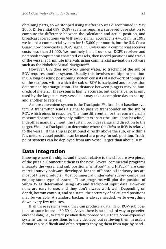
2001 Cold Water Diving for Science 85
obtaining parts, so we stopped using it after SPS was discontinued in May2000. Differential GPS (DGPS) systems require a surveyed base station tocompute the difference between the calculated and actual position, andbroadcast corrections via VHF radio signal; accuracy is +/–1-2 m. In 1995we leased a commercial system for $45,000 per month, but the U.S. CoastGuard now broadcasts a DGPS signal in Kodiak and a commercial receivercosts less than $1,000. We routinely install our own DGPS receiver andnotebook computer on chartered vessels, then record positions and tracksof the vessel at 1 minute intervals using commercial navigation softwaresuch as the Nobeltec Visual Navigator™.
However, GPS does not work under water, so tracking of the sub orROV requires another system. Usually this involves multipoint position-ing. A long-baseline positioning system consists of a network of “pingers”on the seafloor, within which the sub or ROV is navigated and its positiondetermined by triangulation. The distance between pingers may be hun-dreds of meters. This system is highly accurate, but expensive, so is onlyused by the largest survey vessels. It may take a complete day to set up,and another to retrieve.
A more convenient system is the Trackpoint™ ultra-short baseline sys-tem. A transmitter sends a signal to passive transponder on the sub orROV, which pings in response. The time differential for the return signal ismeasured between nodes only millimeters apart (the ultra-short baseline).If depth is manually input, the system provides range and direction to thetarget. We use a Trackpoint to determine where the Delta or ROV is relativeto the vessel. If the ship is positioned directly above the sub, or within afew meters, vessel position can be used as a proxy for sub position. Track-point systems can be deployed from any vessel larger than about 10 m.
Data IntegrationKnowing where the ship is, and the sub relative to the ship, are two piecesof the puzzle. Connecting them is the next. Several commercial programsintegrate the vessel and sub positions. WinFrog™ and HiPack™ are com-mercial survey software developed for the offshore oil industry (as aremost of these products). Most commercial underwater survey companiesemploy some type of system. These programs will plot the position ofSub/ROV as determined using GPS and trackpoint input data. However,none are easy to use, and they don’t always work well. Depending ondepth, bottom contour, and sea state, the accuracy of calculated positionsmay be variable. A standard backup is always needed: write everythingdown every few minutes.
If all these systems work, they can produce a data file of ROV/sub posi-tions at some interval (30-60 s). As yet there is no standard way to georefer-ence the data, i.e., to attach position data to video or CTD data. Some expensivesystems can write positions to the videotape, but retrieving them in usableformat can be difficult and often requires copying them from tape by hand.

After surveying a grid of lines with the Delta, ROV, or the BRAD-3, wereview all videotapes in the lab. Using commercial software called TheObserver™, we code all crabs seen by species, sex, maturity, activity (bur-ied, exposed, mating, feeding), and context (aggregated or not). We canalso code any other species and conditions observed. The program pro-duces a data file with each observation and a time code to the nearest 0.01second. This data file with time codes is then run through a visual basicprogram called Crabtime, which aggregates the observations by type intouser-defined intervals of 1-10 minutes, usually 2 or 5 minutes. The result-ing histogram of crabs per time interval can be plotted along with vesselpositions using a GIS program such as ArcInfo. In practice, we spend a dayon the water making 4-6 hours of sled or ROV tows. These require 1-2days to examine properly and less than an hour to integrate the data andplot it on a paper chart. The chart can then be used to guide the nextsurvey trip. If necessary, we can analyze tapes on board ship while record-ing (with the ROV) or reviewing (with the sled), create the summary file,and plot by hand on the navigation computer, in a few minutes betweensled tows. However, observations made by this method (at sea, on a pitch-ing, rolling ship) are not as accurate as those made by a rested observersitting at a stable desktop computer and video console.
Now that we have all this data, what do we do with it? According toBob Ballard, dealing with the vast amounts of information supplied byunderwater research equipment can be “like sipping water from a fire hose”(MacDonald and Juniper 1997). Indeed, it may be so difficult to catalog,store, and analyze all the data, that much of it never gets utilized or inte-grated. We store our summary crab observations (numbers per unit inter-val) and position data in a Microsoft Access™ database. Then, crab numberscan be matched up with positions for plotting, and it can even be used tocalculate offsets for the position lag between ship and sled. Most largeresearch vessels put all the data from a cruise on CD-ROMs. Then, obser-vations of organisms or habitats can be cross-referenced with depth, time,temperature, and other data, using a database. Needless to say, underwa-ter research requires a good data manager.
ConclusionsThere are many ways to conduct underwater research at depths belowsafe scuba depth. These range from inexpensive video sleds to expensivesubmersibles with lots of data integration. Selection of the best systemfor any research project always involves a compromise between cost anddata quality. Fortunately, technological improvements are occurring at sucha pace that inexpensive, high-quality systems that were unavailable fiveyears ago are now relatively affordable. We have been fortunate to cooper-ate with several labs in developing equipment that can be traded and loaned,with interchangeable parts that can be swapped as needed. Thus, the BRAD-3 sled was built by the Kodiak Lab, paid for by the Auke Bay Lab (ABL),
86 Stevens — Voyage to See What’s on the Bottom

2001 Cold Water Diving for Science 87
uses a camera housing developed by the Alaska Fisheries Science Center(AFSC), and includes camera and lighting equipment which is owned byeither the ABL, AFSC, or ADFG. As camera systems improve in the future,the sleds can be modified or built anew to accommodate them.
AcknowledgmentsMuch of our work was supported by grants from the National UnderseaResearch Program, West Coast and Polar Regions Office, University of AlaskaFairbanks. We also benefited from the assistance of Capt. Gary Edwards,FV Big Valley; and Capt. Dan Miller, FV Anna D.; David and Rich Slater, andChris Ijames of Delta Oceanographics have been very helpful. MarkBlakeslee of Aqualife Engineering has provide ROV leasing and operationfor several years. The BRAD-3 video sled was built by Jerry Chistiansen,with funds from the NMFS Auke Bay Lab. Reference to trade names in thispaper does not imply endorsement by NMFS.
ReferencesBellingham, J.G. 1997. New oceanographic uses of autonomous underwater vehi-
cles. Mar. Tech. Soc. J. 31:34-47.
MacDonald, I.R., and S.K. Juniper. 1997. Sipping from the fire-hose: How to tamethe data flow from ROV operations. Mar. Tech. Soc. J. 31:61-67.
Patterson, M.A., J.H. Sias, and D.V. Gouge. 2001. AUVs and scientific diving: A loom-ing conflict? Mar. Tech. Soc. J. 34:75-81.
Stevens, B.G., J.A. Haaga, and W.E. Donaldson. 1994. Aggregative mating of Tannercrabs Chionoecetes bairdi. Can. J. Fish. Aquat. Sci. 51:1273-1280.
Stevens, B.G., J.A. Haaga, and W.E. Donaldson. 2000a. Mound formation by Tanner crabs,Chionoecetes bairdi: Tidal phasing of larval launch pads? In: J.C.V.V. Klein and F.R.Schram (eds.), Crustacean issues 12: The biodiversity crisis and Crustacea.Proceedings of the Fourth International Crustacean Congress, Amsterdam, TheNetherlands, July 20-24, 1998. Vol. 2. A.A. Balkema, Rotterdam, pp. 445-453.
Stevens, B.G., W.E. Donaldson, J.A. Haaga, and J.E. Munk. 1993. Morphometry andmaturity of male Tanner crabs, Chionoecetes bairdi, grasping pubescent andmultiparous females in shallow and deepwater environments. Can. J. Fish.Aquat. Sci. 50:1504-1516.
Stevens, B.G., J.A. Haaga, W.E. Donaldson, and S.A. Payne. 1996. Reproductive con-ditions of prespawning multiparous female Tanner crabs (Chionoecetes bairdi)from Chiniak and Womens bays, Kodiak Island, Alaska. In: High latitude crabs:Biology, management, and economics. University of Alaska Sea Grant, AK-SG-96-02, Fairbanks. pp. 349-353.
Stevens, B.G., I. Vining, S. Byersdorfer, and W.E. Donaldson. 2000b. Ghost fishingby Tanner crab (Chionoecetes bairdi) pots off Kodiak, Alaska: Pot density andcatch per trap as determined from sidescan sonar and pot recovery data. Fish.Bull. 98:389-399.


Cold Water Diving for Science 89University of Alaska Sea Grant • AK-SG-01-06, 2001
Jellyfish Effects on Food WebProduction in the Bering SeaSteven R. WhitneyInstitute of Marine Science, University of Alaska Fairbanks,P.O. Box 757220, Fairbanks, AK 99775-7220, 907-747-5939 (tel.),907-474-5863 (fax), [email protected]
In recent years, gelatinous plankton, including large jellyfish, have beenshown to have a substantial impact upon fish populations by preying oneggs and yolk-sac larvae. In the Bering Sea, there has been a tenfold growthin the biomass of the large jellyfish Chrysaora melanaster over the pastdecade (Brodeur et al. 1999). Other than a small, one-time snapshot in latesummer (Hamner 1982), their feeding habits have not been examined andnothing is known about diets in spring; when with other species, preda-tion rates as high as 60% of the ambient fish eggs per day have beenrecorded (Purcell et al. 1994). In some systems, growth in jellyfish biom-ass has been accompanied by failure in recruitment of fish stocks. Thisstudy tests the hypothesis that Chrysaora melanaster significantly de-presses the annual production and biomass of other members of the pe-lagic food web of the Bering Sea, including walleye pollock (Theragrachalcogramma) and other forage fishes. The hypothesized mechanismsoperate through trophodynamic processes, including competition withfishes for common prey, and predation on fish eggs and larvae.
Several species of jellyfish actively select for fish eggs among theplankton (Fancett 1988, Purcell et al. 1994). When sufficient high-qualityfood is available, medusae often experience exponential growth and canquickly become the dominant species in an ecosystem. In nonintroducedspecies, this is often limited by predation from other medusae. In theBering Sea there is only one documented case of this occurring (Hamner1982), where the large jellyfish Cyanea capillata preyed upon Chrysaoramelanaster. Cyanea capillata, however, tend to be located in the outershelf and oceanic regions. Thus there may be little predation pressureupon Chrysaora in the middle and inner-shelf regions of the eastern BeringSea.
The study encompassed a two-month period from early April throughearly June 2000, the period of peak spawning of pollock on the southeast-

ern shelf as well as the suspected period of maximum growth for themedusae. It was conducted from a relatively inexpensive 9.8 m Bristol Baygillnetting vessel. The vessel size necessitated working out of a safe har-bor, such as False Pass, where shelter could be taken whenever weatherconditions were too severe for the boat or for diving. The chosen sam-pling site was the north shore of Unimak Island near the entrance to FalsePass in depths less than 20 m. This is an area of historic high jellyfishbiomass and near the center of distribution of spawning pollock. The 20m depth was chosen because it provides a floor that can be utilized forequipment as well as for safety concerns.
For the process studies, collection via diving was chosen. Due to thefragile nature of jellyfish, trawling often produces unusable specimens,since they are damaged and net contamination makes stomach contentanalysis dubious. Much of the feeding takes place on the oral lobes, whichhang below the animals and may be three meters long in Bering Sea Chrysao-ra. These are often torn off in plankton trawls. Due to the vertical compo-sition of the population (Brodeur 1998), dip-nets are also likely to collectspecimens nonrepresentative of the population and damage the oral lobesin small waves and choppy conditions. This leaves diving as an alterna-tive to collect samples.
Since there are no diving facilities in the region, a compressor wasneeded at the site. A low-pressure, surface-supply system was chosenbecause it is a small portable system weighing about 250 kg and can beplaced aboard a small vessel and run on diesel. This system also allowsfor ease of communication and cooperation with the support vessel throughthe tether. One advantage of this system is that divers are not time-limitedby tanks and are thus more able to complete tasks. The tether is neededdue to the currents, low visibility, and lack of spatial references for thedivers. This system is widely used by commercial abalone, sea cucumber,and geoduck divers in Alaska waters and is suitable for many of the re-mote diving conditions encountered here.
Although the project was designed to test different methods of collec-tion for Chrysaora melanaster via diving, the jellyfish distribution in 2000proved to be too deep, and specimens had to be collected with an ottertrawl. In future studies modifications (such as a completely ship-basedstudy and incorporation of ROV use) will need to be made in order tofollow swarms of jellyfish away from safe harbors.
ReferencesBrodeur, R.D. 1998. In situ observations of the association between juvenile fishes
and scyphomedusae in the Bering Sea. Mar. Ecol. Prog. Ser. 163:11-20.
Brodeur, R.D., C.E. Mills, J.E. Overland, G.E. Walters, and J.D. Schumacher. 1999.Evidence for a substantial increase in gelatinous zooplankton in the BeringSea, with possible links to climate change. Fish. Oceanogr. 8(4):296-306.
90 Whitney — Jellyfish Effects on Food Web Production in the Bering Sea

2001 Cold Water Diving for Science 91
Fancett, M.S. 1988. Diet and prey selectivity of scyphomedusae from Port PhillipBay, Australia. Mar. Biol. 98:503-509.
Hamner, W. 1982. Gelatinous zooplankton in the Bering Sea. Probes Final ReportVol. II.
Purcell, J.E., D.A. Nemazie, S.E. Dorsey, E.E. Houde, and J.C. Gamble. 1994. Preda-tion mortality of bay anchovy Anchoa mitchilli eggs and larvae due to scy-phomedusae and ctenophores in Chesapeake Bay. Mar. Ecol. Prog. Ser.114:47-58.


Cold Water Diving for Science 93University of Alaska Sea Grant • AK-SG-01-06, 2001
A Fisheries Habitat SurveyMethod for NearshoreEnvironments Utilizing ScubaEdward (Ted) J. Maney Jr. and Craig McMannusMarine Science Center, Northeastern University, 430 Nahant Road, EastPoint, Nahant, MA 01908, 781-581-7370 (tel.), [email protected]
Nearshore coastal environments are important fishery habitats that arehard to survey by traditional methods. Water depth is shallow and vari-able due to numerous objects and tides, making it impossible for accessby large research vessels. Using scuba, these areas can be surveyed fromshore or by small boat.
More research is required to identify and describe nearshore coastalessential fish habitats (EFH). In addition, more information is required forall life history stages complete with identification of habitat requirementsand species interactions within these environments. For most commer-cially managed species, only presence/absence data and habitat-relateddensities are known. Very little information exists for growth, reproduc-tion, or survival, as well as production rates.
We have developed a protocol utilizing the Linear Point-Intercept (LPI)Method (Ohlhorst et al. 1988, Aronson and Precht 1995), to accuratelysurvey nearshore habitats for substrate and organisms. The recreationaldiving community can utilize this relatively inexpensive and easy-to-usemethod. Hundreds of divers visit these areas every week. With propertraining, these groups can conduct surveys of nearshore coastal environ-ments. This utilization of recreational divers to conduct these surveyswould significantly increase the areas surveyed. Large amounts of fisheryhabitats could be surveyed, something which could not be done withinthe scientific or fisheries management community due to limited laborforce.
We conducted a pilot study with recreational divers to determine thefeasibility of utilizing recreational divers to conduct these surveys. Wepresent the protocol and compare results obtained using recreational diversversus scientific divers.

ReferencesAronson, R.B., and W.F. Precht. 1995. Landscape patterns of reef coral diversity: A
test of intermediate disturbance hypothesis. J. Exp. Mar. Biol. Ecol. 192:1-14.
Ohlhorst, S.L., W.D. Liddell, R.J. Taylor, and J.M. Taylor. 1988. Evaluation of reefcensus techniques. Proc. 6th Int. Coral Reef Symp., Australia, Vol. 2, pp. 319-324.
94 Maney and McMannus — A Fisheries Habitat Survey Method

Cold Water Diving for Science 95University of Alaska Sea Grant • AK-SG-01-06, 2001
Hyperpycnal Plumes in Shelf Watersof the Exuma Cays, Bahamas: ATrigger for Coral Bleaching?Patrick A. Pitts
Harbor Branch Oceanographic Institution, 5600 U.S. 1 North, Ft. Pierce,FL 34946, 561-465-2400 (tel.), 561-468-0757 (fax), [email protected]
The formation and transport of warm, high-salinity water from GreatBahama Bank to shelf waters of the Exuma Cays, Bahamas, during summermonths has been documented by a number of studies (Smith 1995, 1996;Pitts 1999). This research has shown that during summer months the ef-fects of incoming solar radiation and high evaporation on the relativelyshallow waters of Great Bahama Bank can raise the temperature and salin-ity of bank water by up to 2º C and 2 psu (practical salinity units), respec-tively, above those found in nearby Exuma Sound water. During the ebbhalf of the tidal cycle, the warm hyperpycnal bank water is forced throughtidal channels between cays onto the narrow shelf on the Exuma Soundside of the island chain. It is over this narrow shelf where most of theregion’s coral reefs are found.
Like most regions in the world where coral reefs are found, bleachingcan be a problem for corals in the Exuma Cays. First reports of bleachingin this region occurred in 1987, and since that time a number of bleachingepisodes have been reported. Some studies have suggested that when thewarm, high-salinity bank water ebbs onto the shelf it inundates nearshorereefs and causes or contributes to bleaching (Lang et al. 1988, Dennis andWicklund 1994). However, the evidence linking warm, high-salinity wateroriginating from Great Bahama Bank to bleaching of Exuma Cays reef cor-als is based mainly on inference. The physical data from these studies arelimited to comparisons of median monthly bank and shelf-water temper-atures, which obscures fluctuations over the shorter time scales. Meteoro-logically forced fluctuations, which are the most important for raisingtemperature and salinity above mean values, occur over time scales ofseveral days to about two weeks.
While studies have established the differences in characteristics be-tween bank and sound water, none have described the behavior of the

hyperpycnal bank water as it moves across and along the shelf after exit-ing through tidal inlets on the ebb tide. This paper uses hydrographicdata collected over the shelf just seaward of a tidal inlet to characterizethe top-to-bottom temperature, salinity, and density structure of hyperpy-cnal plumes after they have exited Great Bahama Bank. The objective is tocharacterize the behavior of warm, hypersaline water as it is transported bydensity currents to near-bottom shelf areas where it may trigger bleaching.
Hydrographic profiles were made at five to six equally spaced sitesalong the shelf seaward of Adderley Cut. This channel experiences vigor-ous exchanges between Great Bahama Bank and Exuma Sound, and warm,hyperpycnal bank water has been repeatedly observed moving onto theshelf through this channel. Profiles were made at or near the end of theebb tide. Water temperature, salinity, and density were recorded every 0.5seconds from the surface to the bottom at each site using a SeaBird SeaCatSBE-19 deployed from a small boat. Water depth at the sites ranged be-tween 6 and 24 m. Results from two of these hydrographic transects aredescribed below.
Measurements made on July 7, 1998, showed a very distinct warm,high-salinity plume over the shelf seaward of Adderley Cut (Figure 1). Forreference, at the time of sampling bank water in the channel had an aver-age temperature and salinity of 30.5º C and 39.8 psu, while Exuma Soundwater temperature and salinity generally averaged 29.7º C and 36.8 psu.Thus, bank water was 0.8º C warmer and 3.0 psu saltier than sound water.The top plot shows that temperatures in the plume ranged between 29.8ºC in the upper layer and 30.2ºC in the near-bottom layer. These values are0.1-0.5º C above the ambient sound temperature and 0.3-0.7º C belowbank water temperature. Thus, if the plume water sampled along thetransect was full strength bank water when it exited Adderley Cut, then bythe time the plume water reached the transect site it had entrained andmixed with sound water to the point that it was diluted between 38% (low-er layer) and 88% (upper layer). It is important to note that the weakestmixing occurred in the lowest layer so water temperatures were warmestnear the bottom where the corals are found. The bottom plot shows thatsalinity in the plume ranged between 37.5 psu in the upper layer and alittle over 39 psu near the bottom. Using salinity as a tracer, calculationssuggest a dilution of bank water by 27% near the bottom and 77% in theupper plume layer due to entrainment of sound water. A plot of waterdensity (not shown) indicates that the increase in water density due to thehigher salinity of bank water is greater than the decrease in salinity asso-ciated with warmer temperature, thus the bank water exits the channel asa hyperpycnal plume that sinks below ambient sound water.
An important feature of the plots is the lateral spreading of the plumealong the shelf in the near-bottom layers. The hyperpycnal water movedlaterally along the shelf past the northernmost and southernmost hydro-graphic stations—a distance of about 0.5 km in either direction from thecenter of the plume. The hyperpycnal water occupied most of the lower
96 Pitts — Hyperpycnal Plumes in Shelf Waters of the Exuma Cays, Bahamas

2001 Cold Water Diving for Science 97
Figure 1. Contour plots of top-to-bottom temperature (top) and salinity (bottom)profiles taken over the shelf seaward of Adderley Cut, July 7, 1998.

half of the water column as it spread to the north (toward the right on theplot), a process that was probably aided by the prevailing northward-directed along-shelf current.
Hydrographic profiles obtained on August 31, 2000, also indicated ahyperpycnal plume over the shelf (not shown), but its characteristics weredistinctly different from the plume observed on July 7. The data indicatethat lateral spreading of plume water was minimal, confining the hyper-pycnal water to a relatively narrow segment (only about 0.2 km in width)of the shelf seaward of the inlet. Within this narrow segment two regionsof hyperpycnal water were observed—one at mid-depth and one very nearthe bottom. Temperature and salinity of core plume water at these twolevels were 37.5º C and 29.8 psu, which was approximately 0.5º C warmerand 0.3 psu saltier than the surrounding Exuma Sound water. Unfortu-nately, data were not collected from Adderley Cut, so temperature andsalinity differences between bank and sound waters are unavailable forestimating mixing.
In conclusion, the hydrographic data reported here suggest that asthe hyperpycnal bank water exits the tidal passes between Exuma Cays, itsinks and can spread significant distances laterally along the shelf. Whileentrainment and mixing with Exuma Sound water is relatively strong atthe top of the plume, it is weak near the bottom and the plume movesacross and along the bottom relatively intact. Thus, it appears that warmhyperpycnal bank water can expose the benthos on the shelf to increasesin temperature and salinity above conditions to which they are normallyacclimated. This supports the hypothesis that density currents are a mech-anism for triggering coral bleaching, at least during summer months andnear the tidal inlets.
ReferencesDennis, G.D., and R.I Wicklund. 1994. The relationship between environmental fac-
tors and coral bleaching at Lee Stocking Island, Bahamas in 1990. In: R.N.Ginsburg (ed.), Global aspects of coral reefs: Health, hazards and history. Univ.of Miami, pp. 167-173.
Lang, J.C., R.I. Wicklund, and R.F. Dill. 1988. Depth- and habitat-related bleachingof zooxanthellate reef organisms near Lee Stocking Island, Exuma Cays, Baha-mas. Proceedings of the 6th International Coral Reef Symposium 3:269-274.
Pitts, P.A. 1999. Transport of warm, high-salinity water to the fringing reefs in theExuma Cays, Bahamas: Implications for coral bleaching. In: J. Heine, D. Canestro,and G. Wuttken (eds.), Proceedings of the American Academy of UnderwaterSciences 19th Annual Scientific Diving Symposium, pp. 91-101.
Smith, N.P. 1995. Observations of steady and seasonal salt, heat and mass trans-port through a tidal channel. J. Geophys. Res. 100:13,713-13,718.
Smith, N.P. 1996. The effect of hyperpycnal water on tidal exchanges. In: D.G. Aubreyand C.T. Friedrichs (eds.), Buoyancy effects of coastal and estuarine dynamics.Coastal and Estuarine Studies 53:107-116.
98 Pitts — Hyperpycnal Plumes in Shelf Waters of the Exuma Cays, Bahamas