coinductive foundations of infinitary ...coinductive foundations of infinitary rewriting and...
TRANSCRIPT

Logical Methods in Computer ScienceVol. 14(1:3)2018, pp. 1–44www.lmcs-online.org
Submitted Jun. 1, 2016Published Jan. 10, 2018
COINDUCTIVE FOUNDATIONS
OF INFINITARY REWRITING
AND INFINITARY EQUATIONAL LOGIC ∗
JORG ENDRULLIS a, HELLE HVID HANSEN b, DIMITRI HENDRIKS c, ANDREW POLONSKY d,AND ALEXANDRA SILVA e
a,c Department of Computer Science, VU University Amsterdam, The Netherlandse-mail address: {j.endrullis, r.d.a.hendriks}@vu.nl
b Department of Engineering Systems and Services, Delft University of Technology, The Netherlandse-mail address: [email protected]
d Institut de Recherche en Informatique Fondamentale, Paris Diderot University, Francee-mail address: [email protected]
e Department of Computer Science, University College London, Englande-mail address: [email protected]
Abstract. We present a coinductive framework for defining and reasoning about the
infinitary analogues of equational logic and term rewriting in a uniform way. We define∞=,
the infinitary extension of a given equational theory =R, and →∞, the standard notion ofinfinitary rewriting associated to a reduction relation →R, as follows:
∞= := νR. (=R ∪ R)∗
→∞ := µR. νS. (→R ∪ R)∗ ; S
Here µ and ν are the least and greatest fixed-point operators, respectively, and
R := { 〈f(s1, . . . , sn), f(t1, . . . , tn)〉 | f ∈ Σ, s1R t1, . . . , snR tn } ∪ Id .
The setup captures rewrite sequences of arbitrary ordinal length, but it has neither theneed for ordinals nor for metric convergence. This makes the framework especially suitablefor formalizations in theorem provers.
1. Introduction
We present a coinductive framework for defining infinitary equational reasoning and infinitaryrewriting in a uniform way. The framework is free of ordinals, metric convergence and partialorders on terms which have been essential in earlier definitions of the concept of infinitaryrewriting [12, 28, 31, 27, 26, 3, 2, 4, 21].
Infinitary rewriting is a generalization of the ordinary finitary rewriting to infinite termsand infinite reductions (including reductions of ordinal length greater than ω). For the
Key words and phrases: infinitary rewriting, infinitary equational reasoning, coinduction.∗ This is a modified and extended version of [16] which appeared in the proceedings of RTA 2015.
LOGICAL METHODSl IN COMPUTER SCIENCE DOI:10.23638/LMCS-14(1:3)2018c© J. Endrullis, H. N. Hansen, D. Hendriks, A. Polonsky, and A. SilvaCC© Creative Commons

2 J. ENDRULLIS, H. N. HANSEN, D. HENDRIKS, A. POLONSKY, AND A. SILVA
definition of rewrite sequences of ordinal length, there is a design choice concerning theexclusion of jumps at limit ordinals, as illustrated in the ill-formed rewrite sequence
a→ a→ a→ · · ·︸ ︷︷ ︸ω-many steps
b→ b
where the rewrite system is R = { a→ a, b→ b }. The rewrite sequence remains for ω stepsat a and in the limit step ‘jumps’ to b. To ensure connectedness at limit ordinals, the usualchoices are:
(i) weak convergence (also called ‘Cauchy convergence’), where it suffices that the sequenceof terms converges towards the limit term, and
(ii) strong convergence, which additionally requires that the ‘rewriting activity’, i.e., thedepth of the rewrite steps, tends to infinity when approaching the limit.
The notion of strong convergence incorporates the flavor of ‘progress’, or ‘productivity’, inthe sense that there is only a finite number of rewrite steps at every depth. Moreover, itleads to a more satisfactory metatheory where redex occurrences can be traced over limitsteps.
While infinitary rewriting has been studied extensively, notions of infinitary equationalreasoning have not received much attention. Some of the few works in this area are byKahrs [26] and by Lombardi, Rıos and de Vrijer [32], see Related Work below. The reasonis that the usual definition of infinitary rewriting is based on ordinals to index the rewritesteps, and hence the rewrite direction is incorporated from the start. This is different for theframework we propose here, which enables us to define several natural notions: infinitaryequational reasoning, bi-infinite rewriting, and the standard concept of infinitary rewriting.All of these have strong convergence ‘built-in’.
We define infinitary equational reasoning with respect to a system of equations R, as a
relation∞= on potentially infinite terms by the following mutually coinductive rules:
s (=R ∪∞↽⇁)∗ t
s∞= t
s1∞= t1 · · · sn
∞= tn
f(s1, s2, . . . , sn)∞↽⇁ f(t1, t2, . . . , tn)
(1.1)
The relation∞↽⇁ stands for infinitary equational reasoning below the root. The coinductive
nature of the rules means that the proof trees need not be well-founded. Reading the rulesbottom-up, the first rule allows for an arbitrary, but finite, number of rewrite steps at anyfinite depth (of the term tree). The second rule enforces that we eventually proceed withthe arguments, and hence the activity tends to infinity.
Cω∞= a
Cω∞↽⇁ C(a) C(a) =R a
Cω∞= a
Figure 1: Derivation of Cω∞= a.
COINDUCTIVE FOUNDATIONS OF INFINITARY REWRITING AND EQUATIONAL LOGIC 3
Example 1.1. Let R consist of the equation
C(a) = a .
We write Cω to denote the infinite term C(C(C(. . .))), the solution of the equation X = C(X).
Using the rules (1.1), we can derive Cω∞= a as shown in Figure 1. This is an infinite proof
tree as indicated by the loop in which the sequence Cω∞↽⇁ C(a) =R a is written by
juxtaposing Cω∞↽⇁ C(a) and C(a) =R a.
Many of the proof trees we consider in this paper are regular trees, that is, trees havingonly a finite number of distinct subtrees. These infinite trees are convenient since theycan be depicted by a ‘finite tree’ enriched with loops . However, we emphasise that ourframework is not limited to regular trees.
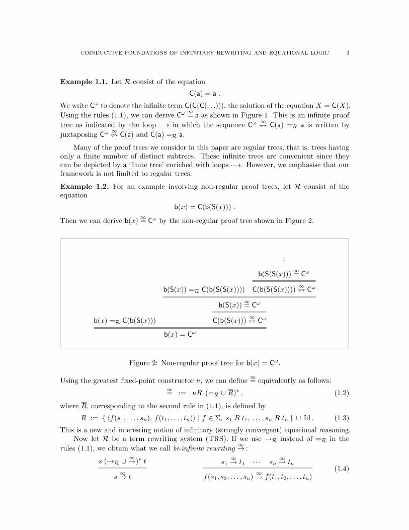
Example 1.2. For an example involving non-regular proof trees, let R consist of theequation
b(x) = C(b(S(x))) .
Then we can derive b(x)∞= Cω by the non-regular proof tree shown in Figure 2.
b(x) =R C(b(S(x)))
b(S(x)) =R C(b(S(S(x))))
...
b(S(S(x)))∞= Cω
C(b(S(S(x))))∞↽⇁ Cω
b(S(x))∞= Cω
C(b(S(x)))∞↽⇁ Cω
b(x) = Cω
Figure 2: Non-regular proof tree for b(x) = Cω.
Using the greatest fixed-point constructor ν, we can define∞= equivalently as follows:
∞= := νR. (=R ∪ R)∗ , (1.2)
where R, corresponding to the second rule in (1.1), is defined by
R := { 〈f(s1, . . . , sn), f(t1, . . . , tn)〉 | f ∈ Σ, s1 R t1, . . . , sn R tn } ∪ Id . (1.3)
This is a new and interesting notion of infinitary (strongly convergent) equational reasoning.Now let R be a term rewriting system (TRS). If we use →R instead of =R in the
rules (1.1), we obtain what we call bi-infinite rewriting∞→ :
s (→R ∪∞⇁)∗ t
s∞→ t
s1∞→ t1 · · · sn
∞→ tn
f(s1, s2, . . . , sn)∞⇁ f(t1, t2, . . . , tn)
(1.4)
4 J. ENDRULLIS, H. N. HANSEN, D. HENDRIKS, A. POLONSKY, AND A. SILVA
corresponding to the following fixed-point definition:∞→ := νR. (→R ∪ R)∗ . (1.5)
We write∞→ to distinguish bi-infinite rewriting from the standard notion →∞ of (strongly
convergent) infinitary rewriting [35]. The symbol ∞ is centered above → in∞→ to indicate
that bi-infinite rewriting is ‘balanced’, in the sense that it allows rewrite sequences to beextended infinitely forwards, but also infinitely backwards. Here backwards does not refer toreversing the arrow ←R. For example, for R = {C(a)→ a } we have the backward-infinite
rewrite sequence · · · → C(C(a))→ C(a)→ a and hence Cω∞→ a. The proof tree for Cω
∞→ a
has the same shape as the proof tree displayed in Figure 1; the only difference is that∞= is
replaced by∞→ and
∞↽⇁ by
∞⇁. In contrast, the standard notion →∞ of infinitary rewriting
only takes into account forward limits and we do not have Cω →∞ a.We have the following strict inclusions:
→∞ ( ∞→ ( ∞= (1.6)
In our framework, these inclusions follow directly from the fact that the proof trees for →∞(see below) are a restriction of the proof trees for
∞→ which in turn are a restriction of the
proof trees for∞=. It is also easy to see that each inclusion is strict. For the first, see above.
For the second, just note that∞→ is not symmetric.
Finally, by a further restriction of the proof trees, we obtain the standard concept of(strongly convergent) infinitary rewriting→∞. Using least and greatest fixed-point operators,we define:
→∞ := µR. νS. (→ ∪ R)∗ ; S , (1.7)
where ; denotes relational composition in diagrammatic order, that is:
x (R ; S) y ⇐⇒ ∃z. x R z ∧ z S y .The greatest fixed point defined using the variable S is a coinductively defined relation.Thus only the last step in the sequence (→ ∪ R)∗ ; S is coinductive. This corresponds to thefollowing fact about reductions σ of ordinal length: every strict prefix of σ must be shorterthan σ itself, while strict suffixes may have the same length as σ.
If we replace µ by ν in (1.7), we get a definition equivalent to∞→ defined by (1.5). To
see that it is at least as strong, note that Id ⊆ S.Conversely, →∞ can be obtained by a restriction of the proof trees obtained by the
rules (1.4) for∞→. Assume that in a proof tree using the rules (1.4), we mark those occurrences
of∞⇁ that are followed by another step in the premise of the rule (i.e., those that are not
the last step in the premise). Thus we split∞⇁ into ⇁∞ and
<⇁∞. Then the restriction to
obtain the relation →∞ is to forbid infinite nesting of marked symbols<⇁∞. This marking
is made precise in the following rules:
s (→ ∪ <⇁∞)∗ ; ⇁∞ t
s→∞ t
s1 →∞ t1 · · · sn →∞ tn
f(s1, s2, . . . , sn) (<)⇁∞ f(t1, t2, . . . , tn) s (<)⇁∞ s(1.8)
Here ⇁∞ stands for infinitary rewriting below the root, and<⇁∞ is its marked version.
The symbol (<)⇁∞ stands for both ⇁∞ and<⇁∞. Correspondingly, the rule in the middle is
an abbreviation for two rules. The axiom s ⇁∞ s serves to ‘restore’ reflexivity, that is, it
COINDUCTIVE FOUNDATIONS OF INFINITARY REWRITING AND EQUATIONAL LOGIC 5
models the identity steps in S in (1.7). Intuitively, s<⇁∞ t can be thought of as an infinitary
rewrite sequence below the root, shorter than the sequence we are defining.We have an infinitary strongly convergent rewrite sequence from s to t if and only if
s →∞ t can be derived by the rules (1.8) in a (not necessarily well-founded) proof treewithout infinite nesting of
<⇁∞, that is, proof trees in which all paths (ascending through
the proof tree) contain only finitely many occurrences of<⇁∞. The depth requirement in the
definition of strong convergence arises naturally in the rules (1.8), in particular the middlerule pushes the activity to the arguments.
The fact that the rules (1.8) capture the infinitary rewriting relation→∞ is a consequenceof a result due to [28] which states that every strongly convergent rewrite sequence containsonly a finite number of steps at any depth d ∈ N, in particular only a finite number of rootsteps →ε. Hence every strongly convergent reduction is of the form (
<⇁∞ ;→ε)
∗; ⇁∞ as inthe premise of the first rule, where the steps
<⇁∞ are reductions of shorter length.
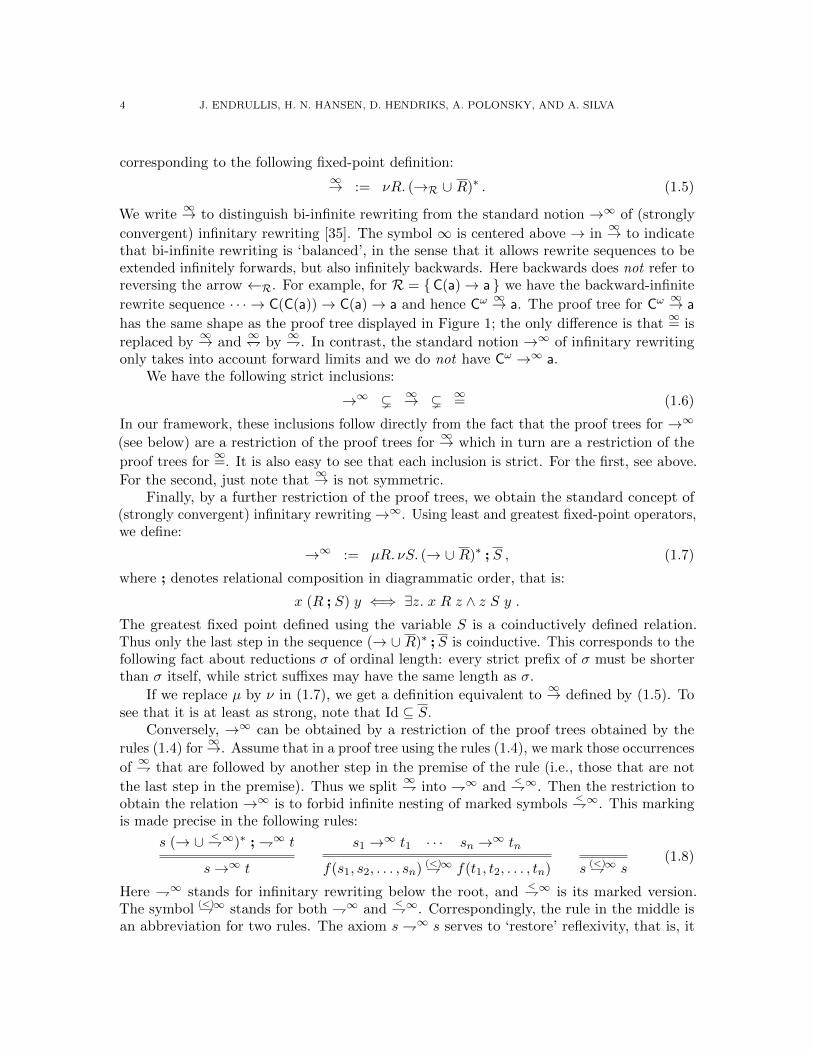
We conclude with an example of a TRS that allows for a rewrite sequence of lengthbeyond ω.
a→ε C(a)
a→∞ Cω
C(a) ⇁∞ Cω
a→∞ Cω
Figure 3: A reduction a→∞ Cω.
like Figure 3
a→∞ Cω
like Figure 3
b→∞ Cω
f(a, b)<⇁∞ f(Cω,Cω) f(Cω,Cω)→ε D
f(a, b)→∞ D
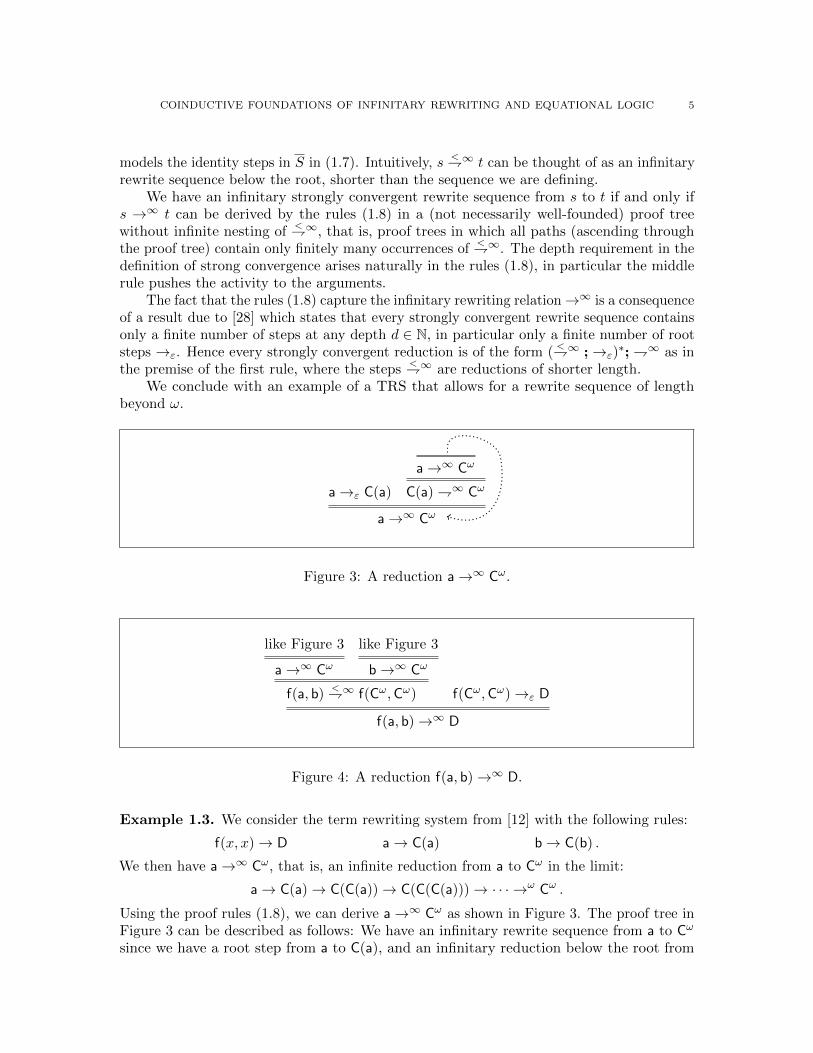
Figure 4: A reduction f(a, b)→∞ D.
Example 1.3. We consider the term rewriting system from [12] with the following rules:
f(x, x)→ D a→ C(a) b→ C(b) .
We then have a→∞ Cω, that is, an infinite reduction from a to Cω in the limit:
a→ C(a)→ C(C(a))→ C(C(C(a)))→ · · · →ω Cω .
Using the proof rules (1.8), we can derive a→∞ Cω as shown in Figure 3. The proof tree inFigure 3 can be described as follows: We have an infinitary rewrite sequence from a to Cω
since we have a root step from a to C(a), and an infinitary reduction below the root from

6 J. ENDRULLIS, H. N. HANSEN, D. HENDRIKS, A. POLONSKY, AND A. SILVA
C(a) to Cω. The latter reduction C(a) ⇁∞ Cω is in turn witnessed by the infinitary rewritesequence a→∞ Cω on the direct subterms.
We also have the following reduction, now of length ω + 1:
f(a, b)→ f(C(a), b)→ f(C(a),C(b))→ · · · →ω f(Cω,Cω)→ D .
That is, after an infinite rewrite sequence of length ω, we reach the limit term f(Cω,Cω), andwe then continue with a rewrite step from f(Cω,Cω) to D. Figure 4 shows how this rewritesequence f(a, b)→∞ D can be derived in our setup. We note that the rewrite sequencef(a, b)→∞ D cannot be ‘compressed’ to length ω. So there is no reduction f(a, b)→≤ω D.
Related Work. While a coinductive treatment of infinitary rewriting is not new [8, 25, 22],the previous approaches only capture rewrite sequences of length at most ω. The coinductiveframework that we present here captures all strongly convergent rewrite sequences of arbitraryordinal length.
From the topological perspective, various notions of infinitary rewriting and infinitaryequational reasoning have been studied in [26]. The closure operator SE from [26] is closely
related to our notion of infinitary equational reasoning∞=. The operator SE is defined by
SE(R) = (S ◦ E)?(R) where
(i) E(R) is the equivalence closure of R, and(ii) S(R) is the strongly convergent rewrite relation obtained from (single steps) R,(iii) and f?(R) is defined as µx.R ∪ f(x).
Although defined in very different ways, the relations SE(→) and∞= typically coincide.
In [32], Lombardi, Rıos and de Vrijer introduce infinitary equational reasoning based onlimits to reason about permutation equivalence of infinitary reductions that are modelled byproof terms.
Martijn Vermaat has formalized infinitary rewriting using metric convergence (in placeof strong convergence) in the Coq proof assistant [36], and proved that weakly orthogonalinfinitary rewriting does not have the property UN of unique normal forms, see [20]. Whilehis formalization could be extended to strong convergence, it remains to be investigated towhat extent it can be used for the further development of the theory of infinitary rewriting.
Ketema and Simonsen [29] introduce the notion of ‘computable infinite reductions’ [29],where terms as well as reductions are computable, and provide a Haskell implementation ofthe Compression Lemma for this notion of reduction.
This current paper is an extended version of [16]. The most important changes are:
(i) We have introduced a novel notion of permutation equivalence on infinitary rewritesequences, which we call parallel permutation equivalence. We show that two rewritesequences are parallel permutation equivalent if and only if they are represented bythe same proof tree in our framework, see Section 8.
(ii) We have rewritten and extended the description of the Coq formalisation of theCompression Lemma (Section 9).

COINDUCTIVE FOUNDATIONS OF INFINITARY REWRITING AND EQUATIONAL LOGIC 7
Outline. In Section 2 we introduce infinitary rewriting in the usual way based on ordinals,and with convergence at every limit ordinal. Section 3 is a short explanation of (co)inductionand fixed-point rules. The two new definitions of infinitary rewriting →∞ based on mixinginduction and coinduction, as well as their equivalence, are spelled out in Section 4. Then,in Section 5, we prove the equivalence of these new definitions of infinitary rewriting with
the standard definition. In Section 6 we present the above introduced relations∞= and
∞→ ofinfinitary equational reasoning and bi-infinite rewriting. In Section 7 we compare the three
relations∞=,∞→ and →∞. In Section 8 we present our new work on parallel permutation
equivalence and canonical proof trees. As an application, we show in Section 9 that ourframework is suitable for formalizations in theorem provers. We conclude in Section 10.
2. Preliminaries on Term Rewriting
We give a brief introduction to infinitary rewriting. For further reading on infinitary rewritingwe refer to [31, 35, 6, 21], for an introduction to finitary rewriting to [30, 35, 1, 5].
A signature Σ is a set of symbols f each having a fixed arity ar(f) ∈ N. Let X be aninfinite set of variables such that X ∩ Σ = ∅. The set Ter∞(Σ,X ) of (finite and) infiniteterms over Σ and X is coinductively defined by the following grammar:
t ::=co x | f( t, . . . , t︸ ︷︷ ︸ar(f) times
) (x ∈ X , f ∈ Σ) .
This means that Ter∞(Σ,X ) is defined as the largest set T such that for all t ∈ T , eithert ∈ X or t = f(t1, t2, . . . , tn) for some f ∈ Σ with ar(f) = n and t1, t2, . . . , tn ∈ T . So thegrammar rules may be applied an infinite number of times, and equality on the terms isbisimilarity. See further Section 3 for a brief introduction to coinduction.
We write Id for the identity relation on terms, Id := {〈s, s〉 | s ∈ Ter∞(Σ,X )}.
Remark 2.1. Alternatively, the set Ter∞(Σ,X ) arises from the set of finite terms, Ter(Σ,X ),by metric completion, using the well-known distance function d defined by d(t, s) = 2−n ifthe n-th level of the terms t, s ∈ Ter(Σ,X ) (viewed as labeled trees) is the first level wherea difference appears, in case t and s are not identical; furthermore, d(t, t) = 0. It is standardthat this construction yields 〈Ter(Σ,X ), d〉 as a metric space. Now, infinite terms areobtained by taking the completion of this metric space, and they are represented by infinitetrees. We will refer to the complete metric space arising in this way as 〈Ter∞(Σ,X ), d〉,where Ter∞(Σ,X ) is the set of finite and infinite terms over Σ.
Let t ∈ Ter∞(Σ,X ) be a finite or infinite term. The set of positions Pos(t) ⊆ N∗ of tis defined by: ε ∈ Pos(t), and ip ∈ Pos(t) whenever t = f(t1, . . . , tn) with 1 ≤ i ≤ n andp ∈ Pos(ti). For p ∈ Pos(t), the subterm t|p of t at position p is defined by t|ε = t andf(t1, . . . , tn)|ip = ti|p. The set of variables Var(t) ⊆ X of t is Var(t) = {x ∈ X | ∃ p ∈Pos(t). t|p = x}.
A substitution σ is a map σ : X → Ter∞(Σ,X ); its domain is extended to Ter∞(Σ,X )essentially by corecursion: σ(f(t1, . . . , tn)) = f(σ(t1), . . . , σ(tn)) (cf. [33, Example 2.5(iv)and Remark 3.2]). For a term t and a substitution σ, we write tσ for σ(t). We write x 7→ sfor the substitution defined by σ(x) = s and σ(y) = y for all y 6= x. Let � be a fresh variable.A context C is a term Ter∞(Σ,X ∪ {�}) containing precisely one occurrence of �. Forcontexts C and terms s we write C[s] for C(� 7→ s).
8 J. ENDRULLIS, H. N. HANSEN, D. HENDRIKS, A. POLONSKY, AND A. SILVA
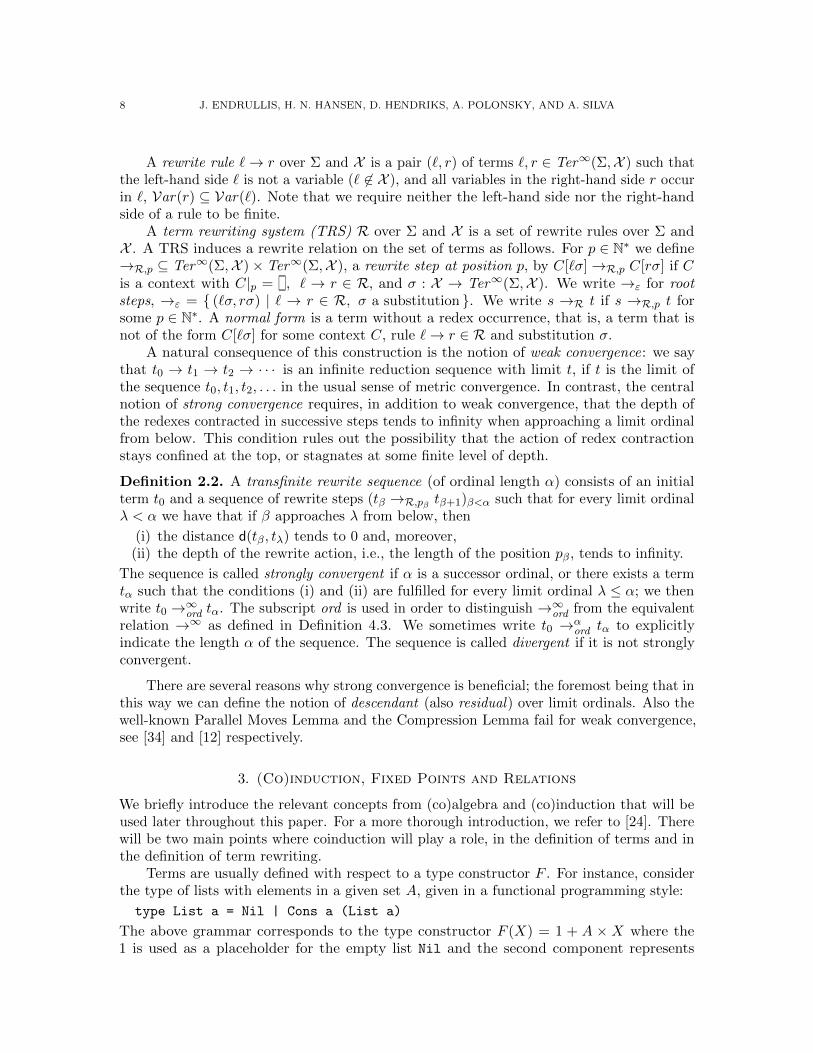
A rewrite rule `→ r over Σ and X is a pair (`, r) of terms `, r ∈ Ter∞(Σ,X ) such thatthe left-hand side ` is not a variable (` 6∈ X ), and all variables in the right-hand side r occurin `, Var(r) ⊆ Var(`). Note that we require neither the left-hand side nor the right-handside of a rule to be finite.
A term rewriting system (TRS) R over Σ and X is a set of rewrite rules over Σ andX . A TRS induces a rewrite relation on the set of terms as follows. For p ∈ N∗ we define→R,p ⊆ Ter∞(Σ,X )× Ter∞(Σ,X ), a rewrite step at position p, by C[`σ]→R,p C[rσ] if Cis a context with C|p = �, ` → r ∈ R, and σ : X → Ter∞(Σ,X ). We write →ε for rootsteps, →ε = { (`σ, rσ) | ` → r ∈ R, σ a substitution }. We write s →R t if s →R,p t forsome p ∈ N∗. A normal form is a term without a redex occurrence, that is, a term that isnot of the form C[`σ] for some context C, rule `→ r ∈ R and substitution σ.
A natural consequence of this construction is the notion of weak convergence: we saythat t0 → t1 → t2 → · · · is an infinite reduction sequence with limit t, if t is the limit ofthe sequence t0, t1, t2, . . . in the usual sense of metric convergence. In contrast, the centralnotion of strong convergence requires, in addition to weak convergence, that the depth ofthe redexes contracted in successive steps tends to infinity when approaching a limit ordinalfrom below. This condition rules out the possibility that the action of redex contractionstays confined at the top, or stagnates at some finite level of depth.
Definition 2.2. A transfinite rewrite sequence (of ordinal length α) consists of an initialterm t0 and a sequence of rewrite steps (tβ →R,pβ tβ+1)β<α such that for every limit ordinalλ < α we have that if β approaches λ from below, then
(i) the distance d(tβ, tλ) tends to 0 and, moreover,(ii) the depth of the rewrite action, i.e., the length of the position pβ, tends to infinity.
The sequence is called strongly convergent if α is a successor ordinal, or there exists a termtα such that the conditions (i) and (ii) are fulfilled for every limit ordinal λ ≤ α; we thenwrite t0 →∞ord tα. The subscript ord is used in order to distinguish →∞ord from the equivalentrelation →∞ as defined in Definition 4.3. We sometimes write t0 →α
ord tα to explicitlyindicate the length α of the sequence. The sequence is called divergent if it is not stronglyconvergent.
There are several reasons why strong convergence is beneficial; the foremost being that inthis way we can define the notion of descendant (also residual) over limit ordinals. Also thewell-known Parallel Moves Lemma and the Compression Lemma fail for weak convergence,see [34] and [12] respectively.
3. (Co)induction, Fixed Points and Relations
We briefly introduce the relevant concepts from (co)algebra and (co)induction that will beused later throughout this paper. For a more thorough introduction, we refer to [24]. Therewill be two main points where coinduction will play a role, in the definition of terms and inthe definition of term rewriting.
Terms are usually defined with respect to a type constructor F . For instance, considerthe type of lists with elements in a given set A, given in a functional programming style:
type List a = Nil | Cons a (List a)
The above grammar corresponds to the type constructor F (X) = 1 + A × X where the1 is used as a placeholder for the empty list Nil and the second component represents
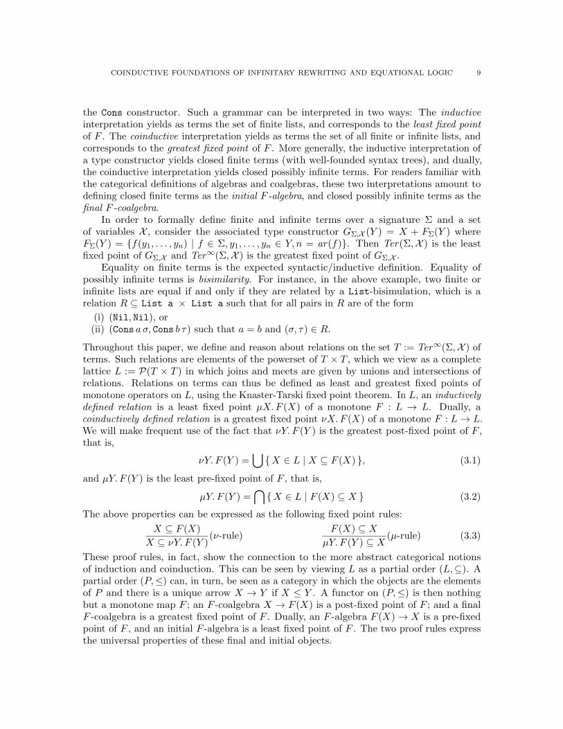
COINDUCTIVE FOUNDATIONS OF INFINITARY REWRITING AND EQUATIONAL LOGIC 9
the Cons constructor. Such a grammar can be interpreted in two ways: The inductiveinterpretation yields as terms the set of finite lists, and corresponds to the least fixed pointof F . The coinductive interpretation yields as terms the set of all finite or infinite lists, andcorresponds to the greatest fixed point of F . More generally, the inductive interpretation ofa type constructor yields closed finite terms (with well-founded syntax trees), and dually,the coinductive interpretation yields closed possibly infinite terms. For readers familiar withthe categorical definitions of algebras and coalgebras, these two interpretations amount todefining closed finite terms as the initial F -algebra, and closed possibly infinite terms as thefinal F -coalgebra.
In order to formally define finite and infinite terms over a signature Σ and a setof variables X , consider the associated type constructor GΣ,X (Y ) = X + FΣ(Y ) whereFΣ(Y ) = {f(y1, . . . , yn) | f ∈ Σ, y1, . . . , yn ∈ Y, n = ar(f)}. Then Ter(Σ,X ) is the leastfixed point of GΣ,X and Ter∞(Σ,X ) is the greatest fixed point of GΣ,X .
Equality on finite terms is the expected syntactic/inductive definition. Equality ofpossibly infinite terms is bisimilarity. For instance, in the above example, two finite orinfinite lists are equal if and only if they are related by a List-bisimulation, which is arelation R ⊆ List a × List a such that for all pairs in R are of the form
(i) (Nil, Nil), or(ii) (Cons a σ, Cons b τ) such that a = b and (σ, τ) ∈ R.
Throughout this paper, we define and reason about relations on the set T := Ter∞(Σ,X ) ofterms. Such relations are elements of the powerset of T × T , which we view as a completelattice L := P(T × T ) in which joins and meets are given by unions and intersections ofrelations. Relations on terms can thus be defined as least and greatest fixed points ofmonotone operators on L, using the Knaster-Tarski fixed point theorem. In L, an inductivelydefined relation is a least fixed point µX.F (X) of a monotone F : L → L. Dually, acoinductively defined relation is a greatest fixed point νX.F (X) of a monotone F : L→ L.We will make frequent use of the fact that νY. F (Y ) is the greatest post-fixed point of F ,that is,
νY. F (Y ) =⋃{X ∈ L | X ⊆ F (X) }, (3.1)
and µY. F (Y ) is the least pre-fixed point of F , that is,
µY. F (Y ) =⋂{X ∈ L | F (X) ⊆ X } (3.2)
The above properties can be expressed as the following fixed point rules:
X ⊆ F (X)
X ⊆ νY. F (Y )(ν-rule)
F (X) ⊆ XµY. F (Y ) ⊆ X
(µ-rule) (3.3)
These proof rules, in fact, show the connection to the more abstract categorical notionsof induction and coinduction. This can be seen by viewing L as a partial order (L,⊆). Apartial order (P,≤) can, in turn, be seen as a category in which the objects are the elementsof P and there is a unique arrow X → Y if X ≤ Y . A functor on (P,≤) is then nothingbut a monotone map F ; an F -coalgebra X → F (X) is a post-fixed point of F ; and a finalF -coalgebra is a greatest fixed point of F . Dually, an F -algebra F (X)→ X is a pre-fixedpoint of F , and an initial F -algebra is a least fixed point of F . The two proof rules expressthe universal properties of these final and initial objects.

10 J. ENDRULLIS, H. N. HANSEN, D. HENDRIKS, A. POLONSKY, AND A. SILVA
We will use a number of basic operations on relations. These include union (∪), reflexive,transitive closure (∗), relation composition in diagrammatic order (;), and relation liftingwhich we define now.
Definition 3.1. For a relation R ⊆ T × T we define its lifting R (with respect to Σ) by
R := { 〈f(s1, . . . , sn), f(t1, . . . , tn)〉 | f ∈ Σ, ar(f) = n , s1 R t1, . . . , sn R tn } ∪ Id .
It is straightforward to verify that all these operations are monotone (in all arguments).Hence any map F : L→ L built from these operations will have a unique least and greatestfixed point.
4. New Definitions of Infinitary Term Rewriting
We present two new definitions of infinitary rewriting s→∞ t, based on mixing inductionand coinduction, and prove their equivalence. In Section 5 we show they are equivalent tothe standard definition based on ordinals. We summarize the definitions:
A. Derivation Rules. First, we define s→∞ t via a syntactic restriction on the proof treesthat arise from the coinductive rules (1.8). The restriction excludes all proof trees thatcontain ascending paths with an infinite number of marked symbols.
B. Mixed Induction and Coinduction. Second, we define s→∞ t based on mutually mixinginduction and coinduction, that is, least fixed points µ and greatest fixed points ν.
In contrast to previous coinductive definitions [8, 25, 22], the setup proposed here capturesall strongly convergent rewrite sequences (of arbitrary ordinal length).
Throughout this section, we fix a signature Σ and a term rewriting system R over Σ.We also abbreviate T := Ter∞(Σ,X ).
Notation 4.1. Instead of introducing separate derivation rules for transitivity, we write areduction of the form s0 s1 · · · sn as a sequence of single steps:
s0 s1 s1 s2 · · · sn−1 sn
conclusion
This allows us to write the subproof immediately above a single step.
4.1. Derivation Rules.
Definition 4.2. We define the relation →∞ ⊂ T × T as follows. We have s→∞ t if thereexists a (finite or infinite) proof tree δ deriving s→∞ t using the following five rules:
s (<⇁∞ ∪ →ε)
∗ ; ⇁∞ t
s→∞ tsplit
s1 →∞ t1 · · · sn →∞ tn
f(s1, s2, . . . , sn) (<)⇁∞ f(t1, t2, . . . , tn)lift
s (<)⇁∞ sid
such that δ does not contain an infinite nesting of<⇁∞, that is, such that there exists no
path ascending through the proof tree that meets an infinite number of symbols<⇁∞. The
symbol (<)⇁∞ stands for ⇁∞ or<⇁∞; so the second rule is an abbreviation for two rules;
similarly for the third rule.
COINDUCTIVE FOUNDATIONS OF INFINITARY REWRITING AND EQUATIONAL LOGIC 11
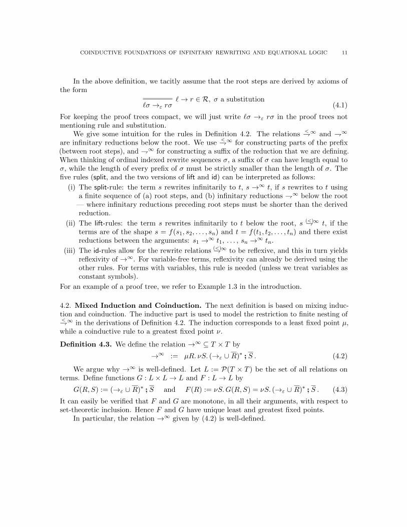
In the above definition, we tacitly assume that the root steps are derived by axioms ofthe form
`σ →ε rσ`→ r ∈ R, σ a substitution
(4.1)
For keeping the proof trees compact, we will just write `σ →ε rσ in the proof trees notmentioning rule and substitution.
We give some intuition for the rules in Definition 4.2. The relations<⇁∞ and ⇁∞
are infinitary reductions below the root. We use<⇁∞ for constructing parts of the prefix
(between root steps), and ⇁∞ for constructing a suffix of the reduction that we are defining.When thinking of ordinal indexed rewrite sequences σ, a suffix of σ can have length equal toσ, while the length of every prefix of σ must be strictly smaller than the length of σ. Thefive rules (split, and the two versions of lift and id) can be interpreted as follows:
(i) The split-rule: the term s rewrites infinitarily to t, s →∞ t, if s rewrites to t usinga finite sequence of (a) root steps, and (b) infinitary reductions ⇁∞ below the root
— where infinitary reductions preceding root steps must be shorter than the derivedreduction.
(ii) The lift-rules: the term s rewrites infinitarily to t below the root, s (<)⇁∞ t, if theterms are of the shape s = f(s1, s2, . . . , sn) and t = f(t1, t2, . . . , tn) and there existreductions between the arguments: s1 →∞ t1, . . . , sn →∞ tn.
(iii) The id-rules allow for the rewrite relations (<)⇁∞ to be reflexive, and this in turn yieldsreflexivity of →∞. For variable-free terms, reflexivity can already be derived using theother rules. For terms with variables, this rule is needed (unless we treat variables asconstant symbols).
For an example of a proof tree, we refer to Example 1.3 in the introduction.
4.2. Mixed Induction and Coinduction. The next definition is based on mixing induc-tion and coinduction. The inductive part is used to model the restriction to finite nesting of<⇁∞ in the derivations of Definition 4.2. The induction corresponds to a least fixed point µ,while a coinductive rule to a greatest fixed point ν.
Definition 4.3. We define the relation →∞ ⊆ T × T by
→∞ := µR. νS. (→ε ∪ R)∗ ; S . (4.2)
We argue why →∞ is well-defined. Let L := P(T × T ) be the set of all relations onterms. Define functions G : L× L→ L and F : L→ L by
G(R,S) := (→ε ∪ R)∗ ; S and F (R) := νS.G(R,S) = νS. (→ε ∪ R)∗ ; S . (4.3)
It can easily be verified that F and G are monotone, in all their arguments, with respect toset-theoretic inclusion. Hence F and G have unique least and greatest fixed points.
In particular, the relation →∞ given by (4.2) is well-defined.
12 J. ENDRULLIS, H. N. HANSEN, D. HENDRIKS, A. POLONSKY, AND A. SILVA
4.3. Equivalence. We show equivalence of Definitions 4.2 and 4.3. Intuitively, the µRin the fixed point definition corresponds to the nesting restriction in the definition usingderivation rules. If one thinks of Definition 4.3 as µR.F (R) with F (R) = νS.G(R,S) (seeequation (4.3)), then Fn+1(∅) are all infinite rewrite sequences that can be derived usingproof trees where the nesting depth of the marked symbol
<⇁∞ is at most n.
To avoid confusion we write →∞der for the relation →∞ defined in Definition 4.2, and→∞fp for the relation →∞ defined in Definition 4.3. We show →∞der = →∞fp . Definition 4.2requires that the nesting structure of
<⇁∞der in proof trees is well-founded. As a consequence,
we can associate to every proof tree a (countable) ordinal that allows to embed the nestingstructure in an order-preserving way. We use ω1 to denote the first uncountable ordinal, andwe view ordinals as the set of all smaller ordinals (then the elements of ω1 are all countableordinals).
Definition 4.4. Let δ be a proof tree as in Definition 4.2, and let α be an ordinal. Anα-labeling of δ is a labeling of all symbols
<⇁∞der in δ with elements from α such that each
label is strictly greater than all labels occurring in the subtrees (all labels above).
Lemma 4.5. Every proof tree as in Definition 4.2 has an α-labeling for some α ∈ ω1.
Proof. Let δ be a proof tree and let L(δ) be the set of positions of the symbol<⇁∞der in δ.
For positions p, q ∈ L(δ) we write p < q if p is a strict prefix of q. Then we have that <−1 iswell-founded, that is, there is no infinite sequence p0 < p1 < p2 < · · · with pi ∈ L(δ) (i ≥ 0)as a consequence of the nesting restriction on
<⇁∞der.
By transfinite recursion, the well-founded order on L(δ) extends to a well-order, isomor-phic to some ordinal α — and α < ω1 since L(δ) is a countable set.
Definition 4.6. Let δ be a proof tree as in Definition 4.2. We define the nesting depth of δas the least ordinal α ∈ ω1 such that δ admits an α-labeling. For every α ≤ ω1, we definea relation →∞α,der ⊆ →∞der as follows: s →∞α,der t whenever s →∞der t can be derived using aproof with nesting depth < α. Likewise we define relations ⇁∞α,der and
<⇁∞α,der .
As a direct consequence of Lemma 4.5 we have:
Corollary 4.7. We have →∞ω1,der=→∞der.
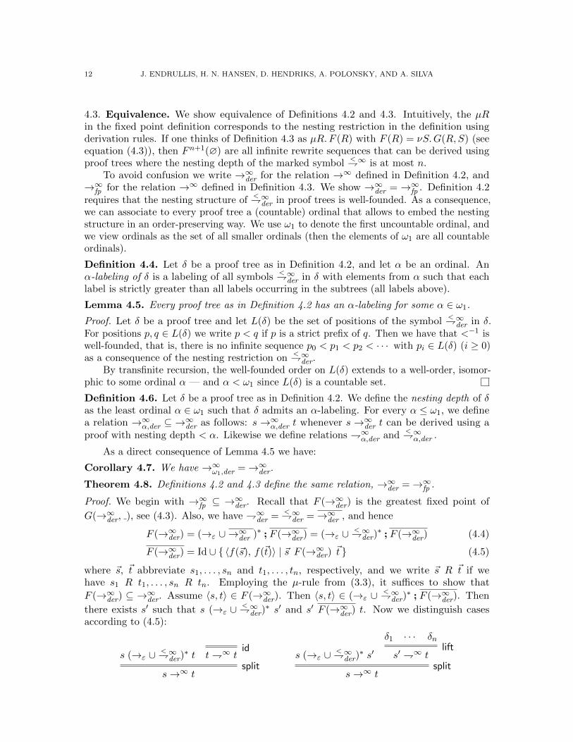
Theorem 4.8. Definitions 4.2 and 4.3 define the same relation, →∞der =→∞fp .
Proof. We begin with →∞fp ⊆ →∞der. Recall that F (→∞der) is the greatest fixed point of
G(→∞der, ), see (4.3). Also, we have ⇁∞der =<⇁∞der =→∞der , and hence
F (→∞der) = (→ε ∪ →∞der )∗ ; F (→∞der) = (→ε ∪ <⇁∞der)
∗ ; F (→∞der) (4.4)
F (→∞der) = Id ∪ { 〈f(~s), f(~t)〉 | ~s F (→∞der) ~t } (4.5)
where ~s, ~t abbreviate s1, . . . , sn and t1, . . . , tn, respectively, and we write ~s R ~t if wehave s1 R t1, . . . , sn R tn. Employing the µ-rule from (3.3), it suffices to show that
F (→∞der) ⊆ →∞der. Assume 〈s, t〉 ∈ F (→∞der). Then 〈s, t〉 ∈ (→ε ∪ <⇁∞der)
∗ ; F (→∞der). Then
there exists s′ such that s (→ε ∪ <⇁∞der)
∗ s′ and s′ F (→∞der) t. Now we distinguish casesaccording to (4.5):
s (→ε ∪ <⇁∞der)
∗ t t ⇁∞ tid
s→∞ tsplit
s (→ε ∪ <⇁∞der)
∗ s′
δ1 · · · δn
s′ ⇁∞ tlift
s→∞ tsplit

COINDUCTIVE FOUNDATIONS OF INFINITARY REWRITING AND EQUATIONAL LOGIC 13
Here, for i ∈ {1, . . . , n}, δi is the proof tree for si →∞ ti obtained from si F (→∞der) ti bycorecursively applying the same procedure.
Next we show that→∞der ⊆ →∞fp . By Corollary 4.7 it suffices to show→∞ω1,der⊆ →∞fp . We
prove by well-founded induction on α ≤ ω1 that →∞α,der ⊆ →∞fp . Since →∞fp is a fixed point
of F , we obtain →∞fp = F (→∞fp ), and since F (→∞fp ) is the greatest fixed point of G(→∞fp , ),
using the ν-rule from (3.3), it suffices to show the inclusion
(∗) →∞α,der ⊆ G(→∞fp ,→∞α,der) := (→ε ∪ →∞fp )∗ ;→∞α,der .
Thus assume that s→∞α,der t, and let δ be a proof tree of nesting depth ≤ α derivings→∞α,der t. The only possibility to derive s→∞der t is an application of the split-rule with the
premise s (→ε ∪ <⇁∞der)
∗ ; ⇁∞der t. Since s→∞α,der t, we have s (→ε ∪ <⇁∞α,der)
∗ ; ⇁∞α,der t. Letτ be one of the steps
<⇁∞α,der displayed in the premise. Let u be the source of τ and v the
target, so τ : u<⇁∞α,der v. The step τ is derived either via the id-rule or the lift-rule. The
case of the id-rule is not interesting since we then can drop τ from the premise. Thus let thestep τ be derived using the lift-rule. Then the terms u, v are of form u = f(u1, . . . , un) andv = f(v1, . . . , vn) and for every 1 ≤ i ≤ n we have ui →∞β,der vi for some β < α. Thus by
induction hypothesis we obtain ui →∞fp vi for every 1 ≤ i ≤ n, and consequently u→∞fp v.
We then have s (→ε ∪ →∞fp )∗ ; ⇁∞α,der t, and hence s G(→∞fp ,→∞α,der) t. This concludes the
proof.
5. Equivalence with the Standard Definition
In this section we prove the equivalence of the coinductively defined infinitary rewrite rela-tions→∞ from Definitions 4.2 (and 4.3) with the standard definition based on ordinal lengthrewrite sequences with metric and strong convergence at every limit ordinal (Definition 2.2).The crucial observation is the following theorem from [31]:
Theorem 5.1 (Theorem 2 of [31]). A transfinite reduction is divergent if and only if forsome n ∈ N there are infinitely many steps at depth n.
We are now ready to prove the equivalence of both notions:
Theorem 5.2. We have →∞ =→∞ord.
Proof. We write ⇁∞ord to denote a reduction →∞ord without root steps, and we write →αord
and ⇁αord to indicate the ordinal length α.
We begin with the direction→∞ord ⊆ →∞. We define a function T (and T′(<)) by guarded
corecursion [9], mapping rewrite sequences s →αord t (and s ⇁α
ord t) to infinite proof treesderived using the rules from Definition 4.2. This means that every recursive call produces aconstructor, contributing to the construction of the infinite tree. Note that the argumentsof T (and T′(<)) are not required to be structurally decreasing.

14 J. ENDRULLIS, H. N. HANSEN, D. HENDRIKS, A. POLONSKY, AND A. SILVA
We do case distinction on the ordinal α. If α = 0, then t = s and we define
T(s→0ord s) =
T′(s ⇁0ord s)
s→∞ ssplit
T′(<)(x ⇁0ord x) = x (<)⇁∞ x
id
T′(<)(f(t1, . . . , tn) ⇁0ord f(t1, . . . , tn)) =
T(t1 →0ord t1) · · · T(tn →0
ord tn)
f(t1, . . . , tn) (<)⇁∞ f(t1, . . . , tn)lift
If α > 0, then, by Theorem 5.1 the rewrite sequence s→αord t contains only a finite number
of root steps. As a consequence, it is of the form:
s = s0 s1 · · · s2n s2n+1 = t
where for every i ∈ {0, . . . , 2n}:(i) for even i, si si+1 is an infinite reduction below the root Si : si ⇁
βiord si+1, and
(ii) for odd i, si si+1 is a root step si →ε si+1,
where βi < α if i < 2n and βi ≤ α if i = 2n. For i < 2n we have βi < α since every strictprefix must be shorter than the sequence itself. We define
T(s→αord t) =
δ0 δ1 · · · δ2n
s→∞ tsplit
where, for 0 ≤ i < n,
δi =
si →ε si+1 for odd i,
T′<(Si : si ⇁βord si+1) for even i with i < 2n,
T′(Si : si ⇁βord si+1) for even i with i = 2n.
For reductions S : s ⇁αord t with α > 0 we have s = f(s1, . . . , sn) and t = f(t1, . . . , tn)
for some f ∈ Σ of arity n and terms s1, . . . , sn, t1, . . . , tn ∈ Ter∞(Σ,X ). Moreover, for every
i with 1 ≤ i ≤ n, there are rewrite sequences Si : si →≤αord ti obtained by selecting from Sthe subsequence of steps on the i-th argument. These steps are not necessarily consecutive,but selecting them nonetheless gives rise to a well-defined reduction. We define:
T′(<)(s ⇁αord t) =
T(S1 : s1 →≤αord t1) · · · T(Sn : sn →≤αord tn)
s (<)⇁∞ tlift
The obtained proof tree T(s→αord t) derives s→∞ t. To see that the requirement that
there is no ascending path through this tree containing an infinite number of symbols<⇁∞
is fulfilled, we note the following. The symbol<⇁∞ is produced by T′<(s ⇁β
ord t) which isinvoked in T(s→α
ord t) for a β that is strictly smaller than α. By well-foundedness of < onordinals, no such path exists.
We now show →∞ ⊆ →∞ord. We prove by well-founded induction on α ≤ ω1 that→∞α ⊆ →∞ord. This suffices since →∞ =→∞ω1
. Let α ≤ ω1 and assume that s→∞α t. Let δ bea proof tree of nesting depth < α witnessing s→∞α t. The only possibility to derive s→∞ tis an application of the split-rule with the premise s (→ε ∪ <
⇁∞)∗ ; ⇁∞ t. Since s →∞α t,we have s (→ε ∪ <
⇁∞α )∗ ; ⇁∞α t. By induction hypothesis we have s (→ε ∪ →∞ord)∗ ; ⇁∞α t,
and thus s→∞ord ; ⇁∞α t. We have ⇁∞α =→∞α , and consequently s→∞ord s1 →∞α t for some

COINDUCTIVE FOUNDATIONS OF INFINITARY REWRITING AND EQUATIONAL LOGIC 15
term s1. Repeating this argument on s1 →∞α t, we get s→∞ord s1 →∞ord s2 →∞α t. After niterations, we obtain
s→∞ord s1 →∞ord s2 →∞ord s3 →∞ord s4 · · · (→∞ord)−(n−1) sn (→∞α )−n t
where (→∞α )−n denotes the nth iteration of x 7→ x on →∞α .Clearly, the limit of {sn} is t. Furthermore, each of the reductions sn →∞ord sn+1 are
strongly convergent and take place at depth greater than or equal to n. Thus, the infiniteconcatenation of these reductions yields a strongly convergent reduction from s to t (thereis only a finite number of rewrite steps at every depth n).
6. Infinitary Equational Reasoning and Bi-Infinite Rewriting
6.1. Infinitary Equational Reasoning.
Definition 6.1. Let R be a TRS over Σ, and let T = Ter∞(Σ,X ). We define infinitary
equational reasoning as the relation∞= ⊆ T × T by the mutually coinductive rules:
s (←ε ∪ →ε ∪∞↽⇁)∗ t
s∞= t
s1∞= t1 · · · sn
∞= tn
f(s1, s2, . . . , sn)∞↽⇁ f(t1, t2, . . . , tn)
where∞↽⇁ ⊆ T × T stands for infinitary equational reasoning below the root.
Note that, in comparison with the rules (1.1) for∞= from the introduction, we now have
used←ε ∪ →ε instead of =R. It is not difficult to see that this gives rise to the same relation.
The reason is that we can ‘push’ non-root rewriting steps =R into the arguments of∞↽⇁.
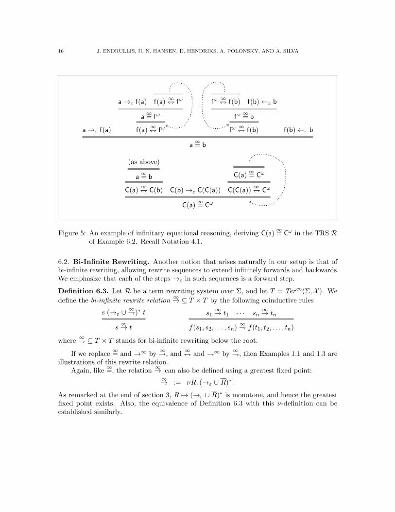
Example 6.2. Let R be a TRS consisting of the following rules:
a→ f(a) b→ f(b) C(b)→ C(C(a)) .
Then we have a∞= b as derived in Figure 5 (top), and C(a)
∞= Cω as in Figure 5 (bottom).
Definition 6.1 of∞= can also be defined using a greatest fixed point as follows:
∞= := νR. (←ε ∪ →ε ∪ R)∗ ,
where R was defined in Definition 3.1. The equivalence of these definitions can be establishedin a similar way as in Theorem 4.8. As remarked at the end of section 3, the mapR 7→ (←ε ∪ →ε ∪ R)∗ is monotone, and consequently the greatest fixed point exists.
We note that, in the presence of collapsing rules (i.e., rules ` → r where r ∈ X ),
everything becomes equivalent: s∞= t for all terms s, t. For example, having a rule f(x)→ x
we obtain that s∞= f(s)
∞= f2(s)
∞= · · · ∞= fω for every term s. This can be overcome by
forbidding certain infinite terms and certain infinite limits.
16 J. ENDRULLIS, H. N. HANSEN, D. HENDRIKS, A. POLONSKY, AND A. SILVA
a→ε f(a)
a→ε f(a) f(a)∞↽⇁ fω
a∞= fω
f(a)∞↽⇁ fω
fω∞↽⇁ f(b) f(b)←ε b
fω∞= b
fω∞↽⇁ f(b) f(b)←ε b
a∞= b
(as above)
a∞= b
C(a)∞↽⇁ C(b) C(b)→ε C(C(a))
C(a)∞= Cω
C(C(a))∞↽⇁ Cω
C(a)∞= Cω
Figure 5: An example of infinitary equational reasoning, deriving C(a)∞= Cω in the TRS R
of Example 6.2. Recall Notation 4.1.
6.2. Bi-Infinite Rewriting. Another notion that arises naturally in our setup is that ofbi-infinite rewriting, allowing rewrite sequences to extend infinitely forwards and backwards.We emphasize that each of the steps →ε in such sequences is a forward step.
Definition 6.3. Let R be a term rewriting system over Σ, and let T = Ter∞(Σ,X ). We
define the bi-infinite rewrite relation∞→ ⊆ T × T by the following coinductive rules
s (→ε ∪∞⇁)∗ t
s∞→ t
s1∞→ t1 · · · sn
∞→ tn
f(s1, s2, . . . , sn)∞⇁ f(t1, t2, . . . , tn)
where∞⇁ ⊆ T × T stands for bi-infinite rewriting below the root.
If we replace∞= and →∞ by
∞→, and∞↽⇁ and ⇁∞ by
∞⇁, then Examples 1.1 and 1.3 are
illustrations of this rewrite relation.Again, like
∞=, the relation
∞→ can also be defined using a greatest fixed point:∞→ := νR. (→ε ∪ R)∗ .
As remarked at the end of section 3, R 7→ (→ε ∪ R)∗ is monotone, and hence the greatestfixed point exists. Also, the equivalence of Definition 6.3 with this ν-definition can beestablished similarly.
COINDUCTIVE FOUNDATIONS OF INFINITARY REWRITING AND EQUATIONAL LOGIC 17
7. Relating the Notions
Lemma 7.1. Each of the relations →∞,∞→ and
∞= is reflexive and transitive. The relation
∞= is also symmetric.
Proof. Follows immediately from the fact that the relations are defined using the reflexive-transitive closure in each of their first rules.
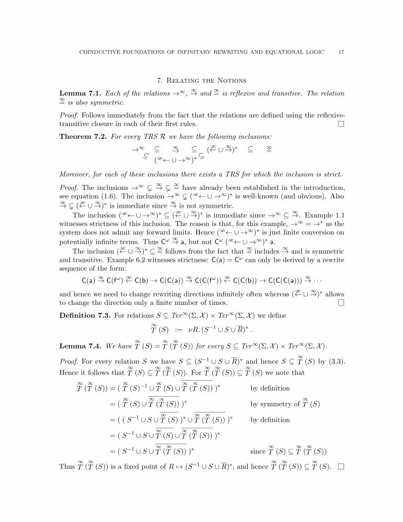
Theorem 7.2. For every TRS R we have the following inclusions:
→∞ ∞→( →∞ ∪→∞)∗
(∞→∪ ∞→)∗ ∞
=⊆ ⊆⊆ ⊆
⊆
Moreover, for each of these inclusions there exists a TRS for which the inclusion is strict.
Proof. The inclusions →∞ ( ∞→ ( ∞= have already been established in the introduction,
see equation (1.6). The inclusion →∞ ( ( →∞ ∪→∞)∗ is well-known (and obvious). Also∞→ ( (
∞→∪ ∞→)∗ is immediate since∞→ is not symmetric.
The inclusion ( →∞ ∪→∞)∗ ⊆ (∞→∪ ∞→)∗ is immediate since →∞ ⊆ ∞→. Example 1.1
witnesses strictness of this inclusion. The reason is that, for this example, →∞ =→∗ as thesystem does not admit any forward limits. Hence ( →∞ ∪→∞)∗ is just finite conversion on
potentially infinite terms. Thus Cω∞→ a, but not Cω ( →∞ ∪→∞)∗ a.
The inclusion (∞→∪ ∞→)∗ ⊆ ∞= follows from the fact that
∞= includes
∞→ and is symmetricand transitive. Example 6.2 witnesses strictness: C(a) = Cω can only be derived by a rewritesequence of the form:
C(a)∞→ C(fω)
∞← C(b)→ C(C(a))∞→ C(C(fω))
∞← C(C(b))→ C(C(C(a)))∞→ · · ·
and hence we need to change rewriting directions infinitely often whereas (∞→∪ ∞→)∗ allows
to change the direction only a finite number of times.
Definition 7.3. For relations S ⊆ Ter∞(Σ,X )× Ter∞(Σ,X ) we define∞T (S) := νR. (S−1 ∪ S ∪R)∗ .
Lemma 7.4. We have∞T (S) =
∞T (∞T (S)) for every S ⊆ Ter∞(Σ,X )× Ter∞(Σ,X ).
Proof. For every relation S we have S ⊆ (S−1 ∪ S ∪ R)∗ and hence S ⊆∞T (S) by (3.3).
Hence it follows that∞T (S) ⊆
∞T (∞T (S)). For
∞T (∞T (S)) ⊆
∞T (S) we note that
∞T (∞T (S)) = (
∞T (S)−1 ∪
∞T (S) ∪
∞T (∞T (S)) )∗ by definition
= (∞T (S) ∪
∞T (∞T (S)) )∗ by symmetry of
∞T (S)
= ( ( S−1 ∪ S ∪∞T (S) )∗ ∪
∞T (∞T (S)) )∗ by definition
= ( S−1 ∪ S ∪∞T (S) ∪
∞T (∞T (S)) )∗
= ( S−1 ∪ S ∪∞T (∞T (S)) )∗ since
∞T (S) ⊆
∞T (∞T (S))
Thus∞T (∞T (S)) is a fixed point of R 7→ (S−1 ∪ S ∪R)∗, and hence
∞T (∞T (S)) ⊆
∞T (S).

18 J. ENDRULLIS, H. N. HANSEN, D. HENDRIKS, A. POLONSKY, AND A. SILVA
It follows immediately that∞= is closed under
∞T (·).
Corollary 7.5. We have∞= =
∞T (∞=) for every TRS R.
Proof. We have∞= =
∞T (→ε) =
∞T (∞T (→ε)) =
∞T (∞=).
The work [26] introduces various notions of infinitary rewriting. We comment on the
notions that are closest to the relations∞→ and
∞= introduced in our paper. First, we note
that it is not difficult to see that∞→ (→→t where →→t is the topological graph closure of →.
The paper [26] also introduces a notion of infinitary equational reasoning with a stronglyconvergent flavour, namely:
SE(R) = (S ◦ E)?(R)
where
(i) E(R) is the equivalence closure of R, and(ii) S(R) is the strongly convergent rewrite relation obtained from (single steps) R,(iii) and f?(R) is defined as µx.R ∪ f(x).
Lemma 7.6. We have SE(→) ⊆ ∞= for every TRS R.
Proof. The following containments are immediate:
(i) → ⊆ ∞=,
(ii) E(∞=) =
∞=, and
(iii) S(∞=) ⊆
∞T (∞=) =
∞= (Corollary 7.5).
From the definition of SE(·) as a least fixed point, the claim follows.
It could be reasonable to conjecture that SE(→) and∞= coincide. We now show that
this is not the case.
Example 7.7. Consider the iTRS R consisting of the rules
c(b(x))→ a(a(x))
c(a(x))→ b(b(x))
Notice that aω∞= bω in R. One possible derivation δ of this fact is given below where
δ is the same as δ, but with all pairs mirrored and premises of the split rule are listed inreverse order. We also use that b(bω) = bω and a(aω) = aω.
a(a(aω))←εc(b(aω))
δ
c(b(aω))∞↽⇁c(b(bω))
δ
c(bω)∞↽⇁c(aω)
δ
c(a(aω))∞↽⇁c(a(bω)) c(a(bω))→εb(b(b
ω))
aω∞= bω
One does not have 〈aω, bω〉 ∈ SE(R), however. Let us sketch a proof of this. First, noticethat, for any relation R, SE(R) can alternatively be described as
SE(R) := µx.R ∪ S(E(x)) = µx.R ∪ E(x) ∪ S(x) = µx.R ∪ E(S(x)) (7.1)
This is because a prefixed point of the composition S ◦E is a prefixed point of both monotoneoperators E and S, and vice versa. We are particularly interested in the operator appearingon the right-hand side of (7.1). After a single iteration, it yields the usual concept ofinfinitary conversion in the iTRS R.

COINDUCTIVE FOUNDATIONS OF INFINITARY REWRITING AND EQUATIONAL LOGIC 19
Observe that R is in fact a string rewrite system. Being orthogonal, and having nocollapsing rules, we know that R satisfies both iCR and iSN. Therefore, infinitary conversionin R is characterized by canonical semantics S, consisting of infinitary normal forms. It iseasy to see that these are precisely
S = {w ∈ {a, b}m | m ≤ ω} t {wcn | w ∈ {a, b}∗, n ≤ ω}= {wcn | w ∈ {a, b}m,m+ n ≤ ω}
It is a curious fact that E(S(·)) does not yet stabilize at (=S), the equality of infinitarynormal forms. But it does stabilize after one more iteration — without relating aω and bω.
To see this, consider a sequence of =S-steps
s0 →∞ · →∞ s1 →∞ · →∞ s2 →∞ · · · with limn→∞
sn = s∞ (7.2)
By infinitary rewriting theory, for each n, we can find standard, ω-compressed reductions
ρn : sn →∞ s := NF∞(s0) ∈ S (7.3)
Let us say that a finite prefix w ≤ s is stable if we can find a number N , a prefix v ≤ s∞,and a reduction ν : v →∗ w such that, for all n ≥ N :
– sn = vs′n– ρn factors as ρn = ν ◦ ρ′n, where ρ′n : s′n → s′ and s = ws′.
If every prefix of s is stable, then it is easy to see that s∞ →∞ s; then the infiniteconversion (7.2) yields no new pairs in SE(R).
Otherwise, there is a maximal stable prefix w — which may or may not be empty.Fixing this w = wmax , with respective N , v, and ν, we find that
– s = ws′, s∞ = vs′∞, ν : v → w;– s′N →∞ · →∞ s′N+1 →∞ · · ·, with limn→∞ s
′n = s′∞;
– s′n →∞ s′ for n ≥ N ;
We claim that s′∞ = cω. For suppose s′∞ ∈ {ckxu | k ≥ 0, x ∈ {a, b}, u ∈ {a, b, c}≤ω}.After k steps of outermost reduction, the outermost letter becomes y ∈ {a, b}, and there isno longer a redex present at the root. By continuity of the sequence {s′n}, this even happensat each n ≥M , for some M ≥ N . But now y becomes a stable prefix of s′, and wy a stableprefix of s — contradicting maximality of w. So s′∞ = cω. Now, unless s′ = cω as well,trivializing the whole thing, the reductions ρ′n must be non-trivial, yielding subterms of formaa(x) or bb(x). Then s′ has a prefix resulting from a reduction of a term of form ckau orckbu to normal form — for arbitrarily large k. A cursory examination of the rules revealsthat the only two possibilities for such prefixes are a(ab)k and b(ba)k. Since the k indeed isunbounded as s′n → s′∞, we conclude that s′ ∈ {a(ab)ω, b(ba)ω}.
Thus, the only pairs added to (=S) by the operator S(·) are those of the form 〈wα, vcω〉,where v →∗ w and α ∈ {a(ab)ω, b(ba)ω}. The equivalence generated by these relationscorresponds to infinitary conversion in the augmented iTRS:
R+ := R∪
{a(ab)ω → cω
b(ba)ω → cω
Let us denote this conversion by =S+ . It remains to show that SE(=S+) coincides with=S+ . We proceed as before, starting with a chain of R+-conversions
s0 →∞ · →∞ s1 →∞ · →∞ s2 →∞ · · · with limn→∞
sn = s∞ (7.4)

20 J. ENDRULLIS, H. N. HANSEN, D. HENDRIKS, A. POLONSKY, AND A. SILVA
We remark that R+ is still confluent, owing to lack of overlap.Even though compression fails due to the presence of rules with infinite left sides, this
failure happens to be completely innocuous: if any of these rules are ever used in a reductionsequence, they will replace an infinite part of the term by a normal form which cannotinteract with anything — and the finite prefix which remains is strongly normalizing (sinceR+ is finitarily SN). In particular, for any R+-reduction ρ : u →∞ u′, the following areequivalent:
– ρ cannot be compressed to length ω;– ρ factors as u→∞ wα→ wcω, where α ∈ {a(ab)ω, b(ba)ω} and u→∞ wα is is an infinite
reduction.
We thus again obtain standard, (ω + 1)-compressed reductions
ρn : sn →∞ s := NF∞(s0) ∈ S (7.5)
If it so happens that, no reduction ρn fires any of the new rules, then it is evident that(s, s∞) is already included in =S+ . Otherwise, if one of the new rules is ever fired, thens = wcω. If t is any term, and ρ is a reduction from t to a normal form of the shape wcω,then ρ factors as ρf ◦ ρi ◦ ρ!, where
– t = t0ti;– ρf : t0 →∗ w;– ρi : ti →∞ α are reductions in R, where α ∈ {a(ab)ω, b(ba)ω};– ρ! : α→ cω.
Applying this observation for each ρn from (7.5), we conclude that the initial part ρfnmust eventually stabilize (due to stabilization of prefixes as sn
n→∞−→ s∞). For the samereason, we have that ρ!
n must eventually settle on one of the two new rules, with the targetof ρi converging to its left side. The remaining reductions ρi, being pure R-reductions, arecovered by our earlier analysis, and so we conclude that s∞ = s0
∞si∞, with s0
∞=S+w, andsi∞=S+c
ω.Finally, let us remark why it suffices to consider limits of length ω. This is settled by
induction on the sequence length β.As decisively settled in TeReSe, a strongly convergent sequence is necessarily of at-most-
countable length β.If β is a successor ordinal, then we conclude by finite induction from the greatest limit
ordinal less than β.Otherwise, β will be a limit ordinal, and we shall be able to produce a sequence
s0, sβ(1), sβ(2), . . . as before, with sβ(i) →∞ · →∞ s0.The same analysis applies, and we deduct that sβ →∞R+ NF(s0).
8. Correspondence of Proof Trees and Rewrite Sequences
In this section, we investigate the correspondence between ordinal-indexed rewrite sequencesand coinductive proof trees. We define a correspondence relation that makes precise when arewrite sequence is represented by a certain proof tree. In general, this correspondence is amany-to-many relation: a proof tree represents a class of rewrite sequences, and a rewritesequence can be represented by different proof trees.
We then define canonical proof trees for →∞ in such a way that every ordinal-indexedrewrite sequence has a unique representative among the canonical proof trees. More precisely,

COINDUCTIVE FOUNDATIONS OF INFINITARY REWRITING AND EQUATIONAL LOGIC 21
there is a many-to-one correspondence between rewrite sequences and canonical proof trees.To characterise the class of rewrite sequences represented by the same canonical prooftree, we introduce a notion of equivalence on infinitary rewrite sequences, called parallelpermutation equivalence. Thereby two rewrite sequences are considered equivalent if theydiffer only in the order of steps in parallel subtrees.
Notation 8.1. For a rewrite sequence S : s0 →αR sα consisting of steps (sβ → sβ+1)β<α
arising from the application of the rule `β → rβ with substitution σβ at position pβ,respectively, we introduce the following notation
rul(S, β) = `β → rβ
pos(S, β) = pβ
sub(S, β) = σβ
for every β < α.
8.1. The Correspondence Relation. Assume that we have a term f(s1, . . . , sn) andrewrite sequences on the direct subterms S1 : s1 →α1 t1, . . . , Sn : sn →αn tn. As theserewrite sequences occur in parallel subterms, any interleaving of them gives rise to a rewritesequence f(s1, . . . , sn) →β f(t1, . . . , tn). The following definition introduces the notion ofinterleaving on the basis of a monotonic bijective embedding of the disjoint union α1] . . .]αninto β.
Definition 8.2. Let f ∈ Σ of arity n. Let Si : si →αi ti be rewrite sequences of length αifor every i ∈ { 1, . . . , n }. A rewrite sequence T : f(s1, . . . , sn)→β f(t1, . . . , tn) of length βis called an interleaving of S1, . . . , Sn with root f if there exists a bijection
ξ : ({1} × α1 ∪ . . . ∪ {n} × αn)→ β
such that for every i ∈ { 1, . . . , n } and every γ < αi we have:
(i) pos(T, ξ(i, γ)) = i · pos(Si, γ) (corresponding position in the i-th argument),(ii) rul(T, ξ(i, γ)) = rul(Si, γ) (same rule),(iii) sub(T, ξ(i, γ)) = sub(Si, γ) (same substitution), and(iv) for every γ′ < γ it holds that ξ(i, γ′) < ξ(i, γ) (monotonic embedding).
The following definition introduces the correspondence between coinductive proof treesand ordinal-indexed rewrite sequences.
Definition 8.3. Let R be a term rewriting system. We define the correspondence relationbetween proof trees (with respect to Definition 4.2) and ordinal-indexed rewrite sequencesas the largest relation such that the following conditions hold:
(i) A proof tree of the form
δ1 δ2 · · · δn
s→∞ tsplit
corresponds to a rewrite sequence S : s →α t if S is the concatenation of rewritesequences S1, . . . , Sn such that δi corresponds to Si for every i ∈ { 1, . . . , n }.
(ii) A proof tree of the form s→ε t only corresponds to the rewrite sequence s→ε t.

22 J. ENDRULLIS, H. N. HANSEN, D. HENDRIKS, A. POLONSKY, AND A. SILVA
(iii) A proof tree of the form
δ1 δ2 · · · δn
f(s1, s2, . . . , sn) (<)⇁∞ f(t1, t2, . . . , tn)lift
corresponds to a rewrite sequence S : s→α t if S is an interleaving of rewrite sequencesS1, . . . , Sn with root f such that the proof tree δi corresponds to the rewrite sequenceSi for every i ∈ { 1, . . . , n }.
(iv) A proof tree of the form
s (<)⇁∞ sid
only corresponds to the empty rewrite sequence s→0 s.
Remark 8.4. Note that a proof tree corresponds to more than one rewrite sequence if andonly if it contains an application of the lift-rule with (at least) two premises that do notcorrespond to empty rewrite sequences. The lift-rule introduces choice in the ‘construction’of the rewrite sequence by allowing for an arbitrary interleaving of the rewrite sequences onthe arguments.
The following example illustrates that a proof term can correspond to an infinite numberof ordinal-indexed rewrite sequences.
Example 8.5. We consider the proof trees in Figures 3 and 4:
(i) The proof tree for a→∞ Cω corresponds to the only rewrite sequence a→ω Cω.(ii) The proof tree for b→∞ Cω corresponds to the only rewrite sequence b→ω Cω.(iii) The proof tree for f(a, b)
<⇁∞ f(Cω,Cω) corresponds to all possible interleavings of
a→ω Cω and b→ω Cω applied to the respective subterms f(a, b). Note that there arecontinuum many rewrite sequences that all have length ω or ω · 2.
The next example shows that some rewrite sequences can be represented by multiple prooftrees.
Example 8.6. There are multiple proof trees for the rewrite sequence a→ω Cω, for examplethe proof trees shown in Figures 3 and 6.
a→ε C(a)
a→ε C(a)
a→∞ C(a)
C(a) ⇁∞ C(C(a))
a→∞ Cω
C(a) ⇁∞ Cω
C(a)→∞ Cω
C(C(a)) ⇁∞ Cω
a→∞ Cω
Figure 6: A second proof tree for a→∞ Cω.

COINDUCTIVE FOUNDATIONS OF INFINITARY REWRITING AND EQUATIONAL LOGIC 23
Example 8.7. Let R consist of the rule f(x) → g(x). Figures 7 and 8 show proof treescorresponding to rewrite sequences fω →ω gω. The proof tree in Figure 7 corresponds to therewrite sequence
fω → g(fω)→ g(g(fω))→ · · · →ω gω ,
and the proof tree in Figure 8 corresponds to
fω → g(fω)→ g(f(g(fω)))→ g3(fω)→ g4(fω)→ g5(fω)→ · · · →ω gω .
Note that, by Remark 8.4, these rewrite sequences are unique. Both proof trees correspondto precisely one rewrite sequence since they do not contain applications of the lift-rule (ruleswith conclusion ⇁∞) with multiple premises.
fω →ε g(fω)
fω →∞ gω
g(fω) ⇁∞ gω
fω →∞ gω
Figure 7: A proof tree for fω → g(fω)→ g(g(fω))→ · · · →ω gω.
fω →ε g(fω)
fω →ε g(fω)
fω →∞ g(fω)
fω ⇁∞ f(g(fω)) f(g(fω))→ε g(g(fω))
Figure 7
fω →∞ gω
g(fω) ⇁∞ gω
g(fω)→∞ gω
g(g(fω)) ⇁∞ gω
fω →∞ gω
g(fω) ⇁∞ gω
fω →∞ gω
Figure 8: A proof tree for fω → g(fω)→ g(f(g(fω)))→ g3(fω)→ g4(fω)→ · · · →ω gω.
8.2. Canonical Proof Trees and Parallel Permutation Equivalence. In order to havea unique proof tree for every ordinal-indexed rewrite sequence, we introduce ‘canonical’proof trees for →∞. We show that the correspondence of canonical proof trees and rewritesequences is a one-to-many relationship, and we characterise the class of rewrite sequencesrepresented by a canonical proof tree in terms of ‘parallel permutation equivalence’.

24 J. ENDRULLIS, H. N. HANSEN, D. HENDRIKS, A. POLONSKY, AND A. SILVA
Definition 8.8. A proof tree for →∞ is called canonical if
(i) every application of the split rule is an instance of the canonical split rule
s (<⇁∞ ;→ε)
∗ ; ⇁∞ t
s→∞ tcanonical split , and
(ii) every application of the id rule is an instance of
x (<)⇁∞ xcanonical id
In contrast with the split rule from Definition 4.2, the canonical split rule replaces
(<⇁∞ ∪ →ε)
∗ by (<⇁∞ ;→ε)
∗ .
Thereby the canonical form enforces that<⇁∞ and →ε alternate.
The canonical id rule replaces
s (<)⇁∞ s by x (<)⇁∞ x .
Thereby it enforces unique proof trees for empty rewrite sequences (using rules lift andcanonical id).
Definition 8.9. Let p, q ∈ N∗ be positions. We define
(i) p ≤ q if pr = q for some r ∈ N∗,(ii) p ‖ q if p 6≤ q and q 6≤ p.
If p ‖ q, then we say that p and q are parallel (to each other).
Recall that we consider ordinals α to be the set of all smaller ordinals: α = {β | β < α}.This allows us to speak about functions f : α→ β.
Definition 8.10. Let R be a term rewriting system. Let S : s→∞R t1 and T : s→∞R t2 bestrongly convergent rewrite sequences of length α and β, respectively.
The rewrite sequence S is called parallel permutation equivalent to T if there exists abijection f : α→ β such that
(i) rul(S, γ) = rul(T, f(γ)) and pos(S, γ) = pos(T, f(γ)) for every γ < α, and(ii) pos(S, γ1) ‖ pos(S, γ2) whenever γ1 < γ2 < α and f(γ1) > f(γ2).
Observe that, the bijective mapping f : α → β defines a permutation of the steps in thesequence S. The condition (i) guarantees that the step indexed by γ in S corresponds to thestep indexed by f(γ) in T as follows: both steps must arise from the same rule applied atthe same position. The condition (ii) ensures that steps that have been permuted (changedtheir relative order in the sequence), arise from contractions at parallel positions.
In the following definition we select a subsequence of the steps of T that corresponds to(the permutation of) a prefix of S. For this purpose, we consider a step to be the applicationof a certain rule at a certain position. We do not take into account the source and the targetof the steps as these may change due to preceding steps being dropped (not selected).
Definition 8.11. Let S : s0 →αR sα and T : t0 →β
R tβ be parallel permutation equivalentwith respect to the bijection f : α→ β. Let κ ≤ α, and define S′ as the prefix of S of lengthκ. We define the permutation of S′ with respect to f as the rewrite sequence obtained fromT by selecting the subsequence of steps at indexes γ < β for which f−1(γ) < κ.
COINDUCTIVE FOUNDATIONS OF INFINITARY REWRITING AND EQUATIONAL LOGIC 25
As dropping (not selecting) a step changes all subsequent terms in the sequence, weneed to show that the selected steps still form a rewrite sequence (the rules are applicable atthe designated positions).
Proof of well-definedness of Definition 8.11. To prove that the selected subsequence of stepsfrom T forms a rewrite sequence, we show that every non-selected (dropped) step is parallelto all subsequent selected steps. As a consequence, the dropped steps do not influencethe applicability of the selected steps. Let us consider a step that is dropped, that isγ < β with f−1(γ) ≥ κ, and a subsequent step that is selected, γ′ with γ < γ′ < β andf−1(γ′) < κ. From parallel permutation equivalence of S and T it follows immediately thatpos(T, γ) ‖ pos(T, γ′) since f−1(γ′) < κ ≤ f−1(γ) and γ < γ′.
Lemma 8.12. Let S : s0 →αR sα and T : t0 →β
R tβ be parallel permutation equivalent withrespect to the bijection f : α→ β. Every prefix S′ of S is parallel permutation equivalent tothe permutation of S′ with respect to f .
Proof. Follows immediately from parallel permutation equivalence of the rewrite sequencesS and T together with Definition 8.11 since the order of the selected steps is preserved (bothfrom S to S′ as well as from T to the subsequence of selected steps of T ).
The following lemma states that parallel permutation equivalent sequences converge tothe same target term.
Lemma 8.13. If the rewrite sequences S : s0 →αR sα and T : t0 →β
R tβ are parallelpermutation equivalent, then we have sα = tβ.
Proof. We prove the claim by induction on α. Let S : s0 →αR sα and T : t0 →β
R tβ berewrite sequences that are parallel permutation equivalent. Let f : α→ β be such that theconditions of Definition 8.10 are fulfilled. We distinguish cases for α:
(i) If α = 0, it follows that β = 0. Then s0 = t0 by definition of parallel permutationequivalence (the starting terms of the reductions must be equal).
(ii) If α is a successor ordinal α = α′ + 1, we proceed as follows.
Let S′ be the prefix s→α′ sα′ of S of length α′. In other words, S′ is the rewritesequence obtained from S by dropping the last step sα′ → sα.
Let T ′ be the permutation of S′ with respect to f . So, T ′ is the rewrite sequences→β′ uβ′ with β′ ≤ β obtained from T by dropping the step tf(α′) → tf(α′)+1. Let
(`→ r) = rul(T, f(α′)) p = pos(T, f(α′)) σ = sub(T, f(α′))
Recall that the step tf(α′) → tf(α′)+1 can be dropped from T as its position is parallelto the positions of all subsequent steps in T : pos(T, f(α′)) ‖ pos(T, γ) for every γ withf(α′) < γ < β. From this fact it also follows that
uβ′ |p = tf(α′)|p = `σ tβ|p = tf(α′)+1|p tβ = uβ′ [rσ]p (8.1)
Observe that S′ is shorter than S as we have removed the last step. In contrast, thelength of T ′ may be less or equal to the length of T . For example, dropping the 5thstep from an ω-long sequence does not decrease its length.
From parallel permutation equivalence of S and T , it follows by Lemma 8.12 that S′
and T ′ are parallel permutation equivalent. By induction hypothesis, we may concludethat sα′ = uβ′ . From (8.1) it follows that
sα′ |p = `σ sα = sα′ [rσ]p

26 J. ENDRULLIS, H. N. HANSEN, D. HENDRIKS, A. POLONSKY, AND A. SILVA
since rul(S, α′) = rul(T, f(α′)) = `→ r and pos(S, α′) = pos(T, f(α′)) = p. Then
sα = sα′ [rσ]p = uβ′ [rσ]p = tβ .
(iii) Assume α is a limit ordinal. We use s =n t to denote that the terms s and t coincideup to depth n. For sα = tα it suffices to show that sα =n tα for every n ∈ N.
Let n ∈ N be arbitrary. By strong convergence of S there exists a strict prefix S′
of S that contains all steps of S at depth ≤ n. So, if κ is the length of S′, then allsteps in S at index an γ ≥ κ have depth > n. Let T ′ be the permutation of S′ withrespect to f . By Lemma 8.12, S′ and T ′ are permutation equivalent, and by inductionhypothesis, they have the same final term, say final term u. As all steps in S after thelast step of S′ are at depth > n we obtain u =n sα. Likewise, we get u =n tβ since T ′
contains all steps of T that are at depth ≤ n. Hence sα =n tβ.
This concludes the proof.
Proposition 8.14. Parallel permutation equivalence is an equivalence relation.
Proof. We prove reflexivity, symmetry and transitivity:
(a) Reflexivity. Parallel permutation equivalence of a rewrite sequence S : s→α t to itselfis witnessed by choosing f as the identity function on α in Definition 8.10; then bothconditions in the definition are trivially fulfilled.
(b) Symmetry. Let S : s →α t be parallel permutation equivalent to T : s →β t withwitnessing bijection f : α → β. Then parallel permutation equivalence of T to S iswitnessed by f−1; we check both conditions of Definition 8.10:
(i) rul(T, γ) = rul(T, f(f−1(γ))) = rul(S, f−1(γ)) andpos(T, γ) = pos(T, f(f−1(γ))) = pos(S, f−1(γ)) for every γ < β
(since f−1(γ) < α)(ii) We have
γ1 < γ2 < β with f−1(γ1) > f−1(γ2)
⇐⇒ f−1(γ2) < f−1(γ1) < α with f(f−1(γ2)) = γ2 > γ1 = f(f−1(γ1))
Hence pos(T, γ1) ‖ pos(T, γ2) whenever γ1 < γ2 < β and f−1(γ1) > f−1(γ2).(c) Transitivity. Let S : s →α t be parallel permutation equivalent to T : s →β t and
T : s →β t parallel permutation equivalent to U : s →δ t witnessed by bijectionsf : α→ β and g : β → δ, respectively. Then parallel permutation equivalence of S to Uis witnessed by g ◦ f ; we check both conditions of Definition 8.10:
(i) rul(S, γ) = rul(T, f(γ)) = rul(U, g(f(γ))) andpos(S, γ) = pos(T, f(γ)) = pos(U, g(f(γ))) for every γ < α, and
(ii) Assume that γ1 < γ2 < α with g(f(γ1)) > g(f(γ2)). Then either f(γ1) > f(γ2) orf(γ1) < f(γ2) ∧ g(f(γ1)) > g(f(γ2)). In the former case, pos(S, γ1) ‖ pos(S, γ2)follows from parallel permutation equivalence of S to T . In the latter case, itfollows from parallel permutation equivalence of T to U .
The following lemma implies that the witnessing function f in the definition of parallelpermutation equivalence is unique (for fixed rewrite sequences S and T ).
COINDUCTIVE FOUNDATIONS OF INFINITARY REWRITING AND EQUATIONAL LOGIC 27
Lemma 8.15. Let S : s →α t and T : s →β t be rewrite sequences. Let α′ ≤ α and letf : α′ → β be an an injective function with the properties
(i) rul(S, γ) = rul(T, f(γ)) and pos(S, γ) = pos(T, f(γ)) for every γ < α′, and(ii) pos(S, γ1) ‖ pos(S, γ2) whenever γ1 < γ2 < α′ and f(γ1) > f(γ2).(iii) pos(T, γ1) ‖ pos(T, γ2) whenever γ1 < γ2 < β, γ1 is not in the image of f , but γ2 is,
Then f is unique with these properties ( for fixed S, T , α′).Moreover, among the ordinals ≤ α, there exists a largest ordinal α′ such that a function f
with these properties exists.
Before we prove the lemma, let us give some intuition for the conditions (i)–(iii). Item (i)ensures that f correctly embeds S into T in the sense it respects redex position and theapplied rule. Condition (ii) guarantees that f only swaps steps that are at parallel positions.Finally, condition (iii) requires that steps in T that are not in the image of f must be parallelto all subsequent steps in T that are in the image of f .
Proof of Lemma 8.15. We prove uniqueness of f by induction on α′
The base case α′ = 0 is trivial.For α′ a successor ordinal, α′ = α′′+1, we argue as follows. Let f, g : α′ → β be injective
functions fulfilling the properties (i)–(iii). Then by induction hypothesis, the functions f |α′′and g|α′′ coincide. Assume, for a contradiction, f(α′′) 6= g(α′′). Without loss of generalitywe may assume f(α′′) < g(α′′). Then f(α′′) < g(α′′) < β and f(α′′) is not in the image of g,but g(α′′) is. However, pos(T, f(α′′)) = pos(S, α′′) = pos(T, g(α′′)), contradicting property(iii) for the function g. Hence f and g coincide.
Let α′ be a limit ordinal and let f, g : α′ → β be injective functions fulfilling theproperties (i)–(iii). Assume, for a contradiction, that f(α′′) 6= g(α′′) for some α′′ < α′.However, we have that α′′ + 1 < α′ since α′ is a limit ordinal. By induction hypothesis weobtain f |α′′+1 coincides with g|α′′+1. Thus f(α′′) = g(α′′), contradicting our assumption.Hence, f and g coincide. This concludes the proof of uniqueness of f .
We write P (α′) if there exists an injective function f : α′ → β with properties (i)–(iii).It remains to be shown that there exists a largest ordinal α′ ≤ α for which P (α′) holds.Let ξ be the supremum (union) of all ordinals ξ′ ≤ α for which P (ξ′); note that this set isnon-empty since always P (0) holds. If P (ξ), then ξ is the largest of these ordinals. Thusassume ¬P (ξ). Then ξ is a limit ordinal. Note that ξ′′ < ξ′ and P (ξ′) imply P (ξ′′). Asa consequence we have P (ξ′) for every ξ′ < ξ. As the length of every rewrite sequence iscountable [35], it follows that α and thus ξ are countable. Every countable limit ordinalhas cofinality ω. Thus there exist ordinals ξ1 < ξ2 < ξ3 < . . ., each of which < ξ, such thatξ =
⋃{ ξi | i ∈ N }. Then P (ξi) for every i ∈ N. For every i ∈ N, there exists an injective
function fi : ξi → β fulfilling properties (i)–(iii) for α′ = ξi. From the uniqueness (shownabove), it follows that fi coincides with fj |ξi for every i < j. As a consequence, we candefine f : ξ → β by
f(ξ′) = fi(ξ′) whenever i ∈ N and ξ′ < ξi .
We claim that f is injective and has the properties (i)–(iii) and hence P (ξ) holds; contradictingthe above assumption. Injectivity and property (i) are immediate. Property (ii) follows fromthe fact that for γ1 < γ2 < ξ there exists i ∈ N such that γ1, γ2 < ξi (since ξ is the supremumof the ξi’s). Then fi fulfilling property (ii) for γ1, γ2 implies f fulfilling property (ii) for γ1, γ2.Analogously, property (iii) follows from the following observation: whenever γ1 < γ2 < β, ifγ2 is in the image of f and γ1 is not, then there exists some i such that γ2 is in the image of

28 J. ENDRULLIS, H. N. HANSEN, D. HENDRIKS, A. POLONSKY, AND A. SILVA
fi (because f is the union of all fj), while γ1 is not (since the image of f contains that of allfj).
Lemma 8.16. Let S : s→α t be a rewrite sequence. Then S is of the form
S = S1 ; S2 ; S3 ; · · · ; S2n+1
for some n ∈ N such that for every i ∈ { 1, . . . , 2n } we have:
(i) for odd i, Si : si →α si+1 is a reduction below the root,(ii) for even i, Si : si →ε si+1 is a root step.
If S is parallel permutation equivalent to T : s→β t, then T is of the form:
T = T1 ; T2 ; T3 ; · · · ; T2n+1
such that Si is parallel permutation equivalent to Ti for every i ∈ { 1, . . . , 2n+ 1 }.
Proof. From the definition of parallel permutation equivalence, it follows that
(?) no steps can swap the order with a root step.
As a consequence, T contains the same root steps as S, in the same order. Hence T is of theform T = T1 ; T2 ; T3 ; · · · ; T2n+1 such that for every i ∈ { 1, . . . , 2n } we have:
(i) for odd i, Ti : ti →α ti+1 is a reduction below the root,(ii) for even i, Ti : ti →ε ti+1 is a root step, the same as Si.
From (?) it moreover follows that Si is parallel permutation equivalent to Ti for everyi ∈ { 1, . . . , 2n+ 1 }. The reason is that there cannot be a step s ∈ Si with f(s) ∈ Tj wherei, j are odd and j 6= i. For otherwise, this would imply a swap of s with respect to the rootstep Si+1 (if i < j) or the root step Si−1 (if i > j).
The next definition extracts the order in which certain rule applications occur in arewrite sequence. A rule application is formally a pair 〈ρ, p〉 ∈ R×N∗ consisting of a rewriterule and a position. A step in a rewrite sequence of length α is a triple 〈β, ρ, p〉 where β < αis an index and 〈ρ, p〉 is a rule application. Given a rewrite sequence S, consider the sequenceof rule applications that take place at each step in S. We are interested in the subsequenceof all those 〈ρ, p〉 that fall in a given set P ⊆ R× N∗.
Definition 8.17. Let S : s→α t be a rewrite sequence. The rule application sequence of Sis the sequence rulapp(S) : α → R× N∗ given by rulapp(S)(β) = 〈rul(S, β), pos(S, β)〉 forall β < α. Given a set P ⊆ R× N∗ of rule applications, we define the P -projection of S asthe subsequence projP (S) of rulapp(S) obtained by picking all rule applications in P .
In other words, projP (S) is a function projP (S) : β → P for some ordinal β ≤ α togetherwith an embedding f : β → α such that:
(i) f is an embedding: projP (S)(γ) = 〈 rul(S, f(γ)), pos(S, f(γ)) 〉 for every γ < β,(ii) f is increasing: f(γ1) < f(γ2) whenever γ1 < γ2 < β, and(iii) f selects all rule applications in P : for all steps 〈γ, rul(S, γ), pos(S, γ) 〉 in S, if
〈 rul(S, γ), pos(S, γ) 〉 ∈ P then γ is in the image of f .
We say that rewrite sequences S1 and S2 have the same order of rule applications inP ⊆ R× N∗ if projP (S1) = projP (S2) (here we mean point-wise equality).
It should be clear that for given S and P , projP (S) is well-defined.
COINDUCTIVE FOUNDATIONS OF INFINITARY REWRITING AND EQUATIONAL LOGIC 29
Example 8.18. Consider a rewrite system with rules (ρ1) a(x) → a(a(x))(ρ2) b(x) → b(b(x))(ρ3) f(x, y) → f(a(c), b(c))
Then we can rewrite
S : f(a(c), b(c)) → f(a(a(c)), b(c)) using 〈ρ1, 0〉→ f(a(a(a(c))), b(c)) using 〈ρ1, 0〉→ f(a(a(a(c))), b(b(c))) using 〈ρ2, 1〉→ f(a(c), b(c)) using 〈ρ3, ε〉→ f(a(c), b(b(c))) using 〈ρ2, 1〉→ f(a(a(c)), b(b(c))) using 〈ρ1, 0〉
Taking P = {〈ρ1, 0〉, 〈ρ2, 1〉}, we get that projP (S) = 〈ρ1, 0〉, 〈ρ1, 0〉, 〈ρ2, 1〉, 〈ρ2, 1〉, 〈ρ1, 0〉,and, in particular, β = 5.
The following lemma states, for a given proof tree, the order of non-parallel ruleapplications is the same in every rewrite sequence corresponding to the proof tree.
Lemma 8.19. Let δ be a proof tree (Definition 4.2) and let P ⊆ R× N∗ be a set of ruleapplications such that for every 〈ρ1, p1〉, 〈ρ2, p2〉 ∈ P we have p1 ∦ p2. If rewrite sequences Sand T both correspond to δ, then projP (S) = projP (T ).
Proof. It suffices to consider the case that P consists of at most 2 elements since:
projP (S) = projP (T ) ⇐⇒ ∀Q ⊆ P. (|Q| ≤ 2 =⇒ projQ(S) = projQ(T )) .
We prove that for all proof trees δ and all P ⊆ R× N∗ with |P | ≤ 2, if rewrite sequencesS and T correspond to δ, then projP (S) = projP (T ). So let δ, S, T, P be as stated, andassume that P = {〈ρ1, p1〉, 〈ρ2, p2〉}; we allow 〈ρ1, p1〉 = 〈ρ2, p2〉. Without loss of generality,we assume that p1 ≤ p2. The proof is by well-founded induction on the length of p2. Firstwe note that if δ is a single root step or a single application of id, the result is immediate.
Base case: Here we have p2 = p1 = ε which means that P contains only root stepapplications. We distinguish cases according to the root of δ. If the root of δ is obtainedfrom a split-application, then the root steps in S and T must occur in the same order, henceprojP (S) = projP (T ). In case the root of δ is obtained from a lift-application, then S and Tcannot contain any root steps, hence we are also done.
Induction step: Assume that p2 = ip′2 and define
P ′ =
{{〈ρ2, p
′2〉}, if p1 = ε
{〈ρ1, p′1〉, 〈ρ2, p
′2〉}, if p1 = ip′1
By induction, we may assume that the property holds for the set of rule applications P ′.For (ρ, p) ∈ (R× N∗), we define i · (ρ, p) = (ρ, ip). For functions h : β → R× N∗, we
define (i · h) : β → R× N∗ by by (i · h)(γ) = i · h(γ).We distinguish cases for the shape of δ. If δ is of the form:
δ1 : s1 →∞ t1 δ2 : s2 →∞ t2 · · · δn : sn →∞ tn
f(s1, . . . , sn) (<)⇁∞ f(t1, . . . , tn)lift
then S, respectively T , is an interleaving of rewrite sequences S1, . . . , Sn, respectivelyT1, . . . , Tn, corresponding to δ1, . . . , δn. In particular, Si : si →∞ ti and Ti : si →∞ ticorrespond to δi. Since S cannot contain root steps, we have that 〈ρ1, ε〉 is not in theimage of projP (S), so if p1 = ε then projP (S) = i · projP ′(Si). If p1 = ip′i, then all

30 J. ENDRULLIS, H. N. HANSEN, D. HENDRIKS, A. POLONSKY, AND A. SILVA
ρ1- and ρ2-applications in P are on the i’th subterm, and since interleaving preservesorder of steps in this subterm, we again have that projP (S) = i · projP ′(Si). Similarly,projP (T ) = i · projP ′(Ti). Now, projP (S) = projP (T ) follows from the induction hypothesis.
If δ is of the formδ1 δ2 · · · δn
s→∞ tsplit
then S, respectively T , is a concatenation of S1, . . . , Sn, respectively T1, . . . , Tn, correspondingto the trees δ1, . . . , δn. Hence it suffices to show that projP (Si) = projP (Ti) for all i = 1, . . . , n.For all δi’s that are a single node or an id-application, this holds. The remaining δi’s musthave a root that is obtained from a lift-application, and the result now follows from thelift-case.
Next, we characterise the correspondence of canonical proof trees and rewrite sequences.
Theorem 8.20. We have the following facts about canonical proof trees:
(i) Every rewrite sequence corresponds to precisely one canonical proof tree.
(ii) Rewrite sequences S : s0 →αR sα and T : t0 →β
R tβ are represented by the samecanonical proof tree if and only if they are parallel permutation equivalent.
Proof. First, note that every rewrite sequence corresponds to a canonical proof tree. Thisfollows by an inspection of the proof of Theorem 5.2: for every rewrite sequence S : s→α t,the proof tree T(S) is canonical and corresponds to S.
Second, we show that canonical proof trees coincide if they correspond to rewritesequences that are parallel permutation equivalent. As a direct consequence, we obtain thatevery rewrite sequence corresponds to precisely one canonical proof tree, establishing (i).
Notation: For a strongly convergent rewrite sequence R : s →αord t, we write TR to
denote an arbitrary canonical proof tree TR : s →∞ t corresponding to R. Note that, apriori, the tree TR can be different from T(R). If R is a rewrite sequence below the root,
then we moreover write T′(<)R for a canonical proof tree T
′(<)R : s (<)⇁∞ t corresponding to R.
Let S : s →αord t and T : s →β
ord t be rewrite sequences that are parallel permutationequivalent. We show that TS = TT by coinduction, that is: if S and T are parallelpermutation equivalent, then TS and TT have the same root and all subtrees arise againfrom parallel permutation equivalent rewrite sequences. As S and T are parallel permutationequivalent, from Lemma 8.16 it follows that S and T are of the forms:
S = S1 ; S2 ; S3 ; · · · ; S2n+1
T = T1 ; T2 ; T3 ; · · · ; T2n+1(8.2)
for some n ∈ N such that for every i ∈ { 1, . . . , 2n+ 1 } we have:
(a) for odd i, Si and Ti are reductions below the root,(b) for even i, Si and Ti are a root steps, and(c) Si is parallel permutation equivalent to Ti for every i ∈ { 1, . . . , 2n+ 1 }.In particular, by Lemma 8.13, Si and Ti have the same source and target term for everyi ∈ { 1, . . . , 2n }, say source ui and target ui+1.
We consider the root of the proof trees TS : s→∞ t and TT : s→∞ t. The only way toderive →∞ is by an application of the split-rule. Due to (8.2), (a) and (b), and the form of

COINDUCTIVE FOUNDATIONS OF INFINITARY REWRITING AND EQUATIONAL LOGIC 31
the canonical split-rule, it follows that TS and TT must be of the form:
TS =T′<S1
u2 →ε u3 T′<S3u4 →ε u5 · · · u2n →ε u2n+1 T′S2n+1
u1 →∞ u2n+2
split
TT =T′<T1 u2 →ε u3 T′<T3 u4 →ε u5 · · · u2n →ε u2n+1 T′T2n+1
u1 →∞ u2n+2
split
As a consequence TS and TT have the same root and, due to (c), the subtrees arise fromrewrite sequences below the root that are again parallel permutation equivalent.
Let S : s→αord t and T : s→β
ord t be rewrite sequences below the root that are parallel
permutation equivalent. We consider the root of the proof trees T′(<)S and T
′(<)T and observe
that (<)⇁∞ can only be derived using the id-rule or the lift-rule. In case one of the trees isderived using the canonical id-rule, it follows that s = t = x for some variable x ∈ X , andthere is only one possible proof tree deriving x (<)⇁∞ x:
T′(<)S = T
′(<)T =
x (<)⇁∞ xid
Thus, assume that both T′(<)S and T
′(<)T are derived using the lift-rule. Then s = f(s1, . . . , sn)
and t = f(t1, . . . , tn) for some f ∈ Σ of arity n and terms s1, . . . , sn, t1, . . . , tn. The prooftrees must be of the following forms:
T′(<)S =
TS1 . . . TSn
f(s1, . . . , sn) (<)⇁∞ f(t1, . . . , tn)lift
T′(<)T =
TT1 . . . TTn
f(s1, . . . , sn) (<)⇁∞ f(t1, . . . , tn)lift
Where, for i ∈ { 1, . . . , n }, Si is the subsequence of S on the i-th argument of f , and Ti isthe subsequence of T on the i-th argument of f . Since S and T are parallel permutation
equivalent, it follows that Si and Ti are, for every i ∈ { 1, . . . , n }. As a consequence, T′(<)S
and T′(<)T have the same root and the subtrees arise from rewrite sequences that are parallel
permutation equivalent. This concludes the coinduction, hence TS = TT .It remains to be shown that rewrite sequences that are not parallel permutation equivalent
have different canonical proof trees. Let S : s→αord t and T : s→β
ord t be rewrite sequencesthat are not parallel permutation equivalent. Note that, due to strong convergence, S andT contain only a finite number of steps at every depth n. Moreover, we may assume that:
(?) For every rule ρ ∈ R and position p ∈ N∗, S and T contain the same number of stepsarising from an application of ρ at position p.
If (?) was violated, then S and T cannot correspond to the same proof tree. The reason isthat, from a given proof tree one can derive the steps at position p with respect to rule ρ.
By Lemma 8.15 there exists a largest ordinal α′ ≤ α such that there exists an injectivefunction f : α′ → β with the properties
(i) rul(S, γ) = rul(T, f(γ)) and pos(S, γ) = pos(T, f(γ)) for every γ < α′, and(ii) pos(S, γ1) ‖ pos(S, γ2) whenever γ1 < γ2 < α′ and f(γ1) > f(γ2).
(iii) pos(T, γ1) ‖ pos(T, γ2) whenever γ1 < γ2 < β, γ1 is not in the image of f , but γ2 is,

32 J. ENDRULLIS, H. N. HANSEN, D. HENDRIKS, A. POLONSKY, AND A. SILVA
and this function f is unique. As S and T are not parallel permutation equivalent, it followsthat either
(a) α′ < α, or(b) α′ = α and there exists β′ < β that is not in the image of f .
Note that (b) would contradict (?) as all of the steps of S are in the domain of f but theimage of f does not contain all of the steps of T . Then T would have to contain more stepsthan S at some position p ∈ N∗.
Thus assume that α′ < α. Then there exists some index γ < β such that γ is not in theimage of f , rul(S, α′) = rul(T, γ) and pos(S, α′) = pos(T, γ). For otherwise, if γ would notexist, we had a contradiction with (?) as then S contained more steps than T at positionpos(S, α′) with respect to rule rul(S, α′). We define g : α′ + 1→ β by g(ξ) = f(ξ) for everyξ < α′ and g(α′) = γ. Then g is injective and satisfies property (i). For property (ii) of g, weonly need to consider the case that γ2 = α′, so γ1 < γ2 = α′ < α′ + 1 and g(γ2) = γ < g(γ1).Then γ < f(γ1) and γ is not in the image of f , while f(γ1) is. Then it follows fromproperty (iii) of f that pos(T, γ) ‖ pos(T, f(γ1)). Hence pos(T, g(γ2)) ‖ pos(T, g(γ1)) andpos(S, γ2) ‖ pos(S, γ1). Thus g satisfies property (ii). However, due to the choice of α′, gcannot satisfy all properties (i)– (iii); hence property (iii) has to fail. For property (iii) of g,it suffices to consider the case that γ2 = γ since γ is the only element in the image of g thatis not in the image of f . So, due to failure of property (iii) for g, we have:
(†) There exist γ1 < γ such that γ1 is not in the image of g and pos(T, γ1) ∦ pos(T, γ). Notethat, in particular, γ > 0 since otherwise property (iii) would hold.
Define a set of rule applications P = {χ1, χ2 }, where
χ1 = 〈rul(T, γ1), pos(T, γ1)〉χ2 = 〈rul(T, γ), pos(T, γ)〉
We compare the order of rule applications in P in the rewrite sequences S and T . Fromproperties (ii) and (iii) it follows that f maps the i-th χ1-step in S to the i-th χ1-step in T ,and likewise the i-th χ2-step in S to the i-th χ2-step in T . Then it follows from (†) that Sand T do not contain the same order of rule applications in P . By Lemma 8.19 it followsthat S and T cannot arise from the same proof tree.
9. A Formalization in Coq
The standard definition of infinitary rewriting, using ordinal length rewrite sequences andstrong convergence at limit ordinals, is difficult to formalize. The coinductive framework wepropose, is easy to formalize and work with in theorem provers. We discuss the importantsteps of the formalisation of infinitary rewriting and the compression lemma.
9.1. Formalisation of Relations and Vectors. We have formalised binary relations andproperties of relations, such as reflexivity, transitivity, inclusion and equality, as follows.
Formalisation 1 (Relations and properties of relations).
Variables A : Type.
Definition relation := A -> A -> Prop.

COINDUCTIVE FOUNDATIONS OF INFINITARY REWRITING AND EQUATIONAL LOGIC 33
Definition reflexive (R : relation) := forall x, R x x.
Definition transitive (R : relation) := forall x y z, R x y -> R y z -> R x z.
Definition subrel (R R’ : relation) := forall x y, R x y -> R’ x y.
Definition eqrel (R R’ : relation) := subrel R R’ /\ subrel R’ R.
Note that we have formalised relations as functions.
We have moreover formalised operations on relations such as composition, union andthe reflexive transitive closure.
Formalisation 2 (Operations on relations).
Definition compose (R S : relation) : relation :=
fun a c => exists b, R a b /\ S b c.
Definition Runion (R S : relation) : relation :=
fun a b => R a b \/ S a b.
Inductive refl_trans_close (R : relation) : relation :=
| refl_trans_step : subrel R (refl_trans_close R)
| refl_trans_refl : reflexive (refl_trans_close R)
| refl_trans_trans : transitive (refl_trans_close R).
Notation "R ;; S" := (compose R S) (right associativity).
Notation "R (+) S" := (Runion R S) (right associativity).
Notation "R *" := (refl_trans_close R) (left associativity).
Our formalisation of vectors is based on the formalisation of vectors by Pierre Boutillier(in the Coq standard library). Thereby a vector v of length n with elements from A is afunction v : Fin n→ A. Here Fin n is an n-element set; for example Fin 4 consists of thefollowing elements
Fin 4 = { First 3,
Next (First 2),
Next (Next (First 1))
Next (Next (Next (First 0))) }
Formalisation 3 (Vectors and a map operation).
Inductive Fin : nat -> Type :=
| First : forall n, Fin (S n)
| Next : forall n, Fin n -> Fin (S n).
Definition vector (n : nat) := Fin n -> A.
Definition vmap (n : nat) (f : A -> B) : vector A n -> vector B n :=
fun v i => f (v i).
9.2. Formalisation of Infinite Terms. For the formalisation of terms, we begin with theset of variables and the signature.
Formalisation 4 (Variables and Signature).
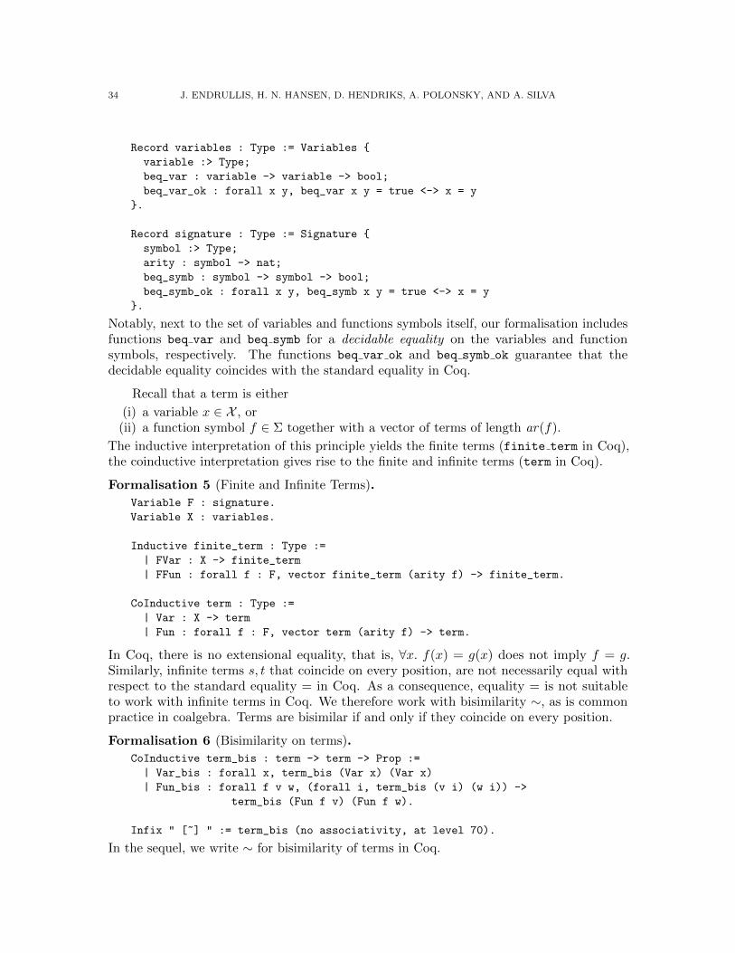
34 J. ENDRULLIS, H. N. HANSEN, D. HENDRIKS, A. POLONSKY, AND A. SILVA
Record variables : Type := Variables {
variable :> Type;
beq_var : variable -> variable -> bool;
beq_var_ok : forall x y, beq_var x y = true <-> x = y
}.
Record signature : Type := Signature {
symbol :> Type;
arity : symbol -> nat;
beq_symb : symbol -> symbol -> bool;
beq_symb_ok : forall x y, beq_symb x y = true <-> x = y
}.
Notably, next to the set of variables and functions symbols itself, our formalisation includesfunctions beq var and beq symb for a decidable equality on the variables and functionsymbols, respectively. The functions beq var ok and beq symb ok guarantee that thedecidable equality coincides with the standard equality in Coq.
Recall that a term is either
(i) a variable x ∈ X , or(ii) a function symbol f ∈ Σ together with a vector of terms of length ar(f).
The inductive interpretation of this principle yields the finite terms (finite term in Coq),the coinductive interpretation gives rise to the finite and infinite terms (term in Coq).
Formalisation 5 (Finite and Infinite Terms).
Variable F : signature.
Variable X : variables.
Inductive finite_term : Type :=
| FVar : X -> finite_term
| FFun : forall f : F, vector finite_term (arity f) -> finite_term.
CoInductive term : Type :=
| Var : X -> term
| Fun : forall f : F, vector term (arity f) -> term.
In Coq, there is no extensional equality, that is, ∀x. f(x) = g(x) does not imply f = g.Similarly, infinite terms s, t that coincide on every position, are not necessarily equal withrespect to the standard equality = in Coq. As a consequence, equality = is not suitableto work with infinite terms in Coq. We therefore work with bisimilarity ∼, as is commonpractice in coalgebra. Terms are bisimilar if and only if they coincide on every position.
Formalisation 6 (Bisimilarity on terms).
CoInductive term_bis : term -> term -> Prop :=
| Var_bis : forall x, term_bis (Var x) (Var x)
| Fun_bis : forall f v w, (forall i, term_bis (v i) (w i)) ->
term_bis (Fun f v) (Fun f w).
Infix " [~] " := term_bis (no associativity, at level 70).
In the sequel, we write ∼ for bisimilarity of terms in Coq.

COINDUCTIVE FOUNDATIONS OF INFINITARY REWRITING AND EQUATIONAL LOGIC 35
9.3. Formalisation of Term Rewriting Systems. Next, we formalise rewrite rules andterm rewriting systems as lists of rules. In the following definition, we leave is var, vars,inc and list implicit; the function
(i) is var : term → bool returns true if and only if the given term is a variable,(ii) vars : finite term → (X → Prop) returns the set of variables in a term,(iii) inc stands for set inclusion, and(iv) list is the implementation of lists in the standard library of Coq.
Formalisation 7 (Rules and term rewriting systems). These are formalized as
Record rule : Type := Rule {
lhs : finite_term;
rhs : term;
rule_wf : is_var lhs = false /\ inc (vars rhs) (vars lhs)
}.
Definition trs := list rule.
A rule consists of a finite left-hand side (lhs) and finite or infinite right-hand side (rhs),and a proposition rule wf stating that the lhs is not a variable, and the variables in rhs
are a subset of the variables in lhs.
Remark 9.1. We note that the definition of rules could easily be generalised to infiniteleft-hand sides. This is not a restriction of our coinductive framework for infinitary rewriting.In the literature, infinitary term rewriting systems are typically defined to have finite left-hand sides to keep matching (with respect to left-linear rules) decidable. We have chosen toadopt this restriction as our goal was a formalisation of the Compression Lemma which onlyholds for term rewrite systems with finite (and linear) left-hand sides.
We introduce substitutions as maps from variables to finite or infinite terms.
Formalisation 8 (Substitution).
Definition substitution := X -> term.
CoFixpoint substitute (sigma : substitution) (t : term) : term :=
match t with
| Var x => sigma x
| Fun f args => Fun f (vmap (substitute sigma) args)
end.
The substitute function applies a substitution to a finite or infinite term.
9.4. Formalisation of Infinitary Rewriting. The closure of the rules under substitutionsgives rise to root steps on finite and infinite terms.
Formalisation 9 (Root steps on finite and infinite terms).
Variable system : trs.
Inductive root_step : relation term :=
| Root_step :
forall (s t : term) (r : rule) (u : substitution),
In r system ->

36 J. ENDRULLIS, H. N. HANSEN, D. HENDRIKS, A. POLONSKY, AND A. SILVA
substitute u (lhs r) [~] s ->
substitute u (rhs r) [~] t ->
root_step s t.
As discussed above, we must include bisimilarity ∼ since the equality = in Coq is too strict.Here ‘In r system’ checks whether r (a rule) occurs in system (a list of rules).
We formalise the lifting operation R (Definition 3.1) as follows.
Formalisation 10 (Lifting).
Inductive lift (R : relation term) : relation term :=
| lift_id : forall s t, s [~] t -> lift R s t
| lift_step :
forall (f : F) (s t : vector term (arity f)),
(forall i, R (s i) (t i)) ->
forall fs ft, Fun f s [~] fs -> Fun f t [~] ft -> lift R fs ft.
Again, we include bisimilarity ∼ instead of the standard equality = in Coq.
We use the root step rewrite relation and the lifting operation to introduce infinitarystrongly convergent reductions. Our coinductive definition (Definition 4.3) is based on mixedinduction and coinduction:
→∞ := µR. νS. (→ε ∪ R)∗ ; S .
Unfortunately, Coq has no support for mutual inductive and coinductive definitions.To overcome this problem, we employ the fact that the greatest fixed point νS. F (S) is
the union of all S for which S ⊆ F (S) (under the condition that F : L→ L is monotone);see further Section 3. In other words, νS. F (S) is the smallest relation T such that S ⊆ Twhenever S ⊆ F (S). Hence, we have
→∞ := µR.
( the smallest T such that:for all relations S,S ⊆ (→ε ∪ R)∗ ; S =⇒ S ⊆ T
)(9.1)
This definition lends itself to a formalisation in Coq.
Formalisation 11. Formalisation of (9.1):
Inductive ired : relation (term F X) :=
| Ired :
forall S : relation (term F X),
subrel S ((root_step (+) lift ired)* ;; lift S) ->
subrel S ired.
Here ;; is relation composition, (+) is the union, and * the reflexive-transitive closure. Thestatement Inductive ired in the formalisation corresponds to µR in (9.1), and thus iredcorresponds to R.
While Formalisation 11 is correct, it turns out that Coq is not able to generate a goodinduction principle from the definition. The generated induction principle is:
ired_ind : forall P : term -> term -> Prop,
( forall S : relation term,
subrel S ((root_step (+) lift ired)* ;; lift S) -> subrel S P )
-> subrel ired P

COINDUCTIVE FOUNDATIONS OF INFINITARY REWRITING AND EQUATIONAL LOGIC 37
In mathematical notation this reads as follows:
∀P.(∀S.
(S ⊆ (→ε ∪ ired)∗ ; S
)→ S ⊆ P
)→ ired ⊆ P
Note that, in particular we have ired = (→ε ∪ ired)∗. As a consequence, we already haveto show ired ⊆ P as part of the induction step. Hence, this induction principle is void.
To overcome this problem, we adapt (9.1) and Formalisation 11 as follows:
→∞ := µR.
( the smallest T such that:for all relations S and I,I ⊆ R =⇒ S ⊆ (→ε ∪ I)∗ ; S =⇒ S ⊆ T
)(9.2)
To help Coq generate a good induction principle, we introduce an auxiliary relation I, andwe replace the occurrences of R in the body of the definition by I. To preserve the semanticsof the definition, we require I ⊆ ired. (In other words, I is a lower-approximant of R.)
To see that (9.1) and (9.2) give rise to the same relation →∞, we argue as follows. Ifwe were to replace I ⊆ R by I = R in (9.2), then both definitions would obviously coincide.However, both definitions also coincide without the replacement since sets I ( R do notcontribute due to monotonicity.
We formalise (9.2) as follows.
Formalisation 12 (Strongly convergent rewrite relation). 1
Inductive ired : relation term :=
| Ired :
forall S I : relation term,
subrel I ired ->
subrel S ((root_step (+) lift I)* ;; lift S) ->
subrel S ired.
Remark 9.2. For this definition, Coq generates the following good induction principle:
ired_ind : forall P : term -> term -> Prop,
( forall S I : relation (term F X),
subrel I ired ->
subrel I P ->
subrel S ((root_step (+) lift I)* ;; lift S) ->
subrel S P) ->
subrel ired P
Thus in order to prove →∞ ⊆ P , it suffices to show
I ⊂ →∞ =⇒ I ⊆ P =⇒ S ⊆ (→ε ∪ I)∗ ; S =⇒ S ⊆ Pfor every relation I and S. Below, we will see in several examples, that this is a usefulinduction principle that is easy to work with.
1Note that canonical proof trees could be formalised by a small adaptation of this formalization. On theone hand, the restricted (canonical) proof trees can simplify proofs whose source is (a proof tree for) aninfinite reduction. On the other hand, the restriction might complicate proofs whose target is (a proof treefor) an infinite reduction. To combine the advantages of both choices, it would be interesting to formallyprove that every proof tree can be transformed into an equivalent canonical proof tree.

38 J. ENDRULLIS, H. N. HANSEN, D. HENDRIKS, A. POLONSKY, AND A. SILVA
9.5. Formalisation of Omega Rewriting. In order to formalise the Compression Lemma,we need rewrite sequences of length ≤ ω. To formalise →≤ω, we use
→≤ω := νR. (→∗ ;R) (9.3)
That is, a rewrite sequence of length ≤ ω is a finite rewrite sequence followed by rewritesequences of length ≤ ω on subterms (below the root). Using dovetailing, this gives rise tothe usual concept of rewrite sequences indexed by an ordinal ≤ ω.
As above for →∞, we have:
→≤ω :=the smallest T such that:for all relations S, S ⊆ (→∗ ; S) =⇒ S ⊆ T (9.4)
This definition can be formalised in Coq as follows.
Formalisation 13 (Rewrite sequences of length at most ω).
Inductive ored : relation term :=
| Ored :
forall S : relation term,
subrel S (mred ;; lift S) ->
subrel S ored.
Here mred are finite rewrite sequences →∗.To keep the proof of compression in Coq as simple as possible, we have chosen to define
the finite rewrite relation →∗ in a non-standard way. We introduce mred as the smallestrelation S that fulfils the following conditions:
(i) mred bis: if s S t, s ∼ s′ and t ∼ t′, then s′ S t′,(ii) mred refl: S is reflexive,(iii) mred trans: S is transitive,(iv) mred root: →ε ⊆ S, and(v) mred fun: if u1 S v1, . . . , un S vn, then f(u1, . . . , un) S f(v1, . . . , vn).
Let us check that mred indeed is the finite rewrite relation →∗:(a) For mred ⊆ →∗ note that the finite rewrite relation →∗ fulfils all these criteria.(b) For →∗ ⊆ mred we argue as follows. We have →ε ⊆ mred by mred root. By mred fun
together with mred refl it follows that mred is closed under contexts. Thus → ⊆ mred.By mred refl and mred trans we obtain that →∗ ⊆ mred.
Hence mred =→∗.Formalisation 14 (Finite rewriting relation on infinite terms).
Inductive mred : relation term :=
| mred_bis :
forall s s’ t t’, s [~] s’ -> t [~] t’ -> mred s t -> mred s’ t’
| mred_refl :
forall s, mred s s
| mred_trans :
forall s t u, mred s t -> mred t u -> mred s u
| mred_root :
forall (s t : term F X) , root_step s t -> mred s t
| mred_fun :
forall (f : F) (u v : vector (term F X) (arity f)),
(forall i : Fin (arity f), mred (u i) (v i)) ->
mred (Fun f u) (Fun f v).

COINDUCTIVE FOUNDATIONS OF INFINITARY REWRITING AND EQUATIONAL LOGIC 39
Notation 9.3. In the remainder of this section, we will write
→m for mred , →i for ired , →o for ored , and →r for root step.
We have formalised Lemma 9.6 to show that Formalisation 13 of ored indeed correspondsto Equation 9.3. We first prove two auxiliary facts.
Lemma 9.4 (ored subrel). We have →o ⊆ →m ;→o.
Proof. Let s→o t. By definition of →o there exists a relation S ⊆ →o such that S ⊆ →m ;Sand s S t. As s→m ; S t and S ⊆ →o, we have s→m ;→o t.
Lemma 9.5 (subrel lift ored ored). We have →o ⊆ →o.
Proof. Let s→o t. Define S =→o ∪ 〈s, t〉. Then we have s S t. To prove s→o t, it suffices(by definition of →o) to show that S ⊆ →m ; S. By Lemma 9.4, we have →o ⊆ →m ;→o,and hence →o ⊆ →m ; S. Moreover, we have 〈s, t〉 ∈ →m ; S as a consequence of reflexivelyof →m, and since s→o t and →o ⊆ S imply s S t. This concludes the proof.
Lemma 9.6 (ored ok). We have →o =→m ;→o.
Proof. By Lemma 9.4 it suffices to show that →m ;→o ⊆ →o. Let s→m t→o u. Then, byLemma 9.5, we have s→m t→o u. By definition of →o there exists a relation S ⊆ →o suchthat S ⊆ →m ; S and t S u. Thus t →m t′ S u for some t′. Define S′ = S ∪ 〈s, u〉. Thens S′ u and S′ ⊆ →m ; S′ since s →m t′ S′ u by mred trans and S ⊆ S′. Hence s →o u bydefinition of →o using S′.
9.6. Formalisation of the Compression Lemma. Using the above definitions, we willnow prove the Compression Lemma. The proof realises a transformation of →∞ proof treesinto →≤ω proof trees.
Lemma 9.7 (Compression Lemma). Let R be a left-linear term rewriting system with finiteleft-hand sides. Whenever there is an infinite reduction from s to t (s →∞ t) then thereexists a reduction of length at most ω from s to t (s→≤ω t).
We have formalised the Compression Lemma as follows:
Lemma 9.8. For left-linear trs’s we have →i ⊆ →o.
The condition finite left-hand sides is part of the formalisation of trs’s, see above. In theremainder of this section we tacitly assume that the underlying trs is left-linear. This is anecessary condition for all lemmas 9.9–9.15.
We present the proof of Lemma 9.8 as close as possible to to our formalisation in Coq.We begin with a few auxiliary lemmas.
Lemma 9.9 (ored match). If s→o `σ for a finite, linear term `, then s→m `τ for somesubstitution τ with ∀x. τ(x)→o σ(x).
Proof. The proof proceeds by induction on `. If s →o `σ, then there exists a term t suchthat s →m t →o `σ. Assume that ` is a variable, say ` = x. Then define τ(x) = t andτ(y) = σ(y) for every y 6= x. We have τ(x) = t→o `σ = σ(x). Then s→m `τ , and we have∀x. τ(x)→o σ(x) since →o ⊆ →o by Lemma 9.5 and →o is reflexive.
If ` is not a variable, let ` = f(`1, . . . , `n). Then t→o `σ implies that t = f(t1, . . . , tn)for some terms t1, . . . , tn, and we have ti →o `iσ for every i ∈ {1, . . . , n}. Then by induction

40 J. ENDRULLIS, H. N. HANSEN, D. HENDRIKS, A. POLONSKY, AND A. SILVA
hypothesis, we have ti →m `iτi and ∀x. τi(x)→o σ(x) for every i ∈ {1, . . . , n}. From linearityof ` it follows that `1, . . . , `n do not share any variables. Consequently, we can define thesubstitution τ as follows: τ(x) = τi(x) if x ∈ Var(`i) and τ(x) = σ(x) if x 6∈ Var(`).Then `iτ = `iτi for every i ∈ {1, . . . , n} and `τ = f(`1τ1, . . . , `nτn). Moreover we have∀x. τ(x)→o σ(x) by definition of τ . It remains to show s→m `τ . Using mred fun we gett = f(t1, . . . , tn)→m f(`1τ1, . . . , `nτn) = `τ . By mred trans we obtain s→m `τ .
Lemma 9.10 (subsitution ored). Let t be a (finite or infinite) term and σ, τ substitutionssuch that σ(x)→o τ(x) for every x ∈ Var(t). Then tσ →o tτ .
Proof. By definition of →o it suffices to find a relation S such that tσ S tτ and S ⊆ →m ; S.We define S =→o ∪ { 〈uσ, uτ〉 | u a term }. We show S ⊆ →m ; S. We have
→o ⊆ →m ;→o ⊆ →m ; S (9.5)
by Lemma 9.6.So consider uσ S uτ for some term u. If u is a variable, then uσ = σ(u)→o τ(u) = uτ .
Then uσ →m ; S uτ follows from (9.5). Thus, let u = f(u1, . . . , un) for some symbol f andterms u1, . . . , un. Then we have uσ = f(u1σ, . . . , unσ) S f(u1τ, . . . , unτ) = uτ , and clearlyS ⊆ →m ; S. Hence S ⊆ →m ; S.
Lemma 9.11 (ored rstep). We have →o ;→r ⊆ →o.
Proof. Let ` → r ∈ R be a rule, σ a substitution and consider s →o `σ →r rσ. Then byLemma 9.9 we have s →m `τ for some substitution τ with ∀x. τ(x) →o σ(x). We haverτ →o rσ by Lemma 9.10, and thus rτ →m t→o rσ for some t by Lemma 9.6. Then alsos→m `τ →r rτ →m t→o rσ and s→m t→o rσ by mred root and mred trans. Hence wehave s→o rσ by Lemma 9.6.
Lemma 9.12 (ored mred). We have →o ;→m ⊆ →o.
Proof. The proof proceeds by induction on the definition of →m in s →o t →m u. Theinduction step is trivial for mred bis, mred refl and mred trans. For mred root the claimfollows from Lemma 9.11. Here we only consider the case of mred fun. Then t = f(t1, . . . , tn)and u = f(u1, . . . , un) for some symbol f and ti →m ui for every i ∈ {1, . . . , n}. Froms →o t it follows that s →m s′ →o t = f(t1, . . . , tn) for some s′. Hence s′ = f(s1, . . . , sn)with si →o ti for every i ∈ {1, . . . , n}. By the induction hypothesis, we obtain si →o ui forevery i ∈ {1, . . . , n}, and, consequently, s→m s′ →o u. Finally, s→o u by Lemma 9.6.
Lemma 9.13 (ored ored). We have →o ;→o ⊆ →o and →o ;→o ⊆ →o.
Proof. Define S = (→o ;→o)∪ (→o ;→o). We show S ⊆ →o. By definition of →o it sufficesthat S ⊆ →m ; S. We have:
→o ;→o ⊆ →o ; (→m ;→o) ⊆ →o ;→o (9.6)
by Lemma 9.6 and Lemma 9.12, and
→o ;→o ⊆ (→m ;→o) ;→o ⊆ →m ; (→o ;→o) ⊆ →m ; (→o ;→o) ⊆ →m ; S
by Lemma 9.6, associativity, definition of · . This proves S ⊆ →m ; S.

COINDUCTIVE FOUNDATIONS OF INFINITARY REWRITING AND EQUATIONAL LOGIC 41
Lemma 9.14 (ored mix). We have (→r ∪→o )∗ ⊆ →o.
Proof. Define S = (→r ∪→o ). We prove S∗ ⊆ →o by induction on (the definition of) thereflexive transitive closure:
(i) refl trans step: For s S t we have either s →r t or s →o t. Then s →o t as aconsequence of either Lemma 9.11 or Lemma 9.6, respectively.
(ii) refl trans refl: For s ∼ t we s →m t by mred bis and mred refl. Hence s →o tsince →m ;→o ⊆→o by Lemma 9.6 and →o is reflexive by lift id.
(iii) refl trans trans: For s S∗ u S∗ t we obtain s →o u and u →o t by inductionhypothesis. Then s→o t follows from Lemma 9.13.
Lemma 9.15 (ored liftR). We have R ⊆ →o ; R implies R ⊆ →o.
Proof. Define S = (→o ; R) ∪ (→o ; R). We show S ⊆ (→m ; S):
→o ; R ⊆ →o ; (→o ; R) ⊆ →o ; R
by R ⊆ →o ; R and Lemma 9.13, and
→o ; R ⊆ (→m ;→o) ; R ⊆ →m ; (→o ; R) ⊆ →m ; S
by Lemma 9.6. Hence S ⊆ (→m ; S) and consequently S ⊆ →o. Note that R ⊆ →o ; R ⊆ S.Thus R ⊆ S ⊆ →o.
We are ready to prove compression.
Proof of Lemma 9.8. The proof proceeds by induction on →i. By the induction principlediscussed in Remark 9.2 we have to show
I ⊂ →i =⇒ I ⊆ →o =⇒ S ⊆ (→r ∪ I)∗ ; S =⇒ S ⊆ →o
for every relation I and S. So let I ⊆ (→i ∩→o) and S ⊆ (→r ∪ I)∗ ; S. Since I ⊆ →o weget (→r ∪ I)∗ ⊆ (→r ∪ →o)
∗ ⊆ →o by Lemma 9.14. Consequently, S ⊆ →o ; S and, byLemma 9.15, we obtain S ⊆ →o. Hence →i ⊆ →o.
To the best of our knowledge this is the first formal proof of this well-known lemma.The formalization is available at [17].
10. Conclusion
We have proposed a coinductive framework which gives rise to several natural variants ofinfinitary rewriting in a uniform way:
(a) infinitary equational reasoning∞= := νy. (←ε ∪ →ε ∪ y)∗,
(b) bi-infinite rewriting∞→ := νy. (→ε ∪ y)∗, and
(c) infinitary rewriting →∞ := µx. νy. (→ε ∪ x)∗ ; y .
We believe that (a) and (b) are novel. As a consequence of the coinduction over the termstructure, these notions have the strong convergence built-in, and thus can profit from thewell-developed techniques (such as tracing) in infinitary rewriting.
We have given a mixed inductive/coinductive definition of infinitary rewriting andestablished a bridge between infinitary rewriting and coalgebra. Both fields are concernedwith infinite objects and we would like to understand their relation better. In contrast toprevious coinductive treatments, the framework presented here captures rewrite sequences of

42 J. ENDRULLIS, H. N. HANSEN, D. HENDRIKS, A. POLONSKY, AND A. SILVA
arbitrary ordinal length, and paves the way for formalizing infinitary rewriting in theoremprovers (as illustrated by our proof of the Compression Lemma in Coq).
Concerning proof trees/terms for infinite reductions, let us mention that an alternativeapproach has been developed in parallel by Lombardi, Rıos and de Vrijer [32]. While wefocus on proof terms for the reduction relation and abstract from the order of steps in parallelsubterms, they use proof terms for modeling the fine-structure of the infinite reductionsthemselves. Another difference is that our framework allows for non-left-linear systems. Webelieve that both approaches are complementary. Theorems for which the fine-structure ofrewrite sequences is crucial, must be handled using [32]. (But note that we can capturestandard reductions by a restriction on proof trees and prove standardization using prooftree transformations, see [22]). If the fine-structure is not important, as for instance forproving confluence, then our system is more convenient to work with due to simpler proofterms.
Our work lays the foundation for several directions of future research:
(i) The coinductive treatment of infinitary λ-calculus [22] has led to elegant, significantlysimpler proofs [10, 11] of some central properties of the infinitary λ-calculus. Thecoinductive framework that we propose enables similar developments for infinitaryterm rewriting with reductions of arbitrary ordinal length.
(ii) The concepts of bi-infinite rewriting is novel, and the theory of infinitary equationalreasoning is still underdeveloped. It would be interesting to study these concepts.Is there an equivalent of ordinal-indexed rewrite sequences for bi-infinite rewriting(maybe using Conway’s surreal numbers [7])? Is it possible to establish some sort ofCompression Lemma for bi-infinite rewriting?
Moreover, it would be fruitful to compare the Church–Rosser properties∞= ⊆ →∞ ; →∞ and ( →∞ ;→∞)∗ ⊆ →∞ ; →∞ .
(iii) The formalization of the proof of the Compression Lemma in Coq is just the first steptowards the formalization of all major theorems in infinitary rewriting.
It would also be interesting to formalise infinitary equational reasoning∞= and
bi-infinite rewriting∞→ in Coq. We expect that it is straightforward to adapt our Coq
formalization of infinitary rewriting →∞ to equational reasoning∞= and bi-infinite
rewriting∞→. The latter two concepts have significantly simpler definitions in the fixed
point calculus.(iv) It is interesting to investigate how the coinductive framework should be extended to
incorporate the infinitary analysis of meaningless terms. [3, 2, 4, 21] This would bethe natural stepping-stone to the formalization of confluence theorems in infinitaryrewriting extended with ⊥-reduction.
(v) We believe that the coinductive definitions will ease the development of new techniquesfor automated reasoning about infinitary rewriting. For example, methods for proving(local) productivity [14, 18, 38], for (local) infinitary normalization [37, 15, 13], for(local) unique normal forms [20], and for analysis of infinitary reachability and infinitaryconfluence. Due to the coinductive definitions, the implementation and formalizationof these techniques could make use of circular coinduction [23, 19].

COINDUCTIVE FOUNDATIONS OF INFINITARY REWRITING AND EQUATIONAL LOGIC 43
Acknowledgments. We thank Patrick Bahr, Jeroen Ketema, and Vincent van Oostromfor fruitful discussions and comments on earlier versions of this paper. We are thankful tothe reviewers for pointing out mistakes and suggesting several improvements.
References
[1] F. Baader and T. Nipkow. Term Rewriting and All That. Cambridge Univ. Press, 1998.[2] P. Bahr. Abstract Models of Transfinite Reductions. In Proc. Conf. on Rewriting Techniques and
Applications (RTA 2010), volume 6 of Leibniz International Proceedings in Informatics, pages 49–66.Schloss Dagstuhl, 2010.
[3] P. Bahr. Partial Order Infinitary Term Rewriting and Bohm Trees. In Proc. Conf. on Rewriting Techniquesand Applications (RTA 2010), volume 6 of Leibniz International Proceedings in Informatics, pages 67–84.Schloss Dagstuhl, 2010.
[4] P. Bahr. Infinitary Term Graph Rewriting is Simple, Sound and Complete. In Proc. Conf. on RewritingTechniques and Applications (RTA 2012), volume 15 of Leibniz International Proceedings in Informatics,pages 69–84. Schloss Dagstuhl, 2012.
[5] H.P. Barendregt. The Type Free Lambda Calculus. In Handbook of Mathematical Logic, pages 1091–1132.Nort-Holland Publishing Company, Amsterdam, 1977.
[6] H.P. Barendregt and J.W. Klop. Applications of Infinitary Lambda Calculus. Information and Computa-tion, 207(5):559–582, 2009.
[7] J.H. Conway. On Numbers and Games. Ak Peters Series. Taylor & Francis, 2000.[8] C. Coquand and Th. Coquand. On the Definition of Reduction for Infinite Terms. Comptes Rendus de
l’Academie des Sciences. Serie I, 323(5):553–558, 1996.[9] Th. Coquand. Infinite objects in type theory. In Henk Barendregt and Tobias Nipkow, editors, Types
for Proofs and Programs, International Workshop TYPES’93, Nijmegen, The Netherlands, May 24–28,1993, Selected Papers, volume 806 of LNCS, pages 62–78. Springer, 1994.
[10] L. Czajka. A Coinductive Confluence Proof for Infinitary Lambda-Calculus. In Rewriting and TypedLambda Calculi (RTA-TLCA 2014), volume 8560 of Lecture Notes in Computer Science, pages 164–178.Springer, 2014.
[11] L. Czajka. Coinductive Techniques in Infinitary Lambda-Calculus. ArXiv e-prints, 2015.[12] N. Dershowitz, S. Kaplan, and D.A. Plaisted. Rewrite, Rewrite, Rewrite, Rewrite, Rewrite,. . . . Theoretical
Computer Science, 83(1):71–96, 1991.[13] J. Endrullis, R. C. de Vrijer, and J. Waldmann. Local Termination: Theory and Practice. Logical Methods
in Computer Science, 6(3), 2010.[14] J. Endrullis, C. Grabmayer, and D. Hendriks. Complexity of Fractran and Productivity. In Proc. Conf.
on Automated Deduction (CADE 22), volume 5663 of LNCS, pages 371–387, 2009.[15] J. Endrullis, C. Grabmayer, D. Hendriks, J.W. Klop, and R.C de Vrijer. Proving Infinitary Normalization.
In Postproc. Int. Workshop on Types for Proofs and Programs (TYPES 2008), volume 5497 of LNCS,pages 64–82. Springer, 2009.
[16] J. Endrullis, H. H. Hansen, D. Hendriks, A. Polonsky, and A. Silva. A Coinductive Framework forInfinitary Rewriting and Equational Reasoning. In Proc. Conf. on Rewriting Techniques and Applications(RTA 2015), Leibniz International Proceedings in Informatics. Schloss Dagstuhl, 2015.
[17] J. Endrullis, H. H. Hansen, D. Hendriks, A. Polonsky, and A. Silva. A Formalization of the CompressionLemma, 2016. Available at http://joerg.endrullis.de/coq/compression.
[18] J. Endrullis and D. Hendriks. Lazy Productivity via Termination. Theoretical Computer Science,412(28):3203–3225, 2011.
[19] J. Endrullis, D. Hendriks, and M. Bodin. Circular Coinduction in Coq Using Bisimulation-Up-ToTechniques. In Proc. Conf. on Interactive Theorem Proving (ITP), volume 7998 of LNCS, pages 354–369.Springer, 2013.
[20] J. Endrullis, D. Hendriks, C. Grabmayer, J.W. Klop, and V. van Oostrom. Infinitary term rewritingfor weakly orthogonal systems: Properties and counterexamples. Logical Methods in Computer Science,10(2:7):1–33, 2014.
[21] J. Endrullis, D. Hendriks, and J.W. Klop. Highlights in Infinitary Rewriting and Lambda Calculus.Theoretical Computer Science, 464:48–71, 2012.

44 J. ENDRULLIS, H. N. HANSEN, D. HENDRIKS, A. POLONSKY, AND A. SILVA
[22] J. Endrullis and A. Polonsky. Infinitary Rewriting Coinductively. In Proc. Types for Proofs and Programs(TYPES 2012), volume 19 of Leibniz International Proceedings in Informatics, pages 16–27. SchlossDagstuhl, 2013.
[23] J. Goguen, K. Lin, and G. Rosu. Circular Coinductive Rewriting. In Proc. of Automated SoftwareEngineering, pages 123–131. IEEE, 2000.
[24] B. Jacobs and J.J.M.M. Rutten. An Introduction to (Co)Algebras and (Co)Induction. In AdvancedTopics in Bisimulation and Coinduction, pages 38–99. Cambridge University Press, 2011.
[25] F. Joachimski. Confluence of the Coinductive Lambda Calculus. Theoretical Computer Science, 311(1-3):105–119, 2004.
[26] S. Kahrs. Infinitary Rewriting: Closure Operators, Equivalences and Models. Acta Informatica, 50(2):123–156, 2013.
[27] J.R. Kennaway and F.-J. de Vries. Infinitary Rewriting, chapter 12. Cambridge University Press, 2003.in [35].
[28] J.R. Kennaway, J.W. Klop, M.R. Sleep, and F.-J. de Vries. Transfinite Reductions in Orthogonal TermRewriting Systems. Information and Computation, 119(1):18–38, 1995.
[29] J. Ketema and J.G. Simonsen. Computing with Infinite Terms and Infinite Reductions. Unpublishedmanuscript.
[30] J.W. Klop. Term Rewriting Systems. In Handbook of Logic in Computer Science, volume II, pages 1–116.Oxford University Press, 1992.
[31] J.W. Klop and R.C de Vrijer. Infinitary Normalization. In We Will Show Them: Essays in Honour ofDov Gabbay (2), pages 169–192. College Publications, 2005.
[32] C. Lombardi, A. Rıos, and R.C de Vrijer. Proof Terms for Infinitary Rewriting. In Rewriting and TypedLambda Calculi (RTA-TLCA 2014), volume 8560 of Lecture Notes in Computer Science, pages 303–318.Springer, 2014.
[33] S. Milius. Completely iterative algebras and completely iterative monads. ic, 196:1–41, 2005.[34] J.G. Simonsen. On Confluence and Residuals in Cauchy Convergent Transfinite Rewriting. Information
Processing Letters, 91(3):141–146, 2004.[35] Terese. Term Rewriting Systems, volume 55 of Cambridge Tracts in Theoretical Computer Science.
Cambridge University Press, 2003.[36] M. Vermaat. Infinitary Rewriting in Coq. Available at url http://martijn.vermaat.name/
master-project/.[37] H. Zantema. Normalization of Infinite Terms. In Proc. Conf. on Rewriting Techniques and Applications
(RTA 2008), number 5117 in LNCS, pages 441–455, 2008.[38] H. Zantema and M. Raffelsieper. Proving Productivity in Infinite Data Structures. In Proc. Conf. on
Rewriting Techniques and Applications (RTA 2010), volume 6 of Leibniz International Proceedings inInformatics, pages 401–416. Schloss Dagstuhl, 2010.
This work is licensed under the Creative Commons Attribution-NoDerivs License. To viewa copy of this license, visit http://creativecommons.org/licenses/by-nd/4.0/ or send aletter to Creative Commons, PO Box 1866, Mountain View, CA 9404, USA