coiling instability in liquid and solid ropes

HAL Id: tel-00156591https://tel.archives-ouvertes.fr/tel-00156591

Submitted on 21 Jun 2007

HAL is a multi-disciplinary open accessarchive for the deposit and dissemination of sci-entific research documents, whether they are pub-lished or not. The documents may come fromteaching and research institutions in France orabroad, or from public or private research centers.

L’archive ouverte pluridisciplinaire HAL, estdestinée au dépôt et à la diffusion de documentsscientifiques de niveau recherche, publiés ou non,émanant des établissements d’enseignement et derecherche français ou étrangers, des laboratoirespublics ou privés.

Coiling Instability in Liquid and Solid RopesMehdi Habibi

To cite this version:Mehdi Habibi. Coiling Instability in Liquid and Solid Ropes. Fluid Dynamics [physics.flu-dyn].Université Pierre et Marie Curie - Paris VI, 2007. English. tel-00156591

https://tel.archives-ouvertes.fr/tel-00156591

https://hal.archives-ouvertes.fr

Département de Physiquede l'É ole Normale SupérieureLaboratoire de Physique StatistiqueTHÈSE DE DOCTORATDE L'UNIVERSITÉ PARIS 6 PIERRE ET MARIE CURIESpé ialité : Physique des Liquidesprésentée parMehdi HABIBIpour obtenir le grade deDOCTEUR DE L'UNIVERSITÉ PARIS 6Sujet de la thèse :L'instabilité de Flambage Héli oïdal de Filaments Liquides et Solides( Coiling Instability in Liquid and Solid Ropes )Soutenue le 8 juin 2007 devant le jury omposé de :H. KELLAY RapporteurJ. R. LISTER RapporteurB. AUDOLY ExaminateurM. BEN AMAR ExaminateurM. R. H. KHAJEPOUR ExaminateurN. RIBE InvitéR. GOLESTANIAN Dire teur de thèseD. BONN Dire teur de thèse

Coiling Instability in Liquid and Solid Ropes

Advisors: Daniel Bonn & Ramin Golestanian

May 21, 2007

Acknowledgements

I would like to thank my supervisors, Daniel Bonn and Ramin Golestanian, from

whom I have learned a lot. I have enjoyed a professional and insightful supervision

by both of them, either directly or from the long distance. I am deeply indebted to

them for their constant support, encouragement and helping through my research.

I also thank my advisor, Mohamad Reza Khajepour, who helped me a lot at

IASBS.

I have benefitted from most fruitful collaborations on these problems with Neil

Ribe and I wish to express my gratitude to him.

I am grateful to my colleagues, Maniya Maleki at IASBS and Peder Moller at

Ecole Normale Superieure with whom I collaborated in doing the experiments in the

laboratory, as well as having good time with them as very good friends.

I have also enjoyed helpful discussions with Jacques Meunier, Jens Eggers, Mokhtar

Adda Bedia, Sebastien Moulinet, Dirk Aarts and Hamid Reza Khalesifard.

I wish to thank the hospitality of Ecole Normale Superieure in Paris and IASBS

in Zanjan.

I would like to specially thank Bahman Farnudi, who was very kind and helped

me, whenever I needed help. I also thank Nader S. Reyhani, Jafar M. Amjad, S.

Rasuli and other people who help me for the experiments at IASBS.

I am grateful to Jens Eggers and the people of School of Mathematics at Bristol

university, especially for their kind hospitality.

My visits to Paris were supported financially by the French embassy in Tehran,

IASBS and LPS.

The Institute for Advanced Studies in Basic Sciences (IASBS) has served as a

i

ii

wonderful place for scientific work as well as for an enjoyable life, throughout the

course of my graduate studies. I wish to thank Y. Sobouti , the director, M.R.H.

Kajehpour, the deputy, professors, students, and staff of the Institute, who created

such an atmosphere with their coherent cooperations.

I had wonderful time with my friends during my studies at IASBS, namely Jaber

Dehghani, Majid Abedi, Ehsan Jafari, Reza Vafabakhsh, Said Ansari, Alireza Akbari,

Roohola Jafari, Davood Noroozi, Mohamad Charsooghi, Farshid Mohamadrafie and

Sharareh Tavaddod and Didi Derks, Geoffroy Guena, Ulysse Delabre and Cristophe

Chevalier at Ecole Normale Superieure, I wish to express my sincere gratitude to all

of them.

Lastly, my special thanks go to: my family, who have always supported me during

my life; Marzie my best friend, who has always been encouraging and helpful to me.

Preface

This thesis is a joint thesis work ( these en co-tutelle) between the ENS Paris and

the IASBS Zanjan.

Since fluid mechanics is a very large field with many applications, we set up a fluid

dynamics laboratory at IASBS for doing experiments on wetting and viscous fluids.

Daniel Bonn from the Ecole Normale Superieure in Paris helped us a lot to set up

this laboratory. The experiments which are presented in this work were done at the

Laboratoire de Physique Statistique (L.P.S) of Ecole Normale Superieure, and in the

new fluid dynamics laboratory at IASBS.

This thesis is the result of a collaborative work which is evident also from the

publications shown in the publication list at the end of the thesis. The Author

collaborated with Maniya Maleki on the experiments related to Figs. 2.5 and 2.6 in

chapter 2 and with Peder Moller on the experiments and the mathematical model of

chapter 4. All the other experiments and data analysis were performed by the author.

The numerical calculations and calculations of coiling frequency were performed by

Neil Ribe; those in chapter 2, Figs. 2.8 and 2.9 and chapter 3, Fig. 3.3 were performed

by the author using Ribe’s code.

iii

Contents

Acknowledgements i

Preface iii

1 Introduction 1

1.1 Introduction . . . . . . . . . . . . . . . . . . . . . . . . . . . . . . . . 1

1.2 Previous Works . . . . . . . . . . . . . . . . . . . . . . . . . . . . . . 2

1.2.1 Fluid Buckling . . . . . . . . . . . . . . . . . . . . . . . . . . 3

1.2.2 Liquid Folding . . . . . . . . . . . . . . . . . . . . . . . . . . . 4

1.2.3 Liquid Coiling . . . . . . . . . . . . . . . . . . . . . . . . . . . 4

1.2.4 Elastic Rope Coiling . . . . . . . . . . . . . . . . . . . . . . . 5

1.3 Scope of This Thesis . . . . . . . . . . . . . . . . . . . . . . . . . . . 5

2 Liquid Rope Coiling 8

2.1 Introduction . . . . . . . . . . . . . . . . . . . . . . . . . . . . . . . . 8

2.2 Experimental System and Techniques . . . . . . . . . . . . . . . . . 8

2.3 Regimes of Coiling . . . . . . . . . . . . . . . . . . . . . . . . . . . . 11

2.4 Frequency versus height . . . . . . . . . . . . . . . . . . . . . . . . . 17

2.4.1 Viscous-Gravitational Transition . . . . . . . . . . . . . . . . 17

2.4.2 Gravitational-Inertial Transition . . . . . . . . . . . . . . . . . 18

2.5 Prediction of the Coiling Frequency of Honey at the Breakfast Table . 22

2.6 Radius of the Coil and the Rope . . . . . . . . . . . . . . . . . . . . . 22

2.6.1 Radius of the Coil . . . . . . . . . . . . . . . . . . . . . . . . 23

2.6.2 Diameter of the rope . . . . . . . . . . . . . . . . . . . . . . . 25

iv

CONTENTS v

2.7 Secondary Buckling . . . . . . . . . . . . . . . . . . . . . . . . . . . . 25

2.8 Conclusion . . . . . . . . . . . . . . . . . . . . . . . . . . . . . . . . . 29

3 Multivalued inertio-gravitational regime 30

3.1 Introduction . . . . . . . . . . . . . . . . . . . . . . . . . . . . . . . . 30

3.2 Experimental Methods . . . . . . . . . . . . . . . . . . . . . . . . . . 31

3.3 Inertio-Gravitational Coiling . . . . . . . . . . . . . . . . . . . . . . 32

3.3.1 Experimental Observations . . . . . . . . . . . . . . . . . . . 33

3.3.2 Time dependence of IG coiling and transition between states . 34

3.4 Whirling Liquid String Model . . . . . . . . . . . . . . . . . . . . . . 37

3.5 Comparison with experiment . . . . . . . . . . . . . . . . . . . . . . . 41

3.6 Resonant Oscillation of the Tail in Mutivalued Regime . . . . . . . . 41

3.7 Stability of Liquid Rope Coiling . . . . . . . . . . . . . . . . . . . . . 44

3.8 Conclusion . . . . . . . . . . . . . . . . . . . . . . . . . . . . . . . . . 48

4 Spiral Bubble Pattern in Liquid Rope Coiling 50

4.1 Introduction . . . . . . . . . . . . . . . . . . . . . . . . . . . . . . . . 50

4.2 Experimental Process . . . . . . . . . . . . . . . . . . . . . . . . . . . 53

4.3 The Regime of Spiral Bubble Patterns . . . . . . . . . . . . . . . . . 55

4.4 A Simple Model For The Spiral Pattern Formation . . . . . . . . . . 57

4.5 Conclusion . . . . . . . . . . . . . . . . . . . . . . . . . . . . . . . . . 62

5 Rope Coiling 63

5.1 Introduction . . . . . . . . . . . . . . . . . . . . . . . . . . . . . . . . 63

5.2 Experimental Methods . . . . . . . . . . . . . . . . . . . . . . . . . . 65

5.3 Young’s Modulus Measurements . . . . . . . . . . . . . . . . . . . . 66

5.4 Experimental Observations . . . . . . . . . . . . . . . . . . . . . . . . 68

5.5 Numerical Slender-rope Model . . . . . . . . . . . . . . . . . . . . . 70

5.6 Comparison With Experiment and With Liquid Rope Coiling . . . . 74

5.7 Conclusions . . . . . . . . . . . . . . . . . . . . . . . . . . . . . . . . 76

6 General Conclusion 78

CONTENTS vi

A Numerical Model 83

A.1 Introduction: . . . . . . . . . . . . . . . . . . . . . . . . . . . . . . . 83

A.2 Numerical model for liquid coiling and the homotopy method to solve

the equations: . . . . . . . . . . . . . . . . . . . . . . . . . . . . . . . 83

A.3 Linear stability analysis for instability of liquid coiling in multi-valued

regime : . . . . . . . . . . . . . . . . . . . . . . . . . . . . . . . . . . 89

Bibliography 91

List of Publications 96

List of Figures

1.1 A viscous jet of silicon oil falling onto a plate. . . . . . . . . . . . . . 2

1.2 Coiling of elastic rope on solid surface. . . . . . . . . . . . . . . . . . 2

1.3 Periodic folding of a sheet of glucose syrup. . . . . . . . . . . . . . . . 4

2.1 Coiling of a jet of viscous corn syrup. . . . . . . . . . . . . . . . . . . 10

2.2 Experimental setups. . . . . . . . . . . . . . . . . . . . . . . . . . . 12

2.3 Dimensionless coiling frequency. . . . . . . . . . . . . . . . . . . . . . 14

2.4 Different coiling regimes. . . . . . . . . . . . . . . . . . . . . . . . . . 15

2.5 Rope of silicon oil. . . . . . . . . . . . . . . . . . . . . . . . . . . . . 16

2.6 Curves of angular coiling frequency vs fall height. . . . . . . . . . . . 19

2.7 Transition from viscous to gravitational coiling. . . . . . . . . . . . . 21

2.8 Examples of liquid rope coiling. . . . . . . . . . . . . . . . . . . . . . 23

2.9 Coil diameter 2R as a function of height. . . . . . . . . . . . . . . . . 24

2.10 Rope radius a1 within the coil as a function of height. . . . . . . . . . 26

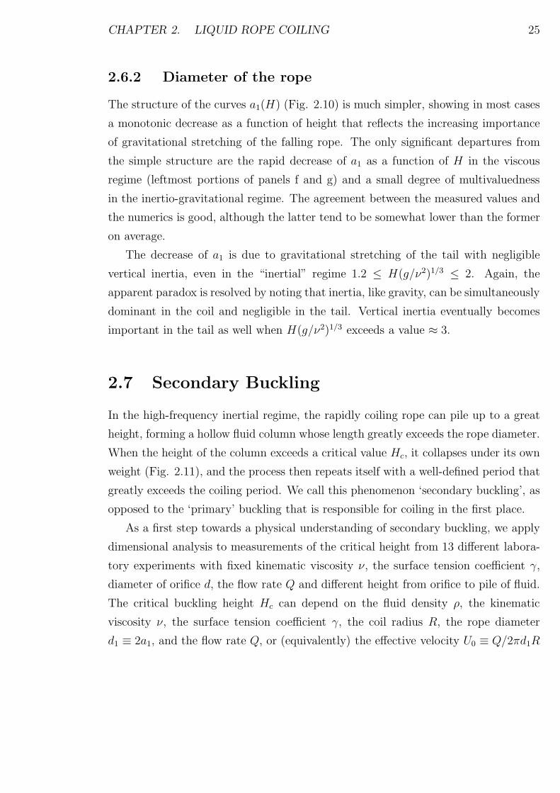
2.11 Secondary buckling of the coil in the inertial regime. . . . . . . . . . . 27

2.12 Critical height for secondary buckling as a function of the dimensionless

parameters. . . . . . . . . . . . . . . . . . . . . . . . . . . . . . . . . 28

3.1 Regimes of liquid rope coiling. . . . . . . . . . . . . . . . . . . . . . . 32

3.2 Coexisting coiling states. . . . . . . . . . . . . . . . . . . . . . . . . . 34

3.3 Rescaled coiling frequency as a function of the rescaled fall height. . . 35

3.4 Intermediate ‘figure of eight’ state. . . . . . . . . . . . . . . . . . . . 36

3.5 Coiling frequency as a function of time. . . . . . . . . . . . . . . . . . 37

vii

LIST OF FIGURES viii

3.6 Geometry of liquid rope. . . . . . . . . . . . . . . . . . . . . . . . . . 39

3.7 First six eigenfrequencies Ωn(k) of the boundary-value problem. . . . 40

3.8 Ω/ΩIG vs. ΩG/ΩIG in the limit of strong stretching. . . . . . . . . . . 42

3.9 Comparison of experimentally measured and numerically predicted fre-

quencies. . . . . . . . . . . . . . . . . . . . . . . . . . . . . . . . . . . 43

3.10 Stability of steady coiling. . . . . . . . . . . . . . . . . . . . . . . . . 45

3.11 Same as Fig. 3.10, but for Π1 = 3690, Π2 = 2.19, and Π3 = 0.044. . . 46

3.12 Same as Fig. 3.10, but for Π1 = 10050, Π2 = 3.18, and Π3 = 0.048. . . 47

4.1 Liquid rope coiling. . . . . . . . . . . . . . . . . . . . . . . . . . . . . 52

4.2 Inside a quite narrow region of the control parameter space, the coiling

rope traps bubbles of air. . . . . . . . . . . . . . . . . . . . . . . . . . 54

4.3 The process of air trapping and bubble formation. . . . . . . . . . . . 54

4.4 Numerically predicted curve of angular coiling frequency vs fall height. 56

4.5 In rare instances the liquid rope spontaneously changes the direction

of coiling. . . . . . . . . . . . . . . . . . . . . . . . . . . . . . . . . . 56

4.6 Different shapes of the branches . . . . . . . . . . . . . . . . . . . . . 57

4.7 Coiling around a center which moves on a circle of its own. . . . . . . 58

4.8 A model of the path laid down by the coil. . . . . . . . . . . . . . . 60

4.9 Patterns of bubbles generated at positions 1, 2, 3, 4, and 5 in Fig. 4.8. 60

4.10 A fit of the theoretical model for the bubble patterns to the experi-

mental data. . . . . . . . . . . . . . . . . . . . . . . . . . . . . . . . . 61

5.1 The first setup for rope experiment. . . . . . . . . . . . . . . . . . . . 67

5.2 Deflection of Spaghetti. . . . . . . . . . . . . . . . . . . . . . . . . . . 68

5.3 Deflection vs. length for spaghetti N7 . . . . . . . . . . . . . . . . . 69

5.4 Typical coiling configurations for some of the ropes. . . . . . . . . . . 70

5.5 Selected experimental measurements of the coil radius R. . . . . . . . 71

5.6 Dimensionless coiling frequency Ω ≡ Ω(d2E/ρg4)1/6 as a function of

dimensionless fall height. . . . . . . . . . . . . . . . . . . . . . . . . . 75

5.7 Comparison of experimentally measured and numerically calculated

coiling frequencies. . . . . . . . . . . . . . . . . . . . . . . . . . . . . 77

LIST OF FIGURES ix

A.1 Geometry of a viscous jet. . . . . . . . . . . . . . . . . . . . . . . . . 84

Chapter 1

Introduction

1.1 Introduction

A thin stream of honey poured from a sufficient height onto toast forms a regular

coil. A similar phenomenon happens for a falling viscous sheet: it folds. Why does

this happen, and what determines the frequency of coiling or folding? When pouring

a viscous liquid on a solid surface, we encounter instabilities. A high viscosity can

allow instabilities like buckling which normally happens only for solids, to happen

for a liquid. In solid mechanics, the concept of buckling is an important and well-

understood phenomenon. Buckling, which means the transition from a straight to a

bent configuration due to the application a load, occurs because the straight configu-

ration is not stable. This instability arises as a result of the competition between axial

compression and bending in slender objects [1]. Within the realm of fluid mechanics,

similar phenomena can be observed. An example is coiling of a thin stream of honey

as it falls onto a flat plate. The spontaneous transition from a steady, stable flow

to oscillations of parts of the jet column is called fluid buckling, in analogy with its

counterpart in solid mechanics (Fig. 1.1).

When a vertical thin flexible rope falls on a horizontal surface such as a floor a

similar phenomenon to liquid coiling is observed. This familiar phenomenon can also

be reproduced at the lunch table when a spaghetti falls down into one’s plate, (Fig.

1.2). When the rope reaches the surface it buckles and then starts to coil regularly.

1

CHAPTER 1. INTRODUCTION 2

Figure 1.1: A viscous jet of silicon oil falling onto a plate. a) stable, unbuckled jet,b) buckled jet at critical height, c) coiling jet. The scale shown is 1 mm.

Figure 1.2: Coiling of elastic rope on solid surface. a) Spaghetti b) Cotton rope.

If the rope is fed continuously towards the surface from a fixed height its motion

quickly settles down into a steady state in which the rope is laid out in a circular coil

of uniform radius. The radius of the coil which depends on the height, stiffness and

feeding velocity, determines the frequency of coiling.

1.2 Previous Works

The coiling instability of liquid filaments was called “liquid rope coiling” by Barnes

& Woodcock (1958), whose pioneering work was the first in a series of experimental

studies spanning nearly 50 years (Barnes & Woodcock 1958; Barnes & MacKenzie

1959; Cruickshank 1980; Cruickshank & Munson 1981; Huppert 1986; Griffiths &

Turner 1988; Mahadevan et al. 1998). The first theoretical study of liquid rope


coiling was undertaken by Taylor [2], who suggested that the instability is similar to

the buckling instability of an elastic rod (or solid rope) under an applied compressive

stress. Subsequent theoretical studies based on linear stability analysis determined

the critical fall height and frequency of incipient coiling [3, 4, 5]. They showed that the

instability takes place for low Reynolds numbers and heights larger than a threshold

height, which depends on the properties of the liquid (viscosity and surface tension).

The nominal Reynolds number Ua0/ν, must be multiplied by (H/a0)2 to account for

different time scales for bending and axial motions, so the modified Reynolds number

is UH2/a0ν [12].

1.2.1 Fluid Buckling

When a jet of a viscous liquid like honey is falling on a horizontal plate from a small

height, it will smoothly connect to the horizontal surface (Fig. 1.1 (a)). In this case,

the jet is stable. For a given flow rate and diameter, notably if the height exceeds

a critical value Hc [5], the jet becomes unstable and will buckle (Figure 1.1 (b)).

Buckled jet is unstable and cannot remain falling onto the same spot. It bends to

the right or left and this causes a torque, which makes the jet continue to move on a

circle and form a coil (Fig. 1.1 (c)).

A viscous jet can buckle, because it may be either in tension or compression, de-

pending on the velocity gradient along its axis. If the diameter of the jet increases in

the downstream direction, the viscous normal stress along its axis is one of compres-

sion. If this viscous compressive component of the normal stress is large enough, the

net axial stress in the jet (including surface tension) may be compressive. Thus, near

the flat plate, a sufficiently large axial compressive stress for a sufficiently slender jet

can cause buckling [5, 6, 7].

The periodic buckling of a fluid jet incident on a surface is an instability with

applications from food processing to polymer processing and geophysics [8, 9, 10, 11].


Figure 1.3: Periodic folding of a sheet of glucose syrup with viscosity µ=120 Pa s,viewed parallel to (a) and normal to (b) the sheet. The height of fall is 7.0 cm, andthe dimensions of the extrusion slot are 0.7 cm×5.0 cm. Photographs by Neil Ribe,[14].

1.2.2 Liquid Folding

If instead of a liquid jet a liquid sheet is considered, the buckling takes the form of

folding of the viscous sheet [12, 14, 15, 16]. (Fig. 1.3). In one’s kitchen, this phenom-

enon is easily reproduced using honey, cake batter, or molten chocolate. The same

instability is observed during the commercial filling of food containers [8], in polymer

processing [9], and may occur in the earth when subducted oceanic lithosphere en-

counters discontinuities in viscosity and density at roughly 1000 km depth [10, 13].

Yet despite its importance, periodic folding of viscous sheets has proved surprisingly

resistant to theoretical explanation. In 2003, Ribe numerically solved the asymp-

totic thin-layer equations for the combined stretching-bending deformation of a two-

dimensional sheet to determine the folding frequency as a function of the sheets initial

thickness, the pouring speed, the height of fall, and the fluid properties[14].

1.2.3 Liquid Coiling

Recently, Mahadevan et al. [17, 18] experimentally measured coiling frequencies of

silicon oil in the high frequency or ‘inertial’ limit, and showed that they obey a scaling


law involving a balance between rotational inertia and the viscous forces that resist

the bending of the rope. This behavior however is just one among several that are

possible for liquid ropes. Ribe [19] proposed a numerical model for coiling based on

asymptotic ‘slender rope’ theory, and solved the resulting equations using a numerical

continuation method (see the Appendix for details). The solutions showed that three

distinct coiling regimes (viscous, gravitational, and inertial) can exist depending on

the relative magnitudes of the viscous, gravitational and inertial forces acting on the

rope.

1.2.4 Elastic Rope Coiling

In 1996 Mahadevan and Keller [20, 21] numerically investigated the coiling of flexible

ropes, they analyzed the problem as a geometrically nonlinear free boundary problem

for a linear elastic rope. The stiffness and velocity of the rope and its falling height

determine the coiling frequency; they solved the equations for the rope coiling by a

numerical continuation method.

1.3 Scope of This Thesis

In this thesis, we present an experimental investigation of the coiling instability for

both ”liquid” and ”solid” ropes and then compare the results with a numerical model

for the instability.

In chapter 2, we study the coiling instability for a liquid thread. We report a

detailed experimental study of the coiling instability of viscous jets on solid surfaces,

including measuring the frequency of coiling, radii of the coil, and the jet and the max-

imum height of the coil and compare the results with the predictions of the numerical

model of Ribe. We uncover three different regimes of coiling (viscous, gravitational

and inertial) and present the experimental measurements of frequency vs. the height

(from which the liquid is poured) in each regime. Finally, we describe “secondary

buckling”, which is the buckling of the column of the coils in high frequencies, and

present measurements of the critical (buckling) height of the column.


In chapter 3 we investigate experimentally and theoretically a curious feature

of this instability: the existence of multiple states with different frequencies at a

fixed value of the fall height. In addition to the three coiling modes previously

identified (viscous, gravitational, and inertial), we find a new multivalued “inertio-

gravitational” coiling mode that occurs at heights intermediate between gravitational

and inertial coiling. In the limit when the rope is strongly stretched by gravity,

inertio-gravititational coiling occurs. The frequencies of the individual branches agree

closely with the eigenfrequencies of a whirling liquid string with negligible resistance

to bending and twisting. The laboratory experiments are in excellent agreement

with predictions of the numerical model. Inertio-gravitational coiling is characterized

by oscillations between states with different frequencies, and we present experimen-

tal observations of four distinct branches of such states in the frequency-fall height

space. The transitions between coexisting states have no characteristic period, may

take place with or without a change in the sense of rotation, and usually but not

always occur via an intermediate figure of eight state. We show that between steps

in the frequency vs. height curve we have unstable solution of the equations. Linear

stability analysis shows that the multivalued portion of the curve of steady coiling

frequency vs. height comprises alternating stable and unstable segments.

In chapter 4, we report that in a relatively small region in gravitational coiling

regimes the buckling coil will trap air bubbles in a very regular way, and that these air

bubbles will subsequently form surprising and very regular spiral patterns. We also

present a very simple model that explains how these beautiful patterns are formed,

and how the number of spiral branches and their curvature depends on the coiling

frequency, the frequency of rotation of the coiling center, the total flow rate and the

fluid film thickness.

In chapter 5 we present an experimental study of ”solid rope coiling”, we study the

coiling of both real ropes and spaghetti falling or being pushed onto a solid surface.

We show that three different regimes of coiling are possible; in addition to those

suggested previously [20] by the numerics, for high speeds of the falling rope the

coiling becomes dominated by inertial forces. We in addition provide a theoretical

and numerical framework to understand and quantify the behavior of the ropes in


the different regimes, and relate the measured elastic properties of the materials to

their coiling behavior, notably their coiling frequency. The numerical predictions

are in excellent agreement with the experiments, showing that we have succeeded to

quantitatively understand solid rope coiling also.

Chapter 2

Liquid Rope Coiling

2.1 Introduction

In this chapter, we report experiments covering the three regimes of coiling, with

measurements of all the parameters necessary for a detailed comparison with the

theory. We find that, as the fall height increases, the coiling frequency decreases

and subsequently increases again, and we show that all of the results can be rescaled

in a universal way that allows us to predict for instance the frequency of coiling of

honey on your morning toast. Finally we describe the secondary buckling, which is

the buckling of the column of the coils in high frequencies, and present measurements

of the critical (buckling) height of the column.

2.2 Experimental System and Techniques

Fig. (2.1) shows a schematic view of the the experiment, in which fluid with density

ρ, kinematic viscosity ν and surface tension γ is injected at a volumetric rate Q from

a hole of diameter d = 2a0 and then falls a distance H onto a solid surface. In general,

the rope comprises a long, nearly vertical “tail” and a helical “coil” of radius R near

the plate. For convenience, we characterize each set of experiment by its associated

8

CHAPTER 2. LIQUID ROPE COILING 9

values of the dimensionless parameters Π1, Π2 and Π3 which are defined as [34, 35]:

Π1 =

(

ν5

gQ3

)1/5

, (2.1)

Π2 =

(

νQ

gd4

)1/4

, (2.2)

Π3 = (γd2

ρνQ). (2.3)

We used two different experimental setups for low frequency and high-frequency

coiling experiments. In both cases, silicone oil with density ρ =0.97 g cm−3, surface

tension γ =21.5 dyn cm−1, and variable kinematic viscosity ν was injected at a volu-

metric rate Q from a hole of diameter d = 2a0 and subsequently fell a distance H onto

a glass plate. The advantage of the silicon oil is that it can have different kinematic

viscosity with the same density and surface tension. We can change the kinematic

viscosity in a very wide range. (Between 100 to 5000 cm2 s−1 for our experiments.)

To study low-frequency coiling, we used an experimental apparatus schematically

shown in Fig. 2.2 (a), in which a thin rope of silicone oil is extruded downward from a

syringe pump by a piston driven by a computer controlled stepper motor. In a typical

experiment, the fluid was injected continuously at a constant rate Q while the fall

height H was varied over a range of discrete values, sufficient time being allowed at

each height to measure the coiling frequency by taking a movie with a CCD camera

coupled to a computer. This arrangement allowed access to the very low flow rates

required to observe both low frequency viscous coiling and the multivalued inertio-

gravitational coiling with more than two distinct branches discussed in detail below.

The hole diameter could be changed by attaching tubes at different diameters to the

syringe. The flow rate was measured to within 10−4 cm3s−1 by recording the volume

of fluid in the syringe as a function of time. A CCD camera operating at 25 frames/s

was used to make movies, from which the radius could be determined directly and

the coiling frequency was measured by frame counting. The radius of the rope and

the fall height especially for small fall heights were measured on the still images to


Figure 2.1: Coiling of a jet of viscous corn syrup (photograph by Neil Ribe), showingthe parameters of a typical laboratory experiment.


within 0.02 and 0.2 mm, respectively. For large heights we used a ruler to determine

H to within 1 mm.

In the setup used to study high-frequency coiling Fig. 2.2 (b), silicone oil with

viscosity ν =300 cm2s−1 fell freely from a hole of radius a0=0.25 cm at the bottom of

a reservoir. To maintain a constant flow rate Q, the reservoir was made to overflow

continually by the addition of silicone oil from a second beaker. Three series of

experiments were performed with flow rates Q=0.085, 0.094, and 0.104 cm3s−1 and

fall heights 2.0-49.4 cm. The coiling frequency was measured by frame counting on

movies taken with a high speed camera operating at 125 - 1000 frames/s, depending

on the temporal resolution required. The flow rate was measured to within 1 % by

weighing the amount of oil on the plate as a function of time during the experiment.

The radius a1 of the rope just above the coil was measured from still pictures taken

with a high resolution Nikon digital camera with a macro objective and a flash to

avoid motion blur.

For both setups, the fall height H was varied using a mechanical jack. The values

of H reported here are all effective values, measured from the orifice down to the

point where the rope first comes into contact with a previously extruded portion of

itself. The effective fall height H is thus the total orifice-to-plate distance less the

height of the previously extruded fluid that has piled up beneath the falling rope.

Anticipating the possibility of hysteresis, we made measurements both with height

increasing and decreasing, and in a few cases we varied the height randomly.

2.3 Regimes of Coiling

The motion of a coiling jet is controlled by the balance between viscous forces, gravity

and inertia. Viscous forces arise from internal deformation of the jet by stretching

(localized mainly in the tail) and by bending and twisting (mainly in the coil). Inertia

includes the usual centrifugal and Coriolis accelerations, as well as terms proportional

to the along-axis rate of change of the magnitude and direction of the axial velocity.


Figure 2.2: Experimental setups for: (a) low coiling frequencies, (b) high coilingfrequencies.


The dynamical regime in which coiling takes place is determined by the magni-

tudes of the viscous (FV ), gravitational (FG) and inertial (FI) forces per unit rope

length within the coil. These are (Mahadevan et al. 2000, Ribe 2004)

FV ∼ ρνa41U1R

−4, FG ∼ ρga21, FI ∼ ρa2

1U21 R−1, (2.4)

where a1 is the radius of the rope within the coil and U1 ≡ Q/πa21 is the corresponding

axial velocity of the fluid. Because the rope radius is nearly constant in the coil, we

define a1 to be the radius at the point of contact with the plate. Each of the forces

(2.4) depends strongly on a1, which in turn is determined by the amount of gravity-

induced stretching that occurs in the tail. Because this stretching increases strongly

with the height H , the relative magnitudes of the forces FV , FG and FI are themselves

functions of H . As H increases, the coiling traverses a series of distinct dynamical

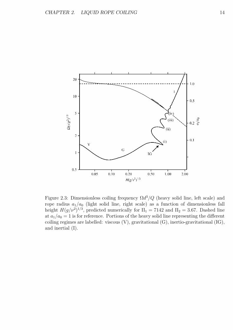
regimes characterized by different force balances in the coil. Fig. 2.3 shows how these

regimes show up in curves of Ω(H) , the frequency of coiling and a1(H) the radius of

the rope, for one set of experimental parameters. These curves were determined by

solving numerically the thin-rope equations of Ribe (2004). In Fig. 2.3 for simplicity,

we neglected surface tension, which typically modifies the coiling frequency by no

more than a few percent for a surface tension coefficient γ ≈ 21.5 dyne cm−1 typical

of silicone oil. We have included surface tension effect in most of our numerical

calculations. Surface tension is however important in related phenomena such as the

thermal bending of liquid jets by Marangoni stresses (Brenner & Parachuri 2003).

We observe that different modes of coiling are possible, depending on how the

three forces in the coil are balanced. For small dimensionless heights H(g/ν2)1/3 <

0.08, coiling occurs in the viscous (V) regime, in which both gravity and inertia are

negligible and the net viscous force on each fluid element is zero. Coiling is here

driven entirely by the injection of the fluid, like toothpaste squeezed from a tube.

Because the jet deforms by bending and twisting with negligible stretching, its radius

is nearly constant, Therefore, a1 ≈ a0 and U1 ≈ U0. Fig. 2.4 (a,e). We observe that,

for very small height the rope is slightly compressed against the fluid pile as shown

in Fig. 2.5.


Figure 2.3: Dimensionless coiling frequency Ωd3/Q (heavy solid line, left scale) andrope radius a1/a0 (light solid line, right scale) as a function of dimensionless fallheight H(g/ν2)1/3, predicted numerically for Π1 = 7142 and Π2 = 3.67. Dashed lineat a1/a0 = 1 is for reference. Portions of the heavy solid line representing the differentcoiling regimes are labelled: viscous (V), gravitational (G), inertio-gravitational (IG),and inertial (I).


Figure 2.4: Different coiling regimes. (a) Viscous regime: coiling of silicone oil withν = 1000 cm2/s, injected from an orifice (top of image) of radius a0 = 0.034 cmat a volumetric rate Q = 0.0044 cm3/s. Effective fall height H = 0.36 cm. (b)Gravitational regime: coiling of silicone oil with ν = 300 cm2/s, falling from anorifice of radius a0 = 0.25 cm at a flow rate Q = 0.093 cm3/s. Fall height is 5 cm.The radius of the portion of the rope shown is 0.076 cm. (c) Inertial regime: coiling ofsilicone oil with ν = 125 cm2/s, a0 = 0.1 cm, Q = 0.213 cm3/s and H = 10 cm. Theradius a1 is 0.04 cm. (e)-(g) Jet shapes calculated using Auto97 (Doedel et al. 2002)for three modes of fluid coiling [19]. (e) Viscous coiling. (f) Gravitational coiling. (g)Inertial coiling.


Figure 2.5: Rope of silicon oil with ν = 1000 cm2/s, injected from an orifice ofradius a0 = 0.034 cm at a volumetric rate Q = 0.0044 cm3/s and effective fall heightH = 0.30 cm. is slightly compressed against the plate, so the diameter at bottom islarger than the diameter of the filament near the nuzzle.

Dimensional considerations (Ribe 2004) and the general relation Ω ∼ U1/R then

imply

R ∼ H , ΩV =Q

Ha21

. (2.5)

After the viscous coiling regime, 0.08 ≤ H(g/ν2)1/3 ≤ 0.4, when inertia is negli-

gible, viscous forces in the coil are balanced by gravity (FG ≈ FV ≫ FI), giving rise

to gravitational (G) coiling. Fig. 2.4(b,f). The scaling laws for this mode are (Ribe

2004)

ρνa41U1R

−4 ∼ ρga21 (2.6)

R ∼ g−1/4ν1/4Q1/4 ≡ RG, Ω ∼ g1/4ν1/4a−21 Q3/4 ≡ ΩG (2.7)

which is identical to the typical frequency for the folding of a rope confined to a

plane (Skorobogatiy and Mahadevan 2000). The rope’s radius is nearly constant

(a1 ≈ a0) at the lower end (0.08 ≤ H(g/ν2)1/3 ≤ 0.15) of the gravitational regime,

implying the seemingly paradoxical conclusion that gravitational stretching in the

tail can be negligible in “gravitational” coiling. This apparent paradox is resolved

by noting that for a given strain rate, the viscous forces associated with bending and

twisting of a slender rope are much smaller than those that accompany stretching.


The influence of gravity is therefore felt first in the (bending/twisting) coil and only

later in the (stretching) tail, and thus can be simultaneously dominant in the former

and negligible in the latter.

When the height gradually increases to H(g/ν2)1/3 ≈ 1.2, a third mode, ‘inertial’

coiling is observed. (Fig. 2.4(c,g)). Viscous forces in the coil are now balanced almost

entirely by inertia (FI ≈ FV ≫ FG), giving rise to inertial (I) coiling with this scaling

law: (Mahadevan et al. 2000)

ρνa41U1R

−4 ∼ ρa21U

21 R−1. (2.8)

The radius and frequency for this mode are proportional to

R ∼ ν1/3a4/31 Q−1/3 ≡ RI , Ω ∼ ν−1/3a

−10/31 Q4/3 ≡ ΩI . (2.9)

For 0.4 ≤ H(g/ν2)1/3 ≤ 1.2, viscous forces in the coil are balanced by both gravity

and inertia, giving rise to a complex transitional regime “inertio-gravitational” (IG)

The curve of frequency vs. height is now multivalued. We will concentrate on this

part in the next chapter and only discuss the results for the three ”pure” regimes

here.

2.4 Frequency versus height

2.4.1 Viscous-Gravitational Transition

Fig. 2.6(a) shows the angular coiling frequency Ω (circles) as a function of height

measured using the first setup with Q = 0.0038 cm3/s. The frequency decreases as

a function of height for 0.25 < H < 0.8 cm, and then saturates or increases slightly

thereafter. The behavior for 0.25 < H < 0.8 cm is in agreement with the scaling

law 2.5 for viscous coiling, which predicts Ω ∝ H−1, shown as the dashed line in Fig.


2.6(a). For comparison, the solid line shows the coiling frequency predicted numeri-

cally for the parameters of the experiment, including the effect of surface tension. The

trends of the numerical curve and of the experimental data are in good agreement,

although the latter are 15%-20% lower on average for unknown reasons. The rapid

increase of frequency with height predicted by the numerical model for H < 0.25 cm

corresponds to coiling states in which the rope is strongly compressed against the

plate. We were unable to observe such states because the rope coalesced rapidly with

the pool of previously extruded fluid flowing away from it.

In this regime, the coiling frequency is independent of viscosity and depends only

on the geometry and the flow rate even though the fluid’s high viscosity is what

makes coiling possible in the first place (water does not coil). The physical reason for

this rather surprising behavior is that the velocity in the rope is determined purely

kinematically by the imposed injection rate. This ceases to be the case for fall heights

H > 0.8 cm for which the influence of gravity becomes significant, as we demonstrate

below.

Now we want to rescale the axes of the frequency-height curve to obtain a universal

curve for viscous-gravitational transition. We anticipate that the control parameter

for this transition will be the ratio of the characteristic frequencies ΩG and ΩV of

the two modes, defined by equations 2.7 and 2.5. Accordingly, a log-log plot of

Ω/ΩV versus ΩG/ΩV = H(g/νQ)1/4 should give a universal curve, where viscous and

gravitational coiling are represented by segments of slope zero and unity, respectively.

To test this, we compare all of the experimental data obtained using the first setup

with the theoretically predicted universal curve in Fig. 2.7 (a). Segments of slope

zero and unity are clearly defined by the rescaled measurements, although the latter

are again 15%-20% lower than the numerical predictions.

2.4.2 Gravitational-Inertial Transition

For larger fall heights, both gravitational and inertial forces are important. Fig.

2.6(b) shows the frequency versus height curve measured using the second setup

with Q = 0.094 cm3/s. As we will see below, the low frequencies correspond to


Figure 2.6: Curves of angular coiling frequency vs fall height showing the existenceof four distinct coiling regimes: Viscous V , gravitational G, inertio-gravitational IG,and inertial I. Experimental measurements are denoted by circles and numerical cal-culations based on slender-rope theory by solid lines. Error bars on the experimentalmeasurements of Ω and H are smaller than the diameter of the circles in most cases.The typical appearance of the coiling rope in the V, G, and I regimes is shown by theinset photographs. a) Slow inertia-free coiling with ν =1000 cm2/s, a0 = 0.034 cm,and Q = 0.0038 cm3/s. The dashed line shows the simplified viscous coiling scalinglaw 2.5. b) High-frequency coiling with ν =300 cm2/s, a0 = 0.25 cm, and Q = 0.094cm3/s. The dashed line shows the inertial coiling scaling law 2.9.


gravitational coiling, and the high frequencies to inertial coiling. These data show

two remarkable features. First, and contrary to what happens in the viscous regime,

the coiling frequency increases with increasing height. Second, there appears to be a

discontinuous jump in the frequency at H ≈ 7 cm, we will discuss it in detail in next

chapter.

The increase of frequency with height in the inertial regime can be understood

qualitatively as follows. From equation 2.9, we expect Ω ∝ a10/3

1 in the inertial regime.

The (a priori unknown) radius a1 is in turn controlled by the amount of gravitational

thinning that occurs in the ‘tail’ of the falling rope, above the helical coil. Now the

dominant forces in the coil and in the tail need not be the same: indeed, in many of

our inertial coiling experiments, inertia is important in the coil but relatively minor

in the tail, where gravity is balanced by viscous resistance to stretching. In the limit

a1 ≪ a0 corresponding to strong stretching, this force balance (Ribe 2004) implies

a1 ∝ (Qν/g)1/2H−1, (2.10)

which when combined with equation 2.9 yields:

ΩI ∝ H10/3, (2.11)

which is shown by the dashed line in Fig. 2.6 (b), and is in reasonable agreement

with the experimental measurements. The latter agree still more closely with the full

numerical solution (solid line), which includes additional terms that were neglected

in the simple scaling analysis leading to equation 2.11. The steady decrease in the

slope of Ω(H) for H > 20 cm is due to the increasing effect of inertia in the tail of

the rope, which inhibits gravitational stretching and increases a1 relative to the value

predicted by equation 2.10.

By the same way as viscous-gravitational transition, there should exist a universal

curve describing the transition from gravitational to inertial coiling as H increases.

Fig. 2.7(b) shows a log-log plot of Ω/ΩG versus ΩI/ΩG for our experimental data

(symbols), together with the numerical prediction (solid line). The agreement is


Figure 2.7: a) Transition from viscous to gravitational coiling. Rescaled coiling fre-quency using the scales ΩV and ΩG, for an experiment performed using the low-frequency setup with ν = 1000 cm2/s, d = 0.068 cm, and Q = 0.0038 cm3/s(circle),Q = 0.0044 cm3/s (squares). Solid line: prediction of the slender-rope nu-merical model for ν = 1000 cm2/s, d = 0.068 cm, and Q = 0.0038 cm3/s. Numericalpredictions for Q = 0.0044 cm3/s is very similar and close to this curve. Portionsof the solid curve with slopes zero (left) and unity (right) correspond to viscous andgravitational coiling, respectively. Error bars primarily reflect uncertainty in estima-tion of a1. b) Transition from gravitational to inertial coiling. Rescaled parametersusing the scales ΩG and ΩI . Results are shown for experiments with ν = 300 cm2/s,d = 0.5 cm, Q = 0.094 cm3/s (circles), 0.085 cm3/s (squares) and 0.104 cm3/s (tri-angles). Solid line: prediction of the slender-rope numerical model for ν =300 cm2/s,a0 = 0.25 cm, and Q = 0.094 cm3/s. Numerical predictions for Q = 0.085 and 0.104cm3/s is very similar and close to this curve. Portions of the solid curve with slopeszero and unity correspond to gravitational and inertial coiling, respectively.


very good, especially in the transition regime between gravitational coiling (constant

Ω/ΩG) and inertial coiling (Ω/ΩG ∝ ΩI/ΩG). Evidently the gravitational-inertial

transition, such as the viscous-gravitational one, can be rescaled in such a way that

the behavior is universal.

2.5 Prediction of the Coiling Frequency of Honey

at the Breakfast Table

We conclude by using our results to predict the frequency of inertial coiling of honey

on toast. Fig. 2.8 (a). For typical viscosity and falling height of honey on toast at

breakfast table the coiling usually happens in inertial regime. A complete scaling

law for the frequency in terms of the known experimental parameters is obtained by

combining the inertial coiling law Ω ∼ 0.18ΩI with a numerical solution for a1 valid

when a1 ≪ a0 . Ribe’s calculations [31] yields:

Ω = 0.0135g5/3Q−1/3ν−2[H

K(gH3/ν2)]10/3 (2.12)

Where the function K is shown in Fig. 2.8 (b). To test this law, we measured

the coiling frequency of honey (ν = 350 cm2/s) falling a distance H = 7 cm at a rate

Q= 0.08 cm3/s onto a rigid surface. The measured frequency was 16 s−1, while that

predicted with the help of equation 2.12 is 15.8 s−1.

2.6 Radius of the Coil and the Rope

The equation (2.1) shows that the forces per unit length acting on the rope depend

critically on the radius R of the coil and the radius a1 of the rope within the coil.

Here we present a systematic series of laboratory measurements of R and a1, and

compare them to the predictions of Ribe’s slender-rope numerical model (Appendix).

Most previous experimental studies of liquid rope coiling have focussed on measuring


Figure 2.8: Examples of liquid rope coiling. (a) Coiling of honey (viscosity ν = 60cm2/s) falling a distance H = 3.4 cm. (b) Function K in equation 2.12. K(x →∞) ∼

(2x)1/4/(√

3π)

the coiling frequency. Only a few experiments [17, 31] have measured the radius a1 in

addition, and none (to our knowledge) has presented measurements of the coil radius

R.

The measurements we present here were obtained in eight experiments with dif-

ferent values of ν, d, and Q [32].

2.6.1 Radius of the Coil

Fig. 2.9 shows the coil radius R as a function of the height for the eight experiments.

The agreement between the measured values and the numerics (with no adjustable pa-

rameters) is very good overall. The coil radius is roughly constant in the gravitational

regime, which is represented by the relatively flat portions of the numerical curves

at the left of panels b, c, d, e, g, and h. The subsequent rapid increase of the coil

radius with height corresponds to the beginning of the inertio-gravitational regime.

At greater heights within the inertio-gravitational regime, the coil radius exhibits a

multivalued character similar to the one we have already seen for the frequency (e.g.,

Fig. 2.6 b).


H (mm)2R

(mm

)0 50 100 150

0

1

2

3

4

5

6

7

8

9

10

11

12

13

14

a

H (mm)

2R(m

m)

0 50 100 1500

1

2

3

4

5

6

7

8

9

10

11

12

13

14

b

H (mm)

2R(m

m)

0 50 100 150 2000

2

4

6

8

10

12

14

16

18

20

c

H (mm)

2R(m

m)

0 50 100 150 2000

2

4

6

8

10

12

14

16

18

20

d

H (mm)

2R(m

m)

0 50 100 150 2000

1

2

3

4

5

6

7

8

9

10

11

12

13

14

15

e

H (mm)

2R(m

m)

0 10 20 30 400

1

2

3

4

5

6

f

H (mm)

2R(m

m)

0 50 100 1500

1

2

3

4

5

6

7

8

9

10

11

12

13

14

15

g

H (mm)

2R(m

m)

0 50 100 1500

1

2

3

4

5

6

7

8

9

10

11

12

13

14

15

h

Figure 2.9: Coil diameter 2R as a function of height for eight experiments withdifferent values of (Π1, Π2). a: (297, 2.8), b: (465, 2.35), c: (1200, 2.08), d: (1742,2.99), e: (3695, 2.19), f: (7143, 3.67), g: (9011, 3.33), h: (10052, 3.18). The circlesand the solid line show the experimental measurements and the predictions of theslender-rope numerical model, respectively. Surface tension effect was included innumerical calculations for these experiments.


2.6.2 Diameter of the rope

The structure of the curves a1(H) (Fig. 2.10) is much simpler, showing in most cases

a monotonic decrease as a function of height that reflects the increasing importance

of gravitational stretching of the falling rope. The only significant departures from

the simple structure are the rapid decrease of a1 as a function of H in the viscous

regime (leftmost portions of panels f and g) and a small degree of multivaluedness

in the inertio-gravitational regime. The agreement between the measured values and

the numerics is good, although the latter tend to be somewhat lower than the former

on average.

The decrease of a1 is due to gravitational stretching of the tail with negligible

vertical inertia, even in the “inertial” regime 1.2 ≤ H(g/ν2)1/3 ≤ 2. Again, the

apparent paradox is resolved by noting that inertia, like gravity, can be simultaneously

dominant in the coil and negligible in the tail. Vertical inertia eventually becomes

important in the tail as well when H(g/ν2)1/3 exceeds a value ≈ 3.

2.7 Secondary Buckling

In the high-frequency inertial regime, the rapidly coiling rope can pile up to a great

height, forming a hollow fluid column whose length greatly exceeds the rope diameter.

When the height of the column exceeds a critical value Hc, it collapses under its own

weight (Fig. 2.11), and the process then repeats itself with a well-defined period that

greatly exceeds the coiling period. We call this phenomenon ‘secondary buckling’, as

opposed to the ‘primary’ buckling that is responsible for coiling in the first place.

As a first step towards a physical understanding of secondary buckling, we apply

dimensional analysis to measurements of the critical height from 13 different labora-

tory experiments with fixed kinematic viscosity ν, the surface tension coefficient γ,

diameter of orifice d, the flow rate Q and different height from orifice to pile of fluid.

The critical buckling height Hc can depend on the fluid density ρ, the kinematic

viscosity ν, the surface tension coefficient γ, the coil radius R, the rope diameter

d1 ≡ 2a1, and the flow rate Q, or (equivalently) the effective velocity U0 ≡ Q/2πd1R


0 50 100 1500

0.2

0.4

0.6

0.8

1

1.2

1.4

1.6

1.8

2

a

H (mm)

a1(m

m)

20 40 60 80 1000

0.2

0.4

0.6

0.8

1

1.2

1.4

1.6

b

H (mm)

a1(m

m)

30 60 90 120 1500

0.5

1

1.5

2

2.5

c

H (mm)

a1(m

m)

50 75 100 125 1500

0.2

0.4

0.6

0.8

1

1.2

1.4

d

H (mm)a1(m

m)

50 100 1500

0.2

0.4

0.6

0.8

1

e

H (mm)

a1(m

m)

0 10 20 30 400

0.1

0.2

0.3

0.4

0.5

0.6

f

H (mm)

a1(m

m)

0 50 100 150 2000

0.1

0.2

0.3

0.4

0.5

0.6

0.7

0.8

0.9

1

g

H (mm)

a1(m

m)

20 40 60 80 100 120 1400

0.1

0.2

0.3

0.4

0.5

0.6

0.7

h

H (mm)

a1(m

m)

Figure 2.10: Rope radius a1 within the coil as a function of height, for the sameexperiments as in Fig. 2.9.


Figure 2.11: Secondary buckling of the coil in the inertial regime, in an experimentperformed using the high-frequency setup, with ν = 125 cm2/s, d = 0.15 cm, Q =0.072 cm3/s, and H = 14 cm. Time between two photographs is nearly 0.1 s.

at which fluid is added to the top of the column. From these seven parameters four

dimensionless groups can be formed, which we take to be

G0 =Hc

d1

, G1 =νU0

gd21

, G2 =γ

ρgd21

, G3 =R

d1

. (2.13)

The groups G0, G1 and G2 are identical to those used by Tchavdarov et al [4, 33] in

their study of the onset of buckling in plane liquid sheets. Now we can write

Hc

d1

= f(G1, G2, G3), (2.14)

where the functional dependence remains to be determined.

Fig. 2.12 shows the measured values of Hc/d1 for our thirteen experiments as

functions of G1 (a), G2 (b), and G3 (c). For comparison, Fig. 2.12a also shows the

critical buckling height for plane liquid sheets [4], which is independent of the surface

tension for G1 > 20 when G2 ≤ 0.9 (the largest value of G2 considered by Yarin and

Tchavdarov [33]).

Fig. 2.12 shows that the buckling height increases with increasing the dimen-

sionless flow rate G1. The trend of the data is roughly consistent with the slope

d(lnHc)/d(lnG1) ≈ 0.2 for a planar film (solid line in Fig. 2.12a). The observed


Figure 2.12: Critical height Hc for secondary buckling as a function of the dimension-less parameters G1 (a), G2 (b), and G3 (c) defined by equation 2.13. The solid linein part (a) is the critical buckling height predicted by a linear stability analysis for aplanar film.


buckling heights also appear to increase with increasing G2 (Fig. 2.12b). This de-

pendence has no analog in the case of a planar film, for which the predicted value of

Hc at high flow rates is independent of the surface tension [33]. However, we note

that the total range of variation of the parameter R/d1 is less than a factor of 2 in

our experiments, (Fig. 2.12c), so it is difficult to infer whether the buckling height

depends on R/d1 or not.

2.8 Conclusion

In this chapter we presented experimental investigation of the coiling of a liquid rope

on a solid surface and compare these results with predictions of a numerical model for

this problem. We explained three different regimes of coiling (viscous, gravitational

and inertial) and presented the experimental measurements of frequency vs. height

in each regime. We showed that in transition from gravitational to inertial coiling,

the frequency was multivalued and could jump between two frequencies during the

time. We also presented measurements of the radii of the coil and the rope, which

were in agreement with the numerical predictions. Finally, we studied the secondary

buckling, which is the buckling of the column of the coils in high frequencies, and used

dimensional analysis to reveal a systematic variation of the critical column height as

a function of the parameters of the problem.

Chapter 3

Multivalued inertio-gravitational

regime

3.1 Introduction

The experimental observations of chapter 2 show an oscillation between two frequen-

cies at a fixed fall height near the gravitational to inertial transition. Ribe (2004)

predicted that multivalued curves of frequency vs. height should be observed when

coiling occurs in the gravitational-to-inertial transitional regime corresponding to in-

termediate fall heights.

According to Fig.2.3 for 0.4 ≤ H(g/ν2)1/3 ≤ 1.2, the viscous forces in the coil are

balanced by both gravity and inertia, giving rise to a complex transitional regime.

The curve of frequency vs. height is now multivalued, comprising a series of roughly

horizontal “steps” connected by “switchbacks” with strong negative slopes. For the

example of Fig. 2.3, up to five frequencies are possible at a given height. Near the

turning points, the frequency obeys a new “inertio-gravitational” (IG) scaling.

In this chapter we seek systematically characterize the multivalued regime of liquid

rope coiling using a combination of laboratory experiments and compare with the

results of Ribe.

30

CHAPTER 3. MULTIVALUED INERTIO-GRAVITATIONAL REGIME 31

3.2 Experimental Methods

We have used the first setup (Fig.2.2 a) and the working fluids were different silicone

oils (ρ = 0.97 g cm−3, ν = 125, 300, 1000 or 5000 cm2 s−1, γ = 21.5 dyne cm−1).

The flow rate Q was determined to within ±4.5% by recording the volume of fluid in

the syringe as a function of time. This technique permitted access to portions of the

(Π1, Π2) plane that are hard to reach with free (gravity-driven) injection. The coiling

frequency was determined by counting frames of movies taken with a CCD camera

(25 frames s−1), this method allows us to measure the frequency for the experiments

that oscillate between different states. For each point (Π1, Π2) investigated, separate

sets of measurements were obtained by increasing and decreasing the height over the

range of interest, and in one case additional measurements were made at randomly

chosen heights. The raw fall heights were corrected by subtracting the height of the

pile of fluid on the plate beneath the coil. This ensures proper comparability with

the numerical solutions, in which no pile forms because the fluid laid down on the

plate is instantaneously removed. To avoid unintentional bias, the experiments were

performed and the fall heights corrected before the corresponding curve of frequency

vs. height was calculated numerically. The effect of surface tension was included in

all numerical calculations.

A disadvantage of forced injection is that unwanted “die-swell” [37] occurs in some

cases as the fluid exits the orifice. The radius of the tail then varies along the rope in a

way significantly different than that predicted by our numerical model. Die-swell was

negligible in all the experiments with ν = 1000 cm2 s−1, but significant (≈ 10− 15%

increase in radius) in some experiments performed with lower viscosities. Here we

report only experiments for which die-swell did not exceed 10%.

For fall heights within a certain range, we observed two, three or even four different

steady coiling states with different frequencies, each of which persisted for a time

before changing spontaneously into one of the others (Fig. 3.3).


Figure 3.1: Regimes of liquid rope coiling. The symbols show experimental observa-tions of the coiling frequency Ω as a function of the fall height H for an experimentperformed using viscous silicone oil (ρ = 0.97 g cm−3, ν = 1000 cm2 s−1, γ = 21.5dyne cm−1) with d = 0.068 cm and Q = 0.00215 cm3 s−1 [34]. The solid line is thenumerically predicted curve of frequency vs. height for the same parameters. Por-tions of the curve representing the different coiling regimes are labeled: viscous (V),gravitational (G), inertio-gravitational (IG), and inertial (I).

3.3 Inertio-Gravitational Coiling

According to Fig. 2.3 and Fig. 3.1 between the gravitational and inertial parts of the

curve of frequency vs. height there is a region in which the frequency is multivalued,

comprising a series of roughly horizontal “steps” connected by “switchbacks” with

strong negative slopes. The curve exhibits four turning points (labelled i − iv in

Fig. 2.3) where it folds back on itself. The additional “wiggles” at larger values

of H(g/ν2)1/3 are not turning points because the slope of the curve always remains

positive. For the example of Fig. 2.3, up to five frequencies are possible at a given

height, three of them on the roughly horizontal steps and two others on the switchback

lines.


Near the turning points, the frequency obeys a new “inertio-gravitational” (IG)

scaling: unlike the first three regimes, the frequency of IG coiling is determined by

the balance of forces acting on the long tail portion of the rope above the coil, which

behaves like a whirling viscous string that deforms primarily by stretching, gravity,

centrifugal inertia, and the viscous forces that resist stretching are all important here,

and coiling at a fixed height can occur with different frequencies [34].

3.3.1 Experimental Observations

In the laboratory, coiling in the inertio-gravitational regime is inherently time depen-

dent, taking the form of aperiodic oscillation between two quasi-steady states with

different frequencies for a given fall height. Such an oscillation occurs, e.g., at H ≈ 7

cm in the experiment of Fig. 2.6(b). The typical appearances of the two quasi-steady

states are shown in Fig. 3.2. Note first that the coil radius R = U1/Ω is always smaller

for the state with the higher frequency, because the axial velocity U1 of the rope being

laid down (which depends only on the fall height) is nearly the same for both states.

Moreover, the pile of fluid beneath the coil is taller at the higher frequency, because

rope laid down more rapidly can mount higher before gravitational settling stops its

ascent. This is because the pile height is controlled by a steady-state balance between

addition of fluid (the coiling rope) at the top, and removal of fluid at the bottom by

gravity-driven coalescence of the pile into the pool of fluid spreading on the plate.

The coalescence rate increases linearly with the pile height, and the rate at which

fluid addition builds up the pile (≡ Q/4πRa1) is larger for the high-frequency state.

The height of the pile must therefore also be larger for this state.

The origin of the time-dependence of inertio-gravitational coiling is revealed by

the curves of Ω(H) for steady coiling. The coexistence of two or more states at the

same fall height reflects the multivalued character of the curve of frequency vs height,

which is illustrated in more detail in Fig. 3.1. The symbols show coiling frequencies

measured in an experiment performed using viscous silicone oil (ρ = 0.97 g cm−3,

ν = 1000 cm2 s−1, γ = 21.5 dyne cm−1) with d = 0.068 cm and Q = 0.00215 cm3 s−1

[34], and the solid line shows the curve of frequency vs height predicted numerically


Figure 3.2: Coexisting coiling states in an experiment with ν = 300 cm2/s, Q =0.041 cm3/s, d = 1.5 mm and H = 4.5 cm. (a) low-frequency state; (b) high-frequency state.

for the same parameters by Ribe [19]. The numerically predicted frequencies of these

steady states are in fact identical to the frequencies of the two quasi-steady states

observed in the laboratory.

3.3.2 Time dependence of IG coiling and transition between

states

Here we investigate the time-dependence of inertio-gravitational coiling in more detail,

focusing on the multiplicity of the coexisting states and the fine structure of the

transitions between them. We begin by noting that the multivaluedness of a given

curve Ω(H) can be conveniently characterized by the number N of turning (fold)

points it contains. Here we define turning points as points where dΩ/dH = ∞ and

d2Ω/dH2 > 0; thus N = 2 for the solid curve in Fig. 2.6(b). Ribe showed [34] that

N is controlled primarily by the value of the dimensionless parameter Π1 scaling as

N ∼ Π5/321 in the limit Π1 → ∞. The experiment of Fig. 2.6(b) has Π1 = 313,

which is not large enough for the multivalued character of Ω(H) to appear with

full clarity. Accordingly, we used our low-frequency setup (Fig. 2.2(a)) to perform

an experiment with ν = 1000 cm2/s and a very low flow rate Q = 0.00258 cm3/s,

corresponding to Π1 = 8490. The numerically predicted Ω(H) (Fig. 3.3 solid line)

now has N = 6, with up to 7 distinct steady states possible at a fixed fall height


Figure 3.3: Rescaled coiling frequency as a function of the rescaled fall height, for anexperiment performed using the low-frequency setup with ν = 1000 cm2/s, d = 0.068cm, and Q = 0.00258 cm3/s. Symbols: experimental measurements obtained withthe fall height increasing (squares) and decreasing (triangles). Solid line: predictionof the slender-rope numerical model. Figures show geometry of coexisting coilingstates in an experiment performed with ν = 1000 cm2 s−1, d = 0.068 cm, Q = 0.0042cm3 s−1 (Π1 = 6725, Π2 = 3.76). The total (uncorrected) fall height is 7.1 cm, andthe radius of the portion of the rope shown is 0.028 cm. left, bottom: low-frequencystate; left, top: high-frequency state; right: transitional “figure of eight” state.

(H/d ≈ 170, where d ≡ 2a0). The experimental measurements (solid symbols in Fig.

3.3) group themselves along four distinct branches or ‘steps’ that agree remarkably

well with the numerical predictions, except for a small offset at the highest step.

To our knowledge this is the first experimental observation of four distinct steps

in inerto-gravitational coiling [32]. We did not observe any coiling states along the

backward-sloping portions of the Ω(H) connecting the steps, these states seems to

be unstable to small perturbations [35]. We will investigate it more accurately by

comparing the experimental results with a linear stability analysis for these parts of

the curves, in the next sections.

The experiments also provide some insight into the mechanism of the transition


Figure 3.4: Intermediate ‘figure of eight’ state for an experiment with ν = 5000 cm2/s,Q = 0.00145 cm3/s, d = 0.068 cm , and H = 16.5 cm.

between coexisting coiling states. These occur spontaneously, and appear to be initi-

ated by small irregularities in the pile of fluid already laid down beneath the coiling

rope. In most (but not all) cases, the transition occurs via an intermediate ‘figure

of eight’ state, an example of which is shown in Fig. 3.4. During a low to high fre-

quency transition, the initially circular coil first changes to a ‘figure of eight’ whose

largest dimension is nearly the same as the diameter of the starting coil. The new,

high-frequency coil then forms over one of the loops of the ‘figure of eight’ . If the

new coil forms over the loop of the ‘eight’ that was laid down first, the sense of rota-

tion (clockwise or counterclockwise) of the new coil is the same as that of the old. If

however the new coil forms over the second loop, the sense of rotation changes.

Further understanding of the transition can be gained by measuring the coiling

frequency and the sense of rotation as a function of time (Fig. 3.5). The experimental

measurements (circles) show a clear oscillation between two states whose frequencies

agree closely with the numerically predicted frequencies of steady coiling at the fall

height in question (horizontal portions of the solid line). The oscillation is irreg-

ular, with no evident characteristic period, in agreement with the hypothesis that

transitions are initiated by irregularities in the fluid pile. The only clear trend we

were able to observe was that the low-frequency state tends to be preferred when the

coiling occurs close to the gravitational regime (i. e., for lower heights), while the


0 50 100 150 200t (s)

0

1

2

3

4

5

Fre

que

ncy

(Hz)

8 8 8

8

8 8

8

-

+

-

+ +

-

+

+

Figure 3.5: Coiling frequency as a function of time for the experiment of Fig. 3.3and H = 8.55 cm. The experimental measurements are shown by circles, and thenumerically predicted frequencies for the fall height in question are represented bythe horizontal portions of the solid line. The symbol ‘8’ indicates the appearance ofan intermediate ‘figure of eight’ state, as described in the text. The ‘+’ and ‘-’ signsindicate counter-clockwise and clockwise rotation, respectively. The oscillation shownis between the two lowest ‘steps’ in Fig. 3.3.

high-frequency state is preferred near the inertial regime (greater heights). The sense

of rotation (indicated by the symbols ‘+’ or ‘-’ in Fig. 3.5) usually changes during the

transition, but not always. All the transitions in Fig. 3.5 occur via an intermediate

‘figure of eight’ state (indicated by the symbol ‘8’), but in other experiments we have

observed the ‘figure of eight’ without any transition, as well as transitions that occur

without any ‘figure of eight’.

3.4 Whirling Liquid String Model

In pure gravitational coiling with negligible inertia the rope is nearly vertical except

in a thin boundary layer near the contact point (near the pile) where viscous forces

associated with bending are significant. As H increases, however, the displacement

of the rope becomes significant along its whole length, even though bending is still

confined to a thin boundary layer near the contact point. But at the end of gravi-

tational regime and close to the turning point in the frequency vs. height curves, it


appears that the dynamics of this regime is controlled by the tail of the rope, and

that the bending boundary layer plays a merely passive role.

We now demonstrate that the dynamics of the tail provide the key to explaining

the multivaluedness of the frequency-height curve. Numerical simulations show that

the rates of viscous dissipation associated with bending and twisting in the tail are

negligible compared to the dissipation rate associated with stretching. The tail can

therefore be regarded as a “liquid string” with negligible resistance to bending and

twisting, whose motion is governed by a balance among gravity, the centrifugal force,

and the axial tension associated with stretching. The balance of gravity and the

centrifugal force normal to the tail requires

ρgA sin θ ∼ ρAΩ2y, (3.1)

where A is the area of the cross-section of the tail, θ is its inclination from the vertical,

and y is the lateral displacement of its axis. Because y ∼ R and sin θ ∼ R/H , (3.1)

implies that Ω is proportional to the scale

ΩIG =( g

H

)1/2

, (3.2)

which is just the angular frequency of a simple pendulum.

Ribe has shown that [34] the lateral displacement y (according to Fig. 3.6) of the

axis of the string satisfies the boundary value problem:

k−1 sin k(1− s)y′′ − y′ + Ω2y = 0, y(0) = 0, y(1) finite, (3.3)

where primes denote differentiation with respect to the dimensionless arclength s =

s/H and Ω = Ω(H/g)1/2. The three terms in (3.3) represent the axis-normal compo-

nents of the viscous, gravitational, and centrifugal forces, respectively, per unit length

of the string. The dimensionless parameter k measures the degree of gravity-induced


Figure 3.6: Geometry of liquid rope coiling in the inertio-gravitational regime. ei

(i = 1, 2, 3) are Cartesian unit vectors fixed in a frame rotating with the rope, anddi are orthogonal material unit vectors defined at each point on its axis, d3 beingthe tangent vector. The parameters Q, a0, H , R, and Ω are defined as in Fig. 2.1a.Geometry of the tail, modeled as an extensible string with negligible resistance tobending and twisting. This string lies in the plane normal to e2, and d1 · e2 = 0.The lateral displacement of the axis from the vertical is y(s), where s is the arclengthmeasured from the injection point.

stretching of the string, and satisfies the transcendental equation

0 = 2B cos2 k

2− 3k2, (3.4)

where B is the buoyancy number defined as B ≡ πa20gH2/νQ. The limit k = 0

(B = 0) corresponds to an unstretched string with constant radius, whereas a strongly

stretched string has k = π (B →∞).

Equations (3.3) define a boundary-eigenvalue problem which has non-trivial so-

lutions only for particular values Ωn(k) of the frequency Ω. Fig. 3.7 shows the first


Figure 3.7: First six eigenfrequencies Ωn(k) of the boundary-value problem (3.3) fora whirling liquid string.

six of these eigenfrequencies as functions of k, Ribe has solved using AUTO 97 [34].

In the limit k = 0 we recover the classical solution for the eigenfrequencies of an

inextensible chain, which satisfy J0(2Ωn(0)) = 0, where J0 is the Bessel function of

the first kind of order 0.

To test whether these eigenfrequencies correspond to the multiple frequencies seen

in the full numerical solutions, Ribe rescale the numerically predicted curves of fre-

quency vs. height to curves of Ω/ΩIG vs. ΩG/ΩIG. On a log-log plot, these rescaled

curves should exhibit distinct segments with slopes of unity and zero, corresponding to

gravitational (Ω ∝ ΩG) and inertio-gravitational (Ω ∝ ΩIG) coiling, respectively. Fig.

3.8 shows Ω/ΩIG vs. ΩG/ΩIG for Π1 = 103, 105, and 106. As expected, the rescaled

curves clearly display a transition from gravitational coiling on the left to inertio-

gravitational coiling on the right. Moreover, the multiple frequencies in the rescaled

curves correspond very closely to the whirling string eigenfrequencies Ωn(π) in the

“strong stretching” limit k = π, the first six of which are shown by the black bars at

the right of Fig. 3.8. We conclude that a rope coiling in the inertio-gravitational mode


does indeed behave as a whirling liquid string with negligible resistance to bending

and twisting.

3.5 Comparison with experiment

We now compare the predictions of the thin-rope numerical model with laboratory

data. Fig. 3.9 shows the coiling frequency Ω measured as a function of height H for the

five points (Π1, Π2) together with curves of Ω(H) predicted numerically for the same

parameters. The observations and the numerical predictions agree extraordinarily

well for experiments (b)-(e), which were all performed with ν = 1000 cm2 s−1. The

somewhat poorer agreement for case (a) (ν = 300 cm2 s−1) is probably due to die-

swell, which was about 10% in this experiment. The measurements are concentrated

along the roughly horizontal steps of the numerically predicted curves, leaving the

“switchback” portions in between almost entirely empty. In all experiments, two

coexisting coiling states with different frequencies exist over a small but finite range

of fall heights; in experiment (b), we observed three such states at H ≈ 10.8 cm. In

experiments (a)-(d), the states observed along the first step in the curve extend right

up to the first turning point. In experiment (e), by contrast, the coiling “jumps” to

the second step before the first turning point is reached.

3.6 Resonant Oscillation of the Tail in Mutivalued

Regime

The multiple ‘spikes’ in the scaled curves of frequency vs. height in Fig. 3.8 strongly

suggest that IG coiling may reflect a resonance phenomenon. Recall that the fre-

quency of gravitational coiling is controlled by the dynamics in the ‘coil’ portion of

the rope. Therefore if the frequency set by the coil happens to be close to an eigenfre-

quency of the tail, the coil will excite a resonant oscillation of the tail. Accordingly,

the spikes in Fig. 3.8 can be interpreted as resonant oscillations that occur when


Figure 3.8: Ω/ΩIG vs. ΩG/ΩIG in the limit of strong stretching (a1/a0 ≪ 1) for(Π1, Π2) = (103, 0.316) (dotted line), (105, 0.316) (dashed line), and (106, 0.562) (solidline.) Segments of the curves representing gravitational and inertio-gravitational coil-ing are denoted by G and IG, respectively. The horizontal black bars (right) indicatethe first six eigenfrequencies of a strongly stretched (k = π) whirling liquid string(Fig. 3.7).


Figure 3.9: Comparison of experimentally measured (symbols) and numerically pre-dicted (solid lines) frequencies as functions of height for the experiments. The fluidviscosity was ν = 300 cm2 s−1 for experiment (a) and 1000 cm2 s−1 for experiments(b)-(e). Values of (Π1, Π2) for each experiment are indicated in parentheses. Mea-surements were obtained in series with H increasing (squares), decreasing (circles),and varied randomly (triangles.) Error bars on H are smaller than the size of thesymbols. Error bars on Ω, which in most cases do not exceed ±5%, have been omittedfor clarity.


0.5ΩG ≈ Ωn, where 0.5ΩG is the frequency of gravitational coiling and Ωn is one of

the whirling string eigenfrequencies shown in Fig. 3.7.

An important problem remaining to be solved is that of the stability of our nu-

merical solutions. The experiments (Fig. 3.9) show that observable states of steady

coiling in the multivalued regime are concentrated along the nearly horizontal steps

in the curve of frequency vs. height below turning points. None of the steady states

we observed lies on the steeply sloping switchback between the first two steps, and

only in two cases (Fig. 3.9a and b) did we observe states that may lie on the second

(less steeply sloping) switchback. This suggests that states along the first switchback

(at least) may be unstable to small perturbations.

3.7 Stability of Liquid Rope Coiling

As shown in Fig. 3.9, the observed frequencies in ‘inertio-gravitational’ regime are

concentrated along the roughly horizontal ‘steps’ of the Ω(H) curve, leaving the

steeper portions with negative slope ( ‘switchbacks’) empty. The absence of observed

steady coiling states along the switchbacks suggests that such states may be unstable

to small perturbations. Here we investigate this question by compering experiments

with results of a linear stability analysis that have been done by Ribe et al. [35].

Here we present the results of stability analysis for three of the laboratory exper-

iments have been shown in Fig. 3.9, [34], in each of which the coiling frequency Ω is

measured as the fall height H is varied for fixed values of the hole diameter d, the flow

rate Q, and the fluid properties ρ, ν, and γ. Each experiment is therefore defined by

particular values of the dimensionless groups Π1, Π2, Π3. The effect of surface tension

was included in numerical calculations so we need the non dimensional parameter for

the surface tension (Π3). To carry out the stability analysis for a given experiment,

Ribe et al. first calculated numerically the dimensionless frequency Ω(ν/g2)1/3 ≡ Ω of

steady coiling as a function of the dimensionless height H(g/ν2)1/3 ≡ H . This yields

a curve similar to that shown (in dimensional form) in Fig. 3.9. Next, he chose a

trial value of H , and use the ’pull/push’ procedure described in appendix, to search


Figure 3.10: Stability of steady coiling with Π1 = 1220, Π2 = 2.09, and Π3 = 0.019.The continuous curve shows the numerically calculated frequency of steady coilingas a function of height. The solid and dashed portions of the curve indicate stableand unstable steady states, respectively, as predicted using the numerical stabilityanalysis described in the text. Symbols indicate experimental measurements [34] ob-tained in series with H increasing (squares), decreasing (circles), and varied randomly(triangles.)

for unstable modes having ℜ(σ) > 0, which σ is growth rate. Then he continued any

such modes in both directions along the curve Ω(H), monitoring σ to identify the

fall heights at which ℜ(σ) becomes zero, i.e. at which the mode in question becomes

stable. By repeating this procedure for different trial values of H along the curve

Ω(H), he determined the portions of the curve that represent unstable steady states.

The results of this procedure are shown in Figs. 3.10 - 3.12 for the parameters

(Π1, Π2, Π3) corresponding to the three laboratory experiments referred to above.

In each figure, the symbols indicate experimental measurements obtained in series

with H increasing (squares), decreasing (circles), and varied randomly (triangles.)

The continuous curve in each figure shows the numerically calculated curve Ω(H) for

steady coiling, and its solid and dashed portions indicate stable and unstable steady

states, respectively. Overall, the agreement between the numerical calculations and


Figure 3.11: Same as Fig. 3.10, but for Π1 = 3690, Π2 = 2.19, and Π3 = 0.044.

the experiments is very close: the observed steady states are concentrated along

the stable portions of the calculated curves, leaving the unstable portions almost

entirely ‘unpopulated’. The only significant exceptions are the three measurements

with the highest frequencies in Fig. 3.10, which lie close to an unstable segment of

the calculated curve.

However, the growth rate of the instability along this portion of the curve is very

small (σ ≈ 0.02Ω), implying that the coiling rope executes Ω/2πσ ≈ 8 revolutions

during the time required for a perturbation to grow by a factor e. This may explain

why apparently steady states such as those in Fig. 3.10 are observed despite their

instability.

Using the Ribe et al.’s numerical results helps to explain the mechanism by which

steady coiling becomes unstable. The steady coiling solution comprises an interior

region in which bending is negligible and two boundary layers near the injection and

contact points where significant bending is concentrated. In the interior, the rope


Figure 3.12: Same as Fig. 3.10, but for Π1 = 10050, Π2 = 3.18, and Π3 = 0.048.

behaves essentially as a ‘whirling viscous string’ [34]: the lateral deflection increases

smoothly downward and the gravitational force is balanced about equally by the

viscous force associated with axial stretching and by (centrifugal) inertia. In the

lower (and more dynamically significant) boundary layer, the gravitational force is

balanced almost entirely by the viscous force associated with bending, with inertia

playing a subsidiary role. The structural features of the eigenmode are concentrated

in the lower boundary layer, where the gravitational force is balanced primarily by

viscous forces. The mechanism of the instability therefore involves a balance between

gravity and the viscous resistance of the rope to bending, with inertia playing a

secondary role. This conclusion can be verified by ‘turning off’ all the inertial terms

in the perturbation equations, while holding constant all the other parameters in the

numerical code. The instability still occurs; but the growth rate is now more than

double the ’true’ growth rate predicted by the full numerical model with all inertial

terms retained. This demonstrates that inertia is not essential to the instability, but

that it nevertheless significantly influences the growth rate.

A comparison of Figs. 3.10-3.12 raises a further question: how does the number


Ns of stable segments of the curve Ω(H) depend on the experimental parameters?

The stable segments are confined for the most part to the roughly horizontal portions

(‘steps’) of the Ω(H) curve. Ribe et al. [34] showed that the total number N of (stable

and unstable) steps in the curve scales as N ∼ Π5/321 in the limit when Π1 →∞ and

gravitational stretching of the rope is strong (a1 ≪ a0). Figs. 3.10-3.12 suggest that

Ns also increases with Π1: Ns = 2 for Π1 = 1220, and Ns = 3 for Π1 = 3690 and

10050. Moreover, the fourth step in Fig. 3.12 is only slightly unstable (σ ≈ 0.004Ω),

suggesting that Π1 = 10050 may be just below the value above which Ns = 4.

Unfortunately, numerical convergence becomes difficult to achieve when Π1 and/or Ω

is too large, and we were therefore not able to determine a scaling law for Ns. For

now, we can only speculate that it scales in the same way as the total number of

steps, viz., Ns ∼ Π5/321 .

3.8 Conclusion

In this chapter we investigated experimentally and theoretically a curious feature of

this instability: the existence of multiple states with different frequencies at a fixed

value of the fall height. Using a numerical model based on asymptotic ‘thin rope’

theory, we determined curves of coiling frequency Ω vs. fall height H as functions

of the fluid viscosity ν, the diameter d of the injection hole, the volumetric injec-

tion rate Q, and the gravitational acceleration g. In addition to the three coiling

modes previously identified (viscous, gravitational, and inertial), we find a new mul-

tivalued “inertio-gravitational” mode that occurs at heights intermediate between

gravitational and inertial coiling. The frequencies of the individual branches are pro-

portional to (g/H)1/2, and agree closely with the eigenfrequencies of a whirling liquid

string with negligible resistance to bending and twisting. The predictions of the

numerical model are in excellent agreement with laboratory experiments. The exper-

iments further show that interbranch transitions in the inertio-gravitational regime

occur via an intermediate state with a “figure of eight” geometry that usually changes

the sense of rotation of the coiling but not always.


Comparing the experimental results with results of a linear stability analysis shows

that steady coiling in the multivalued ‘inertio-gravitational’ (IG) regime is stable only

along discrete segments of the frequency vs. height curve, the distribution of which

agrees very well with high-resolution laboratory measurements. The stability analysis

further shows that coiling is stable at all heights in the three remaining regimes

(viscous, gravitational, and inertial), in agreement with the experiments in chapter

2 [31]. Analytical theory, numerical analysis, and laboratory experiments thus come

together to offer a consistent portrait of steady coiling over the whole range of fall

heights and frequencies at which the phenomenon occurs. The dominant balance of

(perturbation) forces in the instability is between gravity and the viscous resistance

to bending of the rope; inertia is not essential, although it significantly influences the

growth rate.

Chapter 4

Spiral Bubble Pattern in Liquid

Rope Coiling

4.1 Introduction

The study of spirals in nature goes back a few centuries, when for instance Swammer-

dam was one of the first to try and describe the beautiful forms of certain seashells

[38]. The standard work on spontaneous pattern formation in Nature, Darcy Thomp-

son’s ”On Growth and Form” [38] describes a multitude of spiral patterns; besides

shells he discusses for instance spiral patterns of seeds in sunflowers, but also the

helical structure of branches or leaves on a growing plant stem. All these spirals are

self-organized, but still obey rather strict mathematical rules; shells are generally log-

arithmic spirals in which the distance between successive loops grows in a precisely

determined fashion with increasing distance from the center [39]. For phyllotaxis

(the sunflower spirals), Douady and Couder [40] have shown with a clever laboratory

experiment that the spirals form due to a self-organized growth processes: new seeds

are generated at a fixed frequency in the center and through a steric repulsion repel

each other; the maximization of the distance between the seeds then leads to a special

subtype of logarithmic spiral pattern: the golden or Fibonacci spiral.

However not all spirals in nature are due to a steric repulsion between the elements

constituting it. Over the past few years, self-organized spiral waves have been studied

extensively [41] . These dynamic spirals form spontaneously in excitable media [42, 43]

50

CHAPTER 4. SPIRAL BUBBLE PATTERN IN LIQUID ROPE COILING 51

and have been observed in systems as different as catalytic surface oxidation [44], the

Belousov-Zhabotinsky chemical reaction [45, 46, 47, 48, 49] , aggregating colonies of

slime mold [50, 51] and heart tissue where spiral waves in the contracting heart tissue

are believed to be one of the causes role in cardiac arrhythmia and fibrillation [52].

In this chapter we present a simple laboratory experiment that demonstrates the

condition for the formation of spiral waves. In previous chapters we investigated how

the frequency and radius of the coiling depends on the orifice diameter, the height of

fall, flow rate, and the fluid viscosity. We showed that there are four different regimes

of coiling that depend strongly on the height of fall. During the coiling some air can be

captured by the moving fluid and make some bubbles. In a relatively small region of

the parameter space the buckling coil will trap air bubbles in a very regular way, and

these air bubbles will subsequently form surprising and very regular spiral patterns.

We also present a very simple model that explains how these beautiful patterns are

formed, and how the number of spiral branches and their curvature depends on the

coiling frequency, the frequency of precession of the coiling center, the total flow

rate, and the fluid film thickness. The main finding is that in addition to the coiling

frequency, to get the spiral waves the center of the coil needs to precess with a second,

different frequency. We show that this is both a necessary and sufficient condition to

get Fermat’s spirals. The idea that two different frequencies is sufficient and necessary

to produce spirals was suggested theoretically (Hakim and Karma [41]) but has never

been observed experimentally, to our knowledge.

A picture of steady ’liquid rope coiling’ is shown in Fig. 4.1. Depending on the fluid

viscosity, the pile of coils can have different shapes. In viscous regime for relatively

high viscosities (ν ≈ 1000 cm2/s) the pile remains intact for several coiling periods,

becomes quite high, and has a shape like a corkscrew. For relatively low viscosities

(ν ≈ 100 cm2/s) the pile disappears within one or two coiling periods, and remains

very low. In both these cases there are no bubbles generated.

For large falling heights (H(g/ν2)1/3 ≥ 1.2) that inertial terms are important and

the frequency of coiling is very high the viscous decay time is so big compared to

the coiling time so the coiling filament forms a liquid tube that builds up, buckles

under its own weight once a certain height is reached (Fig. 2.11), and starts rebuilding


Figure 4.1: Liquid rope coiling. Depending on the fluid viscosity, the coils can eitherbuild up in a tall pile not unlike a corkscrew (a), or vanish into the bulk of the fluidwithin one coiling period (b). a) silicone oil with ν = 1000 cm2/s, injected from anorifice of radius a0 = 0.034 cm at a volumetric rate Q = 0.0044 cm3/s. Effective fallheight H = 0.5 cm, The diameter of the portion of the rope shown is 0.06 cm. b)silicone oil with ν = 125 cm2/s, falling from an orifice of radius a0 = 0.2 cm at a flowrate Q = 0.1 cm3/s. Fall height is 1.5 cm. The diameter of the portion of the ropeshown is 0.4 cm.


with a period. This second buckling traps an air bubble each time, but the patterns

formed by these bubbles are very irregular. In this case we have tow different size

for bubbles, very fine bubbles that forms during the coiling their size is less than the

radius of the filament, and large bubbles with a size comparable to the diameter of

the liquid tube. These bubbles form during the second buckling.

Inside a quite narrow region of the gravitational regime we observe the formation

of very regular and beautiful spiral patterns (Fig. 4.2). What happens is the following.

In all other regimes of coiling, the newly formed coil falls exactly on top of the one

that was laid down previously. However in the gravitational regime, there is a slight

irregularity in the position of the coils, leading to a slightly ’messy’ pile of coils. This

irregularity is due to the fact that the center of coiling tends to displace itself on a

circle of its own, clearly with a frequency that is slower than that of the coiling. It is

during the coalescence of two coils that are not exactly on top of each other that the

small air bubbles are formed, and are trapped in the liquid due to the high viscosity.

The bubbles are then advected away from the center radially by the flow, due to the

action of gravity on the pile of material (Fig. 4.3). In a small range of height in

gravitational regime the frequency of coiling and frequency of precession are in a way

that the bubbles trapped regularly and this leads to the spiral patterns.

4.2 Experimental Process

We have performed these experiments using the first setup (Fig. 2.2 a) with silicone

oils of different viscosities (ν = 100, 300, 1000, and 5000 cm2/s) but have observed

spiral patterns only for a viscosity of 300 cm2/s. We also used different orifice

diameters (d = 0.68, 1.5, 1.6, and 2.5 mm) and while we saw some irregular patterns

for an orifice of 0.68 mm with flow rate of 0.02 cm3/s and falling height of 30 mm,

clear spiral patterns were observed for the 1.5 mm and 1.6 mm orifices with flow

rates between 0.047 and 0.137 cm3/s and heights between 32 and 50 mm.


Figure 4.2: Inside a quite narrow region of the control parameter space, the coilingrope traps bubbles of air which form nice spiral patterns. Notice how the subsequentcoils are displaced with respect to each other. The diameter of the pile is about 1 cm.

Figure 4.3: The process of air trapping and bubble formation. Reflection and refrac-tion on the curved surface of the coils makes it difficult to study the details of bubbleformation, but one can still follow the dynamics as seen in this series of picturesshowing one cycle of bubble formation in two branches - one just above the center ofthe picture, and one in the upper right corner.


4.3 The Regime of Spiral Bubble Patterns

In the lowest part of the gravitational regimes there is a precession in the moving of

the coil and there are some irregular bubbles, with increasing the height the bubble

pattern become more regular and some unclear spiral pattern is observed. Increas-

ing the height make the patterns more clear and finally near the upper end of the

gravitational regime the patterns become unclear and disappear. Fig. 4.4 shows the

numerically predicted curve of frequency vs. height using Ribe’s method, for one of

the experiment and the clear spiral pattern have been observed in a range of height

between 3 to 4 cm from the orifice, before the step of frequency in the curve. At

4.5 cm from the orifice transition from low frequency level to high frequency level

observed with no regular spiral pattern, so the spiral regime happens in gravitational

before the inertio-gravitational regime. According to the numerical prediction the

frequency of coiling in spiral regime should be nearly constant.

In all of the cases that spiral have been observed, the spiral patterns have five

branches and five bubbles were generated after formation of nearly four coils. The

bubble sizes increase with increasing flow rate and also depends on the height. For

clear patterns the bubbles are larger than unclear patterns. The curvature of the

branches depend on the flow rate, the falling height, and the direction of coiling. If

the coiling direction is reversed after an external perturbation of the filament, the

curvature of the branches changes sign as seen in Fig. 4.5. Changing the height

lead to change the angular distance between every two bubbles in one branch and it

changes the shape of the branches (Fig.4.6). While the branches are curved in most

of the relevant parameter region, they can be almost straight (Fig.4.6(c)). We also

observe that the shape of the patterns depends on the stagnation flow of the pile on

the surface; if we modify the experiment by using a plane with boundaries at some

distance from the center the stagnation flow will be slower and the branches closer

together.


Figure 4.4: Angular coiling frequency Ω vs. fall height H for an experiment withν = 300 cm2 s−1, d = 1.6 mm, and Q = 0.137 cm3s−1, predicted numerically usingthe method of [19]. The symbols G and IG indicate portions of the curve correspond-ing to gravitational and inertio-gravitational (multivalued) coiling, respectively. Thedashed portion of the curve indicates steady coiling states that are unstable to smallperturbations, as determined using the method of [35]. Clear spiral patterns wereobserved in the height range H = 3−4 cm, before the turning point in the numericalcurve that marks the onset of IG coiling [34]. The experimentally measured angularfrequencies of coiling and precession were 17± 1 s−1 and 4± 1 s−1, respectively.

Figure 4.5: In rare instances the liquid rope spontaneously changes the direction ofcoiling. When this happens the curvature of the spiral pattern changes sign; (a) therope is coiling clockwise when viewed from above and the spirals are curving clockwisewhen going towards the center. (b) The coil is in the middle of changing direction.Notice the ’extra coil’ outside the pile. (c) the rope is now coiling in the counterclockwise direction and the spiral pattern is disturbed near the pile. (d) the coilingis counter clockwise and the curvature of the spiral pattern have changed sign.


Figure 4.6: Increasing the height from a to d lead to change the angular distancebetween every two bubbles in one branch and it changes the shape of the branches.In all of these experiments the coiling was in a same direction the number of branchesare 5. Photos were taken from below and the reflection of light from the glass substratelead to appear some extra branches.

4.4 A Simple Model For The Spiral Pattern For-

mation

Using the experimental observations we now present a simple model for the formation

of the spirals. The bubbles are generated because the center of coiling is not stationary

but moves a little between each coil, and air is trapped between coils displaced with

respect to each other. Subsequently the bubbles are transported radially with the

stagnation flow. This will give rise to a Fermat’s spiral (i.e. a spiral obeying r =

±aθ0.5, where r is the radius, a some constant, and θ the angle), since r ∼ t0.5 ∼ θ0.5.

To model this we assume that the coiling center moves on a circle of its own, and the

path laid down by the coiling filament is then given by

X(t) = r2 cos(2πF2t) + r1 cos(2πF1t) (4.1)

Y (t) = r2 sin(2πF2t)− r1 sin(2πF1t) (4.2)

where r2 and F2 is the radius and frequency of the circle described by the motion

of the coiling center, while r1 and F1 is the radius and frequency of coiling around

this point (Fig. 4.7). The minus sign is there because the coiling was observed to

always be in the opposite direction of the rotation of the coiling center and we want


Figure 4.7: Coiling around a center which moves on a circle of its own. r1 and F1 arethe radius and frequency of coiling, while r2 and F2 are the radius and frequency ofprecession of the coiling center. The direction of precession is in the opposite directionthan that of the coiling. Here r2/r1 = 1.43 and F1/F2 = 4,[48].

to keep F1 and F2 positive. From our experiments we find that F1/F2 and r1/r2

are both about four. If we use these values to compute the path of the filament we

observe that if F1/F2 is four exactly, the path will repeat itself after one rotation of

the bubble generator while the path will be slightly shifted for each rotation if F1/F2

is only approximately but not exactly four (Fig. 4.8). Our experimental observations

are consistent with one bubble being trapped at points 1 through 5 in Figs. 4.8, 4.9.

This means that five bubbles will be generated for each four coils which is exactly

what we observed experimentally when counting bubbles and coils. The reason for

this is that the frequency of the coiling and the frequency of the rotation of the coiling

center adds in the following way: A bubble is formed each time the vector from the

rotation center to the coiling center is parallel to the vector from the coiling center

to the filament laid down (see Fig. 4.7). That is, bubbles are formed at a frequency

identical to the frequency of the rotation of the dot product.

~r1 · ~r2 = r1r2(cos(2πF1t) cos(2πF2t) (4.3)

− sin(2πF1t) sin(2πF2t)) (4.4)

= r1r2 cos(2π(F1 + F2)t) (4.5)


So the frequency of bubble generation is F1 +F2 and the ratio of bubbles generated to

the number of coils will be (F1 + F2)/F1. For the measured value of F1/F2 ≈ 4, this

gives (F1 + F2)/F1 ≈ 5/4 just as observed. From the frequency of bubble generation

one can also predict the number of spiral branches to be n(F1+F2)/F2, where n is the

smallest natural number that makes n(F1 + F2)/F2 approximately a natural number.

The reason that n must be there is that if F1/F2 is say 4.33, then (F1 + F2)/F2

is 5.33 and it will take three rotations of the coiling center to add a bubble to all

branches and start adding to the first one again - totaling 16 branches. The reason

that n(F1 + F2)/F1 needs not exactly be a natural number is that if it is sufficiently

close, say 4.98, the bubbles will not be seen as being part of 50 branches but rather

5 branches that are slightly curved.

In order to test this model directly against our experiments we did a simple nu-

merical simulation, where we assume that the coiling center precess with frequency

F2, the coiling happens with frequency F1, and bubbles generated move radially with

a speed given by v = Q/(2πrh), where Q is the total flow rate, r the radial position,

and h the height of the fluid film. In Fig. 4.10 we show a fit of this simple model to ex-

perimental data. The measured values are: F1=2.7 Hz, F2=0.7 Hz, Q=0.047 cm3s−1,

and h=4 mm. The fitting parameters used to obtain agreement between the exper-

imental bubbles and the model are: F1=2.7 Hz, F2=0.7 Hz, Q=0.047 cm3s−1, and

h=3.6 mm, so the agreement is very good. In practice we inserted the experimentally

obtained values in the model and saw what should be changed in order to obtain the

best agreement. As we measured F1, F2, and Q we trusted those values and tried

to change only h which gave a good match at h=3.6 mm. We attribute the slight

difference between the two obtained values for h to the approximation v = Q/(2πrh).

Since the bubbles are near the top of the fluid, they will move slightly faster than the

average as assumed above. This means that the average flow speed in the model must

be slightly higher than the actual flow speed, which requires that flow takes place in

a film with a slightly lower hight than the actual height. This simple model thus pro-

vides us with a not only qualitatively but also quantitatively detailed understanding

of the formation of the spiral bubble patterns.


Figure 4.8: A model of the path laid down by the coil for the experimentally measuredvalues of r1/r2 ≈ 4 and F1/F2 ≈ 4. (a) the path exactly repeats itself when F1/F2 = 4giving rise to straight radial branches (Fig. 4.9(a), bubbles are generated at positions1, 2, 3, 4, and 5. (b) When F1/F2 = 3.9 the path is slightly displaced for eachprecession, which gives rise to curved spiral branches (Fig. 4.9)(b).

Figure 4.9: Patterns of bubbles generated at positions 1, 2, 3, 4, and 5 in Fig. 4.8. IfF1/F2 is equal 4 exactly the loop is closed and the bubble branches are radial, butif F1/F2 is only approximately 4 the loop is open and the bubble branches will becurved.


DataModel

Figure 4.10: A fit of the theoretical model for the bubble patterns to the experimentaldata. The parameters of the model are: the frequencies of coiling F1 = 2.7 Hz,F2 = 0.7 Hz, the flow rate Q = 0.137 cm3s−1, and the film height h = 3.6 mm.The corresponding values measured directly from the experiment are F1 = 2.7 Hz,F2 = 0.7 Hz, Q = 0.137 cm3s−1, and h = 4 mm.


4.5 Conclusion

In conclusion, we have shown the surprising formation of neatly ordered bubble pat-

terns due to a superposition of two frequencies. In the coiling problem these cor-

respond to the frequency of coiling and the frequency of precession of the center of

the coils. Our experiment and the simple model rather convincingly shows that the

existence of two different frequencies is sufficient to obtain such spiral patterns. This

specific spiral is a particular type of an Archemedian spiral (r = aθ1/n), namely the

Fermat’s spiral: r = aθ1/2, as for a bubble r ∼ t1/2 and θ ∼ t so that r ∼ θ1/2.

Chapter 5

Rope Coiling

5.1 Introduction

All mountaineers know that a rope held vertically with its lower end in contact with

a surface will coil spontaneously when it is dropped. The initial stage of the coiling is

just the buckling of the rope under its own weight. In general, when a solid material

buckles the subsequent non-linear evolution of the instability can occur in two ways.

If the material is very stiff, it will break : it is for this reason that the resistance

of structures to buckling and breaking is a key parameter in architecture and con-

struction engineering. If on the other hand the material is sufficiently flexible, the

structure remains intact but undergoes a large finite-amplitude deformation whose

dynamics are essentially nonlinear. In many cases, the cause of the nonlinearity is

the breakdown at large strain of an initially linear relation between stress and dis-

placement, either because the nonlinear (quadratic) terms in the elastic strain tensor

[1] become significant or because the material no longer satisfies Hooke’s law. Much

progress has been made recently in understanding these sorts of nonlinear behavior in

structures such as crumpled sheets of paper [53, 54, 55, 56] and crumpled wires [57].

The other principal cause of nonlinearity is purely geometrical: the fact that the final

(deformed) shape of the structure is unknown because it is far from that of the initial

state. This sort of nonlinearity can obtain even if the material’s elasticity is perfectly

linear and Hookean, the classic example being the large deformation of elastic rods

63

CHAPTER 5. ROPE COILING 64

and filaments described by the so-called Kirchhoff equations (for a review, see [58].)

Manifestations of the geometrically nonlinear dynamics of elastic rods include the

kinking of telephone cables on the ocean floor [59], handedness reversal in the coiled

tendrils of climbing plants [60], the supercoiling of DNA strands [61], and the steady

coiling of elastic ropes that we study here.

Some indication of the complex behavior that we might expect to find in elastic

rope coiling is provided by the analogous phenomenon of ‘liquid rope coiling’, which

we have explained in the previous chapters. In contrast to the liquid case, elastic rope

coiling has received little attention. To our knowledge, no systematic experimental

study of the phenomenon exists. The sole investigation of which we are aware is

the numerical analysis of [20], who solved a system of asymptotic “slender body”

equations for the steady coiling of a linearly elastic rope. These authors clearly

identified (their eqn. (2.4)) a coiling regime in which elastic forces are balanced by

gravity, and their Fig. 1 implies the existence of a second regime in which both gravity

and inertia are negligible. However,it turns out that the terms representing inertia

(Coriolis, centrifugal, and local) in the equations of [20] all have the wrong sign, and

so their numerical results that involve inertia are incorrect.

Due to the apparent similarity of this phenomenon with liquid rope coiling, the

theoretical analysis is similar, taking into account the elastic properties of the rope

instead of fluid properties. Because in the case of a solid rope there is no gravitational

stretching, the numerical investigation should in fact be easier than the liquid coiling.

In contrast, the experiments are more difficult since the experimental parameters for

a rope are not as easily controllable as those for the fluid.

In this chapter we present an experimental study of the coiling of elastic ropes

falling onto (or being pushed against) a solid surface then we compare our experi-

mental results with a numerical model [62], that is similar to [20] but with all the

signs corrected. Our results show that coiling can occur in three distinct regimes -

elastic, gravitational, and inertial - depending on how the elastic forces that resist

the bending of the rope are balanced. Moreover, we find that the inertial regime

comprises two distinct limits in which the rope’s nearly vertical upper portion sup-

ports resonant “whirling string” and “whirling shaft” eigenmodes, respectively. By


means of a scaling analysis of the equations governing steady coiling, we determine

quantitative scaling laws for the different regimes that relate the coiling radius and

frequency to the fall height, the feed rate, and the rope’s material properties. The

correctness of these laws and the rich phase diagram they imply are validated by the

excellent agreement of the experiments with the numerical predictions.

5.2 Experimental Methods

We used two different experimental setups to access the different coiling regimes. In

the first setup (Fig.5.1), ordinary rope or sewing thread was wound onto a wheel,

which was then rotated by an electric motor at a fixed rate (linear velocity on the

circumference 0.3-200 cm s−1) to feed the rope down through a hole onto a glass plate

or thick piece of paper located 2-200 cm below. The coil radius was measured using

calipers, and in some cases by counting pixels on photographs, to within 0.2 mm.

The main experimental difficulty here is that commercially available ropes have a

natural curvature equal to that of the spool onto which they are wound, and so tend

to coil with a characteristic length scale close to that of spool’s circumference. We

eliminated the natural curvature in the ropes we used either by ironing them (thin

ropes) or by wetting them with water and suspending them with a weight attached

to the lower end (for thicker ropes.)

To achieve coiling at very low fall heights, we used a second setup in which pieces

of spaghetti 24-26 cm long that had been presoftened by soaking in water were ejected

downward from a vertical glass tube. The diameters (before soaking) of the two types

of spaghetti were 1.3 mm or 1.9 mm, and 1.7 mm and 2.5 mm after soaking. The

inner diameters of the tubes containing them were 2.5 mm and 2.7 mm, respectively.

The spaghetti were loaded into the tube by placing them in water and using a syringe

to suck them up (together with a surrounding layer of water), and were then ejected

either using the syringe (for high U) or by pushing with a thin rod (to achieve lower

values of U .) In both cases, U was measured by frame counting on movies taken

with a webcam operating at 15 frames s−1 or a rapid CCD camera giving up to 1000


frames s−1. Small fall heights H were measured to within 0.2 mm from photographs,

and larger heights to within 1 mm using a ruler. The mass per unit length λ of each

rope was measured by weighing a given length of it.

5.3 Young’s Modulus Measurements

The Young’s modulus E of different ropes was measured by observing the downward

deflection of short pieces of the rope having one end clamped horizontally and the

other end free. This also provided a severe test on any spontaneous curvature of the

rope; it was verified in all cases that the deflection did not depend on the orientation

of the rope. The linear theory of elastic rods [63] predicts that

∂y4

∂l4= − gλ

EI(5.1)

I = πa4

4is the moment of inertia for rotation about an axis that coincides with

diameter and a is the radius of the rope.

According to the Fig. 5.2 and because one end is free and other end is fixed, we

have following boundary conditions:

(l = 0 : y = 0,∂y

∂l= 0)&(l = L : y = D,

∂y2

∂l2= 0,

∂y3

∂l3= 0) (5.2)

if we solve this partial deferential equation with these boundary conditions we will

have the deflection of the free end of a rod of length L is:

D =8λg

2πEa4L4 (5.3)

For each rope, we measured D to within 0.05 mm using digital calipers for several

different lengths L and then estimated E by least-squares regression of the data using

the above formula (Fig. 5.3). Table 1 shows the values of λ and E for the different

ropes we used; the error on the measurement of E is on the order of 20%. The values

tabulated for the spaghetti are those measured after soaking for 2.5 hours (smaller


Figure 5.1: The first setup for rope experiment.


Figure 5.2: Deflection of Spaghetti.

diameter) and 6 hours (larger diameter) in water at 25 C.

5.4 Experimental Observations

For most of the ropes listed in Table 1 we carried out two series of experiments: one

varying the fall height H with the feed rate U fixed, and a second varying U with

H fixed. Fig. 5.4 shows some of the typical coiling configurations we observed, and

Fig. 5.5 shows a selection of our experimental measurements of the coil radius R

as a function of H and U . Two different types of behavior are seen, depending on

whether the coiling object is spaghetti fed from very low heights (≤ 1.3 cm in Fig.

5.5) or thread fed from a height of at least several cm. For the spaghetti (Fig. 5.4 a;

open squares in Fig. 5.5), R increases with H (Fig. 5.5a) but is nearly independent

of U (Fig. 5.5b.) For threads, R also increases with height (open circles and solid

squares in Fig. 5.5 a.) However, the dependence on U is more complicated: R is first

nearly independent of U , then increases, then decreases by a factor ≈ 2, and may


Figure 5.3: Deflection vs. length for spaghetti N7, after 6 hours soaking in water,Error bars on the length and deflection are less than 0.5 mm, D = aL4 is the generalform of the solid curve that was fitted to the experimental data using Tablecurvesoftware, a = 1.2 ∗ 10−4 mm−3, R2 =0.885.

Rope Composition λ (kg m−1) d (mm) E (Pa)1 Polyester thread 0.000299 1.5 1.5×105

2 Cotton thread 0.00011 0.5 2.9×106

3 Cotton Thread 0.00011 0.5 1.5×107

4 Thick Cotton Thread 0.00024 1 8.2×105

5 Thin cotton rope 0.00237 3.35 1.9×105

6 Silk thread 0.00029 0.75 8.5×106

7 Thick cotton rope 0.02169 6.5 4.1×106

8 Cotton Thread 0.001 0.6 2×106

9 Polyester Rope 0.04 3 2×107

10 Spaghetti no. 5 0.0027 1.7 6.9×104

11 Spaghetti no. 7 0.006 2.5 5.2×104

Table 5.1: Physical property of some ropes and spaghetti; the error on the measure-ment of E is on the order of 20%.


Figure 5.4: Typical coiling configurations for some of the ropes whose physical prop-erties are listed in Table 1. The numbers on the scale in each panel indicate cm. (a)rope type 10, H = 1.2 cm, U = 26 cm/s; (b) rope type 4, H = 30 cm, U = 2.3 cm/s;(c) rope type 4, H = 80 cm, U = 100 cm/s.

even increase slightly again (open and solid circles in Fig. 5.5b.) Moreover, at high

feed rates the thread sometimes becomes unstable to an unsteady ’figure of eight’

coiling mode (Fig.5.4c) that can persist as long as the length of the thread permits,

in contrast to the transient nature of such patterns in liquid rope coiling [34, 32].

5.5 Numerical Slender-rope Model

The diversity of behavior shown in Fig. 5.5 can be understood with the help of an

asymptotic “slender rope” model. The equations we use are those of [20], but with

corrections to the sign of the inertial terms and the expression for the moment of

inertia I (≡ πd4/64) of the rope’s cross-section about a diameter. These equations

describe the steady (in the co-rotating reference frame) motion of a slender rope

acted on by gravity, inertia, and the elastic forces that resist bending, and constitute

a thirteenth-order system of ODEs in which the independent variable is the arclength

s along the rope’s axis. Because both the coil radius R and the length ℓ of the

rope between the feeding point and the contact point are unknown a priori, fifteen

boundary conditions are required. We solved the resulting two-point boundary value

problem using the continuation method described by [20].


0

5

10

1 10 100

(a)

(b)

0

5

10

15

0.1 1 10 100

Figure 5.5: Selected experimental measurements of the coil radius R. (a) R as afunction of fall height H for rope type 10 with U = 2 cm/s (open squares), rope type1 with U = 10 cm/s (solid squares), and rope type 2 with U = 10 cm/s (open circles.)(b) R as a function of feed rate U for rope type 10 with H = 1.3 cm (open squares),rope type 1 with H = 50 cm (solid circles), and rope type 2 with H = 100 cm (opencircles.) The physical properties of the ropes are listed in Table 1.


Because the numerical solutions predict the existence of resonant eigenmodes (see

below), it is natural to discuss the results in terms of the coiling frequency Ω ≡ U/R

rather than the coil radius R. Nondimensionalization of the governing equations

shows that the dimensionless coiling frequency Ω ≡ Ω(d2E/ρg4)1/6 depends only on

the dimensionless fall height H ≡ H(ρg/d2E)1/3 and the dimensionless feed rate

U ≡ U(ρ/d2g2E)1/6. Fig. 5.6 shows numerically calculated curves of Ω(H) for for

several values of U . Coiling can occur in either of three regimes, depending on how

the elastic forces that resist the bending of the “coil” portion of the rope are balanced.

Per unit rope length, the magnitudes of the elastic (E), gravitational (G), and inertial

(I) forces in the coil are

FE ≈ Ed4R−3 FG ≈ ρgd2, FI ≈ ρd2U2R−1. (5.4)

In the first regime, which we call “elastic” coiling, both gravity and inertia are neg-

ligible (FG, FI ≪ FE) and the net elastic force acting on every element of the rope

is zero. A second “gravitational” regime occurs when inertia is negligible and the

elastic forces are balanced by gravity (FG ≈ FV ≫ FI .) Finally, “inertial” coil-

ing occurs when gravity is negligible and the elastic forces are balanced by inertia

(FI ≈ FV ≫ FG.) The corresponding coiling frequencies ΩE , ΩG and ΩI can be

found by estimating the coil radius R and then using the relation Ω = U/R for con-

servation of volume flux at the moving contact point. For elastic coiling, R ∼ H . For

gravitational and inertial coiling, R is obtained from the force balances FG ≈ FE and

FI ≈ FE, respectively. The results are

ΩE ∼ UH−1, ΩG ∼ U(ρg/d2E)1/3, ΩI ∼ U2(ρ/d2E)1/2, (5.5)

The above expression for ΩE corresponds to the portions of the curves with slope

= −1 (labeled E) on the left side of Fig. 5.6. The scaling law for ΩG (equivalent to

eqn. (2.4) of [20]) corresponds to the nearly horizontal portions of the curves labeled

G at the bottom right of Fig. 5.6 (the numerics show that ΩG also depends on H , but

in a way that is too weak to be determined by scaling analysis.) Finally, the scaling


law for ΩI corresponds to the horizontal lines labeled I at the upper right of Fig. 5.6.

Fig. 5.6 reveals a surprising complexity in the inertial regime, where Ω(H) oscil-

lates about the horizontal lines defined by the expression (5.5) for ΩI . This behavior

reflects the presence of resonant eigenmodes in the “tail” of the rope that are excited

whenever one of their natural frequencies is close to the inertial frequency ΩI set by

the coil. Two limiting forms of these resonant modes can be identified. In the first

limit, represented e.g. by the rightmost portion of the curve Ω(H) for U = 1.0 in Fig.

5.6, the tail of the rope behaves as a steadily whirling elastic “string” (i.e., a rope

with zero bending resistance) under gravity. If the string is nearly vertical, its lateral

deflection r(s) satisfies the (singular) eigenvalue problem

0 = g(H − s)r′′ − gr′ + Ω2r, r(0) = 0, r(H) finite (5.6)

where primes indicate differentiation with respect to the arclength s ∈ [0, H ] measured

along the string from the feeding point s = 0. The three terms in (5.6) represent the

components perpendicular to the string’s axis of the elastic tension, the gravitational

force, and the centrifugal force, respectively. The problem (5.6), which also describes

the small oscillations of a hanging chain [63], has eigenfrequencies Ωstringn that satisfy

J0(2β) = 0, where β = Ωstringn (H/g)1/2 and J0 is the Bessel function of the first kind

of order zero. The first six eigenfrequencies Ωstringn are shown by the dotted lines with

slope −1/2 near the center of Fig. 5.6. Note the close coincidence of Ωstringn for n ≥ 5

with the segments of the curve Ω(H) for U = 1.0. Moreover, in the limit H →∞ the

frequency ΩG of the gravitational mode merges smoothly with the frequency Ωstring1

of the gravest whirling string mode.

In the second limit, the tail behaves as what Love [63] (§ 286) called a “whirling

shaft”, in which the centrifugal force is balanced by the elastic resistance to bending.

The lateral displacement of the tail now satisfies

Ed2

16ρr′′′′ = Ω2r. (5.7)


Solving (5.7) subject to the boundary conditions y(0) = y′(0) = 0 (clamped end)

and y′′(H) = y′′′(H) = 0 (free end), we find that the eigenfrequencies Ωshaftn satisfy

cos p cosh p = −1, where p2 = 4H2(ρ/d2E)1/2Ωshaftn . The first six of these eigenfre-

quencies are shown by dashed lines with slope −2 on Fig. 5.6. For n ≥ 5, Ωshaftn aligns

closely with the segments of the curves Ω(H) for U = 3.16 and 10.

The phase diagram implied by the curves Ω(H, U) in Fig. 5.6 is shown as an

inset at the upper right of the same figure. The (H, U)-plane is divided into three

broad regions representing elastic (E), gravitational (G) and inertial (I) coiling. The

inertial region in turn comprises two parts corresponding to the “whirling string” and

“whirling shaft” resonant modes, with a smooth transition between them.

5.6 Comparison With Experiment and With Liq-

uid Rope Coiling

Fig. 5.7 shows the dimensionless coiling frequencies measured in four series of exper-

iments (circles), together with the predictions of the numerical model for the same

values of H , U , λ, E, and d (solid lines.) Three of the four regimes (E, G, and Istring)

are clearly captured by the experiments, and the fourth (Ishaft) is represented by the

topmost circle in Fig. 5.7 d. The excellent agreement between the numerics and the

experiments is strong evidence for the validity of the scaling laws and the general

phase diagram presented above.

In closing, we compare the behavior of coiling elastic and liquid ‘ropes’. The pri-

mary difference between the two is that a falling liquid rope is stretched by gravity,

so that its diameter decreases downward from the hole from which it was ejected.

Allowing for this effect, however, one finds that liquid rope coiling has ‘viscous’ and

‘gravitational’ regimes that are exactly analogous to the elastic and gravitational

coiling regimes, respectively, of an elastic rope [19, 31]. Matters are somewhat more

complicated if inertia is significant. Ribe et al. [34] showed experimentally and the-

oretically that liquid ropes can support “whirling string” resonant modes analogous

to those documented here, but with eigenfrequencies that are modified by the rope’s


0.01

0.1

1

10

100

1000

0.1 1 10 100 1000 10000

0.01

0.1

1

10

0.1 1 10 100

string

shaft

1

1

1

2

= 10

3.16

1.6

1.0

0.1

0.01

0.001

621

1 6

Figure 5.6: Main portion: Dimensionless coiling frequency Ω ≡ Ω(d2E/ρg4)1/6 asa function of dimensionless fall height H ≡ H(ρg/d2E)1/3 for several values of thedimensionless feed rate U ≡ U(ρ/d2g2E)1/6. The curves for U ≥ 1.0 continue in-definitely to the right (continuations not shown for clarity.) Thick horizontal barscorrespond to the inertial frequency ΩI defined by (5.5). The first six “whirlingstring” and “whirling shaft” eigenfrequencies are indicated by dotted and dashedlines, respectively. Inset: Phase diagram for elastic coiling as a function of H andU . The coiling frequency Ω(H, U) is multivalued everywhere above the solid line.The vertical dashed line indicates the approximate location of the smooth transitionbetween elastic (E) and gravitational (G) coiling. The dashed line in the inertial (I)portion of the diagram indicates a smooth transition between “whirling string” and“whirling shaft” resonant modes.


nonuniform diameter. By contrast, there is no experimental or numerical evidence

that “whirling shaft” eigenmodes can exist on liquid ropes, probably because of vis-

cous damping. But even the whirling string modes on a liquid rope disappear if the

fall height is sufficiently great, at which point coiling occurs in the ‘pure’ inertial

regime identified by [18]. This regime has no equivalent in an elastic rope, for which

the resonant modes seen in Fig. 5.6 appear to persist (as far as one can tell from the

numerics) to arbitrarily large heights.

5.7 Conclusions

In this chapter we have investigated coiling of a falling rope using a combination of

laboratory experiments with cotton threads and softened spaghetti. we measured the

elastic modulus of the ropes by measuring the downward deflection of short pieces of

the rope having one end clamped horizontally and the other end free. This allows

to compare our experimental results with a numerical model based on asymptotic

“slender rope” theory that was introduced by Ribe [62]. We found that coiling can

occur in three distinct regimes - elastic, gravitational, and inertial - depending on how

the elastic forces that resist the bending of the rope are balanced. Moreover, we find

that the inertial regime comprises two distinct limits in which the rope’s nearly vertical

upper portion supports resonant “whirling string” and “whirling shaft” eigenmodes,

respectively. We presented a complete phase diagram for rope coiling in the fall

height-feed rate space, together with scaling laws for the coiling radius and frequency

as a function of height, feed rate, and the rope’s material properties. The validity of

these results is confirmed by the excellent agreement between the experiments and

the numerics.


0.001

0.01

0.1

1

10

0.01 0.1 1 10

0.05

0.1

1

2

0.1 1 10 0.2 1 10 50

(a) (b)

(c)

(d)

0.5

1

10

0.1 1 5

Figure 5.7: Comparison of experimentally measured (symbols) and numerically cal-culated (solid lines) coiling frequencies. The dimensionless frequency Ω, fall heightH and feed rate U are defined in the text. The symbols E, G, and I indicate elas-tic, gravitational, and inertial coiling, respectively, and the subscripts “string” and“shaft” indicate the dominant resonant mode type in the portion of the inertial regimein question. Error bars reflecting the composite (propagated) errors of Ω, H , U , λ, dand E are comparable to the symbol sizes in most cases and are omitted for clarity.(a) Rope type 10 with U = 2 cm/s; (b) Rope type 3 with U = 10 cm/s; (c) Ropetype 3 with H = 30 cm; (d) Rope type 10 with H = 1.3 cm.

Chapter 6

General Conclusion

When a falling fluid jet impacts unto a horizontal surface it buckles and starts to

coil, as one sees when playing with the spoon in the honey jar. It is a common

observation that a vertically held rope will coil spontaneously when its lower end is

in contact with a surface, and its upper end is let loose: a circular pile of rope will

form spontaneously on the surface. The coiling problem is very complicated, since

it involves the non-linear elastic behavior of the rope or the simultaneous stretching

and bending of the liquid jet. In spite of the generality of the coiling phenomenon, it

has not been studied in great detail. In this thesis we have tried to propose a detailed

experimental study of the coiling instability in viscous and elastic filaments.

A High viscosity can allow for instabilities like buckling instability, which happens

only for high viscous liquids (orders of magnitude more viscous than water with a

viscosity of ∼ 1 mPa.s). What happens when a falling fluid jet impacts unto a

horizontal surface depends profoundly on the Reynolds number. If it is above some

critical value a hydraulic jump with a region of supercritical flow is formed. If it is

decreased below this value, a less spectacular regime is encountered, where the jet

simply descends into the bulk of the fluid in a stagnation flow. Both regimes can be

seen when one turns on the water and the water falls into a sink. If the Reynolds

number is decreased further below some even lower critical value however, the jet

becomes unstable and starts buckling as one sees at the breakfast table when pouring

honey on the toast.

In chapter 2, we studied the coiling instability for a liquid thread. We report a

78

CHAPTER 6. GENERAL CONCLUSION 79

detailed experimental study of the coiling instability of viscous jets on solid surfaces.

In the experiment a viscous fluid with density ρ, kinematic viscosity ν and surface

tension γ is injected at a volumetric rate Q from a hole of diameter d = 2a0 and

then falls a distance H onto a solid surface. In general, the rope comprises a long,

nearly vertical “tail” and a helical “coil” of radius R near the plate. The motion of a

coiling jet is controlled by the balance between viscous forces, gravity and inertia. The

dynamical regime in which coiling takes place is determined by the magnitudes of the

viscous (FV ), gravitational (FG) and inertial (FI) forces. We found that the frequency

of coiling was strongly controlled by the height of fall, and changing the height lead

to transition through three different regimes of coiling (viscous, gravitational and

inertial). For small dimensionless heights H(g/ν2)1/3 < 0.08, coiling occurs in the

viscous (V) regime, in which both gravity and inertia are negligible and the net viscous

force on each fluid element is zero. Coiling is here driven entirely by the injection of

the fluid, like toothpaste squeezed from a tube. At 0.08 ≤ H(g/ν2)1/3 ≤ 0.4, when

inertia is negligible, viscous forces in the coil are balanced by gravity (FG ≈ FV ≫FI ,), giving rise to gravitational (G) coiling. When the height gradually increases to

H(g/ν2)1/3 ≈ 1.2, a third mode, ‘inertial’ coiling is observed. We present experimental

measurements of frequency vs. height in each regime and measured the radii of the

coil and the jet and compared them to a numerical calculation of the coiling. We also

describe “secondary buckling”, which is the buckling of the column of coils in the high

frequency regime, and present measurements of the critical (buckling) height of the

column. In order to physically understand secondary buckling, we apply dimensional

analysis to measurements of the critical heights of different laboratory experiments.

In the transition from gravitational to inertial coiling ( 0.4 ≤ H(g/ν2)1/3 ≤ 1.2),

the frequency vs. height was multivalued, and could jump between two frequencies

during time. In chapter 3 we investigated experimentally the coexistence of multiple

coiling states with different frequencies at a fixed value of the fall height. In addition to

the three coiling modes previously identified (viscous, gravitational, and inertial), we

found a new multivalued “inertio-gravitational” coiling mode that occurs at heights

intermediate between gravitational and inertial coiling, where the rope is strongly

stretched by gravity. The frequencies of the individual branches in the frequency vs.


height curves, are proportional to (g/H)1/2 ( the pendulum frequency), and agree

closely with the eigen frequencies of a whirling liquid string with negligible resistance

to bending and twisting. The laboratory experiments are in excellent agreement

with predictions from the numerics. Inertio-gravitational coiling is characterized by

oscillations between states with different frequencies, and we present experimental ob-

servations of four distinct branches of such states in the fall height-frequency space.

The transitions between coexisting states have no characteristic period, may take

place with or without a change in the sense of rotation, and usually but not always

occur via an intermediate figure of eight state. Based on the experimental results

we proposed that, where we have no experimental data on the frequency vs. height

curve there should be an instability. Using linear stability analysis we could subse-

quently show that the multivalued portion of the curve of steady coiling frequency vs.

height comprises alternating stable and unstable segments and steady coiling in the

multivalued ‘inertio-gravitational’ (IG) regime is stable only along discrete segments

of the frequency vs. height curve, the distribution of which agrees very well with

our measurements. The stability analysis further shows that coiling is stable at all

heights in the three remaining regimes (viscous, gravitational, and inertial), also in

agreement with the experiments.

In a relatively small region in the gravitational coiling regime the buckling coil

will trap air bubbles in a very regular way, and these air bubbles will subsequently

form surprising and very regular spiral patterns. We investigated this phenomenon

in chapter 4. Near the horizontal surface where the filament starts to coil there is a

pile of fluid, the shape and the dynamic of the pile depends on the viscosity of fluid,

the flow rate, the frequency of coiling and also on the height of fall. Depending on

system parameters there can be generation of bubbles in the pile of fluid, the size and

distribution of which depends on the dynamics of the pile. In all of the experiments

the spirals have five branches and five bubbles were generated after formation of

about four coils. The direction of coiling determines the direction of the spirals. The

curvature of the branches also depends on the height of fall and the radial speed of the

moving fluid on the substrate. We also presented a very simple model that explains

how these beautiful patterns are formed, and how the number of spiral branches and


their curvature depends on the physical parameters of the problem. In this model

we assumed that the coiling center moves on a circle of its own. Different ratios of

the radii and frequencies of coiling and precession can lead to different paths for the

filament on the substrate. When we put our experimentally measured parameters

into the model we found a path with five triangular loops that we inferred are where

the bubbles were generated. Finally we have shown that the surprising formation

of neatly ordered bubble patterns is due to a superposition of two frequencies. In

the coiling problem these correspond to the frequency of coiling and the frequency

of precession of the center of the coils. Our experiment and the simple model rather

convincingly shows that the existence of two different frequencies is sufficient to obtain

such spiral patterns. This specific spiral is a particular type of an Archemedian spiral

(r = aθ1/n), namely the Fermat’s spiral: r = aθ1/2, as for a bubble r ∼ t1/2 and θ ∼ t

so that r ∼ θ1/2.

We pursue our study considering solid ropes All mountaineers know that when a

rope is dropped it forms some coils. The initiation of this is that the rope buckles

under its own weight. In general, when a solid material buckles there are two possibil-

ities for the non-linear evolution of the buckling instability. If the material is stiff, it

will generally break and the resistance to buckling (and hence breaking) is therefore

a key parameter in architecture and construction engineering, that has consequently

been studied extensively. On the other hand, if the material is sufficiently flexible, it

will not break, but rather do what the rope does, and start coiling. The geometri-

cal non-linear elastic behavior of thin flexible rods, has attracted less attention than

the breaking problem, and this is what needs to be understood to describe ropes.

In chapter 5 we presented an experimental study of “solid rope coiling”, we studied

the coiling of both real ropes and spaghetti falling or being pushed onto a solid sur-

face. We also compared our experimental results with a numerical model based on

asymptotic “slender rope” theory. We found that coiling can occur in three distinct

regimes, ( elastic, gravitational, and inertial ) depending on how the elastic forces

that resist the bending of the rope are balanced. Moreover, we found that the inertial

regime comprises two distinct limits in which the rope’s nearly vertical upper portion

supports resonant “whirling string” and “whirling shaft” eigenmodes, respectively.


We presented a complete phase diagram for rope coiling in the fall height-feed rate

space, together with scaling laws for the coiling radius and frequency as a function of

height, feed rate, and the rope’s material properties. The validity of these results is

confirmed by the excellent agreement between the experiments and the numerics.

Appendix A

Numerical Model

A.1 Introduction:

The equations for a thin viscous rope have been derived by Entov and Yarin [22, 23],

who described the geometry of the rope’s axis using the standard triad of basis vectors

from differential geometry (the unit tangent, the principal normal, and the binormal).

Here we present the numerical model that Ribe has introduced to investigate the

coiling problem and that we have used throughout this thesis to compare to our

experimental results.

A.2 Numerical model for liquid coiling and the ho-

motopy method to solve the equations:

Using a numerical approach, Ribe [19] modelled coiling in the whole frequency range,

and found three coiling modes with different dynamics. The configuration he studied

is shown in Fig. 2.1. A fluid with kinematic viscosity ν and volumetric flow rate

Q is injected through a hole of radius a0 and falls a distance H onto a plate. It is

assumed that the jet’s point of contact with the plate rotates with angular velocity

Ω and describes a circle of radius R. In most cases, the jet consists of a long, nearly

vertical ‘tail’, which feeds fluid to a ‘coil’ next to the plate.

83

APPENDIX A. NUMERICAL MODEL 84

Figure A.1: Geometry of a viscous jet. The Cartesian coordinates of the jet’s axisrelative to an arbitrary origin O are ~x(s), where s is the arc-length along the axis. Thejet’s radius is a(s). The unit tangent vector to the jet axis is d3(s) ≡ ~x ′, and d1(s)and d2(s) ≡ d3 × d1 are material unit vectors in the plane of the jet’s cross-section.[19].

Here we present Ribe’s formulation [19] in which the basis vectors normal to the

rope’s axis are material vectors that are convected with the fluid.

To write the governing equations of the steady coiling, we consider a slender jet

whose radius is everywhere much smaller than the local radius of curvature of its

axis. This allows us to reduce the three-dimensional Navier-Stokes equations for the

flow within the jet to one-dimensional equations for a line having finite resistance to

stretching, bending, and twisting. The problem is then reduced to a steady, time-

independent motion by working in a reference frame that rotates with the coil. All

the dependent variables are then functions only of the arc-length s along the jet axis,

which ranges from s = 0 (the injection point) to s = l (the point of contact with

the plate). We denote the differentiation with respect to s by a prime. All Latin

indices range over the values 1, 2, and 3, while Greek indices range over 1 and 2 .

The Einstein summation convention over repeated indices is assumed throughout.

Figure A.1 shows an element of a slender viscous jet with variable radius a(s).

The Cartesian coordinates of the jet’s axis relative to unit vectors ei rotating with the


coil are ~x(s), defined such that (x1, x2, x3) = (0, 0, 0) is the point where the fluid is

injected. The vector e3 points up, opposite to the gravitational acceleration ~g = −ge3.

At each point on the jet’s axis, we define a set of three orthogonal unit vectors

including the tangent vector d3(s) ≡ ~x ′ and two vectors d1(s) and d2(s) ≡ d3 × d1

in the plane of the jet’s cross-section. The vectors d1 and d2 are arbitrary, but are

assumed to be material vectors rotating with the fluid. Let y1 and y2 be orthogonal

coordinates normal to the jet axis in the directions d1 and d2, respectively. The

Cartesian coordinates of an arbitrary point within the jet are then

~r(s, y1, y2) = ~x + y1d1 + y2d2 = ~x + ~y. (A.1)

The orientation of the local basis vectors relative to the Cartesian basis is described

by the matrix of direction cosines

dij ≡ di · ej =

q21 − q2

2 − q23 + q2

0 2(q1q2 + q0q3) 2(q1q3 − q0q2)

2(q1q2 − q0q3) −q21 + q2

2 − q23 + q2

0 2(q2q3 + q0q1)

2(q1q3 + q0q2) 2(q2q3 − q0q1) −q21 − q2

2 + q23 + q2

0

,(A.2)

where qi(s) are Euler parameters satisfying

q20 + q2

1 + q22 + q2

3 = 1. (A.3)

Use of the Euler parameters avoids the polar singularities associated with the more

familiar Eulerian angles. The ordinary differential equations satisfied by xi and qj are

x′

i = d3i, (A.4)


q′0 =1

2(−κ1q1 − κ2q2 − κ3q3), (A.5)

q′1 =1

2(κ1q0 − κ2q3 + κ3q2), (A.6)

q′2 =1

2(κ1q3 + κ2q0 − κ3q1), (A.7)

q′3 =1

2(−κ1q2 + κ2q1 + κ3q0), (A.8)

where ~κ ≡ κidi is the curvature vector that measures the rates of change of the local

basis vectors along the jet axis according to the generalized Frenet relation

~di′ = ~κ× di. (A.9)

The velocity of a fluid particle in the jet relative to the rotating reference frame

(to first order in the lateral coordinates y1 and y2) is

~u = Ud3 −1

2U ′~y + ~ω × ~y, (A.10)

where

~ω = κ1Ud1 + κ2Ud2 + ω3d3 (A.11)

is one-half the vorticity at the jet axis (y1 = y2 = 0), U(s)d3(s) is the velocity along

the axis, and ω3(s) is the angular velocity (spin) of the fluid about the axis. The

second term on the right-hand side of equation A.10 is the lateral velocity induced by

stretching of the axis at a rate U ′. The third term represents the velocity associated

with bending and twisting of the jet.

Because the base vectors di are convected with the fluid, their angular velocity as

they travel along the jet axis is the sum of the angular velocity ~ω of the flow and any

additional spin that is imparted to the vectors d1 and d2 when they are injected at

(s = 0). Now d1 and d2 can only be steady in the rotating frame if they are injected at


s = 0 in such a way as to follow the rotation of the jet as a whole. This is equivalent

to imparting to d1 and d2 and additional spin of magnitude −Ω, where the minus

sign accounts for the fact that e3 points up and d3(0) down. The evolution equation

for di is therefore

U ~di′ = (~ω − Ωd3)× di, (A.12)

where the left-hand side is the (steady) convective rate of change of di along the

jet axis. Substitution of the Frenet relations A.9 into A.12 yields the fundamental

condition for the steadiness of di(s):

κ3 = U−1(ω3 − Ω) (A.13)

Equation A.13 allows κ3 to be eliminated from all the equations that follow.

Equations for the global balance of force and moment in the jet are obtained by

integrating the Navier-Stokes equations over the jet’s cross-section S. The dynamical

variables that then appear are the stress resultant vector

~N ≡ Nidi =

∫

S

~σdS (A.14)

and the bending/twisting moment vectors

~M ≡ Midi =

∫

S

~y × ~σdS, (A.15)

where ~σ is the stress vector acting on the jet’s cross-section. The quantities N3, M1,

M2, and M3 measure the jet’s resistance to stretching, bending in two orthogonal

directions, and twisting, respectively. The resultants N1 and N2 are the integrals of

the shear stresses that accompany bending and twisting, and are generally small.

The integrated balance of forces per unit jet length is

ρA[~Ω × (~Ω× ~x) + 2~Ω× ~U + U ~U ′] = ~N ′ + ρA~g, (A.16)


where A = πa(s)2 is the area of the jet’s cross-section. The two terms on the right-

hand side represent the viscous force that resists deformation of the jet and the force

of gravity, respectively. The three inertial terms on the left-hand side represent the

centrifugal force, the Coriolis force and the accelerations due to variations in the axial

velocity ~U ≡ Ud3, respectively.

The integrated torque balance is

ρI ~K = ~M ′ + d3 × ~N + ρI[(~g × d3)~κ− (~κ× ~g)d3], (A.17)

where I ≡ πa4/4 is the moment of inertia of jet’s cross-section and the components

of ~K ≡ Kidi are

Kα = U(Uκα)′−ΩU ′dα3−Ω2καd3βxβ +ǫαβ3[Ωdβ3(Ωd33+2ω3)+Uκβ(Ω+ω3)], (A.18)

and

K3 = 2Uω′

3 − 2U ′(Ωd33 + ω3) + Ω2καdαβxβ + 4ǫαβ3ΩUdα3κβ. (A.19)

Four additional differential equations appear in the form of constitutive relations

for the stress resultant N3 and the moments M1, M2, and M3. The derivation outlined

in [19] yields

N3 = 3ηAU ′, (A.20)

M1 = 3ηI[(Uκ1)′ + κ2(ω3 − κ3U)], (A.21)

M2 = 3ηI[(Uκ2)′ + κ1(ω3 − κ3U)], (A.22)

M3 = 2ηIω′

3, (A.23)

where η is the dynamic viscosity. Finally, the system of equations is closed by elimi-

nating the jet radius, using the volume flux conservation relation

πa2U = Q. (A.24)


Equations A.4-A.12, A.16, A.17, and A.20-A.23 are a system of 17 first-order

differential equations with two unknown parameters (Ω and l). Ribe numerically

solved these equations with 19 boundary conditions [19], using the program Auto97,

[24, 25, 26] and found Ω as a function of H .

Auto97 implements an automatic continuation (homotopy) method, wherein a

simple analytical solution of the governing equations that satisfy some boundary con-

ditions but not all of them, and then is gradually adjusted by changing the contin-

uation parameters until the numerical solution satisfies all the boundary conditions.

Before solving, the equations and boundary conditions are non-dimensionalized.

For the liquid coiling problem the starting point is an analytical solution of the

equations for a (non-coiling) jet having the form of a quarter of a circle in the absence

of gravity and inertia, which satisfies five of the boundary conditions. Beginning

from this analytical solution with continuation parameters set to zero, the numerical

procedure consists in gradually increasing the continuation parameter until a solution

of the full coiling problem is reached. Thus ”continuation” or ”homotopy” method

is a general procedure in which an existing solution is changed slightly by varying

slightly one or more of the parameters on which it depends.[24, 27]

A.3 Linear stability analysis for instability of liq-

uid coiling in multi-valued regime :

The experiments described in detail in chapter 2 show that steady liquid coiling

can in some cases be unstable. In collaboration with Ribe, we used linear stability

analysis to investigate this instability [35], here we propose a brief explanation of

the calculation that we have used through this thesis. The basic states analyzed are

numerical solutions of asymptotic ‘thin-rope’ equations that describe steady coiling.

To analyze their stability, at first a set of general equations for an arbitrary time

dependent motion of a thin viscous rope should be derived.

The starting point of analysis is a set of equations governing the unsteady motion

of a thin viscous rope, i.e., one whose ’slenderness’ ǫ ≡ a0/L ≪ 1, where a0 is a


characteristic value of the rope radius and L is the characteristic length scale for

the variations of the flow variables along the rope. Such equations were derived by

Entov and Yarin (1984)[22], who described the geometry of the rope’s axis using

the principal normal and the binormal from differential geometry. However, such a

description leads to numerical instability when the total curvature of the axis is small.

Accordingly, we use here an alternative set of equations in which the unit vectors

normal to the rope’s axis are material vectors that rotate with the fluid [19, 34].

In order to perform a linear stability analysis of steady coiling, the equations were

written in a reference frame that rotates with angular velocity Ωe3 relative to a fixed

laboratory frame. Linearization of these equations about the steady coiling solutions

with the boundary conditions yields a boundary-eigenvalue problem of order twenty-

one that has nontrivial solutions only for particular values of the growth rate σ.

This eigenvalue problem has been solved numerically[35], again using a continuation

method implemented by AUTO 97. The basic idea (e.g., Keller [27], p. 235) is to relax

one of the homogeneous boundary conditions in order to obtain a nonzero solution

for some initial guess at the eigenvalue σ; the homogeneous boundary condition is

then reimposed gradually while forcing the solution to remain nonzero and allowing

σ to converge to the true eigenvalue. So three new adjustable real parameters βi

(i = 1, 2, 3), should be introduced into the boundary conditions which are then varied

gradually to refine an initial guess for the (possibly complex) eigenvalue σ [64]. The

problem is initialized by setting β1 = β2 = β3 = 0 and making an initial guess for

the growth rate σ. The solution procedure then comprises two steps. First, ’pulling’

β3 away from 0 to some finite value (e.g., 1) with σ fixed, letting β1 and β2 float

freely. Then β3 is ’pushed’ gradually back to 0 with β1 and β2 fixed, leaving the real

and imaginary parts of σ free to float. At the end of this process, one has both an

eigenvalue σ and the full set of associated complex eigenfunctions for the twenty-one

perturbation variables. High accuracy is ensured by solving the equations for the

steady basic state simultaneously in the same program, on the same numerical grid

as the perturbation equations. The resulting system is of order 59 (17 steady variables

plus the real and imaginary parts of 21 perturbation variables).

Bibliography

[1] L. D. Landau and E. M. Lifshitz, Theory of Elasticity, Pergamon Press, Oxford

(1959).

[2] G. I. Taylor, ”Instability of jets, threads, and sheets of viscous fluid”, Proc. Intl.

Congr. Appl. Mech. Springer (1968).

[3] J. O. Cruickshank, ”Low-Reynolds-number instabilities in stagnating jet flows”,

J. Fluid Mech. 193, 111–127 (1988).

[4] B. Tchavdarov, A. L. Yarin & S. Radev, ”Buckling of thin liquid jets”, J. Fluid.

Mech. 253, 593–615 (1993).

[5] J. O. Cruickshank & B. R. Munson, ”Viscous fluid buckling of plane and ax-

isymmetric jets”, J. Fluid Mech. (1981).

[6] J. D. Buckmaster, J. Fluid Mech., 61, 449 (1973).

[7] J. D. Buckmaster, A. Nachman, and L. Ting, ”The buckling and stretching of a

viscida”, J. Fluid Mech. 69, 1 (1975).

[8] M.F. Tome and S. McKee, Int. J. Numer. Methods Fluids 29, 705 (1999).

[9] J.R.A. Pearson, Mechanics of Polymer Processing, Elsevier, Amsterdam (1985).

[10] R. W. Griffiths & J. S. Turner, ”Folding of viscous plumes impinging on a density

or viscosity interface”, Geophys. J. 95, 397–419 (1988).

91

BIBLIOGRAPHY 92

[11] H. E. Huppert, ”The intrusion of fluid mechanics into geology”, J. Fluid Mech.

173, 557–594 (1986).

[12] M. Skorobogatiy & L. Mahadevan, ”Folding of viscous sheets and filaments”,

Europhys. Lett. 52, 532–538 (2000).

[13] J. G. Ramsay, Folding and Fracturing of Rocks, (McGraw-Hill) (1967).

[14] N. M. Ribe, ”Periodic folding of viscous sheets”, Phys. Rev. E 68, 036305 (2003).

[15] N. M. Ribe, ”A general theory for the dynamics of thin viscous sheets”, J. Fluid

Mech. 457, 255 (2002).

[16] M. Brenner & S. Parachuri, ”Thermal bending of liquid sheets and jets”, Phys.

Fluids 15, 3568–3571 (2003).

[17] L. Mahadevan, W. S. Ryu, & A. D. T. Samuel, ”Fluid ’rope trick’ investigated”,

Nature 392, 140 (1998).

[18] L. Mahadevan, W. S. Ryu, & A. D. T. Samuel, ”Correction: Fluid ’rope trick’

investigated”, Nature 403, 502 (2000).

[19] N. M. Ribe, ”Coiling of viscous jets”, Proc. R. Soc. Lond. A 460. 3223–3239

(2004).

[20] L. Mahadevan and J. B. Keller, ”Coiling of flexible ropes”, Proc. R. Soc. Lond.

A 452, 1679–1694 (1996).

[21] L. Mahadevan and J. B. Keller, SIAM J. App. Math. 55.1609 (1995).

[22] V. M. Entov and A. L. Yarin, ”The dynamics of thin liquid jets in air”, J. Fluid

Mech. 140, 91 (1984).

[23] A. L. Yarin, Free Liquid Jet and Films: Hydrodinamics and Rheology, (Wiley)

1991.

[24] Doedel, E. et al. AUTO 97: ”Continuation and bifurcation software for ordinary

differential equations” (2002). http://indy.cs.concordia.ca/auto/.

BIBLIOGRAPHY 93

[25] E. J. Doedel, H. B. Keller, and J. P. Kernevez, ”Numerical analysis and control

of bifurcation problems, Part I”, Int. J. Bifurcation and Chaos 1, 493 (1991).

[26] E. J. Doedel, H. B. Keller, and J. P. Kernevez, ”Numerical analysis and control

of bifurcation problems, Part II”, Int. J. Bifurcation and Chaos 1, 745 (1991).

[27] H. B. Keller Numerical Methods for Two-Point Boundary-Value Problems, Dover,

New York (1992).

[28] G. Barnes, & R. Woodcock, ”Liquid rope-coil effect”, Am. J. Physics 26, 205–

209 (1958).

[29] G. Barnes & R. MacKenzie, ”Height of fall versus frequency in liquid rope-coil

effect”, Am. J. Physics 27, 112–115 (1959).

[30] J. O. Cruickshank, ”Viscous fluid buckling: a theoretical and experimental analy-

sis with extensions to general fluid stability”, Ph. D. thesis, Iowa State University,

Ames, Iowa (1980).

[31] M. Maleki, M. Habibi, R. Golestanian, N. M. Ribe, & D. Bonn, ”Liquid rope

coiling on a solid surface”, Phys. Rev. Lett. 93.214502 (2004).

[32] M. Habibi, M. Maleki, R. Golestanian, N. Ribe, and D. Bonn,”Dynamics of

liquid rope coiling”, Phys. Rev. E. 74, 066306 (2006).

[33] A. L. Yarin and B. M. Tchavdarov, J. Fluid. Mech. 307, 85 (1996).

[34] N. M. Ribe, H. E. Huppert, M. Hallworth, M. Habibi, and D. Bonn, ”Multiple

coexisting states of liquid rope coiling”, J. Fluid Mech. 555, 275 (2006).

[35] N. M. Ribe, M. Habibi, and D. Bonn, ”Stability of liquid rope coiling”, Phys.

Fluids 18, 084102 (2006).

[36] Ribe N M, Habibi M, Bonn D, 2007 ”Instabilites de flambage periodique: du

laboratoire au manteau terrestre”, Reflets de la physique, in preparation (invited

contribution.)

BIBLIOGRAPHY 94

[37] R. B. Bird, C. Armstrong, O. Hasseper Dynamics of Polymeric Liquids.

[38] Darcy Thompson, On Growth and Form, Cambridge University Press.

[39] M. P. DO CARMO, Differential Geometry of Curves and Surfaces, Prentice-Hall,

Inc. Upper Saddle River, New Jersey (1976).

[40] Douady and Couder,Phys. Rev. Lett. 68, 2098 (1992).

[41] Hakim and Karma, Phys. Rev. E 60, 5073 (1999).

[42] A. T. Winfree, When Time Breaks Down, Princeton University Press, Princeton,

NJ (1987).

[43] V. S. Zykov, Modelling of Wave Processes in Excitable Media, Manchester Uni-

versity Press, Manchester (1988).

[44] S. Jakubith, H. H. Rotermund, W. Engel, A. von Oertzen, and G. Ertl, Phys.

Rev. Lett. 65, 3013 (1990).

[45] A. T. Winfree, Science 181, 937 (1973).

[46] W. Jahnke, W. E. Skaggs, and A. T. Winfree, J. Phys. Chem. 93, 740 (1989).

[47] T. Plesser et al., J. Phys. Chem. 94, 7501 (1990).

[48] G. S. Skinner and H. L. Swinney, Physica D 48, 1 (1991).

[49] A. Belmonte, Q. Ouyang, and J. M. Flesselles, J. Phys. II 7, 1425 (1997).

[50] W. F. Loomis, Dictyostelium Discoideum, A Developmental System, Academic

Press, New York (1975).

[51] F. Siegert and J. Weijer, Physica D 49, 224 (1991).

[52] The several review articles in the focus issue of Chaos 8, 1 (1998).

[53] E. Sultan and A. Boudaoud, Phys. Rev. Lett. 96, 136103 (2006).

BIBLIOGRAPHY 95

[54] D. L. Blair and A. Kudrolli, Phys. Rev. Lett. 94, 166107 (2005).

[55] G. A. Vliegenthart and G. Gompper, Nature Materials 5, 216 (2006).

[56] M. BenAmar and Y. Pomeau, Proc. R. Soc. Lond. A 453, 729 (1997).

[57] C. C. Donato, M. A. F. Gomes and R. E. de Souza, Phys. Rev. E 67, 026110,

(2003).

[58] A. Goriely and M. Tabor, Nonlinear Dyn. 21, 101 (2000).

[59] J. Coyne, IEE J. Oceanic Eng. 15, 72 (1990).

[60] A. Goriely and M. Tabor, Phys. Rev. Lett. 80, 1564 (1998).

[61] A. Balaeff, C. R. Koudella and L. Mahadevan, Proc. R. Soc. Lond. A 362,1355

(2004).

[62] M. Habibi, N. M. Ribe and D. Bonn, ”Coiling of Elastic Ropes”, submitted to

Phys. Rev. Lett..

[63] A. E. H. Love, A Treatise on the Mathematical Theory of Elasticity, Dover, New

York.

[64] Neil M. Ribe, John R. Lister and Sunny Chiu-Webster, Stability of a dragged

viscous thread: Onset of stitching in a fluid-mechanical sewing machine, Phys.

Fluids 18, 124105 (2006).

List of Publications

This thesis was based on the following publications:

1. M. Maleki, M. Habibi, R. Golestanian, N. M. Ribe, & D. Bonn, ”Liquid rope

coiling on a solid surface”, Phys. Rev. Lett. 93.214502 (2004).

2. M. Habibi, M. Maleki, R. Golestanian, N. Ribe, and D. Bonn, ”Dynamics of

liquid rope coiling”, Phys. Rev. E. 74, 066306 (2006).

3. N. M. Ribe, H. E. Huppert, M. Hallworth, M. Habibi, and D. Bonn, ”Multiple

coexisting states of liquid rope coiling”, J. Fluid Mech. 555, 275 (2006).

4. N. M. Ribe, M. Habibi, and D. Bonn, ”Stability of liquid rope coiling”, Phys.

Fluids 18, 084102 (2006).

5. M. Habibi, N. M. Ribe and D. Bonn, ”Coiling of Elastic Ropes”, submitted to

Phys. Rev. Lett.

6. N. M. Ribe, M. Habibi, and D. Bonn, ” Instabilites de flambage periodique:

du laboratoire au manteau terrestre”, Reflets de la physique,(invited contribution),

in preparation.

7. M. Habibi, P. Moller, N. M. Ribe and D. Bonn, ”Spontaneous generation of

spiral waves by a hydrodynamic instability”, submitted to Euro. Phys. Lett..

96

Resume:

Dans cette these, nous presentons une etude experimentale des instabilites de flambagehelicoıdal pour un liquide visqueux et une corde. Puis nous comparons nos resultats aun modele numerique. Nous avons reussi a mettre en evidence l’existence de trois regimesdifferents pour un filament de liquide. Nous montrons ici que dans une petite region, le flam-bage de la bobine conduit a l’emprisonnement de bulles d’air d’une maniere tres particuliere,formant ainsi des structures en spirale etonnantes. Nous presentons egalement un modelesimple qui permet d’expliquer la formation de ces structures en spirale. Nous presentonsune etude experimentale du flambage helicoıdal pour des cordes et des spaghetti soit lorsqueceux-ci sont pousses contre une surface soit lorsqu’ ils sont laisses tomber librement. Nousdemontrons qu’il existe trois regimes differents de flambage helicoıdal possibles. Nous don-nons ici un cadre experimental et theorique pour comprendre le comportement des cordesdans les differents regimes et nous expliquons la relation entre les proprietes elastiquesdes materiaux et leurs proprietes de flambage helicoıdal, en particulier avec la frequenced’embobinage. Les predictions numeriques sont en excellent accord avec les resultats desexperiences realisees.

Summary:In this thesis, we present an experimental investigation of the coiling instability in a

liquid or a solid ”rope” on a solid surface and then try to compare the results with a numer-ical model. We explain different regimes of coiling for a liquid rope (viscous, gravitationaland inertial) and present the experimental measurements of frequency vs. height in eachregime. We investigate the transition from gravitational to inertial coiling, in this regimethe frequency is multivalued and can jump between two frequencies during the time. Weshow that between any step in frequency vs. height curve we have unstable part. We reportthat in a relatively small region in gravitational coiling regimes the buckling coil will trapair bubbles in a very regular way, that form spiral patterns. We also present a very simplemodel that explains how these patterns are formed. We present an experimental study ofthe coiling of both ropes and spaghetti falling onto a solid surface. We show that threedifferent regimes of coiling are possible. We in addition provide a theoretical and numericalframework to understand and quantify the behavior of the ropes in the different regimes,the numerical predications are in excellent agreement with the experiments.

coiling instability in liquid and solid ropes

Documents