cohort, turnover, and partisan effects in critical elections
TRANSCRIPT

______________ MARCIA LYNN WHICKER is Professor of Public Administration at Rutgers University, Newark. MALCOLM E. JEWELL is Professor of Political Science at the University of Kentucky. The American Review of Politics, Vol. 14, Spring, 1993: 97-117 ©1993 The American Review of Politics
Cohort, Turnover, and Partisan Effects in Critical Elections Marcia Lynn Whicker, Rutgers University, Newark Malcolm E. Jewell, University of Kentucky We examine three alternative explanations for national policy shifts surrounding critical elections. We examine evidence for cohort, turnover, and partisan effects. Data for all congresses are used, and four critical elections�1828, 1860, 1896, and 1932�receive particular attention. The cohort and turnover hypotheses as explanations for critical election policy shifts are not supported. However, support for the partisan dominance hypothesis is strong. Political party membership and strength, rather than an influx of congressional newcomers with different socialization and characteristics, is associated with major policy swings. What causes major shifts in national policy that may be reflected in the fundamental changes in public opinion associated with critical elections? Political scientists have identified three possible factors: cohort shifts asso-ciated with leadership cycles, institutional changes resulting from turnover, and partisan changes in Congress. We use biographical data on members of Congress to examine these three factors. Political scientists have directly linked historical policy shifts to critical elections, partisan realignment, and leadership selection (Ceaser 1979, Crit-tenden 1982, Mayhew 1986, Heard and Nelson 1987, Key 1966). Beck (1979) identified three types of elections. In realigning elections, the sources of party support in the electorate undergo substantial change and the party balance usually but not always is altered. In stable alignments, little vari- ability in either partisan support or advantage occurs. In dealigning eras, party loyalties decline and party voter independence increases. We are pri- marily concerned with the policy shifts associated with critical or realigning elections here. Most scholars analyzing critical elections have focused upon 1860, 1896, and 1932, elections evoking consensus that basic partisan shifts occurred (Brady 1988). Clubb, Flanigan, and Zingale (1980) included 1828 as well, dividing periods between critical elections into years of stability immediately following the critical election and years of decay that led up to the next realignment. They identified four critical elections in which significant

98 | Marcia Lynn Whicker and Malcolm E. Jewell
partisan realignment occurred, followed immediately by periods of stability (1828-1841, 1860-1875, 1896-1911, and 1932-1947). Each stable period fol-lowing a critical election was ended by mid-sequence adjustment elections (1842, 1876, 1912, and 1948), and subsequent periods of decay (1842-1859, 1876-1895, 1912-1931, and 1948-present). Periods of stability represent a time during which the majority party purportedly can pass sweeping legisla-tion, while subsequent periods of decay, following a mid-sequence readjust-ment election, represent a deterioration of the majority party position concomitant with greater difficulty in passing a legislative program.
Cyclic Shifts in Leadership Cohorts and Critical Elections The first possible explanation for policy shifts surrounding critical elections is cyclic shifts in leadership cohorts. Henry Adams was among the earlier observers of rhythms in American politics, noting that periods of conservatism, or concern for the rights of the few, alternated with periods of liberalism, or concern for the wrongs of the many (Schlesinger 1949). Adams contended that after the Declaration of Independence, twelve years were needed to create an efficient Constitution, twelve years thereafter resulted in reaction against the new government, and the third twelve-year period in the life of the young nation brought reinvigoration. Subsequently, Arthur Schlesinger, Sr., in a thesis expanded by Arthur Schlesinger, Jr. (1986), identified shifts in leadership cohorts as a source of political cycles. In addition to those periods discussed by Adams, Schles- inger differentiated the period of Jeffersonian retreat after the War of 1812 (1812-1828) from the democratization of the Jacksonian age (1829-1841). Subsequent periods included slaveholder domination (1841-1861), the aboli-tion of slavery (1861-1869), conservative rule (1869-1901), the Progressive era (1901-1919), Republican restoration (1919-1931), and the New Deal era (1931-1947). Scholars have differed on the driving impetus that underlies political cycles. Schlesinger (1986) found that during six of the periods he identified, political trends increased democracy, while in five periods, the object was to contain democracy. Hirschman (1982) contended that periods of public in-volvement alternated with pursuit of private gain. Using public opinion data, McClosky and Zaller (1984) found vacillation between the values of capitalism (the sanctity of private property, profit maximization, and market survival of the fittest) and those of democracy (equality, freedom, social responsibility, and the general welfare.) Barber (1980) discerned 12-year presidential election cycles in the 20th Century, in which a pattern of elections emphasizing conflict, conscience, and then conciliation emerged.
Cohort, Turnover, and Partisan Effects in Elections | 99
Schlesinger (1986, 29-34) posited generational or cohort effects as causing realignments and consequent legislative redirection of national policy. Each generation has similar experiences that mold common percep-tions and outlooks. The political experiences that a generation incurs as it comes to political maturity are especially relevant. These perceptions, in turn, become the pivot responsible for historical shifts. The length of a generation has expanded from Adams� 12 year cycles, when the nation first began, to about 30 years in Schlesinger�s cycle framework. Political parties become imperfect vehicles for these cohort effects that are reflected in national leadership as well as in the citizenry at large.
Turnover and Critical Elections Institutional change within congress, particularly turnover, provides a second explanation for major policy shifts surrounding critical elections (Diamond 1976). With turnover, newcomers may arrive with different policy preferences than oldtimers. Turnover during realignment periods involves a high rate of electoral defeat, in contrast to other periods, when a higher percentage of replacements occur for other reasons (Seligman and King 1980). With the decline in electoral competitiveness, congressional turnover has diminished over the past century (Fiorina et al. 1975, Price 1971). As turnover diminished, the average number of terms served increased steadily. By 1971, 20 percent of all representatives had served 10 terms or more, although that figure dropped to about 15 percent in the 1980s (Ornstein, Mann, and Malbin 1987, 17-18). In the 1980s, less than 5 percent of the representatives who have sought reelection have been defeated. Senate incumbents were not as safe as House members. In 1976, 1978, and 1980, 40 percent of Senate incumbents were defeated, but in the next three elections the percentage of Senate incumbents defeated dropped to 14 percent (Ornstein, Mann, and Malbin 1987, 56-57). Yet, high turnover provides the crucial impetus within Congress to propel �new blood� to leadership positions, thus allowing major policy shifts to occur (Brady 1988). Seligman and King (1980) explore background data for members of Congress elected during the critical elections of 1896 and 1932, and in the noncritical elections between 1872 and 1956, and find evidence of cohort and turnover effects as sources of critical elections. They note that despite profound changes in the national social fabric, the composition of congres-sional backgrounds has remained relatively constant, heavily weighted toward lawyers, business executives, and farmers. They search for changes

100 | Marcia Lynn Whicker and Malcolm E. Jewell
independent of occupation, arguing that between alignments there is no consistent linkage between background variables, turnover, and roll-call voting, but during realignments, background factors successfully predict congressional voting behavior, indicating that new legislators elected in the midst of a realignment acted as a cohort (King and Seligman 1976). Further, during critical elections, changes in background profiles cut across party lines, affecting both parties similarly, whereas after non-realigning elections the background profiles of each party�s congressional contingent change independently of one another.
Critical Elections and the Impact of Party Partisan shifts are a third explanation for the major policy shifts sur-rounding critical elections. The impact of party on critical elections may work through and in conjunction with other factors, including public opinion and partisan economic effects. Major policy shifts of critical elections are influenced by the nature and intensity of public opinion (Kingdon 1973, Hinckley 1978). According to conventional wisdom regarding critical elec-tions, external shifts in public opinion generated by new, cross-cutting issues create new partisan alignments. These alignments result in congressional turn-over sufficient to generate policy changes. Modifying conventional wisdom somewhat, Brady (1988) has found that both issues and the shape of constituent party distribution drive critical elections and the policy changes such elections entail. A five percent shift in constituent opinion may result in policy change if the shape of the distri- bution is competitive, but may not result in policy change if the distribution is U-shaped, or non-competitive. The New Deal shift was the only clear-cut realigning election in the 20th century; public opinion distributions in subse-quent elections have been non-competitive. Others concur that competitive-ness in congressional elections has declined (Ferejohn 1977, Mayhew 1974a, Erikson 1971, 1972, Tufte 1973, Kostroski 1973). American parties, never strong and disciplined compared to their Euro-pean counterparts, have declined in importance in recent years as the role of the media in campaigning (Frantzich 1989, Hinckley 1981), PAC funding (Sabato 1985, Jacobson 1987), candidate reliance on personal rather than party campaign organizations (Pomper 1977), the advantages of incumbency (Mann and Wolfinger 1980, Baker 1989), and the number of independents all have increased. The decline in party strength, in turn, has contributed to muddled electoral linkages and results, and the absence of any recent clear-cut critical elections.

Cohort, Turnover, and Partisan Effects in Elections | 101
Economic conditions have been examined as a source of electoral change that interacts with party effects. Aggregate data show that unemployment tended to fall during Democratic presidences and increase when Republicans occupied the White House (Hibbs 1977). Other studies have found economic differences according to partisan control of the White House effective only during the first two years of an administration, with the second two years being similar across administrations (Alesina and Sachs 1988, Alesina 1988, Chappell and Keech 1988). Yet, survey data have indicated that individual voting behavior is not responsive to changes in economic outcomes (Kiewiet 1981, Kinder and Kiewiet 1979, Kramer 1983), especially in congressional midterm elections when voters moderate their retrospective tendencies in presidential years to reward and penalize presidents for economic performance (Alesina and Rosenthal 1989). Voter evaluations of partisan economic performance may be but one component of long-term party identification, along with voter approval of the incumbent administration (MacKuen et al. 1989). Separate from short-term fluctuations in party identification, these two components may form a long-term electoral variable of macropartisanship with lasting effects, but without sufficient magnitude to constitute major realignments.
Hypotheses and Data We reexamine cohort, turnover, and partisan effects as factors in re-alignments, using an expanded data base and time periods. In asserting the impact of a cohort effect, Seligman and King (1980) analyzed only two critical elections (1896 and 1932). While emphasizing the crucial role of turnover in critical elections, Brady (1988) restricted his analysis to three critical elections (1860, 1896, and 1932). Further, unlike Seligman and King, who examined noncritical presidential elections for a number of years before, between, and after the elections of 1896 and 1932, Brady examines only those elections immediately preceding and following 1860, 1896, and 1932, leaving gaping numbers of noncritical elections unexamined. Thus, turnover for only one or at most two Houses coincidental with or succeeding a critical election are reported. Finally, both Seligman and King�s and Brady�s analyses cover only the U.S. House, even though legislation resulting from critical election realign-ments must also be passed by the Senate. (Of course, it should be remem- bered that popular election of senators did not begin until 1914.) Long-term patterns may not be tested fully and even may be obscured by the focus on a limited number of critical elections (Seligman and King 1980) and by

102 | Marcia Lynn Whicker and Malcolm E. Jewell
examination of only a restricted number of years immediately before and after critical elections (Brady 1988). The data used here are a merged set drawn from the roster of U.S. congressional officeholders and biographical characteristics of the U.S. Congress, 1789-1989, covering the 1st to the 101st Congress. The data set contains variables describing congressional service and background charac-teristics for each person who has served in the U.S. Congress from March 1789 through July 1989. A record exists for every Congress in which each individual has served, as well as for each chamber in which each individual has served, constituting 41,209 cases. The three major effects tested and the periods for critical elections were measured as follows: Critical elections: Considerable disagreement exists over how to iden- tify and classify realigments (Nexon 1980, Burnham 1970, Pomper 1967). We began by using the realignments and periods of stability and decay iden- tified by Clubb et al. (1980). These were the elections of 1828, 1860, 1896, and 1932. In order to include the maximum number of Congresses (the 1st through the 101st) we have designated two other elections as critical ones: 1800 and 1968. Little consensus exists on either the timing or character of the realignment or dealignment that has been occurring in recent years. But the 1968 election coincided with a sharp increase in the proportion of voters identifying as independent and (along with the 1964 election) began the decline of Democratic strength in the Deep South. Our total universe of realigning elections, then, is six: 1800, 1828, 1860, 1896, 1932, and 1968. Cohort effects: The age of each member was recoded into 5-year ordi-nally ranked categories to explore potential cohort effects. Cohort shifts could be identified by a sudden decrease in the average age within Congress, and by increased proportions of members in younger age categories. Such shifts represent a newer, younger generation seizing the leadership helm. Turnover effects: We created a �newcomer/oldtimer� variable, to dis-tinguish newly elected members of the House and Senate who had served less than two years and had been elected in the immediately preceding national election, to measure turnover effects. While cohort shifts necessarily involve an increase in the number of newcomers, an increase in the number of newcomers does not necessarily imply a cohort effect, unless it is also accompanied by a drop in average age for members. Partisan effects: Our measurement of possible partisan effects was a straightforward examination of partisan ratios for all congresses, from the first to the 101st.

Cohort, Turnover, and Partisan Effects in Elections | 103
Findings Summary Data for All Congresses Table 1 presents summaries for the three variables of interest�age as a measure of cohort effect, newcomers, and party affliation�for all Congresses, to serve as a baseline for subsequent period analysis. The mean age for members of Congress is 50.6 years, with the Senate mean age (53.9 years) being slightly higher than the House mean age (49.7 years). The modal 5-year category is higher for the Senate (ages 50 to 54, containing 16.2 percent of all Senators) than for the House (ages 45-49, containing 18.5 percent of all congressmen). The fifteen year modal category also is higher for the Senate (45-59) than for the House (40-55).
Table 1. Summary Data for 1st to 101st Congresses
Both Chambers House Senate
Mean Age 50.6 49.7 53.9 Modal Age 5 yr. cat. 45-49 45-49 50-54 % 17.8 18.5 16.2 15 yr. cat. 40-55 40-55 45-59 % 49.8 51.6 46.4 % Newcomers 29.7 30.5 26.5 % Party Democrat 52.3 52.9 50.1 Republican 37.3 37.2 37.9 Whig 4.2 4.2 4.5 Federalist 2.2 2.0 3.1 Independent 3.2 3.1 3.6 Other 0.8 0.6 0.8 Major Parties Congress: Democrat 52.3 52.9 50.1 Rep. + Whg.+ Fed. 43.7 43.4 45.5 Ratio D/R 1.196 1.219 1.101 N 41,209 32.977 8.232 President (Including Bush): # of Democrat 25 (49%) # of Rep. + Whg. + Fed 26 (51%) Ratio D/R 0.962 Ratio R/D 1.040

104 | Marcia Lynn Whicker and Malcolm E. Jewell
Across the 101 Congresses, 30.5 percent of all representatives and 26.5 percent of all senators have been newcomers, serving in their first two years in the House or Senate. (The figures are thus high for the Senate because in the early years many senators did not serve out their first six-year term.) Even though Republicans dominated two of the three commonly analyzed critical elections (1860 and 1896), Democrats in Congress have held a slight edge across two centuries in party affiliation, even when the modern Republicans are combined with their antecedent party members (Whigs and Federalists). Overall, Democrats have constituted 52.9 percent of all member-terms in the House, compared to 50.1 percent in the Senate. The ratio of partisanship for Democrats to Republicans, combined with ante-cedents, is 1.196 overall, 1.219 in the House, and 1.101 in the Senate. This contrasts with the presidency, where the ratio of Democrat to Republican influence, measured in number of years/terms in the White House for each party is 0.962. Age and Turnover in Major Periods of Stability and Decay Table 2 examines the mean age, 5-year modal age, 15-year modal age, and percentage of newcomers for various periods of stability and decay for the Senate and House combined. Using period data in addition to individual election data �smooths� fluctuations from idiosyncratic events affecting any particular election, and allows the development of a longer time horizon. If a cohort effect were operative, the mean age for periods of stability would be expected to decline from the previous decay period as a result of an influx of young newcomers socialized in a different era than incumbent members. The mean age column in Table 2, however, reveals no such pat-tern. While the mean age for the decay periods of 1876-1895, 1912-1931, and 1948-1967 does exceed slightly that for the immediately preceding sta-bility period, none of their associated stability periods experience mean ages lower than for the preceding decay period. Rather, viewing the ages across two hundred years reveals a curvilinear pattern in mean age, rather than one alternating with and sensitive to critical election swings. With the broader, 200-year curvilinear pattern, mean age begins at a low of 44.5 years at the nation�s founding, and rises to a high of 54.3 years during the 1948-67 period. Following the advent of extensive use of television in campaigning during the 1960s, the mean age begins to drop again. The modal age data for both 5 and 15 year categories also reflect this longer trend. If turnover were driving policy changes resulting from critical elec-tions, turnover should be higher in stability periods immediately following

Cohort, Turnover, and Partisan Effects in Elections | 105
Table 2. Mean Age and Newcomers During Major Periods of Stability and Decay
Congresses Char- Mean 5 Year 15 Year % New- & Years acter Age Mode, % Mode, % comers 1-6 44.5 40-44 35-49 50.4 1789-1799 20.2 56.9 7-14 Stab. 45.4 40-44 35-49 41.2 1800-1815 18.0 49.2 15-20 Decay 44.2 40-44 35-49 41.7 1816-1827 21.2 57.1 21-27 Stab. 44.7 40-44 35-49 41.2 1828-1841 24.6 61.4 28-36 Decay 44.5 40-45 35-49 49.6 1842-1859 22.8 62.6 37-44 Stab. 47.1 45-49 40-54 47.5 1860-1875 23.4 59.7 45-54 Decay 50.1 45-49 40-54 38.3 1876-1895 21.0 58.4 55-62 Stab. 51.1 45-49 40-54 28.6 1896-1911 19.9 52.4 63-72 Decay 53.3 50-54 45-59 23.3 1912-1931 18.5 52.1 73-80 Stab. 53.7 50-54 45-59 24.5 1932-1947 15.2 43.7 81-90 Decay 54.3 50-54 45-59 17.4 1948-1967 16.6 47.2 91-96 Stab. 52.9 50-54 45-59 16.9 1968-1979 18.3 50.2 97-101 Decay 52.1 45-49 45-59 14.4 1980-1989 17.2 49.2 a critical election as a result of a large influx of newcomers, and should drop during decay periods. The last column in Table 2 examines the per-centage of newcomers to Congress for the various chronological periods of stability and decay. If realignment periods are examined discretely, as in previous research, the data seem to support this pattern of turnover dropping in the decay periods from the levels of turnover in the stability periods. Of the four critical elections of 1828, 1860, 1896, and 1932, only for the first does the percentage of newcomers in the stability period not exceed the per-centage of newcomers in the decay period.

106 | Marcia Lynn Whicker and Malcolm E. Jewell
Again, however, viewed from a longer time horizon, no such pattern sensitive to critical election rhythms emerges. Rather, the percentage of newcomers by period, after dropping to the low 40s through the early 1840s, jumps back up to 49.6 percent for the decay period of 1842-1859 and then descends almost linearly thereafter. What appears to support the turnover hypothesis, then, really represents a long-term one and a half century decline in turnover and the percentage of newcomers. Over the long run this decline has been caused partly by a decrease in the proportion of members retiring from Congress. In more recent years the decline has been caused largely by a drop in the proportion of members (particularly representatives) defeated in elections as a result of the growing advantages of incumbency. Age and Turnover in Critical Election Years. The mean age and per-centage of newcomers of the year precipitating a period is compared with the corresponding period averages for both periods of stability and decay in Table 3. The last two columns reflect the difference of the period average with the relevant figure for the critical year initiating the period. If the cohort hypothesis is supported, we would expect the mean age for the period to be higher than for the Congress elected in a critical election initiating stability. We expect no significant difference between the midyear adjustment election and its subsequent period of decay. For three of the four critical elections on which we shall focus (1828, 1860, and 1896), this expectation holds, but the differences in mean age between the stability period and the critical election Congress are very slight. This cohort-generated expectation does not hold for the 1932 election, where the mean age for the critical election year slightly exceeds the mean age for the stability period. When we examine the periods of decay following the midsequence ad-justment election, our cohort hypothesis expectations are not met. For all of the mid-term election years examined (1842, 1876, 1912, and 1948), the period average is greater than the critical year mean age. Indeed, the greatest difference (2.4 years) between critical year and period average occurs not when a critical election is contrasted with a stability period, as we might expect under the cohort hypothesis, but rather when the midsequence adjust-ment year 1912 is contrasted with the decay period of 1912-1931. Plainly, focusing just on the critical elections and the years immediately following them would lead us to conclude the cohort hypothesis was correct, but a broader look at both stability and decay periods reveals that we are merely observing again, in different form, the rise in average age, reflective of greater longevity in Congress. As longevity rises, so does average age, so that any period of years averaged following any year, critical election or not, will typically reflect an increase.

Cohort, Turnover, and Partisan Effects in Elections | 107
Table 3. Comparison of Critical Year with Period, for Mean Ages and Percentage of Newcomers Difference Year Age % New Period Age % New Agea Newb
1789 45.9 100.0 1789-1799 44.5 50.4 -1.4 -49.6 1800 44.6 40.8 1800-1815 45.4 41.2 0.8 0.4 1816 43.8 57.1 1816-1827 44.2 41.7 0.4 -15.4 1828 45.0 38.7 1828-1841 44.7 41.2 0.3 2.5 1842 43.7 61.3 1842-1859 44.5 49.6 0.8 -11.7 1860 45.9 50.9 1860-1875 47.1 47.5 1.2 -3.4 1876 49.1 40.5 1876-1895 50.1 38.3 1.0 -2.2 1896 50.2 37.3 1896-1911 51.1 28.6 0.9 -8.7 1912 50.9 35.5 1912-1931 53.3 23.2 2.4 -12.3 1932 54.0 33.9 1932-1947 53.7 24.5 -0.3 -9.4 1948 54.2 20.7 1948-1967 54.3 17.4 0.1 -3.4 1968 53.8 12.8 1968-1979 52.9 16.9 -0.9 4.1 1980 50.7 18.8 1980-1989 52.1 14.4 1.4 -4.4 aDifference between mean age for period and for critical year. bDifference between percent newcomers for period and for year. The last column in Table 3 examines the difference between the percent-age of newcomers for the period and the percentage of newcomers for the critical year initiating the period. Under the turnover hypothesis, we would expect the percentage of newcomers for the stability period to be somewhat lower than the percentage for the critical election Congress that precipitated the period, since, according to the turnover hypothesis, policy shifts result from an influx of newcomers. Small or no differences between the mid-sequence election and its subsequent decay period would be expected. For three of the four critical elections examined in greater depth here, the percentage of newcomers for the period was less than the percentage of newcomers for the critical election year Congress. For one critical election, 1828, the percent newcomers for the period was higher than the percent newcomers for the critical election-produced Congress. For two critical elections (1828 and 1896), however, the drop in newcomers for the decay period from the mid-sequence election Congress was even greater. Thus, in only two of four critical elections are the data on newcomers completely consistent with the turnover hypothesis.

108 | Marcia Lynn Whicker and Malcolm E. Jewell
Mean Age for Newcomers with Oldtimers in Different Periods. Table 4 compares the mean age of newcomers and oldtimers for critical years and for their subsequent periods. If the data are consistent with the cohort hypothesis, we would expect the mean age for newcomers to be less than that of oldtimers. We would expect this gap to be greatest for critical election Congresses, and somewhat less for stability periods following critical elections. We also would expect this gap to be greater for critical election Congresses than for mid-sequence election Congresses, and greater for stability periods than for their following periods of decay. For the 1828 critical election Congress, all of these expectations are met. Some but not all cohort hypothesis expectations are met for the 1860 election. While the oldtimer/newcomer gap for the critical election Congress of 1860 is greater than that for the mid-sequence adjustment Congress of 1876 and the gap for the stability period of 1860-1875, the stability period gap between oldtimers and newcomers is less than that for the decay period of 1876-1895. None of our expectations derived from the cohort hypothesis are met for the critical elections of 1896 and 1932.
Table 4. Comparison of Critical Year with Period, for Mean Age of Newcomers Versus Oldtimers
New Old Prob New Old Prob Year Age Age Diff Fa Period Age Age Diff Fa
1789 45.9 � � � 1789-1799 44.0 45.1 1.1 .05*
1800 43.7 45.2 1.5 .31 1800-1815 42.8 47.3 4.5 .00**
1816 42.3 45.7 3.4 .00** 1816-1827 44.3 45.6 1.3 .00**
1828 42.4 46.6 4.2 .00** 1828-1841 43.0 45.8 2.8 .00**
1842 42.4 45.9 3.5 .00** 1842-1859 43.3 45.7 2.4 .00**
1860 44.9 46.9 3.0 .04* 1860-1875 46.0 48.0 2.0 .00**
1876 47.7 50.0 2.3 .01** 1876-1895 47.9 51.4 3.5 .00**
1896 47.2 51.9 1.9 .00* 1896-1911 47.6 52.5 4.9 .00**
1912 47.8 52.5 4.7 .00** 1912-1931 49.2 54.6 5.4 .00**
1932 50.4 55.9 5.5 .00** 1932-1947 49.0 55.3 6.3 .00**
1948 47.5 55.8 8.2 .00** 1948-1967 47.4 55.7 8.0 .00**
1968 47.1 54.8 7.7 .00** 1968-1979 45.2 54.9 9.7 .00**
1980 44.6 52.1 7.5 .00** 1980-1989 46.1 53.2 7.1 .00**
aProbability of One-way ANOVA of age versus newcomer/oldtimer. *F significant at .05 level. **F significant at .01 level.

Cohort, Turnover, and Partisan Effects in Elections | 109
Thus, newcomers are younger than oldtimers for critical election year Congresses, providing support for the cohort hypothesis if we looked no further. Looking further, however, we find that newcomers are consistently younger than oldtimers for most elections. For several of the critical elections examined, newcomers are even relatively younger than oldtimers in the mid-sequence adjustment Congresses, yet no subsequent burst of major legislation results, casting doubt on the cohort hypothesis. Additionally, in several decay periods, the relative age gap between newcomers and oldtimers is even greater than it is during post-critical election periods of stability that are marked by new legislative thrusts. This also casts major doubt on the cohort hypothesis, to the extent that age differences reflect cohorts. In recent decades the age gap between newcomers and oldtimers has been growing because oldtimers are serving longer tenures, and thus are older on the average, while the age of newcomers has been dropping slightly, perhaps because more members enter earlier in the hope of becoming career congressmen. Partisan Ratios and Newcomers. If partisan differences were the main factor producing policy shifts after critical elections, we would expect partisan ratios favoring the dominant party to be higher in stability periods immediately following critical elections than in decay periods following mid-sequence elections. Table 5 presents partisan percentage leads and ratios across time to examine this hypothesis. For the critical election of 1828 and its subsequent stability and decay period, our expectations of higher partisan leads and ratios during the stability period than in the decay period are borne out for the Senate, but not for the House. The partisan lead for the presidency is considerably higher during the stability than the decay period. For the 1860 critical election, our expectations of greater partisan dominance in the stability period of 1860-1875 than in the subsequent decay period of 1876-1895 are realized for all three major actors�the House, the Senate, and the presidency. The House ratio of Republicans to Democrats drops from 1.836 in the stability period to 1.123 in the decay period, while the Senate ratio drops even more, from 2.492 in the stability period to 1.500 in the decay period. The presidency is totally dominated by the Republicans during the stability period, but experiences only a 20 percent lead (occupying the White House 20 percent more) during the decay period. Expectations consistent with the hypothesis that party dominance drives policy shifts following critical elections also are realized for the 1896 critical election and subsequent periods. The ratio of Republican to Democratic dominance in the House drops from 1.316 in the stability period of 1896-1911 to 1.122 in the decay period of 1912-1931. The Senate ratio
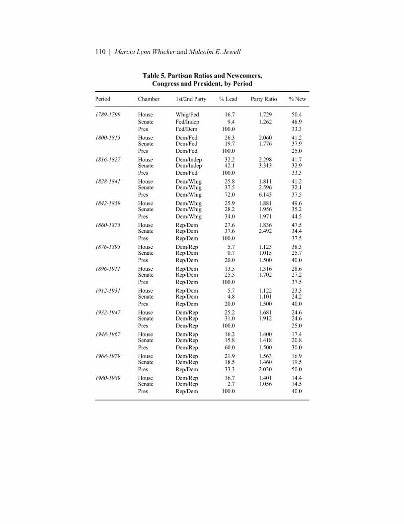
110 | Marcia Lynn Whicker and Malcolm E. Jewell
Table 5. Partisan Ratios and Newcomers, Congress and President, by Period
Period Chamber 1st/2nd Party % Lead Party Ratio % New 1789-1799 House Whig/Fed 16.7 1.729 50.4 Senate Fed/Indep 9.4 1.262 48.9 Pres Fed/Dem 100.0 33.3 1800-1815 House Dem/Fed 26.3 2.060 41.2 Senate Dem/Fed 19.7 1.776 37.9 Pres Dem/Fed 100.0 25.0 1816-1827 House Dem/Indep 32.2 2.298 41.7 Senate Dem/Indep 42.1 3.313 32.9 Pres Dem/Fed 100.0 33.3 1828-1841 House Dem/Whig 25.8 1.811 41.2 Senate Dem/Whig 37.5 2.596 32.1 Pres Dem/Whig 72.0 6.143 37.5 1842-1859 House Dem/Whig 25.9 1.881 49.6 Senate Dem/Whig 28.2 1.956 35.2 Pres Dem/Whig 34.0 1.971 44.5 1860-1875 House Rep/Dem 27.6 1.836 47.5 Senate Rep/Dem 37.6 2.492 34.4 Pres Rep/Dem 100.0 37.5 1876-1895 House Dem/Rep 5.7 1.123 38.3 Senate Rep/Dem 0.7 1.015 25.7 Pres Rep/Dem 20.0 1.500 40.0 1896-1911 House Rep/Dem 13.5 1.316 28.6 Senate Rep/Dem 25.5 1.702 27.2 Pres Rep/Dem 100.0 37.5 1912-1931 House Rep/Dem 5.7 1.122 23.3 Senate Rep/Dem 4.8 1.101 24.2 Pres Rep/Dem 20.0 1.500 40.0 1932-1947 House Dem/Rep 25.2 1.681 24.6 Senate Dem/Rep 31.0 1.912 24.6 Pres Dem/Rep 100.0 25.0 1948-1967 House Dem/Rep 16.2 1.400 17.4 Senate Dem/Rep 15.8 1.418 20.8 Pres Dem/Rep 60.0 1.500 30.0 1968-1979 House Dem/Rep 21.9 1.563 16.9 Senate Dem/Rep 18.5 1.460 19.5 Pres Rep/Dem 33.3 2.030 50.0 1980-1989 House Dem/Rep 16.7 1.401 14.4 Senate Dem/Rep 2.7 1.056 14.5 Pres Rep/Dem 100.0 40.0

Cohort, Turnover, and Partisan Effects in Elections | 111
of Republican to Democratic dominance drops from 1.702 to 1.500. The presidency goes from total Republican dominance during stability to a 20 percent lead during decay. The party dominance hypothesis also is supported by data from the 1932 election. The House ratio of Democratic to Republican support drops from 1.681 during stability to 1.400 during decay, while the equivalent Senate ratio drops from 1.912 to 1.418. The White House shifts from total Democratic dominance during stability to a 60 percent lead of Democrats over Republicans during decay. Finally, we might examine the increases in partisan ratios between each decay period and the subsequent critical election stability period, to find out if we are merely observing a long-term linear trend, or are seeing fluctua-tions that are tied the the rhythms of critical elections. If the fluctuations are tied to the rhythms of critical elections, we would expect dominant partisan ratios during stability periods to rise above their previous levels in decay periods, only to fall again in subsequent decay periods. The 1828-1841 stability period does not meet our expectations here, since the partisan dominance ratio for stability for the House is 1.811, lower than the partisan dominance ratio of 2.298 for the preceding decay period of 1816-1827. Similarly, the partisan ratio for stability for the Senate is 2.596, less than the partisan ratio of 3.313 for the preceding decay period. We note that the major party of comparison with the Democrats shifts across the two periods from Independents to Whigs. Had we used Whigs, not Independents, for the ratio for the preceding decay period, our expectations would have been met. Comparing the stability period of 1860-1875 with the preceding decay period of 1842-1859, our partisan dominance hypothesis expectations are met for the Senate and the presidency, but not for the House. Expectations are met for House, Senate and presidency alike when the 1896-1911 stability period is compared with the preceding decay period of 1876-1895. Similar-ly, expectations also are met when the stability period of 1932-1947 and the preceding decay period of 1912-1931 are compared for partisan dominance. With the exception, then, of the 1828 election (which is compounded by the shift in opposition from Independents to Whigs) and the House in the 1860 election, partisan ratio shifts are not tied to secular trends, but rather fluctuate rhythmically in synchronization with critical election cycles for the four critical elections identified by Clubb et. al. (1980). Dominant Party Percentages of Newcomers Versus Oldtimers in Different Periods. If the newcomer/turnover hypothesis of critical elections is supported, newcomers should have higher percentages of dominant party representation than oldtimers. According to the newcomer/turnover

112 | Marcia Lynn Whicker and Malcolm E. Jewell
hypothesis, the dominant party lead among newcomers (who provide fresh perspective and input), and not the overall party ratios, is the driving factor behind major policy shifts. The dominant party lead among newcomers should be greatest for critical election Congresses, and this gap should exceed that for mid-sequence adjustment Congresses and for the stability period. Dominant party leads among newcomers for stability periods should exceed the equivalent among decay periods. Table 6 presents data to examine these expectations. Table 6 provides only weak support for turnover effects. All compari-sons for 1828 are consistent with the newcomer/turnover hypothesis, but the 1860 period data are not supportive. Turnover expectations continue to be confounded in 1896, but are supported by midyear election results. In 1932, comparing the party affiliation of newcomers to oldtimers within the same time frame and Congresses provides only intermittent and weak support for the hypothesis that the partisan characteristics of newcomers, rather than total party ratios, drive policy shifts associated with critical elections.
Table 6. Comparison of Critical Year with Period, for Percentage of Newcomers and Oldtimers in Dominant Political Party
Newc Oldt Prob Newc Oldt Prob Year Pty Pty Diff ChSqa Period Pty Pty Diff Ch-Sqa
1789 42.1 � � � 1789-1799 39.4 39.8 0.4 .71 1800 50.0 34.3 -15.7 .13 1800-1815 48.3 53.1 4.8 .02*
1816 54.6 53.8 -0.8 .39 1816-1827 53.5 59.3 5.8 .00**
1828 69.7 62.4 -7.3 .03* 1828-1841 58.1 57.2 -0.9 .00**
1842 64.3 60.0 -4.3 .59 1842-1859 52.9 57.6 4.7 .00**
1860 56.7 54.4 -2.3 .05* 1860-1875 56.8 64.0 7.2 .00**
1876 59.0b 39.7b -19.3 .00* 1876-1895 48.1b 45.2b -2.9 .00**
1896 40.2b 67.6b 27.4 .00* 1896-1911 48.8b 59.2b 10.4 .00**
1912 66.0 64.5 -1.5 .10 1912-1931 53.6 52.3 -1.3 .08 1932 82.4 63.7 -18.7 .00** 1932-1947 60.4 62.8 2.4 .10 1948 65.6 57.4 -8.0 .00** 1948-1967 58.3 58.0 -0.4 .00**
1968 52.1 56.6 4.1 .71 1968-1979 58.4 61.3 2.9 .45 1980 29.4 60.0 30.6 .00** 1980-1989 49.3 58.6 9.3 .01**
aProbability of Chi-Square of political party versus newcomer/oldtimer. bRepublican percent *Chi-Square significant at .05 level. **Chi-Square significant at .01 level.
Cohort, Turnover, and Partisan Effects in Elections | 113
Background Characteristics of Newcomers versus Oldtimers in Differ-ent Periods. Relationships between the variable newcomer/oldtimer and six additional background variables, including political party affiliation, were tested but are not reported in detail here. The other five variables are age in 5-year categories, secondary education, college education, military service, level of prior government service before entering Congress, and whether or not a relative had served in Congress. A large number of statistically significant relationships showing that newcomers are different from oldtimers on a variety of background characteristics would support the cohort hypothesis of critical election policy change. However, very few statistically significant relationships were found for the critical election year Congresses of 1828, 1860, 1896, and 1932. Only in 1896 does a variable other political party or age attain statistical significance, and that same variable�prior government service�also is statistically significant in 1876, a non-critical mid-sequence adjustment Congress. The dearth of statistically significant relationships between newcomer/oldtimer and background characteristics undermines the cohort hypothesis. Summarizing the Four Critical Elections. Table 7 presents summary data for the four critical elections examined in depth here. Mean age differ-ences between the critical election Congresses and mid-sequence adjustment Congresses are miniscule (1.1 years average). Mean age differences between stability periods and decay periods are somewhat greater (1.8 years average), but only slightly more so. Neither observation provides strong support for the cohort hypothesis. Further, the gap for mean age between the initiating year and its subsequent period is greater overall for decay periods than for stability periods, undercutting the cohort hypothesis. Oldtimers are older than newcomers in decay periods and mid-sequence adjustment Congresses than in stability periods and critical election Congresses, further weakening the cohort hypothesis. Nor does the oldtimer/newcomer variable seem sig-nificantly related to many other background characteristics, except for poli-tical party and categorical age. These analyses, then, do not support the cohort notion that generational change drives basic policy shifts surrounding critical elections. Nor are the summary data supportive of the newcomer/turnover hy-pothesis. The average percentage of newcomers for critical election Con-gresses is 40.2 percent, only modestly above the average of 37.9 percent for mid-sequence adjustment Congresses. The percentage of newcomers for sta-bility periods is 35.5 percent, or 2.9 percent greater than the 32.6 percent newcomers averaged for decay periods. This finding is supportive of the turnover hypothesis, but only weakly so in the face of little or no difference

114 | Marcia Lynn Whicker and Malcolm E. Jewell
Table 7. Summary of Differences Between Periods Stability and Decay for 1828-1967
Stability Decay Differencea
Mean Age, Critical Year 48.8 49.9 1.1 Mean Age, Period 49.2 51.0 1.8 Mean Age Difference, Critical Yr and Period 0.525 1.225 0.700 Old v. New, Year 3.7 4.9 1.2 Old v. New, Period 4.0 5.2 1.2 % Newcomers Total, Year 40.2 37.9 -2.3 % Newcomers Total, Period 35.5 32.6 -2.9 % Newcomers Total, Diff. Yr-Period 4.75 5.7 1.0 % Newcomers, House 35.5 30.8 -4.7 % Newcomers, Senate 29.6 25.4 -4.2 % Newcomers, President 34.4 36.7 2.3 % Party Lead, House 23.0 13.3 -9.7 % Party Lead, Senate 32.9 12.2 -20.7 % Party Lead, President 93.0 34.1 -58.9 Party Ratio, House 1.661 1.373 -0.288 Party Ratio, Senate 2.176 1.357 -0.819 Party Ratio, President 6.143 1.725 -4.418 Dominant Pty % Diff. Old v. New, Year -0.2 -12.6 -12.4 Old v. New, Period 4.8 -1.7 -6.5 % Time Sig <= .05, For Newcomer/Oldtimer v. Political Pty, Year 100.0 100.0 0.0 Political Pty, Period 75.0 75.0 0.0 Age By 5-Yr Cat., Year 100.0 100.0 0.0 Age By 5-Yr Cat., Period 100.0 100.0 0.0 aDifference = Decay - Stability

Cohort, Turnover, and Partisan Effects in Elections | 115
between the percentages of newcomers for critical election Congresses and for mid-sequence adjustment Congresses. When averaging and comparing the percentages of oldtimers and new-comers in the dominant party during periods of stability, oldtimers have only 0.2 percent fewer members in the dominant party. Thus, oldtimers and newcomers are virtually equal in number in the dominant party during periods of stability. The turnover hypothesis would hold the contrary�that newcomers should average a higher share of the dominant party than do old-timers during such periods. A similar comparison of the distribution of oldtimers and newcomers in the dominant party for the decay period indi-cates that oldtimers comprise an average 12.6 percent smaller share of the dominant party; yet, the turnover hypothesis would support the reverse�that oldtimers are equal to or more numerous in the dominant party than new-comers during decay. These observations collectively provide little support for the turnover hypothesis. Examining average party ratios for periods of stability and decay, how-ever, reveals support for the partisan dominance hypothesis of policy shifts following critical elections. For the House, the Senate, and the presidency, the dominant party ratio for the stability period far exceeds the dominant party ratio for the decay period, as expected. The percentage of seats belonging to the dominant party during periods of stability also far exceeds the dominant party�s lead during the decay periods.
Conclusion These analyses support the notion that party power matters as a driving force behind major shifts in national policy surrounding critical elections. Various types of evidence also were examined pertaining to the alternative hypotheses that national policy shifts are produced by high turnover and an influx of newcomers to Congress, or by a cohort/generational effect. The data examined provided weak or no support for either of these alternative hypotheses. Some shifts in the data�especially the increase in mean age as decay replaces stability, and the decrease in turnover as stability gives way to decay�result from long term trends independent of critical election rhythms. In contrast, changes in party ratios were tied directly and strongly to critical election rhythms. Party differences in strength and platform may be the factor that influences national policy shifts. Thus, if �the party is over,� as David Broder has declared, voter choice and the capacity to respond to major national crises with dramatic policy shifts may be gone as well.
116 | Marcia Lynn Whicker and Malcolm E. Jewell
REFERENCES Alesina, Alberto. 1988. Credibility and Policy Convergence in a Two-Party System with Rational
Voters. American Economic Review 78: 796-806. ___________ and Howard Rosenthal. 1989. Partisan Cycles in Congressional Elections and the
Macroeconomy. American Political Science Review 83: 373-398. Alesina, Alberto and Jeffrey Sachs. 1988. Political Parties and the Business Cycle in the United
States, 1948-1984. Journal of Money, Credit, and Banking 20: 63-82. Baker, Ross K. 1989. The Congressional Elections. In Gerald M. Pomper, ed., The Election of 1988.
Chatham, NJ: Chatham House Publishers. Barber, James David. 1980. The Pulse of Politics. New York: W.W. Norton & Co. Beck, Paul Allen. 1979. The Electoral Cycle and Patterns of American Politics. British Journal of
Political Science 9: 129-156. Brady, David W. 1988. Critical Elections and Congressional Policy Making. Stanford, CA: Stanford
University Press. Burnham, Walter D. 1970. Critical Elections and the Mainsprings of American Politics. New York:
W.W. Norton. Ceaser, James W. 1979. Presidential Selection. Princeton, NJ: Princeton University Press. Chappell, Henry W. and William R. Keech. 1985. A New View of Political Accountability for
Economic Performance. American Political Science Review 79: 10-27. Clubb, Jerome M., William H. Flanigan, and Nancy H. Zingale. 1980. Partisan Realignment: Voters,
Parties, and Government in American History. Beverly Hills, CA: Sage Publishers. Crittenden, John A. 1982. Parties and Elections in the United States. Englewood Cliffs, NJ:
Prentice-Hall, Inc. Diamond, Robert A., ed. 1976. Origins and Developments of Congress. Washington, DC: Congres-
sional Quarterly Press. Dodd, Lawrence C. and Bruce I. Oppenheimer. 1985. The Elusive Congressional Mandate: The
1984 Election and Its Aftermath. In Lawrence C. Dodd and Bruce I. Oppenheimer, eds., Congress Reconsidered. Washington, DC: Congressional Quarterly Press.
Erikson, Robert S. 1971. The Advantage of Incumbency in Congressional Elections. Polity 3: 395-405.
__________. 1972. Malapportionment, Gerrymandering, and Party Fortunes in Congressional Elec-tions. American Political Science Review 66: 1234-1335.
Ferejohn, John A. 1977. On the Decline of Competition in Congressional Elections. American Politi-cal Science Review 71: 166-176.
Fiorina, Morris P., David W. Rohde and Peter Wissel. 1975. Historical Change in House Turnover. In Norman J. Ornstein, ed., Congress in Change. New York: Praeger Publishers.
Frantzich, Stephen E. 1989. Political Parties in the Technological Age. New York: Longman. Heard, Alexander and Michael Nelson. 1987. Change and Stability in Choosing Presidents. In Alex-
ander Heard and Michael Nelson, eds., Presidential Selection. Durham, NC: Duke University Press.
Hibbs, Douglas. 1977. Political Parties and Macroeconomic Policy. American Political Science Review 71: 1467-1487.
Hinckley, Barbara. 1981. Congressional Elections. Washington, DC: Congressional Quarterly Press. __________. 1978. Stability and Change in Congress. New York: Harper and Row. Hirschman, A. O. 1982. Shifting Involvements: Private Interest and Public Action. Princeton, NJ:
Princeton University Press. Jacobson, Gary C. 1987. The Politics of Congressional Elections, 2nd Ed. Boston, MA: Little,
Brown and Co. Key, V.O. 1966. The Responsible Electorate. Cambridge, MA: Harvard University Press. Kiewiet, D. Roderick. 1981. Policy-oriented Voting in Response to Economic Issues. American
Political Science Review 75: 459-488.

Cohort, Turnover, and Partisan Effects in Elections | 117
Kinder, Donald R. and D. Roderick Kiewiet. 1979. Economic Discontent and Political Behavior: The Role of Personal Grievances and Collective Economic Judgments in Congressional Voting. American Journal of Political Science 23: 495-527.
King, Michael E. and Lester G. Seligman. 1976. Critical Elections, Congressional Recruitment, and Public Policy. In Heinz Eulau and M.M Czudnowski, eds., Elite Recruitment in Democratic Politics: Comparative Studies Across Nations. New York: Halstead Press.
Kingdon, John W. 1973. Congressmen�s Voting Decisions. New York: Harper and Row. Kostroski, Warren Lee. 1973. Party and Incumbency in Postwar Senate Elections. American Poli-
tical Science Review 67: 1213-1234. Kramer, Gerald. 1983. The Ecological Fallacy Revisited: Aggregate Versus Individual-level Find-
ings on Economics and Elections and Sociotropic Voting. American Political Science Review 77: 92-111.
MacKuen, Michael B., Robert S. Erikson, and James A. Stimson. 1989. Macropartisanship. Ameri-can Political Science Review 83: 1125-1142.
Mann, Thomas E. and Raymond E. Wolfinger. 1980. Candidates and Parties in Congressional Elec-tions. American Political Science Review 74: 617-632.
Mayhew, David R. 1974a. Congressional Elections: The Case of the Vanishing Marginals. Polity 6: 295-317.
__________. 1974b. Congress: The ELectoral Connection. New Haven, CT: Yale University Press. __________. 1986. Placing Parties in American Politics. Princeton, NJ: Princeton University Press. McClosky, Herbert and John Zaller. 1984. The American Ethos. Cambridge, MA: Harvard Univer-
sity Press. Nexon, David H. 1980. Methodological Issues in the Study of Realignment. In Bruce A. Campbell
and Richard J. Trilling, eds., Realignment in American Politics. Austin: University of Texas Press.
Ornstein, Norman J., Thomas E. Mann, and Michael J. Malbin. 1987. Vital Statistics on Congress, 1987-1988. Washington, DC: Congressional Quarterly.
Pomper, Gerald M. 1967. Classification of Presidential Elections. Journal of Politics 29: 535-566. __________. 1977. The Decline of Partisan Politics. Political Science Quarterly 92: 23-41. Price, H. Douglas. 1971. The Congressional Career�Then and Now. In Nelson Polsby, ed., Congres-
sional Behavior. New York: Random House. Sabato, Larry J. 1985. PAC Power. New York: W.W. Norton and Co. Schlesinger, Arthur M. 1949. Paths to the Present. New York: MacMillan. Schlesinger, Jr., Arthur M. 1986. The Cycles of American History. Boston, MA: Houghton Mifflin
Co. Seligman, Lester G., and Michael R. King. 1980. Political Realignments and Recruitment to the U.S.
Congress, 1870-1970. In Bruce A. Campbell and Richard J. Trilling, eds., Realignment in American Politics. Austin: University of Texas Press.
Tufte, Edward R. 1973. The Relationship Between Seats and Votes in Two-Party Systems. American Political Science Review 67: 540-554.

118 | Marcia Lynn Whicker and Malcolm E. Jewell