co{evolutionary approach to the manpower planning …

CO–EVOLUTIONARY APPROACH TOTHE MANPOWER PLANNING

PROBLEM

Robert Michael Jacquier

A dissertation submitted to the Faculty of Science, University of theWitwatersrand, in fulfilment of the requirements for the degree ofMaster of Science

Johannesburg, 2010

brought to you by COREView metadata, citation and similar papers at core.ac.uk

provided by Wits Institutional Repository on DSPACE

https://core.ac.uk/display/39667999?utm_source=pdf&utm_medium=banner&utm_campaign=pdf-decoration-v1

Abstract. This dissertation will investigate a realistically sized manpower

planning problem. To perform the analysis, an appropriate model will be pre-

sented to solve a specific type of manpower problem. It allows for recruitment,

dismissal, training of workers to different types, and multi–skilled workers. The

training is enforced in the model through time delay. The model also includes

consistency, demand and bound constraints that the solutions must satisfy.

The solution of the model will then be investigated using a novel approach,

the competitive co–evolutionary algorithm. The algorithm generates solutions

in the same way a genetic algorithm does, and implements a predator–prey

procedure to ensure satisfaction of the constraints. A numerical example will

then be solved to illustrate the usefulness of the co–evolutionary algorithm

when applied to this type of manpower problem.

iii

I declare that this dissertation is my own, unaided work. It is being submitted for

the Degree of Master of Science in the University of the Witwatersrand, Johannes-

burg. It has not been submitted before for any degree or examination in any other

University.

(Signature of candidate)

day of

Contents

List of Figures ix

List of Tables xi

xv

Notation xv

Chapter 1. Introduction 1

1. The manpower planning problem 1

2. Co–evolutionary algorithms 6

Chapter 2. Overview of the model 9

1. The objective function 14

2. Model dynamics 14

3. Model constraints 14

Chapter 3. Analysis of the model 17

1. The optimisation problem 17

2. The objective function 17

3. Model dynamics 18

4. Model constraints 18

5. Problem size 20

Chapter 4. Analysis of the problem 23

1. Exponential growth 23

2. Optima in continuous and discrete systems 25

3. Constraint satisfaction problems 27

4. Computational complexity 28

5. Complexity classes 28

6. Non–linear integer programming problem 30

7. Branch and Bound 31

8. Dynamic programming 32

9. Optimal control approach 32

10. Modified genetic algorithm approach 33

v

vi CONTENTS

Chapter 5. Sensitivity analysis 37

1. Overview 37

2. Sensitivity of the bound constraints 38

3. Sensitivity of the fulfilment constraints 38

4. Sensitivity of the assignment consistency constraints 39

5. The perturbation of a constraint 39

6. Uncertainty of the demand parameters 40

7. Probability distribution for the demand parameters 41

8. Defining the measure of feasibility 41

Chapter 6. Refining the model 45

1. Constraint relaxation 45

2. Separability of the employment and assignment aspects 47

3. The power of multiple populations 49

4. Objective function minimisation versus feasibility, resource usage 52

Chapter 7. The algorithm 55

1. Overview of the algorithm 55

2. Implementation 57

3. Programming concepts 58

Chapter 8. Test cases 65

1. Test case 1 65

2. Test case 1 - Brute force algorithm results 67

3. Test case 1 - Co–evolutionary algorithm results 68

4. Test case 2 69



7. Test case 3 74



Chapter 9. Main problem 81

1. Main problem 81

2. Optimal solution results 84

3. Co–evolutionary algorithm results 88

Chapter 10. Conclusion 95

Appendix A. Calculations 97

1. Initial conditions for training 97

2. Maximum cardinality of the sets L(i) and M(i) 98

CONTENTS vii

Appendix. Bibliography 101

List of Figures

4.1 Number of variables versus number of solutions 25

4.2 Branch and bound tree 30

6.1 Overall solution space 50

6.2 Employment solution space 51

6.3 Assignment solution space 51

7.1 Detailed chromosome inheritance 60

7.2 Co–evolutionary algorithm collaboration graph 61

7.3 Chromosome inheritance 61

7.4 Constraint inheritance 62

ix

List of Tables

4.1 Number of variables versus number of solutions 25

4.2 Problem summary 35

4.3 Modified genetic algorithm initial solution feasibility 36

8.1 Test case 1 - General information 65

8.2 Test case 1 - General parameters 65

8.3 Test case 1 - Task information 65

8.4 Test case 1 - Hiring bounds 66

8.5 Test case 1 - Dismissal bounds 66

8.6 Test case 1 - Demand 66

8.7 Test case 1 - Hiring costs 66

8.8 Test case 1 - Dismissal costs 66

8.9 Test case 1 - Salaries 66

8.10Test case 1 - Initial workers 66

8.11Test case 1 - Optimal solution 67

8.12Test case 1 - Co–evolutionary Optimal solution 68

8.13Test case 2 - General information 69

8.14Test case 2 - General parameters 69

8.15Test case 2 - Task information 69

8.16Test case 2 - Hiring bounds 69

8.17Test case 2 - Dismissal bounds 70

8.18Test case 2 - Demand 70

8.19Test case 2 - Hiring costs 70

8.20Test case 2 - Dismissal costs 70

8.21Test case 2 - Salaries 70



xi

xii LIST OF TABLES


8.25Test case 3 - General information 74

8.26Test case 3 - General parameters 74

8.27Test case 3 - Tasks 74

8.28Test case 3 - Training information 74

8.29Test case 3 - Hiring bounds 75

8.30Test case 3 - Dismissal bounds 75

8.31Test case 3 - Training bounds 75

8.32Test case 3 - Training times 75

8.33Test case 3 - Demand 75

8.34Test case 3 - Hiring costs 75

8.35Test case 3 - Dismissal costs 75

8.36Test case 3 - Training costs 75

8.37Test case 3 - Salaries 75


8.39Test case 3 - Initial workers in training 76



9.1 Main problem - General information 81

9.2 Main problem - General parameters 81

9.3 Main problem - Task information 81

9.4 Main problem - Training information 82

9.5 Main problem - Hiring bounds 82

9.6 Main problem - Dismissal bounds 82

9.7 Main problem - Training bounds 82

9.8 Main problem - Demand 82

9.9 Main problem - Hiring costs 82

9.10Main problem - Dismissal costs 82

9.11Main problem - Salaries 83

9.12Main problem - Training costs 83

9.13Main problem - Training times 83

9.14Main problem - Initial workers 83

LIST OF TABLES xiii

9.15Main problem - Initial workers in training 83

9.16Main problem optimal solution - hiring variables 84

9.17Optimal solution - dismissal variables 85

9.18Optimal solution - training variables 86

9.19Optimal solution - assignment variables 87

9.20Main problem co–evolutionary solution - hiring variables 88

9.21Main problem co–evolutionary solution - dismissal variables 89

9.22Main problem co–evolutionary solution - training variables 90

9.23Main problem co–evolutionary solution - assignment variables 91

9.24Main problem co–evolutionary solution - available workers 92

9.25Main problem co–evolutionary solution - available workers 93

Notation

ZN+ The set of all positive integers, including zero

card(S) The cardinality of the set S

xv

CHAPTER 1

Introduction

1. The manpower planning problem

Manpower planning is a problem faced by an organisation that requires an em-

ployment policy that ensures that its demands for the future are met [1]. These

demands are often conflicting and solutions are difficult to find. These problems of-

ten consist of a large number of decisions that need to be made, making it necessary

to model the problem mathematically.

The usefulness and scope of manpower planning has increased over the decades,

given the increasing size and demands of organisations. Increased competition and

a general need to minimise cost has spurred growth in the areas of research linked

to manpower planning. Advances in various areas of mathematics have contributed

to the ability to deal with the manpower planning problem more effectively. Large

organisations, human resourcing departments and military departments consider

manpower planning one of their central concerns and have invested large amounts

of capital in dealing with the problem.

Manpower planning problems can be cast as optimisation problems [2]. These deal

with the employment policy, the assignment of workers to tasks, predicting the

future demand for manpower, and predicting the future supply for manpower. In

some cases the supply and demand forecasting problems are treated as inputs to a

more central problem: the employment policy and assignment of workers [3].

A paper by Edwards [2] surveyed the manpower planning models at the time. At

this time several facets of the problem had already been identified as being crucial.

These involve forecasting the demand for tasks in the future, forecasting the future

supply of manpower and adjusting the organisation’s policies to bridge the gap

between these two facets.

Today, data collection is widespread and there are many methods available for ac-

curately forecasting future demand. Simple methods for accomplishing this include

1

2 1. INTRODUCTION

extrapolation and regression. The variables representing the demand for tasks can

be stochastic or deterministic. A stochastic representation of these variables is

more natural given the nature of forecasting demand for the future, with the uncer-

tainty in demand increasing further into the future. Stochastic variables are usually

associated with some distribution which is defined by some average value and an

associated error. In the case of the normal distribution these are given by the mean

and variance respectively. As a first approximation, these stochastic variables can

be replaced by deterministic ones, with the demand values taking on some sort of

average measure of the stochastic variables. The measure of error can then be used

to simulate the true stochastic nature of the demand, as is done in Monte Carlo

simulations.

Assuming that the forecasting problem is solved, the manpower planning problem

can be split naturally into two remaining problems: the employment policy and

assignment. The employment policy problem deals with ensuring that sufficient

workers are available for assignment to the various tasks through the hiring, dis-

missal and training of workers while the cost of the process is minimised over a

period of time. The assignment problem then deals with assigning the available

workers to the various tasks.

The problems investigated are viewed at the macro level [1, 3, 4]. In this way they

only track the total number of a specific worker type and not specific individuals.

Models that track specific individuals would be examples of models that operate

at the micro level. The tendency to use macro models is mainly to ensure the

problem is still computationally tractable, but this approach has other benefits.

Often the computational solutions to the manpower problem are not meant to be

strict instructions of how an organisation should implement its employment policy,

but are meant to act as guidelines. Macro models can assist in providing these

guidelines by lumping workers into types, where these types are defined purely by

a set of shared characteristics. This enforces an ‘equality’ amongst workers of the

same type. Should an organisation require a micro view of its workers, the solution

of a macro level based problem can be used to identify individuals and implement

a preferred micro level solution.

Choosing an appropriate manpower planning model to represent the manpower

planning problem defines the problem mathematically. The properties of the man-

power problem suggest a certain natural structure. Quantities that are strictly

integers pervade the problem, in particular the number of workers hired, trained,

1. THE MANPOWER PLANNING PROBLEM 3

and dismissed. The decision variables and by implication the state variables are

therefore restricted to take on integer values.

The problem is generally formulated with a single objective function: the total cost

of the process over a finite time horizon. The objective is then to minimise this

cost, such that the constraints of the problem are met.

The manpower problem can involve optimising over one or more objective functions

subject to certain constraints, that may be non–linear. The employment policy sub–

problem involves recruitment, dismissal and training of workers and the assignment

sub–problem involves assigning the available workers to specific tasks that must be

performed. Both of these sub–problems must be addressed in such a way that the

constraints of the problem are satisfied.

Models invariably have their drawbacks, and manpower models are no exception.

Many models are formulated for extremely specific cases, with no possibility for

extending the models to other types of problems. This is often illustrated by the

assumptions the models make, such as homogeneous skill of the work force and

lack of training mechanisms. These restrict the applicability of the models. More

complex models rely on additional information: the ability to group workers and

tasks into types, the ability to codify training programs, knowledge of demand for

tasks in the future, and knowledge of restrictions on variables.

The size of the problem affects the solving of the model computationally. In reality,

manpower problems are large due to the number of decision and state variables

(which depend heavily on the planning horizon and number of workers in the prob-

lem). Some algorithms are developed exclusively for numerical examples which are

small compared to the problems faced in reality.

Over the years several approaches to solving the manpower planning problem (or

one of its sub–problems) have been introduced. Many use models that have some

common properties while others deviate in drastic ways to solve very particular

types of manpower planning problems.

Grinold [5] presents a manpower planning model that includes uncertain require-

ments for future demand. Finite Markov chains are used to represent the demand

for manpower at each time step in the model. The objective functions chosen are

based on minimising the expected value of a function of the difference between the

supply and demand for manpower. The objective functions used in the problem

are chosen to be quadratic for two reasons: they render the model solvable and

4 1. INTRODUCTION

are also a reasonable measure of the systems actual performance versus its ideal

performance. Time delayed training is modelled and continuation rates are used to

represent the retention, promotion and retirement of workers in the system.

Poornachandra Rao [6] follows a dynamic programming approach to the manpower

problem, seeking to minimise the total cost of the process. The model used is

analogous to the Wagner-Whitten model in inventory management. He critically

identifies recruitment, over–staffing, under–staffing, dismissal, recruitment and re-

tention costs for use in the model. The model is limited in that it is isolated from

the relevant organisations operating policies and the constraints that affect the

manpower problem.

Cai and Li [4] make use of a genetic algorithm for solving the manpower prob-

lem. The model introduced allows for mixed skilled workers and does not allow for

training of workers. Multiple objective functions are specified and integrated into

the genetic algorithm to perform the various evolutionary operations. The primary

objective is to minimise the total cost of the process, the secondary objective is

to maximise the surplus of staff when assigning costs are approximately the same,

and the tertiary objective is to reduce the variation of staff surplus over the time

periods in the model. The genetic algorithm then uses all of these objectives to

select breeders, and a multi–point crossover based on the Hamming distance be-

tween schedules is used to perform the crossover. A heuristic is used to reduce

the infeasibility created during crossover. Cai and Li [4] noted that it is extremely

important to find feasible regions before running the genetic algorithm and that

large planning horizons would require alternative algorithms to solve the problem.

Zanakis and Maret [1] introduced a Markovian goal programming approach to the

manpower problem, making use of a Markov type model based on historical prob-

abilities. The model allows for hiring, dismissal, retirements and other stochastic

processes. Guidelines specific to an instance of the problem are used to formulate

a linear goal programming model. The objective function used is to minimise the

overall cost of the process, and the model was solved for a single time step.

Brusco and Jacobs [7] used a simulated annealing approach to solve a scheduling

problem. The problem is basically a shift assignment problem where the objective

is to minimise the number of full time employees while satisfying the demand that

is forecast. The model makes use of bounds in the problem, and does not consider

constraints affecting the manpower problem.

1. THE MANPOWER PLANNING PROBLEM 5

Narasimhan [8] presented a custom algorithm to solve the assignment problem. The

model proposed introduces various constraints on the system. A hierarchical model

is used for workers to perform tasks, and the model does not allow for training of

workers. While the algorithm is only applicable to the type of problem described, it

has the desirable property where the computational time of the algorithm increases

linearly with the problem size.

Lee, Cai and Teo [3] presented the manpower problem as a time delayed optimal

control problem in discrete time. The model used allows for multi–skilled workers,

time delayed training, hiring, dismissal and assignment of workers. The objective

is to minimise the overall cost of the process. The problem initially consists of

integer decision variables and is transformed into a discrete valued optimal control

problem. Another transform is then used to reduce this problem to a standard

optimisation problem involving continuous variables, allowing it to be solved by

standard optimisation techniques.

Gass [9] gives an overview of military manpower planning models, highlighting

Markov models, network–flow models and multi–year models. The network–flow

models are powerful descriptive tools in that they do not require equations of state

to display the transform of flows. These models however, break down when time

dependent problems are considered. The multi–year models solve this shortcoming

by transforming a previous time steps’ workers.

The manpower model used in this paper is cast as a non–linear global optimisation

problem with non–linear constraints and a single objective function. While very

good global optimisation algorithms exist for particular problems, there are few

that can handle constraints without additional assumptions. Those that do include

penalty methods and heuristic methods. The penalty methods require other sub-

problems be solved, and are not completely reliable [10]. The heuristic methods

are used to alter infeasible solutions via some procedure, until they are feasible [4].

The problem of solving a manpower model is thus reduced to the task of finding an

appropriate model, and a global optimisation algorithm capable of handling non–

linear constraints. The dissertation will deal with the optimal employment policy

and assignment of workers to tasks at a macro level. The problem will be cast

as a non–linear integer programming problem with a single objective function, the

overall cost of the process. The goal is to minimise the cost of the process and

satisfy the constraints of the problem. All variables in the model are deterministic.

The demand is assumed to be some maximum value of the expected demand, or an

average value of the stochastic demand.

6 1. INTRODUCTION

2. Co–evolutionary algorithms

There are a variety of ways in which one can apply global optimisation algorithms

to handle constraints, yet the approaches yield mixed results depending on which

problems they are applied to [11].

A common and easily implementable approach is to make use of exterior penalty

methods. This approach introduces an auxiliary function with parameters that

is added to the objective function, as shown by Luenberger in [12] and Soleimani-

damaneh in [13]. The auxiliary function is chosen so as to penalise a solution heavily

for not satisfying the constraints, while leaving the objective function unchanged

for feasible solutions. There are several problems with this approach. The first is

that the distortion of the objective function assumes some measure of feasibility

of a solution, using this to make solutions gradually ‘more feasible’. The second

is that parameters introduced into the objective function must either be assumed

or solved for as part of another optimisation problem. An example is given in

[10], which describes a genetic algorithm that relies on penalty methods. This

approach illustrates how the distortion of the objective function does not always

yield satisfactory results.

Another approach to deal with the constraints is by using exterior point methods.

These methods generate solutions that are not guaranteed to be feasible, and make

use of the infeasible solutions that have been generated to generate solutions that

are feasible. This process is often gradual, as the set of initial solutions must be

combined to produce new solutions that are still not feasible. Some measure of

feasibility is then used to gradually generate solutions that lie inside the feasible

regions.

A naive way to implement a genetic algorithm to solve a problem with constraints

is to reject the infeasible solutions at each iteration. This approach severely limits

the size of the solution population in some problems. This approach may result in

a solution population with an extremely low number of feasible candidates, if any

at all. This is especially severe in problems where the ratio of feasible solutions

to the total number of solutions in the problem domain is small. Problems of this

nature tread a fine line between optimisation problems and satisfiability problems.

Exterior point methods are more reliable in dealing with problems such as these,

since they do not rely on solutions being feasible initially. In the context of the

genetic algorithm, there is a need for diversity in the population of initial solutions,

as well as subsequent generations. Solutions that are not initially feasible may

2. CO–EVOLUTIONARY ALGORITHMS 7

evolve to yield candidates that are more fit, and additional evolutionary operations

may result in feasibility.

Co–evolutionary algorithms represent a class of new algorithms that have shown

promise in global optimisation. They attempt to simulate the relationship between

multiple species that interact with each other and adapt as a result of these inter-

actions [14]. These include co–operative algorithms and competitive algorithms.

Co–operative co–evolutionary algorithms split the problem domain into sub–domains

and breed species that form partial solutions to the problem. A merging of individ-

uals from the various species then forms a complete solution to the problem. The

separate evolution of these species can be linked to the varying of a single variable

while all other variables are held constant. The separability of the variables in the

objective function underlies this approach.

The competitive algorithms rely on evolving two types of populations, predators

and prey. These populations evolve in such a manner that one is always trying

to outdo the other. These dynamics can result in what is termed an arms race in

the literature [15]. In this type of algorithm, the fitness of a species does not only

depend on the individual’s fitness, but also on the way it interacts with members

of the other species [16].

The underlying mechanisms for co–evolutionary algorithms are not well understood.

The beginnings of some progress in this area have been made by using a dynamical

systems approach to study the effects of various processes on the ways in which the

algorithms behave.

Westra and Paredis [15] used a co–evolutionary genetic algorithm to solve a path

planning problem in two dimensional space with static obstacles. This made use of

one population of goal seeking agents and another population of difficult starting

points. It was found that the co–evolutionary genetic algorithm outperformed a

normal genetic algorithm due to its ability to move out of local minima.

Potter and De Jong [17] introduced a general model for implementing the co–

evolution of co–operating species. This was done by creating several sub–populations,

each of which consisted of members that only represented a sub component of the

complete solution. These sub–populations evolve separately and form fit, complete

solutions. A critical finding was that the co–evolutionary algorithm performed

worse on problems with interacting variables than a traditional genetic algorithm.

8 1. INTRODUCTION

In [18], Popovici and De Jong investigated the cooperative co–evolutionary dy-

namics via fitness landscapes. A dynamical systems approach was used to analyse

patterns that could lead to performance gains for the algorithm. The investigation

found that the size of the population chosen and implementations of elitism affect

the algorithm’s performance in non–trivial ways.

Jansen and Wieg [19] provided evidence that the separability of the objective func-

tion in a problem is not the only property required to make a co–operative co–

evolutionary algorithm beneficial. They noted that the explorative capabilities of

such an algorithm are also an important factor. It was found that the expected

frequency of mutation in a co–operative co–evolutionary algorithm is higher than

a traditional evolutionary algorithm, and is the cause of this increased explorative

capability.

Wiegand, Liles and De Jong [20] performed an empirical analysis of collaborative

methods in cooperative co–evolutionary algorithms. The focus was on how the algo-

rithm select collaborators for evaluation. It was concluded that for static objective

functions, an optimistic approach on collaboration is best.

Iorio and Li [21] focused on the application of the cooperative co–evolutionary

algorithm to multi–objective problems. A method of non–dominated sorting was

used to reward successful collaborations. It was found that the algorithm was

successful due to the fact that it acquired a large number of diverse, non–dominated

solutions.

This dissertation will use a co–evolutionary algorithm to solve a manpower planning

model. The competitive co–evolutionary algorithm will model the solutions as

prey and the constraints of the problem as predators. These populations will then

interact in the same way as they would in a traditional predator–prey model.

CHAPTER 2

Overview of the model

This chapter presents the essentials of the manpower planning model used. Details

and consequences of the model are discussed in following chapters.

The manpower problem considered will consist of the the employment and assign-

ment sub–problems.

We model the manpower planning problem at the macro level by introducing the

concept of a worker type. We assume the problem consists of N worker types. All

workers of a particular type are indistinguishable from one another.

For the employment problem, we need to ensure that the cost of the entire process

is minimised while satisfying the constraints of the problem. We are required to

make decisions such as the number of workers of a particular type to hire, dismiss

and train at various points in time. The intervals at which these decisions are made

can be assumed to be discrete, as there is normally a set interval in organisations to

perform these types of actions. For example, workers are often hired or dismissed

at the end of a month. Let t represent the current time step of the problem, where

t = 0, . . . , T and T represents the final time up to which we want to solve the

manpower problem. Our problem therefore consists of T + 1 time steps.

The characterisation above allows us to introduce employment variables for the

problem. Let hi(t) be the number of type i workers hired at time t, fi(t) be the

number of type i workers dismissed at time t and uij(t) be the number of type i

workers to be trained to type j at time t. These decision variables provide a basis

for expressing the decisions we make regarding our employment policy. With these

variables defined, some basic costs can be considered. Let chi (t) be the cost of hiring

a new worker of type i at time step t. Then the total hiring costs for worker type

i at that time step are

hi(t)chi (t).

9

10 2. OVERVIEW OF THE MODEL

Similarly, we can define the cost for dismissing a type i worker at time t as cfi (t).

The total dismissal costs for type i workers at that time step are

fi(t)cfi (t).

To implement training in the model, each worker type i has associated with it a set

of worker types L(i). Given i 6= j, the interpretation of this set is that a worker of

type i may be trained to a worker of type j if j ∈ L(i).

Let us define the cost for sending a type i worker for training to a type j at time t

as cuij(t). The total cost for training worker type i at time t must be summed over

all worker types that worker type i can be trained to. The total training costs for

worker type i at that time step are then∑j∈L(i)

uij(t)cuij(t).

These costs are a direct result of the decisions that are made. However, recurring

costs such as salaries and the maintenance of workers in training also need to be

taken into account. To account for these costs we introduce the following state

variables. Let xi(t) be the number of workers of type i at time t and let yij(t) be

the number of workers in training from worker type i to worker type j at time t.

These state variables allow us to quantify the costs associated with salaries and

maintaining workers in training. At each time step workers not in training are paid

their salaries, and workers in training are paid the salaries they were earning before

they entered training.

Let si(t) be the salary of a type i worker at time t. The total cost of salaries for

type i workers at time t is then

xi(t)si(t).

The total cost for maintaining a type i worker undergoing training to another worker

type at time t must be summed over all worker types that worker type i can be

trained to. The total training maintenance costs for all type i workers at that time

step are then ∑j∈L(i)

yij(t)si(t).

2. OVERVIEW OF THE MODEL 11

To calculate the cost of the entire process, we now need to sum the above costs

over all worker types, and over each time period. This leads to the following total

cost function

C =

T∑t=0

C(t),

where

C(t) =

N∑i=1

hi(t)chi (t) + fi(t)cfi (t) + xi(t)si(t) +

∑j∈L(i)

uij(t)cuij(t) +

∑j∈L(i)

yij(t)si(t)

.

Given our introduction of the state variables xi(t) and yij(t), we need to find

expressions for these in terms of our problems parameters and decision variables.

We will model the training in the model by removing the workers in training from

the pool of assignable workers and returning them to the pool after a period of time

equal to the duration of training. Let τij be the duration of training required to

train a type i worker to a type j worker. We impose the following restrictions on

the values of τij , given by

τij ≥ 1, τij ∈ Z+.

The state variables can be defined by specifying the flow of workers of a given type

from one time step to the next and specifying initial conditions. The number of

workers of worker type i at the next time step is affected by the current numbers

of workers xi(t), workers hired hi(t), dismissed fi(t), workers exiting for training∑j∈L(i) uij(t), and workers returning from training after the appropriate time delay∑j|i∈L(j) uji(t− τji). The set indicated by j|i ∈ L(j) should be interpreted as the

set of all worker types j that can be trained to type i. The number of workers at

time step t+ 1 is given by

xi(t+ 1) = xi(t) + hi(t)− fi(t)−∑j∈L(i)

uij(t) +∑

j|i∈L(j)

uji(t− τji).


Initially (t = 0), we assume there are a given number of workers of each type, given

by

xi(0) = ξi, i = 1, . . . , N.

The number of workers in training at the next time step is affected by the current

numbers of workers undergoing training yij(t), workers entering training uij(t), and

workers exiting training after the appropriate delay uij(t− τij). This is given by

yij(t+ 1) = yij(t) + uij(t)− uij(t− τij).

Initially (t = 0), we assume there are a certain number of workers in training,

yij(0) = χij , i = 1, . . . , N, j ∈ L(i).

Natural bounds for the hiring, dismissing, and training of workers are known. These

are either derived from business policy or physical limitations in the employment

environment. Bounds on hiring exist as a limitation on a maximum number of a

particular worker type that the organisation can afford. Let bhi (t) be the maximum

number of workers of type i that can be hired at time t. The hiring bound constraint

then takes the form

hi(t) ≤ bhi (t), i = 1, . . . , N.

Similarly, labour regulations may limit the number of workers that can be dismissed,

and limitations on training facilities may restrict the number of workers that can

be trained. These can similarly be cast in the form of bound constraints as

fi(t) ≤ bfi (t), i = 1, . . . , N,

uij(t) ≤ buij(t), i = 1, . . . , N, j ∈ L(i).

We now consider the assignment sub–problem. Each worker type i is capable of

performing a set of tasks M(i). The tasks form the basis for which demand must be

satisfied. Thus by assigning a sufficient number of workers to a task, the demand

2. OVERVIEW OF THE MODEL 13

for a task can be met. Let the demand for a task m at time t be given by dm(t). The

assignment decisions we are then required to make can be expressed by defining the

variables vim(t), the number of type i workers assigned to task m at time t. The

satisfaction of the demand requirement can then be expressed by the constraint∑i|m∈M(i)

vim(t) ≥ dm(t), m = 1, . . . ,M.

This ensures that demand is met or exceeded at every time step.

The parameters dm(t) are assumed to be inputs to the problem. This is effectively

a problem to forecast future demand for tasks, for which methods already exist.

A crucial link between the employment and assignment sub–problems is a consis-

tency requirement. At any particular time step, we are not permitted to assign

more workers to tasks than the number of workers the organisation actually pos-

sesses at that time. We thus need to ensure that at each time step, and for each

type of worker, the number workers assigned to all possible tasks does not exceed

the number of workers available. This translates into the following consistency

constraints ∑m∈M(i)

vim(t) ≤ xi(t), i = 1, . . . , N.

Since any employment decisions that are made at the final time step can only

increase the cost of the process without satisfying any constraints, we impose the

condition that we may not hire, dismiss or train any workers at the final time step

T , as given by

hi(T ) = fi(T ) = uij(T ) = 0, i = 1, . . . , N, j ∈ L(i).


1. The objective function

We cast the manpower planning problem as an optimisation problem. We seek to

minimise the overall cost of the process, that is given by

(1.1) minC =

T∑t=0

C(t)

where

C(t) =

N∑i=1

[hi(t)chi (t) + fi(t)c

fi (t) + xi(t)si(t)

+∑j∈L(i)

uij(t)cuij(t) +

∑j∈L(i)

yij(t)si(t)].

(1.2)

2. Model dynamics

The evolution of the system is governed by the balance equations


uij(t) +∑

j|i∈L(j)

uji(t− τji),(2.1)

yij(t+ 1) = yij(t) + uij(t)− uij(t− τij).(2.2)

Supplemented by the initial conditions

xi(0) = ξi, i = 1, . . . , N,(2.3)

yij(0) = χij , i = 1, . . . , N, j ∈ L(i).(2.4)

As well as the enforcement of the final conditions

hi(T ) = fi(T ) = uij(T ) = 0, i = 1, . . . , N, j ∈ L(i).(2.5)

3. Model constraints

The constraints for the system are of three types: demand, consistency and bound

constraints.

The demand constraints are given by∑i|m∈M(i)

vim(t) ≥ dm(t), m = 1, . . . ,M.

3. MODEL CONSTRAINTS 15

The worker assignment consistency constraints are given by∑m∈M(i)

vim(t) ≤ xi(t), i = 1, . . . , N.

The bound constraints for decision variables hi(t), fi(t), uij(t) are given by

hi(t) ≤ bhi (t), i = 1, . . . , N,

fi(t) ≤ bfi (t), i = 1, . . . , N,

uij(t) ≤ buij(t), i = 1, . . . , N, j = 1 ∈ L(i).

The control and state variables are constrained to take on positive integer values,

specifically

hi(t) ∈ ZN+ , i = 1, . . . , N, t = 0, . . . , T − 1,

fi(t) ∈ ZN+ , i = 1, . . . , N, t = 0, . . . , T − 1,

uij(t) ∈ ZN+ , i = 1, . . . , N, j ∈ L(i), t = 0, . . . , T − 1,

vim(t) ∈ ZN+ , i = 1, . . . , N, m ∈M(i), t = 0, . . . , T,

xi(t) ∈ ZN+ , i = 1, . . . , N, t = 1, . . . , T,

yij(t) ∈ ZN+ , i = 1, . . . , N, j ∈ L(i), t = 1, . . . , T.

CHAPTER 3

Analysis of the model

This chapter analyses the model presented in more detail. The objective func-

tion, balance equations and constraints are all studied and some of their properties

discussed.

1. The optimisation problem

We cast the manpower planning problem as an optimisation problem, minimising

the overall cost, C, given by (1.1).

2. The objective function

The objective function of the model is defined to be the total cost of the process.

The previous chapter showed how various costs, such as hiring, dismissal, training,

and maintenance costs make up the total cost, as given by (1.2)

The total cost of the process consists of costs from each time step, over the entire

planning horizon.

The objective function contains the decision variables hi(t), fi(t), uij(t) and the

state variables xi(t), yij(t). It should be noted that the objective function is linear

in the decision and state variables. The linearity of the objective function is thus

determined by whether the state variables are linear functions of the decision vari-

ables. In this model, the state functions are non–linear functions of the decision

variables due to time delay terms. This results in a non–linear objective function

for the problem.

17

18 3. ANALYSIS OF THE MODEL

3. Model dynamics

The model dynamics are given by the equations (2.1) and (2.2), the initial conditions

are given by the equations (2.3) and (2.3), and the final conditions are given by

equation (2.5).

The time delay term in the argument for the training is critical to tracking the

number of workers currently in training. The structure of the balance equations

ensures that the workers in training are not in the pool of assignable workers.

The time delay arguments also ensure that workers re–enter the pool of assignable

workers after the correct duration of training time. The state variables yij(t) are

thus only used as a mechanism for tracking the number of workers in training. The

time delay arguments introduce an element of non–linearity which, while making

the model more realistic, introduces complexities that are not easily to analyse. The

usual assumptions of linearity associated with the objective function and constraints

which involve the state variables are thus no longer valid.

The initial conditions set the number of workers of type i at time t = 0 equal to

ξi, and set the number of workers undergoing training from type i to type j at

time t = 0 to χij . For a case where χij 6= 0, additional information is required for

the problem to be well defined. The section Initial conditions for training in the

appendix provides a more detailed description.

The final conditions are imposed since the effect of employment variables at the

final time step T has no impact on the satisfaction on the demand constraints at

the final time step. This is since xi(T ) and yij(T ) are functions of control variables

of all previous time steps only.

The decision variables in the problem are hi(t), fi(t), uij(t) for all 0 ≤ t < T and

vim(t) for all 0 ≤ t ≤ T . Together with the initial conditions, these determine the

values of the variables xi(t) and yij(t) for all t, and thus the value of the objective

function. The satisfaction of the constraints is also determined by these variables.

4. Model constraints

4. MODEL CONSTRAINTS 19

The demand constraints∑i|m∈M(i)

vim(t) ≥ dm(t), m = 1, . . . ,M

require that a sufficient number of workers be assigned to perform a particular

task at a specific time step. Evaluation of the demand constraints only requires

knowledge of the demand and the required control variables vim(t). The evaluation

of this constraint is thus computationally cheap, since it is the comparison of a sum

of decision variables and a constant value.

The demand constraints are also used to set up the upper bounds for each of the

decision variables vim(t). This is done by setting the upper bound of each vim(t)

to the relevant demand constant, plus some percentage.

The worker assignment consistency constraints∑m∈M(i)

vim(t) ≤ xi(t), i = 1, . . . , N

require that a sufficient number of workers to perform a task are available for

assignment. For a particular worker type i, the total number of workers assigned

over all tasks m,∑m∈M(i) vim(t) cannot exceed the number of workers available

at that time, xi(t). Were this constraints not present, it would be possible to

assign workers that the organisation does not possess in sufficient numbers. These

constraints are functions of the assignment control variables and the state variables

xi(t). The constraints are thus non–linear and require computation of xi(t), which

is far more expensive to compute than the other constraints in the problem. The

state variables xi(t) become progressively more convoluted (with the contribution

of time delay terms) and more expensive to calculate as t increases. The constraints

for t = 0 are in fact linear, since xi(0) = ξi is a constant.

These constraints form the link between the assignment and employment aspects

of the problem. Due to the constraints being a function of the assignment and

employment variables, they are also the most difficult to satisfy.

The set indicated by i|m ∈M(i) should be interpreted as the set of all worker types

i that are capable of performing task m.

20 3. ANALYSIS OF THE MODEL

The bound constraints for decision variables hi(t), fi(t), uij(t), given by

hi(t) ≤ bhi (t), i = 1, . . . , N,

fi(t) ≤ bfi (t), i = 1, . . . , N,

and

uji(t) ≤ buij(t), i = 1, . . . , N, j = 1 ∈ L(i)

impose upper limits on the number of workers that may be hired, dismissed or

trained at time t, for each type of worker. As simple functions of the bounds and

control variables, these constraints are computationally cheap to compute.

Since the bound constraints are all linear and form bounding regions for the vari-

ables, they are used to specify the domain for each the employment variables. Due

to this fact, they are also trivially satisfied. They only need to be considered since

genetic operations might increase the value of a particular employment variable

outside of the range specified by these constraints.

The decision and state variables are constrained to take on positive integer values.

These restrictions are implicitly satisfied by using a particular integer parametrisa-

tion for the decision variables in the algorithm. The fact that the state variables are

functions of the decision variables, along with the consistency constraints ensures

that the state variables satisfy the integer constraints.

5. Problem size

Let card(S) represent the cardinality of the set S and let r represent the number

of tasks in the problem.

5. PROBLEM SIZE 21

The number of decision variables nd in the problem is

nd = (# Hiring variables) + (# Dismissal variables) + (# Training variables)

+ (# Assignment variables)

= (TN) + (TN) +

(T

N∑i=1

cardL(i)

)+ (T + 1)

(N∑i=1

cardM(i)

)

= (T )

(2N +

N∑i=1

cardL(i)

)+ (T + 1)

(N∑i=1

cardM(i)

).

The number of state variables ns in the problem is

ns = (# Workers of a type variables) + (# Workers in training variables)

= (TN) +

(T

N∑i=1

cardL(i)

)

= (T )

(N +

N∑i=1

cardL(i)

).

The number of constraints nc in the problem is

nc = (# Hiring constraints) + (# Dismissal constraints) + (# Training constraints)

+ (# Demand constraints) + (# Consistency constraints)

= (TN) + (TN) +

(T

N∑i=1

cardL(i)

)+ ((T + 1)r) + ((T + 1)N)

= (T + 1) (N + r) + (T )

(2N +

N∑i=1

cardL(i)

).

For example, a problem that consists of 10 worker types (N = 10), 15 tasks (r = 15),

taken over 12 time (T = 11) steps with∑Ni=1 cardL(i) = 10 and

∑Ni=1 cardM(i) =

15 gives

nd = 510,

ns = 220,

nc = 630.

CHAPTER 4

Analysis of the problem

This chapter gives brief overviews of topics that have an impact on the problem

under consideration. These include the exponential growth faced by problems of

this nature, the discrete nature of the problem, the complexity of the problem from

the view of computer science, and various methods of solving the problem.

1. Exponential growth

Exponential growth is a well known problem that results from the exponential

increase in size of a solution space when there is a linear increase in the number of

variables. Brute force algorithms check every solution in a solution space to find

the global optima, and are thus susceptible to this problem. Solving problems with

small numbers of variables using a brute force algorithm is tractable, but as soon

as the number of variables in the problem increase beyond a certain point, brute

force algorithms become an impractical method of solution.

Many algorithms that are widely in use exhibit exponential complexity in the worst

case. However, these algorithms are widely used because they perform better than

the worst case for many classes of problems they are used to solve. Even the

well known simplex method, renowned for its ability to solve large–scale, realistic

problems in less than exponential time, is known to have worst case exponential

complexity.

To illustrate the exponential growth of a problem, let lbi be the inclusive minimum

bound for variable i and let ubi be the inclusive maximum bound for variable i. The

total number of solutions ns in a search space of N variables is then given by

ns =

N∏i=1

(ubi − lbi + 1).

23

24 4. ANALYSIS OF THE PROBLEM

As an example, consider a problem with 10 variables, each of which can take on 10

possible values. The total number of solutions in the search space is given by

ns =

N∏i=1

(ubi − lbi + 1)

=

10∏i=1

(10)

= 1010.

Compare this with the number of variables in a problem which has only 10 more

variables than the original problem. The total number of solutions in this new

search space is given by

n′s =

N∏i=1

(ubi − lbi + 1)

=

20∏i=1

(10)

= 1020.

The result shows there is an increase of ten orders of magnitude between the sizes

of each search space, that was only brought on by doubling the number of variables

in the problem. Since even small problems generate a large solution space that

needs to be searched, larger problems result in search spaces which are practically

impossible to check using brute force algorithms. Heuristic algorithms are used to

sample the search space and use certain rules to improve on the initial solutions.

Figure 4.1 and Table 4.1 illustrate the relationship between the number of variables

and number of solutions when each of the variables added to the problem has 10

possible values.

2. OPTIMA IN CONTINUOUS AND DISCRETE SYSTEMS 25

Table 4.1. Number of variables versus number of solutions

Number of variables Number of solutions1 102 1004 100008 1× 108

16 1× 1016

32 1× 1032

64 1× 1064

128 1× 10128

256 1× 10256

Figure 4.1. Number of variables versus number of solutions

This example illustrates a fundamental problem with algorithms that exhibit worst

case exponential behaviour. Given the ability to compute the original problem, we

would need to have 1010 times more computing resources to solve a problem that

only has double the number of variables. Methods to circumvent this problem have

been and remain a major focus of modern computer science.

2. Optima in continuous and discrete systems

Discrete systems deal with variables whose values can take on, at most, a countably

infinite number of values. The countable nature of the values is a result of some

indivisible unit that is a characteristic of the set of numbers used to represent these


values. Together with an appropriate set of bounds on the variables and a particular

set of numbers, a discrete system can consist of variables that only take on a finite

number of values. This finite number of values may result in a solution space that

is impractical to check completely.

Continuous systems deal with variables whose values take on an uncountable range

of values. The uncountable nature of the range of values is a result of the inability

to order the set of values.

The concept of a local minimum in a continuous system can be defined. x′ is a

local minimum of f if

∃ ε > 0 st ∀x satisfying d(x, x′) ≤ ε

⇒ f(x′) ≤ f(x),

where d(x, x′) is a metric on the space.

If we further assume that f is strictly convex and there is a unique point x∗ such that

f ′(x∗) = 0, then the following two conditions are sufficient for a global optimum,

given a unique point x∗:

f ′(x∗) = 0

f ′′(x∗) > 0.

The calculus of continuous systems thus allows one to find the global minimum

using a straightforward procedure. Discrete systems hold no such advantage, as the

concept of convexity is not well defined. The only way to find a global minimum

is to check the objective function value of every candidate solution, and return the

optimal solution.

Algorithms to optimise an objective function typically generate an initial solution,

or a set of initial solutions. These are used in an iterative manner with a set of

rules to generate new solutions. The set of rules used fall into two major categories:

deterministic and heuristic.

Convex optimisation methods typically make use of the calculus of Newton and

Leibnitz, utilising gradient information about the problem. This can be used in

various ways by the algorithms to decide on how to move towards better solutions.

3. CONSTRAINT SATISFACTION PROBLEMS 27

This forms the basis for the convex optimisation methods such as the steepest

descent and conjugate gradient algorithms.

By contrast, algorithms that deal with discrete problems can assume no knowledge

of a gradient for the problem, since it is not well defined. The algorithm used still

requires some way to generate better solutions. Instead of using a deterministic

rule to calculate a path to move along, a heuristic rule is used. A process that

makes use of a solution’s objective function values is applied in conjunction with

the generation of random numbers to produce a set of decisions that should, on

average, generate better solutions.

3. Constraint satisfaction problems

Constraint satisfaction problems deal with a set of candidate solutions that must

satisfy a set of constraints. These problems deal with large solution spaces where

it is intractable to use brute force methods to solve the problem.

Consider the manpower model presented with a rigorous set of constraints. In a

practical sense, the problem moves away from being a pure optimisation problem to

a constraint satisfaction problem. The primary objective is then to find a solution

that satisfies the constraints of the problem, assuming such a solution exists.

Several methods are used to solve constraint satisfaction problems, one of which is

backtracking. Due to the large solution spaces involved, the methods must have

mechanisms to discard large areas of the search space (such as the pruning mecha-

nism used by branch and bound) while using a reasonable amount of resources.

The primary factor in deciding whether the manpower problem should be considered

as an optimisation problem or a constraint satisfaction problem is the ratio of the

total number of feasible solutions s to the total number of solutions n. The total

number of solutions is generally easy to compute given the range of each of the

variables in the problem, but calculating s would in general require evaluating

every constraint in the problem for each possible solution. This brute force method

would result in the solution to the problem, but is practically impossible given all

but the most trivial problems.

We thus consider a uniformly random sample of the solution space, of size nz. We

can then compute the number of feasible solutions in the sample, sz, and use this

to form an approximation of the ratio of feasible solutions to total solutions


s

n≈ sznz

s ≈ nsznz

.

In the limit of the sample size approaching infinity, the approximation becomes

exact

limnz→∞

sznz

=s

n.

This is an important step in deciding how to approach the problem, since the meth-

ods for dealing with optimisation problems and constraint satisfaction problems

have completely different goals.

4. Computational complexity

The study of complexity in computational terms is concerned with the amount of

resources required to solve a problem, assuming it is solvable. The resources that

are normally considered are storage and the time required to solve the problem.

The resources needed to solve a problem are dependent on the inputs of a problem.

Given that the amount of resources used to solve the problem is expressed as a

function of the inputs, the required resources for the problem can be calculated.

The primary resources considered are the time required to find a solution to a prob-

lem (associated with the time complexity of a problem) and the memory required

(associated with the space complexity of a problem). Thus, as the number of inputs

to a problem are changed, the resources required to solve the problem are affected

as well.

5. Complexity classes

A major area of research in Computer Science is to classify problems into complexity

classes. These classes represent problems with common characteristics in terms of

the ability we possess to test a candidate solution, and how many resources are

consumed in finding solutions to the problem.

5. COMPLEXITY CLASSES 29

A complexity class is a set of problems that are solvable by a model with certain

resources. These resources are traditionally expressed as functions of the inputs of

the problem.

The discussion of complexity classes and the solutions of problems using algorithms

are often described using a mathematical abstraction of a computer called a Turing

machine. This mathematical construct consists of a tape of infinite length, as well

as a ‘head’ that can read a bit from the current section of the tape, and write a

bit to the current section of the tape. The Turing machine also has a set of rules

that specify what data should be written and how the head should move (a unit

forwards or backwards), given the current state and data on the current section of

the tape.

Two useful types of Turing machines are used in complexity theory: deterministic

and non–deterministic. The deterministic Turing machine follows the definition

given above, while the definition for a non–deterministic Turing machine is modified

somewhat. A non–deterministic Turing machine calculates all possible transitions

from the current state in parallel, until a solution is reached. One interpretation

of this definition is that at every possible branch a new instance of a deterministic

Turing machine is spawned to compute the result of that specific branch.

The complexity class P is the set of all decision problems that are solvable in

polynomial time by a deterministic Turing machine. Thus, if x is the number of

inputs to the problem, a P class problem requires the following amount of resources

to solve

xa

for some constant a.

In practice, the constant a cannot be a large number for the problem to be practi-

cally solved.

The class NP is the set of decision problems that are solvable in non–deterministic

polynomial time by a non–deterministic Turing machine. A NP problem also has

the characteristic whereby a candidate solution can be checked to be a solution to

the problem in polynomial time. The Travelling Salesman problem and Boolean

Satisfiability problem are two examples of NP problems.


Figure 4.2. Branch and bound tree

It is well known that the non–linear integer program is a NP–Hard problem. This

class of problem is at least as hard as the hardest problem in NP. There is currently

no algorithm that is known to solve NP–Hard problems in polynomial time.

6. Non–linear integer programming problem

In general the Manpower problem can be expressed as

min C(A,B),

such that

fi = 0 i = 1, . . . , p,

gj ≥ 0 j = p+ 1, . . . , q,

where A and B are vectors of the decision and state variables respectively. The

functions fi and gj are functions of the decision and state variables.

This is the form of a non–linear integer programming problem. This general formu-

lation captures the familiar optimisation problems of constrained linear optimisa-

tion, unconstrained optimisation and other cases. This more general problem can

be solved by various methods, some of which are outlined below.

7. BRANCH AND BOUND 31

7. Branch and Bound

Branch and Bound is a global optimisation technique that is widely used. It ab-

stracts the problem into an implicit tree structure, minimising the need for storage.

The tree represents the solution space and the algorithm systematically searches

through this tree to find the optimal solution. A solution is represented by a

traversal from a node at the top of the tree to the bottom of the tree. Once a

parametrisation is chosen for how to map a solution into the tree structure, the

algorithm can use various rules to navigate the search space. Figure 4.2 shows

a special form of a tree structure, the binary tree, commonly used to represent

problems which can be parametrised by a binary structure.

Branch and bound can eliminate large areas of the solution space during a single step

if an appropriate parametrisation is chosen. It does so by selecting which part of the

tree to traverse next (branching), and then calculating upper and lower bounds for

the solutions that form a subset of the current node in the tree (bounding). The

bounds are then used to decide whether to proceed branching down the current

node, or whether the current section of the tree can be pruned. Pruning is a

process whereby all nodes below a particular node are removed from consideration,

since they are known to not contain the optimal solution. This process continues

until the entire tree has been pruned or one solution remains.

In the worst case, the algorithm will have to traverse the entire tree to find the opti-

mal solution, resulting in exponential time complexity. An appropriate parametri-

sation is required to try and avoid this. The other critical requirement is having

an efficient way of computing the bounds on the objective function for subsets of

solutions.

The manpower problem can utilise a modified branch and bound algorithm. The

bounding step can be modified so that in addition (or precluding) the objective

function bounds being calculated, the constraints in the problem are used to check

whether the tree can be pruned. Given the varying degree of constraints affecting

solutions in the manpower problem, the weaker constraints will be satisfied by most

solutions while the more restrictive constraints will result in large areas of the search

space being removed from consideration.


8. Dynamic programming

A method that effectively makes use of splitting a problem into sub–problems is

dynamic programming. It is based on the assumption that if a problem can be

broken up into sub–problems, the optimal solutions of the sub–problems form part

of the optimal solution to the complete problem.

The general solution for a dynamic programming problem is a solution to the Bell-

man equation. The model described can be cast into the recursive form of the

Bellman equation, and solved using the appropriate methods.

In the manpower planning problem, the following initial and final conditions fix the

start and end points of the problem

xi(0) = ξi,

yij(0) = χij ,

hi(T ) = fi(T ) = uij(T ) = 0.

Dynamic programming can operate in one of two ways. We can either split the

main problem in sub–problems, find the optimal solutions for the sub–problems and

recombine these to form the optimal solution to the main problem. The alternative

approach is to solve a subset of sub–problems and then use these to generate larger

problems that are then solved.

When using the first approach, at each step we would consider all possibilities from

the previous system state, eliminating steps that would result in the problem not

being solved in an optimal manner.

The problem with a dynamic programming approach is that the set of previous

states at each step are numerous, resulting in a large number of sub–problems.

Attempting to solve the problem in such a way would require traversing large

sections of the search space, making this method of solution inefficient.

9. Optimal control approach

The manpower problem presented can be considered as a discrete time–delayed

optimal control problem. The objective in this approach is to find a discrete–

valued control (subject to the restrictions of the problem), such that the overall

cost of the process is minimised.

10. MODIFIED GENETIC ALGORITHM APPROACH 33

This approach is used in [3]. The problem described above is then transformed into

a discrete–valued optimal control problem, followed by a Control Parametrisation

Enhancement Transform. This transforms the problem into a continuous optimisa-

tion problem. An appropriate algorithm for solving the resulting problem can then

be used to solve the original problem.

10. Modified genetic algorithm approach

This section highlights the approach of a slightly modified genetic algorithm to

solve the manpower planning model.

Genetic algorithms are widely used in global optimisation problems due to their

ease of use and the straightforward manner in which they can be programmed.

However, they are ultimately used because they are successful due to their ability

to solve a wide range of problems, while assuming very little about the details of a

particular problem.

Genetic algorithms simulate biological operations to generate solutions in an it-

erative manner, making use of heuristics to avoid local optima. They begin by

generating an initial population that is used to progressively reach more optimal

solutions. This algorithm is typically used to solve unconstrained, non–linear opti-

misation problems.

The genetic algorithm begins by taking a domain for the problem and the objective

function to optimise as inputs. The basic building blocks of a genetic algorithm are

chromosomes, that are used to describe a particular parametrisation of solutions.

Thus, given some candidate solution s, applying the parametrisation Γ results in

a chromosome c. The parametrisation is chosen such that parametrisation Γ is

invertible and well defined, so

Γ(s) = c

and

Γ−1(c) = s.

Let A be a vector of decision variables and let B be a vector of state variables.

The objective function C(A,B) is then used to construct a fitness function F . In

general, F (C(A,B)) and the transition from the objective function value to the

fitness function value is cheaply computed. The fitness function is constructed


in such a way that solutions that are more optimal have higher fitness values.

The exact way in which F is constructed depends on whether the problem is a

minimisation or maximisation problem.

The two major genetic operations used in genetic algorithms are breeding and

mutation. Breeding is the operation that is used to generate more fit chromosomes,

on average, from existing chromosomes. The mutation operation is used to modify

an existing chromosome, affecting its underlying structure in a random way. This

is used to perturb solutions that have clustered around local minima.

The breeding operation in a genetic algorithm is used to gradually generate chromo-

somes that are more fit than their predecessors. A central concept that is assumed

is that, on average, when using the breeding operations on sets of the fitter chromo-

somes in a population, more fit solutions will be generated. Mathematically, given

a set of initial chromosomes P and a non–deterministic breeding operation B, the

offspring of the breeding operation would be a population P ′. Let N be the Nth

breeding operation, f be the fitness of the initial population, and f∗ be the average

fitness of the population after the N ′th breeding operation. After each breeding

operation the set P is updated so that

P = P⋃P ′

and

limN→∞

B(P )

results in

f∗ ≥ f.

When facing a problem that includes constraints, a mechanism is needed so that

the constraints can be included into the genetic algorithm. A simple approach is

to only consider solutions for breeding when they are feasible. This results in an

interior point method, since we only generate solutions from feasible chromosomes.

10. MODIFIED GENETIC ALGORITHM APPROACH 35

Formally, the steps for the algorithm are as follows:

Input : Problem dataOutput: List of fittest, feasible solutionsInitialise initial chromosome population, constraints;

while Stop conditions not reached dobreeders = SelectFeasibleSolutions(population, numberOfOffspring)foreach breedingPair in breeders do

offspringPair = Breed(breedingPair)offspringPair = Mutate(offspringPair)population = population

⋃offspringPair

end

endAlgorithm 1: Modified genetic algorithm

The requirement that only solutions that are feasible are available for selection at

each iteration places stringent requirements on the chromosomes that are selected

for breeding. All infeasible points that are generated are worthless since they are

not eligible for selection. Thus problems with non–rigorous constraints will cope

fairly well, while problems with low numbers of feasible solutions that are clustered

in separate regions will be extremely difficult to solve with this algorithm.

An obvious problem arises with the generation of an initial population for problems

with stringent constraints. The number of feasible solutions generated might be low,

or even zero. In the case where there are no feasible solutions the algorithm cannot

continue and must re–populate the initial chromosome population in an attempt

to generate feasible solutions. In the case of a low number of feasible solutions,

the algorithm will, at best, rely on its breeding rule and the region defined by the

feasible solutions to generate more fit, feasible solutions.

To illustrate the point, several runs to generate an initial population were performed

using the main problem (described in chapter 8). A summary of the relevant

variables and the runs is given below.

The results show the sensitivity of this algorithm to the low number of feasible

solutions in the model. With no feasible solutions available in the above samples,

Table 4.2. Problem summary

Problem summaryNumber of decision variables 103Number of constraints 122Total number of candidate solutions ≈ 1.725× 1069


Table 4.3. Modified genetic algorithm initial solution feasibility

ResultsRun Initial chromosomes Feasible solutions1 104 02 105 03 106 04 2× 106 05 3× 106 06 4× 106 07 5× 106 08 6× 106 09 7× 106 010 8× 106 0

the algorithm is unable to continue and perform genetic operations in an attempt

to improve on the available feasible solutions.

Even if several solutions were available after the initial population generation, the

algorithm would only be able to breed a limited number of new solutions. It is

clear that the constraints in the model place rigorous restrictions on the solutions.

Of the large number of solutions, only very few are feasible. Uniformly generating

solutions with the sample sizes indicated is a method that is unable to generate a

single feasible solution.

A less direct approach will be needed to generate feasible solutions and deal with

the rigorous constraints in the model.

CHAPTER 5

Sensitivity analysis

1. Overview

The manpower planning model developed has been cast as a non–linear optimisa-

tion problem with constraints. More realistic manpower planning problems have

progressively larger number of variables. This results in the generation of a larger

number of constraints. As non–trivial constraints are added to a system, the num-

ber of feasible solutions decrease.

By contrast, the size of the candidate solution space increases exponentially with

respect to a linear increase in the number of decision variables. Assuming that

solutions are generated in a uniformly random way, the probability of initially

generating feasible solutions is significantly reduced.

These two factors result in the ratio of the number of feasible solutions to the total

number of solutions decreasing rapidly as variables are added to the manpower

planning model.

A simple analysis of the sensitivity of a particular solution would be to analyse small

changes in the values of a particular cost, and note how this affects the overall cost

of the process. The analysis becomes straightforward if we consider the costs to

be continuous functions c(t). This is true when a particular solution is considered,

since the decision and state variables take on constant values. The total cost of the

process can then be viewed as a function C of all costs, ci.

Perturbation theory can then be applied to the resulting continuous function to

analyse changes to the overall cost as a result of perturbations in the cost functions

that make it up. This can be done using the partial derivatives with respect to the

cost functions. A perturbation in the cost cp is then given by

37

38 5. SENSITIVITY ANALYSIS

∂C

∂cp.

In any optimisation problem that contains constraints, sensitivity analysis of the

solutions generated is an important aspect. Consideration of a solution’s insensi-

tivity to perturbations in the constraints is a concern that can override the need to

optimise the objective function. The manpower planning model presented is one of

these problems. While the decision variables are directly controlled, the demand

parameters, dm(t), are estimates of demand in the future, and are thus inherently

uncertain. By considering the feasibility of a solution when certain constraints are

perturbed, we can gain insight into the robustness of a set of decisions in the face

of demands that differ from the initial estimates.

Optimal solutions of problems involving meaningful constraints reside on the edge

of a feasible region, and there exists some perturbation of the constraints that will

result in the solution no longer being feasible. In practical terms, the strategy of

paying slightly more to mitigate risk is common practice. This suggests that robust

solutions that have a slightly higher cost than the optimal solution might be more

valuable.

2. Sensitivity of the bound constraints

The constraints provide direct upper bounds for the employment decision variables.

Along with the lower bound enforced by the whole number requirement on the

variables, the domain for the employment variables is specified.

The bound constraints for hi(t), fi(t) and uij(t) are easily satisfied since the con-

straints that they must satisfy are directly used to generate their respective solutions

spaces. Only genetic mutations might result in solutions that do not satisfy these

constraints.

3. Sensitivity of the fulfilment constraints

The sensitivity of the fulfilment constraints∑i|m∈M(i)

vim(t) ≥ dm(t), m = 1, . . . ,M,

5. THE PERTURBATION OF A CONSTRAINT 39

require a combination of assignment variables to exceed a given parameter, the

future demand for a task. This makes the fulfilment constraints non–trivial to

satisfy.

The lower bounds on the assignment variables are defined by the whole number

requirement, and the upper bound can be set by adding some constant to each

dm(t).

4. Sensitivity of the assignment consistency constraints

The sensitivity of the assignment consistency constraints∑m∈M(i)

vim(t) ≤ xi(t), i = 1, . . . , N

are difficult to analyse due to the mixing of employment and assignment variables.

It is clear that a combination of assignment variables having to be less than or

equal to a complicated dependency of decision variables will be difficult to satisfy,

as shown by∑m∈M(i)

vim(t) ≤ xi(t−1)+hi(t−1)−fi(t−1)−∑j∈L(i)

uij(t−1)+∑

j|i∈L(j)

uji(t−τji−1).

The assignment consistency constraints to not specify any information on the

bounds of any decision variables in the model.

5. The perturbation of a constraint

With the goal of testing how a robust a solution is, we need to define the perturba-

tion of a constraint. In this case, we restrict the result of perturbing a constraint

to a new constraint that is at least as restrictive as the original constraint. If a

solution s satisfies a constraint g(s′), it will satisfy any constraint that is less re-

strictive than g(s′). In the case of sensitivity analysis, this provides no information

at all on the sensitivity of a solution. It is thus only dependent on constraints that

are more restrictive than the original constraint.

Assume a solution s and an original constraint g1(s′) that s satisfies. Let g2(s′) be

a constraint that is the result of a perturbation of g1(s′). The sensitivity of s is

analysed by considering

g2(s).


For a set of constraints G(s′), we may consider the number of new perturbed con-

straints, G′(s′), where each element of G′(s′) is the result of a perturbation of each

respective member of G(s′).

Any constraint g(x) in the manpower planning model can be cast into the form

g(s) ≥ 0.

This allows us to define a perturbation of the constraint which we know is more

restrictive by some unit α. In this case

g(s) ≥ α,

where α is some small natural measure in the space of the problem. Since the

parameters occurring in each of the constraints are limited to whole numbers, the

smallest possible unit of measure is α = 1.

The demand parameters in the model are the parameters that are most likely to

change. From the above argument, the raw perturbation of a fulfilment constraint

takes the following form∑i|m∈M(i)

vim(t) ≥ dm(t) + α, m = 1, . . . ,M,

∑i|m∈M(i)

vim(t) ≥ dm(t) + 1.

By setting dm(t) + 1 = d′m(t) the we note that the constraint has been transformed

into a more restrictive constraint with a new demand d′m(t).

6. Uncertainty of the demand parameters

The uncertainty of the parameters dm(t) in the fulfilment constraints can be mod-

elled using a probability distribution that accurately models the uncertainty of the

parameters at each point in time. We assume that there is some cut–off demand,

after which higher values of the demand parameters have zero probability of occur-

ring. Demand parameters take on a discrete set of values, and we use this to define

the distribution for them as

Dm(t) = dm(t) +X,

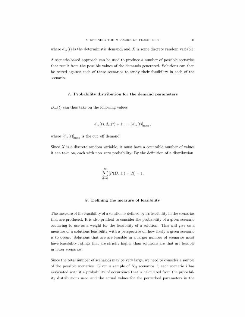
8. DEFINING THE MEASURE OF FEASIBILITY 41

where dm(t) is the deterministic demand, and X is some discrete random variable.

A scenario-based approach can be used to produce a number of possible scenarios

that result from the possible values of the demands generated. Solutions can then

be tested against each of these scenarios to study their feasibility in each of the

scenarios.

7. Probability distribution for the demand parameters

Dm(t) can thus take on the following values

dm(t), dm(t) + 1, . . . , [dm(t)]max ,

where [dm(t)]max is the cut–off demand.

Since X is a discrete random variable, it must have a countable number of values

it can take on, each with non–zero probability. By the definition of a distribution

∞∑d=0

[P (Dm(t) = d)] = 1.

8. Defining the measure of feasibility

The measure of the feasibility of a solution is defined by its feasibility in the scenarios

that are produced. It is also prudent to consider the probability of a given scenario

occurring to use as a weight for the feasibility of a solution. This will give us a

measure of a solutions feasibility with a perspective on how likely a given scenario

is to occur. Solutions that are are feasible in a larger number of scenarios must

have feasibility ratings that are strictly higher than solutions are that are feasible

in fewer scenarios.

Since the total number of scenarios may be very large, we need to consider a sample

of the possible scenarios. Given a sample of NQ scenarios I, each scenario i has

associated with it a probability of occurrence that is calculated from the probabil-

ity distributions used and the actual values for the perturbed parameters in the


scenario. For a scenario with a set of demand parameters δ, the probability of the

scenario is given by

P δi =

T∏t=0

P (D(t) = δ(t)).

Let φi be an indicator function for scenario i that acts on a candidate solution s,

and is defined as

φi(s) =

1 if s is feasible in scenario i

0 if s in not feasible in scenario i,

If we let Pi represent the probability of occurrence of scenario i, let F (s) represent

the feasibility of a solution s, and let Z be the maximum number of scenarios, then

we can then precisely define the measure of feasibility of a solution s in the following

way

F (s) =

Z∑i

Piφi(s).

This measure has some useful properties. The first is that there are lower and upper

bounds on the measure. If a solution is feasible in no scenarios, it takes the lowest

value of the measure, 0. If a solution satisfies all of the scenarios, it will take the

maximum value, 1.

The second useful property is that due to the behaviour of the indicator function

φi, the measure coincides with the probability of any of the scenarios occurring

for which s is feasible. Higher measures of feasibility are thus directly linked to

solutions that are more likely to satisfy a randomly generated scenario.

Typically, the number of scenarios is quite large, with many scenarios having a very

small probability of occurrence. It is thus more tractable to generate a sample of the

set of all possible scenarios (without replacement).We still retain all of the properties

described above if we normalise the measure with the total probability of occurrence

of all the scenarios in the sample. If we let Q be the set of sample scenarios, and

nQ be the cardinality of the set Q, then we can define the normalisation constant

8. DEFINING THE MEASURE OF FEASIBILITY 43

λ as

λ =

(nQ∑i=0

Pi

)−1.

The measure of feasibility is then generalised to

F (s) = λ

nQ∑i=0

Piφi(s).

This expression gives a normalised measure of feasibility in the sample space defined

by Q.

CHAPTER 6

Refining the model

This chapter covers refinements to the model to make it more tractable. These

include the relaxation of a particular class of constraints, the separability of the

model, and the effect of simulating multiple populations in the process of solving

the model.

1. Constraint relaxation

As noted in a previous chapter, a modified genetic algorithm performed poorly when

attempting to generate solutions in a uniformly random way. A co–evolutionary

algorithm will require at least some feasible solutions in its initial population in

order to generate fitter, feasible solutions.

The low number of feasible solutions indicate that the constraints place restrictions

on the system that limit the number of feasible solutions drastically. As a first step,

we can examine the model and check whether there are any classes of constraints

that can be relaxed in such a way that the optimal solution will remain the same.

For the optimal solution to remain the same, we must guarantee that all new solu-

tions have a greater objective function value than the original solutions. Consider

the objective function given by (1.1).

All costs in the problem are positive numbers, and all of the decision and state

variables that multiply these costs are restricted to take on non–negative values.

The size of the feasible set of solutions can be increased by relaxing any of the

bounds on hi(t), fi(t) and uij(t). This however, may reduce the value of the

optimal solution. One approach to deal with this is to set up and solve a sequence

of problems where the bounds on hi(t), fi(t) and uij(t) are decreased in increments,

finally reaching their original values.

45

46 6. REFINING THE MODEL

Consider the functions that define the dynamics of the state variables (2.1) and

(2.2).

The state equations show that only the hiring variables, hi(t), have a consistent

effect of increasing the state variables xi(t + 1). Since hi(t) and xi(t + 1) only

occur with positive costs in the objective function, increasing hi(t) will result in an

increase of the objective function.

In an analogous way, decreasing fi(t) will have a consistent effect of increasing

the state variables xi(t + 1). However, reducing the bounds on the variables fi(t)

introduces the possibility that the optimal solution to the original problem is not

feasible in the new problem.

Thus hi(t) is the only decision variable whose bounds we can increase while guar-

anteeing that the optimal solution to the original problem will remain feasible in

the new problem.

The only equation that directly controls the upper bounds on the variables hi(t)

are the hiring bound constraints,

hi(t) ≤ bhi (t), i = 1, . . . , N.

By increasing the value of each bhi (t) by some number, we can relax the hiring

bound constraints and allow for the generation of feasible solutions in the initial

population. The new bound constraints are then

hi(t) ≤ bhi (t) + βhi (t), i = 1, . . . , N.

The bound constant can be factored so that

hi(t) ≤ b′hi (t), i = 1, . . . , N,

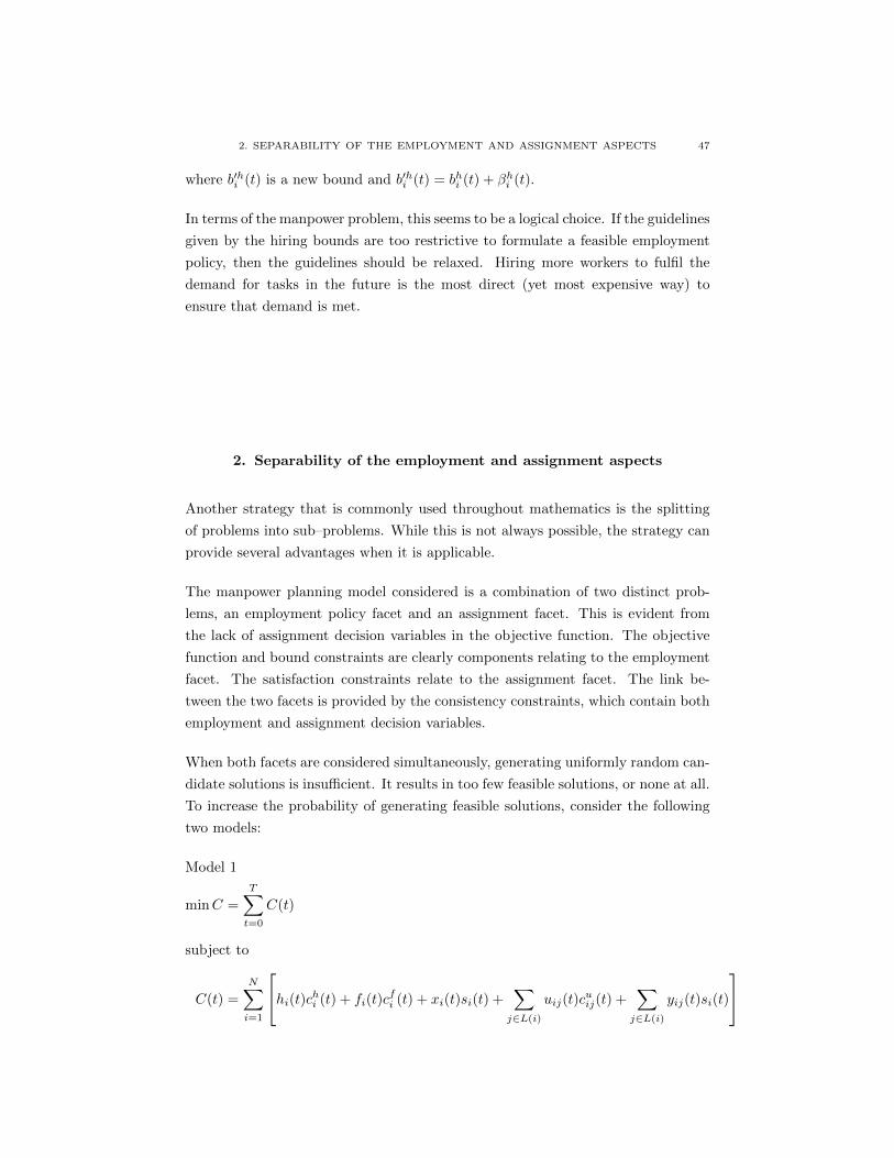
2. SEPARABILITY OF THE EMPLOYMENT AND ASSIGNMENT ASPECTS 47

where b′hi (t) is a new bound and b′hi (t) = bhi (t) + βhi (t).

In terms of the manpower problem, this seems to be a logical choice. If the guidelines

given by the hiring bounds are too restrictive to formulate a feasible employment

policy, then the guidelines should be relaxed. Hiring more workers to fulfil the

demand for tasks in the future is the most direct (yet most expensive way) to

ensure that demand is met.

2. Separability of the employment and assignment aspects

Another strategy that is commonly used throughout mathematics is the splitting

of problems into sub–problems. While this is not always possible, the strategy can

provide several advantages when it is applicable.

The manpower planning model considered is a combination of two distinct prob-

lems, an employment policy facet and an assignment facet. This is evident from

the lack of assignment decision variables in the objective function. The objective

function and bound constraints are clearly components relating to the employment

facet. The satisfaction constraints relate to the assignment facet. The link be-

tween the two facets is provided by the consistency constraints, which contain both

employment and assignment decision variables.

When both facets are considered simultaneously, generating uniformly random can-

didate solutions is insufficient. It results in too few feasible solutions, or none at all.

To increase the probability of generating feasible solutions, consider the following

two models:

Model 1

minC =

T∑t=0

C(t)

subject to

C(t) =

N∑i=1

hi(t)chi (t) + fi(t)cfi (t) + xi(t)si(t) +

∑j∈L(i)

uij(t)cuij(t) +

∑j∈L(i)

yij(t)si(t)


with the constraints

hi(t) ≤ b′hi (t), i = 1, . . . , N

fi(t) ≤ bfi (t), i = 1, . . . , N

uij(t) ≤ buij(t), i = 1, . . . , N, j ∈ L(i)

and

Model 2

min

N∑i=1

∑m∈M(i)

vim

with the constraints ∑i|m∈M(i)

vim(t) ≥ dm(t), m = 1, . . . ,M

∑m∈M(i)

vim(0) ≤ xi(0), i = 1, . . . , N

Model 1 is the employment aspect of the original model, and Model 2 is the assign-

ment aspect of the original model with an additional objective function specified.

The lack of assignment control variables in the original model’s objective function

forces us to specify an objective function if we wish to consider Model 2 as an

optimisation problem. The objective function is specified in such a way that it is

diametrically opposed to the demand constraints.

Model 1 has the trivial solution where all decision variables take on zero values, so

there is no need to solve the model. The initial population that is generated in a

uniformly random way should be passed directly to the original model.

Mathematically, the demand constraints only place a lower bound on combination

of assignment variables and do not specify the maximum values the variables can

take in this space. Without an objective function that is diametrically opposed

to the constraints, Model 2 becomes trivial to solve, with solutions taking on the

maximum values possible. The practical interpretation of the objective functions

is that assigning the minimum number of workers required would free up workers

so that they could be assigned to other tasks.

Most consistency constraints are conspicuously absent from either model for two

specific reasons. Firstly, the consistency constraints mix assignment and employ-

ment control variables (through the state variables xi(t) and decision variables

vim(t) ). In the context of these models, they cannot be specified as being a part of

3. THE POWER OF MULTIPLE POPULATIONS 49

either, since this mixes the solutions of both models. Secondly, the consistency con-

straints are the most restrictive constraints on the system. By solving these models

first, we are more likely to generate solutions that are feasible in the original model.

Solving both models would not necessarily give the optimal solution to the problem,

as they are only portions of the original problem. However, a solution in the

original model, when separated, is certainly a solution in both of these models. By

considering the two facets in isolation we decrease the complexity significantly and

allow for a greater possibility of generating feasible solutions.

By using a co–evolutionary algorithm to solve each model, we will be supplied

with candidate employment solutions and candidate assignment solutions. These

solutions can then be combined and used as members of an initial population in

the original model.

3. The power of multiple populations

Co–evolutionary algorithms differ from evolutionary algorithms in one major sense:

co–evolutionary algorithms simulate multiple interacting populations. As a result

of this, the interactions between the populations must be modelled. The overall

fitness of an individual is thus not only dependent on its usual fitness, but also on

how it interacts with other populations.

Co–operative co–evolutionary algorithms are a type of algorithm that use multiple

populations co–operating to reach solutions for a problem. An obvious application

of this is the separability of certain aspects of the problem. As an example, con-

sider two variables in an objective function that are not coupled. Adjusting one

variable while holding the other constant will give an indication of what effect the

variable has on the value of the objective function. Populations simulating each

of these variables independently would then allow an optimal solution to be found

by combining the results of both populations. So separately, the populations only

model some aspect of the original model, but when the populations cooperate they

form a complete solution to the model.

The co–operative approach can be used to model the employment and assignment

aspects of the manpower planning model. The solutions can then be combined and

used to provide candidate solutions for the complete model.


Figure 6.1. Overall solution space

Competitive co–evolutionary algorithms are a type of algorithm that simulate the

interactions of multiple populations that compete with one another. The overall

effect is still to improve the solutions to a problem, but the effect on individual

members of each population might be detrimental.

The competitive approach can be utilised by considering a predator–prey model.

The solutions are modelled as a prey population and the set of constraints are

modelled as a predator population. The predators and prey populations interact

in some way, with the predators eliminating some of the prey. Thus, solutions

that fulfil the constraints survive, while those that do not are eliminated from

the prey population. In this way, solutions that satisfy the constraints have a

greater probability of being chosen for breeding operations. When the algorithm

terminated, a larger set of solutions that satisfy the constraints are available.

Multiple populations can also be used when separating the employment and assign-

ment aspects of the manpower model. The original model has a large number of

rigorous constraints and variables. Consider the qualitative Figure 6.1 representing

the solution space of the original model.

The small pockets of feasible solutions are difficult to find using standard methods

for generating an initial population.

By splitting the original model into Model 1 and Model 2, we are left with two

solution spaces to consider, but each of which has less constraints and variables

3. THE POWER OF MULTIPLE POPULATIONS 51

Figure 6.2. Employment solution space

Figure 6.3. Assignment solution space

than the original problem. In addition to this, the effects of the constraints for

each of the models is less restrictive. This results in the qualitative representation

given by Figure 6.2 and Figure 6.3.

A method of generating uniformly random solutions is now much more likely to

result in feasible solutions.

The solutions from these two models can then be combined in such a way that

they produce solutions in the original model. Solutions in the original model are


produced by the product of the solution populations in Model 1 and Model 2. Thus,

1000 employment solutions combined with 1000 assignment solutions result in 1 000

000 solutions in the original problem. We can thus cover a far larger part of the

original solution space and focus on areas that are more likely to contain feasible

solutions.

4. Objective function minimisation versus feasibility, resource usage

Given the nature of the manpower planning model, it is necessary to investigate

what is expected of the outputs. Given that it has been cast as an optimisation

problem, minimisation of the objective function appears to be the overriding con-

cern. Yet the previous sections have highlighted the need for solutions that are

feasible and insensitive to small changes in certain constraint parameters. Solu-

tions of this nature should also be produced in a reasonable amount of time, with

a realistic amount of resources.

The discussion of the manpower planning problem given in [22] considers the man-

power planning requirements of the US armed forces. The need for this entity to

meet its obligations while minimising costs is paramount. It is expected to be able

to successfully carry out missions relating to several large scale conflicts simultane-

ously. This is no simple problem, as the complex organisation structure (including

ranks, experience, age, and specialisation) lead to a large number of worker types

and complex training programs. The demands to be met for engaging in conflicts

is inherently uncertain, and the planning horizon can extend to the order of several

years. Stochastic attrition must also be taken into account to realistically model

the system.

Solutions to this kind of problem cannot be sensitive to slight changes in the values

of uncertain parameters in the constraints. Even if the cost of such solutions is

considerably lower than others, they lose their usefulness as soon as they become

infeasible. When combat readiness of a unit depends on such solutions, they must

be feasible for a range of changes to the uncertain parameters.

These arguments clearly show that the minimisation of the objective function is

not the primary goal. The overriding goal is to provide feasible solutions that are

insensitive to changes in uncertain parameters. The solutions with the minimum

cost from this result set can then be chosen and implemented. The trade off between

higher costs for increased insensitivity to uncertain parameters is one that should

be made by the organisation. The manpower planning model should provide the

4. OBJECTIVE FUNCTION MINIMISATION VERSUS FEASIBILITY, RESOURCE USAGE 53

organisation with the relevant information to decide on the degree of trade–off they

desire.

CHAPTER 7

The algorithm

1. Overview of the algorithm

To solve the manpower planning model, a mixed cooperative and competitive co–

evolutionary algorithm is used.

The first step is a to consider the co–evolutionary algorithms associated with Model

1 and Model 2. Each of these are run to produce employment and assignment solu-

tions. These are then combined to produce initial populations for a co–evolutionary

algorithm associated with the original model. This allows the majority of the con-

straints to be checked before the original model is even considered. This mechanism

to generate an initial population for the original model is thus more effective that

a method of generating uniformly random solutions.

Each of the two initial co–evolutionary algorithms solve a model that is less restric-

tive than the original model. The key idea is that a feasible solution of the original

model, when separated, must be a feasible solution in Model 1 and Model 2. Let

m1 and m2 be maps from a feasible solution s0 in the original model to solutions

s1 and s2 in each of the other models respectively. Then

s1 = m1(s0)

s2 = m2(s0).

are both feasible solutions in the spaces of the respective model by virtue of the

fact that they only contain a subset of the constraints from the original model.

Each of the co–evolutionary algorithms consists of one prey and one predator pop-

ulation. The predators perform predation operations on the prey, affecting their

chances of passing into the next generation. The remaining prey then breed, produc-

ing new solutions, and the process continues until some stop condition is reached.

55

56 7. THE ALGORITHM

Prey represent solutions of the control variables, thus representing a complete so-

lution. The state variables can be computed from the values of the decision vari-

ables, and the objective function can then be evaluated. Predators represent the

constraints for a particular model, with a measure of their effectiveness against

solutions.

In this implementation of the algorithm, we allow the prey populations to evolve so

that fitter solutions can be generated. The predator populations, by contrast, are

kept static and do not evolve. The reason for this is straightforward: we want our

solutions to satisfy the constraints we specify initially, not some other constraints

that are the result of genetic operations.

When an interaction takes place between a solution and a constraint, there are

two possibilities. If the solution satisfies the constraint, it survives and continues

breeding. If it does not satisfy the constraint, it is eliminated and the constraint’s

fitness is increased. After several generations, this gives us an excellent measure of

which constraints in the problem are trivially satisfied and which constraints are

extremely difficult to satisfy.

2. IMPLEMENTATION 57

Formally, the steps for the algorithm are as follows:

Input : Problem dataOutput: List of fittest, feasible solutionsInitialise initial prey population, predator population;

while Stop conditions not reached dofor offspring ← numberOfOffspring do

breeders = SelectBreeders(preyPopulation, numberOfOffspring);

foreach breedingPair in breeders dooffspringPair = Breed(breedingPair)offspringPair = Mutate(offspringPair)preyPopulation = preyPopulation

⋃offspringPair

end

end

for attacks = 1 to maximumAttacks dopredator = SelectPredator(predatorPopulation);

prey = SelectRandomPrey(preyPopulation);

if predator Kills Prey thenpreyPopulation = preyPopulation \{prey};predator.fitness = predator.fitness + 1;

end

end

endAlgorithm 2: Co–evolutionary algorithm

2. Implementation

The algorithm is implemented in C#, a strongly typed, object–oriented language

based on Microsoft’s .NET platform. The language provides a structured environ-

ment to model the manpower planning model and the co–evolutionary algorithm

on an appropriate level of abstraction. The object-oriented nature of the language

allows concepts such as inheritance and polymorphism to assist in the abstraction

process.

The various test cases and the main problem were run on an AMD Athlon(tm)

64 X2 dual core processor 5400+, with 3.25 GB of RAM, running Windows XP

Professional and the required .NET 3.5 Framework.

A code profiling tool, NProf, was used to profile the code and target specific pieces

of the code that required optimisation to improve performance. FXCop, a tool that

checks conformance with Microsoft’s .NET Framework Design Guidelines was used

58 7. THE ALGORITHM

to ensure the guidelines were reasonably followed. Inheritance diagrams and code

documentation were generated using Graphviz and Doxygen.

3. Programming concepts

The principles underlying object oriented programming are expressed in a way that

allows one to model complex systems in a manner that is natural to the problem.

The ability to create user defined types (classes) allows one to capture the essential

aspects of the system that must be modelled, while maintaining a level of complexity

that is manageable.

In the case of the manpower planning problem, there are several different layers

that are modelled. The first is the actual manpower model, expressed in terms of

workers, tasks, costs, and so forth. Another level is the modelling of the algorithm,

its operations (such as mutation and breeding), and the members of the populations

(predators and prey). Finally, there is a mathematical layer that represents the

objective function, the balance equations and so on.

Object oriented programming revolves around three central principles: Encapsula-

tion, inheritance and polymorphism.

Encapsulation is the principle that is concerned with separating objects and hiding

the implementation of an objects behaviour from other objects. The objects should

clearly specify what operations are allowed to be performed on them by other ob-

jects, and which operations they are allowed to perform by themselves. The actual

implementation of methods in objects is hidden so that other objects behaviour is

not dependent on changes to these. This creates a distinct zone of demarcation for

objects (the clients) that access the methods of another object (the server). The

server exposes a set of interfaces, while hiding the implementation of these inter-

faces. This eliminates the dependency of the clients on the server’s implementation,

and they are only dependant on the interfaces. As an example, consider the task

information class. This class exposes certain information on which workers can per-

form a particular task. The public interface defined by this class is one that allows

a client to call the CanBePerformedBy method, passing in a task. The client can

then expect a list of workers that can perform the task to be returned. The internal

implementation is done via a lookup in a dictionary, but this is hidden from the

client.

public class TaskInfo

3. PROGRAMMING CONCEPTS 59

{

private Dictionary<Task, List<WorkerType>> _canBePerformedBy;

public List<WorkerType> CanBePerformedBy(Task task)

{

...

}

}

Inheritance allows for levels of abstraction by defining the shared properties of

groups of objects. The class defining the common behaviour of the other classes

is referred to as the base class, and classes inheriting from this are termed derived

classes. All classes that inherit from this class are guaranteed to satisfy the be-

haviour set out by the base class. This reduces the amount of code that would

otherwise be needed to model a problem. Inheritance also results in generalisations

of types, as the base class represents a generalisation of the derived classes. As

an example, a simple genetic algorithm manager type is defined to inherit from a

co–evolutionary algorithm type, and the base classes Run method is overridden.

public class SimpleGAManager : CoevolutionaryAlgorithm

{

...

}

public override void Run()

{

...

}

Figure 7.1 shows the detailed inheritance diagram for the Chromosome class. This

shows the classes that inherit from the chromosome class, as well as the various

member methods and variables applicable to each class. Figure 7.3 shows the

simplified inheritance diagram for the same class.

Figure 7.2 shows the collaboration diagram for the co–evolutionary algorithm class.

This shows the member variables of the co–evolutionary algorithm class, as well as

the various member methods and variables applicable to each object.

60 7. THE ALGORITHM

Figure 7.1. Detailed chromosome inheritance

Figure 7.4 shows the inheritance diagram for the Constraint class. This shows the

various classes that inherit from the Constraint class.

Polymorphism allows a disparate collection of objects that share the same base class

to be treated as a collection of the same objects. In this way, operations may be

performed on a collection of these objects without actually knowing the underlying

types of the objects. As an example, consider the abstract class Chromosome

abstract public class Chromosome : IComparable<Chromosome>

{

...

}


Figure 7.2. Co–evolutionary algorithm collaboration graph

Figure 7.3. Chromosome inheritance

62 7. THE ALGORITHM

Figure 7.4. Constraint inheritance

By definition, an abstract class cannot be instantiated. Even so, polymorphism can

be used to loop over a list of items that all inherit from the Chromosome class

foreach (Chromosome chromosome in preyPopulation.Item)

{

...

}

Another powerful concept is that of reflection. This allows a class to inspect its

own properties and possibly modify its behaviour. As an example, consider the

abstract Chromosome class. Since it is abstract, we cannot construct an instance

of it. At a point in the code where polymorphism is used to loop over a collection of

Chromosomes, information about the underlying class is needed. In the code below,

reflection is used to query the constructor information for the class underlying the

Chromosome object. This is then used to instantiate another instance of the type.

ConstructorInfo constructorInfo =


preyPopulation.Item[preyIndex].GetType().GetConstructor(

new Type[] { preyPopulation.Item[preyIndex].GetType() });

tempObject = constructorInfo.Invoke(

new object[] { preyPopulation.Item[preyIndex] });

CHAPTER 8

Test cases

This chapter considers three test cases, each of which considers a case of the man-

power planning model with certain characteristics. Each of the cases is small enough

to be checked using a brute force algorithm, allowing comparison of the optimal

solution with the solutions generated by the co–evolutionary algorithm.

1. Test case 1

Test case 1 considers a manpower planning model in which there is only a sin-

gle worker type, a single task, and no training. This is the most straightforward

scenario, where a single worker is only responsible for performing a single task.

The following information defines the test case

Table 8.1. Test case 1 - General information

General parametersNumber of constraints 14Number of decision variables 10Number of state variables 3

Table 8.2. Test case 1 - General parameters

General parametersT 3N 1m 1

Table 8.3. Test case 1 - Task information

TasksM(1) {1}

65

66 8. TEST CASES

Table 8.4. Test case 1 - Hiring bounds

Hiring boundsbh1 (t) ∀ t 2

Table 8.5. Test case 1 - Dismissal bounds

Dismissal bounds

bf1 (t) ∀ t 1

Table 8.6. Test case 1 - Demand

dm(t)t = 0 t = 1 t = 2 t = 3

m = 1 1 3 2 2

Table 8.7. Test case 1 - Hiring costs

Hiring costsch1 (t) ∀ t 1

Table 8.8. Test case 1 - Dismissal costs

Dismissal costs

cf1 (t) ∀ t 1.5

Table 8.9. Test case 1 - Salaries

Salariess1(t) ∀ t 0.7

Table 8.10. Test case 1 - Initial workers

Initial workersx1(0) 2

2. TEST CASE 1 - BRUTE FORCE ALGORITHM RESULTS 67

2. Test case 1 - Brute force algorithm results

The optimal solution given by the brute force algorithm returned a feasible solution

with an objective function value of 6.6. The values of the decision and state variables

are given in Table 8.11.

Table 8.11. Test case 1 - Optimal solution

Optimal solutionh1(0) 1h1(1) 0h1(2) 0f1(0) 0f1(1) 0f1(2) 0v1,1(0) 2v1,1(1) 3v1,1(2) 2v1,1(3) 3x1(0) 2x1(1) 3x1(2) 3x1(3) 3

68 8. TEST CASES

3. Test case 1 - Co–evolutionary algorithm results

The optimal solution given by the co–evolutionary algorithm returned a feasible

solution with an objective function value of 6.6. The values of the decision and

state variables are given in Table 8.12.

Table 8.12. Test case 1 - Co–evolutionary Optimal solution

Optimal solutionh1(0) 1h1(1) 0h1(2) 0f1(0) 0f1(1) 0f1(2) 0v1,1(0) 1v1,1(1) 3v1,1(2) 2v1,1(3) 3x1(0) 2x1(1) 3x1(2) 3x1(3) 3

The objective function value is the same as the value of the optimal solution

found by the brute force algorithm. Only assignment decision variable values differ

slightly. This is expected as the assignment decision variables do not affect values

of the objective function.

The sensitivity analysis sample was almost complete, with a coverage of 0.999. This

revealed that the optimal solution found had a feasibility measure of 0.594, and the

solution found by the co–evolutionary algorithm had a feasibility measure of 0.495.

The co–evolutionary algorithm found solutions with higher feasibility at a higher

cost. This is expected, as higher costs often involve hiring more workers, making

them available for increases in demand in the future.

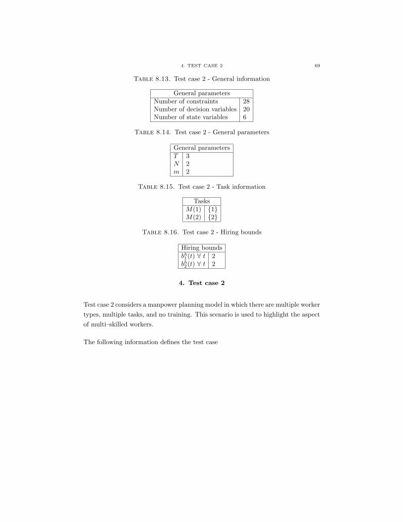
4. TEST CASE 2 69





Table 8.15. Test case 2 - Task information

TasksM(1) {1}M(2) {2}


Hiring boundsbh1 (t) ∀ t 2bh2 (t) ∀ t 2

4. Test case 2

Test case 2 considers a manpower planning model in which there are multiple worker

types, multiple tasks, and no training. This scenario is used to highlight the aspect

of multi–skilled workers.


70 8. TEST CASES


Dismissal bounds

bf1 (t) ∀ t 1

bf2 (t) ∀ t 1


dm(t)t = 0 t = 1 t = 2 t = 3

m = 1 1 2 1 1m = 2 0 1 2 2


Hiring costsch1 (t) ∀ t 1.2ch2 (t) ∀ t 1.5


Dismissal costs

cf1 (t) ∀ t 2

cf2 (t) ∀ t 2.4


Salariess1(t) ∀ t 1s2(t) ∀ t 1.2


Initial workersx1(0) 2x2(0) 1




with an objective function value of 12.3. The values of the decision and state

variables are given in Table 8.23.


Optimal solutionh1(0) 0h2(0) 0h1(1) 0h2(1) 1h1(2) 0h2(2) 0f1(0) 0f2(0) 0f1(1) 0f2(1) 0f1(2) 0f2(2) 0v1,2(0) 2v2,1(0) 0v1,2(1) 2v2,1(1) 1v1,2(2) 2v2,1(2) 2v1,2(3) 2v2,1(3) 2x1(0) 2x2(0) 1x1(1) 2x2(1) 1x1(2) 2x2(2) 2x1(3) 2x2(3) 2

72 8. TEST CASES


The solution given by the co–evolutionary algorithm returned a feasible solution

with an objective function value of 13.5. The values of the decision and state

variables are given in Table 8.24.


Optimal solutionh1(0) 0h2(0) 1h1(1) 0h2(1) 0h1(2) 0h2(2) 0f1(0) 0f2(0) 0f1(1) 0f2(1) 0f1(2) 0f2(2) 0v1,2(0) 2v2,1(0) 1v1,2(1) 2v2,1(1) 2v1,2(2) 1v2,1(2) 2v1,2(3) 2v2,1(3) 2x1(0) 2x2(0) 1x1(1) 2x2(1) 2x1(2) 2x2(2) 2x1(3) 2x2(3) 2

The objective function value of the solution found by the co–evolutionary algorithm

is only slightly higher than the value of optimal solution found by the brute force

algorithm.

6. TEST CASE 2 - CO–EVOLUTIONARY ALGORITHM RESULTS 73

The sensitivity analysis sample was almost complete (a coverage of 0.969). This

revealed that the optimal solution found by the brute force algorithm had a nor-

malised feasibility measure of 0.303, while the solution found by the co–evolutionary

algorithm had a normalised feasibility measure of 0.253.

The co–evolutionary algorithm found solutions with higher feasibility at a higher



74 8. TEST CASES





Table 8.27. Test case 3 - Tasks

Task informationM(1) {1}M(2) {1, 2}

Table 8.28. Test case 3 - Training information

TrainingL(1) {2}

7. Test case 3

Test case 3 considers a manpower planning model in which there are multiple worker

types, multiple tasks, and training programs for a subset of the worker types. This

is the most general scenario, where workers are responsible for various tasks and

are able to be trained to other worker types.


7. TEST CASE 3 75


Hiring boundsbh1 (t) ∀ t 2bh2 (t) ∀ t 2


Dismissal bounds

bf1 (t) ∀ t 1

bf2 (t) ∀ t 1

Table 8.31. Test case 3 - Training bounds

Training boundsbu12(t) ∀ t 1

Table 8.32. Test case 3 - Training times

Training timesτ12 1


dm(t)t = 0 t = 1 t = 2

m = 1 1 2 1m = 2 0 1 2


Hiring costsch1 (t) ∀ t 1.2ch2 (t) ∀ t 1.5


Dismissal costs

cf1 (t) ∀ t 2

cf2 (t) ∀ t 2.4

Table 8.36. Test case 3 - Training costs

Training costscu12(t) ∀ t 0.5


Salariess1(t) ∀ t 1s2(t) ∀ t 1.2

76 8. TEST CASES


Initial workersx1(0) 2x2(0) 1

Table 8.39. Test case 3 - Initial workers in training

Initial workers in trainingy12(0) 0




with an objective function value of 7.9. The values of the decision and state variables

are given in Table 8.40.


Optimal solutionh1(0) 0h2(0) 0h1(1) 0h2(1) 1f1(0) 0f2(0) 0f1(1) 0f2(1) 0u1,2(0) 0u1,2(1) 0v1,2(0) 2v2,2(0) 0v2,1(0) 0v1,2(1) 2v2,2(1) 0v2,1(1) 1v1,2(2) 2v2,2(2) 0v2,1(2) 2x1(0) 2x2(0) 1x1(1) 2x2(1) 1x1(2) 2x2(2) 2y1,2(0) 0y1,2(1) 0y1,2(2) 0

78 8. TEST CASES


The optimal solution given by the co–evolutionary algorithm returned a feasible

solution with an objective function value of 9.4. The values of the decision and

state variables are given in Table 8.41.


Optimal solutionh1(0) 0h2(0) 0h1(1) 0h2(1) 2f1(0) 0f2(0) 0f1(1) 0f2(1) 0u1,2(0) 0u1,2(1) 0v1,2(0) 2v2,2(0) 0v2,1(0) 1v1,2(1) 2v2,2(1) 0v2,1(1) 1v1,2(2) 1v2,2(2) 1v2,1(2) 2x1(0) 2x2(0) 1x1(1) 2x2(1) 1x1(2) 2x2(2) 3y1,2(0) 0y1,2(1) 0y1,2(2) 0


is only slightly higher than the value of optimal solution found by the brute force

algorithm.

The sensitivity analysis sample was almost complete (a coverage of 0.999). This re-

vealed that the optimal solution found by the brute force algorithm has a normalised

9. TEST CASE 3 - CO–EVOLUTIONARY ALGORITHM RESULTS 79

feasibility measure of 0.457, while the best solution found by the co–evolutionary

algorithm had a normalised feasibility measure of 0.381.

The co–evoltionary algorithm found solutions with higher feasibility at a higher



CHAPTER 9

Main problem

The following chapter considers the main problem. This problem is adapted from

the sample problem in [3], but the problems share the same optimal solution.

1. Main problem

The following information defines the main problem, which is adapted from [3],

where an optimal solution was found. It is a realistically sized manpower plan-

ning problem, with multi–skilled workers, training programs, and a restrictive set

of demand parameters. The co–evolutionary algorithm will be used to solve the

problem, and its solutions compared with the solution found in [3]. A feasibility

analysis will then be done on the solutions.

Table 9.1. Main problem - General information


Table 9.2. Main problem - General parameters


Table 9.3. Main problem - Task information

TasksM(1) {1}M(2) {2}M(3) {1, 2}

81

82 9. MAIN PROBLEM

Table 9.4. Main problem - Training information

TrainingL(1) {3}L(2) {3}L(3) {}

Table 9.5. Main problem - Hiring bounds

Hiring boundsbh1 (t) ∀ t 4bh2 (t) ∀ t 3bh3 (t) ∀ t 2

Table 9.6. Main problem - Dismissal bounds

Dismissal bounds

bf1 (t) ∀ t 2

bf2 (t) ∀ t 2

bf3 (t) ∀ t 2

Table 9.7. Main problem - Training bounds

Training boundsbu13(t) ∀ t 2bu23(t) ∀ t 2

Table 9.8. Main problem - Demand

dm(t)t = 0 t = 1 t = 2 t = 3 t = 4 t = 5 t = 6 t = 7 t = 8 t = 9

m = 1 2 2 3 2 1 2 6 2 2 6m = 2 2 3 1 2 7 2 2 8 5 1

Table 9.9. Main problem - Hiring costs

Hiring costsch1 (t) ∀ t 1.2ch2 (t) ∀ t 1.5ch3 (t) ∀ t 3.0

Table 9.10. Main problem - Dismissal costs

Dismissal costs

cf1 (t) ∀ t 2.0

cf2 (t) ∀ t 2.4

cf3 (t) ∀ t 4.0

1. MAIN PROBLEM 83

Table 9.11. Main problem - Salaries

Salariess1(t) ∀ t 1.0s2(t) ∀ t 1.2s3(t) ∀ t 2.0

Table 9.12. Main problem - Training costs

Training costscu23(t) ∀ t 0.3cu13(t) ∀ t 0.5

Table 9.13. Main problem - Training times

Training timesτ13 2τ23 1

Table 9.14. Main problem - Initial workers

Initial workersx1(0) 2x2(0) 2x3(0) 0

Table 9.15. Main problem - Initial workers in training

Initial workers in trainingy13 0y23 0

84 9. MAIN PROBLEM

Table 9.16. Main problem optimal solution - hiring variables

Optimal solution - hiring variablesh1(0) 0h2(0) 0h3(0) 1h1(1) 0h2(1) 0h3(1) 0h1(2) 0h2(2) 2h3(2) 0h1(3) 0h2(3) 2h3(3) 0h1(4) 0h2(4) 0h3(4) 0h1(5) 1h2(5) 0h3(5) 0h1(6) 0h2(6) 0h3(6) 0h1(7) 0h2(7) 0h3(7) 0h1(8) 0h2(8) 0h3(8) 0

2. Optimal solution results

2. OPTIMAL SOLUTION RESULTS 85

Table 9.17. Optimal solution - dismissal variables

Optimal solution - dismissal variablesf1(0) 0f2(0) 0f3(0) 0f1(1) 0f2(1) 0f3(1) 0f1(2) 0f2(2) 0f3(2) 0f1(3) 0f2(3) 0f3(3) 0f1(4) 0f2(4) 0f3(4) 0f1(5) 0f2(5) 0f3(5) 0f1(6) 0f2(6) 0f3(6) 0f1(7) 0f2(7) 2f3(7) 0f1(8) 0f2(8) 0f3(8) 0

86 9. MAIN PROBLEM

Table 9.18. Optimal solution - training variables

Optimal solution - training variablesu1,3(0) 0u2,3(0) 0u1,3(1) 0u2,3(1) 0u1,3(2) 0u2,3(2) 0u1,3(3) 1u2,3(3) 0u1,3(4) 0u2,3(4) 2u1,3(5) 0u2,3(5) 0u1,3(6) 0u2,3(6) 0u1,3(7) 0u2,3(7) 0u1,3(8) 0u2,3(8) 0

2. OPTIMAL SOLUTION RESULTS 87

Table 9.19. Optimal solution - assignment variables

Optimal solution - assignment variablesv1,1(0) 2v2,2(0) 2v3,1(0) 0v3,2(0) 0v1,1(1) 2v2,2(1) 2v3,1(1) 0v3,2(1) 1v1,1(2) 2v2,2(2) 2v3,1(2) 1v3,2(2) 0v1,1(3) 2v2,2(3) 4v3,1(3) 1v3,2(3) 0v1,1(4) 1v2,2(4) 6v3,1(4) 0v3,2(4) 1v1,1(5) 1v2,2(5) 4v3,1(5) 1v3,2(5) 0v1,1(6) 2v2,2(6) 4v3,1(6) 4v3,2(6) 0v1,1(7) 2v2,2(7) 4v3,1(7) 0v3,2(7) 4v1,1(8) 2v2,2(8) 2v3,1(8) 1v3,2(8) 3v1,1(9) 2v2,2(9) 2v3,1(9) 4v3,2(9) 0

88 9. MAIN PROBLEM

Table 9.20. Main problem co–evolutionary solution - hiring variables

Co–evolutionary solution - hiring variablesh1(0) 1h2(0) 2h3(0) 2h1(1) 1h2(1) 0h3(1) 3h1(2) 3h2(2) 1h3(2) 3h1(3) 0h2(3) 0h3(3) 1h1(4) 0h2(4) 0h3(4) 0h1(5) 0h2(5) 0h3(5) 0h1(6) 0h2(6) 0h3(6) 0h1(7) 1h2(7) 1h3(7) 0h1(8) 1h2(8) 3h3(8) 0

3. Co–evolutionary algorithm results


is 283.8, compared to the optimal solution which has an objective function value of

119.1.

The sensitivity analysis sample had a coverage of 0.277. The actual optimal value

was found to have a normalised feasibility measure of 0.152, while the best solution

found by the co–evolutionary algorithm had a normalised feasibility measure of

0.524. This shows that while the cost of the solution found by the co–evolutionary

algorithm is higher, it is far less sensitive to changes in the demand parameters.

3. CO–EVOLUTIONARY ALGORITHM RESULTS 89

Table 9.21. Main problem co–evolutionary solution - dismissal variables

Co–evolutionary solution - dismissal variablesf1(0) 0f2(0) 0f3(0) 0f1(1) 0f2(1) 0f3(1) 0f1(2) 0f2(2) 0f3(2) 0f1(3) 0f2(3) 0f3(3) 0f1(4) 0f2(4) 0f3(4) 0f1(5) 0f2(5) 0f3(5) 0f1(6) 0f2(6) 0f3(6) 0f1(7) 0f2(7) 0f3(7) 0f1(8) 0f2(8) 0f3(8) 0

90 9. MAIN PROBLEM

Table 9.22. Main problem co–evolutionary solution - training variables

Co–evolutionary solution - training variablesu1,3(0) 2u2,3(0) 0u1,3(1) 0u2,3(1) 1u1,3(2) 0u2,3(2) 0u1,3(3) 2u2,3(3) 2u1,3(4) 0u2,3(4) 0u1,3(5) 0u2,3(5) 0u1,3(6) 0u2,3(6) 0u1,3(7) 1u2,3(7) 0u1,3(8) 2u2,3(8) 1


Table 9.23. Main problem co–evolutionary solution - assignment variables

Co–evolutionary solution - assignment variablesv1,1(0) 2v2,2(0) 2v3,1(0) 0v3,2(0) 0v1,1(1) 2v2,2(1) 4v3,1(1) 0v3,2(1) 2v1,1(2) 3v2,2(2) 0v3,1(2) 4v3,2(2) 1v1,1(3) 2v2,2(3) 3v3,1(3) 0v3,2(3) 0v1,1(4) 2v2,2(4) 3v3,1(4) 1v3,2(4) 6v1,1(5) 3v2,2(5) 3v3,1(5) 1v3,2(5) 2v1,1(6) 3v2,2(6) 3v3,1(6) 8v3,2(6) 1v1,1(7) 3v2,2(7) 4v3,1(7) 0v3,2(7) 8v1,1(8) 3v2,2(8) 6v3,1(8) 3v3,2(8) 2v1,1(9) 5v2,2(9) 2v3,1(9) 2v3,2(9) 0

92 9. MAIN PROBLEM

Table 9.24. Main problem co–evolutionary solution - available workers

Co–evolutionary solution - available workersx1(0) 2x2(0) 2x3(0) 0x1(1) 3x2(1) 4x3(1) 2x1(2) 4x2(2) 4x3(2) 5x1(3) 7x2(3) 5x3(3) 8x1(4) 7x2(4) 5x3(4) 9x1(5) 7x2(5) 5x3(5) 9x1(6) 7x2(6) 5x3(6) 9x1(7) 7x2(7) 5x3(7) 9x1(8) 8x2(8) 6x3(8) 9x1(9) 9x2(9) 9x3(9) 9


Table 9.25. Main problem co–evolutionary solution - available workers

Co–evolutionary solution - workers in trainingy1,3(0) 0y2,3(0) 0y1,3(1) 2y2,3(1) 0y1,3(2) 2y2,3(2) 1y1,3(3) 0y2,3(3) 0y1,3(4) 2y2,3(4) 2y1,3(5) 2y2,3(5) 0y1,3(6) 0y2,3(6) 0y1,3(7) 0y2,3(7) 0y1,3(8) 1y2,3(8) 0y1,3(9) 3y2,3(9) 1

CHAPTER 10

Conclusion

In this dissertation we reviewed the manpower planning problem and its role in

managing the resources of an organisation to meet its demands for the future.

The manpower planning problem was cast as a mathematical model. The model

allows for various classes of constraints to model the restrictions on the system,

mechanisms for hiring, dismissing, training and assigning workers to tasks. Balance

equations were introduced to track the number of workers, as well as the number of

workers in training. The balance equations, objective function and constraints were

analysed. It was noted that while the objective function is linear in the decision and

state variables, the state variables are non–linear. The non–linearity is a result of

the time delay terms in the state equations. The overall effect is that the objective

function and several classes of constraints are non–linear.

Various alternatives for modelling the problem were highlighted, and their strengths

and weaknesses discussed. The exponential problem faced when solving problems

with gradually larger numbers of variables was discussed, and the effect on the man-

power planning model was considered. It was found that the restrictive constraints

in the manpower planning model, along with the exponential problem, result in a

rapidly decreasing ratio of feasible solutions to candidate solutions as the size of

the problem increases.

The discrete nature of the problem was analysed and compared to methods used to

solve continuous problems. A modified genetic algorithm was used to attempt to

solve a medium sized manpower planning problem, and it was found that the algo-

rithm could not progress due to a lack of feasible solutions in the initial generation

of candidate solutions.

The sensitivity analysis of solutions was then considered as integral to analysing

solutions to the manpower planning model. While optimisation problems focus

primarily on optimising solutions with respect to the objective function, it may

95

96 10. CONCLUSION

be more important to also minimise the sensitivity of solutions to changes in pa-

rameters within constraints. In the case of the manpower planning model, these

parameters are the demands for tasks in the future. Given the inherent uncertainty

of the demand parameters, it is prudent to consider the feasibility of the solutions

when the parameters are altered. A measure of feasibility was defined that coin-

cided with the probability of a solution being feasible across a range of scenarios.

This definition was extended to allow for a only a sample of the total number of

the scenarios to be considered.

Methods for refining the model and making the model more tractable to solve

were then introduced. The hiring bound constraints were highlighted as a class of

constraints that could be relaxed to introduce a larger number of initial, feasible

solutions. The employment and assignment aspects were then separated from the

original model into two separate models. These new models were then shown to

encapsulate some aspects of the original model, and methods for utilising these

models to solve the original problem were discussed. The use of multiple populations

was discussed and it was found that these could be applied to the two separated

models to produce a higher number of initial, feasible solutions in the manpower

planning model.

The co–evolutionary algorithm was then introduced and its method of operation

defined. The algorithm uses a predator–prey model to simulate an optimisation

problem with candidate solutions and constraints. The solutions are modelled as a

prey population that breed new solutions to the problem, and a predator population

was used to model the constraints in the system. Interactions between the predators

and prey result in solutions that do not satisfy the constraints being eliminated

gradually.

Three small test cases that could be checked with a brute force algorithm were then

considered. It was shown that in some cases the co–evolutionary algorithm found

the optimal solutions. In cases where it did not, the solutions objective function

values differed only slightly. The feasibility of the solutions was also analysed.

A realistically sized manpower problem was then considered. The optimal solution

found in [3] was compared to the best solution found by the co–evolutionary al-

gorithm. The co–evolutionary algorithm produced a result with a higher objective

function value, but had a much higher feasibility rating than the optimal solution.

This is preferable as the uncertainty in the demand constraints’ parameters require

a set of decisions that are reasonably insensitive to changes in these parameters.

APPENDIX A

Calculations

1. Initial conditions for training

This section considers the special case where χij 6= 0.

A set of initial conditions yij(0) = χij is not sufficient to determine a unique past

for the problem. There are many states of the problem for times t < 0 that will lead

to the initial conditions being satisfied, with differing effects on the state variables

for t > 0. Thus, while we know how many workers are in training from one type

to another at time t = 0, it is unknown how long each of the workers has been in

training. This prevents us from knowing when workers should re–enter the pool of

assignable workers. A unique past is guaranteed in the special case where χij = 0

∀ χij .

This can be illustrated by considering the balance equations which govern the dy-

namics of the system,


uij(t) +∑

j|i∈L(j)

uji(t− τji)

yij(t+ 1) = yij(t) + uij(t)− uij(t− τij).

Setting t = 0 gives

xi(1) = xi(0) + hi(0)− fi(0)−∑j∈L(i)

uij(0) +∑

j|i∈L(j)

uji(−τji)

yij(1) = yij(0) + uij(0)− uij(−τij).

All variables are determined for the problems with the exception of the terms

uij(−τij). These terms represent the control variables for training decisions that

were made in the past (t < 0). By setting t = 1, . . . , T , we note that we require the

97

98 A. CALCULATIONS

information for some uij(t) where t < 0. Specifically, we require information for all

uij(t), t = −1, . . . ,−τij , i = 1, . . . , N, j ∈ L(i).

To generalise the initial conditions, this information needs to be added to the model.

Thus, the knowledge of control variables in the previous time steps

uij(t), i = 1, . . . , N, j ∈ L(i), t = −1, . . . ,−τij ,

and the initial conditions

yij = χij

specify the problem uniquely when there are workers in training at t = 0.

2. Maximum cardinality of the sets L(i) and M(i)

Given a problem with N worker types and r tasks, it is useful to have an upper

bound on the number of training variables (uij) and task variables (vim) as simple

functions of N and r. This can be done by making some assumptions about the

structure of the problem.

To establish an upper bound, some basic assumptions must be made. Let the

workforce exhibit a hierarchical structure, where workers who are higher in the

hierarchy are capable of performing more tasks than workers lower in the hierarchy.

We assume the tasks exhibit the same structure. A worker lower down in the

hierarchy can be trained to any higher level in the hierarchy. Training is not circular,

so for a given worker type i, there exists no sequence of training programs that will

result in the worker being trained back to type i. The worker type at the top of the

hierarchy is capable of performing all tasks. If worker type i can perform n number

of tasks, worker type i− 1 can perform n− 1 number of tasks. This results in each

a worker type at each lower level in the hierarchy being able to perform one less

task than a worker at the higher level. We further assume that the number of tasks

is equal to, or exceeds the number of worker types.

The above assumptions result in worker type 1 having training programs to all

worker types, and worker type N having no training programs. In general

cardL(i) = N − i

2. MAXIMUM CARDINALITY OF THE SETS L(I) AND M(I) 99

and

N∑i=1

cardL(i)

=

N∑i=1

(N − i)

=

N∑i=1

N −N∑i=1

i

= N(N)− N(N + 1)

2

=N

2(N − 1).

The above assumptions also give the following expression for the cardinality of M(i)

cardM(i) = r − (N − i)

and

N∑i=1

cardM(i)

=

N∑i=1

(r − (N − i))

=

N∑i=1

r −N∑i=1

N +

N∑i=1

i

= N(r)−N2 +N(N + 1)

2

= N(r − 1

2(N − 1))

= Nr −N∑i=1

cardL(i).

Bibliography

[1] Stelios H. Zanakis and Martin W. Maret. A markovian goal programming approach to aggre-

gate manpower planning. Journal of the Operational Research Society., 32(1):55–63, 1981.

[2] John S. Edwards. A survey of manpower planning models and their application. Journal of

the Operational Research Society., 34(11):1031–1040, 1983.

[3] H.W.J. Lee, X.Q. Cai, and K.L. Teo. An optimal control approach to manpower planning

problem. Mathematical Problems in Engineering., 7(2):155–175, 2001.

[4] X. Cai and K.N. Li. A genetic algorithm for scheduling staff of mixed skills under multi–

criteria. European Journal of Operational Research., 125(2):359–369, 2000.

[5] Richard C. Grinold. Manpower planning with uncertain requirements. Journal of the Oper-

ational Research Society., 24(3):387–399, 1976.

[6] P. Poornachandra Rao. A dynamic programming approach to determine optimal manpower

recruitment policies. Journal of the Operational Research Society., 41(10):983–988, 1990.

[7] Michael J. Brusco and Larry W. Jacobs. A simulated annealing approach to the solu-

tion of flexible labour scheduling problems. Journal of the Operational Research Society.,

44(12):1191–1200, 1993.

[8] Rangarajan Narasimhan. An algorithm for single shift scheduling of hierarchical workforce.

European Journal of Operational Research., 96(1):113–121, 1996.

[9] Saul I. Gass. Military manpower planning models. Computers Operations Research, 18(1):65–

73, 1991.

[10] Kalyanmoy Deb. An efficient constraint handling method for genetic algorithms. In Computer

Methods in Applied Mechanics and Engineering, pages 311–338, 1998.

[11] Zbigniew Michalewicz. Genetic algorithms, numerical optimization, and constraints. pages

151–158. Morgan Kaufmann, 1995.

[12] D.G. Luenberger. A combined penalty function and gradient projection method for nonlinear

programming. Journal of Optimization Theory and Applications, 14(5):477–495, 1974.

[13] M. Soleimani-damaneh. Modified big-m method to recognize the infeasibility of linear pro-

gramming models. Knowledge-Based Systems, 21(5):377–382, 2008.

[14] Yeo Keun Kim, Jae Yun Kim, and Yeongho Kim. A tournament-based competitive coevolu-

tionary algorithm. Applied Intelligence., 20(3):267–281, 2004.

[15] Ronald Westra and Jan Paredis. Coevolutionary computation for path planning, 1997.

[16] Gary L. Haith, Jason D. Lohn, Silvano P. Colombano, and Dimitris Stassinopoulos. Coevolu-

tion for problem simplification. In Proceedings of the Genetic and Evolutionary Computation

Conference, pages 244–251, 1999.

[17] Mitchell A. Potter and Kenneth A. De Jong. A cooperative coevolutionary approach to func-

tion optimization. In Parallel Problem Solving from Nature, pages 249–257. Springer-Verlag,

1994.

101

102 BIBLIOGRAPHY

[18] Elena Popovici and Kenneth De Jong. Understanding cooperative co-evolutionary dynamics

via simple fitness landscapes. In GECCO ’05: Proceedings of the 2005 conference on Genetic

and evolutionary computation, pages 507–514, 2005.

[19] Thomas Jansen and R. Paul Wieg. Exploring the explorative advantage of the cooperative

coevolutionary (1+1) ea. In Genetic and Evolutionary Computation, pages 310–321. Springer,

2003.

[20] R. Paul Wiegand, William C. Liles, and Kenneth A. De Jong. An empirical analysis of

collaboration methods in cooperative coevolutionary algorithms. In Proceedings from the

Genetic and Evolutionary Computation Conference, pages 1235–1242. Morgan Kaufmann,

2001.

[21] Antony W. Iorio and Xiaodong Li. A cooperative coevolutionary multiobjective algorithm

using nondominated sorting. In Proceedings of GECCO, LNCS 3102, page 537. Springer-

Verlag, 2004.

[22] Lt Col David M. Synder, Maj Penny J. Dieryck, Maj Wesley W. Long, Maj Thomas G.

Philipkosky, and Lt Cmdr Ronald Reis. Combat readiness and joint force management for

2025, 1996.

co{evolutionary approach to the manpower planning …

Documents