coe 561 digital system design & synthesis architectural synthesis dr. muhammad elrabaa computer...
TRANSCRIPT
COE 561COE 561Digital System Design & Digital System Design &
SynthesisSynthesisArchitectural Synthesis Architectural Synthesis
COE 561COE 561Digital System Design & Digital System Design &
SynthesisSynthesisArchitectural Synthesis Architectural Synthesis
Dr. Muhammad Elrabaa
Computer Engineering Department
King Fahd University of Petroleum & Minerals
Dr. Muhammad Elrabaa
Computer Engineering Department
King Fahd University of Petroleum & Minerals
2
OutlineOutlineOutlineOutline
Motivation Dataflow graphs Sequencing graphs Compilation and behavioral optimization Resources Constraints Synthesis in temporal domain: Scheduling Synthesis in spatial domain: Binding
Motivation Dataflow graphs Sequencing graphs Compilation and behavioral optimization Resources Constraints Synthesis in temporal domain: Scheduling Synthesis in spatial domain: Binding

3
SynthesisSynthesisSynthesisSynthesis
Transform behavioral into structural view. Architectural-level synthesis
• Architectural abstraction level.
• Determine macroscopic structure.
• Example: major building blocks like adder, register, mux.
Logic-level synthesis• Logic abstraction level.
• Determine microscopic structure.
• Example: logic gate interconnection.

4
Synthesis and OptimizationSynthesis and OptimizationSynthesis and OptimizationSynthesis and Optimization

5
Architectural Design Space Example …Architectural Design Space Example …Architectural Design Space Example …Architectural Design Space Example …
6
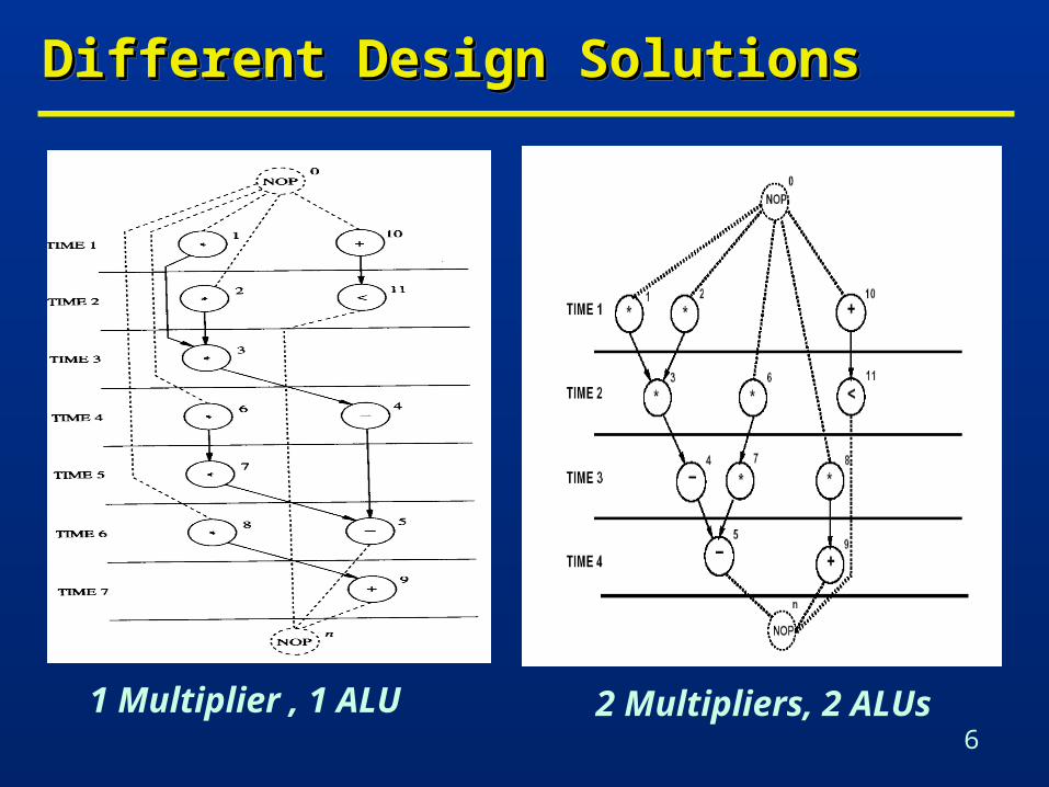
Different Design SolutionsDifferent Design SolutionsDifferent Design SolutionsDifferent Design Solutions
1 Multiplier , 1 ALU 2 Multipliers, 2 ALUs

7
Example of StructuresExample of StructuresExample of StructuresExample of Structures

8
Area vs. Latency TradeoffsArea vs. Latency TradeoffsArea vs. Latency TradeoffsArea vs. Latency Tradeoffs
Multiplier Area: 5Adder Area: 1Other logic Area: 1
9
Architectural-Level Synthesis MotivationArchitectural-Level Synthesis MotivationArchitectural-Level Synthesis MotivationArchitectural-Level Synthesis Motivation
Raise input abstraction level.• Reduce specification of details.
• Extend designer base.
• Self-documenting design specifications.
• Ease modifications and extensions.
Reduce design time. Explore and optimize macroscopic structure
• Series/parallel execution of operations.
Raise input abstraction level.• Reduce specification of details.
• Extend designer base.
• Self-documenting design specifications.
• Ease modifications and extensions.
Reduce design time. Explore and optimize macroscopic structure
• Series/parallel execution of operations.

10
Architectural-Level SynthesisArchitectural-Level SynthesisArchitectural-Level SynthesisArchitectural-Level Synthesis
Translate HDL models into sequencing graphs. Behavioral-level optimization
• Optimize abstract models independently from the implementation parameters.
Architectural synthesis and optimization• Create macroscopic structure
• data-path and control-unit.
• Consider area and delay information of the implementation.

11
Dataflow Graphs …Dataflow Graphs …Dataflow Graphs …Dataflow Graphs …
Behavioral views of architectural models.
Useful to represent data-paths.
Graph• Vertices = operations.
• Edges = dependencies.
Dependencies arise due• Input to an operation is result
of another operation.
• Serialization constraints in specification.
• Two tasks share the same resource.
Behavioral views of architectural models.
Useful to represent data-paths.
Graph• Vertices = operations.
• Edges = dependencies.
Dependencies arise due• Input to an operation is result
of another operation.
• Serialization constraints in specification.
• Two tasks share the same resource.
12
… … Dataflow GraphsDataflow Graphs… … Dataflow GraphsDataflow Graphs
Assumes the existence of variables who store information required and generated by operations.
Each variable has a lifetime which is the interval from birth to death.
Variable birth is the time at which the value is generated.
Variable death is the latest time at which the value is referenced as input to operation.
Values must be preserved during life-time.
13
Sequencing GraphsSequencing GraphsSequencing GraphsSequencing Graphs
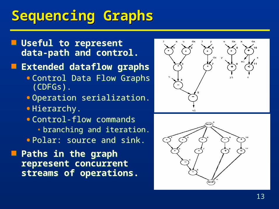
Useful to represent data-path and control.
Extended dataflow graphs• Control Data Flow Graphs
(CDFGs).
• Operation serialization.
• Hierarchy.
• Control-flow commands• branching and iteration.
• Polar: source and sink.
Paths in the graph represent concurrent streams of operations.
Useful to represent data-path and control.
Extended dataflow graphs• Control Data Flow Graphs
(CDFGs).
• Operation serialization.
• Hierarchy.
• Control-flow commands• branching and iteration.
• Polar: source and sink.
Paths in the graph represent concurrent streams of operations.

14
Example of HierarchyExample of HierarchyExample of HierarchyExample of Hierarchy
Two kinds of vertices• Operations• Links: linking sequencing
graph entities in the hierarchy
• Model call• Branching• Iteration
Vertex vi is a predecessor of vertex vj if there is a path with tail vi and head vj
Vertex vi is a successor of vertex vj if there is a path with head vi and tail vj
Two kinds of vertices• Operations• Links: linking sequencing
graph entities in the hierarchy
• Model call• Branching• Iteration
Vertex vi is a predecessor of vertex vj if there is a path with tail vi and head vj
Vertex vi is a successor of vertex vj if there is a path with head vi and tail vj

15
Example of Branching …Example of Branching …Example of Branching …Example of Branching …
Branching modeled by• Branching clause
• Branching body• Set of tasks selected according to value of branching clause.
Several branching bodies• Mutual exclusive execution.
A sequencing graph entity associated with each branch body.
Link vertex models• Branching clause.
• Operation of evaluating clause and taking branch decision.

16
… … Example of BranchingExample of Branching… … Example of BranchingExample of Branching
x= a*b y=x*c z=a+b If (z 0)
• {p=m+n; q=m*n}
x= a*b y=x*c z=a+b If (z 0)
• {p=m+n; q=m*n}

17
Iterative ConstructsIterative ConstructsIterative ConstructsIterative Constructs
Iterative constructs modeled by• Iteration clause
• Iteration body
Iteration body is a set of tasks repeated as long as iteration clause is true.
Iteration modeled through use of hierarchy. Iteration represented as repeated model call to
sequencing graph entity modeling iteration body. Link vertex models the operation of evaluating the
iteration cause.

18
Example of Iteration …Example of Iteration …Example of Iteration …Example of Iteration …

19
… … Example of IterationExample of Iteration… … Example of IterationExample of Iteration
Loop Body

20
Semantics of Sequencing GraphsSemantics of Sequencing GraphsSemantics of Sequencing GraphsSemantics of Sequencing Graphs
Marking of vertices• Waiting for execution.• Executing.• Have completed execution.
Firing an operation means starting its execution. Execution semantics
• An operation can be fired as soon as all its immediate predecessors have completed execution.
Model can be reset by making all operations waiting for execution.
Model can be fired (executed) by firing the source vertex.
Model completes execution when sink completes execution.

21
Vertex AttributesVertex AttributesVertex AttributesVertex Attributes
Area cost. Delay cost
• Propagation delay.
• Execution delay.
Data-dependent execution delays• Bounded (e.g. branching).
• Maximum and minimum delays can be computed• E.g. floating-point data normalization requiring conditional data
alignment.
• Unbounded (e.g. iteration, synchronization).
Area cost. Delay cost
• Propagation delay.
• Execution delay.
Data-dependent execution delays• Bounded (e.g. branching).
• Maximum and minimum delays can be computed• E.g. floating-point data normalization requiring conditional data
alignment.
• Unbounded (e.g. iteration, synchronization).

22
Properties of Sequencing GraphsProperties of Sequencing GraphsProperties of Sequencing GraphsProperties of Sequencing Graphs
Computed by visiting hierarchy bottom-up. Area estimate
• Sum of the area attributes of all vertices.
• Worst-case -- no sharing.
Delay estimate (latency)• Bounded-latency graphs.
• Length of longest path.
Computed by visiting hierarchy bottom-up. Area estimate
• Sum of the area attributes of all vertices.
• Worst-case -- no sharing.
Delay estimate (latency)• Bounded-latency graphs.
• Length of longest path.

23
Compilation and Behavioral OptimizationCompilation and Behavioral OptimizationCompilation and Behavioral OptimizationCompilation and Behavioral Optimization
Software compilation• Compile program into intermediate form.
• Optimize intermediate form.
• Generate target code for an architecture.
Hardware compilation• Compile HDL model into sequencing graph.
• Optimize sequencing graph.
• Generate gate-level interconnection for a cell library.
Software compilation• Compile program into intermediate form.
• Optimize intermediate form.
• Generate target code for an architecture.
Hardware compilation• Compile HDL model into sequencing graph.
• Optimize sequencing graph.
• Generate gate-level interconnection for a cell library.

24
Hardware and Software CompilationHardware and Software CompilationHardware and Software CompilationHardware and Software Compilation
25
CompilationCompilationCompilationCompilation
Front-end• Lexical and syntax analysis.
• Parse-tree generation.
• Macro-expansion.
• Expansion of meta-variables.
Semantic analysis• Data-flow and control-flow analysis.
• Type checking.
• Resolve arithmetic and relational operators.
Front-end• Lexical and syntax analysis.
• Parse-tree generation.
• Macro-expansion.
• Expansion of meta-variables.
Semantic analysis• Data-flow and control-flow analysis.
• Type checking.
• Resolve arithmetic and relational operators.

26
Parse Tree ExampleParse Tree ExampleParse Tree ExampleParse Tree Example
a = p + q * r a = p + q * r
27
Behavioral-Level OptimizationBehavioral-Level OptimizationBehavioral-Level OptimizationBehavioral-Level Optimization
Semantic-preserving transformations aiming at simplifying the model.
Applied to parse-trees or during their generation. Taxonomy
• Data-flow based transformations.
• Control-flow based transformations.
Semantic-preserving transformations aiming at simplifying the model.
Applied to parse-trees or during their generation. Taxonomy
• Data-flow based transformations.
• Control-flow based transformations.

28
Data-Flow Based TransformationsData-Flow Based TransformationsData-Flow Based TransformationsData-Flow Based Transformations
Tree-height reduction. Constant and variable propagation. Common subexpression elimination. Dead-code elimination. Operator-strength reduction. Code motion.
Tree-height reduction. Constant and variable propagation. Common subexpression elimination. Dead-code elimination. Operator-strength reduction. Code motion.

29
Tree-Height ReductionTree-Height ReductionTree-Height ReductionTree-Height Reduction
Applied to arithmetic expressions. Goal
• Split into two-operand expressions to exploit hardware parallelism at best.
Techniques• Balance the expression tree.
• Exploit commutativity, associativity and distributivity.
Applied to arithmetic expressions. Goal
• Split into two-operand expressions to exploit hardware parallelism at best.
Techniques• Balance the expression tree.
• Exploit commutativity, associativity and distributivity.

30
Example of Tree-Height ReductionExample of Tree-Height Reductionusing Commutativity and Associativityusing Commutativity and AssociativityExample of Tree-Height ReductionExample of Tree-Height Reductionusing Commutativity and Associativityusing Commutativity and Associativity
x = a + b * c + d => x = (a + d) + b * c x = a + b * c + d => x = (a + d) + b * c

31
Example of Tree-Height ReductionExample of Tree-Height Reductionusing Distributivityusing DistributivityExample of Tree-Height ReductionExample of Tree-Height Reductionusing Distributivityusing Distributivity
x = a * (b * c * d + e) => x = a * b * c * d + a * e x = a * (b * c * d + e) => x = a * b * c * d + a * e

32
Examples of Propagation & Subexpression Examples of Propagation & Subexpression EliminationEliminationExamples of Propagation & Subexpression Examples of Propagation & Subexpression EliminationElimination
Constant propagation• a = 0; b = a+1; c = 2 * b;
• a = 0; b = 1; c = 2;
Variable propagation• a = x; b = a+1; c = 2 * a;
• a = x; b = x+1; c = 2 * x;
Subexpression elimination• Search isomorphic patterns in the parse trees.
• Example• a = x+y; b = a+1; c = x+y;• a = x+y; b = a+1; c = a;
Constant propagation• a = 0; b = a+1; c = 2 * b;
• a = 0; b = 1; c = 2;
Variable propagation• a = x; b = a+1; c = 2 * a;
• a = x; b = x+1; c = 2 * x;
Subexpression elimination• Search isomorphic patterns in the parse trees.
• Example• a = x+y; b = a+1; c = x+y;• a = x+y; b = a+1; c = a;

33
Examples of Other TransformationsExamples of Other TransformationsExamples of Other TransformationsExamples of Other Transformations
Dead-code elimination• a = x; b = x+1; c = 2 * x;
• a = x; can be removed if not referenced.
Operator-strength reduction• a = x2; b = 3 * x;
• a = x * x; t = x << 1; b = x+t.
Code motion• for (i = 1; i < a * b) { } ;
• t = a * b; for (i = 1; i < t) { }.
Dead-code elimination• a = x; b = x+1; c = 2 * x;
• a = x; can be removed if not referenced.
Operator-strength reduction• a = x2; b = 3 * x;
• a = x * x; t = x << 1; b = x+t.
Code motion• for (i = 1; i < a * b) { } ;
• t = a * b; for (i = 1; i < t) { }.
34
Control-Flow Based TransformationsControl-Flow Based TransformationsControl-Flow Based TransformationsControl-Flow Based Transformations
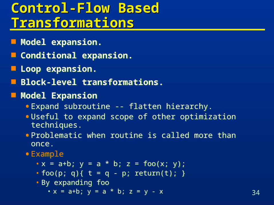
Model expansion. Conditional expansion. Loop expansion. Block-level transformations. Model Expansion
• Expand subroutine -- flatten hierarchy.
• Useful to expand scope of other optimization techniques.
• Problematic when routine is called more than once.
• Example• x = a+b; y = a * b; z = foo(x; y);• foo(p; q){ t = q - p; return(t); }• By expanding foo
• x = a+b; y = a * b; z = y - x

35
Conditional ExpansionConditional ExpansionConditional ExpansionConditional Expansion
Transform conditional into parallel execution with test at the end.
Useful when test depends on late signals. May preclude hardware sharing. Always useful for logic expressions. Example
• If (A>B) { Y= A-B} Else {Y=B-A}.
Example• y = ab; if (a) {x = b + d; } else {x = bd; }
• can be expanded to: x = a (b+d) + a’bd• and simplified as: y = ab; x = y + d (a+b)
36
Loop ExpansionLoop ExpansionLoop ExpansionLoop Expansion
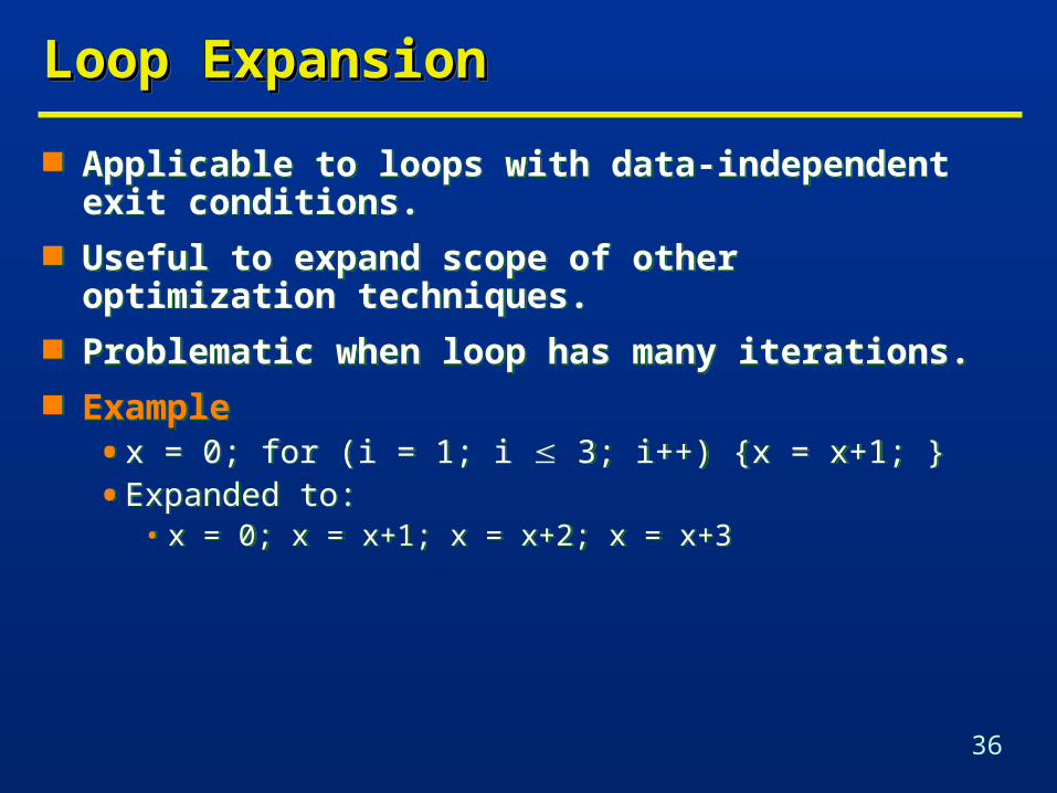
Applicable to loops with data-independent exit conditions.
Useful to expand scope of other optimization techniques.
Problematic when loop has many iterations. Example
• x = 0; for (i = 1; i 3; i++) {x = x+1; }
• Expanded to:• x = 0; x = x+1; x = x+2; x = x+3
Applicable to loops with data-independent exit conditions.
Useful to expand scope of other optimization techniques.
Problematic when loop has many iterations. Example
• x = 0; for (i = 1; i 3; i++) {x = x+1; }
• Expanded to:• x = 0; x = x+1; x = x+2; x = x+3

37
Architectural Synthesis and OptimizationArchitectural Synthesis and OptimizationArchitectural Synthesis and OptimizationArchitectural Synthesis and Optimization
Synthesize macroscopic structure in terms of building-blocks.
Explore area/performance trade-offs• maximum performance implementations subject to area
constraints.
• minimum area implementations subject to performance constraints.
Determine an optimal implementation. Create logic model for data-path and control.

38
Design Space and ObjectivesDesign Space and ObjectivesDesign Space and ObjectivesDesign Space and Objectives
Design space• Set of all feasible implementations.
Implementation parameters• Area.
• Performance• Cycle-time,• Latency,• Throughput (for pipelined implementations).
• Power consumption.
Design space• Set of all feasible implementations.
Implementation parameters• Area.
• Performance• Cycle-time,• Latency,• Throughput (for pipelined implementations).
• Power consumption.

39
Design Evaluation SpaceDesign Evaluation SpaceDesign Evaluation SpaceDesign Evaluation Space

40
Circuit Specification for Architectural Circuit Specification for Architectural SynthesisSynthesisCircuit Specification for Architectural Circuit Specification for Architectural SynthesisSynthesis
Circuit behavior• Sequencing graphs.
Building blocks• Resources.
• Functional resources: process data (e.g. ALU).• Memory resources: store data (e.g. Register).• Interface resources: support data transfer (e.g. MUX and
Buses).
Constraints• Interface constraints
• Format and timing of I/O data transfers.
• Implementation constraints• Timing and resource usage.
• Area• Cycle-time and latency
41
ResourcesResourcesResourcesResources
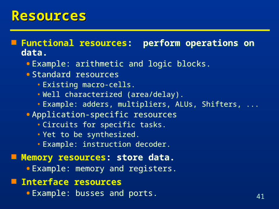
Functional resources: perform operations on data.• Example: arithmetic and logic blocks.
• Standard resources• Existing macro-cells.• Well characterized (area/delay).• Example: adders, multipliers, ALUs, Shifters, ...
• Application-specific resources• Circuits for specific tasks.• Yet to be synthesized.• Example: instruction decoder.
Memory resources: store data.• Example: memory and registers.
Interface resources• Example: busses and ports.
42
Resources and Circuit FamiliesResources and Circuit FamiliesResources and Circuit FamiliesResources and Circuit Families
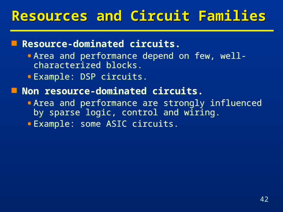
Resource-dominated circuits.• Area and performance depend on few, well-characterized
blocks.
• Example: DSP circuits.
Non resource-dominated circuits.• Area and performance are strongly influenced by sparse
logic, control and wiring.
• Example: some ASIC circuits.
Resource-dominated circuits.• Area and performance depend on few, well-characterized
blocks.
• Example: DSP circuits.
Non resource-dominated circuits.• Area and performance are strongly influenced by sparse
logic, control and wiring.
• Example: some ASIC circuits.

43
Synthesis in the Temporal Domain: Synthesis in the Temporal Domain: SchedulingSchedulingSynthesis in the Temporal Domain: Synthesis in the Temporal Domain: SchedulingScheduling Scheduling
• Associate a start-time with each operation.• Satisfying all the sequencing (timing and resource) constraint.
Goal• Determine area/latency trade-off.• Determine latency and parallelism of the implementation.
Scheduled sequencing graph• Sequencing graph with start-time annotation.
Unconstrained scheduling. Scheduling with timing constraints
• Latency.• Detailed timing constraints.
Scheduling with resource constraints.
Scheduling• Associate a start-time with each operation.• Satisfying all the sequencing (timing and resource) constraint.
Goal• Determine area/latency trade-off.• Determine latency and parallelism of the implementation.
Scheduled sequencing graph• Sequencing graph with start-time annotation.
Unconstrained scheduling. Scheduling with timing constraints
• Latency.• Detailed timing constraints.
Scheduling with resource constraints.
44
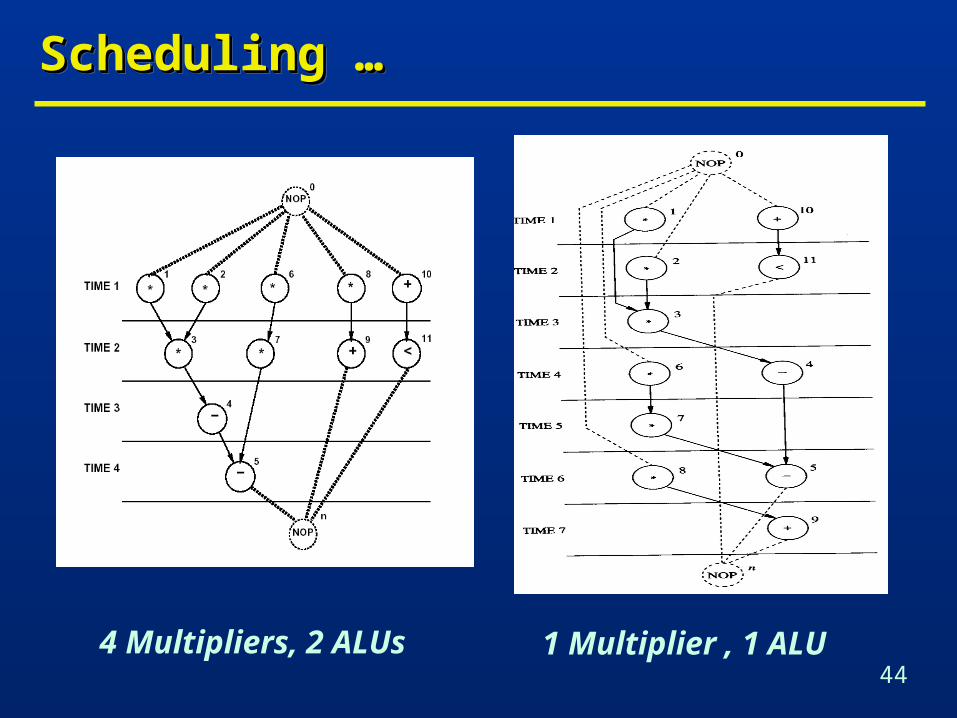
Scheduling …Scheduling …Scheduling …Scheduling …
4 Multipliers, 2 ALUs 1 Multiplier , 1 ALU

45
… … SchedulingScheduling … … SchedulingScheduling
2 Multipliers, 3 ALUs 2 Multipliers, 2 ALUs

46
Synthesis in the Spatial Domain: BindingSynthesis in the Spatial Domain: BindingSynthesis in the Spatial Domain: BindingSynthesis in the Spatial Domain: Binding
Binding• Associate a resource with each operation with the same type.
• Determine area of the implementation.
Sharing• Bind a resource to more than one operation.
• Operations must not execute concurrently.
Bound sequencing graph• Sequencing graph with resource annotation.
Binding• Associate a resource with each operation with the same type.
• Determine area of the implementation.
Sharing• Bind a resource to more than one operation.
• Operations must not execute concurrently.
Bound sequencing graph• Sequencing graph with resource annotation.

47
Example: Bound Sequencing GraphExample: Bound Sequencing GraphExample: Bound Sequencing GraphExample: Bound Sequencing Graph

48
Binding SpecificationBinding SpecificationBinding SpecificationBinding Specification
Mapping from the vertex set to the set of resource instances, for each given type.
Partial binding• Partial mapping, given as
design constraint.
Compatible binding• Binding satisfying the
constraints of the partial binding.
Mapping from the vertex set to the set of resource instances, for each given type.
Partial binding• Partial mapping, given as
design constraint.
Compatible binding• Binding satisfying the
constraints of the partial binding.

49
Performance and Area EstimationPerformance and Area EstimationPerformance and Area EstimationPerformance and Area Estimation
Resource-dominated circuits• Area = sum of the area of the resources bound to the
operations.• Determined by binding.
• Latency = start time of the sink operation (minus start time of the source operation).
• Determined by scheduling
Non resource-dominated circuits• Area also affected by
• registers, steering logic, wiring and control.
• Cycle-time also affected by• steering logic, wiring and (possibly) control.

50
Approaches to Architectural OptimizationApproaches to Architectural OptimizationApproaches to Architectural OptimizationApproaches to Architectural Optimization
Multiple-criteria optimization problem• area, latency, cycle-time.
Determine Pareto optimal points• Implementations such that no other has all parameters with
inferior values.
Draw trade-off curves• discontinuous and highly nonlinear.
Area/latency trade-off• for some values of the cycle-time.
Cycle-time/latency trade-off• for some binding (area).
Area/cycle-time trade-off• for some schedules (latency).

51
Area/Latency Trade-off …Area/Latency Trade-off …Area/Latency Trade-off …Area/Latency Trade-off …
Rationale• Cycle-time dictated by system constraints.
Resource-dominated circuits• Area is determined by resource usage.
General circuits• Area and delay affected by registers, steering logic, wiring and
control logic.• Complex dependency of area and delay on circuit structure.
Scheduling and binding are deeply interrelated.• Most approaches perform scheduling before binding (fits well for
CPU and DSP designs).• Performing binding before scheduling fits control dominated
designs. Approaches
• Schedule for minimum latency under resource constraints.• Schedule for minimum resource usage under latency constraints.

52
… … Area/Latency Trade-offArea/Latency Trade-off… … Area/Latency Trade-offArea/Latency Trade-off
Areas smaller than 20 units. Latency less than 8 cycles. ALU area = 1 unit. MUL area = 5 units. Overhead area = 1 unit. ALU propagation delay 25ns. MUL propagation delay 35 ns. Cycle time = 40 ns
• Resources have unit execution delay.
Cycle time = 30ns
• MUL has 2 unit execution delay.
Areas smaller than 20 units. Latency less than 8 cycles. ALU area = 1 unit. MUL area = 5 units. Overhead area = 1 unit. ALU propagation delay 25ns. MUL propagation delay 35 ns. Cycle time = 40 ns
• Resources have unit execution delay.
Cycle time = 30ns
• MUL has 2 unit execution delay.