coded continuous-phase fsk: information theoretic limits...
TRANSCRIPT

Coded Continuous-phase FSK:
Information Theoretic Limits and Receiver Design
Shi Cheng
Dissertation submitted toCollege of Engineering and Mineral Resources
at West Virginia Universityin partial fulfillment of the requirements for the degree of
Doctor of Philosophyin
Electrical Engineering
Matthew C. Valenti, ChairErdogan Gunel
Daryl S. ReynoldsNatalia A. SchmidBrian D. Woerner
Lane Department of Computer Science and Electrical Engineering
Morgantown,West Virginia2007
Keywords: Orthogonal Modulation, Continuous-phase Frequency ShiftKeying, Error Control Coding, Channel Estimation
c© 2007, Shi Cheng

UMI Number: 3300892
33008922008
UMI MicroformCopyright
All rights reserved. This microform edition is protected against unauthorized copying under Title 17, United States Code.
ProQuest Information and Learning Company 300 North Zeeb Road
P.O. Box 1346 Ann Arbor, MI 48106-1346
by ProQuest Information and Learning Company.
ABSTRACT
Coded Continuous-phase FSK:
Information Theoretic Limits and Receiver Design
Shi Cheng
Continuous-phase frequency shift keying (CPFSK) is a type of frequency shift key-
ing (FSK) that maintains phase continuity from symbol to symbol. The bandwidth
efficiency of a CPFSK waveform is characterized by its modulation index, number of
frequency tones and channel coding rate. These parameters can be flexibly designed to
meet different bandwidth and energy requirements in wireless communication systems.
One special case of CPFSK, orthogonal FSK, could be applied when bandwidth con-
straints are loose. By increasing the number of frequency tones, the energy efficiency
can be improved at the expense of spectral efficiency. In this dissertation, the general
case of orthogonal FSK, orthogonal modulation is first studied. Capacity, convergence
behavior and asymptotic error rates of coded orthogonal modulation are analyzed. In
addition to coherent detection, we consider noncoherent detection as well, which is one
benefit of CPFSK. More often, CPFSK is designed to achieve high spectral efficiency
by reducing its modulation index. The general case of nonorthogonal CPFSK is then
studied. Capacity, spectral efficiency and capacity approaching code design are discussed
for both coherent and noncoherent CPFSK.
In addition to the system design and information theoretic issues, channel estimation
for noncoherent CPFSK is considered. An iterative channel estimation, demodulation
and decoding algorithm is derived using the expectation maximization (EM) algorithm.
Finally, we apply noncoherent CPFSK to frequency hopping (FH) networks, leverag-
ing the results acquired throughout the dissertation. Simulations show FH networks
with CPFSK modulation and channel estimation can achieve robust performance against
partial-band and multiple-access interference.

iii
Acknowledgments
First, I would like to thank Dr. Valenti for offering me the opportunity to study
at West Virginia University and sponsoring my research on wireless communications.
His insightful suggestions are invaluable to my research work, and I enjoyed very much
working for him. Besides, for all my papers and presentations, Dr. Valenti also helped
me a lot, giving me very detailed comments on both technology and English grammar.
He is a terrific advisor and researcher, and I have learned a lot from him.
Next, I would like to thank my committee members for giving assistance to my dis-
sertation work. They are Dr. Erdogan Gunel, Dr. Daryl S. Reynolds, Dr. Natalia A.
Schmid and Brian D. Woerner. I was fortunate to take courses from all of them, which
provides a broad background for my research.
I would also like to give special thanks to Dr. Don Torrieri at U.S. Army Research
Lab. He is one of my major co-authors of several papers, and provided extremely helpful
notes and advices to my research work on CPFSK and frequency hopping networks in
Chapter 4-7.
I would also thank my colleague, Dr. Rohit Iyer Seshadri, for helping verify my results
and comment my papers. Finally, I would like to appreciate my parents for their great
support and encouragement.

Contents
Abstract ii
Acknowledgments iii
List of Tables vii
List of Figures xiii
1 Introduction 1
1.1 Channel Coding . . . . . . . . . . . . . . . . . . . . . . . . . . . . . . . . 1
1.1.1 Linear Block Codes . . . . . . . . . . . . . . . . . . . . . . . . . . 2
1.1.2 Convolutional Codes . . . . . . . . . . . . . . . . . . . . . . . . . 4
1.1.3 Turbo Codes . . . . . . . . . . . . . . . . . . . . . . . . . . . . . 5
1.2 Channel Capacity . . . . . . . . . . . . . . . . . . . . . . . . . . . . . . . 8
1.3 Organization of This Dissertation . . . . . . . . . . . . . . . . . . . . . . 11
2 Coded Orthogonal Modulation 14
2.1 System Model . . . . . . . . . . . . . . . . . . . . . . . . . . . . . . . . . 14
2.1.1 Transmitter . . . . . . . . . . . . . . . . . . . . . . . . . . . . . . 14
2.1.2 Channel and Receiver Front-End . . . . . . . . . . . . . . . . . . 16
2.1.3 Receiver Back-End . . . . . . . . . . . . . . . . . . . . . . . . . . 20
2.2 BICM vs BICM-ID . . . . . . . . . . . . . . . . . . . . . . . . . . . . . . 24
2.2.1 BICM Capacity . . . . . . . . . . . . . . . . . . . . . . . . . . . . 24
2.2.2 Simulation Results . . . . . . . . . . . . . . . . . . . . . . . . . . 26
iv

CONTENTS v
2.2.3 Convergence and Capacity Analysis . . . . . . . . . . . . . . . . . 29
2.3 Chapter Summary . . . . . . . . . . . . . . . . . . . . . . . . . . . . . . 37
3 Asymptotic Analysis of Coded Orthogonal Modulation 38
3.1 Union Bound . . . . . . . . . . . . . . . . . . . . . . . . . . . . . . . . . 40
3.1.1 Joint Inner Code and Modulation Trellis . . . . . . . . . . . . . . 40
3.1.2 Union Bound . . . . . . . . . . . . . . . . . . . . . . . . . . . . . 41
3.2 Pairwise Error Probability . . . . . . . . . . . . . . . . . . . . . . . . . . 48
3.2.1 Coherent Detection . . . . . . . . . . . . . . . . . . . . . . . . . . 48
3.2.2 Noncoherent Detection . . . . . . . . . . . . . . . . . . . . . . . . 49
3.3 Results and Performance Analysis . . . . . . . . . . . . . . . . . . . . . . 52
3.4 Chapter Summary . . . . . . . . . . . . . . . . . . . . . . . . . . . . . . 55
4 Coherent CPFSK 57
4.1 Coherent Detection . . . . . . . . . . . . . . . . . . . . . . . . . . . . . . 59
4.2 Capacity of Coherent Detection . . . . . . . . . . . . . . . . . . . . . . . 61
4.3 Capacity under Spectral Efficiency Constraint . . . . . . . . . . . . . . . 64
4.4 Coded System Implementation . . . . . . . . . . . . . . . . . . . . . . . . 66
4.5 Code Optimization . . . . . . . . . . . . . . . . . . . . . . . . . . . . . . 71
4.5.1 Degree Distribution Optimization . . . . . . . . . . . . . . . . . . 73
4.5.2 Symbol Labeling Issues . . . . . . . . . . . . . . . . . . . . . . . . 74
4.5.3 Interleaver Design Issues . . . . . . . . . . . . . . . . . . . . . . . 76
4.6 Optimization and Simulation Results . . . . . . . . . . . . . . . . . . . . 79
4.7 Chapter Summary . . . . . . . . . . . . . . . . . . . . . . . . . . . . . . 81
5 Noncoherent CPFSK 84
5.1 Capacity of Symbol-by-symbol Noncoherent Detection . . . . . . . . . . 85
5.2 Capacity under Spectral Efficiency Constraint . . . . . . . . . . . . . . . 87
5.3 Multi-symbol Noncoherent Detection . . . . . . . . . . . . . . . . . . . . 93
5.4 Code Design . . . . . . . . . . . . . . . . . . . . . . . . . . . . . . . . . . 95
5.5 Chapter Summary . . . . . . . . . . . . . . . . . . . . . . . . . . . . . . 99

CONTENTS vi
6 Channel Estimation of Noncoherent FSK 100
6.1 Channel Estimator . . . . . . . . . . . . . . . . . . . . . . . . . . . . . . 101
6.1.1 Iterative Decoding, Demodulation and Channel Estimation . . . . 101
6.1.2 EM Channel Estimator . . . . . . . . . . . . . . . . . . . . . . . . 102
6.2 Reduced Complexity Estimation . . . . . . . . . . . . . . . . . . . . . . . 106
6.2.1 Linear Approximation of F (·) . . . . . . . . . . . . . . . . . . . . 106
6.2.2 Hard Limiting of pk,i . . . . . . . . . . . . . . . . . . . . . . . . . 108
6.3 Simulation Results . . . . . . . . . . . . . . . . . . . . . . . . . . . . . . 109
6.4 Complexity Comparison . . . . . . . . . . . . . . . . . . . . . . . . . . . 111
6.5 Chapter Summary . . . . . . . . . . . . . . . . . . . . . . . . . . . . . . 113
7 Application of CPFSK to FH Networks 115
7.1 Frequency Hopping Networks . . . . . . . . . . . . . . . . . . . . . . . . 116
7.2 CPFSK-FH Networks . . . . . . . . . . . . . . . . . . . . . . . . . . . . . 118
7.3 Partial Band Jamming . . . . . . . . . . . . . . . . . . . . . . . . . . . . 120
7.4 Asynchronous Multiple Access Interference . . . . . . . . . . . . . . . . . 123
7.5 Chapter Summary . . . . . . . . . . . . . . . . . . . . . . . . . . . . . . 127
8 Summary and Future Work 128
8.1 Summary . . . . . . . . . . . . . . . . . . . . . . . . . . . . . . . . . . . 128
8.2 Future Work . . . . . . . . . . . . . . . . . . . . . . . . . . . . . . . . . . 130
A Outage Probability of Interference Channels 132
B Minimum Value of Φ∆(δ) of noncoherent detection 134
References 136

List of Tables
2.1 Minimum Eb/N0 required to achieve a BER of 10−5 using the 6138 bit
cdma2000 turbo code, M-ary noncoherent orthogonal modulation, and
either BICM or the proposed BICM-ID technique. The corresponding
Shannon capacities and EXIT thresholds are also given. . . . . . . . . . . 36
4.1 Capacity and code optimization results for spectral efficiency η = 0.5
bps/Hz. The ith element of the labeling vector is the octal value of the bit
pattern labeling symbol qi. The simulation Eb/N0 is the value for which a
system with Nu = 100, 000 message bits and 200 decoder iterations reaches
a simulated BER of 10−5. . . . . . . . . . . . . . . . . . . . . . . . . . . 82
5.1 Optimized codes for MSK at rate r = 0.5. For each of the coherent and
multi-symbol noncoherent (N = 4) detectors, the degree distributions,
capacity, and thresholds are listed. . . . . . . . . . . . . . . . . . . . . . 97
6.1 Number of operations required for each type of estimator to execute one
EM iteration per block of N symbols. M is the modulation order and R
is the number of recursions used to solve (6.16). . . . . . . . . . . . . . . 113
vii

List of Figures
1.1 Convolutional encoders . . . . . . . . . . . . . . . . . . . . . . . . . . . . 5
1.2 Turbo code structure . . . . . . . . . . . . . . . . . . . . . . . . . . . . . 6
1.3 General channel model . . . . . . . . . . . . . . . . . . . . . . . . . . . . 8
1.4 Unconstrained Gaussian capacity vs BPSK capacity . . . . . . . . . . . . 9
1.5 Two dimensional unconstrained capacity vs CM capacities . . . . . . . . 10
2.1 System model diagram . . . . . . . . . . . . . . . . . . . . . . . . . . . . 15
2.2 CM capacity vs BICM capacity of 2 dimensional modulation in AWGN
channel . . . . . . . . . . . . . . . . . . . . . . . . . . . . . . . . . . . . 26
2.3 CM capacity vs BICM capacity for coherent orthogonal modulation in
AWGN channel . . . . . . . . . . . . . . . . . . . . . . . . . . . . . . . . 27
2.4 BER performance in Rayleigh fading (noncoherent detection with CSI) of
the r(o) = 1/4 input-length Nu = 6138 bit cdma2000 turbo code using 64-
ary orthogonal modulation and both BICM (dashed line) and BICM-ID
(solid line). From right to left, the curves show performance after 1, 2, 3,
4, 5, 10, 16, and 30 iterations. . . . . . . . . . . . . . . . . . . . . . . . . 28
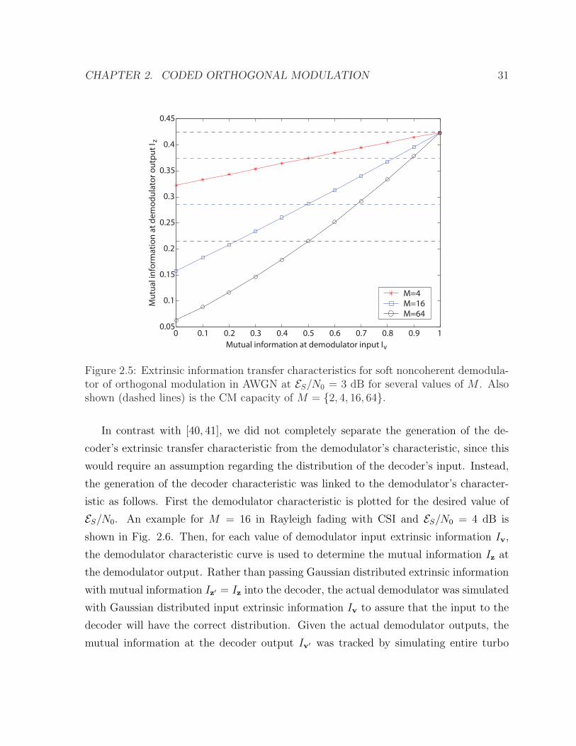
2.5 Extrinsic information transfer characteristics for soft noncoherent demod-
ulator of orthogonal modulation in AWGN at ES/N0 = 3 dB for several
values of M . Also shown (dashed lines) is the CM capacity of M =
{2, 4, 16, 64}. . . . . . . . . . . . . . . . . . . . . . . . . . . . . . . . . . 31
viii

LIST OF FIGURES ix
2.6 EXIT chart for BICM-ID using M = 16 orthogonal modulation and the
rate R = 1/4 length cdma2000 turbo code in Rayleigh fading with nonco-
herent detection CSI at Eb/N0 = 4 dB. Two average decoding trajectories
are shown: The narrower trajectory is for a K = 6138 bit interleaver and
one local channel decoding iteration per global iteration, and the wider tra-
jectory is for a K = 20730 bit interleaver and two local channel decoding
iterations per global iteration. . . . . . . . . . . . . . . . . . . . . . . . . 32
2.7 Minimum Eb/No required to achieve BER = 10−4 and thresholds pre-
dicted by EXIT analysis as a function of code rate R over an AWGN
channel using M-ary orthogonal modulation with noncoherent detection
and the K = 6138 bit cdma2000 turbo code. For M = 2 two points are
shown: The upper point is the simulated value and the lower point is the
EXIT threshold. For M = {4, 16, 64} four points are shown, from top to
bottom: (1) Simulated BICM receiver; (2) Threshold for BICM; (3) Sim-
ulated BICM-ID receiver; and (4) Threshold for BICM-ID. For reference,
the corresponding BICM (dashed) and CM (solid) capacities are shown. . 33
2.8 Minimum Eb/No for a fully interleaved Rayleigh flat-fading channel using
M-ary noncoherent modulation and noncoherent detection with channel
state information. See caption to Fig. 2.7 for full description. . . . . . . 34
2.9 Minimum Eb/No for a fully interleaved Rayleigh flat-fading channel using
M-ary noncoherent modulation and noncoherent detection with no channel
state information. See caption to Fig. 2.7 for full description. . . . . . . 35
3.1 BICM-ID Simulation results of length 6138 turbo coded and convolution-
ally coded orthogonal modulation in AWGN channel, noncoherent detec-
tion. Results shown are up to 20th iteration. . . . . . . . . . . . . . . . . 39
3.2 Trellis merging for the inner code. . . . . . . . . . . . . . . . . . . . . . . 41
3.3 The calculation of tail terminated error events . . . . . . . . . . . . . . . 44
3.4 The concatenation of g(o) = [1 + D4, D + D3 + D4] and g(i) = 1/(1 + D),
with information size Nc = 400 and M = 4, noncoherent reception. The
simulation runs up to 20th iteration. . . . . . . . . . . . . . . . . . . . . . 47

LIST OF FIGURES x
3.5 Bounds of BICOM g(i) = 1 and BICOM-DP g(i) = 1/(1 + D). Both
systems has the outer code g(o) = [1 + D2, 1 + D + D2], 16-ary orthogonal
modulation, fully interleaved Rayleigh fading channel, and noncoherent
Reception with CSI. Simulation results are shown for Nc = 400. The
simulations ran up to 20th iteration. . . . . . . . . . . . . . . . . . . . . . 53
3.6 Bounds of BICOM g(i) = 1 and BICOM-DP g(i) = 1/(1 + D). Both
systems has the outer code g(o) = [1 + D2, 1 + D + D2], 8-ary orthogonal
modulation, AWGN channel, and coherent Reception. Simulation results
are shown for Nc = 600. The simulations ran up to 20th iteration. . . . . 54
3.7 Bounds of BICOM-DP with the outer code g(o) = [1 + D2 + D3, 1 + D +
D2 + D3], 16-ary orthogonal modulation, Nc = 1000. All five channel
reception combinations are shown. . . . . . . . . . . . . . . . . . . . . . 55
3.8 Bounds and simulation results of BICOM and BICOM-DP in AWGN chan-
nel, noncoherent detection . . . . . . . . . . . . . . . . . . . . . . . . . . 56
4.1 Capacities of MSK (M = 2, h = 1/2): From left to right, they are i.u.d.
capacity of coherent detection, i.u.d. capacity of BICM detection and
symbol-wise noncoherent capacity respectively. . . . . . . . . . . . . . . . 64
4.2 Capacities of binary CPFSK for different spectral efficiency constraints.
From top to bottom, the spectral efficiencies are η = 0.75, η = 0.5, η =
0.25 and η = 0.02. h is considered with the denominator up to 5. So from
left to right, they are 15, 1
4, 1
3, 2
5, 1
2, 3
5, 2
3, 3
4and 4
5respectively. Also, the
memoryless orthogonal case h = 1 is listed for reference. . . . . . . . . . 66
4.3 CPFSK capacities of different M for spectral efficiency η = 0.5. h is
considered with the denominator up to 5. So from left to right, they are15, 1
4, 1
3, 2
5, 1
2, 3
5, 2
3, 3
4and 4
5respectively. . . . . . . . . . . . . . . . . . . 67
4.4 Nonsystematic IRA coding structure. “=” corresponds to variable nodes
and “+” corresponds to single parity-check nodes. . . . . . . . . . . . . . 68
4.5 Inner code EXIT curves of M = 4, h = 1/3 with gray and natural label-
ings. Es/N0 = 0dB. . . . . . . . . . . . . . . . . . . . . . . . . . . . . . . 75
4.6 Gray and natural labelings of M = 4, h = 1/3 . . . . . . . . . . . . . . . 76

LIST OF FIGURES xi
4.7 Bad interleaver designs . . . . . . . . . . . . . . . . . . . . . . . . . . . . 77
4.8 Counter example of the lower bound on ρ1 in (4.43) . . . . . . . . . . . . 78
4.9 Optimized EXIT curves for M = 4, h = 1/3 with natural labeling. . . . . 80
4.10 BER of optimized M = 4, h = 1/3 system. The system has uncoded bits
Nu = 100, 000, and the figure shows the BERs of 50,60,70,80,90,100,150
and 200 iterations from top to bottom. . . . . . . . . . . . . . . . . . . . 81
5.1 Capacity of binary CPFSK . . . . . . . . . . . . . . . . . . . . . . . . . . 86
5.2 Minimum Eb/N0 required for noncoherent CPFSK to achieve an arbitrarily
low error rate versus modulation index h in AWGN with M = 2 for several
spectral efficiencies η = {0, 1/3, 1/2, 1}. For fixed h, the minimum Eb/N0
increases with η. . . . . . . . . . . . . . . . . . . . . . . . . . . . . . . . 88
5.3 Minimum Eb/N0 required for noncoherent CPFSK to achieve an arbitrarily
low error rate versus modulation index h in AWGN for several modulation
orders M = {2, 4, 8, 16, 32, 64} and spectral efficiencies η = {0, 1/2}. . . 89
5.4 Minimum Eb/N0 required for noncoherent CPFSK to achieve an arbitrarily
low error rate versus modulation index h in Rayleigh fading for several
modulation orders M = {2, 4, 8, 16, 32, 64} and spectral efficiencies η =
{0, 1/2}. . . . . . . . . . . . . . . . . . . . . . . . . . . . . . . . . . . . . 90
5.5 Minimum Eb/N0 required for noncoherent CPFSK to achieve an arbitrarily
low error rate versus spectral efficiency η in AWGN for several modulation
orders M = {2, 4, 8, 16, 32, 64}. For fixed η the minimum Eb/N0 decreases
with increasing M . The values at η = 0 correspond to the orthogonal FSK
capacity. . . . . . . . . . . . . . . . . . . . . . . . . . . . . . . . . . . . . 91
5.6 Minimum Eb/N0 required for noncoherent CPFSK to achieve an arbitrarily
low error rate versus spectral efficiency η in Rayleigh fading for several
modulation orders M = {2, 4, 8, 16, 32, 64}. For fixed η the minimum
Eb/N0 decreases with increasing M . The values at η = 0 correspond to the
orthogonal FSK capacity. . . . . . . . . . . . . . . . . . . . . . . . . . . . 92
5.7 Capacity of MSK using multi-symbol noncoherent and coherent detection. 95

LIST OF FIGURES xii
5.8 Nonsystematic IRA coding structure. “=” corresponds to variable nodes
and “+” corresponds to single parity-check nodes. . . . . . . . . . . . . . 96
5.9 EXIT curves of inner codes without accumulator . . . . . . . . . . . . . . 97
5.10 EXIT curve-matching result of N = 4 noncoherent detection of MSK . . 98
5.11 BER of MSK with rate r = 0.5 coding designed using EXIT curve-fitting. 98
6.1 F (x) = I1(x)/I0(x) and its linear approximation. . . . . . . . . . . . . . . 107
6.2 BER comparison of the different estimators in block Rayleigh fading with
N = 4 symbols per block. The system uses 16-FSK modulation and the
rate 1/2 cdma2000 turbo code (Nu = 1530 input bits). Shown from left
to right is performance with: (1) a√ES and N0 known for each block; (2)
The full-complexity EM estimator; (3) Estimator EM-H, which makes hard
decisions on pk,i; (4) Estimator EM-L, which uses a linear approximation to
the F (·) function; and (5) Estimator EM-H/L, which makes hard decisions
on pk,i and uses a linear approximation to F (·). . . . . . . . . . . . . . . 110
6.3 Influence of the block length N on the BER performance in block Rayleigh
fading. For each value of N = {4, 8, 16, 32}, two curves are shown. The left
curve (dashed line) shows performance when a√ES and N0 are known for
each block; the right curve (solid line) shows performance with Estimator
EM-H/L. The system uses 16-FSK modulation and the rate 1/2 cdma2000
turbo code (Nu = 1530 input bits). . . . . . . . . . . . . . . . . . . . . . 111
6.4 Performance in AWGN as a function of block length N . The performance
with known ES and N0 (dashed lines) is compared against the performance
with Estimator EM-H/L. Modulation is 16-FSK. The code is the rate 1/2
cdma2000 turbo code with Nu = 1530. . . . . . . . . . . . . . . . . . . . 112
7.1 Throughput Efficiency of FH network in Rayleigh fading environment,
Eb/N0 = 3dB, J = 20 transmitters . . . . . . . . . . . . . . . . . . . . . . 119

LIST OF FIGURES xiii
7.2 Minimum Eb/N0 required for frequency hopping system to achieve BER at
10−3 versus fraction of partial band interference µ, Eb/It0 = 10dB, 32 hops
per codeword, 4-ary CPFSK, h = 0.46, Rayleigh fading, Rician fading
K = 10dB, AWGN channel from top to bottom. UMTS turbo code is
used, with Nu = 2048 information bits and rate r(o) = 16/27. . . . . . . 121
7.3 Minimum Eb/N0 required for frequency hopping system to achieve BER at
10−3 versus fraction of partial band interference µ, Eb/It0 = 10dB, 32 hops
per codeword, 8-ary CPFSK, h = 0.32, Rayleigh fading, Rician fading
K = 10dB, AWGN channel from top to bottom. UMTS turbo code is
used, with Nu = 2048 information bits and rate r(o) = 8/15. . . . . . . . 122
7.4 Minimum Eb/N0 required for frequency hopping system to achieve BER at
10−3 versus fraction of partial band interference µ, Eb/It0 = 13dB, Rayleigh
fading, 4-ary CPFSK(M = 4), h = 0.46, 16,32,64 hops per codeword from
top to bottom. UMTS turbo code is used, with Nu = 2048 information
bits and rate r(o) = 16/27. . . . . . . . . . . . . . . . . . . . . . . . . . . 123
7.5 Minimum Eb/N0 required for frequency hopping system to achieve BER at
10−3 versus fraction of partial band interference µ, Eb/It0 = 13dB, Rayleigh
fading, 8-ary CPFSK(M = 8), h = 0.32, 16,32,64 hops per codeword from
top to bottom. UMTS turbo code is used, with Nu = 2048 information
bits and rate r(o) = 8/15. . . . . . . . . . . . . . . . . . . . . . . . . . . . 124
7.6 Minimum Eb/N0 required for frequency hopping system to achieve BER at
10−4 in multiples access interference, Rayleigh fading, 32 hops per code-
word. UMTS turbo code is used, with Nu = 2048 information bits, rate
r(o) = 1/3 for orthogonal case and r(o) = 16/27 and 8/15 for nonorthogonal
4CPFSK and 8CPFSK respectively. . . . . . . . . . . . . . . . . . . . . . 126
Chapter 1
Introduction
The introduction of turbo codes [1] and rediscovery of low density parity check (LDPC)
codes [2,3] have drawn the attention of the communications research community towards
a deeper understanding of the information theoretic limits of digital communication sys-
tems. These limits include capacity, spectral efficiency and asymptotic performance.
Such information theoretic research provides a benchmark for designing practical sys-
tems, and is important especially for the wireless environment, where the channel is poor
due to severe fading or interference, and the power is limited by the battery.
A practical digital communication system includes channel coding and digital modula-
tion, and their counterparts at the receiver. Modern channel coding, e.g. turbo codes [1]
and LDPC codes [2], can approach the capacity closely. The background of channel
coding is reviewed in Section 1.1. Next the concept of channel capacity is introduced
in Section 1.2. With a capacity-approaching code, the constrained channel capacity is
a more important metric than the uncoded error rate. The modulation constrained ca-
pacity is also discussed in this section. Finally, the organization of the remainder of the
dissertation is given in Section 1.3.
1.1 Channel Coding
Channel coding is a technique that uses redundant information to protect data commu-
nicated through the channel. By encoding the data stream with some redundancy, the
1

CHAPTER 1. INTRODUCTION 2
decoder at the receiver could still possibly recover the data even though the transmission
is corrupted by noise or interference.
In 1948, Shannon’s channel coding theorem [4] stated that if the data rate R is below
the channel capacity C, there exists a way to achieve reliable communications with an
arbitrarily small error probability. Shannon outlined the ideas of the proof in [4], and
the rigorous proof was made much later [5]. The full proofs can now be found in [6] [7],
and they follow the basic idea given by Shannon, using long random codewords. While
the idea of using long random codewords is a useful strategy for proving the theorem,
practical channel coding requires some structure to permit finite complexity encoding
and decoding algorithms.
After the pioneering work by Shannon, there were a lot of contributions in the art of
error control coding. However, practical codes could not approach capacity until Berrou
et al. invented turbo codes in 1993 [1]. Then LDPC codes were reinvestigated [3] using
the idea of iterative decoding from turbo codes, although LDPC codes were first invented
in 1960’s by Gallager [2]. Both turbo codes and LDPC codes are shown to be within 1
dB of the capacity limit.
In the rest of this section, we will introduce linear block codes, convolutional codes
and turbo codes.
1.1.1 Linear Block Codes
A block code is a set of fixed length vectors, whose elements are chosen from an alphabet
of q symbols. When q = 2 and the alphabet has only 0 and 1, the code is said to be
binary. To limit the length and the scope of this dissertation, we will only have a brief
introduction of binary codes here.
If the length of a binary block code is n, there are a total of 2n possible combinations
of the {0, 1} sequence. We may choose a set of 2k, k < n, of them to be the code C. Such
a code is said to have rate R = k/n, usually referred as an (n, k) code. If the modulo 2
sum of any two codewords from C is still in the set, the code is called a linear code. Note
that any codeword added to itself produces all-zeros, which means all linear binary codes
always have the all-zeros codeword. For any two codewords, the Hamming distance is

CHAPTER 1. INTRODUCTION 3
the number of bit positions that differ. For a linear binary code, the minimum Hamming
distance is the minimum Hamming weight (number of ones in a codeword) of all the
codewords except for the all-zeros codeword.
By using linear algebra over the Galois Field GF(2), we can represent the encoding
as,
cT = uTG, (1.1)
where c is a length n column vector representing the coded bits, and u is a length k
column vector representing the uncoded information bits. G is a k × n matrix, called
the generator matrix, whose elements are either 0 or 1. In order to generate 2k distinct
codewords, the rows of G must be linearly independent, which means G needs to be a
full rank matrix or its rows must span a k dimensional subspace of {0, 1}n.
If G has the form of
G = [Ik | P] , (1.2)
the first k bits in c is the same as u. We call such a code a systematic code, the first k
bits of c the systematic bits, and the n− k redundant bit the parity bits.
For any (n, k) linear code, there is always a dual code C⊥ of dimension n − k whose
codewords are orthogoal to all codewords in C. Suppose such a dual code has generator
matrix H of size (n− k)× n. It is easy to see that
GHT = 0, (1.3)
and for any c generated by G,
cTHT = 0. (1.4)
With respect to the (n, k) code, we call H the parity check matrix. For the special case

CHAPTER 1. INTRODUCTION 4
of the systematic code in (1.2), H could be written as
H =[PT | I(n−k)
]. (1.5)
Equation (1.4) plays an important role in decoding. The simplest method is hard
decision decoding. The received vector can be represented as (c+e), where e is the error
vector imposed by the channel. The decoder first finds the syndrome s by multiplying
the received vector by the parity check matrix H,
sT , (c + e)THT = eTHT . (1.6)
Then the decoder looks for the error pattern of e in a predefined table, and then deter-
mines the uncoded information u.
1.1.2 Convolutional Codes
Convolutional codes are encoded by passing the uncoded bits through a finite state shift
register. The encoder for a (n, k, K) convolutional code reads in k bits at a time, passes
the input bits through a shift register with K − 1 stages, and outputs n bits at a time.
K is also called the constraint length of the convolutional code. Fig. 1.1(a) shows
an example of (2,1,4) convolutional code. In order to represent the logic of each tap
associated with each output, we can use generators. The generators in Fig. 1.1(a) can be
written in binary form as g1 = [1011] and g2 = [1101]. Conventionally, we use the octal
form [13,15]. Another way to represent the encoder is the generator polynomial. In this
format, the generator polynomial for the code in Fig. 1.1(a) is [1+D2 +D3, 1+D +D3].
While the two generator polynomials are both feed forward, there is another type
of convolutional code called recursive systematic convolutional (RSC) code, which has
a feedback polynomial. Fig. 1.1(b) shows an example recursive encoder. Basically, the
upper parallel output in 1.1(a) is fed back to the first stage of the shift register. Usually,
we use [1, 15/13] in octal form or the generator polynomials [1, (1+D+D3)/(1+D2+D3)]
to represent the code.
While both codes above have the same codeword set, they have different mapping

CHAPTER 1. INTRODUCTION 5
D D D
g 1
g 2
u
(a) Nonrecursive convolutional encoder
D D D
g 1
g 2
u
(b) Recursive convolutional encoder
Figure 1.1: Convolutional encoders
rules for the encoding. In a nonrecursive code, a single ‘1’ at the input will take the
encoder out of the all zeros state, but the encoder will return to the all-zeros state after
K − 1 consecutive inputs of ‘0’. On the other hand, with a RSC code, the same input
will drive the encoder out of the all-zeros state where it will remain indefinitely, or until
a second ‘1’ is input to the encoder. For this reason, nonrecursive encoders can be
considered to be finite impulse response (FIR) systems, while RSC encoders are infinite
impulse response (IIR) systems.
The Viterbi Algorithm [8] is a widely used algorithm for maximum likelihood sequence
estimation (MLSE), which minimizes the codeword error rate. In recent years, with the
emergence of the turbo codes, the BCJR algorithm [9], which performs maximum a
posteriori (MAP) decoding, has also become widely used.
1.1.3 Turbo Codes
Turbo codes, also called parallel concatenated convolutional codes (PCCC), were intro-
duced by Berrou et al. in 1993 [1]. A turbo encoder is shown in Fig. 1.2(a). The uncoded
bit stream is encoded by the upper recursive convolutional encoder, and the uncoded bits
are bit-wise interleaved and then encoded by the lower recursive convolutional encoder.
The two convolutional encoders could be either identical or different. An optional punc-
turing could be applied on the parity bits from either or both convolutional encoders. In
the case of no puncturing, the turbo encoder will produce one copy of the information

CHAPTER 1. INTRODUCTION 6
bits c(i), one copy of the parity bits from the upper encoder c(u) and one copy of the
parity bits from the lower encoder c(l).
u
Upper Convolutional
Encoder
Lower Convolutional
Encoder
I n t e
r l e a
v e r
c (i)
c (l)
c (u)
(a) Turbo encoder
y
Upper SISO
Lower SISO
D e
i n t e
r l e
a v e
r
z (i)
I n t e
r l e
a v e
r
z e (u) z (u)
z' e (l)
z e (l)
Demodulator
z' e (u)
z' (i)
z' (l)
(b) Turbo decoder
Figure 1.2: Turbo code structure
The turbo decoder is shown in Fig. 1.2(b). It has two soft in soft output (SISO)
convolutional decoders, working in an iterative manner [10]. First, the soft demodulator
calculates the bit-wise log likelihood ratio (LLR) for both information bits and parity
bits. Assuming the modulation is binary and the channel is memoryless, the LLR of xi
is calculated based on the channel observation yi,
zci = logp(yi|ci = 1)
p(yi|ci = 0). (1.7)
Then z(i)c and z
(u)c is then forwarded to the upper SISO decoder. Also, the upper SISO
decoder takes z(l)e from the lower SISO decoder, called extrinsic information, which is the
information that the other component decoder provides for iterative processing. Initially,
the extrinsic information is set to be all-zeros, and it is updated during the decoding, as
we will discuss later. The upper SISO decoder then performs the BCJR algorithm and
produces
z(u)i = log
p(ci = 1|z(i)c , z
(u)c , z
(l)e )
p(ci = 0|z(i)c , z
(u)c , z
(l)e )
. (1.8)
The extrinsic information is calculated by
z(u)e,i = z
(u)i − z
(i)c,i − z
(l)e,i . (1.9)

CHAPTER 1. INTRODUCTION 7
z(u)e is then interleaved to z
′(u)e . Here we use ′ to represent the interleaved copy of the
signal. The lower SISO decoder then takes z′(u)e , z
′(i)c and z
′(l)c to produce
z′(l)i = log
p(ci = 1|z′(i)c , z′(l)c , z
′(u)e )
p(ci = 0|z′(i)c , z′(l)c , z
′(u)e )
. (1.10)
After deinterleaving, if z(l) satisfies a stopping criteria1, the decoding iteration stops and
the hard decision of z(l) is produced as the output. Otherwise, the deinterleaved extrinsic
information of the lower SISO decoder is calculated,
z(l)e,i = z
(l)i − z
(i)c,i − z
(u)e,i . (1.11)
Thus, (1.8), (1.9), (1.10) and (1.11) work in an iterative manner.
Berrou used the same recursive convolutional code [1, 1+D4/1+D+D2+D3+D4] for
both upper and lower encoder in [1], which has a constraint length 5. In this dissertation,
we will use either CDMA2000 turbo code [15] or UMTS turbo code [16] with a lower
constraint length of 4. These two turbo codes have well designed interleavers, and have
a wide range of coding rates and lengths.
CDMA2000 turbo code supports the information sequence length {378, 570, 762,
1146, 1530, 2398, 3066, 4602, 6138, 9210, 12282, 20730} and rate {1/2,1/3,1/4,1/5}. It
uses a pair of rate 1/3 recursive systematic convolutional constituent codes with generator
polynomials [1, (1 + D + D3)/(1 + D2 + D3), (1 + D + D2 + D3)/(1 + D2 + D3)]. The
unpunctured rate of the code is 1/5. Rate 1/4 is achieved by puncturing every other bit
in the second parity stream; rate 1/3 is achieved by puncturing the entire second parity
stream; rate 1/2 is achieved by puncturing the entire second parity stream and every
other bit in the first parity stream.
UMTS turbo code supports any information sequence length from 40 to 5114. It has
the same constituent encoders as the one in Fig. 1.1(b), which is the same as CDMA2000
turbo code at rate 1/3. The base rate of the UMTS code is 1/3, but the standard also
1Different stopping criteria for turbo decoding are studied in [11–14]. Among these stopping criteria,cross entropy check is based on the soft output of the decoder, while sign check and cyclic redundancycheck (CRC) is based on the hard decision output. In this dissertation, we assume perfect CRC, i.e. thecomplexity and the error rate induced by CRC are zero.

CHAPTER 1. INTRODUCTION 8
EncoderChannelp(Y|X)
Decoder
X Y
Figure 1.3: General channel model
has a rate matching procedure which supports any rate above 1/3.
1.2 Channel Capacity
A general channel model is shown in Fig. 1.3. It has input X and output Y , and can be
modelled by its transition probability p(Y |X). The capacity of the channel is defined as
C , maxp(x)
I(X; Y ), (1.12)
where I(X; Y ), the mutual information between X and Y , is defined as
I(X; Y ) , E
[log
p(X, Y )
p(X)p(Y )
], (1.13)
and the maximization in (1.12) is taken over all possible input distributions p(x).
A simple but widely used channel model is the Additive White Gaussian Noise
(AWGN) channel. Under the input signal average power constraint E(X2) 6 ES, the
capacity is
C =1
2log2
(1 +
2ES
N0
)bits/channel use, (1.14)
where N0 is the one sided noise spectral density of the channel. By Shannon’s channel
coding theorem, any data rate R 6 C is achievable, and conversely, it is not possible for
any rate R > C to be supported with an arbitrarily low error probability [4]. Equation
(1.14) is achieved by choosing X to be Gaussian distributed with zero mean and variance
ES. In this case, X has an infinite alphabet size. Since there is no other constraint on X
except for the power constraint, we call this capacity C the unconstrained capacity.

CHAPTER 1. INTRODUCTION 9
Es/No(dB)
C a p
a c i t y
( b i
t s )
-15 -10 -5 0 5 10 15 20 0
0.5
1
1.5
Unconstrained Gaussian Capacity CM Capacity: BPSK
Figure 1.4: Unconstrained Gaussian capacity vs BPSK capacity
However, the Gaussian input pdf for X is not feasible due to its infinite alphabet
size and unbounded instantaneous power maxX2. Instead, in practical communication
system, X must be chosen from a finite alphabet X . This selection process is called
modulation, and X is the constellation of the modulation. When the source is appropri-
ately encoded, each constellation point will occur with equal probability. Therefore, the
channel capacity under modulation constraints can be written as
C = log2 |X | − E
[log2
∑|X |−1k=0 p(Y |Xk)
p(Y |X)
], (1.15)
where |X | is the cardinality of X . Usually, (1.15) does not have a closed form solu-
tion when the expectation involves a multi-dimensional integral. Instead, Monte-Carlo
integration can be used to find a numerical solution.
Fig. 1.4 shows the unconstrained Gaussian channel capacity and binary phase shift
keying (BPSK) constrained capacity. Note that the unconstrained capacity is always

CHAPTER 1. INTRODUCTION 10
Es/No(dB)
C a p
a c i t
y ( b
i t s )
-10 -5 0 5 10 15 20 25 30 0
0.5
1
1.5
2
2.5
3
3.5
4
4.5
5 Unconstrained Gaussian Capacity CM Capacity 16QAM CM Capacity 8PSK CM Capacity 4PSK CM Capacity BPSK
Figure 1.5: Two dimensional unconstrained capacity vs CM capacities
higher than the BPSK capacity. At low ES/N0, the two capacities are very close. But
when ES/N0 becomes greater than 5 dB, the BPSK capacity reaches a limit of one
bit per channel use, which is the base 2 log of the cardinality of X = {−√ES,√ES}.
In order to achieve the BPSK capacity and other modulation constrained capacities, a
capacity-approaching channel coding is usually necessary. So we also call this constella-
tion constrained capacity the coded modulation (CM) capacity. For a fixed constellation,
the CM capacity serves as a benchmark for the performance of the coded system.
In modern digital communications, the modulation is allowed to span multiple dimen-
sions. Given a complex domain, the unconstrained capacity of Gaussian channels can be
achieved by distributing equal energy on each dimension. Thus, the real and imaginary
dimensions each have the capacity in (1.14) with half energy. Therefore,
C = log2
(1 +
ES
N0
). (1.16)
In Fig. 1.5, we show this unconstrained complex Gaussian channel capacity and the

CHAPTER 1. INTRODUCTION 11
constrained capacities of some two dimensional modulations, including 4-ary and 8-ary
phase shift keying (PSK) and 16-ary quadrature amplitude modulation (QAM). PSK
uses the phase to carry information, and its constellation is
XPSK = {√ESe
j2πkM , k = 0, 1, · · · ,M − 1}. (1.17)
QAM carries the information on the amplitudes of both dimensions. The constellation
of a square QAM, i.e.√
M is an integer, can be represented as,
XQAM =
{η
(kI −
√M − 1
2
)+ η
(kQ −
√M − 1
2
)j, kI , kQ = 0, 1, · · · ,
√M − 1
}
. (1.18)
where η is the normalization constant to meet the constraint E(X2) ≤ ES.
It is seen that (1.16) is an upper bound on the constrained capacities of all types of
two dimensional modulation. When the ES/N0 is high enough, the capacities with finite
constellation all reach the limit of log2 |X |.We have considered the AWGN channel and compared the unconstrained capacity
with the modulation constrained capacities. In this dissertation, we will consider M-
ary orthogonal modulation and nonorthogonal frequency shift keying (FSK), and also
consider some other types of channels, e.g. ergodic fading channel and block fading
channel, which will be introduced in the next chapter.
1.3 Organization of This Dissertation
In this chapter, we gave a brief background on channel coding and channel capacity. The
rest of this dissertation consists of three parts. The first part is Chapter 2 and Chapter 3,
which covers the information theoretic limits of coded orthogonal modulation. Chapter
2 focuses on the capacity of orthogonal modulation; and it is demonstrated that iterative
demodulation and decoding is beneficial for systems with coded orthogonal modulation.
In Chapter 3, the asymptotic error rate is analyzed for convolutional coded orthogonal
modulation system. A recursive inner code structure is used to exploit the interleaving

CHAPTER 1. INTRODUCTION 12
gain in frame error rate.
The second part of the dissertation includes Chapter 4 and Chapter 5, which mainly
focus on the information theoretic limits of nonorthogonal modulation. In particular,
nonorthogonal continuous phase frequency shift keying (CPFSK) is considered because
of its compact bandwidth. Chapter 4 studies the coherent CPFSK detector for AWGN.
By treating CPFSK and AWGN as a finite state Markov channel (FSMC), the identically
uniformly distributed (i.u.d.) capacities are evaluated through Monte Carlo simulation.
Then the capacity under spectral efficiency constraints are analyzed, and a code design
method to approach the evaluated capacity is also introduced in this chapter. Next,
in Chapter 5, we turn our attention to noncoherent detection. First, the capacity of
symbol-by-symbol noncoherently detected CPFSK is evaluated, and then the capacity
under spectral efficiency constraints is discussed. Then, in AWGN, the multi-symbol
noncoherent detector is analyzed, which achieves the coherent capacity when the block
size is large enough. The design of capacity approaching codes is also covered at the end
of this chapter.
The last part of the dissertation considers other issues related to noncoherent CPFSK.
Chapter 6 derives the channel estimator for noncoherent CPFSK using a priori informa-
tion from the decoder. The estimator uses the expectation maximization (EM) algorithm,
and works jointly with the demodulator and decoder. Next, nonorthogonal noncoherent
CPFSK is applied to frequency hopping (FH) networks in Chapter 7. Simulation results
show good performance against both partial band jamming and multiple access interfer-
ence. Finally, the summary of this dissertation and a few open problems for future work
are addressed in Chapter 8.
The work in this dissertation has been externally published. In particular, the capac-
ity of noncoherent orthogonal modulation and the convergence behavior of coded system
in Chapter 2 are presented in [17, 18]. [19] includes the asymptotic analysis of coded
orthogonal modulation system in Chapter 3. The capacity and code design of coherent
and multi-symbol noncoherent CPFSK in Chapter 4 and 5 appear in [20]. Chapter 4
also refers to the BICM coherent capacity published in [21]. The capacity of symbol-by-
symbol noncoherent CPFSK is presented in [22]. The channel estimator for noncoherent
orthogonal FSK in Chapter 6 is presented in [23,24]. It is straightforward to be extended

CHAPTER 1. INTRODUCTION 13
to nonorthogonal CPFSK, and its application to FH networks in Chapter 7 appears
in [25, 26]. Other related publications but not covered in this dissertation include [27]
and [28]. [27] discussed the throughput of a macrodiversity network, and the duo binary
turbo codes for digital video broadcasting (DVB) are described in [28].

Chapter 2
Coded Orthogonal Modulation
In this chapter, a general system model for coded orthogonal modulation is given. The
system uses a pragmatic approach to coded modulation known as bit interleaved coded
modulation (BICM) [29]. We show from capacity and error rate simulations that iterative
demodulation and decoding is desirable for orthogonal modulation. This is called bit in-
terleaved coded modulation with iterative decoding (BICM-ID) [30,31]. The convergence
behavior of BICM-ID is also considered in this chapter.
In the following discussion, bold lowercase letters will be used to denote (column)
vectors, e.g. x, and bold uppercase will be used for matrices, e.g. X. The scalar value
xi,j is used to denote the (i, j)th entry of the matrix X, while the scalar value xi is used
to denote the ith element of the vector x. All matrices and vectors are indexed starting
at zero, x = [x0, x1, ..., xM−1]T . Matrices may be represented as a row of column vectors,
e.g. X = [x0,x1, ...,xN−1].
2.1 System Model
2.1.1 Transmitter
As shown in Fig. 2.1, a vector u ∈ {0, 1}Nu of message bits is passed through an outer
rate r(o) = k(o)/n(o) binary encoder to produce a codeword c′ ∈ {0, 1}Nc . The codeword
is passed through an interleaver, which permutes the order of the code bits. The output
14

CHAPTER 2. CODED ORTHOGONAL MODULATION 15
OuterEncoder
u c’ c X
Π
InnerEncoder
M-aryOrthogonalModulator
H
N
Inner SISO &Demapper
Y1−Π
Π
OuterSISO
k / n(i) (i)k / n(o) (o)ES
zz’
v’ v
u
Serial/Parallel
Converter
DemodulatorS
b B
NoncoherentChannel
Estimator
N0 E Sa
Figure 2.1: System model diagram
of the interleaver c is then optionally encoded by the inner rate r(i) = k(i)/n(i) binary
encoder to generate a codeword b′ ∈ {0, 1}Nb , where r(i) = 1 when the inner encoder is
not present. The lengths of the codewords have the following relationship,
Nc = Nun(o)/k(o) + N
(o)t (2.1)
Nb = Ncn(i)/k(i) + N
(i)t , (2.2)
where N(o)t and N
(i)t are the number of coded tail bits appended by the outer and inner
encoder respectively. In Chapter 2 and 3, the outer code could be a convolutional code
or a turbo code. In this chapter, we first consider operation without an inner encoder,
i.e. b = c, and then in Chapter 3 we introduce the recursive structure to achieve lower
asymptotic error bound.
After the binary encoding by both encoders, the sequence b is forwarded into the
serial to parallel converter, which reshapes the sequence into a matrix B with m = log2 M
rows and Nq columns. It is assumed that Nb = mNq, which can be accomplished by zero
padding when Nq does not divide Nq. The ith column of B represents the bits to be
sent during the ith signaling interval. The binary matrix B is then transformed into a

CHAPTER 2. CODED ORTHOGONAL MODULATION 16
length-Nq vector q with elements from the set {0, 1, ..., M − 1}. The ith element of q is
found from the m code bits in the ith column of B by the natural mapping
qi =m−1∑
k=0
2kbk,i. (2.3)
The memoryless orthogonal modulator then uses the vector q to form the modulated
symbol matrix X =[x0,x1, · · · ,xNq−1
], with each symbol picked from the orthogonal
set X = {e0, e1, · · · , eM−1} of elementary column vectors1. Without loss of generality,
we assume xi = eqi. In orthogonal FSK, q is the sequence of tones to be transmitted.
Note that because of symmetry of orthogonal modulation, natural mapping is equivalent
to any other type of mapping.
2.1.2 Channel and Receiver Front-End
The modulated signal passes through a frequency-nonselective fading channel with addi-
tive Gaussian noise. The receiver front-end downconverts the signal and passes it through
a bank of 2M matched filters (or correlators), a quadrature pair for each of the M pos-
sible transmitted tones [32, 33]. The output of the matched filters are sampled at the
symbol rate and each quadrature pair is represented as a complex scalar value. The
complex samples are then placed into an M ×Nq matrix Y whose ith column represents
the outputs of the matched filters corresponding to the ith received symbol. Note that
we assume perfect symbol synchronization.
Block Fading Channel
We assume the channel is a block-fading channel, which means that the channel is cor-
related in such a way that blocks of N contiguous symbols experience the same fading
amplitude, though each symbol in the block could experience different phase shifts. An
appropriate choice for N is to equate it to the coherence time of the channel [34]. Fur-
thermore, it is assumed that while the noise spectral density is constant for the duration
of a block, it could vary from one block to the next in an arbitrary manner.
1ek is all zeros except for a one in position k.

CHAPTER 2. CODED ORTHOGONAL MODULATION 17
If there are N symbols per block, then there will be L = dNq/Ne blocks per codeword.
The matrix Y can be partitioned according to Y = [Y0,Y1, ...,YL−1], where the M by N
submatrix Y` contains the received signal vectors corresponding to the `th fading block.
The complex channel gain during the `th block can be represented by the N×N diagonal
matrix
H` = a`diag(ejθ0,` , . . . , ejθN−1,`
)(2.4)
where j =√−1, a` is the (real-valued) fading amplitude during the `th block. θi,` is the
random phase shift on the ith symbol, which could be caused by fading and oscillator
phase noise. In this dissertation, we assume that a` is a random Rician variable with
factor K, which has the pdf
p(a) =a
σ2R
e−x2+m2
R2σ2
R I0
(mRx
σ2R
), (2.5)
where
mR =
√K
K + 1(2.6)
σ2R =
1
2(K + 1), (2.7)
and Iµ in (2.5) is the modified Bessel function of the first kind and order µ.
The `th block at the output of the receiver front-end is then
Y` =√ESX`H` + N`, (2.8)
where X` consists of the corresponding columns of X and N` is a M × N noise matrix
whose elements are independently and identically distributed (i.i.d.) complex Gaussian
variables that have independent real and imaginary components with zero mean and
variance N0,`/2.

CHAPTER 2. CODED ORTHOGONAL MODULATION 18
Combining all the blocks together, we can get
Y =√ESXH + N, (2.9)
where
H =
H0
H1
. . .
HL−1
. (2.10)
A special case is when the number of symbols per block is N = 1, and the noise spectral
density is constant over the whole codeword. In this case, each symbol is subject to i.i.d
fading, and we call this ergodic fading, or fully interleaved fading.
Furthermore, if we let the Rician fading factor K be zero, the channel becomes a
Rayleigh fading channel. If we let the Rician fading factor K be infinity, all the fad-
ing amplitude will equal unity, which is the same as with an AWGN channel except
for the random phase. For the coherent detector with known phase information, this
channel is equivalent to the AWGN channel. If the detector is noncoherent, the phase is
marginalized out of the decision variable, as discussed below.
Coherent Detection
The demodulator can perform coherent detection if the fading amplitude a and phase θ
is known to the receiver. Let’s drop the block index `. With knowledge of the symbol
energy ES and the noise spectral density N0, we can represent the conditional pdf of the
(k, i)th entry of Y given that the transmitted symbol is qi = ν, as
p(yk,i|qi = ν, aejθ, ES, N0) =1
πN0
exp
(−
∣∣yk,i − aejθ√ESδk,ν
∣∣2N0
), (2.11)

CHAPTER 2. CODED ORTHOGONAL MODULATION 19
where δk,ν is the Kroneker delta function (δk,ν = 1 if k = ν, otherwise δk,ν = 0). Therefore,
the pdf of yi given qi = ν is
p(yi|qi = ν, aejθ, ES, N0)
=
(1
πN0
)M
exp
(−
∑M−1k=0 |yk,i|2 + a2ES
N0
)exp
(2√ESReal(a−jθyν,i)
N0
). (2.12)
Cancelling out the terms common to all ν, the symbol-wise likelihood can be computed
using only the final exponential factor.
Noncoherent Detection
Based on the coherent metric (2.12), we can derive the noncoherent detector when the
phase information is missing. In this case, we can still make use of the known amplitude
information, and we call this noncoherent detection with channel state information (CSI).
To compute the conditional probability without phase, we can take the expectation of
(2.12) over the random phase θ, which is assumed to be i.i.d. uniform over the range
[0, 2π). As a result, we get
p(yi|qi = ν, a, ES, N0)
=
∫
θ
p(yi|qi = ν, aejθ, ES, N0)p(θ)dθ
=
(1
πN0
)M
exp
(−
∑M−1k=0 |yk,i|2 + a2ES
N0
)I0
(2a√ES|yν,i|
N0
), (2.13)
Again, the only term in (2.13) dependent upon ν is the final factor, which is computed
in the demodulator as the symbol-wise likelihood.
Another type of noncoherent detector operates without CSI, when neither fading
amplitude nor phase information is known to the receiver. However, even though the
instantaneous fading information is unknown, the detector does know the fading statistics
information, for instance that the fading is Rician fading with a particular K factor.
Integrating over the phase θ and fading amplitude a, we get the conditional pdf of yk,i

CHAPTER 2. CODED ORTHOGONAL MODULATION 20
given qi = ν,
p(yk,i|qi = ν, ES, N0)
=
1
π(N0+ES
K+1)exp
(−|yk,i|2+ K
K+1ES
N0+ES
K+1
)I0
(2√
KK+1
√ES|yk,i|N0+
ESK+1
)k = ν
1πN0
exp
(−|yk,i|2
N0
)k 6= ν
(2.14)
Thus, the pdf for the ith symbol is
p(yi|qi = ν, ES, N0) ∝ exp
(ES |yν,i|2
N0((K + 1)N0 + ES)
)I0
(2√
K(K + 1)ES |yν,i|(K + 1)N0 + ES
)
, (2.15)
where A ∝ B means A is proportional to B. When K = 0, (2.15) reduces to
p(yi|qi = ν, ES/N0) ∝ exp
( ES
N0|yν,i|2
ES
N0+ 1
)(2.16)
which is the noncoherent noCSI metric for the Rayleigh fading channel.
When neither the instantaneous fading coefficient nor the fading statistics are known,
channel estimation is performed to estimate the parameters needed by the noncoherent
CSI metric in (2.13), namely A , N0 and B , 2a√ES. The estimator works in the joint
manner together with the decoder. We will introduce this channel estimator in Chapter
6.
After all possible symbol-wise likelihoods are calculated, they form the matrix S,
whose νth row and ith column’s element is defined as sν,i , p(yi|qi = ν).
2.1.3 Receiver Back-End
The symbol-wise likelihood matrix S, computed by the demodulator based on the channel
observation matrix Y, is passed to the receiver back-end, which comprises three main
processing modules: a channel estimator, an inner soft-input/soft-output (SISO) decoder

CHAPTER 2. CODED ORTHOGONAL MODULATION 21
[35] and outer decoder. To simplify the discussion below, we now only consider the
demodulator without the noncoherent channel estimator, which produces the likelihoods
of (2.12), (2.13) or (2.15), depending on what channel state information is known to the
demodulator. The details of the noncoherent channel estimator can be found in Chapter
6. For the remainder of this chapter, we consider no inner encoder in the transmitter,
which drives the inner SISO decoder to be an M-ary demapper.
BICM Receiver
The demapper is the back-end of the demodulator. In the absence of feedback from the
decoder, it transforms the symbol-wise likelihoods S into a m by Nq matrix Z whose
(k, i)th element is the log-likelihood ratio (LLR)
zk,i = logp(bk,i = 1|yi)
p(bk,i = 0|yi)
= log
∑q∈Q(1)
kp(yi|q)∑
q∈Q(0)k
p(yi|q) , (2.17)
where Q(b)k contains all the symbols 0, 1, ...,M − 1 labelled with bk = b. The second
equality of (2.17) comes from Bayes rule and the equally likely symbols. The matrix Z
is reshaped into a length Nb vector and deinterleaved, and the resulting vector z′ is fed
into the outer decoder.
BICM-ID Receiver
If the outer SISO decoder is used, its soft output can be fed back to the demapper
for iterative processing. The extrinsic information v′ at the output of the decoder is
interleaved and reshaped into a m by Nq matrix V containing the a priori information
vk,i = logp(bk,i = 1|Z\zk,i)
p(bk,i = 0|Z\zk,i). (2.18)
Conditioning on Z\zk,i means that the extrinsic information for bit bk,i is produced
without using zk,i.

CHAPTER 2. CODED ORTHOGONAL MODULATION 22
When V is fed back to the demapper, the output (2.17) is replaced by the extrinsic
information
zk,i = logp(bk,i = 1|yi,vi\vk,i)
p(bk,i = 0|yi,vi\vk,i)
= log
∑q∈Q(1)
kp(q|yi,vi\vk,i)∑
q∈Q(0)k
p(q|yi,vi\vk,i). (2.19)
Now consider how the summand in (2.19) can be computed. First, using Bayes’ rule
p(q|y,v\vk) =p(y|q,v\vk)p(q,v\vk)
p(y,v\vk). (2.20)
After conditioning on q, y is independent of v and thus p(y|q,v\vk) = p(y|q). From the
definition of conditional probability, p(q,v\vk) = p(q|v\vk)p(v\vk). Gathering all these
factors, we obtain
p(q|y,v\vk) =p(y|d)p(q|v\vk)p(v\vk)
p(y,v\vk). (2.21)
Inserting this back into (2.19) and cancelling common factors yields
zk,i = log
∑q∈Q(1)
kp(yi|q)p(q|vi\vk,i)∑
q∈Q(0)k
p(yi|q)p(q|vi\vk,i). (2.22)
The contribution of the a priori information is passed to the demapper from the decoder,
which affects only the p(q|v\vk) term. Under the assumption of independent code bits
(achieved by proper interleaving), the probability of q given the a priori input v is
p(q|v) =m−1∏j=0
p(bj(q)|vj), (2.23)
where bj(q) is the value of the jth bit in the labelling of symbol q, which can be found for
j = {0, ..., m− 1} by inverting (2.3). The a priori input is interpreted by the demapper
to be v = log[p/(1− p)], where p is the decoder’s most recent estimate of the probability

CHAPTER 2. CODED ORTHOGONAL MODULATION 23
that the corresponding code bit is a one. Inverting the logarithm and solving for p yields
p = ev/(1 + ev), which the demapper uses for p(b = 1|v). Similarly, the demapper uses
1− p = 1/(1 + ev) for p(b = 0|v). Since b = {0, 1}, the following expression can be used
for both cases:
p(b|v) =ebv
1 + ev. (2.24)
Substituting (2.24) into (2.23) yields
p(q|v) =m−1∏j=0
evjbj(q)
1 + evj. (2.25)
The term p(q|v\vk) in (2.22) is only computed for those q ∈ Q(b)k , in which case p(bk =
b|v\vk) = p(bk = b) = 1/2. Thus,
p(q|v\vk) =1
2
m−1∏j=0j 6=k
evjbj(q)
1 + evj, q ∈ Q(b)
k (2.26)
and indeed vk is not used in this calculation.
The soft demapper output zk is found by substituting (2.26) into (2.22). Since (2.22)
contains a ratio of probabilities, several factors cancel, such as the denominator of (2.26).
Thus,
zk,i = log
∑
q∈Q(1)k
p(yi|q)m−1∏j=0j 6=k
exp (bj(q)vj,i)
∑
q∈Q(0)k
p(yi|q)m−1∏j=0j 6=k
exp (bj(q)vj,i)
, (2.27)
where p(yi) is calculated by (2.12), (2.13) or (2.15). Note that (2.12) has a convenient
exponential form, while (2.13) and (2.15) both have the Bessel function term. If we
further define the combination of log and Bessel function, log I0(·), we can calculate

CHAPTER 2. CODED ORTHOGONAL MODULATION 24
(2.27) in log domain. Therefore,
zk,i = max∗q∈Q(1)
k
log p(yi|q) +
m−1∑j=0j 6=k
bj(q)vj,i
−max∗
q∈Q(0)k
log p(yi|q) +
m−1∑j=0j 6=k
bj(q)vj,i
.(2.28)
where the pairwise max-star operator is defined in [36], max∗(x, y) = max(x, y)+ log(1+
e−|x−y|) = max(x, y) + fc(|x− y|), and for multiple arguments,
max∗i
{xi} = log
{∑i
exi
}. (2.29)
After (2.28) is computed, it is forwarded to the outer SISO decoder again. Thus the
demapper and decoder work in an iterative manner, with binary extrinsic information
exchanged between them.
2.2 BICM vs BICM-ID
In [29], Caire showed that the capacity of BICM with gray labelling approaches the CM
capacities. Gray labelling is the labelling such that for any constellation point X, no more
than one closest neighbor can have the the same bit on any position where X differs. For
many 2-Dimensional constellations, e.g. M-ary QAM and PSK, a gray labelling exists.
However, when the constellation is not gray labelled, a gap can always be found between
the BICM capacity and the CM capacity, which leads to a performance loss in an actual
coded system.
2.2.1 BICM Capacity
The BICM capacity [29] is defined as the mutual information between the modulator
input and the output of the demapper without the feedback from the outer decoder.
Let us use B to denote a random variable in the sequence b, and use Z to denote
the corresponding variable in z, calculated from (2.17) without the feedback from the
CHAPTER 2. CODED ORTHOGONAL MODULATION 25
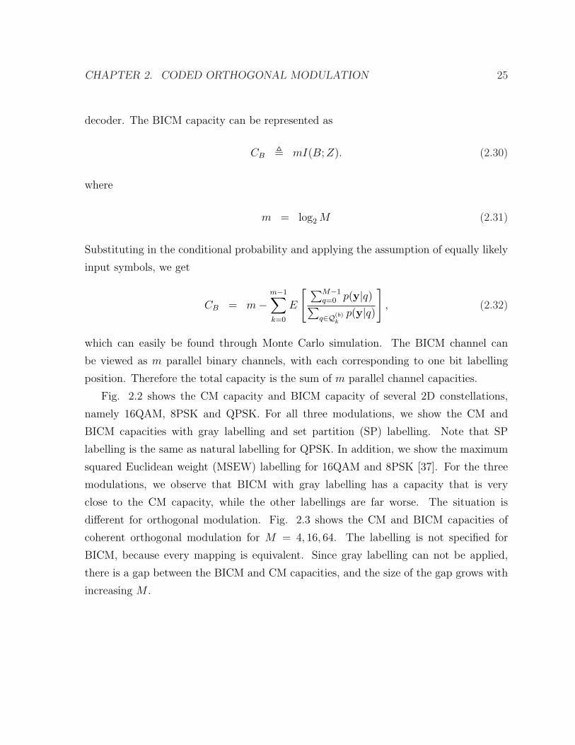
decoder. The BICM capacity can be represented as
CB , mI(B; Z). (2.30)
where
m = log2 M (2.31)
Substituting in the conditional probability and applying the assumption of equally likely
input symbols, we get
CB = m−m−1∑
k=0
E
[ ∑M−1q=0 p(y|q)∑
q∈Q(b)k
p(y|q)
], (2.32)
which can easily be found through Monte Carlo simulation. The BICM channel can
be viewed as m parallel binary channels, with each corresponding to one bit labelling
position. Therefore the total capacity is the sum of m parallel channel capacities.
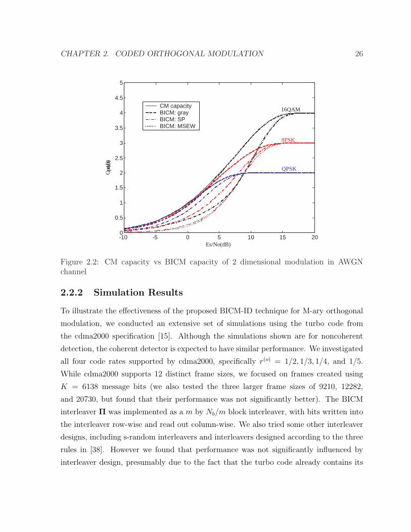
Fig. 2.2 shows the CM capacity and BICM capacity of several 2D constellations,
namely 16QAM, 8PSK and QPSK. For all three modulations, we show the CM and
BICM capacities with gray labelling and set partition (SP) labelling. Note that SP
labelling is the same as natural labelling for QPSK. In addition, we show the maximum
squared Euclidean weight (MSEW) labelling for 16QAM and 8PSK [37]. For the three
modulations, we observe that BICM with gray labelling has a capacity that is very
close to the CM capacity, while the other labellings are far worse. The situation is
different for orthogonal modulation. Fig. 2.3 shows the CM and BICM capacities of
coherent orthogonal modulation for M = 4, 16, 64. The labelling is not specified for
BICM, because every mapping is equivalent. Since gray labelling can not be applied,
there is a gap between the BICM and CM capacities, and the size of the gap grows with
increasing M .
CHAPTER 2. CODED ORTHOGONAL MODULATION 26
Es/No(dB)
C a p
a c i t
y ( b
i t s )
16QAM
8PSK
QPSK
-10 -5 0 5 10 15 20 0
0.5
1
1.5
2
2.5
3
3.5
4
4.5
5
CM capacity BICM: gray BICM: SP BICM: MSEW
Figure 2.2: CM capacity vs BICM capacity of 2 dimensional modulation in AWGNchannel
2.2.2 Simulation Results
To illustrate the effectiveness of the proposed BICM-ID technique for M-ary orthogonal
modulation, we conducted an extensive set of simulations using the turbo code from
the cdma2000 specification [15]. Although the simulations shown are for noncoherent
detection, the coherent detector is expected to have similar performance. We investigated
all four code rates supported by cdma2000, specifically r(o) = 1/2, 1/3, 1/4, and 1/5.
While cdma2000 supports 12 distinct frame sizes, we focused on frames created using
K = 6138 message bits (we also tested the three larger frame sizes of 9210, 12282,
and 20730, but found that their performance was not significantly better). The BICM
interleaver Π was implemented as a m by Nb/m block interleaver, with bits written into
the interleaver row-wise and read out column-wise. We also tried some other interleaver
designs, including s-random interleavers and interleavers designed according to the three
rules in [38]. However we found that performance was not significantly influenced by
interleaver design, presumably due to the fact that the turbo code already contains its

CHAPTER 2. CODED ORTHOGONAL MODULATION 27
-10 -5 0 5 10 15 20 0
1
2
3
4
5
6
7
CM capacity BICM
Es/No(dB)
C a p
a c i t
y ( b
i t s )
16FSK
4FSK
64FSK
Figure 2.3: CM capacity vs BICM capacity for coherent orthogonal modulation in AWGNchannel
own internal interleaver.
For each code rate, we considered AWGN as well as fully-interleaved Rayleigh flat-
fading, and noncoherent detection both with and without CSI. In all cases, it is assumed
that the average value of Eb/N0 is known at the receiver. Four values of the modulation
order M were considered, M = 2, 4, 16, and 64. For M > 2, both BICM and BICM-ID
were considered (for M = 2, BICM-ID degenerates into BICM and thus separate results
are not necessary). In each case, 30 iterations of BICM-ID decoding were performed
(with a single local iteration of turbo decoding for each global iteration of BICM-ID).
For every data point, the simulation ran until at least 30 frame errors were recorded.
Bit error rate (BER) curves for both BICM (dashed lines) and BICM-ID (solid lines)
are shown for Rayleigh fading with CSI, M = 64, and R = 1/4 in Fig. 2.4. From
right to left, the performance after iterations 1,2,3,4,5,10, 16, and 30 are shown. The
curves indicate that the performance of BICM-ID after 4 iterations is always better than

CHAPTER 2. CODED ORTHOGONAL MODULATION 28
2.5 3 3.5 4 4.5 5 5.5 6 6.510
−5
10−4
10−3
10−2
10−1
100
Eb/No(in dB)
BE
R
BICM
BICM ID
Figure 2.4: BER performance in Rayleigh fading (noncoherent detection with CSI) ofthe r(o) = 1/4 input-length Nu = 6138 bit cdma2000 turbo code using 64-ary orthogonalmodulation and both BICM (dashed line) and BICM-ID (solid line). From right to left,the curves show performance after 1, 2, 3, 4, 5, 10, 16, and 30 iterations.
the performance of BICM after all 30 iterations. This implies that, although BICM-
ID is marginally more complex per iteration than BICM, a system using BICM-ID can
actually be much less complex than BICM because it can achieve the same performance
by running fewer iterations.
BER curves for the other simulated scenarios exhibited similar behavior. Since space
does not permit BER curves to be shown for all 84 scenarios, we instead found for each
case the value of Eb/N0 for which the BER = 10−4. These values are indicated in Fig.
2.7-2.9. In particular, the value of Eb/N0 is shown as a function of code rate R for
all four modulation orders in AWGN (Fig. 2.7), Rayleigh fading with CSI (Fig. 2.8),
and Rayleigh fading with NCSI (Fig. 2.9). The thresholds found using the convergence
analysis of Section 2.2.3 are also indicated. For each value of M > 2, four points are
shown. From top to bottom these points correspond to: (1) Simulated BICM receiver;

CHAPTER 2. CODED ORTHOGONAL MODULATION 29
(2) Threshold for BICM; (3) Simulated BICM-ID receiver; and (4) Threshold for BICM-
ID. For reference, the corresponding BICM [29] and CM [39] capacities are shown. The
results will be further discussed in Section 2.2.3.
2.2.3 Convergence and Capacity Analysis
As is common for turbo-coded systems, the BER curves for the proposed system are
characterized by a sharp transition from a high error rate region to a low error rate
floor. The location of this transition, also called the turbo-cliff or waterfall region, can
be predicted using an extrinsic information transfer (EXIT) chart [40, 41].
The starting point of the convergence analysis is a characterization of mutual infor-
mation at the output of the soft demapper as a function of the channel SNR and the
mutual information of the a priori information passed to the demodulator from the de-
coder. In terms of our notation, the bitwise mutual information at the output of a soft
demapper can be expressed as [40]
Iz , I(B; Z) (2.33)
= 1− 1
m
m−1∑
k=0
E
[log2
p(bk = 0|y,v\vk) + p(bk = 1|y,v\vk)
p(bk = b|y,v\vk)
](2.34)
where Z in (2.33) is from the soft demapper allowing feedback from the decoder (2.19),
and the expectation in (2.34) is over the two equally likely values of bk = b ∈ {0, 1}, the
received signal y when the channel SNR is ES/N0, and the a priori input v when the
mutual information between b and the a priori input v is Iv.
Given the complexity of the demapper, direct evaluation of (2.34) is not generally
feasible. However, it can be accurately evaluated using a Monte Carlo approach.The input
v is Gaussian distributed and has mutual information Iv and variance σ2v . The mean of
vk is σ2v/2 when bk = 1 and −σ2
v/2 when bk = 0. Histograms of several decoding runs
confirmed that this a posteriori probability (APP) input was indeed Gaussian distributed.
The demodulator inputs are processed using (2.28) and the resulting m bitwise extrinsic
information values z are stored. For each value of ES/N0 and Iv, this processes is repeated
a large number of times and the stored values of z are used to calculate the output

CHAPTER 2. CODED ORTHOGONAL MODULATION 30
mutual information. The exact expression for output mutual information is obtained by
substituting identities (2.19) and (2.29) into (2.34) and noting that bk = b ∈ {0, 1} are
equally likely, yielding
Iz = 1− log2(e)
m
m−1∑
k=0
E[max∗ (
0, zk(−1)bk(d))]
. (2.35)
Some example extrinsic transfer characteristics are shown for the noncoherent demod-
ulator in Fig. 2.5 for M = 4, 16 and 64-ary orthogonal modulation in an AWGN channel
with ES/N0 = 3 dB. The x-axis shows the mutual information Iv of the APP input, while
the y-axis shows the corresponding mutual information Iz at the demodulator output.
The conventional BICM receiver corresponds to the case that no information is fed back
from the decoder and, hence, Iv = 0. In fact, the value of Iz when Iv = 0 corresponds to
the BICM capacity (2.32) [29]. On the other hand, when Iv = 1 the demodulator has full
knowledge of all the bits in the symbol except for bit bk. In this case, the demodulation
boils down to a binary decision, and hence, the value of Iz when Iv = 1 corresponds to
the capacity of binary orthogonal modulation. Another interesting observation is that
the value of Iz when Iv = 1/2 corresponds to the CM capacity [29] [42], as indicated on
the figure by the dashed lines.
Next, the influence of the channel decoder must be taken into account. This is com-
plicated by two factors. First, while we have observed that the output of the channel
decoder (APP input to the demodulator) was Gaussian distributed, the output of the
soft demodulator was highly non-Gaussian. Histograms of the demodulator output (not
shown) reveal that it is non-symmetric and very “peaky” over a wide range of channel
conditions (even when the channel is AWGN). This is due to a combination of the non-
linear operations within the demodulator, such as (2.13) or (2.15), and the fact that each
output zk only depends on a single noisy observation y and a small number (m − 1)
of APP inputs, and therefore the Central Limit Theorem does not hold. The second
complicating factor is that we are using a turbo code, and therefore the iterative nature
of the channel decoder must be considered. Both of these factors were taken into account
by carefully generating the extrinsic transfer characteristic of the turbo decoder.
CHAPTER 2. CODED ORTHOGONAL MODULATION 31
0 0.1 0.2 0.3 0.4 0.5 0.6 0.7 0.8 0.9 10.05
0.1
0.15
0.2
0.25
0.3
0.35
0.4
0.45
Mutual information at demodulator input Iv
Mu
tua
l in
form
ati
on
at
de
mo
du
lato
r o
utp
ut
I z
M=4
M=16
M=64
Figure 2.5: Extrinsic information transfer characteristics for soft noncoherent demodula-tor of orthogonal modulation in AWGN at ES/N0 = 3 dB for several values of M . Alsoshown (dashed lines) is the CM capacity of M = {2, 4, 16, 64}.
In contrast with [40, 41], we did not completely separate the generation of the de-
coder’s extrinsic transfer characteristic from the demodulator’s characteristic, since this
would require an assumption regarding the distribution of the decoder’s input. Instead,
the generation of the decoder characteristic was linked to the demodulator’s character-
istic as follows. First the demodulator characteristic is plotted for the desired value of
ES/N0. An example for M = 16 in Rayleigh fading with CSI and ES/N0 = 4 dB is
shown in Fig. 2.6. Then, for each value of demodulator input extrinsic information Iv,
the demodulator characteristic curve is used to determine the mutual information Iz at
the demodulator output. Rather than passing Gaussian distributed extrinsic information
with mutual information Iz′ = Iz into the decoder, the actual demodulator was simulated
with Gaussian distributed input extrinsic information Iv to assure that the input to the
decoder will have the correct distribution. Given the actual demodulator outputs, the
mutual information at the decoder output Iv′ was tracked by simulating entire turbo

CHAPTER 2. CODED ORTHOGONAL MODULATION 32
0 0.1 0.2 0.3 0.4 0.5 0.6 0.7 0.8 0.9 10.22
0.24
0.26
0.28
0.3
0.32
0.34
0.36
0.38
0.4
Output Iv’ of decoder becomes input I v of demodulator
Ou
tpu
t I z
of
de
mo
du
lato
r b
ec
om
es
inp
ut
I z’
of
de
co
de
r
demodulator characteristic
decoder characteristic
trajectory K=6138
trajectory K=20730
Figure 2.6: EXIT chart for BICM-ID using M = 16 orthogonal modulation and the rateR = 1/4 length cdma2000 turbo code in Rayleigh fading with noncoherent detection CSIat Eb/N0 = 4 dB. Two average decoding trajectories are shown: The narrower trajectoryis for a K = 6138 bit interleaver and one local channel decoding iteration per globaliteration, and the wider trajectory is for a K = 20730 bit interleaver and two localchannel decoding iterations per global iteration.
codewords and measuring the output mutual information after each decoder iteration.
This process is repeated for a large number of modulated turbo codewords, and the re-
sulting average decoder output mutual information Iv′ is plotted for each iteration on
the EXIT chart against the value of the demodulator’s output extrinsic information Iz.
The example shown in Fig. 2.6 corresponds to the rate r(o) = 1/4 cdma2000 turbo code
and channel decoding iterations one through six (there is little change in the curves for
iterations beyond six, especially in the pinch-off regions that most affect convergence).
Note that since M = 16 and r(o) = 1/4, ES/N0 = Eb/N0. While a decoder character-
istic generated in this way will depend on the interleaver length K, we found that the
characteristics for K = 6138 and K = 20730 were nearly identical.

CHAPTER 2. CODED ORTHOGONAL MODULATION 33
0.15 0.2 0.25 0.3 0.35 0.4 0.45 0.5 0.551
2
3
4
5
6
7
8
Code Rate R
Min
imu
m E
b/N
o (
in d
B)
M=2
M=4
M=16
M=64
Figure 2.7: Minimum Eb/No required to achieve BER = 10−4 and thresholds predictedby EXIT analysis as a function of code rate R over an AWGN channel using M-aryorthogonal modulation with noncoherent detection and the K = 6138 bit cdma2000turbo code. For M = 2 two points are shown: The upper point is the simulated value andthe lower point is the EXIT threshold. For M = {4, 16, 64} four points are shown, fromtop to bottom: (1) Simulated BICM receiver; (2) Threshold for BICM; (3) SimulatedBICM-ID receiver; and (4) Threshold for BICM-ID. For reference, the correspondingBICM (dashed) and CM (solid) capacities are shown.
Generating the decoder characteristic in this manner is not equivalent to simply let-
ting the BICM-ID receiver run freely, as we are holding the value of input/output mutual
information at the demodulator constant, while in the BICM-ID receiver this value will
increase after each iteration. Because the demodulator’s extrinsic information is care-
fully controlled, the EXIT chart can be used to glean some insight into the convergence
behavior of the complete BICM-ID receiver. The EXIT chart is read by first initializing
demodulator input Iv = 0. Next, the initial value at the output of the demodulator
Iz is read off the chart. Assume that there is one local channel decoding iteration for
every global BICM-ID iteration. In this case, the output of the decoder Iv′ after the first

CHAPTER 2. CODED ORTHOGONAL MODULATION 34
0.15 0.2 0.25 0.3 0.35 0.4 0.45 0.5 0.551
2
3
4
5
6
7
8
9
10
Code Rate R
Min
imu
m E
b/N
o (
in d
B)
M=2
M=4
M=16
M=64
Figure 2.8: Minimum Eb/No for a fully interleaved Rayleigh flat-fading channel using M-ary noncoherent modulation and noncoherent detection with channel state information.See caption to Fig. 2.7 for full description.
BICM-ID iteration is the intersection of the horizontal line Iz′ = Iz and the decoder char-
acteristic corresponding to decoder iteration one. Next, the output of the demodulator
Iz during the second iteration is found as the intersection of the vertical line Iv′ = Iv and
the demodulator’s characteristic. The output of the decoder after the second iteration is
found like it was for the first iteration, only now the characteristic for decoder iteration
two is used. The trajectory continues in a zig-zag fashion, bouncing between the demod-
ulator characteristic and the characteristic of the decoder for the corresponding iteration
number. If the zig-zag path is able to progress to the right side of the EXIT chart, then
decoding will succeed with high probability, indicating that system is operating with
Eb/N0 greater than the threshold. Conversely, if the path gets stuck at some Iv < 1, then
decoding is likely to fail, indicating that the system is operating with Eb/N0 smaller than
the threshold. The threshold itself is found by determining the minimum value of Eb/N0
for which the path progresses all the way to the right side of the chart.

CHAPTER 2. CODED ORTHOGONAL MODULATION 35
0.15 0.2 0.25 0.3 0.35 0.4 0.45 0.5 0.552
3
4
5
6
7
8
9
10
Code Rate R
Min
imu
m E
b/N
o (
in d
B)
M=2
M=4
M=16
M=64
Figure 2.9: Minimum Eb/No for a fully interleaved Rayleigh flat-fading channel usingM-ary noncoherent modulation and noncoherent detection with no channel state infor-mation. See caption to Fig. 2.7 for full description.
The effectiveness of the EXIT chart can be illustrated by overlaying actual decoding
trajectories for the rate R = 1/4 cdma2000 turbo code on Fig. 2.6. The trajectories
are obtained by simulating the entire BICM-ID receiver and measuring the appropriate
mutual information after each iteration. Fig. 2.6 shows two average trajectories, the
first of which (dotted line) is for an interleaver length of K = 6138. At first, the tra-
jectory bounces between the demodulator characteristic and the decoder characteristic
corresponding to the same iteration. While the trajectory is always bounded by the
demodulator characteristic, for higher iterations it no longer touches the appropriate de-
coder characteristic. This is due to two reasons. First, a length K = 6138 interleaver is
too short for the EXIT chart to be exact and causes correlations to arise in the actual
BICM-ID receiver that are not accounted for in the EXIT analysis. Second, while the
first constituent channel decoder receives extrinsic information from the demodulator

CHAPTER 2. CODED ORTHOGONAL MODULATION 36
Table 2.1: Minimum Eb/N0 required to achieve a BER of 10−5 using the 6138 bitcdma2000 turbo code, M-ary noncoherent orthogonal modulation, and either BICM orthe proposed BICM-ID technique. The corresponding Shannon capacities and EXITthresholds are also given.
BICM BICM-IDType Rate M Simulation Threshold Capacity Simulation Threshold CM Capacity
AWGN 1/2 2 7.28 dB 7.00 dB 6.71 dB N/A N/A N/A4 5.19 dB 4.89 dB 4.65 dB 4.85 dB 4.60 dB 4.18 dB16 3.81 dB 3.51 dB 3.28 dB 3.12 dB 2.89 dB 2.07 dB64 3.32 dB 2.99 dB 2.81 dB 2.57 dB 2.33 dB 1.11 dB
Rayleigh 1/4 2 8.09 dB 7.75 dB 7.40 dB N/A N/A N/AFading 4 6.14 dB 5.77 dB 5.39 dB 5.74 dB 5.56 dB 4.88 dB(CSI) 16 4.95 dB 4.52 dB 4.20 dB 4.12 dB 3.80 dB 2.80 dB
64 4.67 dB 4.19 dB 3.89 dB 3.69 dB 3.34 dB 1.85 dBRayleigh 1/4 2 8.75 dB 8.43 dB 8.05 dB N/A N/A N/AFading 4 6.78 dB 6.42 dB 6.05 dB 6.35 dB 6.01 dB 5.55 dB(NCSI) 16 5.57 dB 5.13 dB 4.80 dB 4.71 dB 4.40 dB 3.45 dB
64 5.20 dB 4.74 dB 4.45 dB 4.16 dB 3.94 dB 2.49 dB
due to iteration n, the (local) extrinsic information that it receives from the other con-
stituent decoder actually corresponds to iteration n−1. Thus, when performing one local
channel iteration per global BICM-ID iteration, the mutual information at the output of
the decoder does not reach the decoder characteristic curve for iterations n. These two
effects can be visualized by showing the average trajectory with a larger interleaver (in
this case, K = 20, 730) and performing two local iterations per global iteration. This is
the second trajectory shown in Fig. 2.6, and it can be seen that under these conditions
the trajectory follows the EXIT chart more closely, though still not perfectly. Note that
while the trajectory of later iterations do not follow the decoder characteristic exactly, it
is the trajectory for the first few iterations that most influence the pinch-off region [41],
and it is in this region that the EXIT curve is most closely followed. The accuracy of the
EXIT analysis is confirmed by comparing the predicted thresholds against the location
of the waterfall found through simulation, as is shown in Fig. 2.7- 2.9 and Table 2.1.
Due to the noncoherent combining penalty [39], performance does not necessarily
improve with decreasing code rate as it does for coherent modulation. Thus, for each
channel type and modulation order there is an optimal value of R; decreasing R below
this value actually increases the required Eb/N0. For AWGN, R = 1/2 performed best,

CHAPTER 2. CODED ORTHOGONAL MODULATION 37
while in both Rayleigh fading scenarios, R = 1/4 was best. In Table I, we list the value
of Eb/N0 required to achieve a BER of 10−5 for each channel type and modulation order
using the cdma2000 code rate with the best performance. For each case, the table lists
the Eb/N0 for both BICM and BICM-ID along with the corresponding thresholds and
capacities. In fading, the penalty for not using CSI is about 0.6 dB in all cases. The dB
gain of BICM-ID over BICM increases with M , with gains between 0.34 and 0.43 dB for
M = 4, between 0.69 and 0.86 dB for M = 16, and between 0.75 and 1.04 dB for M = 64.
The gain in fading was higher than the gain in AWGN. While the observed performance
actually exceeded the BICM capacity, there is still a gap to the CM capacity, and this
gap increases with M , suggesting that further improvements to this process are possible.
The threshold for BICM-ID predicted by EXIT analysis are between 0.18 and 0.35 dB
lower than the simulated results, indicating that the analysis is a good indicator of the
location of the turbo cliff.
2.3 Chapter Summary
A general model of coded orthogonal modulation system is given in this chapter. In both
AWGN and ergodic fading channel, we discussed coherent and noncoherent demodulators.
In ergodic fading channel, two types of noncoherent receptions are considered, with or
without CSI. The inner encoder is assumed to be absent in this chapter, which drives
the inner SISO to be an M-ary demapper. For orthogonal modulation, BICM capacity
is shown to have a performance loss relative to the CM capacity, due to the symmetry
property of the constellation. An iterative demodulation and decoding approach, BICM-
ID, is presented to close the gap between BICM and CM capacities. This result is verified
by simulations of turbo coded systems with noncoherent reception. EXIT analysis [40]
is also used to accurately predict the decoding threshold.

Chapter 3
Asymptotic Analysis of Coded
Orthogonal Modulation
In the previous chapter, we have motivated the use of BICM-ID for coded orthogonal
modulation. The turbo coded system is shown to have good performance. But what if
a convolutional code is used instead? Would it perform better or worse than the turbo
code?
Fig. 3.1 shows the simulation results of several convolutionally coded systems versus
the turbo coded system in AWGN channel. All the curves use an uncoded bit length of
6138. For both M = 16 and M = 64, the convolutionally coded systems always have
an earlier waterfall than the turbo coded system. However, the convolutionally coded
systems tend to reach an error floor at moderate SNR. Also, the longer the constraint
length of the convolutional code has, the higher the error floor.
In order to make the convolutionally coded orthogonal modulation more appealing,
we need to reduce the high error floor. The asymptotic error rate analysis is given in this
chapter. Since it has been shown that iterative demodulation and decoding is desirable
for coded orthogonal modulation, we will refer to our system as bit coded interleaved
orthogonal modulation (BICOM), which includes the iterative processing at the receiver
back-end.
In this chapter, we consider BICOM from the perspective of being a serially concate-
nated code (SCC). In our baseline system, the inner code is simply a memoryless mapper
38

CHAPTER 3. ASYMPTOTIC ANALYSIS OF CODED ORTHOGONAL MODULATION 39
Eb/No(dB)
BER
1 1.5 2 2.5 3 3.5 4
10-4
10-3
10-2
10-1
100
K = 3
K = 4
K = 5
K = 6
Turbo code
10-5
(a) M = 16
Eb/No(dB)
BER
1 1.5 2 2.5 3
10-4
10-3
10-2
10-1
100
K = 3
K = 4
K = 5
K = 6
Turbo code
10-5
(b) M = 64
Figure 3.1: BICM-ID Simulation results of length 6138 turbo coded and convolutionallycoded orthogonal modulation in AWGN channel, noncoherent detection. Results shownare up to 20th iteration.
that transforms groups of log2 M bits to orthogonal symbols. In this case, the inner en-
coder is simply direct forwarding without any encoding, and therefore it is nonrecursive,
of course. However, a well known result from [43] is that an interleaver gain is only possi-
ble if the inner code is recursive. Likewise, an interleaving gain is achieved with iterative
demodulation and decoding only if the modulator is recursive [44]. One way to guarantee
this condition is to use modulation that is inherently recursive, such as continuous phase
modulation (CPM) [45] or differential phase shift keying (DPSK) [46]. Another way is to
precede an otherwise memoryless modulator with a recursive precoder, which could sim-
ply be a differential encoder. Henceforth, we will use the term BICOM with differential
precoding (BICOM-DP) to describe a serially concatenated system whose inner code is a
(binary) differential encoder followed by an orthogonal modulator.
In this chapter, we derive union bounds on the performance of both BICOM and
BICOM-DP. Similar to [47], we explicitly take into account the tail bits used to terminate
the trellis of the recursive inner code, which makes the bound more accurate. While the
bounds presented in this chapter assume maximum likelihood (ML) joint demodulation
and decoding, we show that the bounds are a good prediction of the performance of
iterative demodulation and decoding by comparing the bounds against simulation results

CHAPTER 3. ASYMPTOTIC ANALYSIS OF CODED ORTHOGONAL MODULATION 40
and the BICM-ID error free feedback (EFF) bound of [31].
The remainder of this chapter is arranged as follows. In Section 3.1, the union bound
is derived via the joint trellis representation of the inner code and modulation. The
calculation of the pairwise error probability (PEP) of the M-ary orthogonal modulation
is introduced in Section 3.2. The next section is devoted to results of the bound and the
performance analysis. Finally, we summarize this chapter.
3.1 Union Bound
With the development of channel coding, researchers have focused on deriving tight
upper error bounds on complicated coded system, when no explicit error rate can be
found. One type of this work is to minimize the error region of the union bound. For
example, the tangential bound [48], the sphere bound [49], the tangential sphere bound
[50–52] and Divsalar bound [53] are all bounds that are tighter the union bound. Among
those, the tangential sphere bound is reported to be tightest for a block coded PSK
system with coherent detection. Other work improves the Gallager type random coding
bound [2, 6, 54]. The important works are the tight turbo code bound by Duman and
Salehi [55, 56].
However, these bounds usually require complicated calculation and optimization, es-
pecially for noncoherent detection. In this chapter, we still focus on the union bound,
which is simple for both coherent and noncoherent detection but still offers tight asymp-
totic performance, which is improved for predicting error floors.
3.1.1 Joint Inner Code and Modulation Trellis
The inner SISO processor operates over a merged trellis which describes the inner code
and orthogonal modulator, while the outer SISO processor performs soft-output decoding
of just the outer code. While the implementation of the outer SISO decoder is quite
straightforward, the inner SISO decoder requires that the inner encoder and modulator
be merged into a single trellis. When m/n(i) is an integer, as is the case for a differential
inner code, each state-transition in the merged trellis corresponds to one output symbol.

CHAPTER 3. ASYMPTOTIC ANALYSIS OF CODED ORTHOGONAL MODULATION 41
D
0/10/01/01/1 00/e0 11/e10/10/01/01/1 00/e3 11/e201/e3 10/e210/e101/e01/10/0 1/10/0 00/e0 01/e110/e2 11/e3
(a) g(i) = 1 M=4
(b) g(i) = 1/(1+D) M=4
Figure 3.2: Trellis merging for the inner code.
The number of states in the merged trellis is the same as the number of states of the
inner code, while the number of branches leaving or entering any state is equal to M .
Two examples of merged trellises are shown for M = 4 in Fig. 3.2, (a) BICOM (inner
encoder g(i) = 1), and (b) BICOM-DP (inner encoder g(i) = 1/(1 + D)). For each case,
the diagram on the left depicts the encoder, the diagram in the middle shows the trellis
clocked at the bit rate, and the diagram on the right shows the merged trellis clocked at
the symbol rate and labeled by M − ary symbols. Note that in the merged trellis, there
are parallel transitions. The SISO algorithm dealing with the parallel edges can be found
in [35].
3.1.2 Union Bound
Based on the merged inner trellis, the union bounds on BER and frame error rate (FER)
are derived in this section. For an arbitrary M-ary modulation, the PEP needs to be
calculated over the different modulated codeword pairs (X, X). An efficient method of
random labelling can be applied to simplify the calculation [29]. In this chapter, we focus
on orthogonal modulation, which is already symmetric and uniform. Therefore, the PEP
can be evaluated relative to the all-zeros codeword, without changing the performance.
Moreover, for both coherent and noncoherent detections, the decoder is equally likely to
pick any other symbol when a symbol error occurs. As a result, the PEP can be simplified

CHAPTER 3. ASYMPTOTIC ANALYSIS OF CODED ORTHOGONAL MODULATION 42
as,
P (X, X) = P (h), (3.1)
where h is the Hamming distance, i.e. the number of symbols in which X differs from
X. When X is the modulated all-zeros codeword, h is simply the number of symbols X
contains other than e0. For simplicity during further discussion, we refer to the number
of symbols it contains other than x0 as the weight of the modulated codeword.
Based on the PEP P (h), we can write the union bound on frame error rate as,
Pf ≤Nu∑
d=dmin
Nq∑
h=1
Wd,hP (h) (3.2)
and the union bound of bit error rate as,
Pb ≤Nu∑
d=dmin
Nq∑
h=1
d
Nu
Wd,hP (h) (3.3)
where dmin is the minimum input weight of the outer code that can generate an error
event. Wd,h represents the number of modulated codewords that have d input weight and
h the weight of the modulated codeword, and is the coefficient of the term DdHh from
the input output weight enumerating function (IOWEF),
W (D, H) =Nu∑
d=0
Nq∑
h=0
Wd,hDdHh. (3.4)
Using the uniform bit interleaving model [43], Wd,h can be found as,
Wd,h =Nc∑
l=d(o)free
W(o)d,l W
(i)l,h(
Nc
l
) , (3.5)
where d(o)free is the minimum free distance of the outer code. W
(o)d,l and W
(i)l,h are the
coefficients from the IOWEF of outer code and inner code with merged trellis, like the

CHAPTER 3. ASYMPTOTIC ANALYSIS OF CODED ORTHOGONAL MODULATION 43
relationship between Wd,h and W (D, H) in (3.4).
The upper bound of W(o)d,l and W
(i)l,h can be found in the similar way of [43], based
on W(o)d,l,j and W
(i)l,h,j, defined in [43]. W
(o)d,l,j is the number of sequences of input weight d,
output weight l with j adjacent error events in the outer code, and so is W(i)l,h,j defined. The
outer code in this chapter is chosen to be nonrecursive, since it offers better performance
than the equivalent recursive code. When the inner code is nonrecursive, the bounds on
W(o)d,l and W
(i)l,h are found as,
W(o)d,l ≤
t(o)max∑j=1
(Nc/n
(o)
j
)W
(o)d,l,j (3.6)
W(i)l,h ≤
t(i)max∑j=1
(Nc/(mk(i))
j
)W
(i)l,h,j. (3.7)
where t(o)max and t
(i)max are the maximum possible number of error events in the outer code
trellis and the super inner trellis respectively. This is similar to [43], except that the
merged trellis for the combined inner code and orthogonal modulation is used instead.
Example 3.1 The conventional BICOM system has a trivial one state rate 1 inner code
as shown in Fig. 3.2(a) for M = 4. All the edges except the all-zeros edge contain
errors. Let W (i)(L,H, j) be the input-output weight enumerating function (IOWEF) with
j adjacent error events. It can be calculated as
W (i)(L,H, 1) = ((L + 1)m − 1) H, (3.8)
W (i)(L,H, j) = W (i)(L,H, 1)j. (3.9)
It is obvious that the maximum number of error events is t(i)max = Nc/m, which is the
total number of inner trellis stages. Therefore,
W (i)(L,H) =
Nc/m∑j=1
(Nc/m
j
)W (L,H, j)
= [((L + 1)m − 1) H + 1]Nc/m − 1. (3.10)

CHAPTER 3. ASYMPTOTIC ANALYSIS OF CODED ORTHOGONAL MODULATION 44
1 2 3 j...
Input weight lOutput weight h
1 2 3 j...
Input weight l>l’Output weight h
Input weight l’
Wl,h,j(i)
T l',h,j(i)
Figure 3.3: The calculation of tail terminated error events
Note that (3.7) is satisfied with equality in this case, and W(i)l,h is just the coefficient of
the term LlHh. ¥
In this chapter, we also take into account the tail termination of a recursive encoder.
For a nonrecursive encoder with constraint length K, the termination is accomplished by
appending zeros input for the last K − 1 trellis stages. However, the recursive encoder
cannot use the all zeros tail to put encoder back to zero state, if the state right before
the termination is nonzero. In this case, the automatic tail bits produced by the encoder
would have a positive weight, and it complements the information input to generate the
final error event. When the inner code is recursive, we define the term T(i)l′,h,j as the
number of sequences, which have the following properties, (1)having the input weight l′
up to the last but K−1 sub-trellis stages, (2) having the output weight of h, (3) having j
adjacent error events, and (4) having totally the input weight l > l′. Here, the sub-trellis
stage represents the trellis of the inner code itself, and the last property means the tail
bits automatically produced by the encoder have a positive weight. Fig. 3.3 illustrates
the difference between T(i)l′,h,j and W
(i)l,h,j. While the j error events of W
(i)l,h,j are all allowed
to be arranged among all the trellis stages, only j − 1 error events of T(i)l′,h,j are free to
move, because the last error event is fixed at the tail. As a result, for the recursive inner

CHAPTER 3. ASYMPTOTIC ANALYSIS OF CODED ORTHOGONAL MODULATION 45
code, (3.7) is rewritten as,
W(i)l,h ≤
t(i)max∑j=1
(Nc/(mk(i))
j
)W
(i)l,h,j +
t(i)max∑j=1
(Nc/(mk(i))
j − 1
)T
(i)l,h,j
. (3.11)
Example 3.2 A BICOM-DP system has a differential inner encoder g(i) = 1/(1 + D).
As shown in Fig.3.2(b) for M = 4, the merged inner trellis has two states and M/2
parallel edges between every distinct starting and ending state. Without tail bits, only
even weight inputs can generate error events, i.e. W(i)l,h,j = 0 for all odd l. If terminated
by a tail bit, the tail is non-zero only for odd weight inputs, i.e. T(i)l,h,j = 0 for all even
l. Let T (i)(L,H, j) be the tail termination IOWEF with j adjacent error events. When
M = 4,
W (i)(L,H, 1) = 3L2H + 4L2H2 + 4L2H3 + 4L2H4
+2L4H2 + 6L4H3 + 10L4H4 · · · (3.12)
T (i)(L,H, 1) = 2LH + 2LH2 + 2LH3 + 2LH4
+L3H2 + 3L3H3 + 5L3H4 · · · (3.13)
and the concatenation of the error events is equivalent to the product of the IOWEFs,
W (i)(L,H, j) = W (i)(L,H, 1)j, (3.14)
T (i)(L,H, j) = W (i)(L,H, 1)j−1T (i)(L,H, 1). (3.15)
Using the above results, W(i)l,h can be easily found from (3.11). ¥
We simply consider a nonrecursive structure for the outer code. However, it is straight-
forward to apply the tail termination, when an outer recursive convolutional code is used.
Although the derived bound considers the union of all the error patterns, we claim
that for a reasonably high SNR, only a few terms in the summation account for most of
the bound. When N is large, the combinatorics of(
Nj
)is about proportional to N j. The

CHAPTER 3. ASYMPTOTIC ANALYSIS OF CODED ORTHOGONAL MODULATION 46
exponents of Nc on the FER and BER bounds are [43]
αf = t(o) + t(i) − l (3.16)
αb = t(o) + t(i) − l − 1. (3.17)
It is verified that the interleaver gain by using an inner recursive encoder also applies to
our system. In addition, we mention another two points:
(1) For a nonrecursive inner code, αf,max = t(o)max. When the SNR is high enough, the
sequence which diverges from and merges to the zero state one time has relatively high
probability of error against the other error event. The effective αf here is 1, and hence
αb is close to zero, which means there is no interleaver gain for BER, and FER goes up
linearly with Nc. This point is shown in Section 3.3.
(2) For a recursive inner code, αf,max = −bd(o)free−1
2c. In most cases, there is an FER
interleaver gain by using the inner recursive code. Here, we look into the minimum output
weight associated with the maximum exponent, hmin(αf,max). As we will see later, this
parameter is important for the performance in Rayleigh fading channel. When d(o)free is
even, hmin(αf,max) is written as,
hmin(αf,max) =d
(o)freed
(i)2,free
2. (3.18)
where d(i)2,free is the minimum output weight of the merged inner trellis with input weight
2 (without tail termination) . If d(o)free is odd, the maximum exponent of αf,max = −d
(o)free−1
2
is achieved in one of the following three situations: (1) when there are (d(o)free− 1)/2 error
events with input weight 2 and the left only left 1 is complemented by the tail bits, (2)
when there are (d(o)free − 3)/2 error events with input weight 2 and the other event with
input weight 3, or (3) when the minimum even Hamming distance of the outer code is

CHAPTER 3. ASYMPTOTIC ANALYSIS OF CODED ORTHOGONAL MODULATION 47
5 6 7 8 9 10 11 12 13 14 1510-1010-910-810-710-610-510-410-310-210-1100
Eb/No (dB)
FER
Rayleigh Noncoherent CSI
AWGNNoncoherent
BICOM-DPOuter Code
g(o) = [ 1+D4, D+D3+D4]Inner Code
g(i) = 1/(1+D)M = 4, Nc = 400Simulation
Bounds NOT considering tail termination
Bounds considering tail termination
Figure 3.4: The concatenation of g(o) = [1+D4, D +D3 +D4] and g(i) = 1/(1+D), withinformation size Nc = 400 and M = 4, noncoherent reception. The simulation runs upto 20th iteration.
d(o)even = d
(o)free + 1. We have,
hmin(αf,max) = min
{(d
(o)free − 1)d
(i)2,free
2+ d
(i)1,t ,
(d(o)free − 3)d
(i)2,free
2+ d
(i)3,free, (3.19)
(d(o)free + 1)d
(i)2,free
2
∣∣∣∣∣d(o)even=d
(o)free+1
,
where d(i)3,free is the minimum output weight of the merged inner trellis with input weight
3 (without tail termination), and d(i)1,t is the minimum weight generated by a weight 1
input together with the automatic tail termination. The notation of A|B means A takes
its value only B is satisfied, otherwise A = +∞.

CHAPTER 3. ASYMPTOTIC ANALYSIS OF CODED ORTHOGONAL MODULATION 48
Fig. 3.4 shows results for BICOM-DP with noncoherent reception. The outer code
is rate 1/2 with g(o) = [1 + D4, D + D3 + D4] and M = 4 orthogonal modulation. The
interleaver size is Nc = 400. The outer code has odd minimum distance d(o)odd = 7, and
even minimum distance d(o)even = 10. Also, from Example 3.2 , d
(i)1,t = d
(i)2,free = 1 and
d(i)3,free = 0. Without tail bits, no odd weight input to the inner code will generate an
error event. We get hmin(αf,max) = 5, which comes from (3.18). However, using a tail
can add an additional 1 to the minimum odd input, so hmin(αf,max) is actually 4 instead
of 5, which is the diversity gain in fading.
3.2 Pairwise Error Probability
Since orthogonal modulation is symmetric, the PEP is only a function of the weight of the
error of modulated sequence. The distance between every pair of constellation points is
equal both in the sense of coherent detection and noncoherent detection. We will evaluate
the PEP of both detection methods under AWGN and fully interleaved Rayleigh fading
channel. It is also obvious that the PEP is a function of the SNR γ = Es/N0. As long as
γ or γ remains constant, the PEP is independent of the modulation alphabet size M . In
the following, we calculate the PEP based on the binary orthogonal modulation. Let X
and X be the binary orthogonal modulated sequences which differ in h positions,
X = [e0, e0, · · · , e0]
X = [e1, e1, · · · , e1]︸ ︷︷ ︸h
(3.20)
Therefore, the PEP can be written as,
P (h) = P(log p (Y|X)− log p
(Y|X
)≤ 0
)(3.21)
3.2.1 Coherent Detection
If the channel’s phase and amplitude information is available, coherent detection can be
performed.

CHAPTER 3. ASYMPTOTIC ANALYSIS OF CODED ORTHOGONAL MODULATION 49
AWGN Channel
For the AWGN channel, the PEP is just a Q-function of the Euclidean distance,
P (h) = Q(√
hγ)≤ e−hγ/2 (3.22)
Rayleigh Channel
When the channel is fully interleaved Rayleigh fading, the PEP is the expectation of the
conditional PEP taken over the fading coefficients.
P (h) = Ea0,a1,...ah−1
Q
√√√√h−1∑i=0
|ai|2γ
(3.23)
where ai’s are i.i.d. complex Gaussian variables with zero mean and variance 1/2 on both
components. The closed form solution to this can be found in [32](14.4-15)(14.4-21),
P (h) =
(1− µ
2
)h h−1∑i=0
(h− 1 + i
i
)(1 + µ
2
)i
(3.24)
where
µ =
√γ
2 + γ. (3.25)
3.2.2 Noncoherent Detection
When the phase information is not available at the receiver, the noncoherent metric needs
to be used instead of the Euclidean distance.

CHAPTER 3. ASYMPTOTIC ANALYSIS OF CODED ORTHOGONAL MODULATION 50
AWGN Channel
Since the noise on each symbol is i.i.d., the log likelihood ratio (LLR) in (3.21) can be
written in the summation of individual LLRs,
∆ = log p (Y|X)− log p(Y|X
)
=h−1∑i=0
[log p (yi|e0)− log p (yi|e1)] (3.26)
The PEP is just the probability of the summation of LLRs smaller than zero. Due to
the nonlinear form of the noncoherent metric, we take Laplace transform over the pdf of
∆ [29],
Φ∆(s) = E[e−s∆
]
= Ey
[(p (y|e0)
p (y|e1)
)−s]h
(3.27)
=
(Ey0
[I0
(2√Es |y0|
N0
)−s])h (
Ey1
[I0
(2√Es |y1|
N0
)s])h
The last step of (3.27) comes from the noncoherent metric [17], where yi represents the
ith element in vector y. Due to the integration property of laplace transforms, Φ∆(s)s
is
the Laplace transform of the cdf of ∆, and thus the cdf of ∆ is found by taking the
inverse laplace transform of Φ∆(s)s
. The PEP, P (∆ ≤ 0), is merely the cdf evaluated at
zero, hence,
P (h) = P (∆ ≤ 0)
=1
2πj
∫ δ+j∞
δ−j∞
Φ∆(s)
sds. (3.28)
CHAPTER 3. ASYMPTOTIC ANALYSIS OF CODED ORTHOGONAL MODULATION 51
The integral (4.37) can be evaluated using Gauss-Chebyshev quadratures, suggested in
[29] [57]. Suppose ν is an even positive integer,
P (∆ ≤ 0) =1
ν
ν/2∑
k=1
(Real (Φ∆(δ + jδτk)) + τkImag (Φ∆(δ + jδτk))) + Eν (3.29)
where
τk = tan(2k − 1)π
2ν, (3.30)
and Eν is the residual error vanishing when ν goes to infinity. Usually, the accuracy is
better than 10−8 when ν is greater than 64. We also show in the Appendix B that Φ∆(δ)
achieves its minimum value at δ = 1/2, which offers the best convergence rate [57].
Although Monte Carlo simulation is needed to evaluate the two expectations in the
final step of (3.27), it is much easier than simulating the whole system. Also, it works
independently with the coding and even the modulation alphabet size M .
Another option here is to use an upper bound on the PEP, which comes from the
suboptimal square law detection. A closed form of error probability can be found in [58].
Therefore
P (h) ≤ 1
2(2h−1)e−
γ2
h−1∑i=0
[1
i!
(γ
2
)ih−1−i∑j=0
(2h− 1
j
)]. (3.31)
Rayleigh Channel with CSI
When the fading amplitude information is known to the receiver, the metric also has the
log I0(·) form [17]. We can use the method in (3.27) and (4.37) to find the PEP. The only
difference lies in the (3.27), where y0 and y1 are both dependent on the fading coefficient,
thus not independent any more. The Laplace transform is written as,
Φ∆(s) =
Ea,y
I0
(2√Es|a||y1|
N0
)
I0
(2√Es|a||y0|
N0
)
s
h
, (3.32)

CHAPTER 3. ASYMPTOTIC ANALYSIS OF CODED ORTHOGONAL MODULATION 52
and the same step in (4.37) can be applied.
Rayleigh Channel with no CSI
When neither the fading amplitude nor the phase information is known to the receiver,
the optimal metric is [17],
log p(y|ei) =Es |y[i]|2
N0(N0 + Es)i = 0, 1. (3.33)
This is equivalent to a square law demodulator, and the PEP has the same form as in
(3.24) [32](14.4-30), except that
µ =γ
2 + γ. (3.34)
3.3 Results and Performance Analysis
The derived bound assumes joint decoding of the inner and outer code, and therefore does
not exactly bound the performance using suboptimal iterative decoding. However, the
union bound still works well at the range of medium-high SNR. The simulation results
show that the bound is asymptotically tight, and it is a good tool for evaluating the
system’s error floor performance.
Fig. 3.5 shows the bound and simulation results for outer code g(o) = [1 + D2, 1 +
D +D2] and 16-ary orthogonal modulation. BICOM-DP is compared with BICOM. The
channel is fully interleaved Rayleigh fading, and noncoherent reception with CSI is used
at the receiver. The simulation results converge to the analytical bound very well, and the
benefit of using the differential inner code is clear shown in the figure. When the length
of the information input increases from Nc = 400 to Nc = 4000, the FER of BICOM goes
up, while the one of BICOM-DP decreases with the exponent of bd(o)free−1
2c = 2, since the
outer code has the free distance d(o)free = 5.
Fig. 3.6 compares the BER of BICOM and BICOM-DP, both using outer code g(o) =
[1 + D2, 1 + D + D2], 8-ary orthogonal modulation and coherent detection in AWGN
channel. For BICOM, αb,max = t(o)max − 1 from (3.17). When the SNR is reasonably

CHAPTER 3. ASYMPTOTIC ANALYSIS OF CODED ORTHOGONAL MODULATION 53
4 6 8 10 12 14 16 1810
-10
10-8
10-6
10-4
10-2
100
Bound Nc=400
Bound Nc=4000
simulation Nc=400
Rate ½ Outer Code
g(o)=[1+D2,1+D+D2]
M= 16,
Rayleigh Fading
Noncoherent CSI
Detection
BICOM
g(i)=1BICOM-DP
g(i)=1/(1+D)
Eb/No(dB)
FE
R
Figure 3.5: Bounds of BICOM g(i) = 1 and BICOM-DP g(i) = 1/(1 + D). Both systemshas the outer code g(o) = [1 + D2, 1 + D + D2], 16-ary orthogonal modulation, fullyinterleaved Rayleigh fading channel, and noncoherent Reception with CSI. Simulationresults are shown for Nc = 400. The simulations ran up to 20th iteration.
high, the sequence with only 1 error event in the outer code occurs with much greater
frequency than the other error events. Thus, the effective αb is close to zero, which causes
BICOM’s BER bound to converge to the the EFF bound [31]. However, for BICOM-DP,
the BER decreases by about 10−3 when Nc increases 10 times. This verifies the maximum
exponent of Nc on BER −bd(o)free+1
2c = −3, where d
(o)free = 5 for the 4-state outer code.
Fig. 3.7 shows the bounds on BICOM-DP for all five channel detection types with
outer code g(o) = [1 + D2 + D3, 1 + D + D2 + D3] and 16-ary orthogonal modulation.
It is seen that the bounds for AWGN channel go down exponentially, while the bounds
in fully independent Rayleigh channel are asymptotically straight, with diversity gain
hmin(αf,max) = 3, since the minimum free distance of the outer code is 6. The reason is
when the interleaver size Nc is large, the bounds mostly depend on the coefficients Wd,h
with maximum exponent on Nc. Among those coefficients, the one with the minimum

CHAPTER 3. ASYMPTOTIC ANALYSIS OF CODED ORTHOGONAL MODULATION 54
0 1 2 3 4 5 6 7 8 9 1010-1510-1010-5100 N=600 SimulationN=600N=1200N=6000N=12000EFF bound
Eb/No (dB)
BER BICOM
g(i)=1BICOM-DPg(i)=1/(1+D)
Rate ½ Outer Code g(o)=[1+D2,1+D+D2]
M= 8, AWGNCoherent Detection
Figure 3.6: Bounds of BICOM g(i) = 1 and BICOM-DP g(i) = 1/(1 + D). Both systemshas the outer code g(o) = [1 + D2, 1 + D + D2], 8-ary orthogonal modulation, AWGNchannel, and coherent Reception. Simulation results are shown for Nc = 600. Thesimulations ran up to 20th iteration.
output weight hmin(αf,max) determines the asymptotic performance at medium-high SNR.
For large γ in Rayleigh fading channel, (3.24), (3.25) and (3.34) can be approximated as,
P (h) = 2−h
(2h− 1
h
)γ−h (3.35)
for coherent reception, and
P (h) =
(2h− 1
h
)γ−h (3.36)
for noncoherent reception without CSI. Although there is no closed form on the PEP for
noncoherent detection with CSI in Rayleigh fading channel, it is obvious that this case is
bounded between the coherent detection and the noncoherent detection without CSI. So

CHAPTER 3. ASYMPTOTIC ANALYSIS OF CODED ORTHOGONAL MODULATION 55
0 5 10 1510
-15
10-10
10-5
100
AWGN Coherent
AWGN Noncoherent
Rayleigh Coherent
Rayleigh Noncoherent CSI
Rayleigh Noncoherent noCSI
Square Law
Upper Bound
on AWGN
Noncoherent
Detection2 3
BICOM-DP
Rate ½ Outer Code
g(o)=[1+D2+D3,
1+D+D +D ]
M = 16, Nc = 1000
FE
R
Eb/No(dB)
Figure 3.7: Bounds of BICOM-DP with the outer code g(o) = [1+D2+D3, 1+D+D2+D3],16-ary orthogonal modulation, Nc = 1000. All five channel reception combinations areshown.
P (h) is still proportional to γ−h. Hence, hmin(αf,max) is the diversity gain of the system.
3.4 Chapter Summary
This chapter presents a union bound on SCCC coded M-ary orthogonal modulation. Tail
termination effects are considered to make the bound more accurate. The recursive inner
code is shown to have an interleaver gain relative to the nonrecursive code, including the
conventional BICMID system. Both coherent and noncoherent reception are evaluated,
in AWGN and fully interleaved Rayleigh fading. Diversity gain in the Rayleigh fading
channel is analyzed.
We can lower the error floor of the convolutional BICOM system by putting a recursive
inner code before the modulator. The simplest recursive structure is the differential
encoder, which has only two states. Fig. 3.8 shows the BICOM-DP simulation results
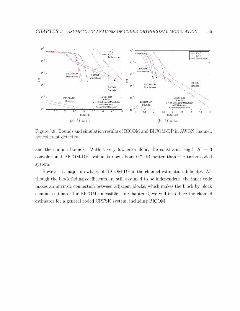
CHAPTER 3. ASYMPTOTIC ANALYSIS OF CODED ORTHOGONAL MODULATION 56
1 1.5 2 2.5 3 3.5 4 4.5 510
-10
10-8
10-6
10-4
10-2
100
Eb/No (dB)
BE
R
K = 3
K = 4
Turbo code
BICOM
Bounds
BICOM
Simulations
BICOM-DP
Simulations
BICOM-DP
Bounds
Length 6138
Rate ½
M = 16 Orthogonal Modulation
AWGN channel
Noncoherent Detection
(a) M = 16
Eb/No (dB)
BE
R
BICOM
Bounds
BICOM
Simulations
BICOM-DP
Simulations
BICOM-DP
Bounds
Length 6138
Rate ½
M = 64 Orthogonal Modulation
AWGN channel
Noncoherent Detection
1 1.5 2 2.5 3 3.5 4 4.5 510
-10
10-8
10-6
10-4
10-2
100
K = 3
K = 4
Turbo code
(b) M = 64
Figure 3.8: Bounds and simulation results of BICOM and BICOM-DP in AWGN channel,noncoherent detection
and their union bounds. With a very low error floor, the constraint length K = 3
convolutional BICOM-DP system is now about 0.7 dB better than the turbo coded
system.
However, a major drawback of BICOM-DP is the channel estimation difficulty. Al-
though the block fading coefficients are still assumed to be independent, the inner code
makes an intrinsic connection between adjacent blocks, which makes the block by block
channel estimator for BICOM unfeasible. In Chapter 6, we will introduce the channel
estimator for a general coded CPFSK system, including BICOM.

Chapter 4
Coherent CPFSK
The previous chapters focused on coded orthogonal modulation. One major drawback of
orthogonal modulation is its high bandwidth, since it requires M dimensions to transmit
m = log2 M bits.
This chapter begins our discussion of nonorthogonal continuous phase FSK (CPFSK)
modulation. In contrast with the orthogonal case, adjacent frequency tones can be placed
h/TS apart, where the modulation index h is usually between 0 and 1. Also, in CPFSK
modulation, the phase is continuous from symbol to symbol, which reduces the band-
width. The bandwidth efficiency can be further improved by using partial response
signaling, achieved by shaping the pulses prior to FM modulation. However, such a
strategy induces severe inter-symbol interference (ISI) which cannot be mitigated by a
truly noncoherent receiver. While the ISI can be resolved using differential detection,
such techniques are outside the scope of this dissertation. The interested reader is re-
ferred to [59] [60].
Unlike memoryless FSK, the phase of CPFSK is accumulated from symbol to symbol
to maintain a smooth phase transition. When the modulation index h is a rational
number, the accumulated phases take values from a finite set Φ ⊂ [0, 2π). In such a
case, the phase trajectory can be viewed as a finite-state Markov random process, so
that the modulator and additive white Gaussian noise (AWGN) channel can together be
considered as a finite-state Markov channel (FSMC). This allows coherent detection to
be performed on a trellis.
57

CHAPTER 4. COHERENT CPFSK 58
Finding the capacity of a FSMC is difficult, since it requires a maximization over
the probability density function (pdf) of a long input sequence. [61] studied the analyt-
ical bounds of discrete-time intersymbol interference (ISI) channel, one type of FSMC.
However, fortunately in practice, the input to the FSMC is usually preceded by an outer
channel encoder, which typically produces uniformly distributed outputs. Arnold et
al. [62] and Pfister et al. [63] use the forward recursion of the BCJR algorithm [9] to
compute the symmetric information rate of the FSMC, which is the mutual information
when the inputs are independent and uniformly distributed (i.u.d.). In this chapter, we
apply a similar approach to compute the symmetric information rate of coherently de-
tected CPFSK, which is to our knowledge a new application of the techniques in [62,63].
For the remainder of the chapter, we assume i.u.d. inputs and therefore use the term
capacity to specifically mean the symmetric information rate.
In this chapter, the signal model for coherent CPFSK in AWGN is introduced in
Section 4.1. Next, in Section 4.2 the i.u.d. capacity of coherent detected CPFSK is
evaluated by treating CPFSK and AWGN as a FSMC. Then, Section 4.3 analyzes the
capacity under spectral efficiency constraint.
Having established the capacity of coherent CPFSK, we turn our attention to the
design of systems that are capable of approaching the capacity. Iterative demodulation
and channel decoding of coded CPM systems was studied in [45,64], using convolutional
codes as outer codes. [65] considered a low density parity-check (LDPC) coded system
for minimum shift keying (MSK), achieving lower convergence threshold. In Section 4.4,
a binary irregular repeat-accumulate (IRA) code [66] is used along with iterative demod-
ulation and decoding with the CPFSK modulator assuming the role of the accumulator.
The IRA code is designed directly from the system’s EXIT chart using a curve-matching
technique proposed by ten Brink et al. [67] and Roumy et al. [68]. This method is adopted
in Section 4.5, and the optimization tool is linear programming, which was used by Chung
et al. [69] and Ardakani et al. [70] to find capacity approaching LDPC codes. This was
also applied to the noncoherent detection of orthogonal FSK by Guillen i Fabregas in [71],
where the area between inner and outer EXIT curves is minimized in order to find capac-
ity approaching code designs. The combination of IRA codes and CPM has previously
been considered in [72,73]. However, we point out later that the lower bound constraint

CHAPTER 4. COHERENT CPFSK 59
on degree one check node can be loosened, which potentially allows the optimized codes
to approach the capacity more closely. Simulation results in Section 4.6 show that our
coded system designs are only 0.4dB away from the coherent capacities of various M , h.
4.1 Coherent Detection
Suppose the input sequence to a CPFSK modulator is q, whose elements are i.u.d. over
the integers from 0 to M − 1. For every entry of q, the modulated signal xi(t) is chosen
as the qthi signal of the set S = {sk(t), k = 0, 1, · · · , M − 1}, where
sk(t) =1√Ts
exp
{j2πkht
Ts
}, t ∈ [0, Ts), (4.1)
and h is the modulation index. In order to satisfy the continuous-phase constraint, the
phase of each modulated symbol is accumulated as
φi+1 , φi + 2qihπ, (4.2)
where φi is the accumulated phase at the start of the ith symbol [59]. The complex-
baseband representation of the transmitted continuous-time waveform is√Ese
jφixi(t),
and the corresponding complex-baseband received signal is
yi(t) =√Ese
jφixi(t) + ni(t), (4.3)
where ni(t) is a circularly symmetric complex AWGN process with noise spectral density
N0, and Es is the energy per symbol [33].
Given the initial phase φi at the start of the ith interval, the front-end of the coherent
receiver determines the likelihoods of receiving yi(t) conditioned on each signal in S.
Since this process is the same for every received symbol, we drop the index i for the
remainder of this section. The received signal y(t), 0 ≤ t ≤ Ts, is first passed through a
bank of M pairs of matched filters, with one pair matched to the in-phase and quadrature
components of each tone, and then sampled at the symbol epoch. The sampled signal

CHAPTER 4. COHERENT CPFSK 60
can be written in vector form as
y = ejφ√Esx + n, (4.4)
where the elements of x and n are
xk =
∫ Ts
0
x(t)s∗k(t)dt (4.5)
nk =
∫ Ts
0
n(t)s∗k(t)dt, (4.6)
and k = {0, 1, ..., M − 1}. The noise vector n is Gaussian with a covariance matrix
R = E(nnH) with (k, i)th element
rk,i = N0
∫ Ts
0
s∗k(t)si(t)dt
= N0sin(π(i− k)h)
π(i− k)hejπ(i−k)h. (4.7)
When conditioned on both x and φ, the vector y is Gaussian with mean x and covariance
R, and has conditional pdf
p(y|x, φ) =1
πMdet(R)e−(y−ejφ
√Esx)HR−1(y−ejφ√Esx). (4.8)
The exponent can be simplified as
−(y − ejφ√Esx)HR−1(y − ejφ
√Esx)
= −yHR−1y − EsxHR−1x + 2Re(e−jφ
√Esx
HR−1y). (4.9)
Define K , 1N0
R, i.e. a normalized version of R. Note that when x(t) = sν(t), x is the
νth column of K. Therefore, given x(t) = sν(t), the exponent becomes
−yHK−1y + Es
N0
+ 2
√Es
N0
Re(e−jφyν). (4.10)
CHAPTER 4. COHERENT CPFSK 61
Taking the log of (4.8) and discarding terms that are common to all hypothesis, the log-
likelihood for coherent reception can be expressed for each postulated ν = {0, ..., M − 1}as
log f(y|x = kν , φ) = 2
√Es
N0
Re(e−jφyν), (4.11)
where kν represents the νth column of K and f(y|x, φ) ∝ p(y|x, φ).
4.2 Capacity of Coherent Detection
Trellis-based detection of CPFSK requires that the modulation index h be a rational
number so that the accumulated phase φ takes on values from a finite set. Suppose
h = P/Q, where P and Q are relatively prime positive integers. The total number of
unambiguous values that φ can assume is Q. Thus, demodulation can be performed over
a trellis with Q states and QM branches per trellis section.
In the following, the notation xji represents the set {xi,xi+1, · · · ,xj}. The capacity of
coherently detected CPFSK is found by first evaluating the average mutual information
I(xN−10 ,yN−1
0 ) between xN−10 and yN−1
0 , and then taking the average as the sequence
length N goes to infinity,
C(c) = limN→∞
1
NI(xN−1
0 ,yN−10 ). (4.12)
From the chain rule of entropy,
I(xN−10 ,yN−1
0 ) = H(xN−10 )−H(xN−1
0 |yN−10 )
=N−1∑i=0
H(xi)−N−1∑i=0
H(xi|xi−10 ,yN−1
0 ), (4.13)
where H(xi|xi−10 ) = H(xi) is used. Because xi is i.u.d. over M constellation points,
H(xi) = log2 M , and all that remains to be calculated is H(xi|xi−10 ,yN−1
0 ) . Note
that this factorization is different from the factorization I(xN−10 ,yN−1
0 ) = H(yN−10 ) −
H(yN−10 |xN−1
0 ) used in [62,63], which requires the calculation of two entropies. From the

CHAPTER 4. COHERENT CPFSK 62
definition of conditional entropy,
H(xi|xi−10 ,yN−1
0 ) = −E[log2 p(xi|xi−1
0 ,yN−10 )
]. (4.14)
The above expectation can be found using Monte Carlo integration.
To compute the probability p(xi|xi−10 ,yN−1
0 ), first apply Bayes’ rule to obtain
p(xi|xi−10 ,yN−1
0 ) =p(xi,x
i−10 ,yN−1
0 )
p(xi−10 ,yN−1
0 ). (4.15)
Rather than explicitly calculating the denominator in (4.15), its value is found to ensure
that
∑xi
p(xi|xi−10 ,yN−1
0 ) = 1. (4.16)
Similar to [62], a BCJR-like method can be used to compute p(xi,xi−10 ,yN−1
0 ), which is
described as follows. Assume φ takes on values from the set Φ, whose cardinality is Q.
Define α, β, γ as
αi(φi) , p(φi,yi−10 ,xi−1
0 ) (4.17)
βi+1(φi+1) , p(yN−1i+1 |φi+1) (4.18)
γ(φi → φi+1,yi,xi) , p(yi, φi+1|φi,xi). (4.19)
Note that γ(φi → φi+1,yi,xi) is nonzero only when xi causes the state transition from
φi to φi+1. Therefore, it may be written as
γ(φi → φi+1,yi,xi = kν)
= p(φi+1|φi,xi = kν)p(yi|φi+1, φi,xi = kν)
=
{p(yi|φi,xi = kν) φi+1 = φi + 2νhπ
0 φi+1 6= φi + 2νhπ.(4.20)

CHAPTER 4. COHERENT CPFSK 63
As with the BCJR algorithm, α can be calculated in a forward recursion as
αi+1(φi+1) =1
M
∑
φi∈Φ
αi(φi)γ(φi → φi+1,yi,xi = kqi). (4.21)
Similarly, β can be calculated in a backward recursion as
βi(φi) =1
M
∑xi
∑
φi+1∈Φ
βi+1(φi+1)γ(φi → φi+1,yi,xi). (4.22)
Note that xi is marginalized out of the summand since βi(φi) does not depend on it.
In the absence of knowing the starting and ending states, both α0 and βN can be
initialized assuming equally likely states, i.e. α0(φ) = βN(φ) = 1/M , ∀φ ∈ Φ. Alterna-
tively, if the initial phase φ0 is known to the detector, α0 can be set to all zeros except
a one at the corresponding entry. Obviously, the effect of the initial states of α0 and βN
diminish as N approaches infinity.
Given the above definitions, p(xi,xi−10 ,yN−1
0 ) is found from
p(xi,xi−10 ,yN−1
0 ) =1
M
∑
φi∈Φ
∑
φi+1∈Φ
αi(φi)βi+1(φi+1)γ(φi → φi+1,yi,xi). (4.23)
Fig. 4.1 shows the capacities of different detectors of MSK (M = 2, h = 1/2). From
left to right, they are i.u.d. capacity of coherent detection, i.u.d. capacity of BICM de-
tection [21] and symbol-wise noncoherent capacity [22] respectively. The BICM detector
uses the coherent metric in (4.11) and decodes through the trellis as well. However, it as-
sumes no priori information, and measures the mutual information at the decoder output.
Therefore, the BICM capacity of MSK is strictly bounded by the coherent capacity.
C(BICM) = limN→∞
1
N
N−1∑i=0
[H(xi)−H(xi|yN−1
0 )]. (4.24)
< limN→∞
1
N
N−1∑i=0
[H(xi)−H(xi|xi−1
0 yN−10 )
].
= C(c)

CHAPTER 4. COHERENT CPFSK 64
-30 -25 -20 -15 -10 -5 0 5 10 15 200
0.2
0.4
0.6
0.8
1
1.2
Es/No
Capa
city
Coherent i.u.d. CapacityBICMnoncoherent capacity
Figure 4.1: Capacities of MSK (M = 2, h = 1/2): From left to right, they are i.u.d.capacity of coherent detection, i.u.d. capacity of BICM detection and symbol-wise non-coherent capacity respectively.
At coding rate r = 0.5, the gap between BICM capacity and coherent capacity is about
2.5dB. This also tells that the iterative decoding of coherent CPFSK is desirable, because
the extrinsic information can help the CPFSK detector exploits more information from
the trellis.
4.3 Capacity under Spectral Efficiency Constraint
For coherent detection, it is generally true that the minimum Eb/N0 required is a mono-
tonic increasing function over the coding rate r. But lower coding rates require wider
bandwidth, which reduces the spectral efficiency. To quantify the tradeoff between Eb/N0
and spectral efficiency, the bandwidth of the CPFSK signal must be computed. The
power spectral density (PSD) Ψs(f) of the CPFSK signal s(t) is given in Section 4.4.2

CHAPTER 4. COHERENT CPFSK 65
of [32]. From the PSD, the 99% power bandwidth B99 of s(t) is defined as
∫ B99/2
−B99/2
Ψs(f)df = 0.99
∫ ∞
−∞Ψs(f)df. (4.25)
This bandwidth is a function of M , h, and the symbol rate Rs = 1/Ts. Given that
s(t) with parameters M and h is transmitted at a rate of Rs baud, we can define the
normalized bandwidth to be B(M, h) = B99Ts Hz/baud. We can then define the spectral
efficiency η = r log2 M/B(M, h), which has units of bits-per-second-per-Hz (bps/Hz).
To determine the fundamental tradeoff between η and Eb/N0, one must determine the
minimum value of Eb/N0 for a particular desired spectral efficiency η. For each choice
of η, h, and M , the range of r that may be considered is restricted, and there will be a
threshold r′ on code rate
r′ = ηB(M, h)
log2 M(4.26)
such that r ∈ [r′, 1]. Rates r < r′ cannot be considered because for the particular h
and M , the spectral efficiency will be lower than η. For coherent detection, given the
fact that Eb/N0 monotonically increases with respect to the coding rate r, r′ is the point
where the minimum Eb/N0 can be achieved. Note that this is different from the case of
noncoherent detection, where the optimal coding rate could be anywhere in the range
[r′, 1] due to the noncoherent combining penalty [17,22].
Determining of the minimum Eb/N0 for each choice of M , h, and η requires that the
curve showing Eb/N0 versus r be generated. Next, the minimum rate r′ is determined. For
example, when M = 2 and η = 1/2 bps/Hz, the minimum values of r are 0.39, 0.55, 0.64,
and 0.96 for h = 1F/5, 2/5, 3/5, and 4/5, respectively. Since B(M = 2, h = 1) =
2.1309 > 1/η, no code of rate r ≤ 1 can be used at this η when h = 1 and thus
orthogonal modulation cannot be considered. Next, the minimum Eb/N0 at coding rate
r′ is found.
Fig. 4.2 shows the binary CPFSK capacity for different spectral efficiencies. To
constrain complexity, we restrict the denominator of h to assume values Q ≤ 5. For the
loosest constraint (η = 0.02), the minimum Eb/N0 required approaches −1.6 dB for every

CHAPTER 4. COHERENT CPFSK 66
0.1 0.2 0.3 0.4 0.5 0.6 0.7 0.8 0.9 1-2
-1
0
1
2
3
4
5
h
min
Eb/
No
= 0.75
= 0.25
= 0.02
= 0.5
Figure 4.2: Capacities of binary CPFSK for different spectral efficiency constraints. Fromtop to bottom, the spectral efficiencies are η = 0.75, η = 0.5, η = 0.25 and η = 0.02. his considered with the denominator up to 5. So from left to right, they are 1
5, 1
4, 1
3, 2
5,
12, 3
5, 2
3, 3
4and 4
5respectively. Also, the memoryless orthogonal case h = 1 is listed for
reference.
choice of h. As the bandwidth gets tighter, the required Eb/N0 becomes larger. When
η = 0.25, the minimum Eb/N0 is about −1 dB, and it is achieved at h = 35
and coding
rate r = 0.32. When η = 0.5, the minimum Eb/N0 = −0.1 dB is still achieved at h = 35,
and the coding rate is doubled to about 0.64. When η = 0.75, the minimum Eb/N0 = 1.9
dB is achieved at h = 25, and the optimal coding rate is r = 0.83.
Fig. 4.3 shows the CPFSK capacities of different M under spectral efficiency η = 0.5.
The optimal choice of h and r for each M is listed in Table 4.1.
4.4 Coded System Implementation
The structure of a coded system capable of approaching the CPFSK capacity limits is
shown in Fig. 4.4. The system is a serial concatenation of two codes separated by an

CHAPTER 4. COHERENT CPFSK 67
0.1 0.2 0.3 0.4 0.5 0.6 0.7 0.8 0.9-1
-0.5
0
0.5
1
1.5
2
2.5
3
h
min
Eb/
No
M=2M=4M=8
Figure 4.3: CPFSK capacities of different M for spectral efficiency η = 0.5. h is consid-ered with the denominator up to 5. So from left to right, they are 1
5, 1
4, 1
3, 2
5, 1
2, 3
5, 2
3, 3
4
and 45
respectively.
interleaver Π. The outer code is a mixture of repetition codes represented by variable
nodes “=”. The degree d of a variable node is the number of times that the corresponding
message bit is repeated. Since the code is irregular, the variable nodes do not all have the
same degree. The entire set of repeated bits is interleaved and sent to the check nodes,
represented by “+”. Each check node forms a single party-check (SPC) on a distinct
subset of interleaved bits. The degree of a check node is the number of bits used to
form the check. The outputs of the SPC nodes are grouped together and passed to the
modulator. As in [74], the code is nonsystematic, and therefore unlike [68], the message
bits are not modulated.
The system shown in Fig. 4.4 is reminiscent of the IRA code proposed in [66]. When
used with a memoryless modulation, an IRA code must include an accumulator to ensure
that the inner code is recursive. However, as evident by (4.2), CPFSK with noninteger
h is already recursive. Thus, as observed in [72], a coherent nonorthogonal CPM system
does not need an accumulator because the recursive modulator may assume the role of

CHAPTER 4. COHERENT CPFSK 68
+=
= + Parallel/S
erial
CPFSK
zi
vi
ri,j
mi,jFigure 4.4: Nonsystematic IRA coding structure. “=” corresponds to variable nodes and“+” corresponds to single parity-check nodes.
the accumulator.
At the transmitter, a binary message vector u ∈ {0, 1}Nu is encoded in parallel by Nu
variable nodes, each generating a repetition code. In the factor-graph representation of
the code, the degree d of a node is the number of edges that are incident to the node. The
degree distribution of the variable nodes can be described by either the node-perspective
degree distribution λd or the edge-perspective degree distribution λd. In particular, λd is
the fraction of nodes that have degree d, while the λd is the fraction of edges that touch
degree d nodes. The two perspectives are related by
λi =λii∑dv
d=1 λdd(4.27)
where dv is the maximum variable-node degree.
The outputs from the Nu variable nodes form a vector c′ of length Nc =∑dv
d=1 λddNu.
c′ is then interleaved into c and forwarded to Nb single-parity-check nodes. The check-
node degree distributions may be represented in either node-perspective ρd or edge-
perspective ρd. The variables Nb and Nc are related by Nb = Nc/(∑dc
d=1 ρdd), where dc
is the maximum check-node degree. Each check node computes the single parity-check

CHAPTER 4. COHERENT CPFSK 69
bit of its inputs, and forms the vector b for modulation. Therefore, the coding rate r
satisfies
r =
∑dc
d=1 ρdd∑dv
d=1 λdd=
∑dv
d=1λd
d∑dc
d=1ρd
d
. (4.28)
Before it is modulated, the binary vector of bits b must be transformed into the M-ary
symbol vector q by an appropriate symbol labeling function g(·), which can be expressed
as
qi = g
(µ−1∑j=0
biµ+j2µ−1−j
), (4.29)
where µ = log2 M . In this chapter, we simply assume Nb is divisible by µ. Otherwise,
b can be padded to meet this requirement. Therefore, q is a M-ary vector of length
N = Nb/µ. For the binary case, labeling is not important, since the two frequency
tones are interchangeable. However, when M is greater than 2, the labeling can be very
important for certain values of h. This point will be discussed in the next section.
At the receiver, decoders for each of the inner and outer codes exchange extrinsic
information using a turbo-like schedule [68], or equivalently using the sum-product al-
gorithm [75]. Fig. 4.4 also shows the extrinsic information flow using dashed arrows.
During the first stage, based on the channel observation yN−10 , the log likelihood ratios
z are found by using the BCJR [9] or SISO [35] decoding algorithm. The jth element of
z is
zj = logp(bj = 0|yN−1
0 ,v\vj)
p(bj = 1|yN−10 ,v\vj)
, (4.30)
where v is the extrinsic information from the check nodes, and \vj indicates that vj
is excluded, so that zj carries extrinsic information only. Obviously, in the first half
decoding iteration, v is all zeros.
The check nodes then update the messages sent to the variable nodes. The output
information ri,j from jth check node to ith variable node, assuming they are connected,
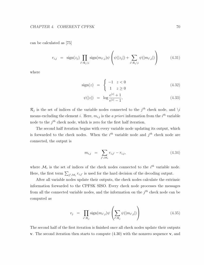
CHAPTER 4. COHERENT CPFSK 70
can be calculated as [75]
ri,j = sign(zj)∏
i′:Rj\isign(mi′,j)ψ
ψ(|zj|) +
∑
i′:Rj\iψ(|mi′,j|)
(4.31)
where
sign(z) =
{−1 z < 0
1 z ≥ 0(4.32)
ψ(|z|) = loge|z| + 1
e|z| − 1, (4.33)
Rj is the set of indices of the variable nodes connected to the jth check node, and \imeans excluding the element i. Here, mi,j is the a priori information from the ith variable
node to the jth check node, which is zero for the first half iteration.
The second half iteration begins with every variable node updating its output, which
is forwarded to the check nodes. When the ith variable node and jth check node are
connected, the output is
mi,j =∑
j′:Mi
ri,j′ − ri,j, (4.34)
where Mi is the set of indices of the check nodes connected to the ith variable node.
Here, the first term∑
j′:Miri,j′ is used for the hard decision of the decoding output.
After all variable nodes update their outputs, the check nodes calculate the extrinsic
information forwarded to the CPFSK SISO. Every check node processes the messages
from all the connected variable nodes, and the information on the jth check node can be
computed as
vj =∏
i′:Rj
sign(mi′,j)ψ
∑
i′:Rj
ψ(|mi′,j|) (4.35)
The second half of the first iteration is finished once all check nodes update their outputs
v. The second iteration then starts to compute (4.30) with the nonzero sequence v, and

CHAPTER 4. COHERENT CPFSK 71
performs (4.31), (4.34) and (4.35) accordingly. It is feasible that the variable nodes and
check nodes can perform several local iterations within a single global iteration. That
is, (4.31) and (4.34) are evaluated more than once before (4.30) is executed in the next
global iteration. But in this chapter, in order to exploit the most information from the
CPFSK trellis, we only perform (4.31) and (4.34) once per global iteration.
4.5 Code Optimization
EXIT charts are often used to analyze the convergence behavior of iterative decoding
systems. In [67], a curve-matching technique was applied that allows EXIT charts to
be directly used as a code design methodology. This technique was later applied to the
design of IRA codes in [68] and systems using orthogonal FSK with symbol-by-symbol
noncoherent detection in [74]. Here, we apply the EXIT curve-matching technique to
design nonsystematic IRA codes for CPFSK with coherent detection.
An EXIT chart is created for a particular SNR by drawing the information-transfer
functions for the inner and outer codes on the same plot. The information-transfer
function for an outer repetition code of degree d is [76]
I(o)E,d(I
(o)A ) = J
(√d− 1J−1(I
(o)A )
), (4.36)
where the superscript (o) denotes the outer code, and the subscripts A and E represent
the a priori input information and the extrinsic output information. The function J(·)is defined in [76] as
J(σ) =
∫1
2πσe−
(x−σ2)2
2σ2 log2
(1 + e−x
)dx, (4.37)
and can be predetermined by numerical or Monte Carlo integration.
When an IRA code is used, the variable nodes do not all have the same degree. The
overall information-transfer function for the outer code can be approximated by using
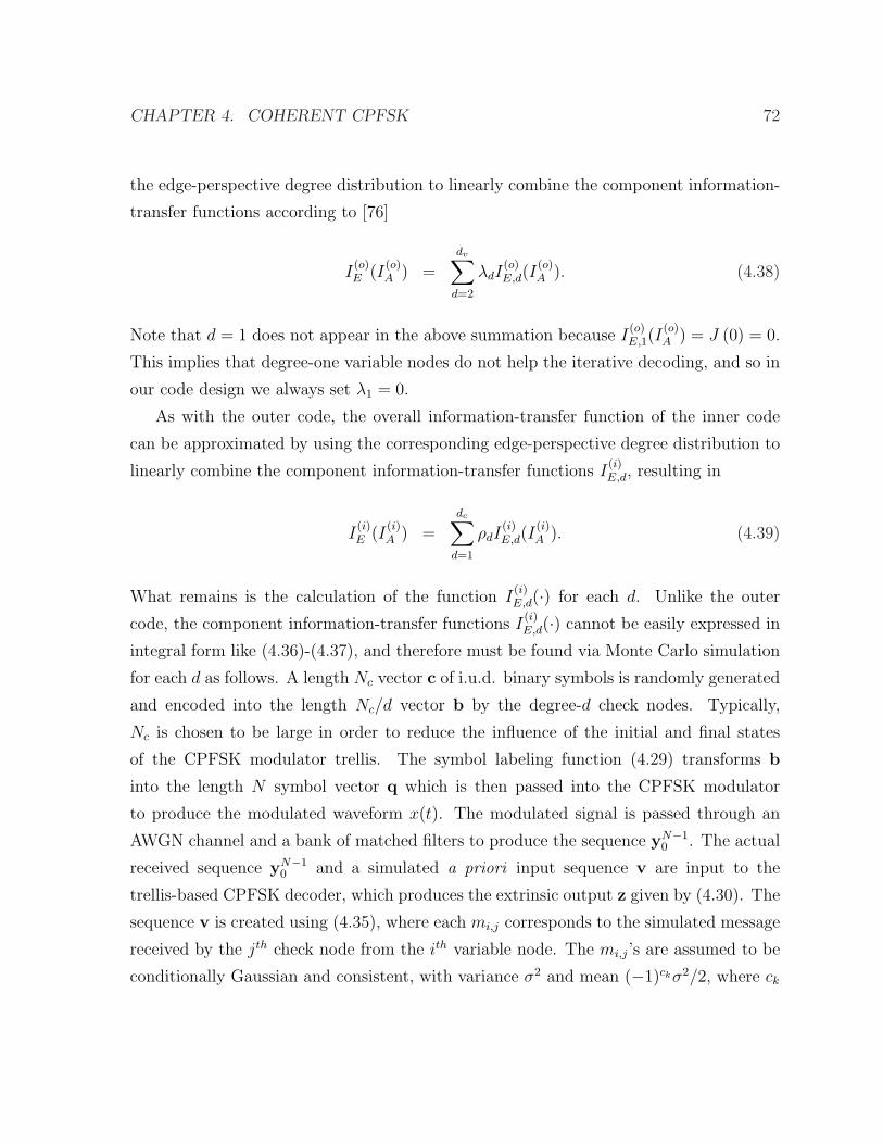
CHAPTER 4. COHERENT CPFSK 72
the edge-perspective degree distribution to linearly combine the component information-
transfer functions according to [76]
I(o)E (I
(o)A ) =
dv∑
d=2
λdI(o)E,d(I
(o)A ). (4.38)
Note that d = 1 does not appear in the above summation because I(o)E,1(I
(o)A ) = J (0) = 0.
This implies that degree-one variable nodes do not help the iterative decoding, and so in
our code design we always set λ1 = 0.
As with the outer code, the overall information-transfer function of the inner code
can be approximated by using the corresponding edge-perspective degree distribution to
linearly combine the component information-transfer functions I(i)E,d, resulting in
I(i)E (I
(i)A ) =
dc∑
d=1
ρdI(i)E,d(I
(i)A ). (4.39)
What remains is the calculation of the function I(i)E,d(·) for each d. Unlike the outer
code, the component information-transfer functions I(i)E,d(·) cannot be easily expressed in
integral form like (4.36)-(4.37), and therefore must be found via Monte Carlo simulation
for each d as follows. A length Nc vector c of i.u.d. binary symbols is randomly generated
and encoded into the length Nc/d vector b by the degree-d check nodes. Typically,
Nc is chosen to be large in order to reduce the influence of the initial and final states
of the CPFSK modulator trellis. The symbol labeling function (4.29) transforms b
into the length N symbol vector q which is then passed into the CPFSK modulator
to produce the modulated waveform x(t). The modulated signal is passed through an
AWGN channel and a bank of matched filters to produce the sequence yN−10 . The actual
received sequence yN−10 and a simulated a priori input sequence v are input to the
trellis-based CPFSK decoder, which produces the extrinsic output z given by (4.30). The
sequence v is created using (4.35), where each mi,j corresponds to the simulated message
received by the jth check node from the ith variable node. The mi,j’s are assumed to be
conditionally Gaussian and consistent, with variance σ2 and mean (−1)ckσ2/2, where ck

CHAPTER 4. COHERENT CPFSK 73
is the corresponding simulated bit of c. The variance σ2 is found from the information-
transfer function’s argument I(i)A by inverting (4.37). Once z is generated, (4.31) is
used to generate the messages ri,j sent from the check nodes to the variable nodes.
Finally, an estimate of I(i)E,d(·) is found for the given codeword and channel realization by
measuring the mutual information between c and the corresponding ri,j’s. The process is
repeated for many simulated codewords and channel realizations, and the sample mean
is computed.
Once the information-transfer functions for the inner and outer codes have been found,
they are drawn on the same plot. The inner-code’s information-transfer function is
drawn with I(i)A as its horizontal axis and I
(i)E as its vertical axis, while the outer-code’s
information-transfer function is drawn with I(o)E as its horizontal axis and I
(o)A as its
vertical axis. The plot showing both of these curves constitutes the system’s EXIT
chart. The code is said to converge if there is a gap between the two curves, and the
convergence threshold is the minimum SNR for which the two curves just barely touch.
The design objective is to minimize this threshold through the proper selection of the
degree distributions.
4.5.1 Degree Distribution Optimization
The convergence threshold can generally be minimized by minimizing the area between
the inner and outer EXIT curves. This property was used in [74] and [77] to design
capacity-approaching codes. We apply the same principle by first fixing the degree dis-
tribution of the inner code {ρd} and the channel SNR Es/N0, and then finding the degree
distribution of the outer code {λd} that minimizes the area between the curves. This can
be done by using linear programming. We sample the outer-code’s EXIT curve I(o)E (·)
along the I(o)A axis and the inner-code’s inverse EXIT curve I
(i)A (·) = I
(i)−1E (·) along the
I(o)E axis. Let Ii ∈ (0, 1) denote the ith sampling point and I denote the indices of the
sampling points. Convergence requires the two curves do not intersect, which implies
that I(i)A (Ii) < I
(o)E (Ii) for all i ∈ I. When there are a large number of uniformly spaced

CHAPTER 4. COHERENT CPFSK 74
sampling points, the area between the two curves can be approximated as
A ∝∑i∈I
(I
(o)E (Ii)− I
(i)A (Ii)
). (4.40)
Given that the maximum variable-node degree is dv, the area A in (4.40) can be minimized
subject to the following constraints: (1) I(i)A (Ii) < I
(o)E (Ii) for all i ∈ I; (2)
∑dv
d=2 λd = 1;
and (3) The desired coding rate r in (4.28) is attained. If a solution to the linear
programming problem is found for a particular channel SNR Es/No, then the SNR is
lowered and the process repeated until a solution can no longer be found. The final
design and the convergence threshold is found from the last successful solution to the
linear programming problem.
4.5.2 Symbol Labeling Issues
When M is greater than Q, the denominator of h, the number of edges coming out of
each state is more than the total number of states. When this occurs, there will be
parallel edges between at least one pair of starting and stopping states. This is apparent
by inspecting (4.2). For example, when M = 4 and h = 1/3 and the starting state is φi,
the symbol-wise inputs q = 0 and q = 3 share the same ending state φi+1 = φi = φi +2π.
As shown in Fig. 4.6, the symbols may be labeled according to either a Gray labeling or
a natural labeling.
The symbol labeling function has a profound effect on the shape of the inner-code’s
EXIT curve. Fig. 4.5 shows the EXIT curves for M = 4 h = 1/3 at Es/N0 = 0 dB with
Gray and natural labelings. The effect of the symbol labeling is most pronounced on the
right side of the EXIT curves. With natural labeling, the EXIT curves for codes with
degree one and two terminate in the upper right corner, i.e. the (1, 1) point. However,
with Gray labeling, when the input a priori information is perfect, the output extrinsic
information is only about 7/8. This means that even when all other bits are perfectly
known, there is still some uncertainty about the current bit. The underlying reason is
the labeling. With Gray labeling, there exist parallel transitions labeled with 00 and
10. In this case, when all the other bits are known, and the starting and ending states

CHAPTER 4. COHERENT CPFSK 75
IA(i)
I E(i)
0 0.1 0.2 0.3 0.4 0.5 0.6 0.7 0.8 0.9 10
0.1
0.2
0.3
0.4
0.5
0.6
0.7
0.8
0.9
1Natural labelingGray labeling
d=1
d=2
Figure 4.5: Inner code EXIT curves of M = 4, h = 1/3 with gray and natural labelings.Es/N0 = 0dB.
can be perfectly identified, the first bit still can not be identified for sure. For instance,
if the decoder knows that the starting and ending states are zero and that the second
bit associated with the state transition is zero, then the decoder cannot determine if the
first bit is a zero or a one. However, with natural labeling, the parallel transitions are
labeled with 00 and 11, which means either bit can be determined provided the other
one is perfectly known.
When the inner-code’s EXIT curve does not terminate in the upper right, the code
optimization technique described in the previous section will not work because I(i)A (Ii) <
I(o)E (Ii) will not be satisfied as Ii approaches unity. In addition to violating the linear
programming constraint, the code will have a high error floor due to the early crossing of
the inner-code and outer-code EXIT curves. To prevent these issues, the symbol labeling
should be chosen to assure that the inner-code EXIT curve extends to the (1, 1) point.
Thus, for the example of M = 4 and h = 1/3, natural labeling is more desirable than
Gray labeling. However, natural labeling is not universally preferred. For instance when

CHAPTER 4. COHERENT CPFSK 76
000011011 0
Gray Labeling
000011110 0
Natural LabelingFigure 4.6: Gray and natural labelings of M = 4, h = 1/3
M = 8 h = 1/4, Gray labeling is preferred over natural labeling. As a general rule, a
suitable labeling is one that assures that parallel transition pairs are labeled with at least
two distinct bits. This rule is the sufficient and necessary to force the inner-code EXIT
curve to the (1, 1) point.
4.5.3 Interleaver Design Issues
If an interleaver is drawn at random, there is a possibility that the resulting encoder will
perform a many-to-one mapping of message sequences u to codewords b. Two examples
of when this situation occurs are shown in Fig. 4.7. In the example on the left, a
particular variable node is connected to a check node by an even number d of parallel
edges. In such a case, the check node will take the modulo-2 sum of the bit at the output
of the variable node, which is always equal to zero no matter what bit is produced by
the variable node. It is as if the two nodes were not connected. If the variable node is
not connected to any other check node by an odd number of edges, then the receiver
will not be able to determine the likelihood associated with the variable node no matter
how high the SNR. For a variable node of degree d = 2, the probability of this situation

CHAPTER 4. COHERENT CPFSK 77
+=
=+
+=
Figure 4.7: Bad interleaver designs
occurring in a purely random intelerleaver is bounded by
Pbad ≤(
Nuλ2
1
) ∑dc
d=2
(Nbρd
1
)(d2
)2!(Nc − 2)!
Nc!. (4.41)
When the degree distributions are fixed, Nu and Nb are proportional to Nc. It is not hard
to see that the bound reaches some constant value when the interleaver size Nc keeps
increasing.
Another example is shown in the right side of Fig. 4.7, where two variable nodes of
degree two are linked to two check nodes of degree two in a butterfly structure. When
this occurs, the two check nodes will produce the same output value. While this output
may be used to determine the modulo-2 sum of the bits associated with the two variable
nodes, it will not reveal their individual values. The probability of this situation can be
bounded by
Pbad ≤ 16(
Nuλ2
2
)(Nbρ2
2
)(Nc − 4)!
Nc!
≈ 4(Nuλ2)2(Nbρ2)
2
N4c
. (4.42)
This approximation is a constant that does not depend on the interleaver size. However,
this constant behavior only exists for degree-two variable nodes. It is not hard to verify
that the probability of bad interleaver designs caused by variable nodes with degree
three and above decreases when the interleaver size Nc increases. This implies that
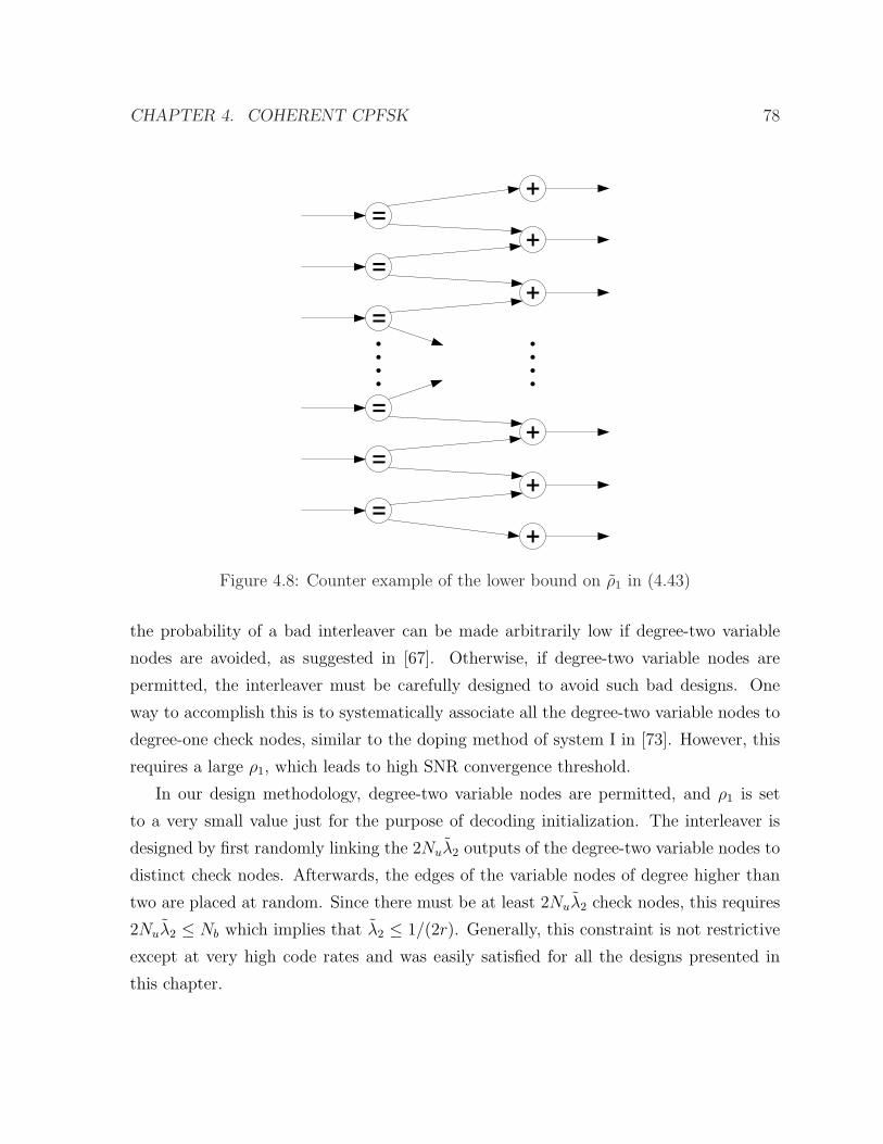
CHAPTER 4. COHERENT CPFSK 78
+=
=+
+=
+=
=
+
+=
Figure 4.8: Counter example of the lower bound on ρ1 in (4.43)
the probability of a bad interleaver can be made arbitrarily low if degree-two variable
nodes are avoided, as suggested in [67]. Otherwise, if degree-two variable nodes are
permitted, the interleaver must be carefully designed to avoid such bad designs. One
way to accomplish this is to systematically associate all the degree-two variable nodes to
degree-one check nodes, similar to the doping method of system I in [73]. However, this
requires a large ρ1, which leads to high SNR convergence threshold.
In our design methodology, degree-two variable nodes are permitted, and ρ1 is set
to a very small value just for the purpose of decoding initialization. The interleaver is
designed by first randomly linking the 2Nuλ2 outputs of the degree-two variable nodes to
distinct check nodes. Afterwards, the edges of the variable nodes of degree higher than
two are placed at random. Since there must be at least 2Nuλ2 check nodes, this requires
2Nuλ2 ≤ Nb which implies that λ2 ≤ 1/(2r). Generally, this constraint is not restrictive
except at very high code rates and was easily satisfied for all the designs presented in
this chapter.

CHAPTER 4. COHERENT CPFSK 79
A guideline given in [72] is that when the check nodes have degrees of either one or
dc, then the doping rate ρ1 should satisfy
ρ1 ≥ dc − 1
dv + dc − 1. (4.43)
This bound is suitable if only one iteration is performed. However, if multiple iterations
are permitted, ρ1 does not have to satisfy this criteria. This is illustrated by the inter-
leaver shown in Fig. 4.8 which serves as a counter-example. In the counter-example, all
variable nodes have degree two and the check nodes may have degree one or two. The
bound (4.43) would imply that at least 1/3 of the check nodes should have degree one
in order to permit successful decoding. However, in Fig. 4.8, there are only two check
nodes of degree one, and therefore ρ1 could be quite small. During each iteration of de-
coding, the information from the degree-one nodes at the top and bottom will propagate
towards the center of the graph. Thus, the system is decodable given a sufficient number
of iterations, despite not adhering to to (4.43).
This also implies that with a large maximum number of iterations allowed, ρ1 could
be made to a very small number. In this chapter, our code designs are all based on the
check nodes with degree distribution ρ1 = 0.001 and ρ2 = 0.999, because a fairly early
waterfall can be achieved using this distribution, while the decoding is still manageable
in 200 iterations.
4.6 Optimization and Simulation Results
Code optimizations were performed for the systems that achieved the information-theoretic
minimum Eb/N0 at spectral efficiency η = 0.5 bps/Hz. Three alphabet sizes were con-
sidered, M = {2, 4, 8}. As optimal choice of h and r for each M is shown in Table 4.1.
In addition, we also considered a suboptimal choice for M = 2 (with h = 2/5) and a
suboptimal choice for M = 4 (with h = 1/3). In each case, the inner-code’s degree dis-
tribution was set to ρ1 = 0.001 and ρ2 = 0.999. A very small number of degree-one check
nodes are needed to allow the iterative decoding process to start properly. Otherwise,
the decoding process always stays at the origin of the EXIT chart [72]. Setting a smaller

CHAPTER 4. COHERENT CPFSK 80
I E(i) ,I A(o)
IA(i),IE(o)Repetition codes
Combined parity-check codes and CPFSK
Eb/N0 = -0.01 dBr = 0.4865M=4, h=1/3
Natural Labeling
0 0.2 0.4 0.6 0.8 10
0.2
0.4
0.6
0.8
1
Figure 4.9: Optimized EXIT curves for M = 4, h = 1/3 with natural labeling.
ρ1 could help the decoder converge in fewer iterations, but the required Eb/N0 tends to
be higher.
Having fixed the inner-code’s degree distribution, the outer-code’s degree distribution
was found using linear programming under the constraint that the maximum outer-code
degree is dv = 20. Gray labeling was used for the M = 8 system, and natural labeling
for the M = 4 system. EXIT curves for the optimized system with parameters M = 4
h = 1/3 and r = 0.4865 are shown in Fig. 4.9. From the EXIT curves, the convergence
threshold is found to be Eb/N0 = −0.01 dB, and the optimized variable node degree
distribution is λ2 = 0.0714, λ3 = 0.4926 and λ10 = 0.3417. The optimized degree
distributions and convergence thresholds are shown for all five systems in Table 4.1. The
table also lists the Eb/N0 required for an actual system to achieve a simulated bit error
probability of 10−5. For each system, Nu = 100, 000 message bits are used and 200
decoding iterations are performed. For all five systems, the simulation results are about
0.4 dB from the capacity limit.
Fig. 4.10 shows the BER curve of the optimized M = 4, h = 1/3 and r = 0.4865

CHAPTER 4. COHERENT CPFSK 81
Capacity
-0.2 -0.1 0 0.1 0.2 0.3
10-410-310-210-1100
Eb /N0
BER
10-5Figure 4.10: BER of optimized M = 4, h = 1/3 system. The system has uncodedbits Nu = 100, 000, and the figure shows the BERs of 50,60,70,80,90,100,150 and 200iterations from top to bottom.
system in Table 4.1. For this system, the number of degree-one and degree-two check
nodes are 411 and 205135, respectively, while the number of degree-two, degree-three,
and degree-ten variable nodes are 14661, 67433, and 17906 respectively. For coherent
detection, the Eb/N0 required to achieve a BER of 10−5 is 0.23 dB, about 0.24 dB from
the estimated threshold and 0.37 dB from the capacity limit.
4.7 Chapter Summary
Before engaging in the design of capacity-approaching codes for CPFSK modulation,
it is useful to compute the AWGN modulation-constrained capacity limits for a given
alphabet size M and modulation index h. This computation is facilitated by treating
CPFSK over AWGN channels as a finite-state Markov channel and then computing the
i.u.d. capacity using the proposed BCJR-like algorithm. In addition to serving as a

CHAPTER 4. COHERENT CPFSK 82
Table 4.1: Capacity and code optimization results for spectral efficiency η = 0.5 bps/Hz.The ith element of the labeling vector is the octal value of the bit pattern labeling symbolqi. The simulation Eb/N0 is the value for which a system with Nu = 100, 000 messagebits and 200 decoder iterations reaches a simulated BER of 10−5.
M 2 4 8h 2
535
13
25
14
r 0.5535 0.6428 0.4865 0.5410 0.4458Capacity(Eb/N0) 0.02dB −0.1dB −0.14dB −0.31dB −0.4dB
Labeling Natural Natural Natural Natural Gray[0,1] [0,1] [0,1,2,3] [0,1,2,3] [0,1,3,2,6,7,5,4]
λ2 = 0.1752 λ2 = 0.3 λ2 = 0.0714 λ2 = 0.2056 λ3 = 0.4947Variable node λ3 = 0.4315 λ3 = 0.3461 λ3 = 0.4926 λ3 = 0.3937 λ4 = 0.0577
distribution {λd} λ8 = 0.1369 λ6 = 0.2435 λ10 = 0.4360 λ9 = 0.0152 λ10 = 0.3417λ9 = 0.2564 λ7 = 0.1104 λ11 = 0.3855 λ11 = 0.1059
Check node ρ1 = 0.001 ρ1 = 0.001 ρ1 = 0.001 ρ1 = 0.001 ρ1 = 0.001distribution {ρd} ρ2 = 0.999 ρ2 = 0.999 ρ2 = 0.999 ρ2 = 0.999 ρ2 = 0.999Threshold(Eb/N0) 0.14dB 0.03dB −0.01dB −0.22dB −0.19dB
Simulation(Eb/N0) 0.35dB 0.31dB 0.23dB 0.06dB 0.01dB
benchmark to measure the effectiveness of actual coded systems, the capacity analysis
provides useful insight into the optimal selection of the parameters M and h. This is
especially important when bandwidth is constrained, in which case there will be a lower
limit on the allowable code rate r which depends on the choice of M and h. Usually,
complexity concerns requires that h = P/Q be rational with a small denominator Q.
Thus for any particular spectral efficiency, alphabet size M , and complexity limit, there
will be an optimal combination of r and h that can be found through capacity analysis.
Once the system parameters and corresponding modulation-constrained capacity are
determined, the next step in the system design is to optimize the code. This is done
with the aid of the EXIT chart. First the EXIT curve for the inner code is drawn for a
particular target-channel SNR, where the inner code is the combination of single-parity-
check codes and CPFSK modulation. The outer-code degree distribution is determined
through linear programming with the objective of minimizing the area between the inner-
code and outer-code EXIT curves. The optimal design is the one that minimizes this area
at the lowest channel SNR without allowing the two curves to cross. Results show that
this threshold SNR is between 0.1 and 0.2 dB from the value predicted by corresponding

CHAPTER 4. COHERENT CPFSK 83
capacity limit. Certain care must be taken to avoid bad interleavers and symbol labelings.
Simulation results using the actual coded system achieve a BER of 10−5 at only about
0.4 dB from the capacity with a message length of 105 and 200 decoder iterations. While
the system performed remarkably close to capacity, we made no particular attempt to
optimize the inner code. The whole process could be repeated for different inner code
designs, which could result in a design that is even closer to the corresponding capacity
limits.

Chapter 5
Noncoherent CPFSK
One of the benefits of using CPFSK is that it can be noncoherently detected. Despite
having a capacity that is lower than coherent detection, there are significant complexity
benefits to use noncoherent detection. As discussed in the previous chapter, for coherent
detection to be feasible, h must be a rational number, i.e. h = P/Q, where P and Q are
relatively prime positive integers. The number of phase states in the trellis is equal to Q
when the tilted phase representation of [78] is used. When Q is large, the complexity of
the coherent detector can be very high. However for the noncoherent detector, complexity
is independent of h, and thus it can be any real number. This allows a more flexible design,
since values of h that might be convenient for coherent detection do not necessarily achieve
capacity. Another benefit of the noncoherent detector is that it does not need to know
the initial phase or even the set Φ to which it belongs. Furthermore, the coherent receiver
requires Φ to be time invariant, while it may in fact drift due to offsets in the oscillators.
In this chapter, we first study the capacity of symbol-by-symbol noncoherent detec-
tion of CPFSK in Section 5.1. Then the capacity under spectral efficiency constraint is
analyzed in Section 5.2. This type of detector does not assume the phase stability over
continuous symbols. Therefore, we study the symbol-by-symbol noncoherent detector in
both AWGN and ergodic fading channels.
Provided the channel is AWGN, the multi-symbol block noncoherent detector can be
utilized to exploit additional gain from the phase continuity within the block. This was
originally proposed by Simon and Divsalar in [79]. While the prior work has focused
84

CHAPTER 5. NONCOHERENT CPFSK 85
on its bit error rate (BER) analysis, we evaluate its capacity and note that the capacity
approaches that of coherent detection as the block size increases. This result is analogous
to the BER analysis of [79], which shows that the BER of multi-symbol block noncoherent
detection approaches that of coherent for large block sizes. This is also consistent with
the asymptotic capacity analysis of generic noncoherent channels in [80] and [81].
In Section 5.3, the multi-symbol block noncoherent detector and its capacity are
studied. Then in Section 5.4, capacity approaching code is designed to approach this
multi-symbol block noncoherent capacity. The method is very similar to the one used for
code design for coherent detector. When designing codes for coherent CPFSK, we used
the IRA code structure with the CPFSK modulator assuming the role of the accumulator.
In Section 5.4, we also use the IRA code structure. However, an accumulator must
be explicitly placed between the parity check codes and CPFSK modulator, since the
noncoherent detector does not fully exploit the recursive nature of the phase.
5.1 Capacity of Symbol-by-symbol Noncoherent De-
tection
Consider a discrete time signal model similar to (4.4) in Chapter 4,
y = aejθ√ESx + n, (5.1)
where y, x and n are all M×1 vectors, representing the channel observation, transmitted
signal and noise respectively. Here, the fading coefficient aejθ is included, since we con-
sider ergodic fading channel in addition to AWGN for this symbol-by-symbol noncoherent
receiver. θ represents the unknown phase to the noncoherent detector.
From the derivations of coherent detector in Chapter 4, it is not hard to find
p(y|x = kν , a, θ) =1
πMNM0 det(K)
exp
(−yHK−1y + a2ES − 2a
√ESRe(e−jθyν)
N0
)
(5.2)

CHAPTER 5. NONCOHERENT CPFSK 86
Marginalizing p(y|x = kν , a, θ) over θ yields,
p(y|x = kν , a) =1
2π
∫ 2π
0
p(y|x = ki, a, θ)dθ
=1
πMNM0 det(K)
exp− 1
N0(yHK−1y+a2ES)
I0
(2a√ES
N0
|yν |)
. (5.3)
If the fading amplitude information as well as√ES/N0 is known to the receiver, the
demodulator works exactly the same way as the orthogonal one in (2.13).
Es/No(dB)
Cap
acit
y (
bit
s)
-10 -5 0 5 10 15 20 250
0.2
0.4
0.6
0.8
1
h=1
h=0.8
h=0.6
h=0.4
h=0.2
(a) Capacity versus ES/N0
Coding Rate
min
Eb/N
o (
dB
)
0 0.2 0.4 0.6 0.8 15
10
15
20
25
h=0.2
h=0.4
h=0.6
h=0.8
h=1
(b) minimum Eb/N0 versus coding rate
Figure 5.1: Capacity of binary CPFSK
Using the Bessel metric in (5.3), we can evaluate the channel capacity through Monte
Carlo simulation, just like the orthogonal case in Chapter 2. Fig. 5.1(a) shows the binary
FSK capacity of modulation index h = 0.2, 0.4, 0.6, 0.8, 1 in AWGN channel. Fig. 5.1(b)
plots the same channel capacity in the form of minimun Eb/N0 required versus the coding
rate R, where
R = C(R log2 MEb/N0). (5.4)
From the two figures, we observe that the h = 0.8 case has very close capacity to or-
thogonal FSK h = 1, and the h = 0.6 case is only about 1dB away. If h decreases to 0.4
or even smaller, the loss is over 3dB. Also, we can see that for each choice of h, there

CHAPTER 5. NONCOHERENT CPFSK 87
is a particular value of r that minimizes the required Eb/N0. This behavior is called the
noncoherent combining penalty [39]. Unlike coherent systems, going to a lower r does
not necessarily improve energy efficiency. Furthermore, the results shown in Figs. 5.1(a)
and 5.1(b) are for the M = 2 case and would have to be repeated for all other M . As M
increases, the minimum required Eb/N0 decreases just like the orthogonal case in Chapter
2.
5.2 Capacity under Spectral Efficiency Constraint
In this section, we analyze the capacity of symbol-by-symbol noncoherent CPFSK under
spectral efficiency constraints, similar to the analysis of coherent case in Section 4.3.
To determine the fundamental tradeoff between η and Eb/N0, one must determine the
minimum value of Eb/N0 for a particular desired spectral efficiency η. The first step is to
determine the range of r that may be considered under the spectral efficiency constraint.
More specifically, for each choice of η, h, and M , there will be a threshold r′ on code rate
r′ = ηB(M, h)
log2 M(5.5)
such that r ∈ [r′, 1]. Rates r < r′ cannot be considered because for the particular h
and M , the spectral efficiency will be lower than η. This step is the same as the one for
coherent capacity in Section 4.3.
The second step is to determine the optimal r ∈ [r′, 1] where the minimum Eb/N0 can
be achieved. This is different from the coherent case. Under tight bandwidth constraints,
the optimal r is typically equal to its minimum value ηB(M, h), but in looser bandwidth
constraints the optimal r might be higher due to the noncoherent combining penalty.
For example, when M = 2 and η = 1/2 bps/Hz, the minimum values of r are
0.39, 0.55, 0.64, and 0.96 for h = 0.2, 0.4, 0.6, and 0.8, respectively. Since B(M = 2, h =
1) = 2.1309 > 1/η, no code of rate r ≤ 1 can be used at this η when h = 1 and
thus orthogonal modulation cannot be considered. Next, the minimum Eb/N0 is found
by inspecting the curve over the range of possible rates r ∈ [ηB(M,h), log2 M ]. For a
given η and M , this procedure is repeated for each value of h over a range (0, h′), where
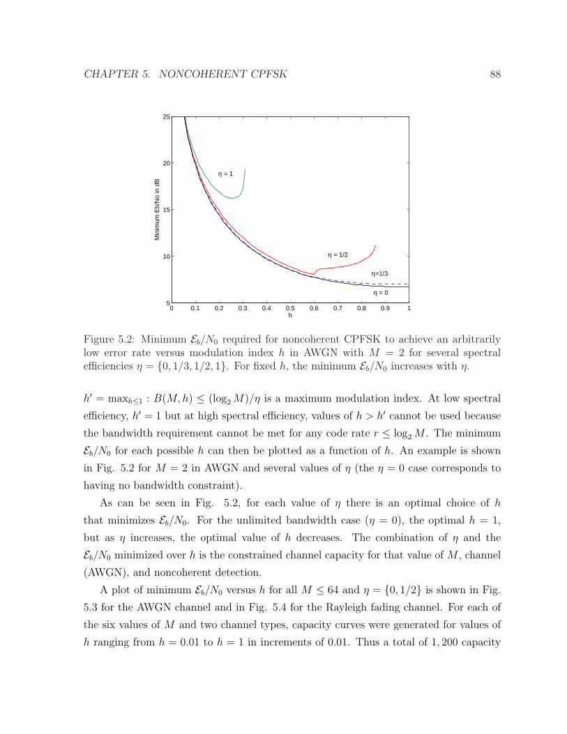
CHAPTER 5. NONCOHERENT CPFSK 88
0 0.1 0.2 0.3 0.4 0.5 0.6 0.7 0.8 0.9 15
10
15
20
25
h
Min
imum
Eb/
No
in d
B
η = 0
η=1/3
η = 1/2
η = 1
Figure 5.2: Minimum Eb/N0 required for noncoherent CPFSK to achieve an arbitrarilylow error rate versus modulation index h in AWGN with M = 2 for several spectralefficiencies η = {0, 1/3, 1/2, 1}. For fixed h, the minimum Eb/N0 increases with η.
h′ = maxh≤1 : B(M,h) ≤ (log2 M)/η is a maximum modulation index. At low spectral
efficiency, h′ = 1 but at high spectral efficiency, values of h > h′ cannot be used because
the bandwidth requirement cannot be met for any code rate r ≤ log2 M . The minimum
Eb/N0 for each possible h can then be plotted as a function of h. An example is shown
in Fig. 5.2 for M = 2 in AWGN and several values of η (the η = 0 case corresponds to
having no bandwidth constraint).
As can be seen in Fig. 5.2, for each value of η there is an optimal choice of h
that minimizes Eb/N0. For the unlimited bandwidth case (η = 0), the optimal h = 1,
but as η increases, the optimal value of h decreases. The combination of η and the
Eb/N0 minimized over h is the constrained channel capacity for that value of M , channel
(AWGN), and noncoherent detection.
A plot of minimum Eb/N0 versus h for all M ≤ 64 and η = {0, 1/2} is shown in Fig.
5.3 for the AWGN channel and in Fig. 5.4 for the Rayleigh fading channel. For each of
the six values of M and two channel types, capacity curves were generated for values of
h ranging from h = 0.01 to h = 1 in increments of 0.01. Thus a total of 1, 200 capacity

CHAPTER 5. NONCOHERENT CPFSK 89
0 0.1 0.2 0.3 0.4 0.5 0.6 0.7 0.8 0.9 10
5
10
15
20
25
30
h
Min
imum
Eb/
No
in d
B
η = 1/2 (solid lines)η = 0 (dashed lines)
M=2
4
8
16
32
64
Figure 5.3: Minimum Eb/N0 required for noncoherent CPFSK to achieve an arbitrarilylow error rate versus modulation index h in AWGN for several modulation orders M ={2, 4, 8, 16, 32, 64} and spectral efficiencies η = {0, 1/2}.

CHAPTER 5. NONCOHERENT CPFSK 90
0 0.1 0.2 0.3 0.4 0.5 0.6 0.7 0.8 0.9 10
5
10
15
20
25
30
h
Min
imum
Eb/
No
in d
B
η = 1/2 (solid lines)
η = 0 (dashed lines)M=2
4
8
16
32
64
Figure 5.4: Minimum Eb/N0 required for noncoherent CPFSK to achieve an arbitrarilylow error rate versus modulation index h in Rayleigh fading for several modulation ordersM = {2, 4, 8, 16, 32, 64} and spectral efficiencies η = {0, 1/2}.

CHAPTER 5. NONCOHERENT CPFSK 91
0 0.1 0.2 0.3 0.4 0.5 0.6 0.7 0.8 0.9 10
2
4
6
8
10
12
14
16
18
η in bps/Hz
Min
imum
Eb/
No
in d
B
M=64
M=2
M=4
M=8
M=16
M=32
Figure 5.5: Minimum Eb/N0 required for noncoherent CPFSK to achieve an arbitrarilylow error rate versus spectral efficiency η in AWGN for several modulation orders M ={2, 4, 8, 16, 32, 64}. For fixed η the minimum Eb/N0 decreases with increasing M . Thevalues at η = 0 correspond to the orthogonal FSK capacity.
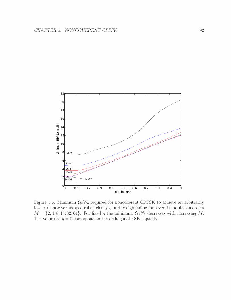
CHAPTER 5. NONCOHERENT CPFSK 92
0 0.1 0.2 0.3 0.4 0.5 0.6 0.7 0.8 0.9 10
2
4
6
8
10
12
14
16
18
20
22
η in bps/Hz
Min
imum
Eb/
No
in d
B
M=64
M=2
M=4
M=8M=16
M=32
Figure 5.6: Minimum Eb/N0 required for noncoherent CPFSK to achieve an arbitrarilylow error rate versus spectral efficiency η in Rayleigh fading for several modulation ordersM = {2, 4, 8, 16, 32, 64}. For fixed η the minimum Eb/N0 decreases with increasing M .The values at η = 0 correspond to the orthogonal FSK capacity.

CHAPTER 5. NONCOHERENT CPFSK 93
curves were generated and each curve was created using at least 2 million simulated
symbols per SNR point in the range of interest. Altogether, over 1 trillion symbols
were simulated, and it is estimated that this task would have taken about one year to
complete on a single PC computer. To speed the run time, simulations were executed on
a virtual private grid computer powered by the idle capacity of 30 workstations located
in the teaching laboratories at the Lane Department of Computer Science and Electrical
Engineering at West Virginia University.1. The entire simulation scenario took just two
weeks to complete on the grid computer.
From these curves, it can be seen that the minimum h decreases with increasing M .
Interestingly, the minimum Eb/N0 decreases with increasing M even when the bandwidth
is constrained. By finding the minimum value of Eb/N0 with respect to h for each M over
a wide range of η, one can finally determine the capacity of CPFSK. Capacity can now
be plotted in terms of spectral efficiency η versus the corresponding minimum Eb/N0,
as shown for several M and η ≤ 1 in Fig. 5.5 for AWGN and Fig. 5.6 for Rayleigh
fading. Note that the minimum Eb/N0 in dB increases roughly linearly with η. The
minimum Eb/N0 decreases with increasing M . The minimum Eb/N0 at η = 0 is achieved
with h = 1 for each M , and therefore these values are identical to the ones for orthogonal
FSK modulation given in Chapter 2. While there is a benefit to increasing M at very low
η, these benefits begin to disappear as η is increased. For both the AWGN and Rayleigh
fading channels, there is no benefit to using M > 16 for spectral efficiencies η > 0.3 since
the curves for M = {16, 32, 64} merge at these higher spectral efficiencies. Furthermore,
in AWGN the curves for M = {8, 16, 32, 64} begin to merge as η > 0.5, indicating that
there is no benefit to using M > 8 in AWGN when η > 0.5.
5.3 Multi-symbol Noncoherent Detection
Consider an N -symbol block noncoherent detector [79]. Let the block of modulated
symbols be xN−10 and the block of received symbols be yN−1
0 . The block noncoherent
detector computes the probability p(yN−10 |xN−1
0 ) for each of the MN possible xN−10 . If
1Job scheduling was performed online via the Global Grid Exchange (g2ex.com) which runs theFrontier Grid Platform developed by Parabon Computation (parabon.com).

CHAPTER 5. NONCOHERENT CPFSK 94
the initial phase φ0 at the start of the block is given, the conditional probability can be
represented by the chain rule as
p(yN−10 |xN−1
0 , φ0) =N−1∏i=0
p(yi|yi−10 ,xN−1
0 , φ0)
=N−1∏i=0
p(yi|xi, φi), (5.6)
where the second equality comes directly from the properties of Markov chains, and φi
is recursively updated using (4.2).
From (5.6) and (4.11), if the input to the modulator is q = [q0, ..., qN−1], then the
conditional pdf is
p(yN−10 |q, φ0) ∝ exp
(2
√Es
N0
Re{e−jφ0µ(q)
})(5.7)
where
µ(q) =N−1∑i=0
yqie−2hπ
∑i−1k=0 qk . (5.8)
The noncoherent detector assumes φ0 has a uniform distribution over [0, 2π). Marginal-
izing p(yN−10 |q, φ0) with respect to φ0 yields
p(yN−10 |q) ∝ I0
(2
√Es
N0
|µ(q)|)
, (5.9)
where I0(·) is the 0th order modified Bessel function of the first kind.
The capacity can then be calculated from
C(n)N = log2 M +
1
NE
log2
I0
(2√Es|µ(q)|
N0
)
∑q′∈Q
I0
(2√Es|µ(q′)|
N0
)
, (5.10)
where Q is the set of MN possible values of q and the expectation is taken over the

CHAPTER 5. NONCOHERENT CPFSK 95
-20 -15 -10 -5 0 5 10 15 200
0.2
0.4
0.6
0.8
1
Es/No
capa
city
CoherentNoncoherent N = 12Noncoherent N = 4Noncoherent N = 2Noncoherent N = 1
CoherentNoncoherent
symbol by symbolMSKM = 2, h = 1/2
Figure 5.7: Capacity of MSK using multi-symbol noncoherent and coherent detection.
ensemble of all possible transmitted q and received yN−10 . As in the coherent case, the
above expectation can be found using Monte Carlo integration.
As an example, Fig. 5.7 shows the capacity of multi-symbol noncoherent detection
of MSK for several different block sizes. The rightmost curve (N = 1) is the capacity
of symbol-by-symbol noncoherent detection, while the leftmost curve is the coherent ca-
pacity. By increasing N from 1 to 4, the gain at code-rate 0.5 is about 5 dB, and it is
only 3.5 dB worse than the coherent detection. When the block size N is larger, this
capacity of noncoherent detection gets closer to that of coherent detection. When N in-
creases to infinity, we conjecture that the noncoherent capacity converges to the coherent
capacity. This is consistent with the asymptotic capacity analysis [80, 81] and the BER
performance in [79]. More generally, the capacity of multi-symbol noncoherent detection
can be found for any arbitrary value of h, M , and N using the same methodology used
to generate the MSK curves shown in Fig. 5.7.
5.4 Code Design
In this section, we design channel codes to approach the noncoherent CPFSK capacity.
The method is very similar to the one used for code design for coherent detector. We still

CHAPTER 5. NONCOHERENT CPFSK 96
+=
= + Parallel/S
erial
D
+ CPFSK
Figure 5.8: Nonsystematic IRA coding structure. “=” corresponds to variable nodes and“+” corresponds to single parity-check nodes.
use the IRA code structure, but the difference is that the accumulator is placed between
the parity check codes and CPFSK modulator, as is shown in Fig. 5.8. The reason is
that CPFSK detector loses its recursive structure by doing noncoherent detection.
Fig. 5.9 shows the EXIT chart of MSK at Eb/N0 = 3.94dB. The outer code is designed
for coherent MSK at coding rate 0.5 [20]. Four different inner code EXIT curves are also
shown, corresponding to N = 1, 2, 4, 12 multi-symbol noncoherent detected MSK with
check node distribution ρ1 = 0.001, ρ2 = 0.999. Here, no accumulator is placed between
the parity-check codes and the MSK modulator. One can see that when N is larger, the
inner SISO can produce more extrinsic information output. However, when N is finite,
the inner EXIT curve always cross over the right side of the EXIT chart at some intercept
between 0 and 1. No matter how the outer code is designed, the EXIT curves of inner
and outer codes intersect at some point to the lower left of (1, 1). This predicts that
the decoding trajectory gets stuck at this point, and can not reach (1, 1), which usually
results in a high error floor.
By introducing the accumulator between parity check codes and CPFSK modulator,
the EXIT curve of noncoherent detector can gradually reach (1, 1). This is desirable
in the outer code optimization so that two EXIT curves can possibly form a narrow
tunnel between (0, 0) and (1, 1), leading to the successful decoding. Fig. 5.10 shows the
inner EXIT curve of N = 4 noncoherently detected MSK at Eb/N0 = 3.94dB, and the
matched outer code EXIT curve at coding rate 0.5. The optimization method is same as
the one in Section 4.5. The optimized threshold is about 0.24dB away from the N = 4
noncoherent capacity. The actual simulation of a 100, 000 uncoded bit frame reaches

CHAPTER 5. NONCOHERENT CPFSK 97
0 0.2 0.4 0.6 0.8 10
0.2
0.4
0.6
0.8
1Repetition codeCoherent design
Combined SPC, CPFSK noncoherent detection
Eb/N0 = 3.94 dBr = 0.5
MSK(M=2, h=½)
I E(i) ,I A(o)
IA(i),IE(o)N=1
N=2
N=4
N=12
Figure 5.9: EXIT curves of inner codes without accumulator
Table 5.1: Optimized codes for MSK at rate r = 0.5. For each of the coherent and multi-symbol noncoherent (N = 4) detectors, the degree distributions, capacity, and thresholdsare listed.
Coherent Noncoherent (N = 4)Variable λ3 = 0.570 λ3 = 0.414
Node λ7 = 0.365 λ5 = 0.439λ8 = 0.065 λ6 = 0.147
Check ρ1 = 0.001 ρ1 = 0.001Node ρ2 = 0.999 ρ2 = 0.999
Capacity(Eb/N0) 0.2 dB 3.7 dBThreshold(Eb/N0) 0.48 dB 3.94 dB

CHAPTER 5. NONCOHERENT CPFSK 98
0 0.2 0.4 0.6 0.8 10
0.1
0.2
0.3
0.4
0.5
0.6
0.7
0.8
0.9
1
IA(i),IE(o)
I E(i) ,I A(o)Repetition
code
Combined SPC, accumulator and
CPFSK N=4 noncoherent detection
Eb/N0 = 3.94 dBr = 0.5
MSK(M=2, h=½)
Figure 5.10: EXIT curve-matching result of N = 4 noncoherent detection of MSK
0 1 2 3 4 5
10
-410
-310
-210
-110
0
Eb/No
BER
CoherentNoncoherent N = 4
Coherent Capacity
Noncoherent N=4
Capacity
Figure 5.11: BER of MSK with rate r = 0.5 coding designed using EXIT curve-fitting.

CHAPTER 5. NONCOHERENT CPFSK 99
BER 10−5 at Eb/N0 = 4.03 dB. The capacity and optimization results are listed in Table
5.1. Also shown in the table is the capacity and optimization results of coherent MSK for
comparison. For coherent detection, the Eb/N0 required to achieve BER 10−5 is 0.63 dB,
about 0.15 dB away from the estimated threshold and 0.43 dB away from the capacity.
The BER curves are shown in Fig. 5.11.
5.5 Chapter Summary
Noncoherent demodulation is an attractive alternative to coherent demodulation. Unlike
the coherent case, the complexity of the noncoherent detector does not depend on h, which
may be any real number. This provides more design flexibility, especially in narrowband
systems that tend to require small values of h that would result in very complex coherent
detectors. Furthermore, noncoherent detection does not require knowledge of the set of
phases Φ or the initial phase, and the set of phases may evolve due to, for instance,
oscillator offsets or Doppler.
The main drawback of symbol-by-symbol noncoherent CPFSK is a very large penalty
in energy efficiency. For example, the symbol-by-symbol noncoherent capacity of MSK
at code rate r = 0.5 is 8.5 dB worse than the coherent capacity. Much of this loss
can be recovered by using multi-symbol noncoherent block detection. For instance by
performing detection over a block as small as N = 4, 5 dB of the loss relative to coherent
reception can be recovered. As in the coherent case, the capacity with multi-symbol
noncoherent block detection can be approached by using an IRA code designed with a
curve-fitting technique. However, since noncoherent demodulation destroys the memory
in the modulation, a differential precoder is required.

Chapter 6
Channel Estimation of Noncoherent
FSK
A nice property of FSK is that it can be detected noncoherently, when the phase changes
too quickly to be tracked. However, the demodulator in (2.13) or (5.3) requires knowledge
of the noise variance and the received signal amplitude. In practice, this information is not
known a priori and must be estimated at the receiver. Even for the demodulator without
CSI in (2.15) or (5.3), the SNR information and fading statistics are needed. Recently,
[82] [71] proposed a parametric free metric instead of the Bessel metric depending on
2a√ES/N0. The idea is to take the Taylor series expansion of I0(α) around α = 0.
After some manipulations, the demodulator produces the soft metric which is just the
normalized square of the channel observation. This metric has performance close to the
Bessel metric in AWGN channel. However, it induces a loss in Rayleigh fading channel
and other type of random interference channels.
In an iterative receiver, a reasonable approach is to feed back extrinsic information
from the decoder back to a channel estimator [83]. For a good overview of iterative
decoding and channel estimation, see [84] and the references therein.
It is assumed that the channel experiences block fading. Blocks of N consecutive
FSK symbols are attenuated by the same channel gain (though they could experience
different phase shifts) and are corrupted by noise that is stationary for the duration of
the block. Aside from this block fading condition, the estimator makes no assumptions
100

CHAPTER 6. CHANNEL ESTIMATION OF NONCOHERENT FSK 101
regarding the statistics of the channel. Both the received fading amplitude and the noise
spectral density are estimated because either one or both could change from block-to-
block due to jamming, interference, or other environmental conditions. The estimator
itself is derived using the expectation maximization (EM) algorithm [85], which iteratively
finds the maximum likelihood (ML) estimate even though an explicit form is not readily
achievable when extrinsic information is fed back to the estimator from the decoder.
EM-based estimator is derived in Section 6.1. Complexity reduction techniques are
discussed in Section 6.2 and simulation results given in 6.3. Section 6.4 discusses the
algorithmic complexity, and a summary of this chapter is given in Section 6.5.
6.1 Channel Estimator
6.1.1 Iterative Decoding, Demodulation and Channel Estima-
tion
The channel estimator uses Y and a priori information fed back to it from the decoder
to produce the ratio γ` = B`/A` of channel estimates for the `th block, where A and B
are defined in Section 2.1.2. The demapper and decoder exchange extrinsic information
in a turbo-processing loop, just like the perfect CSI case in Chapter 2. The demapper
output is a m by Nq matrix Z whose (k, i)th element is
zk,i = logp(bk,i = 1|yi, γbi/Nc,vi\vk,i)
p(bk,i = 0|yi, γbi/Nc,vi\vk,i)(6.1)
= log
∑
q∈Q(1)k
I0
(γbi/Nc|yq,i|
) m−1∏j=0j 6=k
exp (bj(q)vj,i)
∑
q∈Q(0)k
I0
(γbi/Nc|yq,i|
) m−1∏j=0j 6=k
exp (bj(q)vj,i)
(6.2)
where vi is the ith column of V, a m by Nq matrix output by the SISO decoder. The
conditioning in vi\vk,i implies that the extrinsic information for bit bk,i is produced

CHAPTER 6. CHANNEL ESTIMATION OF NONCOHERENT FSK 102
without using vk,i. The (k, i)th element of V is
vk,i = logp(bk,i = 1|Z\zk,i)
p(bk,i = 0|Z\zk,i). (6.3)
which is derived for SISO decoders in [35].
6.1.2 EM Channel Estimator
The channel estimator works on a block by block base. Since the block estimation is
independent, we temporarily drop the block index `. Following the conditional probability
in (5.3), we have
p(yi|qi = ν, a, ES, N0)
=1
πMNM0 |K|
exp
(−yH
i K−1yi + a2ES
N0
)I0
(2a√ES|yν,i|
N0
), (6.4)
The log-likelihood function with respect to ES, N0 and d can be represented as
L = log [p(Y|A,B,q)]
= −MN ln A− C
A− NB2
4A+
N−1∑i=0
ln I0
(B |yqii|
A
), (6.5)
where A = N0, B = 2a√ES and C =
∑i y
Hi K−1yi. C can be viewed as the decoupled
energy, and for the orthogonal case h = 1, C =∑
k,i |yki|2.The representation of (6.5) includes the unknown parameter q. This information is
never known to the receiver before the perfect decoding. However the extrinsic informa-
tion V from the decoder can be used as the priori of q. In order to find the ML solution,
we need to sum over all possibilities of q, by using the extrinsic information feedback

CHAPTER 6. CHANNEL ESTIMATION OF NONCOHERENT FSK 103
from the decoder. This results in
L = logN−1∏i=0
p(yi|A,B)
=N−1∑i=0
[log
M−1∑
k=0
p(yi|A,B, qi = k)p(qi = k)
]. (6.6)
Even though the expression can be broken down to the product of independent symbols,
the argument of the log function still contains the summation of M terms, and therefore
a direct solution is too complex to be practical.
Although a direct maximum-likelihood estimation is impractical, the EM algorithm
is an appropriate iterative approach to estimating {A, B} [85]. Let {Y,q} denote the
complete data set, which using (6.4) has log-likelihood
L(A,B) = log p(Y,q|A,B)
= log p(Y|A,B,q) + log p(q)
∼ −MN log A− C
A− NB2
4A
+N−1∑i=0
log I0
(B |yqi,i|
A
), (6.7)
where ∼ is used to indicate that the quantities are equal up to irrelevant quantities that
do not affect the maximization, namely the terms −NM log π and log p(q).
Let ξ denote the EM iteration and A(ξ), B(ξ) denote the estimates of A,B after the
ξth iteration. Iteration ξ starts with the E-step
Q(A,B) = Eq|Y,A(ξ−1),B(ξ−1) [L(A,B)] (6.8)
where the expectation is taken with respect to the unknown symbols d conditioned on Y
and the estimates A(ξ−1), B(ξ−1) from the last EM iteration. Substituting the likelihood

CHAPTER 6. CHANNEL ESTIMATION OF NONCOHERENT FSK 104
function (6.7) into (6.8) yields
Q(A,B) = −MN log A− C
A− NB2
4A+
N−1∑i=0
M−1∑
k=0
p(ξ−1)k,i log I0
(B |yk,i|
A
)(6.9)
where
p(ξ−1)k,i = p(qi = k|yi, A
(ξ−1), B(ξ−1))
=p(yi|qi = k, A(ξ−1), B(ξ−1))p(qi = k)
p(yi|A(ξ−1), B(ξ−1)). (6.10)
The last step uses the fact that q is independent of A and B. Applying (2.13), we obtain
p(ξ−1)k,i = α
(ξ−1)i I0
(B(ξ−1)|yk,i|
A(ξ−1)
)p(qi = k) (6.11)
where α(ξ−1)i is the normalization factor forcing
∑M−1k=0 p
(ξ−1)k,i = 1, i.e.
α(ξ−1)i =
1∑M−1
k=0 I0
(B(ξ−1)|yk,i|
A(ξ−1)
)p(qi = k)
(6.12)
and p(qi = k) is found from the a priori input vi using [86]
p(qi|vi) =
µ−1∏j=0
evj,ibj(qi)
1 + evj,i. (6.13)
The M-step is
A(ξ), B(ξ) = arg maxA,B
Q(A,B) (6.14)
which, can be found by setting the derivatives of the function Q(A,B) with respect to A

CHAPTER 6. CHANNEL ESTIMATION OF NONCOHERENT FSK 105
and B to zero. The solution to the corresponding system of equations is
A(ξ) =1
MN
(C − N(B(ξ))2
4
)(6.15)
B(ξ) =2
N
N−1∑i=0
M−1∑
k=0
p(ξ−1)k,i |yk,i|F
(4MNB(ξ)|yk,i|4C −N(B(ξ))2
)(6.16)
where F (x) = I1(x)/I0(x). While a closed form solution to (6.16) is difficult to obtain,
it can be found recursively [87].
To select an initial estimate for B prior to the first BICM-ID iteration, consider that in
the absence of noise, yk,i = a√ESδk,qi
ejθi , which has a magnitude of either |yk,i| = a√ES
(when k = qi) or |yk,i| = 0 (otherwise). Thus, an estimate for a√ES = B/2 can be
achieved by taking the maximum |yk,i| over any column of Y. To account for noise, the
average could be taken across all columns in the block, resulting in
B(0) =2
N
N−1∑i=0
maxk|yk,i| . (6.17)
The initial estimate of A is found from B(0) by evaluating (6.15) for ξ = 0. After the
initial values A(0) and B(0) are calculated, the initial probabilities {p(0)k,i} are calculated
using (6.11) with p(qi = k) = 1/M for all i and k. Next, B(1) is found by recursively
solving (6.16). Once the recursion is complete, A(1) can be directly found from (6.15),
which finalizes the first EM iteration. The second EM iteration then starts by calculating
p(1)k,i using (6.11) with p(qi = k) = 1/M and the newly acquired A(1) and B(1), and the
remaining steps are identical to the first EM iteration. The EM estimator will continue
to iterate until some stopping criterion is reached. In our simulations, we halted the
EM algorithm when the value of the estimate of B changed less than 10%, when the
estimate of B became very close to zero, or when a maximum number of 20 iterations
was reached. After the first BICM-ID iteration, the final value of B(ξ) from the previous
BICM-ID iteration can be used as the initial estimate of B, and the value of p(qi = k)
in (6.11) is found from the decoder output using (6.13).

CHAPTER 6. CHANNEL ESTIMATION OF NONCOHERENT FSK 106
6.2 Reduced Complexity Estimation
A major drawback of the proposed EM-based estimator is its complexity. In this section,
two techniques are proposed for reducing the complexity of the algorithm. One involves
a linear approximation to the F (·) function, while the other involves the hard limiting of
pk,i.
6.2.1 Linear Approximation of F (·)During each iteration of the full-complexity EM algorithm, B(ξ) is found by recursively
solving (6.16). For each step in the recursion, the nonlinear function F (x) = I1(x)/I0(x)
must be evaluated for each of the MN entries in the Y matrix, presumably by a table
look-up. The number of required table look-ups can be drastically reduced by performing
a first-order Taylor series expansion of F (x) about the point x = t, resulting in F (x) =
F (t) + F ′(t)(x − t). The expansion point t is the approximate maximum value of the
argument of F (·) in (6.16). Setting |yk,i| ≈ a√ES and C ≈ N(a2ES + MN0), we obtain
t ≈ 2a2ES/N0 = B2/(2A).
The linear approximation of the F (·) function is illustrated in Fig. 6.1. As shown,
F (x) is a monotonically increasing function with respect to x and is concave, approaching
1 when x →∞. Because the curve becomes flat when x is reasonably large, such a linear
approximation is reasonable. Assuming 4C >> N(B(ξ))2 and substituting the linear
expansion of F (·) about the point t = (B(ξ−1))2/(2A(ξ−1)) into (6.16) yields
B(ξ) ≈ [F (t)− tF ′(t)]∑N−1
i=0
∑M−1k=0 p
(ξ−1)k,i |yk,i|
N(
12− M
CF ′(t)
∑N−1i=0
∑M−1k=0 p
(ξ−1)k,i |yk,i|2
)
(6.18)
where F ′(t) = 1− F (t)t− F 2(t), as implied by equation (8.486) of [88].
With this approximation, (6.16) is replaced with (6.18), and now only a single table
look-up is required per EM iteration, instead of the MN look-ups in (6.16). Due to the
linearization, B(ξ) can be found directly from (6.18) without requiring a recursion, which
greatly simplifies the algorithm. Notice, however, that the expansion point t(q−1) must

CHAPTER 6. CHANNEL ESTIMATION OF NONCOHERENT FSK 107
0 1 2 3 4 5 6 7 8 9 100
0.5
1
1.5
x
F(x
)Linear
Approximation
( t , F(t) )
Figure 6.1: F (x) = I1(x)/I0(x) and its linear approximation.
be changed after each EM iteration.
The linear approximation of F (x) is tight when the expansion point is sufficiently large
and the argument of F (·) in the original EM equation (6.16) is close to the expansion
point. Since the expansion point is proportional to the estimated SNR, the approximation
gets worse with decreasing SNR. Because of the concavity of the F (·) function, the
approximation will overestimate its value, leading to an overestimation of B. However,
overestimating B is better than underestimating it, which agrees with observations made
in [89] that the SNR can be overestimated in an AWGN channel by as much as 3 dB
without significantly harming the performance of a turbo code. Even when the expansion
point is sufficiently high, the approximation will be loose when the arguments in the
linearized F (·) function are small, which occurs for those values of |yk,i| that are small.
Small values of |yk,i| occur more frequently at high SNR, since the M − 1 entries of
each vector yi that do not pertain to the transmitted symbol would all be small. While
the linear approximation is indeed poor for these small values of |yk,i|, this problem is

CHAPTER 6. CHANNEL ESTIMATION OF NONCOHERENT FSK 108
mitigated by the fact that every |yk,i| is weighted by its corresponding probability pk,i,
which will also be small. Thus, the contribution of the small values of |yk,i| to the overall
estimate is negligible, and the poor approximation at these values does not seriously
harm overall performance.
6.2.2 Hard Limiting of pk,i
During the ξth iteration of the full-complexity EM algorithm, each pk,i must evaluated
using (6.11). For each symbol, the normalization factor αi must also be calculated to
assure that∑M−1
k=0 pk,i = 1. The normalization factor can be avoided by setting pk,i = 1
for one particular value of k, denoted k0, and setting pk,i = 0 for all k 6= k0. The index
k0 should be the value of k that maximizes (6.11). Taking the logarithm of (6.11), which
does not change the maximization, and using (6.13) for p(qi = k) results in
k0 = arg maxk
log
[I0
(B(ξ−1)|yk,i|
A(ξ−1)
)]+
µ−1∑j=0
vj,ibj(k).
(6.19)
In addition to eliminating the need for computing the normalization factor αi, this
approximation has the additional benefit of eliminating the exponential functions in
(6.13). Complexity is further reduced when B is calculated with either (6.16) or (6.18)
because those terms for which pk,i = 0 do not need to be considered, and therefore the
summations over k are eliminated. Another benefit of this method is that it provides
a natural stopping criterion for the EM algorithm, which should halt once the pk,i’s no
longer change from one iteration to the next.
While (6.19) is a very coarse approximation to (6.11) in the normal EM algorithm,
it still uses both the decoder’s a priori information as well as the channel likelihood
based on the current estimates. This approximation tends to make (6.16) overestimate
the value of B, but the performance loss due to this approximation is small, as will be
demonstrated in the next section.

CHAPTER 6. CHANNEL ESTIMATION OF NONCOHERENT FSK 109
6.3 Simulation Results
To illustrate the performance of the proposed estimators, a set of simulations were run.
Note that all the results shown in this chapter are based on orthogonal FSK systems.
Since the only difference between the estimators in orthogonal and nonorthogonal FSK
systems lie in the energy calculation C, as is mentioned in Section 6.1.2, we only show
the results of coded orthogonal FSK systems in this chapter. In the next chapter, the
estimator is also applied to nonorthogonal CPFSK used in the frequency hopping appli-
cation.
The simulated system uses the turbo code from the cdma2000 specification [15] and
16-FSK modulation. The specific turbo code that was selected is a rate-1/2 code with
Nu = 1530 input bits. As the cdma2000 standard requires 12 coded tail bits, the length
of each code word is actually Nb = 2(1530) + 12 = 3072 bits or Nd = 768 FSK symbols.
The receiver executed up to 20 BICM-ID iterations. A perfect CRC check was assumed
in the simulations, so that the iterations would stop once the data is correctly decoded.
Fig. 6.2 shows the bit error rate (BER) performance of five systems over a Rayleigh
block fading channel with N = 4 symbols per block. The curve with the best performance
corresponds to the case that a√ES and N0 are known by the receiver. While not possible
in practice, this curve serves as a benchmark. The other curves correspond to four
implementations of the proposed estimator. The best performing estimator is the full-
complexity EM-based estimator. The other curves correspond to the reduced complexity
techniques described in Section 6.2. In order from best-to-worst performing, the curves
use the following complexity reduction techniques: (1) Hard limiting of pk,i (EM-H); (2)
Linear approximation of the F (·) function (EM-L); and (3) Both Hard limiting of pk,i
and a linear approximation of F (·) (EM-H/L). For this example, the full-complexity EM
estimator has a 0.55 dB loss relative to the system with known a√ES and N0. The
additional loss due to the complexity reduction techniques is about 0.05 dB for EM-H,
0.1 dB for EM-L, and 0.15 dB for EM-H/L.
Fig. 6.3 shows BER results in Rayleigh block fading for several values of block length
N . For each value of N , two curves are shown. The curve on the left (dashed line) is
for the case that a√ES and N0 are known by the receiver, while the curve on the right

CHAPTER 6. CHANNEL ESTIMATION OF NONCOHERENT FSK 110
4.5 5 5.5 6 6.5 7 7.510
−5
10−4
10−3
10−2
10−1
100
Eb/No(dB)
BER
EM−H/L
EM−L
EM−H
EM
Known a2
Es and No
Figure 6.2: BER comparison of the different estimators in block Rayleigh fading with N =4 symbols per block. The system uses 16-FSK modulation and the rate 1/2 cdma2000turbo code (Nu = 1530 input bits). Shown from left to right is performance with:(1) a
√ES and N0 known for each block; (2) The full-complexity EM estimator; (3)Estimator EM-H, which makes hard decisions on pk,i; (4) Estimator EM-L, which usesa linear approximation to the F (·) function; and (5) Estimator EM-H/L, which makeshard decisions on pk,i and uses a linear approximation to F (·).
shows performance of Estimator EM-H/L. As the value of N decreases, performance of
both systems improves due to increasing diversity. However, the gap between the two
curves widens with decreasing N due to increasing estimation error. Results were also
produced for N = 1 (not shown to keep the plot uncluttered), but the performance of
the EM-H/L estimator with N = 1 is about 0.5 dB worse than when N = 4 and nearly
2 dB worse than when a√ES and N0 are known.
To better illuminate the effect of block length on estimator performance, Fig. 6.4
shows simulation results for the same cdma2000 turbo code and 16-FSK in an unfaded,
AWGN channel. While the fading is a constant a = 1, the estimator runs assuming a
block length of N symbols. When N = 4, the performance of the estimator is about 0.3
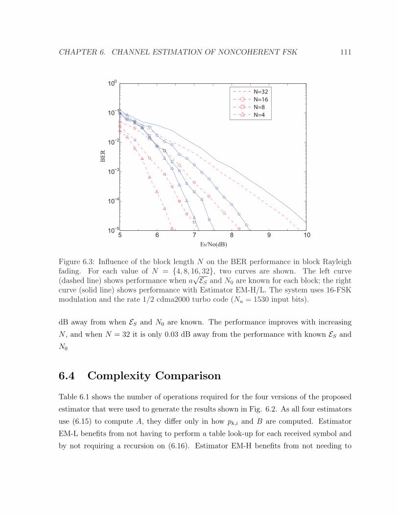
CHAPTER 6. CHANNEL ESTIMATION OF NONCOHERENT FSK 111
5 6 7 8 9 10
N=32
N=16
N=8
N=4
Eb/No(dB)
BER
10−5
10−4
10−3
10−2
10−1
100
Figure 6.3: Influence of the block length N on the BER performance in block Rayleighfading. For each value of N = {4, 8, 16, 32}, two curves are shown. The left curve(dashed line) shows performance when a
√ES and N0 are known for each block; the rightcurve (solid line) shows performance with Estimator EM-H/L. The system uses 16-FSKmodulation and the rate 1/2 cdma2000 turbo code (Nu = 1530 input bits).
dB away from when ES and N0 are known. The performance improves with increasing
N , and when N = 32 it is only 0.03 dB away from the performance with known ES and
N0
6.4 Complexity Comparison
Table 6.1 shows the number of operations required for the four versions of the proposed
estimator that were used to generate the results shown in Fig. 6.2. As all four estimators
use (6.15) to compute A, they differ only in how pk,i and B are computed. Estimator
EM-L benefits from not having to perform a table look-up for each received symbol and
by not requiring a recursion on (6.16). Estimator EM-H benefits from not needing to

CHAPTER 6. CHANNEL ESTIMATION OF NONCOHERENT FSK 112
2.6 2.8 3 3.2 3.4 3.6
N=4
N=8
N=16
N=32
known Es and No
10−5
10−4
10−3
10−2
10−1
100
Eb/No(dB)
BER
Figure 6.4: Performance in AWGN as a function of block length N . The performance withknown ES and N0 (dashed lines) is compared against the performance with EstimatorEM-H/L. Modulation is 16-FSK. The code is the rate 1/2 cdma2000 turbo code withNu = 1530.
compute the normalization factor (6.12), by computing (6.13) in the log-domain, and not
needing to sum over k in (6.16). EM-L/H combines the benefits of EM-L and EM-H.
The overall complexity also depends on the average number of EM iterations per
BICM-ID iteration. For the simulation that produced the BER results shown in Fig.
6.2, the average number of full EM iterations (per BICM-ID iteration) was approximately
1.1 for EM-H, 1.4 for both EM and EM-L/H, and 1.5 for EM-L. These values are small
primarily as a consequence of the loose stopping criterion for the EM algorithm (if B
changes less than 10%, it will halt). A tighter stopping criterion (e.g. halting when B
changes less than 1%) will induce more EM iterations (about 3 for the EM estimator), but
will not significantly improve the BER performance. Longer blocks generally required
fewer iterations, on average. The higher value for EM-L suggests that the approximation
for F (·) caused it to converge more slowly.

CHAPTER 6. CHANNEL ESTIMATION OF NONCOHERENT FSK 113
Table 6.1: Number of operations required for each type of estimator to execute one EMiteration per block of N symbols. M is the modulation order and R is the number ofrecursions used to solve (6.16).
(a) Operations required to compute pk,i
Algorithm Additions Multiplications Look-Ups
EM N(M − 1) 3NM NMEM-L N(M − 1) 3NM NMEM-H MN MN MN
EM-L/H MN MN MN
(b) Operations required to compute B.Algorithm Additions Multiplications Look-Ups
EM RNM NM + R(2NM + 5) RNMEM-L 2(NM − 1) + 4 2MN + 7 1EM-H RN R(2N + 5) RM
EM-L/H 2(N − 1) + 4 3N + 7 1
In addition to counting operations, another way to assess complexity is to count CPU
cycles in an actual implementation. We did this for the four estimators (implemented in
the C language) during the simulation that produced Fig. 6.2. As expected, the original
EM estimator required the most CPU cycles, and in fact required more than that used
for the turbo decoder. Estimator EM-L had a complexity of about 1/4 that of Estimator
EM, making it only a little more complex than the demapper. Estimator EM-L/H is 1/3
the complexity of Estimator EM-L, making its complexity negligible compared to the
decoder and demapper. Given the slight loss in performance, Estimator EM-L/H is an
attractive solution.
6.5 Chapter Summary
The proposed robust noncoherent system has been shown to withstand the severe chan-
nel conditions of fast fading, unknown fading attenuation, unknown fading statistics, and
unknown noise-power spectral density. The channel-state estimator is based on the Ex-
pectation Maximization algorithm and exploits extrinsic information produced after each
decoding iteration of the turbo code. Each updated channel-state estimate is applied to

CHAPTER 6. CHANNEL ESTIMATION OF NONCOHERENT FSK 114
the next decoder iteration. Simulation results indicate that if the fading coherence time
exceeds four channel symbols, then the performance is close to what could be obtained
with perfect channel-state information. Although the estimator using the exact EM al-
gorithm has a high complexity, the linear approximation of F (·) and the hard limiting of
pk,i can be applied to reduce the complexity with minor loss in BER performance.

Chapter 7
Application of CPFSK to Frequency
Hopping Networks
Spread Spectrum (SS) is a technique involving the transmission of information over a
bandwidth larger than the data rate. This technique has the advantage of resisting
narrowband interference and supporting multiuser access simultaneously on the same
band, known as code division multiple access (CDMA). There are two different types
of SS, direct sequence SS (DSSS) and frequency hopping SS (FHSS). In DSSS, each
user’s signal is multiplied by a spreading sequence, resulting in a larger bandwidth than
the original signal. The DSSS technique is now widely used in many systems, such
as wideband CDMA (WCDMA) [90], CDMA2000 system [15], IEEE 802.11b wireless
local area networks (WLANs) [91] and IEEE 802.15.4 wireless personal area networks
(WPANs) [92], also known as ZigBee. In FHSS, the total band is divided into a number
of frequency channels. Each user transmits its signal through a single frequency channel
at a time, but periodically changes the frequency channel in a pseudorandom fashion.
One popular application of FHSS is the Bluetooth system [93].
In Section 7.1, we introduce frequency hopping (FH) networks by showing a simple
example using capacity approaching Gaussian signaling. From this simple example, we
show that there is a fundamental tradeoff between the number of frequency channels
and the bandwidth per channel. Given a fixed bandwidth, increasing the number of
frequency channels reduces the probability of interference, but leads to lower data rate
115

CHAPTER 7. APPLICATION OF CPFSK TO FH NETWORKS 116
due to the smaller bandwidth per channel. Decreasing the number of frequency channels
induces more interference but offers higher data rate. by showing the tradeoff between
the number of frequency channels and and discuss its throughput under multiple access
interference. From Section 7.2, we use noncoherent CPFSK in FH networks, whose
parameters are optimized using the results given in Section 5.2. The performances of
the designed systems under partial band jamming and multiple access interferences are
evaluated in Section 7.3 and Section 7.4, respectively.
7.1 Frequency Hopping Networks
Recently, [94] showed that in wireless ad hoc networks, FHSS is superior to DSSS in terms
of transmission capacity, which reinforced the early work by Pursley and Taipale [95],
who studied SS systems from the perspective of error rate. While FH-CDMA and DS-
CDMA could have identical or close performance in cellular systems assuming perfect
power control, such assumption is impossible in wireless ad hoc networks because of
the random locations of the transmitters and receivers. When the path loss exponent is
greater than 2, which is always true in practice, it is better to avoid interference with
FHSS rather than suppressing the interference with DSSS. Here, the path loss exponent
α means that the transmission power decays at at rate of dα, where d is the distance to
the transmitter. Although the transmission capacity defined in [94] allows the outage
probability to be nonzero, the outage threshold is set to an arbitrary fixed number,
and the rate and the number of frequency channels are not optimized. We consider a
simple FH network, where each user transmits a capacity-approaching Gaussian signal.
The throughput is optimized over the transmission rate and the number of frequency
channels.
In this example, we consider J transmitters and only one receiver. The receiver can
hear its desired transmitter, and the other J−1 transmitters as well. The total spectrum
available to the network occupies a bandwidth of W , and it is equally divided into Q
frequency channels, each with probability 1/Q being selected by a particular transmitter.
Although path loss is not considered in this simple example, each of the J received signals
experience independent Rayleigh fading, i.e. the transmitted symbol is multiplied by a

CHAPTER 7. APPLICATION OF CPFSK TO FH NETWORKS 117
fading gain drawn from a complex Gaussian distribution with zero mean and variance
1/2 on both dimensions. The average received signal to noise ratio (SNR) is assumed to
be same for the desired signal and the J − 1 interfering signals.
It is straightforward to see that the probability of each interfering transmitter selecting
the same frequency channel as the desired transmitter is 1/Q. As a result, the probability
of n interfering signals colliding with the desired signal is,
Pc[n] =
(J
n
)(1
Q
)n (1− 1
Q
)J−n
. (7.1)
Assuming each transmitter uses capacity-approaching Gaussian signalling, the outage
probability is defined as
PO , Pr
[W
Qlog2 (1 + SINR) < R
], (7.2)
where SINR is the signal to interference and noise ratio. The left side of the inequality
can be viewed as Gaussian capacity spanning 2W/Q dimensions [7]. Using the theorem
on total probability, the outage probability can be expressed as,
PO =J−1∑n=0
Pr
[W
Qlog2 (1 + SINR) < R
∣∣∣∣ n
]Pc[n]. (7.3)
The SINR with n interfering signals is
SINR =Pa2
0
N0WQ
+∑n
i=1Pa2i
, (7.4)
where P is the power of the transmitter, a0 is the fading amplitude of the desired signal,
and ai’s are those of the interference signals.
When the fading coefficients are independent and identically distributed (i.i.d.) Rayleigh,
the outage probability given n interference signals is shown in Appendix A to be
Pr
[W
Qlog 2 (1 + SINR) < R
∣∣∣∣n
]= 1− exp
[−WN0
QP (2RQ/W − 1)
]2−nQR/W . (7.5)

CHAPTER 7. APPLICATION OF CPFSK TO FH NETWORKS 118
Substituting (7.5) and (7.1) back into (7.3), we get
PO = 1− exp
[−WN0
QP (2RQ/W − 1)
](Q− 1 + 2−RQ/W
Q
)J−1
. (7.6)
Thus, the throughput of the desired transmission is
T = R(1− PO), (7.7)
which could be achieved by hybrid automatic repeat request (ARQ) protocol [96]. A
more meaningful metric would be the throughput efficiency T/W . Letting P = REb and
defining the normalized transmission rate r = R/W , the throughput efficiency can be
written as
T
W= r exp
(− N0
QrEb
(2Qr − 1)
)(Q− 1 + 2−Qr
Q
)J−1
. (7.8)
Given J and Eb/N0, the throughput efficiency can be maximized over r and Q. The
optimization step is not given in this section. Instead, we show in Fig. 7.1 the throughput
efficiency at Eb/N0 = 3dB and J = 20 transmitters. The optimal throughput efficiency
is around 0.024 bits/s/Hz, and it is achieved at Q = 14 and r = 0.124 bits/s/Hz.
7.2 CPFSK-FH Networks
Frequency hopping with coded binary orthogonal FSK has been examined in [97]. To
improve the energy efficiency, the modulation alphabet size M can be increased. However,
this comes at the expense of a decrease in the bandwidth efficiency. Given a fixed
bandwidth W , the number of frequency channels is reduced, which makes the system more
vulnerable to both multiple access frequency hopping signals and multitone jamming [33].
Aiming at reducing the bandwidth of each channel without losing much performance, we
consider frequency hopping using the nonorthogonal FSK discussed in Chapter 5. [45]
and [98] analyzed frequency hopping with M-ary PSK, iterative decoding, and channel
estimation. The proposed system with noncoherent, nonorthogonal CPFSK has the

CHAPTER 7. APPLICATION OF CPFSK TO FH NETWORKS 119
00.1
0.20.3
0.4
0
10
20
300
0.005
0.01
0.015
0.02
0.025
r (bits/s/Hz)Q
T/W
(bi
ts/s
/Hz)
Figure 7.1: Throughput Efficiency of FH network in Rayleigh fading environment,Eb/N0 = 3dB, J = 20 transmitters
following primary advantages relative to the existing systems with differential detection
or orthogonal modulation.
1. No extra reference symbol and no estimation of the phase offset in each dwell
interval are required.
2. It is not necessary to assume that the phase offset is constant throughout a dwell
interval.
3. The channel estimators are much more accurate and can estimate an arbitrary
number of interference and noise spectral density levels.
4. The compact spectrum during each dwell interval allows more frequency channels
and, hence, enhances performance against multiple-access interference and multi-
tone jamming.
From Fig. 5.3 and 5.4, we can see a gain by increasing the modulation alphabet size
M even when there is a bandwidth limit. However, when M > 8, such gain diminishes,

CHAPTER 7. APPLICATION OF CPFSK TO FH NETWORKS 120
but the receiver complexity increases rapidly. Therefore, we limit our choice of M to be
4 and 8.1
For M = 4 in Fig. 5.4, h = 0.46 is the approximate optimal value when BmaxTu = 2,
and the corresponding coding rate is approximately r(o) = 16/27. For M = 8, h = 0.32
is the approximate optimal value when BmaxTu = 2 and the corresponding code rate is
approximately r(o) = 8/15. At the optimal values of h, the plots indicate that the loss
is less than 1.5 dB for the AWGN channel and less than 3 dB for the Rayleigh channel
relative to what could be attained with the same value of M , h = 1 (orthogonal CPFSK),
and an unlimited bandwidth.
7.3 Partial Band Jamming
Simulation experiments were conducted to assess the performance of frequency hopping
systems with 4-ary CPFSK and 8-ary CPFSK under the bandwidth constraint BmaxTu =
2. The approximate optimal values of h and R determined from the bandwidth constraint
and information theory are used. The interfering signal is modelled as partial-band noise
interference that introduces It0/µ additional interference spectral density in an interfered
frequency channel, where µ is the fraction of the hopping band with interference and It0
is the spectral density when µ = 1. Thus, the total interference power is conserved as
µ varies. The simulated system uses the turbo code from the UMTS specification [16]
with 2048 information bits and the specified code rate matching algorithm. The receiver
executes no more than 20 iterations, as an early halting routine stops the iterations once
the data is correctly decoded. The figures display the minimum value of Eb/N0 necessary
to obtain a bit error probability equal to 10−3 versus µ for Rayleigh fading, Rician fading
with factor K = 10dB, and the AWGN channel. A block coincides with a dwell interval,
and the parameter A, previously defined as the noise spectral density N0 in Section 2.1.2,
now represents the spectral density due to the noise and the interference during a dwell
interval. The symbols of a dwell interval undergo the same fading amplitude, and the
1For a given h, M = 4 FSK performs better than M = 2 FSK, while the bandwidths of the twosystems are roughly the same.

CHAPTER 7. APPLICATION OF CPFSK TO FH NETWORKS 121
µ
Eb/N
o (
dB
)
Rayleigh
Rician K = 10dB
AWGN
0 0.2 0.4 0.6 0.8 15
10
15
20
25
EM estimation
Perfect CSI
Figure 7.2: Minimum Eb/N0 required for frequency hopping system to achieve BER at10−3 versus fraction of partial band interference µ, Eb/It0 = 10dB, 32 hops per codeword,4-ary CPFSK, h = 0.46, Rayleigh fading, Rician fading K = 10dB, AWGN channel fromtop to bottom. UMTS turbo code is used, with Nu = 2048 information bits and rater(o) = 16/27.
fading amplitudes are independent from block to block, which models the frequency-
selective fading that varies after each hop. The bandwidth is assumed to be sufficiently
small that the fading is flat within each frequency channel.
Fig. 7.2 and 7.3 plot the results for 4-ary CPFSK and 8-ary CPFSK, respectively,
when there are 32 hops per codeword and 64 information bits per hop, and Eb/It0 = 10dB.
For 4-ary CPFSK, there are 3456 code bits in a codeword, 108 code bits per hop, and
54 code symbols per hop. For 8-ary CPFSK, there are 3840 code bits in a codeword,
120 code bits per hop, and 40 code symbols per hop. For 4-ary CPFSK, h = 0.46 and
R = 16/27, whereas for 8-ary CPFSK, h = 0.32 and R = 8/15. Comparison of these
two figures indicates that 8-ary CPFSK has a nearly 2 dB advantage in Eb/N0 relative to
4-ary CPFSK for Rician fading and AWGN, and much more for Rayleigh fading. Both

CHAPTER 7. APPLICATION OF CPFSK TO FH NETWORKS 122
µ
Eb
/No (
dB
)
Rayleigh
Rician K = 10dB
AWGN
0 0.2 0.4 0.6 0.8 15
10
15
20
25
EM estimation
Perfect CSI
Figure 7.3: Minimum Eb/N0 required for frequency hopping system to achieve BER at10−3 versus fraction of partial band interference µ, Eb/It0 = 10dB, 32 hops per codeword,8-ary CPFSK, h = 0.32, Rayleigh fading, Rician fading K = 10dB, AWGN channel fromtop to bottom. UMTS turbo code is used, with Nu = 2048 information bits and rater(o) = 8/15.
figures indicate that µ = 1 or interference over the entire hopping band is the worst case
for Rayleigh and Rician fading. For the AWGN channel, a smaller value of µ is worst.
The use of the EM channel estimators is shown to produce a negligible loss relative to
noncoherent detection with perfect CSI.
If the hop rate increases, the increase in the number of independently fading dwell
intervals per codeword implies that more diversity is available in the processing of a
codeword. However, the shortening of the dwell interval makes the channel estimation
less reliable by providing the estimator with fewer samples. Fig. 7.4 and 7.5 show the
results for 4-ary CPFSK and 8-ary CPFSK, respectively, when the hop rate is varied
so that there are 16, 32, or 64 hops per codeword. Independent Rayleigh fading occurs
during each dwell interval, Eb/It0 = 13dB, and the information bit rate is maintained.

CHAPTER 7. APPLICATION OF CPFSK TO FH NETWORKS 123
µ
Eb/N
o (
dB
)
16 hops,
8 coded symbols/hop
32 hops,
54 coded symbols/hop
64 hops,
27 coded symbols/hop
0 0.2 0.4 0.6 0.8 110
15
20
25
EM estimation
Perfect CSI
Figure 7.4: Minimum Eb/N0 required for frequency hopping system to achieve BER at10−3 versus fraction of partial band interference µ, Eb/It0 = 13dB, Rayleigh fading, 4-aryCPFSK(M = 4), h = 0.46, 16,32,64 hops per codeword from top to bottom. UMTSturbo code is used, with Nu = 2048 information bits and rate r(o) = 16/27.
For 4-ary CPFSK, there are N = 108, 54, or 27 code symbols per hop. For 8-ary CPFSK,
there are N = 80, 40, or 20 code symbols per hop. For 4-ary CPFSK, h = 0.46 and
R = 16/27, whereas for 8-ary CPFSK, h = 0.32 and R = 8/15. Comparison of these
two figures indicates that for Rician fading and AWGN, 8-ary CPFSK maintains its
nearly 2 dB advantage in Eb/N0 relative to 4-ary CPFSK. Despite the slow decline in the
accuracy of the EM channel estimates, the diversity improvement is sufficient to produce
an improved performance as the hop rate increases.
7.4 Asynchronous Multiple Access Interference
Multiple-access interference may occur when two or more frequency-hopping signals share
the same physical medium or network, but the hopping patterns are not coordinated. A

CHAPTER 7. APPLICATION OF CPFSK TO FH NETWORKS 124
µ
Eb/N
o (
dB
)
16 hops,
80 coded symbols/hop
32 hops,
40 coded symbols/hop
64 hops,
20 coded symbols/hop
0 0.2 0.4 0.6 0.8 110
15
20
25
EM estimation
Perfect CSI
Figure 7.5: Minimum Eb/N0 required for frequency hopping system to achieve BER at10−3 versus fraction of partial band interference µ, Eb/It0 = 13dB, Rayleigh fading, 8-aryCPFSK(M = 8), h = 0.32, 16,32,64 hops per codeword from top to bottom. UMTSturbo code is used, with Nu = 2048 information bits and rate r(o) = 8/15.
collision occurs when two or more signals using the same frequency channel are received
simultaneously. Since the probability of a collision in a network is decreased by increasing
the number of frequency channels in the hopset, a spectrally compact modulation is highly
desirable.
Simulation experiments were conducted to compare the effect of the number of users
of a peer-to-peer network on systems with different values of h and modulation type. All
network users have asynchronous, statistically independent, randomly generated hopping
patterns. All users use the same type of modulation, either 4-ary CPFSK or 8-ary
CPFSK. Let Tq denote the random variable representing the relative transition time of
frequency hopping interfering signal m or the start of its new dwell interval relative to
that of the desired signal. The ratio Tq/TS is uniformly distributed over the integers in
[0, N − 1]. For simplicity, it is assumed that the switching time between dwell intervals

CHAPTER 7. APPLICATION OF CPFSK TO FH NETWORKS 125
is negligible. Let Q denote the number of frequency channels in the hopset shared by all
users. Since two different carrier frequencies are used by each interfering signal during
the dwell interval of the desired signal, the probability is 1/Q that the interfering signal
collides with the desired signal before Tq. Similarly, the probability is 1/Q that the
interfering signal collides with the desired signal after Tq. Each interfering signal uses a
particular symbol with probability 1/M , where M is the modulation alphabet size and
the number of CPFSK tones. The response of each matched filter to an interference
symbol is given by the same equations used for the desired signal. The soft-decision-
metrics sent to the decoder are generated in the usual manner but are degraded by the
multiple-access interference.
The transmit power of the interference and the desired signals are the same. All the
interference sources are located within the circle whose radius is 4 times the distance of
the desired-signal source. All signals experience a path loss with an attenuation power
law equal to 4 and independent Rayleigh fading. The interfering signals also experience
independent shadowing with a shadow factor equal to 8 dB. The hopping band has
the bandwidth W = 2000/Tu, and the nonorthogonal CPFSK signals have bandwidths
Bmax = 2/Tu. Thus, 1000 frequency channels are available for nonorthogonal CPFSK. For
M = 4 or M = 8, orthogonal CPFSK with h = 1, and unlimited bandwidth, the optimal
code rate is approximately R = 1/4 for the Rayleigh fading channel. However, we assume
R = 1/3 because it is nearly optimal and requires less bandwidth. Orthogonal CPFSK
with M = 4 and R = 1/3 requires a bandwidth Bmax = 6.31/Tu, which implies that 315
frequency channels are available. Orthogonal CPFSK with M = 8 and R = 1/3 requires
a bandwidth B = 8.21/Tu, which implies that 244 frequency channels are available. The
reduced number of frequency channels available for orthogonal CPFSK leads to more
collisions and degraded performance relative to nonorthogonal CPFSK.
Since the amount of multiple-access interference varies during each dwell interval, one
might introduce new interference parameters to be estimated by the channel estimator.
Instead of this very complex procedure, the receiver processes the multiple-access in-
terference in a similar way as partial-band interference, which entails using a block that
coincides with a dwell interval. The parameter A, previously defined as the noise spectral
density N0 in Section 2.1.2, is now interpreted as the equivalent average spectral density

CHAPTER 7. APPLICATION OF CPFSK TO FH NETWORKS 126
Users
Eb/N
o (
dB
)
0 10 20 30 40 506
8
10
12
14
16
18
20
22
24
8CPFSK h = 1
4CPFSK h = 1
8CPFSK h = 0.32
4CPFSK h = 0.46
Figure 7.6: Minimum Eb/N0 required for frequency hopping system to achieve BER at10−4 in multiples access interference, Rayleigh fading, 32 hops per codeword. UMTSturbo code is used, with Nu = 2048 information bits, rate r(o) = 1/3 for orthogonal caseand r(o) = 16/27 and 8/15 for nonorthogonal 4CPFSK and 8CPFSK respectively.
due to the noise and the interference during a dwell interval. The estimate A is used in
the soft metric applied to the decoder.
Fig. 7.6 plots the minimum required value of Eb/N0 to achieve a bit error probability
equal to 10−4 as a function of the number of network users. Independent Rayleigh
fading during each dwell interval is assumed. The figure indicates that 4-ary and 8-
ary nonorthogonal CPFSK have nearly the same capability of accommodating a large
number of users. 4-Ary orthogonal CPFSK is clearly preferable to 8-ary because of the
larger number of frequency channels available for the former. The figure illustrates the
great advantage of nonorthogonal CPFSK relative to orthogonal CPFSK. For example,
if M = 4 and Eb/N0 = 18dB, 10 users can be accommodated by a frequency-hopping
system with orthogonal CPFSK, but 26 users can be accommodated if nonorthogonal
CPFSK with h = 0.46 is the modulation.

CHAPTER 7. APPLICATION OF CPFSK TO FH NETWORKS 127
7.5 Chapter Summary
A noncoherent frequency-hopping system with nonorthogonal CPFSK has been designed
to be highly robust in environments including frequency-selective fading, partial-band
interference, multitone jamming, and multiple-access interference. The robustness is due
to the iterative turbo decoding and demodulation, the channel estimator based on the
expectation maximization algorithm, and the spectrally compact modulation.

Chapter 8
Summary and Future Work
In previous chapters, we have studied the information theoretic limits of coded CPFSK
systems as well as some receiver design issues. In this chapter, an overall summary of
this dissertation is given in Section 8.1, and a few open problems for future work are
addressed in Section 8.2.
8.1 Summary
When the modulation index h = 1, CPFSK becomes orthogonal FSK, one type of orthog-
onal modulation. The capacity of orthogonal modulation was first studied in Chapter 2.
Both coherent and noncoherent detection are considered in AWGN and ergodic fading
channels. Due to the symmetry property of the constellation, BICM capacity is shown
to have a performance loss relative to the CM capacity, and the BICM-ID receiver is
presented and shown to close the gap between BICM and CM capacities. The gain is
shown from the simulation results of turbo coded systems.
The convergence behavior can be analyzed by using EXIT chart. In Chapter 2, the
convergence thresholds of turbo coded orthogonal modulation systems were accurately
predicted. Another important characteristic of coded systems is the asymptotic error rate
performance. This was investigated in Chapter 3. The tool of union bound was utilized.
Although this is an upper bound for ML detection, it is still asymptotically tight for a
suboptimal iterative detector at mid-high SNR range. In order to lower the error floor of
128

CHAPTER 8. SUMMARY AND FUTURE WORK 129
convolutionally coded orthogonal modulation system, a recursive structure can be applied
as an inner code to the modulator. Among all recursive structures, the accumulator is
the simplest one. The simulation results showed that convolutionally coded orthogonal
modulation can more closely approach the capacity than the turbo coded system, while
its error floor can be made arbitrarily low when the frame size is large enough.
While orthogonal FSK improves energy efficiency, its spectral efficiency is low when
the modulation alphabet size M is large. In order to acquire higher bandwidth efficiency,
nonorthogonal CPFSK is studied in Chapter 4 and Chapter 5. In Chapter 4, the i.u.d.
capacity of coherent CPFSK in AWGN was found by using the properties of FSMC.
Coherent trellis detection of CPFSK requires h to be a rational number, and the number
of trellis states equals Q, the denominator of h. The main drawbacks of coherent detection
are that it needs to know the phase set Φ, and the choice of h is limited due to complexity
concerns. These can be overcome by using noncoherent detection. In Chapter 5, the
capacities of symbol-by-symbol and multi-symbol noncoherent detection are evaluated.
When the block size increases, the capacity of multi-symbol noncoherent detection gets
closer to the coherent capacity. By directly matching the EXIT curves of an inner
code with an outer code, we can design channel codes that approach CPFSK capacities.
The IRA code structure is used. For coherent systems, the recursive CPFSK structure
assumes the role of the accumulator, while for noncoherent systems an accumulator must
be explicitly included as a precoder. The simulation results show that the convergence
thresholds are within 0.5 dB from the capacities, when the frame size is long enough.
The drawback is that the transmitter must know the detector type to decide whether the
accumulator is actually utilized. This point is raised as a potential for the future work
in Section 8.2.
In practical systems, channel estimation is an important issue in the receiver design.
Although not requiring the phase information, the noncoherent detector does need to
know instantaneous or average SNR to compute decoding metrics. Chapter 6 derived
the channel estimator for noncoherent CPFSK based on the a priori information from
the decoder. The estimator uses the expectation maximization (EM) algorithm, and
works jointly with the demodulator and decoder. In Chapter 7, we applied turbo coded
noncoherent CPFSK to FH networks. By using the results in Chapter 5, the system

CHAPTER 8. SUMMARY AND FUTURE WORK 130
parameters, including coding rate, modulation index and number of frequency tones were
optimized with respect to a certain spectral efficiency. The derived channel estimator was
adopted, and the simulation results show good performance against both partial band
jamming and multiple access interference.
8.2 Future Work
In practical systems, there are still some open problems that need to be solved, to which
the future work might extend.
1. For coherent and noncoherent CPFSK, we have used IRA codes to approach the
capacities. However, the accumulator was not adopted for coherently detected CPFSK.
This leads to the drawback that the transmitter must know the detector type to decide
whether the accumulator is utilized. In the future work, it will be desirable that a
consistent transmitter can be applied, not depending upon the detector type. In this case,
the code could be designed to approach the capacity of coherent detection. This coherent
capacity can be approached by using multi-symbol noncoherent detector over long blocks.
However, the computation complexity for long block multi-symbol noncoherent detectors
needs to be reduced before it could become practical. This could be possibly done by
making use of the trellis structure in multi-symbol noncoherent detection when h is
rational.
2. We have derived the channel estimator in Chapter 6 for noncoherent CPFSK.
Another important part of the receiver is symbol timing. Although the phase information
is not required for noncoherent detector, the receiver front end still needs to know when
a CPFSK symbol starts. Without accurate symbol timing, the instantaneous SNR at
the matched filter outputs is not maximized, which might lead to poor performance,
especially when the number of frequency tones M ≥ 8 [99].
3. In Chapter 7, noncoherent CPFSK was applied to FH networks under multiple ac-
cess interference. The channel estimator simply treats all the multiple access interference
as Gaussian noise with covariance matrix K (could be scaled). Although the performance
is good, this assumption is usually not correct. This indicates that an improvement can
be made by making use of the characteristics of multiple access interference.

CHAPTER 8. SUMMARY AND FUTURE WORK 131
4. This dissertation is concerned solely with CPFSK, which is full response and rect-
angular pulse shaped CPM. Additional savings in bandwidth can be obtained by using
partial response phase forms, such as Gaussian and Raised Cosine. However, the addi-
tional intersymbol-interference created by using partial response signaling may make the
performance of symbol-by-symbol noncoherent detection too poor to be practical. Multi-
symbol noncoherent detection could be suitable for this case, although its computational
complexity must be reduced.

Appendix A
Outage Probability of Interference
Channels
Given n interfering signals, the SINR can be written as,
SINR =Pa0
2
N0WQ
+∑n
i=1Pai2
=2a0
2
2N0WPQ
+ 2∑n
i=1 ai2, (A.1)
where a0 and ai’s are i.i.d Rayleigh fading amplitudes. Thus, it is obvious that 2a02 and
2∑n
i=1 ai2 have Chi square distribution with 2 and 2n degrees of freedom respectively.
Let’s first consider the cumulative distribution function (cdf) and pdf of the random
variable (R.V.) V = X/(t + Y ), where X and Y are R.V.s of Chi square distribution
with 2 and 2n degrees of freedom respectively, and t is a fixed real positive number.
Pr(V ≤ v) = Pr(X ≤ tv + Y v)
=
∫ ∞
0
∫ tv+yv
0
pX(x)dxpY (y)dy, (A.2)
132

APPENDIX A. OUTAGE PROBABILITY OF INTERFERENCE CHANNELS 133
where
pX(x) =1
2e−x/2u(x) (A.3)
pY (y) =yn−1e−y/2
(n− 1)!2nu(y), (A.4)
and u(·) is the Heaviside step function. Substituting (A.3) and (A.4) into (A.2), we get
Pr(V ≤ v) =
[1− e−tv/2
∫ ∞
0
e−vy/2 yn−1e−y/2
(n− 1)!2ndy
]u(v)
=
(1− e−tv/2
(v + 1)n
)u(v), (A.5)
where the second equality comes directly from the integral of a Chi square pdf when
treating (v + 1)y as a single variable. Taking the derivative of Pr(V ≤ v), we get the pdf
of V as
pV (v) = e−tv/2
[n
(1
v + 1
)n+1
+t
2
(1
v + 1
)n]
u(v). (A.6)
Now we are able to compute the outage probability using the cdf of V ,
Pr
[W
Qlog2 (1 + SINR) < R
∣∣∣∣n
]
= Pr
[2a0
2
2N0WPQ
+ 2∑n
i=1 ai2
< 2QR/W − 1
]
= 1− exp
[−WN0
QP (2RQ/W − 1)
]2−nQR/W (A.7)
The last equality comes from (A.5) with t = 2N0W/(PQ) and v = 2QR/W − 1.

Appendix B
Minimum Value of Φ∆(δ) of
noncoherent detection
We prove that Φ∆(δ) in (3.27) achieves its minimum at δ = 1/2, when h = 1. It will be
straightforward to see the relationship holds for any weight h. Let α = y0 and β = y1.
α and β are both independent complex Gaussian variables with variance N0/2 in each
direction, but β has a zero mean, while the mean of α is√ESejθ, where θ is uniform
distributed in [0, 2π). Therefore,
E
[(I0
(2√ES |α|
N0
))−δ]
=
∫
α
∫
θ
(I0
(2√ES |α|
N0
))−δ1
πN0
e− |α−
√ESejθ|2N0
1
2πdθdα
(B.1)
Replacing the argument α = |α|ejθ′ , it is easy to get,
E
[(I0
(2√ES |α|
N0
))−δ]
= e− ES
N0
∫ ∞
0
(I0
(2√ES |α|
N0
))1−δ
e− |α|2
N0 2|α|d|α| (B.2)
134

APPENDIX B. MINIMUM VALUE OF Φ∆(δ) OF NONCOHERENT DETECTION 135
Note that now the right side of the integral has a Rayleigh pdf format, and we can write
the right side of (B.2 ) in the expectation term taken over the Rayleigh variable |αR|,
E
[(I0
(2√ES |α|
N0
))−δ]
= e− ES
N0 E
[(I0
(2√ES |αR|
N0
))1−δ]
(B.3)
Let
V = I0
(2√ES |αR|
N0
)(B.4)
W = I0
(2√ES |β|
N0
). (B.5)
V and W are i.i.d variables now. The laplace transform, when h = 1, can be represented
as,
Φ∆(δ) = e−γE(V 1−δ)E(W δ) (B.6)
Since the characteristic function of any pdf is convex, the laplace transform Φ∆(δ) is
also a convex function in the real range. V and W i.i.d, and are exchangeable in (B.6).
Therefore, Φ∆(δ) achieves its minimum when δ = 1/2.
In Rayleigh fading channel with noncoherent detection with CSI, since the Φ∆(δ) is
just (B.6) averaged over the fading levels, and this rule still applies.

References
[1] C. Berrou, A. Glavieux, and P. Thitimasjshima, “Near Shannon limit error-
correcting coding and decoding: Turbo-codes(1),” in Proc. IEEE Int. Conf. on
Commun. (ICC), Geneva, Switzerland, May 1993, pp. 1064–1070.
[2] R. G. Gallager, “Low-density parity-check codes,” Ph.D. dissertation, Massachusetts
Institute of Technology, Cambridge, MA, 1960.
[3] D. J. C. MacKay and R. M. Neal, “Near Shannon limit performance of low density
parity check codes,” Electronics Letters, vol. 32, pp. 1645–1646, Aug. 1996.
[4] C. Shannon, “A mathematical theory of communication,” Bell Sys. Tech. Journal,
vol. 27, pp. 379–423,623–656, 1948.
[5] A. Feinstein, “A new basic theorem of information theory,” IEEE Trans. Inform.
Theory, vol. 4, pp. 2–22, Sept. 1954.
[6] R. Gallager, Information Theory and Reliable Communication. Wiley, 1968.
[7] T. M. Cover and J. A. Thomas, Elements of Information Theory. Wiley, 1991.
[8] A. J. Viterbi, “Error bounds for convolutional codes and an asymptotically optimum
decoding algorithm,” IEEE Trans. Inform. Theory, vol. 13, pp. 260–269, Apr. 1967.
[9] L. Bahl, J. Cocke, F. Jelinek, and J. Raviv, “Optimal decoding of linear codes for
minimizing symbol error rate,” IEEE Trans. Inform. Theory, vol. 20, pp. 284–287,
Mar. 1974.
136

REFERENCES 137
[10] S. Benedetto, G. Montorsi, D. Divsalar, and F. Pollara, “Soft-input soft-output
modules for the construction and distributed iterative decoding of code networks,”
European Trans. on Telecommun., vol. 9, pp. 155–172, Mar.-Apr. 1998.
[11] J. Hagenauer, E. Offer, and L. Papke, “Iterative decoding of binary block and con-
volutional codes,” IEEE Trans. Commun., vol. 42, pp. 429–, Mar. 1996.
[12] R. Y. Shao, S. Lin, and M. P. C. Fossorier, “Two simple stopping criteria for turbo
decoding,” IEEE Trans. Commun., vol. 47, no. 8, pp. 1117–1120, Aug 1999.
[13] A. Matache, S. Dolinar, and F. Pollara, “Stopping rules for turbo decoders,” the
Telecommunications and Mission Operations (TMO) Progress Report, JPL, vol. 42-
142, Aug. 2000.
[14] Y. Wu, B. D. Woerner, and W. J. Ebel, “A simple stopping criterion for turbo
decoding,” IEEE Commun. Letters, vol. 4, no. 8, pp. 258–260, Aug 2000.
[15] Third Generation Partnership Project 2 (3GPP2), “Physical layer standard for
CDMA2000 spread spectrum systems, release C,” 3GPP2 C.S0002-C Version 1.0,
May 28 2002.
[16] European Telecommunications Standards Institute, “Universal mobile telecommuni-
cations system (UMTS): Multiplexing and channel coding (FDD),” 3GPP TS 25.212
version 3.4.0, Sept. 23 2000.
[17] M. C. Valenti and S. Cheng, “Iterative demodulation and decoding of turbo coded
M -ary noncoherent orthogonal modulation,” IEEE J. Select. Areas Commun.,
vol. 23, pp. 1738–1747, Sept. 2005.
[18] S. Cheng and M. C. Valenti, “Bit-interleaved turbo-coded noncoherent orthogonal
modulation with iterative demodulation and decoding: Capacity limits and con-
vergence analysis,” in Proc. Asilomar Conf. Signals, Systems, Computers, Pacific
Grove, CA, Nov. 2004.

REFERENCES 138
[19] ——, “Union bound analysis of bit interleaved coded orthogonal modulation with
differential precoding,” in Proc. IEEE Int. Symp. on Inform. Theory (ISIT), Seattle,
WA, July 2006.
[20] S. Cheng, M. C. Valenti, and D. Torrieri, “Coherent and multi-symbol noncoher-
ent CPFSK: Capacity and code design,” in Proc. IEEE Military Commun. Conf.
(MILCOM), Orlando, FL, Oct. 2007.
[21] R. I. Seshadri, S. Cheng, and M. Valenti, “The BICM capacity of coherent
continuous-phase frequency shift keying,” in Proc. IEEE Vehicular Tech. Conf.
(VTC), Baltimore, MD, Oct. 2007.
[22] S. Cheng, R. I. Seshadri, M. Valenti, and D. Torrieri, “The capacity of noncoher-
ent continuous-phase frequency shift keying,” in Proc. Conference on Information
Sciences and Systems (CISS), Baltimore, MD, March 2007.
[23] S. Cheng, M. C. Valenti, and D. Torrieri, “Turbo-NFSK: iterative estimation, nonco-
herent demodulation, and decoding for fast fading channels,” in Proc. IEEE Military
Commun. Conf. (MILCOM), Atlantic City, NJ, Oct. 2005.
[24] ——, “Robust iterative noncoherent reception of coded FSK over block fading chan-
nels,” IEEE Trans. Wireless Comm., vol. 6, no. 9, pp. 3142–3147, 2007.
[25] D. Torrieri, S. Cheng, and M. C. Valenti, “Robust frequency-hopping system for
channels with interference and frequency-selective fading,” in Proc. IEEE Int. Conf.
on Commun. (ICC), Glasgow, Scotland, June 2007.
[26] ——, “Robust frequency hopping for interference and fading channels,” IEEE Trans.
Commun., 2006, revised and submitted.
[27] S. Cheng and M. C. Valenti, “Macrodiversity packet combining for the IEEE 802.11a
uplink,” in IEEE Wireless Commun. and Networking Conf., New Orleans, LA, Mar.
2005.

REFERENCES 139
[28] M. C. Valenti, S. Cheng, and R. Iyer Seshadri, “Turbo and LDPC codes for digi-
tal video broadcasting,” in Turbo Code Applications: A Journey form a Paper to
Realization, K. Sripimanwat, Ed. Springer, 2005, ch. 12.
[29] G. Caire, G. Taricco, and E. Biglieri, “Bit-interleaved coded modulation,” IEEE
Trans. Inform. Theory, vol. 44, pp. 927–946, May 1998.
[30] X. Li and J. A. Ritcey, “Bit-interleaved coded modulation with iterative decoding,”
IEEE Commun. Letters, vol. 1, pp. 169–171, Nov. 1997.
[31] A. Chindapol and J. A. Ritcey, “Design, analysis, and performance evaluation of
BICM-ID with square QAM constellations in Rayleigh fading channels,” IEEE J.
Select. Areas Commun., vol. 19, pp. 944–957, May 2001.
[32] J. Proakis, Digital Communications, 4th ed. New York, NY: McGraw-Hill, Inc.,
2001.
[33] D. Torrieri, Principles of Spread-Spectrum Communication Systems. Springer, 2004.
[34] R. Knopp and P. A. Humblet, “On coding for block fading channels,” IEEE Trans.
Inform. Theory, vol. 46, no. 1, pp. 189–205, Jan. 2000.
[35] S. Benedetto, D. Divsalar, G. Montorsi, and F. Pollara, “A soft-input soft-output
APP module for iterative decoding of concatenated codes,” IEEE Commun. Letters,
vol. 1, no. 1, pp. 22–24, Jan. 1997.
[36] A. J. Viterbi, “An intuitive justification and a simplified implemetation of the MAP
decoder for convolutional codes,” IEEE J. Select. Areas Commun., vol. 16, no. 2,
pp. 260–264, Feb. 1998.
[37] J. Tan and G. L. Stuber, “Analysis and design of symbol mappers for iteratively
decoded BICM,” IEEE Trans. Wireless Comm., vol. 4, pp. 662 – 672, Mar. 2005.
[38] X. Li, A. Chindapol, and J. A. Ritcey, “Bit-interleaved coded modulation with
iterative decoding and 8-PSK signaling,” IEEE Trans. Commun., vol. 50, pp. 1250–
1257, Aug. 2002.
REFERENCES 140
[39] W. E. Stark, “Capacity and cutoff rate of noncoherent FSK with nonselective Rician
fading,” IEEE Trans. Commun., vol. 33, pp. 1153–1159, Nov. 1985.
[40] S. ten Brink, “Convergence of iterative decoding,” Electronics Letters, vol. 35, pp.
806–808, May 13, 1999.
[41] ——, “Convergence behavior of iteratively decoded parallel concatenated codes,”
IEEE Trans. Commun., vol. 49, pp. 1727–1737, Oct. 2001.
[42] R. J. McEliece and W. E. Stark, “Channels with block interference,” IEEE Trans.
Inform. Theory, vol. 30, pp. 44–53, Jan. 1984.
[43] S. Benedetto, D. Divsalar, D. Montorsi, and F. Pollara, “Serial concatenation of in-
terleaved codes: Performance analysis, design, and iterative decoding,” IEEE Trans.
Inform. Theory, vol. 44, no. 3, pp. 909–926, May 1998.
[44] K. R. Narayanan and G. L. Stuber, “A serial concatenation approach to iterative
demodulation and decoding,” IEEE Trans. Commun., vol. 47, no. 7, pp. 956–961,
Jul. 1999.
[45] ——, “Performance of trellis-coded CPM with iterative demodulation and decod-
ing,” IEEE Trans. Commun., vol. 49, pp. 676–687, Apr. 2001.
[46] P. Hoeher and J. Lodge, “Turbo DPSK: Iterative differential PSK demodulation and
channel decoding,” IEEE Trans. Commun., vol. 47, no. 6, pp. 837–843, June 1999.
[47] F. Fagnani and F. Garin, “Analysis of serial concatenation schemes for non-binary
modulations,” in Proc. IEEE Int. Symp. on Inform. Theory (ISIT), Adelaide, Aus-
tralia, Sept. 2005, pp. 745–749.
[48] E. R. Berlekamp, “The technology of error-correction codes,” Proc. IEEE, vol. 68,
no. 5, pp. 564–593, May 1980.
[49] H. Herzberg and G. Poltyrev, “Techniques of bounding the probability of decoding
error for block coded modulations structures,” IEEE Trans. Inform. Theory, vol. 40,
no. 3, pp. 903–911, May 1994.

REFERENCES 141
[50] G. Poltyrev, “Bounds on the decoding error probability of binary linear codes via
their spectra,” IEEE Trans. Inform. Theory, vol. 40, no. 4, p. 1284C1292, July 1994.
[51] H. Herzberg and G. Poltyrev, “The error probability of m-ary PSK block coded
modulation schemes,” IEEE Trans. Commun., vol. 44, no. 4, pp. 427–433, Apr.
1996.
[52] I. Sason and S. Shamai, “Improved upper bounds on the ml decoding error prob-
ability of parallel and serial concatenated turbo codes via their ensemble distance
spectrum,” IEEE Trans. Inform. Theory, vol. 46, pp. 24–47, Jan. 2000.
[53] D. Divsalar, “A simple tight bound on error probability of block codes with ap-
plication to turbo codes,” the Telecommunications and Mission Operations (TMO)
Progress Report, JPL, vol. 42-139, pp. 1–35, Nov. 1999.
[54] R. G. Gallager, “A simple derivation of the coding theorem and some applications,”
IEEE Trans. Inform. Theory, vol. 11, no. 1, pp. 3–18, Jan. 1965.
[55] T. Duman and M. Salehi, “New performance bounds for turbo codes,” IEEE Trans.
Commun., vol. 46, no. 6, pp. 717–723, June 1998.
[56] T. Duman, “Turbo codes and turbo coded modulation systems: Analysis and per-
formance bounds,” Northeastern University, Boston, MA, P.h.D. Dissertation, May
1998.
[57] E. Biglieri, G. Caire, G. Taricco, and J. Ventura, “Simple method for evaluating
error probabilities,” IEE Electronics Letters, vol. 32, pp. 191–192, Feb. 1996.
[58] M. K. Simon and M. S. Alouini, “A unified approach to the performance analysis of
digital communication over generalized fading channels,” Proc. IEEE, vol. 86, no. 9,
pp. 1860–1877, Sept. 1998.
[59] J. B. Anderson, T. Aulin, and C. E. Sundberg, Digital Phase Modulation (Applica-
tions of Communications Theory). Springer, 1986.

REFERENCES 142
[60] R. Iyer Seshadri, “A capacity-based parameter optimization for energy and band-
width efficient CPM,” West Virginia Univ., Morgantown, West Virginia, Disserta-
tion, Aug. 2007.
[61] S. Shamai, L. H. Ozarow, and A. D. Wyner, “Information rates for a discrete-time
Gaussian channel with intersymbol interference and stationary inputs,” IEEE Trans.
Inform. Theory, vol. 37, no. 11, pp. 1527–1539, Nov. 1991.
[62] D. Arnold, H.-A. Loeliger, P. Vontobel, A. Kavcic, and W. Zeng, “Simulation-based
computation of information rates for channels with memory,” IEEE Trans. Inform.
Theory, vol. 52, no. 8, pp. 3498 – 3508, Aug. 2006.
[63] H. Pfister, J. Soriaga, and P. Siegel, “On the achievable information rates of finite
state ISI channels,” in Proc. IEEE Global Telecommun. Conf. (GLOBECOM), San
Anotonio, TX, Nov. 2001.
[64] P. Moqvist and T. Aulin, “Serially concatenated continuous phase modulation with
iterative decoding,” IEEE Trans. Commun., vol. 49, no. 11, pp. 1901–1915, Nov.
2001.
[65] K. Narayanan, I. Altunbas, and R. Narayanaswami, “Design of serial concatenated
MSK schemes based on density evolution,” IEEE Trans. Commun., vol. 51, no. 8,
pp. 1283–1295, Aug. 2003.
[66] H. Jin, A. Khandekar, and R. McEliece, “Irregular repeat-accumulate codes,” in
Proc. Int. Symp. on Turbo Codes and Related Topics, Brest, France, Sept. 2000, pp.
1–8.
[67] S. ten Brink, G. Kramer, and A. Ashikhmin, “Design of low-density parity-check
codes for modulation and detection,” IEEE Trans. Commun., vol. 52, no. 4, pp.
670–678, Apr. 2004.
[68] A. Roumy, S. Guemghar, G. Caire, and S. Verdu, “Design methods for irregular
repeat-accumulate codes,” IEEE Trans. Inform. Theory, vol. 50, no. 8, pp. 1711 –
1727, Aug. 2004.

REFERENCES 143
[69] S. Y. Chung, G. D. Forney, T. J. Richardson, and R. Urbanke, “On the design
of low-density parity-check codes within 0.0045 dB of the shannon limit,” IEEE
Commun. Letters, vol. 5, pp. 58–60, Feb. 2001.
[70] M. Ardakani and F. Kschischang, “A more accurate one-dimensional analysis and
design of irregular LDPC codes,” IEEE Trans. Commun., vol. 52, no. 12, pp. 2106–
2114, Dec. 2004.
[71] A. Guillen i Fabregas and A. Grant, “Capacity approaching codes for the non-
coherent FSK channel,” in Proc. 2006 Australian Communications Theory Work-
shop, Perth, Feb. 2006.
[72] M. Xiao and T. Aulin, “Irregular repeat continuous phase modulation,” IEEE Com-
mun. Letters, vol. 9, pp. 723–725, Aug. 2005.
[73] ——, “On analysis and design of low density generator matrix codes for continuous
phase modulation,” IEEE Trans. Wireless Comm., vol. 6, no. 9, pp. 3440–3449,
Sept. 2007.
[74] A. Guillen i Fabregas and A. Grant, “Capacity approaching codes for non-coherent
orthogonal modulation,” IEEE Trans. Wireless Comm., vol. 6, no. 11, pp. 4004–
4013, Nov. 2007.
[75] F. Kschischang, B. Frey, and H.-A. Loeliger, “Factor graphs and the sum-product
algorithm,” IEEE Trans. Inform. Theory, vol. 47, no. 2, pp. 498 – 519, Feb. 2001.
[76] S. ten Brink and G. Kramer, “Design of repeat-accumulate codes for iterative detec-
tion and decoding,” IEEE Trans. Signal Proc., vol. 51, no. 11, pp. 2764–2772, Nov.
2003.
[77] M. Tuechler, “Design of serially concatenated systems depending on the block
length,” IEEE Trans. Commun., vol. 52, no. 2, pp. 209–218, Feb. 2004.
[78] B. Rimoldi, “A decomposition approach to CPM,” IEEE Trans. Inform. Theory,
vol. 34, no. 2, pp. 260 – 270, Mar. 1988.

REFERENCES 144
[79] M. K. Simon and D. Divsalar, “Maximum-likelihood block detection of noncoherent
continuous phase modulation,” IEEE Trans. Commun., vol. 41, no. 1, pp. 90–98,
Jan. 1993.
[80] Y. Liang and V. Veeravalli, “Capacity of noncoherent time-selective rayleigh-fading
channels,” IEEE Trans. Inform. Theory, vol. 50, no. 12, pp. 3095 – 3110, Dec. 2004.
[81] M. Katz and S. Shamai, “On the capacity-achieving distribution of the discrete-time
noncoherent and partially coherent AWGN channels,” IEEE Trans. Inform. Theory,
vol. 50, no. 10, pp. 2257 – 2270, Oct. 2004.
[82] A. Guillen i Fabregas and A. Grant, “Parameter free iterative decoding metrics for
non-coherent orthogonal modulation,” IEE Electronics Letters, vol. 42, no. 18, pp.
57–58, Aug. 2006.
[83] M. Sandell, C. Luschi, P. Strauch, and R. Yan, “Iterative channel estimation using
soft decision feedback,” in Proc. IEEE Global Telecommun. Conf. (GLOBECOM),
Sydney, Australia, Nov. 1998.
[84] M. Nissila and S. Pasupathy, “Adaptive Bayesian and EM-based detectors for
frequency-seletive fading channels,” IEEE Trans. Commun., vol. 51, pp. 1325–1336,
Aug. 2003.
[85] G. J. McLachlan and T. Krishnan, The EM Algorithm and Extentions. Willey,
1997.
[86] M. C. Valenti, E. Hueffmeier, B. Bogusch, and J. Fryer, “Towards the capacity of
noncoherent orthogonal modulation: BICM-ID for turbo coded NFSK,” in Proc.
IEEE Military Commun. Conf. (MILCOM), Monterey, CA, Nov. 2004.
[87] S. C. Chapra and R. Canale, Numerical Methods for Engineers, Fourth Edition.
New York: McGraw-Hill, 2002.
[88] I. Gradshteyn, I. Ryzhik, A. Jeffrey, and D. Zwillinger, Tables of Integrals, Series
and Products, 6th ed. Academic Press.

REFERENCES 145
[89] M. Jordan and R. Nichols, “The effects of channel characteristics on turbo code
performance,” in Proc. IEEE Military Commun. Conf. (MILCOM), McLean, VA,
Oct. 1996, pp. 17–21.
[90] European Telecommunications Standards Institute, “Spreading and modulation
(FDD),” 3GPP TS 25.213 version 2.0.0, Apr. 1999.
[91] LAN/MAN Standards Committee of the IEEE Computer Society, “Standard for
part 11: Wireless LAN medium access control (MAC) and physical layer (PHY)
specifications, higher-speed physical layer extension in the 2.4 ghz band,” 1999.
[92] ——, “Draft standard for part 15.4: Wireless medium access control (MAC) and
physical layer (PHY) specifications for low rate wireless personal area networks (LR-
WPANs),” Draft P802.15.4/D18, Feb. 2003.
[93] Bluetooth SIG, “Specification of the bluetooth system,” Core Version 2.0, Nov.
2004.
[94] S. Weber, X. Yang, and J. Andrews, “Transmission capacity of wireless ad hoc
networks with outage constraints,” IEEE Trans. Inform. Theory, vol. 51, no. 12, pp.
4091–4102, Dec. 2005.
[95] M. Pursley and D. Taipale, “Error probabilities for spread-spectrum packet radio
with convolutional codes and viterbi decoding,” IEEE Trans. Commun., vol. 35,
no. 1, pp. 1–12, Jan. 1987.
[96] G. Caire and D. Tuninetti, “The throughput of hybrid-ARQ protocols for the Gaus-
sian collision channel,” IEEE Trans. Inform. Theory, vol. 47, no. 5, pp. 1971–1988,
July 2001.
[97] Q. Zhang and T. Le-Ngoc, “Turbo product codes for FH-SS with parital band in-
terference,” IEEE Trans. Wireless Comm., vol. 1, no. 3, pp. 513–520, July 2002.
[98] W. Phoel, “Iterative demodulation and decoding of frequency hopped PSK in partial
band jamming,” IEEE J. Select. Areas Commun., vol. 23, no. 5, pp. 1026–1033, May
2005.

REFERENCES 146
[99] C. Brown and P. J. Vigneron, “Coarse and fine timing sychronisation for partial
response CPM in a frequency hopped tactical network,” in Proc. IEEE Military
Commun. Conf. (MILCOM), Orlando, FL, Oct. 2007.