codata recommended values of the fundamental ...codata recommended values of the fundamental...
TRANSCRIPT

20
CODATA Recommended Values of the Fundamental Physical Constants:10�
Peter J. Mohr, a) Barry N. Taylor, b) and David B. Newell c)
National Institute of Standards and Technology, Gaithersburg, Maryland 20899-8420, USA
(Received 21 March 2012; accepted 17 May 2012; published online 28 December 2012)
CONTENTS
1. Introduction
1.1. Backgro
1.2. Brief ove
1.2.1. F
1.2.2. P
1.2.3. M
1.2.4. N
1.2.5. R
rp1.3. Outline
2. Special Quan
3. Relative Atom
3.1. Relative
3.2. Relative
3.3. Relative
and helio
� This report was prepaTask Group on Fundam
Cabiati, Istituto Nazio
kalisch-Technische Bu
Laboratory, United Kin
Japan; S. G. Karshenb
Mohr, National Institu
America; D. B. Newe
United States of Amer
Pachucki,University of
poids et mesures; B. N
ogy, United States of
Canada; and Z. Zhang,
China. This review is b
Physics; see Rev. Moda)[email protected])[email protected])[email protected]
� 2012 by the U.S. Sec
rights reserved
0047-2689/2012/41(4
Dow
This paper gives the 2010 self-consistent set of values of the basic constants and
conversion factors of physics and chemistry recommended by the Committee on Data for
Science and Technology (CODATA) for international use. The 2010 adjustment takes into
account the data considered in the 2006 adjustment as well as the data that became
available from 1 January 2007, after the closing date of that adjustment, until 31 Decem-
ber 2010, the closing date of the new adjustment. Further, it describes in detail the
adjustment of the values of the constants, including the selection of the final set of input
data based on the results of least-squares analyses. The 2010 set replaces the previously
recommended 2006 CODATA set and may also be found on the World Wide Web at
physics.nist.gov/constants. � 2012 by the U.S. Secretary of Commerce on behalf of the
United States. All rights reserved. [http://dx.doi.org/10.1063/1.4724320]
. . . . . . . . . . . . . . . . . . . . . . . . . . . . . 4
und . . . . . . . . . . . . . . . . . . . . . . . . . . . . . . 4
rview of CODATA 2010 adjustment 5
ine-structure constant a. . . . . . . . . . . . 5
lanck constant h . . . . . . . . . . . . . . . . . . . 5
olar gas constant R . . . . . . . . . . . . . . . 5
ewtonian constant of gravitation G 5
ydberg constantR∞ and proton radius
. . . . . . . . . . . . . . . . . . . . . . . . . . . . . . . . . . 5
of the paper . . . . . . . . . . . . . . . . . . . . . . 5
tities and Units . . . . . . . . . . . . . . . . 6
ic Masses. . . . . . . . . . . . . . . . . . . . 6
atomic masses of atoms. . . . . . . . . . 7
atomic masses of ions and nuclei. 8
atomic masses of the proton, triton,
n. . . . . . . . . . . . . . . . . . . . . . . . . . . . . . . . 8
3.4. Cyclotron resonance measurement of the
electron relative atomic mass . . . . . . . . . . . . . 9
4. Atomic Transition Frequencies . . . . . . . . . . . . . . 9
4.1. Hydrogen and deuterium transition
frequencies, the Rydberg constantR∞, and the
proton and deuteron charge radii rp, rd . . . . 9
4.1.1. Theory of hydrogen and deuterium
energy levels . . . . . . . . . . . . . . . . . . . . . . . 9
4.1.1.1. Dirac eigenvalue. . . . . . . . . . . 10
4.1.1.2. Relativistic recoil . . . . . . . . . . 10
4.1.1.3. Nuclear polarizability . . . . . . 10
4.1.1.4. Self energy . . . . . . . . . . . . . . . . 11
4.1.1.5. Vacuum polarization. . . . . . . 12
4.1.1.6. Two-photon corrections . . . . 13
4.1.1.7. Three-photon corrections. . . 15
4.1.1.8. Finite nuclear size . . . . . . . . . 15
4.1.1.9. Nuclear-size correction to
self energy and vacuum
polarization. . . . . . . . . . . . . . . . 16
4.1.1.10. Radiative-recoil corrections 16
4.1.1.11. Nucleus self energy. . . . . . . 16
4.1.1.12. Total energy and
uncertainty . . . . . . . . . . . . . . . 16
4.1.1.13. Transition frequencies
between levels with n ¼ 2
and the fine-structure
constant a . . . . . . . . . . . . . . . . 17
4.1.1.14. Isotope shift and the
deuteron-proton radius
difference . . . . . . . . . . . . . . . . 17
4.1.2. Experiments on hydrogen and
deuterium . . . . . . . . . . . . . . . . . . . . . . . . . . 18
4.1.3. Nuclear radii . . . . . . . . . . . . . . . . . . . . . . . 18
4.1.3.1. Electron scattering . . . . . . . . . 19
4.1.3.2. Muonic hydrogen . . . . . . . . . . 19
red by the authors under the auspices of the CODATA
ental Constants. The members of the task group are F.
nale di Ricerca Metrologica, Italy; J. Fischer, Physi-
ndesanstalt, Germany; J. Flowers, National Physical
gdom; K. Fujii, National Metrology Institute of Japan,
oim, Pulkovo Observatory, Russian Federation; P. J.
te of Standards and Technology, United States of
ll, National Institute of Standards and Technology,
ica; F. Nez, Laboratoire Kastler-Brossel, France; K.
Warsaw,Poland;T. J.Quinn,Bureau international des
. Taylor, National Institute of Standards and Technol-
America; B. M. Wood, National Research Council,
National Institute of Metrology, People’s Republic of
eing published simultaneously by Reviews of Modern
. Phys. 84, 1527 (2012).
retary of Commerce on behalf of the United States. All
)/043109/84/$47.00 043109-1 J. Phys. Chem. Ref. Data, Vol. 41, No. 4, 2012
nloaded 31 Dec 2012 to 129.6.13.245. Redistribution subject to AIP license or copyright; see http://jpcrd.aip.org/about/rights_and_permissions

4.2. Antiprotonic helium transition frequencies
and Ar(e) . . . . . . . . . . . . . . . . . . . . . . . . . . . . . . . . . 20
4.2.1. Theory relevant to antiprotonic helium 20
4.2.2. Experiments on antiprotonic helium . 21
4.2.3. Inferred value of Ar(e) from
antiprotonic helium . . . . . . . . . . . . . . . . . 22
4.3. Hyperfine structure and fine structure . . . . . 22
5. Magnetic-Moment Anomalies and g-Factors . . . 23
5.1. Electron magnetic-moment anomaly ae and
the fine-structure constant a . . . . . . . . . . . . . . 23
5.1.1. Theory of ae . . . . . . . . . . . . . . . . . . . . . . . 23
5.1.2. Measurements of ae . . . . . . . . . . . . . . . . 25
5.1.2.1. University of Washington . . 25
5.1.2.2. Harvard University . . . . . . . . 25
5.1.3. Values of a inferred from ae . . . . . . . . 25
5.2. Muon magnetic-moment anomaly am . . . . . . 25
5.2.1. Theory of am . . . . . . . . . . . . . . . . . . . . . . . 25
5.2.2. Measurement of am: Brookhaven . . . . 26
5.3. Bound-electron g-factor in 12C5þ and in16O7þ and Ar(e) . . . . . . . . . . . . . . . . . . . . . . . . . . 27
5.3.1. Theory of the bound electron g-factor 27
5.3.2. Measurements of geð12C5þÞ andgeð16O7þÞ . . . . . . . . . . . . . . . . . . . . . . . . . . 30
6. Magnetic-moment Ratios and the Muon-electron
Mass Ratio . . . . . . . . . . . . . . . . . . . . . . . . . . . . . . 30
6.1. Magnetic-moment ratios . . . . . . . . . . . . . . . . . . 31
6.1.1. Theoretical ratios of atomic bound-
particle to free-particle g-factors . . . . 31
6.1.2. Bound helion to free helion magnetic-
moment ratio mh0=mh . . . . . . . . . . . . . . . . 32
6.1.3. Ratio measurements . . . . . . . . . . . . . . . . 32
6.2. Muonium transition frequencies, the muon-
proton magnetic-moment ratio mm=mp, and
muon-electron mass ratio mm=me. . . . . . . . . . 32
6.2.1. Theory of the muonium ground-state
hyperfine splitting . . . . . . . . . . . . . . . . . . 32
6.2.2. Measurements of muonium transition
frequencies and values of mm=mp and
mm=me . . . . . . . . . . . . . . . . . . . . . . . . . . . . . 34
7. Quotient of Planck Constant and Particle Mass
h=m(X) and a . . . . . . . . . . . . . . . . . . . . . . . . . . . . 35
7.1. Quotient h=mð133CsÞ . . . . . . . . . . . . . . . . . . . . . 35
7.2. Quotient h=mð87RbÞ . . . . . . . . . . . . . . . . . . . . . . 35
7.3. Other data. . . . . . . . . . . . . . . . . . . . . . . . . . . . . . . . 36
8. Electrical Measurements . . . . . . . . . . . . . . . . . . . 36
8.1. Types of electrical quantities . . . . . . . . . . . . . 36
8.2. Electrical data . . . . . . . . . . . . . . . . . . . . . . . . . . . . 37
8.2.1. Kj2RK and h: NPL watt balance. . . . . . 37
8.2.2. Kj2RK and h: METAS watt balance . . 38
8.2.3. Inferred value of KJ . . . . . . . . . . . . . . . . 38
8.3. Josephson and quantum-Hall-effect relations 38
9. Measurements Involving Silicon Crystals . . . . . . 39
9.1. Measurements of d220 Xð Þ of natural silicon 40
9.2. d220 difference measurements of natural
silicon crystals . . . . . . . . . . . . . . . . . . . . . . . . . . . 40
9.3. Gamma-ray determination of the neutron
relative atomic mass Ar(n) . . . . . . . . . . . . . . . . 40
9.4. Historic x-ray units . . . . . . . . . . . . . . . . . . . . . . . 41
9.5. Other data involving natural silicon crystals 41
9.6. Determination of NA with enriched silicon 42
10. Thermal Physical Quantities . . . . . . . . . . . . . . . 42
10.1. Acoustic gas thermometry . . . . . . . . . . . . . . . 43
10.1.1. NPL 1979 andNIST 1988 values ofR 43
10.1.2. LNE 2009 and 2011 values of R . . . 43
10.1.3. NPL 2010 value of R . . . . . . . . . . . . . . 44
10.1.4. INRIM 2010 value of R . . . . . . . . . . . 44
10.2. Boltzmann constant k and quotient k=h . . 44
10.2.1. NIST 2007 value of k . . . . . . . . . . . . . 44
10.2.2. NIST 2011 value of k=h . . . . . . . . . . . 45
10.3. Other data . . . . . . . . . . . . . . . . . . . . . . . . . . . . . . 45
10.4. Stefan-Boltzmann constant s . . . . . . . . . . . . 46
11. Newtonian Constant of Gravitation G . . . . . . . . 46
11.1. Updated values. . . . . . . . . . . . . . . . . . . . . . . . . . 47
11.1.1. National Institute of Standards and
Technology and University of
Virginia. . . . . . . . . . . . . . . . . . . . . . . . . . . 47
11.1.2. Los Alamos National Laboratory . . 47
11.2. New values . . . . . . . . . . . . . . . . . . . . . . . . . . . . . 47
11.2.1. Huazhong University of Science and
Technology . . . . . . . . . . . . . . . . . . . . . . . 47
11.2.2. JILA. . . . . . . . . . . . . . . . . . . . . . . . . . . . . . 48
12. Electroweak Quantities . . . . . . . . . . . . . . . . . . . 48
13. Analysis of Data . . . . . . . . . . . . . . . . . . . . . . . . . 48
13.1. Comparison of data through inferred values
of a, h, k, and Ar(e) . . . . . . . . . . . . . . . . . . . . . 48
13.2. Multivariate analysis of data. . . . . . . . . . . . . 52
13.2.1. Data related to the Newtonian
constant of gravitation G . . . . . . . . . . 55
13.2.2. Data related to all other constants . . 55
13.2.3. Test of the Josephson and quantum-
Hall-effect relations . . . . . . . . . . . . . . . 58
14. The 2010 CODATA Recommended Values . . . 61
14.1. Calculational details. . . . . . . . . . . . . . . . . . . . . 61
14.2. Tables of values. . . . . . . . . . . . . . . . . . . . . . . . . 64
15. Summary and Conclusion . . . . . . . . . . . . . . . . . 66
15.1. Comparison of 2010 and 2006 CODATA
recommended values . . . . . . . . . . . . . . . . . . . . 67
15.2. Some implications of the 2010 CODATA
recommended values and adjustment for
metrology and physics. . . . . . . . . . . . . . . . . . . 74
15.3. Suggestions for future work . . . . . . . . . . . . . 77
List of Symbols and Abbreviations . . . . . . . . . . 78
Acknowledgments . . . . . . . . . . . . . . . . . . . . . . . 80
16. References . . . . . . . . . . . . . . . . . . . . . . . . . . . . . 80
List of Tables
1. Some exact quantities relevant to the 2010
adjustment. . . . . . . . . . . . . . . . . . . . . . . . . . . . . . . . . . . . 6
043109-2 MOHR, TAYLOR, AND NEWELL
J. Phys. Chem. Ref. Data, Vol. 41, No. 4, 2012
Downloaded 31 Dec 2012 to 129.6.13.245. Redistribution subject to AIP license or copyright; see http://jpcrd.aip.org/about/rights_and_permissions

2. Values of the relative atomicmasses of the neutron
and various atoms as given in the 2003 atomic
mass evaluation . . . . . . . . . . . . . . . . . . . . . . . . . . . . . . . 7
3. Values of the relative atomic masses of various
atoms that have become available since the 2003
atomic mass evaluation. . . . . . . . . . . . . . . . . . . . . . . . 7
4. The variances, covariances, and correlation coef-
ficients of the University of Washington values of
the relative atomic masses of deuterium, helium 4,
and oxygen 16. . . . . . . . . . . . . . . . . . . . . . . . . . . . . . . . 7
5. Relevant values of the Bethe logarithms ln k0(n; l). 11
6. Values of the function GSE(a). . . . . . . . . . . . . . . . . 11
7. Data from Jentschura et al. (2005) and the deduced
values of GSE(a) for n ¼ 12. . . . . . . . . . . . . . . . . . . 12
8. Values of the function GVPð1Þ(a). . . . . . . . . . . . . . . . . 12
9. Values of B61 used in the 2010 adjustment. . . . . 13
10. Values of B60, B60, or ΔB71 used in the 2010
adjustment. . . . . . . . . . . . . . . . . . . . . . . . . . . . . . . . . . . . 14
11. Summary of measured transition frequencies n
considered in the present work for the determina-
tion of the Rydberg constant R∞ . . . . . . . . . . . . . . . 17
12. Summary of data related to the determination of
Ar(e) from measurements of antiprotonic helium. 20
13. Theoretical contributions and total for the g-factor
of the electron in hydrogenic carbon 12. . . . . . . . 27
14. Theoretical contributions and total for the g-factor
of the electron in hydrogenic oxygen 16 . . . . . . . 28
15. Theoretical values for various bound-particle to
free-particle g-factor ratios . . . . . . . . . . . . . . . . . . . . 32
16. Summary of thermal physical measurements rele-
vant to the 2010 adjustment . . . . . . . . . . . . . . . . . . . 42
17. Summary of the results of measurements of the
Newtonian constant of gravitation G . . . . . . . . . . . 46
18. Summary of principal input data for the determi-
nation of the 2010 recommended value of the
Rydberg constant R∞. . . . . . . . . . . . . . . . . . . . . . . . . . 49
19. Correlation coefficients jr(xi; xj)j ≥ 0:0001 of the
input data related to R∞ in Table 18.. . . . . . . . . . . 50
20. Summary of principal input data for the determi-
nation of the 2010 recommended values of the
fundamental constants (R∞ and G excepted). . . . 51
21. Non-negligible correlation coefficients r(xi; xj) of
the input data in Table 20. . . . . . . . . . . . . . . . . . . . . 53
22. Summary of principal input data for the determi-
nation of the relative atomic mass of the electron
from antiprotonic helium transitions.. . . . . . . . . . . 53
23. Non-negligible correlation coefficients r(xi; xj) of
the input data in Table 22. . . . . . . . . . . . . . . . . . . . . 54
24. Summary of values of G used to determine the
2010 recommended value . . . . . . . . . . . . . . . . . . . . . 55
25. Inferred values of the fine-structure constant a . 56
26. Inferred values of the Planck constant h . . . . . . . 58
27. Inferred values of the Boltzmann constant k . . . 59
28. Inferred values of the electron relative atomic
mass Ar(e) . . . . . . . . . . . . . . . . . . . . . . . . . . . . . . . . . . . . 59
29. Summary of the results of several least-squares
adjustments to investigate the relations
KJ ¼ (2e=h)(1þ �J) and RK ¼ (h=e2)(1þ �K).. . 60
30. The 28 adjusted constants (variables) used in the
least-squares multivariate analysis of the Ryd-
berg-constant data given in Table 18. . . . . . . . . . . 60
31. Observational equations that express the input
data related to R∞ in Table 18 as functions of the
adjusted constants in Table 30. . . . . . . . . . . . . . . . . 60
32. The 39 adjusted constants (variables) used in the
least-squares multivariate analysis of the input
data in Table 20. . . . . . . . . . . . . . . . . . . . . . . . . . . . . . . 61
33. Observational equations that express the input
data in Table 20 as functions of the adjusted
constants in Table 32. . . . . . . . . . . . . . . . . . . . . . . . . . 62
34. The 15 adjusted constants relevant to the antipro-
tonic helium data given in Table 22. . . . . . . . . . . . 64
35. Observational equations that express the input
data related to antiprotonic helium in Table 22 as
functions of adjusted constants in Tables 32 and
34. . . . . . . . . . . . . . . . . . . . . . . . . . . . . . . . . . . . . . . . . . . . 64
36. Summary of the results of some of the least-
squares adjustments used to analyze the input data
given in Tables 18–23. . . . . . . . . . . . . . . . . . . . . . . . . 65
37. Normalized residuals ri and self-sensitivity coef-
ficients Sc that result from the five least-squares
adjustments summarized in Table 36 for the three
input data with the largest absolute values of ri in
adjustment 1. . . . . . . . . . . . . . . . . . . . . . . . . . . . . . . . . . 65
38. Summary of the results of some of the least-
squares adjustments used to analyze the input data
related to R∞. . . . . . . . . . . . . . . . . . . . . . . . . . . . . . . . . . 65
39. Generalized observational equations that express
input dataB32�B38 inTable 20 as functions of the
adjusted constants in Tables 30 and 32 with the
additional adjusted constants �J and �K. . . . . . . . . 66
40. An abbreviated list of the CODATA recom-
mended values of the fundamental constants of
physics and chemistry. . . . . . . . . . . . . . . . . . . . . . . . . 67
41. The CODATA recommended values of the funda-
mental constants of physics and chemistry . . . . . 68
42. The variances, covariances, and correlation coef-
ficients of the values of a selected group of
constants . . . . . . . . . . . . . . . . . . . . . . . . . . . . . . . . . . . . . 72
43. Internationally adopted values of various
quantities. . . . . . . . . . . . . . . . . . . . . . . . . . . . . . . . . . . . . 73
44. Values of some x-ray-related quantities . . . . . . . . 73
45. The values in SI units of some non-SI units . . . . 73
46. The values of some energy equivalents . . . . . . . . 75
47. The values of some energy equivalents . . . . . . . . 75
48. Comparison of the 2010 and 2006 CODATA
adjustments of the values of the constants. . . . . . 76
J. Phys. Chem. Ref. Data, Vol. 41, No. 4, 2012
CODATA RECOMMENDED VALUES: 2010 043109-3
Downloaded 31 Dec 2012 to 129.6.13.245. Redistribution subject to AIP license or copyright; see http://jpcrd.aip.org/about/rights_and_permissions

List of Figures
1. Values of thefine-structure constantawith ur < 10�7 56
2. Values of thefine-structure constantawith ur < 10�8 56
3. Values of the Planck constant h with ur < 10�6. . . 57
4. Values of the Boltzmann constant k . . . . . . . . . . . . . 57
5. Values of the electron relative atomic mass Ar(e) . 59
6. Values of the Newtonian constant of gravitation . 59
7. Comparison of the five individual values of �Kobtained from the five values of RK,. . . . . . . . . . . . . 66
8. Comparison of the three individual values of �Kobtained from the three low-field gyromagneticratios . . . . . . . . . . . . . . . . . . . . . . . . . . . . . . . . . . . . . . . . . . 66
043109-4 MOHR, TAYLOR, AND NEWELL
1. Introduction
1.1. Background
This article reports work carried out under the auspices of
the Committee on Data for Science and Technology
(CODATA) Task Group on Fundamental Constants.1 It
describes in detail the CODATA 2010 least-squares adjust-
ment of the values of the constants, for which the closing date
for new data was 31 December 2010. Equally important, it
gives the 2010 self-consistent set of over 300 CODATA
recommended values of the fundamental physical constants
based on the 2010 adjustment. The 2010 set, which replaces its
immediate predecessor resulting from the CODATA 2006
adjustment (Mohr, Taylor, and Newell, 2008), first became
available on 2 June 2011 at physics.nist.gov/constants, a Web
site of the NIST Fundamental Constants Data Center (FCDC).
The World Wide Web has engendered a sea change in
expectations regarding the availability of timely information.
Further, in recent years new data that influence our knowledge
of the values of the constants seem to appear almost con-
tinuously. As a consequence, the Task Group decided at the
time of the 1998CODATAadjustment to take advantage of the
extensive computerization that had been incorporated in that
effort to issue a new set of recommended values every 4 years;
in the era of the Web, the 12–13 years between the first
CODATA set of 1973 (Cohen and Taylor, 1973) and the
second CODATA set of 1986 (Cohen and Taylor, 1987), and
between this second set and the third set of 1998 (Mohr and
Taylor, 2000), could no longer be tolerated. Thus, if the 1998
set is counted as the first of the new 4-year cycle, the 2010 set is
the 4th of that cycle.
Throughout this article we refer to the detailed reports
describing the 1998, 2002, and 2006 adjustments as
CODATA-98, CODATA-02, and CODATA-06, respectively
(Mohr and Taylor, 2000, 2005; Mohr, Taylor, and Newell,
2008). To keep the paper to a reasonable length, our data
review focuses on the new results that became available
between the 31December 2006 and 31December 2010 closing
dates of the 2006 and 2010 adjustments; the reader should
consult these past reports for detailed discussions of the older
1CODATA was established in 1966 as an interdisciplinary committee of the
International Council for Science. The Task Group was founded 3 years later.
J. Phys. Chem. Ref. Data, Vol. 41, No. 4, 2012
Downloaded 31 Dec 2012 to 129.6.13.245. Redistribution subject to AIP lic
data. These past reports should also be consulted for discus-
sions of motivation, philosophy, the treatment of numerical
calculations and uncertainties, etc. A rather complete list of
acronyms and symbols can be found in the list of symbols and
abbreviations near the end of the paper.
To further achieve a reduction in the length of this report
compared to the lengths of its threemost recent predecessors, it
has been decided to omit extensive descriptions of new
experiments and calculations and to comment only on their
most pertinent features; the original references should be
consulted for details. For the same reason, sometimes the
older data used in the 2010 adjustment are not given in the
portion of the paper that discusses the data by category, but are
given in the portion of the paper devoted to data analysis. For
example, the actual values of the 16 older items of input data
recalled in Sec. 8 are given only in Sec. 13, rather than in both
sections as done in previous adjustment reports.
As in all previous CODATA adjustments, as a working
principle, the validity of the physical theory underlying the
2010 adjustment is assumed. This includes special relativity,
quantum mechanics, quantum electrodynamics (QED), the
standard model of particle physics, including CPT invariance,
and the exactness (for all practical purposes, see Sec. 8) of the
relationships between the Josephson and von Klitzing con-
stants KJ and RK and the elementary charge e and Planck
constant h, namely, KJ ¼ 2e=h and RK ¼ h=e2.Although the possible time variation of the constants con-
tinues to be an active field of both experimental and theoretical
research, there is no observed variation relevant to the data
on which the 2010 recommended values are based; see, for
example, the recent reviews by Chiba (2011) andUzan (2011).
Other references can be found in the FCDC bibliographic
database at physics.nist.gov/constantsbib using, for example,
the keywords “time variation” or “constants.”
With regard to the 31 December closing date for new data, a
datum was considered to have met this date if the Task Group
received a preprint describing the work by that date and the
preprint had already been, or shortly would be, submitted for
publication. Although results are identified by the year in
which they were published in an archival journal, it can be
safely assumed that any input datum labeled with an “11” or
“12” identifier was in fact available by the closing date.
However, the 31 December 2010 closing date does not
ense or copyright; see http://jpcrd.aip.org/about/rights_and_permissions

CODATA RECOMMENDED VALUES: 2010 043109-5
apply to clarifying information requested from authors;
indeed, such information was received up to shortly before
2 June 2011, the date the new values were posted on the FCDC
Web site. This is the reason that some private communications
have 2011 dates.
1.2. Brief overview of CODATA 2010 adjustment
The 2010 set of recommended values is the result of
applying the same procedures as in previous adjustments and
is based on a least-squares adjustment with, in this case,
N ¼ 160 items of input data, M ¼ 83 variables called
adjusted constants, and n ¼ N �M ¼ 77 degrees of freedom.
The statistic “chi squared” is x2 ¼ 59:1 with probability
p(x2jn) ¼ 0:94 and Birge ratio RB ¼ 0:88.A significant number of new results became available
for consideration, both experimental and theoretical, from
1 January 2007, after the closing date of the 2006 adjustment, to
31 December 2010, the closing date of the current adjustment.
Data that affect the determination of the fine-structure constant
a, Planck constant h, molar gas constant R, Newtonian con-
stant of gravitation G, Rydberg constant R∞, and rms proton
charge radius rp are the focus of this brief overview, because of
their inherent importance and, in the case of a, h, and R, their
impact on the determination of the values of many other
constants. (Constants that are not among the directly adjusted
constants are calculated from appropriate combinations of
those that are directly adjusted.)
1.2.1. Fine-structure constant a
An improved measurement of the electron magnetic-
moment anomaly ae, the discovery and correction of an error
in its theoretical expression, and an improved measurement of
the quotient h=m(87Rb) have led to a 2010 value of a with a
relative standard uncertainty of 3:2� 10�10 compared to
6:8� 10�10 for the 2006 value. Of more significance, because
of the correction of the error in the theory, the 2010 value of a
shifted significantly and now is larger than the 2006 value by
6.5 times the uncertainty of that value. This change has rather
profound consequences, because many constants depend on a,
for example, the molar Planck constant NAh.
1.2.2. Planck constant h
A new value of the Avogadro constant NA with a relative
uncertainty of 3:0� 10�8 obtained from highly enriched
silicon with amount of substance fraction x(28Si) ≈ 0:999 96replaces the 2006 value based on natural silicon and provides
an inferred value of h with essentially the same uncertainty.
This uncertainty is somewhat smaller than 3:6� 10�8,
the uncertainty of the most accurate directly measured watt-
balance value of h. Because the two values disagree, the
uncertainties used for them in the adjustment were increased
by a factor of 2 to reduce the inconsistency to an acceptable
level; hence the relative uncertainties of the recommended
values of h and NA are 4:4� 10�8, only slightly smaller than
Downloaded 31 Dec 2012 to 129.6.13.245. Redistribution subject to AIP lic
the uncertainties of the corresponding 2006 values. The 2010
value of h is larger than the 2006value by the fractional amount
9:2� 10�8 while the 2010 value ofNA is smaller than the 2006
value by the fractional amount 8:3� 10�8. A number of other
constants depend on h, for example, the first radiation constant
c1, and consequently the 2010 recommended values of these
constants reflect the change in h.
1.2.3. Molar gas constant R
Four consistent new values of the molar gas constant
together with the two previous consistent values, with which
the new values also agree, have led to a new 2010 recom-
mended value of R with an uncertainty of 9:1� 10�7 com-
pared to 1:7� 10�6 for the 2006 value. The 2010 value is
smaller than the 2006 value by the fractional amount
1:2� 10�6 and the relative uncertainty of the 2010 value is
a little over half that of the 2006 value. This shift and
uncertainty reduction is reflected in a number of constants
that depend on R, for example, the Boltzmann constant k and
the Stefan-Boltzmann constant s.
1.2.4. Newtonian constant of gravitation G
Two new values of G resulting from two new experiments
eachwith comparatively small uncertainties but in disagreement
with each other andwith earlier measurements with comparable
uncertainties led to an even larger expansion of the a priori
assigned uncertainties of the data forG thanwas used in 2006. In
both cases the expansion reduced the inconsistencies to an
acceptable level. This increase has resulted in a 20% increase
in uncertainty of the 2010 recommended value compared to that
of the2006value: 12parts in 105 vs 10 parts in 105. Furthermore,
the 2010 recommendedvalue ofG is smaller than the 2006 value
by the fractional amount 6:6� 10�5.
1.2.5. Rydberg constant R∞ and proton radius rp
New experimental and theoretical results that have become
available in the past 4 years have led to the reduction in the
relative uncertainty of the recommended value of the Rydberg
constant from 6:6� 10�12 to 5:0� 10�12, and the reduction in
uncertainty of the proton rms charge radius from 0.0069 fm to
0.0051 fm based on spectroscopic and scattering data but not
muonic hydrogen data. Data from muonic hydrogen, with the
assumption that the muon and electron interact with the proton
at short distances in exactly the same way, are so inconsistent
with the other data that they have not been included in the
determination of rp and thus do not have an influence on R∞.
The 2010 value of R∞ exceeds the 2006 value by the fractional
amount 1:1� 10�12 and the 2010 value of rp exceeds the 2006
value by 0.0007 fm.
1.3. Outline of the paper
Section 2 briefly recalls some constants that have exact
values in the International System of Units (SI) (BIPM, 2006),
J. Phys. Chem. Ref. Data, Vol. 41, No. 4, 2012
ense or copyright; see http://jpcrd.aip.org/about/rights_and_permissions

043109-6 MOHR, TAYLOR, AND NEWELL
the unit system used in all CODATA adjustments. Sections 3–
12 discuss the input data with a strong focus on those results
that became available between the 31 December 2006 and
31 December 2010 closing dates of the 2006 and 2010
adjustments. It should be recalled (see especially Appendix E
of CODATA-98) that in a least-squares analysis of the con-
stants, both the experimental and theoretical numerical data,
also called observational data or input data, are expressed as
functions of a set of independent variables called directly
adjusted constants (or sometimes simply adjusted constants).
The functions themselves are called observational equations,
and the least-squares procedure provides best estimates, in the
least-squares sense, of the adjusted constants. In essence, the
procedure determines the best estimate of a particular adjusted
constant by automatically taking into account all possible
ways of determining its value from the input data. The
recommended values of those constants not directly adjusted
are calculated from the adjusted constants.
Section 13 describes the analysis of the data. The analysis
includes comparison of measured values of the same quantity,
measured values of different quantities through inferred
values of another quantity such as a or h, and by the
method of least squares. The final input data used to determine
the adjusted constants, and hence the entire 2010CODATA set
of recommended values, are based on these investigations.
Section 14 provides, in several tables, the set of over 300
recommended values of the basic constants and conversion
factors of physics and chemistry, including the covariance
matrix of a selected group of constants. Section 15 concludes
the reportwith a comparison of a small representative subset of
2010 recommended values with their 2006 counterparts, com-
ments on some of the more important implications of the 2010
adjustment for metrology and physics, and suggestions for
future experimental and theoretical work that will improve our
knowledge of the values of the constants. Also touched upon is
the potential importance of this work and that of the next
CODATA constants adjustment (expected 31 December 2014
closing date) for the redefinition of the kilogram, ampere,
kelvin, and mole currently under discussion internationally
(Mills et al., 2011).
2. Special Quantities and Units
As a consequence of the SI definitions of the meter, the
ampere, and the mole, c, m0, and �0, andM(12C) andMu, have
exact values; see Table 1. Since the relative atomic mass Ar(X)
TABLE 1. Some exact quantities relevant to the 2010 adjustment.
Quantity Symbol
Speed of light in vacuum c, c0
Magnetic constant m0
Electric constant �0
Molar mass of 12C M(12C)
Molar mass constant Mu
Relative atomic mass of 12C Ar(12C)
Conventional value of Josephson constant KJ�90
Conventional value of von Klitzing constant RK�90
J. Phys. Chem. Ref. Data, Vol. 41, No. 4, 2012
Downloaded 31 Dec 2012 to 129.6.13.245. Redistribution subject to AIP lic
of an entity X is defined by Ar(X) ¼ m(X)=mu, where m(X) is
the mass of X, and the (unified) atomic mass constant mu is
defined according to mu ¼ m(12C)=12, Ar(12C) ¼ 12 exactly,
as shown in the table. Since the number of specified entities in
1 mol is equal to the numerical value of the Avogadro constant
NA ≈ 6:022� 1023=mol, it follows that the molar mass of an
entity X, M(X), is given by M(X) ¼ NAm(X) ¼ Ar(X)Mu and
Mu ¼ NAmu. The (unified) atomic mass unit u (also called the
dalton, Da) is defined as 1 u ¼ mu ≈ 1:66� 10�27 kg. The last
two entries in Table 1, KJ�90 and RK�90, are the conventional
values of the Josephson and von Klitzing constants introduced
on 1 January 1990 by the International Committee forWeights
and Measures (CIPM) to foster worldwide uniformity in
the measurement of electrical quantities. In this paper,
those electrical quantities measured in terms of the
Josephson and quantum Hall effects with the assumption that
KJ and RK have these conventional values are labeled with a
subscript 90.
Measurements of the quantity K2J RK ¼ 4=h using a moving
coil watt balance (see Sec. 8) require the determination of the
local acceleration of free fall g at the site of the balance with a
relative uncertainty of a few parts in 109. That currently
available absolute gravimeters can achieve such an uncertainty
if properly used has been demonstrated by comparing different
instruments at essentially the same location. An important
example is the periodic international comparison of absolute
gravimeters (ICAG) carried out at the International Bureau of
Weights and Measures (BIPM), Sèvres, France (Jiang et al.,
2011). The good agreement obtained between a commercial
optical interferometer-based gravimeter that is in wide use
and a cold atom, atomic interferometer-based instrument
also provides evidence that the claimed uncertainties of deter-
minations of g are realistic (Merlet et al., 2010). However,
not all gravimeter comparisons have obtained such
satisfactory results (Louchet-Chauvet et al., 2011). Additional
work in this area may be needed when the relative
uncertainties of watt-balance experiments reach the level of
1 part in 108.
3. Relative Atomic Masses
The directly adjusted constants include the relative atomic
masses Ar(X) of a number of particles, atoms, and ions.
Further, values ofAr(X) of various atoms enter the calculations
of several potential input data. The following sections and
Tables 2–4 summarize the relevant information.
Value
299 792 458 m s�1
4π� 10�7 NA�2 ¼ 12:566 370 614…� 10�7 NA�2
(m0c2)�1 ¼ 8:854 187 817…� 10�12 F m�1
12� 10�3 kgmol�1
10�3 kgmol�1
12
483 597:9 GHzV�1
25 812:807 Ω
ense or copyright; see http://jpcrd.aip.org/about/rights_and_permissions

TABLE 2. Values of the relative atomicmasses of the neutron and various atoms
as given in the 2003 atomic mass evaluation together with the defined value
for 12C.
Atom
Relative atomic
mass Ar(X)
Relative standard
uncertainty ur
n 1.008 664 915 74(56) 5:6� 10�10
1H 1.007 825 032 07(10) 1:0� 10�10
2H 2.014 101 777 85(36) 1:8� 10�10
3H 3.016 049 2777(25) 8:2� 10�10
3He 3.016 029 3191(26) 8:6� 10�10
4He 4.002 603 254 153(63) 1:6� 10�11
12C 12 Exact16O 15.994 914 619 56(16) 1:0� 10�11
28Si 27.976 926 5325(19) 6:9� 10�11
29Si 28.976 494 700(22) 7:6� 10�10
30Si 29.973 770 171(32) 1:1� 10�9
36Ar 35.967 545 105(28) 7:8� 10�10
38Ar 37.962 732 39(36) 9:5� 10�9
40Ar 39.962 383 1225(29) 7:2� 10�11
87Rb 86.909 180 526(12) 1:4� 10�10
107Ag 106.905 0968(46) 4:3� 10�8
109Ag 108.904 7523(31) 2:9� 10�8
133Cs 132.905 451 932(24) 1:8� 10�10
TABLE 4. The variances, covariances, and correlation coefficients of the
University of Washington values of the relative atomic masses of deuterium
helium 4, and oxygen 16. The numbers in bold above themain diagonal are 1020
times the numerical values of the covariances; the numbers in bold on the main
diagonal are 1020 times the numerical values of the variances; and the numbersin italics below the main diagonal are the correlation coefficients.
Ar(2H) Ar(
4He) Ar(16O)
Ar(2H) 0:6400 0:0631 0:1276
Ar(4He) 0.1271 0:3844 0:2023
Ar(16O) 0.0886 0.1813 3:2400
CODATA RECOMMENDED VALUES: 2010 043109-7
3.1. Relative atomic masses of atoms
Table 2, which is identical to Table II in CODATA-06,
gives values of Ar(X) taken from the 2003 atomic mass
evaluation (AME2003) carried out by the Atomic Mass Data
Center (AMDC), Centre de Spectrométrie Nucléaire et de
Spectrométrie de Masse, Orsay, France (Audi, Wapstra, and
Thibault, 2003; Wapstra, Audi, and Thibault, 2003; AMDC,
2006). However, not all of these values are actually used in the
adjustment; some are given for comparison purposes only.
Although these values are correlated to a certain extent, the
only correlation that needs to be taken into account in the
current adjustment is that between Ar(1H) and Ar(
2H); their
correlation coefficient is 0.0735 (AMDC, 2003).
Table 3 lists seven values of Ar(X) relevant to the 2010
adjustment obtained since the publication of AME2003. It is
the updated version of Table IV in CODATA-06. The changes
made are the deletion of the 3H and 3He values obtained by the
TABLE 3. Values of the relative atomic masses of various atoms that have
become available since the 2003 atomic mass evaluation.
Atom
Relative atomic
mass Ar(X)
Relative standard
uncertainty ur2H 2.014 101 778 040(80) 4:0� 10�11
4He 4.002 603 254 131(62) 1:5� 10�11
16O 15.994 914 619 57(18) 1:1� 10�11
28Si 27.976 926 534 96(62) 2:2� 10�11
29Si 28.976 494 6625(20) 6:9� 10�11
87Rb 86.909 180 535(10) 1:2� 10�10
133Cs 132.905 451 963(13) 9:8� 10�11
J. Phys. Chem. Ref. Data, Vol. 41, No. 4, 2012
Downloaded 31 Dec 2012 to 129.6.13.245. Redistribution subject to AIP license or copyright; see http://jpcrd.aip.org/about/rights_and_permissions
,
SMILETRAP group at Stockholm University (StockU), Swe-
den; and the inclusion of values for 28Si, 87Rb, and 133Cs
obtained by the group at Florida State University (FSU),
Tallahassee, FL, USA (Redshaw, McDaniel, and Myers,
2008; Mount, Redshaw, and Myers, 2010). This group
uses the method initially developed at the Massachusetts
Institute of Technology (MIT), Cambridge, MA, USA
(Rainville et al., 2005). In theMIT approach, which eliminates
or reduces a number of systematic effects and their associated
uncertainties, mass ratios are determined by directly compar-
ing the cyclotron frequencies of two different ions simulta-
neously confined in a Penning trap. [The value of Ar(29Si) in
Table 3 is given in the supplementary information of the last
cited reference.]
The deleted SMILETRAP results are not discarded but are
included in the adjustment in a more fundamental way, as
described in Sec. 3.3. The values of Ar(2H), Ar(
4He), and
Ar(16O) in Table 3 were obtained by the University of
Washington (UWash) group, Seattle, WA, USA, and were
used in the 2006 adjustment. The three values are
correlated and their variances, covariances, and correlation
coefficients are given in Table 4, which is identical to Table VI
in CODATA-06.
The values of Ar(X) fromTable 2 initially used as input data
for the 2010 adjustment are Ar(1H), Ar(
2H), Ar(87Rb), and
Ar(133Cs); and from Table 3, Ar(
2H), Ar(4He), Ar(
16O),
Ar(87Rb), and Ar(
133Cs). These values are items B1, B2:1,B2:2, and B7–B10:2 in Table 20, Sec. 13. As in the 2006
adjustment, the AME2003 values for Ar(3H), and Ar(
3He) in
Table 2 are not used because theywere influenced by an earlier3He result of the UWash group that disagrees with their newer,
more accurate result (Van Dyck, 2010). Although not yet
published, it can be said that it agrees well with the value
from the SMILETRAP group; see Sec. 3.3.
Also as in the 2006 adjustment, the UWash group’s values
for Ar(4He) and Ar(
16O) in Table 3 are used in place of the
corresponding AME2003 values in Table 2 because the latter
are based on a preliminary analysis of the data while those in
Table 3 are based on a thorough reanalysis of the data (Van
Dyck, et al., 2006).
Finally, we note that theAr(2H) value of theUWash group in
Table 3 is the same as used in the 2006 adjustment. As
discussed in CODATA-06, it is a near-final result with a

043109-8 MOHR, TAYLOR, AND NEWELL
conservatively assigned uncertainty based on the analysis of
10 runs taken over a 4-year period privately communicated to
the Task Group in 2006 by R. S. Van Dyck. A final result
completely consistent with it based on the analysis of 11 runs
but with an uncertainty of about half that given in the table
should be published in due course together with the final result
for Ar(3He) (Van Dyck, 2010).
3.2. Relative atomic masses of ions and nuclei
For a neutral atom X, Ar(X) can be expressed in terms of Ar
of an ion of the atom formed by the removal of n electrons
according to
Ar(X) ¼ Ar(Xnþ)þ nAr(e)� Eb(X)� Eb(X
nþ)muc2
: (1)
In this expression, Eb(X)=muc2 is the relative-atomic-mass
equivalent of the total binding energy of the Z electrons of the
atom and Z is the atom’s atomic number (proton number).
Similarly, Eb(Xnþ)=muc
2 is the relative-atomic-mass equiva-
lent of the binding energy of the Z � n electrons of theXnþ ion.
For an ion that is fully stripped n ¼ Z and XZþ is simplyN, the
nucleus of the atom. In this caseEb(XZþ)=muc
2 ¼ 0 andEq. (1)
becomes of the form of the first two equations of Table 33,
Sec. 13.
The binding energies Eb employed in the 2010 adjustment
are the same as those used in that of 2002 and 2006; see
Table IV of CODATA-02. However, the binding energy for
tritium, 3H, is not included in that table. We employ the value
used in the 2006 adjustment, 1:097 185 439� 107 m�1, due to
Kotochigova (2006). For our purposes here, the uncertainties
of the binding energies are negligible.
3.3. Relative atomic masses of the proton, triton,and helion
The focus of this section is the cyclotron frequency ratio
measurements of the SMILETRAP group that lead to values of
Ar(p), Ar(t), and Ar(h), where the triton t and helion h are the
nuclei of 3H and 3He. The reported values ofNagy et al. (2006)
for Ar(3H) and Ar(
3He) were used as input data in the 2006
adjustment but are not used in this adjustment. Instead, the
actual cyclotron frequency ratio results underlying those
values are used as input data. This more fundamental way of
handling the SMILETRAP group’s results is motivated by the
similar but more recent work of the group related to the proton,
which we discuss before considering the earlier work.
Solders et al. (2008) used the Penning-trap mass spectro-
meter SMILETRAP, described in detail by Bergström et al.
(2002), tomeasure the ratio of the cyclotron frequency fc of the
H2þ� molecular ion to that of the deuteron d, the nucleus of the
2H atom. (The cyclotron frequency of an ion of charge q and
massm in amagnetic flux densityB is given by fc ¼ qB=2πm.)Here the asterisk indicates that the singly ionizedH2 molecules
are in excited vibrational states as a result of the 3.4 keV
J. Phys. Chem. Ref. Data, Vol. 41, No. 4, 2012
Downloaded 31 Dec 2012 to 129.6.13.245. Redistribution subject to AIP lic
electrons used to bombard neutral H2 molecules in their
vibrational ground state in order to ionize them. The reported
result is
fc(Hþ�2 )
fc(d)¼ 0:999 231 659 33(17) ½1:7� 10�10�: (2)
This value was obtained using a two-pulse Ramsey tech-
nique to excite the cyclotron frequencies, thereby enabling a
more precise determination of the cyclotron resonance fre-
quency line center than was possible with the one-pulse
excitation used in earlier work (George et al., 2007; Suhonen
et al., 2007). The uncertainty is essentially all statistical;
components of uncertainty from systematic effects such as
“q=A asymmetry” (difference of charge-to-mass ratio of the
two ions), time variation of the 4.7 T applied magnetic flux
density, relativistic mass increase, and ion-ion interactions
were deemed negligible by comparison.
The frequency ratio fc(H2þ�)=fc(d) can be expressed in
terms of adjusted constants and ionization and binding ener-
gies that have negligible uncertainties in this context. Based on
Sec. 3.2 we can write
Ar(H2) ¼ 2Ar(H)� EB(H2)=muc2; (3)
Ar(H) ¼ Ar(p)þ Ar(e)� EI(H)=muc2; (4)
Ar(H2) ¼ Ar(Hþ2 )þ Ar(e)� EI(H2)=muc
2; (5)
Ar(Hþ�2 ) ¼ Ar(H
þ2 )þ Eav=muc
2; (6)
which yields
Ar(Hþ�2 ) ¼ 2Ar(p)þ Ar(e)� EB(H
þ�2 )=muc
2; (7)
where
EB(Hþ�2 ) ¼ 2EI(H)þ EB(H2)� EI(H2)� Eav (8)
is the binding energy of the Hþ�2 excited molecule. Here EI(H)
is the ionization energy of hydrogen, EB(H2) is the disassocia-
tion energy of the H2 molecule, EI(H2) is the single electron
ionization energy of H2, and Eav is the average vibrational
excitation energy of an Hþ2 molecule as a result of the ioniza-
tion of H2 by 3.4 keV electron impact.
The observational equation for the frequency ratio is thus
fc(Hþ�2 )
fc(d)¼ Ar(d)
2Ar(p)þ Ar(e)� EB(Hþ�2 )=muc2
: (9)
We treat Eav as an adjusted constant in addition to Ar(e), Ar(p),
and Ar(d) in order to take its uncertainty into account in a
consistent way, especially since it enters into the observational
equations for the frequency ratios to be discussed below.
The required ionization and binding energies as well as Eav
that we use are as given by Solders et al. (2008) and except for
Eav, have negligible uncertainties:
EI(H) ¼ 13:5984 eV ¼ 14:5985� 10�9muc2; (10)
ense or copyright; see http://jpcrd.aip.org/about/rights_and_permissions

CODATA RECOMMENDED VALUES: 2010 043109-9
EB(H2) ¼ 4:4781 eV ¼ 4:8074� 10�9muc2; (11)
EI(H2) ¼ 15:4258 eV ¼ 16:5602� 10�9muc2; (12)
Eav ¼ 0:740(74) eV ¼ 0:794(79)� 10�9muc2: (13)
We now consider the SMILETRAP results of Nagy et al.
(2006) for the ratio of the cyclotron frequency of the triton t and
of the 3Heþ ion to that of the H2þ� molecular ion. They report
for the triton
fc(t)
fc(Hþ�2 )
¼ 0:668 247 726 86(55) ½8:2� 10�10� (14)
and for the 3Heþ ion
fc(3Heþ)
fc(Hþ�2 )
¼ 0:668 252 146 82(55) ½8:2� 10�10�: (15)
The relative uncertainty of the triton ratio consists of the
following uncertainty components in parts in 109: 0:22 sta-
tistical, and 0.1, 0.1, 0.77, and 0.1 due to relativistic mass shift,
ion number dependence, q=A asymmetry, and contaminant
ions, respectively. The components for the 3Heþ ion ratio are
the same except the statistical uncertainty is 0.24. All of these
components are independent except the 0:77� 10�9 compo-
nent due to q=A asymmetry; it leads to a correlation coefficient
between the two frequency ratios of 0.876.
Observational equations for these frequency ratios are
fc(t)
fc(Hþ�2 )
¼ 2Ar(p)þ Ar(e)� EB(Hþ�2 )=muc
2
Ar(t)(16)
and
fc(3Heþ)
fc(Hþ�2 )
¼ 2Ar(p)þ Ar(e)� EB(Hþ�2 )=muc
2
Ar(h)þ Ar(e)� EI(3Heþ )=muc2;
(17)
where
Ar(3Heþ) ¼ Ar(h)þ Ar(e)� EI(
3Heþ )=muc2 (18)
and
EI(3Heþ ) ¼ 51:4153 eV ¼ 58:4173� 10�9muc
2 (19)
is the ionization energy of the 3Heþ ion, based on Table IV of
CODATA-02.
The energy Eav and the three frequency ratios given in
Eqs. (2), (14), and (15), are items B3 to B6 in Table 20.
3.4. Cyclotron resonance measurement of theelectron relative atomic mass
As in the 2002 and 2006 CODATA adjustments, we take as
an input datum the Penning-trap result for the electron relative
Downloaded 31 Dec 2012 to 129.6.13.245. Redistribution subject to AIP lic
atomic mass Ar(e) obtained by the University of Washington
group (Farnham, Van Dyck, Jr., and Schwinberg, 1995):
Ar(e) ¼ 0:000 548 579 9111(12) ½2:1� 10�9�: (20)
This is item B11 of Table 20.
4. Atomic Transition Frequencies
Measurements and theory of transition frequencies in
hydrogen, deuterium, antiprotonic helium, and muonic hydro-
gen provide information on the Rydberg constant, the proton
and deuteron charge radii, and the relative atomic mass of the
electron. These topics as well as hyperfine and fine-structure
splittings are considered in this section.
4.1. Hydrogen anddeuterium transition frequencies,the Rydberg constant R∞, and the proton and
deuteron charge radii rp, rd
Transition frequencies between states a and b in hydrogen
and deuterium are given by
nab ¼ Eb � Ea
h; (21)
where Ea and Eb are the energy levels of the states. The energy
levels divided by h are given by
Ea
h¼ �a2mec
2
2n2ah(1þ da) ¼ �R∞c
n2a(1þ da); (22)
where R∞c is the Rydberg constant in frequency units, na is the
principal quantum number of state a, and da is a small
correction factor (jdaj � 1) that contains the details of the
theory of the energy level, including the effect of the finite size
of the nucleus as a function of the rms charge radius rp for
hydrogen or rd for deuterium. In the following summary,
corrections are given in terms of the contribution to the energy
level, but in the numerical evaluation for the least-squares
adjustment, R∞ is factored out of the expressions and is an
adjusted constant.
4.1.1. Theory of hydrogen and deuteriumenergy levels
Here we provide the information necessary to determine
theoretical values of the relevant energy levels, with the
emphasis of the discussion on results that have become avail-
able since the 2006 adjustment. For brevity, most references to
earlier work, which can be found in Eides, Grotch, and
Shelyuto (2001b, 2007), for example, are not included here.
Theoretical values of the energy levels of different states are
highly correlated. In particular, uncalculated terms for S states
are primarily of the form of an unknown common constant
divided by n3. We take this fact into account by calculating
covariances between energy levels in addition to the uncer-
tainties of the individual levels (see Sec. 4.1.1.12). The
J. Phys. Chem. Ref. Data, Vol. 41, No. 4, 2012
ense or copyright; see http://jpcrd.aip.org/about/rights_and_permissions

043109-10 MOHR, TAYLOR, AND NEWELL
correlated uncertainties are denoted by u0, while the uncorre-
lated uncertainties are denoted by un.
4.1.1.1. Dirac eigenvalue
The Dirac eigenvalue for an electron in a Coulomb field is
ED ¼ f (n; j)mec2; (23)
where
f (n; j) ¼ 1þ (Za)2
(n� d)2
� ��1=2
; (24)
n and j are the principal quantum number and total angular
momentum of the state, respectively, and
d ¼ jþ 1
2� jþ 1
2
� �2
� (Za)2
" #1=2: (25)
In Eqs. (24) and (25), Z is the charge number of the nucleus,
which for hydrogen and deuterium is 1. However, we shall
retain Z as a parameter to classify the various contributions.
Equation (23) is valid only for an infinitely heavy nucleus.
For a nucleus with a finite massmN that expression is replaced
by (Barker and Glover, 1955; Sapirstein and Yennie, 1990):
EM(H) ¼ Mc2 þ ½ f (n; j)� 1�mrc2 � ½ f (n; j)� 1�2 m
2r c
2
2M
þ 1� d‘0
k(2‘þ 1)
(Za)4m3r c
2
2n3m2N
þ � � � (26)
for hydrogen or by (Pachucki and Karshenboim, 1995)
EM(D) ¼ Mc2 þ ½ f (n; j)� 1�mrc2 � ½ f (n; j)� 1�2 m
2r c
2
2M
þ 1
k(2‘þ 1)
(Za)4m3r c
2
2n3m2N
þ � � � (27)
for deuterium. In Eqs. (26) and (27) ‘ is the nonrelativistic
orbital angular momentum quantum number, k
¼ (�1)j�‘þ1=2( jþ 12) is the angular-momentum-parity quan-
tumnumber,M ¼ me þ mN, andmr ¼ memN=(me þ mN) is the
reduced mass.
Equations (26) and (27) differ in that theDarwin-Foldy term
proportional to d‘0 is absent in Eq. (27), because it does not
occur for a spin-one nucleus such as the deuteron (Pachucki
and Karshenboim, 1995). In the three previous adjustments,
Eq. (26) was used for both hydrogen and deuterium and the
absence of theDarwin-Foldy term in the case of deuteriumwas
accounted for by defining an effective deuteron radius given by
Eq. (A56) of CODATA-98 and using it to calculate the finite
nuclear-size correction given by Eq. (A43) and the related
equations in that paper. The extra term in the size correction
canceled the Darwin-Foldy term in Eq. (26); see also
Sec. 4.1.1.8.
J. Phys. Chem. Ref. Data, Vol. 41, No. 4, 2012
Downloaded 31 Dec 2012 to 129.6.13.245. Redistribution subject to AIP lic
4.1.1.2. Relativistic recoil
The leading relativistic-recoil correction, to lowest order in
Za and all orders inme=mN, is (Erickson, 1977; Sapirstein and
Yennie, 1990)
ES ¼ m3r
m2emN
(Za)5
pn3mec
2 1
3d‘0 ln (Za)
�2 � 8
3ln k0(n; ‘)
�
� 1
9d‘0 � 7
3an � 2
m2N � m2
e
d‘0
� m2N ln
me
mr
� �� m2
e lnmN
mr
� �� �g; (28)
where
an ¼ �2 ln2
n
� �þXni¼1
1
iþ 1� 1
2n
" #d‘0 þ 1� d‘0
‘(‘þ 1)(2‘þ 1):
(29)
To lowest order in the mass ratio, the next two orders in Za
are
ER ¼ me
mN
(Za)6
n3mec
2½D60 þ D72Za ln2(Za)�2 þ � � � �; (30)
where for nS1=2 states (Pachucki and Grotch, 1995; Eides and
Grotch, 1997c; Melnikov and Yelkhovsky, 1999; Pachucki
and Karshenboim, 1999)
D60 ¼ 4 ln 2� 7
2; (31)
D72 ¼ � 11
60p; (32)
and for states with ‘ ≥ 1 (Golosov et al., 1995; Elkhovskiĭ,1996; Jentschura and Pachucki, 1996)
D60 ¼ 3� ‘(‘þ 1)
n2
� �2
(4‘2 � 1)(2‘þ 3): (33)
Based on the general pattern of the magnitudes of higher-
order coefficients, the uncertainty for S states is taken to be
10% of Eq. (30), and for states with ‘ ≥ 1, it is taken to be 1%.
Numerical values for Eq. (30) to all orders in Za have been
obtained by Shabaev et al. (1998), and although they disagree
somewhat with the analytic result, they are consistent within
the uncertainty assigned here. We employ the analytic equa-
tions in the adjustment. The covariances of the theoretical
values are calculated by assuming that the uncertainties are
predominately due to uncalculated terms proportional to
(me=mN)=n3.
4.1.1.3. Nuclear polarizability
For hydrogen, we use the result (Khriplovich and Sen’kov,
2000)
EP(H) ¼ �0:070(13)hd‘0
n3kHz: (34)
ense or copyright; see http://jpcrd.aip.org/about/rights_and_permissions

TABLE 5. Relevant values of the Bethe logarithms lnk0(n; l).
n S P D
1 2.984 128 556
2 2.811 769 893 �0:030 016 709
3 2.767 663 612
4 2.749 811 840 �0:041 954 895 �0:006 740 939
6 2.735 664 207 �0:008 147 204
8 2.730 267 261 �0:008 785 043
12 �0:009 342 954
CODATA RECOMMENDED VALUES: 2010 043109-11
More recent results are a model calculation by Nevado and
Pineda (2008) and a slightly different result than Eq. (34)
calculated by Martynenko (2006).
For deuterium, the sum of the proton polarizability, the
neutron polarizibility (Khriplovich and Sen’kov, 1998), and
the dominant nuclear structure polarizibility (Friar and Payne,
1997a), gives
EP(D) ¼ �21:37(8)hd‘0
n3kHz: (35)
Presumably the polarization effect is negligible for states of
higher ‘ in either hydrogen or deuterium.
4.1.1.4. Self energy
The one-photon self energy of the bound electron is
E(2)SE ¼ a
p
(Za)4
n3F(Za)mec
2; (36)
where
F(Za) ¼A41 ln (Za)�2 þ A40 þ A50(Za)
þA62(Za)2 ln2(Za)�2 þ A61(Za)
2 ln (Za)�2
þGSE(Za)(Za)2: (37)
From Erickson and Yennie (1965) and earlier papers cited
therein,
A41 ¼ 4
3d‘0;
A40 ¼ � 4
3ln k0(n; ‘)þ 10
9d‘0 � 1
2k(2‘þ 1)(1� d‘0);
A50 ¼ 139
32� 2 ln 2
� �pd‘0;
A62 ¼ �d‘0;
A61 ¼ 4 1þ 1
2þ � � � þ 1
n
� �þ 28
3ln 2� 4 ln n� 601
180
�
� 77
45n2� d‘0 þ 1� 1
n2
� �2
15þ 1
3dj 1
2
� �d‘1
þ ½96n2 � 32‘(‘þ 1)�(1� d‘0)
3n2(2‘� 1)(2‘)(2‘þ 1)(2‘þ 2)(2‘þ 3): (38)
TABLE 6. Values of the function GSE(a).
n S1=2 P1=2 P3=2 D3=2 D5=2
1 �30:290 240(20)
2 �31:185 150(90) �0:973 50(20) �0:486 50(20)
3 �31:047 70(90)
4 �30:9120(40) �1:1640(20) �0:6090(20) 0.031 63(22)
6 �30:711(47) 0.034 17(26)
8 �30:606(47) 0.007 940(90) 0.034 84(22)
12 0.009 130(90) 0.035 12(22)
J. Phys. Chem. Ref. Data, Vol. 41, No. 4, 2012
Downloaded 31 Dec 2012 to 129.6.13.245. Redistribution subject to AIP license or copyright; see http://jpcrd.aip.org/about/rights_and_permissions
The Bethe logarithms ln k0(n; ‘) in Eq. (38) are given in
Table 5 (Drake and Swainson, 1990).
For S and P states with n ≤ 4, the values we use here for
GSE(Za) in Eq. (37) are listed in Table 6 and are based on direct
numerical evaluations by Jentschura, Mohr, and Soff (1999,
2001) and Jentschura and Mohr (2004, 2005). The values of
GSE(a) for the 6S and 8S states are based on the low-Z limit
GSE(0) ¼ A60 (Jentschura, Czarnecki, and Pachucki, 2005)
together with extrapolations of the results of complete numer-
ical calculations ofF(Za) in Eq. (36) at higher Z (Kotochigova
andMohr, 2006). A calculation of the constant A60 for various
D states, including 12D states, has been done by Wundt and
Jentschura (2008). In CODATA-06 this constant was obtained
by extrapolation from lower-n states. The more recent calcu-
lated values are
A60(12D3=2) ¼ 0:008 909 60(5); (39)
A60(12D5=2) ¼ 0:034 896 67(5): (40)
To estimate the corresponding value ofGSE(a), we use the data
from Jentschura et al. (2005) given in Table 7. It is evident
from the table that
GSE(a)� A60 ≈ 0:000 22 (41)
for the nD3=2 and nD5=2 states for n ¼ 4, 5, 6, 7, 8, so we make
the approximation
GSE(a) ¼ A60 þ 0:000 22; (42)
with an uncertainty given by 0.000 09 and 0.000 22 for the
12D3=2 and 12D5=2 states, respectively. This yields
GSE(a) ¼ 0:000 130(90) for 12D3=2; (43)
GSE(a) ¼ 0:035 12(22) for 12D5=2: (44)

TABLE 7. Data from Jentschura et al. (2005) and the deduced values of GSE(a) for n ¼ 12.
A60 GSE(a) GSE(a)� A60
n D3=2 D5=2 D3=2 D5=2 D3=2 D5=2
3 0.005 551 575(1) 0.027 609 989(1) 0.005 73(15) 0.027 79(18) 0.000 18(15) 0.000 18(18)
4 0.005 585 985(1) 0.031 411 862(1) 0.005 80(9) 0.031 63(22) 0.000 21(9) 0.000 22(22)
5 0.006 152 175(1) 0.033 077 571(1) 0.006 37(9) 0.033 32(25) 0.000 22(9) 0.000 24(25)
6 0.006 749 745(1) 0.033 908 493(1) 0.006 97(9) 0.034 17(26) 0.000 22(9) 0.000 26(26)
7 0.007 277 403(1) 0.034 355 926(1) 0.007 50(9) 0.034 57(22) 0.000 22(9) 0.000 21(22)
8 0.007 723 850(1) 0.034 607 492(1) 0.007 94(9) 0.034 84(22) 0.000 22(9) 0.000 23(22)
12 0.008 909 60(5) 0.034 896 67(5) 0.009 13(9) 0.035 12(22) 0.000 22(9) 0.000 22(22)
043109-12 MOHR, TAYLOR, AND NEWELL
All values forGSE(a) that we use here are listed in Table 6. The
uncertainty of the self-energy contribution to a given level
arises entirely from the uncertainty of GSE(a) listed in that
table and is taken to be type un.
The dominant effect of the finite mass of the nucleus on the
self-energy correction is taken into account by multiplying
each term of F(Za) by the reduced-mass factor (mr=me)3,
except that the magnetic-moment term�1=½2k(2‘þ 1)� in A40
is instead multiplied by the factor (mr=me)2. In addition, the
argument (Za )�2 of the logarithms is replaced by
(me=mr)(Za)�2 (Sapirstein and Yennie, 1990).
4.1.1.5. Vacuum polarization
The second-order vacuum-polarization level shift is
E(2)VP ¼ a
p
(Za)4
n3H(Za)mec
2; (45)
where the function H(Za) consists of the Uehling potential
contribution H(1)(Za) and a higher-order remainder H(R)(Za):
H(1)(Za) ¼ V40 þ V50(Za)þ V61(Za)2 ln (Za)�2
þG(1)VP(Za)(Za)
2; (46)
H(R)(Za) ¼ G(R)VP(Za)(Za)
2; (47)
with
V40 ¼ � 4
15d‘0; V50 ¼ 5
48pd‘0; V61 ¼ � 2
15d‘0:
(48)
TABLE 8. Values of the function G(1)VP(a). (The minus signs
values are nonzero negative numbers smaller than the dig
n S1=2 P1=2
1 �0:618 724
2 �0:808 872 �0:064 006 �3 �0:814 530
4 �0:806 579 �0:080 007 �6 �0:791 450
8 �0:781 197
12
J. Phys. Chem. Ref. Data, Vol. 41, No. 4, 2012
Downloaded 31 Dec 2012 to 129.6.13.245. Redistribution subject to AIP lic
Values of G(1)VP(Za) are given in Table 8 (Mohr, 1982;
Kotochigova, Mohr, and Taylor, 2002). The Wichmann-Kroll
contribution G(R)VP(Za) has the leading powers in Za given by
(Wichmann and Kroll, 1956; Mohr, 1975, 1983)
G(R)VP(Za) ¼
19
45� p2
27
� �d‘0 þ 1
16� 31p2
2880
� �p(Za)d‘0 þ � � � :
(49)
Higher-order terms are negligible.
The finite mass of the nucleus is taken into account by
multiplying Eq. (45) by (mr=me)3 and including a factor of
(me=mr) in the argument of the logarithm in Eq. (46).
Vacuum polarization from mþm� pairs is (Eides and She-
lyuto, 1995; Karshenboim, 1995)
E(2)mVP ¼ a
p
(Za)4
n3� 4
15d‘0
� �me
mm
� �2 mr
me
� �3
mec2; (50)
and the effect of τþτ� pairs is negligible.
Hadronic vacuum polarization gives (Friar, Martorell, and
Sprung, 1999)
E(2)hadVP ¼ 0:671(15)E(2)
mVP; (51)
where the uncertainty is of type u0.
The muonic and hadronic vacuum-polarization contribu-
tions are negligible for higher-‘ states.
on the zeros in the last two columns indicate that the
its shown.)
P3=2 D3=2 D5=2
0:014 132
0:017 666 �0:000 000
�0:000 000
�0:000 000 �0:000 000
�0:000 000 �0:000 000
ense or copyright; see http://jpcrd.aip.org/about/rights_and_permissions

CODATA RECOMMENDED VALUES: 2010 043109-13
4.1.1.6. Two-photon corrections
The two-photon correction, in powers of Za, is
E(4) ¼ a
p
� �2 (Za)4
n3mec
2F(4)(Za); (52)
where
F(4)(Za) ¼ B40 þ B50(Za)þ B63(Za)2 ln 3(Za)�2
þB62(Za)2 ln2(Za)�2 þ B61(Za)
2 ln (Za)�2
þB60(Za)2 þ � � � : (53)
The leading term B40 is
B40 ¼ 3p2
2ln 2� 10p2
27� 2179
648� 9
4z(3)
� �d‘0
þ p2 ln 2
2� p2
12� 197
144� 3z(3)
4
� �1� d‘0
k(2‘þ 1); (54)
where z is the Riemann zeta function (Olver et al., 2010), and
the next term is (Pachucki, 1993a, 1994; Eides and Shelyuto,
1995; Eides, Grotch, andShelyuto, 1997;Dowling et al., 2010)
B50 ¼ �21:554 47(13)d‘0: (55)
The leading sixth-order coefficient is (Karshenboĭm, 1993;
Manohar and Stewart, 2000; Yerokhin, 2000; Pachucki, 2001)
B63 ¼ � 8
27d‘0: (56)
For S states B62 is (Karshenboim, 1996; Pachucki, 2001)
B62 ¼ 16
9
71
60� ln 2þ gþ c(n)� ln n� 1
nþ 1
4n2
� �; (57)
whereg ¼ 0:577… is Euler’s constant andc is the psi function
(Olver et al., 2010). For P states (Karshenboim, 1996;
Jentschura and Nándori, 2002)
B62 ¼ 4
27
n2 � 1
n2; (58)
and B62 ¼ 0 for ‘ ≥ 2.For S states B61 is (Pachucki, 2001; Jentschura, Czarnecki,
and Pachucki, 2005)
TABLE 9. Values of B61 used in the 2010 adjustment.
n B61(nS1=2) B61(nP1=2)
1 48.958 590 24(1)
2 41.062 164 31(1) 0.004 400 847(1)
3 38.904 222(1)
4 37.909 514(1) �0.000 525 776 (1)
6 36.963 391(1)
8 36.504 940(1)
12
Downloaded 31 Dec 2012 to 129.6.13.245. Redistribution subject to AIP lic
B61 ¼ 413 581
64 800þ 4N(nS)
3þ 2027p2
864� 616 ln 2
135� 2p2 ln 2
3
þ 40 ln22
9þ z(3)þ 304
135� 32 ln 2
9
� �
� 3
4þ gþ c(n)� ln n� 1
nþ 1
4n2
� �: (59)
For P states (Jentschura, 2003; Jentschura, Czarnecki, and
Pachucki, 2005)
B61(nP1=2) ¼ 4
3N(nP)þ n2 � 1
n2166
405� 8
27ln 2
� �; (60)
B61(nP3=2) ¼ 4
3N(nP)þ n2 � 1
n231
405� 8
27ln 2
� �; (61)
andB61 ¼ 0 for ‘ ≥ 2. Values forB61 used in the adjustment are
listed in Table 9.
For the 1S state, the result of a perturbation theory
estimate for the term B60 is (Pachucki, 2001; Pachucki and
Jentschura, 2003)
B60(1S) ¼ �61:6(9:2): (62)
All-order numerical calculations of the two-photon correction
have also been carried out. The diagrams with closed electron
loops have been evaluated by Yerokhin, Indelicato, and Sha-
baev (2008). They obtained results for the 1S, 2S, and 2P states
atZ ¼ 1 and higherZ, and obtained a value for the contribution
of the terms of order (Za)6 and higher. The remaining con-
tributions toB60 are from the self-energy diagrams. These have
been evaluated by Yerokhin, Indelicato, and Shabaev (2003,
2005a, 2005b, 2007) for the 1S state for Z ¼ 10 and higher Z,
and more recently, Yerokhin (2010) has done an all-order
calculation of the 1S-state no-electron-loop two-loop self-
energy correction for Z ≥ 10. His extrapolation of the
higher-Z values to obtain a value for Z ¼ 1 yields a contribu-
tion to B60, including higher-order terms, given by �86(15).
This result combined with the result for the electron-loop two-
photon diagrams, reported by Yerokhin, Indelicato, and Sha-
baev (2008), gives a total of B60 þ � � � ¼ �101(15), where
the dots represent the contribution of the higher-order terms.
This may be compared to the earlier evaluation which gave
B61(nP3=2) B61(nD3=2) B61(nD5=2)
0.004 400 847(1)
�0.000 525 776 (1) 0.0(0)
0.0(0)
0.0(0) 0.0(0)
0.0(0) 0.0(0)
J. Phys. Chem. Ref. Data, Vol. 41, No. 4, 2012
ense or copyright; see http://jpcrd.aip.org/about/rights_and_permissions

TABLE 10. Values of B60, B60, or ΔB71 used in the 2010 adjustment.
n B60(nS1=2) B60(nP1=2) B60(nP3=2) B60(nD3=2) B60(nD5=2) ΔB71(nS1=2)
1 �81:3(0:3)(19:7)
2 �66:2(0:3)(19:7) �1:6(3) �1:7(3) 16(8)
3 �63:0(0:6)(19:7) 22(11)
4 �61:3(0:8)(19:7) �2:1(3) �2:2(3) �0:005(2) 25(12)
6 �59:3(0:8)(19:7) �0:008(4) 28(14)
8 �58:3(2:0)(19:7) 0.015(5) �0:009(5) 29(15)
12 0.014(7) �0:010(7)
043109-14 MOHR, TAYLOR, AND NEWELL
�127(39) (Yerokhin, Indelicato, and Shabaev, 2003, 2005a,
2005b, 2007). The new value also differs somewhat from the
result in Eq. (62). In view of this difference between the two
calculations, to estimate B60 for the 2010 adjustment, we use
the average of the analytic value of B60 and the numerical
result for B60 with higher-order terms included, with an
uncertainty that is half the difference. The higher-order con-
tribution is small compared to the difference between the
results of the twomethods of calculation. The average result is
B60(1S) ¼ �81:3(0:3)(19:7): (63)
In Eq. (63), the first number in parentheses is the state-
dependent uncertainty un(B60) associated with the two-loop
Bethe logarithm, and the second number in parentheses is the
state-independent uncertainty u0(B60) that is common to all
S-state values of B60. Two-loop Bethe logarithms needed to
evaluate B60(nS) have been given for n ¼ 1 to 6 (Pachucki and
Jentschura, 2003; Jentschura, 2004), and a value at n ¼ 8 may
be obtained by a simple extrapolation from the calculated
values [see Eq. (43) of CODATA-06]. The complete state
dependence of B60(nS) in terms of the two-loop Bethe loga-
rithms has been calculated by Czarnecki, Jentschura, and
Pachucki (2005) and Jentschura, Czarnecki, and Pachucki
(2005). Values of B60 for all relevant S states are given in
Table 10.
For higher-‘ states, an additional consideration is necessary.
The radiative level shift includes contributions associated with
decay to lower levels. At the one-loop level, this is the imaginary
part of the level shift corresponding to the resonance scattering
width of the level. At the two-loop level there is an imaginary
contribution corresponding to two-photon decays and radiative
corrections to the one-photon decays, but in addition there is a
real contribution from the square of the one-photon decaywidth.
This can be thought of as the second-order term that arises in the
expansion of the resonance denominator for scattering of
photons from the atom in its ground state in powers of the level
width (Jentschura et al., 2002). As such, this term should not be
included in the calculation of the resonant line-center shift of the
scattering cross section, which is the quantity of interest for the
least-squares adjustment. The leading contribution of the square
of the one-photon width is of order a(Za)6mec2=--h. This correc-
tion vanishes for the 1S and 2S states, because the 1S level has no
width and the 2S level can only decay with transition rates that
are higher order in a and/or Za. The higher-n S states have a
contribution from the square of the one-photon width from
decays to lower P states, but for the 3S and 4S states for which
it has been separately identified, this correction is negligible
compared to the uncertainty inB60 (Jentschura, 2004, 2006).We
J. Phys. Chem. Ref. Data, Vol. 41, No. 4, 2012
Downloaded 31 Dec 2012 to 129.6.13.245. Redistribution subject to AIP lic
assume the correction for higher S states is also negligible
compared to the numerical uncertainty in B60. However, the
correction is taken into account in the 2010 adjustment for P and
D states for which it is relatively larger (Jentschura et al., 2002;
Jentschura, 2006).
Calculations of B60 for higher-‘ states have been made by
Jentschura (2006). The results can be expressed as
B60(nLj) ¼ a(nLj)þ bL(nL); (64)
where a(nLj) is a precisely calculated term that depends on j,
and the two-loop Bethe logarithm bL(nL) has a larger numer-
ical uncertainty but does not depend on j. Jentschura (2006)
gives semianalytic formulas for a(nLj) that include numeri-
cally calculated terms. The information needed for the
2010 adjustment is in Eqs. (22a), (22b), (23a), and (23b),
Tables 7–10 of Jentschura (2006) and Eq. (17) of Jentschura
(2003). Two corrections to Eq. (22b) are
� 73 321
103 680þ 185
1152nþ 8111
25 920n2
→ � 14 405
20 736þ 185
1152nþ 1579
5184n2(65)
on the first line and
� 3187
3600n2→ þ 3187
3600n2(66)
on the fourth line (Jentschura, 2011a).
Values of the two-photon Bethe logarithm bL(nL) may be
divided into a contribution of the “squared level width” term
d2B60 and the rest bL(nL), so that
bL(nL) ¼ d2B60 þbL (nL): (67)
The corresponding valueB60 that represents the shift of the
level center is given by
B60 (nLj) ¼ a(nLj)þbL (nL): (68)
Here we give the numerical values for B(nLj) in Table 10 and
refer the reader to Jentschura (2006) for the separate values for
a(nLj) andbL(nL). The D-state values for n ¼ 6, 8 are extra-
polated from the corresponding values at n ¼ 5, 6 with a
function of the form aþ b=n. The values in Table 10 for S
states may be regarded as being either B60 orB60, since the
difference is expected to be smaller than the uncertainty. The
uncertainties listed for the P- and D-state values of B(nLj) in
that table are predominately from the two-photon Bethe
ense or copyright; see http://jpcrd.aip.org/about/rights_and_permissions

CODATA RECOMMENDED VALUES: 2010 043109-15
logarithmwhich depends on n and L, but not on j for a given n,
L. Therefore there is a large covariance between the corre-
sponding two values of B(nLj). However, we do not take this
into consideration when calculating the uncertainty in the fine-
structure splitting, because the uncertainty of higher-order
coefficients dominates over any improvement in accuracy the
covariance would provide.We assume that the uncertainties in
the two-photon Bethe logarithms are sufficiently large to
account for higher-order P- and D-state two-photon uncertain-
ties as well.
For S states, higher-order terms have been estimated by
Jentschura, Czarnecki, and Pachucki (2005) with an effective
potential model. They find that the next term has a coefficient
of B72 and is state independent. We thus assume that the
uncertainty u0½B60(nS)� is sufficient to account for the uncer-
tainty due to omitting such a term and higher-order state-
independent terms. In addition, they find an estimate for the
state dependence of the next term, given by
ΔB71(nS) ¼ B71(nS)� B71(1S)
¼ p427
36� 16
3ln 2
� �
� 3
4� 1
nþ 1
4n2þ gþ c(n)� ln n
� �;
(69)
with a relative uncertainty of 50%. We include this additional
term, which is listed in Table 10, along with the estimated
uncertainty un(B71) ¼ B71=2.
4.1.1.7. Three-photon corrections
The three-photon contribution in powers of Za is
E(6) ¼ a
p
� �3 (Za)4
n3mec
2½C40 þ C50(Za)þ � � � �: (70)
The leading term C40 is (Baikov and Broadhurst, 1995; Eides
and Grotch, 1995a; Laporta and Remiddi, 1996;Melnikov and
van Ritbergen, 2000)
C40 ¼ � 568a4
9þ 85z(5)
24� 121p2z(3)
72� 84 071z(3)
2304
�
� 71ln42
27� 239p2ln22
135þ 4787p2ln2
108þ 1591p4
3240
� 252 251p2
9720þ 679 441
93 312 � d‘0 þ � 100a4
3þ 215z(5)
24
�
� 83p2z(3)
72� 139z(3)
18� 25ln42
18þ 25p2ln22
18
þ 298p2ln2
9þ 239p4
2160� 17 101p2
810� 28 259
5184 �� 1� d‘0
k(2‘þ 1); (71)
Downloaded 31 Dec 2012 to 129.6.13.245. Redistribution subject to AIP lic
where a4 ¼P∞
n¼11=(2nn4) ¼ 0:517 479 061…. Partial results
for C50 have been calculated by Eides and Shelyuto (2004,
2007). The uncertainty is taken to be u0(C50) ¼ 30d‘0 and
un(C63) ¼ 1, where C63 would be the coefficient of
(Za)2ln3(Za)�2 in the square brackets in Eq. (70). The domi-
nant effect of the finite mass of the nucleus is taken into
account by multiplying the term proportional to d‘0 by the
reduced-mass factor (mr=me)3 and the term proportional to
1=k(2‘þ 1), the magnetic-moment term, by the factor
(mr=me)2.
The contribution from four photons would be of order
a
p
� �4 (Za)4
n3mec
2; (72)
which is about 10 Hz for the 1S state and is negligible at the
level of uncertainty of current interest.
4.1.1.8. Finite nuclear size
In the nonrelativistic limit, the level shift due to the finite
size of the nucleus is
E(0)NS ¼ ENSd‘0; (73)
where
ENS ¼ 2
3
mr
me
� �3 (Za)2
n3mec
2 ZarN
λC
� �2
; (74)
rN is the bound-state root-mean-square (rms) charge radius of
the nucleus, and λC is the Compton wavelength of the electron
divided by 2p.Higher-order contributions have been examined by Friar
(1979b), Friar and Payne (1997b), and Karshenboim (1997)
[see also Borisoglebsky and Trofimenko (1979) and Mohr
(1983)]. For S states the leading- and next-order corrections
are given by
ENS ¼ ENS 1� Chmr
me
rN
λCZa� ln
mr
me
rN
λC
Za
n
� ���
þc(n)þ g� (5nþ 9)(n� 1)
4n2� Cu� (Za)2g ; (75)
where Ch and Cu are constants that depend on the charge
distribution in the nucleus with values Ch ¼ 1:7(1) and
Cu ¼ 0:47(4) for hydrogen or Ch ¼ 2:0(1) and Cu ¼ 0:38(4)for deuterium.
For the P1=2 states in hydrogen the leading term is
ENS ¼ ENS
(Za)2(n2 � 1)
4n2: (76)
For P3=2 states and higher-‘ states the nuclear-size contribution
is negligible.
As mentioned in Sec. 4.1.1.1, in the 2010 adjustment, we do
not use an effective radius for the deuteron, but rather simply rdwhich is defined by Eq. (74). In CODATA-02, and CODATA-
J. Phys. Chem. Ref. Data, Vol. 41, No. 4, 2012
ense or copyright; see http://jpcrd.aip.org/about/rights_and_permissions

043109-16 MOHR, TAYLOR, AND NEWELL
06, the adjustment code used rd as an adjusted variable and that
value was reported for the rms radius, rather than the value for
Rd defined by Eq. (A56) of CODATA-98, which differs from
rd by less than 0.1%.
4.1.1.9. Nuclear-size correction to self energy andvacuum polarization
There is a correction from the finite size of the nucleus to the
self energy (Pachucki, 1993b; Eides and Grotch, 1997b;
Milstein, Sushkov, and Terekhov, 2002, 2003b),
ENSE ¼ 4 ln 2� 23
4
� �a(Za)ENSd‘0; (77)
and to the vacuum polarization (Friar, 1979a; Hylton, 1985;
Eides and Grotch, 1997b),
ENVP ¼ 3
4a(Za)ENSd‘0: (78)
For the self energy, higher-order size corrections have been
calculated for S states by Milstein, Sushkov, and Terekhov
(2002) and for P states by Jentschura (2003), Milstein, Sus-
hkov, and Terekhov (2003b, 2004). Yerokhin (2011) calcu-
lated the finite nuclear-size corrections to the self energy and
vacuum polarization nonperturbatively in Za and has extra-
polated the values for the 1S state to Z ¼ 1. The results are
consistent with the higher-order analytic results. Pachucki, in a
private communication quoted by Yerokhin (2011), notes that
the coefficients of the leading log terms are the same for the
nuclear-size correction to the self energy as they are for the
self-energy correction to the hyperfine splitting. The latter
terms have been calculated by Jentschura and Yerokhin
(2010). However, these higher-order terms are negligible at
the level of accuracy under consideration. Corrections for
higher-‘ states are also expected to be negligible.
4.1.1.10. Radiative-recoil corrections
Corrections to the self energy and vacuum polarization for
the finite mass of the nucleus, beyond the reduced-mass
corrections already included, are radiative-recoil effects given
by Eides and Grotch (1995b), Pachucki (1995), Melnikov and
Yelkhovsky (1999), Pachucki and Karshenboim (1999), Czar-
necki and Melnikov (2001), and Eides, Grotch, and Shelyuto
(2001a):
ERR ¼ m3r
m2emN
a(Za)5
p2n3mec
2d‘0 6z(3)� 2p2 ln 2þ 35p2
36
�
� 448
27þ 2
3p(Za) ln2(Za)�2 þ � � � � : (79)
The uncertainty is taken to be the term (Za) ln (Za)�2 relative
to the square brackets with numerical coefficients 10 for u0 and
1 for un. Corrections for higher-‘ states are expected to be
negligible.
J. Phys. Chem. Ref. Data, Vol. 41, No. 4, 2012
Downloaded 31 Dec 2012 to 129.6.13.245. Redistribution subject to AIP lic
4.1.1.11. Nucleus self energy
A correction due to the self energy of the nucleus is
(Pachucki, 1995; Eides, Grotch, and Shelyuto, 2001b)
ESEN ¼ 4Z2a(Za)4
3pn3m3
r
m2N
c2 lnmN
mr(Za)2
� �d‘0 � ln k0(n; ‘)
� �:
(80)
For the uncertainty, we assign a value to u0 corresponding to an
additive constant of 0.5 in the square brackets in Eq. (80) for S
states. For higher-‘ states, the correction is not included.
4.1.1.12. Total energy and uncertainty
The energy EX(nLj) of a level (where L ¼ S; P;… and
X ¼ H, D) is the sum of the various contributions listed in
the preceding sections plus an additive correction dX(nLj) that
is zero with an uncertainty that is the rms sum of the uncer-
tainties of the individual contributions:
u2½dX(nLj)� ¼Xi
u20i(XLj)þ u2ni(XLj)
n6; (81)
where u0i(XLj)=n3 and uni(XLj)=n
3 are the components of
uncertainty u0 and un of contribution i. Uncertainties from
the fundamental constants are not explicitly included here,
because they are taken into account through the least-squares
adjustment.
The covariance of any two d’s follows from Eq. (F7) of
Appendix F of CODATA-98. For a given isotope
u½dX(n1Lj); dX(n2Lj)� ¼Xi
u20i(XLj)
(n1n2)3; (82)
which follows from the fact that u(u0i; uni) ¼ 0 and
u(un1i; un2i) ¼ 0 for n1 ≠ n2. We also assume that
u½dX(n1L1j1 ); dX(n2L2j2 )� ¼ 0 (83)
if L1 ≠L2 or j1 ≠ j2.
For covariances between d’s for hydrogen and deuterium,
we have for states of the same n
u½dH(nLj); dD(nLj)�
¼Xi¼ic
u0i(HLj)u0i(DLj)þ uni(HLj)uni(DLj)
n6; (84)
and for n1 ≠ n2
u½dH(n1Lj); dD(n2Lj)� ¼Xi¼ic
u0i(HLj)u0i(DLj)
(n1n2)3
; (85)
where the summation is over the uncertainties common to
hydrogen and deuterium. We assume
u½dH(n1L1j1 ); dD(n2L2j2 )� ¼ 0 (86)
if L1 ≠L2 or j1 ≠ j2.
ense or copyright; see http://jpcrd.aip.org/about/rights_and_permissions

CODATA RECOMMENDED VALUES: 2010 043109-17
The values of u½dX(nLj)� of interest for the 2010 adjustment
are given in Table 18 of Sec. 13, and the non-negligible
covariances of the d’s are given as correlation coefficients in
Table 19 of that section. These coefficients are as large as
0.9999.
4.1.1.13. Transition frequencies between levels withn ¼ 2 and the fine-structure constant a
To test the QED predictions, we calculate the values of the
transition frequencies between levels with n ¼ 2 in hydrogen.
This is done by running the least-squares adjustment with the
hydrogen and deuterium spectroscopic data included, but
excluding experimental values for the transitions being cal-
culated (items A39, A40:1, and A40:2 in Table 18). The
necessary constants Ar(e), Ar(p), Ar(d), and a are assigned
their 2010 adjusted values. The results are
nH(2P1=2 � 2S1=2) ¼ 1 057 844:4(1:8) kHz ½1:7� 10�6�;nH(2S1=2 � 2P3=2) ¼ 9 911 197:1(1:8) kHz ½1:8� 10�7�;nH(2P1=2 � 2P3=2) ¼ 10 969 041:571(41) kHz ½3:7� 10�9�;
(87)
which are consistent with the relevant experimental results
given in Table 18. There is a significant reduction in uncer-
TABLE 11. Summary of measured transition frequencies n considered in the present
deuterium).
Authors Laboratorya Frequency interval(s)
(Fischer et al., 2004) MPQ nH(1S1=2 � 2S1=2)
(Weitz et al., 1995) MPQ nH(2S1=2 � 4S1=2)� 14nH(1S
nH(2S1=2 � 4D5=2)� 14nH(1
nD(2S1=2 � 4S1=2)� 14nD(1S
nD(2S1=2 � 4D5=2)� 14nD(1
(Parthey et al., 2010) MPQ nD(1S1=2 � 2S1=2)� nH(1S1(de Beauvoir et al., 1997) LKB/SYRTE nH(2S1=2 � 8S1=2)
nH(2S1=2 � 8D3=2)
nH(2S1=2 � 8D5=2)
nD(2S1=2 � 8S1=2)
nD(2S1=2 � 8D3=2)
nD(2S1=2 � 8D5=2)
(Schwob et al., 1999) LKB/SYRTE nH(2S1=2 � 12D3=2)
nH(2S1=2 � 12D5=2)
nD(2S1=2 � 12D3=2)
nD(2S1=2 � 12D5=2)
(Arnoult et al., 2010) LKB nH(1S1=2 � 3S1=2)
(Bourzeix et al., 1996) LKB nH(2S1=2 � 6S1=2)� 14nH(1S
nH(2S1=2 � 6D5=2)� 14nH(1
(Berkeland, Hinds, and
Boshier, 1995)
Yale nH(2S1=2 � 4P1=2)� 14nH(1S
nH(2S1=2 � 4P3=2)� 14nH(1S
(Hagley and Pipkin, 1994) Harvard nH(2S1=2 � 2P3=2)
(Lundeen and Pipkin, 1986) Harvard nH(2P1=2 � 2S1=2)
(Newton, Andrews, and
Unsworth, 1979)
U. Sussex nH(2P1=2 � 2S1=2)
aMPQ:Max-Planck-Institut für Quantenoptik, Garching. LKB: Laboratoire KastlerLaboratoire Primaire du Temps et des Fréquences (LPTF).
Downloaded 31 Dec 2012 to 129.6.13.245. Redistribution subject to AIP lic
tainty in these frequencies compared to the corresponding
2006 theoretical values.
We obtain a value for the fine-structure constant a from the
data on the hydrogen and deuterium transitions. This is done by
running a variation of the 2010 least-squares adjustment that
includes all the transition-frequency data in Table 18 and the
2010 adjusted values of Ar(e), Ar(p), and Ar(d). This yields
a�1 ¼ 137:036 003(41) ½3:0� 10�7�; (88)
which is in excellent agreement with, but substantially less
accurate than, the 2010 recommended value, and is included in
Table 25.
4.1.1.14. Isotope shift and the deuteron-protonradius difference
A new experimental result for the hydrogen-deuterium
isotope shift is included in Table 11 (Parthey et al., 2010;
Jentschura et al., 2011). In Jentschura et al. (2011) there is a
discussion of the theory of the isotope shift, with the objective
of extracting the difference of the squares of the charge radii
for the deuteron and proton. The analysis in Jentschura et al.
(2011) is in general agreement with the review given in the
preceding sections of the present work, with a few differences
in the estimates of uncertainties.
work for the determination of the Rydberg constant R∞ (H is hydrogen and D is
Reported value n (kHz) Rel. stand. uncert. ur
2 466 061 413 187.080(34) 1:4� 10�14
1=2 � 2S1=2) 4 797 338(10) 2:1� 10�6
S1=2 � 2S1=2) 6 490 144(24) 3:7� 10�6
1=2 � 2S1=2) 4 801 693(20) 4:2� 10�6
S1=2 � 2S1=2) 6 494 841(41) 6:3� 10�6
=2 � 2S1=2) 670 994 334.606(15) 2:2� 10�11
770 649 350 012.0(8.6) 1:1� 10�11
770 649 504 450.0(8.3) 1:1� 10�11
770 649 561 584.2(6.4) 8:3� 10�12
770 859 041 245.7(6.9) 8:9� 10�12
770 859 195 701.8(6.3) 8:2� 10�12
770 859 252 849.5(5.9) 7:7� 10�12
799 191 710 472.7(9.4) 1:2� 10�11
799 191 727 403.7(7.0) 8:7� 10�12
799 409 168 038.0(8.6) 1:1� 10�11
799 409 184 966.8(6.8) 8:5� 10�12
2 922 743 278 678(13) 4:4� 10�12
1=2 � 3S1=2) 4 197 604(21) 4:9� 10�6
S1=2 � 3S1=2) 4 699 099(10) 2:2� 10�6
1=2 � 2S1=2) 4 664 269(15) 3:2� 10�6
1=2 � 2S1=2) 6 035 373(10) 1:7� 10�6
9 911 200(12) 1:2� 10�6
1 057 845.0(9.0) 8:5� 10�6
1 057 862(20) 1:9� 10�5
-Brossel, Paris. SYRTE: Systèmes de référence Temps Espace, Paris, formerly
J. Phys. Chem. Ref. Data, Vol. 41, No. 4, 2012
ense or copyright; see http://jpcrd.aip.org/about/rights_and_permissions

043109-18 MOHR, TAYLOR, AND NEWELL
Aspointed out by Jentschura et al. (2011), the isotope shift is
roughly given by
Δf1S�2S;d � Δf1S�2S;p ≈� 3
4R∞c
me
md
� me
mp
� �
¼ 3
4R∞c
me(md � mp)
mdmp
; (89)
and from a comparison of experiment and theory, they obtain
r2d � r2p ¼ 3:820 07(65) fm2 (90)
for the difference of the squares of the radii. This can be
compared to the result given by the 2010 adjustment:
r2d � r2p ¼ 3:819 89(42) fm2; (91)
which is in good agreement. (The difference of the squares of
the quoted 2010 recommended values of the radii gives 87 in
the last two digits of the difference, rather than 89, due to
rounding.) The uncertainty follows from Eqs. (F11) and (F12)
of CODATA-98. Here there is a significant reduction in the
uncertainty compared to the uncertainties of the individual
radii because of the large correlation coefficient (physics.nist.
gov/constants)
r(rd; rp) ¼ 0:9989: (92)
Part of the reduction in uncertainty in Eq. (91) compared to
Eq. (90) is due to the fact that the correlation coefficient takes
into account the covariance of the electron-nucleonmass ratios
in Eq. (89).
4.1.2. Experiments on hydrogen and deuterium
The hydrogen and deuterium transition frequencies used in
the 2010 adjustment for the determination of the Rydberg
constant R∞ are given in Table 11. These are items A26 to A48
in Table 18, Sec. 13. There are only three differences between
Table 11 in this report and the corresponding Table XII in
CODATA-06.
First, the last two digits of the 1S1=2�2S1=2 transition
frequency obtained by the group at the Max-Planck-Institute
für Quantenoptik (MPQ), Garching, Germany have changed
from 74 to 80 as a result of the group’s improvedmeasurement
of the 2S hydrogen hyperfine splitting frequency (HFS). Their
result is (Kolachevsky et al., 2009)
nHFS(H; 2S) ¼ 177 556 834:3(6:7) Hz ½3:8� 10�8�: (93)
The reduction in the uncertainty of their previous value for this
frequency (Kolachevsky et al., 2004) by a factor of 2.4 was
mainly due to the use of a new ultrastable optical reference
(Alnis et al., 2008) and a reanalysis of the shift with pressure of
the 2S HFS frequency that showed it was negligible in
their apparatus. The 2S HFS enters the determination of
the 1S1=2�2S1=2 transition frequency because the transition
actually measured is (1S;F ¼ 1;mF ¼ �1)→ (2S;F0 ¼ 1;
J. Phys. Chem. Ref. Data, Vol. 41, No. 4, 2012
Downloaded 31 Dec 2012 to 129.6.13.245. Redistribution subject to AIP lic
m0F ¼ �1) and the well-known 1S HFS (Ramsey, 1990) and
the 2S HFS are required to convert the measured frequency to
the frequency of the hyperfine centroid.
For completeness, we note that the MPQ group has very
recently reported a new value for the 1S1=2�2S1=2 transition
frequency that has an uncertainty of 10 Hz, corresponding to a
relative standard uncertainty of 4:2� 10�15, or about 30% of
the uncertainty of the value in the table (Parthey et al., 2011).
Second, the previousMPQ value (Huber et al., 1998) for the
hydrogen-deuterium 1S–2S isotope shift, that is, the frequency
difference nD(1S1=2�2S1=2)� nH(1S1=2�2S1=2), has been
replaced by their recent, much more accurate value (Parthey
et al., 2010); its uncertainty of 15 Hz, corresponding to a
relative uncertainty of 2:2� 10�11, is a factor of 10 smaller
than the uncertainty of their previous result. Many experi-
mental advances enabled this significant uncertainty reduc-
tion, not the least of which was the use of a fiber frequency
comb referenced to an active hydrogen maser steered by the
Global Positioning System (GPS) to measure laser frequen-
cies. The principal uncertainty components in the measure-
ment are 11 Hz due to density effects in the atomic beam, 6 Hz
from second-order Doppler shift, and 5.1 Hz statistical.
Third, Table 11 includes a new result from the group at the
Laboratoire Kastler-Brossel (LKB), École Normale Supér-ieure et Université Pierre et Marie Curie, Paris, France. These
researchers have extended their previous work and
determined the 1S1=2�3S1=2 transition frequency in hydrogen
using Doppler-free two-photon spectroscopy with a relative
uncertainty of 4:4� 10�12 (Arnoult et al., 2010), the second
smallest uncertainty for a hydrogen or deuterium optical
transition frequency ever obtained. The transition occurs at
a wavelength of 205 nm, and light at this wavelength was
obtained by twice doubling the frequency of light emitted by a
titanium-sapphire laser of wavelength 820 nm whose fre-
quency was measured using an optical frequency comb.
A significant problem in the experiment was the second-
order Doppler effect due to the velocity v of the 1S atomic
beam which causes an apparent shift of the transition fre-
quency. The velocity was measured by having the beam pass
through a transverse magnetic field, thereby inducing a
motional electric field and hence a quadratic Stark shift that
varies as v2. The variation of this Stark shift with fieldwas used
to determine v and thus the correction for the second-order
Doppler effect. The dominant 12.0 kHz uncertainty compo-
nent in the LKB experiment is statistical, corresponding to a
relative uncertainty of 4:1� 10�12; the remaining components
together contribute an additional uncertainty of only 4.8 kHz.
As discussed in CODATA-98, some of the transition fre-
quencies measured in the same laboratory are correlated.
Table 19, Sec. 13, gives the relevant correlation coefficients.
4.1.3. Nuclear radii
Transition frequencies in hydrogen and deuterium depend
on the rms charge radius of the nucleus, denoted by rp and rd,
respectively. The main difference between energy levels for a
ense or copyright; see http://jpcrd.aip.org/about/rights_and_permissions

CODATA RECOMMENDED VALUES: 2010 043109-19
point charge nucleus and for a nucleus with a finite charge
radius is given by Eq. (74). These radii are treated as adjusted
constants, so the H and D experimental transition-frequency
input data, together with theory, provide adjusted values for
them.
4.1.3.1. Electron scattering
The radii can also be determined from elastic electron-
proton (e-p) scattering data in the case of rp, and from elastic
electron-deuteron (e-d) scattering data in the case of rd. These
independently determined values are used as additional input
data which, together with the H and D spectroscopic data and
the theory, determine the 2010 recommended values of the
radii. The experimental electron-scattering values of rp and rdthat we take as input data in the 2010 adjustment are
rp ¼ 0:895(18) fm; (94)
rp ¼ 0:8791(79) fm; (95)
rd ¼ 2:130(10) fm: (96)
The first result for rp, which was also used in the 2002 and
2006 adjustments, is due to Sick (2003, 2007, 2008) and is
based on a reanalysis of the world e-p cross section and
polarization transfer data. The value in Eq. (94) is consistent
with the more accurate result rp ¼ 0:894(8) fm reported after
the closing date of the 2010 adjustment by Sick (2011) using an
improved method to treat the proton’s charge density at large
radii. It is also consistent with the very recent result
rp ¼ 0:886(8) fm calculated by Sick (2012) that extends this
method and is based in part on the data obtained by Bernauer
et al. (2010) in the experiment that yields the second result for
rp, which we now discuss. [Note that the recent paper of Sick
(2012) gives an overview of the problems associated with
determining a reliable value of rp from e-p scattering data.
Indeed, Adamuscin, Dubnicka, and Dubnickova (2012) find
rp ¼ 0:849(7) fm based on a reanalysis of selected nucleon
form-factor data; see also Arrington, Melnitchouk, and Tjon
(2007).]
The value of rp given in Eq. (95) was obtained at the Mainz
University, Germany, with the Mainz linear electron accel-
erator MAMI. About 1400 elastic e-p scattering cross sections
were measured at six beam energies from 180 MeV to
855 MeV, covering the range of four-momentum transfers
squared fromQ2 ¼ 0:004 (GeV=c)2 to 1 (GeV=c)2. The valueof rp was extracted from the data using spline fits or polynomial
fits, and because the reason for the comparatively small
difference between the resulting values could not be identified,
Bernauer et al. (2010) give as their final result the average of
the two values with an added uncertainty equal to half the
difference. [Note that the value in Eq. (95) contains extra digits
provided by Bernauer (2010); see also Arrington (2011) and
Bernauer et al. (2011).]
The result for rd is that given by Sick (2008) and is based on
an analysis of the world data on e-d scattering similar to that
used to determine the value of rp in Eq. (94).
Downloaded 31 Dec 2012 to 129.6.13.245. Redistribution subject to AIP lic
For completeness we note the recent e-p scattering result
for rp based in part on new data obtained in the range
Q2 ¼ 0:3 (GeV=c)2 to 0:7 (GeV=c)2 at the Thomas Jefferson
National Accelerator Facility, Newport News, Virginia, USA,
often referred to as simply JLab. The new data, acquired using
a technique called polarization transfer or recoil polarimetry,
were combined with previous cross section and polarization
measurements to produce the result rp ¼ 0:875(10) fm from
an updated global fit in this range ofQ2 (Ron et al., 2011; Zhan
et al., 2011). It is independent of and agrees with the Mainz
result in Eq. (95), and it also agrees with the result in Eq. (94)
but the two are not independent since the data used to obtain the
latter result were included in the JLab fit. This result became
available after the 31 December 2010 closing date of the 2010
adjustment.
4.1.3.2. Muonic hydrogen
Amuonic hydrogen atom,m�p, consists of a negative muon
and a proton. Sincemm=me ≈ 207, the Bohr radius of the muon
is about 200 times smaller than the electron Bohr radius, so the
muon is more sensitive to the size of the nucleus. Indeed, the
finite-size effect for the 2S state inm�p is about 2% of the total
Lamb shift, that is, the energy difference between the 2S and
2P states, which should make it an ideal system for measuring
the size of the proton. (Because of the large electron vacuum-
polarization effect in muonic hydrogen, the 2S1=2 level is well
below both the 2P3=2 and 2P1=2 levels.)
In a seminal experiment carried out using pulsed laser
spectroscopy at a specially built muon beam line at the proton
accelerator of the Paul Scherrer Institute (PSI), Villigen,
Switzerland, Pohl et al. (2010, 2011) measured the 206 meV
(50 THz or 6 mm) m�p Lamb shift, in particular, the
2S1=2(F ¼ 1)� 2P3=2(F ¼ 2) transition, with an impressive
relative standard uncertainty of 15 parts in 106. The result,
when combined with the theoretical expression for the transi-
tion, leads to (Jentschura, 2011b)
rp ¼ 0:841 69(66) fm: (97)
The value given in Eq. (97) is based on a review and
reanalysis of the theory by Jentschura (2011b, 2011c) but is
not significantly different from the value first given by Pohl
et al. (2010). Because the muonic hydrogen value of rp differs
markedly from the 2006 CODATA recommended value given
in CODATA-06, its publication in 2010 has led to a significant
number of papers that reexamine various aspects of the theory
or propose possible reasons for the disagreement; see, for
example, the recent review of Borie (2012). If Eq. (97) is
compared to the 2010 recommended value of 0.8775(51) fm,
the disagreement is 7s. If it is compared to the value
0.8758(77) fm based on only H and D spectroscopic data (see
Table 38), the disagreement is 4:4s. (Throughout the paper, sas used here is the standard uncertainty udiff of the difference
between two values.)
The impact of including Eq. (97) on the 2010 adjustment
and the reasons the Task Group decided not to include it
are discussed in Sec. 13.2.2. We also note the following fact.
J. Phys. Chem. Ref. Data, Vol. 41, No. 4, 2012
ense or copyright; see http://jpcrd.aip.org/about/rights_and_permissions

043109-20 MOHR, TAYLOR, AND NEWELL
If the least-squares adjustment that leads to the value of a
given in Eq. (88) is carried out with the value in Eq. (97)
added as an input datum, the result is a�1 ¼ 137:035 881(35)
½2:6� 10�7�, which differs from the 2010 recommended
value by 3:4s. The value of R∞ from this adjustment is
10 973 731:568 016(49) m�1.
4.2. Antiprotonic helium transition frequenciesand Ar(e)
Consisting of a 4He or a 3He nucleus, an antiproton, and an
electron, the antiprotonic helium atom is a three-body system
denoted by pHeþ. Because it is assumed that CPT is a valid
symmetry, determination of the antiproton-electron mass ratio
from antiprotonic helium experiments can be interpreted as
determination of the proton-electron mass ratio. Further,
because the relative atomic mass of the proton Ar(p) is known
with a significantly smaller relative uncertainty from other
data than is Ar(e), a value of the antiproton-electron mass ratio
with a sufficiently small uncertainty can provide a competitive
value of Ar(e).
Theoretical and experimental values of frequencies corre-
sponding to transitions between atomic levels of the antipro-
tons with large principal quantum number n and angular
momentum quantum number l, such that n ≈ lþ 1 ≈ 38, were
used to obtain a value ofAr(e) in the 2006 adjustment. Table 12
summarizes the relevant experimental and theoretical data.
The first column indicates the mass number of the helium
nucleus of the antiprotonic atom and the principal and angular
momentum quantum numbers of the energy levels involved in
the transitions. The second column gives the experimentally
measured values of the transition frequencies while the third
gives the theoretically calculated values. The last two columns
TABLE 12. Summary of data related to the determination of Ar(e) from measuremen
root sum square (rss) of the following 15 pairs of uncertainty components inMHz,w
R∞a5 lna and higher, and the second component reflects the uncertainty of the nume
(1.8, 0.4); (1.6, 0.3); (2.1, 0.3); (0.9, 0.1); (1.1, 0.2); (1.1, 0.4); (1.1, 0.3); (1.8, 0.
Transition (n; l)→ (n0; l0) Experimental value (MHz) Ca
p4Heþ : (32; 31)→ (31; 30) 1 132 609 209(15) 1
p4Heþ : (35; 33)→ (34; 32) 804 633 059.0(8.2)
p4Heþ : (36; 34)→ (35; 33) 717 474 004(10)
p4Heþ : (37; 34)→ (36; 33) 636 878 139.4(7.7)
p4Heþ : (39; 35)→ (38; 34) 501 948 751.6(4.4)
p4Heþ : (40; 35)→ (39; 34) 445 608 557.6(6.3)
p4Heþ : (37; 35)→ (38; 34) 412 885 132.2(3.9)
p4Heþ : (33; 32)→ (31; 30) 2 145 054 858.2(5.1) 2
p4Heþ : (36; 34)→ (34; 32) 1 522 107 061.8(3.5) 1
p3Heþ : (32; 31)→ (31; 30) 1 043 128 608(13) 1
p3Heþ : (34; 32)→ (33; 31) 822 809 190(12)
p3Heþ : (36; 33)→ (35; 32) 646 180 434(12)
p3Heþ : (38; 34)→ (37; 33) 505 222 295.7(8.2)
p3Heþ : (36; 34)→ (37; 33) 414 147 507.8(4.0)
p3Heþ : (35; 33)→ (33; 31) 1 553 643 099.6(7.1) 1
J. Phys. Chem. Ref. Data, Vol. 41, No. 4, 2012
Downloaded 31 Dec 2012 to 129.6.13.245. Redistribution subject to AIP lic
give the values in the unit 2cR∞ of quantities a and b used in the
observational equations that relate the experimental values of
the transition frequencies to their calculated values and rele-
vant adjusted constants, as discussed in the next section.
Besides a few comparatively minor changes in some of the
calculated frequencies and their uncertainties, the only sig-
nificant difference between Table 12 in this report and the
corresponding Table XIII in CODATA-06 is the addition of
recently acquired data on three two-photon transitions:
(33; 32)→ (31; 30) and (36; 34)→ (34; 32) for p4Heþ , and(35; 33)→ (33; 31) for p3Heþ .
It is noteworthy that Hori et al. (2011), who determined the
experimental values of these three frequencies (discussed
further in Sec. 4.2.2), have used the new experimental and
theoretical data to obtain an important new limit. With the aid
of the long-known result that the absolute value of the charge-
to-mass ratio of p and p are the same within at least 9 parts in
1011 (Gabrielse, 2006), they showed that the charge and mass
of p and p are the same within 7 parts in 1010 at the 90% con-
fidence level.
4.2.1. Theory relevant to antiprotonic helium
The calculated transition frequencies in Table 12 are due to
Korobov (2008, 2010) and are based on the 2002 recom-
mended values of the required fundamental constants with
no uncertainties. Korobov’s publication updates some
of the values and uncertainties of the calculated transition
frequencies used in the 2006 adjustment that he provided
directly to the Task Group (Korobov, 2006), but it also
includes results for the p4Heþ and p3Heþ two-photon transi-
tion frequencies (36; 34)→ (34; 32) and (35; 33)→ (33; 31).
The calculated value for the p4Heþ two-photon frequency
ts of antiprotonic helium. The uncertainties of the 15 calculated values are the
here the first component reflects the possible size of uncalculated terms of order
rical calculations: (0.8, 0.2); (1.0, 0.3); (1.1, 0.3); (1.1, 0.3); (1.1, 0.4); (1.0, 0.8);
3); (2.2, 0.2).
lculated value (MHz) a (2cR∞) b (2cR∞)
132 609 223.50(82) 0.2179 0.0437
804 633 058.0(1.0) 0.1792 0.0360
717 474 001.1(1.1) 0.1691 0.0340
636 878 151.7(1.1) 0.1581 0.0317
501 948 755.6(1.2) 0.1376 0.0276
445 608 569.3(1.3) 0.1261 0.0253
412 885 132.8(1.8) �0:1640 �0:0329
145 054 857.9(1.6) 0.4213 0.0846
522 107 058.9(2.1) 0.3483 0.0699
043 128 579.70(91) 0.2098 0.0524
822 809 170.9(1.1) 0.1841 0.0460
646 180 408.2(1.2) 0.1618 0.0405
505 222 280.9(1.1) 0.1398 0.0350
414 147 507.8(1.8) �0:1664 �0:0416
553 643 100.7(2.2) 0.3575 0.0894
ense or copyright; see http://jpcrd.aip.org/about/rights_and_permissions

CODATA RECOMMENDED VALUES: 2010 043109-21
(33; 32)→ (31; 30) was again provided directly to the Task
Group by Korobov (2010), as were slightly updated values for
the two other two-photon frequencies. The same calculated
values of the three two-photon frequencies are also given by
Hori et al. (2011).
The quantities a≡ apHe(n; l : n0; l0) and b ≡ bpHe(n; l : n0; l0) inTable 12, also directly provided to the TaskGroup byKorobov
(2006, 2010), are actually the numerical values of derivatives
defined and used as follows (in these and other similar
expressions in this section, He is either 3He or 4He).
The theoretical values of the transition frequencies are
functions of themass ratiosAr(p)=Ar(e) andAr(N)=Ar(p), where
N is either 4He2þ or 3He2þ , that is, the alpha particle a or
helion h. If the transition frequencies as a function of these
mass ratios are denoted by npHe(n; l : n0; l0), and the calculated
values in Table 12 by n(0)pHe(n; l : n0; l0), we have
apHe(n; l : n0; l0) ¼ Ar(p)
Ar(e)
� �(0) ∂ΔnpHe(n; l : n0; l0)∂
Ar(p)
Ar(e)
� � ; (98)
bpHe(n; l : n0; l0) ¼ Ar(N)
Ar(p)
� �(0) ∂ΔnpHe(n; l : n0; l0)∂
Ar(N )
Ar(p)
� � ; (99)
where
ΔnpHe(n; l : n0; l0) ¼ npHe(n; l : n0; l0)� n(0)pHe(n; l : n
0; l0)
(100)
and the superscript (0) denotes the fact that the 2002CODATA
values of the relative-atomic-mass ratios were used by Kor-
obov in his calculations. The zero-order frequencies, mass
ratios, and the derivatives a and b provide a first-order approx-
imation to the transition frequencies as a function of changes in
the mass ratios:
npHe(n; l : n0; l0) ¼ n(0)pHe(n; l : n
0; l0)þ a pHe(n; l : n0; l0)
� Ar(e)
Ar(p)
� �(0)Ar(p)
Ar(e)
� �� 1
" #
þbpHe(n; l : n0; l0)
� Ar(p)
Ar(N)
� �(0)Ar(N)
Ar(p)
� �� 1
" #þ � � � :
ð101Þ
This expression is the basis for the observational equations
for the measured and calculated transition frequencies as a
function of the mass ratios in the least-squares adjustment; see
Table 35, Sec. 13. Although Ar(e), Ar(p), and Ar(N) are
adjusted constants, the principal effect of including the anti-
protonic helium transition frequencies in the adjustment is to
provide information about Ar(e). This is because independent
data in the adjustment provide values of Ar(p) and Ar(N) with
Downloaded 31 Dec 2012 to 129.6.13.245. Redistribution subject to AIP lic
significantly smaller relative uncertainties than the uncertainty
of Ar(e).
The uncertainties of the calculated transition frequencies are
taken into account by including an additive constant
dpHe(n; l : n0; l0) in the observational equation for each mea-
sured frequency; see Tables 34 and 35 in Sec. 13. The additive
constants are adjusted constants and their assigned values are
zero with the uncertainties of the theoretical values. They are
data items C1–C15 in Table 22. Moreover, the input data for
the additive constants are correlated; their correlation coeffi-
cients, calculated from information provided by Korobov
(2010), are given in Table 23. (In the 2006 adjustment, the
correlations between the 4He and 3He calculated frequencies
were omitted.)
4.2.2. Experiments on antiprotonic helium
Recent reviews of the experimental work, which is carried
out at the European Center for Nuclear Research (CERN),
Geneva, Switzerland, have been given by Hori (2011) and by
Hayano (2010). The first seven 4He and the first five 3He
experimental transition frequencies in Table 12, obtained by
Hori et al. (2006), were used in the 2006 adjustment and are
discussed in CODATA-06. The measurements were carried
out with antiprotons from the CERN antiproton decelerator
and employed the technique of single-photon precision laser
spectroscopy. The transition frequencies and their uncertain-
ties include an extra digit beyond those reported by Hori et al.
(2006) that were provided to the Task Group by Hori (2006) to
reduce rounding errors.
During the past four years the CERN group has been able to
improve their experiment and, as noted above, Hori et al.
(2011) have recently reported results for three transitions
based on two-photon laser spectroscopy. In this work
p4Heþ or p3Heþ atoms are irradiated by two counterpropa-
gating laser beams that excite deep ultraviolet, nonlinear, two-
photon transitions of the type (n; l)→ (n� 2; l� 2). This
technique reduces thermal Doppler broadening of the reso-
nances of the antiprotonic atoms, thereby producing narrower
spectral lines and reducing the uncertainties of the measured
transition frequencies.
In normal two-photon spectroscopy the frequencies of the
two counterpropagating laser beams are the same and equal to
one-half the resonance frequency. In consequence, to first
order in the atom’s velocity, Doppler broadening is reduced
to zero. However, normal two-photon spectroscopy is difficult
to do in antiprotonic helium because of the small transition
probabilities of the nonlinear two-photon transitions. The
CERN group was able to mitigate this problem by using the
fact that the probability can be increased some 5 orders of
magnitude if the two beams have different frequencies n1 and
n2 such that the virtual state of the two-photon transition is
within approximately 10 GHz of a real state with quantum
numbers (n� 1, l� 1) (Hori and Korobov, 2010). In this case
the first-orderDoppler width of the resonance is reduced by the
factor jn1 � n2j=(n1 þ n2).
J. Phys. Chem. Ref. Data, Vol. 41, No. 4, 2012
ense or copyright; see http://jpcrd.aip.org/about/rights_and_permissions

043109-22 MOHR, TAYLOR, AND NEWELL
As for the earlier data, an extra digit, provided to the Task
Group by Hori (2010), has been added to the three new two-
photon frequencies and their uncertainties. Further, as for the
one-photon transitions used in 2006, Hori (2010) has provided
the Task Group with a detailed uncertainty budget for each of
the new frequencies so that their correlation coefficients could
be properly evaluated. (There are no correlations between the
12 older one-photon frequencies and the 3 new two-photon
frequencies.) As for the one-photon frequencies, the dominant
uncertainty component for the two-photon frequencies is
statistical; it varies from 3.0 MHz to 6.6 MHz compared to
3.2 MHz to 13.8 MHz for the one-photon frequencies. The 15
transition frequencies are data itemsC16�C30 in Table 22; all
relevant correlation coefficients are given in Table 23.
4.2.3. Inferred value of Ar(e) from antiprotonichelium
Use of the 2010 recommended values of Ar(p), Ar(a), andAr(h), the experimental and theoretical values of the 15
transition frequencies in Table 12, the correlation coefficients
in Table 23, and the observational equations in Table 35
derived as discussed above, yields the following inferred value
of the electron relative atomic mass:
Ar(e) ¼ 0:000 548 579 909 14(75) ½1:4� 10�9�:(102)
The p3He data alone give a value of Ar(e) that has an
uncertainty that is 1.7 times as large as the uncertainty of the
value in Eq. (102); and it is smaller by a factor 1.2 times its
uncertainty. The combined result is consistent and competitive
with other values, as discussed in Sec. 13.
4.3. Hyperfine structure and fine structure
During the past four years two highly accurate values of the
fine-structure constant a from dramatically different experi-
ments have become available, one from the electronmagnetic-
moment anomaly ae and the other from h=m(87Rb) obtained byatom recoil. They are consistent and have relative standard
uncertainties of 3:7� 10�10 and 6:6� 10�10, respectively; see
Table 25. These uncertainties imply that for another value of ato be competitive, its relative uncertainty should be no more
than about a factor of 10 larger.
By equating the experimentally measured ground-state
hyperfine transition frequency of a simple atom such as
hydrogen, muonium Mu (mþe� atom), or positronium (eþe�
atom) to its theoretical expression, one could in principle
obtain a value of a, since this frequency is proportional to
a2R∞c. Muonium is, however, still the only atom for which
both the measured value of the hyperfine frequency and its
theoretical expression have sufficiently small uncertainties to
be of possible interest, and even for this atom with a struc-
tureless nucleus the resulting value of a is no longer compe-
titive; instead, muonium provides the most accurate value of
the electron-muon mass ratio, as discussed in Sec. 6.2.
J. Phys. Chem. Ref. Data, Vol. 41, No. 4, 2012
Downloaded 31 Dec 2012 to 129.6.13.245. Redistribution subject to AIP lic
Also proportional to a2R∞c are fine-structure transition
frequencies, and thus in principal these could provide a useful
value of a. However, even the most accurate measurements of
such frequencies in the relatively simple one-electron atoms
hydrogen and deuterium do not provide a competitive value;
see Table 11 and Sec. 4.1.1.13, especially Eq. (88). Rather, the
experimental hydrogen fine-structure transition frequencies
given in that table are included in the 2010 adjustment, as in
past adjustments, because of their influence on the adjusted
constant R∞.
The large natural linewidths of the 2P levels inH andD limit
the accuracy with which the fine-structure frequencies in these
atoms can bemeasured. By comparison, the 23PJ states of4He
are narrow (1.6 MHz vs 100 MHz) because they cannot decay
to the ground 11S0 state by allowed electric dipole transitions.
Since the energy differences between the three 23P levels and
the corresponding transition frequencies can be calculated and
measured with reasonably small uncertainties, it has long been
hoped that the fine structure of 4He could one day provide a
competitive value of a. Although the past four years has seenconsiderable progress toward this goal, it has not yet been
reached.
The fine structure of the 23PJ triplet state of4He consists of
three levels; they are, from highest to lowest, 23P0, 23P1, and
23P2. The three transition frequencies of interest are
n01 ≈ 29:6 GHz, n12 ≈ 2:29 GHz, and n02 ≈ 31:9 GHz. In a
series of papers Pachucki (2006), and Pachucki and Yerokhin
(2009, 2010, 2011a, 2011b), but see also Pachucki and Sapirst-
ein (2010) and Sapirstein (2010), have significantly advanced
the theory of these transitions in both helium and light helium-
like ions. Based on this work, the theory is now complete to
orders ma7 and m(m=M)a6 (m the electron mass and m=M the
electron-alpha particle mass ratio), previous disagreements
among calculations have been resolved, and an estimate of
uncertainty due to the uncalculated ma8 term has been made.
Indeed, the uncertainty of the theoretical expression for the n02transition, which is the most accurately known both theore-
tically and experimentally, is estimated to be 1.7 kHz, corre-
sponding to a relative uncertainty of 5:3� 10�8 or 2:7� 10�8
for a. Nevertheless, even if an experimental value of n02 with
an uncertainty of just a few hertz were available, the uncer-
tainty in the value of a from the helium fine structure would
still be too large to be included in the 2010 adjustment.
In fact, the most accurate experimental value of n02 is that
measured by Smiciklas and Shiner (2010) with an uncertainty
of 300 Hz, corresponding to a relative uncertainty of
9:4� 10�9 or 4:7� 10�9 for a. As given by Pachucki and
Yerokhin (2011b), the value of a obtained by equating this
experimental result and the theoretical result is
a�1 ¼ 137:035 9996(37) ½2:7� 10�8�, which agrees well withthe two most accurate values mentioned at the start of this
section but is not competitive with them.
Another issue is that the agreement among different experi-
mental values of the various helium fine-structure transitions
and their agreement with theory is not completely satisfactory.
Besides the result of Smiciklas and Shiner (2010) for n02, there
ense or copyright; see http://jpcrd.aip.org/about/rights_and_permissions

CODATA RECOMMENDED VALUES: 2010 043109-23
is the measurement of n12 by Borbely et al. (2009), all three
frequencies by Zelevinsky, Farkas, and Gabrielse (2005), n01by Giusfredi et al. (2005), n01 by George, Lombardi, and
Hessels (2001), n12 by Castillega et al. (2000), and n02 by
Shiner and Dixson (1995). Graphical comparisons of these
data among themselves and with theory may be found in the
paper by Smiciklas and Shiner (2010).
In summary, no 4He fine-structure datum is included in the
2010 adjustment, because the resulting value ofa has too large
an uncertainty compared to the uncertainties of the values from
ae and h=m(87Rb).
5. Magnetic-Moment Anomalies andg-Factors
As discussed in CODATA-06, the magnetic moment of any
of the three charged leptons ‘ ¼ e, m, τ is
m‘ ¼ g‘e
2m‘s; (103)
where g‘ is the g-factor of the particle,m‘ is its mass, and s is itsspin. In Eq. (103), e is the (positive) elementary charge. For the
negatively charged leptons ‘�, g‘ is negative. These leptons
have eigenvalues of spin projection sz ¼ �--h=2, so that
m‘ ¼g‘
2
e--h
2m‘; (104)
and for the electron --h=2me ¼ mB, the Bohr magneton. The
magnetic-moment anomaly a‘ is defined by
jg‘j ¼ 2(1þ a‘); (105)
where the free-electron Dirac equation gives a‘ ¼ 0. In fact,
the anomaly is not zero, but is given by
a‘(th) ¼ a‘(QED) þ a‘(weak)þ a‘(had); (106)
where the terms denoted by QED, weak, and had account for
the purely quantum electrodynamic, predominantly electro-
weak, and predominantly hadronic (that is, strong interaction)
contributions to a‘, respectively.
For a comprehensive review of the theory of ae, but parti-
cularly of am, see Jegerlehner and Nyffeler (2009). It has long
been recognized that the comparison of experimental and
theoretical values of the electron and muon g-factors can test
our description of nature, in particular, the standard model of
particle physics, which is the theory of the electromagnetic,
weak, and strong interactions. Nevertheless, our main purpose
here is not to test physical theory critically, but to obtain “best”
values of the fundamental constants.
5.1. Electron magnetic-moment anomaly ae and thefine-structure constant a
Comparison of theory and experiment for the electron
magnetic-moment anomaly gives the value for the fine-struc-
ture constant a with the smallest estimated uncertainty in the
2010 adjustment.
Downloaded 31 Dec 2012 to 129.6.13.245. Redistribution subject to AIP lic
5.1.1. Theory of ae
The QED contribution for the electron may be written as
(Kinoshita, Nizic, and Okamoto, 1990)
ae(QED) ¼ A1 þ A2(me=mm)þ A2(me=mτ)
þA3(me=mm;me=mτ): (107)
The leading term A1 is mass independent and the masses in the
denominators of the ratios in A2 and A3 correspond to particles
in vacuum-polarization loops.
Each of the four terms on the right-hand side of Eq. (107) is
expressed as a power series in the fine-structure constant a:
Ai ¼ A(2)i
a
p
� �þ A(4)
i
a
p
� �2 þ A(6)i
a
p
� �3 þ A(8)i
a
p
� �4
þA(10)i
a
p
� �5þ � � � ; (108)
where A(2)2 ¼ A(2)
3 ¼ A(4)3 ¼ 0. Coefficients proportional to
(a=p)n are of order e2n and are referred to as 2nth-order
coefficients. For i ¼ 1, the second-order coefficient is known
exactly, and the fourth- and sixth-order coefficients are known
analytically in terms of readily evaluated functions:
A(2)1 ¼ 1
2; (109)
A(4)1 ¼ �0:328 478 965 579…; (110)
A(6)1 ¼ 1:181 241 456…: (111)
The eighth-order coefficient A(8)1 arises from 891 Feynman
diagrams of which only a few are known analytically. Evalua-
tion of this coefficient numerically by Kinoshita and co-work-
ers has been underway for many years (Kinoshita, 2010). The
value used in the 2006 adjustment is A(8)1 ¼ �1:7283(35) as
reported by Kinoshita and Nio (2006). However, and as
discussed in CODATA-06, well after the 31 December 2006
closing date of the 2006 adjustment, as well as the date when
the 2006 CODATA recommended values of the constants
were made public, it was discovered by Aoyama et al. (2007)
that a significant error had been made in the calculation. In
particular, 2 of the 47 integrals representing 518 diagrams that
had not been confirmed independently required a corrected
treatment of infrared divergences. The error was identified by
using FORTRAN code generated by an automatic code generator.
The new value is (Aoyama et al., 2007)
A(8)1 ¼ �1:9144(35); (112)
details of the calculation are given by Aoyama et al. (2008). In
view of the extensive effort made by these workers to ensure
that the result in Eq. (112) is reliable, the Task Group adopts
both its value and quoted uncertainty for use in the 2010
adjustment.
Independent work is in progress on analytic calculations of
eighth-order integrals; see, for example, Laporta (2001, 2008),
Mastrolia and Remiddi (2001), and Laporta, Mastrolia, and
J. Phys. Chem. Ref. Data, Vol. 41, No. 4, 2012
ense or copyright; see http://jpcrd.aip.org/about/rights_and_permissions

043109-24 MOHR, TAYLOR, AND NEWELL
Remiddi (2004). Work is also in progress on numerical
calculations of the 12 672 Feynman diagrams for the tenth-
order coefficient; see Aoyama et al. (2011) and references
cited therein.
The evaluation of the contribution to the uncertainty of
ae(th) from the fact thatA(10)1 is unknown follows the procedure
inCODATA-98 and yieldsA(10)1 ¼ 0:0(4:6),which contributes
a standard uncertainty component to ae(th) of 2:7� 10�10ae.
This uncertainty is larger than the uncertainty attributed to
A(10)1 in CODATA-06, because the absolute value of A(8)
1 has
increased. All higher-order coefficients are assumed to be
negligible.
The mass-dependent coefficients for the electron based on
the 2010 recommended values of the mass ratios are
A(4)2 (me=mm) ¼ 5:197 386 68(26)� 10�7
→ 24:182� 10�10ae; (113)
A(4)2 (me=mτ) ¼ 1:837 98(33)� 10�9 → 0:086� 10�10ae;
(114)
A(6)2 (me=mm) ¼ �7:373 941 62(27)� 10�6
→ � 0:797� 10�10ae; (115)
A(6)2 (me=mτ) ¼ �6:5830(11)� 10�8 → � 0:007� 10�10ae;
(116)
where the standard uncertainties of the coefficients are due to
the uncertainties of the mass ratios and are negligible. The
contributions from A(6)3 (me=mm;me=mτ) and all higher-order
mass-dependent terms are also negligible.
The dependence on a of any contribution other than
ae(QED) is negligible, hence the anomaly as a function of
a is given by combining QED terms that have like powers of
a=p:
ae(QED) ¼ C(2)e
a
p
� �þ C(4)
e
a
p
� �2 þ C(6)e
a
p
� �3þC(8)
e
a
p
� �4þ C(10)
e
a
p
� �5þ � � � ;
(117)
with
C(2)e ¼ 0:5;
C(4)e ¼ �0:328 478 444 00;
C(6)e ¼ 1:181 234 017;
C(8)e ¼ �1:9144(35);
C(10)e ¼ 0:0(4:6): (118)
J. Phys. Chem. Ref. Data, Vol. 41, No. 4, 2012
Downloaded 31 Dec 2012 to 129.6.13.245. Redistribution subject to AIP lic
The electroweak contribution, calculated as in CODATA-
98 but with the 2010 values of GF and sin2uW, is
ae(weak) ¼ 0:029 73(52)� 10�12 ¼ 0:2564(45)� 10�10ae:
(119)
The hadronic contribution can be written as
ae(had) ¼ a(4)e (had)þ a(6a)e (had) þ a(gg)e (had)þ � � � ;(120)
where a(4)e (had) and a(6a)e (had) are due to hadronic vacuum
polarization and are of order (a=p)2 and (a=p)3, respectively;
also of order (a=p)3 is a(gg)m , which is due to light-by-light
vacuum polarization. The total value
ae(had) ¼ 1:685(22)� 10�12 ¼ 1:453(19)� 10�9ae
(121)
is the sum of the following three contributions: a(4)e (had)
¼ 1:875(18)� 10�12 obtained by Davier and Höcker(1998); a(6a)e (had) ¼ �0:225(5)� 10�12 given by Krause
(1997); and a(gg)e (had) ¼ 0:035(10)� 10�12 as given by
Prades, de Rafael, and Vainshtein (2010). In past adjustments
this contribution was calculated by assuming that
a(gg)e ¼ (me=mm)2a(gg)m (had). However, Prades, de Rafael, and
Vainshtein (2010) have shown that such scaling is not ade-
quate for the neutral pion exchange contribution to
a(gg)m (had) and have taken this into account in obtaining their
above result for a(gg)e (had) from their muon value
a(gg)m (had) ¼ 105(26)� 10�11.
The theoretical prediction is
ae(th) ¼ ae(QED)þ ae(weak) þ ae(had): (122)
The various contributions can be put into context by compar-
ing them to the most accurate experimental value of aecurrently available, which has an uncertainty of
2:8� 10�10ae; see Eq. (126).
The standard uncertainty of ae(th) from the uncertainties of
the terms listed above is
u½ae(th)� ¼ 0:33� 10�12 ¼ 2:8� 10�10ae (123)
and is dominated by the uncertainty of the coefficient C(10)e .
For the purpose of the least-squares calculations carried out
in Sec. 13, we include an additive correction de to ae(th) to
account for the uncertainty of ae(th) other than that due to a,
and hence the complete theoretical expression in the observa-
tional equation for the electron anomaly (B13 in Table 33) is
ae(a; de) ¼ ae(th)þ de: (124)
The input datum for de is zero with standard uncertainty
u½ae(th)�, or 0:00(33)� 10�12, which is data item B12 in
Table 20.
ense or copyright; see http://jpcrd.aip.org/about/rights_and_permissions

CODATA RECOMMENDED VALUES: 2010 043109-25
5.1.2. Measurements of ae
5.1.2.1. University of Washington
The classic series of measurements of the electron and
positron anomalies carried out at theUniversity ofWashington
by Van Dyck, Jr., Schwinberg, and Dehmelt (1987) yield the
value
ae ¼ 1:159 652 1883(42)� 10�3 ½3:7� 10�9�;(125)
as discussed in CODATA-98. This result, which assumes that
CPT invariance holds for the electron-positron system, is data
item B13:1 in Table 20.
5.1.2.2. Harvard University
In both the University of Washington and Harvard Uni-
versity, Cambridge, MA, USA experiments, the electron
magnetic-moment anomaly is essentially determined from the
relation ae ¼ fa=fc by measuring in the same magnetic flux
density B ≈ 5 T the anomaly difference frequency fa ¼ fs � fcand cyclotron frequency fc ¼ eB=2pme, where
fs ¼ jgejmBB=h is the electron spin-flip (or precession)
frequency.
Because of its small relative standard uncertainty of
7:6� 10�10, the then new result for ae obtained by Odom
et al. (2006) at Harvard using a cylindrical rather than a
hyperbolic Penning trap played the dominant role in determin-
ing the 2006 recommended value of a. This work continued
with a number of significant improvements and a new value of
ae consistent with the earlier one butwith an uncertainty nearly
a factor of 3 smaller was reported by Hanneke, Fogwell, and
Gabrielse (2008):
ae ¼ 1:159 652 180 73(28)� 10�3: (126)
A paper that describes this measurement in detail was subse-
quently published by Hanneke, Fogwell Hoogerheide, and
Gabrielse (2011) [see also the review by Gabrielse (2010)]. As
discussed by Hanneke, Fogwell Hoogerheide, and Gabrielse
(2011), the improvement that contributedmost to the reduction
in uncertainty is a better understanding of the Penning-trap
cavity frequency shifts of the radiation used to measure fc. A
smaller reduction resulted from narrower linewidths of the
anomaly and cyclotron resonant frequencies. Consequently,
Hanneke, Fogwell Hoogerheide, and Gabrielse (2011) state
that their 2008 result should be viewed as superseding the
earlier Harvard result. Therefore, only the value of ae in
Eq. (126) is included as an input datum in the 2010 adjustment;
it is data item B13:2 in Table 20.
5.1.3. Values of a inferred from ae
Equating the theoretical expression with the two experi-
mental values of ae given in Eqs. (125) and (126) yields
Downloaded 31 Dec 2012 to 129.6.13.245. Redistribution subject to AIP lic
a�1(ae) ¼ 137:035 998 19(50) ½3:7� 10�9� (127)
from the University of Washington result and
a�1(ae) ¼ 137:035 999 084(51) ½3:7� 10�10� (128)
from the Harvard University result. The contribution of the
uncertainty in ae(th) to the relative uncertainty of either of
these results is 2:8� 10�10. The value in Eq. (128) has the
smallest uncertainty of any value of alpha currently available.
The fact that the next most accurate value of a, which has a
relative standard uncertainty of 6:6� 10�10 and is obtained
from the quotient h=m(87Rb) measured by atom recoil, is
consistent with this value suggests that the theory of ae is
well in hand; see Sec. 13.
5.2. Muon magnetic-moment anomaly am
The 2006 adjustment included data that provided both an
experimental value and a theoretical value for am. Because of
problems with the theory, the uncertainty assigned to the
theoretical value was over 3 times larger than that of the
experimental value.Nevertheless, the theoretical valuewith its
increased uncertainty was included in the adjustment, even if
with a comparatively small weight.
For the 2010 adjustment, the Task Group decided not to
include the theoretical value for am, with the result that the
2010 recommended value is basedmainly on experiment. This
is consistent with the fact that the value of am recommended by
the Particle Data Group in their biennial 2010 Review of
Particle Physics (Nakamura et al., 2010) is the experimental
value. The current situation is briefly summarized in the
following sections.
5.2.1. Theory of am
Themass-independent coefficients A(n)1 for the muon are the
same as for the electron. Based on the 2010 recommended
values of the mass ratios, the relevant mass-dependent terms
are
A(4)2 (mm=me) ¼ 1:094 258 3118(81)
→ 506 386:4620(38)� 10�8am; (129)
A(4)2 (mm=mτ) ¼ 0:000 078 079(14)→ 36:1325(65)� 10�8am;
(130)
A(6)2 (mm=me) ¼ 22:868 380 04(19)
→ 24 581:766 56(20)� 10�8am; (131)
A(6)2 (mm=mτ) ¼ 0:000 360 63(11)→ 0:387 65(12)� 10�8am;
(132)
J. Phys. Chem. Ref. Data, Vol. 41, No. 4, 2012
ense or copyright; see http://jpcrd.aip.org/about/rights_and_permissions

043109-26 MOHR, TAYLOR, AND NEWELL
A(8)2 (mm=me) ¼ 132:6823(72)→ 331:288(18)� 10�8am;
(133)
A(10)2 (mm=me) ¼ 663(20)→ 3:85(12)� 10�8am; (134)
A(6)3 (mm=me;mm=mτ) ¼ 0:000 527 762(94)
→ 0:567 30(10)� 10�8am; (135)
A(8)3 (mm=me;mm=mτ) ¼ 0:037 594(83)
→ 0:093 87(21)� 10�8am:
(136)
The QED contribution to the theory of am, where terms that
have like powers of a=p are combined, is
am(QED) ¼ C(2)m
a
p
� �þ C(4)
m
a
p
� �2 þ C(6)m
a
p
� �3þC(8)
m
a
p
� �4þ C(10)
m
a
p
� �5þ � � � ;
(137)
with
C(2)m ¼ 0:5;
C(4)m ¼ 0:765 857 426(16);
C(6)m ¼ 24:050 509 88(28);
C(8)m ¼ 130:8055(80);
C(10)m ¼ 663(21); (138)
which yields, using the 2010 recommended value of a,
am(QED) ¼ 0:001 165 847 1810(15) ½1:3� 10�9�: (139)
In absolute terms, the uncertainty in am(QED) is 0:15� 10�11.
The current theoretical expression for the muon anomaly is
of the same form as for the electron:
am(th) ¼ am(QED) þ am(weak)þ am(had): (140)
The electroweak contribution, calculated by Czarnecki et al.
(2003), is am(weak) ¼ 154(2)� 10�11. In contrast to the case
of the electron, am(weak) is a significant contribution com-
pared to am(QED).
In a manner similar to that for the electron, the hadronic
contribution can be written as
am(had) ¼ a(4)m (had)þ a(6a)m (had) þ a(gg)m (had)þ � � � :(141)
It is also of much greater importance for the muon than for the
electron. Indeed, am(had) is roughly 7000(50)� 10�11, which
should be compared with the 63� 10�11 uncertainty of the
experimental value am(exp) discussed in the next section.
J. Phys. Chem. Ref. Data, Vol. 41, No. 4, 2012
Downloaded 31 Dec 2012 to 129.6.13.245. Redistribution subject to AIP lic
Forwell over a decade a great deal of effort has been devoted
by many researchers to the improved evaluation of am(had).
The standard method of calculating a(4)m (had) and a(6a)m (had) is
to evaluate dispersion integrals over experimentally measured
cross sections for the scattering of eþe� into hadrons. How-
ever, in some calculations data on decays of the τ into hadronsare used to replace the eþe� data in certain energy regions. The
results of three evaluations which include the most recent data
can be concisely summarized as follows.
Davier et al. (2011) find that am(exp) exceeds their theore-
tically predicted value am(th) by 3.6 times the combined
standard uncertainty of the difference, or 3:6s, using only
eþe� data, and by 2:4s if τ data are included. On the other
hand, Jegerlehner and Szafron (2011) find that by correcting
the τ data for the effect they term ρ�g mixing, the values of
a(4)m (had) obtained from only eþe� data, and from eþe� and τ
data together, are nearly identical and that the difference
between experiment and theory is 3:3s. And Hagiwara
et al. (2011) find the same 3:3s difference using eþe� data
alone. Finally, we note that in a very recent paper, Benayoun
et al. (2012) obtain a difference in the range 4:07s to 4:65s,depending on the assumptions made, using a “hidden local
symmetry” model.
The disagreement between experiment and theory has long
been known and numerous theoretical papers have
been published that attempt to explain the discrepancy in
terms of new physics; see Stöckinger (2010). Although a
contribution to am(th) large enough to bring it into agreement
with am(exp) from physics beyond the standard model is
possible, no outside experimental evidence currently exists
for such physics. Thus, because of the persistence of the
discrepancy and its confirmation by the most recent calcula-
tions, and because no known physics has yet been able to
eliminate it, the Task Group has decided to omit the theory of
am from the 2010 adjustment.
5.2.2. Measurement of am: Brookhaven
Experiment E821 at Brookhaven National Laboratory
(BNL), Upton, New York, USA, has been discussed in the
past three CODATA reports. It involves the direct measure-
ment of the anomaly difference frequency fa ¼ fs � fc, where
fs ¼ jgmj(e �h=2mm)B=h is the muon spin-flip (or precession)
frequency in the applied magnetic flux density B and
fc ¼ eB=2pmm is the corresponding muon cyclotron fre-
quency. However, in contrast to the case of the electron where
both fa and fc aremeasured directly and the electron anomaly is
calculated from ae ¼ fa=fc, for the muon B is eliminated by
determining its value from proton nuclear magnetic resonance
(NMR) measurements. This means that the muon anomaly is
calculated from
am(exp) ¼ R
jmm=mpj �R; (142)
ense or copyright; see http://jpcrd.aip.org/about/rights_and_permissions

CODATA RECOMMENDED VALUES: 2010 043109-27
where R ¼ fa=f p and f p is the free proton NMR frequency
corresponding to the average flux density B seen by the muons
in their orbits in the muon storage ring.
The final value of R obtained in the E821 experiment is
(Bennett et al., 2006)
R ¼ 0:003 707 2063(20); (143)
which is used as an input datum in the 2010 adjustment and is
data item B14 in Table 20. [The last digit of this value is 1 less
than that of the value used in 2006, because the 2006 value was
taken fromEq. (57) in the paper byBennett et al. (2006) but the
correct value is that given in Table 15 (Roberts, 2009).] Based
on this value ofR, Eq. (142), and the 2010 recommended value
of mm=mp, whose uncertainty is negligible in this context, the
experimental value of the muon anomaly is
am(exp) ¼ 1:165 920 91(63)� 10�3: (144)
Further, with the aid of Eq. (230), the equation for R can be
written as
R ¼ � am
1þ ae(a; de)
me
mm
me�
mp
; (145)
where use has been made of the relations ge ¼ �2(1þ ae),
gm ¼ �2(1þ am), and ae is replaced by the theoretical expres-
sion ae(a; de) given in Eq. (106). However, since the theory ofam is omitted from the 2010 adjustment, am is not replaced in
Eq. (145) by a theoretical expression, rather it is made to be an
adjusted constant.
TABLE 13. Theoretical contributions and total for the g-factor of the electron in
hydrogenic carbon 12 based on the 2010 recommended values of the constants.
Contribution Value Source
Dirac gD �1.998 721 354 390 9(8) Eq. (151)
Δg(2)SE�0.002 323 672 436(4) Eq. (159)
Δg(2)VP0.000 000 008 512(1) Eq. (162)
Δg(4) 0.000 003 545 677(25) Eq. (166)
Δg(6) �0.000 000 029 618 Eq. (168)
Δg(8) 0.000 000 000 111 Eq. (169)
Δg(10) 0.000 000 000 000(1) Eq. (170)
Δgrec �0.000 000 087 629 Eqs. (171)–(173)
Δgns �0.000 000 000 408(1) Eq. (175)
ge� (12C5þ ) �2.001 041 590 181(26) Eq. (176)
5.3. Bound-electron g-factor in 12C5þ and in 16O7þ
and Ar(e)
Competitive values of Ar(e) can be obtained from precise
measurements and theoretical calculations of the g-factor of
the electron in hydrogenic 12C and 16O.
For a ground-state hydrogenic ion AX(Z�1)þ with mass
number A, atomic number (proton number) Z, nuclear spin
quantum number i ¼ 0, and g-factor ge�(AX(Z�1)þ) in an
applied magnetic flux density B, the ratio of the electron’s
spin-flip (or precession) frequency fs ¼ jge�(AX(Z�1)þ)j(e--h=2me)B=h to the cyclotron frequency of the ion
fc ¼ (Z � 1)eB=2pm(AX(Z�1)þ ) in the same magnetic flux
density is
fs(AX(Z�1)þ )
fc(AX(Z�1)þ )
¼ � ge� (AX(Z�1)þ )
2(Z � 1)
Ar(AX(Z�1)þ)Ar(e)
; (146)
where Ar(X) is the relative atomic mass of particle X.
This expression can be used to obtain a competitive result
forAr(e) if for a particular ion the quotient fs=fc, its bound-stateg-factor, and the relative atomic mass of the ion can be
obtained with sufficiently small uncertainties. In fact, work
underway since the mid-1990s has been so successful that
Eq. (146) now provides the most accurate values of Ar(e).
Measurements of fs=fc for12C5þ and 16O7þ , performed at the
Gesellschaft für Schwerionenforschung, Darmstadt, Germany
Downloaded 31 Dec 2012 to 129.6.13.245. Redistribution subject to AIP lic
(GSI) by GSI and University of Mainz researchers, are dis-
cussed in CODATA-06 and the results were included in the
2006 adjustment. These data are recalled in Sec. 5.3.2, and the
present status of the theoretical expressions for the bound-state
g-factors of the two ions are discussed in the following section.
For completeness, we note that well after the closing date of
the 2010 adjustment Sturm et al. (2011) reported a value of
fs=fc for the hydrogenic ion 28Si13þ . Using the 2006 recom-
mended value of Ar(e) and the applicable version of Eq. (146),
they found good agreement between the theoretical and
experimental values of the g-factor of this ion, thereby
strengthening confidence in our understanding of bound-state
QED theory.
5.3.1. Theory of the bound electron g-factor
The energy of a free electron with spin projection sz in a
magnetic flux density B in the z direction is
E ¼ �m �B ¼ �ge�e
2me
szB; (147)
and hence the spin-flip energy difference is
ΔE ¼ �ge�mBB: (148)
(In keeping with the definition of the g-factor in Sec. 5, the
quantity ge� is negative.) The analogous expression for ions
with no nuclear spin is
ΔEb(X) ¼ �ge�(X)mBB; (149)
which defines the bound-state electron g-factor, andwhereX is
either 12C5þ or 16O7þ .The theoretical expression for ge�(X) is written as
ge� (X) ¼ gD þ Δgrad þ Δgrec þ Δgns þ � � � ; (150)
where the individual terms are the Dirac value, the radiative
corrections, the recoil corrections, and the nuclear-size correc-
tions, respectively. Numerical results are summarized in
Tables 13 and 14.
J. Phys. Chem. Ref. Data, Vol. 41, No. 4, 2012
ense or copyright; see http://jpcrd.aip.org/about/rights_and_permissions

TABLE 14. Theoretical contributions and total for the g-factor of the electron in
hydrogenic oxygen 16 based on the 2010 recommended values of the
constants.
Contribution Value Source
Dirac gD �1.997 726 003 06 Eq. (151)
Δg(2)SE�0.002 324 442 14(1) Eq. (159)
Δg(2)VP0.000 000 026 38 Eq. (162)
Δg(4) 0.000 003 546 54(11) Eq. (166)
Δg(6) �0.000 000 029 63 Eq. (168)
Δg(8) 0.000 000 000 11 Eq. (169)
Δg(10) 0.000 000 000 00 Eq. (170)
Δgrec �0.000 000 117 00 Eqs. (171)–(173)
Δgns �0.000 000 001 56(1) Eq. (175)
ge� (16O7þ ) �2.000 047 020 35(11) Eq. (176)
043109-28 MOHR, TAYLOR, AND NEWELL
Breit (1928) obtained the exact value
gD ¼ � 2
31þ 2
ffiffiffiffiffiffiffiffiffiffiffiffiffiffiffiffiffiffiffiffi1� (Za)2
q� �
¼ �2 1� 1
3(Za)2 � 1
12(Za)4 � 1
24(Za)6 þ � � �
� �(151)
from the Dirac equation for an electron in the field of a fixed
point charge of magnitude Ze, where the only uncertainty is
that due to the uncertainty in a.
For the radiative corrections we have
Δgrad ¼ �2 C(2)e (Za)
a
p
� �þ C(4)
e (Za)a
p
� �2þ � � �
� �;
(152)
where
limZa→ 0
C(2n)e (Za) ¼ C(2n)
e ; (153)
and where the C(2n)e are given in Eq. (118).
For the coefficient C(2)e (Za), we have (Faustov, 1970;
Grotch, 1970; Close and Osborn, 1971; Pachucki et al.,
2004, 2005)
C(2)e;SE(Za) ¼
1
21þ (Za)2
6þ (Za)4
32
9ln (Za)�2
��
þ 247
216� 8
9ln k0 � 8
3ln k3� þ (Za)5RSE(Za)g ;
(154)
where
ln k0 ¼ 2:984 128 556; (155)
ln k3 ¼ 3:272 806 545; (156)
RSE(6a) ¼ 22:160(10); (157)
RSE(8a) ¼ 21:859(4): (158)
J. Phys. Chem. Ref. Data, Vol. 41, No. 4, 2012
Downloaded 31 Dec 2012 to 129.6.13.245. Redistribution subject to AIP lic
The quantity ln k0 is the Bethe logarithm for the 1S state (see
Table 5), ln k3 is a generalization of the Bethe logarithm, and
RSE(Za) was obtained by extrapolation of the results of
numerical calculations at higher Z (Yerokhin, Indelicato, and
Shabaev, 2002; Pachucki et al., 2004). Equation (154) yields
C(2)e;SE(6a) ¼ 0:500 183 606 65(80);
C(2)e;SE(8a) ¼ 0:500 349 2887(14): (159)
The one-loop self energy has been calculated directly at Z ¼ 6
and Z ¼ 8 by Yerokhin and Jentschura (2008, 2010). The
results are in agreement with, but less accurate than the
extrapolation from higher Z.
The lowest-order vacuum-polarization correction consists
of a wave-function correction and a potential correction, each
of which can be separated into a lowest-order Uehling poten-
tial contribution and a Wichmann-Kroll higher contribution.
The wave-function correction is (Beier et al., 2000; Karshen-
boim, 2000; Karshenboim, Ivanov, and Shabaev, 2001a,
2001b)
C(2)e;VPwf(6a) ¼ �0:000 001 840 3431(43);
C(2)e;VPwf(8a) ¼ �0:000 005 712 028(26): (160)
For the potential correction, we have (Beier, 2000; Beier et al.,
2000; Karshenboim andMilstein, 2002; Lee et al., 2005;Mohr
and Taylor, 2005)
C(2)e;VPp(6a) ¼ 0:000 000 008 08(12);
C(2)e;VPp(8a) ¼ 0:000 000 033 73(50); (161)
which is the unweighted average of two slightly inconsistent
results with an uncertainty of half their difference. The total
one-photon vacuum-polarization coefficients are given by the
sum of Eqs. (160) and (161):
C(2)e;VP(6a) ¼ C(2)
e;VPwf(6a)þ C(2)e;VPp(6a)
¼ �0:000 001 832 26(12);
C(2)e;VP(8a) ¼ C(2)
e;VPwf(8a)þ C(2)e;VPp(8a)
¼ �0:000 005 678 30(50): (162)
The total one-photon coefficient is the sumof Eqs. (159) and
(162):
C(2)e (6a) ¼ C(2)
e;SE(6a)þ C(2)e;VP(6a) ¼ 0:500 181 774 39(81);
C(2)e (8a) ¼ C(2)
e;SE(8a)þ C(2)e;VP(8a) ¼ 0:500 343 6104(14);
(163)
and the total one-photon contribution is
Δg(2) ¼ �2C(2)e (Za)
a
p
� �¼ �0:002 323 663 924(4) for Z ¼ 6
¼ �0:002 324 415 756(7) for Z ¼ 8: (164)
ense or copyright; see http://jpcrd.aip.org/about/rights_and_permissions

CODATA RECOMMENDED VALUES: 2010 043109-29
Separate one-photon self energy and vacuum-polarization
contributions to the g-factor are given in Tables 13 and 14.
The leading binding correction to the higher-order coeffi-
cients is (Eides and Grotch, 1997a; Czarnecki, Melnikov, and
Yelkhovsky, 2000)
C(2n)e (Za) ¼ C(2n)
e 1þ (Za)2
6þ � � �
� �: (165)
The two-loop contribution of relative order (Za)4 for the
ground S state is (Pachucki et al., 2005; Jentschura et al., 2006)
C(4)e (Za) ¼ C(4)
e 1þ (Za)2
6
� �þ (Za)4
14
9ln (Za)�2
�
þ 991 343
155 520� 2
9ln k0 � 4
3ln k3 þ 679p2
12 960
� 1441p2
720ln 2þ 1441
480z(3)�þ O(Za)5
¼ �0:328 5778(23) for Z ¼ 6
¼ �0:328 6578(97) for Z ¼ 8; (166)
where ln k0 and ln k3 are given in Eqs. (155) and (156). As in
CODATA-06, the uncertainty due to uncalculated terms is
taken to be (Pachucki et al., 2005)
u C(4)e (Za)
� ¼ 2j(Za)5C(4)e RSE(Za)j: (167)
Jentschura (2009) has calculated a two-loop gauge-invariant
set of vacuum-polarization diagrams to obtain a contribution
of the same order in Za as the above uncertainty. However, in
general we do not include partial results of a given order.
Jentschura also speculates that the complete term of that order
could be somewhat larger than our uncertainty.
The three- and four-photon terms are calculated with the
leading binding correction included:
C(6)e (Za) ¼ C(6)
e 1þ (Za)2
6þ � � �
� �
¼ 1:181 611… for Z ¼ 6
¼ 1:181 905… for Z ¼ 8; (168)
where C(6)e ¼ 1:181 234…, and
C(8)e (Za) ¼ C(8)
e 1þ (Za)2
6þ � � �
� �
¼ �1:9150(35)… for Z ¼ 6
¼ �1:9155(35)… for Z ¼ 8; (169)
where C(8)e ¼ �1:9144(35). An uncertainty estimate
C(10)e (Za) ≈ C(10)
e ¼ 0:0(4:6) (170)
is included for the five-loop correction.
The recoil correction to the bound-state g-factor is
Δgrec ¼ Δg(0)rec þ Δg(2)rec þ � � � where the terms on the right are
zero order and first order in a=p, respectively. We have
Downloaded 31 Dec 2012 to 129.6.13.245. Redistribution subject to AIP lic
Δg(0)rec ¼ �(Za)2 þ (Za)4
3½1þffiffiffiffiffiffiffiffiffiffiffiffiffiffiffiffiffiffiffiffi1� (Za)2
p�2
(
�(Za)5P(Za)g me
mN
þO me
mN
� �2
¼ �0:000 000 087 70… for Z ¼ 6
¼ �0:000 000 117 09… for Z ¼ 8; (171)
where mN is the mass of the nucleus. The mass ratios,
obtained from the 2010 adjustment, are me=m(12C6þ )
¼ 0:000 045 727 5… andme=m(16O8þ ) ¼ 0:000 034 306 5… .
The recoil terms are the same as in CODATA-02 and refer-
ences to the original calculations are given there. An additional
term of the order of the mass ratio squared (Eides and Grotch,
1997a; Eides, 2002)
(1þ Z)(Za)2me
mN
� �2
(172)
should also be included in the theory. The validity of this term
for a nucleus of any spin has been reconfirmed by Pachucki
(2008), Eides andMartin (2010), and Eides andMartin (2011).
For Δg(2)rec, we have
Δg(2)rec ¼a
p
(Za)2
3
me
mN
þ � � �
¼ 0:000 000 000 06… for Z ¼ 6
¼ 0:000 000 000 09… for Z ¼ 8: (173)
There is a small correction to the bound-state g-factor due to
the finite size of the nucleus, of order (Karshenboim, 2000)
Δgns ¼ � 8
3(Za)4
RN
λC
� �2
þ � � � ; (174)
whereRN is the bound-state nuclear rms charge radius andλC isthe Compton wavelength of the electron divided by 2p. Thisterm is calculated by scaling the results of Glazov and Shabaev
(2002) with the squares of updated values for the nuclear radii
RN ¼ 2:4703(22) fm and RN ¼ 2:7013(55) fm from the com-
pilation of Angeli (2004) for 12C and 16O, respectively. This
yields the correction
Δgns ¼ �0:000 000 000 408(1) for 12C;
Δgns ¼ �0:000 000 001 56(1) for 16O: (175)
The theoretical value for the g-factor of the electron in
hydrogenic carbon 12 or oxygen 16 is the sum of the individual
contributions discussed above and summarized in Tables 13
and 14:
ge�(12C5þ ) ¼ �2:001 041 590 181(26);
ge� (16O7þ) ¼ �2:000 047 020 35(11): (176)
For the purpose of the least-squares calculations carried out
in Sec. 13, we define gC(th) to be the sum of gD as given in
J. Phys. Chem. Ref. Data, Vol. 41, No. 4, 2012
ense or copyright; see http://jpcrd.aip.org/about/rights_and_permissions

043109-30 MOHR, TAYLOR, AND NEWELL
Eq. (151), the term �2(a=p)C(2)e , and the numerical values of
the remaining terms in Eq. (150) as given in Table 13, where
the standard uncertainty of these latter terms is
u½gC(th)� ¼ 0:3� 10�10 ¼ 1:3� 10�11jgC(th)j: (177)
The uncertainty in gC(th) due to the uncertainty in a enters the
adjustment primarily through the functional dependence of gDand the term �2(a=p)C(2)
e on a. Therefore this particular
component of uncertainty is not explicitly included in
u½gC(th)�. To take the uncertainty u½gC(th)� into account we
employ as the theoretical expression for the g-factor (B17 in
Table 33)
gC(a; dC) ¼ gC(th)þ dC; (178)
where the input value of the additive correction dC is
taken to be zero with standard uncertainty u½gC(th)�, or
0:00(26)� 10�10, which is data item B15 in Table 20. Analo-
gous considerations apply for the g-factor in oxygen, where
u½gO(th)� ¼ 1:1� 10�10 ¼ 5:3� 10�11jgO(th)j (179)
and (B18 in Table 33)
gO(a; dO) ¼ gO(th)þ dO: (180)
The input value for dO is 0:0(1:1)� 10�10, which is data item
B16 in Table 20.
The covariance of the quantities dC and dO is
u(dC; dO) ¼ 27� 10�22; (181)
which corresponds to a correlation coefficient of r(dC; dO)¼ 0:994.
The theoretical value of the ratio of the two g-factors is
ge� (12C5þ )
ge� (16O7þ)
¼ 1:000 497 273 224(40); (182)
where the covariance of the two values is taken into
account.
5.3.2. Measurements of ge(12C5þ) and ge(
16O7þ)
The experimental values of fs=fc for 12C5þ and 16O7þ
obtained at GSI using the double Penning-trap method are
discussed in CODATA-02 and the slightly updated result for
the oxygen ion is discussed in CODATA-06. For 12C5þ we
have (Beier et al., 2001; Häffner et al., 2003; Werth, 2003)
fs(12C5þ)
fc(12C5þ)
¼ 4376:210 4989(23); (183)
while for 16O7þ we have (Tomaselli et al., 2002; Verdú et al.,2004; Verdú, 2006)
fs(16O7þ )
fc(16O7þ )
¼ 4164:376 1837(32): (184)
J. Phys. Chem. Ref. Data, Vol. 41, No. 4, 2012
Downloaded 31 Dec 2012 to 129.6.13.245. Redistribution subject to AIP lic
The correlation coefficient of these two frequency ratios,
which are data items B17 and B18 in Table 20, is 0.082.
Equations (1) and (146) together yield
fs(12C5þ )
fc(12C5þ)
¼ � ge�(12C5þ )
10Ar(e) ½12� 5Ar(e)
þEb(12C)� Eb(
12C5þ)muc2
�; (185)
which is the basis of the observational equation for the 12C5þ
frequency ratio input datum, Eq. (183); seeB17 in Table 33. In
a similar manner we may write
fs(16O7þ )
fc(16O7þ )
¼ � ge� (16O7þ)
14Ar(e)Ar(
16O7þ); (186)
with
Ar(16O) ¼ Ar(
16O7þ )þ 7Ar(e)� Eb(16O)� Eb(
16O7þ )muc2
;
(187)
which are the basis for the observational equations for the
oxygen frequency ratio and Ar(16O), respectively; see B18 and
B8 in Table 33.
Evaluation of Eq. (185) using the result for the carbon
frequency ratio in Eq. (183), the theoretical result for
ge�(12C5þ) in Table 13 of this report, and the relevant binding
energies in Table IV of CODATA-02, yields
Ar(e) ¼ 0:000 548 579 909 32(29) ½5:2� 10�10�: (188)
A similar calculation for oxygen using the value of Ar(16O) in
Table 3 yields
Ar(e) ¼ 0:000 548 579 909 57(42) ½7:6� 10�10�: (189)
These values of Ar(e) are consistent with each other.
Finally, as a further consistency test, the experimental and
theoretical values of the ratio of ge�(12C5þ) to ge� (16O7þ) can
be compared (Karshenboim and Ivanov, 2002). The theore-
tical value of the ratio is given in Eq. (182) and the experi-
mental value is
ge�(12C5þ)
ge�(16O7þ )
¼ 1:000 497 273 68(89) ½8:9� 10�10�; (190)
in agreement with the theoretical value.
6. Magnetic-moment Ratios and the Muon-electron Mass Ratio
Magnetic-moment ratios and the muon-electron mass ratio
are determined by experiments on bound states of the relevant
particles and must be corrected to determine the free-particle
moments.
ense or copyright; see http://jpcrd.aip.org/about/rights_and_permissions

CODATA RECOMMENDED VALUES: 2010 043109-31
For nucleons or nuclei with spin I, themagneticmoment can
be written as
m ¼ ge
2mp
I; (191)
or
m ¼ gmNi: (192)
In Eq. (192),mN ¼ e--h=2mp is the nuclearmagneton, defined in
analogy with the Bohr magneton, and i is the spin quantum
number of the nucleus defined by I2 ¼ i(iþ 1)--h2 and
Iz ¼ �i--h;…; (i� 1)--h, i--h, where Iz is the spin projection.
Bound-state g-factors for atoms with a nonzero nuclear spin
are defined by considering their interactions in an applied
magnetic flux density B. For hydrogen, in the Pauli approx-
imation, we have
H ¼ b(H)me� �mp � me�(H) �B� mp(H) �B
¼ 2p--hΔnHs � I� ge� (H)
mB
--hs �B� gp(H)
mN
--hI �B; (193)
where b(H) characterizes the strength of the hyperfine inter-
action, ΔnH is the ground-state hyperfine frequency, s is thespin of the electron, and I is the spin of the nucleus. Equa-
tion (193) defines the corresponding bound-state g-factors
ge� (H) and gp(H).
6.1. Magnetic-moment ratios
Theoretical binding corrections relate g-factors measured in
the bound state to the corresponding free-particle g-factors.
The corrections are sufficiently small that the adjusted con-
stants used to calculate them are taken as exactly known. These
corrections and the references for the relevant calculations are
discussed in CODATA-98 and CODATA-02.
6.1.1. Theoretical ratios of atomic bound-particleto free-particle g-factors
For the electron in hydrogen, we have
ge� (H)
ge�¼ 1� 1
3(Za)2 � 1
12(Za)4 þ 1
4(Za)2
a
p
� �
þ 1
2(Za)2
me
mp
þ 1
2A(4)1 � 1
4
� �(Za)2
a
p
� �2
� 5
12(Za)2
a
p
� �me
mp
þ � � � ; (194)
whereA(4)1 is given in Eq. (110). For the proton in hydrogen, we
have
gp(H)
gp¼ 1� 1
3a(Za)� 97
108a(Za)3
þ 1
6a(Za)
me
mp
3þ 4ap
1þ apþ � � � ; (195)
Downloaded 31 Dec 2012 to 129.6.13.245. Redistribution subject to AIP lic
where the proton magnetic-moment anomaly ap is defined by
ap ¼mp
e�h=2mp
� 1 ≈ 1:793: (196)
For deuterium, similar expressions apply for the electron
ge�(D)
ge�¼ 1� 1
3(Za)2 � 1
12(Za)4 þ 1
4(Za)2
a
p
� �
þ 1
2(Za)2
me
md
þ 1
2A(4)1 � 1
4
� �(Za)2
a
p
� �2
� 5
12(Za)2
a
p
� �me
md
þ � � � (197)
and deuteron
gd(D)
gd¼ 1� 1
3a(Za)� 97
108a(Za)3
þ 1
6a(Za)
me
md
3þ 4ad
1þ adþ � � � ; (198)
where the deuteron magnetic-moment anomaly ad is defined
by
ad ¼ md
e�h=md
� 1 ≈� 0:143: (199)
In the case of muonium Mu, some additional higher-order
terms are included. For the electron in muonium, we have
ge� (Mu)
ge�¼ 1� 1
3(Za)2 � 1
12(Za)4 þ 1
4(Za)2
a
p
� �
þ 1
2(Za)2
me
mmþ 1
2A(4)1 � 1
4
� �(Za)2
a
p
� �2
� 5
12(Za)2
a
p
� � me
mm� 1
2(1þ Z)(Za)2
� me
mm
� �2
þ � � � ; (200)
and for the muon in muonium, the ratio is
gmþ(Mu)
gmþ¼ 1� 1
3a(Za)� 97
108a(Za)3 þ 1
2a(Za)
me
mm
þ 1
12a(Za)
a
p
� � me
mm� 1
2(1þ Z)a(Za)
� me
mm
� �2
þ � � � : (201)
The numerical values of the corrections in Eqs. (194)–(201),
based on the 2010 adjusted values of the relevant constants, are
listed in Table 15; uncertainties are negligible here. An addi-
tional term of order a(Za)5 relevant to Eqs. (195), (198), and
(201) has been calculated by Ivanov, Karshenboim, and Lee
(2009), but it is negligible at the present level of uncertainty.
J. Phys. Chem. Ref. Data, Vol. 41, No. 4, 2012
ense or copyright; see http://jpcrd.aip.org/about/rights_and_permissions

TABLE 15. Theoretical values for various bound-particle to free-particle
g-factor ratios relevant to the 2010 adjustment based on the 2010 recom-
mended values of the constants.
Ratio Value
ge� (H)=ge� 1�17:7054� 10�6
gp(H)=gp 1�17:7354� 10�6
ge� (D)=ge� 1�17:7126� 10�6
gd(D)=gd 1�17:7461� 10�6
ge� (Mu)=ge� 1�17:5926� 10�6
gmþ (Mu)=gmþ 1�17:6254� 10�6
043109-32 MOHR, TAYLOR, AND NEWELL
6.1.2. Bound helion to free helion magnetic-momentratio m0
h=mh
The bound helion to free helion magnetic-moment ratio
correction sh, defined by
m0h
mh
¼ 1� sh; (202)
has been calculated by Rudzi�nski, Puchalski, and Pachucki
(2009), who obtain
sh ¼ 59:967 43(10)� 10�6 ½1:7� 10�6�: (203)
This provides a recommended value for the unshielded helion
magnetic moment, along with other related quantities.
6.1.3. Ratio measurements
Since all of the experimental bound-statemagnetic-moment
ratios of interest for the 2010 adjustment are discussed in one
or more of the previous three CODATA reports, only minimal
information is given here. The relevant input data are items
B19�B27 of Table 20 and their respective observational
equations are B19�B27 in Table 33. The adjusted constants
in those equations may be identified using Table 32, and
theoretical bound-particle to free-particle g-factor ratios,
which are taken to be exact, are given in Table 15. The symbol
m0p denotes the magnetic moment of a proton in a spherical
sample of pure H2O at 25 C surrounded by vacuum; and the
symbolm0h denotes themagneticmoment of a helion bound in a
3He atom. Although the exact shape and temperature of the
gaseous 3He sample is unimportant, we assume that it is
spherical, at 25 C, and surrounded by vacuum.
Item B19, labeled MIT-72, is the ratio me�(H)=mp(H) in the
1S state of hydrogen obtained at MIT byWinkler et al. (1972)
and Kleppner (1997); and B20, labeled MIT-84, is the ratio
md(D)=me�(D) in the 1S state of deuterium also obtained at
MIT (Phillips, Kleppner, and Walther, 1984).
Item B21 with identification StPtrsb-03 is the magnetic-
moment ratio mp(HD)=md(HD), and B23 with the same iden-
tification is the ratio mt(HT)=mp(HT), both of which were
determined from NMR measurements on the HD and HT
molecules (bound state of hydrogen and deuterium and of
hydrogen and tritium, respectively) by researchers working at
institutes in St. Petersburg, Russian Federation (Neronov and
J. Phys. Chem. Ref. Data, Vol. 41, No. 4, 2012
Downloaded 31 Dec 2012 to 129.6.13.245. Redistribution subject to AIP lic
Karshenboim, 2003; Karshenboim et al., 2005). Here mp(HD)
and md(HD) are the proton and the deuteron magnetic
moments in HD, and mt(HT) and mp(HT) are the triton
and the proton magnetic moments in HT. Items B22 and
B24, also with the identifications StPtrsb-03 and due to
Neronov and Karshenboim (2003) and Karshenboim et al.
(2005), are defined according to sdp ≡ sd(HD)� sp(HD) and
stp ≡ st(HT)� sp(HT), where sp(HD), sd(HD), st(HT), and
sp(HT) are the corresponding nuclear magnetic shielding
corrections, which are small: m(bound) ¼ (1� s)m(free).
We note that after the 31 December 2010 closing date of the
2010 adjustment, Neronov and Aleksandrov (2011) reported
a result for the ratio mt(HT)=mp(HT) with a relative standard
uncertainty of 7� 10�10 and which is consistent with data
item B23.
Item B25, labeled MIT-77, is the ratio me� (H)=m0p obtained
at MIT by Phillips, Cooke, and Kleppner (1977), where the
electron is in the 1S state of hydrogen. The results of Petley and
Donaldson (1984) are used to correct themeasured value of the
ratio based on a spherical H2O NMR sample at 34:7 C to the
reference temperature 25 C.Item B26 with identification NPL-93 is the ratio m0
h=m0p
determined at the National Physical Laboratory (NPL), Ted-
dington, UK, by Flowers, Petley, and Richards (1993). And
B27, labeled ILL-79, is the neutron to shielded proton mag-
netic-moment ratio mn=m0p determined at the Institut Max von
Laue-Paul Langevin (ILL) in Grenoble, France (Greene et al.,
1977, 1979).
6.2. Muonium transition frequencies, the muon-proton magnetic-moment ratio mm=mp, and muon-
electron mass ratio mm=me
Experimental frequencies for transitions between Zeeman
energy levels in muonium Mu provide measured values of
mm=mp and the muonium ground-state hyperfine splitting
ΔnMu that depend only on the commonly used Breit-Rabi
equation (Breit and Rabi, 1931).
The theoretical expression for the hyperfine splitting
ΔnMu(th) is discussed in the following section and may be
written as
ΔnMu(th) ¼ 16
3cR∞a
2 me
mm1þ me
mm
� ��3
F (a;me=mm)
¼ ΔnFF (a;me=mm); (204)
where the function F depends weakly on a and me=mm.
6.2.1. Theory of the muonium ground-statehyperfine splitting
Presented here is a brief summary of the present theory of
ΔnMu. Complete results of the relevant calculations are given
along with references to new work; references to the original
literature included in earlier CODATA reports are not
repeated.
ense or copyright; see http://jpcrd.aip.org/about/rights_and_permissions

D
CODATA RECOMMENDED VALUES: 2010 043109-33
The hyperfine splitting is given mainly by the Fermi
formula:
ΔnF ¼ 16
3cR∞Z
3a2 me
mm1þ me
mm
� ��3
: (205)
In order to identify the source of the terms, some of the
theoretical expressions are for a muon with charge Ze rather
than e.
The general expression for the hyperfine splitting is
ΔnMu(th) ¼ ΔnD þ Δnrad þ Δnrec þ Δnr�r þ Δnweak þ Δnhad;
(206)
where the terms labeled D, rad, rec, r-r, weak, and had account
for the Dirac, radiative, recoil, radiative-recoil, electroweak,
and hadronic contributions to the hyperfine splitting,
respectively.
The Dirac equation yields
ΔnD ¼ ΔnF(1þ am) 1þ 3
2(Za)2 þ 17
8(Za)4 þ � � �
� �;
(207)
where am is the muon magnetic-moment anomaly.
The radiative corrections are
Δnrad ¼ ΔnF(1þ am) D(2)(Za)a
p
� �þ D(4)(Za)
a
p
� �2�
þD(6)(Za)a
p
� �3þ � � � � ; (208)
where the functions D(2n)(Za) are contributions from n virtual
photons. The leading term is
(2)(Za) ¼ A(2)1 þ ln 2� 5
2
� �pZaþ � 2
3ln2(Za)�2
�
þ 281
360� 8
3ln 2
� �ln (Za)�2 þ 16:9037…� (Za)2
þ 5
2ln 2� 547
96
� �ln (Za)�2
� �p(Za)3
þG(Za)(Za)3; (209)
where A(2)1 ¼ 1
2, as in Eq. (109). The function G(Za) accounts
for all higher-order contributions in powers of Za; it can be
divided into self energy and vacuum-polarization contribu-
tions, G(Za) ¼ GSE(Za)þ GVP(Za). Yerokhin and
Jentschura (2008, 2010) have calculated the one-loop self
energy for the muonium HFS with the result
GSE(a) ¼ �13:8308(43) (210)
which agrees with the value GSE(a) ¼ �13:8(3) from an
earlier calculation by Yerokhin et al. (2005), as well as with
Downloaded 31 Dec 2012 to 129.6.13.245. Redistribution subject to AIP lic
other previous estimates. The vacuum-polarization part is
GVP(a) ¼ 7:227(9): (211)
For D(4)(Za), we have
D(4)(Za) ¼ A(4)1 þ 0:770 99(2)pZa
þ � 1
3ln2(Za)�2 � 0:6390…� ln (Za)�2
�
þ10(2:5)� (Za)2 þ � � � ; (212)
where A(4)1 is given in Eq. (110). Calculation of the coefficient
of pZa is summarized in CODATA-98; the quoted value with
a slightly smaller uncertainty is given by Mondéjar, Piclum,
and Czarnecki (2010).
The next term is
D(6)(Za) ¼ A(6)1 þ � � � ; (213)
where the leading contribution A(6)1 is given in Eq. (111), but
only partial results of relative order Za have been calculated
(Eides and Shelyuto, 2007). Higher-order functions D(2n)(Za)
with n > 3 are expected to be negligible.
The recoil contribution is
Δnrec¼ΔnFme
mm� 3
1� (me=mm)2ln
mm
me
� �Za
pþ 1
(1þ me=mm)2
� ln(Za)�2 � 8 ln2þ 65
18þ 9
2p2ln2
mm
me
� ���
þ 27
2p2� 1
� �ln
mm
me
� �þ 93
4p2þ 33z(3)
p2� 13
12
�12 ln2 � me
mmg (Za)2 þ � 3
2ln
mm
me
� �ln(Za)�2
�
� 1
6ln2(Za)�2 þ 101
18� 10 ln2
� �ln(Za)�2
þ40(10) g (Za)3
p )þ � � � ; (214)
as discussed in CODATA-02.
The radiative-recoil contribution is
Δnr�r¼ΔnFa
p
� �2 me
mm�2 ln2
mm
me
� �þ 13
12ln
mm
me
� �þ 21
2z(3)
��
þp2
6þ 35
9 � þ 4
3ln2a�2 þ 16
3ln2� 341
180
� �lna�2
�
�40(10) �paþ � 4
3ln3
mm
me
� �þ 4
3ln2
mm
me
� �� �a
p g�nFa
2 me
mm
� �2
6 ln2þ 13
6
� �þ � � � ; (215)
J. Phys. Chem. Ref. Data, Vol. 41, No. 4, 2012
ense or copyright; see http://jpcrd.aip.org/about/rights_and_permissions

043109-34 MOHR, TAYLOR, AND NEWELL
where, for simplicity, the explicit dependence on Z is not
shown. Partial radiative-recoil results are given by Eides and
Shelyuto (2009a, 2009b, 2010), and are summarized as
ΔnES ¼ ΔnFa
p
� �3 me
mmf 3z(3)� 6p2 ln2þ p2 � 8 �
� lnmm
me
þ 63:127(2)g ¼ �34:7 Hz: (216)
The electroweak contribution due to the exchange of a Z0
boson is (Eides, 1996)
Δnweak ¼ �65 Hz; (217)
while for the hadronic vacuum-polarization contribution we
have (Eidelman, Karshenboim, and Shelyuto, 2002)
Δnhad ¼ 236(4) Hz; (218)
as in CODATA-06. A negligible contribution ( ≈ 0:0065 Hz)
from the hadronic light-by-light correction has been given by
Karshenboim, Shelyuto, and Vainshtein (2008). Tau vacuum
polarization contributes 3 Hz, which is also negligible at the
present level of uncertainty (Sapirstein, Terray, and Yennie,
1984).
The four principal sources of uncertainty in ΔnMu(th) are
Δnrad, Δnrec, Δnr�r, and Δnhad in Eq. (206). Based on the
discussion in CODATA-02, CODATA-06, and the new results
above, the current uncertainties from these contributions are
7 Hz, 74 Hz, 63Hz, and 4 Hz, respectively, for a total of 98 Hz.
Since this is only 3% less than the value 101 Hz used in the
2006 adjustment, and in view of the incomplete nature of the
calculations, the Task Group has retained the 101 Hz standard
uncertainty of that adjustment:
u½ΔnMu(th)� ¼ 101 Hz ½2:3� 10�8�: (219)
For the least-squares calculations, we use as the theoretical
expression for the hyperfine splitting
ΔnMu(R∞;a;me=mm; dm; dMu) ¼ ΔnMu(th)þ dMu;
(220)
where the input datum for the additive correction dMu, which
accounts for the uncertainty of the theoretical expression and is
data item B28 in Table 20, is 0(101) Hz.
The above theory yields
ΔnMu ¼ 4 463 302 891(272) Hz ½6:1� 10�8� (221)
using values of the constants obtained from the 2010 adjust-
ment without the two LAMPF measured values of ΔnMu
discussed in the following section. The main source of uncer-
tainty in this value is the mass ratio me=mm.
6.2.2. Measurements of muonium transitionfrequencies and values of mm=mp and mm=me
The two most precise determinations of muonium Zeeman
transition frequencies were carried out at the Clinton P.
J. Phys. Chem. Ref. Data, Vol. 41, No. 4, 2012
Downloaded 31 Dec 2012 to 129.6.13.245. Redistribution subject to AIP lic
Anderson Meson Physics Facility at Los Alamos (LAMPF),
USA, andwere reviewed in detail in CODATA-98. The results
are as follows.
Data reported in 1982 by Mariam (1981) and Mariam et al.
(1982) are
ΔnMu ¼ 4 463 302:88(16) kHz ½3:6� 10�8�; (222)
n( fp) ¼ 627 994:77(14) kHz ½2:2� 10�7�; (223)
r½ΔnMu; n( fp)� ¼ 0:227; (224)
where fp is 57.972 993 MHz, corresponding to the magnetic
flux density of about 1.3616 T used in the experiment,
and r½ΔnMu; n( fp)� is the correlation coefficient of ΔnMu and
n( fp). The data reported in 1999 by Liu et al. (1999) are
ΔnMu ¼ 4 463 302 765(53) Hz ½1:2� 10�8�; (225)
n( fp) ¼ 668 223 166(57) Hz ½8:6� 10�8�; (226)
r½ΔnMu; n( fp)� ¼ 0:195; (227)
where fp is 72.320 000MHz, corresponding to the flux density
of approximately 1.7 T used in the experiment. The data in
Eqs. (222), (223), (225), and (226) are data items B29:1, B30,B29:2, and B31, respectively, in Table 20.
The expression for the magnetic-moment ratio is
mmþ
mp
¼ Δn2Mu � n2( fp)þ 2sefpn( fp)
4sef 2p � 2fpn( fp)
gmþ(Mu)
gmþ
� ��1
;
(228)
where ΔnMu and n( fp) are the sum and difference of two
measured transition frequencies, fp is the free proton NMR
reference frequency corresponding to the flux density used in
the experiment, gmþ (Mu)=gmþ is the bound-state correction for
the muon in muonium given in Table 15, and
se ¼ me�
mp
ge�(Mu)
ge�; (229)
where ge�(Mu)=ge� is the bound-state correction for the
electron in muonium given in the same table.
The muon to electron mass ratio mm=me and the muon to
proton magnetic-moment ratio mm=mp are related by
mm
me
¼ me
mp
� �mm
mp
� ��1 gm
ge
� �: (230)
A least-squares adjustment using the LAMPF data, the
2010 recommended values of R∞, me=mp, ge, and gm, together
with Eq. (204) and Eqs. (228)–(230), yields
mmþ
mp
¼ 3:183 345 24(37) ½1:2� 10�7�; (231)
ense or copyright; see http://jpcrd.aip.org/about/rights_and_permissions

CODATA RECOMMENDED VALUES: 2010 043109-35
mm
me
¼ 206:768 276(24) ½1:2� 10�7�; (232)
a�1 ¼ 137:036 0018(80) ½5:8� 10�8�; (233)
where this value of a�1 is denoted as a�1(ΔnMu).
The uncertainty of mm=me in Eq. (232) is nearly 5 times the
uncertainty of the 2010 recommended value. In Eq. (232), the
value follows from Eqs. (228)–(230) with almost the same
uncertainty as the moment ratio in Eq. (231). Taken together,
the experimental value of and theoretical expression for the
hyperfine splitting essentially determine the value of the
product a2me=mm, as is evident from Eq. (204), with an
uncertainty dominated by the 2:3� 10�8 relative uncertainty
in the theory, and in this limited least-squares adjustment a is
otherwise unconstrained. However, in the full adjustment the
value ofa is determined by other data which in turn determines
the value of mm=me with a significantly smaller uncertainty
than that of Eq. (232).
7. Quotient of Planck Constant and ParticleMass h=m(X) and a
Measurements of h=m(X) are of potential importance
because the relation R∞ ¼ a2mec=2h implies
a ¼ 2R∞
c
Ar(X)
Ar(e)
h
m(X)
� �1=2; (234)
whereAr(X) is the relative atomicmass of particle X withmass
m(X) and Ar(e) is the relative atomic mass of the electron.
Because c is exactly known, the relative standard uncertainties
of R∞ and Ar(e) are 5:0� 10�12 and 4:0� 10�10, respectively,
and the uncertainty of Ar(X) for many particles and atoms is
less than that of Ar(e), Eq. (234) can provide a competitive
value of a if h=m(X) is determined with a sufficiently small
uncertainty. This section discusses measurements of
h=m(133Cs) and h=m(87Rb).
7.1. Quotient h=m(133Cs)
Wicht et al. (2002) determined h=m(133Cs) by measuring
the atomic recoil frequency shift of photons absorbed and
emitted by 133Cs atoms using atom interferometry. Carried out
at Stanford University, Stanford, California, USA, the experi-
ment is discussed in CODATA-06 and CODATA-02. Conse-
quently, only the final result is given here:
h
m(133Cs)¼ 3:002 369 432(46)� 10�9 m2 s�1 ½1:5� 10�8�:
(235)
The observational equation for this datum is, from Eq. (234),
h
m(133Cs)¼ Ar(e)
Ar(133Cs)
ca2
2R∞: (236)
Downloaded 31 Dec 2012 to 129.6.13.245. Redistribution subject to AIP lic
The value of a inferred from this expression and Eq. (235) is
given in Table 25, Sec. 13.
The Stanford result for h=m(133Cs) was not included as aninput datum in the final adjustment on which the 2006
recommended values are based because of its low weight,
and is omitted from the 2010 final adjustment for the same
reason. Nevertheless, it is included as an initial input datum to
provide a complete picture of the available data that provide
values of a.
7.2. Quotient h=m(87Rb)
A value of h=m(87Rb) with a relative standard uncertainty
of 1:3� 10�8 obtained at LKB in Paris was taken as an
input datum in the 2006 adjustment and its uncertainty was
sufficiently small for it to be included in the 2006 final
adjustment. Reported by Cladé et al. (2006) and discussed in
CODATA-06, h=m(87Rb) was determined by measuring the
rubidium recoil velocity vr ¼ --hk=m(87Rb) when a rubidium
atom absorbs or emits a photon of wave vector k ¼ 2p=λ,where λ is the wavelength of the photon and n ¼ c=λ is its
frequency. The measurements were based on Bloch oscilla-
tions in a moving standing wave.
A value of h=m(87Rb) with a relative uncertainty of
9:2� 10�9 and in agreement with the earlier result, obtained
from a new LKB experiment using combined Bloch oscilla-
tions and atom interferometry, was subsequently reported by
Cadoret et al. (2008a). In this approach Bloch oscillations are
employed to transfer a large number of photon momenta to
rubidium atoms and an atom interferometer is used to accu-
rately determine the resulting variation in the velocity of the
atoms. Significant improvements incorporated into this ver-
sion of the experiment have now provided a newer value of
h=m(87Rb) that not only agrees with the two previous values,
but has an uncertainty over 10 and 7 times smaller, respec-
tively. As given by Bouchendira et al. (2011), the new LKB
result is
h
m(87Rb)¼ 4:591 359 2729(57)�10�9 m2 s�1 ½1:2� 10�9�:
(237)
Because the LKB researchers informed the Task Group that
this result should be viewed as superseding the two earlier
results (Biraben, 2011), it is the only value of h=m(87Rb)included as an input datum in the 2010 adjustment. The
observational equation for this datum is, from Eq. (234),
h
m(87Rb)¼ Ar(e)
Ar(87Rb)
ca2
2R∞: (238)
The value of a inferred from this expression and Eq. (237) is
given in Table 25, Sec. 13.
The experiment of the LKB group from which the result
given in Eq. (237) was obtained is described in the paper by
Bouchendira et al. (2011) and the references cited therein; see
also Cadoret et al. (2008b, 2009, 2011), and Cladé et al.
J. Phys. Chem. Ref. Data, Vol. 41, No. 4, 2012
ense or copyright; see http://jpcrd.aip.org/about/rights_and_permissions

043109-36 MOHR, TAYLOR, AND NEWELL
(2010). It is worth noting, however, that the reduction in
uncertainty of the 2008 result by over a factor of 7 was
achieved by reducing the uncertainties of a number of indi-
vidual components, especially those due to the alignment of
beams, wave front curvature and Gouy phase, and the second-
order Zeeman effect. The total fractional correction for sys-
tematic effects is�53(12)� 10�10 and the statistical or typeA
uncertainty is 4 parts in 1010.
7.3. Other data
A result for the quotient h=mnd220(W04) with a relative
standard uncertainty of 4:1� 10�8, where mn is the neutron
mass and d220(W04) is the f220g lattice spacing of the crystalWASO 04, was included in the past three CODATA adjust-
ments, although its uncertainty was increased by the multi-
plicative factor 1.5 in the 2006 final adjustment. It was
obtained by Physikalisch-Technische Bundesanstalt (PTB),
Braunschweig,Germany, researchers working at the ILL high-
neutron-flux reactor in Grenoble (Krüger, Nistler, and Weir-
auch, 1999).
Since the result has a relative uncertainty of 4:1� 10�8, the
value of a that can be inferred from it, even assuming that
d220(W04) is exactly known, has an uncertainty of about
2� 10�8. This is over 50 times larger than that of a from
ae and is not competitive. Further, the inferred value disagrees
with the ae value.
On the other hand, the very small uncertainty of the ae value
of ameans that the PTB result for h=mnd220(W04) can provide
an inferred value of d220(W04) with the competitive relative
uncertainty of about 4 parts in 108. However, this inferred
lattice-spacing value, reflecting the disagreement of the
inferred value of alpha, is inconsistent with the directly
determined x-ray and optical interferometer (XROI) value.
This discrepancy could well be the result of the different
effective lattice parameters for the different experiments. In
the PTB measurement of h=mnd220(W04), the de Broglie
wavelength, λ ≈ 0:25 nm, of slow neutrons was determined
using back reflection from the surface of a silicon crystal. As
pointed out to the Task Group by Peter Becker (2011) of the
PTB, the lattice spacings near the surface of the crystal, which
play a more critical role than in the XROI measurements
carried out using x-ray transmission, may be strained and not
the same as the spacings in the bulk of the crystal.
For these reasons, the Task Group decided not to consider
this result for inclusion in the 2010 adjustment.
8. Electrical Measurements
This section focuses on 18 input data resulting from high-
accuracy electrical measurements, 16 of which were also
available for the 2006 adjustment. The remaining two became
available in the intervening 4 years. Of the 16, 13 were not
included in the final adjustment on which the 2006 recom-
mended values are based because of their low weight. These
same data and one of the two newvalues are omitted in the final
2010 adjustment for the same reason. Nevertheless, all are
J. Phys. Chem. Ref. Data, Vol. 41, No. 4, 2012
Downloaded 31 Dec 2012 to 129.6.13.245. Redistribution subject to AIP lic
initially included as input data because of their usefulness in
providing an overall picture of the consistency of the data and
in testing the exactness of the Josephson and quantum-Hall-
effect relationsKJ ¼ 2e=h andRK ¼ h=e2. As an aid, we beginwith a concise overview of the seven different types of
electrical quantities of which the 18 input data are particular
examples.
8.1. Types of electrical quantities
If microwave radiation of frequency f is applied to a
Josephson effect device, quantized voltages UJ(n) ¼ nf =KJ
are induced across the device, where n, an integer, is the step
number of the voltage and KJ ¼ 2e=h is the Josephson con-
stant. Similarly, the quantized Hall resistance of the ith
resistance plateau of a quantum-Hall-effect device carrying
a current and in a magnetic field, i an integer, is given by
RH(i) ¼ RK=i, whereRK ¼ h=e2 ¼ m0c=2a is the vonKlitzingconstant. Thus, measurement of KJ in its SI unit Hz=Vdetermines the quotient 2e=h, and since in the SI c and m0
are exactly known constants, measurement of RK in its SI unit
Ω determines a. Further, sinceK2J RK ¼ 4=h, ameasurement of
this product in its SI unit (J s)�1 determines h.
The gyromagnetic ratio gx of a bound particle x of spin
quantum number i and magnetic moment mx is given by
gx ¼2pf
B¼ v
B¼ jmxj
i--h; (239)
where f is the spin-flip (or precession) frequency and v is the
angular precession frequency of the particle in the magnetic
flux density B. For a bound and shielded proton p and helion h
Eq. (239) gives
g 0p ¼
2m0p
--h; g 0
h ¼2m0
h
--h; (240)
where the protons are in a spherical sample of pure H2O at
25 C surrounded by vacuum; and the helions are in a spherical
sample of low-pressure, pure 3He gas at 25 C surrounded by
vacuum.
The shielded gyromagnetic ratio of a particle can be deter-
mined by twomethods but the quantities actuallymeasured are
different: the low-field method determines g 0x=KJRK while the
high-fieldmethod determines g 0xKJRK. In both cases an electric
current I is measured using the Josephson and quantum Hall
effects with the conventional values of the Josephson and
von Klitzing constants. We have for the two methods
g 0x ¼ G 0
x�90(lo)KJRK
KJ�90RK�90
; (241)
g 0x ¼ G 0
x�90(hi)KJ�90RK�90
KJRK
; (242)
where G 0x�90(lo) and G
0x�90(hi) are the experimental values of
g 0x in SI units that would result from low- and hi-field experi-
ments, respectively, if KJ and RK had the exactly known
conventional values KJ�90 and RK�90. The actual input data
ense or copyright; see http://jpcrd.aip.org/about/rights_and_permissions

CODATA RECOMMENDED VALUES: 2010 043109-37
used in the adjustment are G 0x�90(lo) and G
0x�90(hi) since these
are the quantities actually measured in the experiments, but
their observational equations (see Table 33) account for the
fact that KJ�90 ≠KJ and RK�90 ≠RK.
Finally, for the Faraday constant F we have
F ¼ F 90
KJ�90RK�90
KJRK
; (243)
where F 90 is the actual quantity experimentally measured.
Equation (243) is similar to Eq. (242) becauseF 90 depends on
current in the same way as G 0x�90(hi), and the same comments
apply.
8.2. Electrical data
The 18 electrical input data are data items B32:1�B38 in
Table 20, Sec. 13. Data items B37:4 and B37:5, the two new
input datamentioned above andwhich, like the other three data
in this category, are moving-coil watt-balance results for the
productK2J RK, are discussed in the next two sections. Since the
other 16 input data have been discussed in one or more of the
three previous CODATA reports, we provide only limited
information here.
B32:1 and B32:2, labeled NIST-89 and NIM-95, are values
ofG 0p�90(lo) obtained at theNational Institute of Standards and
Technology (NIST), Gaithersburg,MD, USA (Williams et al.,
1989), and at the National Institute of Metrology (NIM),
Beijing, PRC (Liu et al., 1995), respectively. B33, identified
as KR/VN-98, is a similar value of G 0h�90(lo) obtained at the
Korea Research Institute of Standards and Science (KRISS),
Taedok Science Town, Republic of Korea, in a collaborative
effort with researchers from the Mendeleyev All-Russian
Research Institute for Metrology (VNIIM), St. Petersburg,
Russian Federation (Shifrin, Khorev et al., 1998; Shifrin, Park
et al., 1998; Shifrin et al., 1999; Park et al., 1999). B34:1 andB34:2 are values of G 0
p�90(hi) from NIM (Liu et al., 1995) and
NPL (Kibble and Hunt, 1979), respectively, with identifica-
tions NIM-95 and NPL-79.
B35:1�B35:5 are five calculable-capacitor determinations
of RK from NIST (Jeffery et al., 1997, 1998), the National
Metrology Institute (NMI), Lindfield, Australia (Small et al.,
1997), NPL (Hartland, Jones, and Legg, 1988), NIM (Zhang
et al., 1995), and Laboratoire national demétrologie et d’essais(LNE), Trappes, France (Trapon et al., 2001, 2003), respec-
tively, and are labeled NIST-97, NMI-97, NPL-88, NIM-95,
and LNE-01.
B36:1 with identification NMI-89 is the mercury electro-
meter result forKJ fromNMI (Clothier et al., 1989); andB36:2,labeled PTB-91, is the capacitor voltage balance result for KJ
from the PTB (Sienknecht and Funck, 1985, 1986; Funck and
Sienknecht, 1991).
B37:1�B37:3, with identifications NPL-90, NIST-98, and
NIST-07, respectively, are moving-coil watt-balance results
forK2J RK fromNPL (Kibble, Robinson, and Belliss, 1990) and
from NIST (Williams et al., 1998; Steiner et al., 2007).
Downloaded 31 Dec 2012 to 129.6.13.245. Redistribution subject to AIP lic
The last electrical input datum,B38 and labeled NIST-80, is
the silver dissolution coulometer result for F 90 from NIST
(Bower and Davis, 1980).
The correlation coefficients of these data, as appropriate, are
given in Table 21, Sec. 13; the observational equations for the
seven different types of electrical data of which the 18 input
data are particular examples are given in Table 33 in the same
section and are B32�B38. Recalling that the relative standard
uncertainties of R∞, a, me�=m0p, m
0h=m
0p, and Ar(e) are signifi-
cantly smaller that those of the electrical input data, inspection
of these equations shows that measured values of G 0p�90(lo),
G 0h�90(lo), G 0
p�90(hi), RK, KJ, K2J RK, and F 90 principally
determine a, a, h, a, h, h, and h, respectively.
8.2.1. K2JRK and h: NPL watt balance
We consider here and in the following section the two new
watt-balance measurements of K2J RK ¼ 4=h. For reviews of
such experiments, see, for example, Eichenberger, Genevès,and Gournay (2009), Stock (2011), and Li et al. (2012). The
basic idea is to compare electrical power measured in terms of
the Josephson and quantum Hall effects to the equivalent
mechanical power measured in the SI unit W ¼ m2 kg s�3.
The comparison employs an apparatus now called a moving-
coil watt balance, or simply a watt balance, first proposed by
Kibble (1975) at NPL. A watt-balance experiment can be
described by the simple equation msgv ¼ UI, where I is the
current in a circular coil in a radial magnetic flux densityB and
the force on the coil due to I and B is balanced by the weight
msg of a standard of mass ms; and U is the voltage induced
across the terminals of the coil when it ismoved vertically with
a velocity v in the same flux density B. Thus, a watt balance is
operated in two different modes: the weighing mode and the
velocity mode.
The NPL Mark II watt balance and its early history were
briefly discussed in CODATA-06, including the initial result
obtained with it by Robinson and Kibble (2007). Based on
measurements carried out from October 2006 to March 2007
and having a relative standard uncertainty of 66 parts in 109,
this result became available only after the closing date of the
2006 adjustment. Moreover, the NPL value of K2J RK was 308
parts in 109 smaller than the NIST-07 value with a relative
uncertainty of 36 parts in 109.
Significant modifications were subsequently made to the
NPL apparatus in order to identify previously unknown
sources of error as well as to reduce previously identified
sources. The modifications were completed in Novem-
ber 2008, the apparatus was realigned in December 2008, and
measurements and error investigations were continued until
June 2009. From then to August 2009 the apparatus was
dismantled, packed, and shipped to the National Research
Council (NRC), Ottawa, Canada. A lengthy, highly detailed
preprint reporting the final Mark II result was provided to the
Task Group by I. A. Robinson of NPL prior to the 31 Decem-
ber 2010 closing date of the 2010 adjustment. This paper has
J. Phys. Chem. Ref. Data, Vol. 41, No. 4, 2012
ense or copyright; see http://jpcrd.aip.org/about/rights_and_permissions

043109-38 MOHR, TAYLOR, AND NEWELL
nowbeen published and the reported value is (Robinson, 2012)
h ¼ 6:626 07123(133)� 10�34 J s ½2:0� 10�7�: (244)
This corresponds to
K2J RK ¼ 6:036 7597(12)� 1033 J�1 s�1 ½2:0� 10�7�
(245)
identified as NPL-12 and which is included as an input datum
in the current adjustment, data item B37:4.The NPL final result is based on the initial data obtained
from October 2006 to March 2007, data obtained during the
first half of 2008, and data obtained during the first half of
2009, the final period. Many variables were investigated to
determine their possible influence on the measured values of
K2J RK. For example, several mass standards with different
masses and fabricated from different materials were used
during the course of the data taking. A comparison of the
uncertainty budgets for the 2007 data and the 2009 data shows
significant reductions in all categories, with the exception
of the calibration of the mass standards, resulting in the
reduction of the overall uncertainty from 66 parts in 109 to
36 parts in 109.
Nevertheless, during the week before the balance was to be
dismantled, two previously unrecognized possible systematic
errors in the weighing mode of the experiment came to light.
Although there was insufficient time to derive a correction for
the effects, Robinson obtained an uncertainty estimate for
them. This additional uncertainty component, 197 parts in 109,
when combined with the initially estimated overall uncer-
tainty, leads to the 200 parts in 109 final uncertainty in
Eqs. (244) and (245). Since the same component applies to
the initial Mark II result, its uncertainty is increased from 66
parts in 109 to 208 parts in 109.
Finally, there is a slight correlation between the finalMark II
value of K2J RK, NPL-12, item B37:4 in Table 20, and its 1990
predecessor, NPL-90, item B37:1 in the same table. Based on
the paper by Robinson (2012), the correlation coefficient is
0.0025.
8.2.2. K2JRK and h: METAS watt balance
The watt-balance experiment at the Federal Office of
Metrology (METAS), Bern-Wabern, Switzerland, was
initiated in 1997, and progress reports describing more than
a decade of improvements and investigations of possible
systematic errors have been published and presented at con-
ferences (Beer et al., 1999, 2001, 2003). A detailed preprint
giving the final result of this effort, which is being continued
with a new apparatus, was provided to the Task Group by A.
Eichenberger of METAS prior to the 31 December 2010
closing date of the 2010 adjustment, and was subsequently
published by Eichenberger et al. (2011). The METAS value
for h and the corresponding value for K2J RK, identified as
METAS-11, input datum B37:5, are
h ¼ 6:626 0691(20)� 10�34 J s ½2:9� 10�7�; (246)
J. Phys. Chem. Ref. Data, Vol. 41, No. 4, 2012
Downloaded 31 Dec 2012 to 129.6.13.245. Redistribution subject to AIP lic
and
K2J RK ¼ 6:036 7617(18)� 1033 J�1 s�1 ½2:9� 10�7�:
(247)
The METAS watt balance differs in a number of respects
from those of NIST and NPL. For example, the METAS
apparatus was designed to use a 100 g mass standard and a
commercial mass comparator rather than a 1 kg standard and a
specially designed and constructed balance in order to reduce
the size and complexity of the apparatus. Also, the velocity
mode was designed to be completely independent of the
weighing mode. The use of two separated measuring systems
for the two modes in the same apparatus make it possible to
optimize each, but does require the transfer of the coil between
the two systems during the course of the measurements.
Improvements in the apparatus over the last several years of
its operation focused on alignment, control of the coil position,
and reducing magnet hysteresis.
The METAS result is based on six sets of data acquired in
2010, each containing at least 500 individual measurements
which together represent over 3400 hours of operation of the
apparatus. The 7� 10�8 relative standard uncertainty of the
mean of the means of the six data sets is considered by
Eichenberger et al. (2011) to be a measure of the reproduci-
bility of the apparatus. The uncertainty budget from which the
29� 10�8 relative uncertainty of theMETASvalue ofK2J RK is
obtained contains nine components, but the dominant con-
tributions, totaling 20 parts in 108, are associated with the
alignment of the apparatus. Eichenberger et al. (2011) point
out that because of the mechanical design of the current
METAS watt balance, it is not possible to reduce this source
of uncertainty in a significant way.
8.2.3. Inferred value of KJ
As indicated in CODATA-06, a value of KJ with an uncer-
tainty significantly smaller than those of the two directly
measured values B36:1 and B36:2 can be obtained without
assuming the validity of the relations KJ ¼ 2e=h and
RK ¼ h=e2. Dividing the weighted mean of the five directly
measured watt-balance values of K2J RK, B37:1�B37:5, by the
weighted mean of the five directly measured calculable-capa-
citor values of RK, B35:1�B35:5, we have
KJ ¼ KJ�90½1� 3:0(1:9)� 10�8�¼ 483 597:8853(92) GHz=V ½1:9� 10�8�: (248)
This result is consistent with the two directly measured values
but has an uncertainty that is smaller by more than an order of
magnitude.
8.3. Josephson and quantum-Hall-effect relations
The theoretical and experimental evidence accumulated
over the past 50 years for the Josephson effect and 30 years
for the quantum Hall effect that supports the exactness of the
ense or copyright; see http://jpcrd.aip.org/about/rights_and_permissions

CODATA RECOMMENDED VALUES: 2010 043109-39
relations KJ ¼ 2e=h and RK ¼ h=e2 has been discussed in the
three previous CODATA reports and references cited therein.
The vastmajority of the experimental evidence for both effects
over the years comes from tests of the universality of these
relations; that is, their invariance with experimental variables
such as the material of which the Josephson effect and
quantum-Hall-effect devices are fabricated. However, in both
the 2002 and 2006 adjustments, the input data were used to test
these relations experimentally in an “absolute” sense, that is by
comparing the values of 2e=h and h=e2 ¼ m0c=2a implied by
the data assuming the relations are exact with those implied by
the data under the assumption that they are not exact. Indeed,
such an analysis is given in this report in Sec. 13.2.3. Also
briefly discussed there is the “metrology triangle.” Here we
discuss other developments of interest that have occurred
between the closing dates of the 2006 and 2010 adjustments.
Noteworthy for the Josephson effect is the publication by
Wood and Solve (2009) of “A reviewof Josephson comparison
results.” They examined a vast number of Josephson junction
voltage comparisons conducted over the past 30 years invol-
ving many different laboratories, junction materials, types of
junctions, operating frequencies, step numbers, number of
junctions in series, voltage level, and operating temperature
with some comparisons achieving a precision of a few parts in
1011. They find no evidence that the relation KJ ¼ 2e=h is notuniversal.
There are three noteworthy developments for the quantum
Hall effect. First is the recent publication of a C. R. Physique
special issue on the quantum Hall effect and metrology with a
number of theoretical as well as experimental papers that
support the exactness of the relation RK ¼ h=e2; see the
Foreword to this issue by Glattli (2011) and the papers con-
tained therein, as well as the recent review article byWeis and
von Klitzing (2011).
The second is the agreement found between the value of RK
in a normal GaAs/AlGaAs heterostructure quantum-Hall-
effect device and a graphene (two-dimensional graphite)
device to within the 8.6 parts in 1011 uncertainty of the
experiment (Janssen et al., 2011, 2012). This is an extremely
important result in support of the universality of the above
relation, because of the significant difference in the charge
carriers in graphene and the usual two dimensional semicon-
ductor systems; see Kramer et al. (2010), Peres (2010), and
Goerbig (2011).
The third is the theoretical paper by Penin (2009). Penin’s
calculations appear to show that the relation RK ¼ h=e2 is not
exact but should be written as RK ¼ (h=e2)½1þ C�, where thecorrection C is due to vacuum polarization and is given by
C ¼ �(2=45)(a=p)(B=B0)2. Here B is the magnetic flux den-
sity applied to the quantum-Hall-effect device and
B0 ¼ 2pc2m2e=he ≈ 4:4� 109 T. However, since B is gener-
ally no larger than 20 T, the correction, approximately
�2� 10�21, is vanishingly small and can be completely
ignored. Further, Penin (2009) argues that because of the
topological nature of the quantum Hall effect, there can be
no other type of correction including finite-size effects.
Downloaded 31 Dec 2012 to 129.6.13.245. Redistribution subject to AIP lic
9. Measurements Involving SiliconCrystals
Experimental results obtained using nearly perfect single
crystals of natural silicon are discussed here, along with a new
result forNA with a relative standard uncertainty of 3:0� 10�8
obtained using highly enriched silicon. For this material,
x(28Si) ≈ 0:999 96, compared to x(28Si) ≈ 0:92 for natural
silicon, where x(ASi) is the amount-of-substance fraction of
the indicated isotope.
The new NA result (see Sec. 9.6) as well as much of the
natural silicon data used in the current and previous CODATA
adjustments were obtained as part of an extensive international
effort underway since the early 1990s to determineNA with the
smallest possible uncertainty. This worldwide enterprise,
which has many participating laboratories and is called the
International Avogadro Coordination (IAC), carries out its
work under the auspices of the Consultative Committee for
Mass and Related Quantities (CCM) of the CIPM.
The eight natural silicon crystal samples of interest here are
denoted WASO 4.2a, WASO 04, WASO 17, NRLM3,
NRLM4, MO*, ILL, and N, and the f220g crystal lattice
spacing of each, d220(X), is taken as an adjusted constant. For
simplicity the shortened forms W4.2a, W04, W17, NR3, and
NR4 are used in quantity symbols for the first five crystals.
Note also that crystal labels actually denote the single crystal
ingot from which the crystal samples are taken, since no
distinction is made between different samples taken from the
same ingot.
Silicon is a cubic crystal with n ¼ 8 atoms per face-centered
cubic unit cell of edge length (or lattice parameter)
a ≈ 543 pm with f220g crystal lattice spacing
d220 ¼ a=ffiffiffi8
p≈ 192 pm. For practical purposes, it can be
assumed that a, and thus d220, of an impurity free, crystal-
lographically perfect or “ideal” silicon crystal at specified
conditions of temperature t, pressure p, and isotopic composi-
tion is an invariant of nature. The currently adopted reference
conditions for natural silicon are t90 ¼ 22:5 C and p ¼ 0
(vacuum),where t90 is Celsius temperature on the International
Temperature Scale of 1990 (ITS-90). Reference values for
x(ASi) have not been adopted, because any variation of d220(X)
with the typical isotopic composition variation observed for
the natural silicon crystals used is deemed negligible. To
convert the lattice spacing d220(X) of a real crystal to the
lattice spacing d220 of an ideal crystal requires the application
of corrections for impurities, mainly carbon, oxygen, and
nitrogen.
Typical variation in the lattice spacing of different samples
from the same ingot is taken into account by including an
additional relative standard uncertainty component offfiffiffi2
p � 10�8 for each crystal in the uncertainty budget of any
measurement result involving one or more silicon lattice
spacings. However, the component is (3=2)ffiffiffi2
p � 10�8 in the
case of crystal MO� because it is known to contain a compara-
tively large amount of carbon. For simplicity, we do not
explicitly mention the inclusion of such components in the
following discussion.
J. Phys. Chem. Ref. Data, Vol. 41, No. 4, 2012
ense or copyright; see http://jpcrd.aip.org/about/rights_and_permissions

043109-40 MOHR, TAYLOR, AND NEWELL
9.1. Measurements of d220 Xð Þ of natural siliconMeasurements of d220(X) are performed using a combined
XROI. The interferometer has three lamenae from a single
crystal, one of which can be displaced and is called the
analyzer; see CODATA-98. Also discussed there is the mea-
surement at PTB using an XROI with WASO 4.2a (Becker
et al., 1981) This result, which was taken as an input datum in
the past three adjustments, is also used in the current adjust-
ment; its value is
d220(W4:2a) ¼ 192 015:563(12) fm ½6:2� 10�8�; (249)
which is data item B41:1, labeled PTB-81, in Table 20.
The three other f220g natural silicon lattice spacings takenas input data in the 2010 adjustment, determined at the Istituto
Nazionale di Ricerca Metrologica, (INRIM) Torino, Italy,
using XROIs fabricated from MO*, WASO 04, and
WASO 4.2a, are much more recent results. Ferroglio, Mana,
and Massa (2008) report
d220(MO�) ¼ 192 015:5508(42) fm ½2:2� 10�8�; (250)
which is data itemB39, labeled INRIM-08;Massa et al. (2009)
find
d220(WO4) ¼ 192 015:5702(29) fm ½1:5� 10�8�; (251)
which is data item B40, labeled INRIM-09; and Massa, Mana,
and Kuetgens (2009) give
d220(W4:2a) ¼ 192 015:5691(29) fm ½1:5� 10�8�; (252)
which is data item B41:2, labeled INRIM-09.
The XROI used to obtain these three results is a new design
with many special features. The most significant advance over
previous designs is the capability to displace the analyzer by up
to 5 cm. In the new apparatus, laser interferometers and
capacitive transducers sense crystal displacement, parasitic
rotations, and transverse motions, and feedback loops provide
positioning with picometer resolution, alignment with nan-
ometer resolution, and movement of the analyzer with nan-
ometer straightness. A number of fractional corrections for
different effects, such as laser wavelength, laser beam diffrac-
tion, laser beam alignment, and temperature of the crystal, are
applied in each determination; the total correction for each of
the three results, in parts in 109, is 6.5, �4:0, and 3.7,
respectively. The relative standard uncertainties of the three
lattice-spacing measurements without the additional uncer-
tainty component for possible variation in the lattice spacing of
different samples from the same ingot, again in parts in 109, are
6.1, 5.2, and 5.2.
The three INRIM lattice-spacing values are correlated with
one another, as well as with the enriched silicon value of NA
discussed in Sec. 9.6. The latter correlation arises because the
f220g lattice spacing of the enriched siliconwas determined at
INRIM by Massa, Mana, Kuetgens, and Ferroglio (2011)
using the same XROI apparatus (relative standard uncertainty
of 3.5 parts in 109 achieved). The relevant correlation
coefficients for these data are given in Table 21 and are
J. Phys. Chem. Ref. Data, Vol. 41, No. 4, 2012
Downloaded 31 Dec 2012 to 129.6.13.245. Redistribution subject to AIP lic
calculated using information provided to the Task Group by
Mana (2011).
Themany successful cross-checks of the performance of the
new INRIM combined x-ray and optical interferometer lend
support to the reliability of the results obtained with it. Indeed,
Massa et al. (2011) describe a highly successful test based on
the comparison of the lattice spacings of enriched and natural
silicon determined using the new XROI. Consequently, the
IAC (Mana, 2011) and the Task Group view the new INRIM
values for d220(MO�) and d220(W04) as superseding the earlier
INRIM values of these lattice spacings used in the 2006
adjustment.
9.2. d220 difference measurements of naturalsilicon crystals
Measurements of the fractional difference ½d220(X)�d220(ref)�=d220(ref) of the f220g lattice spacing of a sample
of a single crystal ingot X and that of a reference crystal “ref”
enable the lattice spacings of crystals used in various experi-
ments to be related to one another. Both NIST and PTB have
carried out such measurements, and the fractional differences
from these two laboratories that we take as input data in the
2010 adjustment are data items B42�B53 in Table 20, labeled
NIST-97, NIST-99, NIST-06, PTB-98, and PTB-03. Their
relevant correlation coefficients can be found in Table 21. For
details concerning the NIST and PTB difference measure-
ments, see the three previous CODATA reports. A discussion
of itemB53, the fractional difference between the f220g latticespacing of an ideal natural silicon crystal d220 and d220(W04),
is given in CODATA-06 following Eq. (312).
9.3. Gamma-ray determination of the neutronrelative atomic mass Ar(n)
The value of Ar(n) listed in Table 2 from AME2003 is not
used in the 2010 adjustment. Rather, Ar(n) is obtained as
described here so that the 2010 recommended value is con-
sistent with the current data on the f220g lattice spacing of
silicon.
The value of Ar(n) is obtained from measurement of the
wavelength of the 2.2 MeV g ray in the reaction
nþ p→ dþ g. The result obtained from Bragg-angle mea-
surements carried out at the high-flux reactor of ILL in a NIST
and ILL collaboration is (Kessler, Jr., et al., 1999)
λmeas
d220(ILL)¼ 0:002 904 302 46(50) ½1:7� 10�7�:
(253)
Here d220(ILL) is the f220g lattice spacing of the silicon
crystals of the ILL GAMS4 spectrometer at t90 ¼ 22:5 C and
p ¼ 0 used in themeasurements. Relativistic kinematics of the
reaction yields the observational equation (see CODATA-98)
λmeas
d220(ILL)¼ a2Ar(e)
R∞d220(ILL)
Ar(n)þ Ar(p)
½Ar(n)þ Ar(p)�2 � A2r (d)
; (254)
ense or copyright; see http://jpcrd.aip.org/about/rights_and_permissions

CODATA RECOMMENDED VALUES: 2010 043109-41
where the quantities on the right-hand side are adjusted
constants.
9.4. Historic x-ray units
Units used in the past to express the wavelengths of x-ray
lines are the copper Ka1 x unit, symbol xu(CuKa1), the
molybdenum Ka1 x unit, symbol xu(MoKa1), and the
ångstrom star, symbol A �. They are defined by assigning an
exact, conventional value to the wavelength of the CuKa1,
MoKa1, and WKa1 x-ray lines when each is expressed in its
corresponding unit:
λ(CuKa1) ¼ 1 537:400 xu(CuKa1); (255)
λ(MoKa1) ¼ 707:831 xu(MoKa1); (256)
λ(WKa1) ¼ 0:209 010 0 A �: (257)
The data relevant to these units are (see CODATA-98)
λ(CuKa1)
d220(W4:2a)¼ 0:802 327 11(24) ½3:0� 10�7�; (258)
λ(WKa1)
d220(N)¼ 0:108 852 175(98) ½9:0� 10�7�; (259)
λ(MoKa1)
d220(N)¼ 0:369 406 04(19) ½5:3� 10�7�; (260)
λ(CuKa1)
d220(N)¼ 0:802 328 04(77) ½9:6� 10�7�; (261)
where d220(W4:2a) and d220(N) denote the f220g lattice spa-
cings, at the standard reference conditions p ¼ 0 and
t90 ¼ 22:5 C, of particular silicon crystals used in the mea-
surements. The result in Eq. (258) is from a collaboration
between researchers from Friedrich-Schiller University
(FSUJ), Jena, Germany, and the PTB (Härtwig et al., 1991).
To obtain recommended values for xu(CuKa1),
xu(MoKa1), and A �, we take these units to be adjusted
constants. The observational equations for the data of
Eqs. (258)–(261) are
λ(CuKa1)
d220(W4:2a)¼ 1 537:400 xu(CuKa1)
d220(W4:2a); (262)
λ(WKa1)
d220(N)¼ 0:209 010 0 A
�
d220(N); (263)
λ(MoKa1)
d220(N)¼ 707:831 xu(MoKa1)
d220(N); (264)
λ(CuKa1)
d220(N)¼ 1 537:400 xu(CuKa1)
d220(N); (265)
Downloaded 31 Dec 2012 to 129.6.13.245. Redistribution subject to AIP lic
where d220(N) is taken to be an adjusted constant and
d220(W17) and d220(W4:2a) are adjusted constants as well.
9.5. Other data involving natural silicon crystals
Two input data used in the 2006 adjustment but not used in
the 2010 adjustment at the request of the IAC (Fujii, 2010) are
discussed in this section.
The first is the f220g lattice spacing d220(NR3) from the
National Metrology Institute of Japan (NMIJ), Tsukuba,
Japan, reported by Cavagnero et al. (2004). The IAC formally
requested that the Task Group not consider this result for the
2010 adjustment, because of its questionable reliability due to
the problems discussed in Sec. VIII.A.1.b of CODATA-06.
The second is the molar volume of natural silicon Vm(Si)
from which NA can be determined. The value used in the
2006 adjustment is (Fujii et al., 2005) 12:058 8254(34)
�10�6 m3 mol�1 ½2:8� 10�7�. The IAC requested that the
TaskGroup no longer consider this result, because of problems
uncovered with the molar mass measurements of natural
silicon M(Si) at the Institute for Reference Materials and
Measurements (IRMM), Geel, Belgium.
One problem is associated with the experimental determi-
nation of the calibration factors of the mass spectrometer used
to measure the amount-of-substance ratios (see the following
section) of the silicon isotopes 28Si, 29Si, and 30Si in various
silicon crystals, as discussed by Valkiers et al. (2011). The
factors are critical, because molar masses are calculated from
these ratios and the comparatively well-known relative atomic
masses of the isotopes. Another problem is the unexplained
large scatter of �7 parts in 107 in molar mass values among
crystals taken from the same ingot, as discussed by Fujii et al.
(2005) in connection with their result for Vm(Si) given above.
More specifically, from 1994 to 2005 IRMM measured the
molar masses of natural silicon in terms of the molar mass of
WASO17.2, which was determined using the now suspect
calibration factors (Valkiers et al., 2011). Based on a new
determination of the calibration factors, Valkiers et al. (2011)
report a value for the molar mass of WASO17.2 that has a
relative standard uncertainty of 2:4� 10�7, compared to the
1:3� 10�7 uncertainty of the value used since 1994, and
which is fractionally larger by 1:34� 10�6 than the earlier
value. [The recent paper by Yi et al. (2012) also points to a
correction of the same generalmagnitude.] This new result and
the data and calculations in Fujii et al. (2005) yield the
following revised value for the molar volume of natural
silicon:
Vm(Si) ¼ 12:058 8416(45)� 10�6 m3 mol�1 ½3:7� 10�7�:(266)
Although the IAC does not consider this result to be
sufficiently reliable for the Task Group to consider it for
inclusion in the 2010 adjustment, we note that based on the
2010 recommended values of d220 and the molar Planck
J. Phys. Chem. Ref. Data, Vol. 41, No. 4, 2012
ense or copyright; see http://jpcrd.aip.org/about/rights_and_permissions

043109-42 MOHR, TAYLOR, AND NEWELL
constant NAh, Eq. (266) implies
NA ¼ 6:022 1456(23)� 1023 mol�1 ½3:8� 10�7�;h ¼ 6:626 0649(25)� 10�34 J s ½3:8� 10�7�: (267)
The difference between this value of NA and the value with
relative standard uncertainty 3:0� 10�8 obtained from
enriched silicon discussed in the next section is 7.9(3.8) parts
in 107, while the difference between the NIST 2007 watt-
balance value of h with uncertainty 3:6� 10�8 and this value
of h is 6.1(3.8) parts in 107.
9.6. Determination of NA with enriched silicon
The IAC project to determine NA using the x ray crystal
density (XRCD) method and silicon crystals highly enriched
with 28Si was formally initiated in 2004, but its origin dates
back two decades earlier. Its initial result is discussed in detail
in aMetrologia special issue; see the Foreword by Massa and
Nicolaus (2011), the 14 technical papers in the issue, and the
references cited therein. The first paper, by Andreas et al.
(2011a), provides an extensive overview of the entire project.
The value of the Avogadro constant obtained from this unique
international collaborative effort, identified as IAC-11, input
datum B54, is (Andreas et al., 2011a)
NA ¼ 6:022 140 82(18)� 1023 mol�1 ½3:0� 10�8�: (268)
Note that this result differs slightly from the somewhat earlier
result reported by Andreas et al. (2011b) but is the preferred
value (Bettin, 2011).
The basic equation for the XRCD determination of NA has
been discussed in previous CODATA reports. In brief,
NA ¼ Ar(Si)Muffiffiffi8
pd3220r(Si)
; (269)
which would apply to an impurity free, crystallographically
perfect, ideal silicon crystal. Here Ar(Si) is the mean relative
atomic mass of the silicon atoms in such a crystal, and r(Si) is
the crystal’s macroscopic mass density. (In this section,
these quantities, as well as d220, are for isotopically enriched
TABLE 16. Summary of thermal physical measurements relevant to the 2010 adjust
index gas thermometry; JNT: Johnsonnoise thermometry; cylindrical, spherical, qua
quantum-Hall-effect resistance standards.
Source Identificationa Quantity
Colclough et al. (1979) NPL-79 R AGT, cylin
Moldover et al. (1988) NIST-88 R AGT, sphe
Pitre et al. (2009) LNE-09 R AGT, quas
Sutton et al. (2010) NPL-10 R AGT, quas
Gavioso et al. (2010) INRIM-10 R AGT, sphe
Pitre et al. (2011) LNE-11 R AGT, quas
Schmidt et al. (2007) NIST-07 k RIGT, qua
Benz et al. (2011) NIST-11 k=h JNT, JE an
aNPL: National Physical Laboratory, Teddington, UK; NIST: National Institute of
Laboratoire commundemétrologie (LCM), Saint-Denis, France, of the Laboratoire
Metrologica, Torino, Italy.
J. Phys. Chem. Ref. Data, Vol. 41, No. 4, 2012
Downloaded 31 Dec 2012 to 129.6.13.245. Redistribution subject to AIP lic
silicon.) Thus, to determine NA from Eq. (269) requires
determining the density r(Si), the f220g lattice spacing
d220, and the amount-of-substance ratios R29=28 ¼ n(29Si) /
n(28Si) and R30=28 ¼ n(30Si)=n(28Si) so that Ar(Si) can be
calculated using the well-known values of Ar(ASi). Equally
important is the characterization of the material properties of
the crystals used, for example, impurity content, nonimpurity
point defects, dislocations, and microscopic voids must be
considered.
The international effort to determine theAvogadro constant,
as described in the Metrologia special issue, involved many
tasks including the following: enrichment and polycrystal
growth of silicon in the Russian Federation; growth and
purification of a 5 kg single silicon crystal ingot in Germany;
measurement of the isotopic composition of the crystals at
PTB; measurement of the lattice spacing with the newly
developed XROI described above at INRIM; grinding and
polishing of two spheres cut from the ingot to nearly perfect
spherical shape at NMI; optical interferometric measurement
of the diameters of the spheres at PTB andNMIJ;measurement
of the masses of the spheres in vacuum at PTB, NMIJ, and
BIPM; and characterization of and correction for the effect of
the contaminants on the surfaces of the spheres at various
laboratories.
The uncertainty budget for the IAC value of NA is domi-
nated by components associatedwith determining the volumes
and the surface properties of the spheres, followed by those
related to measuring their lattice spacings and their molar
masses. These four components, in parts in 109, are 29, 15, 11,
and 8 for the sphere designated AVO28-S5.
How this result compares with other data and its role in the
2010 adjustment is discussed in Sec. 13.
10. Thermal Physical Quantities
Table 16 summarizes the eight results for the thermal
physical quantities R, k, and k=h, the molar gas constant, the
Boltzmann constant, and the quotient of the Boltzmann and
Planck constants, respectively, that are taken as input data in
the 2010 adjustment. They are data items B58:1�B60 in
ment (see text for details). AGT: acoustisc gas thermometry; RIGT: refractive
sispherical: shape of resonator used; JE andQHE: Josephsoneffect voltage and
Method Value
Rel. stand.
uncert. ur
drical, argon 8:314 504(70) J mol�1 K�1 8:4� 10�6
rical, argon 8:314 471(15) J mol�1 K�1 1:8� 10�6
ispherical, helium 8:314 467(22) J mol�1 K�1 2:7� 10�6
ispherical, argon 8:314 468(26) J mol�1 K�1 3:1� 10�6
rical, helium 8:314 412(63) J mol�1 K�1 7:5� 10�6
ispherical, argon 8:314 456(10) J mol�1 K�1 1:2� 10�6
sispherical, helium 1:380 653(13)� 10�23 J K�1 9:1� 10�6
d QHE 2:083 666(25)� 1010 Hz K�1 1:2� 10�5
Standards and Technology, Gaithersburg, MD, and Boulder, CO, USA; LNE:
national demétrologie et d’essais (LNE); INRIM: IstitutoNazionale di Ricerca
ense or copyright; see http://jpcrd.aip.org/about/rights_and_permissions

CODATA RECOMMENDED VALUES: 2010 043109-43
Table 20 with correlation coefficients as given in Table 21 and
observational equations as given in Table 33. Values of k that
can be inferred from these data are given in Table 27 and are
graphically compared in Fig. 4. The first two results, the
NPL 1979 and NIST 1988 values of R, were included in the
three previous CODATA adjustments, but the other six
became available during the four years between the closing
dates of the 2006 and 2010 adjustments. (Note that not every
result in Table 16 appears in the cited reference. For some,
additional digits have been provided to the Task Group to
reduce rounding errors; for others, the value of R or k actually
determined in the experiment is recovered from the reported
result using the relation R ¼ kNA and the value of NA used by
the researchers to obtain that result.)
10.1. Acoustic gas thermometry
As discussed in CODATA-98 and the references cited
therein, measurement of R by the method of acoustic gas
thermometry (AGT) is based on the following expressions for
the square of the speed of sound in a real gas of atoms or
molecules in thermal equilibrium at thermodynamic tempera-
ture T and pressure p and occupying a volume V :
c2a(T; p) ¼ A0(T)þ A1(T)pþ A2(T)p2 þ A3(T)p
3 þ � � � :(270)
Here A1(T) is the first acoustic virial coefficient, A2(T) is the
second, etc., In the limit p→ 0, this becomes
c2a(T ; 0) ¼ A0(T) ¼ g0RT
Ar(X)Mu
; (271)
where g0 ¼ cp=cV is the ratio of the specific heat capacity of
the gas at constant pressure to that at constant volume and is
5=3 for an ideal monotonic gas. The basic experimental
approach to determining the speed of sound of a gas, usually
argon or helium, is to measure the acoustic resonant frequen-
cies of a cavity at or near the triple point of water,
TTPW ¼ 273:16 K, and at various pressures and extrapolating
to p ¼ 0. The cavities are cylindrical of either fixed or variable
length, or spherical, but most commonly quasispherical in the
form of a triaxial ellipsoid. This shape removes the degeneracy
of the microwave resonances used to measure the volume of
the resonator in order to calculate c2a(T; p) from the measured
acoustic frequencies and the corresponding acoustic resonator
eigenvalues known from theory. The cavities are formed by
carefully joining quasihemispherical cavities.
In practice, the determination of R by AGT with a relative
standard uncertainty of order 1 part in 106 is complex; the
application of numerous corrections is required as well as the
investigation ofmany possible sources of error. For a review of
the advances made in AGT in the past 20 years, see Moldover
(2009).
10.1.1. NPL 1979 and NIST 1988 values of R
Both the NPL and NIST experiments are discussed in detail
inCODATA-98.We only note here that theNPLmeasurement
Downloaded 31 Dec 2012 to 129.6.13.245. Redistribution subject to AIP lic
used argon in a vertical, variable-path-length, 30 mm inner
diameter cylindrical acoustic resonator operated at a fixed
frequency, and the displacement of the acoustic reflector that
formed the top of the resonator was measured using optical
interferometry. The NIST experiment also used argon, and the
volume of the stainless steel spherical acoustic resonator, of
approximate inside diameter 180 mm, was determined from
the mass of mercury of known density required to fill it. The
1986 CODATA recommended value of R is the NPL result
while the 1998, 2002, and 2006 CODATA recommended
values are the weighted means of the NPL and NIST results.
10.1.2. LNE 2009 and 2011 values of R
Pitre et al. (2009) and Pitre (2011) obtained the LNE 2009
result using a copper quasisphere of about 100 mm inner
diameter and helium gas. The principal advantage of helium
is that its thermophysical properties are well known based on
ab initio theoretical calculations; the principal disadvantage is
that because of its comparatively low mass, impurities have a
larger effect on the speed of sound. This problem is mitigated
by passing the helium gas through a liquid helium trap and
having a continuous flow of helium through the resonator,
thereby reducing the effect of outgassing from the walls of the
resonator. In calculating the molar mass of the helium Pitre
et al. (2009) assumed that the only remaining impurity is 3He
and that the ratio of 3He to 4He is less than 1:3� 10�6.
The critically important volume of the resonator was deter-
mined from measurements of its electromagnetic (EM) reso-
nances together with relevant theory of the eigenvalues. The
dimensions of the quasihemispheres were alsomeasured using
a coordinate measuring machine (CMM). The volumes so
obtained agreed, but the 17� 10�6 relative standard uncer-
tainty of the CMM determination far exceeded the
0:85� 10�6 relative uncertainty of the EM determination.
The principal uncertainty components that contribute to the
2.7 parts in 106 uncertainty of the final result are, in parts in
106, 1.8, 1.0, 1.5, and 0.8 due, respectively, to measurement of
the volume of the quasisphere (including various corrections),
its temperature relative toTTPW, extrapolation of c2a(TTPW; p) top ¼ 0, and the reproducibility of the result, based on two runs
using different purities of helium and different acoustic trans-
ducers (Pitre, 2011).
The 2011 LNE result for R, which has the smallest uncer-
tainty of any reported to date, is described in great detail by
Pitre et al. (2011). It was obtained using the same quasi-
spherical resonator employed in the 2009 experiment, but with
argon in place of helium. The reduction in uncertainty bymore
than a factor of 2 was achieved by improving all aspects of the
experiment (Pitre et al., 2011). The volume of the resonator
was again determined from measurements of its EM reso-
nances and cross checked with CMM dimensional measure-
ments of the quasispheres carried out at NPL (de Podesta et al.,
2010). As usual in AGT, the square of the speed of sound was
determined from measurements of the quasisphere’s acoustic
resonant frequencies at different pressures (50 kPa to 700 kPa
in this case) and extrapolation to p ¼ 0. The isotopic
J. Phys. Chem. Ref. Data, Vol. 41, No. 4, 2012
ense or copyright; see http://jpcrd.aip.org/about/rights_and_permissions

043109-44 MOHR, TAYLOR, AND NEWELL
composition of the argon and its impurity content was deter-
mined at IRMM (Valkiers et al., 2010).
The five uncertainty components of the final 1.24 parts in
106 uncertainty of the result, with each component itself being
composed of a number of subcomponents, are, in parts in 106,
the following: 0.30 from temperature measurements (the
nominal temperature of the quasisphere was TTPW), 0.57 from
the EM measurement of the quasisphere’s volume, 0.84 from
the determination of c2a(TTPW; 0), 0.60 associated with the
argonmolar mass and its impurities, and 0.25 for experimental
repeatability based on the results from two series of measure-
ments carried out in May and July of 2009.
Because the LNE 2009 and 2011 results are from experi-
ments in which some of the equipment and measuring tech-
niques are the same or similar, they are correlated. Indeed, for
the same reason, there are non-negligible correlations among
the four recent AGT determinations of R, that is, LNE-09,
NPL-10, INRIM-10, and LNE-11. These correlations are
given in Table 21 and have been calculated using information
provided to the Task Group by researchers involved in the
experiments (Gavioso, de Podesta, and Pitre, 2011).
10.1.3. NPL 2010 value of R
This result was obtained at NPL by Sutton et al. (2010) and
de Podesta (2011) at TTPW using a thin-walled copper quasi-
spherical resonator of about 100 mm inner diameter on loan
from LNE and argon as the working gas. The internal surfaces
of the quasihemispheres were machined using diamond turn-
ing techniques. The 5 mm wall thickness of the quasisphere,
about one-half that of the usual AGT resonators, was specially
chosen to allow improved study of the effect of resonator shell
vibrations on acoustic resonances. The volume of the quasi-
sphere was determined from measurements of EM resonances
and checked with CMM dimensional measurements of the
quasihemispheres before assembly (de Podesta et al., 2010).
Two series of measurements were carried out, each lasting
several days: one with the quasisphere rigidly attached to a
fixed stainless steel post and one with it freely suspended by
three wires attached to its equator. Pressures ranged from
50 kPa to 650 kPa and were measured with commercial
pressure meters. The isotopic composition of the argon and
its impurity content were again determined at IRMM(Valkiers
et al., 2010).
The final result is the average of the value obtained from
each run. The 3.78 parts in 106 difference between the molar
mass of the argon used in the fixed and hanging quasisphere
runs is to a large extent canceled by the �2:77 parts in 106
difference between the values of c2a(TTPW; 0) for the two runs,
so the two values of R agree within 1.01 parts in 106. The
largest uncertainty components in parts in 106 contributing to
the final uncertainty of 3.1 parts in 106 are, respectively (de
Podesta et al., 2010; Sutton et al., 2010), 2, 1.1, 0.9, 1, and 1.4
arising from the difference between the acoustic and micro-
wave volumes of the resonator, temperature calibration, tem-
J. Phys. Chem. Ref. Data, Vol. 41, No. 4, 2012
Downloaded 31 Dec 2012 to 129.6.13.245. Redistribution subject to AIP lic
perature measurement, argon gas impurities, and correction
for the layer of gas near the wall of the resonator (thermal
boundary layer correction).
10.1.4. INRIM 2010 value of R
The INRIM determination of R by Gavioso et al. (2010) and
Gavioso (2011) employed a stainless steel spherical resonator
of about 182 mm inner diameter and nonflowing helium gas.
Although the measurements were performed with the reso-
nator very near TTPW as in the other AGT molar-gas-constant
determinations, two important aspects of the INRIM experi-
ment are quite different. First, the speed of sound was mea-
sured at only one pressure, namely, 410 kPa, and the
extrapolation to p ¼ 0 was implemented using the compara-
tively well-known theoretical values of the required 4He
equation-of-state and acoustic virial coefficients. Second, the
radius of the resonator was determined using the theoretical
value of the 4He index of refraction together with eight
measured EM resonance frequencies and the corresponding
predicted eigenvalues. The speed of soundwas then calculated
from this value of the radius and measured acoustic resonant
frequencies. Gavioso et al. (2010) calculated themolarmass of
their He sample assuming the known atmospheric abundance
of 3He represents an upper limit.
The two uncertainty components that are by far the largest
contributors to the 7.5 parts in 106 final uncertainty of the
experiment are, in parts in 106, 4.2 from fitting the shape of the
eight measured microwave modes and 4.8 from the scatter of
the squared frequencies of the six measured radial acoustic
modes used to determine c2a(TTPW; p ¼ 410 kPa).
10.2. Boltzmann constant k and quotient k=h
The following two sections discuss the two NIST experi-
ments that have yielded the last two entries of Table 16.
10.2.1. NIST 2007 value of k
This result was obtained by Schmidt et al. (2007) using the
technique of refractive index gas thermometry (RIGT), an
approach similar to that of dielectric constant gas thermometry
(DCGT) discussed in CODATA-98, and to a lesser extent in
CODATA-02 and CODATA-06. The starting point of both
DCGTandRIGT is the virial expansion of the equation of state
for a real gas of amount of substance n in a volume V (Schmidt
et al., 2007),
p ¼ rRT ½1þ rb(T)þ r2c(T)þ r3d(T)þ � � � �;(272)
where r ¼ n=V is the amount-of-substance density of the gas
at thermodynamic temperature T , and b(T) is the first virial
ense or copyright; see http://jpcrd.aip.org/about/rights_and_permissions

CODATA RECOMMENDED VALUES: 2010 043109-45
coefficient, c(T) is the second, etc.; and the Clausius-Mossotti
equation
�r � 1
�r þ 2¼ rA�½1þ rB�(T)þ r2C�(T)þ r3D�(T)þ � � � �;
(273)
where �r ¼ �=�0 is the relative dielectric constant (relative
permittivity) of the gas, � is its dielectric constant, �0 is the
exactly known electric constant, A� is the molar polarizability
of the atoms, and B�(T), C�(T), etc., are the dielectric virial
coefficients. The static electric polarizability of a gas atom a0,
and A�, R, and k are related by A�=R ¼ a0=3�0k, which showsthat if a0 is known sufficiently well from theory, which it
currently is for 4He (Łach, Jeziorski, and Szalewicz, 2004;
Jentschura, Puchalski, andMohr, 2011; Puchalski, Jentschura,
andMohr, 2011), then a competitive value of k can be obtained
if the quotient A�=R can be measured with a sufficiently small
uncertainty.
In fact, by appropriately combining Eqs. (272) and (273), an
expression is obtained fromwhichA�=R can be experimentally
determined by measuring �r at a known constant temperature
such as TTPW and at different pressures and extrapolating to
zero pressure. This is done in practice by measuring the
fractional change in capacitance of a specially constructed
capacitor, first without helium gas and then with helium gas at
a known pressure. This is the DCGT technique.
In the RIGT technique of Schmidt et al. (2007), A�=R is
determined, and hence k, frommeasurements of n2(T; p)≡ �rmr
of a gas of helium,where n(T; p) is the index of refraction of thegas, mr ¼ m=m0 is the relative magnetic permeability of the
gas, m is its magnetic permeability, and m0 is the exactly
known magnetic constant. Because 4He is slightly diamag-
netic, the quantity actually determined is (A� þ Am)=R, where
Am ¼ 4px0=3 andx0 is the diamagnetic susceptibility of a 4He
atom. The latter quantity is known from theory and
the theoretical value of Am was used to obtain A�=R from the
determined quantity.
Schmidt et al. (2007) obtained n(T; p) by measuring the
microwave resonant frequencies from 2.7 GHz to 7.6 GHz of a
quasispherical copper plated resonator, either evacuated or
filled with He at pressures of 0.1 MPa to 6.3 MPa. The
temperature of the resonator was within a few millikelvin of
TTPW. A network analyzer was used to measure the resonant
frequencies and a calibrated pressure balance to measure p.
The extrapolation to p ¼ 0 employed both theoretical and
experimental values of the virial coefficients B, C, D, b, and
c taken from the literature. The uncertainties of these coeffi-
cients and of the pressure and temperature measurements, and
the uncertainty of the isothermal compressibility of the reso-
nator, are the largest components in the uncertainty budget.
10.2.2. NIST 2011 value of k=h
As discussed in CODATA-98, the Nyquist theorem pre-
dicts, with a fractional error of less than 1 part in 106 at
frequencies less than 10 MHz and temperatures greater than
250 K, that
Downloaded 31 Dec 2012 to 129.6.13.245. Redistribution subject to AIP lic
hU2i ¼ 4kTRsΔf : (274)
Here hU2i is the mean square voltage, or Johnson noise
voltage, in a measurement bandwidth of frequency Δf acrossthe terminals of a resistor of resistance Rs in thermal equili-
brium at thermodynamic temperature T . If hU2i is measured in
terms of the Josephson constant KJ ¼ 2e=h and Rs in terms of
the von Klitzing constant RK ¼ h=e2, then this experiment
yields a value of k=h.Such an experiment has been carried out at NIST, yielding
the result in Table 16; see the paper by Benz et al. (2011) and
references therein. In that work, digitally synthesized pseu-
donoise voltages are generated by means of a pulse-biased
Josephson junction array. These known voltages are compared
to the unknown thermal-noise voltages generated by a spe-
cially designed 100 Ω resistor in a well regulated thermal cell
at or near TTPW. Since the spectral density of the noise voltage
of a 100 Ω resistor at 273.16 K is only 1:23 nVffiffiffiffiffiffiHz
p, it is
measured using a low-noise, two-channel, cross-correlation
technique that enables the resistor signal to be extracted from
uncorrelated amplifier noise of comparable amplitude and
spectral density. The bandwidths range from 10 kHz to
650 kHz. The final result is based on two data runs, each of
about 117 hour duration, separated in time by about three
months.
The dominant uncertainty component of the 12.1 parts in
106 total uncertainty is the 12.0 parts in 106 component due to
the measurement of the ratio hV2R=V
2Qi, where VR is the resistor
noise voltage and VQ is the synthesized voltage. The main
uncertainty component contributing to the uncertainty of the
ratio is 10.4 parts in 106 due to spectral aberrations, that is,
effects that lead to variations of the ratio with bandwidth.
10.3. Other data
We note for completeness the following three results, each
of which agrees with its corresponding 2010 recommended
value. The first has a noncompetitive uncertainty but is of
interest because it is obtained from a relatively new method
that could yield a value with a competitive uncertainty in the
future. The other two became available only after the
31 December 2010 closing date of the 2010 adjustment.
Lemarchand et al. (2011) find R ¼ 8:314 80(42) Jm�1 K�1
[50� 10�6] determined by the method of Doppler spectro-
scopy, in particular, by measuring near the ice point
T ¼ 273:15 K the absorption profile of a rovibrational line
at n ¼ 30 THz of ammonia molecules in an ammonium gas in
thermal equilibrium. The width of the line is mainly deter-
mined by the Doppler width due to the velocity distribution of
the NH3 molecules along the direction of the incident laser
beam. The relevant expression is
ΔvD
v0
¼ 2kT
m(NH3)c2 )
1=2
¼ 2RT
Ar(NH3)Muc2 )1=2
;
��(275)
J. Phys. Chem. Ref. Data, Vol. 41, No. 4, 2012
ense or copyright; see http://jpcrd.aip.org/about/rights_and_permissions

043109-46 MOHR, TAYLOR, AND NEWELL
where ΔvD is the e-fold angular frequency half-width of the
Doppler profile of the ammonium line at temperature T , v0 is
its angular frequency, and m(NH3) and Ar(NH3) are the mass
and relative atomic mass of the ammonium molecule.
Zhang (2011) and Zhang et al. (2011) obtain R
¼ 8:314 474(66) Jmol�1 K�1 ½7:9� 10�6� using acoustic gasthermometry with argon gas, more specifically, by measuring
resonant frequencies of a fixed-path-length cylindrical acous-
tic resonator at TTPW; its approximate 129 mm length is
measured by two-color optical interferometry.
Fellmuth et al. (2011) and Gaiser and Fellmuth (2012) give
k ¼ 1:380 655(11)� 10�23 J=K ½7:9� 10�6� measured using
dielectric gas thermometry (see Sec. 10.2.1) and helium gas at
TTPW and also at temperatures in the range 21 K to 27 K
surrounding the triple point of neon at T ≈ 25 K.
10.4. Stefan-Boltzmann constant s
The Stefan-Boltzmann constant is related to c, h, and k by
s ¼ 2p5k4=15h3c2, which, with the aid of the relations
k ¼ R=NA and NAh ¼ cAr(e)Mua2=2R∞, can be expressed in
terms of the molar gas constant and other adjusted constants as
s ¼ 32p5h
15c6R∞R
Ar(e)Mua2
� �4
: (276)
Since no competitive directly measured value of s is available
for the 2010 adjustment, the 2010 recommended value is
obtained from this equation.
11. Newtonian Constant of Gravitation G
Table 17 summarizes the 11 values of the Newtonian
constant of gravitation G of interest in the 2010 adjustment.
Because they are independent of the other data relevant to the
TABLE 17. Summary of the results of measurements of the Newtonian constant o
Source Identificationa
Luther and Towler (1982) NIST-82 Fiber torsi
Karagioz and Izmailov (1996) TR&D-96 Fiber torsi
Bagley and Luther (1997) LANL-97 Fiber torsi
Gundlach and Merkowitz (2000, 2002) UWash-00 Fiber torsi
Quinn et al. (2001) BIPM-01 Strip torsio
static de
Kleinevoß (2002); Kleinvoß et al. (2002) UWup-02 Suspended
Armstrong and Fitzgerald (2003) MSL-03 Strip torsio
Hu, Guo, and Luo (2005) HUST-05 Fiber torsi
Schlamminger et al. (2006) UZur-06 Stationary
Luo et al. (2009); Tu et al. (2010) HUST-09 Fiber torsi
Parks and Faller (2010) JILA-10 Suspended
aNIST: National Institute of Standards and Technology, Gaithersburg, MD, USA
Federation; LANL: Los Alamos National Laboratory, Los Alamos, New Mexico,
International Bureau ofWeights andMeasures, Sèvres, France; UWup:University o
Lower Hutt, NewZealand; HUST: HuazhongUniversity of Science and Technolog
institute of the University of Colorado and NIST, Boulder, Colorado, USA.
J. Phys. Chem. Ref. Data, Vol. 41, No. 4, 2012
Downloaded 31 Dec 2012 to 129.6.13.245. Redistribution subject to AIP lic
current adjustment, and because there is no known quantitative
theoretical relationship between G and other fundamental
constants, they contribute only to the determination of the
2010 recommended value ofG. The calculation of this value is
discussed in Sec. 13.2.1.
The inconsistencies between different measurements of G
as discussed in the reports of previous CODATA adjustments
demonstrate the historic difficulty of determining this most
important constant. Unfortunately, this difficulty has been
demonstrated anew with the publication of two new compe-
titive results for G during the past four years. The first is an
improved value from the group at the Huazhong University of
Science and Technology (HUST), PRC, identified as HUST-
09 (Luo et al., 2009; Tu et al., 2010); the second is a completely
new value from researchers at JILA, Boulder, Colorado, USA,
identified as JILA-10 (Parks and Faller, 2010).
The publication of the JILA value has led the Task Group to
reexamine and modify two earlier results. The first is that
obtained at NIST (then known as the National Bureau of
Standards) by Luther and Towler (1982) in a NIST-University
of Virginia (UVa) collaboration, labeled NIST-82. This value
was the basis for the CODATA 1986 recommended value
(Cohen and Taylor, 1987) and was taken into account in
determining the CODATA 1998 value (Mohr and Taylor,
2000), but played no role in either the 2002 or 2006 adjust-
ments. The second is the Los Alamos National Laboratory
(LANL), Los Alamos, USA, result of Bagley and Luther
(1997), labeled LANL-97; it was first included in the 1998
CODATA adjustment and in all subsequent adjustments. The
11 available values of G, which are data items G1�G11 in
Table 24, Sec. 13, are the same as in 2006with the exception of
NIST-82, slightlymodified LANL-97, and the two newvalues.
Thus, in keeping with our approach in this report, there is no
discussion of the other seven values since they have been
covered in one or more of the previous reports.
f gravitation G relevant to the 2010 adjustment.
Method
Value
(10�11 m3 kg�1 s�2)
Rel. stand.
uncert. ur
on balance, dynamic mode 6.672 48(43) 6:4� 10�5
on balance, dynamic mode 6.672 9(5) 7:5� 10�5
on balance, dynamic mode 6.673 98(70) 1:0� 10�4
on balance, dynamic compensation 6.674 255(92) 1:4� 10�5
n balance, compensation mode,
flection
6.675 59(27) 4:0� 10�5
body, displacement 6.674 22(98) 1:5� 10�4
n balance, compensation mode 6.673 87(27) 4:0� 10�5
on balance, dynamic mode 6.672 28(87) 1:3� 10�4
body, weight change 6.674 25(12) 1:9� 10�5
on balance, dynamic mode 6.673 49(18) 2:7� 10�5
body, displacement 6.672 34(14) 2:1� 10�5
; TR&D: Tribotech Research and Development Company, Moscow, Russian
USA; UWash: University of Washington, Seattle, Washington, USA; BIPM:
fWuppertal,Wuppertal, Germany;MSL:Measurement StandardsLaboratory,
y,Wuhan, PRC; UZur: University of Zurich, Zurich, Switzerland; JILA: a joint
ense or copyright; see http://jpcrd.aip.org/about/rights_and_permissions

CODATA RECOMMENDED VALUES: 2010 043109-47
For simplicity we writeG as a numerical factor multiplying
G0, where
G0 ¼ 10�11 m3 kg�1 s�2: (277)
11.1. Updated values
11.1.1. National Institute of Standards andTechnology and University of Virginia
As discussed in CODATA-98, the experiment of Luther and
Towler (1982) used a fiber-based torsion balance operated in
the dynamic mode and the time-of-swing method, thereby
requiring measurement of a small change in the long oscilla-
tion period of the balance. Ideally, the torsional spring constant
of the fiber should be independent of frequency at very low
frequencies, for example, at 3 mHz.
Long after the publication of the NIST-UVa result, Kuroda
(1995) [see also Matsumura et al. (1998) and Kuroda (1999)]
pointed out that the anelasticity of such fibers is sufficiently
large to cause the value of G determined in this way to be
biased. If Q is the quality factor of the main torsional mode of
the fiber and it is assumed that the damping of the torsion
balance is solely due to the losses in the fiber, then the unbiased
value of G is related to the experimentally observed value
G(obs) by (Kuroda, 1995)
G ¼ G(obs)
1þ pQ: (278)
Although the exact value of the Q of the fiber used in the
NIST-UVa experiment is unknown, Luther (2010) provided an
estimate, based on data obtained during the course of the
experiment, of no less than 10 000 and no greater than 30 000.
Assuming a rectangular probability density function for Q
with these lower and upper limits then leads to Q ¼ 2� 104
with a relative standard uncertainty of 4:6� 10�6. Using these
values, the result G(obs) ¼ 6:672 59(43)G0 ½64� 10�6�(Luther and Towler, 1982; Luther, 1986), and Eq. (278) we
obtain
G ¼ 6:672 48(43)G0 ½6:4� 10�5�: (279)
In this case the correction 1=(1þ pQ) reduced G(obs) by
the fractional amount 15:9(4:6)� 10�6, but increased its
64� 10�6 relative standard uncertainty by a negligible
amount.
The Task Group decided to include the value given in
Eq. (279) as an input datum in the 2010 adjustment even
though it was not included in the 2002 and 2006 adjustments,
because information provided by Luther (2010) allows the
original result to be corrected for the Kuroda effect. Further,
although there were plans to continue the NIST-UVa experi-
ment (Luther and Towler, 1982), recent conversations with
Luther (2010) made clear that the measurements on which the
result is based were thorough and complete.
Downloaded 31 Dec 2012 to 129.6.13.245. Redistribution subject to AIP lic
11.1.2. Los Alamos National Laboratory
The experiment of Bagley and Luther (1997), also described
in detail in CODATA-98, is similar to the NIST-UVa experi-
ment of Luther and Towler (1982), and in fact used some of the
same components including the tungsten source masses. Its
purpose was not only to determine G, but also to test the
Kuroda hypothesis by using two different fibers, one with
Q ¼ 950 and the other with Q ¼ 490. Because the value of G
resulting from this experiment is correlated with the NIST-
UVa value and both values are now being included in the
adjustment, we evaluated the correlation coefficient of the two
results. This was done with information from Bagley (2010)
and Luther (2010) andBagley (1996).We also recalculated the
result of the experiment of Bagley and Luther (1997) by taking
into account the uncertainties of the twoQ values (2%) and the
correlation coefficient of the two values of G obtained from
the two fibers (0.147) when computing their weighted mean.
The final value is
G ¼ 6:673 98(70)G0 ½1:0� 10�4�; (280)
which in fact is essentially the same as the value used in the
2002 and 2006 adjustments. The correlation coefficient of the
NIST-UVa and LANL values of G is 0.351.
11.2. New values
11.2.1. Huazhong University of Science andTechnology
The improved HUST-09 result for G was first reported by
Luo et al. (2009) and subsequently described in detail by Tu
et al. (2010); it represents a reduction in uncertainty, compared
to the previousHuazhongUniversity result HUST-05, of about
a factor of 5. As pointed out by Tu et al. (2010), a number of
changes in the earlier experiment contributed to this uncer-
tainty reduction, including (i) replacement of the two stainless
steel cylindrical source masses by spherical source masses
with a more homogeneous density; (ii) use of a rectangular
quartz block as the principal portion of the torsion balance’s
pendulum, thereby improving the stability of the period of the
balance and reducing the uncertainty of the pendulum’s
moment of inertia; (iii) a single vacuum chamber for the
source masses and pendulum leading to a reduction of the
uncertainty of their relative positions; (iv) a remotely operated
stepper motor to change the positions of the source masses,
thereby reducingenvironmental changes; and (v)measurement
of the anelasticity of the torsion fiber with the aid of a high-Q
quartz fiber.
The final result is the average of two values of G that differ
by 9 parts in 106 obtained from two partially correlated
determinations using the same apparatus. The dominant com-
ponents of uncertainty, in parts in 106, are 19 from the
measurement of the fiber’s anelasticity, 14 (statistical) from
the measurement of the change in the square of the angular
frequency of the pendulumwhen the sourcemasses are in their
J. Phys. Chem. Ref. Data, Vol. 41, No. 4, 2012
ense or copyright; see http://jpcrd.aip.org/about/rights_and_permissions

043109-48 MOHR, TAYLOR, AND NEWELL
near and far positions, and 10 from the measured distance
between the geometric centers of the source masses. Although
the uncertainty of HUST-05 is 5 times larger than that of
HUST-09, Luo (2010) and co-workers do not believe that
HUST-09 supersedes HUST-05. Thus, both are considered for
inclusion in the 2010 adjustment. Based on information pro-
vided to the Task Group by the researchers (Luo, 2010), their
correlation coefficient is estimated to be 0.234 and is used in
the calculations of Sec. 13. The extra digits for the value and
uncertainty of HUST-05 were also provided by Luo (2011).
11.2.2. JILA
As can be seen from Table 17, the 21� 10�6 relative
standard uncertainty of the value of G identified as JILA-10
and obtained at JILA by Parks and Faller (2010) has the third
smallest estimated uncertainty of the values listed and is the
second smallest of those values. It differs from the value with
the smallest uncertainty, identified as UWash-00, by 287(25)
parts in 106, which is 11 times the standard uncertainty of their
difference udiff , or 11s. This disagreement is an example of the
“historic difficulty” referred to at the very beginning of this
section. The data on which the JILA researchers based their
result were taken in 2004, but being well aware of this
inconsistency they hesitated to publish it until they checked
and rechecked their work (Parks and Faller, 2010). With this
done, they decided it was time to report their value for G.
The apparatus used in the JILAexperiment of Parks andFaller
(2010) consisted of two 780 g copper test masses (or “pendulum
bobs”) separated by 34 cm, each of whichwas suspended from a
supporting bar by four wires and together they formed a Fabry-
Perot cavity. When the four 120 kg cylindrical tungsten source
masses, two pairs with each member of the pair on either side of
the laser beam traversing the cavity, were periodically moved
parallel to the laser beam from their inner and outer positions
(they remained stationary for 80 s in each position), the separa-
tion between the bobs changed by about 90 nm. This changewas
observed as a 125MHz beat frequency between the laser locked
to the pendulum cavity and the laser locked to a reference cavity
that was part of the supporting bar. The geometry of the experi-
ment reduces the most difficult aspect of determining the grav-
itational field of the source masses to six one dimensional
measurements: the distance between opposite source mass pairs
in the inner and outer positions and the distances between
adjacent sourcemasses in the inner position. Themost important
relative standard uncertainty components contributing to the
uncertainty of G are, in parts in 106 (Parks and Faller, 2010),
the six critical dimensionmeasurements, 14; all other dimension
measurements and sourcemass density inhomogeneities, 8 each;
pendulum spring constants, 7; and total mass measurement and
interferometer misalignment, 6 each.
12. Electroweak Quantities
As in previous adjustments, there are a few cases in the 2010
adjustment where an inexact constant that is used in the
analysis of input data is not treated as an adjusted quantity,
J. Phys. Chem. Ref. Data, Vol. 41, No. 4, 2012
Downloaded 31 Dec 2012 to 129.6.13.245. Redistribution subject to AIP lic
because the adjustment has a negligible effect on its value.
Three such constants, used in the calculation of the theoretical
expression for the electron magnetic-moment anomaly ae, are
the mass of the tau lepton mτ, the Fermi coupling constant GF,
and sine squared of the weak mixing angle sin2uW; they are
obtained from themost recent report of the ParticleDataGroup
(Nakamura et al., 2010):
mτc2 ¼ 1776:82(16) MeV ½9:0� 10�5�; (281)
GF=(--hc)3 ¼ 1:166 364(5)� 10�5 GeV�2 ½4:3� 10�6�;
(282)
sin2uW ¼ 0:2223(21) ½9:5� 10�3�: (283)
The value forGF=(--hc)3 is fromNakamura et al. (2010), p. 127.
We use the definition sin2uW ¼ 1� (mW=mZ)2, wheremW and
mZ are, respectively, the masses of the W� and Z0 bosons,
because it is employed in the calculation of the electroweak
contributions to ae (Czarnecki, Krause, and Marciano, 1996).
The Particle Data Group’s recommended value for the mass
ratio of these bosons is mW=mZ ¼ 0:8819(12), which leads to
the value of sin2uW given above.
13. Analysis of Data
We examine in this section the input data discussed in the
previous sections and, based upon that examination, select the
data to be used in the least-squares adjustment that determines
the 2010 CODATA recommended values of the constants.
Tables 18, 20, 22, and 24 give the input data, including the d’s,
which are corrections added to theoretical expressions to
account for the uncertainties of those expressions. The covar-
iances of the data are given as correlation coefficients in
Tables 19, 21, 23, and 24. There are 14 types of input data
for which there are two or more experiments, and the data of
the same type generally agree (values of G excepted).
13.1. Comparison of data through inferred valuesof a, h, k, and Ar(e)
Here the level of consistency of the data is shown by
comparing values of a, h, k, and Ar(e) that can be inferred
from different types of experiments. Note, however, that the
inferred value is for comparison purposes only; the datum from
which it is obtained, not the inferred value, is used as the input
datum in the least-squares calculations.
Table 25 and Figs. 1 and 2 compare values of a obtained
from the indicated input data. These values are calculated
using the appropriate observational equation for each input
datum as given in Table 33 and the 2010 recommended values
of the constants other than a that enter that equation. (Some
inferred values have also been given where the relevant datum
is discussed.) Inspection of the table and figures shows that
there is agreement among the vast majority of the various
ense or copyright; see http://jpcrd.aip.org/about/rights_and_permissions

TABLE 18. Summary of principal input data for the determination of the 2010 recommended value of the Rydberg constant R∞.
Item No. Input datum Value
Relative standard
uncertaintya ur Identification Sec.
A1 dH(1S1=2) 0.0(2.5) kHz ½7:5� 10�13� Theory 4.1.1.12
A2 dH(2S1=2) 0.00(31) kHz ½3:8� 10�13� Theory 4.1.1.12
A3 dH(3S1=2) 0.000(91) kHz ½2:5� 10�13� Theory 4.1.1.12
A4 dH(4S1=2) 0.000(39) kHz ½1:9� 10�13� Theory 4.1.1.12
A5 dH(6S1=2) 0.000(15) kHz ½1:6� 10�13� Theory 4.1.1.12
A6 dH(8S1=2) 0.0000(63) kHz ½1:2� 10�13� Theory 4.1.1.12
A7 dH(2P1=2) 0.000(28) kHz ½3:5� 10�14� Theory 4.1.1.12
A8 dH(4P1=2) 0.0000(38) kHz ½1:9� 10�14� Theory 4.1.1.12
A9 dH(2P3=2) 0.000(28) kHz ½3:5� 10�14� Theory 4.1.1.12
A10 dH(4P3=2) 0.0000(38) kHz ½1:9� 10�14� Theory 4.1.1.12
A11 dH(8D3=2) 0.000 00(44) kHz ½8:5� 10�15� Theory 4.1.1.12
A12 dH(12D3=2) 0.000 00(13) kHz ½5:7� 10�15� Theory 4.1.1.12
A13 dH(4D5=2) 0.0000(35) kHz ½1:7� 10�14� Theory 4.1.1.12
A14 dH(6D5=2) 0.0000(10) kHz ½1:1� 10�14� Theory 4.1.1.12
A15 dH(8D5=2) 0.000 00(44) kHz ½8:5� 10�15� Theory 4.1.1.12
A16 dH(12D5=2) 0.000 00(13) kHz ½5:7� 10�15� Theory 4.1.1.12
A17 dD(1S1=2) 0.0(2.3) kHz ½6:9� 10�13� Theory 4.1.1.12
A18 dD(2S1=2) 0.00(29) kHz ½3:5� 10�13� Theory 4.1.1.12
A19 dD(4S1=2) 0.000(36) kHz ½1:7� 10�13� Theory 4.1.1.12
A20 dD(8S1=2) 0.0000(60) kHz ½1:2� 10�13� Theory 4.1.1.12
A21 dD(8D3=2) 0.000 00(44) kHz ½8:5� 10�15� Theory 4.1.1.12
A22 dD(12D3=2) 0.000 00(13) kHz ½5:6� 10�15� Theory 4.1.1.12
A23 dD(4D5=2) 0.0000(35) kHz ½1:7� 10�14� Theory 4.1.1.12
A24 dD(8D5=2) 0.000 00(44) kHz ½8:5� 10�15� Theory 4.1.1.12
A25 dD(12D5=2) 0.000 00(13) kHz ½5:7� 10�15� Theory 4.1.1.12
A26 nH(1S1=2 � 2S1=2) 2 466 061 413 187.080(34) kHz 1:4� 10�14 MPQ-04 4.1.2
A27 nH(1S1=2 � 3S1=2) 2 922 743 278 678(13) kHz 4:4� 10�12 LKB-10 4.1.2
A28 nH(2S1=2 � 8S1=2) 770 649 350 012.0(8.6) kHz 1:1� 10�11 LK/SY-97 4.1.2
A29 nH(2S1=2 � 8D3=2) 770 649 504 450.0(8.3) kHz 1:1� 10�11 LK/SY-97 4.1.2
A30 nH(2S1=2 � 8D5=2) 770 649 561 584.2(6.4) kHz 8:3� 10�12 LK/SY-97 4.1.2
A31 nH(2S1=2 � 12D3=2) 799 191 710 472.7(9.4) kHz 1:2� 10�11 LK/SY-98 4.1.2
A32 nH(2S1=2 � 12D5=2) 799 191 727 403.7(7.0) kHz 8:7� 10�12 LK/SY-98 4.1.2
A33 nH(2S1=2 � 4S1=2)� 14nH(1S1=2 � 2S1=2) 4 797 338(10) kHz 2:1� 10�6 MPQ-95 4.1.2
A34 nH(2S1=2 � 4D5=2)� 14nH(1S1=2 � 2S1=2) 6 490 144(24) kHz 3:7� 10�6 MPQ-95 4.1.2
A35 nH(2S1=2 � 6S1=2)� 14nH(1S1=2 � 3S1=2) 4 197 604(21) kHz 4:9� 10�6 LKB-96 4.1.2
A36 nH(2S1=2 � 6D5=2)� 14nH(1S1=2 � 3S1=2) 4 699 099(10) kHz 2:2� 10�6 LKB-96 4.1.2
A37 nH(2S1=2 � 4P1=2)� 14nH(1S1=2 � 2S1=2) 4 664 269(15) kHz 3:2� 10�6 YaleU-95 4.1.2
A38 nH(2S1=2 � 4P3=2)� 14nH(1S1=2 � 2S1=2) 6 035 373(10) kHz 1:7� 10�6 YaleU-95 4.1.2
A39 nH(2S1=2 � 2P3=2) 9 911 200(12) kHz 1:2� 10�6 HarvU-94 4.1.2
A40:1 nH(2P1=2 � 2S1=2) 1 057 845.0(9.0) kHz 8:5� 10�6 HarvU-86 4.1.2
A40:2 nH(2P1=2 � 2S1=2) 1 057 862(20) kHz 1:9� 10�5 USus-79 4.1.2
A41 nD(2S1=2 � 8S1=2) 770 859 041 245.7(6.9) kHz 8:9� 10�12 LK/SY-97 4.1.2
A42 nD(2S1=2 � 8D3=2) 770 859 195 701.8(6.3) kHz 8:2� 10�12 LK/SY-97 4.1.2
A43 nD(2S1=2 � 8D5=2) 770 859 252 849.5(5.9) kHz 7:7� 10�12 LK/SY-97 4.1.2
A44 nD(2S1=2 � 12D3=2) 799 409 168 038.0(8.6) kHz 1:1� 10�11 LK/SY-98 4.1.2
A45 nD(2S1=2 � 12D5=2) 799 409 184 966.8(6.8) kHz 8:5� 10�12 LK/SY-98 4.1.2
A46 nD(2S1=2 � 4S1=2)� 14nD(1S1=2 � 2S1=2) 4 801 693(20) kHz 4:2� 10�6 MPQ-95 4.1.2
A47 nD(2S1=2 � 4D5=2)� 14nD(1S1=2 � 2S1=2) 6 494 841(41) kHz 6:3� 10�6 MPQ-95 4.1.2
A48 nD(1S1=2 � 2S1=2)� nH(1S1=2 � 2S1=2) 670 994 334.606(15) kHz 2:2� 10�11 MPQ-10 4.1.2
A49:1 rp 0.895(18) fm 2:0� 10�2 rp-03 4.1.3
A49:2 rp 0.8791(79) fm 9:0� 10�3 rp-10 4.1.3
A50 rd 2.130(10) fm 4:7� 10�3 rd-98 4.1.3
aThe values in brackets are relative to the frequency equivalent of the binding energy of the indicated level.
J. Phys. Chem. Ref. Data, Vol. 41, No. 4, 2012
CODATA RECOMMENDED VALUES: 2010 043109-49
Downloaded 31 Dec 2012 to 129.6.13.245. Redistribution subject to AIP license or copyright; see http://jpcrd.aip.org/about/rights_and_permissions

TABLE 19. Correlation coefficients jr(xi; xj)j ≥ 0:0001 of the input data related toR∞ in Table 18. For simplicity, the two items of data to which a particular correlationcoefficient corresponds are identified by their item numbers in Table 18.
r(A1;A2) ¼ 0:9905 r(A6;A19) ¼ 0:7404 r(A28;A29) ¼ 0:3478 r(A31;A45) ¼ 0:1136
r(A1;A3) ¼ 0:9900 r(A6;A20) ¼ 0:9851 r(A28;A30) ¼ 0:4532 r(A32;A35) ¼ 0:0278
r(A1;A4) ¼ 0:9873 r(A7;A8) ¼ 0:0237 r(A28;A31) ¼ 0:0899 r(A32;A36) ¼ 0:0553
r(A1;A5) ¼ 0:7640 r(A9;A10) ¼ 0:0237 r(A28;A32) ¼ 0:1206 r(A32;A41) ¼ 0:1512
r(A1;A6) ¼ 0:7627 r(A11;A12) ¼ 0:0006 r(A28;A35) ¼ 0:0225 r(A32;A42) ¼ 0:1647
r(A1;A17) ¼ 0:9754 r(A11;A21) ¼ 0:9999 r(A28;A36) ¼ 0:0448 r(A32;A43) ¼ 0:1750
r(A1;A18) ¼ 0:9656 r(A11;A22) ¼ 0:0003 r(A28;A41) ¼ 0:1225 r(A32;A44) ¼ 0:1209
r(A1;A19) ¼ 0:9619 r(A12;A21) ¼ 0:0003 r(A28;A42) ¼ 0:1335 r(A32;A45) ¼ 0:1524
r(A1;A20) ¼ 0:7189 r(A12;A22) ¼ 0:9999 r(A28;A43) ¼ 0:1419 r(A33;A34) ¼ 0:1049
r(A2;A3) ¼ 0:9897 r(A13;A14) ¼ 0:0006 r(A28;A44) ¼ 0:0980 r(A33;A46) ¼ 0:2095
r(A2;A4) ¼ 0:9870 r(A13;A15) ¼ 0:0006 r(A28;A45) ¼ 0:1235 r(A33;A47) ¼ 0:0404
r(A2;A5) ¼ 0:7638 r(A13;A16) ¼ 0:0006 r(A29;A30) ¼ 0:4696 r(A34;A46) ¼ 0:0271
r(A2;A6) ¼ 0:7625 r(A13;A23) ¼ 0:9999 r(A29;A31) ¼ 0:0934 r(A34;A47) ¼ 0:0467
r(A2;A17) ¼ 0:9656 r(A13;A24) ¼ 0:0003 r(A29;A32) ¼ 0:1253 r(A35;A36) ¼ 0:1412
r(A2;A18) ¼ 0:9754 r(A13;A25) ¼ 0:0003 r(A29;A35) ¼ 0:0234 r(A35;A41) ¼ 0:0282
r(A2;A19) ¼ 0:9616 r(A14;A15) ¼ 0:0006 r(A29;A36) ¼ 0:0466 r(A35;A42) ¼ 0:0307
r(A2;A20) ¼ 0:7187 r(A14;A16) ¼ 0:0006 r(A29;A41) ¼ 0:1273 r(A35;A43) ¼ 0:0327
r(A3;A4) ¼ 0:9864 r(A14;A23) ¼ 0:0003 r(A29;A42) ¼ 0:1387 r(A35;A44) ¼ 0:0226
r(A3;A5) ¼ 0:7633 r(A14;A24) ¼ 0:0003 r(A29;A43) ¼ 0:1475 r(A35;A45) ¼ 0:0284
r(A3;A6) ¼ 0:7620 r(A14;A25) ¼ 0:0003 r(A29;A44) ¼ 0:1019 r(A36;A41) ¼ 0:0561
r(A3;A17) ¼ 0:9651 r(A15;A16) ¼ 0:0006 r(A29;A45) ¼ 0:1284 r(A36;A42) ¼ 0:0612
r(A3;A18) ¼ 0:9648 r(A15;A23) ¼ 0:0003 r(A30;A31) ¼ 0:1209 r(A36;A43) ¼ 0:0650
r(A3;A19) ¼ 0:9611 r(A15;A24) ¼ 0:9999 r(A30;A32) ¼ 0:1622 r(A36;A44) ¼ 0:0449
r(A3;A20) ¼ 0:7183 r(A15;A25) ¼ 0:0003 r(A30;A35) ¼ 0:0303 r(A36;A45) ¼ 0:0566
r(A4;A5) ¼ 0:7613 r(A16;A23) ¼ 0:0003 r(A30;A36) ¼ 0:0602 r(A37;A38) ¼ 0:0834
r(A4;A6) ¼ 0:7600 r(A16;A24) ¼ 0:0003 r(A30;A41) ¼ 0:1648 r(A41;A42) ¼ 0:5699
r(A4;A17) ¼ 0:9625 r(A16;A25) ¼ 0:9999 r(A30;A42) ¼ 0:1795 r(A41;A43) ¼ 0:6117
r(A4;A18) ¼ 0:9622 r(A17;A18) ¼ 0:9897 r(A30;A43) ¼ 0:1908 r(A41;A44) ¼ 0:1229
r(A4;A19) ¼ 0:9755 r(A17;A19) ¼ 0:9859 r(A30;A44) ¼ 0:1319 r(A41;A45) ¼ 0:1548
r(A4;A20) ¼ 0:7163 r(A17;A20) ¼ 0:7368 r(A30;A45) ¼ 0:1662 r(A42;A43) ¼ 0:6667
r(A5;A6) ¼ 0:5881 r(A18;A19) ¼ 0:9856 r(A31;A32) ¼ 0:4750 r(A42;A44) ¼ 0:1339
r(A5;A17) ¼ 0:7448 r(A18;A20) ¼ 0:7366 r(A31;A35) ¼ 0:0207 r(A42;A45) ¼ 0:1687
r(A5;A18) ¼ 0:7445 r(A19;A20) ¼ 0:7338 r(A31;A36) ¼ 0:0412 r(A43;A44) ¼ 0:1423
r(A5;A19) ¼ 0:7417 r(A21;A22) ¼ 0:0002 r(A31;A41) ¼ 0:1127 r(A43;A45) ¼ 0:1793
r(A5;A20) ¼ 0:5543 r(A23;A24) ¼ 0:0001 r(A31;A42) ¼ 0:1228 r(A44;A45) ¼ 0:5224
r(A6;A17) ¼ 0:7435 r(A23;A25) ¼ 0:0001 r(A31;A43) ¼ 0:1305 r(A46;A47) ¼ 0:0110
r(A6;A18) ¼ 0:7433 r(A24;A25) ¼ 0:0002 r(A31;A44) ¼ 0:0901
043109-50 MOHR, TAYLOR, AND NEWELL
values of a, and hence the data from which they are obtained,
to the extent that the difference between any two values of a is
less than 2udiff , the standard uncertainty of the difference.
The two exceptions are the values of a from the NIST-89
result forG 0p�90(lo) and, to a lesser extent, theKR/VN-98 result
for G 0h�90(lo); of the 91 differences, six involving a from
NIST-89 and two involving a fromKR/VN-98 are greater than
2udiff . The inconsistency of these data has in fact been dis-
cussed in previous CODATA reports but, as in 2006, because
their self-sensitivity coefficients Sc (see Sec. 13.2) are less than
0.01, they are not included in the final adjustment on which the
2010 recommended values are based. Hence, their disagree-
ment is not a serious issue. Examination of the table and figures
also shows that even if all of the data from which these values
of a have been inferred were to be included in the final
adjustment, the recommended value of a would still be
determined mainly by the HarvU-08 ae and LKB-10
h=m(87Rb) data. Indeed, the comparatively large uncertainties
of some of the values of ameans that the data fromwhich they
J. Phys. Chem. Ref. Data, Vol. 41, No. 4, 2012
Downloaded 31 Dec 2012 to 129.6.13.245. Redistribution subject to AIP lic
are obtained will have values of Sc < 0:01 and will not be
included in the final adjustment.
Table 26 and Fig. 3 compare values of h obtained from
the indicated input data. The various values of h, and hence the
data fromwhich they are calculated, agree to the extent that the
55 differences between any two values of h is less than 2udiff ,
except for the difference between the NIST-07 and IAC-11
values. In this case, the difference is 3:8udiff .Because the uncertainties of these two values of h are
comparable and are smaller than the other values of h, they
play the dominant role in the determination of the recom-
mended value of h. This discrepancy is dealt with before
carrying out the final adjustment. The relatively large uncer-
tainties of many of the other values of h means that the data
fromwhich they are calculated will not be included in the final
adjustment.
Table 27 and Fig. 4 compare values of k obtained from the
indicated input data. Although most of the source data are
values of R, values of k ¼ R=NA are compared, because that is
the constant used to define the kelvin in the “new” SI; see, for
ense or copyright; see http://jpcrd.aip.org/about/rights_and_permissions

TABLE 20. Summary of principal input data for the determination of the 2010 recommended values of the fundamental constants (R∞ and G excepted).
Item No. Input datum Value
Relative standard
uncertaintya ur Identification Sec. and Eq.
B1 Ar(1H) 1.007 825 032 07(10) 1:0� 10�10 AMDC-03 3.1
B2:1 Ar(2H) 2.014 101 777 85(36) 1:8� 10�10 AMDC-03 3.1
B2:2 Ar(2H) 2.014 101 778 040(80) 4:0� 10�11 UWash-06 3.1
B3 Ar(Eav) 0.794(79) 1:0� 10�1 StockU-08 3.3 (13)
B4 fc(Hþ�2 )=fc(d) 0.999 231 659 33(17) 1:7� 10�10 StockU-08 3.3 (2)
B5 fc(t)=fc(Hþ�2 ) 0.668 247 726 86(55) 8:2� 10�10 StockU-06 3.3 (14)
B6 fc(3Heþ )=fc(Hþ�
2 ) 0.668 252 146 82(55) 8:2� 10�10 StockU-06 3.3 (15)
B7 Ar(4He) 4.002 603 254 131(62) 1:5� 10�11 UWash-06 3.1
B8 Ar(16O) 15.994 914 619 57(18) 1:1� 10�11 UWash-06 3.1
B9:1 Ar(87Rb) 86.909 180 526(12) 1:4� 10�10 AMDC-03 3.1
B9:2 Ar(87Rb) 86.909 180 535(10) 1:2� 10�10 FSU-10 3.1
B10:1b Ar(133Cs) 132.905 451 932(24) 1:8� 10�10 AMDC-03 3.1
B10:2b Ar(133Cs) 132.905 451 963(13) 9:8� 10�11 FSU-10 3.1
B11 Ar(e) 0.000 548 579 9111(12) 2:1� 10�9 UWash-95 3.4 (20)
B12 de 0:00(33)� 10�12 [2:8� 10�10] theory 5.1.1
B13:1b ae 1:159 652 1883(42)� 10�13 3:7� 10�9 UWash-87 5.1.2.1 (125)
B13:2 ae 1:159 652 180 73(28)� 10�13 2:4� 10�10 HarvU-08 5.1.2.2 (126)
B14 R 0.003 707 2063(20) 5:4� 10�7 BNL-06 5.2.2 (143)
B15 dC 0:00(26)� 10�10 [1:3� 10�11] theory 5.3.1
B16 dO 0:0(1:1)� 10�10 [5:3� 10�11] theory 5.3.1
B17 fs(12C5þ )=fc(12C5þ ) 4376.210 4989(23) 5:2� 10�10 GSI-02 5.3.2 (183)
B18 fs(16O7þ )=fc(16O7þ ) 4164.376 1837(32) 7:6� 10�10 GSI-04 5.3.2 (184)
B19 me (H)=mp(H) �658:210 7058(66) 1:0� 10�8 MIT-72 6.1.3
B20 md(D)=me (D) �4:664 345 392(50)� 10�14 1:1� 10�8 MIT-84 6.1.3
B21 mp(HD)=md(HD) 3.257 199 531(29) 8:9� 10�9 StPtrsb-03 6.1.3
B22 sdp 15(2)� 10�9 StPtrsb-03 6.1.3
B23 mt(HT)=mp(HT) 1.066 639 887(10) 9:4� 10�9 StPtrsb-03 6.1.3
B24 stp 20(3)� 10�9 StPtrsb-03 6.1.3
B25 me (H)=m0p �658:215 9430(72) 1:1� 10�8 MIT-77 6.1.3
B26 m0h=m
0p �0:761 786 1313(33) 4:3� 10�9 NPL-93 6.1.3
B27 m0n=m
0p �0:684 996 94(16) 2:4� 10�7 ILL-79 6.1.3
B28 dMu 0(101) Hz [2:3� 10�8] theory 6.2.1
B29:1 ΔnMu 4 463 302.88(16) kHz 3:6� 10�8 LAMPF-82 6.2.2 (222)
B29:2 ΔnMu 4 463 302 765(53) Hz 1:2� 10�8 LAMPF-99 6.2.2 (225)
B30 n(58 MHz) 627 994.77(14) kHz 2:2� 10�7 LAMPF-82 6.2.2 (223)
B31 n(72 MHz) 668 223 166(57) Hz 8:6� 10�8 LAMPF-99 8.2 (226)
B32:1b G 0p�90(lo) 2:675 154 05(30)� 108 s�1 T�1 1:1� 10�7 NIST-89 8.2
B32:2b G 0p�90(lo) 2:675 1530(18)� 108 s�1 T�1 6:6� 10�7 NIM-95 8.2
B33b G 0h�90(lo) 2:037 895 37(37)� 108 s�1 T�1 1:8� 10�7 KR/VN-98 8.2
B34:1b G 0p�90(hi) 2:675 1525(43)� 108 s�1 T�1 1:6� 10�6 NIM-95 8.2
B34:2b G 0p�90(hi) 2:675 1518(27)� 108 s�1 T�1 1:0� 10�6 NPL-79 8.2
B35:1b RK 25 812:808 31(62) Ω 2:4� 10�8 NIST-97 8.2
B35:2b RK 25 812:8071(11) Ω 4:4� 10�8 NMI-97 8.2
B35:3b RK 25 812:8092(14) Ω 5:4� 10�8 NPL-88 8.2
B35:4b RK 25 812:8084(34) Ω 1:3� 10�7 NIM-95 8.2
B35:5b RK 25 812:8081(14) Ω 5:3� 10�8 LNE-01 8.2
B36:1b KJ 483 597:91(13) GHz V�1 2:7� 10�7 NMI-89 8.2
B36:2b KJ 483 597:96(15) GHz V�1 3:1� 10�7 PTB-91 8.2
B37:1c K2J RK 6:036 7625(12)� 1033 J�1s�1 2:0� 10�7 NPL-90 8.2
B37:2c K2J RK 6:036 761 85(53)� 1033 J�1 s�1 8:7� 10�8 NIST-98 8.2
B37:3c K2J RK 6:036 761 85(22)� 1033 J�1 s�1 3:6� 10�8 NIST-07 8.2
B37:4c K2J RK 6:036 7597(12)� 1033 J�1 s�1 2:0� 10�7 NPL-12 8.2.1 (245)
B37:5b K2J RK 6:036 7617(18)� 1033 J�1 s�1 2:9� 10�7 METAS-11 8.2.2 (247)
B38b F 90 96 485:39(13) Cmol�1 1:3� 10�6 NIST-80 8.2
B39 d220(MO�) 192 015:5508(42) fm 2:2� 10�8 INRIM-08 9.1 (250)
B40 d220(W04) 192 015:5702(29) fm 1:5� 10�8 INRIM-09 9.1 (251)
B41:1 d220(W4:2a) 192 015:563(12) fm 6:2� 10�8 PTB-81 9.1 (249)
B41:2 d220(W4:2a) 192 015:5691(29) fm 1:5� 10�8 INRIM-09 9.1 (252)
B42 1� d220(N)=d220(W17) 7(22)� 10�9 NIST-97 9.2
J. Phys. Chem. Ref. Data, Vol. 41, No. 4, 2012
CODATA RECOMMENDED VALUES: 2010 043109-51
Downloaded 31 Dec 2012 to 129.6.13.245. Redistribution subject to AIP license or copyright; see http://jpcrd.aip.org/about/rights_and_permissions

TABLE 20. Summary of principal input data for the determination of the 2010 recommended values of the fundamental constants (R∞ andG excepted).—Continued
Item No. Input datum Value
Relative standard
uncertaintya ur Identification Sec. and Eq.
B43 1�d220(W17)=d220(ILL) �8(22)� 10�9 NIST-99 9.2
B44 1�d220(MO�)=d220(ILL) 86(27)� 10�9 NIST-99 9.2
B45 1�d220(NR3)=d220(ILL) 33(22)� 10�9 NIST-99 9.2
B46 d220(NR3)=d220(W04)� 1 �11(21)� 10�9 NIST-06 9.2
B47 d220(NR4)=d220(W04)� 1 25(21)� 10�9 NIST-06 9.2
B48 d220(W17)=d220(W04)� 1 11(21)� 10�9 NIST-06 9.2
B49 d220(W4:2a)=d220(W04)� 1 �1(21)� 10�9 PTB-98 9.2
B50 d220(W17)=d220(W04)� 1 22(22)� 10�9 PTB-98 9.2
B51 d220(MO�4)=d220(W04)� 1 �103(28)� 10�9 PTB-98 9.2
B52 d220(NR3)=d220(W04)� 1 �23(21)� 10�9 PTB-98 9.2
B53 d220=d220(W04)� 1 10(11)� 10�9 PTB-03 9.2
B54c NA 6:022 140 82(18)� 1023 mol�1 3:0� 10�8 IAC-11 9.6 (268)
B55 λmeas=d220(ILL) 0.002 904 302 46(50) 1:7� 10�7 NIST-99 9.3 (253)
B56b h=m(133Cs) 3:002 369 432(46)� 10�9 m2 s�1 1:5� 10�8 StanfU-02 7.1 (235)
B57 h=m(87Rb) 4:591 359 2729(57)� 10�9 m2 s�1 1:2� 10�9 LKB-11 7.2 (237)
B58:1 R 8:314 504(70) J mol�1 K�1 8:4� 10�6 NPL-79 10.1.1
B58:2 R 8:314 471(15) J mol�1 K�1 1:8� 10�6 NIST-88 10.1.1
B58:3 R 8:314 467(22) J mol�1 K�1 2:7� 10�6 LNE-09 10.1.2
B58:4 R 8:314 468(26) J mol�1 K�1 3:1� 10�6 NPL-10 10.1.3
B58:5 R 8:314 412(63) J mol�1 K�1 7:5� 10�6 INRIM-10 10.1.4
B58:6 R 8:314 456(10) J mol�1 K�1 1:2� 10�6 LNE-11 10.1.2
B59b k 1:380 653(13)� 10�23 J K�1 9:1� 10�6 NIST-07 10.2.1
B60b k=h 2:083 666(25)� 1010 Hz K�1 1:2� 10�6 NIST-11 10.2.2
B61 λ(CuKa1)=d220(W4:2a) 0.802 327 11(24) 3:0� 10�7 FSUJ/PTB-91 9.4 (258)
B62 λ(WKa1)=d220(N) 0.108 852 175(98) 9:0� 10�7 NIST-79 9.4 (259)
B63 λ(MoKa1)=d220(N) 0.369 406 04(19) 5:3� 10�7 NIST-73 9.4 (260)
B64 λ(CuKa1)=d220(N) 0.802 328 04(77) 9:6� 10�7 NIST-73 9.4 (261)
aThe values in brackets are relative to the quantities ae, ge� (12C5þ ), ge� (16O7þ ), or ΔnMu as appropriate.
bDatum not included in the final least-squares adjustment that provides the recommended values of the constants.cDatum included in the final least-squares adjustment with an expanded uncertainty.
043109-52 MOHR, TAYLOR, AND NEWELL
example, Mills et al. (2011). All of these values are in general
agreement, with none of the 28 differences exceeding 2udiff .
However, some of the input data from which they are calcu-
lated have uncertainties so large that they will not be included
in the final adjustment.
Finally, in Table 28 and Fig. 5 we compare four values of
Ar(e) calculated from different input data as indicated. They
are in agreement, with all six differences less than 2udiff .
Further, since the four uncertainties are comparable, all four
of the source data are included in the final adjustment.
13.2. Multivariate analysis of data
Our multivariate analysis of the data employs a well-known
least-squares method that takes correlations among the input
data into account. Used in the three previous adjustments, it is
described in Appendix E of CODATA-98 and references cited
therein. We recall from that appendix that a least-squares
adjustment is characterized by the number of input data N,
number of variables or adjusted constants M, degrees of
freedom n ¼ N �M, measure x2, probability p(x2jn) of
obtaining an observed value of x2 that large or larger for the
given value of n, Birge ratio RB ¼ ffiffiffiffiffiffiffiffiffiffix2=n
p, and normalized
J. Phys. Chem. Ref. Data, Vol. 41, No. 4, 2012
Downloaded 31 Dec 2012 to 129.6.13.245. Redistribution subject to AIP lic
residual of the ith input datum ri ¼ (xi � hxii)=ui, where xi isthe input datum, hxii its adjusted value, and ui its standard
uncertainty.
The observational equations for the input data are given in
Tables 31, 33, and 35. These equations are written in terms of a
particular independent subset of constants (broadly inter-
preted) called, as already noted, adjusted constants. These are
the variables (or unknowns) of the adjustment. The least-
squares calculation yields values of the adjusted constants
that predict values of the input data through their observational
equations that best agree with the data themselves in the least-
squares sense. The adjusted constants used in the 2010 calcu-
lations are given in Tables 30, 32, and 34.
The symbol ¼: in an observational equation indicates that
an input datum of the type on the left-hand side is ideally given
by the expression on the right-hand side containing adjusted
constants. But because the equation is one of an overdeter-
mined set that relates a datum to adjusted constants, the two
sides are not necessarily equal. The best estimate of the value
of an input datum is its observational equation evaluated with
the least-squares adjusted values of the adjusted constants on
which its observational equation depends. For some input data
such as de and R, the observational equation is simply de ¼: deand R ¼: R.
ense or copyright; see http://jpcrd.aip.org/about/rights_and_permissions

TABLE 21. Non-negligible correlation coefficients r(xi; xj) of the input data in Table 20. For simplicity, the two items of data to which a particular correlationcoefficient corresponds are identified by their item numbers in Table 20.
r(B1;B2:1) ¼ 0:073 r(B39;B40) ¼ 0:023 r(B43;B45) ¼ 0:516 r(B47;B48) ¼ 0:509
r(B2:2;B7) ¼ 0:127 r(B39;B41:2) ¼ 0:023 r(B43;B46) ¼ 0:065 r(B49;B50) ¼ 0:469
r(B2:2;B8) ¼ 0:089 r(B39;B54) ¼ �0:026 r(B43;B47) ¼ 0:065 r(B49;B51) ¼ 0:372
r(B5;B6) ¼ 0:876 r(B40;B41:2) ¼ 0:027 r(B43;B48) ¼ �0:367 r(B49;B52) ¼ 0:502
r(B7;B8) ¼ 0:181 r(B40;B54) ¼ �0:029 r(B44;B45) ¼ 0:421 r(B50;B51) ¼ 0:347
r(B15;B16) ¼ 0:994 r(B41:2;B54) ¼ �0:029 r(B44;B46) ¼ 0:053 r(B50;B52) ¼ 0:469
r(B17;B18) ¼ 0:082 r(B42;B43) ¼ �0:288 r(B44;B47) ¼ 0:053 r(B51;B52) ¼ 0:372
r(B29:1;B30) ¼ 0:227 r(B42;B44) ¼ 0:096 r(B44;B48) ¼ 0:053 r(B58:3;B58:4) ¼ 0:002
r(B29:2;B31) ¼ 0:195 r(B42;B45) ¼ 0:117 r(B45;B46) ¼ �0:367 r(B58:3;B58:5) ¼ 0:001
r(B32:2;B34:1) ¼ �0:014 r(B42;B46) ¼ 0:066 r(B45;B47) ¼ 0:065 r(B58:3;B58:6) ¼ 0:032
r(B36:1;B58:2) ¼ 0:068 r(B42;B47) ¼ 0:066 r(B45;B48) ¼ 0:065 r(B58:4;B58:6) ¼ 0:012
r(B37:1;B37:4) ¼ 0:003 r(B42;B48) ¼ 0:504 r(B46;B47) ¼ 0:509
r(B37:2;B37:3) ¼ 0:140 r(B43;B44) ¼ 0:421 r(B46;B48) ¼ 0:509
TABLE 22. Summary of principal input data for the determination of the relative atomic mass of the electron from antiprotonic helium transitions. The numbers in
parentheses (n; l : n0; l0) denote the transition (n; l)→ (n0; l0).
Item No. Input datum Value
Relative standard
uncertaintyaur Identificationb Sec.
C1 dp�4Heþ(32; 31 : 31; 30) 0.00(82) MHz [7:3� 10�10] JINR-06 4.2.1
C2 dp�4Heþ(35; 33 : 34; 32) 0.0(1.0) MHz [1:3� 10�9] JINR-06 4.2.1
C3 dp�4Heþ(36; 34 : 35; 33) 0.0(1.1) MHz [1:6� 10�9] JINR-06 4.2.1
C4 dp�4Heþ(37; 34 : 36; 33) 0.0(1.1) MHz [1:8� 10�9] JINR-06 4.2.1
C5 dp�4Heþ(39; 35 : 38; 34) 0.0(1.2) MHz [2:3� 10�9] JINR-06 4.2.1
C6 dp�4Heþ(40; 35 : 39; 34) 0.0(1.3) MHz [2:9� 10�9] JINR-06 4.2.1
C7 dp�4Heþ(37; 35 : 38; 34) 0.0(1.8) MHz [4:5� 10�9] JINR-06 4.2.1
C8 dp�4Heþ(33; 32 : 31; 30) 0.0(1.6) MHz [7:6� 10�10] JINR-10 4.2.1
C9 dp�4Heþ(36; 34 : 34; 32) 0.0(2.1) MHz [1:4� 10�9] JINR-10 4.2.1
C10 dp�3Heþ(32; 31 : 31; 30) 0.00(91) MHz [8:7� 10�10] JINR-06 4.2.1
C11 dp�3Heþ(34; 32 : 33; 31) 0.0(1.1) MHz [1:4� 10�9] JINR-06 4.2.1
C12 dp�3Heþ(36; 33 : 35; 32) 0.0(1.2) MHz [1:8� 10�9] JINR-06 4.2.1
C13 dp�3Heþ(38; 34 : 37; 33) 0.0(1.1) MHz [2:3� 10�9] JINR-06 4.2.1
C14 dp�3Heþ(36; 34 : 37; 33) 0.0(1.8) MHz [4:4� 10�9] JINR-06 4.2.1
C15 dp�3Heþ(35; 33 : 33; 31) 0.0(2.2) MHz [1:4� 10�9] JINR-10 4.2.1
C16 np�4Heþ(32; 31 : 31; 30) 1 132 609 209(15) MHz 1:4� 10�8 CERN-06 4.2.2
C17 np�4Heþ(35; 33 : 34; 32) 804 633 059.0(8.2) MHz 1:0� 10�8 CERN-06 4.2.2
C18 np�4Heþ(36; 34 : 35; 33) 717 474 004(10) MHz 1:4� 10�8 CERN-06 4.2.2
C19 np�4Heþ(37; 34 : 36; 33) 636 878 139.4(7.7) MHz 1:2� 10�8 CERN-06 4.2.2
C20 np�4Heþ(39; 35 : 38; 34) 501 948 751.6(4.4) MHz 8:8� 10�9 CERN-06 4.2.2
C21 np�4Heþ(40; 35 : 39; 34) 445 608 557.6(6.3) MHz 1:4� 10�8 CERN-06 4.2.2
C22 np�4Heþ(37; 35 : 38; 34) 412 885 132.2(3.9) MHz 9:4� 10�9 CERN-06 4.2.2
C23 np�4Heþ(33; 32 : 31; 30) 2 145 054 858.2(5.1) MHz 2:4� 10�9 CERN-10 4.2.2
C24 np�4Heþ(36; 34 : 34; 32) 1 522 107 061.8(3.5) MHz 2:3� 10�9 CERN-10 4.2.2
C25 np�3Heþ(32; 31 : 31; 30) 1 043 128 608(13) MHz 1:3� 10�8 CERN-06 4.2.2
C26 np�3Heþ(34; 32 : 33; 31) 822 809 190(12) MHz 1:5� 10�8 CERN-06 4.2.2
C27 np�3Heþ(36; 33 : 35; 32) 646 180 434(12) MHz 1:9� 10�8 CERN-06 4.2.2
C28 np�3Heþ(38; 34 : 37; 33) 505 222 295.7(8.2) MHz 1:6� 10�8 CERN-06 4.2.2
C29 np�3Heþ(36; 34 : 37; 33) 414 147 507.8(4.0) MHz 9:7� 10�9 CERN-06 4.2.2
C30 np�3Heþ(35; 33 : 33; 31) 1 553 643 099.6(7.1) MHz 4:6� 10�9 CERN-10 4.2.2
aThe values in brackets are relative to the corresponding transition frequency.bJINR: Joint Institute for Nuclear Research, Dubna, Russian Federation; CERN: European Organization for Nuclear Research, Geneva, Switzerland.
J. Phys. Chem. Ref. Data, Vol. 41, No. 4, 2012
CODATA RECOMMENDED VALUES: 2010 043109-53
Downloaded 31 Dec 2012 to 129.6.13.245. Redistribution subject to AIP license or copyright; see http://jpcrd.aip.org/about/rights_and_permissions

TABLE 23. Non-negligible correlation coefficients r(xi; xj) of the input data in Table 22. For simplicity, the two items of data to which a particular correlationcoefficient corresponds are identified by their item numbers in Table 22.
r(C1;C2) ¼ 0:929 r(C4;C10) ¼ 0:959 r(C9;C14) ¼ �0:976 r(C18;C27) ¼ 0:141
r(C1;C3) ¼ 0:936 r(C4;C11) ¼ 0:949 r(C9;C15) ¼ 0:986 r(C18;C28) ¼ 0:106
r(C1;C4) ¼ 0:936 r(C4;C12) ¼ 0:907 r(C10;C11) ¼ 0:978 r(C18;C29) ¼ 0:217
r(C1;C5) ¼ 0:912 r(C4;C13) ¼ 0:931 r(C10;C12) ¼ 0:934 r(C19;C20) ¼ 0:268
r(C1;C6) ¼ 0:758 r(C4;C14) ¼ �0:952 r(C10;C13) ¼ 0:959 r(C19;C21) ¼ 0:193
r(C1;C7) ¼ �0:947 r(C4;C15) ¼ 0:961 r(C10;C14) ¼ �0:980 r(C19;C22) ¼ 0:302
r(C1;C8) ¼ 0:954 r(C5;C6) ¼ 0:734 r(C10;C15) ¼ 0:990 r(C19;C25) ¼ 0:172
r(C1;C9) ¼ 0:960 r(C5;C7) ¼ �0:917 r(C11;C12) ¼ 0:925 r(C19;C26) ¼ 0:190
r(C1;C10) ¼ 0:964 r(C5;C8) ¼ 0:924 r(C11;C13) ¼ 0:949 r(C19;C27) ¼ 0:189
r(C1;C11) ¼ 0:954 r(C5;C9) ¼ 0:930 r(C11;C14) ¼ �0:970 r(C19;C28) ¼ 0:144
r(C1;C12) ¼ 0:912 r(C5;C10) ¼ 0:934 r(C11;C15) ¼ 0:980 r(C19;C29) ¼ 0:294
r(C1;C13) ¼ 0:936 r(C5;C11) ¼ 0:925 r(C12;C13) ¼ 0:907 r(C20;C21) ¼ 0:210
r(C1;C14) ¼ �0:957 r(C5;C12) ¼ 0:883 r(C12;C14) ¼ �0:927 r(C20;C22) ¼ 0:295
r(C1;C15) ¼ 0:966 r(C5;C13) ¼ 0:907 r(C12;C15) ¼ 0:936 r(C20;C25) ¼ 0:152
r(C2;C3) ¼ 0:924 r(C5;C14) ¼ �0:927 r(C13;C14) ¼ �0:952 r(C20;C26) ¼ 0:167
r(C2;C4) ¼ 0:924 r(C5;C15) ¼ 0:936 r(C13;C15) ¼ 0:961 r(C20;C27) ¼ 0:169
r(C2;C5) ¼ 0:900 r(C6;C7) ¼ �0:762 r(C14;C15) ¼ �0:982 r(C20;C28) ¼ 0:141
r(C2;C6) ¼ 0:748 r(C6;C8) ¼ 0:767 r(C16;C17) ¼ 0:210 r(C20;C29) ¼ 0:287
r(C2;C7) ¼ �0:935 r(C6;C9) ¼ 0:773 r(C16;C18) ¼ 0:167 r(C21;C22) ¼ 0:235
r(C2;C8) ¼ 0:941 r(C6;C10) ¼ 0:776 r(C16;C19) ¼ 0:224 r(C21;C25) ¼ 0:107
r(C2;C9) ¼ 0:948 r(C6;C11) ¼ 0:768 r(C16;C20) ¼ 0:197 r(C21;C26) ¼ 0:118
r(C2;C10) ¼ 0:952 r(C6;C12) ¼ 0:734 r(C16;C21) ¼ 0:138 r(C21;C27) ¼ 0:122
r(C2;C11) ¼ 0:942 r(C6;C13) ¼ 0:753 r(C16;C22) ¼ 0:222 r(C21;C28) ¼ 0:112
r(C2;C12) ¼ 0:900 r(C6;C14) ¼ �0:770 r(C16;C25) ¼ 0:129 r(C21;C29) ¼ 0:229
r(C2;C13) ¼ 0:924 r(C6;C15) ¼ 0:778 r(C16;C26) ¼ 0:142 r(C22;C25) ¼ 0:170
r(C2;C14) ¼ �0:945 r(C7;C8) ¼ �0:959 r(C16;C27) ¼ 0:141 r(C22;C26) ¼ 0:188
r(C2;C15) ¼ 0:954 r(C7;C9) ¼ �0:966 r(C16;C28) ¼ 0:106 r(C22;C27) ¼ 0:191
r(C3;C4) ¼ 0:931 r(C7;C10) ¼ �0:970 r(C16;C29) ¼ 0:216 r(C22;C28) ¼ 0:158
r(C3;C5) ¼ 0:907 r(C7;C11) ¼ �0:960 r(C17;C18) ¼ 0:209 r(C22;C29) ¼ 0:324
r(C3;C6) ¼ 0:753 r(C7;C12) ¼ �0:917 r(C17;C19) ¼ 0:280 r(C23;C24) ¼ 0:155
r(C3;C7) ¼ �0:942 r(C7;C13) ¼ �0:942 r(C17;C20) ¼ 0:247 r(C23;C30) ¼ 0:104
r(C3;C8) ¼ 0:948 r(C7;C14) ¼ 0:963 r(C17;C21) ¼ 0:174 r(C24;C30) ¼ 0:167
r(C3;C9) ¼ 0:955 r(C7;C15) ¼ �0:972 r(C17;C22) ¼ 0:278 r(C25;C26) ¼ 0:109
r(C3;C10) ¼ 0:959 r(C8;C9) ¼ 0:973 r(C17;C25) ¼ 0:161 r(C25;C27) ¼ 0:108
r(C3;C11) ¼ 0:949 r(C8;C10) ¼ 0:977 r(C17;C26) ¼ 0:178 r(C25;C28) ¼ 0:081
r(C3;C12) ¼ 0:907 r(C8;C11) ¼ 0:967 r(C17;C27) ¼ 0:177 r(C25;C29) ¼ 0:166
r(C3;C13) ¼ 0:931 r(C8;C12) ¼ 0:924 r(C17;C28) ¼ 0:132 r(C26;C27) ¼ 0:120
r(C3;C14) ¼ �0:952 r(C8;C13) ¼ 0:948 r(C17;C29) ¼ 0:271 r(C26;C28) ¼ 0:090
r(C3;C15) ¼ 0:961 r(C8;C14) ¼ �0:969 r(C18;C19) ¼ 0:223 r(C26;C29) ¼ 0:184
r(C4;C5) ¼ 0:907 r(C8;C15) ¼ 0:979 r(C18;C20) ¼ 0:198 r(C27;C28) ¼ 0:091
r(C4;C6) ¼ 0:753 r(C9;C10) ¼ 0:984 r(C18;C21) ¼ 0:140 r(C27;C29) ¼ 0:186
r(C4;C7) ¼ �0:942 r(C9;C11) ¼ 0:974 r(C18;C22) ¼ 0:223 r(C28;C29) ¼ 0:154
r(C4;C8) ¼ 0:948 r(C9;C12) ¼ 0:930 r(C18;C25) ¼ 0:128
r(C4;C9) ¼ 0:955 r(C9;C13) ¼ 0:955 r(C18;C26) ¼ 0:142
043109-54 MOHR, TAYLOR, AND NEWELL
The binding energies Eb(X)=muc2 in the observational
equations of Table 33 are treated as fixed quantities with
negligible uncertainties, as are the bound-state g-factor ratios.
The frequency fp is not an adjusted constant but is included in
the equation for data items B30 and B31 to indicate that they
are functions of fp. Finally, the observational equations for
items B30 and B31, which are based on Eqs. (228)–(230) of
Sec. 6.2.2, include the function ae(a; de), as well as the
theoretical expression for input data of type B29, ΔnMu. The
latter expression is discussed in Sec. 6.2.1 and is a function of
R∞, a, me=mm, and am.
The self-sensitivity coefficient Sc for an input datum is a
measure of the influence of a particular item of data on its
corresponding adjusted value. As in previous adjustments, in
general, for an input datum to be included in the final adjust-
ment on which the 2010 recommended values are based, its
J. Phys. Chem. Ref. Data, Vol. 41, No. 4, 2012
Downloaded 31 Dec 2012 to 129.6.13.245. Redistribution subject to AIP lic
value of Sc must be greater than 0.01, or 1%, which means that
its uncertainty must be nomore than about a factor of 10 larger
than the uncertainty of the adjusted value of that quantity; see
Sec. I.D of CODATA-98 for the justification of this 1% cutoff.
However, the exclusion of a datum is not followed if, for
example, a datum with Sc < 0:01 is part of a group of data
obtained in a given experiment, or series of experiments,
where most of the other data have self-sensitivity coefficients
greater than 0.01. It is also not followed for G, because in this
case there is substantial disagreement of some of the data with
the smallest uncertainties and hence relatively greater signifi-
cance of the data with larger uncertainties.
In summary, there is one major discrepancy among the data
discussed so far: the disagreement of theNIST-07watt balance
value of K2J RK and the IAC-11 enriched 28Si XRCD value of
NA, items B37:3 and B54 of Table 20.
ense or copyright; see http://jpcrd.aip.org/about/rights_and_permissions

TABLE 24. Summary of values of G used to determine the 2010 recommended
value (see also Table 17, Sec. 11).
Item No.
Valuea
(10�11 m3 kg�1 s�2)
Relative standard
uncertainty ur Identification
G1 6.672 48(43) 6:4� 10�5 NIST-82
G2 6.672 9(5) 7:5� 10�5 TR&D-96
G3 6.673 98(70) 1:0� 10�4 LANL-97
G4 6.674 255(92) 1:4� 10�5 UWash-00
G5 6.675 59(27) 4:0� 10�5 BIPM-01
G6 6.674 22(98) 1:5� 10�4 UWup-02
G7 6.673 87(27) 4:0� 10�5 MSL-03
G8 6.672 28(87) 1:3� 10�4 HUST-05
G9 6.674 25(12) 1:9� 10�5 UZur-06
G10 6.673 49(18) 2:7� 10�5 HUST-09
G11 6.672 34(14) 2:1� 10�5 JILA-10
aCorrelation coefficients: r(G1;G3) ¼ 0:351; r(G8;G10) ¼ 0:234.
CODATA RECOMMENDED VALUES: 2010 043109-55
13.2.1. Data related to the Newtonian constantof gravitation G
Our least-squares analysis of the input data begins with the
11 values ofG in Table 24, which are graphically compared in
Fig. 6. (Because the G data are independent of all other data,
they can be treated separately.) As discussed in Secs. 11.1.2
and 11.2.1, there are two correlation coefficients associated
with these data: r(G1;G3) ¼ 0:351 and r(G8;G10) ¼ 0:234.It is clear from both the table and figure that the data are highly
inconsistent. Of the 55 differences among the 11 values, the
three largest, 11:4udiff , 10:7udiff , and 10:2udiff , are between
JILA-10 and three others: UWash-00, BIPM-01, andUZur-06,
respectively. Further, eight range from 4udiff to 7udiff . The
weighted mean of the 11 values has a relative standard
uncertainty of 8:6� 10�6. For this calculation, with n ¼ 10,
we have x2 ¼ 209:6, p(209:6j10) ≈ 0, and RB ¼ 4:58. Fivedata have normalized residuals jrij > 2:0: JILA-10, BIPM-01,
UWash-00, NIST-82, and UZur-06; their respective values are
�10:8, 6.4, 4.4, �3:2 and 3.2.
Repeating the calculation using only the six values ofGwith
relative uncertainties ≤ 4:0� 10�5, namely, UWash-00,
BIPM-01, MSL-03, UZur-06, HUST-09, and JILA-10, has
little impact: the value ofG increases by the fractional amount
5:0� 10�6 and the relative uncertainty increases to
8:8� 10�6; for this calculation n ¼ 5, x2 ¼ 191:4,p(191:4j5) ≈ 0, and RB ¼ 6:19; the values of ri are 4.0, 6.3,
�0:05, 3.0, �2:2, and �11:0, respectively.Taking into account the historic difficulty in measuring G
and the fact that all 11 values of G have no apparent issue
besides the disagreement among them, the Task Group
decided to take as the 2010 recommended value the weighted
mean of the 11 values in Table 24 after each of their uncer-
tainties is multiplied by the factor 14. This yields
G ¼ 6:673 84(80)� 10�11 m3 kg�1 s�2 ½1:2� 10�4�:(284)
The largest normalized residual, that of JILA-10, is now
�0:77, and the largest difference between values of G, that
between JILA-10 and UWash-00, is 0:82udiff . For the calcula-
Downloaded 31 Dec 2012 to 129.6.13.245. Redistribution subject to AIP lic
tion yielding the recommended value, n ¼ 10, x2 ¼ 1:07,p(1:07j10) ¼ 1:00, and RB ¼ 0:33. In view of the significant
scatter of themeasured values ofG, the factor of 14was chosen
so that the smallest and largest values would differ from the
recommended value by about twice its uncertainty; see Fig. 6.
The 2010 recommended value represents a fractional decrease
from the 2006 value of 0:66� 10�4 and an increase in
uncertainty of 20%.
13.2.2. Data related to all other constants
Tables 36–38 summarize 12 least-squares analyses, dis-
cussed in the following paragraphs, of the input data and
correlation coefficients in Tables 18–23. Because the adjusted
value of R∞ is essentially the same for all five adjustments
summarized in Table 36 and equal to that of adjustment 3 of
Table 38, the values are not listed in Table 36. (Note that
adjustment 3 in Tables 36 and 38 is the same adjustment.)
Adjustment 1: The initial adjustment includes all of the input
data, three of which have normalized residuals whose absolute
magnitudes are problematically greater than 2; see Table 37.
They are the 2007NISTwatt-balance result forK2J RK, the 2011
IAC enriched silicon XRCD result for NA, and the 1989 NIST
result for G 0p�90(lo). All other input data have values of jrij less
than 2, except those for two antiprotonic 3He transitions, data
items C25 and C27 in Table 22, for which r25 ¼ 2:12 and
r27 ¼ 2:10. However, the fact that their normalized residuals
are somewhat greater than 2 is not a major concern, because
their self-sensitivity coefficients Sc are considerably less than
0.01. In this regard, we see from Table 37 that two of the three
inconsistent data have values of Sc considerably larger than
0.01; the exception is G 0p�90(lo) with Sc ¼ 0:0096, which is
rounded to 0.010 in the table.
Adjustment 2: The difference in the IAC-11 and NIST-07
values of h (see the first two lines of Table 26) is 3:8udiff , whereas before udiff is the standard uncertainty of the difference. To
reduce the difference between these two highly credible results
to an acceptable level, that is, to 2udiff or slightly below, the
Task Group decided that the uncertainties used in the adjust-
ment for these data would be those in Table 20 multiplied by a
factor of 2. It was also decided to apply the same factor to the
uncertainties of all the data that contribute in a significant way
to the determination of h, so that the relative weights of this set
of data are unchanged. [Recall that if the difference between
two values of the same quantity is audiff and the uncertainty of
each is increased by a factor b, the difference is reduced to
(a=b)udiff .] Thus, adjustment 2 differs from adjustment 1 in
that the uncertainties of data items B36:1, B36:2, B37:1 to
B37:5, andB54 in Table 20, which are the two values ofKJ, the
five values of K2J RK, and the value of NA, are increased by a
factor of 2. [Although items B34:1, B34:2, and B38, the two
values of G 0p�90(hi) and F 90, also contribute to the determina-
tion of h, their contribution is small and no multiplicative
factor is applied.]
FromTables 36 and 37we see that the values ofa and h from
adjustment 2 are very nearly the same as from adjustment 1,
J. Phys. Chem. Ref. Data, Vol. 41, No. 4, 2012
ense or copyright; see http://jpcrd.aip.org/about/rights_and_permissions

TABLE 25. Inferred values of the fine-structure constant a in order of increasing standard uncertainty obtained from the indicated experimental data in Table 20.
Primary source Item No. Identification Sec. and Eq. a�1
Relative standard
uncertainty ur
ae B13:2 HarvU-08 5.1.3 (128) 137.035 999 084(51) 3:7� 10�10
h=m(87Rb) B57 LKB-11 7.2 137.035 999 045(90) 6:6� 10�10
ae B11 UWash-87 5.1.3 (127) 137.035 998 19(50) 3:7� 10�9
h=m(133Cs) B56 StanfU-02 7.1 137.036 0000(11) 7:7� 10�9
RK B35:1 NIST-97 8.2 137.036 0037(33) 2:4� 10�8
G 0p�90(lo) B32:1 NIST-89 8.2 137.035 9879(51) 3:7� 10�8
RK B35:2 NMI-97 8.2 137.035 9973(61) 4:4� 10�8
RK B35:5 LNE-01 8.2 137.036 0023(73) 5:3� 10�8
RK B35:3 NPL-88 8.2 137.036 0083(73) 5:4� 10�8
ΔnMu B29:1, B29:2 LAMPF 6.2.2 (233) 137.036 0018(80) 5:8� 10�8
G 0h�90(lo) B33 KR/VN-98 8.2 137.035 9852(82) 6:0� 10�8
RK B35:4 NIM-95 8.2 137.036 004(18) 1:3� 10�7
G 0p�90(lo) B32:2 NIM-95 8.2 137.036 006(30) 2:2� 10�7
nH, nD 4.1.1.13 (88) 137.036 003(41) 3:0� 10�7
043109-56 MOHR, TAYLOR, AND NEWELL
that jrij for both B37:3 and B54 have been reduced to below
1.4, and that the residual for G 0p�90(lo) is unchanged.
Adjustment 3: Adjustment 3 is the adjustment on which the
2010 CODATA recommended values are based, and as such it
is referred to as the “final adjustment.” It differs from adjust-
ment 2 in that, following the prescription described above, 18
input data with values of Sc less than 0.01 are deleted. These
are data items B13:1, B32:1 to B36:2, B37:5, B38, B56, B59,and B60 in Table 20. (The range in values of Sc for the deleted
data is 0.0001 to 0.0097, and no datum with a value of
Sc > 0:01 was “converted” to a value with Sc < 0:01 due to
the multiplicative factor.) Further, because h=m(133Cs), itemB56, is deleted as an input datum due to its lowweight, the two
values of Ar(133Cs), items B10:1 and 10.2, which are not
relevant to any other input datum, are also deleted and
FIG. 1. Values of the fine-structure constant awith ur < 10�7 implied by
the input data in Table 20, in order of decreasing uncertainty from top tobottom (see Table 25).
J. Phys. Chem. Ref. Data, Vol. 41, No. 4, 2012
Downloaded 31 Dec 2012 to 129.6.13.245. Redistribution subject to AIP lic
Ar(133Cs) is omitted as an adjusted constant. This brings the
total number of omitted data items to 20. Table 36 shows that
deleting them has virtually no impact on the values of a and h
and Birge ratio RB. The data for the final adjustment are quite
consistent, as demonstrated by the value of x2: p(58:1j67)¼ 0:77.
Adjustments 4 and 5: The purpose of these adjustments is to
test the robustness of the 2010 recommended values of a and h
by omitting the most accurate data relevant to these constants.
Adjustment 4 differs from adjustment 2 in that the four data
that provide values of a with the smallest uncertainties are
deleted, namely, items B13:1, B13:2, B56 and B57, the two
values of ae and the values of h=m(133Cs) and h=m(87Rb); see
the first four entries of Table 25. [For the same reason as in
adjustment 3, in adjustment 4 the two values of Ar(133Cs) are
FIG. 2. Values of the fine-structure constant a with ur < 10�8 implied by the
input data in Table 20 and the 2006 and 2010CODATA recommended values inchronological order from top to bottom (see Table 25).
ense or copyright; see http://jpcrd.aip.org/about/rights_and_permissions

FIG. 3. Values of the Planck constant h with ur < 10�6 implied by the input
data in Table 20 and the 2006 and 2010 CODATA recommended values inchronological order from top to bottom (see Table 26).
FIG. 4. Values of the Boltzmann constant k implied by the input data in
Table 20 and the 2006 and 2010 CODATA recommended values inchronological order from top to bottom (see Table 27). AGT: acoustic gasthermometry; RIGT: refractive index gas thermometry; JNT: Johnson noisethermometry.
CODATA RECOMMENDED VALUES: 2010 043109-57
also deleted as input data and Ar(133Cs) is omitted as an
adjusted constant; the same applies toAr(87Rb).] Adjustment 5
differs from adjustment 1 in that the three data that provide
values of hwith the smallest uncertainties are deleted, namely,
itemsB37:2,B37:3, andB54, the twoNISTvalues ofK2J RK and
the IACvalue ofNA; see the first three entries of Table 26.Also
deleted are the datawith Sc < 0:01 that contribute in aminimal
way to the determination of a and are deleted in the final
adjustment. Table 36 shows that the value of a from the less
accurate a-related data used in adjustment 4, and the value of h
from the less accurate h-related data used in adjustment 5 agree
with the corresponding recommended values from adjust-
ment 3. This agreement provides a consistency check on the
2010 recommended values.
Adjustments 6 to 12: The aim of the seven adjustments
summarized in Table 38 is to investigate the data that deter-
mine the recommended values of R∞, rp, and rd. Results from
adjustment 3, the final adjustment, are included in the table for
reference purposes. We begin with a discussion of adjust-
ments 6–10, which are derived from adjustment 3 by deleting
selected input data. We then discuss adjustments 11 and 12,
which examine the impact of the value of the proton rms
charge radius derived from the measurement of the Lamb shift
in muonic hydrogen discussed in Sec. 4.1.3.2 and given in
Eq. (97). Note that the value of R∞ depends only weakly on the
data in Tables 20 and 22.
In adjustment 6, the electron-scattering values of rp and rd,
data itemsA49:1,A49:2, andA50 in Table 18, are not included.Thus, the values of these two quantities from adjustment 6 are
based solely onH andD spectroscopic data. It is evident from a
comparison of the results of this adjustment and adjustment 3
that the scattering values of the radii play a smaller role than
J. Phys. Chem. Ref. Data, Vol. 41, No. 4, 2012
Downloaded 31 Dec 2012 to 129.6.13.245. Redistribution subject to AIP license or copyright; see http://jpcrd.aip.org/about/rights_and_permissions
the spectroscopic data in determining the 2010 recommended
values of R∞, rp, and rd.
Adjustment 7 is based on only hydrogen data, including the
two scattering values of rp but not the difference between the
1S1=2�2S1=2 transition frequencies in H and D, item A48 in
Table 18, hereafter referred to as the isotope shift. Adjustment 8
differs from adjustment 7 in that the two scattering values of rpare deleted. Adjustments 9 and 10 are similar to 7 and 8 but are
based on only deuterium data; that is, adjustment 9 includes the
scattering value of rd but not the isotope shift, while for adjust-
ment 10 the scattering value is deleted. The results of these four
adjustments show the dominant role of the hydrogendata and the
importance of the isotope shift in determining the recommended
value of rd. Further, the four values ofR∞ from these adjustments
agree with the 2010 recommended value, and the two values of
rp and of rd also agree with their respective recommended
values: the largest difference from the recommended value for
the eight results is 1:4udiff .Adjustment 11 differs from adjustment 3 in that it includes
the muonic hydrogen value rp ¼ 0:841 69(66) fm, and adjust-
ment 12 differs from adjustment 11 in that the three scattering
values of the nuclear radii are deleted. Because the muonic
hydrogen value is significantly smaller and has a significantly
smaller uncertainty than the purely spectroscopic value of
adjustment 6 and the two scattering values, it has a major
impact on the results of adjustments 11 and 12, as can be seen
from Table 38: for both adjustments the value of R∞ shifts
down by over 6 standard deviations and its uncertainty is
reduced by a factor of 4.6. Moreover, and not surprisingly, the
values of rp and of rd from both adjustments are significantly
smaller than the recommended values and have significantly

TABLE 26. Inferred values of the Planck constant h in order of increasing standard uncertainty obtained from the indicated experimental data in Table 20.
Primary source Item No. Identification Sec. and Eq. h=(J s)
Relative standard
uncertainty ur
NA(28Si) B54 IAC-11 9.6 6:626 070 09(20)� 10�34 3:0� 10�8
K2J RK B37:3 NIST-07 8.2 6:626 068 91(24)� 10�34 3:6� 10�8
K2J RK B37:2 NIST-98 8.2 6:626 068 91(58)� 10�34 8:7� 10�8
K2J RK B37:1 NPL-90 8.2 6:626 0682(13)� 10�34 2:0� 10�7
K2J RK B37:4 NPL-12 8.2.1 (244) 6:626 0712(13)� 10�34 2:0� 10�7
K2J RK B37:5 METAS-11 8.2.2 (246) 6:626 0691(20)� 10�34 2:9� 10�7
KJ B36:1 NMI-89 8.2 6:626 0684(36)� 10�34 5:4� 10�7
KJ B36:2 PTB-91 8.2 6:626 0670(42)� 10�34 6:3� 10�7
G 0p�90(hi) B34:2 NPL-79 8.2 6:626 0730(67)� 10�34 1:0� 10�6
F 90 B38 NIST-80 8.2 6:626 0657(88)� 10�34 1:3� 10�6
G 0p�90(hi) B34:1 NIM-95 8.2 6:626 071(11)� 10�34 1:6� 10�6
043109-58 MOHR, TAYLOR, AND NEWELL
smaller uncertainties. The inconsistencies between themuonic
hydrogen result for rp and the spectroscopic and scattering
results is demonstrated by the large value and low probability
of x2 for adjustment 11; p(104:9j68) ¼ 0:0027.The impact of the muonic hydrogen value of rp can also be
seen by examining for adjustments 3, 11, and 12 the normal-
ized residuals and self-sensitivity coefficients of the principal
experimental data that determine R∞, namely, items A26�A50
of Table 18. In brief, jrij for these data in the final adjustment
range from near 0 to 1.24 for item A50, the rd scattering result,
with the vast majority being less than 1. For the three greater
than 1, jrij is 1.03, 1.08, and 1.04. The value of Sc is 1.00 for
items A26 and A48, the hydrogen 1S1=2�2S1=2 transition
frequency and the H-D isotope shift; and 0.42 for item
A49:2, which is the more accurate of the two scattering values
of rp.Most others are a few percent, although some values of Scare near 0. The situation is markedly different for adjust-
ment 12. First, jrij for item A30, the hydrogen transition
frequency involving the 8D5=2 state, is 3.06 compared to
0.87 in adjustment 3; and items A41, A42, and A43, deuter-
ium transitions involving the 8S1=2, 8D3=2, and 8D5=2 states,
are now 2.5, 2.4, and 3.0, respectively, compared to 0.40, 0.17,
and 0.68. Further, ten other transitions have residuals in the
range 1.02 to 1.76. As a result, with this proton radius, the
predictions of the theory for hydrogen and deuterium transition
frequencies are not generally consistent with the experiments.
Equally noteworthy is the fact that although Sc for items
A26 and A48 remain equal to 1.00, for all other transition
frequencies Sc is less than 0.01, which means that they
play an inconsequential role in determining R∞. The results
for adjustment 11, which includes the scattering values of
the nuclear radii as well as the muonic hydrogen value, are
similar.
In view of the impact of the latter value on the internal
consistency of the R∞ data and its disagreement with the
spectroscopic and scattering values, the Task Group decided
that it was premature to include it as an input datum in the 2010
CODATA adjustment; it was deemed more prudent to wait to
J. Phys. Chem. Ref. Data, Vol. 41, No. 4, 2012
Downloaded 31 Dec 2012 to 129.6.13.245. Redistribution subject to AIP lic
see if further research can resolve the discrepancy; see
Sec. 4.1.3.2 for additional discussion.
13.2.3. Test of the Josephson and quantum-Hall-effect relations
As in CODATA-02 and CODATA-06, the exactness of the
relations KJ ¼ 2e=h and RK ¼ h=e2 is investigated by writing
KJ ¼ 2e
h(1þ �J) ¼ 8a
m0ch
� �1=2
(1þ �J); (285)
RK ¼ h
e2(1þ �K) ¼ m0c
2a(1þ �K); (286)
where �J and �K are unknown correction factors taken to be
additional adjusted constants. Replacing the relations
KJ ¼ 2e=h and RK ¼ h=e2 in the analysis leading to the
observational equations in Table 33 with the generalizations
in Eqs. (285) and (286) leads to the modified observational
equations given in Table 39.
Although the NIST value of k=h, item B60, was obtained
using the Josephson and quantum Hall effects, it is not
included in the tests of the relations KJ ¼ 2e=h and
RK ¼ h=e2, because of its large uncertainty.The results of seven different adjustments are summarized
in Table 29. An entry of 0 in the �K column means that it is
assumed that RK ¼ h=e2 in the corresponding adjustment;
similarly, an entry of 0 in the �J column means that it is
assumed that KJ ¼ 2e=h in the corresponding adjustment.
The following comments apply to the adjustments of
Table 29.
Adjustment (i) uses all of the data and thus differs from
adjustment 1 of Table 36 discussed in the previous section only
in that the assumption KJ ¼ 2e=h and RK ¼ h=e2 is relaxed.
For this adjustment, n ¼ 86, x2 ¼ 78:1, and RB ¼ 1:02. Thenormalized residuals ri for the three inconsistent data items in
ense or copyright; see http://jpcrd.aip.org/about/rights_and_permissions
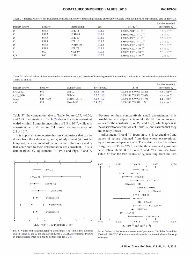
TABLE 27. Inferred values of the Boltzmann constant k in order of increasing standard uncertainty obtained from the indicated experimental data in Table 20.
Primary source Item No. Identification Sec. k=(J K�1)
Relative standard
uncertainty ur
R B58:6 LNE-11 10.1.2 1:380 6477(17)� 10�23 1:2� 10�6
R B58:2 NIST-88 10.1.1 1:380 6503(25)� 10�23 1:8� 10�6
R B58:3 LNE-09 10.1.2 1:380 6495(37)� 10�23 2:7� 10�6
R B58:4 NPL-10 10.1.3 1:380 6496(43)� 10�23 3:1� 10�6
R B58:5 INRIM-10 10.1.4 1:380 640(10)� 10�23 7:5� 10�6
R B58:1 NPL-79 10.1.1 1:380 656(12)� 10�23 8:4� 10�6
k B59 NIST-07 10.2.1 1:380 653(13)� 10�23 9:1� 10�6
k=h B60 NIST-11 10.2.2 1:380 652(17)� 10�23 1:2� 10�5
TABLE 28. Inferred values of the electron relative atomic mass Ar(e) in order of increasing standard uncertainty obtained from the indicated experimental data in
Tables 20 and 22.
Primary source Item No. Identification Sec. and Eq. Ar(e)
Relative standard
uncertainty ur
fs(C)=fc(C) B17 GSI-02 5.3.2 (188) 0.000 548 579 909 32(29) 5:2� 10�10
fs(O)=fc(O) B18 GSI-04 5.3.2 (189) 0.000 548 579 909 57(42) 7:6� 10�10
Δnp�Heþ C16�C30 CERN�06=10 4.2.3 (102) 0.000 548 579 909 14(75) 1:4� 10�9
Ar(e) B11 UWash-95 3.4 (20) 0.000 548 579 9111(12) 2:1� 10�9
CODATA RECOMMENDED VALUES: 2010 043109-59
Table 37, the companion table to Table 36, are 0.75, �0:56,and 2.88. Examination of Table 29 shows that �K is consistent
with 0within 1.2 times its uncertainty of 1:8� 10�8, while �J isconsistent with 0 within 2.4 times its uncertainty of
2:4� 10�8.
It is important to recognize that any conclusions that can be
drawn from the values of �K and �J of adjustment (i) must be
tempered, because not all of the individual values of �K and �Jthat contribute to their determination are consistent. This is
demonstrated by adjustments (ii)–(vii) and Figs. 7 and 8.
FIG. 5. Values of the electron relative atomic mass Ar(e) implied by the input
data in Tables 20 and 22 and the 2006 and 2010 CODATA recommended valuesin chronological order from top to bottom (see Table 28).
Downloaded 31 Dec 2012 to 129.6.13.245. Redistribution subject to AIP lic
[Because of their comparatively small uncertainties, it is
possible in these adjustments to take the 2010 recommended
values for the constants ae, a, R∞, and Ar(e), which appear in
the observational equations of Table 39, and assume that they
are exactly known.]
Adjustments (ii) and (iii) focus on �K: �J is set equal to 0 andvalues of �K are obtained from data whose observational
equations are independent of h. These data are the five values
of RK, items B35:1�B35:5; and the three low-field gyromag-
netic ratios, items B32:1, B32:2, and B33. We see from
Table 29 that the two values of �K resulting from the two
FIG. 6. Values of the Newtonian constant of gravitation G in Table 24 and the2006 and 2010CODATA recommended values in chronological order from topto bottom.
J. Phys. Chem. Ref. Data, Vol. 41, No. 4, 2012
ense or copyright; see http://jpcrd.aip.org/about/rights_and_permissions

TABLE 30. The 28 adjusted constants (variables) used in the least-squares
multivariate analysis of the Rydberg-constant data given in Table 18. Theseadjusted constants appear as arguments of the functions on the right-hand side othe observational equations of Table 31.
Adjusted constant Symbol
Rydberg constant R∞
Bound-state proton rms charge radius rpBound-state deuteron rms charge radius rdAdditive correction to EH(1S1=2)=h dH(1S1=2)
Additive correction to EH(2S1=2)=h dH(2S1=2)
Additive correction to EH(3S1=2)=h dH(3S1=2)
Additive correction to EH(4S1=2)=h dH(4S1=2)
Additive correction to EH(6S1=2)=h dH(6S1=2)
Additive correction to EH(8S1=2)=h dH(8S1=2)
Additive correction to EH(2P1=2)=h dH(2P1=2)
Additive correction to EH(4P1=2)=h dH(4P1=2)
Additive correction to EH(2P3=2)=h dH(2P3=2)
Additive correction to EH(4P3=2)=h dH(4P3=2)
Additive correction to EH(8D3=2)=h dH(8D3=2)
Additive correction to EH(12D3=2)=h dH(12D3=2)
Additive correction to EH(4D5=2)=h dH(4D5=2)
Additive correction to EH(6D5=2)=h dH(6D5=2)
Additive correction to EH(8D5=2)=h dH(8D5=2)
Additive correction to EH(12D5=2)=h dH(12D5=2)
Additive correction to ED(1S1=2)=h dD(1S1=2)
Additive correction to ED(2S1=2)=h dD(2S1=2)
Additive correction to ED(4S1=2)=h dD(4S1=2)
Additive correction to ED(8S1=2)=h dD(8S1=2)
Additive correction to ED(8D3=2)=h dD(8D3=2)
Additive correction to ED(12D3=2)=h dD(12D3=2)
Additive correction to ED(4D5=2)=h dD(4D5=2)
Additive correction to ED(8D5=2)=h dD(8D5=2)
Additive correction to ED(12D5=2)=h dD(12D5=2)
TABLE 29. Summary of the results of several least-squares adjustments to
investigate the relations KJ ¼ (2e=h)(1þ �J) and RK ¼ (h=e2)(1þ �K). See
the text for an explanation and discussion of each adjustment, but in brief,
adjustment (i) uses all the data, (ii) assumes KJ ¼ 2e=h (that is, �J ¼ 0) andobtains �K from the five measured values of RK, (iii) is based on the sameassumption and obtains �K from the two values of the proton gyromagnetic ratioand one value of the helion gyromagnetic ratio, (iv) is (iii) but assumesRK ¼ h=e2 (that is, �K ¼ 0) and obtains �J in place of �K, (v)–(vii) are basedon the same assumption and obtain �J from all the measured values given inTable 20 for the quantities indicated.
Adjustment Data includeda 108�K 108�J
(i) All 2.2(1.8) 5.7(2.4)
(ii) RK 2.9(1.8) 0
(iii) G 0p;h�90(lo) �25.4(9.3) 0
(iv) G 0p;h�90(lo) 0 �25.4(9.3)
(v) G 0p�90(hi), KJ,
K2J RK, F 90
0 23.7(72.0)
(vi) G 0p�90(hi), KJ,
K2J RK, F 90, NA
0 8.6(2.2)
(vii) G 0p�90(hi), ½KJ�,½K2
J RK�, F 90, ½NA�0 8.6(4.4)
aThe data items in brackets have their uncertainties expanded by a factor of 2.
043109-60 MOHR, TAYLOR, AND NEWELL
adjustments not only have opposite signs but their difference is
3:0udiff . Figure 7 compares the combined value of �K obtained
from the five values ofRK with the five individual values, while
Fig. 8 does the same for the results obtained from the three
gyromagnetic ratios.
Adjustments (iv)–(vii) focus on �J: �K is set equal to 0 and
values of �J are, with the exception of adjustment (iv), obtained
from data whose observational equations are dependent on h.
Examination of Table 29 shows that although the values of �Jfrom adjustments (iv) and (v) are of opposite sign, their
difference of 49:1� 10�8 is less than the 73:0� 10�8 uncer-
tainty of the difference. However, the difference between the
values of �J from adjustments (iv) and (vi) is 3:6udiff , and is
3:3udiff even for the value of �J from adjustment (vii), in which
TABLE 31. Observational equations that express the input data related to R∞ in Table 18 as functions of the adjusted constants in Table 30. The numbers in the firscolumn correspond to the numbers in the first column of Table 18. Energy levels of hydrogenic atoms are discussed in Sec. 4.1. As pointed out at the beginning of thasection, EX(nLj)=h is in fact proportional to cR∞ and independent of h, hence h is not an adjusted constant in these equations. See Sec. 13.2 for an explanation of thesymbol ¼: .Type of input datum Observational equation
A1�A16 dH(nLj) ¼: dH(nLj)
A17�A25 dD(nLj) ¼: dD(nLj)
A26�A31, A38, A39 nH(n1L1j1 � n2L2j2 ) ¼: ½EH(n2L2j2 ;R∞;a;Ar(e);Ar(p); rp; dH(n2L2j2 ))
�EH(n1L1j1 ;R∞;a;Ar(e);Ar(p); rp; dH(n1L1j1 ))�=hA32�A37 nH(n1L1j1 � n2L2j2 )� 1
4nH(n3L3j3 � n4L4j4 ) ¼: fEH(n2L2j2 ;R∞;a;Ar(e);Ar(p); rp; dH(n2L2j2 ))
�EH(n1L1j1 ;R∞;a;Ar(e);Ar(p); rp; dH(n1L1j1 ))� 14½EH(n4L4j4 ;R∞;a;Ar(e);Ar(p); rp; dH(n4L4j4 ))
�EH(n3L3j3 ;R∞;a;Ar(e);Ar(p); rp; dH(n3L3j3 ))�g=hA40�A44 nD(n1L1j1 � n2L2j2 ) ¼: ½ED(n2L2j2 ;R∞;a;Ar(e);Ar(d); rd; dD(n2L2j2 ))� ED(n1L1j1 ;R∞;a;Ar(e);Ar(d); rd; dD(n1L1j1 ))�=hA45, A46 nD(n1L1j1 � n2L2j2 )� 1
4nD(n3L3j3 � n4L4j4 ) ¼: fED(n2L2j2 ;R∞;a;Ar(e);Ar(d); rd; dD(n2L2j2 ))
�ED(n1L1j1 ;R∞;a;Ar(e);Ar(d); rd; dD(n1L1j1 ))� 14½ED(n4L4j4 ;R∞;a;Ar(e);Ar(d); rd; dD(n4L4j4 ))
�ED(n3L3j3 ;R∞;a;Ar(e);Ar(d); rd; dD(n3L3j3 ))�g=hA47 nD(1S1=2 � 2S1=2)� nH(1S1=2 � 2S1=2) ¼: fED(2S1=2;R∞;a;Ar(e);Ar(d); rd; dD(2S1=2))
�ED(1S1=2;R∞;a;Ar(e);Ar(d); rd; dD(1S1=2))� ½EH(2S1=2;R∞;a;Ar(e);Ar(p); rp; dH(2S1=2))
�EH(1S1=2;R∞;a;Ar(e);Ar(p); rp; dH(1S1=2))�g=hA48 rp ¼: rpA49 rd ¼: rd
J. Phys. Chem. Ref. Data, Vol. 41, No. 4, 2012
Downloaded 31 Dec 2012 to 129.6.13.245. Redistribution subject to AIP license or copyright; see http://jpcrd.aip.org/about/rights_and_permissions
f
tt

TABLE 32. The 39 adjusted constants (variables) used in the least-squares
multivariate analysis of the input data in Table 20. These adjusted constantsappear as arguments of the functions on the right-hand side of the observationalequations of Table 33.
Adjusted constant Symbol
Electron relative atomic mass Ar(e)
Proton relative atomic mass Ar(p)
Neutron relative atomic mass Ar(n)
Deuteron relative atomic mass Ar(d)
Triton relative atomic mass Ar(t)
Helion relative atomic mass Ar(h)
Alpha particle relative atomic mass Ar(a)16O7þ relative atomic mass Ar(
16O7þ )87Rb relative atomic mass Ar(
87Rb)133Cs relative atomic mass Ar(
133Cs)
Average vibrational excitation energy Ar(Eav)
Fine-structure constant a
Additive correction to ae(th) deMuon magnetic-moment anomaly amAdditive correction to gC(th) dCAdditive correction to gO(th) dOElectron-proton magnetic-moment ratio me�=mp
Deuteron-electron magnetic-moment ratio md=me�
Triton-proton magnetic-moment ratio mt=mp
Shielding difference of d and p in HD sdp
Shielding difference of t and p in HT stp
Electron to shielded proton magnetic-moment ratio me�=m0p
Shielded helion to shielded proton magnetic-moment ratio m0h=m
0p
Neutron to shielded proton magnetic-moment ratio mn=m0p
Electron-muon mass ratio me=mm
Additive correction to ΔnMu(th) dMu
Planck constant h
Molar gas constant R
Copper Ka1 x unit xu(CuKa1)
Molybdenum Ka1 x unit xu(MoKa1)
Angstrom star A �
d220 of Si crystal ILL d220(ILL)
d220 of Si crystal N d220(N)
d220 of Si crystal WASO 17 d220(W17)
d220 of Si crystal WASO 04 d220(W04)
d220 of Si crystal WASO 4.2a d220(W4:2a)
d220 of Si crystal MO� d220(MO�)d220 of Si crystal NR3 d220(NR3)
d220 of Si crystal NR4 d220(NR4)
d220 of an ideal Si crystal d220
CODATA RECOMMENDED VALUES: 2010 043109-61
the uncertainties of themost accurate data have been increased
by the factor 2. (The multiplicative factor 2 is that used in
adjustment 2 and the final adjustment; see Tables 36 and 37,
and their associated text.) On the other hand, we see that the
value of �J from adjustment (vi) is consistent with 0 only to
within 3.9 times its uncertainty, but that this is reduced to 2.0
for the value of �J from adjustment (vii) which uses expanded
uncertainties.
The results of the adjustments discussed above reflect the
disagreement of the NIST-07 watt-balance value for K2J RK,
and to a lesser extent that of the similar NIST-98 value, items
B37:3 and B37:2, with the IAC-11 enriched silicon value of
NA, item B54; and the disagreement of the NIST-89 result for
Downloaded 31 Dec 2012 to 129.6.13.245. Redistribution subject to AIP lic
G 0p�90(lo), and to a lesser extent the KR/VN-98 result for
G 0h�90(lo), items B32:1 and B33, with the highly accurate
values of a. If adjustment (i) is repeated with these five data
deleted,we find �K ¼ 2:8(1:8)� 10�8 and �J ¼ 15(49)�10�8.
These values can be interpreted as confirming that �K is
consistent with 0 to within 1.6 times its uncertainty of
1:8� 10�8 and that �J is consistent with 0 well within its
uncertainty of 49� 10�8.
We conclude this section by briefly discussing recent efforts
to close themetrology triangle.Although there are variants, the
basic idea is to use a single electron tunneling (SET) device
that generates a quantized current I ¼ ef when an alternating
voltage of frequency f is applied to it, where as usual e is the
elementary charge. The current I is then compared to a current
derived from Josephson and quantum-Hall-effect devices. In
view of quantization of charge in units of e and conservation of
charge, the equality of the currents shows that KJRKe ¼ 2, as
expected, within the uncertainty of the measurements (Keller,
2008; Keller et al., 2008; Feltin and Piquemal, 2009).
Although there is no indication from the results reported to
date that this relation is not valid, the uncertainties of the
results are at best at the 1 to 2 parts in 106 level (Keller,
Zimmerman, and Eichenberger, 2007; Keller et al., 2008;
Feltin et al., 2011; Camarota et al., 2012).
14. The 2010 CODATA RecommendedValues
14.1. Calculational details
The 168 input data and their correlation coefficients initially
considered for inclusion in the 2010 CODATA adjustment of
the values of the constants are given in Tables 18–23. The 2010
recommended values are based on adjustment 3, called the
final adjustment, summarized in Tables 36–38 and discussed
in the associated text. Adjustment 3 omits 20 of the 168
initially considered input data, namely, items B10:1, B10:2,B13:1,B32:1�B36:2,B37:5,B38,B56,B59, andB60, becauseof their low weight (self-sensitivity coefficient Sc < 0:01).
However, because the observational equation for h=m(133Cs),
item B56, depends on Ar(133Cs) but item B56 is deleted
because of its low weight, the two values of Ar(133Cs), items
B10:1 and B10:2, are also deleted and Ar(133Cs) itself is
deleted as an adjusted constant. Further, the initial uncertain-
ties of five input data, items B37:1�B37:4 and B54, are
multiplied by the factor 2, with the result that the absolute
values of the normalized residuals jrij of the five data are lessthan 1.4 and their disagreement is reduced to an acceptable
level.
Each input datum in this final adjustment has a self-sensi-
tivity coefficient Sc greater than 0.01, or is a subset of the data
of an experiment or series of experiments that provide an input
datum or input data with Sc > 0:01. Not counting such input
data with Sc < 0:01, the seven data with jrij > 1:2 are A50,
J. Phys. Chem. Ref. Data, Vol. 41, No. 4, 2012
ense or copyright; see http://jpcrd.aip.org/about/rights_and_permissions

TABLE 33. Observational equations that express the input data in Table 20 as functions of the adjusted constants in Table 32. The numbers in the firstcolumn correspond to the numbers in the first column of Table 20. For simplicity, the lengthier functions are not explicitly given. See Sec. 13.2 for an explanation ofthe symbol ¼: .Type of input datum Observational equation Sec.
B1 Ar(1H) ¼: Ar(p)þ Ar(e)� Eb(
1H)=muc2 3.2
B2 Ar(2H) ¼: Ar(d)þ Ar(e)� Eb(
2H)=muc2 3.2
B3 Ar(Eav) ¼: Ar(Eav) 3.3
B4fc(H
þ�2 )
fc(d)¼: Ar(d)
2Ar(p)þ Ar(e)� ½2EI(H)þ EB(H2)� EI(H2)� Eav�=muc23.3
B5fc(t)
fc(Hþ�2 )
¼: 2Ar(p)þ Ar(e)� ½2EI(H)þ EB(H2)� EI(H2)� Eav�=muc2
Ar(t)
3.3
B6fc(
3Heþ )fc(H
þ�2 )
¼: 2Ar(p)þ Ar(e)� ½2EI(H)þ EB(H2)� EI(H2)� Eav�=muc2
Ar(h)þ Ar(e)� EI(3Heþ )=muc2
3.3
B7 Ar(4He) ¼: Ar(a)þ 2Ar(e)� Eb(
4He)=muc2 3.2
B8 Ar(16O) ¼: Ar(
16O7þ )þ 7Ar(e)� ½Eb(16O)� Eb(
16O7þ )�=muc2 3.2
B9 Ar(87Rb) ¼: Ar(
87Rb)
B10 Ar(133Cs) ¼: Ar(
133Cs)
B11 Ar(e) ¼: Ar(e)
B12 de ¼: de
B13 ae ¼: ae(a; de) 5.1.1
B14 R ¼: � am
1þ ae(a; de)
me
mm
me�
mp
5.2.2
B15 dC ¼: dC
B16 dO ¼: dO
B17fs(
12C5þ )fc(
12C5þ )¼: � gC(a; dC)
10Ar(e)12� 5Ar(e)þ Eb(
12C)� Eb(12C5þ )
muc2
� �5.3.2
B18fs(
16O7þ )fc(
16O7þ )¼: � gO(a; dO)
14Ar(e)Ar(
16O7þ )5.3.2
B19 me� (H)
mp(H)¼: ge� (H)
ge�
gp(H)
gp
� ��1me�
mp
B20 md(D)
me� (D)¼: gd(D)
gd
ge� (D)
ge�
� ��1md
me�
B21mp(HD)
md(HD)¼: ½1þ sdp�
mp
me�
me�
md
B22 sdp ¼: sdp
B23mt(HT)
mp(HT)¼: ½1� stp� mt
mp
B24 stp ¼: stp
B25me� (H)
m0p
¼: ge� (H)
ge�
me�
m0p
B26m0h
m0p
¼: m0h
m0p
B27mn
m0p
¼: mn
m0p
B28 dMu ¼: dMu
B29 ΔnMu ¼: ΔnMu R∞;a;me
mm; dMu
� �6.2.1
B30; B31 n(fp) ¼: n fp;R∞;a;me
mm;me�
mp
; de; dMu
� �6.2.2
B32G 0
p�90(lo) ¼: � KJ�90RK�90½1þ ae(a; de)�a3
2m0R∞
me�
m0p
!�1
J. Phys. Chem. Ref. Data, Vol. 41, No. 4, 2012
043109-62 MOHR, TAYLOR, AND NEWELL
Downloaded 31 Dec 2012 to 129.6.13.245. Redistribution subject to AIP license or copyright; see http://jpcrd.aip.org/about/rights_and_permissions

TABLE 33. Observational equations that express the input data in Table 20 as functions of the adjusted constants in Table 32. The numbers in the firstcolumn correspond to the numbers in the first column of Table 20. For simplicity, the lengthier functions are not explicitly given. See Sec. 13.2 for an explanation ofthe symbol ¼: .—Continued
Type of input datum Observational equation Sec.
B33 G 0h�90(lo) ¼:
KJ�90RK�90½1þ ae(a; de)�a3
2m0R∞
me�
m0p
!�1m0h
m0p
B34 G 0p�90(hi) ¼: � c½1þ ae(a; de)�a2
KJ�90RK�90R∞h
me�
m0p
!�1
B35 RK ¼: m0c
2a
B36 KJ ¼: 8a
m0ch
� �1=2
B37 K2J RK ¼: 4
h
B38 F 90 ¼: cMuAr(e)a2
KJ�90RK�90R∞h
B39�B41 d220(X) ¼: d220(X)
B42�B53d220(X)
d220(Y)� 1 ¼: d220(X)
d220(Y)� 1
B54 NA ¼: cMuAr(e)a2
2R∞h
B55λmeas
d220(ILL)¼: a2Ar(e)
R∞d220(ILL)
Ar(n)þ Ar(p)
½Ar(n)þ Ar(p)�2 � A2r (d)
9.3
B56; B57h
m(X)¼: Ar(e)
Ar(X)
ca2
2R∞
7.1
B58 R ¼: R
B59 k ¼: 2R∞hR
cMuAr(e)a2
B60k
h¼: 2R∞R
cMuAr(e)a2
B61; B64λ(CuKa1)
d220(X)¼: 1 537:400 xu(CuKa1)
d220(X)
9.4
B62 λ(WKa1)
d220(N)¼: 0:209 010 0 A
�
d220(N)
9.4
B63λ(MoKa1)
d220(N)¼: 707:831 xu(MoKa1)
d220(N)
9.4
CODATA RECOMMENDED VALUES: 2010 043109-63
B11, B37:3, B54, C19, C21, and C28; their values of ri are
�1:24, 1.43, 1.39, �1:31, �1:60, �1:83, and 1.76,
respectively.
Asdiscussed inSec. 13.2.1, the2010 recommendedvalueofG
is the weightedmean of the 11measured values in Table 24 after
the uncertainty of each is multiplied by the factor 14. Although
these data can be treated separately because they are independent
Downloaded 31 Dec 2012 to 129.6.13.245. Redistribution subject to AIP lic
of all of the other data, they could have been included with the
other data. For example, if the 11 values of G with expanded
uncertainties are added to the 148 input data of adjustment 3,G is
taken as an additional adjusted constant so that these 11 values
can be included in a new adjustment using the observational
equation G ¼: G, and the so-modified adjustment 3 is repeated,
then we find for this “grand final adjustment” that N ¼ 160,
J. Phys. Chem. Ref. Data, Vol. 41, No. 4, 2012
ense or copyright; see http://jpcrd.aip.org/about/rights_and_permissions

TABLE 34. The 15 adjusted constants relevant to the antiprotonic helium data
given in Table 22. These adjusted constants appear as arguments of thetheoretical expressions on the right-hand side of the observational equationsof Table 35.
Transition Adjusted constant
p4Heþ : (32; 31)→ (31; 30) dp�4Heþ(32; 31 : 31; 30)
p4Heþ : (35; 33)→ (34; 32) dp�4Heþ(35; 33 : 34; 32)
p4Heþ : (36; 34)→ (35; 33) dp�4Heþ(36; 34 : 35; 33)
p4Heþ : (37; 34)→ (36; 33) dp�4Heþ(37; 34 : 36; 33)
p4Heþ : (39; 35)→ (38; 34) dp�4Heþ(39; 35 : 38; 34)
p4Heþ : (40; 35)→ (39; 34) dp�4Heþ(40; 35 : 39; 34)
p4Heþ : (37; 35)→ (38; 34) dp�4Heþ(37; 35 : 38; 34)
p4Heþ : (33; 32)→ (31; 30) dp�4Heþ(33; 32 : 31; 30)
p4Heþ : (36; 34)→ (34; 32) dp�4Heþ(36; 34 : 34; 32)
p3Heþ : (32; 31)→ (31; 30) dp�3Heþ(32; 31 : 31; 30)
p3Heþ : (34; 32)→ (33; 31) dp�3Heþ(34; 32 : 33; 31)
p3Heþ : (36; 33)→ (35; 32) dp�3Heþ(36; 33 : 35; 32)
p3Heþ : (38; 34)→ (37; 33) dp�3Heþ(38; 34 : 37; 33)
p3Heþ : (36; 34)→ (37; 33) dp�3Heþ(36; 34 : 37; 33)
p3Heþ : (35; 33)→ (33; 31) dp�3Heþ(35; 33 : 33; 31)
043109-64 MOHR, TAYLOR, AND NEWELL
M ¼ 83, n ¼ 77, x2 ¼ 59:1, p(59:1j77) ¼ 0:94, and
RB ¼ 0:88. Of course, the resulting values of the adjusted
constants, and of the normalized residuals and self-sensitivity
coefficients of the input data, are exactly the same as those from
adjustment 3 and the weighted mean of the 11 measured values
of G with expanded uncertainties.
In any event, the 2010 recommended values are calculated
from the set of best estimated values, in the least-squares sense,
of 82 adjusted constants, including G, and their variances and
covariances, together with (i) those constants that have exact
values such as m0 and c; and (ii) the values of mτ, GF, and
TABLE 35. Observational equations that express the input data related to antiprotoni
numbers in the first column correspond to the numbers in the first column of Tableare given in Sec. 4.2. See Sec. 13.2 for an explanation of the symbol ¼: .Type of input datum Observational equation
C1�C9 dp4Heþ (n; l : n0; l0) ¼: dp4Heþ (n; l : n
0; l0)
C10�C15 dp3Heþ (n; l : n0; l0) ¼: dp3Heþ (n; l : n
0; l0)
C16�C24 Δnp4Heþ (n; l : n0; l0) ¼: Δn(0)
p4Heþ (n; l : n0; l0)þ ap4
þbp4Heþ (n; l : n0; l0)
Ar(e)
Ar(a)
� �(0)Ar(a)
Ar(e)
� �� 1
" #
C25�C30 Δnp3Heþ (n; l : n0; l0) ¼: Δn (0)
p3Heþ (n; l : n0; l0)þ ap3
þbp3Heþ (n; l : n0; l0)
Ar(e)
Ar(h)
� �(0)Ar(h)
Ar(e)
� �� 1
" #
J. Phys. Chem. Ref. Data, Vol. 41, No. 4, 2012
Downloaded 31 Dec 2012 to 129.6.13.245. Redistribution subject to AIP lic
sin2uW given in Sec. 12 of this report; see Sec. V.B of
CODATA-98 for details.
14.2. Tables of values
Tables 40–47 give the 2010 CODATA recommended
values of the basic constants and conversion factors of physics
and chemistry and related quantities. Although very similar in
form and content to their 2006 counterparts, several new
recommended values have been included in the 2010 tables
and a few have been deleted. The values of the four new
constants,mn � mp in kg and u, and (mn � mp)c2 in J andMeV,
are given in Table 41 under the heading “Neutron, n”; and the
values of the four new constants mh, mh=mB, mh=mN, and ghare given in the same table under the heading “Helion, h.” The
three constants deleted, mt=me, mt=mp, and mt=mn, were in
the 2006 version of Table 41 under the heading “Triton, t.” It
was decided that these constants were of limited interest
and the values can be calculated from other constants in the
table.
The values of the four new helion-related constants are
calculated from the adjusted constant m0h=m
0p and the theore-
tically predicted shielding correction sh ¼ 59:967 43(10)
�10�6 due to Rudzi�nski, Puchalski, and Pachucki (2009)
using the relation m0h ¼ mh(1� sh); see Sec. 6.1.2.
Table 40 is a highly abbreviated list of the values of the
constants and conversion factors most commonly used.
Table 41 is a much more extensive list of values categorized
as follows: UNIVERSAL; ELECTROMAGNETIC;
ATOMIC AND NUCLEAR; and PHYSICOCHEMICAL.
The ATOMIC AND NUCLEAR category is subdivided into
11 subcategories: General; Electroweak; Electron, e�; Muon,
m�; Tau, τ�; Proton, p; Neutron, n; Deuteron, d; Triton, t;Helion, h; and Alpha particle, a. Table 42 gives the variances,covariances, and correlation coefficients of a selected group
of constants. (Use of the covariance matrix is discussed
in Appendix E of CODATA-98.) Table 43 gives the
c helium in Table 22 as functions of adjusted constants in Tables 32 and 34. The22. Definitions of the symbols and values of the parameters in these equations
Heþ (n; l : n0; l0)
Ar(e)
Ar(p)
� �(0)Ar(p)
Ar(e)
� �� 1
" #
þ dp4Heþ (n; l : n0; l0)
Heþ (n; l : n0; l0)
Ar(e)
Ar(p)
� �(0)Ar(p)
Ar(e)
� �� 1
" #
þ dp3Heþ (n; l : n0; l0)
ense or copyright; see http://jpcrd.aip.org/about/rights_and_permissions

TABLE 36. Summary of the results of some of the least-squares adjustments used to analyze the input data given in Tables 18–23. The values of a and h are those
obtained in the adjustment,N is the number of input data,M is the number of adjusted constants, n ¼ N �M is the degrees of freedom, andRB ¼ ffiffiffiffiffiffiffiffiffiffix2=n
pis the Birge
ratio. See the text for an explanation and discussion of each adjustment, but in brief, adjustment 1 is all the data; 2 is the same as 1 except with the uncertainties of thekey data that determine hmultiplied by 2; 3 is 2 with the low-weight input data deleted and is the adjustment on which the 2010 recommended values are based; 4 is 2with the input data that provide themost accurate values of alpha deleted; and 5 is 1with the input data that provide themost accurate values of h deleted aswell as low-weight data for a.
Adj. N M n x2 RB a�1 ur(a�1) h=(J s) ur(h)
1 169 83 86 89.3 1.02 137.035 999 075(44) 3:2� 10�10 6:626 069 58(15)� 10�34 2:2� 10�8
2 169 83 86 75.7 0.94 137.035 999 073(44) 3:2� 10�10 6:626 069 57(29)� 10�34 4:4� 10�8
3 149 82 67 58.1 0.93 137.035 999 074(44) 3:2� 10�10 6:626 069 57(29)� 10�34 4:4� 10�8
4 161 81 80 69.4 0.93 137.036 0005(20) 1:4� 10�8 6:626 069 50(31)� 10�34 4:7� 10�8
5 154 82 72 57.2 0.89 137.035 999 074(44) 3:2� 10�10 6:626 069 48(80)� 10�34 1:2� 10�7
TABLE 37. Normalized residuals ri and self-sensitivity coefficients Sc that result from the five least-squares adjustments summarized in Table 36 for the three inputdata with the largest absolute values of ri in adjustment 1. Sc is a measure of how the least-squares estimated value of a given type of input datum depends on aparticularmeasured or calculated value of that type of datum; seeAppendixE ofCODATA-98. See the text for an explanation and discussion of each adjustment; briefexplanations are given in the caption to Table 36.
Adj. 1 Adj. 2 Adj. 3 Adj. 4 Adj. 5
Item No. Input quantity Identification ri Sc ri Sc ri Sc ri Sc ri Sc
B37:3 K2J RK NIST-07 2.83 0.367 1.39 0.367 1.39 0.371 1.23 0.413 Deleted
B54 NA IAC-11 �2.57 0.555 �1.32 0.539 �1.31 0.546 �1.16 0.587 Deleted
B32:1 G 0p�90(lo) NIST-89 2.19 0.010 2.19 0.010 Deleted 2.46 0.158 Deleted
TABLE 38. Summaryof the results of someof the least-squares adjustments used to analyze the input data related toR∞. The values ofR∞, rp, and rd are those obtained
in the indicated adjustment, N is the number of input data,M is the number of adjusted constants, n ¼ N �M is the degrees of freedom, and RB ¼ ffiffiffiffiffiffiffiffiffiffix2=n
pis the
Birge ratio. See the text for an explanation and discussion of each adjustment. In brief, adjustment 6 is 3 but the scattering data for the nuclear radii are omitted; 7 is 3,but with only the hydrogen data included (no isotope shift); 8 is 7 with the rp data deleted; 9 and 10 are similar to 7 and 8, but for the deuterium data; 11 is 3 with themuonic Lamb-shift value of rp included; and 12 is 11, but without the scattering values of rp and rd.
Adj. N M n x2 RB R∞ (m�1) ur(R∞) rp (fm) rd (fm)
3 149 82 67 58.1 0.93 10 973 731.568 539(55) 5:0� 10�12 0.8775(51) 2.1424(21)
6 146 82 64 55.5 0.93 10 973 731.568 521(82) 7:4� 10�12 0.8758(77) 2.1417(31)
7 131 72 59 53.4 0.95 10 973 731.568 561(60) 5:5� 10�12 0.8796(56)
8 129 72 57 52.5 0.96 10 973 731.568 528(94) 8:6� 10�12 0.8764(89)
9 114 65 49 46.9 0.98 10 973 731.568 37(13) 1:1� 10�11 2.1288(93)
10 113 65 48 46.8 0.99 10 973 731.568 28(30) 2:7� 10�11 2.121(25)
11 150 82 68 104.9 1.24 10 973 731.568 175(12) 1:1� 10�12 0.842 25(65) 2.128 24(28)
12 147 82 65 74.3 1.07 10 973 731.568 171(12) 1:1� 10�12 0.841 93(66) 2.128 11(28)
J. Phys. Chem. Ref. Data, Vol. 41, No. 4, 2012
CODATA RECOMMENDED VALUES: 2010 043109-65
Downloaded 31 Dec 2012 to 129.6.13.245. Redistribution subject to AIP license or copyright; see http://jpcrd.aip.org/about/rights_and_permissions

TABLE 39. Generalized observational equations that express input data
B32�B38 in Table 20 as functions of the adjusted constants in Tables 30 and32 with the additional adjusted constants �J and �K as given in Eqs. (285) and(286). The numbers in the first column correspond to the numbers in the firstcolumn of Table 20. For simplicity, the lengthier functions are not explicitlygiven. See Sec. 13.2 for an explanation of the symbol ¼: .
Type of
input datum Generalized observational equation
B32� G 0p�90(lo) ¼: � KJ�90RK�90½1þ ae(a; de)�a3
2m0R∞(1þ �J)(1þ �K)
me�
m0p
!�1
B33� G 0h�90(lo) ¼:
KJ�90RK�90½1þ ae(a; de)�a3
2m0R∞(1þ �J)(1þ �K)
me�
m0p
!�1m0h
m0p
B34� G 0p�90(hi) ¼: � c½1þ ae(a; de)�a2
KJ�90RK�90R∞h(1þ �J)(1þ �K)
me�
m0p
!�1
B35� RK ¼: m0c
2a(1þ �K)
B36� KJ ¼: 8a
m0ch
� �1=2
(1þ �J)
B37� K2J RK ¼: 4
h(1þ �J)
2(1þ �K)
B38� F 90 ¼: cMuAr(e)a2
KJ�90RK�90R∞h(1þ �J)(1þ �K)
FIG. 7. Comparison of the five individual values of �K obtained from the five
values of RK, data items B35:1�B35:5, and the combined value (open circle)
fromadjustment (ii) given in Table 29. The applicable observational equation inTable 39 is B35�.
FIG. 8. Comparison of the three individual values of �K obtained from the three
low-field gyromagnetic ratios, data items B32:1, B32:2, and B33, and the
combined value (open circle) from adjustment (iii) given in Table 29. Theapplicable observational equations in Table 39 are B32� and B33�. Because othe form of these equations, the value of �K when �J ¼ 0 is identical to the valueof �J when �K ¼ 0, hence the label at the bottom of the figure.
J. Phys. Chem. Ref. Data, Vol. 41, No. 4, 2012
043109-66 MOHR, TAYLOR, AND NEWELL
Downloaded 31 Dec 2012 to 129.6.13.245. Redistribution subject to AIP license or copyright; see http://jpcrd.aip.org/about/rights_and_permissions
f
internationally adopted values of various quantities; Table 44
lists the values of a number of x-ray related quantities; Table 45
lists the values of various non-SI units; and Tables 46 and 47
give the values of various energy equivalents.
All of the values given in Tables 40–47 are available on the
Web pages of the Fundamental Constants Data Center of the
NIST Physical Measurement Laboratory at physics.nist.gov/
constants. This electronic version of the 2010 CODATA
recommended values of the constants also includes a
much more extensive correlation coefficient matrix. In fact,
the correlation coefficient of any two constants listed in the
tables is accessible on the Web site, as well as the automatic
conversion of the value of an energy-related quantity
expressed in one unit to the corresponding value expressed
in another unit (in essence, an automated version of Tables 46
and 47).
15. Summary and Conclusion
The focus of this section is (i) comparison of the 2010 and
2006 recommended values of the constants and identification
of those new results that have contributed most to the changes
in the 2006 values; (ii) presentation of several conclusions that
can be drawn from the 2010 recommended values and the input
data on which they are based; and (iii) identification of new
experimental and theoretical work that can advance our
knowledge of the values of the constants.
Topic (iii) is of special importance in light of the adoption by
the 24th General Conference on Weights and Measures

TABLE 40. An abbreviated list of the CODATA recommended values of the fundamental constants of physics and chemistry based on the 2010 adjustment.
Quantity Symbol Numerical value Unit Relative std. uncert. ur
Speed of light in vacuum c, c0 299 792 458 m s�1 Exact
Magnetic constant m0 4π� 10�7 NA�2
¼ 12:566 370 614…� 10�7 NA�2 Exact
Electric constant 1=m0c2 �0 8:854 187 817…� 10�12 Fm�1 Exact
Newtonian constant of gravitation G 6:673 84(80)� 10�11 m3 kg�1 s�2 1:2� 10�4
Planck constant h 6:626 069 57(29)� 10�34 J s 4:4� 10�8
h=2π --h 1:054 571 726(47)� 10�34 J s 4:4� 10�8
Elementary charge e 1:602 176 565(35)� 10�19 C 2:2� 10�8
Magnetic flux quantum h=2e F0 2:067 833 758(46)� 10�15 Wb 2:2� 10�8
Conductance quantum 2e2=h G0 7:748 091 7346(25)� 10�5 S 3:2� 10�10
Electron mass me 9:109 382 91(40)� 10�31 kg 4:4� 10�8
Proton mass mp 1:672 621 777(74)� 10�27 kg 4:4� 10�8
Proton-electron mass ratio mp=me 1836.152 672 45(75) 4:1� 10�10
Fine-structure constant e2=4π�0 --hc a 7:297 352 5698(24)� 10�3 3:2� 10�10
inverse fine-structure constant a�1 137.035 999 074(44) 3:2� 10�10
Rydberg constant a2mec=2h R∞ 10 973 731.568 539(55) m�1 5:0� 10�12
Avogadro constant NA; L 6:022 141 29(27)� 1023 mol�1 4:4� 10�8
Faraday constant NAe F 96 485.3365(21) Cmol�1 2:2� 10�8
Molar gas constant R 8.314 4621(75) Jmol�1 K�1 9:1� 10�7
Boltzmann constant R=NA k 1:380 6488(13)� 10�23 J K�1 9:1� 10�7
Stefan-Boltzmann constant
(π2=60)k4=--h3c2 s 5:670 373(21)� 10�8 Wm�2 K�4 3:6� 10�6
Non-SI units accepted for use with the SI
Electron volt (e=C) J eV 1:602 176 565(35)� 10�19 J 2:2� 10�8
(Unified) atomic mass unit 112m(12C) u 1:660 538 921(73)� 10�27 kg 4:4� 10�8
CODATA RECOMMENDED VALUES: 2010 043109-67
(CGPM) at itsmeeting in Paris inOctober 2011 ofResolution 1
entitled “On the possible future revision of the International
System of Units, the SI,” available on the BIPM Web site at
bipm.org/utils/common/pdf/24_CGPM_Resolutions.pdf.
In brief, this resolution notes the intention of the CIPM to
propose, possibly to the 25th CGPM in 2014, a revision of the
SI. The “newSI,” as it is called to distinguish it from the current
SI, will be the system of units in which seven reference
constants, including the Planck constant h, elementary charge
e, Boltzmann constant k, and Avogadro constant NA, have
exact assigned values. Resolution 1 also looks to CODATA to
provide the necessary values of these four constants for the
new definition. Details of the proposed new SImay be found in
Mills et al. (2011) and the references cited therein; see also
Mohr and Newell (2010) and Taylor (2011).
15.1. Comparison of 2010 and 2006 CODATArecommended values
Table 48 compares the 2010 and 2006 recommended values
of a representative group of constants. The fact that the values
of many constants are obtained from expressions proportional
to the fine-structure constant a, Planck constant h, or molar gas
constant R raised to various powers leads to the regularities
observed in the numbers in columns 2 to 4. For example, the
Downloaded 31 Dec 2012 to 129.6.13.245. Redistribution subject to AIP lic
first six quantities are obtained from expressions proportional
to aa, where jaj ¼ 1, 2, 3, or 6. The next 15 quantities, h
through the magnetic moment of the proton mp, are calculated
from expressions containing the factor ha, where jaj ¼ 1 or
1=2. And the five quantities R through the Stefan-Boltzmann
constant s are proportional to Ra, where jaj ¼ 1 or 4.
Further comments on some of the entries in Table 48 are as
follows.
(i) The large shift in the 2006 recommended value of a is
mainly due to the discovery and correction of an error in the
numerically calculated value of the eighth-order coefficient
A(8)1 in the theoretical expression for ae; see Sec. 5.1.1. Its
reduction in uncertainty is due to two new results. The first is
the 2008 improved value of ae obtained at Harvard University
with a relative standard uncertainty of 2:4� 10�10 compared
to the 6:6� 10�10 uncertainty of the earlier Harvard result
used in the 2006 adjustment. The second result is the 2011
improved LKB atom-recoil value of h=m(87Rb) with an
uncertainty of 1:2� 10�9 compared to the 1:3� 10�8 uncer-
tainty of the earlier LKB result used in 2006. The much
reduced uncertainty of ge is also due to the improved value
of a.
(ii) The change in the 2006 recommended value of h is due to
the 2011 IAC result forNA with a relative standard uncertainty
J. Phys. Chem. Ref. Data, Vol. 41, No. 4, 2012
ense or copyright; see http://jpcrd.aip.org/about/rights_and_permissions

TABLE 41. The CODATA recommended values of the fundamental constants of physics and chemistry based on the 2010 adjustment.
Quantity Symbol Numerical value Unit
Relative std.
uncert. ur
UNIVERSAL
Speed of light in vacuum c, c0 299 792 458 m s�1 Exact
Magnetic constant m0 4p� 10�7 N A�2
¼ 12:566 370 614…� 10�7 N A�2 Exact
Electric constant 1=m0c2 �0 8:854 187 817…� 10�12 F m�1 Exact
Characteristic impedance of vacuum m0c Z0 376.730 313 461… Ω Exact
Newtonian constant of gravitation G 6:673 84(80)� 10�11 m3 kg�1 s�2 1:2� 10�4
G=--hc 6:708 37(80)� 10�39 (GeV=c2)�2 1:2� 10�4
Planck constant h 6:626 069 57(29)� 10�34 J s 4:4� 10�8
4:135 667 516(91)� 10�15 eV s 2:2� 10�8
h=2p --h 1:054 571 726(47)� 10�34 J s 4:4� 10�8
6:582 119 28(15)� 10�16 eV s 2:2� 10�8
--hc 197.326 9718(44) MeV fm 2:2� 10�8
Planck mass (--hc=G)1=2 mP 2:176 51(13)� 10�8 kg 6:0� 10�5
energy equivalent mPc2 1:220 932(73)� 1019 GeV 6:0� 10�5
Planck temperature (--hc5=G)1=2=k TP 1:416 833(85)� 1032 K 6:0� 10�5
Planck length --h=mPc ¼ (--hG=c3)1=2 lP 1:616 199(97)� 10�35 m 6:0� 10�5
Planck time lP=c ¼ (--hG=c5)1=2 tP 5:391 06(32)� 10�44 s 6:0� 10�5
ELECTROMAGNETIC
Elementary charge e 1:602 176 565(35)� 10�19 C 2:2� 10�8
e=h 2:417 989 348(53)� 1014 A J�1 2:2� 10�8
Magnetic flux quantum h=2e F0 2:067 833 758(46)� 10�15 Wb 2:2� 10�8
Conductance quantum 2e2=h G0 7:748 091 7346(25)� 10�5 S 3:2� 10�10
inverse of conductance quantum G�10
12 906.403 7217(42) Ω 3:2� 10�10
Josephson constanta 2e=h KJ 483 597:870(11)� 109 Hz V�1 2:2� 10�8
von Klitzing constantb h=e2 ¼ m0c=2a RK 25 812.807 4434(84) Ω 3:2� 10�10
Bohr magneton e--h=2me mB 927:400 968(20)� 10�26 J T�1 2:2� 10�8
5:788 381 8066(38)� 10�5 eV T�1 6:5� 10�10
mB=h 13:996 245 55(31)� 109 Hz T�1 2:2� 10�8
mB=hc 46.686 4498(10) m�1 T�1 2:2� 10�8
mB=k 0.671 713 88(61) K T�1 9:1� 10�7
Nuclear magneton e--h=2mp mN 5:050 783 53(11)� 10�27 J T�1 2:2� 10�8
3:152 451 2605(22)� 10�8 eV T�1 7:1� 10�10
mN=h 7.622 593 57(17) MHz T�1 2:2� 10�8
mN=hc 2:542 623 527(56)� 10�2 m�1 T�1 2:2� 10�8
mN=k 3:658 2682(33)� 10�4 K T�1 9:1� 10�7
ATOMIC AND NUCLEAR
General
Fine-structure constant e2=4p�0 --hc a 7:297 352 5698(24)� 10�3 3:2� 10�10
inverse fine-structure constant a�1 137.035 999 074(44) 3:2� 10�10
Rydberg constant a2mec=2h R∞ 10 973 731.568 539(55) m�1 5:0� 10�12
R∞c 3:289 841 960 364(17)� 1015 Hz 5:0� 10�12
R∞hc 2:179 872 171(96)� 10�18 J 4:4� 10�8
13.605 692 53(30) eV 2:2� 10�8
Bohr radius a=4pR∞ ¼ 4p�0 --h2=mee
2 a0 0:529 177 210 92(17)� 10�10 m 3:2� 10�10
Hartree energy e2=4p�0a0 ¼ 2R∞hc ¼ a2mec2 Eh 4:359 744 34(19)� 10�18 J 4:4� 10�8
27.211 385 05(60) eV 2:2� 10�8
Quantum of circulation h=2me 3:636 947 5520(24)� 10�4 m2 s�1 6:5� 10�10
h=me 7:273 895 1040(47)� 10�4 m2 s�1 6:5� 10�10
Electroweak
Fermi coupling constantc GF=(--hc)3 1:166 364(5)� 10�5 GeV�2 4:3� 10�6
Weak mixing angled uW (on-shell scheme)
sin2uW ¼ s2W ≡ 1� (mW=mZ)2 sin2uW 0.2223(21) 9:5� 10�3
Electron, e�
Electron mass me 9:109 382 91(40)� 10�31 kg 4:4� 10�8
5:485 799 0946(22)� 10�4 u 4:0� 10�10
energy equivalent mec2 8:187 105 06(36)� 10�14 J 4:4� 10�8
0.510 998 928(11) MeV 2:2� 10�8
J. Phys. Chem. Ref. Data, Vol. 41, No. 4, 2012
043109-68 MOHR, TAYLOR, AND NEWELL
Downloaded 31 Dec 2012 to 129.6.13.245. Redistribution subject to AIP license or copyright; see http://jpcrd.aip.org/about/rights_and_permissions

TABLE 41. The CODATA recommended values of the fundamental constants of physics and chemistry based on the 2010 adjustment.—Continued
Quantity Symbol Numerical value Unit
Relative std.
uncert. ur
Electron-muon mass ratio me=mm 4:836 331 66(12)� 10�3 2:5� 10�8
Electron-tau mass ratio me=mt 2:875 92(26)� 10�4 9:0� 10�5
Electron-proton mass ratio me=mp 5:446 170 2178(22)� 10�4 4:1� 10�10
Electron-neutron mass ratio me=mn 5:438 673 4461(32)� 10�4 5:8� 10�10
Electron-deuteron mass ratio me=md 2:724 437 1095(11)� 10�4 4:0� 10�10
Electron-triton mass ratio me=mt 1:819 200 0653(17)� 10�4 9:1� 10�10
Electron-helion mass ratio me=mh 1:819 543 0761(17)� 10�4 9:2� 10�10
Electron to alpha particle mass ratio me=ma 1:370 933 555 78(55)� 10�4 4:0� 10�10
Electron charge-to-mass quotient �e=me �1:758 820 088(39)� 1011 C kg�1 2:2� 10�8
Electron molar mass NAme M(e), Me 5:485 799 0946(22)� 10�7 kg mol�1 4:0� 10�10
Compton wavelength h=mec λC 2:426 310 2389(16)� 10�12 m 6:5� 10�10
λC=2p ¼ a a0 ¼ a2=4pR∞ λC 386:159 268 00(25)� 10�15 m 6:5� 10�10
Classical electron radius a2a0 re 2:817 940 3267(27)� 10�15 m 9:7� 10�10
Thomson cross section (8p=3)r2e se 0:665 245 8734(13)� 10�28 m2 1:9� 10�9
Electron magnetic moment me �928:476 430(21)� 10�26 J T�1 2:2� 10�8
to Bohr magneton ratio me=mB �1:001 159 652 180 76(27) 2:6� 10�13
to nuclear magneton ratio me=mN �1838:281 970 90(75) 4:1� 10�10
Electron magnetic-moment
anomaly jmej=mB � 1 ae 1:159 652 180 76(27)� 10�3 2:3� 10�10
Electron g-factor �2(1þ ae) ge �2:002 319 304 361 53(53) 2:6� 10�13
Electron-muon magnetic-moment ratio me=mm 206.766 9896(52) 2:5� 10�8
Electron-proton magnetic-moment ratio me=mp �658:210 6848(54) 8:1� 10�9
Electron to shielded proton magnetic-
moment ratio (H2O, sphere, 25C) me=m
0p �658:227 5971(72) 1:1� 10�8
Electron-neutron magnetic-moment ratio me=mn 960.920 50(23) 2:4� 10�7
Electron-deuteron magnetic-moment ratio me=md �2143:923 498(18) 8:4� 10�9
Electron to shielded helion magnetic-
moment ratio (gas, sphere, 25 C) me=m0h 864.058 257(10) 1:2� 10�8
Electron gyromagnetic ratio 2jmej=--h ge 1:760 859 708(39)� 1011 s�1 T�1 2:2� 10�8
ge=2p 28 024.952 66(62) MHz T�1 2:2� 10�8
Muon, m�
Muon mass mm 1:883 531 475(96)� 10�28 kg 5:1� 10�8
0.113 428 9267(29) u 2:5� 10�8
energy equivalent mmc2 1:692 833 667(86)� 10�11 J 5:1� 10�8
105.658 3715(35) MeV 3:4� 10�8
Muon-electron mass ratio mm=me 206.768 2843(52) 2:5� 10�8
Muon-tau mass ratio mm=mt 5:946 49(54)� 10�2 9:0� 10�5
Muon-proton mass ratio mm=mp 0.112 609 5272(28) 2:5� 10�8
Muon-neutron mass ratio mm=mn 0.112 454 5177(28) 2:5� 10�8
Muon molar mass NAmm M(m), Mm 0:113 428 9267(29)� 10�3 kg mol�1 2:5� 10�8
Muon Compton wavelength h=mmc λC;m 11:734 441 03(30)� 10�15 m 2:5� 10�8
λC;m=2p λC;m 1:867 594 294(47)� 10�15 m 2:5� 10�8
Muon magnetic moment mm �4:490 448 07(15)� 10�26 J T�1 3:4� 10�8
to Bohr magneton ratio mm=mB �4:841 970 44(12)� 10�3 2:5� 10�8
to nuclear magneton ratio mm=mN �8:890 596 97(22) 2:5� 10�8
Muon magnetic-moment anomaly
jmmj=(e--h=2mm)� 1 am 1:165 920 91(63)� 10�3 5:4� 10�7
Muon g-factor �2(1þ am) gm �2:002 331 8418(13) 6:3� 10�10
Muon-proton magnetic-moment ratio mm=mp �3:183 345 107(84) 2:6� 10�8
Tau, t�
Tau masse mt 3:167 47(29)� 10�27 kg 9:0� 10�5
1.907 49(17) u 9:0� 10�5
energy equivalent mtc2 2:846 78(26)� 10�10 J 9:0� 10�5
1776.82(16) MeV 9:0� 10�5
Tau-electron mass ratio mt=me 3477.15(31) 9:0� 10�5
Tau-muon mass ratio mt=mm 16.8167(15) 9:0� 10�5
Tau-proton mass ratio mt=mp 1.893 72(17) 9:0� 10�5
Tau-neutron mass ratio mt=mn 1.891 11(17) 9:0� 10�5
Tau molar mass NAmt M(t), Mt 1:907 49(17)� 10�3 kg mol�1 9:0� 10�5
Tau Compton wavelength h=mtc λC;t 0:697 787(63)� 10�15 m 9:0� 10�5
J. Phys. Chem. Ref. Data, Vol. 41, No. 4, 2012
CODATA RECOMMENDED VALUES: 2010 043109-69
Downloaded 31 Dec 2012 to 129.6.13.245. Redistribution subject to AIP license or copyright; see http://jpcrd.aip.org/about/rights_and_permissions

TABLE 41. The CODATA recommended values of the fundamental constants of physics and chemistry based on the 2010 adjustment.—Continued
Quantity Symbol Numerical value Unit
Relative std.
uncert. ur
λC;t=2p λC;t 0:111 056(10)� 10�15 m 9:0� 10�5
Proton, p
Proton mass mp 1:672 621 777(74)� 10�27 kg 4:4� 10�8
1.007 276 466 812(90) u 8:9� 10�11
energy equivalent mpc2 1:503 277 484(66)� 10�10 J 4:4� 10�8
938.272 046(21) MeV 2:2� 10�8
Proton-electron mass ratio mp=me 1836.152 672 45(75) 4:1� 10�10
Proton-muon mass ratio mp=mm 8.880 243 31(22) 2:5� 10�8
Proton-tau mass ratio mp=mt 0.528 063(48) 9:0� 10�5
Proton-neutron mass ratio mp=mn 0.998 623 478 26(45) 4:5� 10�10
Proton charge-to-mass quotient e=mp 9:578 833 58(21)� 107 C kg�1 2:2� 10�8
Proton molar mass NAmp M(p), Mp 1:007 276 466 812(90)� 10�3 kg mol�1 8:9� 10�11
Proton Compton wavelength h=mpc λC;p 1:321 409 856 23(94)� 10�15 m 7:1� 10�10
λC;p=2p λC;p 0:210 308 910 47(15)� 10�15 m 7:1� 10�10
Proton rms charge radius rp 0:8775(51)� 10�15 m 5:9� 10�3
Proton magnetic moment mp 1:410 606 743(33)� 10�26 J T�1 2:4� 10�8
to Bohr magneton ratio mp=mB 1:521 032 210(12)� 10�3 8:1� 10�9
to nuclear magneton ratio mp=mN 2.792 847 356(23) 8:2� 10�9
Proton g-factor 2mp=mN gp 5.585 694 713(46) 8:2� 10�9
Proton-neutron magnetic-moment ratio mp=mn �1:459 898 06(34) 2:4� 10�7
Shielded proton magnetic moment m0p 1:410 570 499(35)� 10�26 J T�1 2:5� 10�8
(H2O, sphere, 25C)
to Bohr magneton ratio m0p=mB 1:520 993 128(17)� 10�3 1:1� 10�8
to nuclear magneton ratio m0p=mN 2.792 775 598(30) 1:1� 10�8
Proton magnetic shielding correction 1� m0p=mp
(H2O, sphere, 25C)
s0p 25:694(14)� 10�6 5:3� 10�4
Proton gyromagnetic ratio 2mp=--h gp 2:675 222 005(63)� 108 s�1 T�1 2:4� 10�8
gp=2p 42.577 4806(10) MHz T�1 2:4� 10�8
Shielded proton gyromagnetic ratio 2m0p=--h
(H2O, sphere, 25C)
g 0p 2:675 153 268(66)� 108 s�1 T�1 2:5� 10�8
g 0p=2p 42.576 3866(10) MHz T�1 2:5� 10�8
Neutron, n
Neutron mass mn 1:674 927 351(74)� 10�27 kg 4:4� 10�8
1.008 664 916 00(43) u 4:2� 10�10
energy equivalent mnc2 1:505 349 631(66)� 10�10 J 4:4� 10�8
939.565 379(21) MeV 2:2� 10�8
Neutron-electron mass ratio mn=me 1838.683 6605(11) 5:8� 10�10
Neutron-muon mass ratio mn=mm 8.892 484 00(22) 2:5� 10�8
Neutron-tau mass ratio mn=mt 0.528 790(48) 9:0� 10�5
Neutron-proton mass ratio mn=mp 1.001 378 419 17(45) 4:5� 10�10
Neutron-proton mass difference mn � mp 2:305 573 92(76)� 10�30 kg 3:3� 10�7
0.001 388 449 19(45) u 3:3� 10�7
energy equivalent (mn � mp)c2 2:072 146 50(68)� 10�13 J 3:3� 10�7
1.293 332 17(42) MeV 3:3� 10�7
Neutron molar mass NAmn M(n);Mn 1:008 664 916 00(43)� 10�3 kg mol�1 4:2� 10�10
Neutron Compton wavelength h=mnc λC;n 1:319 590 9068(11)� 10�15 m 8:2� 10�10
λC;n=2p λC;n 0:210 019 415 68(17)� 10�15 m 8:2� 10�10
Neutron magnetic moment mn �0:966 236 47(23)� 10�26 J T�1 2:4� 10�7
to Bohr magneton ratio mn=mB �1:041 875 63(25)� 10�3 2:4� 10�7
to nuclear magneton ratio mn=mN �1:913 042 72(45) 2:4� 10�7
Neutron g-factor 2mn=mN gn �3:826 085 45(90) 2:4� 10�7
Neutron-electron magnetic-moment ratio mn=me 1:040 668 82(25)� 10�3 2:4� 10�7
Neutron-proton magnetic-moment ratio mn=mp �0:684 979 34(16) 2:4� 10�7
Neutron to shielded proton magnetic-
moment ratio (H2O, sphere, 25C) mn=m
0p �0:684 996 94(16) 2:4� 10�7
Neutron gyromagnetic ratio 2jmnj=--h gn 1:832 471 79(43)� 108 s�1 T�1 2:4� 10�7
gn=2p 29.164 6943(69) MHz T�1 2:4� 10�7
J. Phys. Chem. Ref. Data, Vol. 41, No. 4, 2012
043109-70 MOHR, TAYLOR, AND NEWELL
Downloaded 31 Dec 2012 to 129.6.13.245. Redistribution subject to AIP license or copyright; see http://jpcrd.aip.org/about/rights_and_permissions

TABLE 41. The CODATA recommended values of the fundamental constants of physics and chemistry based on the 2010 adjustment.—Continued
Quantity Symbol Numerical value Unit
Relative std.
uncert. ur
Deuteron, d
Deuteron mass md 3:343 583 48(15)� 10�27 kg 4:4� 10�8
2.013 553 212 712(77) u 3:8� 10�11
energy equivalent mdc2 3:005 062 97(13)� 10�10 J 4:4� 10�8
1875.612 859(41) MeV 2:2� 10�8
Deuteron-electron mass ratio md=me 3670.482 9652(15) 4:0� 10�10
Deuteron-proton mass ratio md=mp 1.999 007 500 97(18) 9:2� 10�11
Deuteron molar mass NAmd M(d);Md 2:013 553 212 712(77)� 10�3 kg mol�1 3:8� 10�11
Deuteron rms charge radius rd 2:1424(21)� 10�15 m 9:8� 10�4
Deuteron magnetic moment md 0:433 073 489(10)� 10�26 J T�1 2:4� 10�8
to Bohr magneton ratio md=mB 0:466 975 4556(39)� 10�3 8:4� 10�9
to nuclear magneton ratio md=mN 0.857 438 2308(72) 8:4� 10�9
Deuteron g-factor md=mN gd 0.857 438 2308(72) 8:4� 10�9
Deuteron-electron magnetic-moment ratio md=me �4:664 345 537(39)� 10�4 8:4� 10�9
Deuteron-proton magnetic-moment ratio md=mp 0.307 012 2070(24) 7:7� 10�9
Deuteron-neutron magnetic-moment ratio md=mn �0:448 206 52(11) 2:4� 10�7
Triton, t
Triton mass mt 5:007 356 30(22)� 10�27 kg 4:4� 10�8
3.015 500 7134(25) u 8:2� 10�10
energy equivalent mtc2 4:500 387 41(20)� 10�10 J 4:4� 10�8
2808.921 005(62) MeV 2:2� 10�8
Triton-electron mass ratio mt=me 5496.921 5267(50) 9:1� 10�10
Triton-proton mass ratio mt=mp 2.993 717 0308(25) 8:2� 10�10
Triton molar mass NAmt M(t);Mt 3:015 500 7134(25)� 10�3 kg mol�1 8:2� 10�10
Triton magnetic moment mt 1:504 609 447(38)� 10�26 J T�1 2:6� 10�8
to Bohr magneton ratio mt=mB 1:622 393 657(21)� 10�3 1:3� 10�8
to nuclear magneton ratio mt=mN 2.978 962 448(38) 1:3� 10�8
Triton g-factor 2mt=mN gt 5.957 924 896(76) 1:3� 10�8
Helion, h
Helion mass mh 5:006 412 34(22)� 10�27 kg 4:4� 10�8
3.014 932 2468(25) u 8:3� 10�10
energy equivalent mhc2 4:499 539 02(20)� 10�10 J 4:4� 10�8
2808.391 482(62) MeV 2:2� 10�8
Helion-electron mass ratio mh=me 5495.885 2754(50) 9:2� 10�10
Helion-proton mass ratio mh=mp 2.993 152 6707(25) 8:2� 10�10
Helion molar mass NAmh M(h), Mh 3:014 932 2468(25)� 10�3 kg mol�1 8:3� 10�10
Helion magnetic moment mh �1:074 617 486(27)� 10�26 J T�1 2:5� 10�8
to Bohr magneton ratio mh=mB �1:158 740 958(14)� 10�3 1:2� 10�8
to nuclear magneton ratio mh=mN �2:127 625 306(25) 1:2� 10�8
Helion g-factor 2mh=mN gh �4:255 250 613(50) 1:2� 10�8
Shielded helion magnetic moment
(gas, sphere, 25 C)m0h �1:074 553 044(27)� 10�26 J T�1 2:5� 10�8
to Bohr magneton ratio m0h=mB �1:158 671 471(14)� 10�3 1:2� 10�8
to nuclear magneton ratio m0h=mN �2:127 497 718(25) 1:2� 10�8
Shielded helion to proton magnetic-
moment ratio (gas, sphere, 25 C) m0h=mp �0:761 766 558(11) 1:4� 10�8
Shielded helion to shielded proton
magnetic-moment ratio m0h=m
0p �0:761 786 1313(33) 4:3� 10�9
(gas=H2O, spheres, 25C)
Shielded helion gyromagnetic ratio
2jm0hj=--h (gas, sphere, 25 C) g 0h 2:037 894 659(51)� 108 s�1 T�1 2:5� 10�8
g 0h=2p 32.434 100 84(81) MHz T�1 2:5� 10�8
Alpha particle, a
Alpha particle mass ma 6:644 656 75(29)� 10�27 kg 4:4� 10�8
4.001 506 179 125(62) u 1:5� 10�11
energy equivalent mac2 5:971 919 67(26)� 10�10 J 4:4� 10�8
3727.379 240(82) MeV 2:2� 10�8
Alpha particle to electron mass ratio ma=me 7294.299 5361(29) 4:0� 10�10
J. Phys. Chem. Ref. Data, Vol. 41, No. 4, 2012
CODATA RECOMMENDED VALUES: 2010 043109-71
Downloaded 31 Dec 2012 to 129.6.13.245. Redistribution subject to AIP license or copyright; see http://jpcrd.aip.org/about/rights_and_permissions

TABLE 41. The CODATA recommended values of the fundamental constants of physics and chemistry based on the 2010 adjustment.—Continued
Quantity Symbol Numerical value Unit
Relative std.
uncert. ur
Alpha particle to proton mass ratio ma=mp 3.972 599 689 33(36) 9:0� 10�11
Alpha particle molar mass NAma M(a), Ma 4:001 506 179 125(62)� 10�3 kg mol�1 1:5� 10�11
PHYSICOCHEMICAL
Avogadro constant NA, L 6:022 141 29(27)� 1023 mol�1 4:4� 10�8
Atomic mass constant mu ¼ 112m(12C) ¼ 1 u mu 1:660 538 921(73)� 10�27 kg 4:4� 10�8
energy equivalent muc2 1:492 417 954(66)� 10�10 J 4:4� 10�8
931.494 061(21) MeV 2:2� 10�8
Faraday constantf NAe F 96 485.3365(21) Cmol�1 2:2� 10�8
Molar Planck constant NAh 3:990 312 7176(28)� 10�10 J s mol�1 7:0� 10�10
NAhc 0.119 626 565 779(84) J mmol�1 7:0� 10�10
Molar gas constant R 8.314 4621(75) J mol�1 K�1 9:1� 10�7
Boltzmann constant R=NA k 1:380 6488(13)� 10�23 J K�1 9:1� 10�7
8:617 3324(78)� 10�5 eV K�1 9:1� 10�7
k=h 2:083 6618(19)� 1010 Hz K�1 9:1� 10�7
k=hc 69.503 476(63) m�1 K�1 9:1� 10�7
Molar volume of ideal gas RT=p
T ¼ 273:15 K, p ¼ 100 kPa Vm 22:710 953(21)� 10�3 m3 mol�1 9:1� 10�7
Loschmidt constant NA=Vm n0 2:651 6462(24)� 1025 m�3 9:1� 10�7
Molar volume of ideal gas RT=p
T ¼ 273:15 K, p ¼ 101:325 kPa Vm 22:413 968(20)� 10�3 m3 mol�1 9:1� 10�7
Loschmidt constant NA=Vm n0 2:686 7805(24)� 1025 m�3 9:1� 10�7
Sackur-Tetrode (absolute entropy) constantg
52þ ln½(2pmukT1=h
2)3=2kT1=p0�T1 ¼ 1 K, p0 ¼ 100 kPa S0=R �1:151 7078(23) 2:0� 10�6
T1 ¼ 1 K, p0 ¼ 101:325 kPa �1:164 8708(23) 1:9� 10�6
Stefan-Boltzmann constant (p2=60)k4=--h3c2 s 5:670 373(21)� 10�8 Wm�2 K�4 3:6� 10�6
First radiation constant 2phc2 c1 3:741 771 53(17)� 10�16 Wm2 4:4� 10�8
First radiation constant for
spectral radiance 2hc2 c1L 1:191 042 869(53)� 10�16 Wm2 sr�1 4:4� 10�8
Second radiation constant hc=k c2 1:438 7770(13)� 10�2 m K 9:1� 10�7
Wien displacement law constants
b ¼ λmax T ¼ c2=4:965 114 231… b 2:897 7721(26)� 10�3 m K 9:1� 10�7
b0 ¼ nmax=T ¼ 2:821 439 372…c=c2 b0 5:878 9254(53)� 1010 Hz K�1 9:1� 10�7
aSee Table 43 for the conventional value adopted internationally for realizing representations of the volt using the Josephson effect.bSee Table 43 for the conventional value adopted internationally for realizing representations of the ohm using the quantum Hall effect.cValue recommended by the Particle Data Group (Nakamura et al., 2010).dBased on the ratio of the masses of the W and Z bosons mW=mZ recommended by the Particle Data Group (Nakamura et al., 2010). The value for sin2uW they
recommend, which is based on a particular variant of the modified minimal subtraction (MS) scheme, is sin2uW(MZ) ¼ 0:231 16(13).eThis and all other values involving mt are based on the value of mtc
2 in MeV recommended by the Particle Data Group (Nakamura et al., 2010).fThe numerical value of F to be used in coulometric chemical measurements is 96 485.3321(43) ½4:4� 10�8� when the relevant current is measured in terms of
representations of the volt and ohm based on the Josephson and quantumHall effects and the internationally adopted conventional values of the Josephson and von
Klitzing constants KJ�90 and RK�90 given in Table 43.gThe entropy of an ideal monatomic gas of relative atomic mass Ar is given by S ¼ S0 þ 3
2R lnAr � R ln(p=p0)þ 5
2R ln(T=K).
TABLE 42. The variances, covariances, and correlation coefficients of the values of a selected group of constants based on the 2010 CODATA adjustment. The
numbers in bold above themain diagonal are 1016 times the numerical values of the relative covariances; the numbers in bold on themain diagonal are 1016 times the
numerical values of the relative variances; and the numbers in italics below the main diagonal are the correlation coefficients.a
a h e me NA me=mm F
a 0:0010 0:0010 0:0010 �0:0011 0:0009 �0:0021 0:0019
h 0.0072 19:4939 9:7475 19:4918 �19:4912 �0:0020 �9:7437
e 0.0145 1.0000 4:8742 9:7454 �9:7452 �0:0020 �4:8709
me �0.0075 0.9999 0.9998 19:4940 �19:4929 0:0021 �9:7475
NA 0.0060 �0.9999 �0.9997 �1.0000 19:4934 �0:0017 9:7483
me=mm �0.0251 �0.0002 �0.0004 0.0002 �0.0002 6:3872 �0:0037
F 0.0265 �0.9993 �0.9990 �0.9997 0.9997 �0.0007 4:8774
aThe relative covariance is ur(xi; xj) ¼ u(xi; xj)=(xixj), where u(xi; xj) is the covariance of xi and xj; the relative variance is u2r (xi) ¼ ur(xi; xi): and the correlation
coefficient is r(xi; xj) ¼ u(xi; xj)=½u(xi)u(xj)�.
J. Phys. Chem. Ref. Data, Vol. 41, No. 4, 2012
043109-72 MOHR, TAYLOR, AND NEWELL
Downloaded 31 Dec 2012 to 129.6.13.245. Redistribution subject to AIP license or copyright; see http://jpcrd.aip.org/about/rights_and_permissions

TABLE 43. Internationally adopted values of various quantities.
Quantity Symbol Numerical value Unit
Relative std.
uncert. ur
Relative atomic massa of 12C Ar(12C) 12 Exact
Molar mass constant Mu 1� 10�3 kgmol�1 Exact
Molar massb of 12C M(12C) 12� 10�3 kgmol�1 Exact
Conventional value of Josephson constantc KJ�90 483 597.9 GHz V�1 Exact
Conventional value of von Klitzing constantd RK�90 25 812.807 Ω Exact
Standard-state pressure 100 kPa Exact
Standard atmosphere 101.325 kPa Exact
aThe relative atomic mass Ar(X) of particle X with mass m(X) is defined by Ar(X) ¼ m(X)=mu, where mu ¼ m(12C)=12 ¼ Mu=NA ¼ 1 u is the atomic mass
constant,Mu is the molar mass constant, NA is the Avogadro constant, and u is the unified atomic mass unit. Thus the mass of particle X ism(X) ¼ Ar(X) u and the
molar mass of X is M(X) ¼ Ar(X)Mu.bValue fixed by the SI definition of the mole.cThis is the value adopted internationally for realizing representations of the volt using the Josephson effect.dThis is the value adopted internationally for realizing representations of the ohm using the quantum Hall effect.
TABLE 44. Values of some x-ray-related quantities based on the 2010 CODATA adjustment of the values of the constants.
Quantity Symbol Numerical value Unit
Relative std.
uncert. ur
Cu x unit: λ(CuKa1)=1 537:400 xu(CuKa1) 1:002 076 97(28)� 10�13 m 2:8� 10�7
Mo x unit: λ(MoKa1)=707:831 xu(MoKa1) 1:002 099 52(53)� 10�13 m 5:3� 10�7
Angstrom star: λ(WKa1)=0:209 010 0 A �
1:000 014 95(90)� 10�10 m 9:0� 10�7
Lattice parametera of Si (in vacuum, 22:5 C) a 543:102 0504(89)� 10�12 m 1:6� 10�8
f220g lattice spacing of Si a=ffiffiffi8
p(in vacuum, 22:5 C) d220 192:015 5714(32)� 10�12 m 1:6� 10�8
Molar volume of Si M(Si)=r(Si) ¼ NAa3=8 (in vacuum, 22:5 C) Vm(Si) 12:058 833 01(80)� 10�6 m3 mol�1 6:6� 10�8
aThis is the lattice parameter (unit cell edge length) of an ideal single crystal of naturally occurring Si free of impurities and imperfections, and is deduced from
measurements on extremely pure and nearly perfect single crystals of Si by correcting for the effects of impurities.
TABLE 45. The values in SI units of some non-SI units based on the 2010 CODATA adjustment of the values of the constants.
Quantity Symbol Numerical value Unit
Relative std.
uncert. ur
Non-SI units accepted for use with the SI
Electron volt: (e=C) J eV 1:602 176 565(35)� 10�19 J 2:2� 10�8
(Unified) atomic mass unit: 112m(12C) u 1:660 538 921(73)� 10�27 kg 4:4� 10�8
Natural units (n.u.)
n.u. of velocity c, c0 299 792 458 m s�1 Exact
n.u. of action: h=2π --h 1:054 571 726(47)� 10�34 J s 4:4� 10�8
6:582 119 28(15)� 10�16 eV s 2:2� 10�8
--hc 197.326 9718(44) MeV fm 2:2� 10�8
n.u. of mass me 9:109 382 91(40)� 10�31 kg 4:4� 10�8
n.u. of energy mec2 8:187 105 06(36)� 10�14 J 4:4� 10�8
0.510 998 928(11) MeV 2:2� 10�8
n.u. of momentum mec 2:730 924 29(12)� 10�22 kgm s�1 4:4� 10�8
0.510 998 928(11) MeV=c 2:2� 10�8
n.u. of length: --h=mec λC 386:159 268 00(25)� 10�15 m 6:5� 10�10
n.u. of time --h=mec2 1:288 088 668 33(83)� 10�21 s 6:5� 10�10
Atomic units (a.u.)
a.u. of charge e 1:602 176 565(35)� 10�19 C 2:2� 10�8
a.u. of mass me 9:109 382 91(40)� 10�31 kg 4:4� 10�8
a.u. of action: h=2π --h 1:054 571 726(47)� 10�34 J s 4:4� 10�8
a.u. of length: Bohr radius (bohr) a=4πR∞ a0 0:529 177 210 92(17)� 10�10 m 3:2� 10�10
a.u. of energy: Hartree energy (hartree)
e2=4π�0a0 ¼ 2R∞hc ¼ a2mec2 Eh 4:359 744 34(19)� 10�18 J 4:4� 10�8
a.u. of time --h=Eh 2:418 884 326 502(12)� 10�17 s 5:0� 10�12
J. Phys. Chem. Ref. Data, Vol. 41, No. 4, 2012
CODATA RECOMMENDED VALUES: 2010 043109-73
Downloaded 31 Dec 2012 to 129.6.13.245. Redistribution subject to AIP license or copyright; see http://jpcrd.aip.org/about/rights_and_permissions

TABLE 45. The values in SI units of some non-SI units based on the 2010 CODATA adjustment of the values of the constants.—Continued
Quantity Symbol Numerical value Unit
Relative std.
uncert. ur
a.u. of force Eh=a0 8:238 722 78(36)� 10�8 N 4:4� 10�8
a.u. of velocity: ac a0Eh=--h 2:187 691 263 79(71)� 106 m s�1 3:2� 10�10
a.u. of momentum --h=a0 1:992 851 740(88)� 10�24 kgm s�1 4:4� 10�8
a.u. of current eEh=--h 6:623 617 95(15)� 10�3 A 2:2� 10�8
a.u. of charge density e=a30 1:081 202 338(24)� 1012 Cm�3 2:2� 10�8
a.u. of electric potential Eh=e 27.211 385 05(60) V 2:2� 10�8
a.u. of electric field Eh=ea0 5:142 206 52(11)� 1011 Vm�1 2:2� 10�8
a.u. of electric field gradient Eh=ea20 9:717 362 00(21)� 1021 Vm�2 2:2� 10�8
a.u. of electric dipole moment ea0 8:478 353 26(19)� 10�30 C m 2:2� 10�8
a.u. of electric quadrupole moment ea20 4:486 551 331(99)� 10�40 Cm2 2:2� 10�8
a.u. of electric polarizability e2a20=Eh 1:648 777 2754(16)� 10�41 C2 m2 J�1 9:7� 10�10
a.u. of 1st hyperpolarizability e3a30=E2h 3:206 361 449(71)� 10�53 C3 m3 J�2 2:2� 10�8
a.u. of 2nd hyperpolarizability e4a40=E3h 6:235 380 54(28)� 10�65 C4 m4 J�3 4:4� 10�8
a.u. of magnetic flux density --h=ea20 2:350 517 464(52)� 105 T 2:2� 10�8
a.u. of magnetic dipole moment: 2mB--he=me 1:854 801 936(41)� 10�23 J T�1 2:2� 10�8
a.u. of magnetizability e2a20=me 7:891 036 607(13)� 10�29 J T�2 1:6� 10�9
a.u. of permittivity: 107=c2 e2=a0Eh 1:112 650 056…� 10�10 Fm�1 Exact
043109-74 MOHR, TAYLOR, AND NEWELL
of 3:0� 10�8 obtained using 28Si enriched single crystals. It
provides a value of h with the same uncertainty, which is
smaller than the 3:6� 10�8 uncertainty of the value of h from
the 2007 NIST watt-balance measurement of K2J RK; the latter
played the dominant role in determining the 2006 recom-
mended value. The two differ by about 18 parts in 108,
resulting in a shift of the 2006 recommended value by nearly
twice its uncertainty. In the 2006 adjustment inconsistencies
among some of the electrical and silicon crystal data (all
involving natural silicon) led the Task Group to increase the
uncertainties of these data by the multiplicative factor 1.5 to
reduce the inconsistencies to an acceptable level. In the
2010 adjustment, inconsistencies among the data that deter-
mine h are reduced to an acceptable level by using a multi-
plicative factor of 2. Consequently the uncertainties of the
2006 and 2010 recommended values of h do not differ
significantly.
(iii) The 2006 recommended value of themolar gas constant
R was determined by the 1988 NIST speed-of-sound result
with a relative standard uncertainty of 1:8� 10�6, and to a
much lesser extent the 1979 NPL speed-of-sound result with
an uncertainty of 8:4� 10�6 obtained with a rather different
type of apparatus. The six new data of potential interest related
to R that became available during the four years between the
2006 and 2010 adjustments have uncertainties ranging from
1:2� 10�6 to 12� 10�6 and agree with each other as well as
with the NIST and NPL values. Further, the self-sensitivity
coefficients of four of the sixwere sufficiently large for them to
be included in the 2010 final adjustment, and they are respon-
sible for the small shift in the 2006 recommended value and the
reduction of its uncertainty by nearly a factor of 2.
(iv) Other constants in Table 48 whose changes are worth
noting are the Rydberg constant R∞, proton relative atomic
mass Ar(p), and f220g natural Si lattice spacing d220. The
J. Phys. Chem. Ref. Data, Vol. 41, No. 4, 2012
Downloaded 31 Dec 2012 to 129.6.13.245. Redistribution subject to AIP lic
reduction in uncertainty of R∞ is due to improvements in the
theory of H and D energy levels and the 2010 LKB result for
the 1S1=2�3S1=2 transition frequency in hydrogen with a
relative standard uncertainty of 4:4� 10�12. For Ar(p), the
reduction in uncertainty is due to the 2008 Stockholm Uni-
versity (SMILETRAP) result for the ratio of the cyclotron
frequency of the excited hydrogen molecular ion to that of the
deuteron, fc(Hþ�2 )=fc(d), with a relative uncertainty of
1:7� 10�10. The changes in d220 arise from the omission of
the 1999 PTB result for h=mnd220(W04), the 2004 NMIJ result
for d220(NR3), the 2007 INRIM results for d220(W4:2a), andd220(MO�), and the inclusion of the new 2008 INRIM result for
d220(MO�) as well as the new 2009 INRIM results for
d220(W04) and d220(W4:2a).
15.2. Some implications of the 2010 CODATArecommended values and adjustment for metrology
and physics
Conventional electric units. The adoption of the conven-
tional values KJ�90 ¼ 483 597:9 GHz=V and RK�90
¼ 25 812:807 Ω for the Josephson and von Klitzing constants
in 1990 can be viewed as establishing conventional, practical
units of voltage and resistance, V90 and Ω90, given by
V90 ¼ (KJ�90=KJ) V andΩ90 ¼ (RK=RK�90) Ω. Other conven-tional electric units follow from V90 and Ω90, for example,
A90 ¼ V90=Ω90, C90 ¼ A90 s, W90 ¼ A90V90, F90 ¼ C90=V90,
andH90 ¼ Ω90 s, which are the conventional, practical units of
current, charge, power, capacitance, and inductance, respec-
tively (Taylor and Mohr, 2001). For the relations between KJ
and KJ�90, and RK and RK�90, the 2010 adjustment gives
KJ ¼ KJ�90½1� 6:3(2:2)� 10�8�; (287)
ense or copyright; see http://jpcrd.aip.org/about/rights_and_permissions

TABLE 46. The values of some energy equivalents derived from the relations E ¼ mc2 ¼ hc=λ ¼ hn ¼ kT , and based on the 2010 CODATA adjustment of the values of the constants; 1 eV ¼ (e=C) J,
1 u ¼ mu ¼ 112m(12C) ¼ 10�3 kgmol�1=NA, and Eh ¼ 2R∞hc ¼ a2mec
2 is the Hartree energy (hartree).
Relevant unit
J kg m�1 Hz
J (1 J) ¼ 1 J (1 J)=c2 ¼ 1:112 650 056…� 10�17 kg (1 J)=hc ¼ 5:034 117 01(22)� 1024 m�1 (1 J)=h ¼ 1:509 190 311(67)� 1033 Hz
kg (1 kg)c2 ¼ 8:987 551 787…� 1016 J (1 kg) ¼ 1 kg (1 kg)c=h ¼ 4:524 438 73(20)� 1041 m�1 (1 kg)c2=h ¼ 1:356 392 608(60)� 1050 Hz
m�1 (1 m�1)hc ¼ 1:986 445 684(88)� 10�25 J (1 m�1)h=c ¼ 2:210 218 902(98)� 10�42 kg (1 m�1) ¼ 1 m�1 (1 m�1)c ¼ 299 792 458 Hz
Hz (1 Hz)h ¼ 6:626 069 57(29)� 10�34 J (1 Hz)h=c2 ¼ 7:372 496 68(33)� 10�51 kg (1 Hz)=c ¼ 3:335 640 951…� 10�9 m�1 (1 Hz) ¼ 1 Hz
K (1 K)k ¼ 1:380 6488(13)� 10�23 J (1 K)k=c2 ¼ 1:536 1790(14)� 10�40 kg (1 K)k=hc ¼ 69:503 476(63) m�1 (1 K)k=h ¼ 2:083 6618(19)� 1010 Hz
eV (1 eV) ¼ 1:602 176 565(35)� 10�19 J (1 eV)=c2 ¼ 1:782 661 845(39)� 10�36 kg (1 eV)=hc ¼ 8:065 544 29(18)� 105 m�1 (1 eV)=h ¼ 2:417 989 348(53)� 1014 Hz
u (1 u)c2 ¼ 1:492 417 954(66)� 10�10 J (1 u) ¼ 1:660 538 921(73)� 10�27 kg (1 u)c=h ¼ 7:513 006 6042(53)� 1014 m�1 (1 u)c2=h ¼ 2:252 342 7168(16)� 1023 Hz
Eh (1 Eh) ¼ 4:359 744 34(19)� 10�18 J (1 Eh)=c2 ¼ 4:850 869 79(21)� 10�35 kg (1 Eh)=hc ¼ 2:194 746 313 708(11)� 107 m�1 (1 Eh)=h ¼ 6:579 683 920 729(33)� 1015 Hz
TABLE 47. The values of some energy equivalents derived from the relations E ¼ mc2 ¼ hc=λ ¼ hn ¼ kT , and based on the 2010 CODATA adjustment of the values of the constants; 1 eV ¼ (e=C) J,
1 u ¼ mu ¼ 112m(12C) ¼ 10�3 kgmol�1=NA, and Eh ¼ 2R∞hc ¼ a2mec
2 is the Hartree energy (hartree).
Relevant unit
K eV u Eh
J (1 J)=k ¼ 7:242 9716(66)� 1022 K (1 J) ¼ 6:241 509 34(14)� 1018 eV (1 J)=c2 ¼ 6:700 535 85(30)� 109 u (1 J) ¼ 2:293 712 48(10)� 1017 Eh
kg (1 kg)c2=k ¼ 6:509 6582(59)� 1039 K (1 kg)c2 ¼ 5:609 588 85(12)� 1035 eV (1 kg) ¼ 6:022 141 29(27)� 1026 u (1 kg)c2 ¼ 2:061 485 968(91)� 1034 Eh
m�1 (1 m�1)hc=k ¼ 1:438 7770(13)� 10�2 K (1 m�1)hc ¼ 1:239 841 930(27)� 10�6 eV (1 m�1)h=c ¼ 1:331 025 051 20(94)� 10�15 u (1 m�1)hc ¼ 4:556 335 252 755(23)� 10�8 Eh
Hz (1 Hz)h=k ¼ 4:799 2434(44)� 10�11 K (1 Hz)h ¼ 4:135 667 516(91)� 10�15 eV (1 Hz)h=c2 ¼ 4:439 821 6689(31)� 10�24 u (1 Hz)h ¼ 1:519 829 846 0045(76)� 10�16 Eh
K (1 K) ¼ 1 K (1 K)k ¼ 8:617 3324(78)� 10�5 eV (1 K)k=c2 ¼ 9:251 0868(84)� 10�14 u (1 K)k ¼ 3:166 8114(29)� 10�6 Eh
eV (1 eV)=k ¼ 1:160 4519(11)� 104 K (1 eV) ¼ 1 eV (1 eV)=c2 ¼ 1:073 544 150(24)� 10�9 u (1 eV) ¼ 3:674 932 379(81)� 10�2 Eh
u (1 u)c2=k ¼ 1:080 954 08(98)� 1013 K (1 u)c2 ¼ 931:494 061(21)� 106 eV (1 u) ¼ 1 u (1 u)c2 ¼ 3:423 177 6845(24)� 107 Eh
Eh (1 Eh)=k ¼ 3:157 7504(29)� 105 K (1 Eh) ¼ 27:211 385 05(60) eV (1 Eh)=c2 ¼ 2:921 262 3246(21)� 10�8 u (1 Eh) ¼ 1 Eh
J.Phys.Chem.Ref.Data,Vol.41,No.4,2012
CODATA
RECOMMENDED
VALUES:2010
043109-75
Downloaded 31 Dec 2012 to 129.6.13.245. Redistribution subject to AIP license or copyright; see http://jpcrd.aip.org/about/rights_and_permissions

TABLE 48. Comparison of the 2010 and 2006 CODATA adjustments of the
values of the constants by the comparison of the corresponding recommended
values of a representative group of constants. HereDr is the 2010 value minus
the 2006 value divided by the standard uncertainty u of the 2006 value (i.e.,Dr
is the change in the value of the constant from 2006 to 2010 relative to its 2006
standard uncertainty).
Quantity
2010 rel. std.
uncert. ur
Ratio 2006 urto 2010 ur Dr
a 3:2� 10�10 2.1 6.5
RK 3:2� 10�10 2.1 �6.5
a0 3:2� 10�10 2.1 6.5
λC 6:5� 10�10 2.1 6.5
re 9:7� 10�10 2.1 6.5
se 1:9� 10�9 2.1 6.5
h 4:4� 10�8 1.1 1.9
me 4:4� 10�8 1.1 1.7
mh 4:4� 10�8 1.1 1.7
ma 4:4� 10�8 1.1 1.7
NA 4:4� 10�8 1.1 �1.7
Eh 4:4� 10�8 1.1 1.9
c1 4:4� 10�8 1.1 1.9
e 2:2� 10�8 1.1 1.9
KJ 2:2� 10�8 1.1 �1.8
F 2:2� 10�8 1.1 �1.4
g 0p 2:5� 10�8 1.1 �1.3
mB 2:2� 10�8 1.1 2.3
mN 2:2� 10�8 1.1 2.3
me 2:2� 10�8 1.1 �2.3
mp 2:4� 10�8 1.1 2.2
R 9:1� 10�7 1.9 �0.7
k 9:1� 10�7 1.9 �0.7
Vm 9:1� 10�7 1.9 �0.7
c2 9:1� 10�7 1.9 0.7
s 3:6� 10�6 1.9 �0.7
G 1:2� 10�4 0.8 �0.7
R∞ 5:0� 10�12 1.3 0.2
me=mp 4:1� 10�10 1.1 0.0
me=mm 2:5� 10�8 1.0 �0.4
Ar(e) 4:0� 10�10 1.1 0.1
Ar(p) 8:9� 10�11 1.2 0.4
Ar(n) 4:2� 10�10 1.0 0.1
Ar(d) 3:8� 10�11 1.0 �0.2
Ar(t) 8:2� 10�10 1.0 0.0
Ar(h) 8:3� 10�10 1.0 �0.2
Ar(a) 1:5� 10�11 1.0 0.0
d220 1:6� 10�8 1.6 �1.0
ge 2:6� 10�13 2.8 0.5
gm 6:3� 10�10 1.0 �0.3
mp=mB 8:1� 10�9 1.0 0.0
mp=mN 8:2� 10�9 1.0 0.0
mn=mN 2:4� 10�7 1.0 0.0
md=mN 8:4� 10�9 1.0 0.0
me=mp 8:1� 10�9 1.0 0.0
mn=mp 2:4� 10�7 1.0 0.0
md=mp 7:7� 10�9 1.0 0.0
043109-76 MOHR, TAYLOR, AND NEWELL
RK ¼ RK�90½1þ 1:718(32)� 10�8�; (288)
which lead to
V90 ¼ ½1þ 6:3(2:2)� 10�8� V; (289)
J. Phys. Chem. Ref. Data, Vol. 41, No. 4, 2012
Downloaded 31 Dec 2012 to 129.6.13.245. Redistribution subject to AIP lic
Ω90 ¼ ½1þ 1:718(32)� 10�8� Ω; (290)
A90 ¼ ½1þ 4:6(2:2)� 10�8� A; (291)
C90 ¼ ½1þ 4:6(2:2)� 10�8� C; (292)
W90 ¼ ½1þ 10:8(4:4)� 10�8� W; (293)
F90 ¼ ½1� 1:718(32)� 10�8� F; (294)
H90 ¼ ½1þ 1:718(32)� 10�8� H: (295)
Equations (289) and (290) show that V90 exceeds V and Ω90
exceeds Ω by the fractional amounts 6:3(2:2)� 10�8 and
1:718(32)� 10�8, respectively. This means that measured
voltages and resistances traceable to the Josephson effect and
KJ�90 and the quantumHall effect and RK�90, respectively, are
too small relative to the SI by these same fractional amounts.
However, these differences are well within the 40� 10�8
uncertainty assigned to V90=V and the 10� 10�8 uncertainty
assigned to Ω90=Ω by the Consultative Committee for Elec-
tricity and Magnetism (CCEM) of the CIPM (Quinn, 1989,
2001).
Josephson and quantum Hall effects. Although there is
extensive theoretical and experimental evidence for the exact-
ness of the Josephson and quantum-Hall-effect relations
KJ ¼ 2e=h and RK ¼ h=e2, and some of the input data avail-
able for the 2010 adjustment provide additional supportive
evidence for these expressions, some other data are not
supportive. This dichotomy reflects the rather significant
inconsistencies among a few key data, particularly the highly
accurate IAC enriched silicon XRCD result for NA, and the
comparably accurate NIST watt-balance result for K2J RK, and
will only be fully resolved when the inconsistencies are
reconciled.
The new SI. Implementation of the new SI requires that
the four reference constants h, e, k, and NA must be known
with sufficiently small uncertainties to meet current and
future measurement needs. However, of equal if not greater
importance, the causes of any inconsistencies among the
data that provide their values must be understood. Although
the key data that provide the 2010 recommended value of k
would appear to be close to meeting both requirements, this is
not the case for h, e, and NA, which are in fact interrelated. We
have
NAh ¼ cAr(e)Mua2
2R∞; (296)
e ¼ 2ah
m0c
� �1=2
: (297)
Since the combined relative standard uncertainty of the
2010 recommended values of the constants on the right-hand
side of Eq. (296) is only 7:0� 10�10, a measurement of hwith
ense or copyright; see http://jpcrd.aip.org/about/rights_and_permissions

CODATA RECOMMENDED VALUES: 2010 043109-77
a given relative uncertainty, even as small as 5� 10�9,
determines NA with essentially the same relative uncertainty.
Further, since the recommended value of a has a relative
uncertainty of only 3:2� 10�10, based on Eq. (297) the
relative uncertainty of e will be half that of h or NA. For these
reasons, the 2010 recommended values of h and NA have the
same 4:4� 10�8 relative uncertainty, and the uncertainty of
the recommended value of e is 2:2� 10�8. However, these
uncertainties are twice as large as theywould have been if there
were no disagreement between the watt-balance values of h
and the enriched siliconXRCDvalue ofNA.This disagreement
led to an increase in the uncertainties of the relevant data by a
factor of 2. More specifically, if the data had been consistent
the uncertainties of the recommended values of h and NA
would be 2:2� 10�8 and 1:1� 10�8 for e. Because these
should be sufficiently small for the new SI to be implemented,
the significance of the disagreement and the importance of
measurements of h and NA are apparent.
Proton radius. The proton rms charge radius rp determined
from the Lamb shift in muonic hydrogen disagrees signifi-
cantly with values determined from H and D transition fre-
quencies as well as from electron-proton scattering
experiments. Although the uncertainty of the muonic hydro-
gen value is significantly smaller than the uncertainties of these
other values, its negative impact on the internal consistency of
the theoretically predicted and experimentally measured fre-
quencies, as well as on the value of the Rydberg constant, was
deemed so severe that the only recourse was not to include it in
the final least-squares adjustment on which the 2010 recom-
mended values are based.
Muon magnetic-moment anomaly. Despite extensive new
theoretical work, the long-standing significant difference
between the theoretically predicted, standard-model value of
am and the experimentally determined value remains unre-
solved. Because the difference is from 3.3 to possibly 4.5 times
the standard uncertainty of the difference, depending on the
way the all-important hadronic contribution to the theoretical
expression for am is evaluated, the theory was not incorporated
in the 2010 adjustment. The recommended values of am and
those of other constants that depend on it are, therefore, based
on experiment.
Electron magnetic-moment anomaly, fine-structure con-
stant, and QED. The most accurate value of the fine-structure
constant a currently available from a single experiment has a
relative standard uncertainty of 3:7� 10�10; it is obtained by
equating the QED theoretical expression for the electron
magnetic-moment anomaly ae and the most accurate experi-
mental value of ae, obtained from measurements on a single
electron in a Penning trap. This value of a is in excellent
agreement with a competitive experimental value with an
uncertainty of 6:6� 10�10. Because the latter is obtained from
the atom-recoil determination of the quotient h=m(87Rb) usingatom-interferometry and is only weakly dependent on QED
theory, the agreement provides one of the most significant
confirmations of quantum electrodynamics.
Newtonian constant of gravitation. The situation regarding
measurements of G continues to be problematic and has
Downloaded 31 Dec 2012 to 129.6.13.245. Redistribution subject to AIP lic
become more so in the past four years. Two new results with
comparatively small uncertainties have become available for
the 2010 adjustment, leading to an increase in the scatter
among the now 11 values of G. This has resulted in a 20%
increase in the uncertainty of the 2010 recommended value
compared to that of its 2006 predecessor. Clearly, there is a
continuing problem for the determination of this important, but
poorly known, fundamental constant; the uncertainty of the
2010 recommended value is now 120 parts in 106.
15.3. Suggestions for future work
For evaluation of the fundamental constants, it is desirable
not only to have multiple results with competitive uncertain-
ties for a given quantity, but also to have one or more results
obtained by a different method. If the term “redundant” is used
to describe such an ideal set of data, there is usually only
limited redundancy among the key data available for any given
CODATA adjustment.
With this in mind, based on the preceding discussion, our
suggestions are as follows:
(i) Resolution of the disagreement between the most accu-
rate watt-balance result for K2J RK and the XRCD result
for NA. Approaches to solving this problem might
include new measurements of K2J RK using watt balances
of different design (or their equivalent) with uncertain-
ties at the 2 to 3 parts in 108 level, a thorough review by
the researchers involved of their existing measurements
of this quantity, tests of the exactness of the relations
KJ ¼ 2e=h and RK ¼ h=e2, independent measurements
of the isotopic composition of the enriched silicon
crystals and their d220 lattice spacing used in the deter-
mination ofNA (these are the two principal quantities for
which only one measurement exists), and a thorough
review by the researchers involved of the many correc-
tions required to obtain NA from the principal quantities
measured.
(ii) Measurements of k (and related quantities such as k=h)
with uncertainties at the 1 to 3 parts in 106 level using the
techniques of dielectric gas thermometry, refractive
index gas thermometry, noise thermometry, andDoppler
broadening. These methods are very different from
acoustic gas thermometry,which is the dominantmethod
used to date.
(iii) Resolution of the discrepancy between the muonic
hydrogen inferred value of rp and the spectroscopic
value from H and D transition frequencies. Work under-
way on frequency measurements in hydrogen as well as
the analysis of m�p and m�d data and possible measure-
ments in m�h and m�a should provide additional useful
information. Independent evaluations of electron-scat-
tering data to determine rp are encouraged as well as
verification of the theory of H, D, and muonic hydrogen-
like energy levels.
J. Phys. Chem. Ref. Data, Vol. 41, No. 4, 2012
ense or copyright; see http://jpcrd.aip.org/about/rights_and_permissions

043109-78 MOHR, TAYLOR, AND NEWELL
(iv) Independent calculation of the eighth- and tenth-order
coefficients in the QED expression for ae, in order to
increase confidence in the value of a from ae.
(v) Resolution of the disagreement between the theoretical
expression for am and its experimental value. This dis-
crepancy along with the discrepancy between theory and
experiment in muonic hydrogen are two important pro-
blems in muon-related physics.
(vi) Determinations of G with an uncertainty of 1 part in 105
using new and innovative approaches that might resolve
the disagreements among the measurements made
within the past three decades.
List of Symbols and Abbreviations
AMDC
J. Phys. Chem.
Atomic Mass Data Center, Centre de Spectro-
métrie Nucléaire et de Spectrométrie deMasse,
Orsay, France
Ar(X)
Relative atomic mass of X: Ar(X) ¼ m(X)=muA90
Conventional unit of electric current:A90 ¼ V90=Ω90
A �
Angström star: λ(WKa1) ¼ 0:209 010 0 A�
ae
Electron magnetic-moment anomaly:ae ¼ (jgej � 2)=2
am Muon magnetic-moment anomaly:am ¼ (jgmj � 2)=2
BIPM
International Bureau ofWeights andMeasures,Sèvres, France
BNL Brookhaven National Laboratory, Upton, NewYork, USA
CERN
European Organization for Nuclear Research,Geneva, Switzerland
CIPM
International Committee for Weights andMeasures
CODATA
Committee on Data for Science and Technol-ogy of the International Council for Science
CPT
Combined charge conjugation, parity inver-sion, and time reversal
c
Speed of light in vacuumd
Deuteron (nucleus of deuterium D, or 2H)d220
f220g lattice spacing of an ideal crystal ofnaturally occurring silicon
d220(X)
f220g lattice spacing of crystal X of naturallyoccurring silicon
Eb
Binding energye
Symbol for either member of the electron-positron pair; when necessary, e� or eþ is used
to indicate the electron or positron
e
Elementary charge: absolute value of thecharge of the electron
F
Faraday constant: F ¼ NAeFSU
Florida State University, Tallahassee, Florida,USA
FSUJ
Friedrich-Schiller University, Jena, GermanyF 90
F 90 ¼ (F=A90) ARef. Data, Vol. 41, No. 4, 2012
Downloaded 31 Dec 2012 to 129.6.13.245. Redistribution subject to AIP lic
G
ense or copyright; see
Newtonian constant of gravitation
g
Local acceleration of free fallgd
Deuteron g-factor: gd ¼ md=mNge
Electron g-factor: ge ¼ 2me=mBgp
Proton g-factor: gp ¼ 2mp=mNg0p
Shielded proton g-factor: g0p ¼ 2m0p=mNgt
Triton g-factor: gt ¼ 2mt=mNgX(Y)
g-factor of particleX in the ground (1S) state ofhydrogenic atom Y
gm
Muon g-factor: gm ¼ 2mm=(e--h=2mm)GSI
Gesellschaft für Schweironenforschung,Darmstadt, Germany
HD
HD molecule (bound state of hydrogen anddeuterium atoms)
HT
HT molecule (bound state of hydrogen andtritium atoms)
h
Helion (nucleus of 3He)h
Planck constant; --h ¼ h=2p HarvU Harvard University, Cambridge, Massachu-setts, USA
IAC
International Avogadro CoordinationILL
Institut Max von Laue-Paul Langevin,Grenoble, France
INRIM
Istituto Nazionale di Ricerca Metrologica,Torino, Italy
IRMM
Institute for Reference Materials andMeasure-ments, Geel, Belgium
JILA
Joint institute of University of Colorado andNIST, Boulder, Colorado, USA
JINR
Joint institute for Nuclear Research, Dubna,Russian Federation
KRISS
Korea Research Institute of Standards andScience, Taedok Science Town, Republic of
Korea
KR/VN
KRISS-VNIIM collaborationKJ
Josephson constant: KJ ¼ 2e=h KJ�90 Conventional value of the Josephson constantKJ: KJ�90 ¼ 483 597:9 GHzV�1
k
Boltzmann constant: k ¼ R=NALAMPF
Clinton P. Anderson Meson Physics Facility atLos Alamos National Laboratory, Los Alamos,
New Mexico, USA
LKB
Laboratoire Kastler-Brossel, Paris, FranceLK/SY
LKB and SYRTE collaborationLNE
Laboratoire national de métrologie et d’essais,Trappes, FranceMETAS
Federal Office of Metrology, Bern-Wabern,Switzerland
MIT
Massachusetts Institute of Technology,Cambridge, Massachusetts, USA
MPQ
Max-Planck-Institut für Quantenoptik,Garching, Germany
M(X)
Molar mass of X: M(X) ¼ Ar(X)MuMu
Muonium (mþe� atom)Mu
Molar mass constant: Mu ¼ 10�3 kgmol�1mu
Unified atomic mass constant:mu ¼ m(12C)=12
http://jpcrd.aip.org/about/rights_and_permissions

CODATA RECOMMENDED VALUES: 2010 043109-79
mX , m(X)
Mass of X (for the electron e, proton p, andother elementary particles, the first symbol is
used, i.e., me, mp, etc.)
NA
Avogadro constantNIM
National Institute of Metrology, Beijing,People’s Republic of China
NIST
National Institute of Standards and Technol-ogy, Gaithersburg, Maryland and Boulder,
Colorado, USA
NMI
National Metrology Institute, Lindfield,Australia
NMIJ
National Metrology Institute of Japan,Tsukuba, Japan
NPL
National Physical Laboratory, Teddington, UKn
NeutronPTB
Physikalisch-Technische Bundesanstalt,Braunschweig and Berlin, Germany
p
ProtonpAHeþ
Antiprotonic helium (AHeþþp atom, A ¼ 3or 4)
QED
Quantum electrodynamicsp(x2jn)
Probability that an observed value of chisquare for n degrees of freedom would exceed
x2
R
Molar gas constantR
Ratio ofmuon anomaly difference frequency tofree proton NMR frequency
RB
Birge ratio: RB ¼ (x2=n)1=2rd
Bound-state rms charge radius of the deuteronRK
von Klitzing constant: RK ¼ h=e2RK�90
Conventional value of the von Klitzing con-stant RK: RK�90 ¼ 25 812:807 Ω
rp Bound-state rms charge radius of the protonR∞
Rydberg constant: R∞ ¼ meca2=2hr(xi; xj)
Correlation coefficient of estimated values xiand xj: r(xi; xj) ¼ u(xi; xj)=½u(xi)u(xj)�Sc
Self-sensitivity coefficientSI
Système international d’unités (InternationalSystem of Units)
StanfU
StanfordUniversity, Stanford, California, USASU
Stockholm University, Stockholm, SwedenStPtrsb
St. Petersburg, Russian FederationSYRTE
Systèmes de référence Temps Espace, Paris,France
T
Thermodynamic temperatureType A
Uncertainty evaluation by the statistical ana-lysis of series of observations
Type B
Uncertainty evaluation by means other thanthe statistical analysis of series of observations
t90
Celsius temperature on the International Tem-perature Scale of 1990 (ITS-90)
t
Triton (nucleus of tritium T, or 3H)USus
University of Sussex, Sussex, UKUWash
University of Washington, Seattle, Washing-ton, USA
u
Unified atomic mass unit (also called the dal-ton, Da): 1 u ¼ mu ¼ m(12C)=12
Downloaded 31 Dec 2012 to 129.6.13.245. Redistribution subject to AIP lic
udiff
ense or copyright; see
Standard uncertainty of difference between
two values (s sometimes used in place of udiff )
u(xi)
Standard uncertainty (i.e., estimated standarddeviation) of an estimated value xi of a quantity
Xi (also simply u)
ur(xi)
Relative standard uncertainty of an estimatedvalue xi of a quantity Xi: ur(xi) ¼ u(xi)=jxij,xi ≠ 0 (also simply ur)
u(xi; xj)
Covariance of estimated values xi and xj ur(xi; xj) Relative covariance of estimated values xi andxj : ur(xi; xj) ¼ u(xi; xj)=(xixj)
Vm(Si)
Molar volume of naturally occurring siliconVNIIM
D. I. Mendeleyev All-Russian Research Insti-tute for Metrology, St. Petersburg, Russian
Federation
V90
Conventional unit of voltage based on theJosephson effect and KJ�90:
V90 ¼ (KJ�90 =KJ) V
W90
Conventional unit of power: W90 ¼ V290=Ω90XRCD
X ray crystal density method for determiningNA
XROI
Combined x-ray and optical interferometerxu(CuKa1)
Cu x unit:λ(CuKa1) ¼ 1537:400 xu(CuKa1)
xu(MoKa1)
Mo x unit:λ(MoKa1) ¼ 707:831 xu(MoKa1)
x(X)
Amount-of-substance fraction of XYaleU
Yale University, New Haven, Connecticut,USA
a
Fine-structure constant:a ¼ e2=4p�0 --hc ≈ 1 =137
a Alpha particle (nucleus of 4He)G 0X�90(lo)
G 0X�90(lo) ¼ (g 0XA90) A
�1, X ¼ p or h
G 0p�90(hi)
G 0p�90(hi) ¼ (g 0p=A90) A
gp
Proton gyromagnetic ratio:gp ¼ 2mp=--h
g 0p
Shielded proton gyromagnetic ratio:g 0p ¼ 2m0
p =--h
g 0h
Shielded helion gyromagnetic ratio:g 0h ¼ 2jm0
hj=--h
ΔnMu Muonium ground-state hyperfine splittingde
Additive correction to the theoreticalexpression for the electron magnetic-moment
anomaly ae
dMu Additive correction to the theoretical expres-sion for the ground-state hyperfine splitting of
muonium ΔnMu
dpHe
Additive correction to the theoretical expres-sion for a particular transition frequency of
antiprotonic helium
dX(nLj)
Additive correction to the theoretical expres-sion for an energy level of either hydrogen H
or deuterium D with quantum numbers n, L,
and j
�0
Electric constant: �0 ¼ 1=m0c2�¼
Symbol used to relate an input datum to itsobservational equation
J. Phys. Chem. Ref. Data, Vol. 41, No. 4, 2012
http://jpcrd.aip.org/about/rights_and_permissions

043109-80 MOHR, TAYLOR, AND NEWELL
λ(XKa1)
J. Phys. Chem.
Wavelength of Ka1 x-ray line of element X
λmeas
Measured wavelength of the 2.2 MeV captureg ray emitted in the reaction nþ p→ dþ g
m Symbol for either member of the muon-anti-muon pair; when necessary,m� ormþ is used to
indicate the negative muon or positive muon
mB
Bohr magneton: mB ¼ e--h=2memN
Nuclear magneton: mN ¼ e--h=2mpmX(Y)
Magnetic moment of particle X in atom ormolecule Y
m0
Magnetic constant: m0 ¼ 4p� 10�7 N=A2mX , m0X
Magnetic moment, or shielded magneticmoment, of particle X
n
Degrees of freedom of a particular adjustmentn( fp)
Difference between muonium hyperfine split-ting Zeeman transition frequencies n34 and n12at a magnetic flux density B corresponding to
the free proton NMR frequency fp
s Stefan-Boltzmann constant:s ¼ 2p5k4=15h3c2
τ
Symbol for either member of the tau-antitaupair; when necessary, τ� or τþ is used to
indicate the negative tau or positive tau
x2
The statistic chi squareΩ90
Conventional unit of resistance based onthe quantum Hall effect and RK�90:
Ω90 ¼ (RK=RK�90) Ω
Acknowledgments
Wegratefully acknowledge the help of ourmany colleagues
throughout the world who provided the CODATATask Group
on Fundamental Constants with results prior to formal pub-
lication and for promptly and patiently answering our many
questions about their work. We wish to thank Barry M.Wood,
the current chair of the Task Group, as well as our fellow Task
Groupmembers, for their invaluable guidance and suggestions
during the course of the 2010 adjustment effort.
16. References
C. Adamuscin, S. Dubnicka, and A. Z. Dubnickova, Prog. Part. Nucl. Phys.
67, 479 (2012).
J. Alnis, A. Matveev, N. Kolachevsky, T. Udem, and T. W. Hänsch, Phys.Rev. A 77, 053809 (2008).
AMDC, amdc.in2p3.fr/masstables/Ame2003/a0p4sqza.cov03 (2003).
AMDC, amdc.in2p3.fr (2006).
B. Andreas et al., Metrologia 48, S1 (2011a).
B. Andreas et al., Phys. Rev. Lett. 106, 030801 (2011b).
I. Angeli, At. Data Nucl. Data Tables 87, 185 (2004).
T. Aoyama, M. Hayakawa, T. Kinoshita, and M. Nio, Phys. Rev. Lett. 99,110406 (2007).
T. Aoyama, M. Hayakawa, T. Kinoshita, and M. Nio, Phys. Rev. D 77,053012 (2008).
T. Aoyama, M. Hayakawa, T. Kinoshita, and M. Nio, Phys. Rev. D 84,053003 (2011).
Ref. Data, Vol. 41, No. 4, 2012
Downloaded 31 Dec 2012 to 129.6.13.245. Redistribution subject to AIP lic
T. R. Armstrong and M. P. Fitzgerald, Phys. Rev. Lett. 91, 201101 (2003).
O. Arnoult, F. Nez, L. Julien, and F. Biraben, Eur. Phys. J. D 60, 243 (2010).J. Arrington, Phys. Rev. Lett. 107, 119101 (2011).
J. Arrington, W. Melnitchouk, and J. A. Tjon, Phys. Rev. C 76, 035205(2007).
G. Audi, A. H. Wapstra, and C. Thibault, Nucl. Phys. A 729, 337 (2003).
C. H. Bagley, Ph.D. thesis (University of Colorado, Boulder, CO, 1996).
C. H. Bagley (private communication) (2010).
C. H. Bagley and G. G. Luther, Phys. Rev. Lett. 78, 3047 (1997).
P. A. Baikov, and D. J. Broadhurst, in New Computing Techniques in Physics
Research IV. International Workshop on Software Engineering, Artificial
Intelligence, and Expert Systems for High Energy and Nuclear Physics,
edited by B. Denby and D. Perret-Gallix (World Scientific, Singapore,
1995), pp. 167–172.
W. A. Barker and F. N. Glover, Phys. Rev. 99, 317 (1955).
P. Becker (private communication) (2011).
P. Becker, K. Dorenwendt, G. Ebeling, R. Lauer, W. Lucas, R. Probst, H.-J.
Rademacher, G. Reim, P. Seyfried, and H. Siegert, Phys. Rev. Lett. 46,1540 (1981).
W. Beer, A. L. Eichenberger, B. Jeanneret, B. Jeckelmann, A. R.
Pourzand, P. Richard, and J. P. Schwarz, IEEE Trans. Instrum. Meas.
52, 626 (2003).
W. Beer, A. L. Eichenberger, B. Jeanneret, B. Jeckelmann, P. Richard, H.
Schneiter, A. R. Pourzand, A. Courteville, and R. Dändliker, IEEE Trans.
Instrum. Meas. 50, 583 (2001).
W. Beer, B. Jeanneret, B. Jeckelmann, P. Richard, A. Courteville, Y. Salvadé,and R. Dändliker, IEEE Trans. Instrum. Meas. 48, 192 (1999).
T. Beier, Phys. Rep. 339, 79 (2000).
T. Beier, H. Häffner, N. Hermanspahn, S. G. Karshenboim, H.-J. Kluge, W.
Quint, S. Stahl, J. Verdú, and G. Werth, Phys. Rev. Lett. 88, 011603,(2001).
T. Beier, I. Lindgren, H. Persson, S. Salomonson, P. Sunnergren, H. Häffner,and N. Hermanspahn, Phys. Rev. A 62, 032510 (2000).
M. Benayoun, P. David, L. DelBuono, and F. Jegerlehner, Eur. Phys. J. C 72,1848 (2012).
G. W. Bennett et al., Phys. Rev. D 73, 072003 (2006).
S. P. Benz, A. Pollarolo, J. Qu, H. Rogalla, C. Urano, W. L. Tew, P. D.
Dresselhaus, and D. R. White, Metrologia 48, 142 (2011).
I. Bergström, C. Carlberg, T. Fritioff, G. Douysset, J. Schönfelder, andR. Schuch, Nucl. Instrum. Methods Phys. Res., Sect. A 487, 618(2002).
D. J. Berkeland, E. A. Hinds, and M. G. Boshier, Phys. Rev. Lett. 75, 2470(1995).
J. Bernauer (private communication) (2010).
J. C. Bernauer et al., Phys. Rev. Lett. 105, 242001 (2010).
J. C. Bernauer et al., Phys. Rev. Lett. 107, 119102 (2011).
H. Bettin (private communication) (2011).
BIPM, International System of Units (SI) (Bureau international des poids et
mesures, Sèvres, France, 2006), 8th ed.
F. Biraben (private communication) (2011).
J. S. Borbely, M. C. George, L. D. Lombardi, M.Weel, D.W. Fitzakerley, and
E. A. Hessels, Phys. Rev. A 79, 060503 (2009).
E. Borie, Ann. Phys. (N.Y.) 327, 733 (2012).
L. A. Borisoglebsky and E. E. Trofimenko, Phys. Lett. 81B, 175 (1979).
R. Bouchendira, P. Cladé, S. Guellati-Khélifa, F. Nez, and F. Biraben, Phys.
Rev. Lett. 106, 080801 (2011).
S. Bourzeix, B. de Beauvoir, F. Nez, M. D. Plimmer, F. de Tomasi, L. Julien,
F. Biraben, and D. N. Stacey, Phys. Rev. Lett. 76, 384 (1996).
V. E. Bower and R. S. Davis, J. Res. Natl. Bur. Stand. 85, 175 (1980).
G. Breit, Nature (London) 122, 649 (1928).
G. Breit and I. I. Rabi, Phys. Rev. 38, 2082 (1931).
M. Cadoret, E. deMirandes, P. Cladé, S. Guellati-Khélifa, C. Schwob, F. Nez,L. Julien, and F. Biraben, Phys. Rev. Lett. 101, 230801 (2008a).
M. Cadoret, E. De Mirandes, P. Cladé, F. Nez, L. Julien, F. Biraben, andS. Guellati-Khélifa, Eur. Phys. J. Special Topics 172, 121 (2009).
M. Cadoret, E. d. Mirandes, P. Cladé, S. Guellati-Khélifa, C. Schwob, F. Nez,L. Julien, and F. Biraben, Eur. Phys. J. Special Topics 163, 101 (2008b).
M. Cadoret, E. d. Mirandés, P. Cladé, S. Guellati-Khélifa, F. Nez, and F.
Biraben, C.R. Physique 12, 379 (2011).
B. Camarota, H. Scherer, M.W. Keller, S. V. Lotkhov, G.-D.Willenberg, and
F. J. Ahlers, Metrologia 49, 8 (2012).
ense or copyright; see http://jpcrd.aip.org/about/rights_and_permissions

CODATA RECOMMENDED VALUES: 2010 043109-81
J. Castillega, D. Livingston, A. Sanders, and D. Shiner, Phys. Rev. Lett. 84,4321 (2000).
G. Cavagnero, H. Fujimoto, G. Mana, E. Massa, K. Nakayama, and G. Zosi,
Metrologia 41, 56 (2004);41, 445(E) (2004).T. Chiba, Prog. Theor. Phys. 126, 993 (2011).
P. Cladé, E. deMirandes, M. Cadoret, S. Guellati-Khélifa, C. Schwob, F. Nez,L. Julien, and F. Biraben, Phys. Rev. A 74, 052109 (2006).
P. Cladé, T. Plisson, S. Guellati-Khélifa, F. Nez, and F. Biraben, Eur. Phys. J.D 59, 349 (2010).
F. E. Close and H. Osborn, Phys. Lett. 34B, 400 (1971).
W. K. Clothier, G. J. Sloggett, H. Bairnsfather, M. F. Currey, and D. J.
Benjamin, Metrologia 26, 9 (1989).
E. R. Cohen and B. N. Taylor, J. Phys. Chem. Ref. Data 2, 663
(1973).
E. R. Cohen and B. N. Taylor, Rev. Mod. Phys. 59, 1121 (1987).
A. R. Colclough, T. J. Quinn, and T. R. D. Chandler, Proc. R. Soc. A 368, 125(1979).
A. Czarnecki, U. D. Jentschura, and K. Pachucki, Phys. Rev. Lett. 95, 180404(2005).
A. Czarnecki, B. Krause, and W. J. Marciano, Phys. Rev. Lett. 76, 3267(1996).
A. Czarnecki, W. J. Marciano, and A. Vainshtein, Phys. Rev. D 67, 073006(2003); 73, 119901(E) (2006).
A. Czarnecki and K. Melnikov, Phys. Rev. Lett. 87, 013001 (2001).
A. Czarnecki, K. Melnikov, and A. Yelkhovsky, Phys. Rev. A 63, 012509(2000).
M. Davier and A. Höcker, Phys. Lett. B 435, 427 (1998).
M. Davier, A. Hoecker, B. Malaescu, and Z. Zhang, Eur. Phys. J. C 71, 1515(2011).
B. de Beauvoir, F. Nez, L. Julien, B. Cagnac, F. Biraben, D. Touahri, L.
Hilico, O. Acef, A. Clairon, and J. J. Zondy, Phys. Rev. Lett. 78, 440(1997).
M. de Podesta (private communication) (2011).
M. de Podesta, E. F. May, J. B. Mehl, L. Pitre, R. M. Gavioso, G. Benedetto,
P. A. Giuliano Albo, D. Truong, and D. Flack, Metrologia 47, 588,
(2010).
M. Dowling, J. Mondéjar, J. H. Piclum, and A. Czarnecki, Phys. Rev. A 81,022509 (2010).
G. W. F. Drake and R. A. Swainson, Phys. Rev. A 41, 1243 (1990).
A. Eichenberger, H. Baumann, B. Jeanneret, B. Jeckelmann, P. Richard, and
W. Beer, Metrologia 48, 133 (2011).
A. Eichenberger, G. Genevès, and P. Gournay, Eur. Phys. J. Special Topics
172, 363 (2009).
S. I. Eidelman, S. G. Karshenboim, and V. A. Shelyuto, Can. J. Phys. 80, 1297(2002).
M. I. Eides, Phys. Rev. A 53, 2953 (1996).
M. I. Eides (private communication) (2002).
M. I. Eides and H. Grotch, Phys. Rev. A 52, 3360 (1995a).
M. I. Eides and H. Grotch, Phys. Rev. A 52, 1757 (1995b).
M. I. Eides and H. Grotch, Ann. Phys. (N.Y.) 260, 191 (1997a).
M. I. Eides and H. Grotch, Phys. Rev. A 56, R2507 (1997b).
M. I. Eides and H. Grotch, Phys. Rev. A 55, 3351 (1997c).
M. I. Eides, H. Grotch, and V. A. Shelyuto, Phys. Rev. A 55, 2447 (1997).
M. I. Eides, H. Grotch, and V. A. Shelyuto, Phys. Rev. A 63, 052509 (2001a).M. I. Eides, H. Grotch, and V. A. Shelyuto, Phys. Rep. 342, 63 (2001b).
M. I. Eides, H. Grotch, and V. A. Shelyuto, Theory of Light Hydrogenic
Bound States, Springer Tracts in Modern Physics (Springer, Berlin, 2007),
p. 222.
M. I. Eides and T. J. S. Martin, Phys. Rev. Lett. 105, 100402 (2010).
M. I. Eides and T. J. S. Martin, Can. J. Phys. 89, 117 (2011).
M. I. Eides and V. A. Shelyuto, Phys. Rev. A 52, 954 (1995).
M. I. Eides and V. A. Shelyuto, Phys. Rev. A 70, 022506 (2004).
M. I. Eides and V. A. Shelyuto, Can. J. Phys. 85, 509 (2007).
M. I. Eides and V. A. Shelyuto, Phys. Rev. D 80, 053008 (2009a).
M. I. Eides and V. A. Shelyuto, Phys. Rev. Lett. 103, 133003 (2009b).
M. I. Eides and V. A. Shelyuto, J. Exp. Theor. Phys. 110, 17 (2010).
A. S. Elkhovskiĭ, Zh. Eksp. Teor. Fiz. 110, 431 [JETP 83, 230 (1996)].
G. W. Erickson, J. Phys. Chem. Ref. Data 6, 831 (1977).
G. W. Erickson and D. R. Yennie, Ann. Phys. (N.Y.) 35, 271, (1965).D. L. Farnham, R. S. Van Dyck, Jr., and P. B. Schwinberg, Phys. Rev. Lett. 75,
3598 (1995).
R. Faustov, Phys. Lett. 33B, 422 (1970).
Downloaded 31 Dec 2012 to 129.6.13.245. Redistribution subject to AIP lic
B. Fellmuth, J. Fischer, C. Gaiser, O. Jusko, T. Priruenrom, W. Sabuga, and
T. Zandt, Metrologia 48, 382 (2011).
N. Feltin and F. Piquemal, Eur. Phys. J. Special Topics 172, 267, (2009).N. Feltin, B. Steck, L. DeVoille, S. Sassine, B. Chenaud, W. Poirier, F.
Schopfer, G. Sprengler, S. Djordjevic, O. Seron, and F. Piquemal, Revue
Française de Métrologie 2011-1, 3 (2011).
L. Ferroglio, G. Mana, and E. Massa, Opt. Express 16, 16877 (2008).
M. Fischer et al., Phys. Rev. Lett. 92, 230802 (2004).
J. L. Flowers, B. W. Petley, and M. G. Richards, Metrologia 30, 75
(1993).
J. L. Friar, Z. Phys. A 292, 1 (1979a); 303, 84(E) (1981).J. L. Friar, Ann. Phys. (N.Y.) 122, 151 (1979b).
J. L. Friar, J. Martorell, and D. W. L. Sprung, Phys. Rev. A 59, 4061 (1999).
J. L. Friar and G. L. Payne, Phys. Rev. C 56, 619 (1997a).
J. L. Friar and G. L. Payne, Phys. Rev. A 56, 5173 (1997b).
K. Fujii (private communication) (2010).
K. Fujii et al., IEEE Trans. Instrum. Meas. 54, 854 (2005).
T. Funck and V. Sienknecht, IEEE Trans. Instrum. Meas. 40, 158
(1991).
G. Gabrielse, Int. J. Mass Spectrom. 251, 273 (2006).
G. Gabrielse, in Lepton Dipole Moments, Advanced Series on Directions in
High Energy Physics, edited by B. L. Roberts and W. J. Marciano (World
Scientific, Singapore, 2010), Vol. 20, Chap. 5, pp. 157–194.
C. Gaiser and B. Fellmuth, Metrologia 49, L4 (2012).
R. Gavioso (private communication) (2011).
R. Gavioso, M. de Podesta, and L. Pitre, (2011) (private communication).
R. M. Gavioso, G. Benedetto, P. A. Giuliano Albo, D. Madonna Ripa, A.
Merlone, C. Guianvarc’h, F. Moro, and R. Cuccaro, Metrologia 47, 387(2010).
M. C. George, L. D. Lombardi, and E. A. Hessels, Phys. Rev. Lett. 87, 173002(2001).
S. George, K. Blaum, F. Herfurth, A. Herlert, M. Kretzschmar, S. Nagy, S.
Schwarz, L. Schweikhard, and C. Yazidjian, Int. J. Mass Spectrom. 264,110 (2007).
G. Giusfredi, P. C. Pastor, P. D. Natale, D. Mazzotti, C. D. Mauro, L. Fallani,
G. Hagel, V. Krachmalnicoff, and M. Inguscio, Can. J. Phys. 83, 301(2005).
C. Glattli, C.R. Physique 12, 319 (2011).
D. A. Glazov and V. M. Shabaev, Phys. Lett. A 297, 408 (2002).
M. O. Goerbig, C. R. Physique 12, 369 (2011).
E. A. Golosov, A. S. Elkhovskiĭ, A. I. Mil’shteĭn, and I. B. Khriplovich, Zh.
Eksp. Teor. Fiz. 107, 393 [JETP 80, 208 (1995)].
G. L. Greene, N. F. Ramsey, W. Mampe, J. M. Pendlebury, K. Smith, W. B.
Dress, P. D. Miller, and P. Perrin, Phys. Rev. D 20, 2139 (1979).
G. L. Greene, N. F. Ramsey, W. Mampe, J. M. Pendlebury, K. Smith, W. D.
Dress, P. D. Miller, and P. Perrin, Phys. Lett. 71B, 297 (1977).
H. Grotch, Phys. Rev. Lett. 24, 39 (1970).
J. H. Gundlach and S. M. Merkowitz, Phys. Rev. Lett. 85, 2869 (2000).
J. H. Gundlach and S. M. Merkowitz, (2002) (private communication).
H. Häffner, T. Beier, S. Djekić, N. Hermanspahn, H.-J. Kluge, W. Quint, S.
Stahl, J. Verdú, T. Valenzuela, and G. Werth, Eur. Phys. J. D 22, 163(2003).
K. Hagiwara, R. Liao, A. D. Martin, D. Nomura, and T. Teubner, J. Phys. G
38, 085003 (2011).
E. W. Hagley and F. M. Pipkin, Phys. Rev. Lett. 72, 1172 (1994).
D. Hanneke, S. Fogwell, and G. Gabrielse, Phys. Rev. Lett. 100, 120801(2008).
D. Hanneke, S. Fogwell Hoogerheide, and G. Gabrielse, Phys. Rev. A 83,052122 (2011).
A. Hartland, R. G. Jones, and D. J. Legg, Document No. CCE/88-9 submitted
to the 18th meeting of the Comité Consultatif d’Électricité of the CIPM,
(1988).
J. Härtwig, S. Grosswig, P. Becker, and D. Windisch, Phys. Status Solidi A
125, 79 (1991).
R. S. Hayano, Proc. Jpn. Acad., Ser. B 86, 1 (2010).
M. Hori (private communication) (2006).
M. Hori (private communication) (2010).
M. Hori, Can. J. Phys. 89, 1 (2011).
M. Hori and V. I. Korobov, Phys. Rev. A 81, 062508 (2010).
M. Hori, A. Sótér, D. Barna, A. Dax, R. Hayano, S. Friedreich, B. Juhász, T.Pask, E. Widmann, D. Horváth, L. Venturelli, and N. Zurlo, Nature
(London) 475, 484 (2011).
J. Phys. Chem. Ref. Data, Vol. 41, No. 4, 2012
ense or copyright; see http://jpcrd.aip.org/about/rights_and_permissions

043109-82 MOHR, TAYLOR, AND NEWELL
M. Hori et al., Phys. Rev. Lett. 96, 243401 (2006).
Z.-K. Hu, J.-Q. Guo, and J. Luo, Phys. Rev. D 71, 127505 (2005).
A. Huber, T. Udem, B. Gross, J. Reichert, M. Kourogi, K. Pachucki, M.
Weitz, and T. W. Hänsch, Phys. Rev. Lett. 80, 468 (1998).
D. J. Hylton, Phys. Rev. A 32, 1303 (1985).
V. G. Ivanov, S. G. Karshenboim, and R. N. Lee, Phys. Rev. A 79, 012512(2009).
T. J. B. M. Janssen, N. E. Fletcher, R. Goebel, J. M.Willaims, A. Tzalenchuk,
R. Yakimova, S. Kubatkin, S. Lara-Avila, and V. I. Falko, New J. Phys. 13,093026 (2011).
T. J. B. M. Janssen, J. M. Williams, N. E. Fletcher, R. Goebel, A. Tzalenchuk,
R. Yakimova, S. Lara-Avila, S. Kubatkin, and V. I. Fal’ko, Metrologia 49,294 (2012).
A. Jeffery, R. E. Elmquist, J. Q. Shields, L. H. Lee, M. E. Cage, S. H. Shields,
and R. F. Dziuba, Metrologia 35, 83 (1998).
A.-M. Jeffery, R. E. Elmquist, L. H. Lee, J. Q. Shields, and R. F. Dziuba, IEEE
Trans. Instrum. Meas. 46, 264 (1997).
F. Jegerlehner and A. Nyffeler, Phys. Rep. 477, 1 (2009).
F. Jegerlehner and R. Szafron, Eur. Phys. J. C 71, 1632 (2011).
U. Jentschura and K. Pachucki, Phys. Rev. A 54, 1853 (1996).
U. D. Jentschura, J. Phys. A 36, L229 (2003).
U. D. Jentschura, Phys. Rev. A 70, 052108 (2004).
U. D. Jentschura, Phys. Rev. A 74, 062517 (2006).
U. D. Jentschura, Phys. Rev. A 79, 044501 (2009).
U. D. Jentschura (private communication) (2011a).
U. D. Jentschura, Ann. Phys. (N.Y.) 326, 500 (2011b).
U. D. Jentschura, Ann. Phys. (N.Y.) 326, 516 (2011c).
U. D. Jentschura, A. Czarnecki, and K. Pachucki, Phys. Rev. A 72, 062102(2005).
U. D. Jentschura, A. Czarnecki, K. Pachucki, and V. A. Yerokhin, Int. J. Mass
Spectrom. 251, 102 (2006).
U. D. Jentschura, J. Evers, C. H. Keitel, and K. Pachucki, New J. Phys. 4, 49(2002).
U. D. Jentschura, A. Matveev, C. G. Parthey, J. Alnis, R. Pohl, T. Udem, N.
Kolachevsky, and T. W. Hänsch, Phys. Rev. A 83, 042505 (2011).
U. D. Jentschura and P. J. Mohr, Phys. Rev. A 69, 064103 (2004).
U. D. Jentschura and P. J. Mohr, Phys. Rev. A 72, 014103 (2005).
U. D. Jentschura, P. J. Mohr, and G. Soff, Phys. Rev. Lett. 82, 53 (1999).
U. D. Jentschura, P. J. Mohr, and G. Soff, Phys. Rev. A 63, 042512
(2001).
U. D. Jentschura and I. Nándori, Phys. Rev. A 66, 022114 (2002).
U. D. Jentschura, M. Puchalski, and P. J. Mohr, Phys. Rev. A 84, 064102(2011).
U. D. Jentschura and V. A. Yerokhin, Phys. Rev. A 81, 012503 (2010).
U. D. Jentschura, S. Kotochigova, E. O. Le Bigot, and P. J. Mohr, (2005),
NIST Technical Note 1469, physics.nist.gov/hdel.
Z. Jiang et al., Metrologia 48, 246 (2011).
O. V. Karagioz, and V. P. Izmailov, Izmeritel’naya Tekhnika 39, 3 [Meas.
Tech. 39, 979 (1996)].
S. G. Karshenboim, J. Phys. B 28, L77 (1995).
S. G. Karshenboim, J. Phys. B 29, L29 (1996).
S. G. Karshenboim, Z. Phys. D 39, 109 (1997).
S. G. Karshenboim, Phys. Lett. A 266, 380 (2000).
S. G. Karshenboim and V. G. Ivanov, Can. J. Phys. 80, 1305 (2002).
S. G. Karshenboim, V. G. Ivanov, Y. I. Neronov, B. P. Nikolaev, and Y. N.
Tolparov, Can. J. Phys. 83, 405 (2005).
S. G. Karshenboim, V. G. Ivanov, and V. M. Shabaev, Can. J. Phys. 79, 81(2001a).
S. G. Karshenboim, V. G. Ivanov, and V. M. Shabaev, Zh. Eksp. Teor. Fiz.
120, 546 [JETP 93, 477 (2001)].
S. G. Karshenboim and A. I. Milstein, Phys. Lett. B 549, 321 (2002).
S. G. Karshenboim, V. A. Shelyuto, and A. I. Vainshtein, Phys. Rev. D 78,065036 (2008).
S. G. Karshenboĭm, Zh. Eksp. Teor. Fiz. 103, 1105 [JETP 76, 541 (1993)].
M. W. Keller, Metrologia 45, 102 (2008).
M. W. Keller, F. Piquemal, N. Feltin, B. Steck, and L. Devoille, Metrologia
45, 330 (2008).
M.W. Keller, N. M. Zimmerman, and A. L. Eichenberger, Metrologia 44, 505(2007).
E. G. Kessler, Jr., M. S. Dewey, R. D. Deslattes, A. Henins, H. G. Börner, M.
Jentschel, C. Doll, and H. Lehmann, Phys. Lett. A 255, 221 (1999).
I. B. Khriplovich and R. A. Sen’kov, Phys. Lett. A 249 474 (1998).
I. B. Khriplovich and R. A. Sen’kov, Phys. Lett. B 481, 447 (2000).
J. Phys. Chem. Ref. Data, Vol. 41, No. 4, 2012
Downloaded 31 Dec 2012 to 129.6.13.245. Redistribution subject to AIP lic
B. P. Kibble, in Atomic Masses and Fundamental Constants 5, edited by
J. H. Sanders, and A. H. Wapstra (Plenum Press, New York, 1975),
pp. 545–551.
B. P. Kibble and G. J. Hunt, Metrologia 15, 5 (1979).
B. P. Kibble, I. A. Robinson, and J. H. Belliss, Metrologia 27, 173 (1990).
T. Kinoshita, in Lepton Dipole Moments, Advanced Series on Directions in
High Energy Physics, edited by B. L. Roberts and W. J. Marciano (World
Scientific, Singapore, 2010), Vol. 20, Chap. 3, pp. 69–117.
T. Kinoshita and M. Nio, Phys. Rev. D 73, 013003 (2006).
T. Kinoshita, B. Nizic, and Y. Okamoto, Phys. Rev. D 41, 593 (1990).
U. Kleinevoß, Bestimmung der Newtonschen Gravitationskonstanten G, Ph.
D. thesis (University of Wuppertal, 2002).
U. Kleinvoß, H. Meyer, H. Piel, and S. Hartmann (private communication) (to
be published) (2002).
D. Kleppner (private communication) (1997).
N. Kolachevsky, M. Fischer, S. G. Karshenboim, and T. W. Hänsch, Phys.Rev. Lett. 92, 033003 (2004).
N. Kolachevsky, A. Matveev, J. Alnis, C. G. Parthey, S. G. Karshenboim, and
T. W. Hänsch, Phys. Rev. Lett. 102, 213002 (2009).
V. I. Korobov (private communication) (2006).
V. I. Korobov, Phys. Rev. A 77, 042506 (2008).
V. I. Korobov (private communication) (2010).
S. Kotochigova (private communication) (2006).
S. Kotochigova and P. J. Mohr, (2006) (private communication).
S. Kotochigova, P. J. Mohr, and B. N. Taylor, Can. J. Phys. 80, 1373 (2002).T. Kramer, C. Kreisbeck, V. Krueckl, E. J. Heller, R. E. Parrott, and C.-T.
Liang, Phys. Rev. B 81, 081410 (2010).
B. Krause, Phys. Lett. B 390, 392 (1997).
E. Krüger, W. Nistler, and W. Weirauch, Metrologia 36, 147 (1999).
K. Kuroda, Phys. Rev. Lett. 75, 2796 (1995).
K. Kuroda, Meas. Sci. Technol. 10, 435 (1999).
G. Łach, B. Jeziorski, and K. Szalewicz, Phys. Rev. Lett. 92, 233001 (2004).S. Laporta, Phys. Lett. B 523, 95 (2001).
S. Laporta, Int. J. Mod. Phys. A 23, 5007 (2008).
S. Laporta, P. Mastrolia, and E. Remiddi, Nucl. Phys. B688, 165 (2004).
S. Laporta and E. Remiddi, Phys. Lett. B 379, 283 (1996).
R. N. Lee, A. I. Milstein, I. S. Terekhov, and S. G. Karshenboim, Phys. Rev. A
71, 052501 (2005).
C. Lemarchand, M. Triki, B. Darquié, C. J. Bordé, C. Chardonnet, andC. Daussy, New J. Phys. 13, 073028 (2011).
S. Li, B. Han, Z. Li, and J. Lan, Measurement 45, 1 (2012).
R. Liu et al., Acta Metrol. Sin. 16, 161 (1995).
W. Liu et al., Phys. Rev. Lett. 82, 711 (1999).
A. Louchet-Chauvet, S. Merlet, Q. Bodart, A. Landragin, F. Pereira Dos
Santos, H. Baumann, G. D’Agostino, and C. Origlia, IEEE Trans. Instrum.
Meas. 60, 2527 (2011).
S. R. Lundeen and F. M. Pipkin, Metrologia 22, 9 (1986).
J. Luo (private communication) (2010).
J. Luo (private communication) (2011).
J. Luo, Q. Liu, L.-C. Tu, C.-G. Shao, L.-X. Liu, S.-Q. Yang, Q. Li, and
Y.-T. Zhang, Phys. Rev. Lett. 102, 240801 (2009).
G. Luther (private communication) (1986).
G. Luther (private communication) (2010).
G. G. Luther and W. R. Towler, Phys. Rev. Lett. 48, 121 (1982).
G. Mana (private communication) (2011).
A. V. Manohar and I. W. Stewart, Phys. Rev. Lett. 85, 2248 (2000).
F. G. Mariam, High Precision Measurement of the Muonium Ground State
Hyperfine Interval and the Muon Magnetic Moment, Ph.D. thesis (Yale
University, 1981).
F. G. Mariam et al., Phys. Rev. Lett. 49, 993 (1982).
A. P. Martynenko, Yad. Fiz. 69, 1344 [Phys. At. Nucl. 69, 1309 (2006)].
E. Massa, G. Mana, L. Ferroglio, E. G. Kessler, D. Schiel, and S. Zakel,
Metrologia 48, S44 (2011).
E. Massa, G. Mana, and U. Kuetgens, Metrologia 46, 249 (2009).
E. Massa, G. Mana, U. Kuetgens, and L. Ferroglio, New J. Phys. 11, 053013(2009).
E. Massa, G. Mana, U. Kuetgens, and L. Ferroglio, Metrologia 48, S37(2011).
E. Massa and A. Nicolaus, Metrologia 48, (2011).P. Mastrolia and E. Remiddi, in The Hydrogen Atom: Precision Physics
of Simple Atomic Systems, edited by S. G. Karshenboim, F. S. Pavone,
G. F. Bassani, M. Inguscio, and T. W. Hänsch (Springer, Berlin, 2001),
pp. 776–783.
ense or copyright; see http://jpcrd.aip.org/about/rights_and_permissions

CODATA RECOMMENDED VALUES: 2010 043109-83
S. Matsumura, N. Kanda, T. Tomaru, H. Ishizuka, and K. Kuroda, Phys. Lett.
A 244, 4 (1998).
K. Melnikov and T. van Ritbergen, Phys. Rev. Lett. 84, 1673 (2000).
K. Melnikov and A. Yelkhovsky, Phys. Lett. B 458, 143 (1999).
S. Merlet, Q. Bodart, N. Malossi, A. Landragin, F. Pereira Dos Santos, O.
Gitlein, and L. Timmen, Metrologia 47, L9 (2010).
I. M. Mills, P. J. Mohr, T. J. Quinn, B. N. Taylor, and E. R. Williams, Phil.
Trans. R. Soc. A 369, 3907 (2011).
A. I. Milstein, O. P. Sushkov, and I. S. Terekhov, Phys. Rev. Lett. 89, 283003(2002).
A. I. Milstein, O. P. Sushkov, and I. S. Terekhov, Phys. Rev. A 67, 062111(2003a).
A. I. Milstein, O. P. Sushkov, and I. S. Terekhov, Phys. Rev. A 67, 062103(2003b).
A. I. Milstein, O. P. Sushkov, and I. S. Terekhov, Phys. Rev. A 69, 022114(2004).
P. J. Mohr, in Beam-Foil Spectroscopy, edited by I. A. Sellin, and D. J. Pegg
(Plenum Press, New York, 1975), pp. 89–96.
P. J. Mohr, Phys. Rev. A 26, 2338 (1982).
P. J. Mohr, At. Data Nucl. Data Tables 29, 453 (1983).
P. J. Mohr and D. B. Newell, Am. J. Phys. 78, 338 (2010).
P. J. Mohr and B. N. Taylor, Rev. Mod. Phys. 72, 351 (2000).
P. J. Mohr and B. N. Taylor, Rev. Mod. Phys. 77, 1 (2005).
P. J. Mohr, B. N. Taylor, and D. B. Newell, Rev. Mod. Phys. 80, 633(2008).
M. R. Moldover, C.R. Physique 10, 815 (2009).
M. R. Moldover, J. P. M. Trusler, T. J. Edwards, J. B. Mehl, and R. S. Davis,
J. Res. Natl. Bur. Stand. 93, 85 (1988).
J. Mondéjar, J. H. Piclum, and A. Czarnecki, Phys. Rev. A 81, 062511(2010).
B. J. Mount, M. Redshaw, and E. G. Myers, Phys. Rev. A 82, 042513(2010).
S. Nagy, T. Fritioff, M. Björkhage, I. Bergström, and R. Schuch, Europhys.
Lett. 74, 404 (2006).
K. Nakamura et al., J. Phys. G 37, 075021 (2010).
Y. I. Neronov and V. S. Aleksandrov, Pis’ma Zh. Eksp. Teor. Fiz. 94, 452[JETP Lett. 94, 418 (2011)].
Y. I. Neronov and S. G. Karshenboim, Phys. Lett. A 318, 126 (2003).
D. Nevado and A. Pineda, Phys. Rev. C 77, 035202 (2008).
G. Newton, D. A. Andrews, and P. J. Unsworth, Phil. Trans. R. Soc. A 290,373 (1979).
B. Odom, D. Hanneke, B. D’Urso, and G. Gabrielse, Phys. Rev. Lett. 97,030801 (2006).
F. W. J. Olver, D.W. Lozier, R. F. Boisvert, and C.W. Clark,NIST Handbook
of Mathematical Functions (National Institute of Standards and Technol-
ogy and Cambridge University Press, Gaithersburg and Cambridge,
2010).
K. Pachucki, Phys. Rev. A 48, 2609 (1993a).
K. Pachucki, Phys. Rev. A 48, 120 (1993b).
K. Pachucki, Phys. Rev. Lett. 72, 3154 (1994).
K. Pachucki, Phys. Rev. A 52, 1079 (1995).
K. Pachucki, Phys. Rev. A 63, 042503 (2001).
K. Pachucki, Phys. Rev. Lett. 97, 013002 (2006).
K. Pachucki, Phys. Rev. A 78, 012504 (2008).
K. Pachucki, A. Czarnecki, U. D. Jentschura, and V. A. Yerokhin, Phys. Rev.
A 72, 022108 (2005).
K. Pachucki and H. Grotch, Phys. Rev. A 51, 1854 (1995).
K. Pachucki and U. D. Jentschura, Phys. Rev. Lett. 91, 113005 (2003).
K. Pachucki, U. D. Jentschura, and V. A. Yerokhin, Phys. Rev. Lett. 93,150401 (2004); 94, 229902(E) (2005).
K. Pachucki and S. G. Karshenboim, J. Phys. B 28, L221 (1995).
K. Pachucki and S. G. Karshenboim, Phys. Rev. A 60, 2792 (1999).
K. Pachucki and J. Sapirstein, in Lepton Dipole Moments, edited by B. L.
Roberts and W. J. Marciano, Advanced Series on Directions in High
Energy Physics, Vol 20 (World Scientific, Singapore, 2010), Chap. 7,
pp. 219–272.
K. Pachucki and V. A. Yerokhin, Phys. Rev. A 79, 062516 (2009); 81,039903(E) (2010).
K. Pachucki and V. A. Yerokhin, Can. J. Phys. 89, 95 (2011a).
K. Pachucki and V. A. Yerokhin, J. Phys. Conf. Ser. 264, 012007 (2011b).
K. Pachucki and V. A. Yerokhin, Phys. Rev. Lett. 104, 070403 (2010).
Downloaded 31 Dec 2012 to 129.6.13.245. Redistribution subject to AIP lic
P. G. Park, C. H. Choi, C. S. Kim, V. Y. Shifrin, and V. N. Khorev, J. Korean
Phys. Soc. 34, 327 (1999).
H. V. Parks and J. E. Faller, Phys. Rev. Lett. 105, 110801 (2010).
C. G. Parthey et al., Phys. Rev. Lett. 107, 203001 (2011).
C. G. Parthey, A. Matveev, J. Alnis, R. Pohl, T. Udem, U. D. Jentschura, N.
Kolachevsky, and T. W. Hänsch, Phys. Rev. Lett. 104, 233001 (2010).
A. A. Penin, Phys. Rev. B 79, 113303 (2009); 81, 089902(E) (2010).N. M. R. Peres, Rev. Mod. Phys. 82, 2673 (2010).
B. W. Petley and R. W. Donaldson, Metrologia 20, 81 (1984).
W. D. Phillips, W. E. Cooke, and D. Kleppner, Metrologia 13, 179 (1977).
W. D. Phillips, D. Kleppner, and F. G. Walther, (1984) (private
communication).
L. Pitre (private communication) (2011).
L. Pitre, C. Guianvarc’h, F. Sparasci, A. Guillou, D. Truong, Y. Hermier, and
M. E. Himbert, C. R. Physique 10, 835 (2009).
L. Pitre, F. Sparasci, D. Truong, A. Guillou, L. Risegari, and M. E. Himbert,
Int. J. Thermophys. 32, 1825 (2011).
R. Pohl et al., Nature (London) 466, 213 (2010).
R. Pohl et al., J. Phys. Conf. Ser. 264, 012008 (2011).
J. Prades, E. de Rafael, and A. Vainshtein, in Lepton Dipole Moments, edited
by B. L. Roberts and W. J. Marciano, Advanced Series on Directions in
High Energy Physics, Vol. 20 (World Scientific, Singapore, 2010), Chap. 9,
pp. 303–317.
M. Puchalski, U. D. Jentschura, and P. J. Mohr, Phys. Rev. A 83, 042508(2011).
T. J. Quinn, Metrologia 26, 69 (1989).
T. J. Quinn, Metrologia 38, 89 (2001).
T. J. Quinn, C. C. Speake, S. J. Richman, R. S. Davis, and A. Picard, Phys.
Rev. Lett. 87, 111101 (2001).
S. Rainville et al., Nature (London) 438, 1096 (2005).
N. F. Ramsey, in Quantum Electrodynamics, edited by T. Kinoshita (World
Scientific, Singapore, 1990), Chap. 13, pp. 673–695.
M. Redshaw, J. McDaniel, and E. G. Myers, Phys. Rev. Lett. 100, 093002(2008).
B. L. Roberts (private communication) (2009).
I. A. Robinson, Metrologia 49, 113 (2012).
I. A. Robinson and B. P. Kibble, Metrologia 44, 427 (2007).
G. Ron et al., Phys. Rev. C 84, 055204 (2011).
A. Rudzi�nski, M. Puchalski, and K. Pachucki, J. Chem. Phys. 130, 244102(2009).
J. Sapirstein, J. Phys. B 43, 074015 (2010).
J. R. Sapirstein, E. A. Terray, and D. R. Yennie, Phys. Rev. D 29, 2290 (1984).J. R. Sapirstein and D. R. Yennie, in Quantum Electrodynamics, edited by T.
Kinoshita (World Scientific, Singapore, 1990), Chap. 12, pp 560–672.
S. Schlamminger, E. Holzschuh, W. Kündig, F. Nolting, R. E. Pixley,
J. Schurr, and U. Straumann, Phys. Rev. D 74, 082001 (2006).
J. W. Schmidt, R. M. Gavioso, E. F. May, and M. R. Moldover, Phys. Rev.
Lett. 98, 254504 (2007).
C. Schwob, L. Jozefowski, B. de Beauvoir, L. Hilico, F. Nez, L. Julien,
F. Biraben, O. Acef, and A. Clairon, Phys. Rev. Lett. 82, 4960 (1999); 86,4193(E) (2001).
V. M. Shabaev, A. N. Artemyev, T. Beier, and G. Soff, J. Phys. B 31, L337(1998).
V. Y. Shifrin, V. N. Khorev, P. G. Park, C. H. Choi, and C. S. Kim,
Izmeritel’naya Tekhnika 1998, 68 (1998).
V. Y. Shifrin, P. G. Park, V. N. Khorev, C. H. Choi, and C. S. Kim, IEEE
Trans. Instrum. Meas. 47, 638 (1998).
V. Y. Shifrin, P. G. Park, V. N. Khorev, C. H. Choi, and S. Lee, IEEE Trans.
Instrum. Meas. 48, 196 (1999).
D. L. Shiner and R. Dixson, IEEE Trans. Instrum. Meas. 44, 518, (1995).I. Sick, Phys. Lett. B 576, 62 (2003).
I. Sick, Can. J. Phys. 85, 409 (2007).
I. Sick, in Precision Physics of Simple Atoms and Molecules, edited by S. G.
Karshenboim, Lect. Notes Phys. (Springer, Berlin, Heidelberg, 2008),
Vol. 745, pp 57–77.
I. Sick, Few-Body Syst. 50, 367 (2011).
I. Sick, Prog. Part. Nucl. Phys. 67, 473 (2012).
V. Sienknecht and T. Funck, IEEE Trans. Instrum. Meas. 34, 195 (1985).
V. Sienknecht and T. Funck, Metrologia 22, 209 (1986).
G. W. Small, B. W. Ricketts, P. C. Coogan, B. J. Pritchard, and M. M. R.
Sovierzoski, Metrologia 34, 241 (1997).
J. Phys. Chem. Ref. Data, Vol. 41, No. 4, 2012
ense or copyright; see http://jpcrd.aip.org/about/rights_and_permissions

043109-84 MOHR, TAYLOR, AND NEWELL
M. Smiciklas and D. Shiner, Phys. Rev. Lett. 105, 123001 (2010).
A. Solders, I. Bergström, S. Nagy, M. Suhonen, and R. Schuch, Phys. Rev. A
78, 012514 (2008).
R. L. Steiner, E. R. Williams, R. Liu, and D. B. Newell, IEEE Trans. Instrum.
Meas. 56, 592 (2007).
M. Stock, Phil. Trans. R. Soc. A 369, 3936 (2011).
D. Stöckinger, in Lepton Dipole Moments, edited by B. L. Roberts and W. J.
Marciano, Advanced Series on Directions in High Energy Physics, Vol 20
(World Scientific, Singapore, 2010), Chap. 12, pp. 393–438.
S. Sturm, A. Wagner, B. Schabinger, J. Zatorski, Z. Harman, W. Quint, G.
Werth, C. H. Keitel, and K. Blaum, Phys. Rev. Lett. 107, 023002 (2011).
M. Suhonen, I. Bergström, T. Fritioff, S. Nagy, A. Solders, and R. Schuch,
JINST 2, P06003 (2007).
G. Sutton, R. Underwood, L. Pitre, M. de Podesta, and S. Valkiers, Int. J.
Thermophys. 31, 1310 (2010).
B. N. Taylor, J. Res. Natl. Inst. Stand. Technol. 116, 797 (2011).
B. N. Taylor and P. J. Mohr, IEEE Trans. Instrum. Meas. 50, 563 (2001).
M. Tomaselli, T. Kühl, W. Nörtershäuser, S. Borneis, A. Dax, D. Marx, H.
Wang, and S. Fritzsche, Phys. Rev. A 65, 022502 (2002).
G. Trapon, O. Thévenot, J. C. Lacueille, and W. Poirier, Metrologia 40, 159(2003).
G. Trapon, O. Thévenot, J.-C. Lacueille, W. Poirier, H. Fhima, and G.
Genevès, IEEE Trans. Instrum. Meas. 50, 572 (2001).
L.-C. Tu, Q. Li, Q.-L.Wang, C.-G. Shao, S.-Q. Yang, L.-X. Liu, Q. Liu, and J.
Luo, Phys. Rev. D 82, 022001 (2010).
J.-P. Uzan, Living Rev. Relativity 14, 1 (2011) [http://www.livingreviews.
org/lrr-2011-2].
S. Valkiers, G. Mana, K. Fujii, and P. Becker, Metrologia 48, S26 (2011).
S. Valkiers, D. Vendelbo, M. Berglund, and M. de Podesta, Int. J. Mass
Spectrom. 291, 41 (2010).
R. S. Van Dyck, Jr. (2010) (private communication).
R. S. Van Dyck, Jr., D. B. Pinegar, S. V. Liew, and S. L. Zafonte, Int. J. Mass
Spectrom. 251, 231 (2006).
R. S. Van Dyck, Jr., P. B. Schwinberg, and H. G. Dehmelt, Phys. Rev. Lett. 59,26 (1987).
J. Verdú (2006) (private communication).
J. Verdú, S. Djekić, S. Stahl, T. Valenzuela, M. Vogel, G.Werth, T. Beier, H.-
J. Kluge, and W. Quint, Phys. Rev. Lett. 92, 093002 (2004).
A. H. Wapstra, G. Audi, and C. Thibault, Nucl. Phys. A729, 129 (2003).
J. Weis and K. von Klitzing, Phil. Trans. R. Soc. A 369, 3954 (2011).
M. Weitz, A. Huber, F. Schmidt-Kaler, D. Leibfried, W. Vassen, C. Zim-
mermann, K. Pachucki, T.W. Hänsch, L. Julien, and F. Biraben, Phys. Rev.A 52, 2664 (1995).
J. Phys. Chem. Ref. Data, Vol. 41, No. 4, 2012
Downloaded 31 Dec 2012 to 129.6.13.245. Redistribution subject to AIP lic
G. Werth (2003) (private communication).
E. H. Wichmann and N. M. Kroll, Phys. Rev. 101, 843 (1956).
A. Wicht, J. M. Hensley, E. Sarajlic, and S. Chu, Phys. Scr. T102, 82(2002).
E. R. Williams, G. R. Jones, Jr., S. Ye, R. Liu, H. Sasaki, P. T. Olsen, W. D.
Phillips, and H. P. Layer, IEEE Trans. Instrum. Meas. 38, 233,
(1989).
E. R. Williams, R. L. Steiner, D. B. Newell, and P. T. Olsen, Phys. Rev. Lett.
81, 2404 (1998).
P. F. Winkler, D. Kleppner, T. Myint, and F. G. Walther, Phys. Rev. A 5, 83(1972).
B. M. Wood and S. Solve, Metrologia 46, R13 (2009).
B. J. Wundt and U. D. Jentschura, Phys. Lett. B 659, 571 (2008).
V. A. Yerokhin, Phys. Rev. A 62, 012508 (2000).
V. A. Yerokhin, Eur. Phys. J. D 58, 57 (2010).
V. A. Yerokhin, A. N. Artemyev, V. M. Shabaev, and G. Plunien, Phys. Rev.
A 72, 052510 (2005).
V. A. Yerokhin, P. Indelicato, and V.M. Shabaev, Phys. Rev. Lett. 89, 143001(2002).
V. A. Yerokhin, P. Indelicato, and V.M. Shabaev, Phys. Rev. Lett. 91, 073001(2003).
V. A. Yerokhin, P. Indelicato, and V. M. Shabaev, Phys. Rev. A 71, 040101(2005a).
V. A. Yerokhin, P. Indelicato, and V. M. Shabaev, Zh. Eksp. Teor. Fiz. 128,322 [JETP 101, 280 (2005)].
V. A. Yerokhin, P. Indelicato, and V. M. Shabaev, Can. J. Phys. 85, 521(2007).
V. A. Yerokhin, P. Indelicato, and V. M. Shabaev, Phys. Rev. A 77, 062510(2008).
V. A. Yerokhin and U. D. Jentschura, Phys. Rev. Lett. 100, 163001
(2008).
V. A. Yerokhin and U. D. Jentschura, Phys. Rev. A 81, 012502, (2010).V. A. Yerokhin, Phys. Rev. A 83, 012507 (2011).
H. Yi, T. Li, X. Wang, F. Zhang, W. Huo, and W. Yi, Metrologia 49, 62(2012).
T. Zelevinsky, D. Farkas, and G. Gabrielse, Phys. Rev. Lett. 95, 203001(2005).
Z. Zhan et al., Phys. Lett. B 705, 59 (2011).
J. T. Zhang, (2011) (private communication).
J. T. Zhang, H. Lin, X. J. Feng, J. P. Sun, K. A. Gillis, M. R. Moldover, and Y.
Y. Duan, Int. J. Thermophys. 32, 1297 (2011).
Z. Zhang, X.Wang, D.Wang, X. Li, Q. He, and Y. Ruan, ActaMetrol. Sin. 16,1 (1995).
ense or copyright; see http://jpcrd.aip.org/about/rights_and_permissions