PNL-6049 Vol. IUC-85

COBRA-SFS: A Thermal-HydraulicAnalysis Computer CodeVolume I: Mathematical Models and Solution Method

/

November 1986

Prepared for the U.S. Department of Energyunder Contract DE-AC06-76RLO 1830

z

CaPacific Northwest LaboratoryOperated for the U.S. Department of Energyby Battelle Memorial Institute

8902090105 881215PDR ORG:- EUSDOE

PDC

DISCLAIMER

This report was prepared as an account of work sponsored by an agency of theUnited States Government. Neither the United States Government nor any agencythereof, nor Battelle Memorial Institute, nor any of their employees, makes anywarranty, expressed or implied, or assumes any legal liability or responsibility forthe accuracy, completeness, or usefulness of any information, apparatus, product,or process disclosed, or represents that its use would not infringe privatelyownedrights. Reference herein to any specific commercial product, process, or service bytrade name, trademark, manufacturer, or otherwise, does not necessarily consti-tute or imply its endorsement, recommendation, or favoring by the United StatesGovernment of any agency thereof, or Battelle Memorial Institute. The views andopinions of authors expressed herein do not necessarly state or reflect those of theUnited States Government or any agency thereof, or Battelle Memorial Institute.

PACIFIC NORTHWEST LABORATORYoperated by

BATTELLEfor the

UNITED STATES DEPARTMENT OF ENERGYunder Contract DE-ACO6&76RL0 1830

Printed in the United States of AmericaAvailable from

National Technical Information ServiceUnited States Department of Commerce

5285 Port Royal RoadSpringfield, Virginia 22161

NTI S Price CodesMicrofiche A01

Printed Copy

PricePages Codes

001425 A02026-050 A03051-075 A04076-100 A05101-125 A06126-150 A07151-175 A08176-200 A09201-225 A010226-250 A011251-275 A012276-300 A013

PNL-6049 Vol. 1UC-85

COBRA-SFS: A THERMAL-HYDRAULICANALYSIS COMPUTER CODE

VOLUME 1 - MATHEMATICAL MODELSAND SOLUTION METHOD

D. R. RectorC. L. WheelerN. J. Lombardo

November 1986

Prepared forthe U.S. Department of Energyunder Contract DE-AC06-76RLO 1830

Pacific Northwest LaboratoryRichland, Washington 99352

ABSTRACT

COBRA-SFS (Spent Fuel Storage) is a general thermal-hydraulic analysis

computer code used to predict temperatures and velocities in a wide variety

of systems. The code was refined and specialized for spent fuel storage system

analyses for the U.S. Department of Energy's Commercial Spent Fuel Management

Program.

The finite-volume equations governing mass, momentum, and energy con-

servation are written for an incompressible, single-phase fluid. The flow

equations model a wide range of conditions including natural circulation. The

energy equations include the effects of solid and fluid conduction, natural

convection, and thermal radiation. The COBRA-SFS code is structured to perform

both steady-state and transient calculations; however, the transient capability

has not yet been validated.

This volume describes the finite-volume equations and the method used to

solve these equations. It is directed toward the user who is interested in

gaining a more complete understanding of these methods.

iii

ACKNOWLEDGMENTS

The authors would like to thank the Department of Energy for sponsoring

this work. Thanks are also extended to Darrell Newman, Dale Oden, and Gordon

Beeman of Pacific Northwest Laboratory's Commercial Spent Fuel Management

Program Office (CSFM-PO). The support of Jim Creer of the CSFM/Dry Storage

System Performance Evaluation Project was essential to the successful completion

of this documentation effort. Appreciation is extended to T. E. Michener and

J. M. Cuta for their contribution to the COBRA-SFS effort. Finally, thanks

to E. C. Darby, C. M. Stewart, word processors, and T. L. Gilbride, editor

for their preparation of this document.

v

CONTENTS

ABSTRACT ............................. ..... .***.......... iii

ACKNOWLEDGMENTS ............... ....... ..... ... ....... .* ... .... * v

NOMENCLATURE . ................... .... * ..* ..* ..* ....********** xi

1.0 INTRODUCTION lol....................... .

2.0 COBRA-SFS MODELING APPROACH .................... .... *.*..*.*....*..*....*.*. 2.1

3.0 FLOW FIELD MODELS AND SOLUTION METHOD ........ .................... 3.1

3.1 CONSERVATION EQUATIONS ............. o.. .................... o. 3.1

3.1.1 Mass Conservation ............................. o ...... 3.5

3.1.2 Axial Momentum Conservation .......................... 3.7

3.1.3 Transverse Momentum Conservation ... .................. 3.12

3.2 FLOW SOLUTION METHOD ....... .. ..-........ 3.15

3.2.1 Tentative Flow Solution ........ ...................... 3.16

3.2.2 Pressure and Linearized Flow Solution ................ 3.21

3.3 CONSTITUTIVE FLOW MODELS ................. ...... ..... ...... 3.27

3.3.1 Friction Factor Correlations ......................... 3.27

3.3.2 Form Loss Coefficients . ............. . .. . . . . . . . . . . ..... . 3.29

3.3.3 Turbulent Mixing Correlations ........................ 3.30

3.4 FLOW BOUNDARY CONDITIONS ........... ... ... ...... ..... ..... .. . 3.31

3.4.1 Uniform Inlet Pressure Gradient Option ............... 3.31

3.4.2 Network Model .. . ............. ............ ..... ..... .. 3.33

3.4.3 Transient Forcing Functions .... ..................... 3.36

4.0 ENERGY MODELS AND SOLUTION METHOD ............................... 4.1

4.1 CONSERVATION EQUATIONS ...................................... 4.1

4.1.1 Fluid Energy ......................................... 4.1

vii

4.1.2 Solid Structure Energy ............................... 4.7

4.1.3 Rod Energy ........................................... 4.11

4.2 ENERGY SOLUTION METHOD ...... *...... .......... .. ........ .... . 4.18

4.2.1 Rod Energy Decomposition ............................. 4.18

4.2.2 Fluid and Slab Energy Solution ................... o.... 4.25

4.3 ENERGY CONSTITUTIVE MODELS ............................. o..... 4.29

4.3.1 Nusselt Number Correlations .......................... 4.29

4.3.2 Fluid Conduction Shape Factor ........................ 4.29

4.3.3 Solid-to-Solid Conductances .............. ............ 4.30

4.3.4 Radiation Exchange Factors ... o ................ 4.32

4.4 THERMAL BOUNDARY CONDITIONS ................................ . 4.33

4.4.1 Side Boundary Conditions ... oo ....... o..... o...... ... 4.33

4.4.2 Plenum Boundary Conditions ... ........................ 4.34

5.0 REFERENCES ............... . .. ...... ... . * .... 5.1

APPENDIX - RADIATION EXCHANGE FACTOR GENERATOR ......... oo ..... oo.. A.1

viii

FIGURES

2.1 Cut-Away Sketch of a Typical Spent Fuel Cask ..................... 2.2

2.2 Typical COBRA-SFS Cask Model ......... ........................ 2.3

2.3 Simplified COBRA-SFS Flow Chart .................................. 2.4

3.1 Relation of Subchannel Control Volume to Storage System .......... 3.2

3.2 Subchannel Control Volume .... ................... ...... . . ................... 3.3

3.3 Possible Control Volume Shapes Using the Generalized SubchannelNoding Approach ........................................................ 3.3

3.4 Subchannel Computational Cell .................................... 3.4

3.5 Mass Balance on a Subchannel Control Volume ...................... 3.5

3.6 Axial Momentum Balance on a Subchannel Control Volume ............ 3.8

3.7 Transverse Momentum Control Volume ............................... 3.13

3.8 Transverse Momentum Balance on a Control Volume .................. 3.14

3.9 Flow Chart of the RECIRC Flow Solution Scheme ..... ............... 3.17

3.10 Schematic Description of the Network Model for PressureDrop Through Reactor Vessel ..................................... 3.35

4.1 Subchannel Control Volume ........................................ 4.2

4.2 Subchannel Computational Cell .................... ................ 4.2

4.3 Solid Control Volume ............................................. 4.8

4.4 COBRA-SFS Finite-Volume Fuel Rod Model With Central Void ......... 4.14

4.5 COBRA-SFS Finite-Volume Fuel Rod Model Without Central Void ...... 4.15

4.6 Flow Chart of Energy Solution Scheme ............................. 4.20

4.7 Solid-to-Solid Resistance Network ................................ 4.31

A.1 Viewfactor Model for a Typical Rod Bundle ........................ A.3

A.2 Blackbody Viewfactor Distribution for Each Quarter Rod ........... A.4

ix

TABLES

3.1 Flow Derivatives with Respect to Pressure ........................ 3.23

3.2 Continuity Error Derivatives with Respect to Pressure ............ 3.24

4.1 Definitions of Coefficients in the A Matrix ...................... 4.22

4.2 Definitions of Terms in the Y Matrix ............................. 4.23 . ,

A.1 Quarter Rod Blackbody Viewfactor Expressions ..................... A.5

x

NOMENCLATURE

SYMBOLS AND NOTATIONS

ali - set of slab numbers with a conduction connection to slab i

- set of slab numbers with a thermal radiation connection to rod i

7i - set of channel numbers with a thermal connection to rod 1

At - time step (s)

Ax - axial step (ft)

e - surface emittance or a member of a set

- set of rod numbers with a thermal radiation connection to rod i

8 - problem orientation, angle from vertical

xi - set of rod numbers with a thermal radiation connection to slab I

X - thermal conductivity

Xi - set of rod numbers with a thermal connection to subchannel i

P - viscosity (lbm/ft s)

Ci - set of subchannel numbers with a thermal connection to slab i

p - density (lbm/ft3)

a - Stephan-Boltzmann constant (BTU/h ft2oR4)

al . - set of slab numbers with a thermal radiation connection to slab i

- set of slab numbers with a thermal connection to subchannel i

- area fraction

Oi - rod to subchannel i heat fraction

By - set of transverse gap connections to subchannel i

L - length of transverse momentum control volume (ft)

A - area (ft2)

c - specific heat (BTU/lbm-0F)

xi

C - drag, axial loss coefficient, empirical coefficient, or specificheat (BTU/lbm-0F)

D - Darcy and orifice drag

Dh - hydraulic diameter (ft)

eik - switch function (*1) that gives the correct sign to the transverseconnection terms

f - friction factor

fc - constant of proportion relating turbulent momentum to turbulent energytransport

F1j - blackbody viewfactor

F1j - radiation exchange factor, surface i to ;

F9 - body force

F - shear force

g - acceleration due to gravity (ft/s2)

Gr - Grashoff number

h - fluid enthalpy (BTU/Ibm)

H - average film coefficient, or heat transfer coefficient

(BTU/s-ft2_oF)

Hg - fuel-cladding gap conductance (BTU/s-ft2 _OF)

k - thermal conductivity (BTU/s-ft-0F)

K - axial loss coefficient

KG - transverse loss coefficient

L - length (ft)

m - axial flow rate (lbm/s)

Nu - Nusselt number

pP - pressure (lbf/ft2)

Ph - heated perimeter (ft)

xii

Pw - wetted perimeter (ft)

Pr - Prandtl number

q" - heat flux (BTU/s ft2)

q " ' - volumetric heat generation (BTU/s ft3)

QAX - axial heat rate (BTU/s)

QFF - fluid-to-fluid heat rate (BTU/s)

QFR - rod-to-fluid heat rate (BTU/s)

QRR - rod-to-rod heat rate (BTU/s)

QRW - rod-to-slab heat rate (BTU/s)

QWW - slab-to-slab heat rate (BTU/s)

R - radial thermal resistance, radius (ft) or flow resistance (1/ft-lbm)

r - radius (ft)

Ra - Rayleigh number

Rc - outer radius of the cladding (ft)

Re - Reynolds number

Rf - outer radius of the fuel material (ft)

S - transverse gap width (ft)

t - time (s)

tw - effective slab thickness for heat storage (ft)

T - temperature (OF)

Ta - ambient temperature (OF)

Tc - cladding temperature (°F)

Tfs - temperature of the fuel surface (IF)

Ts - local surface temperature (OF)

Tsat - saturation temperature (°F)

xiii

TW - slab temperature (OF)

U - axial velocity (ft/s) or effective slab conductance

u - average axial velocity in gap (ft/s)

V - transverse velocity (ft/s)

w - crossflow per unit axial length (lbm/ft-s)

WT - crossflow due to turbulent exchange (lbm/s-ft)

Yc - cladding thickness (ft)

Z - factor for effective fluid radial conduction length

SUPERSCRIPTS

n - time step level or Nusselt number exponent

N - empirical coefficient

o - old iterate value

* - donor cell quantity

- tentative value

- - average value

SUBSCRIPTS

a - ambient

c - cladding or convection

D - diameter

f - friction or fuel

HTR - heat transfer from a rod

HTW - heat transfer from a wall

i - reference control volume number or generalized subscript for matrixnotation

iijj - refer to channel numbers on either side of a transverse gap

xiv

j - axial level or generalized subscript for matrix notation

k - transverse gap number or conduction

L - length

m - wall number

n - rod number

r - radiation

R - rod

s - surface

T - transverse

w - slab

xv

COBRA-SFS: A THERMAL-HYDRAULIC ANALYSIS COMPUTER CODE

VOLUME I - MATHEMATICAL MODELS AND SOLUTION METHOD

1.0 INTRODUCTION

COBRA-SFS (Spent Fuel Storage) is a generalized computer code developed

by Pacific Northwest Laboratory (PNL)(a) to evaluate the thermal-hydraulic

performance of a wide variety of systems. Even though the code was refined

and specialized for spent fuel storage system analyses, it is designed to

predict flow and temperature distributions under a wide range of flow

conditions, including mixed and natural convection. The COBRA-SFS code is

structured to perform both steady-state and transient calculations; however,

the transient capability has not yet been validated.

COBRA-SFS is a single-phase flow computer code based on the strengths of

other codes in the COBRA series (Rowe 1973; Wheeler et al. 1976; Stewart et al.

1977; George et al. 1980). The equations governing mass, momentum, and energy

conservation for incompressible flows are solved using a semi-implicit method

similar to that used in COBRA-WC (George et al. 1980) that allows recirculating

flows to be predicted. The lumped, finite-volume nodalization used in COBRA-

SFS allows a great deal of flexibility in modeling a wide variety of geometries.

In addition to many features of previous COBRA codes, COBRA-SFS has several

additional features that are specific to spent fuel storage analysis:

* A solution method that calculates three-dimensional conduction heat trans-

fer through a solid structure network such as a spent fuel cask basket

or cask body

* A detailed radiation heat transfer model that calculates radiation on a

detailed rod-to-rod basis

(a) Operated for the U.S. Department of Energy by Battelle Memorial Institute.

1.1

* Thermal boundary conditions to model radiation and natural convection

heat transfer from storage system surfaces

* A total flow boundary condition that automatically adjusts the pressure

field to yield the specified total flow for a system.

The documentation of the COBRA-SFS code consists of three separate volumes.

In this volume, Volume I: Mathematical Models and Solution Method, the theory

behind the code is described. The input instructions and guidance in applying

the code are presented in Volume II: Users' Manual (Rector et al. 1986a).

An extensive effort to validate the COBRA-SFS code was performed using data

from single-assembly and multi-assembly storage system tests (Cuta and Creer

1986; Rector et al. 1986b; Wiles et al. 1986). Results of this effort using

the documented version of COBRA-SFS are presented in Volume III: Validation

Assessments (Lombardo et al. 1986).

1.2

2.0 COBRA-SFS MODELING APPROACH

The COBRA-SFS (Spent Fuel Storage) computer code can be used to evaluate

the thermal-hydraulic performance of spent nuclear fuel storage systems, al-

though it may be applied to a wide range of flow and heat transfer problems.

Stored spent fuel assemblies generate decay heat that must be effectively

removed to maintain temperatures within acceptable limits. In most spent

fuel storage systems, the three modes of heat transfer--conduction, convection,

and radiation--contribute to the removal of decay heat from the spent fuel

assemblies.

A simplified sketch of a typical spent fuel dry storage cask is shown in

Figure 2.1. Convection heat transfer within the cask removes decay heat by

circulating fluid up through the heated spent fuel assemblies and down through

the cooler regions of the cask. In addition, decay heat is removed from the

assembly by conduction through the fluid and solid components and by surface-

to-surface radiation. The heat is then conducted through the cask body to

the cask outer surface, where it is removed by natural convection and radiation.

A typical COBRA-SFS cask model, shown in Figure 2.2, is divided into

three regions: an upper plenum, a channel region, and a lower plenum. The

channel region is divided into several axial levels consisting of detailed

fluid, solid structure, and fuel rod nodes where the flow and temperature

distribution within the cask are calculated.

The upper and lower plenums consist of regions within which the fluid is

uniformly mixed. A set of thermal connections are used to describe heat

transfer between the fluid in the channel region and the boundary. The plenum

regions are optional and are used primarily when it is necessary to model

recirculating flow and axial heat transfer.

2.1

E 2. C01

FIGURE 2.1. Cut-Away Sketch of a Typical Spent Fuel Cask

2.2

Upper Plenum

-.111%

Channel,-1 XRegion

LowerPlenum

FIGURE 2.2. Typical COBRA-SFS Cask Model

2.3

To model convection heat transfer, a solution of the flow field is

required. Therefore, the COBRA-SFS solution is divided into two parts--a flow

field solution and an energy solution. For forced convection, these two solu-

tions are relatively independent. However, for natural convection, these two

solutions are tightly coupled. An iterative method is used to solve the com-

bined flow field and temperature distributions. A simplified flow chart of

this method is shown in Figure 2.3.

FIGURE 2.3. Simplified COBRA-SFS Flow Chart

2.4

3.0 FLOW FIELD MODELS AND SOLUTION METHOD

The COBRA-SFS code solves a set of finite-volume equations governing

conservation of mass, momentum, and energy. The thermal-hydraulic analysis

is separated into two parts--a flow field solution and an energy solution.

In this section, the equations and method used to obtain a flow field solution

are described in detail. The derivation of the conservation equations for

mass, axial, and transverse momentum is demonstrated in Section 3.1. The

numerical method for solving the equations is presented in Section 3.2. The

constitutive models for flow resistance and turbulent mixing are presented in

Section 3.3. The boundary conditions that may be applied to the flow equa-

tions are described in Section 3.4. A similar treatment of the energy solution

is presented in Section 4.0.

3.1 CONSERVATION EQUATIONS

For a rod assembly stored in a vertical orientation, fluid flow is con-

strained by the surfaces of the closely spaced fuel rods oriented parallel to

the primary flow direction. On a small scale, the fuel rods partition the

flow area into many subchannels that communicate laterally by crossflow through

narrow gaps. The control volume used in the development of the conservation

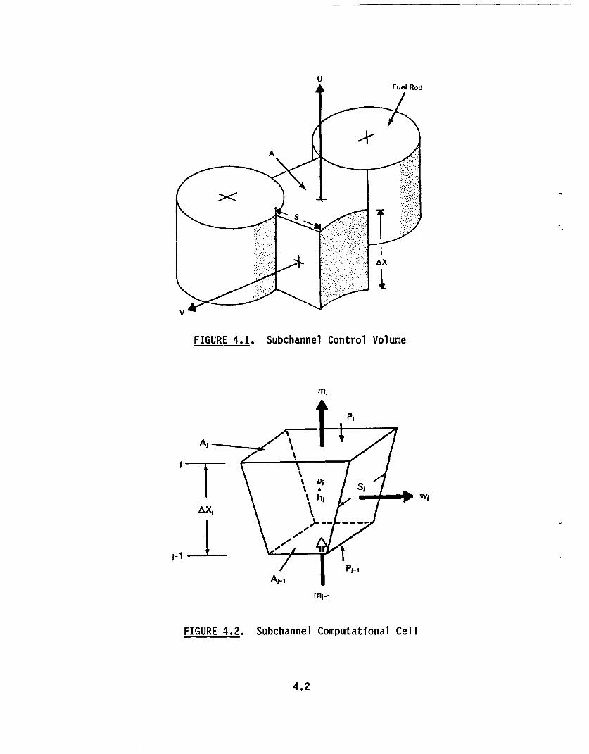
equations is an axial segment of a subchannel as illustrated in Figure 3.1.

To derive the conservation equations, suitable balances are performed on

the typical control volume shown in Figure 3.2. The axial length of the control

volume is denoted by Ax. The axial flow area at the upper and lower surfaces

is denoted by A and the axial velocity by U. Assuming linear variation in

area between the upper and lower surfaces, the node volume is numerically

equivalent to Ax where A is the average axial flow area, (Ax + Ax Ax)/2.

3.1

Storage System

Subchannel

=Y" U

Fuel Assembly Control Volume

FIGURE 3.1. Relation of Subchannel Control Volume to Storage System

U

FIGURE 3.2. Subchannel Control Volume

3.2

Rods A

AIAXXI

(a) (b) (c)

FIGURE 3.3. Possible Control Volume Shapes Using the Generalized SubchannelNoding Approach. (a) Standard Subchannel Noding, (b) LumpedSubchannel Noding, and (c) Noding for Fluid Not in a Rod Array

Lateral flow between adjacent subchannel control volumes passes through

a region between separated solid surfaces. The width of the gap between sur-

faces is S and the lateral velocity is V. Each channel can have an arbitrary

number of lateral flow connections (three in the case of Figure 3.2) to adjacent

channels, and the gap width, S. may vary from connection to connection.

A fundamental assumption of the subchannel formulation is that any lateral

flow is directed by the orientation of the gap it flows through and loses its

sense of direction after leaving the gap region. This allows channels to be

connected arbitrarily since no fixed lateral coordinate is required. This

formulation allows a great deal of flexibility in modeling complex flow pro-

blems, since the cross-sectional flow area of a channel and its connection to

other channels may be arbitrarily defined. Figure 3.3 shows possible control

volume shapes for standard subchannel noding, and for a channel representing

several subchannels and noding for a fluid channel not in a rod array.

3.3

To develop finite-volume equations, the control volume is represented by

the computational cell shown in Figure 3.4, and computational variables are

located as shown. The state variables of density, p, and enthalpy, h, are

defined at the cell center and are indexed by the node number. The axial

flow rate, m; pressure, P; and axial flow area, A, are located at the cell

boundaries and are indexed by the corresponding node and axial level. The

crossflow per unit length, w, and gap width, S, are on the transverse cell

boundaries midway between the axial levels and are indexed by the gap number

and axial level. In the difference equations, the positions of the variables

are indicated by the axial node index (I, J+1, J-1, etc.), where j increases

as you move up the channel.

The fluid is assumed to be incompressible but thermally expandable; there-

fore, the fluid properties, such as density, are expressed as functions of

local enthalpy and a uniform reference pressure.

mI

Ajj

AXA

m;,

Fmp-I

FIGURE 3.4. Subchannel Computational Cell

3.4

The conservation equations are formulated using velocity as the transpor-

tative variable. However, since COBRA-SFS is derived from previous COBRA

versions, the transportation variables are converted to mass flow rate for

this code manipulation. The finite difference form of these equations comes

directly from the integral statements of the conservation principle for the

given control volumes.

3.1.1 Mass Conservation

The control volume used to derive the mass balance equations is given in

Figure 3.5. Applying conservation of mass to the reference control volume I,

shown In Figure 3.5, gives the following finite-volume equation

(~ fit') + Ujp Aj - U_1p A 1

[rate of 1 + massmass storage transported axiall

+ I eik(VkP SkOx) = 0

+ mass transported= 0Laterally

(3.1)

U. P*Aj

AI

1-

Vjp*S&x

FIGURE 3.5. Mass Balance on a Subchannel Control Volume

3.5

where pn is the density at the previous time step and At is the time step.

The summation of crossflows is performed for all connections, k, that are

members of the set, ti, of all transverse connections to subchannel i. Each

lateral flow connection may have a different gap width and flow rate. Here

and in the following equations the channel subscript i has been omitted where

the reference is clear.

The assumptions made in the derivation of the continuity equation are that

the channel area changes linearly with distance over the length of the control

volume; the fluid density is uniform throughout the control volume; the axial

and lateral velocities are uniform over the respective areas, and the lateral

connection width is constant over the length of the control volume.

The axial velocity U is defined as positive in the upward direction (i.e.,

toward increasing values of J). The transverse velocity V is directed by its

gap k such that positive is by definition an outflow from one channel and an

inflow to the other. The convection used to determine the direction is that

a positive velocity is defined to be from channel ii to channel jj, where ii

is the smaller index of two connected channels. To keep track of the sign of

the transverse velocity, the switch function, elk, is used where

1 if the channel index, i, is equal to ii

ik -1 if the channel index, i; is equal to jj

Therefore, elk 1 indicates that positive flow is out of channel i and

elk = -1 indicates that positive flow is into channel i. The donor cell

convention is used for the convected quantities as indicated by the asterisk.

That is

pi Uj if Uj2 0 (3.2)

Pj+i Ui if U 0< 0

3.6

Likewise,

*V Pii Vk if VkŽO0P*V.k i Pyk if Vk < O (3.3)

The axial flow rate is defined to be

mj = p UjAj (3.4)

and the transverse flow rate per unit length to be

Wk = P VkSk (3.5)

The final form of the conservation used in the COBRA-SFS code is

Ax ,nA t _ -m&t i k eik wk= (3.6)

3.1.2 Axial Momentum Conservation

In deriving the axial momentum equation, it is assumed that all irrever-

sible losses can be calculated using suitable friction factors and local loss

coefficients applied to the bulk velocity. Also, it is assumed that pressure

changes linearly along the control volume and that the shear stress on the

fluid from adjacent channels can be neglected. It is further assumed that a

turbulent cross flow exists between adjacent channels that produces no net

mass exchange but does transport momentum laterally at a rate proportional to

that of lateral turbulent energy transport.

Applying conservation of momentum to the control volume shown in Figure 3.6

gives the following finite-volume form of the axial momentum equation

3.7

AxA 7( a + (I

[axial momentum1 +storage j

a) *Aj -1 * Uj.1 i _ il,

[axial momentum 1transported axially]

Ai UJ 1 +

+

E eik(p U)k VkSk Ax + FT

[axial momentum ] + turbulent momentum]transported laterally exchange

Pj_1Ajl - PjAi - P (A 1 - Ad) + FS - Fg (3.7)

[pressure forces] - [wall drag forces] - [body forces]

FT Uj*P*vjS Ax

FIGURE 3.6. Axial Momentum Balance on a Subchannel Control Volume

3.8

By assuming linear pressure variation and defining

PJ = P J P1 (3.8)

2

then the pressure difference is written as

P_1Aj-l - P Ai = P (Ak1 - Ad) + A (P_1 - Pi) (3.9)

Therefore, the pressure force resulting from the area change is cancelled, and

PJ-1AJ 1 - PiAi - P (A_1 - Ad) = A (P_1 - Pa) (3.10)

The shear forces exerted by the walls are expressed in terms of empirical

wall friction factor correlations and local form loss coefficients. This term

is expressed as

F= 1 fAx +K pUjUJA (3.11)

where Dh is the hydraulic diameter, f is the Darcy-Weisbach friction factor

and K is the additional form loss coefficient to account for local obstructions

such as grid spacers.

The only body force considered is the gravity force. This term is ex-

pressed as

Fg = A~x p g cos e (3.12)

where 6 is the orientation angle of the control volume. For 6 = 00, positivegravity acts downward and opposes positive flow. If 0 = 900, the axial flowis horizontal and gravity has no effect on axial momentum.

3.9

In the axial convection of axial momentum, the convected term is combined

with the flow area and defined as

m= (p U) A (3.13)

and

Urm* if Uj >0ifU <

U Ujm+1 if Uj < 0

and the transporting velocity, Up is defined as

U ( J + >i (3.14)

J Aj+l \Pi Pj+1/

where

pj = 1/2 (Pj + pi+,)

For the term defining lateral transport of axial momentum, the convected

quantity (pjUj)* is converted to axial flow rate by multiplying and dividing

this term by Aj or

(P*) ( (3.15)

3.10

and

km *.1(A)IVk A if Vk 2 °

ik Ai k < i

The transporting velocity Vk is defined as

Ok Sk kj+ kl

Pk,J+1/

(3.16)

where

k = 112 (Pi+ PJ)k

turbulent momentum exchange, FT, is modeled using a turbulent crossflow

axial length, WT, as

The

per unit

FT = i elk WT Ami

f AxjjA j

(3.17)

The turbulent crossflow produces no net mass exchange between adjacent channels;

however it does transport both momentum and energy from one channel to another.

The constant of proportion relating turbulent momentum to turbulent energy

transport is fc The variable fc has the same function as a turbulent Prandtl

number. If fc = 1.0, energy and momentum are exchanged at equal rates. If

fc = 0.0, there Is no lateral momentum exchange due to turbulence.

3.11

When the above definitions are substituted into equation (3.1-7) the

final form is

Ax(mj - mn) * _ [At mm U j-1 j-1 keyik(A)kkSk Jix

(e p1A; 1 ) c K (1 (D + ) | mA+ke1 eikwTk fc =j (J1- P 2 D h L Ai... pA m

- AAx p g cos 8 (3.18)

3.1.3 Transverse Momentum Conservation

A transverse momentum control volume for a standard subchannel noding is

shown in Figure 3.7. The gap width between rods is denoted by S and the control

volume length is denoted by -. Due to the predominantly axial nature of the

flow in rod assemblies, the fluid field solution is relatively Insensitive to

the dimensions of the transverse momentum control volume. It is assumed that

the transverse velocity is normal to the transverse gap inside the control

volume.

In deriving the transverse momentum equation, it is assumed that all

irreversible losses can be calculated by the use of a single loss coefficient

applied to the transverse velocity. Also, it is assumed that transverse

momentum is not convected in the transverse direction so that each transverse

momentum control volume is independent of the others.

3.12

Subchannels

FIGURE 3.7. Transverse Momentum Control Volume

Applying conservation of momentum

gives the following finite-volume form

to the control volume shown in Figure 3.8

of the transverse momentum equation

AxSk (P- V)n) +

transverse momentum1 +[storage J

Vs* *_ * *VkVj - P JVlSkuJ-l

[transverse momentum1transported axially]

AXSk(3.19)

= [pressure forces] - [wall shear forces]

3.13

P Vj~S Uj

Plp ,SAx OI

0 (PA-1 SAXI

F..-

* Vl, Sul1

FIGURE 3.8. Transverse Momentum Balance on a Control Volume

The shear forces exerted by the walls and fuel rods are expressed in

terms of empirical local form loss coefficients. The shear force per unit

length, Fs, is expressed as

Fs = -1/2 KGIVI XSP (3.20)

where K is the form loss coefficient.

In the axial convection of transverse momentum,

* * *

Wj= '3V KS (3.21)

the crossflow is used as the convected quantity and the transport terms are

expressed as

3.14

* wi ifii Ž0ui Wi = -

aua w+1 if ui < 0

and the transporting velocity, Up, is defined as

uj = -J(A. 1+A- + _t) (3.22)

When the above definitions are substituted into Equation (3.19), the

finite-volume form used is

/w - no * *S~xg (

ax +Wjuj Wj..Ujj = _ _ - P)j-l (3.23)

- 1/2 KGIpSI w; t (3.23)

3.2 FLOW SOLUTION METHOD

The finite-volume equations presented in Section 3.1 are written for

each fluid node or gap connection in the problem. The RECIRC solution method,

adapted from the COBRA-WC code (George et al. 1980), is used to iteratively

solve the set of equations to obtain the flow and pressure field. The primary

advantage of the RECIRC method is that it is applicable to reverse and

recirculating flows, such as those occurring in natural circulation cooled

storage systems. RECIRC uses a Newton-Raphson technique similar to the one

developed by Hirt (1972) to solve the conservation equations, but it has been

made implicit in time as was done in the SABRE code (Gosman et al. 1973).

Since the solution method is quite complex, it is summarized below before

examining each separate step of the solution method in more detail.

The RECIRC flow field solution routine is divided into two parts: a

tentative flow solution and a pressure solution. The tentative flow solution

3.15

is achieved by iteratively sweeping the bundle from inlet to exit. In each

sweep, the bundle, tentative axial flows, m, and crossflow, w, are computed

by evaluating the two linearized momentum equations with current values for

pressures and other variables. (The specific forms of the momentum equations

will be described in the following pages.) Then, after all tentative flows

and crossflows have been computed at all axial levels, the flows and pressures

are adjusted to satisfy continuity by a Newton-Raphson method. The resulting

flow field from this pressure solution is then used in the energy equation to

obtain an enthalpy and fluid properties distribution for the next axial sweep.

A flow chart of this method is shown in Figure 3.9. The tentative flow solution

is described in more detail in Section 3.2.1 and the pressure solution is

described in Section 3.2.2. The energy solution will be discussed in

Section 4.2.

3.2.1 Tentative Flow Solution

The first step is the solution of the axial and transverse momentum

equations for the tentative flow rates m and w. Since the axial flow in channel

I is affected by axial flows in adjacent channels through the crossflow terms,

the tentative flows, mj, in all channels at an axial level must be solved for

simultaneously. The axial momentum equations are linearized to form a system

of N equations, where N is the number of channels.

[A] ;iJ = - 9cA (P; - P. 1) + B (3.24)

The diagonal elements of [A] are defined by

A.=Ax -k -+ +M1 aE&jUj tj_1 jIk k ik k T1 a Dh Ax)|pA|

wT+ Ax (3.25)ke~i pA

3.16

FIGURE 3.9. Flow Chart of the RECIRC Flow Solution Scheme

3.17

where the switch function, 6, is defined as

=i {6j-1 {~6k =

o if U• 0 0

1 if Uj > 0

0 if Ulii> 0

1 if U < O

o if eikVk ' 0

1 if elkVk > 0

The off diagonal elements

senting channels adjacent

Ain = '(15k elk Vk

of [A] contain zeros except for the columns repre-

to channel i where the elements are defined as

SkAx wT

An Pn An(3.26)

where n = II+JJ-i

In the above definition, the subscript n refers to a channel adjacent to i.

II and JJ represent the channels connected by gap k.

The constant B is the source terms calculated as

B = A~xpg cosl + 2D + Kx I AI mj - (-_,) mj+1 U

+ ( 1--6 i i) mj..1 Uj-1 +Ax n+at mi (3.27)

3.18

The pressures and flow rates in Equation (3.27) are those generated during the

previous pressure iteration, except mij 1 which is a predicted axial flow rate

discussed later in this section. To insure that friction effects have the

proper weight when diferentiating Equation (3.24) with respect to pressure,

the linearized pressure loss is defined as

APf = -1/2 (D +f IPAI (2mj- ; n) (3.28)

Equation (3.24) is compacted to a matrix containing only nonzero terms and

solved by direct elimination at each level.

Once a set of tentative axial flows, m , has been obtained, the tentative

crossflows, w, are calculated. Since the transverse momentum equation does

not depend on crossflows in other gaps, a simultaneous solution is not neces-

sary, and the tentative crossflows in each gap are calculated using the linear-

ized form of Equation (3.23)

[~~c -P)Ax nwj = [ync(P 1 -Pj )i - (1-± ) w +1u + (1-16 _ + ftwJ

+ 1/2 KG I wj AX AX+ u K (3.29)

The pressures and flow rates used in Equation (3.29) are those generated during-I

the previous pressure iteration, except for u a velocity based on the

predicted axial flow rate m; 1 The tentative flow field is determined for

each channel and gap for the complete problem domain by sweeping the assemble

from inlet to exit. Note that at this stage the tentative flows and crossflows

do not, in general, satisfy continuity.

The efficiency of the overall solution can be enhanced if the flow rate

used to define the donor cell axial momentum flux is forced to satisfy

continuity during the tentative flow axial sweep. This is accomplished by

defining a set of "predicted" axial flows m; at level ; that are used to

3.19

evaluate the tentative flow rate at level j+1. The predicted flows are

determined by solving the combined linearized momentum and continuity equations

while assuming that the previous axial level flows are fixed. At level j

only, the continuity error for each cell is calculated as

E = ~Ax /At ('0 _ n) +~ - -m4 1,+ Ax E e we (3.30)j i ) 'i keJ 1k J-1

S ,

where m; 1 and wj 1 are predicted flows calculated at the previous axial level

and mj is the just-computed tentative axial flow. Estimated pressure changes,

6P3, are calculated from the Newton-Raphson expression

am -aw6P3 1 P +E n,j-1 aE - E (3.31)

-6P-1 keJ1 4 n,j-l ~j1

where n = ii+jj-i and the pressure derivatives are the same as those defined

later in the pressure solution section.

Once a set of estimated pressure changes are calculated, the predicted

flows to be used in the donor momentum flux terms for the next axial level are

calculated using

Oamme = m m + 6P (3.32)

- w

Wi ` w- 1 + aP (6PW1ij - 6PjJJ_1) (3.33)

The tentative flows and pressures are not updated using this information. The

predicted flows are used only to provide a better estimate of the donor momentum

flux distribution to the momentum equations at the next axial level.

The predicted average axial velocity in the gap, used in Equation (3.29),

is calculated as

3.20

; + (A + A (3.34)

For forced convection problems, the convergence is substantially improved

if the predicted value for the axial momentum flux is used. For problems with

negative flows or buoyancy-dominated flows, the use of predicted momentum

flux can be counterproductive. The calculation of a predicted momentum flux

is automatically skipped if negative flows occur in an assembly.

3.2.2 Pressure And Linearized Flow Solution

After all tentative axial flows and crossflows have been computed at all

axial levels in all assemblies, the pressures and flows are adjusted to satisfy

continuity. The flow and pressure field in each assembly are locally

independent of all the other assemblies for a given boundary condition.

Therefore, the equations for flow and pressure are solved on an assembly-by-

assembly basis. The first step in this process is to compute the continuity

error, Ej, in all cells using the expression

E. = A. Ax /At (p - pn). + mi - mJ1 + Ax. keg eik w3k i

The adjustments in axial flows and crossflows necessary to satisfy

continuity are defined as

Amj i=i -m (3.36a)

awj= W3 - wj (3.36b)

Am; 1= M mJ1 - Ij-l (3.36c)

where m and w are flows that satisfy continuity.

By substituting these expressions into Equation (3.35) and subtracting

Equation (3.6), the flow adjustments must satisfy the expression

3.21

Amj - A + Ax E eik Awj = -EJ (3.37)

Assuming that m and w are functions of pressure only, the flow corrections

can be expressed as

Am = aP+ aP6 PJ (3.38a)

aw jwAw = l 6Pj,1 + 6p 6l nj-1 (3.38b)

am am 1Am = l P aP 1 j-P2 (3.38c)

where n is the channel adjacent to channel i. The expressions for the flow

and crossflow derivatives are derived from the linearized form of the axial

and transverse momentum equations [Equations (3.24) and (3.29)] and are

presented in Table 3.1.

TABLE 3.1. Flow Derivatives with Respect to Pressure

Flow Derivative Definition(a)

am amgcA 1

ai-i =-apiAi

~ caw awJ S

aPii;;- 1 aPJJij-1 Ci

(a) Aui is defined in Equation (3.25).C; is the denominator Equation (3.29).

3.22

After substituting in these expressions for flow

rearranging, Equation (3.36) takes the general form

damm d am- am- BPJ 2+ I - =J.J + AX

8Pj-2 BP-2 L Pj- 1 8Pj-1 Si eik

correction and

aw;-aP- 6P- _e

ket1

am+BPX '6PJ+ Ax

SI

awE eik BPn

keti n~j-1'5P n'j-1 = E (3.39)

which is equivalent to

aE. BE BE

fP-2 6P-2 + WPi1 -6Pj-1 + B 6Pi +aE

E 8P l nj-1 E;kef1 nj-i

(3.40)

where the 8E/8P terms are given in Table 3.2.

TABLE 3.2. Continuity Error Derivatives with Respect to Pressure

Error Derivative Definition

B E

BP,-1Bmj

WP- BP J-1 + x keOa mj

8wieik BP

I ' -1

BEi8Pj-2 BPJ-2

B E

BP aPj

BEr n j -

kcfj 8Pn,J_

aw- AxJ E etk 8Pj

ni-

3.23

When the above expression is evaluated for all axial nodes M and all

flow channels Q for a given assembly the coefficient matrix consists of N

equations, where N is the total number of cells in the assembly (N = MOQ). The

matrix equation has the form

aEl/ap * * aE/PN P1 1 El

* * =(3.41)

* 00

BEN/BPl * * N/aPN l N EN

Since it is generally not possible to solve a matrix of this size directly,

the matrix is solved in pieces. An alternating direction iterative solution

is implemented that performs a level-by-level sweep followed by a channel-

by-channel sweep for each iteration in the pressure loop.

First, the pressure change in each channel in the assembly is determined

at each axial level using current values of pressure change in adjacent axial

levels. The equation for continuity error becomes

P _ + e n lP = - E 0 E 6P° - Jj 6 0 (3.42)BP i'j1 i'j- kef B nj 1 n,j-1 i B i- 2 p

where 6P0 and 6P? are the recent values of the pressure change at axial

levels above and below the current level, respectively. For all Q channels

in the assembly at axial level j, this equation produces a system of Q equations

having the form

3.24

E BEE~* B p 1 1 B 0

QJi- B 1 Il i |PEl 2 ~J-2 bpi pi

* 0 = 6(3.43)

BE BE * BE BE'. . . -PE :.Qd P0 - :QA BpO

8P1 1J.1 BPQ'j i 1 -QJ-1 Q _i 8%J2 6 '_2 BPJ J

This matrix is solved by direct inversion to obtain new 6P values for the

current level J.

On the second pass the pressure changes at all axial levels are found

for each channel of the assembly using current values for the pressure changes

in adjacent channels. The equation for continuity error is

EE BE BE BEn _6~~P + 6P 4 -E -E - 60BPj- 2 J-2 6P j 1 opj-1 -P J J k1t n l-, (3.44)

where 6P 1 is the current pressure change in adjacent channel n.

Considering all M axial levels, this equation forms a tridiagonal system of M

equations for channel i of the form

6E. Kj. .6. 0 -E 1 + BEi 2

6 6P1,2 .*l ,2 kIe 8Pn, 1 n,

.. 0 0 . .(3.45)

__.._.E E 1 +1 l EE 1M+1 8Et MoBE 1 1+ BP11 ~ iN 1,1+1 ke 1 BP n4 M

which is solved to obtain new 6P values for the current channel.

The pressure solution is a potentially time-consuming process for large

problems. To solve the equation more efficiently, a one-dimensional axial

approximation of the problem is solved after a certain number of level-by-

3.25

level and channel-by-channel sweeps. To form the one-dimensional tridiagonal

matrix equation, the total continuity error at each level is calculated as

QEj = E Eij (3.46)

A tridiagonal matrix is then formed:

[G] {6P} = E (3.47)

where Gij = aE/aPj

which is solved to obtain an average pressure correction, 6Pj, at each level,

which is then applied to the pressures at that level.

During the pressure loop, the computational mesh is repeatedly swept,

level-by-level and channel-by-channel, solving for 6P, until the change in

all of the 6P values falls below a specified convergence criteria.

After the solution to the pressure equation has converged, the resulting

pressure changes, 6P values, represent adjustments to the pressure field that

make the flow field satisfy continuity. The pressures and flows are then

updated using

p =p + 6P (3.48)

. eammJ mi + BP; (6Pili_1 - 6P i,;)349

.. awW= w; + aP j 1 (6P Jj,_. - 6Pjj.j_.) (3.50)

3.26

-

where P 0 is the pressure from the previous outer iteration. The flow solution

now satisfies both momentum and continuity for the current set of properties

and boundary conditions. The method is then repeated for each assembly in the

problem domain. The new flow field is used in the energy solution to determine

the amount of convection heat transfer occurring within the problem. The

energy solution is described in more detail in Section 4.2.

3.3 CONSTITUTIVE FLOW MODELS

To close the system of equations described in the previous sections, a

set of constitutive relationships is required. For example, the friction

factor and form loss coefficients serve to close the momentum equation solution.

The constitutive models presented below are empirical in nature and, therefore,

should be applied with care since they may be valid only over a certain range

of conditions.

3.3.1 Friction Factor Correlations

The shear stress term in the axial momentum equation is expressed in the

form

Fs = 1/2 + Ka (3.11)

where f is the Darcy-Weisback friction factor and K is the form loss coef-

ficient. The friction factor for turbulent flow is obtained from the expression

f = aReb + cRed + e (3.51)

where Re is the subchannel Reynolds number, defined as

mDhRe = Amh (3.52)

and a, b, c, d, and e are specified constants.

3.27

Several friction factor correlations may be input and applied to different

subchannels within the problem. A second friction factor correlation may be

input for laminar flow conditions, which has the form

f = aZRe B + CZ (3.53)

where at, BZ, and CZ are specified constants.

When both turbulent and laminar flow correlations are specified, the

largest of the two friction factors at a given Reynolds number is used in the

axial momentum equation.

The friction factor described above is based on subchannel averaged fluid

viscosities. As an input option, the friction factor may be corrected for

the viscosity variation near a heated surface by using the relationship (Tong

1968)

fcorr + H Pwa l 0.61 (3.54)f Pw [ Lbulk,

where fcorr is the corrected friction factor, f is the friction factor using

bulk fluid properties, PH is the heated perimeter, Pw is the wetted perimeter

and Nwall is the viscosity evaluated at the wall temperature. The wall temper-

ature is calculated from

Twall 2bulk PhH (3.55)

where H is the channel heat transfer coefficient. This correction is based

on the assumption that the total perimeter of the channel consists of two

regions: one heated (Ph) with a uniform flux (designated q') and the other

unheated (Pw - Ph).

3.28

3.3.2 Form Loss Coefficients

Loss coefficients are used to represent additional pressure losses across

grid spacers, orifice plates, and other local flow obstructions in the axial

direction. The pressure drop across an obstruction is expressed as

AP = kmim (3.56)2gCpA

where K is a local loss coefficient.

This formulation can be used to model flow through any sudden contraction or

expansion where the change in flow results in irreversible losses that cannot

be modeled completely with an area change alone. These loss coefficients are

specified as a constant or as a function of Reynold's number in tabular form.

The pressure loss in lateral flow through a gap is treated as a local

loss rather than a wall friction loss. This permits the formulation of the

pressure loss in terms of the known geometric quantities:

=KG 1w wAP = 2~ll (3.57)

2gcpS2

where KG is the transverse loss coefficient.

In rod assemblies, the coefficient KG can be thought of as the form loss

for flow through the gap between two adjacent fuel rods. The value for KG is

dependent on the geometry of the given problem and must be specified through

input.

An additional option exists to specify complete flow blockages in the

axial direction. The blockages are specified by subchannel and axial level.

3.3.3 Turbulent Mixing Correlations

A fluctuating crossflow per unit length, wT, is computed as a fraction

of the average axial flow. The fluctuating crossflow performs an equal mass

exchange between adjacent subchannels.

3.29

The turbulent mixing correlations give the user a choice of four

forms (Rogers and Todreas 1968; Ingesson and Hedberg 1970; Rogers and

1972):

different

Rosehart

1) WT = P'kGo

2)

3)

4)

WT = a RebSk G'

(3.58)

(3.59)

(3.60)Reb D' G'WT = a

WT = a Re - D' G'T Z k (3.61)

where Re = GADAs

D' = 4 (Ail; + Ai)/(PW i+ Pwi)

GI = (Min1 + mj )/(A11 + Add)

The user may specify different correlations or different coefficients for

each assembly type.

3.4 FLOW BOUNDARY CONDITIONS

To solve the system of equations described in the previous sections,

some form of flow boundary condition must be specified. Several types of

boundary conditions are available in the COBRA-SFS code. These boundary

condition options include the following:

* Option 1 - Specify the inlet axial mass flux. This may be a uniform

3.30

axial mass flux for all channels or it may be specified for each assembly

and/or subchannel.

* Option 2 - Specify an average axial mass flux, but have the code split the

total flow so that a uniform pressure gradient exists at the inlet.

* Option 3 - Specify a total axial pressure drop across the system. The

code then determines the inlet axial flow for each channel.

* Option 4 - Specify a total flow and an equal pressure drop across all

channels. The code then splits the total flow to give a uniform pressure

drop across the system.

In all cases an inlet mass flux must be specified. For the first option,

the mass fluxes remain constant. For the second option, a new set of mass

fluxes reflecting a uniform inlet pressure gradient are calculated and are

then frozen. For the third and fourth options, the specified mass flux distri-

bution is used as an estimate until enough information is available to perform

a flow field calculation based on pressure.

The uniform inlet pressure gradient option (option two) is described in

more detail in Section 3.4.1. The total pressure drop (option three) is applied

to all channels in the problem unless pressure losses must be accounted for

in the plenum regions. These losses are modeled using the network model,

which is described in Section 3.4.2. The transient forcing functions applied

to the flow or pressure boundary conditions are described in Section 3.4.3.

3.4.1 Uniform Inlet Pressure Gradient Option

To split the flow for a uniform inlet pressure gradient, an adjustment

is made to the inlet flow, mu, in each channel, so that its inlet pressure

gradient (DP/DX)i, is equal to the average inlet pressure gradient. The pres-

sure gradient is assumed to be proportional to the square of the inlet flow

(DP/DX)1 = Cm12 (3.62)

The change in pressure gradient due to a change in the inlet flow is found by

forming the derivative of Equation (3.62)

3.31

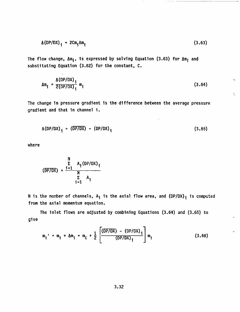
A(DP/DX)1 = 2Cm1Am( (3.63)

The flow change, Am1, is expressed by solving Equation (3.63) for Am1 and

substituting Equation (3.62) for the constant, C.

A (DP/DX),Am1 = 2TDP/DX) ml (3.64)

The change in pressure gradient is the difference between the average pressure

gradient and that in channel 1.

A(DP/DX) 1 = (DPIDX) - (DP/DX) 1 (3.65)

where

(-DP/D-X) =

NE Ai(DP/DX)i

i =1NE Ai

i =1

N is the number of channels, Ai is the axial flow area, and (DP/DX)i is computed

from the axial momentum equation.

The inlet flows are adjusted by combining Equations (3.64) and (3.65) to

give

1 (DP/DX) - (DP/DX)m + Ami 2 (DP/DX) 1 m; (3.66)

3.32

Equation (3.66) and the axial momentum equations are repeated in turn until

the flow change is sufficiently small. This is done immediately after the

inlet flow data is read in, before the main flow solution begins.

To ensure that the total flow is conserved, the adjusted flows are re-

normalized each iteration by

N 0

m = m i=1 (3.67)I I MN

1=1

where mi' is given by Equation (3.66) and mi0 is the initial input inlet flow.

Even though the COBRA-SFS code has not been validated for transient calcu-

lations, the final inlet flow split from a steady-state solution would be

used without further adjustment in a transient analysis. However, the total

flow may change by the input forcing function on the inlet mass flow. The

specified mass flux or total pressure options can be applied in both the steady

state and transient. Since the pressure drop is very sensitive to changes in

inlet flow, the flow split calculation may not converge in transients for

very small time steps or if there are severe changes in the flow field. In

such cases, the inlet flow split must be specified directly.

3.4.2 Network Model

The specified total pressure drop boundary condition is generally applied

uniformly to all channels. However, for many modeling situations, it may be

desirable to allow the code to calculate the flow distribution between assem-

blies based on the orificing and assembly arrangement. The network model has

been developed for the COBRA-SFS code to model the pressure losses above and

below the channel region. When the network model is used, a single pressure

drop is specified as a function of time, and the subchannel flow rates are

adjusted so that the pressure drop through each possible flow path matches

the specified pressure drop.

3.33

Figure 3.10 is a schematic description of the network model for a three-

assembly problem with a bypass channel. The conservation equations described

in the previous section are solved only for the channel region as noted in

Figure 3.10. This channel region formally represents the rod assembly where

flow resistance is given by friction factors and loss coefficients. The

gravitational head is also accounted for In this region. Along the rest of

the flow paths, a reduced momentum equation is solved, which takes into account

only the flow resistance due to friction and form and the gravitational head.

No inertia terms are included. It is assumed that the transport time through

the network model is zero.

In the example described by Figure 3.10, the resistances marked RAIN and

RAOUT would be the flow resistances associated with the assembly inlet orifices

and the outlet hardware (handling socket, etc.), respectively. The loss coef-

ficients can be made dependent on Reynolds number. A gravitational pressure

drop can also be modeled by supplying head lengths at the inlet and outlet.

This is noted as HA in Figure 3.10. The assembly inlet gravitational head is

calculated using the inlet temperature to define the density. The outlet

gravitational head is calculated using the mixed mean assembly outlet temper-

ature.

The assembly group dynamic loss coefficients, RGIN and RGOUT' represent

the flow resistance from a common plenum to assembly group plenums or to the

down corner region. The group dynamic loss coefficients are assumed to be inde-

pendent of Reynolds number. Here too, gravitational losses may be modeled by

supplying head lengths. Finally, RT may represent the dynamic loss coefficient

for flow from the inlet nozzle to the common plenum.

For most problems the actual loss coefficients for each of these resis-

tances will not be known, but the flow and corresponding pressure drop across

each resistance should be available. The effective loss coefficients may then

be calculated as

APgcR= 2 (3.68)

m

3.34

RGOU ou+ H out Ro Rout + HGOU t ReooMit +HGOUt

RAo, + HA { RAOUt + HAOU, RA + HA RAt + HA

!Al Channel Assembly Assembly Assembly Downcomer

APT Region 2 3

Rin + HA~n RA~n + HAM RA +HA RAin + HAin

T + RGn + HGn RI + H} In

FIGURE 3.10. Schematic Description of the Network Model for Pressure Drop Through Reactor Vessel

For RA, which may be dependent on Reynolds number, it is necessary to supply

a wetted perimeter so the Reynolds number can be calculated from the flow

rate. The wetted perimeter need not have any physical significance but should

be chosen so that the correct loss is obtained for a given flow rate when using

the specified resistance versus Reynolds number curve.

3.4.3 Transient Forcing Functions

Even though the COBRA-SFS code has not been validated for transient calcu-

lations, to simulate transients the inlet enthalpy, heat generation, system

pressure, and inlet flows can be specified as a function of time. COBRA-SFS

reads a table of time versus relative (or actual) value for each parameter to

be varied. Linear interpolation is used to obtain values between specified

time entries. The value of parameter P at time t is computed as

P(t) = F(t)P(o) (3.69)

where F(t) is the factor interpolated from the input transient table at time

t and P(o) is the steady-state value of parameter P. Alternatively, the actual

value of the parameter may be used in the table, so that

P(t) = F(t) (3.70)

where F(t) is the value interpolated from the table at time t.

The factors entered in the forcing functions tables apply to any of the

input options available for that parameter. For example, the inlet enthalpy

forcing function table applies to average inlet enthalpy, average inlet temper-

ature, or to individual channel inlet enthalpy or temperature, depending on

the input option selected.

Flow forcing functions may be used with any inlet flow option, including

the uniform inlet pressure gradient option. Alternatively, a forcing function

may be specified for the uniform pressure drop option. If the pressure drop

is specified, a flow forcing function becomes the pressure drop forcing function

and the inlet flows are computed in response to the pressure boundary condition.

The forcing functions do not apply to the total flow boundary condition.

3.36

4.0 ENERGY MODELS AND SOLUTION METHOD

One of the primary objectives of a spent fuel storage system is to remove

decay heat from the fuel and maintain it within certain temperature limits.

The heat is typically removed by a combination of the three primary modes of

conduction, convection, and radiation heat transfer. To predict the temperature

field within the storage system, the COBRA-SFS code must accurately model

each mode.

In this section, the finite-volume energy equations and solution method

are described in detail. The derivation of the conservation of energy equations

for the fluid, solid structures and fuel rods is demonstrated in Section 4.1.

The method for solving the equations is presented in Section 4.2. The con-

stitutive models for heat transfer are presented in Section 4.3. The choice

of thermal boundary conditions are described in Section 4.4.

4.1 CONSERVATION EQUATIONS

A typical spent fuel storage system may be divided into three regions:

the cooling fluid, the solid structure and the spent fuel rods. For a typical

spent fuel dry storage cask the cooling fluid would be the naturally circulating

gas within the cask and the solid structure would be the assembly basket and

cask body. To derive the conservation of energy equations for each of the

regions, an energy balance is performed on the appropriate control volume.

The derivation of the energy balance is presented below for each region.

4.1.1 Fluid Energy

The control volume used to derive the conservation of fluid energy equation

is the standard subchannel control volume described in Section 3.1 and shown

again in Figure 4.1. In a finite-volume formulation, the subchannel control

volume is represented by a computational cell as shown in Figure 4.2. The

computational variables are located on the cell as shown. The state variables

of density (p) and enthalpy (h) are defined at the cell center and are indexed

by the node number. The axial flow rate (m), pressure (P), and area (A) are

4.1

U

v

FIGURE 4.1. Subchannel Control Volume

ml

Al

Ai

WI

i-

mI-i

FIGURE 4.2. Subchannel Computational Cell

4.2

located at the axial cell boundaries and are indexed by the corresponding

node and axial level. The crossflow per unit length, w, and gap width, S,

are placed on the transverse cell boundaries midway between the axial levels

and are indexed by the gap and axial level. In the difference equations, the

positions of the variables are indicated by the axial index, J, J+1, j-1, etc.

The axial and transverse convection terms involve the transporting of

enthalpy, located at the cell centers, by flows defined at the cell surfaces.

It is assumed that the enthalpy being transported is equivalent to that of

the donor cell, i.e., the cell from which the flow originates. For example,

the finite-volume form of the axial convection term is

* *A (pUh)x+Ax - A (pUh)x = mjh -ml h (4.1)

where h is the donor cell enthalpy.

The fluid energy equation is derived by performing an energy balance on

the control volume shown in Figure 4.2 and assuming that flow work is negli-

gible. The balance includes terms describing both axial and lateral convective

transport of fluid energy as well as an energy storage term. In addition,

energy may enter the subchannel fluid from connecting fuel rods, QFR' solid

surfaces, QFW, or by fluid conduction, QFF, and turbulent mixing from adjacent

channels, QFT. The fluid energy balance is written as:

A Ax At + mjh -mjlh +1 eik wjh QFR + QFF+ QFT (4.2)kei

The crossflow, w, is directed by its gap such that positive crossflow is

defined to be from channel ii to channel jJ, where ii is the smaller index.

To account for this, the switch function, eik, is used as multiplier on the

crossflow where

{ I if the channel index, i, is equal to ii

-1 if the channel index, 1, is equal to Jj

4.3

Therefore elk = 1 indicates that positive crossflow is out of channel i and

elk = -1 indicates that positive crossflow is into channel 1. The total heat

entering from the fuel rods is defined as

QFR E PR Oi Ax q (4.3)nexi

where the summation is over the set, Xi, of all rods, n, facing the control

volume, i. PR is the perimeter of the rod n, * is the fraction of the rodperimeter connected to the control volume, and q" is the convection heat flux.

The total heat entering from the connecting solid surfaces can be defined in

the same manner as

Q maI Pw Ax q (4.4)

where the summation is over the set, Ti, of all solid surfaces, m, adjacent to

control volume, i; Pw is the connecting perimeter of surface m; and q" is the

convective heat flux.

For terms in the fluid energy equation that involve convection heat

transfer through the solid surfaces, the surface-averaged convection heat

flux, q", is modeled using a heat transfer coefficient, Hsurft such that

qc Hsurf (Ts - T) (4.5)

where Ts is the rod or slab surface temperature. Therefore,

Ax I PR 1 q =Ax I PR J Hsurf (Tcn T) (4.6)neX R i c neX R1 srf(cn

and

Ax I P q" =Ax m P H (T - T) (4.7)MET 1 m'ri w W Wm

4.4

where Tc and Tw are the clad and slab temperatures, respectively. When a rod

model is not used, q" is simply

Af

c PR(4.8)

where Af is the cross sectional area of the fuel and q'" is the volumetric

heat generation rate of the fuel.

The total heat entering by fluid conduction from adjacent subchannels is

defined as

FF= E SAx q" (4.9)ken j

where the summation is over all gaps, k, connecting the control volume, i, S

is the gap width, and qjk is the fluid conduction heat flux.

The heat flux from fluid conduction, q", between adjacent subchannels is

based on the gap width, S, and conduction length, Zc, defined as

Qc = Zk (4.10)

where . is the transverse control volume length and Zk is an empirically deter-

mined conduction shape factor. Equation (4.9) then becomes

QFF = AX E Sk q" = Ax E Skeikkk (Q - (4.11)key ket k ikk PZk

where kk is the average fluid thermal conductivity based on channel fluid

temperature from the previous iteration.

Turbulence in the flow field mixes the fluid in adjacent subchannels

through the gap. This mixing results in the transfer of fluid energy from

one subchannel to another. To determine the amount of transfer that occurs,

4.5

a turbulent exchange crossflow, WT, is calculated as a function of flow and

other parameters. A selection of different expressions used to calculate the

turbulent exchange crossflow is described in Section 3.4.3. The turbulent

energy exchange between subchannels is expressed as

QFT e wT (hi - h.) (4.12)

When all the terms are combined, the following conservation of fluid

energy equation is obtained:

A Ax ph - (,h) +At mjh 'm-1h + E e ik wjh

nergy storage + energy transport + energy transporte[ + axiallyr laterally

Ax I PR hi Hsurf (Tc T) +Ax E Pw Hw (T -T)nex. n METn WM

= [rod heat input] + [slab heat input]

+ Ax E ek Sk kk + e eik wT (hij - hjj)k (4.13)kEik Skk k keti

+ [fluid conduction laterally] + [turbulent energy exchange]

In this derivation, it is assumed that there is no fluid conduction in

the axial direction. All other forms of energy that are not explicitly repre-

sented in Equation (4.13) (such as potential and kinetic energy) are assumed

to be negligible.

4.1.2 Solid Structure Energy

Conduction through solid structures plays a significant role in many

heat transfer problems. For a dry storage cask, heat is removed by conduction

4.6

through the assembly basket and cask body. Therefore, an equation for the

conservation of energy in solid structures is required to model the solid-to-

solid and solid-to-fluid heat transfer.

The control volume used in the solid conservation of energy equation,

which hereafter will be referred to as a "slab", is shown in Figure 4.3. The

axial length of the control volume is denoted by Ax, which corresponds to that

used for the fluid subchannels, and the cross-sectional area is denoted by A.

The control volume may have any number of surfaces connected to adjacent slabs

or fluid subchannels in the lateral direction. In addition to conduction and

convection heat transfer, the control volume may exchange energy by thermal

radiation with the surfaces of fuel rods and other slabs. The slab control

volume is similar to the subchannel control volume in that it allows a great

deal of flexibility in modeling heat transfer problems, since it is not con-

strained by a fixed coordinate system.

A QAX-

- -

_0* OWW

QWW

AWF

TwQFW

QRW

FIGURE 4.3. Solid Control Volume

4.7

The slab conservation of energy equation consists of an energy storage

term and a series of terms describing energy transferred from subchannels,

other slabs and rods. The total energy from adjacent subchannels, QFW1 is

transferred soley by convection. The total energy from other slabs, QWW is

transferred by both conduction and radiation. The total energy from fuel

rods, QRWI is transferred solely by radiation. When these terms are added,

the conservation of solid energy equation may be written as:

Tw - T. n

A Ax Pwcw At = QFW 0 QWW - QRW (4.14)

where Tw is the slab temperature.

Using the definitions provided in Section 4.1.1, the total energy from

adjacent subchannels is described by

QFW AX E PwHw (Tw Tz) (4.15)ZE~i

where the summation is over the set, fi, of all subchannels, Z, connected to

slab control volume i; Pw is the wetted perimeter; and Hw is the heat transfer

coefficient.

The total heat entering the reference control volume, i, from adjacent

slabs by conduction and radiation is defined as

QW =E A qj + E A q (4.16)QW C AWW qk Ma AWF qRW +QAX (.6mesama

transverse + [radiation] + [axial conduction]conduction

where the summation in the first term is over the set, i, of all slab control

volumes m, with a conduction connection to control volume i; Ai is the

connecting area; and q" is the conduction heat flux.

4.8

Radiation is assumed to be confined to two dimensions so that only the

slab and fuel rod surfaces on the current axial level are considered. The

summation in the second term is over the set, ci, of all slab control volumes,

m, connected to the control volume i, by radiation. AWF is the radiations

surface area of slab I and q" is the net radiation heat flux from the slab.

In addition to heat transfer in the lateral direction, the heat transferred

in the axial direction by solid conduction is defined as

QAX = (A q") + (A q") (4.17)

where surface A is the slab cross-sectional area and qu is the axial conduction

heat flux at the top and bottom surfaces.

The solid conduction between adjacent slabs, q", is modeled using a

composite thermal conductance, U, which accounts for the heat transfer area,

the thermal conductivity of the slab materials, and any gap resistance or

thermal radiation at the slab interface. Therefore,

I AWW q" = E U (Tw Tw) (4.18)

and

(A q")j + (A q")J-1 = U (TW- TW ) + U;_1 (T T (4.19)x j+1 J- i-i

where Uj and U J 1 are the composite thermal conductances through the top and

bottom of the slab, respectively. The calculation of composite thermal con-

ductances, U, is described in more detail in Section 4.3.3. The total heat

entering from fuel rods by radiation is defined as

QRW Nat AWF qR (4.20)nerL R

4.9

where the summation is over all fuel rods, n, connected to the control volume,

i, by radiation. AWF is the radiations surface area of slab i and q is the

heat flux from each rod.

The radiation heat transfer from one surface to another is calculated

using the expression

qR= a F1 2 (T4 - T4) (4.21)

where F1-2 is the gray body radiation exchange factor based on geometry and

surface emissivities and o is the Stefan-Boltzmann constant. Using this ex-

pression, the radiation heat transfer from slabs and rods is

E AWF q"= E AWF Fim (Tw4 _ T) (4.22)mew; mea W m

where TWm is the temperature of slab m, and

E AWF qRR nE AWF a Fin (Tw4 Tc 4) (4.23)

ne ei n

where Tc is the cladding temperature of rod n. The calculation of radiation

exchange nfactors, F, is described in detail in Section 4.4.4.

4.10

When all the terms are combined, the solid structure energy conservation

equation is

T- Tn

A Ax c ft w = U (Tw T ) U 1 (T T )w At i w~j+i. - w-

[energy storage] = [axial heat conduction]

- E U (Tw T ) - i a Fim (Tw Tw)

- lateral heat - radiation heat transfeonduction rom slabs t

- I A F 4(T T) - Ax I Pw Hw (Tw - TO) + Ax A q.". (4-24)neiWF in cn LE ~)+xq'' (.4

radiation heat transfer- onvection hea + [heat generation]from rods t [transfer h

4.1.3 Rod Energy

The spent nuclear fuel rods in storage generate decay heat that must be

efficiently removed to maintain acceptable fuel rod temperatures. The heat

transfer from the rods is modeled in three different ways.

The first, which is the simplest method of distributing the heat generated

in a fuel rod, is to assume a constant heat flux around the periphery of the

rod while neglecting transient effects and thermal radiation. The total heat

is distributed to the surrounding channels according to the fraction of the

rod perimeter, Op, adjacent to each channel so that the convection term in the

fluid energy Equation (4.3) for channel E becomes

0F-1 P Ax q" (4.25)QFR = E PR Q x c (.5tEC-Y

4.11

where q" is simply

Afq1= f q (4.8)

r

and Af is the cross sectional area of the fuel and q" ' is the fuel volumetric

heat generation rate.

The second method is used for most steady-state spent fuel problems where

the effect of thermal radiation is important. This rod model was developed

to provide clad surface temperatures for determining convection and radiation

heat transfer.

The total heat removed by convection is defined as before in Equation

(4.25) but q" varies as a function of fluid temperature [see Equation (4.5)].

The radiation term includes contributions from slabs and other rods within

the same assembly. By assuming that only slabs and rod surfaces on the same

axial level exchange radiant energy, the net radiant heat transfer from other

fuel rods by radiation is defined as

IRR =EP Ax (q") (4.26)

where the summation is over the set, 5j, of all fuel rods within an assembly

radiating to rod i, PR Is the rod perimeter, and (qr)n is the net radiant heat

flux from each rod. The total heat flux entering from slabs by radiation is

defined as

IRW =E P Ax (q") (4.27)QR xmep1 R

where the summation is over the set, pi, of all slabs, m, connected to rod i

by radiation. The term (q")m is the net radiant heat flux from each slab.

The rod energy conservation equation for the second model takes the form

4.12

0 - Ax I PR Hsurf (Tc T) Ax P F (T 4T4)

- Convection heat transfers - [radiation heat transfewith fluid between rods

Ax E P Fim (T4 T4 ) + A Ax q'"' (4.28)

-[radiation heat transfe + [heat generation]from slabs

where Af is the cross-sectional area of the fuel and q" ' is the fuel volumetric

heat generation rate. In this derivation, it is assumed that there is no axial

heat transfer, and that the temperature is uniform around the circumference

of the cladding.

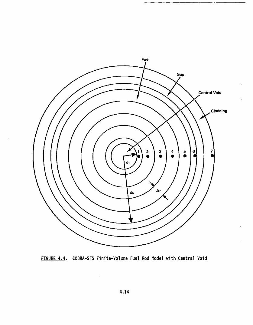
The third model is used for transient calculations. In this model,

separate energy equations are written for the clad and the fuel energy. The

fuel rod is divided into one clad node and several fuel nodes as shown in

either Figure 4.4 when a central void is present or Figure 4.5 when there is

no central void. The innermost and outermost fuel nodes are one-half the

thickness of the other nodes. The cladding energy equation is obtained by

performing a lumped energy balance on the cladding material at each axial

level. The clad energy conservation equation is written as

4.13

Fuel

FIGURE 4.4. COBRA-SFS Finite-Volume Fuel Rod Model with Central Void

4.14

Fuel

FIGURE 4.5.. COBRA-SFS Finite-Volume Fuel Rod Model Without Central Void

4.15

T~ -TA a pC~ -1 PR *Ax q" - I Ax q.A x^ pC At c =-£i PR Z0 xc nesti R r

[energy storage] = convection 1- prod radiationheat transfer heat transfer

- E P Ax q" - PfAx q1 (4.29)

- [slab radiation1 - [heat transfer from fuel]Lheat transfer

where Pf is the perimeter of the fuel and q; is the surface averaged heat

flux across the gap. The only term not defined in the composite rod model is

the heat transfer from the fuel to the clad. The fuel surface-averaged gap

heat flux, q%, is modeled using a gap heat transfer coefficient, Hg, such that

q- Hg (T - T (4.30)g H c I'sf5

where dfuel is the fuel diameter and Tfs is the fuel surface temperature.

Solid conduction within the fuel is modeled in both the radial and circum-

ferential directions with the variable No indicating the number of circumfer-

ential sections the fuel rod is divided Into. The temperatures

are identified as Tk m where k is the radial location and m is the circum-

ferential location. The finite-volume equations for each of the N fuel nodes

and the cladding node, N+1, are as follows:

4.16

Node 1 (inner node):

Pfcf Ti I + id2 kf (T1 m - T2 m)ir

2ArNe+ G-(d+ kf (2Ti m - Tlml - Tlm+i) (4.31)

= qj'' I + N d1 qI

Nodes 2 through N-1:

|P CTkmI.Ldk kf (T

ArN0 km- Tk m) + (Tk,m -Tk+1,m)

2ArNk+ r~k+ d- kf (2Tk~ ~ k,m-1

- Tkm+1) = q' of (4.32)

Node N:

PfCf tNm tNmJrrdN

+ ArN6kf (T -

TN-lm) + N (TdNl - T.Na (~m cm

2ArNe

r(dfuel dN)(2Tntm - Tn,m-1

-d2 dT-T = q I fuel- Nni~m+l' q 4Ne (4.33)

4.17

Clad Node:

dclad - (dclad -2tcla Tc m Tc+m dfuelHg (T T )4N0 c c at N0 cm N,m

AdcladHsurf ArN kc+ N (Tcm Tfluidm) + c (2Tc'm TcM-1 Tcm+i)c0m ruFclad - tclad) c~

•~ E aF (T4 T4 ) + I:P aF (iT 4 _ T =0 (4.34)+ IR in cem cn mEflR i° m cm w,m

In this derivation it is assumed that there is no axial heat transfer, the heat

is generated uniformly throughout the fuel at a given axial location and the

fuel properties do not vary with the radial variation in temperature.

4.2 ENERGY SOLUTION METHOD

The finite-volume energy equations presented in Section 4.1 are written

for each channel, rod, and structural node on an axial level. The energy

solution is divided into three parts: 1) the coefficient matrices representing

the individual rod equations are decomposed by lower-upper (LU) triangular

factorization to determine Tclad as a function of Tfluid' 2) the fluid and

slab equations are solved simultaneously using successive overrelaxation to

obtain a fluid enthalpy and slab temperature distribution, and 3) the rod

temperature distribution is determined by back substitution of the new fluid

temperatures. The rod coefficient matrix factorization is described in more

detail in Section 4.2.1 and the fluid and slab energy solution is described

in Section 4.2.2.

4.2.1 Rod Energy Equation Decomposition

To expedite the energy solution, the rod surface temperature is described

as a function of fluid temperature in the form

Tclad = K1 + K2 + K3 Hsurf Tfluid (435)

4.18

where the constants K1, K2, and K3 are generated by performing an LU

decomposition on the fuel rod finite-volume equations. If radiation heat

transfer is not considered, the constants are generated only once. If radiation

is considered, the clad temperature of a particular rod is dependent on the

temperatures of other rods and the rod equations are solved iteratively using

the fluid and slab temperature distribution from the previous fluid temperature

iteration. When the constants K1, K2, and K3 have been determined, the

expression for clad temperature [Equation (4.35)] is substituted into the

fluid energy equation [Equation (4.13)] prior to solving the fluid and slab

energy equations.

In order to perform the decomposition, the fuel rod finite-volume equations

[Equations (4.31) through (4.34)] are cast into a tridiagonal matrix of the

form shown in Equation (4.36). Here a rod model with one clad node and four

fuel nodes is used as an example.

A12 A13 0 0 0 Tl Y

A2 1 A2 2 A2 3 0 0 T2 Y2

o A3 1 A32 A3 3 0 T3= Y3(4.36)

o 0 A4 1 A42 A4 3 T4 Y4

o 0 0 A5 1 A52 Tclad Y5 + f(Tf

The elements are ordered in a manner that allows storage of the coefficients

in a 3 x 5 array. Thus the subscripts are the index values of the storage array

in COBRA-SFS rather than the matrix index.

The terms in the coefficient matrix A are defined in Table 4.1 and the

terms in the source vector Y are defined in Table 4.2. If the coolant temper-

ature distribution Tf was known, Equation (4.36) could be solved for the rod

temperature distribution. However, since Tf is unknown, matrix A is factored

into a lower ICI and upper IBI triangular matrix as shown in Equation (4.37).

Again the subscripts represent storage locations rather than matrix indices.

4.19

A z

1

C21

0

0

0

0

1

C3 1

0

0

0

0

1

C4 1

0

0

0

0

1

C51

0

0

0

0

1

B11

0

0

0

0

B12

821

0

0

0

0

822

B31

0

0

0

0

B32

B41

0

0

0

0

B42

B51

(4.37)

Performing the indicated matrix multiplication gives:

811

C21 Bil

0

0

B12

C2 1B1 2 +B21

C31B

0

0

822

C3 1B224B31

C41B31

0

0

B32

C4 1B3 2+B4 1

C5 1B4 1

0

0

01

(4.38)am

B42

C5 1B4 2 B510 0 0

By inspection, the terms of

the B and C matrices as:

the stored A matrix can be defined in terms of

A21 = C21B

A3 1 = C3 1B21

A4 1 =41 31

A5 1 C51B41

A 1 2 =B 1 1

A22 = 21 12 21

A3 2 = C3 1 B2 2 +B3 1

A1 3 = B12

A2 3 = B2 2

A33 = B32

A43 = 842

A53 = 0

(4.39)

A4 2 =

A5 2 =

C41B32 +B41

C51B42+B51

4.20

FIGURE 4.6. Flow Chart of Energy Solution Scheme

4.21

TABLE 4.1. Definitions of Coefficients in the A Matrix

El ement Definition

A12

At(d -d2 4N void)

0 N

d2

ArNa f

4ArNkf+ 2

w (d1+d 2)

A 13 d2- ArN kf

A21 and A31 diA rN9 kf

A22 and A32(PC)f (d2 - d2

_ \ 4+1 /At 4N9+ kFF (d1 + di+i) +

Ar0 i i~.

4ArN kf

12(d 1 + dj+1)

A23 and A33

A4 1

di+1- ArN kf

dNA rN9 kf

A42 (PC)f

At

(d2 - d2( fuel N4N0

dN

ArN9kf+dfuelHg+

kf + N0 +4ArN0 kf

1 (dfuel+ d

A43 and A51dfuelHNN9

A5 2

(PC)cladAt

[ ciFd2 (d clad - 2tc1ad)c i a d ] +a

df dcladHsurfN + N

6 Na

2ArNdkc

Y (dclad - tclad)

4.22

TABLE 4.2. Definitions of Terms in the Y Matrix

Element Definition

Y1[(pC)f T q

At + qf

+ 2hrNelf

r2(d 1 +d2)

. dr- - de-r + dvod nl~d void + idvoi

J\ 4 N6 / N Tvo

Y2, Y3 and Y4 At+ qf"] (Tn mi1 + Tn 1m+l)

Y5[ (PC)f clad - (dclad 2tcad)1

At 4N-

ArNekc

f2(dclad- t (T c,m+l c,m-l)

- tclad) c m+c m-

f(Tf) (d5 Hsurf Tfluid)

Using elementary matrix algebra an algebraic expression relating Tclad and

Tfluid can be determined:

let

and

AT = Y

Y = CZ

then CBT = Y (4.40)

CBT = CZ

thus BT = Z

Since B is upper triangular, only Z must be found to solve for T. The elements

of C and B are given below:

4.23

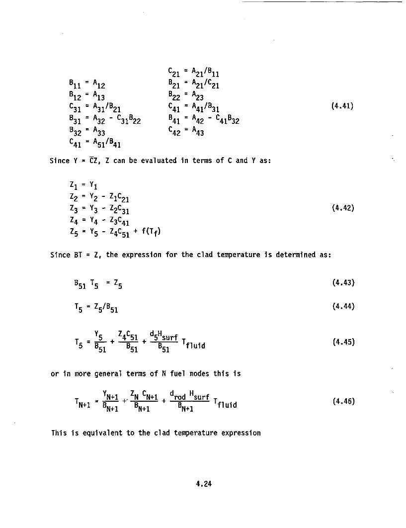
Bl1

B12

C31

B31B32

C4 1

= A1 2

= A1 3

= A3 1 /B21

= A3 2 - C31B22

= A33

= A51 /B41

C21B21

B2 2

C41

B4 1

C4 2

= A21 /B1

= A21 /C21= A2 3

= A4 1/B3 1

= A4 2 - C41B32

= A43

(4.41)

Since Y = CZ, Z can be evaluated in terms of C and Y as:

Zi = YiZ2 = Y2 - ZlC21

z3 = Y3 - Z2C31

Z4 = Y4 - Z3C41

Z5 = Y5 - Z4C51 + f(Tf)

(4.42)

Since BT = Z, the expression for the clad temperature is determined as:

B51 T5 = Z5 (4.43)

T5= Z5/B 51 (4.44)

Y5 + Z4 C515 B51 B51

+ dHsurfT.

851 (4.45)

or in more general terms of N fuel nodes this is

YN+1 N N+1 + drod HsurfN+1 BN+1 BN+1 BN+1 fluid

This is equivalent to the clad temperature expression

(4.46)

4.24

Tclad = K1 + K2 + K3 Hsurf Tfluid (4.35)

This decomposition allows the clad and fuel temperatures to be expressed

as functions of fluid temperature. If there is no thermal radiation heat

transfer, circumferential conduction heat transfer or rod-to-rod contact in

the problem, the rod solution is complete. However, if any of these effects

are included, a change in temperature results in a change in the source matrix,

Y, which requires iteration on the rod temperatures. When the constants K1,

K2, and K3 have been determined, the expression for clad temperature

[Equation (4.35)] is substituted into the fluid energy equation

[Equation (4.13)] prior to solving the fluid and slab energy equations.

4.2.2 Fluid and Slab Energy Solution

The finite-volume formulations for the fluid energy equation

[Equation (4.13)] and the solid structure energy equation [Equation (4.24)]

are written for every fluid and slab node at a particular axial level. The

two sets are generally tightly coupled so that simultaneous solution of both

sets is required. The construction of the matrix equation for each set is

described below. A description of the solution for both sets follows.

The fluid energy equation [Equation (4.13)] is written in terms of fluid

enthalpy. However, certain terms require the fluid temperature to calculate

heat transfer due to fluid conduction and convection. The fluid temperatures

are related to enthalpies by the following approximation.

h - hT =T + h (4.47)

where the reference temperature and enthalpy are chosen arbitrarily as the

previous iteration values for T and h, and c is the fluid specific heat. The

clad temperature, Tc, is represented by the expression developed in

Section 4.2.1.

Tclad = + K2 + K3 Hsurf Tfluid (4.35)

4.25

When these two expressions are substituted into the fluid energy equation

[Equation (4.13)], an equation is obtained that is linear in enthalpy. These

equations, one for each subchannel at level J, are combined to form the matrix

equation

[LI {hi} = {Shl (4.48)

where [L] is an NxN coefficient matrix (N being the number of channels), {ShI

is the source vector, and {hlj the fluid enthalpies at level J. For large

problems the matrix [L] is sparse, therefore only the nonzero elements are

stored.

The only temperature term in l

expressed in terms of enthalpy is l

are obtained during the iteration l

sented in the source vector, IShS.

terms containing slab temperatures

values.

the fluid energy equation that is not

the slab temperature, Tw. These temperatures

from the slab energy equation and are repre-

After each slab energy iteration, the

are updated to reflect the current iterate

The slab energy equation presented in Equation (4.24), is written in

terms of temperature. However, the terms describing radiation heat transfer

are a function of temperature to the fourth power. Rather than treat these

terms explicitly, they are written as

QR AWF O[meo' Fim T- TwJ+ I

nexcF i 4n T4 )]

AWF ° [w (mro Fim + Eimnex1F) e

11eO1iFim T4 + E

im i nxF T4)1

= AWF a HRAD (Tw - T) (4.49)

4.26

where H efT3

T= (mE fm T 4 + I Fi T4 /wt3

ew (moj Finm+ n Fin)

When HRAD and T are evaluated using current iterate values and this linearexpression is substituted into the slab energy equation [Equation (4.24)], an

equation that is linear in temperature at level J Is obtained. These equations

having this form for every slab at level J are combined to form the matrix

equation

[U] (TWI = {SW) (4.50)

where [U] is an NxN coefficient matrix (N being the number of slabs), {SW} is

the source vector, and {Tw}j is the slab temperature at level J. For large

problems the matrix [U] is sparse, therefore only the nonzero elements are

stored.

The slab energy equation consists of terms containing not only slab

temperatures, but also fluid temperatures, Ti, and composite radiation

temperatures, T. Fluid temperatures are obtained from the fluid energy equation

and are represented in the source vector, (SW}. After each fluid energy

iteration, the source terms containing fluid temperatures are updated to reflect

the current iterate values. The composite radiation temperature, T, is derived

as a summation of terms containing slab and clad temperatures to the fourth

power. The clad portion of T is not updated during the fluid and slab solution.However, the slab portion of T is updated after every slab energy iteration.

Both the fluid and slab matrix equations are solved by successive over-

relaxation with a default relaxation factor of 1.2. A single iteration consists

of one sweep through the fluid equations followed by one sweep through the

4.27

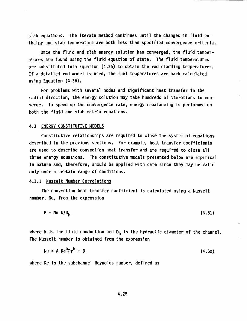
slab equations. The iterate method continues until the changes in fluid en-

thalpy and slab temperature are both less than specified convergence criteria.

Once the fluid and slab energy solution has converged, the fluid temper-

atures are found using the fluid equation of state. The fluid temperatures

are substituted into Equation (4.35) to obtain the rod cladding temperatures.

If a detailed rod model is used, the fuel temperatures are back calculated

using Equation (4.36).

For problems with several nodes and significant heat transfer in the

radial direction, the energy solution may take hundreds of iterations to con-

verge. To speed up the convergence rate, energy rebalancing is performed on

both the fluid and slab matrix equations.

4.3 ENERGY CONSTITUTIVE MODELS

Constitutive relationships are required to close the system of equations

described in the previous sections. For example, heat transfer coefficients

are used to describe convection heat transfer and are required to close all

three energy equations. The constitutive models presented below are empirical

in nature and, therefore, should be applied with care since they may be valid

only over a certain range of conditions.

4.3.1 Nusselt Number Correlations

The convection heat transfer coefficient is calculated using a Nusselt

number, Nu, from the expression

H = Nu k/Dh (4.51)

where k is the fluid conduction and Dh is the hydraulic diameter of the channel.

The Nusselt number is obtained from the expression

Nu = A ReaPrb + B (4.52)

where Re is the subchannel Reynolds number, defined as

4.28

mDhRe = Ap (4.53)

and Pr is the fluid Prandtl number. Two correlations can input for each channel

type and the largest of the two, based on local Reynolds and Prandtl number,

is used for computing the heat flux.

4.3.2 Fluid Conduction Shape Factor

The fluid conduction heat flux between adjacent channels is characterized

by the gap width, S, and a conduction length, Zc, defined as

Zc = P/GK (4.54)

where £ is the transverse momentum control volume length and GK is an empiri-

cally determined conduction shape factor. Doubling the value of GK effectively

doubles the radial fluid-to-fluid conduction heat transfer. Note that 1/GK =

Zk is used in the fluid energy Equation (4.13). The optimal value of GK is

very problem dependent. Experience has shown that for light water fuel

assemblies, GK should be chosen to make P-c approximately equal to the subchannel

centroid-to-centroid distance.

4.3.3 Solid-to-Solid Conductances

The solid conduction between adjacent slabs is modeled using a composite

thermal conductance, U, which includes the heat transfer area, the thermal

conductivity of the slab materials and any gap resistance or thermal radiation

at the slab interface. The components that make up the total thermal resis-

tance between two adjacent slab nodes are shown in Figure 4.7. The terms R,

and R2 denote the thermal resistances from the center of the slab to the slab

interface and account for the slab geometry and material conductivity. The

total series resistance from the slab material is

RSOL = R1 + R2 (4.55)

4.29

where R = L/Ak and L is the conduction length and k is the thermal conductivity

of the solid node. This is the total resistance between two slabs unless there

is a gap at the slab interface.

Heat may be transferred across a gap between the two slabs by conduction

through the fluid or by thermal radiation. The radiation heat transfer is

modeled using an approximate thermal resistance for radiation between gray

parallel plates, given by

1/e1 + l/e2 - 1

RRAD 2 2 (4.56)4 a A (T2 + T 2)(T1 + T 2 )

where T, and T2 are in degrees Rankine and el and e2 are the surface

emissivities of the two slabs. This resistance, along with the thermal resis-

tance for conduction through fluid in the gap, is used to calculate a total

gap thermal resistance using the expression

R 1 1 (.7RGAP RRAD +RCON (4.57)

The overall thermal conductance between adjacent slabs, U, is given by

RSOL RGAP (4.58)

4.3.4 Radiation Exchange Factors

The radiation heat transfer between rod and slab surfaces is modeled

using radiation exchange factors. The net rate of radiant energy outflow

from surface i to surface j, Qij, is defined in terms of an exchange factor,Fii, as

4 = A_ Fj (Tj - Tj4) (4.59)

4.30

Gap

Solid Node #1 Solid Node #2

Conductivity k 1 RRDConductivity k2

VRV R2

| Lt' I RCONLI

Conduction Length Li Conduction Length L2

FIGURE 4.7 Solid-to-Solid Resistance Network

The quantity Fj specifies the fraction of the total amount of radiant energy

emitted from surface i that reaches surface J and is absorbed. This includes

all the paths by which radiation may reach surface j from surface i, including

the direct path and paths of single or multiple reflections. This differs

from the blackbody view factor, Fij, which does not account for reflections.

For all black surfaces (e = 1.0), the two quantities are the same.

The radiation exchange factors, Fly are calculated from the geometry of

the problem and the emissivities of the participating surfaces using the fol-

lowing set of equations (Cox 1977).

i Fki ) Fj = - FkJEj;j = 1,...,n; k = 1,...,n. (4.60)

where Fki and FkJ are the blackbody view factors, e. is the emissivity of

surface i. 8ki is the Kronecker delta, and n is the number of surfaces in an

enclosure.

4.31

The radiation exchange factors used in the COBRA-SFS code can be obtained

in two different ways. For radiation enclosures that do not involve a rod

assembly, the blackbody view factors and surface emissivities are read directly

into the input and radiation exchange factors calculated within COBRA-SFS.

For radiation enclosures that include a rod assembly, the radiation exchange

factors are read from a separate input. An auxilliary computer code, RADX-1,

is used to generate the blackbody view factor array and to calculate the

radiation exchange factors for unconsolidated spent fuel assemblies. This

method is described in detail in the Appendix.

4.4 THERMAL BOUNDARY CONDITIONS

To solve the system of energy equations described in the previous sections,

thermal boundary conditions must be specified. A typical COBRA-SFS model

consists of three regions: an upper plenum, the channel region, and a lower

plenum. For the channel region, thermal boundary conditions are applied to

the outer solid structure nodes at each axial level. Boundary conditions for

the plenum regions are applied in the axial and radial directions for both

plenums. The expression for heat transfer used in these boundary conditions

may include conduction, thermal radiation, and/or natural convection. The

side thermal boundary conditions are described in Section 4.4.1. The thermal

boundary conditions for the plenum regions are described in Section 4.4.2.

4.4.1 Side Boundary Conditions

The fluid and solid structure and fuel rod energy equations for the channel

region were developed in Section 4.1. When no side thermal boundary conditions

are specified, the outside boundary at each axial level is assumed to be

adiabatic. A boundary condition is specified when heat is to be transferred

to some specified boundary temperature.

4.32

At each axial level, a one-dimensional thermal connection is made between

each outside surface node and a boundary temperature. Each connection may

consist of one or a series of radial "regions", with each region having a

different expression for heat transfer. The heat transfer rate through each

region is expressed in the form

qboundary= C1 2 (Ti - Ti+l) (Ti - Ti+) +° (E+7 L - 1 _(T -T 1boudar Vi~l 1+ 'i 11i+

where

Cn = user defined constants

Ti = temperature for boundary region i

o = Boltzmanns' constant

ci = surface emissivity for boundary region i.

This expression is more general than those used in the energy equations de-

scribed in Section 4.1 in that it allows the modeling of heat transfer modes

that are not linear in temperature (such as natural convection, that is ex-

pressed in terms of a Grashof or Rayleigh number).

Boundary temperatures are input as a set of axial profiles that are

assigned to each solid structure node at the boundary. In this way, the

boundary temperatures can vary both axially and circumferentially.

Before the rod, fluid, and slab energy equations at any axial level are

solved, the temperatures in the boundary regions are estimated using slab

temperatures from the previous iteration. The one-dimensional series of

equations for each boundary connection is solved iteratively for a radial

temperature distribution in the boundary region. After the boundary solution

has converged, a linear composite resistance is constructed to represent the

total connection between the outermost slab node and the specified boundary

temperature. This resistance and the boundary temperature are then implemented

in the solid structure energy equation [Equation (4.24)]. After all boundary

4.33

resistances at an axial level have been computed, the energy equations for

that level are solved.

4.4.2 Plenum Boundary Conditions

In a COBRA-SFS cask model, the fluid in a hot assembly flows upward until

it enters the upper plenum region at the top of the cask. The flow is then

assumed to mix with all the other fluid entering the plenum. Heat is lost to

the environment through the top and sides of the plenum region. The fluid

then flows downward through the cooler assemblies until it reaches the lower

plenum.

The plenum regions are only used in problems where flow recirculation

occurs. The primary purpose of the plenum model is to determine the enthalpy

of fluid returning to the channel region.

Each plenum has an axial and radial one-dimensional thermal connection

between the fluid in the plenum and a boundary temperature. Different boundary

temperatures may be specified for each direction. The connection, similar to

that used in the side boundary specification, may consist of one or a series

of "regions", with each region having a different expression [Equation (4.62)]

for heat transfer. In addition, each plenum region can have thermal connections

to solid structure nodes of the channel region in the axial level adjacent to

the plenum. These connections are used to represent axial heat transfer from

the cask body or heat transfer from the basket to the bottom or top of the

cask.

The fluid enthalpies and flow rates entering the plenum as well as

temperatures of the solid structure nodes connected to the plenum are computed

in the energy solution for the axial level adjacent to the plenum. These

values are then held fixed while the plenum equations are solved iteratively.

The resulting plenum structure temperatures and plenum fluid enthalpy are

held fixed for the next iteration of the rod, fluid, and slab energy solution.

4.34

5.0 REFERENCES

Cox, R. L. 1977.ORNL-5239, Oak

Radiation Heat Transfer in Arrays of Parallel Cylinders.Ridge National Laboratory, Oak Ridge, Tennessee.

Cuta, J. M. and J. M. Creer. 1986. "Comparisons of COBRA-SFS Calculationsto Data from Electrically Heat Test Sections Simulating Unconsolidated andConsolidated BWR Spent Fuel", EPRI-NP-4593, Electric Power ResearchInstitute, Palo Alto, California.

George, T. L., et al. 1980. COBRA-WC: A Version of COBRA for Single-PhaseMultiassembly Thermal-Hydraulic Transient Analysis. PNL-2359, PacificNorthwest Laboratory, Richland, Washington.

Gosman, A.D., R. Herbert, S. V. Patankor, R. Potter and D. B. Spalding.October 1973. The SABRE Code for Prediction of Coolant Flows and Temper-atures in Pin Assemblies Containing Blockages. Report HTS/73/47, ImperialCollege of Science and Technology. (Presented at International Meeting onReactor Heat Transfer, Karlsruhe.)

Hirt, C. W. and J. L. Cook. 1972.Around Structures and Over RoughVol. 10, pp. 324-340.

"Calculating Three-Dimensional FlowsTerrain." Journal of Computational Physics,

Ingesson, L. and S. Hedberg. 1970. "Heat Transfer Between Subchannels in aRod Assembly." Paper No. FC7.11. Presented at 4th International HeatTransfer Conference, Versailles, FRANCE.

Lombardo, N. J., J. M. Cuta, T. E. Michener, D. R. Rector, and C. L. Wheeler.1986. COBRA-SFS: A Thermal-Hydraulic Analysis Computer Code; Volume III -Validation Assessments. PNL-6049, Pacific Northwest Laboratory, Richland,Washington.

Rector, D. R., J. M. Cuta, N. J. Lombardo, T. E. Michener, and C. L. Wheeler.1986a. COBRA-SFS: A Thermal-Hydraulic Analysis Computer Code; Volume II -User's Manual. PNL-6049, Pacific Northwest Laboratory, Richland, Washington.

Rector, D. R., R. A. McCann, U. P. Jenquin, C. M. Heeb, J. M. Creer, andC. L. Wheeler. 1986b. CASTOR-1C Spent Fuel Storage Cask Decay Heat, HeatTransfer, and Shielding Analysis. PNL-5974, Pacific Northwest Laboratory,Richland, Washington.

Rogers, J. T., and N. E. Todreas. 1968.Assemblies--Single-Phase Coolants."ASME pp. 1-56.

"Coolant Mixing in Reactor FuelHeat Transfer in Rod Assemblies.

Rod

Rogers, J. T., and R. G. Rosehart.in Fuel Assemblies, Correlations

1972. "Mixing by Turbulent Interchangeand Inferences." ASME Paper No. 72-Ht-53.

5.1

Rowe, D. S. March 1973. COBRA-III C: A Digital Computer Code forSteady-State and Transient Thrmal Hydraulic Analysis of Rod Assembly NuclearFuel Elements. BNWL-1695, Pacific Northwest Laboratory, Richland,Washington.

Stewart, C. W., et al. 1977. COBRA-IV: The Model and the Method.BNWL-2214, Pacific Northwest Laboratory, Richland, Washington.

Tong, L. S. 1968. "Pressure Drop Performance of a Rod Assembly." In HeatTransfer in Rod Assemblies. ASME, pp. 57-69

Wheeler, C. L., et al. March 1976. COBRA-IV-I: An Interim Version of COBRAfor Thermal Hydraulic Analysis of Rod Assemblies, Nuclear Fuel Elements andCores. BNWL-1962, Pacific Northwest Laboratory, Richland, Washington.

Wiles, L. E., N. J. Lombardo, C. M. Heeb, U. P. Jenquin, J. M. Creer,C. L. Wheeler, and R. A. McCann. 1986. BWR Spent Fuel Storage CaskPerformance Test: Volume II - Pre- and Post-Test Decay Heat, Heat Transfer,and Shielding Analyses. PNL-5777, Vol. II, Pacific Northwest Laboratory,Richland, Washington.

5.2

APPENDIX

RADX-1: RADIATION EXCHANGE FACTOR GENERATOR

APPENDIX

RADX-1: RADIATION EXCHANGE FACTOR GENERATOR

The thermal radiation models used in the solid structure and fuel rod

energy equations require a set of radiation exchange factors, F1;, which de-

scribe the net amount of energy transferred from each surface to every other

surface in an enclosure. For simple enclosures with relatively few surfaces,

the required blackbody viewfactors and surface emissivities may be input direc-

tly by the user. However, for a rod assembly with hundreds of radiation sur-

faces, this would be an extremely arduous task. For this reason, a support

computer code, RADX-1, was developed to generate radiation exchange factors for

rods in unconsolidated square arrays.

The net rate of radiant energy outflow from surface i to surface j, Qij,is defined in terms of an exchange factor, F1j, as

Q = Ai Fj1 a (T. - Ti4) (4.59)

The quantity Fij specifies the total amount of radiant energy emitted from

surface i that reaches surface j and is absorbed. This includes all the paths

by which radiation may reach surface J from surface i, that is, the direct

path, paths by means of one reflection, and paths by multiple reflections.

This differs from the blackbody view factor, F j1 which does not account for

reflections. For all black surfaces (e = 1.0), the two quantities are the same.

The radiation exchange factors, Fij, are calculated from the geometry of

the problem and the emissivities of the participating surfaces using the set

of equations (Cox 1977)

n 1-Es skiE Fki e = - Fkjj;J= 1,...,n; k = 1,...,n. (4.60)1=11Fkei

A.1

where Fki is the blackbody view factor, ej is the emissivity of surface i, and

n is the number of surfaces in the enclosures. The following assumptions

were made in developing this equation:

1) nonparticipating media

2) isothermal, gray surfaces

3) reflected and emitted radiation is diffusely distributed

4) uniform radiosity over each defined surface.

The accuracy of the radiation model that uses radiation exchange factors,

Fij, is affected by how the enclosure is divided into surfaces. For example,

if a fuel rod is modeled using a single surface, radiation received on one

side of a rod is reflected evenly around the rod. For this reason, rod surfaces

are divided into quarters to provide a more physically representative model

for the radiation exchange calculations.

The viewfactor model for a typical square array rod assembly is shown in

Figure A.1. All rods are divided into four surfaces and the surrounding can-

ister is divided into eight surfaces. By adding three rows of pseudo rods to

each side of the actual rod array, the surrounding solid surfaces are approxi-

mated without requiring a geometry specific wall model. When a blackbody

viewfactor extends to one of these pseudo rods, its contribution is included

as part of a solid surface.

A set of blackbody viewfactors from each quarter rod to other quarter rods

is developed for use in Equation (4.60). Figure A.2 shows the distribution of

viewfactors for each quarter rod. A total of fifteen surfaces are "seen" by

an originating surface. The furthest surface that can directly receive radi-

ation is assumed to be three rows from the originating surface. The expressions

used to calculate the blackbody viewfactors from the originating surface to

each of the other surfaces are presented in Table A.1. The calculated

viewfactor from the originating surface to the outermost surface, h, includes

the viewfactors to all the surfaces beyond surface h. The expressions for

the base viewfactors were developed using Hottel's cross-string method

(Cox 1977) and were written for pitch-to-diameter ratios in the range of

< 1 < PDR < ,/2.

A.2

3 x 3 Rod Bundle

0 0

3 Rows of Psuedo Rods

~/

//

) E)@ ) ED0 ED ,0E'0(1

)0]0 0I

/

++

I | Typical Wall Surface

/ Ie ,'0 0E 0 D 3m' (DE) E) E) E) ED>)\

I

FIGURE A.1. Viewfactor Model for a Typical Rod Assembly (3 X 3)

A.3

FIGURE A.2. Blackbody Viewfactor Distribution for Each Quarter Rod

A.4

-

TABLE A.1. Quarter Rod Blackbody Viewfactor Expressions

Blacbody (a)Viewfactor Expression

Fs-a 4h1 {(2PDR2 _ 2PDR+1)0.5 _ (2PDR2 - 2PDR + 0.5)0°5

Fs b 2/1r (2PDR2 - 2PDR + 0.5)0.5 - (2PDR2 _ 2PDR + 1)0.5

-ATAN [(PDR-0.5)/PDR] + r/4)

Fs-c 2/w f(PDR2 - PDR)0'5- ATAN [2(PDR2 - PDR) 0*]

- PDR + 1 + w/21

Fs-d 21r {(PDR2 _ 1)0.5 - 2(PDR2 - PDR)0.5 + ATAN [2(PDR2 - PDR)0 5]

- ATAN [PDR2 - 1)0.5] + PDR - 11

Fs-e Same as Fs-b

F s(b) 2/w {2 (2PDR2 _ PDR)0.5- (2PDR2 - 2PDR + 0.5) -5_ 2 (PDR2 - 1)0.5

+ ATAN [(PDR - 0.5)/PDR] - ATAN [2(2PDR2 - PDR)0.5]

+ 2 ATAN [(PDR2 - 1)0.5] - r/4)

F2/r {(5PDR2 _ 1)0°5 -.ATAN [(5PDR2 - 1)05] - 2(2PDR2 - 1)05

- ATAN [(2PDR2 _ 1)0.5] + (PDR2 - 1)0.5_ ATAN [(PDR2 - 1)05

- ATAN (0.5))

Fs-h 1/2 [1-Fs-a - 2 [Fs-b + Fs-c + Fs-d + Fs-e + Fs-f + Fs-g]i

(a) PDR = pitch-to-diameter ratio (1 < PDR •12)(b) For this viewfactor only, PDR > 1.254

A.5

When a complete set of blackbody viewfactors and surface emissivities are

used in Equation (4.61), a set of n2 equations result. These equations are solved

iteratively using successive overrelaxation.

After solving the n2 equation set, the resulting set of quarter rod gray

body exchange factors are combined to obtain full rod gray body exchange fac-

tors. The exchange factors are combined so that the total heat transferred

from rod i to rod ;, Qj, is equal to the sum of heat transfer from each quarter

rod, n, of rod i to each quarter rod, m, of rod J

4 4Qj n-1 m- Qnm (A.1)

n=1 m=1

The heat transferred from one quarter rod to another by radiation is given by

Qnm A aFnm (T4_ T4) (A.2)

Where Fnm are the quarter rod exchange factors. Assuming that rods i and j are

isothermal, the total heat transfer from rod i to rod j is written as

Qij = r E ax 4 Fnm(T4 - T4)n=1 m=1

= Ax 4 o (T - Tj) E EmFnm (A.3)

The total heat transfer from rod i to rod j is defined as

Qij = A a Fj (T4 - Ti) (4.59)

A.6

Equating equations (A.3) and (4.60), the rod-to-rod radiation exchange factor F

is

4 4

Fij E E Fnm (A.4)un=1 m=1

Depending on the symmetry of the problem, the full rod exchange factors for the

full assembly may be Nfolded" or combined to give a set of exchange factors for

a symmetric half or eighth sector of an assembly. The final set of exchange

factors are output to a file to be used as input to the COBRA-SFS code. This

approach allows one to use a model in COBRA-SFS that assumes an isothermal rod

surface temperature while allowing the radiosity to vary around the rod.

A.7

PNL-6049UC-85

DISTRIBUTION

No. ofCopies

No. ofCopies

OFFSITE

110 DOE Technical InformationCenter

R. BownU.S. Department of EnergyOffice of Civilian Radioactive

Waste ManagmentRW-30Washington, DC 20545

J. EpsteinU.S. Department of EnergyOffice of Civilian Radioactive

Waste ManagmentRW-30Washington, DC 20545

J. R. HilleyU.S. Department of EnergyOffice of Storage and

Transportation SystemsWashington, DC 20545

D. E. ShelorU.S. Department of EnergyOffice of Civilian Radioactive

Waste ManagementRW-32Washington, DC 20545

H. SteinburgU.S. Department of EnergyOffice of Storage and

Transportation SystemsRW-331000 Independence AveWashington, DC 20545

W. StringfieldU.S. Department of EnergyOffice of Civilian RadioactiveWaste Management

Washington, DC 20545

R. E. SteinsU.S. Department of EnergyIdaho Operations Office550 2nd StreetIdaho Falls, ID 83401

K. G. GolliherU.S. Department of EnergyAlbuquerque Operations OfficeP.O. Box 5400Albuquerque, NM 87115

L. LanniU.S. Department of EnergyMagnetic Fusion and Energy

DivsionSan Francisco Operations Office1333 BroadwayOakland, CA 94612

C. MatthewsU.S. Department of EnergyOak Ridge National LaboratoryP.O. Box EOak Ridge, TN 37830

D. VeithU.S. Department of EnergyNevada Operations OfficeP.O. Box 14100Las Vegas, NV 83114

Distr-1

No. ofCopies

No. ofCopies

N. H. DavisonU.S. Nuclear Regulatory

CommissionOffice of Nuclear Materials

Safety and SafeguardsWashington, DC 20555

C. FeldmanU.S. Nuclear Regulatory

CommissionOffice of Nuclear Regulatory

ResearchMS 5650 NLWasington, DC 20555

W. LakeU.S. Nuclear Regulatory

CommissionOffice of Nuclear Materials

Safety and SafeguardsWasington, DC 20555

C. H. PetersonU.S. Nuclear Regulatory

CommissionOffice of Nuclear Materials

Safety and SafeguardsMS 62355Wasington, DC 20555

J. A. CarrBattelle Memorial InstituteOffice of Nuclear Waste

Isolation505 King AvenueColumbus, OH 43201

B. A. RowlesBattelle Memorial InstituteOffice of Nuclear Waste

Isolation505 King AvenueColumbus, OH 43201

R. KunitaCarolina Power & Light Co.P.O. Box 1551Raleigh, NC 27602

C. K. AndersonCombustion Engineering, INc.1000 Prospect Hill RoadWindsor, CT 06095

V. WalkerEbasco Services IncorporatedTwo World Trade CenterNew York, NY 10048

D. H. SchoonenEG&GP.O. Box 1625Idaho Falls, ID 83415

P. E. EggersEggers Ridihalgh Partners, Inc.1445 Summit StreetColumbus, OH 43201

FLUOR Engineers, Inc.Advanced Technology DivisionP.O. Box C-11944Santa Anna, CA 92711-1944

E. E. VollandGeneral Electric CompanyNuclear Fuel & ServicesDivsion

7555 E. Collins RoadMorris, IL 60450

R. AndersonGeneral Nuclear Services, Inc.135 Darling DriveAvon, CT 06001

Di str-2

No. ofCopies

No. ofCopies

L. B. BallouLawrence Livermore National

LaboratoryP.O. Box 808Livermore, CA 94550

M. W. SchwartzLawrence Livermore National

LaboratoryP.O. Box 808Livermore, CA 94550

C. E. WalterLawrence Livermore National

LaboratoryP.O. Box 808Livermore, CA 94550

H. LowenburgLowenburg Associates1091 Rosemont DriveRockville, MD 20852

J. HoustonNuclear Assurance Corporation5720 Peach Tree ParkwayNorcross, GA 30092

R. T. HaelsigNuclear Packaging Inc.1010 S. 336th StreetFederal Way, WA 98003

C. V. ParksOak Ridge National LaboratoryP.O. Box XOak Ridge, TN 37831

D. WoodsRalph M. Parson Co.100 West Walnut StreetPasadena, CA 91124

T. L. SandersSandia NationalAlbuquerque, NM

Laboratory

M. E. MasonTransnuclear, Inc.1 N. BroadwayWhite Plains, NY 10601

TRW, Inc.Energy Development GroupSuite 201200 Union Blvd.Denver, CO 80228

C. E. KingUranium Mgt. Corp.175 Curtner Ave. MC 620San Jose, CA 95125

M. L. SmithViriginia ElectricP.O. Box 26666Richmond, VA 23261

Power Co.

L. E. WilesNumerical Applications,825 Goethals DriveRichland, WA 99352

Inc.K. L. BasehoreVirginia Electric Power Co.Power Station EngineeringThe Electric BuildingP.O. Box 5647th and FranklinRichmond, VA 23204

J. V. MasseyNUTECH Engineers145 Martinvale LaneSan Jose, CA 95116

Distr-3

No. ofCopies

No. ofCopies

D. L. LarklnWashington Public Power Supply

SystemP.O. Box 968Richland, WA 99352

R. 0. AndersonNorthern States Power Company15 S. 15th StreetMinneapolis, MN 55401

G. SwindlehurstDuke Power CompanyP.O. Box 33189422 S. Church StreetCharlotte, NC 28242

D. HamiltonMiddle South Services, Inc.Box 61000New Orleans, LA 70161

G. R. BondManager, Nuclear FuelsGeneral Public Utilities-NUC100 Interpace ParkwayParsippany, NJ 07054

J. R. RatliffTennessee Valley Authority409 Krystal BuildingChattanooga, TN 37401

B. RiceTexas Utilities Generating Co.Skyway Tower400 North Olive StreetLB81Dallas, TX 75201

R. K. Van GalderAssociate EngineerLong Island Light Company175 E. Old Country RoadHicksville, NY 11801

H. E. BlissNuclear Fuel ServicesCommonwealth Edison72 West Adams StreetP.O. Box 767Chicago, IL 60690

R. T. HarrisNortheast UtilitiesP.O. Box 270Hartford, CN 06101

A. LadieuYankee Atomic Electric Company1671 Worcester RoadFramingham, MA 01701

D. S. RoweRowe and Associates14400 Bellevue-Redmond Road,Suite 208

Bellevue, WA 98007

E. U. KhanU.S. Department of Energy

HeadquartersOffice of Space Reactor Projects19901 Germantown RoadGermantown, MD 20874

Y. HsiiDivision of Systems IntegrationOffice of Nuclear Reactor

RegulationU.S. Nuclear Regulatory

CommissionWasington, DC 20555

Di str-4

No. ofCopies

No. ofCopies

L. PhillipsDivision of Systems IntegrationOffice of Nuclear Reactor

RegulationU.S. Nuclear Regulatory

CommissionWasington, DC 20555

L. AgeeElectric Power Research Inst.P.O. Box 10412Palo Alto, CA 94303

R. W. LambertElectric Power Research Inst.P.O. Box 10412Palo Alto, CA 94303

G. S. SrikantiahElectric Power Research Inst.P.O. Box 10412Palo Alto, CA 94303

R. RiceEG&G Idaho, Inc.P.O. Box 1625Idaho Falls, ID 83415

J. H. SalingWestinghouse Electric Corp.Waste Technology Services

DivisionP.O. Box 10864Pittsburg, PA 15236

Dr. Dale KleinMechanical Engineering Dept.University of TexasAustin, TX 78712

ONSITE

2 DOE Richland Operations Office

R. D. IzattJ. P. Collins

3 Rockwell Hanford Operations

M. B. ArndtC. L. BrownG. T. Harper

40 Pacific Northwest Laboratory

G. H. BeemanJ. M. CutaJ. M. Creer (10)C. M. HeebA. B. Johnson, Jr.B. M. JohnsonD. K. KreidN. J. LombardoR. A. McCannT. E. MichenerD. R. Rector (10)C. W. StewartR. A. StokesD. S. TrentC. L. WheelerTechnical Library (5)Publishing Coordination (2)

2 HEDL

R. EinzigerR. Stover

B. A. ChinMechanical Engineering Dept.247 Wilmore LabsAuburn University, AL 36849

Di str-5