coastal sea level measurements using a single geodetic gps

Available online at www.sciencedirect.com

www.elsevier.com/locate/asr

Advances in Space Research xxx (2012) xxx–xxx

Coastal sea level measurements using a single geodetic GPS receiver

Kristine M. Larson a, Johan S. Lofgren b,⇑, Rudiger Haas b

a Department of Aerospace Engineering Sciences, University of Colorado, Boulder, CO, USAb Department of Earth and Space Sciences, Chalmers University of Technology, Gothenburg, Sweden

Abstract

This paper presents a method to derive local sea level variations using data from a single geodetic-quality Global Navigation SatelliteSystem (GNSS) receiver using GPS (Global Positioning System) signals. This method is based on multipath theory for specular reflec-tions and the use of Signal-to-Noise Ratio (SNR) data. The technique could be valuable for altimeter calibration and validation. Datafrom two test sites, a dedicated GPS tide gauge at the Onsala Space Observatory (OSO) in Sweden and the Friday Harbor GPS site of theEarthScope Plate Boundary Observatory (PBO) in USA, are analyzed. The sea level results are compared to independently observed sealevel data from nearby and in situ tide gauges. For OSO, the Root-Mean-Square (RMS) agreement is better than 5 cm, while it is in theorder of 10 cm for Friday Harbor. The correlation coefficients are better than 0.97 for both sites. For OSO, the SNR-based results arealso compared with results from a geodetic analysis of GPS data of a two receivers/antennae tide gauge installation. The SNR-basedanalysis results in a slightly worse RMS agreement with respect to the independent tide gauge data than the geodetic analysis (4.8 cmand 4.0 cm, respectively). However, it provides results even for rough sea surface conditions when the two receivers/antennae installationno longer records the necessary data for a geodetic analysis.� 2012 COSPAR. Published by Elsevier Ltd. All rights reserved.

Keywords: GNSS; GPS; SNR; Reflected signals; Sea level; Tide gauge

1. Introduction

Rising global mean sea level has the potential for signif-icant impact on coastal societies. Thus it is of great impor-tance to monitor and understand how local sea level ischanging (Bindoff et al., 2007). Sea-level measurementshave traditionally been made with coastal tide gauges. Dur-ing the past two decades, a series of very precise satellitealtimetry missions have been launched, allowing large-scalemeasurements of sea-level motion. In order to use altimeterdata to compute mean sea level variations over time, thereis a need to account for bias and drifts in the altimeter, asthese effects can be of the same order of magnitude as thesea level signal itself. Studies have shown that altimeterbias and drifts can be corrected in a robust way if a globaldistribution of tide gauges is available (Chambers et al.,1998; Mitchum, 1994, 2000).

0273-1177/$36.00 � 2012 COSPAR. Published by Elsevier Ltd. All rights rese

http://dx.doi.org/10.1016/j.asr.2012.04.017

⇑ Corresponding author. Tel.: +46 317725566.E-mail address: [email protected] (J.S. Lofgren).

Please cite this article in press as: Larson, K.M., et al. Coastal sea level m(2012), http://dx.doi.org/10.1016/j.asr.2012.04.017

The technology for measuring sea level at a coastal siteis well established via tide gauges (IOC, 2006). However,even an accurate tide gauge measures not only sea levelbut also the motion of the ground. Thus, effects such as gla-cial isostatic adjustment, coseismic and postseismic defor-mation, and land subsidence make it difficult to use tidegauges either to measure sea level directly or to calibratealtimeters. It is relatively straightforward to use GlobalPositioning System (GPS) receivers to measure these so-called local “land effects”, however efforts to do so havebeen hampered by the lack of GPS receivers near tidegauges and the absence of all needed GPS positioning solu-tions in a common reference frame (Schone et al., 2009).Lofgren et al. (2011a) suggested that a GPS tide gaugecould be used to determine both local ground motionand sea level. Using standard geodetic off-the-shelf equip-ment, the GPS tide gauge developed by Lofgren et al. iscomprised of two receivers and antennae. They successfullydemonstrated its ability to measure local sea level over a3-month period. In the present paper, the concept of a

rved.

easurements using a single geodetic GPS receiver. J. Adv. Space Res.


mailto:[email protected]



2 K.M. Larson et al. / Advances in Space Research xxx (2012) xxx–xxx

GPS tide gauge is revisited, asking the question as towhether a single GPS receiver/antenna system could alsoserve as a GPS tide gauge.

2. GPS tide gauges

The concept of using reflected GPS signals for environ-mental sensing was first introduced by Martin-Neira(1993). This initial paper and others have focused on altim-etry, i.e. observing GPS reflections from the ocean surfaceon a spaceborne platform (Lowe et al., 2002; Cardellachet al., 2004). Much of the land-based work done to observewater reflections has been done with the goal of validatinga potential GPS-based altimetry mission. Although thereare exceptions (see e.g. Treuhaft et al., 2001 and Riuset al., in press), the traditional GPS tide gauge consists oftwo GPS antennae (Fig. 1, top). The zenith-pointingantenna is designed to receive the direct signal, and is thusRight-Handed Circularly Polarized (RHCP), the same asthe transmitted signal. The nadir-pointing antenna isoptimized to receive the reflected signal, which becomesprimarily Left-Handed Circularly Polarized (LHCP) afterreflection. The grazing angle of the reflected signal corre-

Fig. 1. Top: a traditional GPS tide gauge with two GPS antennae and tworeceivers. The geodetic-quality antennae are mounted over the sea surface.A Right-Handed Circularly Polarized (RHCP) antenna is pointed to zenithand receives the direct signals. A Left-Handed Circularly Polarized (LHCP)antenna is pointed to nadir and receives the signals that are reflected off thesea surface. Bottom: the GPS tide gauge system used in this study has oneRHCP antenna and one receiver. The antenna is of geodetic-quality andpointed in the zenith direction. The direct signals are received from aboveand the reflected signals (multipath) from the antenna backside.


sponds to the elevation of the direct signal (see Fig. 1).The proportions of RHCP and LHCP energy depend onthe dielectric constant and the conductivity of the reflectingsurface and the satellite elevation angle. For seawater, theLHCP component dominates the reflection for elevationsabove �8�, whereas the RHCP component decreases rap-idly (see discussion in Hannah (2001)). For the two anten-nae GPS tide gauge, one can estimate the sea level bycomparing the direct and reflected signals. Assuming thephase centers of the two antennae are offset by an amountd, the path delay of the reflected signal relative to the directsignal can be determined by simple geometry. The height h

of the water surface is defined as:

h ¼ 0:5 ðDv� dÞ ð1Þ

where Dv is the estimated height difference for the baselinebetween the two antennae (Belmonte-Rivas and Martin-Neira, 2006). Because it is a very short baseline, simpleGPS analysis software can be used to estimate h (Lofgrenet al., 2011a, b). Various methods have been used to extractsea level heights from the raw GPS observations, e.g., usinginterferometric techniques with code and phase measure-ments, customized receivers, and geodetic techniques withstandard off-the-shelf receivers (Martin-Neira et al., 2001;Cardellach et al., 2004; Belmonte-Rivas and Martin-Neira,2006; Dunne et al., 2005; Soulat et al., 2004; Lofgren et al.,2011a, b). In each of these previous GPS tide gauge studies,the investigators have designed their experimental equip-ment (specifically the LHCP antenna) with the objectiveof observing reflected signals. However, this does not meanthat the RHCP antenna is not also sensitive to sea surfacereflections. Although the purpose of the zenith-directedRHCP antenna is to maximize the direct signal and sup-press reflected signals, it is well known that it does not com-pletely reject energy from reflected signals. Methods tocorrect for these reflections (known as multipath) in theGPS literature extends from the late 1980s to the present(Georgiadou and Kleusberg, 1988; Elosegui et al., 1995;Jaldehag et al., 1996; Hannah, 2001; Park et al., 2004;Bilich et al., 2008).

Most of these efforts focus on the assumption that mul-tipath is repeatable and can be modeled as a specular reflec-tion. Recently, characteristics of these multipath groundreflections have been used to sense soil moisture and snowdepth (Larson et al., 2008; 2009). For these applications,the distance of the reflecting, planar surface (h) from theRHCP antenna phase center is determined from the inter-ference pattern caused by the direct and reflected signals.These multipath interference patterns can be observed inthe pseudorange, carrier phase, and Signal-to-Noise Ratio(SNR) data. For SNR, the effect becomes clearly visiblewhen showing the SNR as a function of elevation angle.For detrended SNR data (here designated dSNR) multi-path oscillations can be expressed as:

dSNR ¼ A cos4phk

sinðhÞ þ /

� �ð2Þ



Fig. 2. Photograph of the GPS tide gauge at the Onsala SpaceObservatory at the west coast of Sweden. Only the data received withthe zenith-pointing antenna are used in this study.

K.M. Larson et al. / Advances in Space Research xxx (2012) xxx–xxx 3

where k is the GPS carrier wavelength, A is the amplitude, his the satellite elevation angle, and u is a phase offset. Forhorizontal planar reflectors, the multipath modulationfrequency is constant (2 h/k) for sine of the satellite eleva-tion angle. Benton and Mitchell (2011) used a similar ap-proach to examine sea surface reflections with SNR data.They found reflection frequencies that agreed to first orderwith expected values. In this paper the SNR data from geo-detic-quality GPS receivers and antennas will be examinedfor three months to estimate local sea level. Examples fromtwo geodetic-quality receivers will be shown.

3. Experimental results

This study utilizes SNR observations on both the L1and L2 frequencies (S1 and S2) from geodetic-qualityzenith-pointing antennae at the Onsala Space Observatory(OSO) and Friday Harbor. S1/S2 are referred to as signalstrength in the RINEX specifications (Gurtner, 1994).Standardized RINEX S1/S2 would correspond to thequantity called carrier-to-noise-density ratio (C/N0), theratio of signal power to the noise power spectral density.SNR is related to C/N0 through the noise bandwidth (B)as in SNR = (C/N0)/B (Joseph, 2010), thus having unitsof decibels (in logarithmic scale) or watt per watt (in linearscale – sometimes in volt per volt when taking the squareroot). For simplicity, S1/S2 observations will be reportedas SNR, assuming a 1 Hz bandwidth and volts when con-verted to a linear scale.

3.1. Onsala, Sweden

The OSO GPS tide gauge site used in this study was pre-viously described by Lofgren et al. (2011a, b). For the sakeof completeness, the key points are summarized here. Thesite was installed as a traditional GPS tide gauge at OSO,south of Gothenburg, Sweden. It consists of two dual-fre-quency geodetic-quality carrier-phase GPS receivers of typeLeica GRX1200 operating at 1 sample/sec. The zenith-pointing antenna is a standard geodetic-quality choke-ringmodel: Leica AR25. The nadir-pointing antenna is a spe-cially-designed LHCP choke-ring Leica AR25, i.e., anAR25 choke-ring antenna body with a LHCP antenna ele-ment. Unlike some of the other GPS tide gauge studies pre-viously mentioned, the Onsala installation uses geodetic-quality receivers with commercial tracking loops. In otherwords, the receivers have not been optimized to trackreflected signals, which are not as strong as direct signals.

The antennae were mounted on the same vertical axis on awooden boom that was attached to a small wharf, approxi-mately 1.5 m above the mean sea level. Unlike a ground-mounted GPS site, the Onsala antennae were installeddirectly above the sea surface (Fig. 2). As previouslydescribed by Lofgren et al. (2011a, b), the size and shapeof the sensing zone of GPS reflections varies as a functionof elevation angle and the antenna height above the sea sur-face. Low elevation signals reflect farthest away and with the


largest reflection zone. For a typical antenna height of 1.5 m,the size of the reflection zone varies from 13.4 m2 to 2.2 m2

for elevation angles of 15�–40�. Visual inspection was usedto establish which azimuth range from the installation pro-vided unobstructed views of the sea surface. This resultedin azimuth angles between 100� and 200�. While GPS tidegauges in public harbors would be hampered by reflectionsoff boats and other manmade objects, OSO is an area withrestricted access that does not have any boat traffic.

Given that almost all GPS applications use the carrierphase and/or pseudorange data, typical behavior of SNRdata is not as well known by the users of geodetic-qualityGPS instruments. For a geodetic-quality GPS antenna, suchas the choke rings used in this study, signal power levels riseas the satellite rises from near the horizon (5�) to zenith,shown for the Onsala GPS tide gauge in Fig. 3. In this exam-ple, the L1 SNR data (S1) are shown varying from�45 dB to53 dB. These values are consistent with a receiver using code-based tracking (Larson et al., 2010). The S2 data for thisreceiver have much lower power levels and were not used.Because the direct signal is dominant, it is difficult to seethe impact of sea surface reflections in Fig. 3. Fig. 4 showsdetrended SNR, i.e., the previously-described SNR datawith a 2nd order polynomial removed. The polynomial isrepresentative of the direct signal, and is not of interest formeasuring sea level variations. The remainder SNR signalshown in Fig. 4 is caused by ocean reflections. For achoke-ring antenna and a planar horizontal surface, theoscillations shown in Fig. 4 should be of constant frequencyas a function of sine of elevation angle (see Eq. (2)). Notehowever the large noise values at elevation angles below



40

45

50

55

PRN 24, mean azimuth 127o

40

45

50

55S

NR

(dB

) PRN 25, mean azimuth 135o

5 10 15 20 25 30 35 4040

45

50

55

Elevation angle ( )o

PRN 17, mean azimuth 119o

Fig. 3. Signal-to-Noise Ratio measurements on the L1 frequency for three satellites, with Pseudo-Random Noise (PRN) numbers 24, 25, and 17, that rise/set over the ocean at Onsala, Sweden. Mean azimuth angles of the satellite tracks and PRN numbers are given in the upper left hand corner. Data are allfrom the zenith-directed right-handed circularly polarized geodetic-quality antenna.

−1

−0.5

0

0.5

1PRN 24

−1

−0.5

0

0.5

1

Det

rend

ed S

NR

(dB

)

PRN 25

0.1 0.15 0.2 0.25 0.3 0.35 0.4 0.45 0.5 0.55 0.6−1

−0.5

0

0.5

1

Sine of elevation angle

PRN 17

Fig. 4. Detrended Signal-to-Noise Ratio measurements from Fig. 4 where a 2nd order polynomial is removed for each satellite. The values are shown as afunction of sine of elevation angle and represent the interference between the direct and multipath signals. The oscillation frequency is related to theantenna height over the sea surface, see Eq. (2).


20� (corresponding to a value of 0.34 in Fig. 4). This suggeststhat either the sea surface is not very planar over the reflec-tive surface, or there are reflections from both the sea surfaceand small islands across the inlet. Because the low elevationdata do not agree with the model for water reflections, at thissite only data between 18� and 40� will be used to estimate themultipath frequency. This elevation angle spans 45–65 min,


depending on which track is being used. This long time spanrepresents a significant restriction of the SNR-based reflec-tion method for sea level measurements. For regions withlarge coastal sea level variations, as will be seen for the sec-ond example, the assumption of a single reflection frequencyover the satellite track will break down. At the OSO site, sealevel generally does not change very quickly.



0 0.5 1 1.5 2 2.5 3 3.5 40

5

10

15

Spe

ctra

l am

plitu

de (

volts

)

Reflector height (m)

PRN 24PRN 25PRN 17

Fig. 5. Lomb Scargle Periodograms (LSP) of the data shown in Fig. 4.Only data for elevation angles between 18� and 40� were used. The peaksof the LSP determine the reflector heights that are used to estimate sealevel.


As for recent snow studies (Larson et al., 2009; Larsonand Nievinski, 2012), the dominant multipath frequencyin the SNR data was estimated using the Lomb ScarglePeriodogram (LSP) (Press et al., 1996). One advantage ofthe LSP over traditional Fourier techniques is that theobservations do not have to be evenly sampled. (TheOSO data are evenly sampled in time, but not as a functionof sine of the elevation angle). Furthermore, it is straight-forward to specify oversampling factors that provide LSPoutput at the frequencies of interest (the longer periods)rather than the short periods. In this study an oversamplingfactor of 40 was used; this corresponds in terms of reflectorheight h retrieval precision to �3 mm. Fig. 5 shows the LSPfor the three satellites shown in Fig. 4. Although there isclearly a dominant peak in each time series, it is notablethat these reflections are much weaker than observed insimilar studies devoted to snow retrievals from SNR data

260 270 280 290 300−0.8

−0.6

−0.4

−0.2

0

0.2

0.4

0.6

0.8

Day of y

Sea

leve

l (m

)

Synthetic TGGPS TG

Fig. 6. Sea level from a synthetic tide gauge at Onsala (black line), calculaGothenburg, and estimated sea level measurements from the Onsala GPS tide glegend, the reader is referred to the web version of this article.)


(Larson and Nievinski, 2012). There are also significantdifferences in the strength of the retrievals. In order toautomate the sea level retrievals, it was deemed successfulif the magnitude of the LSP peak was 2.5 times that ofthe average LSP noise.

3.2. Onsala GPS tide gauge results

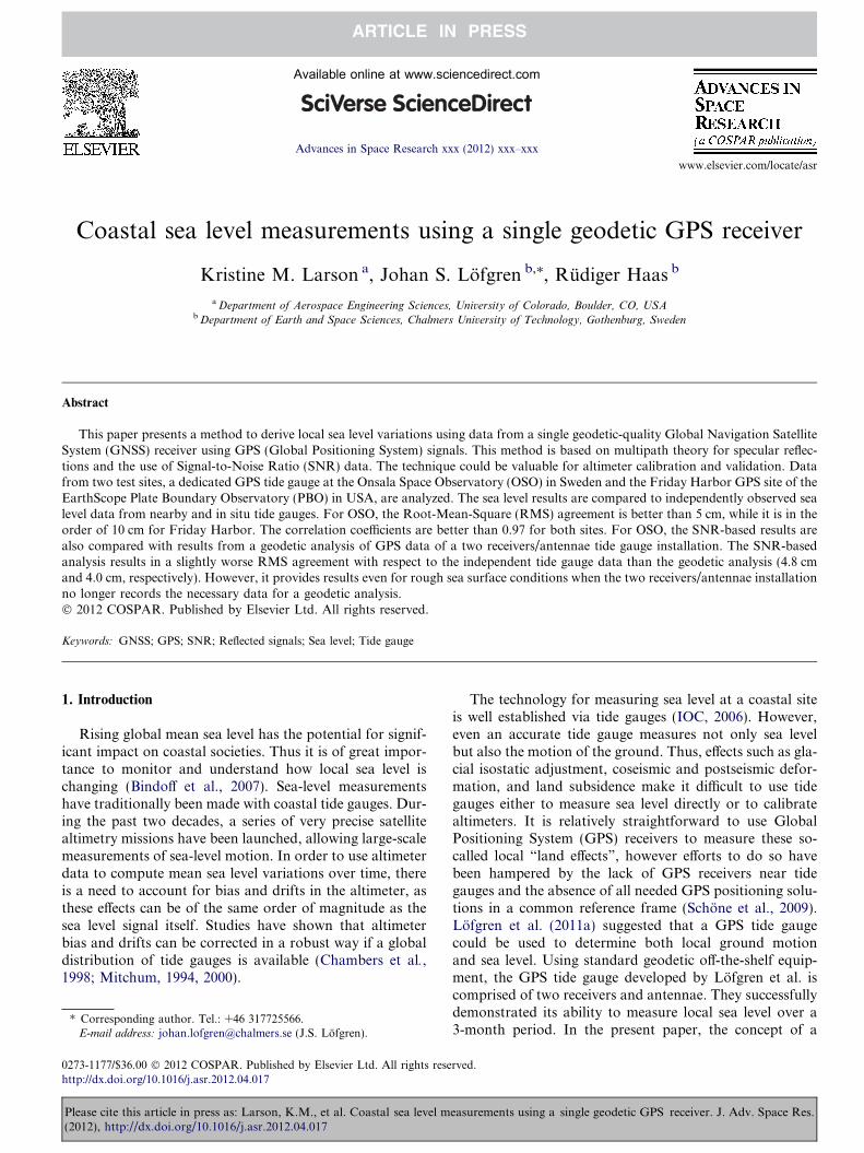
GPS data from Onsala for 2010 (September 16 throughDecember 16) were analyzed. The closest tide gauge recordsfrom the Swedish Meteorological and Hydrological Insti-tute (SMHI) are at Ringhals (18 km south) and Gothenburg(33 km north). For comparison, a synthetic tide gaugerecord was computed (0.4 � Gothenburg and 0.6 � Ringhals)to approximate the sea level record for Onsala. The ratiosused to compute the synthetic tide gauge were based onthe distance of the tide gauges from Onsala. For each satel-lite, a bias was estimated for the three-month period by min-imizing the residual between the GPS sea level heights andthe synthetic tide gauge record. This bias reflects the dis-tance from the GPS phase center to mean sea level asdefined by the SMHI. A total of 24 satellite tracks are visi-ble each day at OSO for the azimuth range used. The GPSand synthetic tide gauge records are shown in Fig. 6. TheGPS results clearly follow the general signature of the tidalvariations over the three-month period. There is no appar-ent drift in the GPS tide gauge records. The standard devi-ation of the residual between the GPS tide gauge and thesynthetic tide gauge is 4.8 cm. The correlation between thesynthetic tide gauge and the GPS tide gauge is shown inFig. 7; the correlation coefficient is 0.97.

3.3. Friday Harbor, WA

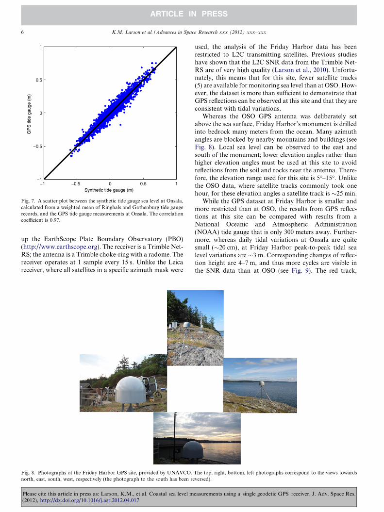
The Friday Harbor GPS tide gauge (Fig. 8) is located�130 km northwest of Seattle, Washington (U.S.). UnlikeOSO, the Friday Harbor site was never meant to be usedto measure ocean reflections. Friday Harbor was installedfor tectonic studies, one of the 1100 GPS receivers that make

310 320 330 340 350ear (2010)

ted from a weighted mean of tide gauge observations at Ringhals andauge (red dots). (For interpretation of the references to colour in this figure



−1 −0.5 0 0.5 1−1

−0.5

0

0.5

1

Synthetic tide gauge (m)

GP

S ti

de g

auge

(m

)

Fig. 7. A scatter plot between the synthetic tide gauge sea level at Onsala,calculated from a weighted mean of Ringhals and Gothenburg tide gaugerecords, and the GPS tide gauge measurements at Onsala. The correlationcoefficient is 0.97.


up the EarthScope Plate Boundary Observatory (PBO)(http://www.earthscope.org). The receiver is a Trimble Net-RS; the antenna is a Trimble choke-ring with a radome. Thereceiver operates at 1 sample every 15 s. Unlike the Leicareceiver, where all satellites in a specific azimuth mask were

Fig. 8. Photographs of the Friday Harbor GPS site, provided by UNAVCO.north, east, south, west, respectively (the photograph to the south has been re


used, the analysis of the Friday Harbor data has beenrestricted to L2C transmitting satellites. Previous studieshave shown that the L2C SNR data from the Trimble Net-RS are of very high quality (Larson et al., 2010). Unfortu-nately, this means that for this site, fewer satellite tracks(5) are available for monitoring sea level than at OSO. How-ever, the dataset is more than sufficient to demonstrate thatGPS reflections can be observed at this site and that they areconsistent with tidal variations.

Whereas the OSO GPS antenna was deliberately setabove the sea surface, Friday Harbor’s monument is drilledinto bedrock many meters from the ocean. Many azimuthangles are blocked by nearby mountains and buildings (seeFig. 8). Local sea level can be observed to the east andsouth of the monument; lower elevation angles rather thanhigher elevation angles must be used at this site to avoidreflections from the soil and rocks near the antenna. There-fore, the elevation range used for this site is 5�–15�. Unlikethe OSO data, where satellite tracks commonly took onehour, for these elevation angles a satellite track is �25 min.

While the GPS dataset at Friday Harbor is smaller andmore restricted than at OSO, the results from GPS reflec-tions at this site can be compared with results from aNational Oceanic and Atmospheric Administration(NOAA) tide gauge that is only 300 meters away. Further-more, whereas daily tidal variations at Onsala are quitesmall (�20 cm), at Friday Harbor peak-to-peak tidal sealevel variations are �3 m. Corresponding changes of reflec-tion height are 4–7 m, and thus more cycles are visible inthe SNR data than at OSO (see Fig. 9). The red track,

The top, right, bottom, left photographs correspond to the views towardsversed).


http://www.earthscope.org


0 5 10 15 20−0.5

0

0.5

1

1.5

2

2.5

3

5o 15o

Time (hr)

Sea

leve

l (m

)

Tide Gauge

Fig. 9. Signal-to-Noise Ratio (SNR) variations for GPS satellites withPseudo-Random Noise (PRN) numbers 17 (red), 7 (magenta), and 31(rising is cyan and setting is blue) for elevation angles of 5�–15� from theFriday Harbor GPS site. Before plotting, the effects of the direct signalwere removed from the SNR data with a 2nd order polynomial. The SNRdata are superimposed on the NOAA tide gauge record for Friday Harborat the time the satellite was rising/setting over the harbor (shown by thecircles). The x-axis for each SNR time series has been exaggerated to makeit easier to see the multipath oscillations in the data; each satellite trackactually extends only �25 min. (For interpretation of the references tocolour in this figure legend, the reader is referred to the web version of thisarticle.)

0 2 4 6 8 10 120

5

10

15

20

25

30

Reflector height (m)

Spe

ctra

l am

plitu

de (

volts

)

PRN 7PRN 31 risePRN 31 setPRN 17

Fig. 10. Lomb Scargle Periodograms for the data shown in Fig. 9.Increases in reflector height correspond to a decrease in sea level.

202 204 206 208 210 212 214 216 218−1

−0.5

0

0.5

1

1.5

2

2.5

Day of year (2011)

Sea

leve

l (m

)

NOAA Tide GaugeGPS

Fig. 11. The Friday Harbor sea level records estimated from GPS (bluedots, 5 per day) and measured by the NOAA (black dashed line) tidegauge. (For interpretation of the references to colour in this figure legend,the reader is referred to the web version of this article.)


the GPS satellite with Pseudo-Random Noise (PRN) code17, corresponds to a reflector height of �4 m and the bluetrack (setting satellite with PRN 31) corresponds to �7 m.Recall, these h values are the distance between the antennaand the sea surface, so that a smaller h value means the seasurface is higher. From Eq. (2), larger values of h meanthat the multipath frequencies are higher, which is consis-tent with what is observed. The LSP results for these fourGPS tracks are shown in Fig. 10. Note that these ampli-tudes of the LSP periodograms are nearly twice as largeas at OSO.


3.4. Friday Harbor tide gauge results

GPS data from Friday Harbor for 2011 (July 5 throughOctober 23) were analyzed. For each satellite, a bias wasestimated for this three-month period by minimizing theresidual between the GPS sea level heights and the NOAAtide gauge data. This bias represents the location of thephase center of the antenna with respect to the tide gaugedatum. Because the tidal variations are so large, a 16-daysubset of the GPS results is shown in Fig. 11 to clearly illus-trate the sea level variations. Although the GPS tide gaugeconvincingly records the overall behavior of the NOAA tidegauge (Fig. 12, correlation of 0.98), the standard deviationof the residual between GPS and the in situ tide gauge is�10 cm. This is much larger than was observed for Onsala.This is due to limitations in the simple model that was usedto estimate the reflector height. Tidal variations at FridayHarbor are on average 20 cm/hour. Each satellite passshown in Fig. 9 takes�25 minutes, and thus the assumptionof a horizontal planar reflector is inadequate. A bettermodel would require estimation of a reflector frequencyand frequency rate; this will be the topic of future work.

4. Discussion

What are the advantages and disadvantages of the twokinds of GPS tide gauges? The dataset of Lofgren et al.(2011b) overlaps with the one used in this study. Againusing a synthetic tide gauge record to simulate sea level vari-ations at Onsala, we can assess the precision of the twomethods. Over the three months of the study, the standarddeviation of the residual between the synthetic tide gaugeand the GPS tide gauge results is 4.0 cm for Lofgren et al.(2011b) if three standard deviation residuals are removed.The RMS is 4.8 cm for the SNR-analysis presented here.



−1 −0.5 0 0.5 1 1.5 2 2.5 3−1

−0.5

0

0.5

1

1.5

2

2.5

3

NOAA tide gauge (m)

GP

S ti

de g

auge

(m

)

Fig. 12. A scatter plot between the sea level results from the NOAA andthe GPS tide gauge at Friday Harbor. The correlation coefficient is 0.98.


We cannot assess the accuracy of either method becauseboth studies eliminated a bias between GPS and the tidegauge record empirically. The SNR-based sea level retrievalpresented here provides a temporal resolution that is deter-mined by the number of satellite arcs, i.e., one sea levelretrieval per satellite arc. On the other hand, the traditionalGPS tide gauge analysis (using two GPS antennae) allows amuch higher temporal resolution (Lofgren et al., 2010).

One advantage of using SNR analysis instead of tradi-tional GPS tide gauge analysis is the superior performanceduring windy conditions. As shown in Fig. 5 of Lofgrenet al. (2011b), the nadir-pointing antenna/receiver system

−0.4

−0.2

0

0.2

0.4

0.6

0.8

Sea

leve

l (m

)

Synthetic TGThis studyLöfgren et al. [2011b]

311 312 313 3140

5

10

15

20

Win

d sp

eed

(m/s

)

Day of y

Fig. 13. Top: the synthetic tide gauge record for Onsala (black line), the GPS tresults by Lofgren et al. (2011b) (yellow dots). Bottom: recorded wind speeds ain this figure legend, the reader is referred to the web version of this article.)


has difficulty tracking the reflected signal when the sea sur-face is rough, corresponding to wind speeds greater than9 m/s. There was little indication of wind speed correlationin the SNR-study presented here, because the receiver wastracking the direct signal, which is not impacted by wind.Fig. 13 shows a one-week period of results for both studies,i.e., from the geodetic analysis of the GPS tide gauge and theSNR analysis. During the first five days, both systems showexcellent sea level retrievals. The nadir-pointing receiver/antenna system then shows very poor tracking for almosttwo days, which correlates with very windy conditions.

Although of less importance, SNR data do not havecycle slips, whereas a geodetic-quality GPS receiver willbe impacted by cycle slips, particularly when it is tryingto track the lower power reflected signals. Since the base-line being determined is extremely small, fixing these cycleslips is not a significant limitation. Of greater importance,the single receiver/antenna system is half the cost of the tra-ditional two receiver/antenna GPS tide gauge. No part ofthe receiver or antenna had to be specially designed orbuilt. These GPS receivers operate with the same trackingloops used by surveyors and geophysicists.

5. Conclusions

The SNR-analysis of three months of GPS data collectedusing geodetic-quality receivers and antennae has demon-strated that such systems are capable of determining sealevel with a precision of �5 cm. This is a degraded perfor-mance relative to the geodetic analysis of the two-antenna/receiver GPS tide gauge system (Lofgren et al.,2011a, b). The primary advantage of any GPS tide gaugeis that it allows simultaneous determination of sea leveland position with respect to the International TerrestrialReference Frame system (e.g. as provided by its latest

315 316 317 318

ear (2010)

ide gauge results presented in this study (red dots), and the GPS tide gauget Onsala Space Observatory. (For interpretation of the references to colour




realization ITRF2008, Altamimi et al., 2011), in this studyeven using a single instrument. This is particularly usefulin areas with land surface motion where the usefulness oftraditional tide gauges is restricted. Because of its simplicity,the cost of the GPS tide gauge described here is half the priceof the two-antenna/receiver GPS tide gauge system. It alsohas better performance in high wind conditions, but pro-vides significantly worse temporal resolution than the two-antenna/receiver system in calm sea surface conditions(30–60 min vs. 5–10 min). Although the number of GPSsites very near the coast is small, as long as the SNR dataare of high quality (Larson et al., 2010), these sites couldbe used as tide gauges. It would be interesting to examineexisting GPS coastal sites to determine if long records couldbe extracted of both ground motion and sea level.

Even though GPS tide gauges are unlikely to replace tra-ditional tide gauges, they might become extremely useful asa campaign instrument for researchers having an interest inmonitoring water levels, even in tectonically active regions.For example, they could be used in altimeter validation/calibration experiments. Because they do not need to belocated in the water, they are simple to install and operateand can be easily moved. For “deliberate” measurementsof water reflections using a geodetic-quality GPS instru-ment, the antenna could be turned to the horizon, thusincreasing the strength of the reflected signals. Extendingthis concept to use satellite signals of other GNSS willimprove the temporal resolution of the geodetic tide gaugeand allow a more comprehensive comparison.

Acknowledgements

K.L.’s work was supported by a 150th Anniversary Vis-iting Professorship at the Chalmers University of Technol-ogy. The U.S. National Science Foundation (NSF)supports reflections research at the University of Colorado:EAR 0948957 and AGS 0935725. Some of the material inthis paper is based on data, equipment, and engineeringservices provided by the Plate Boundary Observatory oper-ated by UNAVCO for EarthScope (http://www.earth-scope.org) and supported by the NSF (EAR-0350028 andEAR-0732947). The GPS data from Friday Harbor shownin this paper are freely available from UNAVCO. TheNOAA tide gauge data (Station 9449880) were down-loaded from http://tidesandcurrents.noaa.gov. The Adler-bert Research Foundation partially funded the GPS tidegauge project at the Onsala Space Observatory. The receiv-ers and antennae were purchased through the Leica Geo-systems ATHENA program. The stilling well tide gaugedata from Ringhals and Gothenburg were provided bythe Swedish Meteorological and Hydrological Institute.

References

Altamimi, Z., Collilieux, X., Metivier, L. ITRF2008, An improvedsolution of the International Terrestrial Reference Frame. J. Geod.85 (8), 457–473, 2011.


Belmonte Rivas, M., Martin-Neira, M. Coherent GPS reflections from thesea surface. IEEE Geosci. Remote Sens. Lett. 3, 28–31, 2006.

Benton, C.J., Mitchell, C.N.. Isolating the multipath component in GNSSsignal-to-noise data and locating reflecting objects. Radio Sci. 46, art.RS6002, http://dx.doi.org/10.1029/2011RS004767, 2011.

Bilich, A., Larson, K.M., Axelrad, P., Modeling GPS phase multipathwith SNR: case study from Salar de Uyuni, Bolivia, J. Geophys. Res.,113, art. B04401, http://dx.doi.org/10.1029/2007JB005194, 2008.

Bindoff, N.L., Willebrand, J., Artale, V., et al. Observations: oceanicclimate change and sea level, in: Solomon, S., Qin, D., Manning, M.,et al. (Eds.), Climate Change 2007: The Physical Science Basis.Contribution of Working Group I to the Fourth Assessment Report ofthe Intergovernmental Panel on Climate Change. Cambridge Univer-sity Press, Cambridge, United Kingdom and New York, NY, USA,2007.

Cardellach, E., Ao, C.O., de la Torre Juarez, M., et al. Carrier phase delayaltimetry with GPS-reflection/occultation interferometry from lowEarth orbiters. Geophys. Res. Lett. 31, art. L10402, http://dx.doi.org/10.1029/2004GL019775, 2004.

Chambers, D., Ries, J.C., Shum, C.K., et al. On the use of tide gauges todetermine altimeter drift. J. Geophys. Res. 103 (C6), 12885–12890,1998.

Dunne, S., Soulat, F., Caparrini, M., et al. OceanPal, A GPS-reflectioncoastal instrument to monitor tide and sea-state. Oceans-Europe 2,1351–1356, 2005.

Elosegui, P., Davis, J.L., Jaldehag, T.K., et al. Geodesy using the GlobalPositioning System: the effects of signal scattering on estimates of siteposition. J. Geophys. Res. 100(B6), 9921–9934, http://dx.doi.org/10.1029/95JB00868, 1995.

Georgiadou, Y., Kleusberg, A. On carrier signal multipath effects inrelative GPS positioning. Manusc. Geod. 13, 172–179, 1988.

Gurtner, W., RINEX: The Receiver-Independent Exchange Format, GPSWorld, 5(7), July 1994.

Hannah, B.M., Modelling and simulation of GPS multipath propagation,Ph.D. thesis, Queensland University of Technology, Brisbane, Aus-tralia, 2001.

IOC (Intergovernmental Oceanographic Commission) of UNESCO.Manual on sea level measurement and interpretation, IV: An updateto 2006, IOC manuals and guides. JCOMM Technical Report No.31,WMO/TD. No.1339, 78 pp., Paris, 2006.

Jaldehag, R.T.K., Johansson, J.M. Ronnang, B.O., et al. Geodesy usingthe Swedish permanent GPS network: effects of signal scattering onestimates of relative site positions. J. Geophys. Res. 101(B8), 17184–17860, http://dx.doi.org/10.1029/96JB01183, 1996.

Joseph, A. What is the difference between SNR and C/N0? InsideGNSS 5(8), 20–25, 2010.

Larson, K.M., Small, E.E. Gutmann, E., et al.. Use of GPS receivers as asoil moisture network for water cycle studies. Geophys. Res. Lett. 35,art. L24405, http://dx.doi.org/10.1029/2008GL036013, 2008.

Larson, K.M., Gutmann, E., Zavorotny, V., et al. Can we measure snowdepth with GPS receivers? Geophys. Res. Lett. 36, art. L17502, http://dx.doi.org/10.1029/2009GL039430, 2009.

Larson, K.M., Braun, J., Small, E.E., et al. GPS multipath and its relationto near-surface soil moisture content. IEEE J-STARS 3, 91–99, http://dx.doi.org/10.1109/JSTARS.2009.2033612, 2010.

Larson, K.M., Nievinski, F. GPS snow sensing: results from theEarthScope Plate Boundary Observatory, GPS Solut. http://dx.doi.org/10.1007/s10291-012-0259-7, 2012.

Lofgren, J.S., Haas, R. Johansson, J.M. High-rate local sea levelmonitoring with a GNSS-based tide gauge, in: Proceedings of the2010 IEEE IGRSS, 25–30 July, Honolulu, HI, USA, pp. 3616–3619,2010.

Lofgren, J.S., Haas, R., Johansson, J.M. Monitoring coastal sea levelusing reflected GNSS signals. Adv. Space Res. 47 (2), 213–220, 2011a.

Lofgren, J., Haas, R., Scherneck, H.-G. et al., Three months of local sealevel derived from reflected GNSS signals. Radio Sci. 46, art. RS0C05,http://dx.doi.org/10.1029/2011RS004693, 2011b.


http://tidesandcurrents.noaa.gov

http://dx.doi.org/10.1029/2011RS004767

http://dx.doi.org/10.1029/2007JB005194

http://dx.doi.org/10.1029/2004GL019775

http://dx.doi.org/10.1029/2004GL019775

http://dx.doi.org/10.1029/95JB00868



http://dx.doi.org/10.1029/2008GL036013

http://dx.doi.org/10.1029/2009GL039430

http://dx.doi.org/10.1029/2009GL039430

http://dx.doi.org/10.1109/JSTARS.2009.2033612

http://dx.doi.org/10.1109/JSTARS.2009.2033612

http://dx.doi.org/10.1007/s10291-012-0259-7

http://dx.doi.org/10.1007/s10291-012-0259-7

http://dx.doi.org/10.1029/2011RS004693



Lowe, S.T., LaBrecque, J.L., Zuffada, C., et al. First spaceborneobservation of an Earth-reflected GPS signal. Radio Sci. 37(1), art.1007, http://dx.doi.org/10.1029/2000RS002539, 2002.

Martin-Neira, M. A passive reflectometry and interferometry system(PARIS): application to ocean altimetry. ESA J. 17, 331–355, 1993.

Martin-Neira, M., Caparrini, M., Font-Rossello, J., et al. The PARISconcept: an experimental demonstration of sea surface altimetry usingreflected GPS signals. IEEE Trans. Geosci. Rem. Sens. 39 (1), 142–150,2001.

Mitchum, G.T. Comparison of Topex sea surface heights and tide gaugesea levels. J. Geophys. Res. 99 (C12), 24541–24554, 1994.

Mitchum, G.T. An improved calibration of satellite altimetric heightsusing tide gauge sea levels with adjustment for land motion. Mar.Geod. 23, 145–166, 2000.

Park, K.-D., Elosegui, P., Davis, J.L., et al. Development of an antennaand multipath calibration system for Global Positioning System sites.


Radio Sci., 39, art. RS5002, http://dx.doi.org/10.1029/2003RS002999,2004.

Press, F., Teukolsky, S., Vetterling, W., et al. Numerical Recipes inFortran 90: The art of parallel scientific computing, second ed.Cambridge University Press, 1996.

Rius, A., Nogues-Correig, O., Ribo, S, et al. Altimetry with GNSS-Rinterferometry: first proof of concept experiment, GPS Sol., http://dx.doi.org/10.1007/s10291-011-0225-9, in press.

Schone, T., Schon, N., Thaller, D. IGS tide gauge benchmark monitoringpilot project (TIGA), Scientific benefits. J. Geod. 83 (3–4), 249–261,2009.

Soulat, F., Caparrini, M., Germain, O., et al., Sea state monitoring usingcoastal GNSS-R, Geophys. Res. Lett. 31, art. L21303, http://dx.doi.org/10.1029/2004GL020680, 2004.

Treuhaft, R., Lowe, S., Zuffada, C., et al. 2-cm GPS altimetry over CraterLake. Geophys. Res. Lett. 22 (23), 4343–4346, 2001.


http://dx.doi.org/10.1029/2000RS002539

http://dx.doi.org/10.1029/2003RS002999

http://dx.doi.org/10.1007/s10291-011-0225-9

http://dx.doi.org/10.1007/s10291-011-0225-9

http://dx.doi.org/10.1029/2004GL020680

http://dx.doi.org/10.1029/2004GL020680


coastal sea level measurements using a single geodetic gps

Documents