ERD

C/CH

L TR

-14-

2

Coastal Inlets Research Program

Coastal Modeling System Mathematical Formulations and Numerical Methods

Coas

tal a

nd H

ydra

ulic

s La

bora

tory

Alejandro Sánchez, Weiming Wu, Honghai Li, Mitch Brown, Chris Reed, Julie Rosati, and Zeki Demirbilek

March 2014

Approved for public release; distribution is unlimited.

The US Army Engineer Research and Development Center (ERDC) solves the nation’s toughest engineering and environmental challenges. ERDC develops innovative solutions in civil and military engineering, geospatial sciences, water resources, and environmental sciences for the Army, the Department of Defense, civilian agencies, and our nation’s public good. Find out more at www.erdc.usace.army.mil.

To search for other technical reports published by ERDC, visit the ERDC online library at http://acwc.sdp.sirsi.net/client/default.

Coastal Inlets Research Program ERDC/CHL TR-14-2 March 2014

Coastal Modeling System Mathematical Formulations and Numerical Methods

Alejandro Sánchez, Honghai Li, Mitch Brown, Julie Rosati, and Zeki Demirbilek Coastal and Hydraulics Laboratory US Army Engineer Research and Development Center 3909 Halls Ferry Road, Vicksburg, MS 39180-6199

Weiming Wu National Center for Computational Hydroscience and Engineering The University of Mississippi 327 Brevard Hall, University Road Oxford, MS 38677

Christopher Reed Reed & Reed Consulting 1400 Village Square Blvd Ste 3-146 Tallahassee, FL 32312-3909

Final report Approved for public release; distribution is unlimited.

ERDC/CHL TR-14-2 ii

Abstract

The Coastal Modeling System (CMS) is an integrated numerical modeling system for simulating nearshore waves, currents, water levels, salinity and sediment transport, and morphology change. The CMS was designed and developed for coastal inlets and navigation applications, including channel performance and sediment exchange between inlets and adjacent beaches. The present report provides an updated description of the mathematical formulations and numerical methods of hydrodynamic, salinity and sediment transport, and morphology change model CMS-Flow. The CMS-Flow uses the Finite Volume Method on Cartesian grids and has both fully explicit and fully implicit time-stepping schemes. A detailed description of the explicit time-stepping scheme was provided in Militello et al. (2004) and Buttolph et al. (2006). The present report focuses on the recent changes in the mathematical formulations and the implicit time-stepping schemes. The CMS-Wave and CMS-Flow models are tightly coupled within a single inline code. The CMS-Wave and CMS-Flow grids may be the same or have different spatial extents and resolutions. The hydrodynamic model includes physical processes such as advection, turbulent mixing, combined wave-current bottom friction; wave mass flux; wind, atmospheric pressure, wave, river, and tidal forcing; Coriolis force; and the influence of coastal structures. The implicit hydrodynamic model is coupled to a nonequilibrium transport model of multiple-sized total-load sediments. The model includes physical processes such as hiding and exposure, bed sorting and gradation, bed slope effects, nonerodible surfaces, and avalanching.

DISCLAIMER: The contents of this report are not to be used for advertising, publication, or promotional purposes. Citation of trade names does not constitute an official endorsement or approval of the use of such commercial products. All product names and trademarks cited are the property of their respective owners. The findings of this report are not to be construed as an official Department of the Army position unless so designated by other authorized documents. DESTROY THIS REPORT WHEN NO LONGER NEEDED. DO NOT RETURN IT TO THE ORIGINATOR.

ERDC/CHL TR-14-2 iii

Contents Abstract .......................................................................................................................................................... ii

Figures and Tables ......................................................................................................................................... v

Preface ............................................................................................................................................................ vi

List of Symbols ........................................................................................................................................... viii

Unit Conversion Factors ............................................................................................................................xiv

1 Introduction ............................................................................................................................................ 1

2 Mathematical Formulations ............................................................................................................... 5 Coordinate System ................................................................................................................... 5 Hydrodynamics ......................................................................................................................... 5

Variable Definitions ...................................................................................................................... 5 Governing Equations .................................................................................................................... 7 Bed Shear Stresses ...................................................................................................................... 8 Bottom Wave Orbital Velocity .................................................................................................... 12 Eddy Viscosity ............................................................................................................................. 14 Wave Radiation Stresses ........................................................................................................... 17 Roller Stresses ........................................................................................................................... 18 Wave Flux Velocity ...................................................................................................................... 18 Wind Surface Stress ................................................................................................................... 19 Boundary Conditions .................................................................................................................. 21

Salinity Transport.................................................................................................................... 26 Overview ..................................................................................................................................... 26 Transport Equation .................................................................................................................... 26 Initial Condition .......................................................................................................................... 27 Boundary Conditions .................................................................................................................. 27

Sediment Transport ................................................................................................................ 27 Overview ..................................................................................................................................... 27 Non-equilibrium Total-Load Transport Model ........................................................................... 28 Bed Material Sorting and Layering ........................................................................................... 35 Sediment Fall Velocity ................................................................................................................ 36 Equilibrium Concentrations and Transport Rates .................................................................... 37 Hiding and Exposure .................................................................................................................. 44 Incipient Motion ......................................................................................................................... 46 Ripple Dimensions ..................................................................................................................... 47 Horizontal Sediment Mixing Coefficient .................................................................................... 49 Boundary Conditions .................................................................................................................. 49

3 Numerical Methods ............................................................................................................................ 50 Overview ................................................................................................................................. 50

ERDC/CHL TR-14-2 iv

Computational Grid ................................................................................................................ 50 General Transport Equation ................................................................................................... 54

Spatial Discretization ................................................................................................................. 54 Temporal Discretization ............................................................................................................. 55 Cell-face Interpolation ................................................................................................................ 56 Cell-face Gradient ....................................................................................................................... 57 Cell-centered Gradient ............................................................................................................... 57 Reconstruction, Monotonicity, and Slope Limiters .................................................................. 57 Advection Schemes .................................................................................................................... 60 Source/Sink Term ...................................................................................................................... 61 Assembly of Algebraic Equations .............................................................................................. 61 Implicit Relaxation ...................................................................................................................... 61 Iterative Solvers .......................................................................................................................... 62 Convergence and Time-Stepping .............................................................................................. 63 Ramp Function ........................................................................................................................... 65

Hydrodynamics ....................................................................................................................... 66 Coupling of Velocity and Water Level – SIMPLEC Algorithm ................................................... 66 Wetting and Drying ..................................................................................................................... 68

Salinity Transport.................................................................................................................... 68 Transport Equation .................................................................................................................... 68 Laplace Equation ....................................................................................................................... 68

Sediment Transport and Morphology Change ...................................................................... 68 Transport Equations ................................................................................................................... 69 Bed Change Equations .............................................................................................................. 69 Bed Material Sorting .................................................................................................................. 70 Avalanching ................................................................................................................................ 70 Hard bottom ............................................................................................................................... 72 Coupling of Sediment Transport, Bed Change, and Sorting Equations .................................. 72

Coupling Procedure of CMS-Flow and CMS-Wave ................................................................ 73 Spatial Interpolation and Extrapolation .................................................................................... 75 Temporal Interpolation and Prediction ..................................................................................... 76

4 Summary ............................................................................................................................................... 78

References ................................................................................................................................................... 80

Report Documentation Page

ERDC/CHL TR-14-2 v

Figures and Tables

Figures

Figure 1-1. CMS framework and its components. ..................................................................................... 2 Figure 2-1. Vertical conventions used for the bed and mean water surface elevation. ....................... 5 Figure 2-2. Modified Hsu (1988) wind drag coefficient. ......................................................................... 20 Figure 2-3. Schematic of sediment and current vertical profiles. ......................................................... 32 Figure 2-4. Suspend load correction factors based on the logarithmic velocity profile and (a) exponential and (b) Rouse suspended sediment profile. ....................................................... 33 Figure 2-5. Multiple bed layer model of bed material sorting (after Wu 2007). .................................. 36 Figure 2-6. Schematic of the exposure height of bed sediment grains. ............................................... 45 Figure 3-1. Examples of invalid Cartesian computational grids. ........................................................... 51 Figure 3-2. Types of Cartesian grids supported by the SMS interface and CMS-Flow........................ 52 Figure 3-3. Computational stencils and control volumes for two types of Cartesian grids: non-uniform Cartesian (left) and telescoping grid (right). ....................................................................... 53 Figure 3-4. Schematic showing interface interpolation: (a) coarse to fine and (b) fine to coarse. ........................................................................................................................................................... 56 Figure 3-5. Schematics showing examples of (a) non-limited and (b) limited linear reconstructions. ............................................................................................................................................ 58 Figure 3-6. Comparison of three different slope limiters. ....................................................................... 59 Figure 3-7. Ramp function used in CMS. .................................................................................................. 65 Figure 3-8. Schematic showing an example bed layer evolution. Colors indicate layer number and not bed composition. ............................................................................................................ 71 Figure 3-9. Coupling process between CMS-Flow and CMS-Wave. ....................................................... 73 Figure 3-10. Schematic of steering process. ............................................................................................ 74

Tables

Table 2-1. Fitting coefficients for combined wave-current mean bottom friction. ............................... 12 Table 2-2. Tidal constituents implemented in CMS. Constituent speeds are in degrees per mean solar hour. .......................................................................................................................................... 24 Table 3-1. Default criteria to determine whether the iterative solution procedure has converged, diverged, or requires a reduced time-step. .......................................................................... 64

ERDC/CHL TR-14-2 vi

Preface

This report was written by the Coastal Inlets Research Program (CIRP) and funded by the US Army Corps of Engineers, Headquarters (HQUSACE). The CIRP is administered at the US Army Engineer Research and Development Center (ERDC), Coastal and Hydraulics Laboratory (CHL) under the Navigation R&D Program. Jeff E. Mckee was HQUSACE Navigation Business Line Manager overseeing CIRP. Jeff Lillycrop, CHL, was the Technical Director of the Navigation R&D Program. Dr. Julie Rosati, CHL, was the CIRP Program Manager.

CIRP conducts applied research to improve USACE capabilities to manage federally-maintained inlets and navigation channels, which are present on all coasts of the United States, including the Atlantic Ocean, Gulf of Mexico, Pacific Ocean, Great Lakes, and US territories. The objectives of CIRP are to advance knowledge and provide quantitative, predictive tools to accomplish the following: (a) support management of federal coastal inlet navigation projects — principally the design, maintenance, and operation of channels and jetties, and reduce the cost of dredging; and (b) preserve the adjacent beaches and estuary in a systems approach that treats the inlet, beaches, and estuary as sediment-sharing components. To achieve these objectives, CIRP is organized in work units conducting research and development in computational modeling, laboratory and field investigations, and technology transfer.

For the mission-specific requirements, CIRP has developed a finite-volume model based on nonlinear shallow-water flow equations, called CMS-Flow, specifically for inlets, navigation, and nearshore project applications. The governing equations are solved using both explicit and implicit Finite Volume Method on Cartesian coordinates. The model is part of the Coastal Modeling System (CMS) intended to simulate nearshore waves, flow, sediment transport, and morphology change affecting planning, design, maintenance, and reliability of federal navigation projects.

The work described in the report was performed under the Harbors Entrances and Structures Branch of the Navigation Division, US Army Engineer Research and Development Center, Coastal and Hydraulics

ERDC/CHL TR-14-2 vii

Laboratory (ERDC-CHL). At the time of publication, Dr. Donald Ward was Acting Branch Chief; Dr. Jackie Pettway was Division Chief; Jeff Lillycrop was Technical Director; Dr. Richard Styles was Deputy Director; and José Sánchez was the Laboratory Director.

COL Jeffrey R. Eckstein was ERDC Commander. Dr. Jeffery Holland was ERDC Director.

ERDC/CHL TR-14-2 viii

List of Symbols

Symbol Description Units

wA Wave bottom semi-orbital excursion m

cRA Empirical coefficient in the Lund-CIRP transport formula

WatA Empirical coefficient for the Watanabe sediment transport formula

c Wave celerity m/s

bc Bed friction coefficient -

brc Wave breaking coefficient for eddy viscosity -

Dc Wind drag coefficient -

gc Wave groups velocity m/s

hc Horizontal shear coefficient -

Rc References near-bed sediment concentration for the Lund-CIRP transport formula

-

wc Empirical coefficient for wave bottom friction -

wfc Wave bottom friction coefficient for eddy viscosity -

vc Vertical shear coefficient -

salC Depth-averaged salinity psu or ppt

*tkC Fractional equilibrium depth-averaged total-load

concentration **tk k tkC p C 1

kg/m3

*tkC

Potential fractional equilibrium depth-averaged total-load concentration

kg/m3

d Grain size m

*d Dimensionless grain size -

50d Sediment grain size in meters of 50th percentile m

90d Sediment grain size in meters of 90th percentile m

eD Total effective dissipation N/m/s

brD Wave breaking dissipation N/m/s

ERDC/CHL TR-14-2 ix

sD Bed slope coefficient for sediment transport

ije Deformation (strain rate) tensor 1/s

srE Surface roller energy density N/m

wE Wave energy 2116 sgHρ= N/m

η Instantaneous water level m

tη Instantaneous wave trough elevation m

f Wave frequency 1/s

bf Bed-load scaling factor -

cf Coriolis parameter 1/s

sf Suspended-load scaling factor -

morphf Morphologic acceleration factor -

Rampf Ramp function -

f⊥ Linear interpolation factor used to calculate cell face variables

-

wf Wave friction factor. -

g Gravitational constant ~9.81 m/s2 m/s2

h Total wave-averaged water depth m

H Wave height m

rmsH Root-mean-squared wave height m

rH Ripple height m

sH Significant wave height m

k Wave number rad/m

sk Nikuradse roughness m

srk Form-drag (ripple) roughness

sgk Grain-related roughness

hl Mixing length m

rL Ripple length m

ERDC/CHL TR-14-2 x

bm Bed slope coefficient for momentum equations -

n Manning’s roughness coefficient s/m1/3

n′ Grain-related Manning’s roughness coefficient 1/650 / 20d=

p Water level pressure gρ η= Pa

ap Atmospheric pressure Pa

ekP Total probability of exposure for the kth sediment size class

-

fP Peclet number calculated at the cell face -

hkP Total probability of hiding for the kth sediment size class -

mp′ Bed porosity -

1kp Fraction of the kth sediment size class in the first layer

*bq

Potential equilibrium bed-load transport rate kg/m/s

*tq

Potential total-load transport rate kg/m/s

*sq

Potential suspended-load transport rate kg/m/s

sr Fraction of suspended load of the total load -

ijR Surface roller stress Pa m

mR Normalized residual error

s Sediment specific gravity -

mS Source term due to precipitation, evaporation, and structures in the momentum equation

m/s

ijS Wave radiation stress Pa m

uS Wave orbital velocity spectrum density s m2/s2

t Time s

Rampt Ramp duration

T Wave period s

pT Peak wave period s

zT Zero-crossing wave period s

nT /h g= s

ERDC/CHL TR-14-2 xi

iu Wave (oscillatory) velocity m/s

iu′ Turbulent velocity fluctuation m/s

U Current magnitude m/s

crU Critical depth-averaged velocity for incipient motion for combined waves and currents

crcU Critical depth-averaged velocity for initiation of motion for currents

m/s

crwu Critical bottom wave orbital velocity amplitude for waves alone

m/s

eU Effective velocity used for sediment transport m/s

wiU Depth-averaged wave flux velocity m/s

wsu Bottom wave orbital velocity magnitude based on the significant wave height and peak wave period using linear wave theory

m/s

rmsu Root-mean-squared bottom wave orbital velocity amplitude

m/s

bu Instantaneous bottom orbital velocity m/s

*u Bed shear velocity /bτ ρ= m/s

iV Total flux velocity or simply total flux velocity m/s

fV Outward cell face total flux velocity m/s

iw Wave unit vector (cos ,sin )θ θ= -

iW Wind velocity at 10-m height m/s

( , , )ix x x y z= =

Cartesian coordinates m

y′ Distance to the nearest wall m

0z Bed roughness length

bz Bed elevation m

aα Under-relaxation parameter for avalanching -

φα Under-relaxation parameter for φ -

tα Total-load adaptation coefficient -

cβ Weighting factor / ( )wU U u= +

∇ Gradient operator 1/m

ERDC/CHL TR-14-2 xii

maxδ Maximum bed layer thickness m

minδ Minimum bed layer thickness m

∆ Average grid size m

A∆ Cell area m2

l∆ Cell face length m

ε Vertical sediment diffusivity m2/s

Γ Diffusion coefficient for φ m2/s

κ Von Karman constant (=0.4) -

wcλ Nonlinear bottom friction enhancement factor -

0ν Base value for the total eddy viscosity m2/s

ν Kinematic viscosity m2/s

cν Current-related component of the total eddy viscosity m2/s

wν Wave-related component of the total eddy viscosity m2/s

tν Total eddy viscosity m2/s

sω Sediment fall velocity s

φ General scalar

Φ Slope limiter -

wψ Wave mobility parameter -

ρ Water density kg/m3

aρ Air density at sea level [~1.2 kg/m3] kg/m3

sρ Sediment (solid or material) density kg/m3

cσ Current -related Schmidt number -

sσ Schmidt number for sediment transport -

salσ Schmidt number for salinity transport -

wσ Wave -related Schmidt number -

siτ Wind surface stress Pa

biτ Combined wave and current mean bed shear stress

maxbτ Maximum bed shear stress under waves and currents Pa

ERDC/CHL TR-14-2 xiii

θ Wave direction (going to) rad

cΘ Shields parameters due to currents -

,cw mΘ

Maximum Shields parameters due to waves and currents -

crΘ Critical Shields parameter -

kξ Hiding and exposure coefficient -

ERDC/CHL TR-14-2 xiv

Unit Conversion Factors

Multiply By To Obtain

cubic yards 0.7645549 cubic meters

degrees (angle) 0.01745329 radians

feet 0.3048 meters

knots 0.5144444 meters per second

miles (nautical) 1,852 meters

miles (US statute) 1,609.347 meters

miles per hour 0.44704 meters per second

pounds (force) 4.448222 Newtons

pounds (force) per foot 14.59390 Newtons per meter

pounds (force) per square foot 47.88026 Pascals

square feet 0.09290304 square meters

square miles 2.589998 E+06 square meters

tons (force) 8,896.443 Newtons

tons (force) per square foot 95.76052 kilopascals

yards 0.9144 meters

ERDC/CHL TR-14-2 1

1 Introduction

The Coastal Modeling System (CMS) is a numerical modeling system for nearshore waves, currents, water levels, sediment transport, and morphology change (Militello et al. 2004; Buttolph et al. 2006; Lin et al. 2008; Reed et al. 2011). The system was developed and continues to be supported by the Coastal Inlets Research Program (CIRP), a research and development program of the US Army Corps of Engineers (USACE) that is funded by the Operation and Maintenance Navigation Business Line of the USACE. The CMS is designed for coastal inlets and navigation applications including channel performance and sediment exchange between inlets and adjacent beaches. Modeling provides planners and engineers with essential information for reducing costs of USACE Operation and Maintenance activities. CIRP is developing, testing, improving, and transferring the CMS to Corps Districts and industry and assisting users with engineering studies.

The overall framework of the CMS and its components are presented in Figure 1-1. The CMS includes a flow model (CMS-Flow) that calculates hydrodynamics, salinity and sediment transport, and morphology change and a spectral wave transformation model (CMS-Wave). The CMS-Wave and CMS-Flow models are tightly coupled within a single inline code and may have the same or different computational grids. CMS takes advantage of the Surface-water Modeling System (SMS) interface versions 8.1 and newer (Militello et al. 2004; Zundel 2006). The SMS is used for grid generation, model setup, generating input files, plotting and post-processing of results. The SMS may be used to extract boundary condi-tions from a larger-domain simulation (Buttolph et al. 2006). The SMS also provides a link between the CMS and the Lagrangian Particle Tracking Model (PTM) (MacDonald et al. 2006; Li et al. 2011).

CMS-Wave is a spectral wave transformation model and solves the wave-action balance equation using a forward marching Finite Difference Method (Mase et al. 2005; Lin et al. 2008; Lin et al. 2011a; Lin et al. 2012). CMS-Wave includes physical processes such as wave shoaling, refraction, diffraction, reflection, wave-current interaction, wave breaking, wind wave generation, white capping of waves, and the influence of coastal structures on waves.

ERDC/CHL TR-14-2 2

Figure 1-1. CMS framework and its components.

CMS-Flow is a two-dimensional horizontal (2DH) depth-integrated and wave-averaged nearshore hydrodynamic, salinity and sediment transport, and morphology change model. CMS-Flow calculates currents and water levels, including physical processes such as advection, turbulent mixing, combined wave-current bottom friction; wave mass flux; wind, atmospheric pressure, wave, river, and tidal forcing; Coriolis force; and the influence of coastal structures (Buttolph et al. 2006; Wu et al. 2011).

CMS-Flow has three noncohesive sediment transport models which differ mainly in the assumption of the local equilibrium transport for the bed and suspended loads (Buttolph et al. 2006; Sánchez and Wu 2011a,b). CMS-Flow can simulate any number of sediment size fractions, the interactions between size fractions, bed sorting and layering, and morphology change. The sediment transport model also includes processes such as avalanching, nonerodible surfaces, and bed slope effects.

Typical applications of CMS-Flow include analyses of past and future navigation channel performance; wave, current, and wave-current interaction in channels and in the vicinity of navigation structures; and sediment management issues around coastal inlets and adjacent beaches.

ERDC/CHL TR-14-2 3

Some examples of CMS-Flow applications are as follows: Batten and Kraus (2006), Buttolph et al. (2006), Zarillo and Brehin (2007), Li et al. (2009), Beck and Kraus (2010), Byrnes et al. (2010), Dabees and Moore (2011), Reed and Lin (2011), Rosati et al. (2011), Wang and Beck (2011), Beck and Legault (2012), and Lin et al. (2013).

A detailed description of the theory and numerical methods for CMS was provided in Militello et al. (2004) and Buttolph et al. (2006). Lin et al. (2008) provided a description of the mathematical formulation and verification and validation cases for the spectral wave model CMS-Wave. More recently, several verification and validation tests were presented for waves (Lin et al. 2011b), hydrodynamics (Sánchez et al. 2011a), and sediment transport and morphology change (Sánchez et al. 2011b). User guidance on how to setup, run, calibrate, and analyze results for the CMS was presented in Lin et al. (2011b) and Sánchez et al. (2011a,b). Since the publication of Buttolph et al. (2006), there have been several changes and added features and processes in the hydrodynamic and sediment transport models. The purpose of the present report is to provide an updated description of the mathematical formulation and numerical methods with focus on the aspects which have recently changed. In particular, this report focuses on the implicit temporal solution scheme for hydrodynamics, sediment, and salinity transport. The explicit temporal solution scheme is described in detail in Buttolph et al. (2006). Currently, the explicit and implicit versions of the CMS-Flow are being merged into a single code. Once this task is completed, another verification and validation study will be conducted with comparisons between the two temporal schemes using the previous and new test cases.

To put both the purpose and contents of this report in perspective, it is necessary to emphasize that this report is not a self-standing, all-inclusive document about the implicit CMS-Flow model. This report must be employed together with the User’s Guide and reports published for the explicit flow model. The User’s Guide is in preparation and will provide users detailed information about model input parameters and coefficients which appear in this report. The User’s Guide also provides guidance on choice of methods, formulas, scaling factors, etc. Last, it is noted that CMS solves a depth-averaged salinity transport equation but does not include an equation of state to calculate the spatially and temporally variable water density. These cautions are provided here to help users understand model

ERDC/CHL TR-14-2 4

limitations, sources of information needed for model input, and proper application of the model.

The report is organized as follows: Chapter 2 presents the governing equations, parameterizations, empirical equations, boundary and initial conditions for hydrodynamics, salinity and sediment transport, and morphology change. Variable definitions with units are also provided. Chapter 3 presents the numerical methods. The Finite Volume discretization is presented for a general transport equation in order to avoid redundancy. The fully implicit iterative solvers for hydrodynamics and total-load sediment transport are described in detail. Chapter 4 is the summary, and Chapter 5 contains the references.

ERDC/CHL TR-14-2 5

2 Mathematical Formulations

Coordinate System

Before presenting the depth-integrated and wave-averaged governing equations, it is useful to define the coordinate system and basic variables. Variables are defined spatially in a Cartesian coordinate system

( , , )ix x x y z

, where x and y are the horizontal coordinates, and z is

the vertical coordinate (positive is upwards). A schematic of several of the main variables in the vertical direction is provided in Figure 2-1. The vertical coordinate datum is usually the Still Water Level (SWL). The bed elevation ( bz ) is measured from the vertical datum (i.e., negative

downwards).

Figure 2-1. Vertical conventions used for the bed and mean water surface elevation.

Hydrodynamics

This section provides a detailed description of the depth-integrated and wave-averaged hydrodynamic equations. The equations described here closely follow those presented in Phillips (1977), Mei (1983), and Svendsen (2006). Variable definitions and the final hydrodynamic equations are provided here. Detailed derivations may be obtained from the preceding references.

Variable Definitions

The instantaneous current velocity ( iu ) is split into

Datum

ζh

η

h η ζ= +

Bed

Mean Water Surface Elevation

bzbzζ = −

ERDC/CHL TR-14-2 6

i i i iu u u u (2-1)

in which

iu = current (wave-averaged) velocity [m/s]

iu = wave (oscillatory) velocity [m/s] with wave-average iu = 0

below the wave trough iu′ = turbulent velocity fluctuation [m/s] with ensemble average

iu′ = 0, and wave average iu′ = 0.

The wave-averaged total volume flux is defined as

b

η

i izhV u dz (2-2)

where:

h = wave-averaged total water depth bh zη= − (Figure 2-1) [m] iV = total mean mass flux velocity, or simply total flux velocity

[m/s] η = instantaneous water level with respect to the Still Water Level

(SWL) [m] η = wave-averaged water surface elevation with respect to the SWL

(Figure 2-1) [m] bz = bed elevation with respect to the SWL (Figure 2-1) [m].

The total flux velocity is also referred to as the mean transport velocity (Phillips 1977) and mass transport velocity (Mei 1983). The current volume flux is defined as

b

η

i izhU u dz (2-3)

where iU is the depth-averaged current velocity. Similarly, the wave

volume flux is defined as

t

η

wi wi iηQ hU u dz (2-4)

ERDC/CHL TR-14-2 7

where:

wiU = depth-averaged wave flux velocity [m/s] tη = instantaneous wave trough elevation [m] .

Therefore, the total flux velocity can be written as

i i wiV U U . (2-5)

Governing Equations

On the basis of the above definitions, and assuming depth-uniform currents, the general depth-integrated and wave-averaged continuity and momentum equations can be written as (Phillips 1977; Svendsen 2006)

( )j m

j

hVh St x

(2-6)

( )( ) j ii aij c j

j i i

i si bit ij ij wi wj b

j j j

hV VhV pη hε f hV ght x x ρ x

V τ τν h S R ρhU U m

x x ρ x ρ ρ

1 (2-7)

where:

t = time [s] jx = horizontal Cartesian coordinate in the jth direction [m], j=1, 2

or x, y mS = source term due to precipitation, evaporation and structures

(e.g., culverts) [m/s] cf = 2 sinφΩ = Coriolis parameter [rad/s] in which Ω= 7.29×10-5

rad/s is the Earth’s angular velocity of rotation, and φ is the latitude in degrees

g = gravitational constant (~9.81 m/s2) ap = atmospheric pressure [Pa] ρ = water density (~1025 kg/m3) tν = total eddy viscosity [m2/s] siτ = wind surface stress [Pa]

ERDC/CHL TR-14-2 8

ijS = wave radiation stress [Pa]

ijR = surface roller stress [Pa]

bm = bed slope coefficient [-] biτ = combined wave and current mean bed shear stress [Pa].

The above 2DH equations are similar to those derived by Svendsen (2006), except for the inclusion of the water source/sink term in the continuity equation and the atmospheric pressure and surface roller terms and the bed slope coefficient in the momentum equation. It’s also noted that the horizontal mixing term is formulated slightly differently as a function of the total flux velocity, similar to the Generalized Lagrangian Mean (GLM) approach (Andrews and McIntyre 1978; Walstra et al. 2000). This approach is arguably more physically meaningful and also simplifies the discretization in the case where the total flux velocity is used as the model prognostic variable.

Bed Shear Stresses

Bed Roughness

The bed roughness is specified for the hydrodynamic calculations with either a Manning's roughness coefficient ( n ), Nikuradse roughness height ( sk ), or bed friction coefficient ( bc ). It is important to note that the bed

roughness is assumed constant in time and not changed according to bed composition and bedforms. This is a common engineering approach which can be justified by the lack of data to initialize the bed composition and the large error in estimating the bed composition evolution and bedforms. In addition using a constant bottom roughness simplifies the model calibra-tion. In future versions of CMS, the option to automatically estimate the bed roughness from the bed composition and bedforms will be added. In addition, the bed roughness used for hydrodynamics may not be the same as that which is used for the sediment transport calculations because each sediment transport formula was developed and calibrated using specific methods for estimating bed shear stresses or velocities, and these cannot be easily changed.

The bed friction coefficient ( bc ) is related to the Manning’s roughness

coefficient ( n ) by (Soulsby 1997)

/bc gn h 2 1 3 (2-8)

ERDC/CHL TR-14-2 9

Commonly, the bed friction coefficient is calculated by assuming a logarithmic velocity profile as (Graf and Altinakar 1998)

ln( / )b

κcz h

2

0 1 (2-9)

where κ =0.4 is Von Karman constant, and 0z is the bed roughness length

which is related to the Nikuradse roughness ( sk ) by 0 / 30sz k=

(hydraulically rough flow).

Current-Related Shear Stress

The current bed shear stress is given by

ci b iτ ρc UU (2-10)

where:

ρ = water density (~1025 kg/m3) bc = bed friction coefficient [-]

U i iU U= = current magnitude [m/s].

The magnitude of the current-related bed shear stress is simply

c bτ ρc U 2 (2-11)

Wave-Related Bed Shear Stress

The wave-related bed shear stress amplitude is given by (Jonsson 1966)

w w wτ ρf u 212

(2-12)

where wf is the wave friction factor, and wu is an equivalent or representa-

tive bottom wave orbital velocity amplitude. The wave friction factor ( wf ) is estimated using one of the following:

.exp . .wf r 0 25 5 6 3 (Nielsen 1992) (2-13)

ERDC/CHL TR-14-2 10

..wf r 0 520 237 (Soulsby 1997) (2-14)

.exp . . for .

. for .w

r rf

r

0 195 21 6 0 1 57

0 3 1 57 (Swart 1974) (2-15)

where:

r = relative roughness = /w sA k [-] sk = Nikuradse roughness [m]

wA = semi-orbital excursion = ( )/ 2wu T π [m]

T = wave period [s].

Mean Bed Shear Stress Due to Waves and Currents

Under combined waves and currents, the mean (wave-averaged) bed shear stress is enhanced compared to the case of currents only. This enhancement of the bed shear stress is due to the nonlinear interaction between waves and currents in the bottom boundary layer. In CMS, the mean (short-wave averaged) bed shear stress ( biτ ) is calculated as

bi wc ciτ λ τ (2-16)

where:

wcλ = nonlinear bottom friction enhancement factor ( 1wcλ ≥ ) [-] ciτ = current-related bed shear stress [Pa].

The nonlinear bottom friction enhancement factor ( wcλ ) is calculated

using one of the following formulations (name abbreviations are given in parenthesis):

1. Wu et al. (2010)quadratic formula (QUAD) 2. Soulsby (1995) empirical two-coefficient data fit (DATA2) 3. Soulsby (1995) empirical thirteen-coefficient data fit (DATA13) 4. Fredsoe (1984) analytical wave-current boundary layer model (F84) 5. Huynh-Thanh and Temperville (1991) numerical wave-current boundary

layer model (HT91)

ERDC/CHL TR-14-2 11

6. Davies et al. (1988) numerical wave-current boundary layer model (DSK88)

7. Grant and Madsen (1979) analytical wave-current boundary layer model (GM79)

In the case of the QUAD formula, wcλ is given by

w wwc

U c uλ

U

2 2

(2-17)

where wc is an empirical coefficient, and wu is the bottom wave orbital

velocity amplitude based on linear wave theory. For random waves,

w wsu u= where wsu is the bottom wave orbital velocity amplitude calculated

based on the significant wave height and peak wave period (Equation 2-22). Wu et al. (2010) originally proposed setting wc = 0.5. Here, the coefficient

wc has been calibrated equal to 1.33 for regular waves and 0.65 for random

waves to agree better with DATA2 formula.

A formula similar to Equation (2-17) was independently proposed by Wright and Thompson (1983) and calibrated using field measurements by Feddersen et al. (2000). The main difference in the two formulations is that Wu et al. (2010) uses the bottom wave orbital velocity based on the significant wave height, while the Wright and Thompson (1983) formulation uses the standard deviation of the bottom orbital velocity.

The DATA2, DATA13, F84, HT91, DSK88, and GM79 formulations are calculated using the general parameterization of Soulsby (1993):

qPwcλ bX X 1 1 (2-18)

where / ( )c c wX τ τ τ= + , and b , P , and q are coefficients given by (Soulsby

et al. 1993)

cos cos logJ J w

b

fχ χ χ φ χ χ φ

c

1 2 3 4 10 (2-19)

where ( , , ) ( , , , )χ b p q f χ χ χ χ 1 2 3 4 are coefficients which have been fitted to each model (Table 2-1).

ERDC/CHL TR-14-2 12

Table 2-1. Fitting coefficients for combined wave-current mean bottom friction.

Coefficient DATA2 DATA13 F84 HT91 DSK88 GM79 b1 1.2 0.47 0.29 0.27 0.22 0.73 b2 0.0 0.69 0.55 0.51 0.73 0.40 b3 0.0 -0.09 -0.10 -0.10 -0.05 -0.23 b4 0.0 -0.08 -0.14 -0.24 -0.35 -0.24 p1 0.0 -0.53 -0.77 -0.75 -0.86 -0.68 p2 0.0 0.47 0.10 0.13 0.26 0.13 p3 0.0 0.07 0.27 0.12 0.34 0.24 p4 0.0 -0.02 0.14 0.02 -0.07 -0.07 q1 3.2 2.34 0.91 0.89 -0.89 1.04 q2 0.0 -2.41 0.25 0.40 2.33 -0.56 q3 0.0 0.45 0.50 0.50 2.60 0.34 q4 0.0 -0.61 0.45 -0.28 -2.50 -0.27 J 0.0 8.8 3.00 2.70 2.70 0.50

The GM79, DATA2, and DATA13 models use the logarithmic relationship for the bed friction coefficient given by Equation (2-9). In the case of the F84, HT91, and DSK88 models, the bed friction coefficient is linearly interpolated in log-space using the tabulated values presented in Soulsby (1997).

In the case of the F84, HT91, DSK88, and GM79 models, the wave friction factors are linearly interpolated in log-space using the tabulated values found in Soulsby (1997). In the case of the DATA2 and DATA13 formulas, the wave friction factor is estimated using Equation (2-13).

Bottom Wave Orbital Velocity

The bottom wave orbital velocity amplitude for regular waves ( wu ) is

calculated based on linear wave theory as

sinh( )w

πHuT kh

(2-20)

where:

H = wave height [m]

ERDC/CHL TR-14-2 13

T = wave period [s] k = wave number [rad/m].

Unless specified otherwise, for random waves, wu is set to an equivalent or

representative bottom orbital velocity amplitude equal to 2w rmsu u= where rmsu the root-mean-squared bottom wave orbital velocity amplitude

is defined here following Soulsby (1987; 1997):

var( ) ( )rms b uu u S f df

2

0 (2-21)

where:

var( ) = variance function, bu = instantaneous bottom orbital velocity [m/s] uS = wave orbital velocity spectrum density [s m2/s2] f = wave frequency [1/s] .

It is noted that the definition of rmsu is slightly different from others such as

Madsen (1994), Myrhaug et al. (2001), and Wiberg and Sherwood (2008) which include factor of 2 in their definition. A simple approximation for rmsu

from linear wave theory and the root-mean-squared wave height / 2rms sH H= (for a Rayleigh distribution) is given by

sinh( )

rmsrms

p

πHu

T kh

2 (2-22)

Wiberg and Sherwood (2008) reported that rmsu estimates using rmsH and

pT agree reasonably well with field measurements (except for pT < 8.8 s)

and produces better estimates than other combinations with rmsH , sH , pT ,

and the zero-crossing wave period ( zT ). The zero-crossing wave period is

calculated as the average period (time lapse) between consecutive upward or downward intersections of the water level time series with the zero water line. A better approach is to assume a spectral shape such as the Joint North Sea Wave Project (JONSWAP) (Hasselman et al. 1973) and obtain an explicit curve for rmsu by summing the contributions from each frequency

(Soulsby 1987; Wiberg and Sherwood 2008). A simple explicit expression is

ERDC/CHL TR-14-2 14

provided below based on the JONSWAP (γ = 3.3) spectrum following the work of Soulsby (1987):

.134 tanh . .s nrms

n P

H Tu

T T

0 1 7 76 1 34 (2-23)

where /nT h g= . The above expression agrees closely with the curves

presented by Soulsby (1987; 1997).

In some cases the bottom wave orbital velocity amplitude is calculated based on the significant wave height and peak wave period ( wsu ) as

sinh( )

sws

p

πHu

T kh (2-24)

Bed slope Friction Coefficient

It is noted that in the presence of a sloping bed, the bottom friction acts on a larger surface area for the same horizontal area. This increase in bottom friction is included through the coefficient (Mei 1989; Wu 2007)

b bb b

z zm z

x y

22

1 (2-25)

where bz is the bed elevation, and , ,x y

1 . For bottom slopes of

1/5 and 1/3, the above expression leads to an increase in bottom friction of 2.0 percent and 5.4 percent, respectively. In most morphodynamic models, the bottom slope is assumed to be small, and the above term is neglected. However, it is included here for completeness.

Eddy Viscosity

The term eddy viscosity arises from the fact that small-scale vortices or eddies on the order of the grid cell size are not resolved, and only the large-scale flow is simulated. The eddy viscosity is intended to simulate the dissipation of energy at smaller scales than the model can simulate. In the nearshore environment, large mixing or turbulence occurs due to waves, wind, bottom shear, and strong horizontal gradients. Therefore, the eddy

ERDC/CHL TR-14-2 15

viscosity is an important parameter which can have a large influence on the calculated flow field and resulting sediment transport. In CMS-Flow, the total eddy viscosity ( tν ) is equal to the sum of three parts: 1) a base value ( 0ν ); 2) the current-related eddy viscosity ( cν ); and 3) the wave-related eddy viscosity ( wν ) defined as follows:

t c wν ν ν ν 0 (2-26)

The base value ( 0ν ) is approximately equal to the kinematic viscosity (~1.81×10-6 m2/s) but may be changed by the user. The other two components ( cν and wν ) are described in the sections below.

Current-Related Eddy Viscosity Component

There are four algebraic models for the current-related eddy viscosity: 1) Falconer Equation; 2) depth-averaged parabolic; 3) subgrid; and 4) mixing-length. The default turbulence model is the subgrid model but may be changed by the user.

Falconer Equation The Falconer (1980) equation was the default method applied in earlier versions of CMS (Militello et al. 2004) for the current-related eddy viscosity. The equation is given by

.c bν c Uh0 575 (2-27)

where bc is the bottom friction coefficient, U is the depth-averaged current

velocity magnitude, and h is the total water depth.

Depth-averaged Parabolic Model The second option for the current-related eddy viscosity is the depth-averaged parabolic model given by

*c v cν c u h (2-28)

where * /c cu τ ρ is the bed shear velocity, and vc is approximately

equal to κ/6=0.0667 but is set as a calibrated parameter whose value can be up to 1.0 in irregular waterways with weak meanders or even larger for strongly curved waterways.

ERDC/CHL TR-14-2 16

Subgrid Model The third option for calculating the current-related eddy viscosity ( cν ) is the subgrid turbulence model given by

* ( Δ)c v c hν c u h c S 2 (2-29)

where:

vc = vertical shear coefficient [-]

hc = horizontal shear coefficient [-]

∆ = (average) grid size [m]

2 ij ijS e e=

ije = deformation (strain rate) tensor ji

j i

VVx x

12

.

The empirical coefficients vc and hc are related to the turbulence produced by the bed shear and horizontal velocity gradients. The parameter vc is

approximately equal to κ/6=0.0667 (default) but may vary from 0.01 to 0.2. The variable hc is equal to approximately the Smagorinsky coefficient

(Smagorinsky 1963) and may vary between 0.1 and 0.3 (default is 0.2).

Mixing Length Model The mixing length model implemented in CMS for the current-related eddy viscosity includes a component due to the vertical shear and is given by (Wu 2007)

*c v c hν c u h l S 22 2 (2-30)

where:

hl = mixing length ( min( , )hκ c h y ) [m] y′ = distance to the nearest wall [m] hc = horizontal shear coefficient [-].

The empirical coefficient hc is usually between 0.3 and 1.2. The effects of

bed shear and horizontal velocity gradients, respectively, are taken into

ERDC/CHL TR-14-2 17

account through the first and second terms on the right-hand side of Equation (2-30). It has been found that the modified mixing length model is better than the depth-averaged parabolic eddy viscosity model that accounts for only the bed shear effect.

Wave-Related Eddy Viscosity

The wave component of the eddy viscosity is separated into two components:

/

brw wf ws s br

Dν c u H c h

ρ

1 3

(2-31)

where:

wfc = wave bottom friction coefficient for eddy viscosity [-]

wsu = peak bottom orbital velocity [m/s] based on the significant wave height sH [m] and peak wave period pT [s]

brc = wave breaking coefficient for eddy viscosity [-] brD = wave breaking dissipation [N/m/s].

The first term on the right-hand side of Equation (2-31) represents the component due to wave bottom friction, and the second term represents the component due to wave breaking. The coefficient wfc is approximately equal

to 0.5 and may vary from 0.5 to 2.0. The coefficient brc is approximately

equal to 0.1 and may vary from 0.04 to 0.15.

Wave Radiation Stresses

The wave radiation stresses ( ijS ) are calculated using linear wave theory as

(Longuet-Higgins and Stewart 1961; Dean and Dalrymple 1984)

( , )ij w g i j ij gS E f θ n w w δ n df dθ

12

(2-32)

where:

f = the wave frequency [1/s] θ = the wave direction [rad]

ERDC/CHL TR-14-2 18

wE = wave energy 2116 sgHρ= [N/m]

sH = significant wave height [m] iw = wave unit vector (cos ,sin )θ θ= [-]

forforij

i jδ

i j

10

sinhg

g

c khnc kh

1 212 2

[-]

gc = wave group velocity [m/s]

c = wave celerity [m/s] k = wave number [rad/m].

The wave radiation stresses and their gradients are computed within the wave model and interpolated in space and time in the flow model.

Roller Stresses

As a wave transitions from non-breaking to fully-breaking, some of the energy is converted into momentum that goes into the aerated region of the water column. This phenomenon is known as the surface roller. The surface roller contribution to the wave stresses ( ijR ) is given by

ij sr i jR E w w2 (2-33)

where:

srE = surface roller energy density [N/m] jw = wave unit vector = (cos ,sin )m mθ θ [-].

The surface roller is calculated within CMS-Wave. An effect of the surface roller is to shift the peak alongshore current velocity closer to shore. Another side effect of the surface roller is to improve model stability (Sánchez et al. 2011a). The influence of the surface roller on the mean water surface elevation is relatively minor (Sánchez et al. 2011a).

Wave Flux Velocity

In the presence of waves, the oscillatory wave motion produces a net time-averaged mass (volume) transport referred to as Stokes drift. In the surf zone, the surface roller also provides a contribution to the mean wave

ERDC/CHL TR-14-2 19

mass flux. The mean wave mass flux velocity, or simply the mass flux velocity, is defined as the mean wave volume flux divided by the local water depth and is approximated here as (Phillips 1977; Svendsen 2006)

( )w sr i

wiE E w

Uρhc

2 (2-34)

where:

wE = wave energy 2116 sgHρ= [N/m]

sH = significant wave height [m] srE = surface roller energy density [N/m]

(cos ,sin )iw θ θ= = wave unit vector [-]

c = wave celerity [m/s].

The first component is due to the Stokes velocity while the second component is due to the surface roller (only present in the surf zone).

Wind Surface Stress

The wind surface stress is calculated as

si a D iτ ρ C WW (2-35)

where:

aρ = air density at sea level [~1.2 kg/m3] DC = wind drag coefficient [-] iW = 10-m wind speed [m/s]

W i iW W= = 10-m wind velocity magnitude [m/s].

The wind speed is calculated using either an Eulerian or Lagrangian reference frame as

Ei i W iW W γ U (2-36)

where:

ERDC/CHL TR-14-2 20

EiW = 10-m atmospheric wind speed relative to the solid earth

(Eulerian wind speed) [m/s] Wγ = equal to zero for the Eulerian reference frame or one for the

Lagrangian reference frame iU = current velocity [m/s].

Using the Lagrangian reference frame or relative wind speed is more accurate and realistic for field applications (Bye 1985; Pacanowski 1987; Dawe and Thompson 2006), but the option to use the Eulerian wind speed is provided for idealized cases and backward compatibility. The drag coefficient is calculated using the formula of Hsu (1988) and modified for high wind speeds based on field data by Powell et al. (2003) (Figure 2-2):

for m/s

. ln10 max(3.86 . 4 ,1.5) for m/s

D

κ WC W

W W

2

3

3014 56 2

0 0 30 (2-37)

Figure 2-2. Modified Hsu (1988) wind drag coefficient.

Powell et al. (2003) speculate that the reason for the decrease in drag coefficient with higher wind speeds is due to increasing foam coverage leading to the formation of a slip surface at the air-sea interface.

Wind measurements taken at heights other than 10 m are converted to 10-m wind speeds using the 1/7 rule (Shore Protection Manual (SPM) 1984; Coastal Engineering Manual (CEM) 2002):

/

zi iW W

z

1 710 (2-38)

ERDC/CHL TR-14-2 21

where z is the elevation above the sea surface of the wind measurement, and z

iW is the wind velocity at height z .

Boundary Conditions

Wall Boundary

The wall boundary condition is a closed boundary and is applied at any cell face between wet and dry cells. Any unassigned boundary cell at the edge of the model domain is assumed to be closed and is assigned a wall boundary. A zero normal flux to the boundary is applied at closed boundaries. Two boundary conditions are available for the tangential flow:

1. Free-slip: no tangential shear stress (wall friction) 2. Partial-slip: tangential shear stress (wall friction) calculated based on the

log law.

Assuming a log law for a rough wall, the partial-slip tangential shear stress is given by

wall wallτ ρc U 2

(2-39)

where U

is the magnitude of the wall parallel current velocity, and wallc is

the wall friction coefficient equal to

ln( / )wall

P

κcy y

2

0

(2-40)

Here, 0y is the roughness length of the wall and is assumed to be equal to that of the bed (i.e., 0 0y z= ). The distance from the wall to the cell center is

Py .

Flux Boundary

The flux boundary condition is typically applied to the upstream end of a river or stream and specified as either a constant or time series of total water volume flux (Q ). In a 2DH model, the total volume flux needs to be distributed across the boundary in order to estimate the depth-averaged velocities. This is done using a conveyance approach in which the current

ERDC/CHL TR-14-2 22

velocity is assumed to be related to the local flow depth ( h ) and Manning’s ( n ) as /rU h n∝ . Here, r is an empirical conveyance coefficient equal to

approximately 2/3 for uniform flow. The smaller the r value the more uniform the current velocities are across the flux boundary. The water volume flux (qi ) at each boundary cell (i) is calculated as

ˆˆ ˆ( ) Δ

rRamp i

i i rii

ii i

f Q hq hU e

nhe n ln

1

1

(2-41)

where:

i = subscript indicating a boundary cell iq = volume discharge at boundary cell i per unit width [m2/s]

e = unit vector for inflow direction ( )sin ,cosϕ ϕ= ϕ = inflow direction measured clockwise from North [deg] n = boundary face unit vector (positive outward) Q = specified total volume flux across the boundary [m3/s] n = Manning’s coefficient [s/m1/3] r = empirical constant equal to approximately 2/3 l∆ = cell width in the transverse direction normal to flow [m] Rampf = ramp function [-] (described in Chapter 3).

The total volume flux is positive into the computational domain. Since it is not always possible to orient all flux boundaries to be normal to the inflow direction, the option is given to specify an inflow direction (ϕ ). The angle is specified in degrees clockwise from true North. If the angle is not specified, then the inflow angle is assumed to be normal to the boundary. The total volume flux is conserved independently of the inflow direction.

Water Level Boundary

The general formula for the boundary water surface elevation is given by

( Δ ) ( )B Ramp E G C Rampη f η η η η f η 01 (2-42)

where:

Bη = boundary water surface elevation [m]

ERDC/CHL TR-14-2 23

Eη = specified external boundary water surface elevation [m]

η∆ = water surface elevation offset [m] 0η = initial boundary water surface elevation [m]

Cη = correction to the boundary water surface elevation based on

the wind and wave forcing [m] Gη = water surface elevation component derived from user specified

gradients [m] Rampf = ramp function [-] (described in Chapter 3).

The external water surface elevation ( Eη ) may be specified as a time series,

both spatially constant and varying or calculated from tidal/harmonic constituents. When a time series is specified, the values are interpolated using piecewise Lagrangian polynomials. By default, second order interpolation is used but can be changed by the user. If tidal constituents are specified, then Eη is calculated as

ˆ( ) cosE i i i i i iη t f A ω t V u κ 0 (2-43)

where:

i = subscript indicating a tidal constituent iA = mean amplitude [m] if = node (nodal) factor [-] iω = frequency [deg/hr]

t = elapsed time from midnight of the starting year [hrs] 0 ˆi iV u+ = equilibrium phase [deg] iκ = phase lag [deg].

The mean amplitude and phase may be specified by the user or interpolated from a tidal constituent database. The nodal factor is a time-varying correc-tion to the mean amplitude. The equilibrium phase has a uniform com-ponent ( 0

iV ) and a relatively smaller periodic component. The zero-superscript of 0

iV indicates that the constituent phase is at time zero.

Table 2-2 provides a list of tidal constituents currently supported in CMS. More information on US tidal constituent values can be obtained from the US National Oceanographic and Atmospheric Administration (NOAA) (http://tidesonline.nos.noaa.gov) and National Ocean Service (NOS) (http://co-ops.nos.noaa.gov).

ERDC/CHL TR-14-2 24

Table 2-2. Tidal constituents implemented in CMS. Constituent speeds are in degrees per mean solar hour.

Constituent Speed Constituent Speed Constituent Speed Constituent Speed

SA* 0.041067 SSA* 0.082137 MM* 0.54438 MSF* 1.0159

MF* 1.098 2Q1* 12.8543 Q1* 13.3987 RHO1* 13.4715

O1* 13.943 M1* 14.4967 P1* 14.9589 S1* 15.0

K1* 15.0411 J1* 15.5854 OO1* 16.1391 2N2* 27.8954

MU2* 27.9682 N2* 28.4397 NU2* 28.5126 M2 28.9841

LDA2* 29.4556 L2* 29.5285 T2* 29.9589 S2 30

R2* 30.0411 K2 30.0821 2SM2* 31.0159 2MK3* 42.9271

M3* 43.4762 MK3* 44.0252 MN4* 57.4238 M4 57.9682

MS4* 58.9841 S4* 60.0 M6 86.9523 S6* 90.0

M8* 115.9364

If a harmonic boundary condition is applied, then the node factors are set to one and the equilibrium arguments are set to zero. The harmonic boundary condition is provided as an option for simulating idealized or hypothetical conditions.

The water surface elevation offset ( η∆ ) is assumed spatially and temporally constant and may be used to correct the boundary water surface elevation for vertical datums and sea level rise. The component Gη is intended to

represent regional gradients in the water surface elevation, is assumed to be constant in time, and is only applicable when Eη is spatially constant. When

applying a water level boundary condition to the nearshore, local flow reversals and boundary problems may result if the wave- and wind-induced setup is not included. This problem is avoided by adding a correction ( Cη ) to the local water level to account for the wind and wave setup as

( Δ )B E G C sx wx bxρgh η η η η τ τ τx

(2-44)

where Bh is the boundary total water depth, and sxτ , wxτ , and bxτ are the

wind, wave, and bottom stresses in the boundary direction (x). The wave forcing term is equal to

Wi ij ij wi wjj

τ S R ρhU Ux

(2-45)

ERDC/CHL TR-14-2 25

The correction Cη is only applicable when Eη is spatially constant as in the

case of a single water surface elevation time series.

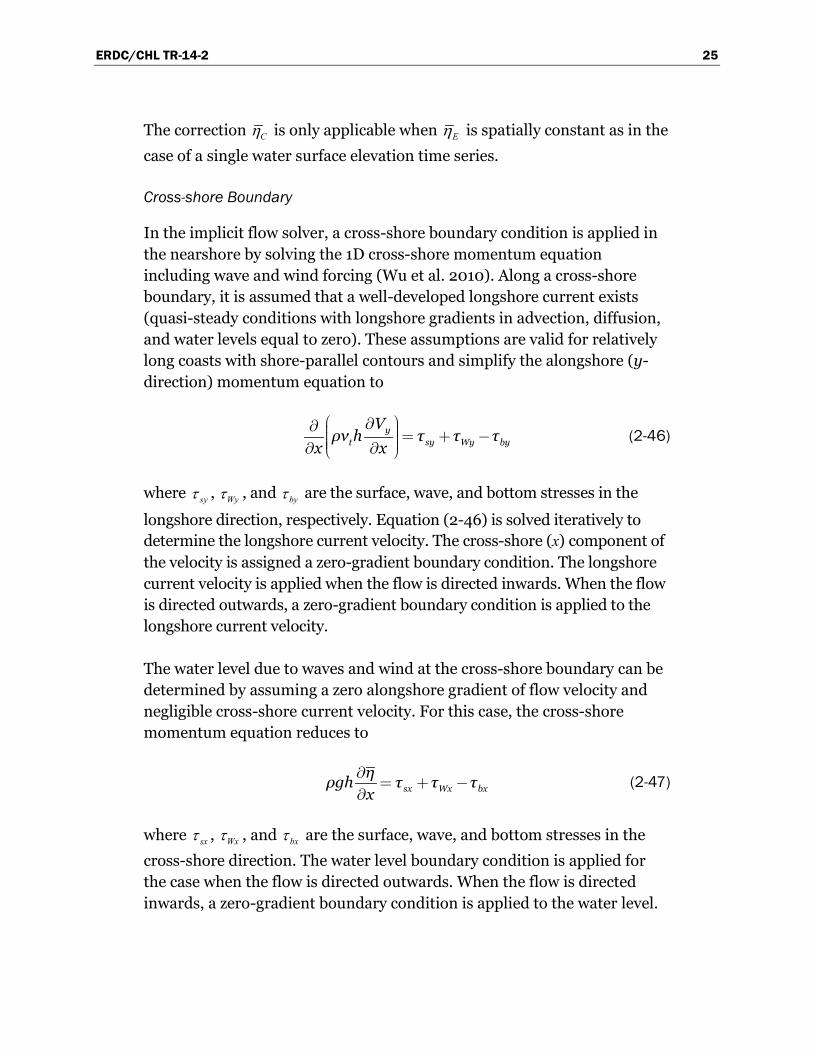
Cross-shore Boundary

In the implicit flow solver, a cross-shore boundary condition is applied in the nearshore by solving the 1D cross-shore momentum equation including wave and wind forcing (Wu et al. 2010). Along a cross-shore boundary, it is assumed that a well-developed longshore current exists (quasi-steady conditions with longshore gradients in advection, diffusion, and water levels equal to zero). These assumptions are valid for relatively long coasts with shore-parallel contours and simplify the alongshore (y-direction) momentum equation to

yt sy Wy by

Vρν h τ τ τ

x x

(2-46)

where syτ , Wyτ , and byτ are the surface, wave, and bottom stresses in the

longshore direction, respectively. Equation (2-46) is solved iteratively to determine the longshore current velocity. The cross-shore (x) component of the velocity is assigned a zero-gradient boundary condition. The longshore current velocity is applied when the flow is directed inwards. When the flow is directed outwards, a zero-gradient boundary condition is applied to the longshore current velocity.

The water level due to waves and wind at the cross-shore boundary can be determined by assuming a zero alongshore gradient of flow velocity and negligible cross-shore current velocity. For this case, the cross-shore momentum equation reduces to

sx Wx bxηρgh τ τ τx

(2-47)

where sxτ , Wxτ , and bxτ are the surface, wave, and bottom stresses in the

cross-shore direction. The water level boundary condition is applied for the case when the flow is directed outwards. When the flow is directed inwards, a zero-gradient boundary condition is applied to the water level.

ERDC/CHL TR-14-2 26

Salinity Transport

Overview

The characteristics of salinity are important in the coastal environment because salinity can impact marine plants and animals and influence the dynamic behavior of cohesive sediments. Because modifications of coastal inlets, such as channel deepening and widening and rehabilitation or extension of coastal structures, may alter the salinity distribution within estuaries or bays, it is often useful and convenient to simulate the salinity within the scope of an engineering project to determine if a more detailed water quality modeling study is necessary. It is important to emphasize that the CMS is not intended to be used as a water quality model. The CMS solves the depth-averaged (2DH) salinity transport equation and should be used only for cases where the water column is well mixed. If there is flow stratification, a 3D model should be utilized. It is also noted that the salinity is not used to update the water density which is assumed to be constant. Thus any horizontal water density gradients due to varying salinity on the hydrodynamics are assumed to be negligible.

Transport Equation

CMS calculates the salinity transport based on the following 2DH salinity conservation equation (Li et al. 2012):

( )( ) j salsal sal

sal salj j j

hV ChC Cν h S

t x x x

(2-48)

where:

salC = depth-averaged salinity [usually in ppt or psu]

h = water depth [m] jV = total flux velocity [m/s]

salν = horizontal mixing coefficient /sal t salν ν σ= [m2/s] tν = total eddy viscosity [m2/s] salσ = Schmidt number for salinity (approximately equal to 1.0) [-] salS = source/sink term [ppt m/s].

The above equation represents the horizontal fluxes of salt in water bodies and is balanced by exchanges of salt via diffusive fluxes. Major processes

ERDC/CHL TR-14-2 27

that influence the salinity are as follows: seawater exchange at ocean boundaries, freshwater inflows from rivers, precipitation and evaporation at the water surface, and groundwater fluxes (not included here).

Initial Condition

The initial condition for salinity transport may be specified as a constant, a spatially variable dataset usually calculated from a previous simulation or by solving a 2DH Laplace equation:

salC 2 0 (2-49)

where 2∇ is the Laplace operator. The equation is solved given any number of user-specified initial salinity values at locations within the model domain, using the initial salinity values at open boundaries and applying a zero-gradient boundary condition at all closed boundaries.

Boundary Conditions

At cell faces between wet and dry cells, a zero-flux boundary condition is applied. A salinity time series must be specified at all open boundaries and is applied when the flow is directed inward of the modeling domain. If the flow is directed outward of the modeling domain, then a zero-gradient boundary condition is applied.

Sediment Transport

Overview

For sand transport in coastal waters, the wash-load (i.e., sediment transport which does not appreciably contribute to the bed material) can be assumed to be negligible, and, therefore, the total-load transport is equal to the sum of the bed- and suspended-load transports. There are currently three sediment transport models available in CMS:

1. equilibrium total load (ET) 2. equilibrium bed load plus non-equilibrium suspended load (EBNS) 3. non-equilibrium total-load (NET).

The main differences among the three models are the assumption of local equilibrium transport for the bed and suspended loads. The ET model assumes that both the bed and suspended loads are in local equilibrium

ERDC/CHL TR-14-2 28

and solves a simple mass conservation equation known as the Exner equation. It is the least computationally intensive but can lead to model instabilities due to the assumption of local equilibrium transport. The EBNS model solves a transport equation for the depth-averaged suspended-load concentration, while the bed load is assumed to be in equilibrium and is included in a bed change equation. Using a non-equilibrium formulation for suspended load is more realistic and provides more accurate results. However, it still assumes that the bed load is in local equilibrium. A more realistic approach is to use non-equilibrium formulations for both the bed and suspended loads as in the NET model. The NET implemented in the CMS combines the bed- and suspended-load transport equations into a single total-load transport equation thus reducing the computational costs. The ET and EBNS models are only available using a single sediment size and with the explicit hydrodynamic temporal scheme. They are described in detail in Buttolph et al. (2006) and are not repeated here. The third model is available with both the explicit and implicit schemes. The support for multiple grain sizes is currently only in the NET model with the implicit time-stepping scheme. The multiple-sized non-equilibrium sediment transport model is introduced in this section.

Non-equilibrium Total-Load Transport Model

Total-load Transport Equation

The single-sized sediment transport model described in Sánchez and Wu (2011a) was extended to multiple-sized sediments within CMS by Sánchez and Wu (2011b). In this model, the sediment transport is separated into current- and wave-related transports. The transport due to currents includes the stirring effect of waves, and the wave-related transport includes the transport due to asymmetric oscillatory wave motion as well as steady contributions by Stokes drift, surface roller, and undertow. The current-related bed and suspended transports are combined into a single total-load transport equation, thus reducing the computational costs and simplifying the bed change computation. The 2DH transport equation for the current-related total load is

*

( ) ( )j tktk sk tks t sk tk tk

tk j j j

hU ChC r Cν h α ω C C

t β x x x

(2-50)

ERDC/CHL TR-14-2 29

for , ; , ,...,j k N 1 2 1 2 , where N is the number of sediment size classes and

tkC = actual depth-averaged total-load sediment concentration

[kg/m3] for size class k defined as / ( )tk tkC q Uh in which tkq is the total-load mass transport

*tkC = equilibrium depth-averaged total-load sediment concentration

[kg/m3] for size class k and described in the equilibrium concentration and transport rates section

tkβ = total-load correction factor described in the Total-Load

Correction Factor section [-] skr = fraction of suspended load in total load for size class k

described in fraction of suspended sediments section [-] sν = horizontal sediment mixing coefficient described in the

horizontal sediment mixing coefficient section [m2/s] tα = total-load adaptation coefficient described in the adaptation

coefficient section [-] skω = sediment fall velocity [m/s].

In the above equation, the first term represents the temporal variation of tkC ; the second term represents the horizontal advection; the third term

represents the horizontal diffusion and dispersion of suspended sediments; and the last term represents the erosion and deposition. The equation may be applied to single-sized sediment transport by using a single sediment size class (i.e., N = 1). The bed composition, however, does not vary when using a single sediment size class. The units of sediment concentration used here are kg/m3 rather than dimensionless volume concentrations in order to avoid numerical precision errors at low concentrations.

In the above equations, it is assumed that the wave flux velocity is not included in the momentum equations. If the wave flux velocity is included, then the total flux velocity (V ) should be used instead of the depth-averaged current velocity (U ). The reason for this is because without a wave-induced sediment transport to counter the offshore directed transport due to the undertow, the model would predict excessive movement of sediment offshore.

ERDC/CHL TR-14-2 30

Fraction of Suspended Sediment

In order to solve the system of equations for sediment transport implicitly, the fraction of suspended sediment must be determined explicitly. This is done by assuming

*

*

sk sksk

tk tk

q qr

q q (2-51)

where skq and tkq are the actual suspended- and total-load transport rates and *skq and *tkq are the equilibrium suspended- and total-load transport

rates.

Adaptation Coefficient

The total-load adaptation coefficient ( tα ) is an important parameter in the sediment transport model. There are many variations of this parameter in literature (Lin 1984; Gallappatti and Vreugdenhil 1985; and Armanini and di Silvio 1986). CMS uses a total-load adaptation coefficient ( tα ) that is related to the total-load adaptation length ( tL ) and time ( tT ) by

t tt s

UhL UTα ω

(2-52)

where:

sω = sediment fall velocity corresponding to the transport grain size

for single-sized sediment transport or the median grain size for multiple-sized sediment transport [m/s]

U = depth-averaged current velocity [m/s] h = water depth [m].

The adaptation length or time is a characteristic distance or time for sediment to adjust from non-equilibrium to equilibrium transport. Because the total load is a combination of the bed and suspended loads, the associated adaptation length may be calculated as (1 )t s s s bL r L r L= + − or

max( , )t s bL L L= , where sL and bL are the suspended- and bed-load

adaptation lengths. The symbol sL is defined as

ERDC/CHL TR-14-2 31

s ss

UhL UTαω

(2-53)

in which α and sT are the adaptation coefficient lengths for suspended load. The adaptation coefficient (α ) can be calculated either empirically or based on analytical solutions to the pure vertical convection-diffusion equation of suspended sediment. One example of an empirical formula is that proposed by Lin (1984):

*

. . ln sωα

κu

3 25 0 55 (2-54)

where *u is the bed shear stress, and κ is the von Karman constant.

Armanini and di Silvio (1986) proposed an analytical equation:

/

*

exp . sωδ δ δα h h h u

1 61 1 1 5 (2-55)

where δ is the thickness of the bottom layer defined by 033zδ = , and 0z is

the zero-velocity distance from the bed. Gallappatti (1983) proposed the following equation to determine the suspended-load adaptation time:

.* *

* *

. . . .exp

. ln . . .

r r

s

r r

u ω u ωhT

u u ω u

3 2 2047 21 57 20 12 326 832 0 2

0 1385 6 4061 0 5467 2 1963 (2-56)

where *u is the current related bottom shear velocity, * /ru u U= , and

* */sω ω u .

The bed-load adaptation length ( bL ) is generally related to the dimension of

bed forms such as sand dunes. Large bed forms are generally proportional to the water depth, and, therefore, the bed-load adaptation length can be estimated as b bL a h in which ba is an empirical coefficient on the order of

5-10. Although limited guidance exists on methods to estimate bL , the determination of bL is still empirical and in the developmental stage. For a

detailed discussion of the adaptation length, the reader is referred to Wu (2007). In general, it is recommended that the adaptation length be

ERDC/CHL TR-14-2 32

calibrated with field data in order to achieve the best and most reliable results.

Total-Load Correction Factor

The total-load correction factor ( tkβ ) accounts for the vertical distribution

of the suspended sediment concentration and velocity profiles as well as the fact that bed load travels at a slower velocity than the depth-averaged current velocity (Figure 2-3) (Wu 2007). By definition, tkβ is the ratio of

the depth-averaged total-load and flow velocities.

Figure 2-3. Schematic of sediment and current vertical profiles.

In a combined bed-load and suspended-load model, the correction factor is given by

( )tk

sk sk sk bk

βr β r U u

11

(2-57)

where bku is the bed-load velocity, and skβ is the suspended-load correction

factor and is defined as the ratio of the depth-averaged suspended sediment and flow velocities. Since most sediment is transported near the bed, both the total- and suspended-load correction factors ( tkβ and skβ ) are usually

less than 1 and typically in the range of 0.3 and 0.7, respectively. By assuming logarithmic current velocity and exponential suspended sediment concentration profiles, an explicit expression for the suspended-load correction factor ( skβ ) may be obtained as (Sánchez and Wu 2011b)

( )

E ( ) E ( ) ln( / )e ln( / )e

e ln( / ) e

k k

b

k k

b

η

Akz a k ksk η A A

kz a

uc dz A A Z Zβ

ZU c dz

1 1

1

1

1 1 1

φ φ

φ φ

φ φ (2-58)

ERDC/CHL TR-14-2 33

where:

/k sk kω h εφ [-] /A a h [-] /aZ z h [-]

kε = vertical mixing coefficient [m2/s]

a = reference height near the bed for the suspended load [m] az = apparent roughness length [m]

E ( )t

x

ex dtt

1 (exponential integral).

The equation can be further simplified by assuming that the reference height is proportional to the apparent roughness length (e.g., 30 aa z= ) so

that ,sk sk kβ β Z φ . Figure 2-4 shows a comparison of the suspended-load

correction factor based on the logarithmic velocity with exponential and Rouse suspended sediment concentration profiles. Both cases show similar behavior for the suspended-load correction factor ( skβ ). For fine sediments (small fall velocity), skβ is close to 1.0 and experiences smaller influences by the bottom roughness, while for course sediments, skβ can

be as low as 0.5 and is largely influenced by the bottom roughness. This is to be expected since course sediments are transported more closely to the bottom, compared to fine sediments.

Figure 2-4. Suspended load correction factors based on the logarithmic velocity profile and (a) exponential and (b) Rouse suspended sediment profile. The Rouse number is */ ( )sr uω κ= .

a.

b.

The bed-load velocity ( bku ) in Equation (2-57) is calculated using the van

Rijn (1984a) formula with re-calibrated coefficients from Wu et al. (2006):

ERDC/CHL TR-14-2 34

.

. ( )bbk k

crk

τu s gd

τ

0 5

1 64 1 1 (2-59)

where:

s = specific gravity [-] g = gravitational constant (~9.81 m/s2) kd = characteristic grain diameter for the kth size class [m]

/( / )b bτ n n τ 3 2 = grain-related bed shear stress [Pa] / /n d 1 6

50 20 = grain-related Manning’s roughness coefficient

[s/m1/3] crkτ = critical bed shear stress for the kth size class [Pa].

Bed Change Equation

The fractional bed change is calculated as

*b b

s m t sk tk tk s bkj jk

z zρ p α ω C C D q

t x x

1 (2-60)

where:

bz = bed elevation with respect to the vertical datum [m] mp′ = bed porosity [-] sρ = sediment (material) density (~2650 kg/m3 for quartz

sediment) sD = empirical bed-slope coefficient (constant) [-]

( )bk tk skq hUC r 1 is the bed-load mass transport rate magnitude

[kg/m/s].

The first term on the right-hand side of the above equation represents the bed change due to sediment exchange near the bed. The last term accounts for the effect of the bed slope on bed-load transport. The bed-slope coefficient ( sD ) is usually about 0.1 to 3.0. For a detailed derivation of the

above equation, the reader is referred to Sanchez and Wu (2011a). The total bed change is calculated as the sum of the bed changes for all size classes:

b b

k k

z zt t

(2-61)

ERDC/CHL TR-14-2 35

Bed Material Sorting and Layering

Bed sorting is the process in which the bed material changes size composition (fraction of each grain size class). The bed is discretized into multiple layers to consider the heterogeneity of bed material size composition along the bed depth. The fraction of each size class is then calculated and stored in each layer. The sorting of sediments is then calculated using the mixing or active layer concept (Hirano 1971; Karim and Kennedy 1982; Wu 1991). The mixing layer is the top layer of the bed which exchanges directly with the sediment moving in the water column. In other words, only the sediment in the mixing layer exchanges with the moving sediment in the water column; whereas, the sediment in the subsurface layers below the mixing layer does not directly exchange or contact with the moving sediment.

The temporal variation of the bed-material gradation in the first (mixing or active) layer is calculated as (Wu 2007)

*( )k b bk

k

δ p z zδp

t t t t

1 1 11 (2-62)

where:

1δ = thickness of the first layer [m] 1kp = fraction of the kth sediment size in the first layer [-]

* for / /

for / /k b

kk b

p z t δ tp

p z t δ t

1 11

2 1

0

0 [-]

2kp = fraction of the thk sediment size in the second layer [-].

The first term in Equation (2-62) corresponds to the erosion and deposition due to the thk sediment size while the second term corresponds to the sediment exchange between the first and second bed layers (Figure 2-5).

At the beginning of each time-step, the mixing or active layer thickness is calculated as

min maxmin max( , , . ),rδ δ d H δ1 502 0 5 (2-63)

ERDC/CHL TR-14-2 36

Figure 2-5. Multiple bed layer model of bed material sorting (after Wu 2007).

where rH is the ripple height, and minδ and maxδ are user-specified

minimum and maximum layer thicknesses, respectively.

The bed-material sorting in the second layer is calculated as

*( )k bk

δ p zδp

t t t

2 2 11 (2-64)

where 2δ is the thickness of the second layer. It is noted that there is no

material exchanged between the sediment layers below the second layer.

The sediment transport, bed change, and bed gradation equations are solved simultaneously (coupled) but are decoupled from the flow calculation at each time-step.

Sediment Fall Velocity

The sediment fall velocity may be user-specified or is calculated using the formula by Soulsby (1997):

/

*. . .sνω dd

1 22 310 36 1 049 10 36 (2-65)

where:

ν = kinematic viscosity [m2/s] d = grain size [m] *d = dimensionless grain size [-].

a. Erosion

Exchange between

1st and 2nd

layers

Δzb

t t+Δt

Δzb

t t+Δt

Mixing (1st)Layer

b. Deposition

ERDC/CHL TR-14-2 37

The dimensionless grain size is given by

/

*( )s gd d

ν

1 3

2

1 (2-1)

where:

s = sediment specific gravity or relative density [-] g = gravitational constant (9.81 m/s2).

Equilibrium Concentrations and Transport Rates

In order to close the system of equations describing the sediment transport, bed change, and bed sorting equations, the fractional equilibrium depth-averaged total-load concentration ( *tkC ) must be

estimated from an empirical formula. The depth-averaged equilibrium concentration is defined as

**

tktk

qC

Uh (2-67)

where *tkq is the total-load transport for the kth sediment size class

estimated from an empirical formula. For convenience, *tkC is written in

general form as

**tk k tkC p C 1 (2-68)

where 1kp is the fraction of the sediment size (k) in the first (top) bed layer, and *

tkC is the potential equilibrium total-load concentration. The potential

concentration ( *tkC ) can be interpreted as the equilibrium concentration

for uniform sediment of size kd . The above equation is essential for the

coupling of sediment transport, bed change, and bed sorting equations.

Lund-CIRP

Camenen and Larson (2005, 2007, 2008) developed general sediment transport formulas for bed and suspended loads under combined waves and currents. These are referred to as the Lund-CIRP transport formulas. The general transport formulas can be used for both symmetric and

ERDC/CHL TR-14-2 38

asymmetric waves, but for simplicity the waves are assumed to be symmetric. The current-related bed- and suspended-load transport with wave stirring is given by

*,

ΘΘ Θ exp .

Θ( )b cr

b s c cw mcw

qf ρ

s gd

350

12 4 51

(2-69)

* exp( )

s ss s R

s

q ω hεf ρ c Uω εs gd

350

11

(2-70)

where:

*bq = equilibrium bed-load transport rate [kg/m/s]

*sq = equilibrium suspended-load transport rate [kg/m/s]

cΘ = Shields parameters due to currents [-]

,cw mΘ = mean Shields parameters due to waves and currents [-] cwΘ = maximum Shields parameters due to waves and currents [-] crΘ = critical Shields parameter [-]

ε = vertical sediment diffusivity [m2/s] Rc = reference bed concentration [kg/m3] bf = bed-load scaling factor (default 1.0) [-] sf = suspended-load scaling factor (default 1.0) [-].

The critical Shields parameter is calculated using Equation (2-100). The mean and maximum Shields parameters are calculated as

, , ,Θ Θ Θ Θ Θ coscw m c w m c w m φ 2 2 2 (2-71)

Θ Θ Θ Θ Θ coscw c w c w φ 2 2 2 (2-72)

The mean wave Shields parameter is calculated as ,Θ Θ /w m w 2 assuming

a sinusoidal wave. The Shields parameters for currents and waves are given by

||Θ

( )c w

c ws

τg ρ ρ d

(2-73)

ERDC/CHL TR-14-2 39

in which the subscript c|w indicates either the current- (c) or wave-related (w) component. The current-related shear stress ( cτ ) is calculated with

Equation (2-11). The wave-related bed shear stress is calculated with Equation (2-12) and the wave friction factor ( wf ) of Swart (1974) given by

Equation (2-15).

The total bed roughness is assumed to be a linear summation of the grain-related roughness ( sgk ), form-drag (ripple) roughness ( srk ), and sediment-

related roughness ( ssk ):

, | , | , |s c w sg sr c w ss c wk k k k (2-74)

Here, the grain-related roughness is estimated as 502sgk d= . The ripple

roughness ( srk ) is calculated as (Soulsby 1997)

, |, |

, |

. r c wsr c w

r c w

Hk

L

2

7 5 (2-75)

where rH and rL are the ripple height and length, respectively.

The current- and wave-related sediment roughnesses are estimated as

, | |Θss c w c wk d 505 (2-76)

The above equation must be solved simultaneously with the expressions for the bottom shear stress because the roughness depends on the stress.

The reference concentration is given by

,

ΘΘ exp .

Θcr

R cR cw mcw

c A

4 5 (2-77)

where the coefficient cRA is determined by the following relationship:

*. exp .cRA d 0 0035 0 3 (2-78)

The vertical sediment diffusivity is calculated as

ERDC/CHL TR-14-2 40

/eD

ε hρ

1 3

(2-79)

where eD is the total effective dissipation given by

e b br c c w wD k D k D k D 3 3 3 (2-80)

in which bk , ck , and wk are coefficients; brD is the wave breaking dissipation (from the wave model); and cD and wD are the bottom friction

dissipation due to currents and waves, respectively. The dissipation from bottom friction due to current ( cD ) and the dissipation from bottom friction due to waves ( wD ) are expressed as

| | * |c w c w c wD τ u (2-81)

The coefficient bk =0.017 (Camenen and Larson 2008), and ck and wk are

a function of the Schmidt number:

| |c w c wκk σ6

(2-82)

where |c wσ is either the current- or wave-related Schmidt number

calculated from the following relationships (Camenen and Larson 2008):

| |

* | * ||

* || |

* |

sin for

( )sin for

s sc w c w

c w c wc w

c w sc w c w

s c w

ω ωπa bu u

σu ωπa bω u

2

2

12

1 1 12

(2-83)

with the coefficients .ca 0 4 , .cb 3 5 , .wa 0 15 , and .wb 1 5 .

For multiple-sized (non-uniform) sediments, the fractional equilibrium sediment transport rates are calculated as (Wu and Lin 2011)

*,

ΘΘ Θ exp .

Θ( )bk crk

b k k s c cw mcwk

qf ξ p ρ

s gd

1

1312 4 5

1 (2-84)

ERDC/CHL TR-14-2 41

* exp( )

sk k sks k k s Rk

sk kk

q ε ω hf ξ p ρ c U

ω εs gd

113

11

(2-85)

where:

k = subscript indicating the sediment size class kξ = hiding and exposure function [-]

skr = fraction of suspended load for each size class defined by Equation (2-51) [-]

1kp = fraction of the kth sediment size in the first layer [-].

The availability of sediment fractions is included through 1kp , while hiding and exposure of grain sizes are accounted for by directly multiplying the transport rates.

Van Rijn

The van Rijn (1984a,b) equations for bed-load and suspended-load transport are used with the recalibrated coefficients of van Rijn (2007a,b) as given by

. .

* .( )

e crb b s

U U dq f ρ Uh

hs gd

1 5 1 250

50

0 0151

(2-86)

.

.* *.

( )e cr

s s sU U

q f ρ Ud ds gd

2 4

0 650

50

0 0121

(2-87)

where:

crU = critical depth-averaged velocity for incipient motion [m/s] eU = effective depth averaged velocity [m/s].

The effective depth-averaged velocity is calculated as e wU U γu with γ = 0.4 for random waves and γ = 0.8 for regular waves. The bottom wave orbital velocity based on linear wave theory is uw. For random waves,

w wsu u= where wsu is based on the significant wave height and peak wave period (see Equation 2-24). The critical depth-averaged velocity is

ERDC/CHL TR-14-2 42

estimated as (1 )cr c crc c crwU U uβ β= + − where / ( )c wU U uβ = + is a blending factor. The critical depth-averaged current velocity ( crcU ) is given by Equation (2-102), and the critical bottom-wave-orbital velocity amplitude ( crwu ) is given by Equation (2-103).

According to van Rijn (2007a), the bed-load transport formula predicts transport rates by a factor of 2 for velocities higher than 0.6 m/s, but under predicts transport rates by a factor of 2 to 3 for velocities close to the initiation of motion.

The van Rijn formulas (1984a,b; 2007a,b) were originally proposed for well-sorted sediments. The sediment availability is included by multiplication of transport rates with the fraction of the sediment size class in the upper bed layer. The hiding and exposure are considered by a correction factor which multiples to the critical velocity. When applied to multiple-sized sediments, the fractional equilibrium transport rates are calculated as

. ./

* .( )e k crk k

bk b s kk

U ξ U dq f ρ p Uh

hs gd

1 5 1 21 2

1 0 0151

(2-88)

.

/.

* *.( )e k crk k

sk s s k kk

U ξ U dq f ρ p Uh d

hs gd

2 41 2

0 61 0 012

1 (2-89)

The availability of sediment fractions is included through 1kp , while hiding and exposure of grain sizes are accounted for by multiplying the critical velocity ( crkU ) by a correction function ( 1/2

kξ ).

Soulsby-van Rijn

Soulsby (1997) proposed the following equation for the total load sediment transport rate under action of combined current and waves:

. .

* .( )

e crcb b s

U U dq f ρ Uh

hs gd

2 4 1 250

50

0 0051

(2-90)

.

.* *.

( )e crc

s s sU U d

q f ρ Uh dhs gd

2 4

0 650

50

0 0121

(2-91)

ERDC/CHL TR-14-2 43

where:

.e rms

b

U U uc

2 20 018 = effective velocity [m/s]

rmsu = root-mean-square bottom wave orbital [m/s] crcU = critical depth-averaged velocity for initiation of motion for

currents based on Van Rijn (1984c) [m/s].

The bed friction coefficient ( bc ) is calculated using Equation (2-9) with the bed roughness length ( 0z ) set to 0.006 m following Soulsby (1997).

The Soulsby-van Rijn formula is modified for multiple-sized sediments similarly to the van Rijn formula in the previous section with the equation

. ./

* .)

e k crk kbk b s k

k

U ξ U dq f ρ p Uh

hs gd

2 4 1 21 2

1 0 0051

(2-92)

.

/.

* *.)

e k crk ksk s s k k

k

U ξ U dq f ρ p Uh d

hs gd

2 41 2

0 61 0 012

1 (2-93)

As in the case of the van Rijn transport formula, the availability of sediment fractions is included through 1kp , while hiding and exposure of grain sizes is accounted for by multiplying the critical velocity ( crkU ) by a correction function ( 1/2

kξ ). It is noted that the Soulsby-van Rijn (Soulsby

1997) formulas are very similar to the van Rijn (1984a,b; 2007a,b) except for the definition of the effective velocity and the recalibration of the bed-load formula coefficients in van Rijn (2007a). The proposed changes for multiple-sized sediments should be verified with measurements or numerical simulations for non-uniformly-sized sediment transport.

Watanabe

The equilibrium total-load sediment transport rate is determined by Watanabe (1987) as

max* ( ) b cr

t s s b s s Watτ τ

q f r f r ρ A Uρg

1 (2-94)

ERDC/CHL TR-14-2 44

where:

*tq = potential total-load transport rate [kg/m/s] sr = fraction of suspended load defined by Equation (2-51) [-] maxbτ = combined wave-current maximum shear stress [Pa] crτ = critical shear stress of incipient motion [Pa] WatA = empirical coefficient typically ranging from 0.1 to 2.0 [-].

The critical shear stress is determined from Equations (2-100) and (2-101). The maximum bed shear stress ( maxbτ ) is calculated as (Soulsby

1997)

max cos sinb b w wτ τ τ φ τ φ 2 2 (2-95)

where ϕ is the angle between the waves and current; bτ is the mean shear stress due to waves and currents; and wτ is the wave-related bed shear

stress which is calculated here using Equations (2-12) and (2-13).

The fraction of suspended sediment ( sr ) is estimated using the van Rijn

(2007a,b) transport equations described above. Besides being needed in the total-load transport equation (Equation 2-50), it also allows the application of the bed- and suspended-load scaling factors in a way similar to all other transport formula.

The Watanabe (1987) transport formula is modified for multiple-sized sediments as

max* ( ) b k crk

tk s sk b sk s k Watτ ξ τ

q f r f r ρ p A Uρg

11 (2-96)

where the subscript k indicates the sediment size class.

Hiding and Exposure

When the bed material is composed of multiple grain sizes, larger grains have a greater probability of being exposed to the flow while smaller parti-cles have a greater probability of being hidden from the flow. Figure 2-6 shows an example of a sediment grain ( jd ) being hidden by kd .

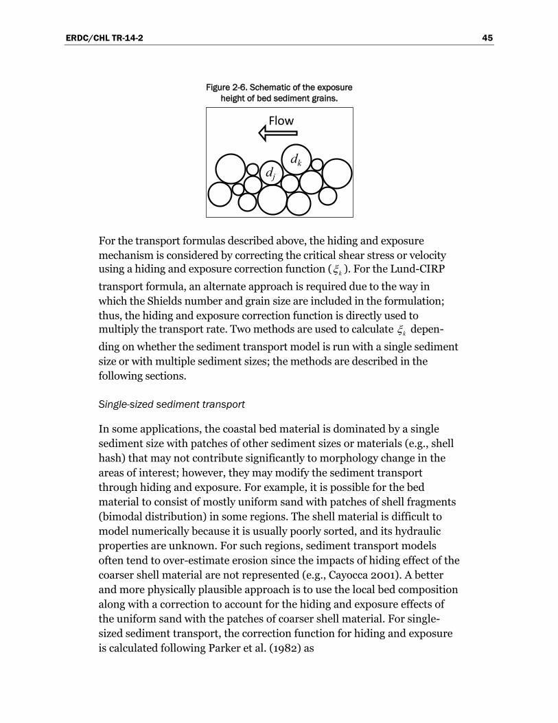
ERDC/CHL TR-14-2 45

Figure 2-6. Schematic of the exposure height of bed sediment grains.

For the transport formulas described above, the hiding and exposure mechanism is considered by correcting the critical shear stress or velocity using a hiding and exposure correction function ( kξ ). For the Lund-CIRP

transport formula, an alternate approach is required due to the way in which the Shields number and grain size are included in the formulation; thus, the hiding and exposure correction function is directly used to multiply the transport rate. Two methods are used to calculate kξ depen-

ding on whether the sediment transport model is run with a single sediment size or with multiple sediment sizes; the methods are described in the following sections.

Single-sized sediment transport

In some applications, the coastal bed material is dominated by a single sediment size with patches of other sediment sizes or materials (e.g., shell hash) that may not contribute significantly to morphology change in the areas of interest; however, they may modify the sediment transport through hiding and exposure. For example, it is possible for the bed material to consist of mostly uniform sand with patches of shell fragments (bimodal distribution) in some regions. The shell material is difficult to model numerically because it is usually poorly sorted, and its hydraulic properties are unknown. For such regions, sediment transport models often tend to over-estimate erosion since the impacts of hiding effect of the coarser shell material are not represented (e.g., Cayocca 2001). A better and more physically plausible approach is to use the local bed composition along with a correction to account for the hiding and exposure effects of the uniform sand with the patches of coarser shell material. For single-sized sediment transport, the correction function for hiding and exposure is calculated following Parker et al. (1982) as

Flow

dkdj

ERDC/CHL TR-14-2 46

m

kk

dξ

d

50

(2-97)

where m is an empirical coefficient between 0.5 to 1.0. The aforementioned sediment transport equations are implemented by using the transport grain size ( kd )rather than the bed material ( 50d ). A single and constant transport size ( kd ) is used, while the bed material ( 50d ) varies spatially. The spatial distribution of 50d can be obtained from field

measurement data and, for simplicity, is assumed constant during the model simulation time. This is a significant assumption and may not be reasonable for some applications. However, this method provides a simple conceptual mechanism for considering an important process in the proposed single-sized sediment transport model. The approach has been successfully applied to Shinnecock Inlet, NY, to simulate morphology change at a coastal inlet (Sánchez and Wu 2011a). A more accurate and complex approach is to simulate the transport and sorting of multiple-sized sediments.

Multiple-sized sediment transport

The hiding and exposure correction for each sediment size class is based on Wu et al. (2000):

m

ekk

hk

Pξ

P

(2-98)

where m is an empirical coefficient that varies for each transport formula, approximately equal to 0.6-1.0. The total hiding and exposure probabilities ( ekP and hkP , respectively) are calculated as

N

jhk j

j k j

dP p

d d

1

1

, N

kek j

j k j

dP p

d d

1

1

(2-99)

where N is the number of grain-size classes.

Incipient Motion

In the case of the Lund-CIRP (Camenen and Larson 2005, 2007, 2008) and Watanabe (1987) formulas, the incipient motion is based on the

ERDC/CHL TR-14-2 47

critical Shields parameter and estimated using the formula proposed by Soulsby (1997):

**

.Θ . exp .

.cr dd

0 3 0 055 1 0 02

1 1 2 (2-100)

in which the dimensionless grain size ( *d ) is defined in Equation (2-66).

The critical shear stress for incipient motion is given by

Θ( )

crcr

s

τg ρ ρ d

(2-101)

The critical depth-averaged velocity for currents alone ( crcU ) is calculated

using the formula proposed by van Rijn (1984c):

.

.

. log , for . . mm

. log , for . . mmcrc

hd dd

Uhd d

d

0 150 10 50

90

0 650 10 50

90

40 19 0 1 0 5

48 5 0 5 2 0

(2-102)

where 50d and 90d are the sediment grain size in meters of 50th and 90th

percentiles, respectively. The above criteria are used in the van Rijn (2007a,b) and Soulsby-van Rijn (Soulsby 1997) transport formulas.

The critical bottom orbital velocity magnitude for waves alone is calculated using the formulation of Komar and Miller (1975):

. . .

. . .

. , for . . mm

. , for . . mm

p

crw

p

s g d T dU

s g d T d

0 66 0 33 0 3350 50

0 57 0 43 0 1450 50

0 24 1 0 1 0 5

0 95 1 0 5 2 0 (2-103)

where pT is the peak wave period.

Ripple Dimensions

The bed forms calculated by CMS are the wave- and current-related ripples. The ripple height (used to calculate the mixing layer thickness) is estimated as the maximum of the current- and wave-related ripple heights

ERDC/CHL TR-14-2 48

, ,max( , )r r c r wH H H . (2-104)

The current-related ripple height and length are calculated as (Soulsby 1997)

, , /r c r cH L 7 (2-105)

,r cL d 501000 . (2-106)

The wave-related ripple height and length are calculated using the expressions proposed by van Rijn (1984b, 1989):

,

. for

. ( ) forfor

w w

r w w w w

w

A ψ

H ψ A ψψ

13 5

0 22 10

2 8 10 250 10 2500 250

(2-107)

.,

. for

. ( ) forfor

w w

r w w w w

w

A ψ

L ψ A ψψ

6 2 5

1 25 10

1 4 10 250 10 2500 250

(2-108)

where:

wA = semi-orbital excursion wu Tπ

2

[m/s]

wψ = wave mobility parameter = ( )

wus gd

2

501 [-]

50d = median grain size [m]

s = sediment specific gravity [-] g = gravitational constant (9.81 m/s2)

wu = bottom orbital velocity [m/s] (for random waves 2w rmsu u= ) T = wave period [s] (for random waves pT T= ).

The current- and wave-related ripple height and length are used in calculating the bed form roughness for use in the Lund-CIRP transport formula.

ERDC/CHL TR-14-2 49

Horizontal Sediment Mixing Coefficient

The horizontal sediment mixing coefficient ( sν ) represents the combined

effects of turbulent diffusion and dispersion due to non-uniform vertical profiles. In CMS, the horizontal sediment mixing coefficient is assumed to be proportional to the total eddy viscosity as

/s t sν ν σ (2-109)

where sσ is the Schmidt number, and tν is the total eddy viscosity. There

are many formulas to estimate the Schmidt number; however, for simplicity, it is assumed to be constant here. The default value for the Schmidt number is equal to 1.0 but may be modified by the user.

Boundary Conditions

At closed boundaries (interface between wet and dry cells), the sediment transport rate normal to the boundary is set to zero. The inflow boundary condition requires a given sediment concentration at the boundary. However, for most coastal applications, the actual sediment concentration is not available, and the model implements the equilibrium concentration. The equilibrium concentration is the concentration that is reached under steady and horizontally uniform conditions. If the flow is directed outward of the domain, a zero-gradient boundary condition is used for sediment concentration.

ERDC/CHL TR-14-2 50

3 Numerical Methods

Overview

CMS-Flow has both implicit and explicit solution schemes. The explicit solver is designed for dynamic problems with extensive wetting and drying that require small computational time-steps, while the implicit solver is intended for simulating tidal- and wave-induced circulation at tidal inlets, navigation channels, and adjacent beaches. A detailed description of the numerical formulation of the explicit solver of CMS-Flow can be found in Buttolph et al. (2006) and is not repeated here. The sections below specifically refer to the implicit solver of CMS-Flow.

The implicit solver uses the SIMPLEC (Semi-Implicit Method for Pressure Linked Equations Consistent) algorithm (van Doormal and Raithby 1984) on a non-staggered grid to handle the coupling of water level and velocity. Primary variables u-, v-velocity, and water level are stored on the same set of grid points, and fluxes at cell faces are determined using a Rhie and Chow (1983) type momentum interpolation method (Wu et al. 2011). The explicit solver uses a staggered grid with velocities at the cell faces and the water levels and water depths at the cell centers (Buttolph et al. 2006). CMS-Flow also calculates salinity, sediment transport, and morphology change. The governing equations for hydrodynamics and sediment and salinity transport have similar forms which can be written as a general transport (advection-diffusion) equation. In order to avoid redundant derivations of discretized equations, the discretization of the general transport equation is described in this chapter, and the same discretization may be applied to all of the transport equations. Then, the specific solution procedures for hydrodynamics, sediment transport, and bed change are introduced.

Computational Grid

The explicit time scheme in CMS-Flow supports uniform and non-uniformly spaced Cartesian grids while the implicit version of CMS-Flow supports generic Cartesian grids which can be uniform, non-uniform, or telescoping. The telescoping locally refines the mesh by splitting a cell into subcells. The only requirement imposed by the numerical methods is that the cells must have a rectangular shape. Additional requirements are

ERDC/CHL TR-14-2 51

imposed by the user interface which limits the variety of types of Cartesian grids to help simplify the grid generation and avoid grid quality issues. The following requirements are applied:

1. Cells can only be subdivided into four subcells. 2. Only two neighboring cells are allowed in the same direction (i.e., north,

south, east, and west). 3. Cells may have a maximum of six neighbors. 4. Refinement levels must be spaced by at least one cell apart (i.e., cells that

share the same corner must be one refinement level apart).

Examples of violations of the above four requirements are shown in sequential order in Figure 3-1 from a to d. Limiting the number of neighboring cells to six avoids excessive cell refinement and limits the band width of the coefficient matrix for the linearlized system of equations solved by the implicit solution scheme. The last two requirements avoid having excessive cell refinement which can cause numerical instabilities. The first requirement simplifies the grid generation process but may be relaxed in future versions. The last requirement is enforced for grid quality purposes and a more smoothly varying grid resolution.

Figure 3-1. Examples of invalid Cartesian computational grids.

a.

b.

c.

d.

ERDC/CHL TR-14-2 52

The CMS-Flow grids generated in the SMS interface can be classified as uniform, non-uniform Cartesian grids, regular telescoping, and stretched telescoping grids (Figure 3-2).

Figure 3-2. Types of Cartesian grids supported by the SMS interface and CMS-Flow.

One important aspect of incompressible flow models is the location of primary variables: velocity and pressure (water level). On a staggered grid, the pressure (water level) is located at the center of cells and the u- and v-velocities are located along the faces of cells (Harlow and Welsh 1965; Patankar 1980). On a non-staggered grid, all of the primary variables are located at the center of cells. This can lead to the spatial oscillations referred to as checkerboard oscillations and model instability if the linear interpola-tion between nodes is used to determine the fluxes at cell faces. A staggered grid can more easily eliminate these oscillations when compared to a non-staggered grid; however, a non-staggered grid involves a simpler source code and can minimize the number of coefficients that must be computed and stored during a simulation because many of the terms in the equations are equal. In particular, a staggered grid is more complicated when handling

Regular or Uniform

Regular Telescoping

Stretched Telescoping

Non-uniform

ERDC/CHL TR-14-2 53

the interface between coarse and fine cells where 5- or 6-face control volumes are used. Therefore, a non-staggered (collocated) grid approach is adopted for CMS-Flow with a Rhie and Chow (1983) momentum interpolation technique used to eliminate the checkerboard oscillations. Figure 3-3 shows the location of primary variables on the 5- and 7-point stencils (computational molecule).

Figure 3-3. Computational stencils and control volumes for two types of Cartesian grids: non-uniform Cartesian (left) and telescoping grid (right).

The data structure for a grid can be approached in three ways: 1) block-structured, 2) hierarchical tree, and 3) unstructured. The block-structured approach divides the domain into multiple blocks, and each block is treated as structured. The block structured approach requires a special treatment between blocks to ensure mass and momentum balance using this approach. The hierarchical tree approach is memory intensive and requires parent-child relationships and a tree traverse to determine mesh connectivity. For the unstructured approach, all cells are numbered in a 1D sequence, and tables are used to determine the connectivity of neighboring cells. Among these three approaches, the unstructured approach is the most simple and is therefore applied in CMS-Flow. Computational cells are numbered in an unstructured manner via a 1D index array. Inactive cells (permanently dry) are not included in the 1D index array to save memory and computational time. All active computational cells are numbered sequentially. It is noted that using an unstructured data approach does not limit the model from using matrix solvers designed for structured grids. For convenience with handling boundary conditions, each boundary cell has a neighboring ghost cell outside of the computational domain.

ERDC/CHL TR-14-2 54

General Transport Equation

The general transport equation is given by

Source Term

Temporal Term Advection Term Diffusion Term

( )Γj

j j j

hVh h St β x x x

φφ φ (3-1)

where:

φ = general scalar h = total water depth [m] β = correction factor [-] jV = total flux velocity [m/s] Γ = diffusion coefficient for φ [m2/s] S = source/sink term which includes all remaining terms.

Note that in the case of the continuity and momentum equations, φ is equal to 1 and iV , respectively. In the case of sediment and salinity transport, φ is equal to tkC and salC , respectively. The correction factor ( β ) is equal to the

total-load correction factor and equal to 1 for all other equations.

Spatial Discretization

A control-volume technique is used in which the governing equations are integrated over a control volume to obtain an algebraic equation that can be solved numerically. Integration of Equation (3-1) over a control volume (shaded areas in Figure 3-3) yields the following:

d Γ d djj jA A A

h A hV h A S At β x x

φ φφ (3-2)

ˆ ˆΔ Γ d ΔP PP i i i i P P

P L

hA h n V n L S A

t β

φ φ φ (3-3)

Δ Γ Δ ΔP PP f f f f f P Pf

fP

hA h V l S A

t β

φ φ φ (3-4)

ERDC/CHL TR-14-2 55

where:

ˆ ˆ ˆ( , )in n n 1 2 = outward unit vector normal to cell face f [-] ˆ( )f i i fV n V = outward cell face velocity [m/s]

Pφ = value of φ at the cell centroid Ph = total water depth at the cell centroid [m] fh = interpolated total water depth at cell face f [m]

f φ = outward normal gradient of φ at cell face f; f φ ˆi i fn φ

fΓ = interpolated diffusion coefficient for φ

PA∆ = area of cell P [m/s] fl∆ = length of cell face f [m]

PS = source/sink term.

In the above equations, the Gauss Divergence Theorem has been used to convert the area integral to a boundary integral. In addition, the area integrals have been evaluated assuming variables vary linearly within cells. The cell face velocity ( fV ) is calculated using a momentum interpolation

method similar to that of Rhie and Chow (1983) and is described in Hydrodynamics of the present Chapter.

Temporal Discretization

The general transport equation is rewritten as

G

ht β

φ (3-5)

where G includes all the remaining terms. For stability and efficiency, a fully implicit time-stepping scheme is used in the form

ˆ ˆ ˆ ˆ( . ) ( ) . GΔ

n n n n n nn

n n n

h h hθ θ θ

t β β β

1 1 1 11

1 1

1 1 0 5 1 0 5φ φ φ (3-6)

where θ is a weighting factor between 0 and 1. For θ = 0, the scheme reduces to the first-order backward Euler scheme, and with θ = 1, the scheme reduces to the second-order backward scheme (Ferziger and Peric 1997). The superscripts indicate the time-step levels, with n+1 being the

ERDC/CHL TR-14-2 56

next time-step, n being the current time-step, and n-1 being the previous time-step.

Cell-face Interpolation

The general formula for estimating the cell-face value ( fφ ) is given by

( ) ( )f N P N Pf f f r f r 1 1

φ φ φ φ φ (3-7)

where f⊥ is a linear interpolation factor, ∇

is the gradient operator in the direction parallel to face f, and r

is the distance from the cell center to the ghost point (O) parallel to the cell face ( f ) (Figure 3-4).

Figure 3-4. Schematic showing interface interpolation: (a) coarse to fine and (b) fine to coarse.

The subscripts and ⊥ indicate the components parallel and normal to the cell face. By definition, ˆ ˆn n 1 22 1 and ˆ ˆn n 1 21 2 . Note that

for neighboring cells without any refinement, r

is equal to zero, and the

above equation is consistent with non-refined cell faces. The linear interpolation factor is defined as

, , ,

, , , ,

ΔΔ Δ

f P P

N P P N

x x xf

x x x x

(3-8)

where , fx⊥ is the coordinate of f perpendicular to the face, and x⊥∆ is the

cell dimension perpendicular to the face f.

ERDC/CHL TR-14-2 57

Cell-face Gradient

A linearly exact second-order approximation for the normal gradient at cell face f is calculated using the auxiliary node concept of Ferziger and Peric (1997):

( ) N P N Pf

r r

δ δ

φ φφ φφ (3-9)

where the subscripts P and N refer to two neighboring cells,

, ,N Pδ x x is the distance between cells P and N, normal to the cell

face (Figure 3-4), and ∇

is the gradient operator in the direction parallel to

face f. Ham et al. (2002) compared the auxiliary node formulation to the fully-unstructured discretization proposed by Zwart et al. (1998) for the viscous terms and found that the auxiliary node formulation is significantly more stable.

Cell-centered Gradient

The cell-centered gradient operator is calculated using the Gauss’ Divergence Theorem as

ˆd Δi i f f

fA

A n l φ φ (3-10)

The equation above is second order and conservative for regular and non-uniform grids.

Reconstruction, Monotonicity, and Slope Limiters

Variables are linearly reconstructed within the cells as

P Pr

φ φ φ (3-11)

where Pφ is the cell-average value specified at the cell centroid, r is the

distance vector from the cell centroid to any location within the cell, and Pφ∇ is the cell-centered gradient. The reconstruction is second order and

conservative in the sense that ΔP P AA dA φ φ . The linear reconstruction is

used when interpolating cell-face values (Equation 3-7) and calculating

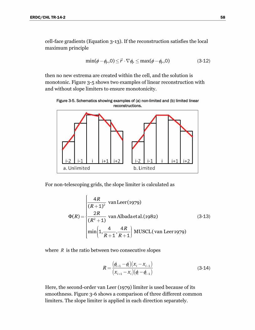
ERDC/CHL TR-14-2 58

cell-face gradients (Equation 3-13). If the reconstruction satisfies the local maximum principle

min( , ) max( , )P P Pr 0 0

φ φ φ φ φ (3-12)

then no new extrema are created within the cell, and the solution is monotonic. Figure 3-5 shows two examples of linear reconstruction with and without slope limiters to ensure monotonicity.

Figure 3-5. Schematics showing examples of (a) non-limited and (b) limited linear reconstructions.

For non-telescoping grids, the slope limiter is calculated as

vanLeer(1979)( )

Φ( ) vanAlbadaetal.(1982)( )

min , , MUSCL( van Leer1979)

RR

RRR

RR R

2

2

41

21

4 411 1

(3-13)

where R is the ratio between two consecutive slopes

i i i i

i i i i

x xR

x x

1 1

1 1

φ φφ φ

(3-14)

Here, the second-order van Leer (1979) limiter is used because of its smoothness. Figure 3-6 shows a comparison of three different common limiters. The slope limiter is applied in each direction separately.

ERDC/CHL TR-14-2 59

Figure 3-6. Comparison of three different slope limiters.

For unstructured grids the slope limiters described above are difficult to implement because of the difficulty in defining forward and backward differences. For telescoping grids the following Limited Central Difference (LCD) slope limiting procedure of Hubbard (1999) is applied:

max( , )for ( ) max( , )

( )min( , )

Φ for ( ) min( , )( )

otherwise

N PP N P

P

N Pf P N P

P

rr

rr

00

00

1

φ φφ φ φ

φφ φ

φ φ φφ (3-15)

where P f Pr x x

. In the procedure outlined by Hubbard (1999), a scalar

limiter is then calculated as ( )min fΦ = Φ . Here, a directional limiter is

applied as Φ min Φi ff f i , which is less dissipative. Finally, the cell-

centered gradient is limited as

*Φi P i i P φ φ (3-16)

where *i Pφ∇ is the unlimited gradient.

10-1

100

101

0

0.2

0.4

0.6

0.8

1

R

Slo

pe L

imite

r

van Albadavan LeerMUSCL

ERDC/CHL TR-14-2 60

Advection Schemes

Hybrid Scheme

The hybrid scheme is composed of a first-order upwind scheme and a second-order central difference scheme. The cell-face advective value is given by

/ for

for

D C f

f

C f

P

P

2 2

2

φ φφ

φ (3-17)

where the subscripts D and C indicate the downstream and upstream values, and /Γf f fP V δ is the Peclet number at the cell face in which

, ,N Pδ x x . In the hybrid scheme, when the Peclet number is larger

than 2, the first-order upwind value is used; otherwise, the second-order central difference value is used.

Exponential Scheme

The exponential scheme interpolates the face value using an exact solution to the 1D steady advection-diffusion equation:

exp( )

exp( )f P f

N P f

P fP

11

φ φφ φ (3-18)

The exponential scheme has automatic upwinding and is stable but is usually less than second order.

Hybrid Linear/Parabolic Scheme

The Hybrid Linear/Parabolic Approximation (HLPA) scheme of Zhu (1991) may be written as

ˆ ˆfor

otherwiseC D C C C

fC

0 1φ φ φ φ φφ

φ (3-19)

where the subscripts D , C , and U indicate the first downstream and first and second upstream cells, respectively. The normalized variable ( Cφ ) is

determined based on the formulation of Jasak et al. (1999)

ERDC/CHL TR-14-2 61

,

ˆ C U D CC

D U CCδ

1

2φ φ φ φ

φφ φ φ

(3-20)

where , , ,C D Cδ x x . The HLPA scheme is second order. Choi et al.

(1995) found that the HLPA scheme has similar accuracy to the third-order SMARTER (Sharp and Monotonic Algorithm for Realistic Transport Efficiently Revised) and LPPA (Linear and Piecewise-Parabolic Approximation) schemes but is simpler and more efficient (Shin and Choi 1992; Choi et al. 1995).

Source/Sink Term

The source/sink term is linearized as (Patankar 1980)

C PP P P PS S S φ (3-21)

The coefficient PPS is required to be non-positive for stability.

Assembly of Algebraic Equations

Assembly refers to the process of combining terms to create a linear system of algebraic equations. The algebraic equation for each cell is obtained by first combining or assembling all of the terms. Then, the continuity equation is multiplied by 1n

pφ+ and is subtracted from the

transport equation. The resulting discretized equation for cell P is

n nP P N N

N

a a b 1 1φ φ (3-22)

where the subscript N refers to the neighboring cell sharing cell faces; Pa and Na are linear coefficients for 1n

Pφ+ and 1n

Nφ+ . The last term ( b ) contains

all the remaining terms. Applying a similar equation for all of the internal cells of a grid results in a system of algebraic equations. This set of equations is referred to as the discretized governing equations.

Implicit Relaxation

The right-hand side of the algebraic system of equations ( b ) generally contains deferred corrections and source terms which must be computed iteratively. This iteration loop is referred to as the outer loop, and the loop

ERDC/CHL TR-14-2 62

within the linear iterative solver (see Section Iterative Solvers) is referred to as the inner loop. Under-relaxation is often applied to stabilize the convergence of the outer iteration loop. Under-relaxation may be applied as ( )m n mα α 1 1 1φ φφ φ φ in which φα is an under-relaxation parameter (0 < φα ≤ 1). The superscript m indicates the previous iteration,

and superscript m+1 indicates the new relaxed value. A better approach is used here to introduce the under-relaxation directly in the algebraic system of equations (Majumdar 1988; Ferziger and Peric 1997) as

n n mPP N N P P

N

αaa b a

α α

1 1 1 φ

φ φ

φ φ φ (3-23)

This is referred to implicit under-relaxation and has the effect of making the coefficient matrix more diagonally dominant, thus improving convergence.

Iterative Solvers

The selection of an iterative solver is one of the key issues impacting the overall performance of the model. CMS has six iterative solvers available, and they are described in more detail below: 1) GMRES, 2) BiCGStab, 3) SIP, 4) ICCG, 5) Gauss-Seidel, and 6) Gauss-Seidel with Successive-Over-Relaxation. The default iterative solver is a variation of the GMRES (Generalized Minimum RESidual) method (Saad 1993). The original GMRES method (Saad and Schultz 1986) utilizes the Arnoldi process to reduce the coefficient matrix to the Hessenburg form and minimizes the norm of the residual vector over a Krylov subspace at each iterative step. The variation of the GMRES method used here allows changes in preconditioning at every iteration step (Saad 1993). The Incomplete Lower Upper Factorization ILUT (Saad 1994) is used as the preconditioner to speed up convergence. The GMRES solver is applicable to symmetric and non-symmetric matrices and leads to the smallest residual for a fixed number of iterations. However, the memory requirements and computa-tional costs become increasingly expensive for larger systems.

The BiCGStab (BiConjugate Gradient Stabilized) iterative solver is also a Krylov subspace solver and is applicable to symmetric and non-symmetric matrices (Saad 1996). BiCGStab also uses ILUT as a preconditioner (Saad 1994). The BiCGStab method can be viewed as a combination of the standard Biconjugate Gradient solver where each iterative step is followed

ERDC/CHL TR-14-2 63

by a restarted GMRES iterative step. One advantage of the BiCGStab iterative solver is that the memory requirements are constant for each iteration, and there are less computational costs when compared to the GMRES method (for less than four iterations).

The SIP (Strongly Implicit Procedure) iterative solver uses an Incomplete Lower Upper decomposition, which approximates the exact Lower Upper decomposition (Stone 1968). The method is specifically designed for algebraic systems of equations derived from partial differential equations. The implementation here is for a 5-point stencil and, therefore, only applies to nontelescoping grids.

The ICCG (Incomplete Cholesky preconditioned Conjugate Gradient) iterative solver is applicable to symmetric matrices such as the pressure correction equation (Ferziger and Peric 2002). The implementation here is also for a 5-point stencil and, therefore, can only be applied to nontelescoping grids.

The simplest iterative solvers implemented here are the point-implicit Gauss-Seidel solvers with or without Successive-Over-Relaxation. The Succesive-Over-Relaxation may speed up convergence but can also lead to model divergence (Patankar 1980). Even though the Gauss-Seidel method requires more iterations for convergence, the overall efficiency may be higher than the GMRES and BiCGStab because each iteration is computa-tionally inexpensive, and the code is efficiently parallelized. However, based on experience and testing, the GMRES and BiCGStab methods are usually more robust and perform better for large time-steps.

Convergence and Time-Stepping

During the iterative solution process, error is calculated and used to determine if a solution has converged, diverged, or stalled at an error below a set tolerance threshold. An estimate of the error in solving the general algebraic equation is given by

n nP N N P P

NP

r a a ba

1 11 φ φ (3-24)

The l2-norm of the residual errors is given by

ERDC/CHL TR-14-2 64

Pcells P

r r 22

(3-25)

Since this value depends on the total number of cells, the final statistic (referred to as the residual) that is used for estimating the model convergence is obtained by dividing the l2-norm by the square root of the number of cells:

m

c

rR

N 2 (3-26)

where cN is the number of computational cells. Simply stated, mR is

referred to as the normalized residual error, and the superscript refers to the iteration number. Also, mR is calculated for each variable that is solved at each iteration step of the solution process. Each equation has default maximum tolerances for determining if the solution has converged, diverged, or stalled. The maximum number of iterations that is imposed is set equal to M. A minimum of five iterations is required for the hydrodynamic equations, and a minimum of M/2 iterations is required for the sediment transport equations. Table 3-1 lists the default criteria to determine whether the iterative solution procedure has converged, requires a reduced time-step, or has diverged.

Table 3-1. Default criteria to determine whether the iterative solution procedure has converged, diverged, or requires a reduced time-step.

Variable Converged Reduce Time-Step Diverged

Current velocity, m/s If Rm<1x10-7 If Rm>1.0x10-3 If Rm>1.0x10-2 or |Ui|>10.0

Pressure-correction, m2/s2

If Rm<1x10-8 If Rm>1.0x10-4 If Rm >1.0x10-3 or |p|>50.0

Total-load concentration, kg/m3

If Rm <1x10-8 None If Rm >1.0x10-3 or Ctk<0

Salinity, ppt If Rm <1x10-6 None If Csal <0

For the implicit model, the time-steps for the hydrodynamics, sediment and salinity transport are the same in order to avoid mass conservation problems and for simplicity. If any of the time-step reduction criteria are met, then the time-step is reduced by half and a minimum number of two time-steps are calculated at the newly reduced time-step. If the last time-

ERDC/CHL TR-14-2 65

step converged properly, then the time-step is increased. The maximum time-step allowed is equal to the user-specified initial time-step.

Ramp Function

For most coastal applications, the model is initialized from a cold start, which means that the water level and current velocities are initially set to zero. When the model is initialized with anything other than zeros, this is referred to as a hot start. The ramp period allows the model to slowly transition from the specified initial conditions without shocking the system. The ramp function is defined here as

cos min ,RampRamp

tf πt

1 1 12 2

(3-27)

where t is the simulation time, and Rampt is the ramp duration. The ramp

function provides a smooth function for transitioning from the specified initial conditions and is plotted in Figure 3-7.

Figure 3-7. Ramp function used in CMS.

The ramp function is applied to the model forcing conditions, including the wave forcing, surface wind, sediment concentration capacity, and significant wave height, by direct multiplication of these parameters by the ramp function at each time-step during the ramp period. Boundary conditions are also slowly transitioned from the initial condition by direct multiplication of the boundary conditions by the ramp function at each time-step during the ramp period. The ramp period is usually on the order of a few hours to a few days and should not be confused with the spin-up

0 0.2 0.4 0.6 0.8 1 1.20

0.2

0.4

0.6

0.8

1

t/tramp

Ram

p Fu

nctio

n

ERDC/CHL TR-14-2 66

period. The spin-up period is the time it takes for the effects of the initial condition to disappear and can be much longer than the ramp period.

Hydrodynamics

Coupling of Velocity and Water Level – SIMPLEC Algorithm

The governing equations are solved in a segregated manner in which each governing equation is solved separately in a sequential manner within an iteration loop in order to obtain a converged solution. Coupling between the velocity (momentum) and water level (continuity) is achieved with the SIMPLEC algorithm (van Doormal and Raithby 1984). The main difficulty in solving the momentum equations is that the water level is not known a priori and must be calculated as part of the solution. The solution algorithm procedure is described below. First, an initial pressure * *p gρ η= is

estimated based on the previous time-step value. Then, the momentum equations are solved for the corresponding velocity:

* ** * *

*( )( ) j ii i

t ij j j i

hV VhV V h pν h St x x x ρ x

(3-28)

where *iS includes all the remaining terms. The cell face velocities are

calculated with a Rhie and Chow (1983) type interpolation method:

* * *Δ Pf Vf

P ff

A hV H α pa ρ

(3-29)

where * * *Δ PV

P

A hH V α pa ρ , Vα is the implicit relaxation coefficient

(set to 0.8 by default), and ( ) f denotes linear interpolation (see Implicit

Relaxation of the present Chapter). This method avoids the checkerboard oscillations associated with the collocated grid. It is noted that this approach is slightly different from that originally proposed by Rhie and Chow (1983) and used by several authors such as Lai (2010). This current approach was found to be significantly more stable.

Next, the velocity (V ′) and pressure corrections ( p′ ) are defined such that both the momentum and continuity equations are satisfied:

ERDC/CHL TR-14-2 67

*ni i iV V V 1 , *np p p 1 (3-30 a,b)

In the SIMPLEC algorithm, the velocity correction is related to the pressure correction by

i iV G p (3-1)

where

Δ PV

P

VN

P

Ahαρ a

Gα aa

1

Using / ( / ) / ( )h t p t gρ∂ ∂ = ∂ ∂ and substituting 1 *ni i iV V V+ ′= + in the

continuity equation yields the semi-discrete water level correction equation

**( . )( ) ( ) .

Δ

n nj

j j j

hVθ p p θ p θp phG

ρg t x x x

11 0 5 1 0 5.(3-32)

Note that at convergence, p′→0, 1 *np p+ = , 1 *ni iV V+ = , and the above

equation reduces to the continuity equation. Once the pressure correction equation is solved, the cell-centered water levels and current velocities are corrected. The cell face velocities are also corrected as *n

f f fV V V 1 , in

which the velocity correction is given by f f fV G p .

Summary of the SIMPLEC Algorithm:

1. Guess the water level and pressure field ( *p ). 2. Solve the momentum equations (Equation 3-28) to obtain *

iV .

3. Use the Rhie and Chow (1983) type momentum to determine the velocities and fluxes at cell faces (Equation 3-29).

4. Solve the pressure equation (Equation 3-34) to obtain p′ . 5. Use the correction equations to adjust the velocities and water levels. 6. Treat the corrected water level and pressure field as a new guess and

repeat this procedure from Step 2 until convergence is achieved.

ERDC/CHL TR-14-2 68

Wetting and Drying

During numerical simulations of the surface water flows with sloped beaches, sand bars, and islands, the land-water interface changes with time. This means that it is possible for nodes at the land-water interface to be wet or dry throughout a given simulation. In CMS, a threshold water depth is used to judge drying and wetting. If the depth at the cell center is larger than the threshold value (i.e., a small value such as 0.02 m for field cases), then the node is considered to be wet. Similarly, if the depth at the cell center is smaller than the threshold value, then the node is considered to be dry. For the implicit solver, all of the wet and dry cells are included in the matrix solver. Dry cells are assigned with a zero velocity.

Salinity Transport

Transport Equation

The salinity transport equation is discretized using the methods described in the previous section entitled General Transport Equation and are not repeated here.

Laplace Equation

The option is provided to estimate the initial salinity based on the solution of a 2DH Laplace equation with given boundary conditions and scattered salinity values. The Laplace equation is discretized similarly to the transport equation as

Δsal fff

C l 0 (3-33)

where:

( )sal fC⊥∇ = outward normal gradient of φ at cell face ( f )

fl∆ = length of cell face ( f ) [m].

Sediment Transport and Morphology Change

The so-called semi-coupled sediment transport model proposed by Wu (2004) is adopted here, in which the sediment calculations are decoupled from the hydrodynamic calculations, but the sediment transport, bed

ERDC/CHL TR-14-2 69

change, and bed material sorting equations are simultaneously solved in a coupled form at each time-step.

Transport Equations

The sediment transport equations are discretized using the methods described in the previous section entitled General Transport Equation and are not repeated here.

Bed Change Equations

The fractional bed change equation is discretized as

*

ΔΔ

( )morph n n n

bk t sk tk tk bks m

f tz α ω C C S

ρ p

1 1 1

1 (3-34)

where:

morphf = morphologic acceleration factor

( ) ΔΔ

n b sbk s bk bk f b ff

fj j

z DS D q q z l

x x A

1

sD = bed slope coefficient [-]

( )bk fq = magnitude of the fraction bed load at the cell face f calculated

from previous iteration [kg/m/s] b f

z = bed slope calculated at the cell face.

The purpose of the morphologic acceleration factor ( morphf ) is to speed up

the bed change so that the simulation time ( simt ) represents approximately the change that would occur in morph morph simt f t . This factor should be

used with caution and only for idealized cases or time periods which are periodic (mainly tidal). If time-varying winds or waves are important processes for driving sediment transport, then it is recommended to use reduced or representative wind and wave conditions. Since the CMS runs relatively fast, it is generally recommended not to use the morphologic acceleration factor when validating the sediment transport model using hindcast measurements. The morphologic acceleration factor is useful, however, when simulating idealized cases or analyzing project alternatives.

ERDC/CHL TR-14-2 70

Bed Material Sorting

The bed material sorting equation (Equation 2-53) is discretized as

*Δ Δn n n

n bk k kk n

z δ p z pp

δ

1 1 1 2

1 11

(3-35)

where Δ Δ n nbz z δ δ 1

2 1 1 is the change in the top elevation of the second bed layer, and *n n

k kp p 1 for 2 0z∆ ≥ and *n nk kp p 2 for 2 0z∆ < . The

mixing layer or active layer thickness calculation is slightly modified to avoid excessively small layers as

,min ,maxmin max( , ,Δ/ ),δ δ d δ 1 1 50 12 2 (3-36)

where ∆ is the bed form height, and 1,minδ and 1,maxδ are the user-

specified minimum and maximum mixing layer thicknesses, respectively.

The thickness of the second layer is calculated as Δn nδ δ z 12 2 2 . The bed

material gradation in the second layer is calculated from the following discretized form of Equation 2-54:

*Δn n n

n k kk n

δ p z pp

δ

1 2 2 2

2 12

(3-37)

In order to avoid sediment layers from becoming extremely thin or thick, a layer merging and splitting algorithm is implemented between layers 2 and 3. Here, the subscript 2 corresponds to the second layer. To illustrate the bed layering process, Figure 3-8 shows an example of the temporal evolution of seven bed layers during erosional and depositional regimes.

It is noted that in order to maintain a constant number of bed layers, the bottom two layers are merged if the second layer is split or a new layer is created at the bottom using the bed composition and thickness of the bottom layer.

Avalanching

When the slope of a non-cohesive bed ( bφ ) is larger than the angle of repose ( Rφ ), the bed material will slide (avalanche) to form a new slope

ERDC/CHL TR-14-2 71

Figure 3-8. Schematic showing an example bed layer evolution. Colors indicate layer number and not bed composition.

approximately equal to the angle of repose. The process of avalanching is simulated by enforcing b Rφ φ≤ while maintaining mass continuity

between adjacent cells. The following equation for bed change due to avalanching is obtained by combining the equation for angle of repose and the continuity equation between two adjacent cells:

,Δ

Δ tan sgn tan HΔ Δ

a N Nb p a b b R b R

N P N

A δz α

A A

φ φ φ φ φ (3-38)

where Nδ is the cell center distance between cells P and N , A∆ is the cell area, aα is an under-relaxation factor (approximately 0.25-0.5), and H( )X

is the Heaviside step-function representing the activation of avalanching and equal to 1 for X ≥0 and 0 for X <0. The sign function ( sgn X ) is equal to 1 for X ≥0 and -1 for X <0 and accounts for the fact that the bed slope may have a negative or positive sign. Equation (3-38) is applied by sweeping through all computational cells to calculate a

bz∆ and then modifying the bathymetry as Δm m a

b b bz z z 1 . Because avalanching between two cells may

induce additional avalanching at neighboring cells, the above sweeping process is repeated until avalanching no longer occurs. The under-relaxation factor ( aα ) is used to stabilize the avalanching process and to

avoid overshooting since the equation is derived considering only two adjacent cells but is summed over all (avalanching) neighboring cells. Equation (3-38) may be applied to any grid geometry type (i.e., triangles, rectangles, etc.) and for situations in which neighboring cells are joined at corners without sharing a cell face.

0 5 10 15 20-3.2

-3

-2.8

-2.6

-2.4

-2.2

-2

-1.8

Time step

Ele

vatio

n, m

ERDC/CHL TR-14-2 72

Hard bottom

The sediment transport and bed change equations assume a loose bottom in which the bed material is available for entrainment. However, hard bottoms may be encountered in practical engineering applications where bed materials are non-erodible, such as bare rocks, carbonate reefs, and concrete coastal structures. Hard bottom cells in CMS are handled by modifying the equilibrium concentration as * *min( , )t t tC C C′ = in both the

sediment transport and bed change equations. The bed slope term in the bed change equation is also modified so that only deposition (no erosion) may occur at hard-bottom cells.

Coupling of Sediment Transport, Bed Change, and Sorting Equations

For a semi-coupled sediment transport model, the sediment calculations are decoupled from the hydrodynamics, but the sediment transport, bed change, and bed material sorting equations are coupled at the time-step level and thus solved simultaneously. A modified form of the iteration procedure of Wu (2004) is implemented in CMS. The equations are obtained by substituting *

*n n nt k k tkC p C 1 1 1

1 into the bed change and sorting

equations and then substituting the sorting equation into the bed change equation.

Summary of Sediment Transport Semi-Coupling Procedure:

1. Calculate bed roughnesses and bed shear stresses. 2. Calculate the mixing layer thickness 1

1nδ + .

3. Calculate the potential sediment concentration capacity * 1ntkC + .

4. Guess the new bed composition as 11 1n nk kp p+ = .

5. Calculate the fractional concentration capacity 1 1 * 1* 1n n nt k k tkC p C+ + += .

6. Solve transport equations for each sediment size class for 1ntkC + .

7. Calculate the total and fractional bed changes. 8. Determine the bed sorting in the mixing layer; Repeat Step 5 and iterate

until convergence. 9. Update the bed elevation as 1n n

b b bz z z+ = + ∆ .

10. Calculate the bed gradation in the bed layers below the mixing layer. 11. Calculate avalanching. 12. Correct the sediment concentration due to flow depth change.

ERDC/CHL TR-14-2 73

When using the explicit time-stepping scheme, the sediment transport and morphology change are solved at a time-step which may be equal to or multiples of the hydrodynamic time-step for efficiency. However, when using the implicit time-stepping scheme, the time-step is relatively big and on the order of 10 min. Because the time-step is so big, it is not necessary to use different time-steps for hydrodynamics and sediment transport. In addition, using the same time-step for hydrodynamics and sediment transport provides a better mass balance. For these reasons, the sediment transport time-step is always set to the hydrodynamic time-step in the implicit time-stepping scheme.

Coupling Procedure of CMS-Flow and CMS-Wave

CMS-Flow and CMS-Wave can be run separately or coupled together using a process called steering (Figure 3-9). The variables passed from CMS-Wave to CMS-Flow are the significant wave height, peak wave period, wave direction, wave breaking dissipation, and radiation stress gradients. CMS-Wave uses the updated bathymetry (if sediment transport is turned on), water levels, and current velocities from CMS-Flow.

Figure 3-9. Coupling process between CMS-Flow and CMS-Wave.

The time interval at which the CMS-Wave model is run is called the steering interval. Currently, the steering interval is constant, and, therefore, the input spectra must be at constant intervals without any gaps. A schematic showing the steering process is shown in Figure 3-10 in which the simulations time is plotted as a function of the computational time.

Wave ModelSpectral Wave Transformation

Flow ModelHydrodynamics,

Sediment Transport and Morphology Change

Significant Wave Height Wave Mean Direction

Wave Peak PeriodRadiation Stress Gradients

Wave Dissipation

Effective Current VelocitiesWater Surface Elevation

Bed Elevation

ERDC/CHL TR-14-2 74

Figure 3-10. Schematic of steering process.

For CMS versions prior to version 4.0, the steering process is controlled in the SMS interface with communication files because the CMS-Wave and CMS-Flow models are separate executables. For CMS v4.0 and above, both CMS-Flow and CMS-Wave are contained within a single executable (known as the inline executable), and the steering process is controlled by an interval steering module. Two main advantages of the inline executable and inline steering module are as follows: 1) the model runs faster because there is no need to use communication files or reinitialize the models (memory allocation, variable initialization, etc.); and 2) the inline executable makes the improvement and maintenance of the steering module easier for the developers. The inline steering process is summarized as follows:

1. CMS-Wave is run for the first two time-steps, and the wave information is passed to CMS-Flow (Figure 3-10). If specified, the surface roller model is run on the wave grid, and the roller contributions to the radiation stresses are added to the wave radiation stresses.

2. The wave height, period, dissipation, radiation stress gradients, and wave unit vectors are interpolated spatially from the CMS-Wave grid to the CMS-Flow grid.

3. CMS-Flow is run until the next steering interval and wave variables are linearly interpolated throughout time during the specified steering interval. At each flow time-step, variables such as wave length and bottom orbital velocities are updated using the current water depths and current velocities.

CMS-FlowCMS-Wave

Steering Interval

Computational Time

Sim

ulat

ion

Tim

e

ERDC/CHL TR-14-2 75

4. Water levels, current velocities, and bed elevations are estimated for the next wave time-step and are interpolated from the CMS-Flow grid to the CMS-Wave grid.

5. CMS-Wave is then run again for the following time-step. 6. Step 2-5 are repeated until the end of the simulation.

Spatial Interpolation and Extrapolation

CMS allows the user to use the same or different grids for CMS-Flow and CMS-Wave. If the same grid is used, then no spatial interpolation is carried out. If different grids are used, then spatial interpolation is necessary in order to transfer information from one model grid to another model grid. The interpolation of wave variables from the CMS-Wave grid to the CMS-Flow grid is done using a combination of bilinear and linear triangular interpolation. Bilinear interpolation is applied at non-jointed cells (i.e., cells with four neighbors) and triangular interpolation at jointed cells (cells with more than four neighbors). If the extents of the CMS-Wave and CMS-Flow grids are different (e.g., if the CMS-Flow grid is smaller), then the extrapolation of variables is necessary in order to avoid boundary problems with the models. The spatial extrapolations for different variables are given by

m m

P Nwave flowη η (3-39)

, ,

m m

i P ext i Nwave flowU f U (3-40)

, , ,Δm m m

b P b P ext b Nwave wave flowz z f z

1 (3-41)

, ,

n n

s P ext s Nflow waveH f H (3-42)

, ,

n n

p P p Nflow waveT T (3-43)

n n

P Nflow wavew w

(3-44)

where η is the mean water surface elevation, iU is depth-averaged current velocities, bz is the bed elevation, sH is the significant wave height, pT is

ERDC/CHL TR-14-2 76

peak wave period, and w is the wave unit vector. The superscripts m and n indicate the CMS-Wave and CMS-Flow time-steps, respectively. The subscripts wave and flow indicate variables on CMS-Wave and CMS-Flow grids respectively. The subscripts P and N indicate variables at the extrapolated and nearest neighbor cells. The extrapolation function ( extf )

is given by

cos min ,Next

ext

rf π

r

1 1 12 2

(3-45)

Here, Nr is the distance from cell P to N, and extr is the extrapolation

distance. The extrapolation distance is assigned to each computational grid and can be either automatically calculated by CMS or specified by the user. The mean water surface elevation, peak wave period, and wave unit vectors are extrapolated using a nearest neighbor. This approach is more physically accurate than extrapolating only to a certain distance. For example, water levels are controlled mainly by tides along the coast, and the spatial variation is usually much smaller than the tidal range. Extrapolating bed elevations from a boundary can lead to sharp changes in bathymetry in the wave model and instability problems in both the wave and flow models. A better approach is to extrapolate the bed change. It is noted that this is only for extrapolation. For internal cells the actual bed elevations are interpolated from the flow grid to the wave grid. Finally, careful attention is needed in determining the nearest neighbor so that variables are not extrapolated over inactive portions of the grid (e.g., interpolating values in a bay using values from the open ocean).

Temporal Interpolation and Prediction

Because CMS-Wave requires the water surface elevation at times that are ahead of the hydrodynamic model, the water surface elevation and currents must be predicted for the CMS-Wave time-step. If the steering is relatively small (<30 min), then the values from the last time-step may be used without significant error as

m n

i iflow flowU U (3-46)

m n

flow flowη η (3-47)

ERDC/CHL TR-14-2 77

m n

b bflow flowz z (3-48)

where superscripts m and n indicate the CMS-Wave and CMS-Flow time-steps, respectively. The subscript flow indicates the variables on the CMS-Flow grid. For many coastal engineering applications, it is desirable and common to use relatively large steering intervals of 2 to 3 hours. For large steering intervals, the change in water depth has the largest influence on the nearshore wave heights. Therefore, when using large steering intervals, it is desirable to make better predictions of water levels without using the previous time-step water levels. In cases where the relative surface gradients at any time are much smaller than the mean tidal elevation, a better approximation of water level may be obtained by decomposing the water level into

m m mm vflow flow flow

η η η (3-49)

where mη is the mean water level, and vη is a variation around the mean

due to due to tidal, wave, and wind generated surface gradients. The symbol mη can be approximated from water level boundary conditions and is generally much larger. The water level variation ( vη ) may be neglected

or approximated using the last flow time-step as

m n n nv v mflow flow flow flow

η η η η (3-50)

For most coastal inlet applications, the above equation is a better representation of the water surface elevation and is used as the default in CMS. After spatially interpolating the wave variables (significant wave height, wave vector, peak wave period, wave breaking dissipation, and wave radiation stresses) onto the CMS-Flow grid, the wave variables are linearly interpolated in time. The wavelength, bottom orbital velocities, and mean wave-current bottom friction are then updated for current-wave interactions at each flow model time-step.

ERDC/CHL TR-14-2 78

4 Summary

The CMS is an integrated wave, current, sediment transport, and morphology change model available in the Surface-water Modeling System (SMS). The CMS was developed under the Coastal Inlets Research Program (CIRP), an Operations and Maintenance Navigation research program at the Coastal and Hydraulics Laboratory, Engineer Research and Development Center, US Army Corps of Engineers. The CMS consists of two main components: a spectral wave transformation model named CMS-Wave (Lin et al. 2008; 2011a,b) and a hydrodynamic, salinity, sediment, and morphology change model named CMS-Flow (Wu et al. 2010; Sánchez et al. 2011a,b).

Both CMS-Wave and CMS-Flow support regular and non-uniform Cartesian grids while the CMS-Flow supports regular, non-uniform, telescoping, and stretched telescoping Cartesian grids. The CMS-Wave and CMS-Flow models are tightly coupled within a single inline code. The CMS-Wave and CMS-Flow grids may be the same or have different spatial extents and resolutions.

CMS-Flow uses the Finite Volume Method and has both fully explicit and fully implicit time-stepping schemes. Detailed descriptions of the CMS-Flow mathematical formulations and explicit time-marching schemes are provided in Militello et al. (2004) and Buttolph et al. (2006) and are not repeated here. Several verification and validation tests were presented for hydrodynamics, sediment transport, and morphology change in Sánchez et al. (2011a,b). The present report provides an updated description of the mathematical formulations and implicit time marching schemes which have not been covered in previous CMS-Flow reports.

The hydrodynamic model solves the depth-integrated and wave-averaged hydrodynamic equations and includes physical processes such as advec-tion, turbulent mixing, combined wave-current bottom friction; wave mass flux; wind, atmospheric pressure, wave, river, and tidal forcing; Coriolis force; and the influence of coastal structures (Buttolph et al. 2006; Wu et al. 2010). The fully implicit hydrodynamic model uses the SIMPLEC (van Doormaal and Raithby 1984) algorithm on a collocated grid. The inter-cell velocities are calculated using a Rhie and Chow (1983) type momentum interpolation method.

ERDC/CHL TR-14-2 79

The implicit hydrodynamic model is integrated with a total-load nonequilibrium and multiple-sized sediment transport model and includes processes such as hiding and exposure, bed sorting and gradation, bed slope effects, nonerodible surfaces, and avalanching. The sediment transport model solves a depth-integrated and wave-averaged total-load sediment transport, bed sorting and change equations simultaneously using an iterative method. The salinity and sediment transport equations are solved on the same Cartesian grid as the hydrodynamics, and in the case of the implicit time-stepping scheme, use the same time-step as the hydrodynamics.

The latest guidance, documentation, and downloads for the Coastal Modeling System are available at http://cirp.usace.army.mil/ and from the CIRP wiki: http://cirp.usace.army.mil/wiki/Main_Page.

ERDC/CHL TR-14-2 80

References Andrews, D. G., and M. E. McIntyre. 1978. An exact theory of nonlinear waves on a

Lagrangian mean flow. Journal of Fluid Mechanics (89):609–646.

Armanini, A., and G. di Silvio. 1986. Discussion on the paper “A depth-averaged model for suspended sediment transport”, by G. Galappattti and C. B. Vreugdenhil. Journal of Hydraulic Research 24 (5):437–441.

Batten, B. K., and N. C. Kraus. 2006. Evaluation of downdrift shore erosion, Mattituck Inlet, New York: Section 111 Study. ERDC/CHL-TR-06-1. Vicksburg, MS: US Army Engineer Research and Development Center.

Beck, T. M., and N. C. Kraus. 2010. Shark River Inlet, New Jersey, entrance shoaling: Report 2, analysis with coastal modeling system. ERDC/CHL-TR-10-4. Vicksburg, MS: US Army Engineer Research and Development Center.

Beck, T. M., and K. Legault. 2012. St. Augustine Inlet, Florida: Application of the coastal modeling system. ERDC/CHL-TR-12-14. Vicksburg, MS: US Army Engineer Research and Development Center.

Buttolph, A. M., C. W. Reed, N. C. Kraus, N. Ono, M. Larson, B. Camenen, H. Hanson, T. Wamsley, and A. K. Zundel. 2006. Two-dimensional depth-averaged circulation model CMS-M2D: Version 3.0, Report 2: Sediment transport and morphology change. ERDC/CHL TR-06-9. Vicksburg, MS: US Army Engineer Research and Development Center.

Bye, J. A. T. 1985. Large-scale momentum exchange in the coupled atmosphere–ocean, coupled ocean–atmosphere models, 51–61. Amsterdam: Elsevier Science Publishers.

Byrnes, M. R., S. F. Griffee, and M. S. Osler. 2010. Channel dredging and geomorphic response at and adjacent to Mobile Pass, Alabama. ERDC/CHL-TR-10-8. Vicksburg, MS: US Army Engineer Research and Development Center.

Camenen, B., and M. Larson. 2005. A general formula for non-cohesive bed-load sediment transport. Estuarine, Coastal and Shelf Science (63)2:49–260.

Camenen, B., and M. Larson. 2007. A unified sediment transport formulation for coastal inlet application. ERDC/CHL CR-07-1. Vicksburg, MS: US Army Engineer Research and Development Center.

Camenen, B., and M. Larson. 2008. A general formula for noncohesive suspended sediment transport. Journal of Coastal Research 24 (3):615–627.

Cayocca, F. 2001. Long-term morphological modeling of a tidal inlet: the Arcachon Basin, France. Coastal Engineering (42):115–142.

Choi, S. K., H .Y. Nam, and M. Cho. 1995. A comparison of higher-order bounded convection schemes. Computational Methods in Applied Mechanics and Engineering (121):281-301.

ERDC/CHL TR-14-2 81

Coastal Engineering Manual (CEM). 2002. Engineer Manual 1110-2-1100. Washington, DC: US Army Corps of Engineers.

Dabees, M., and B. D. Moore. 2011. Inlet evolution modeling of multiple inlet systems in Southwest and Central Florida. Journal of Coastal Research, Special Issue (59):130–137.

Davies, A. G., R. L. Soulsby, and H. L. King. 1988. A numerical model of the combined wave and current bottom boundary layer. Journal of Geophysical Research 93(C1):491–508.

Dawe, J. T., and L. Thompson. 2006. Effect of ocean surface currents on wind stress, heat flux, and wind power input to the ocean. Geophysical Research Letters (3):3, L09604.

Dean, R. G., and R. A. Dalrymple. 1984. Water wave mechanics for engineers and scientists. Englewood Cliffs, NJ: Prentice-Hall.

Feddersen, F., R. T. Guza, S. Elgar, and T. H. C.Herbers. 2000. Velocity moments in alongshore bottom stress parameterizations. Journal of Geophysical Research 105(C4):8673–8686.

Ferziger, J. H., and M. Peric. 1997. Computational methods for fluid dynamics. Berlin/New York: Springer-Verlag.

Fredsoe, J. 1984. Turbulent boundary layer in wave-current motion. Journal of Hydraulic Engineering, ASCE (110):1103–1120.

Gallappatti, R., 1983. A depth-integrated model for suspended transport. Comunications on hydraulics, Vol. 83-7. Delft: Delft University of Technology.

Gallappatti, G., and C. B. Vreugdenhil. 1985. A depth-integrated model for suspended sediment transport. Journal of Hydraulic Research 23(4):359–377.

Graf, W. H., and M. Altinakar. 1998. Fluvial hydraulics. Hoboken, NJ: Wiley & Sons, Ltd.

Grant, W. D., and O. S. Madsen. 1979. Combined wave and current interaction with a rough bottom. Journal of Geophysical Research 86(C4):1797–1808.

Harlow, F. H., and J. E. Welch. 1965. Numerical calculation of time-dependent viscous incompressible flow of fluid with free surface. Physics of Fluids (8): 2182.

Hasselmann, K., T. P. Barnett, E. Bouws, H. Carlson, D. E. Cartwright, K. Enke, J. A. Ewing, H. Gienapp, D. E. Hasselmann, P. Kruseman, A. Meerbrug, P. Muller, D. J. Olbers, K. Richter, W. Sell, and H. Walden. 1973. Measurements of windwave growth and swell decay during the Joint North Sea Wave Project (JONSWAP). Deutsche Hydrographische Zeitschrift A80(12):95.

Hirano, M. 1971. River bed degradation with armouring. Transactions of the Japan Society of Civil Engineering 3(2):194–195.

Hsu, S. A. 1988. Coastal meteorology. San Diego, CA: Academic Press.

ERDC/CHL TR-14-2 82

Hubbard, M. E. 1999. Multidimensional slope limiters for MUSCL-type finite volume schemes on unstructured grids. Journal of Computational Physics (155):54–74.

Huynh-Thanh, S., and A. Temperville 1991. A numerical model of the rough turbulent boundary layer in combined wave and current interaction. In Sand transport in rivers, estuaries and the sea, ed. R. L. Soulsby and R. Bettess, 93–100. Rotterdam: Balkema.

Jasak, H., H. G., Weller, and A. D. Gosman. 1999. High resolution NVD differencing scheme for arbitrarily unstructured meshes. International Journal of Numerical Methods for Fluids (31):431–449.

Jonsson, I. G. 1966. Wave boundary layers and friction factors. In Proceedings of the 10th Coastal Engineering Conference, ASCE, 127–148.

Komar, P. D., and M. C. Miller. 1975. On the comparison between the threshold of sediment motion under waves and unidirectional currents with a discussion of the practical evaluation of the threshold. Journal of Sedimentary Petrology (45):362–367.

Lai, Y. G. 2010. Two-dimensional depth-averaged flow modeling with an un-structured hybrid mesh. Journal of Hydraulic Engineering (136):12–23.

Li, H., M. E. Brown, T. D. Smith, and J. H. Podoski. 2009. Evaluation of proposed channel on circulation and morphology change at Kawaihae Harbor and Pelekane Bay, Island of Hawaii, HI. ERDC/CHL TR-09-19. Vicksburg, MS: US Army Engineer Research and Development Center.

Li, H., L. Lin, M. E. Brown. 2011. Applying particle tracking model in the Coastal Modeling System. ERDC/CHL CHETN-IV-78. Vicksburg, MS: US Army Engineer Research and Development Center.

Li, H., C. W. Reed, and M. E. Brown. 2012. Salinity calculations in the Coastal Modeling System. ERDC/CHL CHETN-IV-80. Vicksburg, MS: US Army Engineer Research and Development Center.

Lin, B. N. 1984. Current study of unsteady transport of sediment in China. In Proceedings, Japan-China Bilateral Seminar on River Hydraulics and Engineering Experience, July, 337–342. Tokyo-Kyoto-Saporo, Japan.

Lin, L., Z. Demirbilek, H. Mase, J. Zheng, and F. Yamada. 2008. CMS-Wave: A nearshore spectral wave processes model for coastal inlets and navigation projects. ERDC/CHL TR-08-13. Vicksburg, MS: US Army Engineer Research and Development Center.

Lin, L., Z. Demirbilek, and H. Mase. 2011a. Recent capabilities of CMS-Wave: A coastal wave model for inlets and navigation projects. Journal of Coastal Research, Special Issue (59):7–14.

Lin, L., Z. Demirbilek, R. Thomas, and J. Rosati III. 2011b. Verification and validation of the coastal modeling system, report 2: CMS-WAVE. ERDC/CHL-TR-11-10. Vicksburg, MS: US Army Engineer Research and Development Center.

ERDC/CHL TR-14-2 83

Lin, L., J. Rosati III, and Z. Demirbilek. 2012. CMS-Wave model: Part 5: Full-plane wave transformation and grid nesting. ERDC/CHL CHETN-IV-81. Vicksburg, MS: US Army Engineer Research and Development Center.

Lin, L., H. Li, Brown, M. E. Wu, F., and L. Andes. 2013. Pilot study evaluating nearshore sediment placement sites, Noyo Harbor, CA. ERDC/CHL-TR-13-2. Vicksburg, MS: US Army Engineer Research and Development Center.

Longuet-Higgins, M. S., and R. W. Stewart. 1961. The changes in amplitude of short gravity waves on steady non-uniform currents. Journal of Fluid Mechanics 10(4):529–549.

MacDonald, N. J., M. H. Davies, A. K. Zundel, J. D. Howlett, T. C. Lackey, Z. Demirbilek, and J. Z. Gailani. 2006. PTM: Particle Tracking Model; Report 1: Model theory, implementation, and example applications. ERDC/CHL-TR-06-20. Vicksburg, MS: US Army Engineer Research and Development Center.

Madsen, O. S. 1994. Spectral wave–current bottom boundary layer flows. In Proceedings of the 24th Conference on Coastal Engineering, ASCE, 384–398. Kobe, Japan.

Majumdar, S. 1988. Role of underrelaxation in employing momentum interpolation practice for calculation of flow with non-staggered grids. Numerical Heat Transfer (13):125–132.

Mase, H., K. Oki, T. S. Hedges, and H. J. Li. 2005. Extended energy-balance-equation wave model for multidirectional random wave transformation. Ocean Engineering 32(8–9):961–985.

Mei, C. 1989. The applied dynamics of ocean surface waves. New York: John Wiley.

Militello, A., C. W. Reed, A. K. Zundel, and N. C. Kraus. 2004. Two-dimensional depth-averaged circulation model M2D: Version 2.0, Report 1, Technical documentation and user's guide. ERDC/CHL TR-04-02. Vicksburg, MS: US Army Engineer Research and Development Center.

Myrhaug, D., L. E. Holmedal, R. R. Simons, and R .D. MacIver. 2001. Bottom friction in random waves plus current flow. Coastal Engineering (43):75–92.

Nielsen, P. 1992. Coastal bottom boundary layers and sediment transport. Singapore: World Scientific.

Pacanowski, R. C. 1987. Effect of equatorial currents on surface wind stress. Journal of Physical Oceanography (17):833–838.

Parker, G., P. C., Kilingeman, and D. G. McLean. 1982. Bed load and size distribution in paved gravel-bed streams. Journal of the Hydraulics Division, ASCE 108(4):544–571.

Patankar, S. V. 1980. Numerical heat transfer and fluid flow. New York: Hemisphere,

Phillips, O. M. 1977. The dynamics of the upper ocean. (2nd Edition). Cambridge, England: Cambridge University Press.

ERDC/CHL TR-14-2 84

Powell, M. D., P. J., Vickery, and T. A. Reinhold. 2003. Reduced drag coefficient for high wind speeds in tropical cyclones. Nature (422):279–283.

Reed, C. W., and L. Lin. 2011. Analysis of Packery Channel public access boat ramp shoreline failure. Journal of Coastal Research, Special Issue (59):150–155.

Reed, C. W., M. E., Brown, A. Sánchez, W. Wu, and A. M. Buttolph. 2011. The Coastal Modeling System Flow Model (CMS-Flow): Past and Present. Journal of Coastal Research, Special Issue (59):1–6.

Rhie, T. M., and A. Chow. 1983. Numerical study of the turbulent flow past an isolated airfoil with trailing-edge separation. AIAA Journal (21):1525–1532.

Rosati, J. R., A. E., Frey, M. E., Brown, and L. Lin. 2011. Analysis of dredged material placement alternatives for bottleneck removal, Matagorda Ship Channel, Texas. ERDC/CHL-TR-11-2. Vicksburg, MS: US Army Engineer Research and Development Center.

Saad, Y., and M. H. Schultz. 1986. GMRES: A generalized minimal residual algorithm for solving nonsymmetric linear systems. SIAM Journal of Scientific and Statistical Computing (7):856–869.

Saad, Y. 1993. A flexible inner-outer preconditioned GMRES algorithm. SIAM Journal Scientific Computing (14):461–469.

Saad, Y. 1994. ILUT: a dual threshold incomplete ILU factorization. Numerical Linear Algebra with Applications (1):387–402.

Saad, Y. 1996. Iterative methods for sparse linear systems. Boston, MA: PWS Publishing Company.

Sánchez, A., and W. Wu. 2011a. A non-equilibrium sediment transport model for coastal inlets and navigation channels. Journal of Coastal Research, Special Issue (59):39–48.

Sánchez, A., and W. Wu. 2011b. Non-uniform sediment transport modeling at Grays Harbor, WA. In Proceedings, Coastal Sediments 2011, Vol. 3, 1783–1796. Miami, FL.

Sánchez, A., W. Wu, J. D. Rosati, Z. Demirbilek, L. Li, J. Rosati, R. Thomas, C. Reed, I. Watts, and M. Brown. 2011a. Validation of the coastal modeling system: Report III, Hydrodynamics. ERDC/CHL-TR-11-10 Vicksburg, MS: US Army Engineer Research and Development Center.

Sánchez, A., W. Wu, J. D. Rosati, Z. Demirbilek, L. Li, J. Rosati, R. Thomas, C. Reed, I. Watts, and M. Brown. 2011b. Validation of the coastal modeling system: Report IV, sediment transport and morphology change. ERDC/CHL-TR-11-10. Vicksburg, MS: US Army Engineer Research and Development Center.

Shin, J. K., and Y. D. Choi. 1992. Study on the improvement of the convective differencing scheme for the high-accuracy and stable resolution of the numerical solution [in Korean]. Transactions KSME 16(6):1179–1194.

ERDC/CHL TR-14-2 85

Shore Protection Manual (SPM). 1984. Shore protection manual. 4th ed., 2 Vol. US Army Engineer Waterways Experiment Station: US Government Printing Office.

Smagorinsky, J. 1963. General circulation experiments with the primitive equations. Monthly Weather Review 93(3):99–164.

Soulsby, R. L. 1987. Calculating bottom orbital velocity beneath waves. Coastal Engineering (11):371–380.

Soulsby, R. L. 1995. Bed shear-stresses due to combined waves and currents. In Advances in Coastal Morphodynamics, ed. M. J. F Stive, H. J. de Vriend, J. Fredsoe, L. Hamm, R. L. Soulsby, C. Teisson, and J. C. Winterwerp. Netherlands: Delft Hydraulics, 4-20 through 4-23.

Soulsby, R. L. 1997. Dynamics of marine sands. London, England: Thomas Telford Publications.

Soulsby, R. L., and R. J. S. W Whitehouse. 1997. Threshold of sediment motion in coastal environments. In Proceedings, Pacific Coasts and Ports '97 Conference, 1, 149–154. New Zealand: Christchurch, University of Canterbury.

Stone, H. L. 1968. Iterative solution of implicit approximations of multidimensional partial differential equations. SIAM Journal of Numerical Analysis 5(3):530–538.

Svendsen, I. A. 2006. Introduction to nearshore hydrodynamics. Singapore: World Scientific.

Swart, D. H. 1974. Offshore sediment transport and equilibrium. Beach profiles. Delft, The Netherlands: Delft Hydraulics Laboratory Publications.

van Albada, G. D., B. van Leer, and W. W. Roberts. 1982. A comparative study of computational methods in cosmic gas dynamics. Astronomy and Astrophysics (108):76–84.

van Doormaal, J. P. and Raithby, G. D. 1984. Enhancements of the SIMPLE method for predicting incompressible fluid flows. Numerical Heat Transfer (7): 147–163.

van Leer, B. 1979. Toward the ultimate conservative difference scheme. V. A second order sequel to Godunov method. Journal of Compuational Physics (32):101–136.

van Rijn, L. C. 1984a. Sediment transport, Part I: Bed-load transport. Journal of Hydraulic Engineering, ASCE 110(10):1431–1456.

van Rijn, L. C. 1984b. Sediment transport, Part II: Suspended-load transport. Journal of Hydraulic Engineering, ASCE 110(11):1613–1641.

van Rijn, L. C. 1984c. Sediment transport, Part III: Bed forms and alluvial roughness. Journal of Hydraulic Engineering, ASCE 110(12):1733–1754.

van Rijn, L. C. 1989. Handbook: Sediment transport by currents and waves. Delft, The Netherlands: Delft Hydraulics.

ERDC/CHL TR-14-2 86

van Rijn, L. C. 1998. Principles of coastal morphology. Amsterdam, The Netherlands: Aqua Publications.

van Rijn, L. C. 2007a. Unified view of sediment transport by currents and waves. Part I: Initiation of motion, bed roughness, and bed-load transport. Journal of Hydraulic Engineering 133(6):649–667.

van Rijn, L. C. 2007b. Unified view of sediment transport by currents and waves. Part II: Suspended Transport. Journal of Hydraulic Engineering 133(6):668–689.

Walstra, D. J. R., J. A. Roelvink, and J. Groeneweg. 2000. Calculation of wave-driven currents in a 3D mean flow model. In Proceedings, 27th International Conference on Coastal Engineering, 1050-1063. Sydney, Australia.

Wang, P., T. M. Beck, and T. M. Roberts. 2011. Modeling regional-scale sediment transport and medium-term morphology change at a dual inlet system examined with the Coastal Modeling System (CMS): A case study at Johns Pass and Blind Pass, West-central Florida. Journal of Coastal Research, Special Issue (59):49–60.

Watanabe, A. 1987. 3-dimensional numerical model of beach evolution. In Proceedings, Coastal Sediments ’87, 802–817. New Orleans, LA.

Wiberg, P. L., and C. R. Sherwood. 2008. Calculating wave-generated bottom orbital velocities from surface-wave parameters. Computers and Geosciences 34(10):1243–1262.

Wright, D. G., and K. R. Thompson. 1983. Time-averaged forms of the nonlinear stress law. Journal of Physical Oceanography (13):341–346.

Wu, W. 1991. The study and application of 1-D, horizontal 2-D and their nesting mathematical models for sediment transport. PhD diss. Wuhan, China: Wuhan University of Hydraulic and Electrical Engineering.

Wu, W., S. S. Y. Wang, and Y. Jia. 2000. Non-uniform sediment transport in alluvial rivers. Journal of Hydraulic Research, IAHR 38(6):427–434.

Wu, W. 2004. Depth-averaged 2-D numerical modeling of unsteady flow and non-uniform sediment transport in open channels. Journal of Hydraulic Engineering, ASCE 135(10):1013–1024.

Wu, W., M. Altinakar, and S. S. Y. Wang. 2006. Depth-averaged analysis of hysteresis between flow and sediment transport under unsteady conditions. International Journal of Sediment Research 21(2):101–112.

Wu, W. 2007. Computational river dynamics. United Kingdom: Taylor & Francis.

Wu, W., A. Sánchez, and M. Zhang. 2010. An implicit 2-D depth-averaged finite-volume model of flow and sediment transport in coastal waters. In Proceedings of the International Conference on Coastal Engineering, No. 32. Paper Number: Sediment 23. Shanghai, China.

ERDC/CHL TR-14-2 87

Wu, W., and Q. Lin. 2011. Extension of the Lund-CIRP formula for multiple-sized sediment transport under currents and waves. Oxford, MS: The University of Mississippi, National Center for Computational Hydroscience and Engineering.

Wu, W., A. Sánchez, and M. Zhang. 2011. An implicit 2-D shallow water flow model on an unstructured quadtree rectangular grid. Journal of Coastal Research, Special Issue (59):15–26.

Zarillo, G. A., and F. G. A. Brehin. 2007. Hydrodynamic and morphologic modeling at Sebastian Inlet, FL. In Proceedings of Coastal Sediments ’07, 1297–1311. New Orleans, LA: ASCE Press.

Zhu, J. 1991. A low-diffusive and oscillation-free convection scheme. Communications in Applied Numerical Methods (7):225–232.

Zwart, P. J., G. D., Raithby, and M. J. Raw. 1998. An integrated space-time finite volume method for moving boundary problems. Numerical Heat Transfer (B34):257.

Zundel, A. K. 2006. Surface-water modeling system reference manual – version 9.0. Provo, UT: Brigham Young University Environmental Modeling Research Laboratory.

REPORT DOCUMENTATION PAGE Form Approved

OMB No. 0704-0188 Public reporting burden for this collection of information is estimated to average 1 hour per response, including the time for reviewing instructions, searching existing data sources, gathering and maintaining the data needed, and completing and reviewing this collection of information. Send comments regarding this burden estimate or any other aspect of this collection of information, including suggestions for reducing this burden to Department of Defense, Washington Headquarters Services, Directorate for Information Operations and Reports (0704-0188), 1215 Jefferson Davis Highway, Suite 1204, Arlington, VA 22202-4302. Respondents should be aware that notwithstanding any other provision of law, no person shall be subject to any penalty for failing to comply with a collection of information if it does not display a currently valid OMB control number. PLEASE DO NOT RETURN YOUR FORM TO THE ABOVE ADDRESS. 1. REPORT DATE (DD-MM-YYYY)

March 2014 2. REPORT TYPE

TR 3. DATES COVERED (From - To)

4. TITLE AND SUBTITLE

Coastal Modeling System: Mathematical Formulations and Numerical Methods

5a. CONTRACT NUMBER

5b. GRANT NUMBER

5c. PROGRAM ELEMENT NUMBER

6. AUTHOR(S)

Alejandro Sánchez, Weiming Wu, Honghai Li, Mitch Brown, Chris Reed, Julie Rosati, Zeki Demirbilek, and Lihwa Lin

5d. PROJECT NUMBER

5e. TASK NUMBER

5f. WORK UNIT NUMBER

7. PERFORMING ORGANIZATION NAME(S) AND ADDRESS(ES) 8. PERFORMING ORGANIZATION REPORT NUMBER

Coastal and Hydraulics Laboratory, U.S. Army Engineer Research and Development Center 3909 Halls Ferry Road, Vicksburg, MS 39180-6199; National Center for Computational Hydroscience and Engineering, The University of Mississippi 327 Brevard Hall, University Road, Oxford, MX 38677; Reed & Reed Consulting 1400 Village Square Blvd Ste 3-146 Tallahassee, FL32312 3909

ERDC/CHL TR-14-2

9. SPONSORING / MONITORING AGENCY NAME(S) AND ADDRESS(ES) 10. SPONSOR/MONITOR’S ACRONYM(S) Headquarters, U.S. Army Corps of Engineers Washington, DC, 20314-1000

11. SPONSOR/MONITOR’S REPORT NUMBER(S)

12. DISTRIBUTION / AVAILABILITY STATEMENT Approved for public release; distribution is unlimited.

13. SUPPLEMENTARY NOTES

14. ABSTRACT

The Coastal Modeling System (CMS) is an integrated numerical modeling system for simulating nearshore waves, currents, water levels, salinity and sediment transport, and morphology change. The CMS was designed and developed for coastal inlets and navigation applications, including channel performance and sediment exchange between inlets and adjacent beaches. The present report provides an updated description of the mathematical formulations and numerical methods of hydrodynamic, salinity and sediment transport, and morphology change model CMS-Flow. The CMS-Flow uses the Finite Volume Method on Cartesian grids and has both fully explicit and fully implicit time stepping schemes. A detailed description of the explicit time stepping scheme was provided in Militello et al. (2004) and Buttolph et al. (2006). The present report focuses on the recent changes in the mathematical formulations, and the implicit time stepping schemes. The CMS-Wave and CMS-Flow models are tightly coupled within a single “inline” code. The CMS-Wave and CMS-Flow grids may be the same or have different spatial extents and resolutions. The hydrodynamic model includes physical processes such as advection, turbulent mixing, combined wave-current bottom friction; wave mass flux; wind, atmospheric pressure, wave, river, and tidal forcing; Coriolis force; and the influence of coastal structures. The implicit hydrodynamic model is coupled to a nonequilibrium transport model of multiple-sized total-load sediments. The model includes physical processes such as hiding and exposure, bed sorting and gradation, bed slope effects, nonerodible surfaces, and avalanching. 15. SUBJECT TERMS Coastal Sediment Transport

Morphology Change Hydrodynamics Waves

Numerical Methods Finite Volume Finite Difference

16. SECURITY CLASSIFICATION OF: 17. LIMITATION OF ABSTRACT

18. NUMBER OF PAGES

19a. NAME OF RESPONSIBLE PERSON Alejandro Sanchez

a. REPORT

UNCLASSIFIED

b. ABSTRACT

UNCLASSIFIED

c. THIS PAGE

UNCLASSIFIED 102 19b. TELEPHONE NUMBER (include area code)

Standard Form 298 (Rev. 8-98) Prescribed by ANSI Std. 239.18