coarse-to-fine mcmc in a seismic monitoring...
TRANSCRIPT
Coarse-to-fine MCMC in a seismic monitoring system
Xiaofei Zhou
Electrical Engineering and Computer SciencesUniversity of California at Berkeley
Technical Report No. UCB/EECS-2015-252
http://www.eecs.berkeley.edu/Pubs/TechRpts/2015/EECS-2015-252.html
December 18, 2015

Copyright © 2015, by the author(s).All rights reserved.
Permission to make digital or hard copies of all or part of this work forpersonal or classroom use is granted without fee provided that copies arenot made or distributed for profit or commercial advantage and that copiesbear this notice and the full citation on the first page. To copy otherwise, torepublish, to post on servers or to redistribute to lists, requires prior specificpermission.
Acknowledgement
I would like to express my sincere gratitude to my advisor Prof. StuartRussell for the continuous support of my Master study, for his patience,motivation, and immense knowledge. His guidance helped me a lot in allthe time of research and writing of this thesis.Besides my advisor, I would like to thank David Moore, the 5th year PhD inour group, for his insightful comments and significant assistance during myresearch on this thesis.Finally thanks physics department to allow me exploring my interests cross-disciplinarily outside of physics.

Coarse-to-fine MCMC in a seismic monitoring system
Xiaofei ZhouDepartment of Electrical Engineering and Computer Sciences
Univeristy of California, BerkeleyBerkeley, CA, 94710
December 1, 2015
1

Abstract
We apply coarse-to-fine MCMC to perform Bayesian inference for a seismic monitoring sys-tem. While traditional MCMC has difficulty moving between local optima, by applyingcoarse-to-fine MCMC, we can adjust the resolution of the model and this allows the stateto jump between different optima more easily. It is quite similar to simulated annealing.We use a 1D model as an example, and then compare traditional MCMC with coarse-to-fineMCMC and discuss the scaling behavior.
2

1 Introduction
Markov chain Monte Carlo (MCMC) (Andrieu, De Freitas, Doucet, & Jordan, 2003) refersto a class of algorithms that sample from a probability distribution based on constructinga Markov chain that has the desired distribution as its equilibrium distribution. The stateof the chain after a number of steps is used as a sample from the desired distribution. Intheory, as the number of steps increases, the sample quality will improve.
However, in practice, this method can often get stuck in local optimal of the distributionand fail to find all the modes of the target distribution. In this document, we will introducecoarse-to-fine MCMC to solve this problem. Generally speaking, coarse-to-fine is a strategythat solves a problem first at a coarse scale and then at a fine scale, which lead to significantimprovements in running time. By introducing coarse-to-fine MCMC, we explore more modesof the target distribution and can solve larger problems under a given computational budget.
Coarse-to-fine strategies have also been applied to a wide range of problems. Marco (Pedersoli,Vedaldi, & Gonzalez, 2011) presents a method that can dramatically accelerate object de-tection with part based models. Fleuret (Fleuret & Geman, 2001) applies a coarse-to-finesequential testing to localize all instances of a generic object class. There are also manyrelated works on Markov decision process (Bouvrie & Maggioni, 2012; Higdon, Lee, & Bi,2002; Amit, Geman, & Fan, 2004). In this document, we will apply coarse-to-fine MCMC todeal with the seismic monitoring problem (N. Arora, Russell, Kidwell, & Sudderth, 2010).
The layout of this paper is as follows:
We first introduce the necessary technical background and provide an introduction to MarkovChain Monte Carlo(MCMC) space. Then, we introduce 1D models of seismic monitoringsystems including both a continuous model and a discrete model. In the continuous model,we assume the monitoring station can receive seismic signals precisely, and the arrival timeuncertainty for the earthquake is the key parameter we can adjust to control how coarse ourmodel is. In the discrete model, we keep the arrival time uncertainty constant, and use thestation resolution to control model coarseness. The continuous model is from NET-VISA(N. S. Arora, Russell, & Sudderth, 2013), a detection-based system and the discrete modelis from SIG-VISA (Moore, Mayeda, Myers, Seo, & Russell, 2012), a signal-based system.
Next, we introduce parallel tempering, which is a critical step in coarse-to-fine MCMC(Efendiev, Hou, & Luo, 2006; Efendiev, Jin, Michael, & Tan, 2015) after we have boththe coarse and fine model. We run two or more independent Markov chains with different“coarseness” simultaneously. Then we introduce swap moves which will swap the state be-tween the chains. State in the coarse model jumps between optima more easily, so the swapmove allows the fine chain to propose large jumps between modes for the fine chain (Geyer,1991).
3

Finally we show that coarse-to-fine lets us solve much larger problems under a given compu-tational budget. Because the chain mixes faster, coarse-to-fine MCMC requires fewer steps.We show that this improves efficiency on a synthetic test dataset of seismic observations.
4

2 Technical background
In this chapter we review the necessary technical background. It covers the probability modelfor seismic monitoring, MCMC, and parallel tempering, which we use as the starting pointfor our coarse-to-fine MCMC.
2.1 Probability model
Suppose we have parameter, θ, and evidence, e. Both θ and e is a vector. θ contains theinformation of earthquake events like time and location. e contains the information of sig-nals received by seismic monitoring station. For each parameter θ we know the likelihoodfor generating evidence e is p(e|θ).
Usually the evidence e is what we can observe and θ is what we are interested in. Wehope to infer parameter θ by evidence e, thus we want to know p(θ|e). Since we already haveinformation for p(e|θ), we can infer p(θ|e) with Bayesian inference
p(θ|e) =p(e|θ)× p(θ)
p(e)(1)
where the likelihood p(e|θ) can be calculated. p(θ) is the prior. p(e) is always constantbecause the evidence is given (Andrieu et al., 2003). In the case that the prior is a uniformdistribution, the posterior probability is proportional to the likelihood.
Often the above calculation is intractable. In the next section, we will cover the Metropolis-Hasting algorithm, which allows one to efficiently sample from this distribution.
2.2 Markov Chain Monte Carlo
In this section we use Π(x) to represent p(θ|e). Now x is our notation for the state instead ofθ. Suppose we need to sample from the distribution Π(x). The core of the MCMC algorithmis to define a Markov Chain with Π(x) as its stationary distribution.
The Metropolis-Hastings algorithm (MH) is a way to define a Markov chain with a particulartarget distribution. MH is defined by the target distribution, Π(x), and a proposal distribu-tion, q(x→ x′). A step of MH is defined by sampling a candidate next state x′ ∼ q(x→ x′).The Markov Chain then moves to x′ with acceptance rate
r(x→ x′) = min(1,Π(x′)q(x′ → x)
Π(x)q(x→ x′)) (2)
The pseudo code is shown in Fig.1
5

Figure 1: Pseudocode for Metropolis-Hasting algorithm.
After we run the MH algorithm we have a sequence of states. If the iteration number is largeenough, the histogram of the MCMC samples will approach the target distribution.
Figure 2: Target distribution and histogram of the MCMC samples at different iterationpoints.
Usually the proposal distribution is symmetric, thus q(x → x′) = q(x′ → x), so the accep-tance rate has the following formula:
r(x→ x′) = min
(1,
Π(x)
Π(x′)
)(3)
For an “uphill” move, the acceptance rate is always 1. While for a “downhill” move, thefatter the peak is, the smaller the slope for a fixed size step, the smaller the difference be-tween the posterior probability of two states, and thus the larger the acceptance rate. So
6

the shape of the target distribution affects the rate of convergence as well as the frequencyof state transfers between different modes.
Usually, there exists a crucial parameter controlling whether a model is coarse or fine. Themodel with relative broad peak is called the “coarse version” while the model with narrowpeak is called the “fine version”. Later, we will see that such parameters are similar to theannealing temperature in simulated annealing. As we will describe in detail later, in ourmodel, it can be the arrival time uncertainty or just the resolution of the station.
Next we will introduce parallel tempering, which we will use to implement our coarse-to-fineMCMC algorithm.
2.3 Parallel tempering
Previously, we briefly introduced Markov Chains with different degrees of coarseness. It isintuitive that this degree of coarseness can be viewed as temperature in simulated annealing.
Simulated annealing (SA) is a probabilistic technique for approximating the global opti-mum of a given function. The term annealing is a concept from metallurgy and involves atechnique involving heating and controlled cooling of a material to increase the size of itscrystals and reduce defects. High temperature corresponds to high energy, which will givelow quality solution for the lattice configuration. While low energy will give high qualitysolution. Simulated annealing interprets slow cooling as a slow decrease in the probability ofaccepting worse solutions as it explores the solution space. Accepting worse solutions allowsfor a more extensive search for the optimal solution.Thus, we know that the system willapproach optima more quickly when we vary the temperature.
There are two common approaches to tempering: sequential tempering and parallel temper-ing. In sequential tempering, we adjust the parameter in the model during our algorithm.The coarse Markov chain will run first, and then the fine chain. This is quite similar to thesimulated annealing in physics. In order to achieve the best configuration for a particularcompound, we usually increase the temperature and then gradually cool it. Sometimes werepeat this several times.
Another method is called parallel tempering (Geyer, 1991). In parallel tempering, we main-tain two separate chains: a coarse chain and a fine chain. They will have different targetdistributions, as illustrated below:
7

Figure 3: The coarse model has a relatively broad peaks while the fine model has a relativelynarrow peaks.
Since the MH acceptance rate depends on the slope of target distribution (or the heightdifference between peaks and valleys, and distance between peaks), the coarse chain willgenerally have a larger acceptance ratio compared to the fine chain. We can use the statesin the coarse chain to “help” the states in the fine chain jump between different modes.
8

Figure 4: Swap move helps the state in the fine chain to jump between different optima.Red points represents the states (demoted by c) in the coarse chain and blue hollow circlesrepresents the states (denoted by f) in the fine chain. Superscript i of the state c and frepresents the i-th step of MH algorithm.
In parallel tempering, the coarse chain and fine chain chain run simultaneously. We use aswap move to switch the two states from different chains.
For example, as Fig.4 illustrated, we have mode 1 and mode 2 for target distribution. cand f denotes the coarse version state and fine version state separately. The index i denotesthe i-th step for MH algorithm. In the first step, both c1 and f1 are in mode 1. After fewsteps, the blue states are still confined in mode 1, like f8, while the red state have alreadyjumped into mode 2, like c8, since its target distribution is fatter. Then in the 9-th step weapply a swap move. So the coarse version state c9 is in mode 1 and fine version state f9 isin mode 2.
Thus, the probability that the state in the coarse chain jumps to another mode is rela-tively high. The swap move can switch these two states and the state in the fine chain willbe in another mode. If we do not have a swap move, we expect to wait for a very long timefor the state in the fine chain to jump from one mode to another.
9

Generally speaking, the swap move in coarse-to-fine MCMC will help the state in the finechain jump between different modes more easily, and can solve much larger problems undera given computational budget.
10

3 1D continuous model
3.1 1D Continuous model description
We present these ideas in a 1D earthquake detection model. We have earthquake monitoringstations at x = 0 and x = L. Earthquakes occur in the internal [0, L]. For each earthquakeevent i, we have parameter xi and ti describing the location and time for it. Once an eventoccurs, the earthquake wave will propagate towards the stations and stations will receivesignals. Then, suppose we take a time period [0, T ], thus the state of each event are in thespace [0, L]⊗ [0, T ].
Assume the velocity, v, of the wave is constant, thus the situation can be illustrated be-low:
Figure 5: Illustration of 1D model. Once we have some event occurs, the station will receivesignals from it.
However the station have some Gaussian uncertainty in recording the arrival time with zeromean and variance σ2. That means that even if the theoretical arrival time for one event ist, where t = t+ x/v can be easily calculated from the information of station and event, theactual arrival time recorded by station has a Gaussian Distribution N (t, σ2).
11

Figure 6: Because of the existence of arrival time uncertainty, for each event, the arrivaltime has a Gaussian distribution. And for each actual arrival time, there are many possibleevent times and locations corresponding to it.
Remember that the station signal e is our observation, and our goal is to infer the informationof events θ.
3.2 Calculation of likelihood
3.2.1 Likelihood for only one event
In order to run Metropolis-Hastings, we need to calculate the likelihood, p(e|θ), for any state,θ, we are interested in. First, suppose the state only contains one event.
For the parameter θ of such event, assume the location of this event is x1 and the timeof this event is t1. Thus, the event can be represented as (x1, t1). Remember that (x1, t1)is not the actual state(or event) which generated the actual observations: it is the state wewant to get the likelihood of.
12
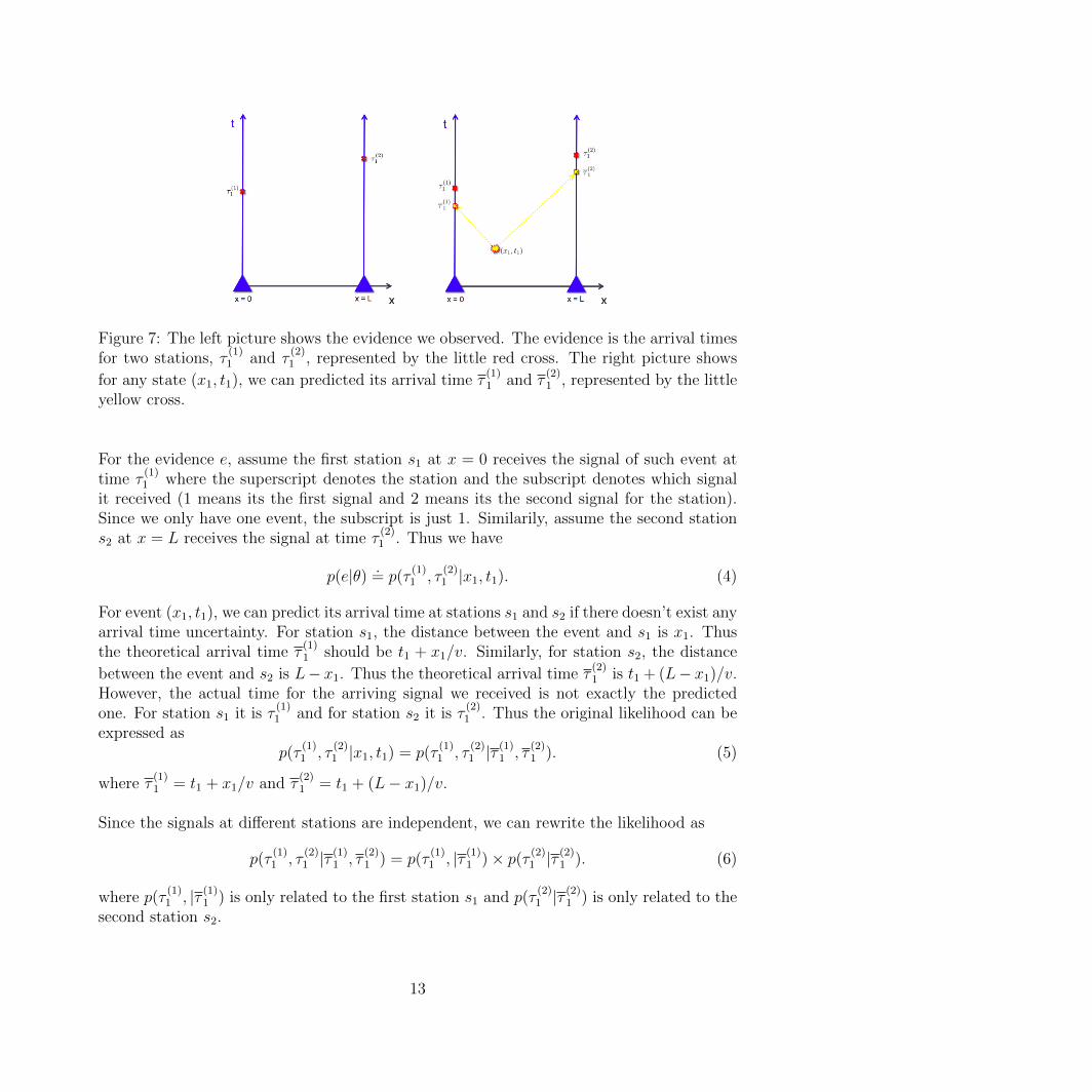
Figure 7: The left picture shows the evidence we observed. The evidence is the arrival timesfor two stations, τ
(1)1 and τ
(2)1 , represented by the little red cross. The right picture shows
for any state (x1, t1), we can predicted its arrival time τ(1)1 and τ
(2)1 , represented by the little
yellow cross.
For the evidence e, assume the first station s1 at x = 0 receives the signal of such event attime τ
(1)1 where the superscript denotes the station and the subscript denotes which signal
it received (1 means its the first signal and 2 means its the second signal for the station).Since we only have one event, the subscript is just 1. Similarily, assume the second stations2 at x = L receives the signal at time τ
(2)1 . Thus we have
p(e|θ) .= p(τ
(1)1 , τ
(2)1 |x1, t1). (4)
For event (x1, t1), we can predict its arrival time at stations s1 and s2 if there doesn’t exist anyarrival time uncertainty. For station s1, the distance between the event and s1 is x1. Thusthe theoretical arrival time τ
(1)1 should be t1 + x1/v. Similarly, for station s2, the distance
between the event and s2 is L− x1. Thus the theoretical arrival time τ(2)1 is t1 + (L− x1)/v.
However, the actual time for the arriving signal we received is not exactly the predictedone. For station s1 it is τ
(1)1 and for station s2 it is τ
(2)1 . Thus the original likelihood can be
expressed asp(τ
(1)1 , τ
(2)1 |x1, t1) = p(τ
(1)1 , τ
(2)1 |τ
(1)1 , τ
(2)1 ). (5)
where τ(1)1 = t1 + x1/v and τ
(2)1 = t1 + (L− x1)/v.
Since the signals at different stations are independent, we can rewrite the likelihood as
p(τ(1)1 , τ
(2)1 |τ
(1)1 , τ
(2)1 ) = p(τ
(1)1 , |τ (1)1 )× p(τ (2)1 |τ
(2)1 ). (6)
where p(τ(1)1 , |τ (1)1 ) is only related to the first station s1 and p(τ
(2)1 |τ
(2)1 ) is only related to the
second station s2.
13

Since we model the actual arriving signal recorded by station using a Gaussian distribu-tion, we can calculate p(τ
(1)1 , |τ (1)1 ) and p(τ
(2)1 |τ
(2)1 ) as below:
p(τ(1)1 , |τ (1)1 ) = N (τ
(1)1 , τ
(1)1 , σ) = 1√
2πσexp(− (τ
(1)1 −τ
(1)1 )2
2σ2 )
p(τ(2)1 , |τ (2)1 ) = N (τ
(2)1 , τ
(2)1 , σ) = 1√
2πσexp(− (τ
(2)1 −τ
(2)1 )2
2σ2 ).(7)
Thus, the likelihood is
p(e|θ) =1√2πσ
exp(−(τ(1)1 − τ
(1)1 )2
2σ2)× 1√
2πσexp(−(τ
(2)1 − τ
(2)1 )2
2σ2).
It can be expressed as
p(e|θ) =2∏
k=1
1√2πσ
exp(−(τ(k)1 − τ
(k)1 )2
2σ2). (8)
where k is the index for the station.
3.2.2 Likelihood for multiple events
Now we generalize to multiple events. Suppose we have n events, each described as (xi, ti)for i = 1, . . . , n. For the first station s1, the arrival times of the signals it receives are(τ
(1)1 , . . . , τ
(1)n ). For the second station s2, the arrival times are (τ
(2)1 , . . . , τ
(2)n ). Note that the
subscript i just means the i-th arrival time for a particular station. It doesn’t correspond toevent i.
Then, the likelihood can be expressed as
p(e|θ) =2∏
k=1
N∏i=1
1√2πσ
exp(−(τ(k)i − τ
(k)i )2
σ2) (9)
where k is the index for the station and i is the index for the events.
Note that when the number of events increases, there may exist more than one probablesolution. In fact, as the dimension our state increases, there will occur more local modes.High dimension is hard to visualize, let’s just use the two events case as an example. SeeFig. 8
14

Figure 8: Use two events in the1D model as an example that we have more than one solutionfor given evidence. Both yellow states and blue hollow states can give the same observation.Thus we say that we have two modes.
3.3 Arrival time uncertainty
It is obvious that the arrival time uncertainty, σ, is a crucial parameter because it will af-fect the posterior probability distribution. If σ is large then the peaks of the optima in theposterior will be quite broad, while for small σ the peaks in the posterior will be narrow.
This is referred to Fig. 9:
Figure 9: The left part is the model with a large arrival time uncertainty while the rightpart is the model with a small uncertainty.
We can see the model with a small arrival time uncertainty will have a quite sharp posteriorprobability distribution. Thus the slope is very small for most of the region. We say this isa fine version of the model compared to the coarse version model.
15

3.4 Proposal move
In the previous section, we introduced both the coarse and fine versions of the model , aswell as the calculation of likelihood. In this section we need to figure out the proposal movesso that we can implement our parallel tempering algorithm.
We have two kinds of proposal moves. The first one is a normal move that changes theposition of the state in one chain. The second is called a swap move that can switch thestate between the coarse and fine chain. In this section we use “state” to denote the state inone chain, and use “parallel state” to denote the combination of states from different chains.
3.4.1 Normal move
In this 1D case, our state space is (x, t)-space. Suppose we propose a new state using aGaussian distribution:
q(θ → θ′) = q(x, t→ x′, t′)
= N (x|x′, σpps x) N (t|t′, σpps t) (10)
Where σpps x and σpps t are the standard deviations. It shows how much each move makesthe new state deviate from the original.
This is reasonable and is symmetric. So q(θ → θ′) = q(θ′ → θ). Then, the acceptancerate can be expressed as:
r(θ → θ′) = min
(1,
Π(θ)q(θ → θ′)
Π(θ′)q(θ′ → θ)
)= min
(1,
Π(θ)
Π(θ′)
)(11)
Now, let’s run the MH algorithm in one chain first as an example.
Figure 10: An example of MH algorithm. Suppose we have two events with [x1, t1] =[0.17, 0.13] and [x2, t2] = [0.49, 0.38]. We can see the state will jump from an random initialstate to the actual state. And finally converge under the posterior probability distribution.
16

We can see that the initial state is far away from the peak of target distribution. Then itmoves to the peak gradually and finally the sample distribution will converge to the targetdistribution.
In our model we assume the number of events is fixed. When the number of events isunsure, this number becomes a parameter of our state. Then, we will include birth anddeath moves in the proposal, which allow the dimension of state to vary during the MHalgorithm (Oh, Russell, & Sastry, 2004; Green & Hastie, 2009).
3.4.2 Swap move
Now let’s consider the parallel state (θ1, θ2) where θ1 is the state in coarse chain and θ2 isthe state in fine chain. Thus, for the proposal distribution of swap move we have
q(θ1, θ2 → θ′1, θ′2) =
{1 if θ1 = θ′2, θ2 = θ′10 otherwise
(12)
Where the parameters, θ1, in coarse chain are the same as the parameters, θ′2, in the finechain. Parameters, θ2, in the fine chain are the same as the parameters, θ′1, in the coarsechain.
Since it is symmetric we can rewrite the acceptance rate as
r(θ1, θ2 → θ′1, θ′2) = min
(1,
Π(θ1, θ2)q(θ1, θ2 → θ′1, θ′2)
Π(θ′1, θ′2)q(θ
′1, θ′2 → θ1, θ2)
)= min
(1,
Π(θ1, θ2)
Π(θ′1, θ′2)
)(13)
Where Π(θ1, θ2) = Π(θ1) Π(θ2) is the probability of the parallel state is the product of theprobability of those states in each chain.
In our algorithm, we run two Markov chains simultaneously. The swap move is only usefulwhen the state in the coarse and fine chains both reach the mode. Thus, the swap moveshould be rare. Most of the proposal moves should be the normal move which change theposition of the state in each chain.
Thus, for each step of MH algorithm, we say that we have a probability of rn = 0.99that we choose a normal move for both the coarse and fine chain, and a probability of 1− rnthat we choose a swap move. rn is a parameter we can adjust during our algorithm.
3.5 Results
In reality, we usually draw log probability of the state versus step to observe its convergencebehavior. The state is usually high dimensional, so we draw one parameter of the state ver-sus the step. We can see that the parameter will converge to and jump between those modes.
17

In our program, we set the length scale L = 1, time scale T = 1, velocity v = 1, stan-dard deviation of arrival time uncertainty σcoarse = 0.2 for coarse chain and σfine = 0.05 forfine chain. The standard deviation of proposal distribution is σpps x = σpps t = 0.02
We set our actual state to be (x1, t1) = (0.3, 0.5), (x2, t2) = (0.7, 0.5), thus our targetdistribution has two modes.
First, we only run the fine chain. We run 50000 steps and plot the state parameter againstthe step:
Figure 11: This picture shows state parameter v.s. steps for fine chain with σ = 0.05. Inthis case, it is x1 v.s. steps. We also have t1, x2, t2 v.s. steps but we don’t draw it here sincethe parameters of one of the events are already enough to show the result. From the picturewe see that for the fine chain, it is rare for one state to jump between modes. In 10000 stepsthere are only two jumps.
From the picture above we can see that if we run standard MCMC, the frequency for a statetransferring between different modes is very slow.
Then we run the parallel tempering program. The results are listed below
18
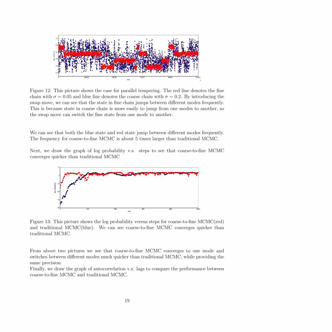
Figure 12: This picture shows the case for parallel tempering. The red line denotes the finechain with σ = 0.05 and blue line denotes the coarse chain with σ = 0.2. By introducing theswap move, we can see that the state in fine chain jumps between different modes frequently.This is because state in coarse chain is more easily to jump from one modes to another, sothe swap move can switch the fine state from one mode to another.
We can see that both the blue state and red state jump between different modes frequently.The frequency for coarse-to-fine MCMC is about 5 times larger than traditional MCMC.
Next, we draw the graph of log probability v.s. steps to see that coarse-to-fine MCMCconverges quicker than traditional MCMC
Figure 13: This picture shows the log probability versus steps for coarse-to-fine MCMC(red)and traditional MCMC(blue). We can see coarse-to-fine MCMC converges quicker thantraditional MCMC.
From above two pictures we see that coarse-to-fine MCMC converges to one mode andswitches between different modes much quicker than traditional MCMC, while providing thesame precision.Finally, we draw the graph of autocorrelation v.s. lags to compare the performance betweencoarse-to-fine MCMC and traditional MCMC.
19

Figure 14: This picture shows the autocorrelation v.s. lags for coarse-to-fine MCMC(red) andtraditional MCMC(blue). We can see the autocorelation of coarse-to-fine MCMC convergesto zero much quicker than traditional MCMC, which means the state is easier to jump toother positions after a long enough steps.
The picture above shows autocorrelation of state parameter v.s. lags. When lag increases,the autocorrelation approaches to zero. This means that a state’s position is unrelated to itsposition after enough steps. We can see that, for coarse-to-fine MCMC, it converges quickerthan traditional MCMC.
These results show that coarse-to-fine MCMC performs better.
20

4 1D discrete model
4.1 Insight of introducing discrete model
In the previous model, adjusting the arrival time uncertainty controls how coarse our con-tinuous model is. Now, we introduce the discrete model which is closer to the signal-basedsystem.
Suppose each station has a resolution and it can not give the precise arrival time in aparticular time period. But it can tell you how many signals it received during that period.When the resolution is low, we define it as “coarse”. Compared to the continuous model,arrival time uncertainty as a measure of “coarseness” is just an analogy for discretization.Similarly, when the resolution is low, it corresponds to a fine version model.
Figure 15: Suppose now we have discretized model. The left part corresponds to a coarsechain while the right part corresponds to a fine chain.
By introducing this new parameter resolution, we can apply coarse-to-fine MCMC withoutmodifying the seismic model.
4.2 Discrete model description
4.2.1 Time scale for stations
In order to introduce the discrete model, let’s first consider the time scale for event. In thecontinuous model, the time scale for the events is [0, T ], thus the time scale for the stationis [0, T + L/v] = [0, Ts].
4.2.2 Station resolution
In the continuous case, the arrival time recorded by each station is a real number. However,in the discrete case, we suppose each station has finite resolution and the actual arrival timecan not be very precise. But it can tell you how many signals it received in this period. Wesay the station has high resolution when the time period is short and low resolution when
21

the time period is long.
For example, suppose the time scale of the station is [0, 1]. Then if the resolution of thestation is 0.1, we have 10 possible choices for the arrival time. If the resolution is 0.01 thenwe have 100 choices, and similarly, 1000 choices for resolution 0.001.
After we set the station resolution, we can see the arrival time of the events are discretized.It has only finite states. Suppose the resolution, res, of the station is Ts/5, thus the timeperiods are [0, Ts/5], [Ts/5, 2Ts/5], [2Ts/5, 3Ts/5], [3Ts/5, 4Ts/5], [4Ts/5, Ts/5]. We representit as τ1, τ2, τ3, τ4, τ5. Remember that in discrete model τ represents a particular time periodinstead of a precise time point.
4.2.3 Signal amplitude
Next, let’s assume each event contains some units of energy, represented by ene. When thewave of event arrives at the station, the average magnitude of the signal is proportional toene/res. This is intuitive since, if the resolution is fine, then the station will receive thisenergy in a smaller time period and enhance its magnitude level.
As an example, for station s1, suppose one arriving signals come during time period τ2and two signals come during time period τ4. The signal received should be
signal(1) = [0,ene
res, 0, 2
ene
res, 0]. (14)
The signal can be illustrated below:
Figure 16: Ts is the time scale for the station. Suppose the resolution is Ts/5. Then, thegreen dotted line represents the signal the station received when τ2 receives one arrivingsignal and τ4 receives two arriving signals.
4.2.4 Noise
Because seismic signals are noisy, we include noise in our model. In addition, by includingnoise, we can directly apply a Gaussian distribution to calculate the likelihood, which can
22

avoid unrealistic delta functions.
Suppose we have noise in our signal with mean µ and variance σnoise. For each period,τi, the amplitude level of noise, noi, is under N (µ, σnoise).
Thus we can express the signal as the formula below when we consider noise:
signal(1) = [no1, no2 +ene
res, no3, no4 + 2
ene
res, no5]. (15)
The signal can be illustrated below:
Figure 17: The green dotted line is the signal without noise, while the blue solid line is theactual signal when we consider noise.
Thus, for a particular resolution, our observation is one such signal for every station. Wehope to infer the actual events.
4.3 Calculation of likelihood
4.3.1 Likelihood for only one event
For simplicity, let’s consider the case with only one event first. The evidence for one stationis like
Figure 18: The actual signal above shows the case of only one events. Notes that in eachperiod, τi, the magnitude level is non-zero because noise exists.
23

We express this signal as si(k) = [si(k)1 , . . . , si
(k)5 ] where k represents the index of station.
Then, for any given state (x1, t1), the likelihood can be expressed as
p(e|θ) = p(si(1), si(2)|x1, t1) (16)
For a particular state (x1, t1), we can predicted its arrival time for a given station, τ(k)1 ,
where k represents the index of the station. Suppose τ(k)1 arrives in τ2. In this case, it can
illustrated in the picture below:
Figure 19: For any given state we can predict its arrival time presented by the little redcross. Due to the arrival time uncertainty it may corresponds to multiple predicted signalswith particular weights.
Due to the arrival time uncertainty, these arrival times are located in adjacent time periodswith some set probability. Though it should be located in τ2 theoretically, it can also belocated τ1 and τ3.
Thus, we need to calculate the weights for predicted arrival times being located in eachparticular τi. Such weight in fact is the integral of a Gaussian function in each time period.In the example above, we assume the probability that τ1 receives a signal is w1, similarly theprobabilities for τ2 and τ3 are w2 and w3. Because the Gaussian distribution has an infinitlylong tail, we cut the tail at two deviations to simplify the calculation. Remember that weneed to do renormalization for wi during the calculation. After that we can see for each
24

predicted signal we have a weight wi that corresponds to it:
wi =
∫τi
N (t|τ (k)1 , σ)dt. (17)
Where τ(k)1 is the predicted arrival time.
For each wi (i = 1, 2, 3), suppose the predicted signal is pred si(k,i), then the likelihoodcan be expressed as
p(e|θ) =3∑i=1
wi × pi(si(1), si(2)|pred si(1),i, pred si(2),i) (18)
Where i denotes different cases and pi denotes the likelihood for each case. Since the signalsin different stations are independent, we can rewrite the likelihood as:
p(e|θ) =3∑i=1
wi × p(1)i (si(1)|pred si(1),i)× p(2)i (si(2)|pred si(2),i)
=3∑i=1
wi
2∏k=1
p(k)i (si(k)|pred si(k),i) (19)
Figure 20: For a given state and station we can calculate its wi and likelihood pi for eachcase i. The likelihood is the sum for each case,
∑iwi × pi.
25

Next, for each case wi (i = 1, 2, 3), we can compare the actual signal with the predictedsignal and then calculate its likelihood pi. From previous part we know the signal consistsof 5 parts since the resolution is Ts/5. Thus for any actual signal si(k) and predicted signalpred si(1),i, we have:
si(k) = [si(k)1 , . . . , si
(k)5 ] (20)
pred si(k),i = [pred si(k),i1 , . . . , pred si
(k),i5 ] (21)
Since the magnitude level in different periods are independent, and in each period, the dif-ference of the actual magnitude level and predicted magnitude level is due to the uncertaintyof noise, we know the smaller difference between the actual magnitude level and predictedactual level, the higher probability that this prediction is true.
Thus, we can express each likelihood as
p(k)i (si(k)|pred si(k),i) =
5∏j=1
N (si(k)j , pred si
(k),ij , σnoise). (22)
Finally, the full likelihood is expressed as:
p(e|θ) = p(si(1), si(2)|x1, t1)
=3∑i=1
wi
2∏k=1
5∏j=1
N (si(k)j , pred si
(k),ij , σnoise). (23)
Where i denotes any probable cases, k denotes different stations, j denotes to different timeperiod for the station signal.
This is only for the state with one event, thus i is relatively small. Later we will see that whenthe number of events increase, the probable cases for the state will increase exponentially.
4.3.2 Likelihood for multiple events
The likelihood for multiple events are similar. Use two events as an example.
Suppose for some state, two predicted arrival time locates in τ2 and τ4. Due to the ar-rival time uncertainty, for the first arrival, it can be located either in τ1, τ2, τ3. And for thesecond arriving, it can be located either in τ3, τ4, τ5. Thus we have 3 × 3 = 9 cases whichcan be shown in the picture below.
26

Figure 21: The picture above shows 9 cases of probable predicted signals for two events stateand compare it with the actual signal. For the same column, the first arriving signal arealways in the same τ , while different row means the second arriving signal are in differentτ . Similarily, for the same row, the second arriving signal are always in the same τ , whiledifferent columns mean that the first arriving signal are in different τ . The green dotted lineis predicted signal and blue solid line is actual signal. The resolution of the station is Ts/5.
From the above picture, we can see in most of the cases (except w5), the overlap of thepredicted signal and actual signal is quite small. The most probable case is w5. The casesfar away from w5 have little probability.
Thus, the likelihood is
p(e|θ) =3∑i=1
wi
2∏k=1
5∏j=1
N (si(k)j , pred si
(k),ij , σnoise). (24)
It is the same as the likelihood in the case of a single event, while wi represents all the caseshere.
27

4.4 Proposal move
In previous chapter, we introduced the proposal move for the continuous model. It is similarfor the discrete model. (N. Arora et al., 2010)
For a normal moveq(θ → θ′) = N (x, x′, σpps x) N (t, t′, σpps t). (25)
Thus, the acceptance rate is
r(θ → θ′) = min
(1,
Π(θ)
Π(θ′)
). (26)
For a swap move
q(θ1, θ2 → θ′1, θ′2) =
{1 if θ1 = θ′2, θ2 = θ′10 otherwise .
(27)
Thus the acceptance rate is
r(θ1, θ2 → θ′1, θ′2) = min
(1,
Π(θ1, θ2)
Π(θ′1, θ′2)
)(28)
4.5 Results
For the discrete model, the results are quite similar with those of the continuous model. Inour discrete model, we set the length scale L = 1, time scale T = 1, velocity v = 1, standarddeviation of arrival time uncertainty σ = 0.1. The resolution of station for coarse model is0.4 and the resolution for fine model is 0.2. The standard deviation of proposal distributionis σpps x = σpps t = 0.02
We set our actual state to be (x1, t1) = (0.3, 0.5), (x2, t2) = (0.7, 0.5), thus our targetdistribution has two modes. It is the same as the continuous model.
First, we only run the fine chain. We run 50000 steps and draw state parameter v.s stepdiagram.
28

Figure 22: This picture shows state parameter v.s. steps for fine chain with res = 0.2. Wesee that for the fine chain, it is rare for one state jumping between different modes. In 10000steps there is only one jump.
Thus, we know that, in standard MCMC, the frequency for a state transferring betweendifferent modes is low.
Then, we run the parallel tempering program.
Figure 23: This picture shows the case for parallel tempering. The red line denotes thefine chain with res = 0.2 and the blue line denotes the coarse chain with res = 0.4. Byintroducing the swap move, we can see that the state in the fine chain jumps between differentmodes frequently.
We can see that both the blue states and red states jump between different modes frequently.
Finally, we draw the graph of autocorrelation v.s. lags to compare the performance be-tween coarse-to-fine MCMC and traditional MCMC.
29

Figure 24: Autocorrelation v.s. lags for coarse-to-fine MCMC(blue) and traditionalMCMC(red). The autocorelation of coarse-to-fine MCMC converges to zero much quickerthan traditional MCMC.
Generally speaking, the results for the discrete model are similar to the results from thecontinuous model. We can say that coarse-to-fine MCMC has better performance in bothof these models. It provides shorter convergence time as well as higher frequency jumpsbetween modes.
30

5 Conclusion
The coarseness of a chain is crucial for the behavior of sampling in MCMC. Coarse chainsprovide more opportunities to jump between different modes. While fine chains give moreprecise solution for a particular mode.
Coarse-to-fine MCMC combines the advantage of both of them. It mixes the chains withdifferent coarseness and helps the state in fine chain to jump between different modes asquickly as those states in coarse chain. It gives very precise solutions for one mode, andexplores different modes at the same time.
In the previous examples, we compared how states jump between mode in coarse-to-fineand traditional MCMC. We conclude that coarse-to-fine MCMC has a higher frequency forstate transferring between different modes. We also compared log probability and autocor-relation to confirm that. Thus, in order to achieve the same result, coarse-to-fine MCMCrequires fewer steps. The efficiency would be enhanced for such problems.
31

References
Amit, Y., Geman, D., & Fan, X. (2004). A coarse-to-fine strategy for multiclass shapedetection. Pattern Analysis and Machine Intelligence, IEEE Transactions on, 26 (12),1606–1621.
Andrieu, C., De Freitas, N., Doucet, A., & Jordan, M. I. (2003). An introduction to MCMCfor machine learning. Machine Learning , 50 (1-2), 5–43.
Arora, N., Russell, S. J., Kidwell, P., & Sudderth, E. B. (2010). Global seismic monitoringas probabilistic inference. In Advances in neural information processing systems (pp.73–81).
Arora, N. S., Russell, S., & Sudderth, E. (2013). NET-VISA: Network processing verticallyintegrated seismic analysis. Bulletin of the Seismological Society of America, 103 (2A),709–729.
Bouvrie, J., & Maggioni, M. (2012). Efficient solution of markov decision problems withmultiscale representations. In Communication, control, and computing (allerton), 201250th annual allerton conference on (pp. 474–481).
Efendiev, Y., Hou, T., & Luo, W. (2006). Preconditioning Markov chain Monte Carlosimulations using coarse-scale models. SIAM Journal on Scientific Computing , 28 (2),776–803.
Efendiev, Y., Jin, B., Michael, P., & Tan, X. (2015). Multilevel Markov chain Monte Carlomethod for high-contrast single-phase flow problems. Communications in Computa-tional Physics , 17 (01), 259–286.
Fleuret, F., & Geman, D. (2001). Coarse-to-fine face detection. International Journal ofComputer Vision, 41 (1-2), 85–107.
Geyer, C. J. (1991). Markov chain Monte Carlo maximum likelihood.Green, P. J., & Hastie, D. I. (2009). Reversible jump MCMC. Genetics , 155 (3), 1391–1403.Higdon, D., Lee, H., & Bi, Z. (2002). A Bayesian approach to characterizing uncertainty
in inverse problems using coarse and fine-scale information. Signal Processing, IEEETransactions on, 50 (2), 389–399.
Moore, D. A., Mayeda, K. M., Myers, S. M., Seo, M. J., & Russell, S. J. (2012). Progress insignal-based Bayesian monitoring. Proceedings of the 2012 monitoring research review:ground-based nuclear explosion monitoring technologies, LA-UR-12-24325 , 263–273.
Oh, S., Russell, S., & Sastry, S. (2004). Markov chain Monte Carlo data association forgeneral multiple-target tracking problems. In Decision and control, 2004. cdc. 43rdieee conference on (Vol. 1, pp. 735–742).
Pedersoli, M., Vedaldi, A., & Gonzalez, J. (2011). A coarse-to-fine approach for fast de-formable object detection. In Computer vision and pattern recognition (cvpr), 2011ieee conference on (pp. 1353–1360).
32