coalition governments, cabinet size, and the common …
TRANSCRIPT

ISSN: 1439-2305
Number 165 – July 2013
COALITION GOVERNMENTS, CABINET
SIZE, AND THE COMMON POOL
PROBLEM: EVIDENCE FROM THE
GERMAN STATES
Thushyanthan Baskaran

Coalition governments, cabinet size, and the common pool
problem: evidence from the German States
Thushyanthan Baskaran∗
University of Goettingen
Abstract
The theoretical literature on common pool problems in fiscal policy suggests that
government fragmentation increases public expenditures. In parliamentary regimes,
the fragmentation hypothesis refers to (i) coalition governments and (ii) cabinet size.
This paper explores the effect of coalition governments and cabinet size on public ex-
penditures with panel data covering all 16 German States over the period 1975-2010.
Identification is facilitated by the large within-variation in the incidence of coalition
governments and the size of the cabinet in the German States. In addition, I exploit
a feature of state electoral laws to construct a credible instrument for the likelihood
of coalition governments.
Keywords: Government fragmentation, common pool problems, coalition government,
cabinet size, public expenditures
JEL codes: D78, H61, H72
∗Thushyanthan Baskaran, Department of Economics, University of Goettingen, Platz der GoettingerSieben 3, 37073 Goettingen, Germany, Tel: +49(0)-551-395-156, Fax: +49(0)-551-397-417.

1 Introduction
What determines the size of the public sector? The literature on this question can be
classified along three lines. The traditional strand relates public expenditures to underlying
economic trends. A famous contribution is Wagner’s Law, according to which public sector
size increases disproportionately with economic development (Wagner, 1911). This theory
perceives the government as a benevolent planner who responds optimally to developments
that are outside of its control. It is, however, contentious whether governments are truly
benevolent. Perhaps to emphasize their skepticism toward the benevolence assumption,
Brennan and Buchanan (1980) go as far as to model the government as a Leviathan who
is only interested in revenue maximization. In the Leviathan-framework, the size of the
public sector is explained by the extent to which the fiscal constitution is capable to limit
the ability of the government to over-tax citizens.1
In reality, governments are neither completely benevolent nor do they behave exclusively
as Leviathans. The third strand of the literature focuses on the role of politics and applies
neoclassical tools to model political decisions as the outcome of the interactions of self-
interested and rational agents who respond optimally to the incentives they face. Within
this political economics literature, the seminal contributions of Weingast et al. (1981) and
Shepsle and Weingast (1981) on common pool problems in policy making suggests that
government fragmentation is one important determinant of public expenditures.
In countries with parliamentary regimes, the term government fragmentation refers to
(i) the number of parties and (ii) the number of ministers represented in the government.2
The two variants of government fragmentation can result in common pool problems if the
1For example, it follows from the Leviathan model that public expenditures will decline in the degreeof fiscal decentralization. The reason is that fiscal decentralization will result in tax competition, whichwill diminish the ability of the government to over-tax citizens.
2 The original model was developed for US-style legislatures and usually refers to the size of thelegislature. Another variant of government fragmentation in countries with presidential regimes refers tosituations with divided government, i. e. where the executive and the legislature are controlled by differentparties (Alt and Lowry, 1994).
1

benefits of public expenditures can be targeted to well-defined constituencies whereas the
costs are shared equally by all members of the government. The reasoning is as follows.
Each member of the government has to weigh the benefits of public expenditures against
their cost. If expenditures can be targeted, the constituency of a government member fully
internalizes the benefits. The cost associated with public expenditures is the political price
that the government has to pay for either higher taxes or more debt. If the cost for targeted
expenditures is shared among all members of the government, each individual member only
pays a small fraction. Consequently, overall demand for public expenditures will increase in
the number of government members. And given that “government members” can be defined
either in terms of parties or in terms of ministers, the fragmentation hypothesis predicts
that expenditures will increase in the number of parties represented in the government and
the size of the cabinet.
A large empirical literature attempts to test how coalition governments and cabinet
size relate to public expenditures. The relevant studies can be distinguished by whether
they use cross-country or sub-national data. Notable cross-country studies are Roubini
and Sachs (1989a,b), Edin and Ohlsson (1991), De Haan and Sturm (1997), Perotti and
Kontopoulos (2002), Woo (2003), and Bawn and Rosenbluth (2006). While there are
some conflicting results3, this strand of the literature tends to conclude that both coalition
governments and large cabinets exacerbate the common pool problem and cause either
more spending or higher deficits.
However, one problematic feature of the cross-country studies is that they have to cope
with a large degree of heterogeneity. It is difficult to fully account for the cross-country
heterogeneity by means of control variables. A recent literature attempts to address the
heterogeneity problem by using data at the sub-national level. Ashworth and Heyndels
(2005), for example, show that in Flemish municipalities, coalition governments and large
3For example, De Haan and Sturm (1997) find no evidence for the fragmentation hypothesis.
2

cabinets are in general associated with higher spending. Le Maux et al. (2011) find for
French Departments that the number of parties in the ruling coalition is positively related
to social expenditures. Borge (2005) concludes for Norwegian municipalities that less
fragmented local councils lead to smaller deficits.
While these studies use data at the local level, Schaltegger and Feld (2009) use data
at the level of the Swiss Cantons. Compared to municipalities, the Swiss cantons have
significant political autonomy and are responsible for a large share of total public expen-
ditures. Schaltegger and Feld (2009) find that public spending increases in the size of
the cabinet while the effect of coalition governments is ambiguous. One problematic fea-
ture of their study is, however, that over-time variation in their coalition and cabinet size
variables is limited. The small within-variation in their data forces them to base their
conclusions primarily on the variation between cantons. Consequently, there could remain
unobserved factors that influence both public expenditures and government fragmentation
simultaneously.
I study in this paper whether coalition governments and large cabinets cause larger
public spending with panel data covering all 16 German States over the period 1975-2010.4
As the Swiss Cantons, the German States offer an excellent opportunity to investigate the
effects of fragmented governments at a powerful and fiscally important tier of government.
The German States have similar political and legal systems, a common history, and close
linguistic and cultural ties. Because of the relative homogeneity of its states, the German
federation can serve as a natural laboratory. But unlike the Swiss Cantons, the German
States exhibit large within-variation in the incidence of coalition governments and the
4 In contrast to Schaltegger and Feld (2009), I focus on whether a state government is formed by asingle party or by a coalition of parties, but not on the size of the coalition. The reason is that stategovernments in Germany are typically formed by either a single party or by a coalition of two parties.Coalitions with three parties are extremely rare and coalitions with more than three parties were neverformed.
3

number of cabinet ministers, allowing the identification of the public spending effects of
coalition governments and large cabinets by means of fixed effects regressions.
To further account for possible endogeneity, I exploit a feature of the electoral laws
in all states that relates vote shares to seats in state parliaments in a non-linear fashion
to construct a compelling instrument for the likelihood of coalition governments. In a
nutshell, every state has a so called “five-percent hurdle”. Only parties that receive more
than five percent of the votes are entitled to seats in parliament. Any seats to which parties
with less than five percent of the votes would in principle be entitled to are distributed
among the parties that actually manage to enter the state parliament. This feature of the
electoral law has the consequence that the fewer parties enter the state parliament, the
easier it is to form a single-party government for the biggest party because the probability
of having more than 50% of the seats is inversely related to the number of parties in
parliament. At the same time, the number of parties in parliament has no obvious direct
effect on spending. Consequently, this variable can serve as a valid and strong instrument
for coalition governments.
The link between coalition governments and public deficits in the German states has
been previously analyzed by Jochimsen and Nuscheler (2011). As German States have
no tax autonomy (see below), borrowing and expenditures are closely linked. However,
since the fragmentation hypothesis is only one of many hypotheses that Jochimsen and
Nuscheler (2011) investigate, it is only cursorily explored. In particular, it is unclear
whether their result that coalition governments spend more than single party governments
is robust. In contrast, I focus exclusively on the fragmentation hypothesis which allows for
a more thorough analysis. Indeed, my results with respect to the fiscal effects of coalition
governments contradict the findings in Jochimsen and Nuscheler (2011).
The link between the structure of the cabinet and fiscal policy has been previously
explored for Germany as well. A relevant contribution is Jochimsen and Thomasius (2012)
4

who study how characteristics of the finance minister relate to deficits. Yet, the overall size
of the cabinet is neglected in their paper. Further studies exploring the political economy
of fiscal policy in the German States, albeit with a different focus than the fragmentation
hypothesis, are Seitz (2000), Galli and Rossi (2002), and Pitlik et al. (2005).
2 The fiscal and political landscape in the German
States
Germany consists of sixteen federal states: eleven West-German and five East-German (see
Figure 1 for a map).5 The fiscal constitution grants all states significant spending but only
minuscule tax autonomy. Each of the states can borrow and spend according to its own
discretion, while rates and bases for most taxes are the same throughout the federation.
Variation in state level taxation only exists for some unimportant taxes.
The federal constitution defines a wide set of public goods which have to be provided
by the sub-national tier. States are expected to finance all stages of education, cultural
affairs, the police, and many other public goods.6 The policy areas for which the states are
responsible make up more than half of public spending in the German federation. While
there are some federal mandates defining minimum levels for the state public goods, states
can in general decide autonomously on expenditures (Seitz, 2008). Figure 1 shows that
the states use their expenditure autonomy extensively. The average real expenditures per
capita during the 1975-20010 period in Berlin, Bremen, Hamburg, or the East-German
states was almost twice as high as in Bavaria and Lower-Saxony. There is also signifi-
5The state of Berlin is somewhat of a hybrid because it was formed in 1991 by merging the westernwith the eastern part of the city. In the following, I treat Berlin as a West-German State.
6The sub-national tier consists of states and different types of localities. However, the localities arelegally subordinate and accountable to the states (Kipke, 2000). In particular, the federal constitutiondefines local finances as part of state finances (Art. 106 Abs. 9 GG). All fiscal variables discussed inthe following (notably state expenditures and revenues per capita) are consolidated between states andlocalities.
5

cant amount of over-time variation in state spending as suggested by Figure 2. Average
expenditures per capita in the West-German states increased until 1990, then spiked dra-
matically, presumably because of the need to fund the German unification. Thereafter,
a slow decline in expenditures per capita can be observed in the West-German States
until the outbreak of the financial crisis in late 2007. In East-Germany, expenditures in-
creased until the mid-nineties, again presumably because of the need to modernize public
infrastructure and delays in reducing the number of public employees in the aftermath of
unification (Reichard, 2001). From the mid-nineties onward, however, expenditures per
capita have been on a downward trajectory in East-Germany. By 2010, they had declined
below the level of the West-German states.
Politically, the German States are parliamentary democracies. Each state has a unicam-
eral parliament elected by its residents.7 Elections to the state parliament are governed by
electoral laws that are, while not identical, very similar throughout the federation. Most
importantly, all states have a so called “five-percent hurdle” that limits the number of
parties that may enter parliament. This hurdle – introduced in order to avoid a repetition
of the massive party fragmentation in the Reichstag during the Weimar Republic and the
ensuing difficulties in forming a government with sufficient parliamentary support– implies
that only parties which receive at least five percent of the votes will get seats in the parlia-
ment.8 This feature of the electoral system ensures that parties that are allowed to enter
parliament receive a larger share of seats than would be warranted by the vote share, which
7Bavaria’s parliament had a second chamber, the Senate, until 1999. The Senate was abolished througha popular referendum because it was essentially powerless.
8There are two exceptions. Parties with less than five percent may enter the state parliament in somestates if some of their candidates win in their districts (the number of districts that have to be carried bythe party to enter parliament through this rule varies between states). This exception is fairly irrelevantand has hitherto only applied to one party, the PDS, and only at the federal level. At the state level, thePDS either easily passed the five-percent hurdle (in the East-German states) or did not win any directmandates (in the West-German states). There is also an exception for the party of the Danish minority(the SSW) in the state of Schleswig-Holstein. For this party, the five-percent hurdle is waived.
6

makes it easier to form a government with majority support in parliament. I discuss the
consequences of this feature of the electoral system in more detail in Section 6.
In 1975 there were three major parties both at the federal level and in each of the eleven
West-German States: the Christian Democratic Union (CDU), the Social Democratic Party
of Germany (SPD), and the Free Democratic Party (FDP). In general, the CDU is perceived
as culturally conservative (i. e. supporting “traditional” values) and moderately market-
oriented. The SPD is moderately left-leaning on economic and moderately liberal on
cultural issues. The FDP is culturally liberal and market-oriented with respect to its
economic policies. By 2010 the number of mainstream parties in the now unified Germany
had increased to five. In addition to the CDU, SPD, and FDP, the Green Party and a new
left-wing party (Party of Democratic Socialism (PDS), later renamed Die Linke) entered
the political scene.
The Green Party started to receive significant vote shares at the end of the seventies
by focusing on environmental and peace issues (recall that the cold war was still ongoing
at the time). It is moderately left-leaning on economic policies. Yet, its main support
base are civil servants rather than the working class. With respect to cultural issues, it is
generally perceived as very liberal.
By the mid-eighties and early nineties, the Green Party had entered most state parlia-
ments and was even part of some state governments as a coalition partner of the SPD. This
change in the German party system is reflected in Panel (a) of Figure 3.9 According to
9There is some ambiguity in determining the correct coding of the number of parties in parliament andother political variables in election years. The type of government, the size of the cabinet, and the numberof parties in parliament typically change after an election. The election dates, however, differ both betweenand within states. I apply the following rule: if an election in year t takes place after July 1th, I codethe political variables for year t according to the situation early in the year (since the old administrationhas governed more than half of the year). If the election takes place before July 1th, I code the politicalvariables according to the situation late in the year.For example, assume that the SPD has received more than 50% of the seats in an election in state i
in year t, so the next administration will be formed by the SPD. Assume furthermore that the currentadministration is a CDU-FDP coalition. If the election took place on or after July 1st, I code the coalitionvariable as 1. If the election took place before July 1th, I code the coalition variable as 0. I apply the same
7

this panel, the median number of parties in West-German state parliaments was three until
the mid-eighties. Then the median number jumps to four and remains there until the end
of the sample period, where it increases to five. The evolution of the average number of
parties in state parliaments, too, reflects the rise of the Green Party. This number remains
around three until the mid-eighties and then increases fairly steeply to four and remains
there until 2005. At the end of the sample period, the average number had increased to
five.
The other addition to the German party system during the 1975-2010 period was the
Party of Democratic Socialism (PDS). Unlike the Green Party, the PDS did not represent a
new political movement. Rather, it was the former ruling party of the German Democratic
Republic (GDR) – the Socialist Unity Party (SED)– that had reconstituted itself as the
PDS after the demise of the GDR in 1990. In 2007, the PDS merged with a West-German
Party called WASG and reconstituted itself as Die Linke. For simplicity, I will refer for
the remainder of this paper to Die Linke as PDS.
The importance of the PDS in East-Germany is implicitly reflected in Panel (b) of
Figure 3. According to this panel, the median number of parties in the East-German
state parliaments was five in the first half of the nineties. In the mid-nineties, the median
number dropped to three and remained there until the very end of the sample period, as
both the FDP and the Green Party found it increasingly difficult to collect sufficient votes
to enter parliament. The three parties that remained relevant in the East-German party
system were the CDU, the SPD, and the PDS. Only after 2005, things begun to change
with respect to both the average and median number of parties in parliament increasing
to five in 2010.
Figure 4 shows the average number of parties in the East- and West-German state
parliaments. This figure suggests that states differ in their openness toward smaller parties.
rule for the cabinet size variable, the parties in parliament variable, and the number of seats in parliamentvariable.
8
In Bavaria, the average number of parties represented in parliament was around three. In
states like Baden-Wuerttemberg, Berlin, and Bremen, the average number of parties was
over four during the 1975-2010 period.
The CDU and SPD are generally referred to as the “big” parties during the 1975-2010
period because they typically received between 30% to 40% of the votes in each election.10
The FDP and the Green Party are referred to as the “small” parties. The PDS is difficult
to classify along this dimension. In East-Germany, it was not uncommon for the PDS
to receive around 25% of the votes during the 1975-2005 period. It may therefore be
legitimately classified as a big party in the eastern part of Germany. In West-Germany,
however, the PDS never managed to get more than five percent of the votes until the very
end of the sample period (with the exception of Berlin).
The state government requires a majority in the parliament to govern effectively. Mi-
nority governments are therefore very rare and generally short-lived.11 As a rule, each of
the two big parties forms a single-party government if it receives more than 50% of the
seats. There have been some exceptions to this rule, but not in recent times. That is, a big
party with an absolute majority has sometimes invited a small party to join a coalition,
but the small parties have always declined to do so during the 1975-2005 period. One
example is Hesse after the elections of 2003 where the CDU gained an absolute majority
but nonetheless invited the FDP to join the cabinet. The FDP declined.
10By now, this characterization is probably too simple because the Green Party has in some states,most notably in Baden-Wuerttemberg, over-taken the SPD in terms of votes. Nevertheless, the generalperception is that the SPD is still the biggest left-wing party.
11Most minority governments are essentially caretaker governments that last only a few months be-fore new elections can be held. The only meaningful exceptions were the SPD-Green Party governmentin Saxony-Anhalt during 1994-1998 and the sole SPD government in Saxony-Anhalt during 1998-2002.These two governments had the implicit support of the PDS, even though it was not formally part of thegovernment. It might be argued that the sole SPD government in Saxony-Anhalt was in reality a coalitionwith the PDS in all but name. Moreover, there is theoretical work which suggests that in situations withminority governments, the opposition might play a decisive role for fiscal outcomes (Falco-Gimeno andJurado, 2011). However, (unreported) regression results with a redefined coalition variable that codesSaxony-Anhalt as having a coalition government during the 1998-2002 period are very similar to thosereported in the paper.
9

If one of the big parties has less than 50% of the votes in parliament, negotiations to
form a coalition government are held. The need to hold a new election because of the
inability to form a government almost never arises as the parties represented in parliament
can almost always agree on some type of coalition.12 A big party typically prefers to form
a coalition with a small party if they together can achieve a majority in parliament. If this
should not be possible, the two big parties usually form a coalition.13 Only in four cases,
coalition governments consisting of three parties have been formed (one big and two small
parties). Coalition governments consisting of more than three parties were never formed.
In principle, every party can form a government with any other party. In practice,
only certain types of coalition governments have been formed in the 1975-2010 period.
Figure 5 reports the relative frequencies of different types of (coalition and single-party)
governments. During the sample period, neither the CDU nor the FDP collaborated with
the PDS. In West-Germany, the SPD and the Green Party also refused to cooperate with
the PDS. (Berlin, however, is again an exception: the SPD did form a government with
the PDS there). Figure 5 also reveals some additional ideological patterns in coalition
formation. The CDU tends to form coalitions with the FDP whereas the SPD tends to
form coalitions with the Green Party, even though some coalitions between the SPD and
the FDP also took place. Only at the very end of the sample period, these patterns begun
to change slightly. In Hamburg, a coalition governments between the CDU and the Green
Party was formed in 2008, but it was only short-lived. Similarly, a CDU-Green Party-FDP
government was formed in 2010 in Saarland, but was soon dissolved as well.
Around half of all state governments in the 1975-2010 period have been formed by a
single party. The CDU has formed more single party governments than the SPD, but the
SPD has also managed to form a significant number of single party governments. Panel (a)
12However, Hesse after the election of 2008 is a recent example where new elections had to be calledbecause of the inability of the parties to form a stable government.
13In contrast to recent theoretical work on coalition formation, e. g. Bandyopadhyay and Oak (2008)and Tridimas (2011), coalition formation in Germany is thus straightforward.
10

in Figure 6 shows the number of state governments in West-Germany ruled by coalition
governments for each year between 1975-2010. Five of the eleven western states were ruled
by coalition governments in 1975. By 1980, their number had fallen to two and in 1985
even declined to one. Thereafter, there was a continuous increase in the number of coalition
governments. In 2003, eight states were governed by coalition governments. In 2005, the
number still stood at seven. In 2010, it had increased to ten. Panel (b) reports the number
of coalition governments during the 1991-2010 period in East-Germany. The eastern states
start out with four coalition governments. Their number declines to two around 2000. By
2010, however, their number had once again risen to five.
Figure 7 reports the relative frequency of coalition governments in each of the German
States. It reveals that all but one state have experienced both single-party and coali-
tion governments during the sample period. The only exception is Mecklenburg-Western
Pomerania, which was consistently ruled by a shifting set of coalition governments. On the
other hand, single-party and coalition governments were almost equally common in States
like North Rhine-Westphalia and Bremen. Overall, both Figure 6 and 7 confirm that
there is a significant amount of between and within-variation in the incidence of coalition
governments.
Once agreement on a government with a legislative majority has been reached between
the parties involved, the cabinet is formed. The process starts with the election of a
state prime minister by the state parliament. The state prime minister then appoints
his cabinet. In some states the cabinet has to be approved by the state parliament, but
this is only a formality. While the state prime minister is in theory free to choose the
cabinet members and the scope of the individual ministries, the parties involved in the
government have significant influence on the structure of the cabinet and the identity of
the ministers. There are some core ministries which exist in all states, for example the
finance or the interior ministry. The number and scope of the other ministries varies both
11

between and within states. For example, there are separate health and social ministries in
some state-year pairs. In others, these two policy areas are covered by a single ministry.
Panel (a) of Figure 8 reports the evolution of the average cabinet size for West-German.
This panel shows that in 1975, the average cabinet had around 10 members. Average
cabinet size steadily increased to more than 12 in 1990. From 1995 onward, the average
cabinet size started to decline again and reached around 10 in 2010. In East-Germany,
the average cabinet size was slightly larger than 10 during the 1990s. From 2000 onward,
average cabinet size was slightly less than 10.
Figure 9 reports the distribution of the average cabinet size in each of the German States
during the 1975-2010 period.14 This figure suggests that there are significant differences
between the German States. Average cabinet size in Berlin was almost 12 whereas Saarland
had an average cabinet size of around 8. The distribution of the average cabinet size was
between 9 and 11 in East-Germany. Overall, the descriptive statistics reported in Figure 8
and 9 suggests that there is a significant degree of variation in cabinet sizes, in particular
within states.
3 Methodology and empirical model
The hypothesis I investigate is whether coalition governments and governments with large
cabinets spend more than single-party or small cabinet governments. Panel (a) of Figure
10 compares average real expenditures per capita in coalition and single-party governments
during the 1975-2010 period. I deflate public expenditures and all other nominal variables
with the federation-wide CPI. This panel shows that coalition governments spend on aver-
14My primary data source is Schnapp (2006). The data were collected as part of a research project ofthe German Science Foundation. For most states, the data are available until 2005. I collected data for theremaining years (2005-2010) and completed missing data in the original source using information suppliedby different state governments or state parliaments. Note that I also corrected a few minor errors in theoriginal files forwarded by the state governments to Schnapp (2006).
12

age about 590 Euros more than single-party governments. Panel (b) reports the averages
for each of the cabinet sizes that German states exhibited during the 1975-2010 period.
There appears to be a positive relationship between average cabinet size and public
expenditures. Note that that the number of very large cabinets is limited, leading to
sampling variability. For example, the high expenditures per capita ratio found for a
cabinet size of 16 is exclusively driven by one particular cabinet in Berlin.
The question is whether the positive bivariate relationships between public expenditures,
coalition governments, and cabinet size continue to prevail in a quantitative analysis. A
model to formally test the fragmentation hypothesis should relate the increase in public ex-
penditures to the two types of government fragmentation and other potential determinants
of expenditures. It can be specified as follows:
Expenditures per cap.i,t =αi + γt + β1Coalition governmenti,t + β2Cabinet sizei,t
+ γExpenditures per cap.i,t−1 + δx+ ǫi.
(1)
This model states that real public expenditures per capita are a function of whether the
government consists of a coalition of parties or is formed by a single party, the size of the
cabinet, and the level of expenditures in the previous period. In addition, a set of variables
x are included as potential determinants of public expenditures. Finally, αi is a dummy
variable that is 1 for state i and γt is a year fixed effect.
The following variables are used as control variables: Revenues per capita, dummies
indicating whether the government has a left or right ideology, the state unemployment
rate, real GDP per capita, the share of the young (≤ 15 years) and old (≥ 65) in the state
population, a state election year dummy, and the number of seats in the parliament (see
Table A.4 for sources and specific definitions). Most of these variables are straightforward
13

determinants of public expenditures and presumably correlated with the structure of the
government. A few require additional explanation.
First, revenues per capita are included to control for available fiscal resources. Note that
this variable is essentially exogenous from the perspective of the states. Rates cannot be
changed by the states for the most important taxes and intergovernmental transfers are
distributed according to predetermined laws.
Second, ideological factors are likely to influence public expenditures. Because of mul-
ticollinearity with the coalition dummy variable, I cannot include separate dummies cap-
turing the ideology of each single or coalition government. I therefore aggregate different
types of government and classify then as having either a left or right ideology. More specif-
ically, I define a state government as having a left ideology if it is formed either by the
SPD alone, by a SPD-Green Party coalition, or by a SPD-PDS coalition. Similarly, a state
government is assumed to have a right ideology if it is formed by the CDU alone or by a
CDU-FDP coalition. The reference category are coalitions with at least one left and one
right-wing party (CDU-SPD, SPD-Green Party-FDP, SPD-FDP, CDU-Green Party, and
CDU-Green Party-FDP).
Finally, the state election year dummy is included to control for political business cycle
effects. It is 1 in the year in which the election takes place, irrespective of whether the
election takes place early or late in the year.
It must determined what estimation method to use for estimating Equation 1. An ob-
vious choice is OLS. However, OLS might result in inconsistent estimates for two reason.
The first reason is that Model 1 is a dynamic panel data model with cross-section fixed
effects. Estimating such a model with OLS results in the so called Nickell bias (Nick-
ell, 1981).15 Yet, the Nickell-bias approaches 0 with T. Judson and Owen (1999) show
that when T = 30, the bias of OLS can be effectively ignored, especially when interest is
15Estimating Model 1 with OLS is equivalent to within-transforming the dependent and control variablesand then using OLS to estimate a model without state fixed effects. However, the within-transformed
14

not centered around the estimate for the lagged dependent variable. My strategy to deal
with the Nickell bias is therefore to use OLS estimator and to rely on the large-T prop-
erties of the dataset, which runs from 1975 to 2010 and consequently covers 36 years. To
check the robustness of this strategy, however, I also report in the Appendix estimates for
Model 1 obtained with proper dynamic panel data estimators, notably the Bias Corrected
LSDV estimator (Bruno, 2005), the Arellano-Bond Difference-GMM estimator and the
Blundell-Bond System-GMM estimators, and one variant of the Anderson-Hsiao estimator
(Roodman, 2008a).
The second reason why OLS might be biased is because of omitted variables: despite
the use of a large list of control variables and time and state fixed effects, there may
remain unobservable factors that affect both public expenditures and electoral outcomes
and through them the likelihood of coalition governments. To account for this possibility, I
will also report instrumental variables regressions, using the number of parties in parliament
as instrument for the likelihood that a coalition government will be formed. Discussion on
the strength and validity of this instrument is provided further below.
A potential reverse causality problem exists for the cabinet size variable. It is possible
that governments increase the number of cabinet ministers if they intend to spend more.
Unfortunately, it is difficult to construct a compelling instrument for this variable. The size
and composition of the cabinet size is determined by the parties involved in the government
in a discretionary way and there is no institutional mechanism that could induce quasi-
random over-time variation in cabinet size. This problem is common to studies that use
data at some higher level of government, notably at the state or federal tier because
these tiers of government have typically the political and legal power to determine their
institutional structure at their own discretion.16
lagged dependent variable will be correlated with the within-transformed error term, leading to biasedestimates.
16In contrast, many studies at the municipality level can rely on quasi-exogenous changes in institutionalstructures that are induced by regulations imposed by some higher tier of government. Pettersson-Lidbom
15
However, it is reasonable in the context of the German States to assume that the over-
time variation in cabinet size is not systematically influenced by planned changes in public
expenditures. Anecdotal evidence suggests that state cabinets are primarily formed in
view of political considerations. In particular, different wings of the parties that form the
government have to be represented in the cabinet. For example, there is a more leftist and a
more conservative wing in the SPD, and both wings are usually accommodated in some way
in cabinets with SPD participation. Since many states are composed of different historical
regions, geographical factors are important as well. For example, the state of Bavaria
is divided in two parts, Bavaria proper and Franconia, and both have to be sufficiently
represented in any CSU-led Bavarian cabinet. Consequently, political considerations are
likely to trump attempts to structure the cabinet in view of expected public spending
trajectories.
4 Baseline results
Baseline regressions of Equation 1 are reported in Table 1. The dependent variable in all
models is real expenditures per capita. Standard errors for hypothesis tests are reported
in Table 1 in parentheses. They are robust to heteroscedasticity and first-order autocor-
relation (since the autocorrelation tests17 reported in Table 1 are generally rejected).18
An alternative approach to control for autocorrelation is to use clustered standard errors.
(2012) and Egger and Koethenbuerger (2010), for example, use population thresholds for municipal legis-lature sizes to implement regression discontinuity designs.
17I test for first-order autocorrelation with a procedure used by Devereux et al. (2008). This procedureworks as follows. First, the initial model is estimated. Then the residuals are calculated. Finally, thelagged residuals are included in the initial model as an additional control variable. If the lagged residualsare significant and positive, I conclude that there is positive autocorrelation. If they are negative andsignificant, I conclude that there is negative autocorrelation. The bottom of the regression tables alwaysinclude the p-value of the hypothesis tests for the lagged error terms (in the row labeled AR(1) test).
18To account for autocorrelation, I use a kernel-based approach implemented in the ivreg2-command forStata. I rely on the Bartlett-kernel with a bandwidth of 2, which is equivalent to Newey-West standarderrors (Baum, 2005).
16

However, clustered standard errors are known to be unreliable if the number of clusters is
small (Nichols and Schaffer, 2007). Cameron et al. (2008) develop a wild-bootstrap proce-
dure to obtain reliable standard errors in such situations. I therefore report p-values based
on the wild bootstrap procedure in brackets below the coefficient estimates.
According to Table 1, the coefficient estimate for the coalition dummy is consistently
insignificant and numerically small. The coefficient estimate varies between -3 and 7 Euros.
Since average per capita expenditures in the German States was around 4750 Euros during
the sample period, these estimates suggest a negligible effect of coalition governments on
spending.
On the other hand, the estimates for cabinet size are consistently positive. They
are statistically significant according to hypothesis tests based on heteroscedasticity and
autocorrelation-robust standard errors (or almost significant according to wild-bootstrap
p-values) once control variables are added (Model IV). An expansion of the cabinet by one
member only results in an increase in per-capita expenditures by around 10 to 15 Euros.
While statistically significant in Model IV, the estimates do not indicate a particularly large
economic effect. An increase of the cabinet size by one member increases expenditures by
less than 1% of average expenditures per capita during the sample period.
The remaining control variables mostly perform as expected. Higher revenues lead to
more expenditures. The share of under 15 year olds is positively related to expenditures
as well, which presumably reflects the fact that compulsory primary and secondary public
education is funded by the states in Germany. The election dummy, too, is significantly
positive, which provides evidence for the existence of political business cycles. On the
other hand, the estimates for macroeconomic variables (the unemployment rate and GDP
per capita) and government ideology (the left and right dummies) are insignificant.
17

5 Expenditure categories
One concern with the previous set of estimates is that they were only concerned with total
expenditures per capita. It is, however, possible that while e. g. coalition governments
have no effect on overall spending, they affect spending for individual tasks. For example,
coalition governments might spend more on social services while less on infrastructure.
While aggregate spending will remain constant in this case, coalitions would nonetheless
impact fiscal policy by affecting the composition of public expenditures. Similarly, the
relatively small effects of cabinet size on aggregate expenditures might mask larger but
heterogeneous effects for individual spending items.
To explore this issue, I relate net expenditures on five different categories to coalition and
cabinet size variables. I consider spending on (i) education, (ii) social services, (iii) health,
(iv) public safety, and (v) infrastructure. Note that the data on the spending categories
are based on a slightly different statistical definition than aggregate expenditures (specific
transfers from other parts of the public sector are netted out, hence net expenditures).
The results are collected in Table 2. For coalition governments, we find no evidence for
distinct effects on individual spending items. The estimated coefficients are numerically
small and usually insignificant. Only for health expenditures, the coefficient is negative
and significant according to the robust standard errors (and almost significant according
to wild-bootstrap standard errors). In any case, coalition governments spend at most only
5 Euros less than single-party governments on health.
I obtain more heterogeneous results for cabinet size. Larger cabinets spend more for
health, public safety, and infrastructure, but not for social services and education. The
differences are minor, however. More specifically, an increase in cabinet size by one seat
increases expenditures for health by less than 2% for, for public safety by less than 1%,
and for infrastructure by around 1.5% of average expenditures per capita.
18

Overall, the estimates for coalition governments and cabinet size are consistent with
the baseline findings. For all expenditure categories, spending by coalition governments
is similar (or possibly even lower in case of health expenditures) than spending by single-
party governments. Similarly, cabinet size has a moderately positive or neutral effect on
each of the individual expenditure categories.
6 Instrumental variables regressions
Another concern with the baseline estimates is the endogeneity of the coalition dummy.
In particular, unobserved omitted variables influencing both the likelihood of coalition
governments and public expenditures within states might bias the results. The robustness
of the previous estimates can be checked through the use of an instrument for the likelihood
that a coalition government will be formed.
The instrument I rely on is the number of parties in the state parliament. The fewer
parties are represented in the state parliament, the easier it becomes to form a single-party
government. The reason for this is the non-linearity in the formula that relates vote shares
to seats in parliament at the five-percent hurdle. Parties with five percent of the votes
receive about five percent of the seats in parliament. Parties with slightly less than five
percent receive no seats at all. Since the number of seats in the parliament is essentially
fixed, the seats that would have accrued to the party that failed to enter parliament if
there were no five-percent hurdle are given to the parties that actually are represented in
parliament according to their relative vote shares.19
For example, consider a parliament with 100 seats. To ensure a stable government, the
parties involved must at least have 51 votes. Assume that there are four parties: A, B, C,
19States use different formulas to map votes into seats (Hare-Niemeyer, d’Hondt, and Sainte-Lague).Yet, they all strive to achieve proportionality between vote shares and seats in parliament of parties withmore than five percent of the votes.
19

and D. Party A has received in the election a vote share of 47% and party B a vote share
of 44%. Now, if Party C and D each have 4.5% of the votes, they will not be allowed to
enter parliament. Party A then receives (47/91)%×100=52 of the seats wheras party B
receives (44/91)%×100=48. Party A can therefore form a stable single-party government.
Now consider a situation where party C receives in the election 5% of the votes whereas
Party D receives 4%. Then, party C is allowed to enter parliament. Party A then receives
47/96%=49 of the seats, party B 44/96%=46 and party C 5/96%=5. Thus, party A wil
not be able to form a single-party government.
As this example illustrates, the number of parties in parliament will affect the ability
of the CDU or the SPD to form a single-party government. The more parties can over-
come the five-percent hurdle, the higher the probability that a coalition government will
be formed. Therefore, the number of parties in parliament should be a strong instrument.
What about instrument validity? To be valid, the instrument should fulfill the exclu-
sion and conditional independence restrictions. Both the exclusion and the conditional
independence restriction are required to ensure that the instrument is not correlated with
the error term, conditional on the control variables. The exclusion restriction implies in
the current context that the the number of parties in the state parliament has only an
effect on expenditures through its effect on the likelihood that a coalition government will
be formed. If this assumption is valid, the instrument can be excluded from the second
stage regression. Validity of the independence assumption requires that the number of
parties in parliament is not correlated with omitted variables that belong in the second
stage regression.
There is no reason why the number of parties in parliament should affect public expen-
ditures directly, i. e. the exclusion restriction should hold. First, since the opposition has
no authority over fiscal policy, it does not matter of how many parties it is composed of.
Consequently, the fragmentation of the state parliament is irrelevant for public spending
20
apart from its effect on the likelihood of coalition governments. Second, the number of
seats in parliament is essentially fixed, and thus more parties in parliament will not result
in higher expenditures because of the need to fund more representatives (see below for
some details on this).
The conditional independence might be perceived as more problematic in the current
context. It is possible to argue that voters with idiosyncratic but unobservable preferences
regarding public expenditures might at the same time prefer more or less homogeneous
parliaments. This may result in a correlation between the error term and the instrument
in the second stage regression.
How likely is such a scenario? First, it demands that any unobserved preferences are
state-specific and time-varying (given that the model I estimate controls for state and year
fixed effects). Given the relative homogeneity of the German electorate, such state-specific
developments are probably unimportant, and should to the extent that they exist be picked
up by the time-varying variables that are included in the model. Second, such a scenario
would demand a great deal of coordination between voters with different ideological per-
suasions, i. e. between the left and the right of the political spectrum. For example, assume
that a large fraction of FDP supporters decides in some election to vote for the CDU in
order to make a coalition government less likely. There will be some FDP supporters that
always vote for the FDP, even if it has no chance of entering the parliament. But if the
FDP does not enter the parliament, then these votes are lost for the right block. In such a
situation, it is typically not rational for the supporters of the Green Party, the small party
in the left block, to vote for the SPD, even if a majority of the Green Party supporters dis-
likes coalition governments. By voting for the Green Party, they can increase the likelihood
of a left-wing government, since they help the Green Party to overcome the five-percent
hurdle. As long as ideological preferences of the supporters of one small party outweigh
21
their dislike for coalition governments (which arguably will be the case), it is rational from
their perspective to vote for their preferred small party.
Therefore, ideological considerations will typically trump unobserved preferences for pub-
lic spending when voters make their electoral choices. For such reasons, the independence
assumption is reasonable for the “parties in parliament” instrument. The number of parties
in parliament can therefore, conditional on the control variables, be treated as effectively
random. One way to confirm the validity of the instruments is through over-identification
tests. Unfortunately, I cannot calculate such tests since I have only one instrument avail-
able. However, I experiment with additional instruments in the Appendix and find that
the over-identification test is passed (see Table A.1 in the Appendix).
Table 3 reports the instrumental variables regressions using Two Stage Least Squares.
This table mostly replicates the models reported in Table 1. Model (I) includes the coalition
dummy, the lagged expenditures per capita, and the year fixed effects. Model (II) adds
the cabinet size variable. Model (III) the control variables already considered in Table 1.
Model (IV) adds a new control variable: the number of seats in parliament. The reason
for including this variable is as follows. As repeatedly mentioned above, the number of
seats in parliament is essentially fixed. However, the number is not completely fixed. In
some states, the existence of so called Uberhangmadate and Ausgleichsmandate might lead
to parliaments with more seats than the default number. In practice, there are only a few
Uberhang- and Ausgleichsmandate in each election, if any. Still, not controlling for their
existence could induce an omitted variable bias. Therefore, I control for the actual size of
the parliament in Model IV. Details on these seats is offered in the Appendix.
The Kleibergen-Paap F-Statistic in Models I-IV is around 50 or higher. The first stage
regressions, reported in Table A.3 in the Appendix, show that the instrument affects the
potentially endogenous variable in the expected way: the more parties are in parliament,
the more likely are coalition governments.
22
The estimates for the coalition variable differ to some extent from the baseline results
reported in Table 1. The numerical values of the TSLS coefficient estimates for this variable
is larger than in the baseline estimates. However, the estimates still suggest an economically
unimportant effect: coalition governments spend at most 40 Euros per capita more than
single-party governments. Moreover, the estimated coefficients are never significant at
conventional significance levels. The cabinet size variable, on the other hand, has as in the
baseline regressions a significant and mildly positive effect on expenditures.
Overall, while the numerical estimates are slightly larger, they continue to indicate that
coalition governments do not lead to economically significant common pool problems in the
German States. Even ignoring the statistical insignificance of the estimates for the moment
and taking the numerical estimates at face value, it can only be concluded that coalition
governments spend around 42 Euros per capita more than single-party governments. That
is, coalition governments spend at most about 1% more than single-party governments.
Cabinet size, on the other hand, has an effect that is roughly similar as suggested in the
baseline regressions.
7 Additional robustness tests
In Table 4, I report a number of additional robustness checks. In Model I of this table,
I estimate separate effects for the government fragmentation variables in West- and East-
Germany. While the two parts of Germany have formally the same legislative structure, the
East-German states operate in a somewhat different political and economic environment.
One important political distinction is that the PDS plays a significant role in Eastern
Germany. An economic distinction is the strong reliance on horizontal and vertical transfers
of the East-German states. The results suggests, however, that the estimated effects of
coalition governments and cabinet size do not differ significantly between East- and West-
23

Germany and are similar to those reported in the standard TSLS regressions: coalitions
have no statistically nor economically significant effect while cabinet size has a mild positive
(yet insignificant) effect on aggregate expenditures. In Model II and III, I use a West-
German and an East-German subsample to estimate Equation 1. Results regarding the
coalition dummy and the cabinet size variable are similar, however. Interestingly, the
coefficient for the cabinet size variable is significant and fairly large in Model III where
only East-German States are included.
In Model IV, I report regressions without Bavaria and Mecklenburg-Western Pomerania.
Mecklenburg-Western Pomerania has been consistently ruled by coalition governments.
Bavaria, on the other hand, has been ruled for most of the sample period by a single-party
government. Only at the end of the sample period, a coalition government took office
for the first time in the recent history of this state. Results, however, are again almost
identical to the baseline findings.
Model V reports regressions with an alternative coalition variable that takes the number
of parties in the coalition into account. This variable is 1 for single party governments
(since there is one party in government), 2 for all coalitions that included only two parties,
and 3 for the SPD-FDP-Green Party coalitions that prevailed at different points in time
in Brandenburg and Bremen, for the short-lived CDU-FDP-Schill Party coalition, and the
CDU-Green Party-FDP coalition that assumed power in Saarland in 2009. The conclusions
regarding the effect of coalition governments and cabinet size do not change, however.
8 Conclusion
The literature of the fiscal consequences of government fragmentation generally finds that
coalition governments or large cabinets result in higher public expenditures. However,
most studies exhibit some problematic features that put this conclusion into question.
24

Cross-country studies have to cope with vastly differing institutional and cultural con-
texts. Studies at the sub-national level have mostly been conducted with data from fairly
low levels of government, calling into question whether the results can be generalized to
politically and economically powerful government tiers. Finally, the study by Schaltegger
and Feld (2009), while using data at the cantonal level and thus from the second highest
tier of government in Switzerland, relies mostly on variation between cantons and does
therefore not control for unobserved canton-specific effects.
This paper contributes to the literature by addressing each of these problematic features.
Unlike cross-country studies, it uses variation from the relatively homogeneous German
States. Unlike studies at low levels of government, it focuses on the state and thus the
second highest tier of government in Germany, a tier that is both politically powerful
and fiscally important. Unlike the study by Schaltegger and Feld (2009), it can estimate
meaningful fixed effects models because of the large within-variation in the incidence of
coalition governments and the size of the cabinet and thus control for unobserved state-level
heterogeneity.
The results differ from those found in most previous studies, including those previous
studies that study the common pool problem with German state data. The estimates
suggest that coalition governments do not affect public spending. While the estimates for
coalition governments exhibit a positive sign in instrumental variables regressions, they are
neither in economic nor in statistical terms significantly different from zero. Consequently,
coalition governments does not lead to significant common pool problems. Large cabinets,
on the other hand, have at most only a mildly positive effect on public expenditures. The
size of the estimates suggests that large cabinets do not lead to significant common pool
problems either.
On the one hand, this conclusion might be specific to Germany. It is possible that parlia-
mentary control or other institutional features in the German States are sufficiently strong
25
to reduce the incentives for fiscal profligacy that result from government fragmentation.
The literature has emphasized, for example, the role of formal fiscal rules or the strength
of the finance minister (Poterba, 1994; von Hagen and Harden, 1995). All German States
have similar fiscal rules and all state finance ministers have similar institutional powers.
It is possible that either the fiscal rules are effective in addressing common pool problems
related to government fragmentation, or that the finance ministers are capable to force
the cabinet ministers to internalize the full costs of targeted public expenditures. On the
other hand, Jochimsen and Thomasius (2012) find that the strength of the finance minis-
ter varies with her personal traits as well. This source of variability in the power of the
finance minister might explain why we find the mild positive effect of cabinet size on public
spending.
Another interpretation of the results in this paper is that common pool problems are
not particularly important for fiscal policy. This is a reasonable interpretation of the
results because it is difficult to imagine that countries will continue to suffer from common
pool problems caused by government fragmentation without developing at some point
mechanisms to limit their severity. Nevertheless, further research is required to conclusively
establish to what extent the findings in this paper have external validity.
Acknowledgments
I thank two referees for their helpful comments and suggestions. I am grateful to Kai-Uwe
Schnapp for sharing his data on the structure of German state cabinets. I thank staff
members of various German state governments and state parliaments – in particular Dirk
Stangenberg, Elke Breitenbach, and Matthias Crone – for providing further information
on the composition of state governments. I also thank participants at the 2012 meetings
of the International Institute of Public Finance (IIPF) in Dresden and the International
26

Society for New Institutional Economics (ISNIE) in Los Angeles for their comments and
suggestions. All errors or omissions are mine.
27

References
Alt, J. E. and R. C. Lowry (1994). Divided government and budget deficits: evidence from
the States. American Political Science Review 88, 811–828.
Ashworth, J. and B. Heyndels (2005). Government fragmentation and budgetary policy in
”good” and ”bad” times in Flemish municipalities. Economics and Politics 17, 245–263.
Bandyopadhyay, S. and M. P. Oak (2008). Coalition governments in a model of parliamen-
tary democracy. European Journal of Political Economy 24, 554–561.
Baum, C. F. (2005). Stata: the language of choice for time-series analysis. The Stata
Journal 5, 46–63.
Bawn, K. and F. Rosenbluth (2006). Short versus long coalitions: electoral accountability
and the size of the public sector. American Journal of Political Science 50, 251–265.
Borge, L.-E. (2005). Strong politicians, small deficits: evidence from Norwegian local
governments. European Journal of Political Economy 21, 325–344.
Brennan, G. and J. Buchanan (1980). The power to tax: analytical foundations of a fiscal
constitution. Cambridge: Cambridge University Press.
Bruno, G. S. F. (2005). Approximating the bias of the LSDV estimator for dynamic
unbalanced panel data models. Economics Letters 87 (3), 361–366.
Cameron, C. A., J. B. Gelbach, and D. L. Miller (2008). Bootstrap-based improvements
for inference with clustered errors. Review of Economics and Statistics 90, 414–427.
De Haan, J. and J.-E. Sturm (1997). Political and economic determinants of OECD budget
deficits and government expenditures: a reinvestigation. European Journal of Political
Economy 13, 739–750.
28

Devereux, M. P., B. Lockwood, and M. Redoano (2008). Do countries compete over
corporate tax rates? Journal of Public Economics 92 (5-6), 1210–1235.
Edin, P. A. and H. Ohlsson (1991). Political determinants of budget deficits: coalition
effects versus minority effects. European Economic Review 35, 1597–1603.
Egger, P. and M. Koethenbuerger (2010). Government spending and legislative organiza-
tion: quasi-experimental evidence from Germany. American Economic Journal: Applied
Economics 2, 200–212.
Falco-Gimeno, A. and I. Jurado (2011). Minority governments and budget deficits: the
role of the opposition. Europeam Journal of Political Economy 27, 554–565.
Galli, E. and S. Rossi (2002). Political business cycles: the case of the Western German
Lander. Public Choice 110, 283–303.
Jochimsen, B. and R. Nuscheler (2011). The political economy of German Lander deficits.
Applied Economics 43, 2399–2415.
Jochimsen, B. and S. Thomasius (2012). The perfect finance minister: whom to appoint
as finance minister to balance the budget. DIW Working Paper 1188.
Judson, R. A. and A. L. Owen (1999). Estimating dynamic panel data models: a guide
for macroeconomists. Economics Letters 65, 9–15.
Kipke, R. (2000). Gemeinden in der politischen Ordnung der Bundesrepublik Deutschland.
In J. Bellers, R. Frey, and C. Rosenthal (Eds.), Einfuhrung in die Kommunalpolitik.
Munchen.
Le Maux, B., Y. Rocaboy, and T. Goodspeed (2011). Political fragmentation, party ideol-
ogy and public expenditures. Public Choice 147, 43–67.
29
Nichols, A. and M. E. Schaffer (2007). Clustered standard errors in Stata. United Kingdom
Stata Users’ Group Meetings.
Nickell, S. J. (1981). Biases in dynamic models with fixed effects. Econometrica 49 (6),
1417–1426.
Perotti, R. and Y. Kontopoulos (2002). Fragmented fiscal policy. Journal of Public Eco-
nomics 86, 191–222.
Pettersson-Lidbom, P. (2012). Does the size of the legislature affect the size of the gov-
ernment: evidence from two natural experiments. Journal of Public Economics 96,
269–278.
Pitlik, H., F. Schneider, and H. Strotmann (2005). Legislative malapportionment and the
politicization of Germany’s intergovernmental transfer system. Mimeo (University of
Hohenheim).
Poterba, J. M. (1994). State responses to fiscal crises: the effects of budgetary institutions
and politics. Journal of Political Economy 102 (4), 799–821.
Reichard, C. (2001). Personeller Umbau und Herausforderungen an die Personalpolitik. In
H.-U. Derlin (Ed.), Zehn Jahre Verwaltungsaufbau Ost - eine Evaluation. Baden-Baden.
Roodman, D. (2008a). How to do xtabond2: An introduction to ”Difference” and ”System”
GMM in Stata. Center for Global Development Working Paper.
Roodman, D. (2008b). A note on the theme of too many instruments. Center for Global
Development Working Paper.
Roubini, N. and J. Sachs (1989a). Government spending and budget deficits in the indus-
trialized countries. Economic Policy 8, 99–132.
30

Roubini, N. and J. Sachs (1989b). Political and economic determinants of budget deficits
in the industrial democracies. European Economic Review 33, 903–938.
Schaltegger, C. and L. P. Feld (2009). Do large cabinets favor large governments? evidence
on the fiscal commons problem for Swiss Cantons. Journal of Public Economics 93, 35–
47.
Schnapp, K. U. (2006). Einfluss der Bundespolitik auf Landtagswahlen. Eine Analyse des
Wahlerverhaltens auf Landesebene unter besonderer Berucksichtigung der Bundespoli-
tik. Research Project of the German Research Foundation.
Seitz, H. (2000). Fiscal policy, deficits, and politics of subnational governments: the case
of the German Lander. Public Choice 102 (3-4), 183–218.
Seitz, H. (2008). Die Bundesbestimmtheit der Landerausgaben. Wirtschaftsdienst 88,
340–348.
Shepsle, K. and B. Weingast (1981). Political preferences for the pork barrel: a general-
ization. American Journal of Political Science 25, 96–11.
Tridimas, G. (2011). The political economy of power-sharing. Europeam Journal of Political
Economy 27, 328–342.
von Hagen, J. and I. J. Harden (1995). Budget processes and commitment to fiscal disci-
pline. European Economic Review 39 (3/4), 771–779.
Wagner, A. (1911). Staat in Nationalokonomischer Hinsicht. In Handworterbuch der
Staatswissenschaften (3 ed.), Volume 7, pp. 743–745. Jena: Lexis.
Weingast, B., K. Shepsle, and C. Johnsen (1981). The political economy of costs and bene-
fits: a neoclassical approach to distributive politics. Journal of Political Economy 89 (4),
642–664.
31

Woo, J. (2003). Economic, political, and institutional determinants of public deficits.
Journal of Public Economics 87, 387–426.
32
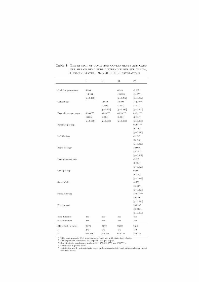
Table 1: The effect of coalition governments and cabi-net size on real public expenditures per capita,German States, 1975-2010, OLS estimations
I II III IV
Coalition government 5.399 6.149 -2.937
(13.163) (13.128) (14.977)
[p=0.706] [p=0.702] [p=0.892]
Cabinet size 10.639 10.709 15.210**
(7.950) (7.953) (7.371)
[p=0.400] [p=0.382] [p=0.200]
Expenditures per cap.t−1 0.900*** 0.893*** 0.893*** 0.699***
(0.035) (0.034) (0.034) (0.044)
[p=0.000] [p=0.000] [p=0.000] [p=0.000]
Revenues per cap. 0.165***
(0.036)
[p=0.016]
Left ideology -11.847
(25.148)
[p=0.836]
Right ideology 12.600
(19.157)
[p=0.558]
Unemployment rate -1.635
(5.364)
[p=0.820]
GDP per cap. 0.000
(0.005)
[p=0.978]
Share of old -4.751
(13.107)
[p=0.920]
Share of young 38.878***
(10.240)
[p=0.046]
Election year 25.318*
(13.936)
[p=0.000]
Year dummies Yes Yes Yes Yes
State dummies Yes Yes Yes Yes
AR(1)-test (p-value) 0.276 0.279 0.280 0.248
N 475 475 475 459
F 615.478 676.243 672.350 760.785
a This table presents OLS regressions without and with state fixed effects.b The dependent variable is real expenditures per capita.c Stars indicate significance levels at 10% (*), 5% (**) and 1%(***).d z-statistics in parentheses.e z-statistics and hypothesis tests based on heteroscedasticity and autocorrelation robust
standard errors.
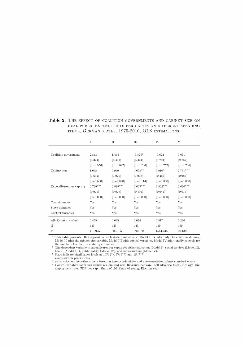
Table 2: The effect of coalition governments and cabinet size onreal public expenditures per capita on different spendingitems, German states, 1975-2010, OLS estimations
I II III IV V
Coalition government 2.843 1.444 -5.825* -0.622 0.671
(3.324) (4.453) (3.424) (1.204) (2.767)
[p=0.556] [p=0.822] [p=0.206] [p=0.752] [p=0.736]
Cabinet size 1.658 0.949 4.698** 0.910* 2.751***
(1.602) (1.975) (1.918) (0.469) (0.980)
[p=0.590] [p=0.820] [p=0.114] [p=0.308] [p=0.080]
Expenditures per cap.t−1 0.799*** 0.828*** 0.663*** 0.802*** 0.626***
(0.029) (0.029) (0.102) (0.042) (0.077)
[p=0.000] [p=0.000] [p=0.000] [p=0.000] [p=0.000]
Year dummies Yes Yes Yes Yes Yes
State dummies Yes Yes Yes Yes Yes
Control variables Yes Yes Yes Yes Yes
AR(1)-test (p-value) 0.455 0.695 0.024 0.817 0.296
N 443 443 443 459 459
F 419.925 803.195 392.188 1514.246 60.132
a This table presents OLS regressions with state fixed effects: Model I includes only the coalition dummy,Model II adds the cabinet size variable, Model III adds control variables, Model IV additionally controls forthe number of seats in the state parliament.
b The dependent variable is expenditures per capita for either education (Model I), social services (Model II),health (Model III), public safety (Model IV), and infrastructure (Model V).
b Stars indicate significance levels at 10% (*), 5% (**) and 1%(***).c z-statistics in parentheses.d z-statistics and hypothesis tests based on heteroscedasticity and autocorrelation robust standard errors.e Control variables for which results are omitted are: Revenues per cap., Left ideology, Right ideology, Un-
employment rate, GDP per cap., Share of old, Share of young, Election year.

Table 3: The effect of coalition governments and cabinetsize on real public expenditures per capita, Germanstates, 1975-2010, TSLS estimations
I II III IV
Coalition government -1.445 2.333 48.813 40.761
(-0.038) (0.061) (1.175) (0.978)
Cabinet size 10.666 14.233** 11.706*
(1.326) (1.965) (1.735)
Expenditures per cap.t−1 0.900*** 0.893*** 0.710*** 0.708***
(25.754) (26.524) (15.518) (16.544)
Parliament size 0.986*
(1.748)
Year dummies Yes Yes Yes Yes
State dummies Yes Yes Yes Yes
Control variables No No Yes Yes
AR(1)-test (p-value) 0.273 0.278 0.430 0.311
N 475 475 459 458
F 621.657 683.458 752.855 748.457
Kleibergen-Paap Wald F-Statistic 64.482 63.887 49.537 51.623
a This table presents TSLS regressions: Model I includes only the coalition dummy, Model IIadds the cabinet size variable, Model III adds control variables, Model IV additionally controlsfor the number of seats in the state parliament.
b The dependent variable is real expenditures per capita.b Stars indicate significance levels at 10% (*), 5% (**) and 1%(***).c z-statistics in parentheses.d z-statistics and hypothesis tests based on heteroscedasticity and autocorrelation robust standard
errors.e The Cragg-Donald Wald F-Statistic is used to test for weak instruments.f Control variables for which results are omitted are: Revenues per cap., Left ideology, Right
ideology, Unemployment rate, GDP per cap., Share of old, Share of young, Election year.
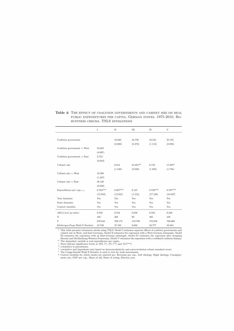
Table 4: The effect of coalition governments and cabinet size on realpublic expenditures per capita, German states, 1975-2010, Ro-bustness checks, TSLS estimations
I II III IV V
Coalition government 44.660 24.750 43.244 35.195
(0.889) (0.373) (1.113) (0.994)
Coalition government × West 54.823
(0.997)
Coalition government × East 2.753
(0.044)
Cabinet size 9.614 55.655** 9.159 11.807*
(1.540) (2.038) (1.293) (1.756)
Cabinet size × West 10.206
(1.497)
Cabinet size × East 20.126
(0.829)
Expenditures per cap.t−1 0.704*** 0.687*** 0.127 0.730*** 0.707***
(15.952) (12.561) (1.412) (17.130) (16.637)
Year dummies Yes Yes Yes Yes Yes
State dummies Yes Yes Yes Yes Yes
Control variables Yes Yes Yes Yes Yes
AR(1)-test (p-value) 0.502 0.534 0.630 0.183 0.238
N 458 368 90 405 458
F 670.643 708.172 119.790 710.032 736.960
Kleibergen-Paap Wald F-Statistic 18.739 37.450 9.692 52.777 56.564
a This table presents robustness checks using TSLS: Model I estimates separate effects of coalition governments andcabinet size in West- and East Germany, Model II estimates the regression with a West-German subsample, ModelIII estimates the regression with an East-German subsample, Model IV estimates the regression after droppingBavaria and Mecklenburg-Western Pomerania, Model V estimates the regression with a redefined coalition dummy.
b The dependent variable is real expenditures per capita.c Stars indicate significance levels at 10% (*), 5% (**) and 1%(***).d z-statistics in parentheses.e z-statistics and hypothesis tests based on heteroscedasticity and autocorrelation robust standard errors.f The Cragg-Donald Wald F-Statistic is used to test for weak instruments.g Control variables for which results are omitted are: Revenues per cap., Left ideology, Right ideology, Unemploy-
ment rate, GDP per cap., Share of old, Share of young, Election year.

(5169.318,6938.908](4901.404,5169.318](4172.498,4901.404](4050.028,4172.498][3852.593,4050.028]
Figure 1: Map of the 16 German States with average real expenditures percapita during the 1975-2010 period
3000
4000
5000
Real expenditure
s p
er
captia
1975 1980 1985 1990 1995 2000 2005 2010Year
Mean West−German States Mean East−German States
Figure 2: Development of (unweighted) average state expenditures percapita during the 1975-2010 period

01
23
45
6P
art
ies in p
arlia
ment
1975 1980 1985 1990 1995 2000 2005 2010Year
Mean Median
(a) Number of parties in parliament inWest-Germany
01
23
45
6P
art
ies in p
arlia
ment
1990 1995 2000 2005 2010Year
Mean Median
(b) Number of parties in parliament inEast-Germany
Figure 3: Development of the number of parties in West- and East-Germanstate parliaments
3.50
4.15
4.30
3.60
4.00
4.31
3.06
3.42
3.33
3.78
3.50
3.83
4.39
4.11
4.22
3.11
0 1 2 3 4 5Average number of parties %
East−Germany
West−Germany
TH
ST
SN
MV
BB
SH
SAAR
RP
NRW
NDS
HH
HE
HB
BW
BER
BAY
Figure 4: Average number of parties in the German state parliaments Def-inition of the state codes: BAY (Bavaria), BB (Brandenburg), BER (Berlin), BW (Baden-Wuerttemberg) HB (Bremen), HE (Hesse), HH (Hamburg), MV (Mecklenburg-Western Pomera-nia), NDS (Lower-Saxony), NRW (North Rhine-Westphalia), RP (Rhineland-Palatinate), SAAR(Saarland) SH (Schleswig-Holstein), SN (Saxony), ST (Saxony-Anhalt), TH (Thuringia)

0.1
.2.3
.4.5
Rela
tive fre
quency
CD
U−
FD
P
CD
U−
SP
D
SP
D−
FD
P
SP
D−
GR
EE
N
SP
D−
PD
S
CD
U
SP
D
SP
D−
GR
EE
N−
FD
P
CD
U−
GR
EE
N
CD
U−
GR
EE
N−
FD
P
Coalition
(a) Coalitions and single-party gov-ernments in West-Germany
0.1
.2.3
.4.5
Rela
tive fre
quency
CD
U−
FD
P
CD
U−
SP
D
SP
D−
FD
P
SP
D−
GR
EE
N
SP
D−
PD
S
CD
U
SP
D
SP
D−
GR
EE
N−
FD
P
CD
U−
GR
EE
N
CD
U−
GR
EE
N−
FD
P
Coalition
(b) Coalitions and single-party gov-ernments in East-Germany
Figure 5: Frequency of different types of government in West- and East-Germany
01
23
45
67
89
10
Num
ber
of coalit
ion g
overn
ments
1975 1980 1985 1990 1995 2000 2005 2010Year
(a) Number of coalition governmentsin West-Germany
01
23
45
67
89
10
Num
ber
of coalit
ion g
overn
ments
1990 1995 2000 2005 2010Year
(b) Number of coalition governmentsin East-Germany
Figure 6: Over-time developments of the number of coalition governmentsin West- and East-Germany

0.50
0.80
0.30
1.00
0.75
0.42
0.25
0.53
0.56
0.50
0.42
0.75
0.53
0.53
0.94
0.06
0 .2 .4 .6 .8 1Coalition governments in %
East−Germany
West−Germany
TH
ST
SN
MV
BB
SH
SAAR
RP
NRW
NDS
HH
HE
HB
BW
BER
BAY
Figure 7: Frequency of coalition governments in German States Definition ofthe state codes: BAY (Bavaria), BB (Brandenburg), BER (Berlin), BW (Baden-Wuerttemberg)HB (Bremen), HE (Hesse), HH (Hamburg), MV (Mecklenburg-Western Pomerania), NDS (Lower-Saxony), NRW (North Rhine-Westphalia), RP (Rhineland-Palatinate), SAAR (Saarland) SH(Schleswig-Holstein), SN (Saxony), ST (Saxony-Anhalt), TH (Thuringia)
89
10
11
12
13
Avera
ge c
abin
et siz
e
1975 1980 1985 1990 1995 2000 2005 2010Year
(a) Average cabinet size in West-Germany
89
10
11
12
13
Avera
ge c
abin
et siz
e
1990 1995 2000 2005 2010Year
(b) Average cabinet size in East-Germany
Figure 8: Development of the average cabinet size in West- and East-Germany

10.20
9.55
9.60
9.40
10.45
9.33
8.28
9.14
11.53
10.53
11.78
9.69
12.06
13.36
11.97
10.50
0 5 10 15Average cabinet size
East−Germany
West−Germany
TH
ST
SN
MV
BB
SH
SAAR
RP
NRW
NDS
HH
HE
HB
BW
BER
BAY
Figure 9: Average cabinet size in German States Definition of the state codes:BAY (Bavaria), BB (Brandenburg), BER (Berlin), BW (Baden-Wuerttemberg) HB (Bremen),HE (Hesse), HH (Hamburg), MV (Mecklenburg-Western Pomerania), NDS (Lower-Saxony),NRW (North Rhine-Westphalia), RP (Rhineland-Palatinate), SAAR (Saarland) SH (Schleswig-Holstein), SN (Saxony), ST (Saxony-Anhalt), TH (Thuringia)
4422.05
5012.55
01,0
00
2,0
00
3,0
00
4,0
00
5,0
00
Real expenditure
s p
er
capita
Single−party governments Coalition governments
(a) Coalition governments
3387.94
4419.21
4036.67
4610.634420.3
4776.224912.83
5757
4994.53
4471.71
7472.72
4514.41
02,0
00
4,0
00
6,0
00
8,0
00
Real expenditure
s p
er
capita
5 7 8 9 10 11 12 13 14 15 16 17
(b) Cabinet size
Figure 10: Coalition governments, cabinet size, and average public expen-ditures in the German States, 1975-2010

Appendix
A.1 Details on the coding of the cabinet size variable
Using the data provided by Schnapp (2006) to determine the number of cabinet minis-
ters involves some difficult choices. The most important issues are the following. First,
certain “Staatsekretare” (State Secretaries) have the same status as cabinet ministers in
some states (usually a Staatssekretar is a deputy of a minister and subordinate to him).
In particular, they can participate and vote in cabinet meetings. Second, some cabinets
have a minister who is responsible for “federal affairs”, whereas in other cabinets this
task is assumed by either the state prime minister or by cabinet ministers whose prime
responsibility is a different policy area. Third, each state has a “Staatskanzlei” (or alter-
natively a “Staatsministerium”) which is either led by a minister or a Staatssekretar. The
Staatskanzlei is different from the other ministries as it is essentially the office of the state
prime minister and coordinates policies among all other ministries. Fourth, sometimes one
minister leads two separate ministries.
I made the following decisions regarding the problematic cases described above. First,
I do not count Staatssekretare as members of the cabinet, except certain cases where the
Staatskanzlei is led by a Staatssekretar (see below) or where my data source explicitly
indicated that they were government members with seat and vote in the cabinet. Second,
I count the ministry for federal affairs as a separate ministry if it is led by a minister
who has no other cabinet post. (i. e. if it is led by a minister who has another cabinet
post – i. e. the state prime minister or some other cabinet minister– I do not count it
as a separate ministry.) Third, I do not count the Staatskanzlei as a separate ministry
except if the head of the Staatskanzlei (irrespective of whether he is formally a minister or
a Staatssekretar) is responsible for some additional tasks (for example, the Staatssekretar
in the cabinet formed in Baden-Wuerrtemberg from 2001 to 2006 was also responsible for
42

“European issues”, consequently I count the Staatskanzlei as a separate ministry in this
cabinet). Fourth, if one minister heads two separate ministers, I increase the cabinet size
by two.
There were some additional but relatively minor decisions I had to make, for example
regarding a reshuffling of the cabinet within an legislative period (I ascribe any changes in-
between election years to the year in which the reshuffling took place irrespective of whether
it happened in the first or second half) or how to treat an arrangement where a member of
the cabinet is a Staatssekretar but is called a minister (a so called “Staatssekretar mit der
Amtsbezeichnung Minister” – I count this Staatssekretar / minister as a proper member
of the cabinet).
A.2 Coalitions involving non-mainstream parties
Apart from the five mainstream parties, the party system consists of a multitude of fringe
parties. Most notably, there are several extreme right-wing parties which manage to enter
state parliaments from time to time (by obtaining more than five percent of the votes).20
The five mainstream parties, however, have always shunned them: extreme right-wing
parties were never part of any coalition government. Usually these extreme right-wing
parties only last one or two legislative period in parliament because they fail to receive
more than five percent of the votes in subsequent elections. Apart from the extreme right-
wing parties, there are a number of regionally based “protest” parties, i. e. parties which try
to offer an alternative to the established parties. The most notable was the so called Schill
Party (named after the founder of the party, the official name was Partei Rechtsstaatlicher
Offensive). This main focus of this party were law and order issues. After entering the state
parliament in Hamburg in the election of 2001, the Schill Party even formed a three-party
20Most notably the National Democratic Party of Germany (NPD), the Democratic Peoples’ Union(DVU), and the (German) Republicans (REP).
43

coalition government with the CDU and the FDP, with the CDU as the senior partner.
However, this government soon fall apart amids a scandal. Subsequently, the Schill Party
became irrelevant. In the following, I treat the CDU-FDP-Schill Party government during
the 2001-2004 period in Hamburg as a CDU-FDP government and thus as a right-wing
government.
Another important protest party was the STATT Party. This party entered the state
parliament of Hamburg in 1993. Subsequently, it concluded a “coalition-like” agreement
with the SPD by which the SPD received the support of the STATT Party. In exchange the
SPD agreed to appoint a number of ministers without party affiliations but chosen by the
STATT Party. While the STATT party thus played an important role for the government
of Hamburg during the 1993-1997 period, I nonetheless code this period as a sole SPD
government since no official members of the STATT Party were represented in the cabinet.
A.3 Uberhangmadate and Ausgleichsmandate
The Uberhangmadate and Ausgleichsmandate emerge in some states because of the at-
tempt of the electoral laws in these states to combine elements of both proportional and
plurality rule by means of the so called personalized proportional electoral system. In a
common variant of this electoral system, voters can cast two votes. With their first vote
(Erststimme), they vote for a candidate within their voting district. With their second
vote (Zweitstimme), they vote for a state party list. Seats in the state parliament are
alloted to the parties in general according their shares in the Zweitstimme. The share of
the Zweitstimme therefore basically defines the number of seats that should accrue to a
party. In the allocation of seats, candidates who are directly elected in their districts are
given primacy over candidates who are only on the party list. That is, seats that belong
to a party according to its share of the Zweitstimme are first filled with candidates who
44

have won in their districts. Any remaining seats are filled with candidates that are on the
party list (and have not won in their districts).
It can happen that the number candidates from a party who win in their districts exceeds
the number of seats a state can claim according to its share of the Zweitstimme. Since it
is not possible to deny a candidate who has won in his district a seat in parliament, the
party gets a Uberhangmandat, which increases the size of the parliament. Since this party
has now more seats than it should get according to its Zweitstimme, the electoral laws in
some states require that the other parties get so called Ausgleichsmadate. The purpose of
the Ausgleichsmandate is to correct the imbalance in the distribution of seats introduced
by the Uberhangmandate. The Ausgleichsmandate, if they exist, increase the size of the
parliament further.
A.4 Alternative instruments
In Table A.1, I report a number of robustness tests with alternative instruments, partly
to check the robustness of the regressions with the number of parties in parliament instru-
ment and partly to have the ability to calculate over-identification tests. These additional
instruments are the actual vote share of the FDP and the Green Party. Clearly, the larger
the share of votes that these two parties get, the less likely it will be that a single-party
government is formed. However, it is possible that these variables should not be excluded
from the second stage regression because if these two parties are actually part of the
government, their vote share might have a direct effect on public expenditures (the condi-
tional independence assumption is more suspect for these instruments than for the parties
in parliament instrument).
Model I in Table A.1 reports the result of a regression that replicates Model IV in Table
3, but uses the vote share of the FDP and the Green Party as instruments. Since two
instruments are available for one endogenous variable, Hansen-J over-identification tests
45
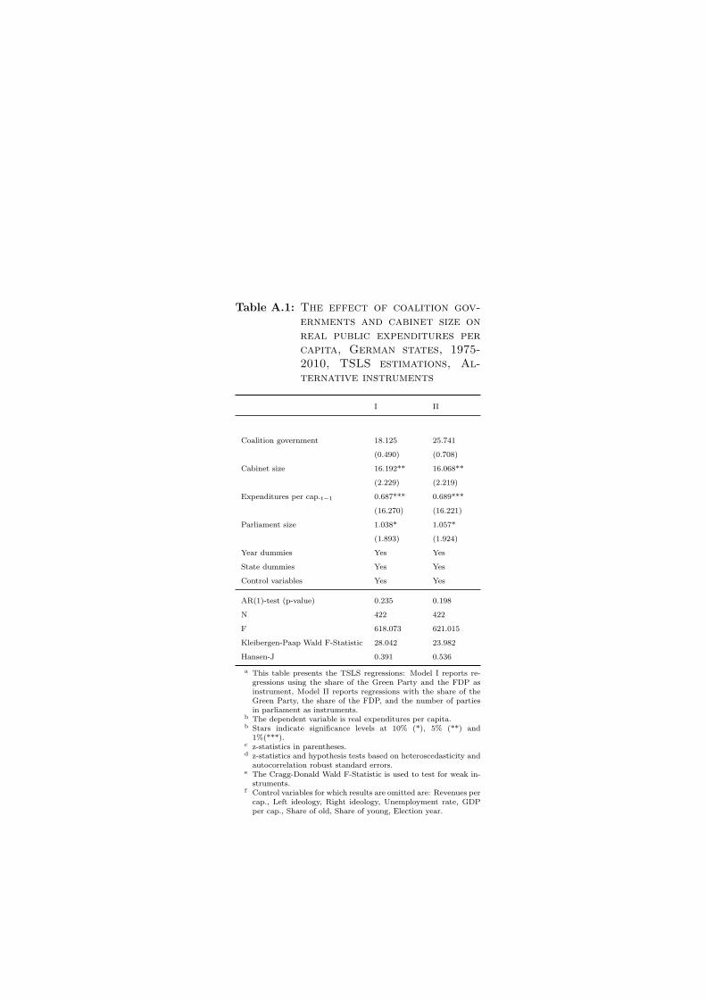
Table A.1: The effect of coalition gov-ernments and cabinet size onreal public expenditures percapita, German states, 1975-2010, TSLS estimations, Al-ternative instruments
I II
Coalition government 18.125 25.741
(0.490) (0.708)
Cabinet size 16.192** 16.068**
(2.229) (2.219)
Expenditures per cap.t−1 0.687*** 0.689***
(16.270) (16.221)
Parliament size 1.038* 1.057*
(1.893) (1.924)
Year dummies Yes Yes
State dummies Yes Yes
Control variables Yes Yes
AR(1)-test (p-value) 0.235 0.198
N 422 422
F 618.073 621.015
Kleibergen-Paap Wald F-Statistic 28.042 23.982
Hansen-J 0.391 0.536
a This table presents the TSLS regressions: Model I reports re-gressions using the share of the Green Party and the FDP asinstrument, Model II reports regressions with the share of theGreen Party, the share of the FDP, and the number of partiesin parliament as instruments.
b The dependent variable is real expenditures per capita.b Stars indicate significance levels at 10% (*), 5% (**) and
1%(***).c z-statistics in parentheses.d z-statistics and hypothesis tests based on heteroscedasticity and
autocorrelation robust standard errors.e The Cragg-Donald Wald F-Statistic is used to test for weak in-
struments.f Control variables for which results are omitted are: Revenues per
cap., Left ideology, Right ideology, Unemployment rate, GDPper cap., Share of old, Share of young, Election year.

can be calculated. The test, reported at the bottom of the table, does not indicate that
the instruments are invalid. The results with respect to the coalition dummy and the
cabinet size variable are almost similar to those reported in the previous sections. These
two variables are also strong instruments as indicated by the weak identification tests.
Model II replicates Model I by additionally including in the instrument set the number
of parties in parliament. In this model, the Hansen-J over-identification test can be inter-
preted as a test for the validity of the “parties in parliament” instrument. The Hansen-J
test is insignificant. The results for the coalition size and cabinet size variables are similar
to those reported in the previous section. While the validity of the over-identification tests
relies on the validity of at least one of the instruments, there is a reasonable chance that at
least one of the instruments is valid. It is therefore reassuring that the over-identification
tests are not rejected.
A.5 Dynamic panel data estimators
One problematic feature of the estimates reported in Table 1 in the main text is the reliance
of the large-T properties of the dataset to deal with the Nickell-bias. An alternative is to
rely on dynamic panel data estimators that have been developed to address the problem
of biased estimates in samples with small T. In this section, I report the results from
estimating Model 1 with four different dynamic panel data estimators: the Bias Corrected
Least Square Dummy Variables estimator, th Difference-GMM estimator, the System-
GMM estimator, and the Anderson-Hsiao estimator.
One feature of the Difference and System-GMM estimators is that the number of instru-
ments increases rapidly with the number of time periods, resulting in the so called “large
instrument problem” and unreliable inference (Roodman, 2008b). Clearly, these estima-
tors are designed for large-N-small-T datasets. Indeed, Judson and Owen (1999) do not
recommend the Difference- and System-GMM estimators with large T datasets.
47

According to Judson and Owen (1999), the Anderson-Hsiao estimator performs better
than System-GMM and Difference-GMM in datasets with large T (albeit not as well as the
simple fixed effects estimator). In contrast to the GMM-estimators, the number of instru-
ments in the Anderson-Hsiao estimator is relatively small. This estimator also starts out
by differencing Model 1. As instrument for the first difference lagged dependent variable,
the variant of the Anderson-Hsiao estimator that I apply here uses the second lag of the
level. The problem with the Anderson-Hsiao estimator is that it can be very inefficient if
the second lag of the dependent variable is not strongly correlated with the first difference
of the lagged dependent variable.
Table A.2 reports the result of estimating Model 1 with the four dynamic panel data
estimators. Model I reports the Bias Corrected LSDV regressions, Model II the Difference-
GMM regressions. Model III the System-GMM regressions. Model IV reports the Anderson-
Hsiao regressions using the second lag of the dependent variable as instrument. In Models
II-IV, I continue to use the number of parties in the state parliament as instrument for
the coalition government dummy. In Model I, the coalition variable is not instrumented
as the Bias Corrected LSDV estimator has not yet been extend to account for endogenous
regressors.
The coefficient for the coalition dummy is insignificant and numerically close to 0 in the
Bias Corrected LSDV regressions. It is positive and significant in the GMM regressions.
The numerical value of the estimate is around 100 in the Difference-GMM model, it is
somewhat smaller in the System-GMM model with 71. However, note that the diagnostic
tests do not perform well in these models. In particular, the Hansen-J test has a value
of 1, which points to the existence of a large instruments problem, confirming that the
GMM models are unreliable in large panels. The Anderson-Hsiao regression, too, produces
a fairly large (122.55) but insignificant estimate for the coalition dummy. Note, however,
once more that the diagnostic tests indicate that these models are unreliable. In particular,
48

the weak-identification statistic is very low for this model. Further inspection of the first-
stage results suggests that the small value of the test statistic can be explained by the fact
that the second lag of the dependent variable is not significantly correlated with the first
difference (the number of parties in parliament continues to be significantly and positively
related to the likelihood that a coalition government will be formed).
Results for the cabinet size variable also do not differ significantly between the dynamic
panel data models and the baseline results. The estimated coefficients are in around 10
and significant in Model I where the Bias Corrected LSDV estimator is used.
Table A.2: The effect of coalition governments and cabi-net size on real public expenditures per capita,German states, 1975-2010, Dynamic panel datamodels
I II III IV
Coalition government -1.144 98.720** 71.243* 122.551
(-0.052) (2.046) (1.719) (0.877)
Cabinet size 12.469* 10.090 5.754 10.257
(1.790) (0.834) (0.803) (0.998)
Expenditures per cap.t−1 0.740*** 0.668*** 0.826*** 0.691*
(16.649) (13.593) (11.010) (1.838)
Year dummies Yes Yes Yes Yes
Control variables Yes Yes Yes Yes
AR(1)-test (p-value) 0.204 0.330
N 458 442 458 442
χ2 598.412 2382.288
F 16.226
Hansen-J 1.000 1.000
GMM AR(1)-test (p-value) 0.009 0.009
GMM AR(2)-test (p-value) 0.610 0.489
Instrument-No. . 79 79 2
Kleibergen-Paap Wald F-Statistic 2.533
a This table presents robustness checks using dynamic panel data estimators: Model I are BiasCorrected LSDV results, Model II are Difference-GMM results, Model III are System-GMMresults, Model IV are Anderson-Hsiao regressions with the second lag of the dependent variableas instrument for its first difference.
b The dependent variable is real expenditures per capita.c Stars indicate significance levels at 10% (*), 5% (**) and 1%(***).d z-statistics in parentheses.e z-statistics and hypothesis tests based on bootstrapped (Bias Corrected LSDV), one-step ro-
bust (Difference-GMM and System GMM regressions) or heteroscedasticity and autocorrelationrobust (Anderson-Hsiao regressions) standard errors.
f Control variables for which results are omitted are: Revenues per cap., Left ideology, Rightideology, Unemployment rate, GDP per cap., Share of old, Share of young, Election year.
49

A.6 First-stage regressions, data sources, and summary statistics
Table A.3: First-stage regression of coalition govern-ments on parties in parliament, Germanstates, 1975-2010
I II III IV
Parties in parliament 0.267*** 0.267*** 0.235*** 0.242***
(8.030) (7.993) (7.038) (7.185)
Share of FDP
Share of Green Party
Cabinet size -0.003 0.024 0.035*
(-0.160) (1.342) (1.836)
Expenditures per cap.t−1 0.000* 0.000 -0.000* -0.000*
(1.658) (1.642) (-1.742) (-1.811)
Parliament size -0.004**
(-2.016)
Year dummies Yes Yes Yes Yes
State dummies Yes Yes Yes Yes
Control variables No No Yes Yes
N 475 475 459 458
F 10.991 11.473 21.885 22.264
a This table presents the first-stage regressions for the regressions reported in Table 3.b The dependent variable is whether a state is ruled by a coalition government.c Stars indicate significance levels at 10% (*), 5% (**) and 1%(***).d z-statistics in parentheses.e z-statistics and hypothesis tests based on heteroscedasticity and autocorrelation and au-
tocorrelation robust standard errors.f Control variables for which results are omitted are: Revenues per cap., Left ideology,
Right ideology, Unemployment rate, GDP per cap., Share of old, Share of young, Electionyear.
50

Table A.4: Definition and source of variables
Label Description Source
Expenditures per cap. Real consolidated expenditures per capita (de-flated by federal CPI). Expenditures are consol-idated between states and their localities.
German Federal Statis-tical Office
Education expendi-tures per cap.
Real net consolidated expenditures per capita foreducation (deflated by federal CPI). Net expen-ditures are consolidated between states and theirlocalities and corrected for certain transfers fromother parts of the public sector.
German Federal Statis-tical Office
Social expenditures percap.
Real net consolidated expenditures per capita forsocial services (deflated by federal CPI). Net ex-penditures are consolidated between states andtheir localities and corrected for certain transfersfrom other parts of the public sector.
German Federal Statis-tical Office
Health expendituresper cap.
Real net consolidated expenditures per capita forsocial services (deflated by federal CPI). Net ex-penditures are consolidated between states andtheir localities and corrected for certain transfersfrom other parts of the public sector.
German Federal Statis-tical Office
Public safety expendi-tures per cap.
Real net consolidated expenditures per capita forpublic safety (deflated by federal CPI). Net expen-ditures are consolidated between states and theirlocalities and corrected for certain transfers fromother parts of the public sector.
German Federal Statis-tical Office
Infrastructure expendi-tures per cap.
Real net consolidated expenditures for traffic andcommunications (deflated by federal CPI). Net ex-penditures are consolidated between states andtheir localities and corrected for certain transfersfrom other parts of the public sector.
German Federal Statis-tical Office
Coalition government Dummy variable = 1 if government is formed by acoalition of parties.
Own construc-tion based onwww.tagesschau.de
Cabinet size Number of ministers in the cabinet. Own constructionbased on Schnapp(2006) and informationsupplied by stategovernments or stateparliaments.
Parties in parliament Number of parties in the state parliament. www.election.de
Revenues per cap. Real revenues per capita (deflated by federal CPI).Revenues are consolidated between states andtheir localities.
German Federal Statis-tical Office
Left ideology Dummy = 1 if government is formed by left-leaning parties (i. e. for SPD, SPD-Green Party,and SPD-PDS governments).
Own construc-tion based onwww.tagesschau.de
Right ideology Dummy = 1 if government is formed by right-leaning parties (i. e. for CDU and CDU-FDP gov-ernments).
Own construc-tion based onwww.tagesschau.de
Unemployment State unemployment rate. German FederalAgency of Employ-ment
GDP per cap. Real GDP per capita (deflated by federal CPI). German Federal andState Statistical Offices(Arbeitskreis VGR derLander)
Share of old Share of “old” (≥65 years) in state population. German Federal Statis-tical Office
Share of young Share of “young” (≤15 years) in state population. German Federal Statis-tical Office
Election year Dummy = 1 if state election year. Own construc-tion based onwww.bundeswahlleiter.de
Parliament size Number of seats in parliament. German Federal Statis-tical Office

Table A.5: Summary statistics
Variable Mean Std. Dev. Min. Max. N
Expenditures per cap. overall 4752.904 1032.661 3179.423 7746.345 475between 885.706 3870.982 6959.696 16within 458.898 3283.635 6225.218 29.688
Education expendi-tures per cap.
overall 1081.836 194.924 725.734 1658.934 467
between 150.579 901.850 1452.110 16within 120.721 810.796 1396.853 29.188
Social expenditures percap.
overall 730.943 289.638 269.108 1589.493 467
between 215.402 461.664 1275.407 16within 180.711 278.797 1161.214 29.188
Health expendituresper cap.
overall 271.524 164.954 115.182 919.224 467
between 86.581 172.406 495.608 16within 140.989 -55.694 811.156 29.188
Public safety expendi-tures per cap.
overall 360.223 109.633 178.895 653.015 475
between 95.391 255.702 608.618 16within 47.198 245.117 476.646 29.688
Infrastructure expendi-tures per cap.
overall 174.218 53.676 1.829 355.262 475
between 39.791 118.579 273.696 16within 38.985 18.792 378.046 29.688
Coalition government overall 0.528 0.500 0.000 1.000 475between 0.245 0.057 1.000 16within 0.442 -0.414 1.471 29.688
Cabinet size overall 10.575 1.857 5.000 17.000 475between 1.369 8.257 13.457 16within 1.224 6.403 14.632 29.688
Parties in parliament overall 3.762 0.888 2.000 7.000 475between 0.444 3.057 4.429 16within 0.768 1.962 6.334 29.688
Revenues per cap. overall 4323.279 832.469 2733.492 7458.146 459between 691.436 3575.866 5859.317 16within 489.938 2695.959 6395.827 28.688
Left ideology overall 0.341 0.475 0.000 1.000 475between 0.236 0.000 0.743 16within 0.415 -0.402 1.198 29.688
Right ideology overall 0.425 0.495 0.000 1.000 475between 0.307 0.000 1.000 16within 0.396 -0.460 1.314 29.688
Unemployment overall 10.714 4.786 2.100 22.100 475between 4.594 5.454 19.133 16within 2.667 1.745 19.345 29.688
GDP per cap. overall 24448.760 6996.149 13488.820 46840.990 475between 5598.929 18186.260 38879.420 16within 4439.226 11615.050 32410.330 29.688
Share of old overall 17.181 2.505 11.643 24.677 475between 1.190 15.494 20.100 16within 2.275 12.018 22.547 29.688
Share of young overall 16.100 2.473 10.772 23.631 475between 1.565 13.631 17.924 16within 2.001 12.441 22.469 29.688
Election year overall 0.234 0.424 0.000 1.000 475between 0.027 0.200 0.286 16within 0.423 -0.052 1.034 29.688
Parliament size overall 123.587 48.159 50.000 241.000 474between 45.855 50.886 214.600 16within 13.073 89.987 200.044 29.625

Bisher erschienene Diskussionspapiere
Nr. 165 Baskaran, Thushyanthan: Coalition governments, cabinets size, and the common pool problem: evidence from the German States, Juli 2013
Nr. 164 Baskaran, Thushyanthan: Taxation and democratization, Juli 2013
Nr. 163 Baskaran, Thushyanthan; Mariana Lopes da Fonseca: The economics and empirics of tax competition: a survey, Juli 2013
Nr. 162 Aytimur, Refik Emre: Importance of Status Quo when Lobbying a Coalition Government, Juni 2013
Nr. 161 Aytimur, Refik Emre: Extreme Parties and Political Rents, Juni 2013
Nr. 160 Strulik, Holger: Optimal Aging with Uncertain Death, Juni 2013
Nr. 159 Prettner, Klaus; Strulik, Holger: Trade and Productivity: The Family Connection Redux, Juni 2013
Nr. 158 Vogt, Nora; Bizer, Kilian: Lock-in effects in competitive bidding schemes for payments for ecosystem services, Juni 2013
Nr. 157 Baskaran, Thushyanthan: Identifying local tax mimicking: administrative borders and a policy reform, Juni 2013
Nr. 156 Herwartz, Helmut; Walle, Yabibal M.: State dependence in the finance-growth nexus: a functional coefficient approach, Juni 2013
Nr. 155 Krenz, Astrid: Cross-country heterogeneity and endogeneity bias in life satisfaction estimations-macro- and micro-level evidence for advanced, developing and transition countries, Mai 2013
Nr. 154: Krenz, Astrid: Services Sector’s Concentration: the European Union, Greece, and the New Economic Geography, Mai 2013
Nr. 153: Ahmed, Junaid; Martinez-Zarzoso, Inmaculada: Blessing or Curse: The Stabilizing Role of Remittances, Foreign Aid and FDI to Pakistan, Mai 2013
Nr: 152: Strulik, Holger; Werner, Katharina: 50 is the New 30 – Long-run Trends of Schooling and Retirement Explained by Human Aging, März 2013
Nr. 151: Dalgaard, Carl-Johan; Strulik,Holger: The History Augmented Solow Model, März 2013
Nr. 150: Strulik, Holger; Trimborn, Timo: The Dark Side of Fiscal Stimulus, Januar 2013
Nr. 149: Prettner, Klaus: Public education, technological change and economic prosperity, Januar 2013
Nr. 148: Lankau, Matthias; Bicskei, Marianna; Bizer, Kilian: Cooperation Preferences in the Provision of Public Goods: An Experimental Study on the Effects of Social Identity, Dezember 2012
Nr. 147: Krenz, Astrid: Modeling Services Sectors' Agglomeration within a New Economic Geography Model, Dezember 2012
Nr. 146: Krenz, Astrid: A Panel Co-integration Analysis of Industrial and Services Sectors' Agglomeration in the European Union, Dezember 2012
Nr. 145: Strulik, Holger: Knowledge and Growth in the Very Long Run, November 2012
Nr. 144: Baskaran, Thushyanthan: Ideology and fiscal policy: quasi-experimental evidence from the German States, Oktober 2012
Nr. 143: Ehlers, Tim; Schwager, Robert: Honest Grading, Grade Inflation and Reputation, Oktober 2012
Nr. 142: Gehringer, Agnieszka: Another look at the determinants of current account imbalances in the European Union: An empirical assessment, Oktober 2012

Nr. 141: Strulik, Holger; Werner, Katharina: Life Expectancy, Labor Supply, and Long-Run Growth: Reconciling Theory and Evidence, September 2012
Nr. 140: Strulik, Holger; Prettner, Klaus; Prskawetz, Alexia: The Past and Future of Knowledge-based Growth, September 2012
Nr. 139: Prettner, Klaus; Trimborn, Timo: Demographic change and R&D-based economic growth: reconciling theory and evidence, September 2012
Nr. 138: König, Jörg; Ohr, Renate: Homogeneous groups within a heterogeneous community -Evidence from an index measuring European economic integration, August 2012
Nr. 137: Schwager, Robert: Student Loans in a Tiebout Model of Higher Education, Juli 2012
Nr. 136: Martínez-Zarzoso, Inmaculada: Exporting and Productivity: Evidence for Egypt and Morocco, April 2012
Nr. 135: König, Jörg; Ohr, Renate: Messung ökonomischer Integration in der Europäischen Union –Entwicklung eines EU-Integrationsindexes -, April 2012
Nr. 134: Gehringer, Agnieszka: Financial liberalization, growth, productivity and capital accumulation: The case of European integration, März 2012
Nr. 133: Berner, Eike; Birg, Laura: Retailers and Consumers. The pass-through of import price changes, März 2012
Nr. 132: Gehringer, Angnieszka: Current accounts in Europe: implications of the external imbalances for the future of the common monetary policy, März 2012
Nr. 131: Ohr, Renate; Özalbayrak, Mehmet: The Euro – A „MUST“ for Small European States?, Januar 2012
Nr. 130: Zeddies, Götz: Der Euro als Triebfeder des deutschen Exports?, November 2011
Nr. 129: Geishecker, Ingo; Siedler, Thomas: Job Loss Fears and (Extreme) Party Identification: First Evidence from Panel Data, Oktober 2011
Nr. 128: König, Jörg; Ohr, Renate: Small but Beautiful? Economic Impacts of the Size of Nations in the European Union, August 2011
Nr. 127: Schüder, Stefan: Monetary Policy Trade-Offs in a Portfolio Model with Endogenous Asset Supply, Juni 2011
Nr. 126: Hiller, Sanne: The Export Promoting Effect of Emigration: Evidence from Denmark, Juni 2011
Nr. 125: Martínez-Zarzoso, Inmaculada; Voicu, Anca M.; Vidovic, Martina: CEECs Integration into Regional and Global Production Networks, Mai 2011
Nr. 124: Roth, Felix; Gros, Daniel; Nowak-Lehmann D., Felicitas: Has the Financial Crisis eroded Citizens’ Trust in the European Central Bank? Panel Data Evidence for the Euro Area, 1999-2011, Mai 2011, Revised Version März 2012
Nr. 123 Dreher, Axel; Vreeland, James Raymond : Buying Votes and International Organizations, Mai 2011
Nr. 122: Schürenberg-Frosch, Hannah: One Model fits all? Determinants of Transport Costs across Sectors and Country Groups, April 2011
Nr. 121: Verheyen, Florian: Bilateral Exports from Euro Zone Countries to the US - Does Exchange Rate Variability Play a Role?, April 2011
Nr. 120: Ehlers, Tim: University Graduation Dependent on Family’s Wealth, Ability and Social Status, April 2011
Nr. 119: Cho, Seo-Young; Dreher, Axel; Neumayer, Eric: The Spread of Anti-trafficking Policies – Evidence from a New Index, März 2011
Nr. 118: Cho, Seo-Young; Vadlamannati, Krishna Chaitanya: Compliance for Big Brothers: An Empirical Analysis on the Impact of the Anti-trafficking Protocol, Februar 2011

Nr. 117: Nunnenkamp, Peter; Öhler, Hannes: Donations to US based NGOs in International Development Cooperation: How (Un-)Informed Are Private Donors?, Februar 2011
Nr. 116: Geishecker, Ingo; Riedl, Maximilian: Ordered Response Models and Non-Random Personality Traits: Monte Carlo Simulations and a Practical Guide, Revised Version Februar 2012
Nr. 115: Dreher, Axel; Gassebner, Martin; Siemers, Lars-H. R.: Globalization, Economic Freedom and Human Rights, Oktober 2010
Nr. 114: Dreher, Axel; Mikosch, Heiner; Voigt, Stefan: Membership has its Privileges – The Effect of Membership in International Organizations on FDI, Oktober 2010
Nr. 113: Fuchs, Andreas; Klann, Nils-Hendrik: Paying a Visit: The Dalai Lama Effect on International Trade, Oktober 2010
Nr. 112: Freitag, Stephan: Choosing an Anchor Currency for the Pacific, Oktober 2010
Nr. 111: Nunnenkamp, Peter; Öhler, Hannes: Throwing Foreign Aid at HIV/AIDS in Developing Countries: Missing the Target?, August 2010
Nr. 110: Ohr, Renate; Zeddies, Götz: „Geschäftsmodell Deutschland“ und außenwirtschaftliche Ungleichgewichte in der EU, Juli 2010
Nr. 109: Nunnenkamp, Peter; Öhler, Hannes: Funding, Competition and the Efficiency of NGOs: An Empirical Analysis of Non-charitable Expenditure of US NGOs Engaged in Foreign Aid, Juli 2010
Nr. 108: Krenz, Astrid: La Distinction reloaded: Returns to Education, Family Background, Cultural and Social Capital in Germany, Juli 2010
Nr. 107: Krenz, Astrid: Services sectors' agglomeration and its interdependence with industrial agglomeration in the European Union, Juli 2010
Nr. 106: Krenz, Astrid; Rübel, Gerhard: Industrial Localization and Countries' Specialization in the European Union: An Empirical Investigation, Juli 2010
Nr. 105: Schinke, Jan Christian: Follow the Sun! How investments in solar power plants in Sicily can generate high returns of investments and help to prevent global warming, Juni 2010
Nr. 104: Dreher, Axel; Sturm, Jan-Egbert; Vreeland, James Raymon: Does membership on the Security Council influence IMF conditionality?, Juni 2010
Nr. 103: Öhler, Hannes; Nunnenkamp, Peter; Dreher, Axel: Does Conditionality Work? A Test for an Innovative US Aid Scheme, Juni 2010
Nr. 102: Gehringer, Agnieszka: Pecuniary Knowledge Externalities in a New Taxonomy: Knowledge Interactions in a Vertically Integrated System, Juni 2010
Nr. 101: Gehringer, Agnieszka: Pecuniary Knowledge Externalities across European Countries – are there leading Sectors?, Juni 2010
Nr. 100: Gehringer, Agnieszka: Pecuniary Knowledge Externalities and Innovation: Intersectoral Linkages and their Effects beyond Technological Spillovers, Juni 2010
Nr. 99: Dreher, Axel; Nunnenkamp, Peter; Öhler, Hannes: Why it pays for aid recipients to take note of the Millennium Challenge Corporation: Other donors do!, April 2010
Nr. 98: Baumgarten, Daniel; Geishecker, Ingo; Görg, Holger: Offshoring, tasks, and the skill-wage pattern, März 2010
Nr. 97: Dreher, Axel; Klasen, Stephan; Raymond, James; Werker, Eric: The costs of favoritism: Is politically-driven aid less effective?, März 2010
Nr. 96: Dreher, Axel; Nunnenkamp, Peter; Thiele, Rainer: Are ‘New’ Donors Different? Comparing the Allocation of Bilateral Aid between Non-DAC and DAC Donor Countries, März 2010
Nr. 95: Lurweg, Maren; Westermeier, Andreas: Jobs Gained and Lost through Trade – The Case of Germany, März 2010

Nr. 94: Bernauer, Thomas; Kalbhenn, Anna; Koubi, Vally; Ruoff, Gabi: On Commitment Levels and Compliance Mechanisms – Determinants of Participation in Global Environmental Agreements, Januar 2010
Nr. 93: Cho, Seo-Young: International Human Rights Treaty to Change Social Patterns – The Convention on the Elimination of All Forms of Discrimination against Women, Januar 2010
Nr. 92: Dreher, Axel; Nunnenkamp, Peter; Thiel, Susann; Thiele, Rainer: Aid Allocation by German NGOs: Does the Degree of Public Refinancing Matter?, Januar 2010
Nr. 91: Bjørnskov, Christian; Dreher, Axel; Fischer, Justina A. V.; Schnellenbach, Jan: On the relation between income inequality and happiness: Do fairness perceptions matter?, Dezember 2009
Nr. 90: Geishecker, Ingo: Perceived Job Insecurity and Well-Being Revisited: Towards Conceptual Clarity, Dezember 2009
Nr. 89: Kühl, Michael: Excess Comovements between the Euro/US dollar and British pound/US dollar exchange rates, November 2009
Nr. 88: Mourmouras, Alex, Russel, Steven H.: Financial Crises, Capital Liquidation and the Demand for International Reserves, November 2009
Nr. 87: Goerke, Laszlo, Pannenberg, Markus: An Analysis of Dismissal Legislation: Determinants of Severance Pay in West Germany, November 2009
Nr. 86: Marchesi, Silvia, Sabani, Laura, Dreher, Axel: Read my lips: the role of information transmission in multilateral reform design, Juni 2009
Nr. 85: Heinig, Hans Michael: Sind Referenden eine Antwort auf das Demokratiedilemma der EU?, Juni 2009
Nr. 84: El-Shagi, Makram: The Impact of Fixed Exchange Rates on Fiscal Discipline, Juni 2009
Nr. 83: Schneider, Friedrich: Is a Federal European Constitution for an Enlarged European Union Necessary? Some Preliminary Suggestions using Public Choice Analysis, Mai 2009
Nr. 82: Vaubel, Roland: Nie sollst Du mich befragen? Weshalb Referenden in bestimmten Politikbereichen – auch in der Europapolitik – möglich sein sollten, Mai 2009
Nr. 81: Williamson, Jeffrey G.: History without Evidence: Latin American Inequality since 1491, Mai 2009
Nr. 80: Erdogan, Burcu: How does the European Integration affect the European Stock Markets?, April 2009
Nr. 79: Oelgemöller, Jens; Westermeier, Andreas: RCAs within Western Europe, März 2009
Nr. 78: Blonski, Matthias; Lilienfeld-Toal, Ulf von: Excess Returns and the Distinguished Player Paradox, Oktober 2008
Nr. 77: Lechner, Susanne; Ohr, Renate: The Right of Withdrawal in the Treaty of Lisbon: A game theoretic reflection on different decision processes in the EU, Oktober 2008
Nr. 76: Kühl, Michael: Strong comovements of exchange rates: Theoretical and empirical cases when currencies become the same asset, Juli 2008
Nr. 75: Höhenberger, Nicole; Schmiedeberg, Claudia: Structural Convergence of European Countries, Juli 2008
Nr. 74: Nowak-Lehmann D., Felicitas; Vollmer, Sebastian; Martinez-Zarzoso, Inmaculada: Does Comparative Advantage Make Countries Competitive? A Comparison of China and Mexico, Juli 2008
Nr. 73: Fendel, Ralf; Lis, Eliza M.; Rülke, Jan-Christoph: Does the Financial Market Believe in the Phillips Curve? – Evidence from the G7 countries, Mai 2008
Nr. 72: Hafner, Kurt A.: Agglomeration Economies and Clustering – Evidence from German Firms, Mai 2008

Nr. 71: Pegels, Anna: Die Rolle des Humankapitals bei der Technologieübertragung in Entwicklungsländer, April 2008
Nr. 70: Grimm, Michael; Klasen, Stephan: Geography vs. Institutions at the Village Level, Februar 2008
Nr. 69: Van der Berg, Servaas: How effective are poor schools? Poverty and educational outcomes in South Africa, Januar 2008
Nr. 68: Kühl, Michael: Cointegration in the Foreign Exchange Market and Market Efficiency since the Introduction of the Euro: Evidence based on bivariate Cointegration Analyses, Oktober 2007
Nr. 67: Hess, Sebastian; Cramon-Taubadel, Stephan von: Assessing General and Partial Equilibrium Simulations of Doha Round Outcomes using Meta-Analysis, August 2007
Nr. 66: Eckel, Carsten: International Trade and Retailing: Diversity versus Accessibility and the Creation of “Retail Deserts”, August 2007
Nr. 65: Stoschek, Barbara: The Political Economy of Enviromental Regulations and Industry Compensation, Juni 2007
Nr. 64: Martinez-Zarzoso, Inmaculada; Nowak-Lehmann D., Felicitas; Vollmer, Sebastian: The Log of Gravity Revisited, Juni 2007
Nr. 63: Gundel, Sebastian: Declining Export Prices due to Increased Competition from NIC – Evidence from Germany and the CEEC, April 2007
Nr. 62: Wilckens, Sebastian: Should WTO Dispute Settlement Be Subsidized?, April 2007
Nr. 61: Schöller, Deborah: Service Offshoring: A Challenge for Employment? Evidence from Germany, April 2007
Nr. 60: Janeba, Eckhard: Exports, Unemployment and the Welfare State, März 2007
Nr. 59: Lambsdoff, Johann Graf; Nell, Mathias: Fighting Corruption with Asymmetric Penalties and Leniency, Februar 2007
Nr. 58: Köller, Mareike: Unterschiedliche Direktinvestitionen in Irland – Eine theoriegestützte Analyse, August 2006
Nr. 57: Entorf, Horst; Lauk, Martina: Peer Effects, Social Multipliers and Migrants at School: An International Comparison, März 2007 (revidierte Fassung von Juli 2006)
Nr. 56: Görlich, Dennis; Trebesch, Christoph: Mass Migration and Seasonality Evidence on Moldova’s Labour Exodus, Mai 2006
Nr. 55: Brandmeier, Michael: Reasons for Real Appreciation in Central Europe, Mai 2006
Nr. 54: Martínez-Zarzoso, Inmaculada; Nowak-Lehmann D., Felicitas: Is Distance a Good Proxy for Transport Costs? The Case of Competing Transport Modes, Mai 2006
Nr. 53: Ahrens, Joachim; Ohr, Renate; Zeddies, Götz: Enhanced Cooperation in an Enlarged EU, April 2006
Nr. 52: Stöwhase, Sven: Discrete Investment and Tax Competition when Firms shift Profits, April 2006
Nr. 51: Pelzer, Gesa: Darstellung der Beschäftigungseffekte von Exporten anhand einer Input-Output-Analyse, April 2006
Nr. 50: Elschner, Christina; Schwager, Robert: A Simulation Method to Measure the Tax Burden on Highly Skilled Manpower, März 2006
Nr. 49: Gaertner, Wulf; Xu, Yongsheng: A New Measure of the Standard of Living Based on Functionings, Oktober 2005
Nr. 48: Rincke, Johannes; Schwager, Robert: Skills, Social Mobility, and the Support for the Welfare State, September 2005

Nr. 47: Bose, Niloy; Neumann, Rebecca: Explaining the Trend and the Diversity in the Evolution of the Stock Market, Juli 2005
Nr. 46: Kleinert, Jörn; Toubal, Farid: Gravity for FDI, Juni 2005
Nr. 45: Eckel, Carsten: International Trade, Flexible Manufacturing and Outsourcing, Mai 2005
Nr. 44: Hafner, Kurt A.: International Patent Pattern and Technology Diffusion, Mai 2005
Nr. 43: Nowak-Lehmann D., Felicitas; Herzer, Dierk; Martínez-Zarzoso, Inmaculada; Vollmer, Sebastian: Turkey and the Ankara Treaty of 1963: What can Trade Integration Do for Turkish Exports, Mai 2005
Nr. 42: Südekum, Jens: Does the Home Market Effect Arise in a Three-Country Model?, April 2005
Nr. 41: Carlberg, Michael: International Monetary Policy Coordination, April 2005
Nr. 40: Herzog, Bodo: Why do bigger countries have more problems with the Stability and Growth Pact?, April 2005
Nr. 39: Marouani, Mohamed A.: The Impact of the Mulitfiber Agreement Phaseout on Unemployment in Tunisia: a Prospective Dynamic Analysis, Januar 2005
Nr. 38: Bauer, Philipp; Riphahn, Regina T.: Heterogeneity in the Intergenerational Transmission of Educational Attainment: Evidence from Switzerland on Natives and Second Generation Immigrants, Januar 2005
Nr. 37: Büttner, Thiess: The Incentive Effect of Fiscal Equalization Transfers on Tax Policy, Januar 2005
Nr. 36: Feuerstein, Switgard; Grimm, Oliver: On the Credibility of Currency Boards, Oktober 2004
Nr. 35: Michaelis, Jochen; Minich, Heike: Inflationsdifferenzen im Euroraum – eine Bestandsaufnahme, Oktober 2004
Nr. 34: Neary, J. Peter: Cross-Border Mergers as Instruments of Comparative Advantage, Juli 2004
Nr. 33: Bjorvatn, Kjetil; Cappelen, Alexander W.: Globalisation, inequality and redistribution, Juli 2004
Nr. 32: Stremmel, Dennis: Geistige Eigentumsrechte im Welthandel: Stellt das TRIPs-Abkommen ein Protektionsinstrument der Industrieländer dar?, Juli 2004
Nr. 31: Hafner, Kurt: Industrial Agglomeration and Economic Development, Juni 2004
Nr. 30: Martinez-Zarzoso, Inmaculada; Nowak-Lehmann D., Felicitas: MERCOSUR-European Union Trade: How Important is EU Trade Liberalisation for MERCOSUR’s Exports?, Juni 2004
Nr. 29: Birk, Angela; Michaelis, Jochen: Employment- and Growth Effects of Tax Reforms, Juni 2004
Nr. 28: Broll, Udo; Hansen, Sabine: Labour Demand and Exchange Rate Volatility, Juni 2004
Nr. 27: Bofinger, Peter; Mayer, Eric: Monetary and Fiscal Policy Interaction in the Euro Area with different assumptions on the Phillips curve, Juni 2004
Nr. 26: Torlak, Elvisa: Foreign Direct Investment, Technology Transfer and Productivity Growth in Transition Countries, Juni 2004
Nr. 25: Lorz, Oliver; Willmann, Gerald: On the Endogenous Allocation of Decision Powers in Federal Structures, Juni 2004
Nr. 24: Felbermayr, Gabriel J.: Specialization on a Technologically Stagnant Sector Need Not Be Bad for Growth, Juni 2004
Nr. 23: Carlberg, Michael: Monetary and Fiscal Policy Interactions in the Euro Area, Juni 2004
Nr. 22: Stähler, Frank: Market Entry and Foreign Direct Investment, Januar 2004
Nr. 21: Bester, Helmut; Konrad, Kai A.: Easy Targets and the Timing of Conflict, Dezember 2003

Nr. 20: Eckel, Carsten: Does globalization lead to specialization, November 2003
Nr. 19: Ohr, Renate; Schmidt, André: Der Stabilitäts- und Wachstumspakt im Zielkonflikt zwischen fiskalischer Flexibilität und Glaubwürdigkeit: Ein Reform-ansatz unter Berücksichtigung konstitutionen- und institutionenökonomischer Aspekte, August 2003
Nr. 18: Ruehmann, Peter: Der deutsche Arbeitsmarkt: Fehlentwicklungen, Ursachen und Reformansätze, August 2003
Nr. 17: Suedekum, Jens: Subsidizing Education in the Economic Periphery: Another Pitfall of Regional Policies?, Januar 2003
Nr. 16: Graf Lambsdorff, Johann; Schinke, Michael: Non-Benevolent Central Banks, Dezember 2002
Nr. 15: Ziltener, Patrick: Wirtschaftliche Effekte des EU-Binnenmarktprogramms, November 2002
Nr. 14: Haufler, Andreas; Wooton, Ian: Regional Tax Coordination and Foreign Direct Investment, November 2001
Nr. 13: Schmidt, André: Non-Competition Factors in the European Competition Policy: The Necessity of Institutional Reforms, August 2001
Nr. 12: Lewis, Mervyn K.: Risk Management in Public Private Partnerships, Juni 2001
Nr. 11: Haaland, Jan I.; Wooton, Ian: Multinational Firms: Easy Come, Easy Go?, Mai 2001
Nr. 10: Wilkens, Ingrid: Flexibilisierung der Arbeit in den Niederlanden: Die Entwicklung atypischer Beschäftigung unter Berücksichtigung der Frauenerwerbstätigkeit, Januar 2001
Nr. 9: Graf Lambsdorff, Johann: How Corruption in Government Affects Public Welfare – A Review of Theories, Januar 2001
Nr. 8: Angermüller, Niels-Olaf: Währungskrisenmodelle aus neuerer Sicht, Oktober 2000
Nr. 7: Nowak-Lehmann, Felicitas: Was there Endogenous Growth in Chile (1960-1998)? A Test of the AK model, Oktober 2000
Nr. 6: Lunn, John; Steen, Todd P.: The Heterogeneity of Self-Employment: The Example of Asians in the United States, Juli 2000
Nr. 5: Güßefeldt, Jörg; Streit, Clemens: Disparitäten regionalwirtschaftlicher Entwicklung in der EU, Mai 2000
Nr. 4: Haufler, Andreas: Corporate Taxation, Profit Shifting, and the Efficiency of Public Input Provision, 1999
Nr. 3: Rühmann, Peter: European Monetary Union and National Labour Markets, September 1999
Nr. 2: Jarchow, Hans-Joachim: Eine offene Volkswirtschaft unter Berücksichtigung des Aktienmarktes, 1999
Nr. 1: Padoa-Schioppa, Tommaso: Reflections on the Globalization and the Europeanization of the Economy, Juni 1999
Alle bisher erschienenen Diskussionspapiere zum Download finden Sie im Internet unter: http://www.uni-goettingen.de/de/60920.html.