1

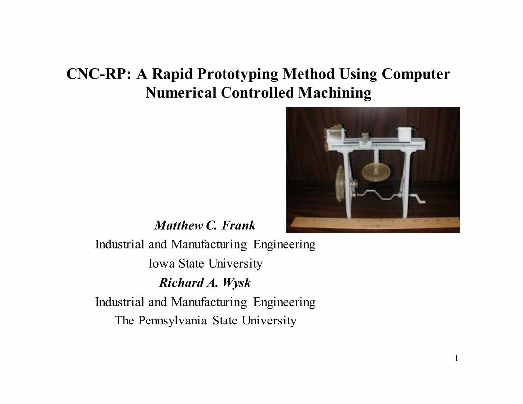
CNC-RP: A Rapid Prototyping Method Using Computer

Numerical Controlled Machining

Matthew C. Frank

Industrial and Manufacturing Engineering

Iowa State University

Richard A. Wysk

Industrial and Manufacturing Engineering

The Pennsylvania State University

2

Agenda

• What is RP?

• Limitations of RP

• Economics of RP

• New directions in RP

• Observations and conclusions

2

33

• Prototyping is critically important during product/process design

– Reduce time to market

– Early detection of errors

– Assist concurrent manufacturing engineering

• Prototypes are used to convey a products’:

– Form

– Fit

– Function

• Prototype building can be a time-consuming process requiring a highly skilled craftsperson

– Time spent testing prototypes is valuable

– Time spent constructing them is not…

• “Rapid Prototyping” (RP) methods have emerged

– (Solid Freeform Fabrication, Additive Manufacturing, Layered Manufacturing)

Need for model

accuracy increases

Introduction

4

Stereolithography (SLA)

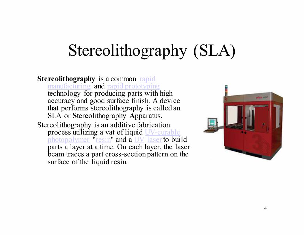
Stereolithography is a common rapid manufacturing and rapid prototypingtechnology for producing parts with high accuracy and good surface finish. A device that performs stereolithography is called an SLA or Stereolithography Apparatus.

Stereolithography is an additive fabrication process utilizing a vat of liquid UV-curablephotopolymer "resin" and a UV laser to build parts a layer at a time. On each layer, the laser beam traces a part cross-section pattern on the surface of the liquid resin.

5

Selective Laser Sintering (SLS)

SLS can produce parts from a relatively wide range of commercially available powder materials, including polymers (nylon, also glass-filled or with other fillers, and polystyrene), metals (steel, titanium, alloy mixtures, and composites) and green sand. The physical process can be full melting, partial melting, or liquid-phase sintering. And, depending on the material, up to 100% density can be achieved with material properties comparable to those from conventional manufacturing methods. In many cases large numbers of parts can be packed within the powder bed, allowing very high productivity.

6

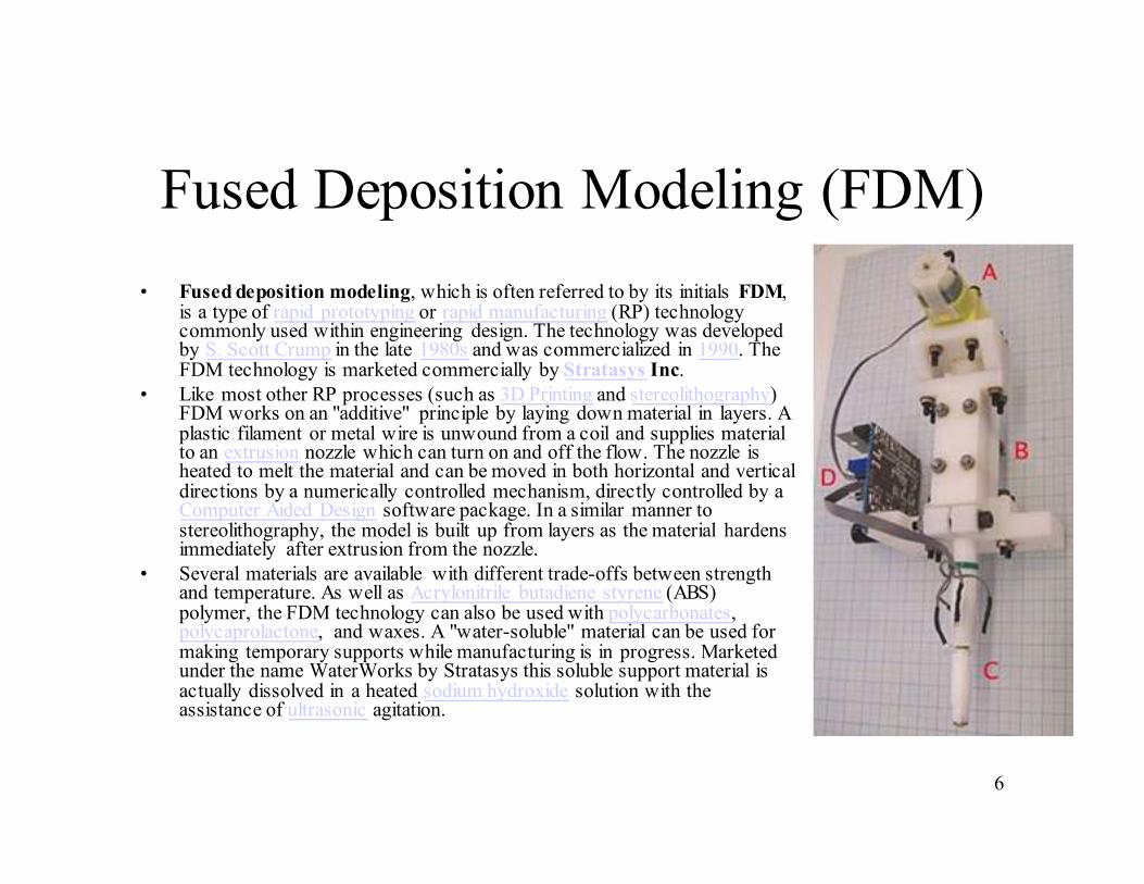
Fused Deposition Modeling (FDM)

• Fused deposition modeling, which is often referred to by its initials FDM, is a type of rapid prototyping or rapid manufacturing (RP) technology commonly used within engineering design. The technology was developed by S. Scott Crump in the late 1980s and was commercialized in 1990. The FDM technology is marketed commercially by Stratasys Inc.

• Like most other RP processes (such as 3D Printing and stereolithography) FDM works on an "additive" principle by laying down material in layers. A plastic filament or metal wire is unwound from a coil and supplies material to an extrusion nozzle which can turn on and off the flow. The nozzle is heated to melt the material and can be moved in both horizontal and vertical directions by a numerically controlled mechanism, directly controlled by a Computer Aided Design software package. In a similar manner to stereolithography, the model is built up from layers as the material hardens immediately after extrusion from the nozzle.

• Several materials are available with different trade-offs between strength and temperature. As well as Acrylonitrile butadiene styrene (ABS) polymer, the FDM technology can also be used with polycarbonates, polycaprolactone, and waxes. A "water-soluble" material can be used for making temporary supports while manufacturing is in progress. Marketed under the name WaterWorks by Stratasys this soluble support material is actually dissolved in a heated sodium hydroxide solution with the assistance of ultrasonic agitation.

7

Laminated Object Manufacturing

(LOM)

Laminated Object Manufacturing (LOM) is a rapid prototyping system developed by Helisys Inc. (Cubic Technologies is now the successor organization of Helisys) In it, layers of adhesive-coated paper, plastic, or metallaminates are successively glued together and cut to shape with a knife or laser cutter.

8

Electron Beam Melting (EBM)• Electron Beam Melting (EBM) is a type of rapid

prototyping for metal parts. It is often classified as a rapid manufacturing method. The technology manufactures parts by melting metal powder layer per layer with an electron beam in a high vacuum. Unlike some metal sintering techniques, the parts are fully solid, void-free, and extremely strong. Electron Beam Melting is also referred to as Electron Beam Machining.

• High speed electrons .5-.8 times the speed of light are bombarded on the surface of the work material generating enough heat to melt the surface of the part and cause the material to locally vaporize. EBM does require a vacuum, meaning that the workpiece is limited in size to the vacuum used. The surface finish on the part is much better than that of other manufacturing processes. EBM can be used on metals, non-metals, ceramics, and composites.

9

Types of RP Systems

Prototyping Technologies Base Materials

Selective laser sintering (SLS) Thermoplastics, metals powders

Fused Deposition Modeling (FDM) Thermoplastics, Eutectic metals.

Stereolithography (SLA) photopolymer

Laminated Object Manufacturing

(LOM)Paper

Electron Beam Melting (EBM) Titanium alloys

3D Printing (3DP) Various materials

10

Time and Cost to machine

11

Material cost

• In most cases this is independent of the

number of parts

11

12

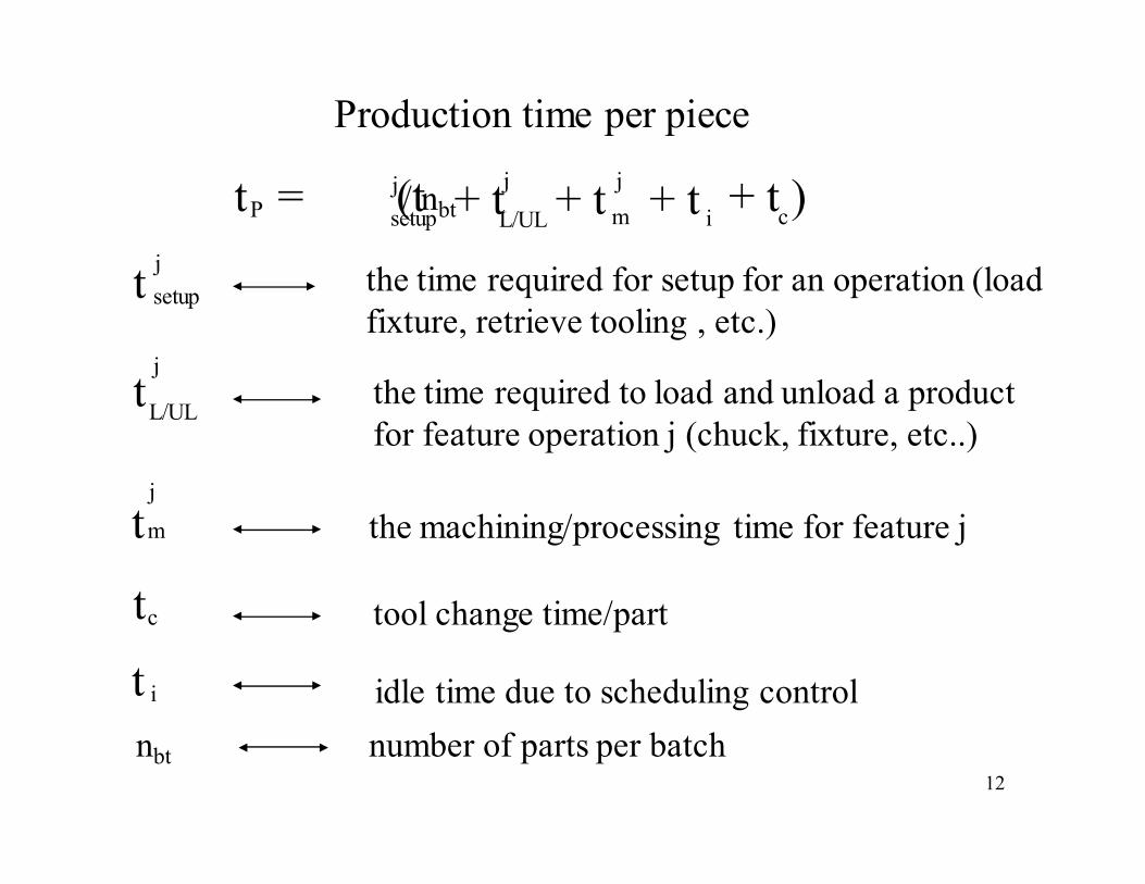
the time required for setup for an operation (load

fixture, retrieve tooling , etc.)

the time required to load and unload a product

for feature operation j (chuck, fixture, etc..)

the machining/processing time for feature j

tool change time/part

idle time due to scheduling control

L/UL

tj

j

setupt

tj

m

ct

t i

L/UL m c= (tj

setup+ t

j+ t

j+ t

i+ t )tP / nbt

Production time per piece

nbt number of parts per batch

13

• The product cost can be expressed

as:

Production cost per piece, Cp

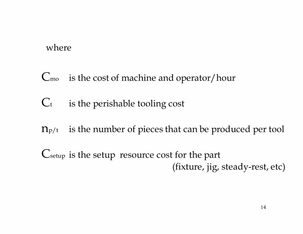
C CC Cp mo t p/t setup p/t= t p + /n + /n

14

Cmo is the cost of machine and operator/hour

Ct is the perishable tooling cost

np/t is the number of pieces that can be produced per tool

Csetup is the setup resource cost for the part

(fixture, jig, steady-rest, etc)

where

15

Problem Introduction

• Rapid Prototyping?

– Technology for producing accurate parts directly from CAD models in a few hours with little need for human intervention.

– Pham, et al, 1997

• Prototype?– A first full-scale and usually functional form of a new type or

design of a construction (as an airplane)– Webster’s, 1998

• Model?– A representation in relief or 3 dimensions in plaster, papier-mache,

wood, plastic, or other material of a surface or solid– Webster’s, 1986

physical models

How can we automatically create toolpath and fixture plans

for CNC?

16

Engineering cost

CE = Ced / nt + Cpc / nt + Cpd / nb

total parts total parts parts in a batch

16

17

Manufacturing cost

• One time costs– Process planning and design

– Fixture engineering and fabrication

• Set up cost (Cset)– Cost to set up a process

• Processing cost (Cpsc)– Cost of processing a part

• Production cost (Cpdc)– Cost of tooling and perishables

17

18

Manufacturing cost

CM = Cone / nt + Cset / nb + Cpsc + Cpdc // ntool

Total parts parts in a batch each part tool cost by parts/tool

18

19

So how can engineering costs be

reduced for CNC machining?

Machine cost Fixture cost Process planning cost

20

• CNC-RP Method: A part is machined on a 3-Axis mill with a

rotary indexer and tailstock using layer-based toolpaths from

numerous orientations about an axis of rotation.

TableOpposing

3-jaw chucks

Rotary indexer

Round stockEnd mill

Axis of rotation

TableOpposing

3-jaw chucks

Rotary indexer

Round stockEnd mill

Axis of rotation

21

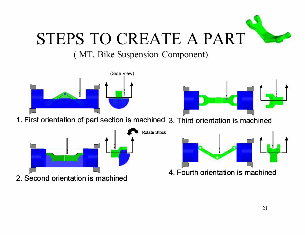
STEPS TO CREATE A PART ( MT. Bike Suspension Component)

1. First orientation of part section is machined

(Side View)

1. First orientation of part section is machined

(Side View) (Side View)

Rotate Stock

2. Second orientation is machined

Rotate StockRotate Stock

2. Second orientation is machined2. Second orientation is machined

3. Third orientation is machined3. Third orientation is machined

4. Fourth orientation is machined4. Fourth orientation is machined4. Fourth orientation is machined

22

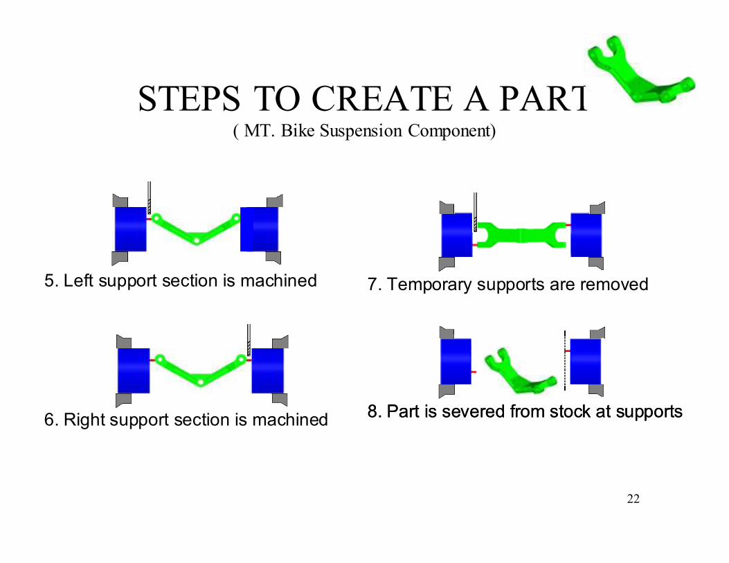
STEPS TO CREATE A PART ( MT. Bike Suspension Component)

5. Left support section is machined5. Left support section is machined

6. Right support section is machined6. Right support section is machined

7. Temporary supports are removed7. Temporary supports are removed

8. Part is severed from stock at supports8. Part is severed from stock at supports

23

Finished Steel Part

4”

Finished Steel Part

4”4”4”

Part fixtured with final 2 sacrificial supportsPart fixtured with final 2 sacrificial supports

Material: Steel

Layer depth: 0.001” (0.025mm)

Process/fixture planning time: Minutes

Processing time ~20 hours

24

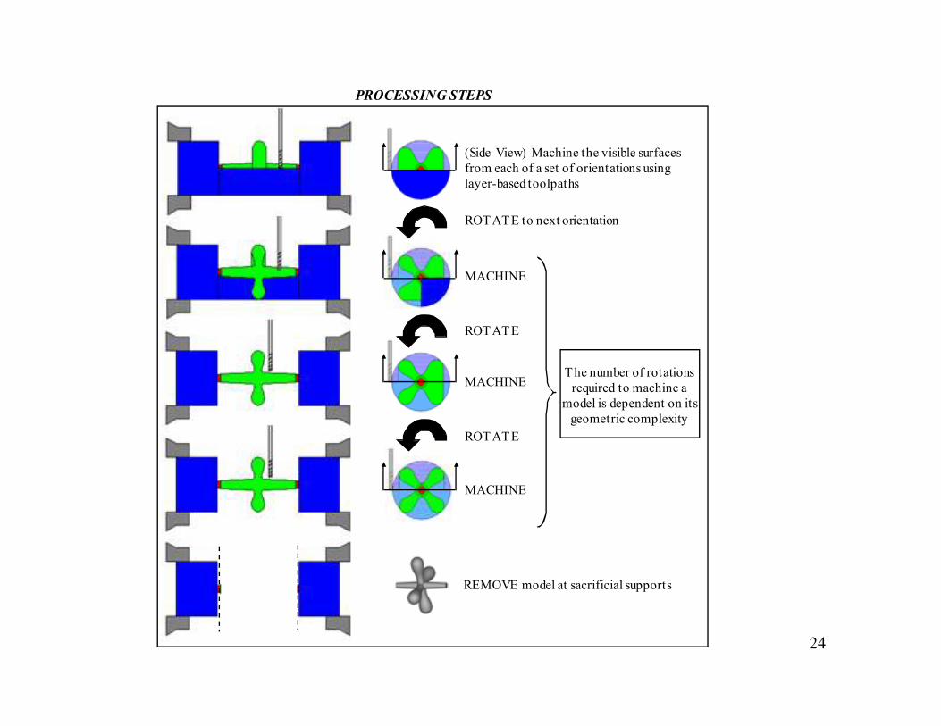
PROCESSING STEPS

(Side View) Machine the visible surfaces

from each of a set of orientations using

layer-based toolpaths

ROTATE to next orientation

MACHINE

ROTATE

MACHINE

ROTATE

MACHINE

REMOVE model at sacrificial supports

The number of rotations

required to machine a

model is dependent on its

geometric complexity

25

Methodology

• Creation of complex parts using a series of thin layers (slices) of 3-axis toolpaths generated at numerous orientations rotated about an axis of the part

• Toolpath planning based on “layering” methods used by other RP systems

• “Slice” represents visible cross-sectional area to be machined about (subtractive) rather than actual cross section to be deposited (additive)

• Slice thickness is the depth of cut for the 2½-D toolpaths

• Tool used is a flat end mill cutter with equal flute and shank diameter (or shank diameter < flute diameter)

• Stock material will be cylindrical, therefore toolpath z-zero location will be same for all orientations

26

Flat end mill cutter

Methodology (cont.)

“Staircase” effect

Region not visible from

current orientation

Set of visible slices from

current orientation

Toolpath planning using this approach is done with ease in current CAM

software (MasterCAM rough surface pocketing)

27

Methodology (cont.)

• Fixturing accomplished through temporary feature(s) (cylinders)

appended to the solid model prior to toolpath planning

• Cylinders attached to solid model along the axis of rotation

• Incrementally created during machining operation as the model is

rotated

• Model remains secured to stock material then removed (similar to

support structures in current RP methods)

28

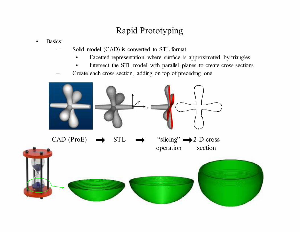
Rapid Prototyping• Basics:

– Solid model (CAD) is converted to STL format

• Facetted representation where surface is approximated by triangles

• Intersect the STL model with parallel planes to create cross sections

– Create each cross section, adding on top of preceding one

x

y

z

CAD (ProE) STL “slicing”

operation

2-D cross

section

29

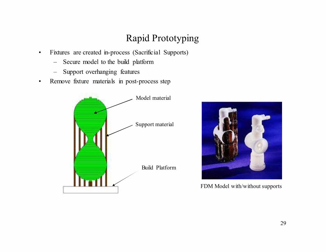
Rapid Prototyping

• Fixtures are created in-process (Sacrificial Supports)

– Secure model to the build platform

– Support overhanging features

• Remove fixture materials in post-process step

Model material

Support material

Build Platform

FDM Model with/without supports

30

RP versus CNC Machining

• RP processes are very flexible and very capable

• However:

– RP processes rely on specialized materials

– Limited accuracy in some cases

• CNC Machining is:

– Subtractive process

– Accurate

– Capable of using many common manufacturing materials

• CNC Machining is NOT:

– Automated

– Easily usable except by highly skilled technicians

• CNC machining cannot create all parts

• No hollow parts

• No severely undercut features

• The time consuming tasks of process and fixture planning are major factors which prohibit CNC machining from being used as a Rapid Prototyping Process

– Wang et al, 1999

Functional prototypes?

31

Previous Work

• Chen and Song, 1991

– Layer based machining for prototyping

– Machined layers using robotic arm/machine tool

– Layers laminated in a stack

• Merz, et al, 1994

– Shape Deposition Manufacturing

– Additive/Subtractive Process

• Walczyk and Hardt, 1998; Vouezelaud et al, 1992

– Rapid tooling

– Laminated machining for dies

• Lennings, 2000

– Deskproto software

– CNC machining planner

– Processes similar to a mill/turn operation

32

Motivation

• RP processes are almost completely automated “turnkey” operations

– User does not have to be skilled technician

– Process planning is simplified by layer-based approach

– Fixtures are created in process

• The approach to CNC-RP will have to relax many of the traditional constraints

– Efficient machining is not a major driver (Traditional feeds/speeds not used)

– Not feature-based (Not necessary to machine entire feature in one setup orientation)

– Surface finish not as critical (Allow staircase effect)

• Goal of this research is to develop a method for CNC rapid prototyping such that:

– Toolpath planning, sequencing, tool sizing is automated

– Fixture design is created in-process, flexible, and allows access to almost all

surfaces

– Setups/orientation automatically calculated, executed

– No collision problems

33

Methodology• Overview:

– Visible surfaces of the part are machined from each orientation about an axis of

rotation

– Long, small diameter flat end tool with equal flute and shank diameter used.

– Sacrificial supports (temporary features) added to the solid model and created in-

process

– Begin with round stock material, clamped between two opposing chucks

• Example:

x

y

z

x

y

z

Toolpath layers at 180º orientation

y

z

Toolpath layers at 0º orientation

y

z

34

Research Problems

• Setup/Orientation

– How many rotations (setup orientations) about the axis of rotation are required?

– Where are they?

• Toolpath planning

– For each orientation, how can we automatically generate toolpaths?

– What diameter and length tools should be used?

– In what order should the toolpaths be executed?

• Fixture planning

– How can we automatically generate sacrificial supports?

– What diameter and length should they be?

35

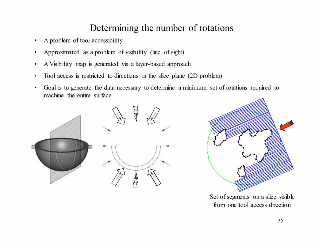
• A problem of tool accessibility

• Approximated as a problem of visibility (line of sight)

• A Visibility map is generated via a layer-based approach

• Tool access is restricted to directions in the slice plane (2D problem)

• Goal is to generate the data necessary to determine a minimum set of rotations required to

machine the entire surface

Set of segments on a slice visible

from one tool access direction

Determining the number of rotations

36

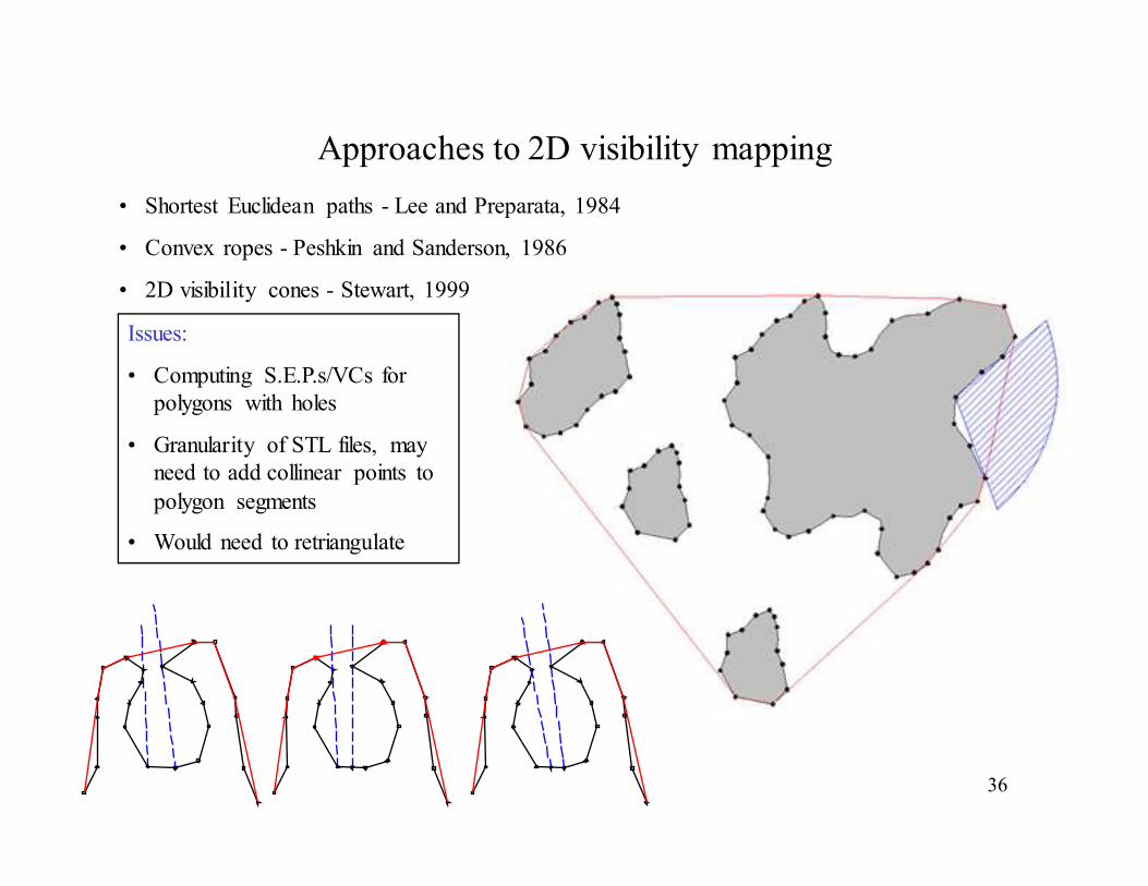
Approaches to 2D visibility mapping

• Shortest Euclidean paths - Lee and Preparata, 1984

• Convex ropes - Peshkin and Sanderson, 1986

• 2D visibility cones - Stewart, 1999

Issues:

• Computing S.E.P.s/VCs for

polygons with holes

• Granularity of STL files, may

need to add collinear points to

polygon segments

• Would need to retriangulate

37

(a) Visibility for the segment=

[Θa,Θb,]

(b) Visibility for the segment=

[Θa,Θb,], [Θc,Θd,]

Θa Θb

Θc

Θd Θa

Θb

• Visibility for each polygonal chain is determined by calculating

the polar angle range that each segment of the chain can be seen.

• Since there can be multiple chains on each slice, we must consider

the visibility blocked by all other chains.

Solution approach

38

Pi+1

P: ,

S :

Pi+1Pi-1

LCHP RCHP

LCHP RCHP

Pi

Pi

not

visible

• We have a polygon P and its convex hull S

• For any point Pi not on S, the visible range can be found by investigating points from the

adjacent CCW convex hull point to the adjacent CW convex hull point

• These points will be denoted the “left” and “right” convex hull points of Pi, LCHP(Pi) and

RCHP(Pi), respectively.

• It is only necessary to calculate the polar angles from Pi to the points in the set [LCHP,

RCHP], excluding Pi.

• The set is divided into, S1 and S2 where: ],[:2

],[:1

1

1

RCHPPS

PLCHPS

i

i

+

−

Step one: Visibility with respect to own chain

39

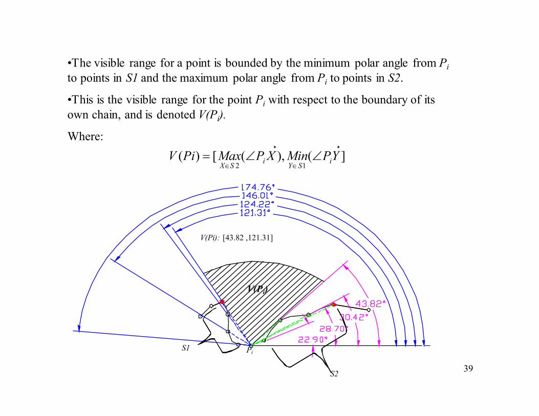
•The visible range for a point is bounded by the minimum polar angle from Pi

to points in S1 and the maximum polar angle from Pi to points in S2.

•This is the visible range for the point Pi with respect to the boundary of its

own chain, and is denoted V(Pi).

Where:

](),([)(12

YPMinXPMaxPiV iSY

iSX

∠∠=∈∈

V(Pi)

Pi

V(Pi): [43.82 ,121.31]

S1

S2

40

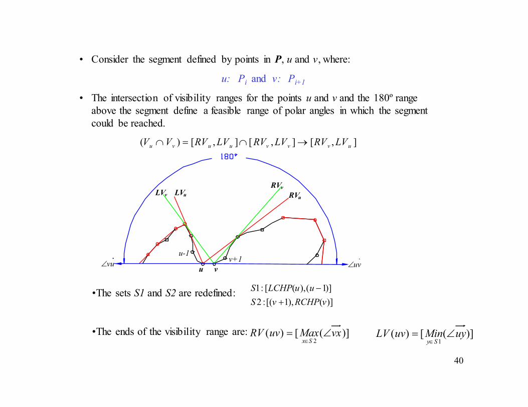
• Consider the segment defined by points in P, u and v, where:

u: Pi and v: Pi+1

• The intersection of visibility ranges for the points u and v and the 180º range

above the segment define a feasible range of polar angles in which the segment

could be reached.

],[],[],[)( uvvvuuvu LVRVLVRVLVRVVV →∩=∩

LVuLVv RVu

RVv

vu

v+1u-1

vu∠ uv∠

•The sets S1 and S2 are redefined:

•The ends of the visibility range are:

)](),1[(:2

)]1(),([:1

vRCHPvS

uuLCHPS

+

−

)]([)(2

vxMaxuvRVSx

∠=∈

)]([)(1

uyMinuvLVSy∠=

∈

41

Problem Surfaces

(a) RV is outside of the 180º range, (b) Both RV and LV are out of the 180º range, (c)

No visibility due to overlapping, (d) Visibility to the entire segment is not possible

since RV > LV.

(a) (b)

(c) (d)

u v

I1

I2

u v

I1 I2

u v

I1

I2 u vI1

I2

LV

RV

RV

LVRV

LV

RV LV

42

Step two: Visibility blocked by all other chains on the slice

• V( )j* is the visibility with respect to the chain j on which resides,

denoted j*.

• For all obstacle chains , the polar range blocked by the chain is

denoted VB( )j.

• The set of visible ranges for the segment is defined:

• Visibility blocked to the segment is the union of the visibility blocked by

chain j to point u and the visibility blocked by chain j to point v, intersected

with the 180º range above segment

• The set of angles blocked to the segment where:

• The set of angles blocked to points u and v where:

uv uv

( )*\ jJj ∈

uv

∑−=jj

uvVBuvVuvVIS )()()(*

uv

uv

]},[]])([])({[[)( vuuvvVBuVBuvVBjjj

∠∠∩∪=

],[)( uuj LBRBuVB = ],[)(vvj

LBRBvVB =

43

RBu

LBu RBv

LBv

u v

• Considering the condition that

blocked visibility is only for blockage

in the 180º range above the segment,

it can easily be seen that the set:

],[],[],[)( vuvvuuvu LBRBLBRBLBRBVBVB →∪=∪

• RBu is simply the minimum polar

angle from u to all points on the

blocker chain

• LBv is the maximum polar angle from

v to all points on Pj, where Pj is the

set of points for the blocker chain.

)]([ uxMinRBjPx

u ∠=∈

)]([ vyMaxLBjPy

v ∠=∈

44

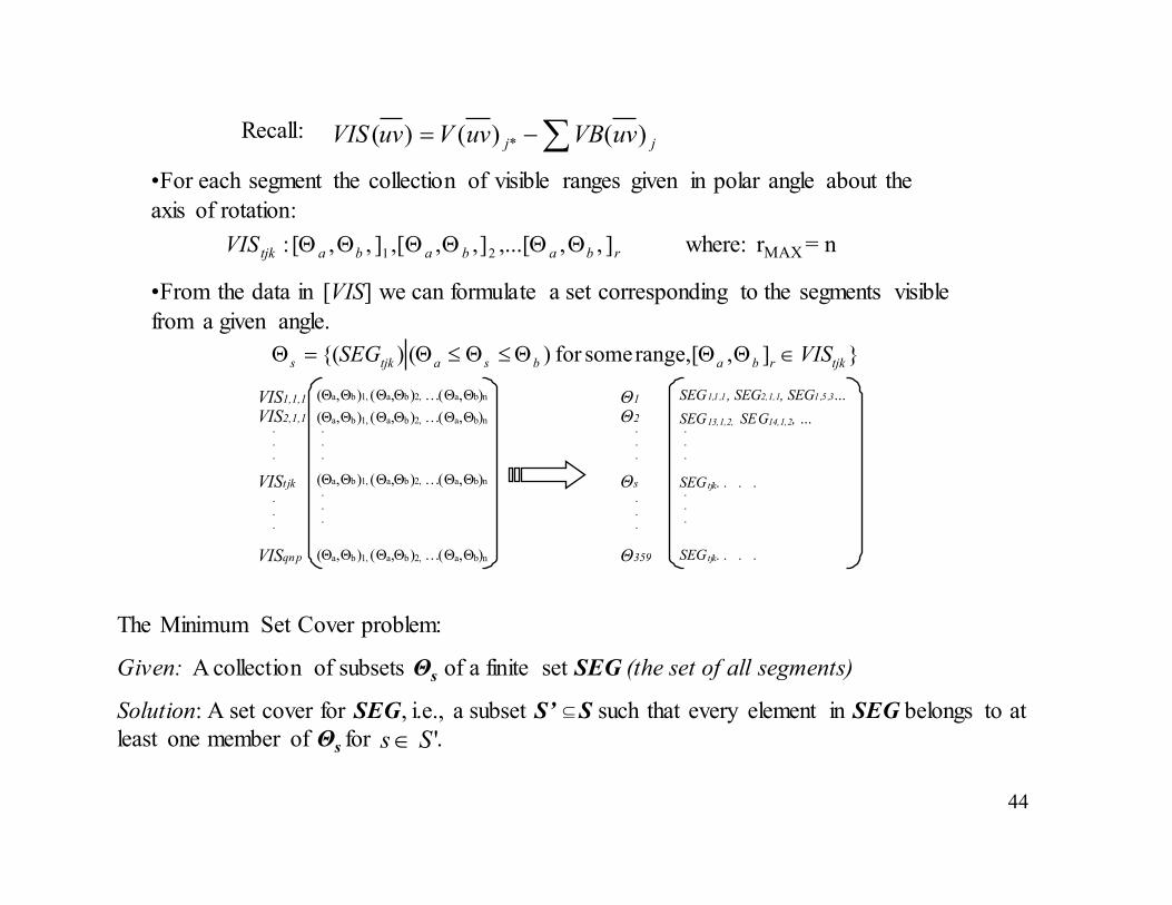
∑−= jj uvVBuvVuvVIS )()()( *Recall:

•For each segment the collection of visible ranges given in polar angle about the

axis of rotation:

rbababatjkVIS ],,,...[],,[,],,[: 21 ΘΘΘΘΘΘ where: rMAX = n

•From the data in [VIS] we can formulate a set corresponding to the segments visible

from a given angle.

}],[ range, somefor )(){( tjkrbabsatjks VISSEG ∈ΘΘΘ≤Θ≤Θ=Θ

.

.

.

VIS1,1,1 VIS2,1,1

VISt jk

VISqn p

.

.

.

(Θa,Θb)1, (Θa,Θb)2, …(Θa,Θb)n

.

.

.

.

.

.

(Θa,Θb)1, (Θa,Θb)2, …(Θa,Θb)n

(Θa,Θb)1, (Θa,Θb)2, …(Θa,Θb)n

(Θa,Θb)1, (Θa,Θb)2, …(Θa,Θb)n

.

.

.

Θ1 Θ2

Θs

Θ359

.

.

.

SEG1,1 ,1, SEG2,1,1, SEG1 ,5 ,3…

.

.

.

.

.

.

SEG13,1,2, SEG14,1,2, …

SEG tjk. . . .

SEG tjk. . . .

The Minimum Set Cover problem:

Given: A collection of subsets Θs of a finite set SEG (the set of all segments)

Solution: A set cover for SEG, i.e., a subset S’ S such that every element in SEG belongs to at

least one member of Θs for .

⊆

'Ss∈

45

Implementation/Results

• Algorithm implemented in C

• Computation times on a 2.0GHz Pentium 4

320º

49º140º

228º

C.H.

A.C.

Facets

Slice ( in ) #sgmts time( s ) #sgmts time(s ) #sgmts time(s ) #sgmts time( s ) #sgmts time( s )

0.0025 19,566 22.750 27,285 25.812 36,199 29.390 49,975 36.623 69,212 47.122

0.0050 9,772 11.230 13,553 12.875 18,178 14.671 25,044 18.640 34,458 23.389

0.0100 4,850 5.687 6,781 6.515 9,054 7.405 12,476 9.297 17,306 11.843

0.0200 2,375 2.875 3,409 3.312 4,597 3.907 6,269 4.859 8,683 6.281

0.0400 1,182 1.453 1,655 1.718 2,159 2.032 2,974 2.453 4,123 3.141

1990 3686

STL Resolution

865

coarse

0.005"

0.5

1286

xcoarse

0.0075"

0.5

6578

medium

0.0025"

0.5

xfine

0.000625"

0.5

0.00125"

fine

0.5

• Set cover problem solved as integer linear program using LINDO:

The “Jack”…

46

xy

z

x y

z

x

x y

z

y

z

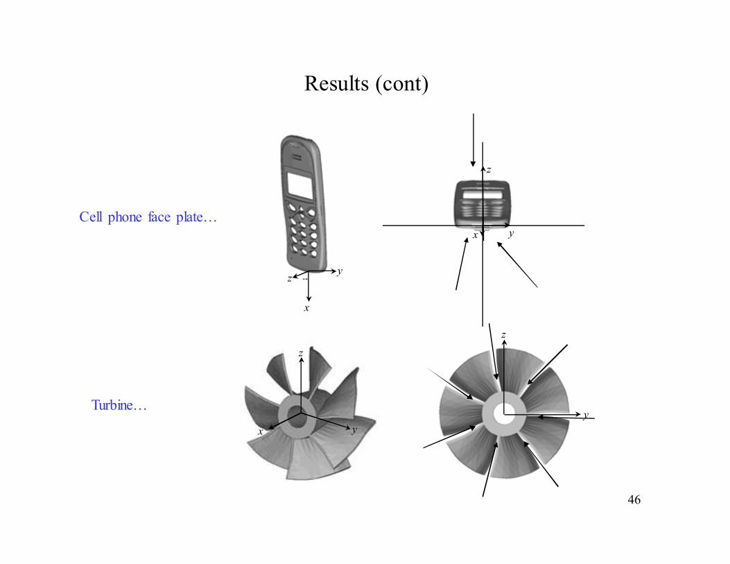
Results (cont)

Cell phone face plate…

Turbine…

47

Toolpath Planning

• Layer based toolpaths

– Machine visible surfaces from approach direction

– 2½-D pocketing, easily generated using current CAM software (MasterCAM,rough surface pocketing)

– A gouge-free approach, given flute and shank diameter are same (or shank < flute)

– Investigated as a rough machining approach - Balasubramanium, 1999

• Can approach finish machining using very small depths of cut

• We assume that tool length, not diameter will be active constraint

– To avoid collision, tool length > maximum swept diameter of part (Same as stock diameter)

– Tool diameter chosen as smallest available for required length (not conventional tools)

48

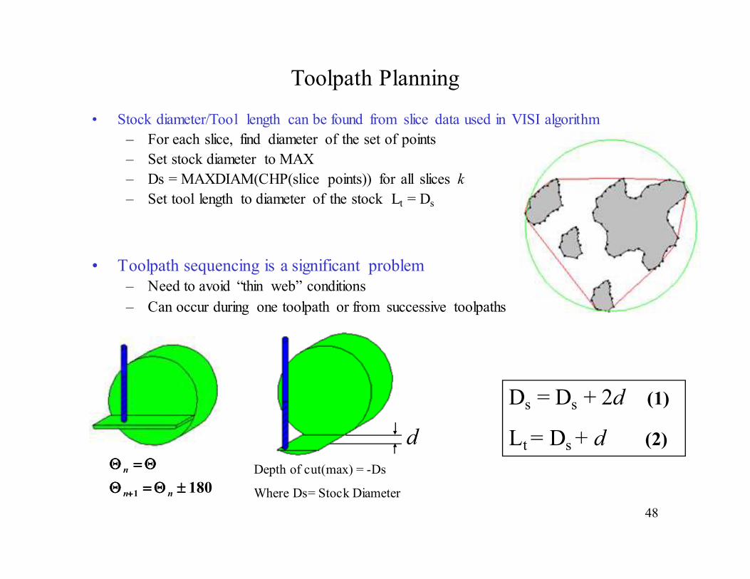
Toolpath Planning

• Stock diameter/Tool length can be found from slice data used in VISI algorithm

– For each slice, find diameter of the set of points

– Set stock diameter to MAX

– Ds = MAXDIAM(CHP(slice points)) for all slices k

– Set tool length to diameter of the stock Lt = Ds

• Toolpath sequencing is a significant problem

– Need to avoid “thin web” conditions

– Can occur during one toolpath or from successive toolpaths

Depth of cut(max) = -Ds

Where Ds= Stock Diameter

d

Ds = Ds + 2d (1)

Lt = Ds + d (2)

1801 ±±±±ΘΘΘΘ====ΘΘΘΘ

ΘΘΘΘ====ΘΘΘΘ

++++ nn

n

49

Toolpath Planning

nΘΘΘΘ

ΘΘΘΘ±±±±±±±±ΘΘΘΘ

ΘΘΘΘ±±±±±±±±ΘΘΘΘ≠≠≠≠ΘΘΘΘ ++++

)180(

)90(1

d

o

n

d

o

n

n

o

dwhere: 10 ====ΘΘΘΘ

(3)

ΘΘΘΘ====ΘΘΘΘn 901 ±±±±ΘΘΘΘ====ΘΘΘΘ ++++ nn

• Thin material conditions resulting from thru-pocket part geometry:

• For each successive toolpath

planned in sequence, undesirable

orientations to be avoided:

50

Toolpath Planning

• Preparatory toolpath sequence to avoid thin material conditions

• Removes bulk of stock material prior to processing remainder of toolpaths

• Choose from orientations in the solution set, or add new

Model

Remaining stock

material

*Preparatory passes adhere to condition: (3)

51

Fixture Planning

• Approach uses “sacrificial supports” to retain the prototype within the stock material

• Round stock clamped between opposing chucks

• As prototype is rotated b/w toolpaths sacrificial supports are incrementally created

• Supports cut away to remove finished part

• Current approach assumes model surfaces exist along axis of rotation

– Only one fixture support cylinder used on each end

– No change to visibility calculations

Problems:

Where do cylinders begin/end?

What diameter?

52

Fixture Planning

• Start/end of cylinder

– Need to have room for tool diameter to pass b/w end of part and stock

– Cylinder end protruding into the part must be fully “embedded”

• Use slice geometry to calculate depth of penetration where cylinder is fully attached

Part length

Lf

Free fixture length: Lf > Dt

Where Dt = diameter of tool

Pd ?Lf

53

Fixture Planning• Determine first slice where fixture cylinder diameter is contained within the boundary

chain of the part ( Circle with center at axis of rotation )

Slice k=1 (0.005”) Slice k=1 (0.010”) Slice k=1 (0.015”)

Part slice boundary

Fixture cylinder diameter

*

Pd = 0.015”

54

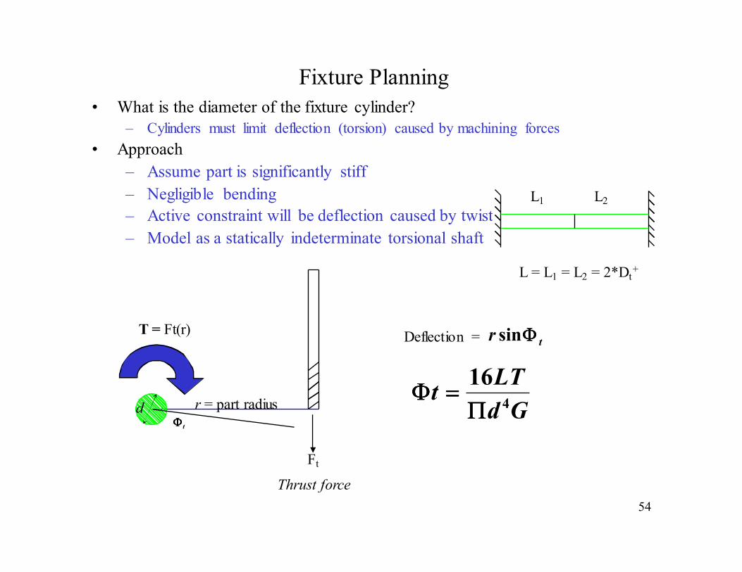
Fixture Planning

• What is the diameter of the fixture cylinder?

– Cylinders must limit deflection (torsion) caused by machining forces

• Approach

– Assume part is significantly stiff

– Negligible bending

– Active constraint will be deflection caused by twisting

– Model as a statically indeterminate torsional shaft

Ft

r = part radius

T = Ft(r)tr ΦΦΦΦsin

tΦΦΦΦsin

Deflection =

d

L1 L2

L = L1 = L2 = 2*Dt+

Thrust force

Gd

LTt

4

16

ΠΠΠΠ====ΦΦΦΦ

55

Fixture Planning• Fixture setup:

– Straightforward to determine work offset location, length of stock

– Ensures collision avoidance Dh

b a

c

a = clamping depth

b = .5Dh - .5(Dt) work offset from jaw face

c = Lp + 2a + 2b + 2Lf

Where: Dh = tool holder diameter, Dt = tool diameter, Lf = free fixture length, Lp = Part length

56

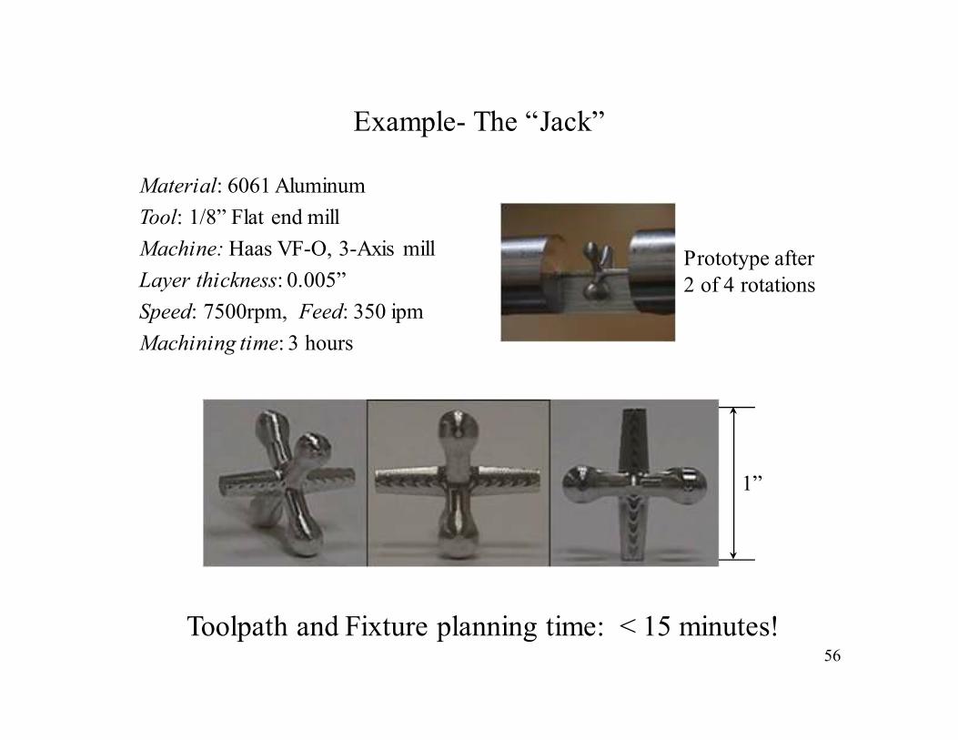
Example- The “Jack”

1”

Material: 6061 Aluminum

Tool: 1/8” Flat end mill

Machine: Haas VF-O, 3-Axis mill

Layer thickness: 0.005”

Speed: 7500rpm, Feed: 350 ipm

Machining time: 3 hours

Prototype after

2 of 4 rotations

Toolpath and Fixture planning time: < 15 minutes!

57

58

59

60

61

62

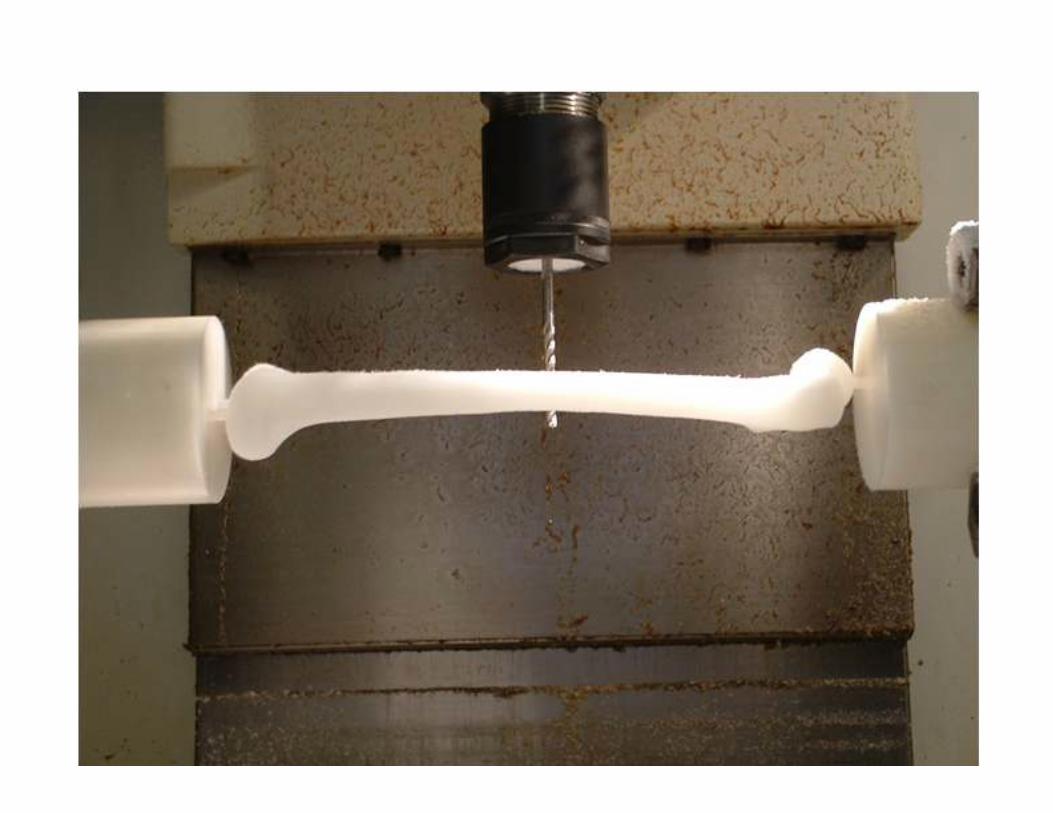
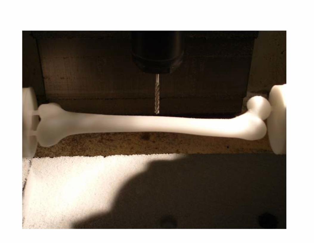
• Medical RP, one of the major territories for RP application

– Manufacturing of dimensionally accurate physical models of the human anatomy derived from medical image data using a variety of rapid prototyping (RP) technologies

– CNC-RP?

• Typical bio/medical Material

– Titanium

– Stainless steel

– Cobalt alloy

• Advantage of Wire Electric Discharge Machining(WEDM)

– Cut any electrical conductive material regardless hardness

– Ignorable cutting force

– Capable to produce complex part

Satisfy material requirementSatisfy material requirement

Wire EDM Rapid Prototyping

63

• WEDM is different from traditional

machining process

Point contact

• Wire EDM

• Laser

• Waterjet

Linear Surface

64

• Visibility problems are different

– “Can we see it” vs. “Can we access it using a

straight line”

Can we see it?

Tool orientation

Can we access it?

wire orientation

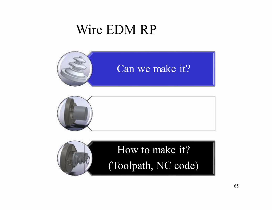
65

Can we make it?

How to make it?

(setup)

How to make it?

(Toolpath, NC code)

Wire EDM RP

66

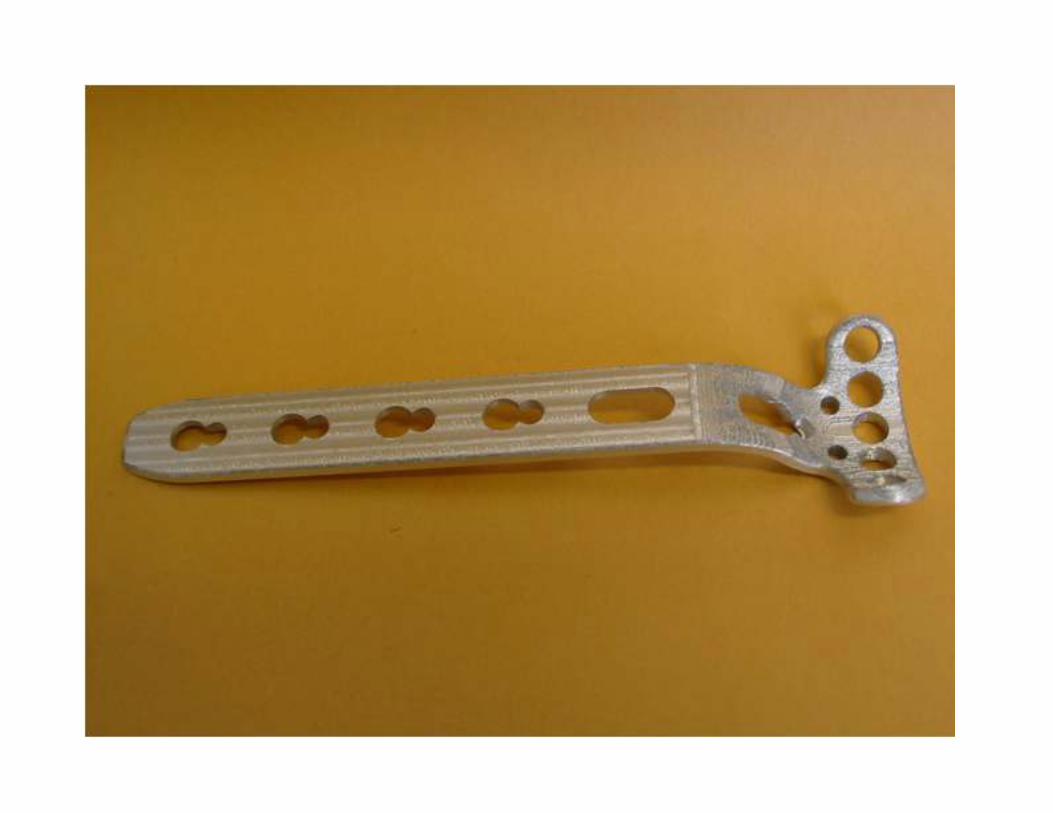
• Investigate the manufacturability

– Part Geometry

– 6-axis Wire EDM

– Rigid machining part

– No internal through features

• Find the B-axis orientation

– Try to minimize number of B-axis orientation

Can we make it?

How to make it?

(setup)

Wire EDM RP

67

• Toolpath generation

– Discrete Toolpath for B-axis and other 5-axis

– STEP-NC

• Fixture Design

– Ignorable cutting force : Clamp part

How to make it?

(Toolpath, NC code)

Wire EDM RP

68

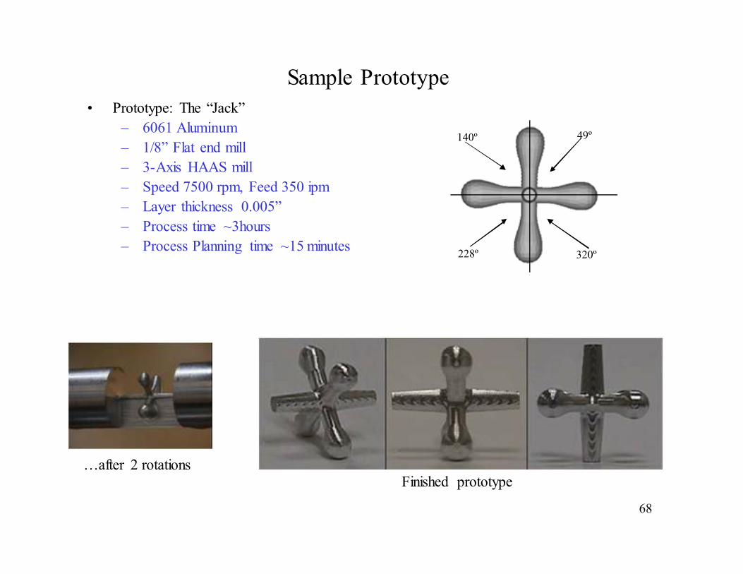
Sample Prototype

• Prototype: The “Jack”

– 6061 Aluminum

– 1/8” Flat end mill

– 3-Axis HAAS mill

– Speed 7500 rpm, Feed 350 ipm

– Layer thickness 0.005”

– Process time ~3hours

– Process Planning time ~15 minutes

…after 2 rotationsFinished prototype

320º

49º140º

228º

6969

Conclusions

• For prototyping, the process is dominated by engineering

cost

– Product engineering, Process engineering, production engineering

• RP has come a long way

– Usable products

– Process and production engineering coasts are minimal

• Conventional methods are on their way back

– CNC RP

– Wire EDM RP

70

Conclusions -- continued

• The methods developed (CNC-RP and Wire EDM –RP) represent a deliberate approach at making CNC machining usable by engineers and designers, not just machinists

• Capable of producing fully functional prototypes in the appropriate material

• Wide spread availability of CNC machines provides fast, low-cost integration to current product design processes

• Quick changeover from RP to Production setup will enable higher utilization of machines

• The concept of sacrificial supports for CNC machining represents a significant area of basic research that may yield even greater contributions outside of RP

71

References:

• Wang, F.C., L. Marchetti, P.K. Wright, “Rapid Prototyping Using Machining”, SME Technical

Paper, PE99-118, 1999

• Chen, Y.H., Song, Y., “The development of a layer based machining system”, Computer Aided

Design, Vol. 33, pp. 331-342, 2001

• Merz, R., Prinz, F.B., Ramaswami, K., Terk, M., Weiss, L.E., “Shape Deposition Manufacturing”,

Proceedings of the Solid Freeform Fabrication Symposium, University of Texas at Austin, pp. 1-8,

1994

• Walczyk, D.F., Hardt, D.E., “Rapid tooling for sheet metal forming using profiled edge laminations-

design principles and demonstration”, Journal of Manufacturing Science and Engineering,

Transactions of the ASME, Vol. 120, No. 2, pp. 746-754, November 1998

• Vouzelaud, F.A., Bagchi, A. & Sferro, P.F., (1992), Adaptive Laminated Machining for Prototyping

of Dies and Molds, Proceedings of the 3rd Solid Freeform Fabrication Symposium, pp. 291-300,

August 1992

• Lennings, L., “Selecting Either Layered manufacturing or CNC machining to build your prototype”,

SME Technical Paper, Rapid Prototyping Association, PE00-171, 2000

• Peshkin, M.A., Sanderson, A.C., “Reachable Grasps on a Polygon: The Convex Rope Algorithm”,

IEEE Journal of Robotics and Automation, Vol. RA-2, No. 1, March 1986

• Lee, D. T., Preparata, F. P., "Euclidean Shortest Paths in the Presence of rectilinear Barriers",

Networks, Vol. 14, No. 3, pp. 393-410, 1984.

• Stewart, J.A., “Computing visibility from folded surfaces”, Computers and Graphics, Vol. 23, No. 5,

pp. 693-702, 1999

• Balasubramaniam, M., “Tool Selection and Path Planning for 3-Axis Rough Cutting”, Thesis,

Department of Mechanical Engineering, The Massachusetts Institute of Technology, June 1999

• Tang, K., Woo, T.C., Gan, J., “Maximum Intersection of Spherical Polygons and Workpiece

Orientation for 4- and 5-Axis Machining”, Journal of Mechanical Design, Vol. 114, pp. 477-485,

September 1992