cmsc 341

CMSC 341 Asymptotic Anaylsis 1

CMSC 341

Asymptotic Analysis


Complexity How many resources will it take to solve a

problem of a given size? time space

Expressed as a function of problem size (beyond some minimum size) how do requirements grow as size grows?

Problem size number of elements to be handled size of thing to be operated on


The Goal of Asymptotic Analysis How to analyze the running time (aka computational

complexity) of an algorithm in a theoretical model. Using a theoretical model allows us to ignore the

effects of Which computer are we using? How good is our compiler at optimization

We define the running time of an algorithm with input size n as T ( n ) and examine the rate of growth of T( n ) as n grows larger and larger and larger.


Growth Functions

ConstantT(n) = cex: getting array element at known location

any simple C++ statement (e.g. assignment) Linear

T(n) = cn [+ possible lower order terms]ex: finding particular element in array of size n

(i.e. sequential search)trying on all of your n shirts


Growth Functions (cont.)

QuadraticT(n) = cn2 [ + possible lower order terms]ex: sorting all the elements in an array (using bubble sort) trying all your n shirts with all your n ties

PolynomialT(n) = cnk [ + possible lower order terms]ex: finding the largest element of a k-dimensional arraylooking for maximum substrings in array


Growth Functions (cont.)

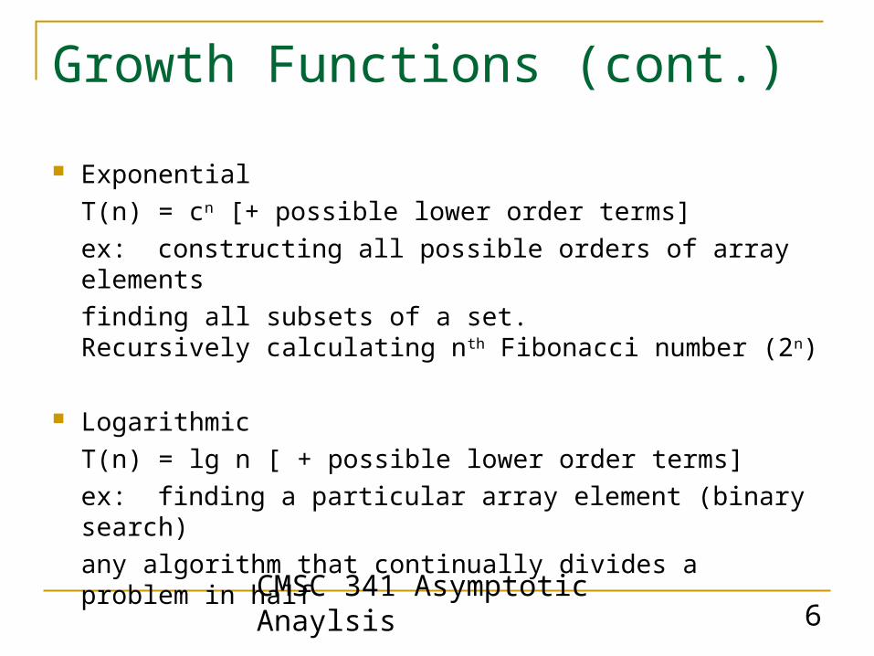
ExponentialT(n) = cn [+ possible lower order terms]ex: constructing all possible orders of array elements

finding all subsets of a set.Recursively calculating nth Fibonacci number (2n)

LogarithmicT(n) = lg n [ + possible lower order terms]ex: finding a particular array element (binary search)any algorithm that continually divides a problem in half


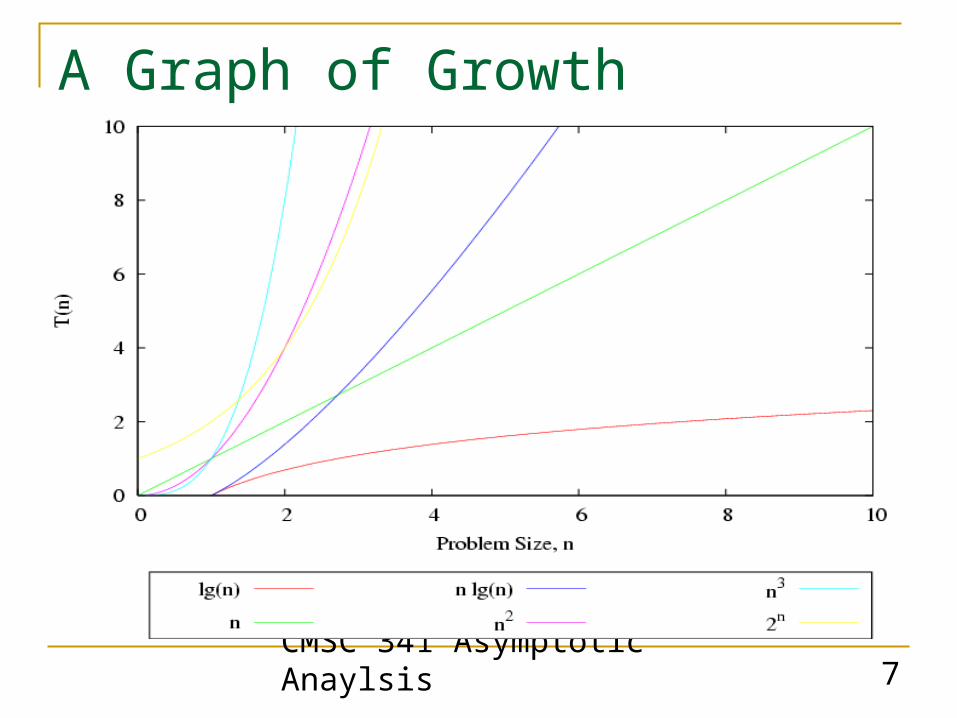
A Graph of Growth Functions


Expanded Scale


Asymptotic Analysis

How does the time (or space) requirement grow as the problem size grows really, really large? We are interested in “order of magnitude” growth rate. We are usually not concerned with constant

multipliers. For instance, if the running time of an algorithm is proportional to (let’s suppose) the square of the number of input items, i.e. T(n) is c*n2, we won’t (usually) be concerned with the specific value of c.

Lower order terms don’t matter.


Definition of Big-Oh

T(n) = O(f(n)) (read “T( n ) is in Big-Oh of f( n )” )if and only if T(n) cf(n) for some constants c, n0 and n n0

This means that eventually (when n n0 ), T( n ) is always less than or equal to c times f( n ).

The growth rate of T(n) is less than or equal to that of f(n)Loosely speaking, f( n ) is an “upper bound” for T ( n )

NOTE: if T(n) =O(f(n)), there are infinitely many pairs of c’s and n0

’s that satisfy the relationship. We only need to find one such pair for the relationship to hold.


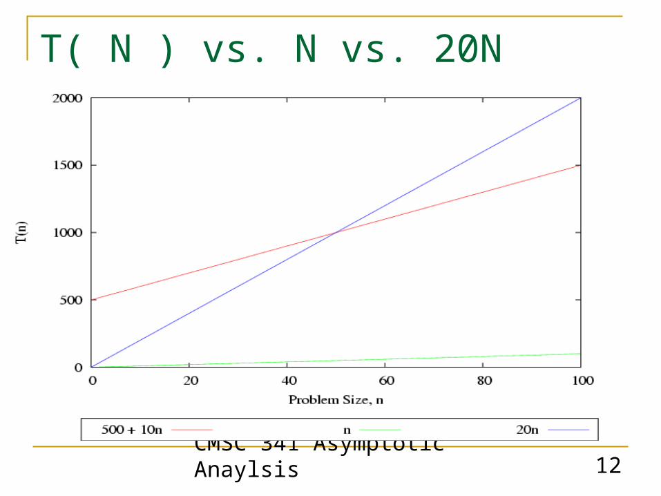
Big-Oh Example Suppose we have an algorithm that reads N integers from

a file and does something with each integer. The algorithm takes some constant amount of time for

initialization (say 500 time units) and some constant amount of time to process each data element (say 10 time units).

For this algorithm, we can say T( N ) = 500 + 10N. The following graph shows T( N ) plotted against N, the

problem size and 20N. Note that the function N will never be larger than the

function T( N ), no matter how large N gets. But there are constants c0 and n0 such that T( N ) <= c0N when N >= n0, namely c0 = 20 and n0 = 50.

Therefore, we can say that T( N ) is in O( N ).


T( N ) vs. N vs. 20N


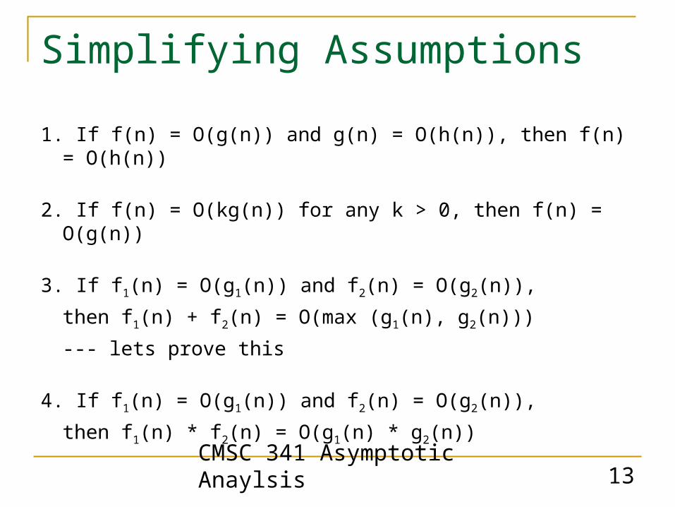
Simplifying Assumptions

1. If f(n) = O(g(n)) and g(n) = O(h(n)), then f(n) = O(h(n))

2. If f(n) = O(kg(n)) for any k > 0, then f(n) = O(g(n))

3. If f1(n) = O(g1(n)) and f2(n) = O(g2(n)),

then f1(n) + f2(n) = O(max (g1(n), g2(n)))

--- lets prove this

4. If f1(n) = O(g1(n)) and f2(n) = O(g2(n)),

then f1(n) * f2(n) = O(g1(n) * g2(n))


Sum in Bounds (the “sum rule”) Theorem:

Let T1(n) = O(f(n)) and T2(n) = O(g(n)).

Then T1(n) + T2(n) = O(max (f(n), g(n))).

Proof: From the definition of O,

T1(n) c1f (n) for n n1 and T2(n) c2g(n) for n n2

Let n0 = max(n1, n2). Then, for n n0, T1(n) + T2(n) c1f (n) + c2g(n) Let c3 = max(c1, c2). Then, T1(n) + T2(n) c3 f (n) + c3 g (n) 2c3 max(f (n), g (n))

c max(f (n), g (n)) = O (max (f(n), g(n)))


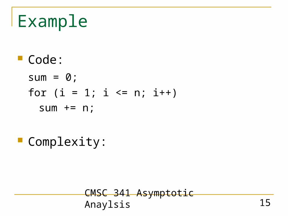
Example

Code:sum = 0;for (i = 1; i <= n; i++)sum += n;

Complexity:


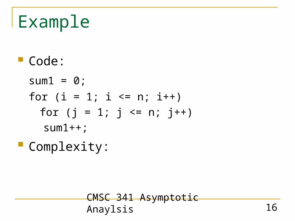
Example

Code:sum1 = 0;for (i = 1; i <= n; i++)for (j = 1; j <= n; j++)sum1++;

Complexity:


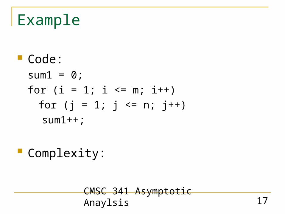
Example

Code:sum1 = 0;for (i = 1; i <= m; i++)for (j = 1; j <= n; j++)sum1++;

Complexity:


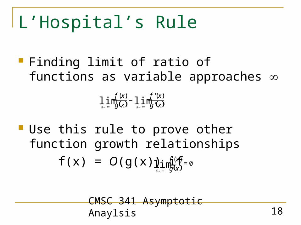
L’Hospital’s Rule

Finding limit of ratio of functions as variable approaches

Use this rule to prove other function growth relationships

f(x) = O(g(x)) if

( ) ( )xgxf

xgxf

xx ')(')( limlim

∞→∞→=

( ) 0)(lim =∞→ xg

xfx


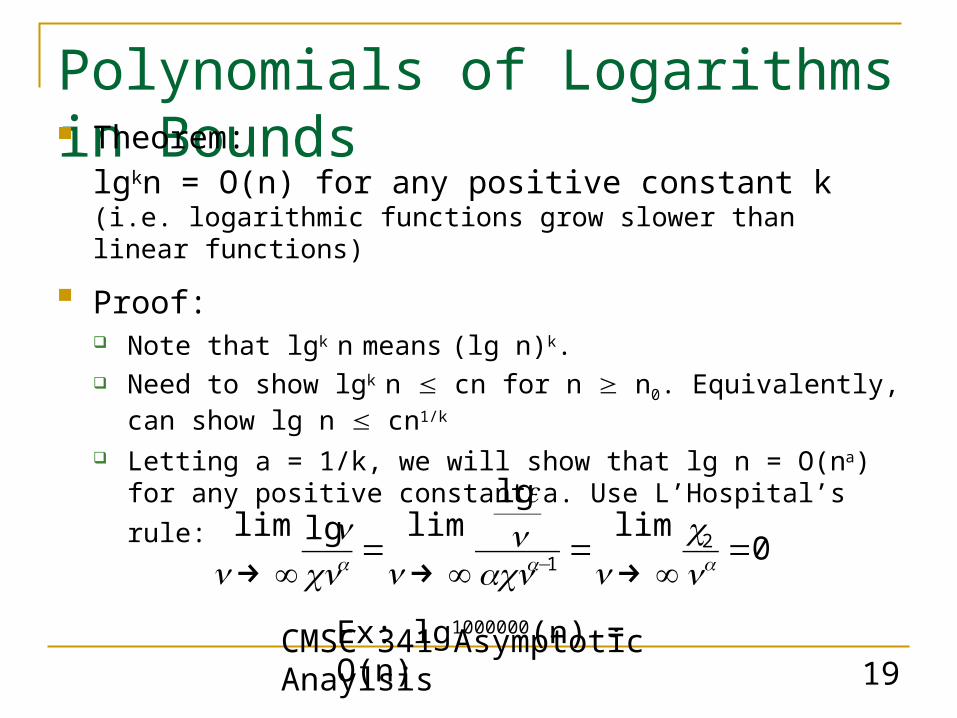
Polynomials of Logarithms in Bounds Theorem:

lgkn = O(n) for any positive constant k(i.e. logarithmic functions grow slower than linear functions)

Proof: Note that lgk n means (lg n)k. Need to show lgk n cn for n n0. Equivalently, can show lg n

cn1/k

Letting a = 1/k, we will show that lg n = O(na) for any positive constant a. Use L’Hospital’s rule:

0lim

lglimlglim 2

1 =∞→

=∞→

=∞→ − aaa n

cnacn

ne

ncnn

n

Ex: lg1000000(n) = O(n)


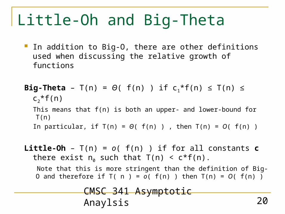
Little-Oh and Big-Theta In addition to Big-O, there are other definitions used

when discussing the relative growth of functions

Big-Theta – T(n) = Θ( f(n) ) if c1*f(n) ≤ T(n) ≤ c2*f(n)This means that f(n) is both an upper- and lower-bound for T(n)In particular, if T(n) = Θ( f(n) ) , then T(n) = O( f(n) )

Little-Oh – T(n) = o( f(n) ) if for all constants c there exist n0 such that T(n) < c*f(n). Note that this is more stringent than the definition of Big-O and therefore if T( n ) = o( f(n) ) then T(n) = O( f(n) )


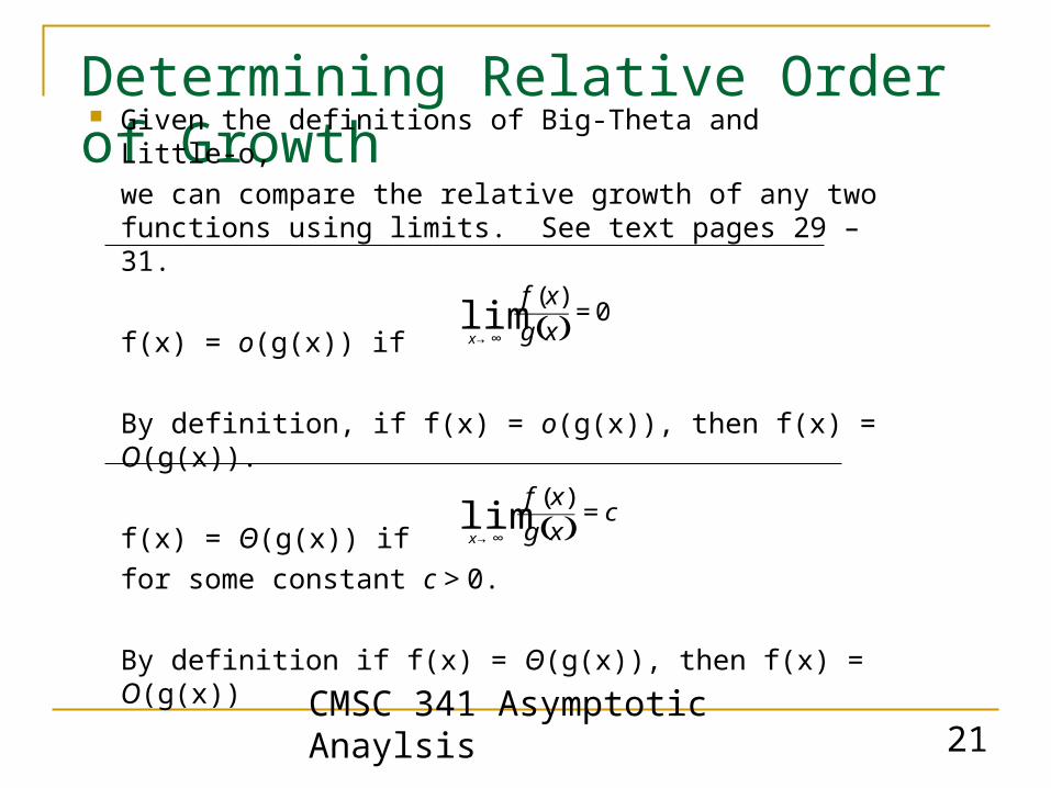
Determining Relative Order of Growth Given the definitions of Big-Theta and Little-o,

we can compare the relative growth of any two functions using limits. See text pages 29 – 31.

f(x) = o(g(x)) if

By definition, if f(x) = o(g(x)), then f(x) = O(g(x)).

f(x) = Θ(g(x)) iffor some constant c > 0.

By definition if f(x) = Θ(g(x)), then f(x) = O(g(x))

( ) 0)(lim =∞→ xg

xfx

( ) cxgxf

x=

∞→

)(lim


Space Complexity

Does it matter?

What determines space complexity?

How can you reduce it?

What tradeoffs are involved?


Appendix


Example

Square each element of an N x N matrix

Printing the first and last row of an N x N matrix

Finding the smallest element in a sorted array of N integers

Printing all permutations of N distinct elements


Constants in Bounds(“constants don’t matter”) Theorem:

If T(x) = O(cf(x)), then T(x) = O(f(x)) Proof:

T(x) = O(cf(x)) implies that there are constants c0 and n0 such that T(x) c0(cf(x)) when x n0

Therefore, T(x) c1(f(x)) when x n0 where c1 = c0c

Therefore, T(x) = O(f(x))


Products in Bounds (“the product rule”) Theorem:

Let T1(n) = O(f(n)) and T2(n) = O(g(n)).

Then T1(n) * T2(n) = O(f(n) * g(n)). Proof:

Since T1(n) = O(f(n)), then T1 (n) c1f(n) when n n1

Since T2(n) = O(g(n)), then T2 (n) c2g(n) when n n2

Hence T1(n) * T2(n) c1 * c2 * f(n) * g(n) when n n0

where n0 = max (n1, n2) And T1(n) * T2(n) c * f (n) * g(n) when n n0

where n0 = max (n1, n2) and c = c1*c2

Therefore, by definition, T1(n)*T2(n) = O(f(n)*g(n)).


Polynomials in Bounds

Theorem: If T (n) is a polynomial of degree k, then T(n) = O(nk).

Proof: T (n) = nk + nk-1 + … + c is a polynomial of degree k. By the sum rule, the largest term dominates. Therefore, T(n) = O(nk).


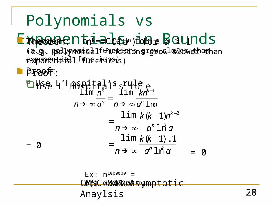
Polynomials vs Exponentials in Bounds Theorem: nk = O(an) for a > 1

(e.g. polynomial functions grow slower than exponential functions) Proof:

Use L’Hospital’s rule

= 0

aakn

nan

n n

k

n

k

lnlimlim 1−

∞→=

∞→

aankk

n n

k

2

2

ln)1(lim −−

∞→=

aakk

n kn ln1)...1(lim −

∞→=

Ex: n1000000 = O(1.00000001n)

Theorem: nk = O(an) for a > 1(e.g. polynomial functions grow slower than exponential functions)

Proof: Use L’Hospital’s rule

= 0aa

kkn kn ln

1)...1(lim −∞→

=


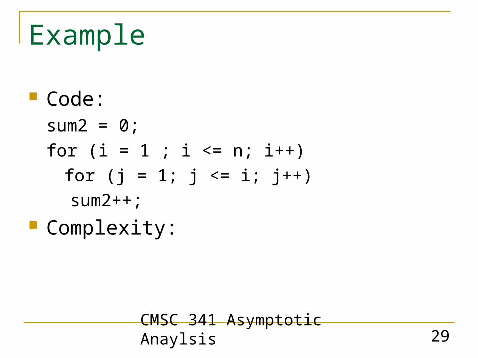
Example

Code: sum2 = 0;for (i = 1 ; i <= n; i++)for (j = 1; j <= i; j++)sum2++;

Complexity:


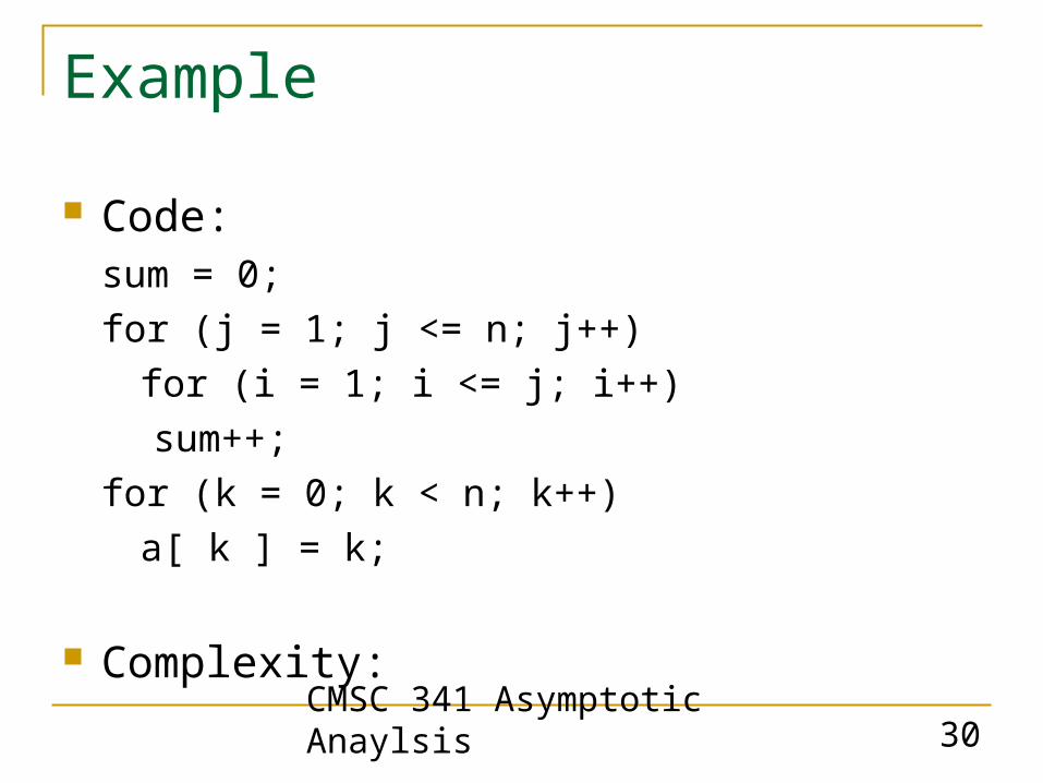
Example

Code:sum = 0;for (j = 1; j <= n; j++)for (i = 1; i <= j; i++)sum++;

for (k = 0; k < n; k++)a[ k ] = k;

Complexity:


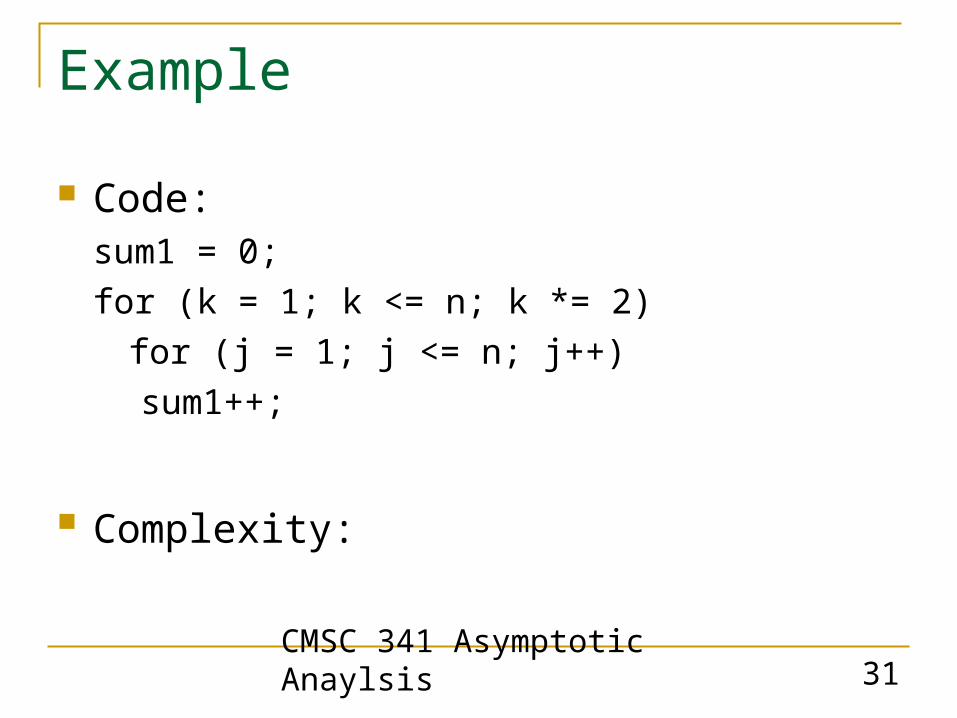
Example

Code:sum1 = 0;for (k = 1; k <= n; k *= 2)for (j = 1; j <= n; j++)sum1++;

Complexity:


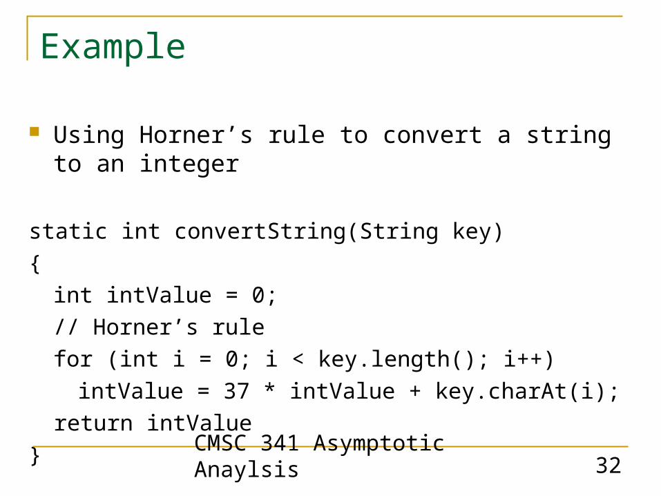
Example

Using Horner’s rule to convert a string to an integer

static int convertString(String key){int intValue = 0;// Horner’s rulefor (int i = 0; i < key.length(); i++)intValue = 37 * intValue + key.charAt(i);

return intValue}


Determining relative order of Growth Often times using limits is unnecessary as simple

algebra will do. For example, if f(n) = n log n and g(n) = n1.5 then deciding

which grows faster is the same as determining which of f(n) = log n and g(n) = n0.5 grows faster (after dividing both functions by n), which is the same as determining which of f(n) = log2 n and g(n) = n grows faster (after squaring both functions). Since we know from previous theorems that n (linear functions) grows faster than any power of a log, we know that g(n) grows faster than f(n).


Big-Oh is not the whole story

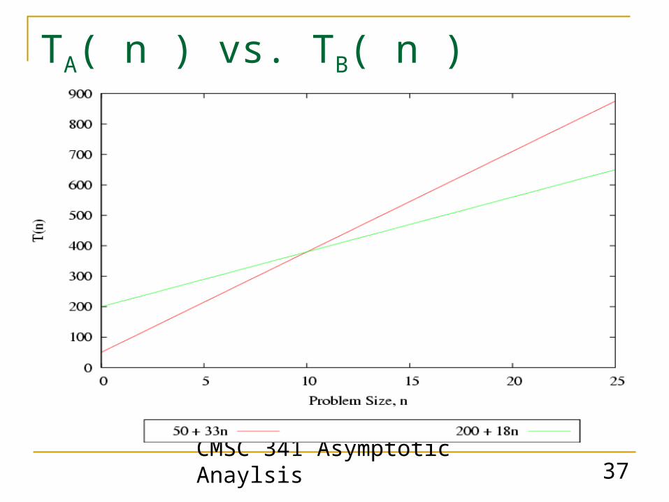
Suppose you have a choice of two approaches to writing a program. Both approaches have the same asymptotic performance (for example, both are O(n lg(n)). Why select one over the other, they're both the same, right? They may not be the same. There is this small matter of the constant of proportionality.

Suppose algorithms A and B have the same asymptotic performance, TA(n) = TB(n) = O(g(n)). Now suppose that A does 10 operations for each data item, but algorithm B only does 3. It is reasonable to expect B to be faster than A even though both have the same asymptotic performance. The reason is that asymptotic analysis ignores constants of proportionality.

The following slides show a specific example.


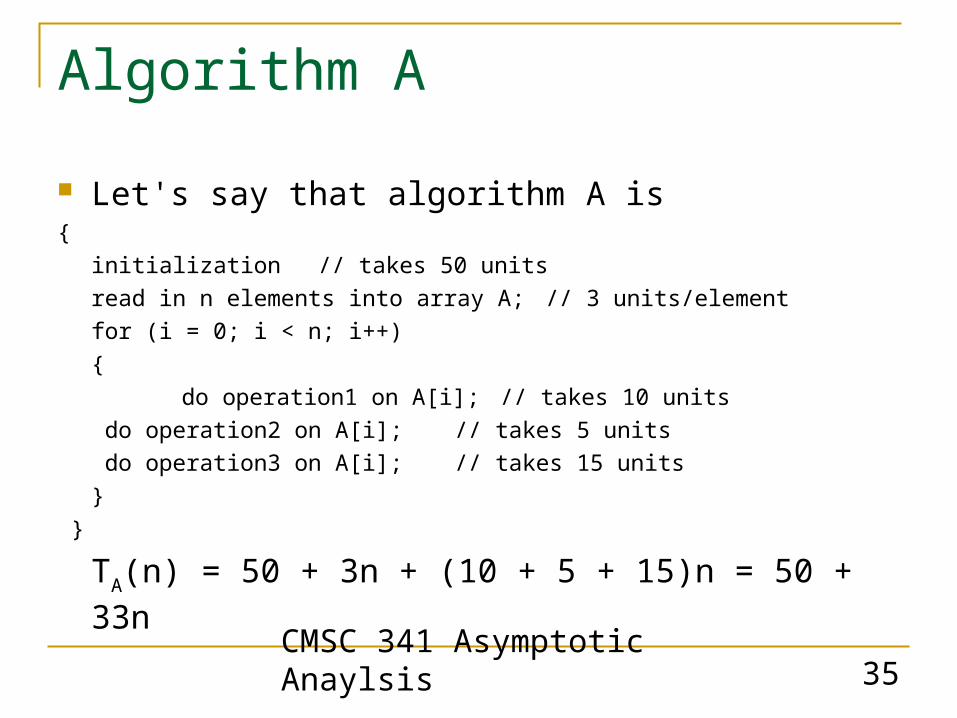
Algorithm A

Let's say that algorithm A is {

initialization // takes 50 unitsread in n elements into array A; // 3 units/elementfor (i = 0; i < n; i++) { do operation1 on A[i]; // takes 10 units

do operation2 on A[i]; // takes 5 units do operation3 on A[i]; // takes 15 units

} }

TA(n) = 50 + 3n + (10 + 5 + 15)n = 50 + 33n


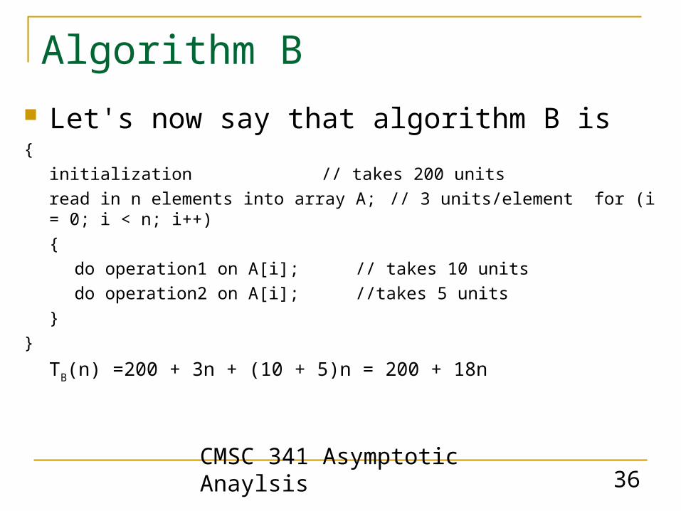
Algorithm B Let's now say that algorithm B is {

initialization // takes 200 unitsread in n elements into array A; // 3 units/element for (i = 0; i < n; i++){

do operation1 on A[i]; // takes 10 unitsdo operation2 on A[i]; //takes 5 units

}}

TB(n) =200 + 3n + (10 + 5)n = 200 + 18n


TA( n ) vs. TB( n )


A concrete example

N T(n) = n T(n) = nlgn T(n) = n2 T(n) = n3 Tn = 2n

5 0.005 s 0.01 s 0.03 s 0.13 s 0.03 s

10 0.01 s 0.03 s 0.1 s 1 s 1 s

20 0.02 s 0.09 s 0.4 s 8 s 1 ms

50 0.05 s 0.28 s 2.5 s 125 s 13 days

100 0.1 s 0.66 s 10 s 1 ms 4 x 1013 years

The following table shows how long it would take to perform T(n) steps on a computer that does 1 billion steps/second. Note that a microsecond is a millionth of a second and a millisecond is a thousandth of a second.

Notice that when n >= 50, the computation time for T(n) = 2n has started to become too large to be practical. This is most certainly true when n >= 100. Even if we were to increase the speed of the machine a million-fold, 2n for n = 100 would be 40,000,000 years, a bit longer than you might want to wait for an answer.


Amortized Analysis

Sometimes the worst-case running time of an operation does not accurately capture the worst-case running time of a sequence of operations.

What is the worst-case running time of ArrayList’s add( ) method that places a new element at the end of the ArrayList?

The idea of amortized analysis is to determine the average running time of the worst case.


Amortized Example – add() In the worst case, there is no room in the ArrayList for the new element,

X. The ArrayList then doubles its current size, copies the existing elements into the new ArrayList, then places X in the next available slot. This operation is O( N ) where N is the current number of elements in the ArrayList.

But this doubling happens very infrequently. (how often?) If there is room in the ArrayList for X, then it is just placed in the next

available slot in the ArrayList and no doubling is required. This operation is O( 1 ) – constant time

To discuss the running time of add( ) it makes more sense to look at a long sequence of add( ) operations rather than individual operations since not all individual operations

A sequence of N add( ) operations can always be done in O(N), so we say the amortized running time of per add( )operation is O(N) / N = O(1) or constant time.

We are willing to perform a very slow operation (doubling the vector size) very infrequently in exchange for frequently having very fast operations.


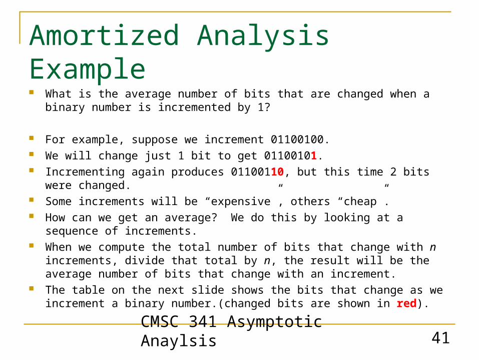
Amortized Analysis Example What is the average number of bits that are changed when a binary number

is incremented by 1?

For example, suppose we increment 01100100. We will change just 1 bit to get 01100101. Incrementing again produces 01100110, but this time 2 bits were changed. Some increments will be “expensive”, others “cheap”. How can we get an average? We do this by looking at a sequence of

increments. When we compute the total number of bits that change with n increments,

divide that total by n, the result will be the average number of bits that change with an increment.

The table on the next slide shows the bits that change as we increment a binary number.(changed bits are shown in red).


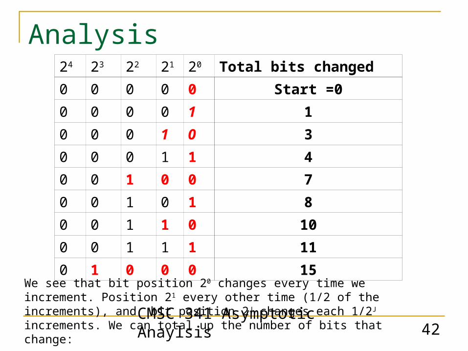
Analysis24 23 22 21 20 Total bits changed0 0 0 0 0 Start =00 0 0 0 1 10 0 0 1 0 30 0 0 1 1 40 0 1 0 0 70 0 1 0 1 80 0 1 1 0 100 0 1 1 1 110 1 0 0 0 15

We see that bit position 20 changes every time we increment. Position 21 every other time (1/2 of the increments), and bit position 2J changes each 1/2J increments. We can total up the number of bits that change:


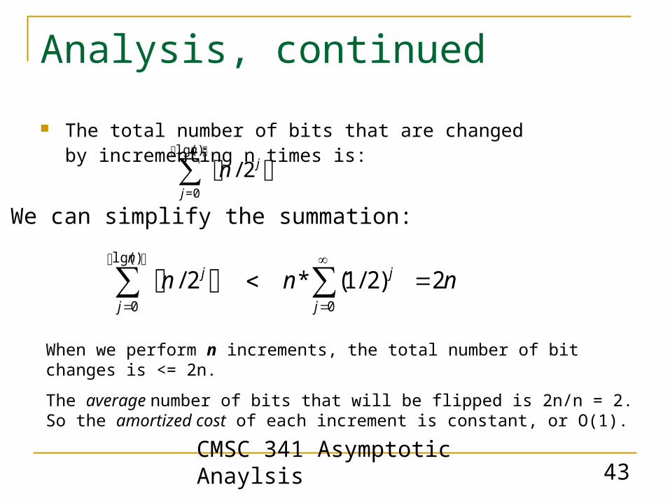
Analysis, continued The total number of bits that are changed by incrementing

n times is: ⎣ ⎦⎣ ⎦jn

j

n 2/)lg(

0∑

=

When we perform n increments, the total number of bit changes is <= 2n.

The average number of bits that will be flipped is 2n/n = 2. So the amortized cost of each increment is constant, or O(1).

⎣ ⎦⎣ ⎦∑∑∞

==

=<0

)lg(

0

2)2/1(*2/j

jn

j

j nnn

We can simplify the summation:

cmsc 341

Documents

asymptotic anaylsiscmsc

asymptotic analysiscmsc

array of size n

goal of asymptotic analysishow

n tiespolynomialtn

n shirtscmsc

input size n

t n note