1    

CMB Fluctuation Dependence on Matter and Dark Energy Density Fraction

Sampanna Pokhrel, Daniel M. Smith, Jr., South Carolina State University, dsmith@scsu.edu

Introduction

The early structure of the universe as seen in the Cosmic Microwave Background (CMB) can be represented by an angular power spectrum (as in Figure 1), a plot that shows how the temperature in the young universe varies over smaller and smaller patches of the sky.

A power spectrum is a very good way to understand and calculate various cosmological parameters related to the universe, and this anisotropy spectrum depends on these parameters. We should first become familiar with the cosmological terms used. For the symbols below, fractional means that the density is divided by the critical matter-energy density for a flat universe, about 10–29g/cm3.

Ωk = curvature parameter Ωcdm = fractional dark matter density Ωb = fractional baryon density ΩΛ = fractional dark energy density H0= Hubble constant = (100km/s/Mpc)h, h is called the Hubble parameter; current best h ≈ 0.7

Figure 1. Angular power spectrum of CMB temperature fluctuations. Plot of temperature fluctuation vs. l-value (a measure of angular scale).

2    

The vertical axis in the diagram above shows the temperature fluctuation and the horizontal axis shows the l-value of the spectrum. The l-value is related to the angular scale of fluctuations. In the table below fill in the l-value and the corresponding angular scale.

First peak Second peak Third peak l-value at spectrum peak (180°/l)= angular scale of fluctuations

Question 1. What happens to the angular scale of the temperature fluctuation when the l-value is increased? ____________________________________________________________________________________

The Big Bang Theory that explains the creation, contents, and evolution of the universe is a scientific theory, a theory that can be proved wrong. The overwhelming evidence, however, is that the theory is a correct description of the universe. In the very early universe there were no atoms; charged electrons and protons scattered light continuously as the universe expanded and cooled. Eventually, 380,000 years after the Big Bang, the universe cooled enough for neutral atoms (H and He) to form and light no longer scattered. But light that scattered just as the neutral atoms were formed continued travel, virtually unimpeded, and it is observed today as microwaves of temperature 2.7 K (– 454.8°F) along with the temperature fluctuations (~10-5) due to the scattering. Studying the temperature fluctuations help to draw conclusions about the shape and contents of the universe.

Early Universe Contents Using 2012 Wilkinson Microwave Anisotropy Probe (WMAP) data, cosmologists find that about 4.6% of the universe is made up of visible matter, i.e. electrons, protons and neutrons. The rest of the 95.4% of the universe is made up of dark matter and dark energy. About 24% of the universe is made up of dark matter and 71.4% is made up of dark energy. Photons (particles of light) and neutrinos (almost massless particles) comprise less than 1% of the universe. Dark matter is a form of matter that is invisible but is observed as the gravitational force needed to hold together galaxy clusters. Dark matter is weakly interacting at best, so once dark matter collapses due to gravitational attraction, it does not generate collisions, heat, or pressure; it stays in place. Until 47,000 years after the Big Bang, radiation was the dominant form of energy. Then matter became the dominant form of energy until 9 billion years after the Big Bang when dark energy dominated over matter. Dark energy is a form of energy that cannot be seen and produces force that opposes gravity and is the cause of the accelerating expansion of the universe. In this lab we ignore the dark energy because the universe was matter dominated when neutral atoms were formed. Early Universe Physics The power spectrum tells us about temperature fluctuations of the young universe. The power spectrum observed today is from the time when matter dominated the universe. In any given volume of space, there

3    

was more energy in the form of matter than in the form of radiation or dark energy. The CMB tells us about the matter density of the early universe. Matter in the form of protons and neutrons are called baryons. (To simplify early universe terminology, electrons are also called baryons by cosmologists although, technically speaking, they are not because of their small mass.) Very soon after the universe begins expansion, dark matter begins to cluster and attract baryons and photons gravitationally. The baryon clustering is opposed by photon pressure pushing the baryons away from the dark matter. The alternate compression and expansion cause the baryon-photon mixture to oscillate just as the alternate compression and expansion of air oscillates to create a sound wave. But the baryon-photon oscillation is better described as an acoustic wave, since no sound is created.

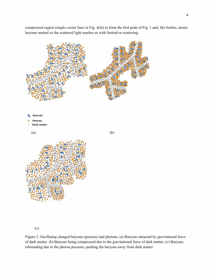
In the diagrams below, Fig. 2(a) shows the baryons being attracted towards dark matter due to gravity. Fig. 2(b) shows the baryons being compressed as photon pressure builds to push them away from dark matter. Fig.2(c) shows the baryons expanding away from the dark matter. The expansion is due to photons pushing the baryons away.

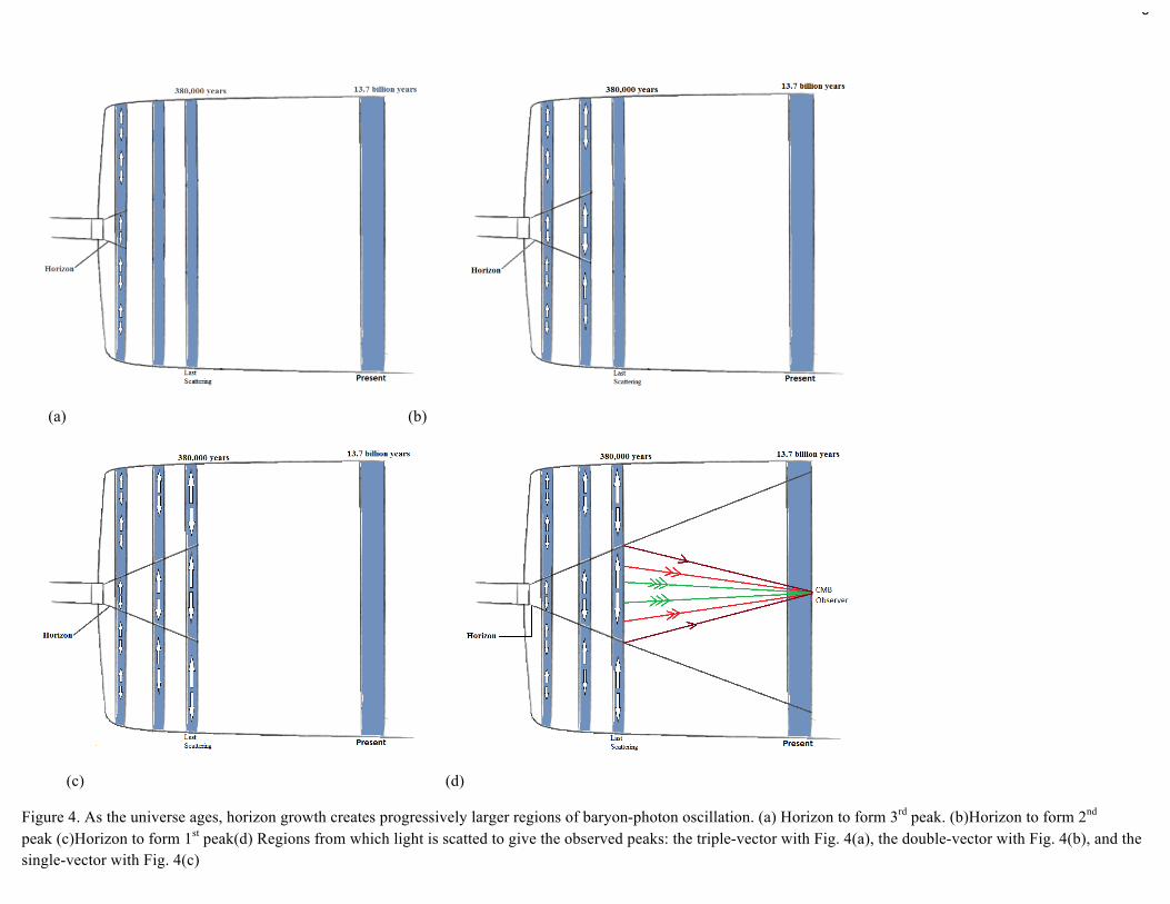
Fig. 2 can be viewed as being on the scale of 89.3Mpc (=291Mly) of today’s universe, from Fig. 3. The pressure exerted on baryons by photons causes expansion, but the dark matter’s gravity tends to keep the baryons compressed. Oscillation of the photons and baryons is reflected in the acoustic peaks of Fig.1, as will be explained below. Power Spectrum Physics The horizon is the farthest distance over which acoustic waves, analogous to sound waves, have had a chance to travel during a certain time. The first peak in the power spectrum of Fig.1 is the result of compression over the farthest distance, i.e. 380,000 years of sound travel. Other peaks in the power spectrum are due to expansion (for even numbered peaks) and compression (for odd numbered peaks) over distances less than 380,000 years of sound travel. Now consider the chronology for formation of the peaks. Third Peak. Baryons are compressed within a comparatively small horizon (see Fig. 4(a)) at an early time in the universe. Then photons cause the baryons to expand, and afterwards they compress again due  to the gravity of dark matter, as illustrated in Fig. 2. The arrows in Fig. 4(a) indicate oscillating baryons and photons. At the instant of the last baryon compression, 380,000 after the Big Bang, light scatters from the compression region (triple-vector lines in Fig. 4(d)) to form the third peak of Fig. 1, and atoms become neutral so the scattered light reaches us with limited re-scattering.

Second Peak. Baryons are compressed within the growing horizon, (see Fig. 4(b)) comparatively larger than the horizon in Fig. 4(a). The photons cause the baryons to expand, against the gravitational force of dark matter as illustrated in Fig. 2. The arrows in Fig. 4(b) indicate oscillating baryons and photons. At the instant of last baryon expansion, 380,000 years after Big Bang, light scatters from the expanded region (double-vector lines in Fig. 4(d)), to form the second peak of Fig. 1, as atoms become neutral so the scattered light reaches us with limited re-scattering.

First Peak. Baryons are compressed within a comparatively larger, growing horizon (see Fig. 4(c)). The gravity of dark matter causes baryons to compress, as illustrated in Fig. 2. This is the largest scale of compression. At the instant of this compression, 380,000 years after Big Bang, light scatters from the

4    

compressed region (single-vector lines in Fig. 4(d)) to form the first peak of Fig. 1 and, like before, atoms become neutral so the scattered light reaches us with limited re-scattering.

(a) (b)

(c)

Figure 2. Oscillating charged baryons (protons) and photons. (a) Baryons attracted by gravitational force of dark matter. (b) Baryons being compressed due to the gravitational force of dark matter. (c) Baryons rebounding due to the photon pressure, pushing the baryons away from dark matter.

5    

Figure 3. Simulation of the universe after 13.6Gyr from the Millennium Simulation Project. Scale is 125Mpc/h=179Mpc=582Mly (http://www.mpa-garching.mpg.de/galform/virgo/millennium/)

All peaks, first, second and third, are formed at the same time; the figures clarify the meaning of horizon and the scale of fluctuation of baryons and photons for different peaks. From Fig. 4(d), we see that all the light waves arrive at the CMB observer at the same time. Fig. 5 shows the different horizon sizes and oscillation of baryons and photons. There are three different sized ellipses in the diagram. The largest ellipse represents the largest horizon from which light scatters to form the first peak. Similarly the second largest ellipse and the smallest ellipse represent horizons from which light scatters to give the second and third peaks. Of course the oscillations do not occur horizontally or vertically; the oscillations occur in random orientations. Figure 5 is just a crude representation of the real universe.

6    

(a) (b)

(c) (d)

Figure 4. As the universe ages, horizon growth creates progressively larger regions of baryon-photon oscillation. (a) Horizon to form 3rd peak. (b)Horizon to form 2nd peak (c)Horizon to form 1st peak(d) Regions from which light is scatted to give the observed peaks: the triple-vector with Fig. 4(a), the double-vector with Fig. 4(b), and the single-vector with Fig. 4(c)

7    

Figure 5. Schematic of the horizon sizes to form the first, second, and third peaks of the power spectrum (Fig.1) 380,000 years after the Big Bang. Different sized ellipses represent different horizon sizes. The arrows represent the oscillation of baryons and photons.

There are other smaller peaks to the right of the power spectrum, but they will not be considered. The CMB power spectrum is a more complex phenomenon than is explored in this lab, much more than sound fluctuation, compression and expansion.

First we are going to change the value of Ωb to see how it affects the power spectrum, and age of universe.

Predictions for Baryon Density Changes

• By considering Figure 2, what change in height do you expect to see in the first peak while increasing Ωb, the baryon density fraction? Why?

__________________________________________________________________________________________________________________________________________________________________________

• By considering Figure 2, what change in height do you expect to see in the second peak while

increasing Ωb? Why? __________________________________________________________________________________________________________________________________________________________________________

8    

Directions for Exploring Baryon Density Changes

1. Go to the CAMB Web Interface at the website http://lambda.gsfc.nasa.gov/toolbox/tb_camb_form.cfm to generate the theoretical temperature maps and power spectra. Choose “Sky Map Output: Temperature Only,” “Beam Size (arcmin) 13.5,” and “Synfast Random # Seed 2735.” (The Seed insures that the random number generator starts at the same value every time, important for making comparisons, so a value can be set other than 2735, but that value must be used throughout the lab.) You will explore what happens as a result of changing Ωb, the fractional baryon density. We will first obtain the power spectrum for a flat universe. To do so, set Ωk= 0, then press “Go!” at the bottom of the page.

2. After a while, a page of “Output from CAMB” will be returned. Find the value Om_b h^2, then calculate Ωb = (Om_b h^2)/(0.7)2 and record it in the table below. Also record Age of universe, Om_K, Om_Lambda, and Om_m.

3. From the output page, download a file that has a name similar to camb_67260122_scalcls.dat. Be sure to include the label k0 in the saved file name.

4. Refresh the CAMB Web Interface page, and again set “Sky Map Output: Temperature Only,” “Beam Size (arcmin) 13.5,” and “Synfast Random # Seed 2735,” but set the option “Use Physical Parameters” to “No.”

5. A list of boxes comes up to the right of Cosmological Parameters: change Ωb to 0.03, record this in the table below, then press “Go!”. Be sure that the seed value is the same as before.

6. From the “Output from CAMB” page, record Age of universe, Om_K, Om_Lambda, and Om_m. 7. Download the scalcls.dat file, being sure to include b03 in the file name. 8. Repeat steps 3, 4, and 5 but with a value of Ωb = 0.07. 9. Import the data from the three scalcls.dat files into a spreadsheet by first importing the b03 file,

then deleting all but the first two columns. Then import the k0 and b07 files, but keep only the second columns from those files. Insert a row at the top for the labels: l, Ωb = 0.03, Ωb = your table value, and Ωb = 0.07.

10. Make “Smooth Lined Scatter” graphs (power spectra) of the three columns, all on the same plot, then record the peak heights. Recall that the power spectra represent temperature fluctuations.

Ωb Age of Universe (Gyr)

First peak height

Second peak height

Third peak height

Ωk ΩΛ Ωm

• How does the height of the first peak change as baryon density increases? _______________________________________________________________________________________________________________________________________________________________________________________________________________________________________________________________

9    

• How does the height of the second peak change as baryon density increases? __________________________________________________________________________________________________________________________________________________________________________________________________________________________________________________

• Do your observations match your predictions? _________________________________________________________________________________ _________________________________________________________________________________

• As baryon density increases, how does the angular scale of first peak change? __________________________________________________________________________________________________________________________________________________________________________________________________________________________________________________ • How does increasing baryon density affect the age of the universe? ___________________________________________________________________________________________________________________________________________________________________________________________________________________________________________________

• Do your predictions about the 1st and 2nd peaks match the above observations? If not consult your

instructor. ___________________________________________________________________________________________________________________________________________________________________________________________________________________________________________________

Now we will work on the density of dark matter and how it affects the power spectrum as well as the age of the universe.

Predictions for Dark Matter Density Changes

• By considering Figure 2, what change in height do you expect in the first peak as the dark matter density fraction, Ωcdm, is increased? Why?

___________________________________________________________________________________________________________________________________________________________________________________________________________________________________________________

• By considering Figure 2, what change in angular size of a fluctuation region (l-value) do you

expect in the first peak as Ωcdm is increased? Why? ___________________________________________________________________________________________________________________________________________________________________________________________________________________________________________________

10    

Directions for Exploring Dark Matter Density Changes

1. Refresh the CAMB Web Interface page, and set “Sky Map Output: Temperature Only,” “Beam Size (arcmin) 13.5,” and “Synfast Random # Seed 2735,” but set the option “Use Physical Parameters” to “No.”

2. A list of boxes comes up to the right of Cosmological Parameters. Set the dark matter, dark energy and baryon parameters to Ωcdm = 0.15, ΩΛ = 0.72, and Ωb = 0.046, record in the table below, then press “Go!”. Be sure that the seed value is the same as before.

3. From the “Output from CAMB” page, record the Age of Universe, and Om_K below. 4. Download and save the scalcls.dat file, being sure to include cdm15 in the file name. 5. Repeat steps 1-4, but with the change Ωcdm = 0.234. 6. Repeat steps 1-4, but with the change Ωcdm = 0.4. 7. Import the data from the three scalcls.dat files into a spreadsheet by first importing the cdm15

file, then deleting all but the first two columns. Then import the cdm234 and cdm4 files, but keep only the second columns from those files. Insert a row at the top for the labels: l, Ωcdm = 0.15, Ωcdm = 0.234, and Ωcdm = 0.4.

8. Make “Smooth Lined Scatter” graphs (power spectra) of the three columns, all on the same plot, then record the peak heights.

Ωcdm Age of Universe (Gyr)

First peak height

Second peak height

Third peak height

Ωk ΩΛ Ωb

• How does the height of the first peak change as the dark matter density increases? ___________________________________________________________________________________________________________________________________________________________________________________________________________________________________________________ • Considering only the first peak, how does the angular size of a fluctuation region (l-value) change

as dark matter density increases? ___________________________________________________________________________________________________________________________________________________________________________________________________________________________________________________

• Do your predictions match the data in the table? If not consult your professor.

___________________________________________________________________________________________________________________________________________________________________________________________________________________________________________________

11    

• How does increasing the dark matter density affect the age of universe? ___________________________________________________________________________________________________________________________________________________________________________________________________________________________________________________

Predictions for Dark Energy Density Changes

• By considering that dark energy acts as anti-gravity, what change in angular size of a fluctuation region (l-value) do you expect in the first peak as the dark energy density fraction, ΩΛ, is increased? Why?

__________________________________________________________________________________________________________________________________________________________________________

Directions for Exploring Dark Energy Density Changes 1. Refresh the CAMB Web Interface page, and set “Sky Map Output: Temperature Only,”

“Beam Size (arcmin) 13.5,” and “Synfast Random # Seed 2735,” but set the option “Use Physical Parameters” to “No.”

2. A list of boxes comes up to the right of Cosmological Parameters. Set Ωcdm = 0.234, ΩΛ = 0.6, and Ωb = 0.046, record in the table below, then press “Go!”. Be sure that the seed value is the same as before.

3. From the “Output from CAMB” page, record the Age of Universe, and Om_K below. 4. Download and save the scalcls.dat file, being sure to include L6 in the file name. 5. Repeat steps 1-4, but with the change ΩΛ = 0.72. 6. Repeat steps 1-4, but with the change ΩΛ = 0.8. 7. Import the data from the three scalcls.dat files into a spreadsheet by first importing the L6

file, then deleting all but the first two columns. Then import the L72 and L8 files, but keep only the second columns from those files. Insert a row at the top for the labels: l, lambda=0.6, lambda=0.72, and lambda=0.8.

8. Make “Smooth Lined Scatter” graphs (power spectra) of the three columns, all on the same plot, then record the peak heights.

ΩΛ Age of Universe (Gyr)

First peak height

Second peak height

Third peak height

Ωk Ωcdm Ωb

• How does the angular size of a fluctuation region (l-value) represented by the first peak change as the dark energy density fraction, ΩΛ, is increased?

___________________________________________________________________________________________________________________________________________________________________________________________________________________________________________________

12    

• Is your finding for the 1st peak also true for the 2nd peak? ___________________________________________________________________________________________________________________________________________________________________________________________________________________________________________________ • How does the height of the first peak change as the dark energy density increases? ___________________________________________________________________________________________________________________________________________________________________________________________________________________________________________________ • How does increasing the dark energy density affect the age of universe? ___________________________________________________________________________________________________________________________________________________________________________________________________________________________________________________

Copyright © 2015 by Daniel M. Smith, Jr.

References

Duncan, T. and Tyler, C., 2009, Your Cosmic Context (San Francisco, California)