clustering on graphs: the markov cluster algorithm...

Clustering on Graphs:

The Markov Cluster Algorithm

(MCL)

CS 595D Presentation

By Kathy Macropol

MCL Algorithm

� Based on the PhD thesis by Stijn van Dongen

Van Dongen, S. (2000) Graph Clustering by Flow

Simulation. PhD Thesis, University of Utrecht, The

Netherlands.

� MCL is a graph clustering algorithm.

� MCL is freely available for download at

http://www.micans.org/mcl/

Outline

� Background

– Clustering

– Random Walks

– Markov Chains

� MCL

– Basis

– Inflation Operator

– Algorithm

– Convergence

� MCL Analysis

– Comparison to Other Graph Clustering Algorithms

• RNSC, SPC, MCODE

• RRW

� Conclusions

Graph Clustering

� Clustering – finding natural groupings of items.

� Vector Clustering Graph Clustering

Each point has

a vector, i.e.

• x coordinate

• y coordinate

• color

1

3

4

4

4

34

34

2

3

Each vertex is

connected to

others by

(weighted or

unweighted)

edges.

Random Walks

� Considering a graph, there will be many links within a cluster, and fewer links between clusters.

� This means if you were to start at a node, and then randomly travel to a connected node, you’re more

likely to stay within a cluster than travel between.

� This is what MCL (and several other clustering algorithms) is based on.

– Other ways to consider graph clustering may include, for example, looking for cliques. This tends to be sensitive to changes in node degree, however.

Random Walks

� By doing random walks upon the graph, it may be possible to discover where the flow tends to gather,

and therefore, where clusters are.

� Random Walks on a graph are calculated using

“Markov Chains”.

Markov Chains� To see how this works, an example:

� In one time step, a random walker at node 1 has a 33% chance of going to node 2, 3, & 4, and 0% chance to nodes 5, 6, or 7.

� From node 2, 25% chance for 1, 3, 4, 5 and 0% for 6 and 7.

� Creating a transition matrix gives:

1 2

3 45

6

7

0 .25 .33 .33 0 0 0

.33 0 .33 .33 .33 0 0

.33 .25 0 .33 0 0 0

.33 .25 .33 0 0 0 0

0 .25 0 0 0 .5 .5

0 0 0 0 .33 0 .5

0 0 0 0 .33 .5 0

1

2

3

4

5

6

7

1 2 3 4 5 6 7

Also can be looked at as a probability matrix!

(notice each

column sums

to one)

Markov Chains

� A simpler example:

� Next time step:

.6 .2

.4 .8

.6 .2

.4 .8

.6 .2

.4 .8=

t0 t1 t2

1 1 1 + 1 2 1

.6 * .6 + .4 * .2 = .44

.44 .28

.56 .72

.33 .33

.66 .66

eventually

.35 .32

.65 .68

.34 .33

.66 .66

Markov Chain

� Markov Chain: A sequence of variables X1, X2, X3, etc (in our

case, the probability matrices) where, given the

present state, the past and future states areindependent.

� Probabilities for the next time step only depend on current probabilities (given the current probability).

� A random walk is an example of a Markov Chain, using the transition probability matrices.

Weighted Graphs

� To turn a weighted graph into a probability (transition) matrix,

column normalize.

1 2

3 4

2

231

0 2 1 3

2 0 0 2

1 0 0 0

3 2 0 0

0 1/2 1 3/5

1/3 0 0 2/5

1/6 0 0 0

1/2 1/2 0 0

Notice it’s no longer

symmetric.

Adding Self Loops

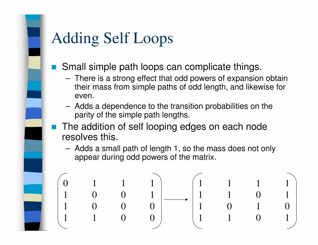
� Small simple path loops can complicate things.– There is a strong effect that odd powers of expansion obtain

their mass from simple paths of odd length, and likewise for even.

– Adds a dependence to the transition probabilities on the parity of the simple path lengths.

� The addition of self looping edges on each node resolves this.– Adds a small path of length 1, so the mass does not only

appear during odd powers of the matrix.

0 1 1 1

1 0 0 1

1 0 0 0

1 1 0 0

1 1 1 1

1 1 0 1

1 0 1 0

1 1 0 1

Markov Chain Cluster Structure

� Example:

0 .25 .33 .33 0 0 0

.33 0 .33 .33 .33 0 0

.33 .25 0 .33 0 0 0

.33 .25 .33 0 0 0 0

0 .25 0 0 0 .5 .5

0 0 0 0 .33 0 .5

0 0 0 0 .33 .5 0

.15 .15 .15 .15 .15 .15 .15

.2 .2 .2 .2 .2 .2 .2

.15 .15 .15 .15 .15 .15 .15

.15 .15 .15 .15 .15 .15 .15

.15 .15 .15 .15 .15 .15 .15

.1 .1 .1 .1 .1 .1 .1

.1 .1 .1 .1 .1 .1 .1

eventually

Notice that, in the beginning time steps, before the flow really mixes, the

cluster structure is pronounced in the matrix!

This is not a coincidence, and MCL uses this, modifying the random walk

process to further emphasize the divide between clusters in the matrix.

1 2

3 45

6

7

MCL

� "Flow is easier within dense regions than across sparse boundaries, however, in the long run this

effect disappears."

� During the earlier powers of the Markov Chain, the

edge weights will be higher in links that are within

clusters, and lower between the clusters.

� This means there is a correspondence between the

distribution of weight over the columns and theclusterings.

MCL

� MCL deliberately boosts this affect by

– Stopping partway in the Markov Chain

– Then adjusting the transitions by columns.For each vertex, the transition values are changed so that

• Strong neighbors are further strengthened

• Less popular neighbors are demoted.

� This adjusting can be done by raising a single column to a non-negative power, and then re-normalizing.

� This operation is named “Inflation”

� (Taking the Markov Chain powers is named

“Expansion”)

MCL Inflation

� Example for inflation of 2 (squaring):

Square, and

then normalize

MCL Inflation

MCL Inflation

� The inflation operator is responsible for both strengthening and weakening of current.

(Strengthens strong currents, and weakens already

weak currents).

� The inflation parameter, r, controls the extent of this

strengthening / weakening. (In the end, this influences the granularity of clusters.)

MCL Algorithm

� In MCL, the following two processes are alternated between repeatedly:

– Expansion (taking the Markov Chain transition matrix powers)

– Inflation

� The expansion operator is responsible for allowing

flow to connect different regions of the graph.

� The inflation operator is responsible for both

strengthening and weakening of current.

MCL Algorithm

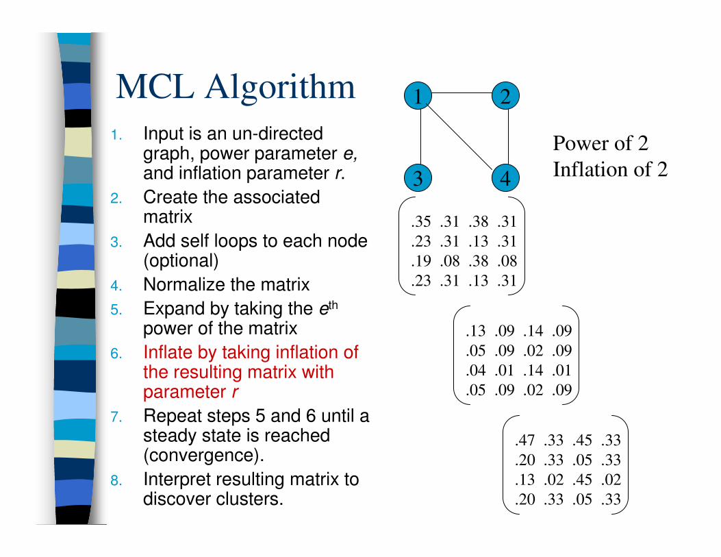
1. Input is an un-directed graph, power parameter e,

and inflation parameter r.

2. Create the associated matrix

3. Add self loops to each node (optional)

4. Normalize the matrix

5. Expand by taking the eth power of the matrix

6. Inflate by taking inflation of the resulting matrix with parameter r

7. Repeat steps 5 and 6 until a steady state is reached

(convergence).

8. Interpret resulting matrix to discover clusters.

MCL Algorithm

1. Input is an un-directed graph, power parameter e,and inflation parameter r.




5. Expand by taking the eth

power of the matrix


7. Repeat steps 5 and 6 until a steady state is reached (convergence).


1 2

3 4

Power of 2

Inflation of 2

MCL Algorithm






power of the matrix




1 2

3 4

Power of 2

Inflation of 2

0 1 1 1

1 0 0 1

1 0 0 0

1 1 0 0

MCL Algorithm






power of the matrix




1 2

3 4

Power of 2

Inflation of 2

0 1 1 1

1 0 0 1

1 0 0 0

1 1 0 0

1 1 1 1

1 1 0 1

1 0 1 0

1 1 0 1

MCL Algorithm






power of the matrix




1 2

3 4

Power of 2

Inflation of 2

1 1 1 1

1 1 0 1

1 0 1 0

1 1 0 1

1/4 1/3 1/2 1/3

1/4 1/3 0 1/3

1/4 0 1/2 0

1/4 1/3 0 1/3

MCL Algorithm






power of the matrix




1 2

3 4

Power of 2

Inflation of 2

¼ 1/3 ½ 1/3

¼ 1/3 0 1/3

¼ 0 ½ 0

¼ 1/3 0 1/3

¼ 1/3 ½ 1/3

¼ 1/3 0 1/3

¼ 0 ½ 0

¼ 1/3 0 1/3

=

.35 .31 .38 .31

.23 .31 .13 .31

.19 .08 .38 .08

.23 .31 .13 .31

MCL Algorithm






power of the matrix




1 2

3 4

Power of 2

Inflation of 2

.35 .31 .38 .31

.23 .31 .13 .31

.19 .08 .38 .08

.23 .31 .13 .31

.13 .09 .14 .09

.05 .09 .02 .09

.04 .01 .14 .01

.05 .09 .02 .09

.47 .33 .45 .33

.20 .33 .05 .33

.13 .02 .45 .02

.20 .33 .05 .33

MCL Algorithm






power of the matrix




1 2

3 4

Power of 2

Inflation of 2

.94 .33 .50 .33

.03 .33 -- .33

.01 -- .50 --

.13 .33 -- .33

.70 .33 .49 .33

.12 .33 .01 .33

.05 .02 .49 --

.12 .33 .01 .33

1 .33 .50 .33

-- .33 -- .33

-- -- .50 --

-- .33 -- .33

MCL Algorithm






power of the matrix




1 2

3 4

Power of 2

Inflation of 2

Expand on in

just a minute.

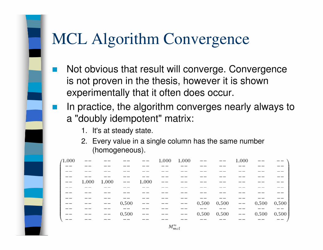
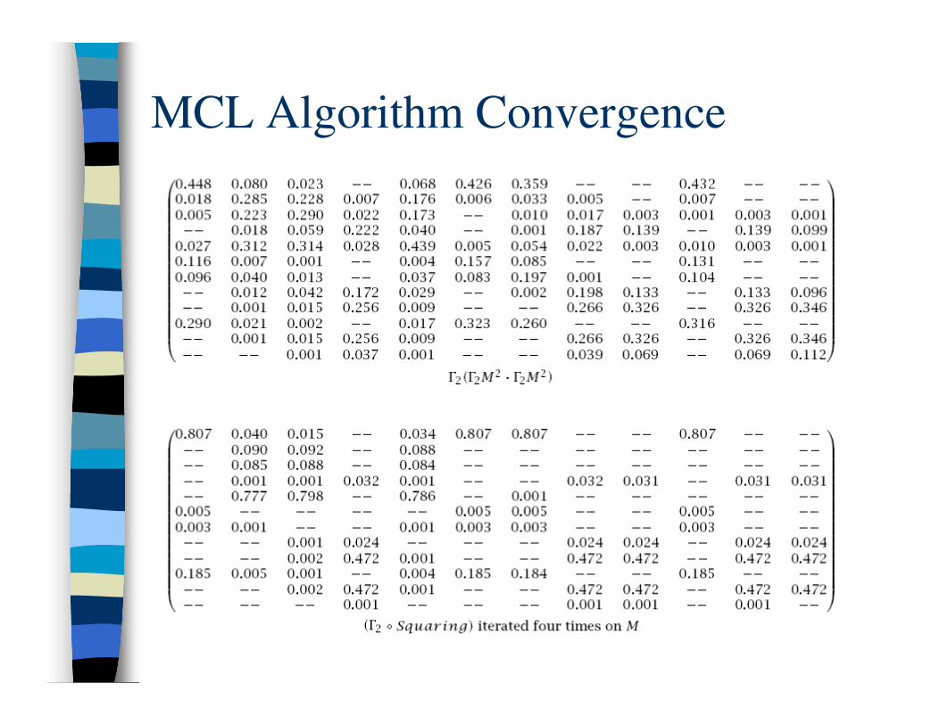
MCL Algorithm Convergence

� Not obvious that result will converge. Convergence is not proven in the thesis, however it is shown

experimentally that it often does occur.

� In practice, the algorithm converges nearly always to

a "doubly idempotent" matrix: 1. It's at steady state.

2. Every value in a single column has the same number

(homogeneous).


� It is proven that when the matrix is in the neighborhood of being doubly idempotent, it converges quadratically.

� However, the final steady state may sometimes be cyclic and consist of a repeating series of matrices.– In certain cases, the expansion and inflation act as inverses

of each other. However, a slight change of parameters and the equilibrium is broken.

– Without self loops, it’s possible on bipartite graphs because of odd path lengths. Adding self loops and slightly changing parameters fixes most of the problems.

– Other graphs that may have periodic behavior are described, but will most likely be "a curiosity lacking cluster structure anyhow".


MCL Animated

MCL Interpreting Clusters

� To interpret clusters, the vertices are split into two types. Attractors, which attract other vertices, and

vertices that are being attracted by the attractors.

� Attractors have at least one positive flow value within

their corresponding row (in the steady state matrix).

� Each attractor is attracting the vertices which have positive values within its row.


� Attractors and the elements they attract are swept together into the same cluster.

� In this case, {1, 6, 7, 10}, {2, 3, 5}, {4, 8, 9, 11, 12}


� In general, overlapping clusters (where one node is contained in multiple clusters) are only found in very

special cases of graph symmetry:

– Only when a vertex is attracted exactly equally by more than one cluster

– This occurs only when both clusters are isomorphic

1 2 3 4 5 6 7

MCL Clusters

� The inflation parameter affects cluster granularity(a is the weight for added self loops)

MCL Clusters

� For clusters with large diameter, MCL has problems

� Distributing flow across cluster needs long expansion and low inflation (otherwise the cluster will split).

� Takes many iterations and causes MCL to be sensitive to small perturbations in the graph.

– The addition of small diameter clusters disturbs the clustering, since the low inflation parameter will cause them to disproportionately ‘inflate’ surrounding probabilities.

Analysis of MCL

� O(N3), where N is the number of vertices.

– N3 cost of one matrix multiplication on two matrices of dimension N.

– Inflation can be done in O(N2) time

– The number of steps to converge is not proven, but experimentally shown to be ~10 to 100 steps, and mostly consist of sparse matrices after the first few steps.

� Speed may be improved through pruning.

– Inspect matrix and set small values directly to zero (assume they would have reached there eventually anyways).

– Works well when the diameter of the clusters is small. (Non-homogeneous distributions of weight)

Analysis of MCL

� In 2006, MCL fared well in a paper comparing it to three other clustering techniques

– Brohee S, van Helden J (2006) Evaluation of clustering algorithms for protein–protein interaction networks. BMC Bioinformatics 7: 488

– MCL vs. Restricted Neighborhood Search Clustering (RNSC) vs. Super Paramagnetic Clustering (SPC) vs. Molecular Complex Detection (MCODE)

Analysis of MCLEach curve represents the value

of accuracy (left panels) or

separation (right panels).

(A-B) edge addition to the test

graph. (C-D) edges removal

from the test graph. (E-F) Edge

removal from an altered graph

with 100% of randomly added

edges. (G-H) Edge addition to

an altered test graph with 40%

of randomly removed edges.

Color code: blue : MCL, red :

RNSC, orange : MCODE,

green : SPC. Dotted lines show

the results obtained by

permuting the clusters (negative

control).

MCL Compared to RRW

� Comparison to Repeated Random Walks (RRW)

– RRW is another Graph Clustering Method.

• Every cluster (including intermediate clusters) is stored.

• Clusters that overlap more than a threshold are later

compared, and lower ranking clusters removed.

MCL Compared to RRW

� RRW Cluster p-value approximation:

where n is the number of vertices in the cluster, and score is the average random walk distance between

nodes in the cluster.

.1

.3

.3.3

.1.1

(.1+.3+.1+.1+.3+.3)

score = 6 = .2

p-value = 1 – (.2 * √ 3 ) = 0.653

MCL Compared to RRW

� MCL, RRW, and a naïve nearest neighbor approach were run on a biological protein network for yeast (WI-PHI1), as well as “noisy” versions of the network (edges added and deleted).

� Proteins with the same biological function should be clustered together

� The resulting clusters were compared to known protein groupings.

1Kiemer L, Costa S, Ueffing M, Cesareni G: WI-PHI: A weighted yeastinteractome enriched for direct physical interactions. Proteomics 2007, 7:932–943.

MCL Compared to RRW

Average cluster size: RRW = 6, MCL = 12, Naïve = 9

Analysis of MCL

� Scales well with increasing graph size.

� Works with both weighted and unweighted graphs.

� Produces good clustering results.

� Robust against noise in graph data

� Number of clusters not specified ahead of time, but

can adjust cluster granularity with parameters.

� Cannot find overlapping clusters (in general)

� Not suitable for clusters with large diameter.

Thank You!

Any Questions?

clustering on graphs: the markov cluster algorithm...

Documents