Clustering: “global” indexes (to measure the ‘global’degree of clustering for the whole set of events) -> methodsbased on quadrats (joint count) vs. on distances

AVERAGE NEAREST NEIGHBOUR: the distance betweenevents is less (clustering) or more (pattern inibitorio) of the expected distance in case of complete spatial randomness? (Clark-Evans, ’50s)

Nearest neighbour ratio = observed mean distance / expectedmean distance (CSR) ->

Input:Points: unweighted (= 1) / Projected coordinate system!(Polygons and lines: convert into points with x, y = centroids)

Output:- Observed Mean Distance-Expected Mean Distance- Nearest Neighbor Index-Graphic report- Test variables:p-value: probabilty of the spatial distribution to be random

z-score: standard deviation of the real values from expected values

- measure the ANN for firms within the GRA (selection ofrm_immig.shp)

-> Toolbox / Spatialstatistics / Analyzingpatterns

Bivariate point patterns : co-agglomeration, co-location, competition/cooperation, related variety: Bivariate/Cross K function, Pairwise interaction point process.. Crimestat, R..

Multi-variate point patterns… (…). -> Bivariate pointpatterns analysis for each couple of patterns

Risk-Adjusted Nearest Neighbor Hierarchical SpatialClustering (Rnnh) (Crimestat)Clustering index in which the probability of identifying clustersfor certain categories of events is assessed in relation to the spatial distribution of all events, by using an interpolationbetween the (kernel) density surfaces of the primary file (e.g. crimes) and the secondary files (eg. population)

Clustering processes at different scales

In the figure: 10 clusters of first order, 8 clusters ofsecond order, 3 of third order, and so on..

NEAREST NEIGHBOR HIERARCHICAL CLUSTER: constant-distance clustering routine for non-weighted events, hierarchical: first orderclusters are consideredpoints which may cluster at the second order and so on, until criteria are satisfied(for each order).

Output (dbf, shp): n. cluster, mean center, deviational ellipseand convex hull (spezzata) of points beloning to each cluster, area and cluster density.Results are heavily influenced by the identified first order clusters

RIPLEY'S K-FUNCTION: To identifyclustered/inhibitory/random point patterns t differentscales/distances between points (Ripley 1976, 1981 “Spatialstatistics”)

Two uses: to confirm/reject the null/random hypothesis at various scales/distances + to dientify the scale/distancewhere the clustering/inhibition is more intense/weak

K = expected number of events / real number of events

In case of complete spatial randomness: K(d) = πd2 :

Linearization of the K function: L function (Besag 1977)

In case of complete spatial randomness: L(d) = d (ArcGIS):

Or L(d) = 0 ->

(Crimestat)

K value (clustering)

Confidence interval

Expected value

Confidence interval

Ripley’s K

Lower and upper confidence envelops: beyond whichresults may be considered significant

Confidence envelops are estimated thanks to the reiterationof a Montecarlo simulation (Crimestat: 100 simulations; ArcGIS: 0 / 9%, 99% o 99,9% of the confidence interval). Corollary: simulations work better if the number of points isnot small (> 100)

Maximum distance

Crimestat: SQRT(A)/3

ArcGIS: ?

Distance ranges

Crimestat: 100

ArcGIS: from 1 to 100 (or: “beginning distance” + “distance increment”)

Spatial statistics / Analyzing patterns / Multi-Distance Spatial Cluster Analysis

(K function) other parameters:

Weight field: default: 1, fixed: weight (number of eventsat each point). The weighted estimation gives differentresults (clustering is likely to be higher)

!: points cannot have distance=0*

Is an “area sensitive” tool: results are influenced by the area extension

Study area methods:

Default: minimum enclosing rectangle

User provided: via polygonial layer -> «Study Area»

Problems with the analysis of spatial data #1:

-Study area extension (if too small, the analysis may notinclude elements which are important to provide anexhaustive explanation. If too big, the spatial distributionpattern may be due of a diversity of processes which havenothing to do with what we want to explain. Example: suburban, scattered and low density urban areas).

-> reduce the size of the area

Creat a mask of the area within the GRA (ring road) by selecting (manually) the zone urbanistiche within the GRA and exporting the selection as mask_area.shp

Specific problems in the analysis of spatial data #2: Boundary problems: given the probability of non observedevents beyond the study area’s boundaries (with a similar or dissimilar spatial distribution), con distribuzione spaziale simile o dissimile), clustering near the boundaries is under-estimated.

Boundary correction methods:NONE: because events are only to be found within the boundaries. Or because the point layer is wider than the study area: pointsbeyond the boundaries of the study area are used for estimatingthe K function (!!!)SIMULATE_OUTER_BOUNDARY_VALUES: simulate a «mirrored»distribution of points beyond the bounadriesREDUCE_ANALYSIS_AREA: reduces the study area.RIPLEY'S_EDGE_CORRECTION_FORMULA: those points whosedistance from the boundary is smaller than to other points, are weighted more (good only for non irregular study areas)

Output: table(+ Display result graphically): - ExpK (K expected value in case of CSR), - Envelopes (confidence intervals), - ObservedK (value of K)- DiffK (ObservedK-ExpK)

Cautions:- Works better for clustered than for inhibitory processes- It’s mainly a tool for identifying second-order clusters, i.e. localized clusters, intra-regional scales or medium distances. - Not reliable for small numbers of events (>30, >100)- Not reliable for strongly irregular areas (if it’s not possibleto solve adequately the boundary problem)

Measure the Ripley K function for the distribution of firmsowned by foreigners within the GRA (ring road)

Input: vv/rm_immig_wdata.shp(Confidence envelop: 0 permutations)*Click “Display results graphically”Distance bands: 20Weight field: “CNT”Beginning distance: 250Distance increments: 250Boundary correction method: NONE, because:Study area: “User provided” = dropbox/corsi-memotef/lezgis16/4/mask.shp

Verify the graphic and table (diff) output

Space-timeRipley’s K

Global indexes of spatialautocorrelation

Taxonomy of spatial analysis tools (in ArcGIS and Crimestat)

Of events (spatial distribution) Of intensities (spatialassociation)

Global indexes

Average nearest neighbour

(Multi‐scale) K‐Ripley

Global indexes ofautocorrelation: 

Moran’s I

Geary’s C

Localindexes

Kernel density maps

Nearest neighbour hierarchicalclustering

Risk‐Adjusted Nearest Neighbor Hierarchical Clustering

Local indicators of spatialassociation (LISA): 

Local Anselin of Moran’s I (Cluster and outlier analys.)

Getis‐Ord Gi (Hot‐spotanalysis)

3. Global indexes of spatial AUTOCORRELATION

First law of geography (Tobler) = "Everything is related to everything else, but near things are more related than distant things."

It’s a form of spatial dependence (positive or negative): the degree to which nearby features are similar or dissimilar*, vs. an hypothesis of complete spatial randomness.

- Similar to time series analysis, but both proximity AND direction/position (2D)

Why to estimate the degree of spatial autocorrelation:

- To understand the process (or the variety of processes..) which explain the geographical distribution of intensities

- To estimate the degree to which nearby features potentiallyinfluence each other (=interaction, interdependence, attraction, contagion, clustering, segregation, etc…)

- To verify the degree to which the observed variables are (not) statistically indipendent (eg. autocorrelation reducesthe dataset’s information content or obscures what is specificabout each area, because intensities in one area are partiallyinfluenced by what is happening nearby)

- (Eg. to test the spatial autocorrelation of models’ residuals)

- (Eg. to assist in the identification of the spatial sample size)

Exploratory Spatial Data Analysis (and mapping) vs. Modelling (formal verification and testing of hypothesis)

Spatial auto-correlation: global indexes

Spatial autocorrelation (MORAN’S I):

Global co-variance index adapted from the analysis ofthe ‘memory’ effect in time series (Moran ’40s, Whittle1954).

Measures the “gobal” degree of similarity between the (upper and lower) intensities (-/+) of nearby features

Moran’s I

Xi – X = intensity in point Xi – average intensity

(Xi-X)(Xj-X): Cross-product, high if values are similar

Wij: spatial weights (/influences) matrix *

Clustered/high autocorrelation if I is high (I>0), dispersed/low autocorrelation if I is low (I<0), vs. the CSR hypothesis Iexp=-[1/(n-1)]

Spatial statistics / Analyzing patterns / Spatial autocorrelation (Moran’s I) Conceptualization of spatial relationships:

Inverse distance (squared): spatial relationshipsbetween features are inversely proportional to their(squared) distance. Computational problems withsmall distances (crimestat: “adjust for smalldistances”) and no threshold (n to n)

Fixed distance band: within the threshold (band) anyfeature weights 1. Appropriate in the case of non-uniformpolygons, and for large point datasets.

Zone of indifference: neighbors (or features withinthe distance threshold) weight 1. Other features’weight is inversely proportional to their distance. Appropriate as above, when the influence of distantfeatures is relevant. Computational problems.

Polygon contiguity (adjacency!): considers only borderingfeatures (1 if bordering, 0 all the others). Appropriate only forregular polygons (original Moran’s I. Generalized by Cliff and Ord1973. Widely used in spatial econometrics)

Conceptualization of spatial relationships (2):

Distance Band or Threshold Distance (mostly for largedatasets): threshold beyond which influence is null (with “inverse distance” = i) 0: all features are considered; ii) Empty: applies a default threshold distance (min distance at which any feature hasa neighbour); iii) defined by the user

Weights Matrix from file: uses a spatial weight matrix file (.swm) created/adapted by the user

Spatial weight matrix

Table in .swm format in which any cell includes anexpression of the distance, time, cost, influence, spatial relationship between any couple of features (presence/absence or intensity)

Spatial statistics / Modeling spatial relationships / Generate spatial weight matrix

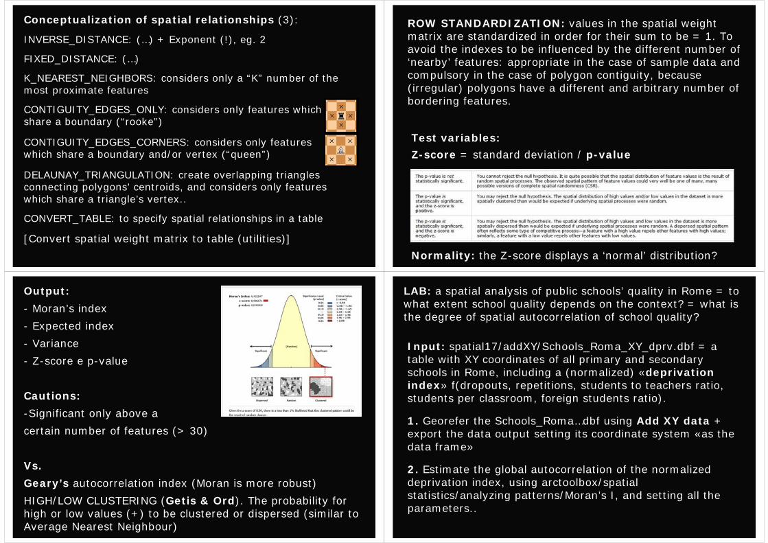
Conceptualization of spatial relationships (3):

INVERSE_DISTANCE: (…) + Exponent (!), eg. 2

FIXED_DISTANCE: (…)

K_NEAREST_NEIGHBORS: considers only a “K” number of the most proximate features

CONTIGUITY_EDGES_ONLY: considers only features whichshare a boundary (“rooke”)

CONTIGUITY_EDGES_CORNERS: considers only featureswhich share a boundary and/or vertex (“queen”)

DELAUNAY_TRIANGULATION: create overlapping trianglesconnecting polygons’ centroids, and considers only featureswhich share a triangle’s vertex..

CONVERT_TABLE: to specify spatial relationships in a table

[Convert spatial weight matrix to table (utilities)]

ROW STANDARDIZATION: values in the spatial weightmatrix are standardized in order for their sum to be = 1. Toavoid the indexes to be influenced by the different number of‘nearby’ features: appropriate in the case of sample data and compulsory in the case of polygon contiguity, because(irregular) polygons have a different and arbitrary number ofbordering features.

Test variables:Z-score = standard deviation / p-value

Normality: the Z-score displays a ‘normal’ distribution?

Output:- Moran’s index- Expected index- Variance- Z-score e p-value

Cautions:-Significant only above a certain number of features (> 30)

Vs.Geary’s autocorrelation index (Moran is more robust)HIGH/LOW CLUSTERING (Getis & Ord). The probability forhigh or low values (+) to be clustered or dispersed (similar toAverage Nearest Neighbour)

LAB: a spatial analysis of public schools’ quality in Rome = towhat extent school quality depends on the context? = what isthe degree of spatial autocorrelation of school quality?

Input: spatial17/addXY/Schools_Roma_XY_dprv.dbf = a table with XY coordinates of all primary and secondaryschools in Rome, including a (normalized) «deprivationindex» f(dropouts, repetitions, students to teachers ratio, students per classroom, foreign students ratio).

1. Georefer the Schools_Roma…dbf using Add XY data + export the data output setting its coordinate system «as the data frame»

2. Estimate the global autocorrelation of the normalizeddeprivation index, using arctoolbox/spatialstatistics/analyzing patterns/Moran’s I, and setting all the parameters..

LAB: what is the degree of spatial autocorrelation of schoolquality?

2. Estimate the global autocorrelation of the normalizeddeprivation index, using the Moran’s I. Parameters:

Input feature class: schools

Input field = «DPRV_NORM»

Conceptualization of spatial relationships: ?

Row standardization: ?

Threshold distance: 10.000 meters

Generate report

-> Verify the graphic report and test variables: what is the result? Is this statistically significant?

Do high or low quality schools cluster in certain zones, and where? -> Local indicators of spatial autocorrelation…

Local indexes of spatialassociation/autocorrelation

4. LOCAL INDEX OF SPATIAL AUTOCORRELATION

To measure the degree of autocorrelation for eachgeographical feature (where and which features ?)

Anselin local of Moran’s I (Anselin L. 1995, Local indicators ofspatial association – LISA. Geographical Analysis 27, 93-115)

To attribute to each feature a degree of high/low autocorrelation based on its (high/low) intensity beingsimilar/dissimilar to nearby features

Z: intensity, S: variance, W: spatial weight matrix

Input: polygons (crimestat) and points(ArcGIS)

Output:

Cluster type (COType) identifies (and renders):- Features which are part of high (HH) or low (LL) valuesclusters, because nearby features have similar values, and are statistical significant (positive and high z-score).- “outlier” features, with high or low values, surrounded byfeatures with low (HL) or high (LH) values, and are statisticalsignificant (low and negative z-score)

Grado di segregazione tra aree a prevalenza di imprenditori cinesi e aree a prevalenza di imprenditori italiani 

  

Contributo locale alla segregazione tra aree a prevalente presenza di unità condotte da imprenditori cinesi o italiani 

   

Anselin local of Moran’s I of the distance ofentrepreneurs from their country of origin

Spatial statistics / Mapping clusters / Cluster and outlier analysis LAB: a spatial analysis of public schools’ quality in Rome = To what extent school quality depends on the context? Do high or low quality schools cluster in certain zones, and where?

1. Identify and render those schools which are part of clustersof nearby low or high quality schools using arctoolbox/spatialstatistics/mapping clusters/cluster and outlier analysisInput: Schools with data shapefile, input field: DPRV_NORMSpatial relationships: Inverse distance

-> Modify the symbology of the ouput layer in order tovisualize only the schools in clusters of high or low and significant spatial autocorrelation values-> Open and verify the ouput layer attribute table-> In a copied layer, represent the value of the index(L_Milndex) disregarding of the degree of significance- > Check (and try to make sense) of outliers

Local indexes of spatial autocorrelation (2):

Getis-Ord Gi, high/low clustering (Hot Spot Analysis)

Identifies features which are part of “hot spots”: areas withunusual clustering of high or low values (Cliff & Ord, Spatialautocorrelation, 1973), based on the value of the GiZScore(categorized according to the standard deviation: the higherthe GiZscore, the more nearby features have high values, and viceversa.

(You may do a density map of using the Z-Score as weight)

Cautions:

- reliable only with large dataset (>30 features)

- test problems (the significativity test is based on global indexes of spatial autocorrelation)

LAB: 1. measure the (global) spatial autocorrelation of the distribution of all foreigners (and of Chinese) in Rome’s zone urbanistiche and 2. identify (local) clusters of contigous zoneswith an high or low density of foreigners (and of Chinese)

Input: spatial17/vv/zurb_wdata.shp

Input field: ?

Arctoolbox tools ?

Conceptualization of spatial relationship: ?

Standardization: ?

Threshold dist.: ?

Results…?

Spatial interpolation: to obtain surface data from point sample observations

Spatial interpolation: INVERSE DISTANCE WEIGHTED Spatial interpolation: KRIGING…

Spatial interpolation: KRIGING…

(..more) problems with the analysisof spatial data

Example of the modifiable area unit problem (MAUP):Gerrymandering (distortions due to the shape of electoral partitions)

The urban (and mostly liberal) concentration of Columbus, Ohio, located at the center of the map, is split into thirds, each segment then attached to - and outnumbered by -largely conservative suburbs.

The modifiable area unit problem (MAUP): any geographical discontinuity is artificial, (more or the less) arbitrary, modifiable, and influences the results and explanation

-“Scale problem”, f(Spatial resolution). E.g. statistical relations are stronger the lower is the degree of spatial resolution, because variance is lower = the more we aggregate data, the stronger they correlate. The more we disaggregate date (and increase spatial resolution), the more the variance and the risk this is due to chance or mistakes

-“Zoning problem”, f(Geodata geometry), for any given number of zones, results are influenced by their shape

-Non uniformity: a uniform geographical partition, will be non uniform in terms of statistical attributes, and viceversa (e.g. population). Data in less dense areas are less reliable.

-Irregularity, vs. compactness (e.g. administrative divisions)

And..

- Ecological fallacy: the results of aggregate analysis cannotbe attributed to each individuals, or to higher scales (the rate of suicides is higher where more catholics live = catholics more keen to suicide?)

- Outliers: very frequent in spatial data. The higher the spatialresolution of data, the more the probability of outliears.

- Geodata quality (accuracy, completeness, consistence, resolution..) Specific problems: measurement mistakes are notindipendent (e.g. population subtracted from an area isattributed to the neighbour). The more dense the areas, the lower the data quality (but the lower the distortion due tomeasurement mistakes)

- Categorial data: spatial analysis tools for categorial data are still largely missing

- Coincident locations (distance = 0) -> collect events (toturn coincident points of unique events into weighted points)

ArcGIS desktop/online Help..

ArcGIS desktop/online Help (2) Help!!!

http://forums.arcgis.com

http://support.esri.com/en/

http://mappingcenter.esri.com

http://blogs.esri.com/esri/arcgis/