clustering data with measurement errors

Computational Statistics & Data Analysis 51 (2007) 6084–6101www.elsevier.com/locate/csda

Clustering data with measurement errors

Mahesh Kumara,∗, Nitin R. Patelb,c

aRutgers Business School, Rutgers University, Newark and New Brunswick, 180 University Avenue, Newark, NJ 07102, USAbOperations Research Center, Massachusetts Institute of Technology, USA

cC.T.O. of Cytel Software, 675 Massachusetts Avenue, Cambridge, MA 02138, USA

Received 26 September 2005; received in revised form 8 December 2006; accepted 8 December 2006Available online 4 January 2007

Abstract

Traditional clustering methods assume that there is no measurement error, or uncertainty, associated with data. Often, however,real world applications require treatment of data that have such errors. In the presence of measurement errors, well-known clusteringmethods like k-means and hierarchical clustering may not produce satisfactory results.

In this article, we develop a statistical model and algorithms for clustering data in the presence of errors. We assume that theerrors associated with data follow a multivariate Gaussian distribution and are independent between data points. The model usesthe maximum likelihood principle and provides us with a new metric for clustering. This metric is used to develop two algorithmsfor error-based clustering, hError and kError, that are generalizations of Ward’s hierarchical and k-means clustering algorithms,respectively.

We discuss types of clustering problems where error information associated with the data to be clustered is readily available andwhere error-based clustering is likely to be superior to clustering methods that ignore error. We focus on clustering derived data(typically parameter estimates) obtained by fitting statistical models to the observed data. We show that, for Gaussian distributedobserved data, the optimal error-based clusters of derived data are the same as the maximum likelihood clusters of the observeddata. We also report briefly on two applications with real-world data and a series of simulation studies using four statistical models:(1) sample averaging, (2) multiple linear regression, (3) ARIMA models for time-series, and (4) Markov chains, where error-basedclustering performed significantly better than traditional clustering methods.© 2007 Elsevier B.V. All rights reserved.

Keywords: Maximum likelihood; Model-based clustering; Time-series clustering; Markov chains clustering; Income data

1. Introduction

A drawback of traditional clustering methods, such as k-means and hierarchical clustering (Anderberg, 1973; Jainand Dubes, 1988), is that they ignore measurement errors, or uncertainty, associated with data. In certain applications,measurement errors associated with data are easily available. For example, consider a clustering problem where raw dataare not available in its original form (due to speed, storage or confidentiality issues), but one has access to compresseddata along with variance–covariance statistics (or errors) associated with the compressed data. Another example isclustering of high-dimensional data, where it is common to apply a clustering algorithm after reducing dimensions of

∗ Corresponding author. Tel./fax: +1 973 353 5033.E-mail addresses: [email protected] (M. Kumar), [email protected] (N.R. Patel).

0167-9473/$ - see front matter © 2007 Elsevier B.V. All rights reserved.doi:10.1016/j.csda.2006.12.012

http://www.elsevier.com/locate/csda

mailto:[email protected]

mailto:[email protected]

M. Kumar, N.R. Patel / Computational Statistics & Data Analysis 51 (2007) 6084–6101 6085

A

C

B

D

expenditure expenditure

incom

e

incom

e A

C

B

D

Cluster 1 Cluster 2

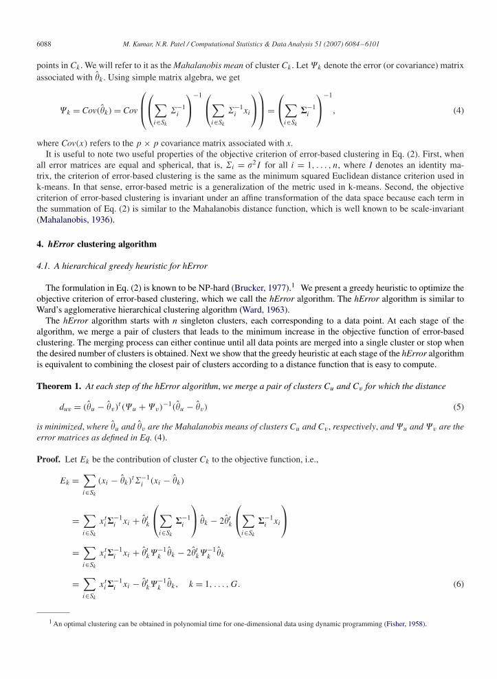
a b

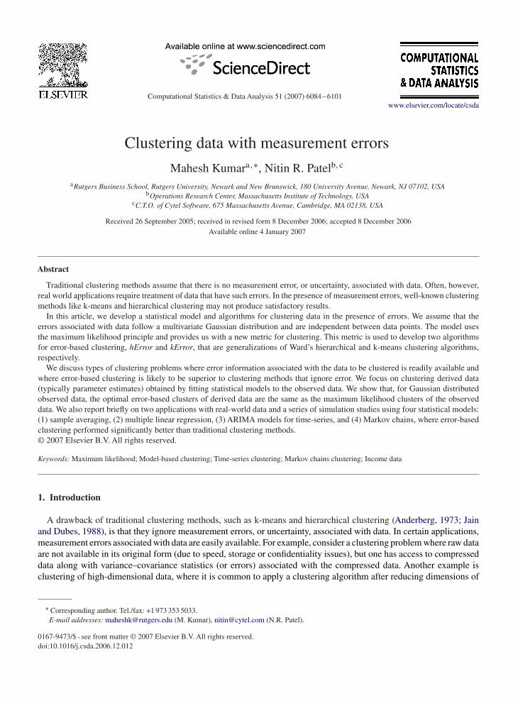
Fig. 1. Clustering data without considering error information. (a) Sample averages for four regions along with standard errors. (b) k-means clusteringbased on sample averages.

A

C

B

D

scaled expenditure scaled expenditure

sca

led

in

co

me

sca

led

in

co

me

A

C

B

D

Cluster 2

Cluster 1

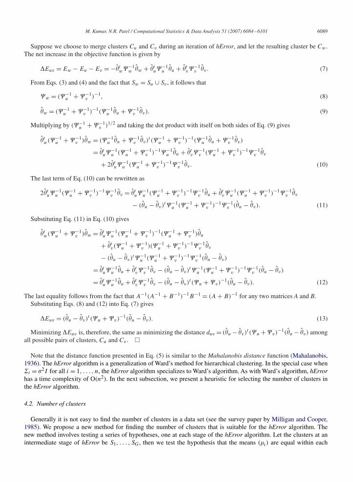
a b

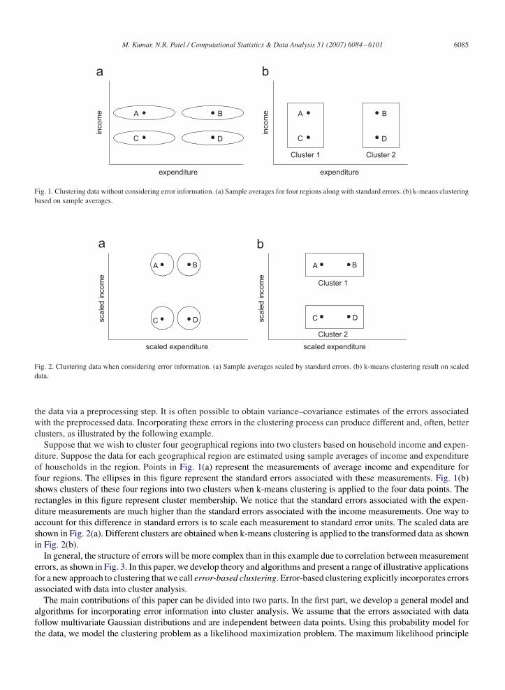
Fig. 2. Clustering data when considering error information. (a) Sample averages scaled by standard errors. (b) k-means clustering result on scaleddata.

the data via a preprocessing step. It is often possible to obtain variance–covariance estimates of the errors associatedwith the preprocessed data. Incorporating these errors in the clustering process can produce different and, often, betterclusters, as illustrated by the following example.

Suppose that we wish to cluster four geographical regions into two clusters based on household income and expen-diture. Suppose the data for each geographical region are estimated using sample averages of income and expenditureof households in the region. Points in Fig. 1(a) represent the measurements of average income and expenditure forfour regions. The ellipses in this figure represent the standard errors associated with these measurements. Fig. 1(b)shows clusters of these four regions into two clusters when k-means clustering is applied to the four data points. Therectangles in this figure represent cluster membership. We notice that the standard errors associated with the expen-diture measurements are much higher than the standard errors associated with the income measurements. One way toaccount for this difference in standard errors is to scale each measurement to standard error units. The scaled data areshown in Fig. 2(a). Different clusters are obtained when k-means clustering is applied to the transformed data as shownin Fig. 2(b).

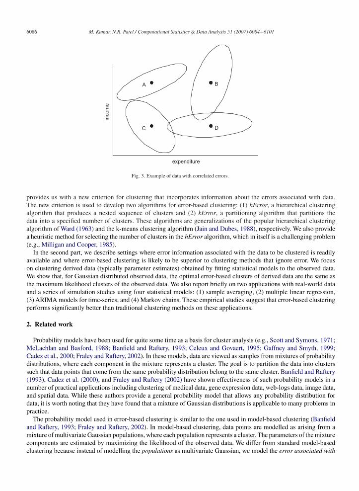
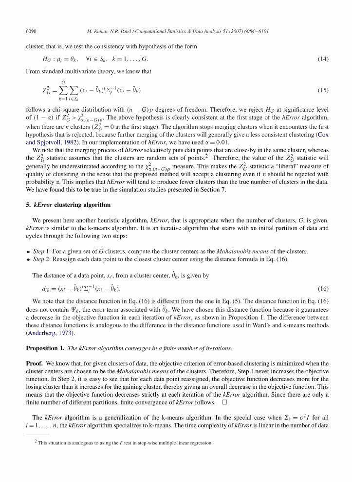
In general, the structure of errors will be more complex than in this example due to correlation between measurementerrors, as shown in Fig. 3. In this paper, we develop theory and algorithms and present a range of illustrative applicationsfor a new approach to clustering that we call error-based clustering. Error-based clustering explicitly incorporates errorsassociated with data into cluster analysis.

The main contributions of this paper can be divided into two parts. In the first part, we develop a general model andalgorithms for incorporating error information into cluster analysis. We assume that the errors associated with datafollow multivariate Gaussian distributions and are independent between data points. Using this probability model forthe data, we model the clustering problem as a likelihood maximization problem. The maximum likelihood principle

6086 M. Kumar, N.R. Patel / Computational Statistics & Data Analysis 51 (2007) 6084–6101

A

C

B

D

expenditure

inco

me

Fig. 3. Example of data with correlated errors.

provides us with a new criterion for clustering that incorporates information about the errors associated with data.The new criterion is used to develop two algorithms for error-based clustering: (1) hError, a hierarchical clusteringalgorithm that produces a nested sequence of clusters and (2) kError, a partitioning algorithm that partitions thedata into a specified number of clusters. These algorithms are generalizations of the popular hierarchical clusteringalgorithm of Ward (1963) and the k-means clustering algorithm (Jain and Dubes, 1988), respectively. We also providea heuristic method for selecting the number of clusters in the hError algorithm, which in itself is a challenging problem(e.g., Milligan and Cooper, 1985).

In the second part, we describe settings where error information associated with the data to be clustered is readilyavailable and where error-based clustering is likely to be superior to clustering methods that ignore error. We focuson clustering derived data (typically parameter estimates) obtained by fitting statistical models to the observed data.We show that, for Gaussian distributed observed data, the optimal error-based clusters of derived data are the same asthe maximum likelihood clusters of the observed data. We also report briefly on two applications with real-world dataand a series of simulation studies using four statistical models: (1) sample averaging, (2) multiple linear regression,(3) ARIMA models for time-series, and (4) Markov chains. These empirical studies suggest that error-based clusteringperforms significantly better than traditional clustering methods on these applications.

2. Related work

Probability models have been used for quite some time as a basis for cluster analysis (e.g., Scott and Symons, 1971;McLachlan and Basford, 1988; Banfield and Raftery, 1993; Celeux and Govaert, 1995; Gaffney and Smyth, 1999;Cadez et al., 2000; Fraley and Raftery, 2002). In these models, data are viewed as samples from mixtures of probabilitydistributions, where each component in the mixture represents a cluster. The goal is to partition the data into clusterssuch that data points that come from the same probability distribution belong to the same cluster. Banfield and Raftery(1993), Cadez et al. (2000), and Fraley and Raftery (2002) have shown effectiveness of such probability models in anumber of practical applications including clustering of medical data, gene expression data, web-logs data, image data,and spatial data. While these authors provide a general probability model that allows any probability distribution fordata, it is worth noting that they have found that a mixture of Gaussian distributions is applicable to many problems inpractice.

The probability model used in error-based clustering is similar to the one used in model-based clustering (Banfieldand Raftery, 1993; Fraley and Raftery, 2002). In model-based clustering, data points are modelled as arising from amixture of multivariate Gaussian populations, where each population represents a cluster. The parameters of the mixturecomponents are estimated by maximizing the likelihood of the observed data. We differ from standard model-basedclustering because instead of modelling the populations as multivariate Gaussian, we model the error associated with


each data point as multivariate Gaussian. In other words, in the special case when it is assumed that all data pointsin the same cluster have the same error distribution, error-based clustering is equivalent to model-based clustering.In that sense, error-based clustering is a generalization of model-based clustering. By allowing different amounts oferror for each data point, error-based clustering explicitly models error information for incorporation into the clusteringalgorithms.

In our literature search, we have come across only one publication (Chaudhuri and Bhowmik, 1998) that explicitlyconsiders error information in multivariate clustering. It provides a heuristic solution for the case of uniformly distributedspherical errors associated with data. We consider the case when errors follow multivariate Gaussian distributions andprovide a formal statistical procedure to model them. Modelling errors using the Gaussian distribution has a longhistory (beginning with Gauss!) and is applicable to many problems in practice (e.g., Sarachik and Grimson, 1993; Fenget al., 1996).

The work of Stanford and Raftery (2000) and Cadez et al. (2000) is similar to the work we have proposed in thispaper. These authors have proposed clustering of individuals that may not have the usual vector representation in afixed dimension. The work in these papers is specific to their applications and is based on the EM algorithm. We haveproposed an alternative approach that is easy to solve computationally and is applicable to a broad class of problems.

While there is almost no prior published work on incorporating error information in multivariate cluster analysis,there has been significant work on this topic for one-dimensional data (e.g., Fisher, 1958; Cox and Spjotvoll, 1982;Cowpertwait and Cox, 1992). Cowpertwait and Cox (1992) applied their technique to clustering univariate slopecoefficients from a group of regressions and used it for predicting rainfall. We extend their work to clustering multivariateregression coefficients.

3. Model for error-based clustering

The data to be clustered consists of n observations x1, . . . , xn (column vectors) inRp and n positive definite matrices�1, . . . ,�n in Rp×p, where xi represents measurements on p characteristics and �i represents the covariance matrixassociated with the observed measurements of xi . Suppose that the data points are independent and that each arisesfrom a p-variate Gaussian distribution with one of G possible means �1, . . . , �G, G�n, that is, xi ∼ Np(�i , �i ), where�i ∈ {�1, . . . , �G} for i=1, . . . , n. Our goal is to find the clusters C1, . . . , CG such that observations that have the samemean (�i ) belong to the same cluster with �i = �k , the common value of �i for the observations in Ck , k = 1, . . . , G.

Let Sk = {i|xi ∈ Ck}, then �i = �k for ∀i ∈ Sk , k = 1, . . . , G. Given data points x1, . . . , xn and the error matrices�1, . . . ,�n, the maximum likelihood principle leads us to choose S = (S1, . . . , SG) and � = (�1, . . . , �G) so as tomaximize the likelihood

L(x|S, �) =G∏

k=1

∏i∈Sk

1

(2�)p2|�i |−1/2 e−1/2(xi−�k)

t�−1i (xi−�k), (1)

where |�i | is the determinant of �i for i = 1, . . . , n. It is easy to show that the likelihood in Eq. (1) is maximum forthe partition S1, . . . , SG that solves

minS1,...,SG

G∑k=1

∑i∈Sk

(xi − �̂k)t�−1

i (xi − �̂k), (2)

where �̂k is the maximum likelihood estimate (MLE) of �k given by

�̂k =⎛⎝∑

i∈Sk

�−1i

⎞⎠

−1 ⎛⎝∑

i∈Sk

�−1i xi

⎞⎠ , k = 1, . . . , G. (3)

The minimization in Eq. (2) makes intuitive sense because each data point is weighted by the inverse of its error,that is, data points with smaller error get higher weight and vice versa. Notice that �̂k is a weighted mean of the data


points in Ck . We will refer to it as the Mahalanobis mean of cluster Ck . Let �k denote the error (or covariance) matrixassociated with �̂k . Using simple matrix algebra, we get

�k = Cov(�̂k) = Cov

⎛⎜⎝

⎛⎝∑

i∈Sk

�−1i

⎞⎠

−1 ⎛⎝∑

i∈Sk

�−1i xi

⎞⎠

⎞⎟⎠ =

⎛⎝∑

i∈Sk

�−1i

⎞⎠

−1

, (4)

where Cov(x) refers to the p × p covariance matrix associated with x.It is useful to note two useful properties of the objective criterion of error-based clustering in Eq. (2). First, when

all error matrices are equal and spherical, that is, �i = �2I for all i = 1, . . . , n, where I denotes an identity ma-trix, the criterion of error-based clustering is the same as the minimum squared Euclidean distance criterion used ink-means. In that sense, error-based metric is a generalization of the metric used in k-means. Second, the objectivecriterion of error-based clustering is invariant under an affine transformation of the data space because each term inthe summation of Eq. (2) is similar to the Mahalanobis distance function, which is well known to be scale-invariant(Mahalanobis, 1936).

4. hError clustering algorithm

4.1. A hierarchical greedy heuristic for hError

The formulation in Eq. (2) is known to be NP-hard (Brucker, 1977).1 We present a greedy heuristic to optimize theobjective criterion of error-based clustering, which we call the hError algorithm. The hError algorithm is similar toWard’s agglomerative hierarchical clustering algorithm (Ward, 1963).

The hError algorithm starts with n singleton clusters, each corresponding to a data point. At each stage of thealgorithm, we merge a pair of clusters that leads to the minimum increase in the objective function of error-basedclustering. The merging process can either continue until all data points are merged into a single cluster or stop whenthe desired number of clusters is obtained. Next we show that the greedy heuristic at each stage of the hError algorithmis equivalent to combining the closest pair of clusters according to a distance function that is easy to compute.

Theorem 1. At each step of the hError algorithm, we merge a pair of clusters Cu and Cv for which the distance

duv = (�̂u − �̂v)t (�u + �v)

−1(�̂u − �̂v) (5)

is minimized, where �̂u and �̂v are the Mahalanobis means of clusters Cu and Cv , respectively, and �u and �v are theerror matrices as defined in Eq. (4).

Proof. Let Ek be the contribution of cluster Ck to the objective function, i.e.,

Ek =∑i∈Sk

(xi − �̂k)t�−1

i (xi − �̂k)

=∑i∈Sk

xti �

−1i xi + �̂t

k

⎛⎝∑

i∈Sk

�−1i

⎞⎠ �̂k − 2�̂t

k

⎛⎝∑

i∈Sk

�−1i xi

⎞⎠

=∑i∈Sk

xti �

−1i xi + �̂t

k�−1k �̂k − 2�̂t

k�−1k �̂k

=∑i∈Sk

xti �

−1i xi − �̂t

k�−1k �̂k, k = 1, . . . , G. (6)

1 An optimal clustering can be obtained in polynomial time for one-dimensional data using dynamic programming (Fisher, 1958).


Suppose we choose to merge clusters Cu and Cv during an iteration of hError, and let the resulting cluster be Cw.The net increase in the objective function is given by

�Euv = Ew − Eu − Ev = −�̂tw�−1

w �̂w + �̂tu�

−1u �̂u + �̂t

v�−1v �̂v . (7)

From Eqs. (3) and (4) and the fact that Sw = Su ∪ Sv , it follows that

�w = (�−1u + �−1

v )−1, (8)

�̂w = (�−1u + �−1

v )−1(�−1u �̂u + �−1

v �̂v). (9)

Multiplying by (�−1u + �−1

v )1/2 and taking the dot product with itself on both sides of Eq. (9) gives

�̂tw(�−1

u + �−1v )�̂w = (�−1

u �̂u + �−1v �̂v)

t (�−1u + �−1

v )−1(�−1u �̂u + �−1

v �̂v)

= �̂tu�

−1u (�−1

u + �−1v )−1�−1

u �̂u + �̂tv�

−1v (�−1

u + �−1v )−1�−1

v �̂v

+ 2�̂tu�

−1u (�−1

u + �−1v )−1�−1

v �̂v . (10)

The last term of Eq. (10) can be rewritten as

2�̂tu�

−1u (�−1

u + �−1v )−1�−1

v �̂v = �̂tu�

−1u (�−1

u + �−1v )−1�−1

v �̂u + �̂tv�

−1u (�−1

u + �−1v )−1�−1

v �̂v

− (�̂u − �̂v)t�−1

u (�−1u + �−1

v )−1�−1v (�̂u − �̂v). (11)

Substituting Eq. (11) in Eq. (10) gives

�̂tw(�−1

u + �−1v )�̂w = �̂t

u�−1u (�−1

u + �−1v )−1(�−1

u + �−1v )�̂u

+ �̂tv(�

−1u + �−1

v )(�−1u + �−1

v )−1�−1v �̂v

− (�̂u − �̂v)t�−1

u (�−1u + �−1

v )−1�−1v (�̂u − �̂v)

= �̂tu�

−1u �̂u + �̂t

v�−1v �̂v − (�̂u − �̂v)

t�−1u (�−1

u + �−1v )−1�−1

v (�̂u − �̂v)

= �̂tu�

−1u �̂u + �̂t

v�−1v �̂v − (�̂u − �̂v)

t (�u + �v)−1(�̂u − �̂v). (12)

The last equality follows from the fact that A−1(A−1 + B−1)−1B−1 = (A + B)−1 for any two matrices A and B.Substituting Eqs. (8) and (12) into Eq. (7) gives

�Euv = (�̂u − �̂v)t (�u + �v)

−1(�̂u − �̂v). (13)

Minimizing �Euv is, therefore, the same as minimizing the distance duv = (�̂u − �̂v)t (�u +�v)

−1(�̂u − �̂v) amongall possible pairs of clusters, Cu and Cv . �

Note that the distance function presented in Eq. (5) is similar to the Mahalanobis distance function (Mahalanobis,1936). The hError algorithm is a generalization of Ward’s method for hierarchical clustering. In the special case when�i = �2I for all i = 1, . . . , n, the hError algorithm specializes to Ward’s algorithm. As with Ward’s algorithm, hErrorhas a time complexity of O(n2). In the next subsection, we present a heuristic for selecting the number of clusters inthe hError algorithm.

4.2. Number of clusters

Generally it is not easy to find the number of clusters in a data set (see the survey paper by Milligan and Cooper,1985). We propose a new method for finding the number of clusters that is suitable for the hError algorithm. Thenew method involves testing a series of hypotheses, one at each stage of the hError algorithm. Let the clusters at anintermediate stage of hError be S1, . . . , SG, then we test the hypothesis that the means (�i ) are equal within each


cluster, that is, we test the consistency with hypothesis of the form

HG : �i = �k, ∀i ∈ Sk, k = 1, . . . , G. (14)

From standard multivariate theory, we know that

Z2G =

G∑k=1

∑i∈Sk

(xi − �̂k)t�−1

i (xi − �̂k) (15)

follows a chi-square distribution with (n − G)p degrees of freedom. Therefore, we reject HG at significance levelof (1 − �) if Z2

G > 2�,(n−G)p. The above hypothesis is clearly consistent at the first stage of the hError algorithm,

when there are n clusters (Z2G = 0 at the first stage). The algorithm stops merging clusters when it encounters the first

hypothesis that is rejected, because further merging of the clusters will generally give a less consistent clustering (Coxand Spjotvoll, 1982). In our implementation of hError, we have used � = 0.01.

We note that the merging process of hError selectively puts data points that are close-by in the same cluster, whereasthe Z2

G statistic assumes that the clusters are random sets of points.2 Therefore, the value of the Z2G statistic will

generally be underestimated according to the 2�,(n−G)p measure. This makes the Z2

G statistic a “liberal” measure ofquality of clustering in the sense that the proposed method will accept a clustering even if it should be rejected withprobability �. This implies that hError will tend to produce fewer clusters than the true number of clusters in the data.We have found this to be true in the simulation studies presented in Section 7.

5. kError clustering algorithm

We present here another heuristic algorithm, kError, that is appropriate when the number of clusters, G, is given.kError is similar to the k-means algorithm. It is an iterative algorithm that starts with an initial partition of data andcycles through the following two steps:

• Step 1: For a given set of G clusters, compute the cluster centers as the Mahalanobis means of the clusters.• Step 2: Reassign each data point to the closest cluster center using the distance formula in Eq. (16).

The distance of a data point, xi , from a cluster center, �̂k , is given by

dik = (xi − �̂k)t�−1

i (xi − �̂k). (16)

We note that the distance function in Eq. (16) is different from the one in Eq. (5). The distance function in Eq. (16)does not contain �k , the error term associated with �̂k . We have chosen this distance function because it guaranteesa decrease in the objective function in each iteration of kError, as shown in Proposition 1. The difference betweenthese distance functions is analogous to the difference in the distance functions used in Ward’s and k-means methods(Anderberg, 1973).

Proposition 1. The kError algorithm converges in a finite number of iterations.

Proof. We know that, for given clusters of data, the objective criterion of error-based clustering is minimized when thecluster centers are chosen to be the Mahalanobis means of the clusters. Therefore, Step 1 never increases the objectivefunction. In Step 2, it is easy to see that for each data point reassigned, the objective function decreases more for thelosing cluster than it increases for the gaining cluster, thereby giving an overall decrease in the objective function. Thismeans that the objective function decreases strictly at each iteration of the kError algorithm. Since there are only afinite number of different partitions, finite convergence of kError follows. �

The kError algorithm is a generalization of the k-means algorithm. In the special case when �i = �2I for alli =1, . . . , n, the kError algorithm specializes to k-means. The time complexity of kError is linear in the number of data

2 This situation is analogous to using the F test in step-wise multiple linear regression.


points and the number of iterations the algorithm makes. In our empirical studies, we have found that the algorithmgenerally converges after a few iterations (typically less than 10 iterations); therefore, kError is generally faster thanthe hError algorithm. On the other hand, kError requires a priori specification of the number of clusters.

A drawback of the kError algorithm is that the final clusters may depend on the initial partition. It can also produceempty clusters if all points in a cluster are reassigned to other clusters, thereby reducing the number of clusters. Thek-means algorithm also has these shortcomings (Pena et al., 1999). We propose the following solution that is similar tothe one that is often used in k-means. Run the kError algorithm a large number of times with different random initialpartitions and pick the one that has the least value of the objective function. We ignore those solutions that contain oneor more empty clusters. Pena et al. (1999) have shown that, if k-means is run a large number of times, the resultingclusters will be close to optimal and insensitive to the initial partition. In our empirical studies, we have found that thisis also true for kError.

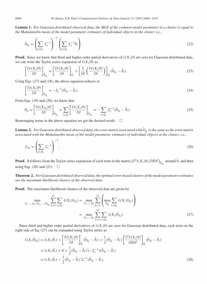
6. Clustering model parameters using error-based clustering

In this section, we present a class of clustering problems where error information about data to be clustered is readilyavailable and where error-based clustering results are typically superior to standard clustering methods that ignore errorinformation. We focus on clustering problems where the objects to be clustered (observed data) are modelled usingstatistical models. Each object in this case is identified by the parameters of a statistical model. A commonly usedmethod for estimating the parameters of statistical models is the maximum likelihood method, which also providesthe covariance matrix (or error information) associated with the estimates of the model parameters. If we wish tocluster these objects on the basis of the model parameter estimates, then error-based clustering becomes a naturalchoice of clustering method. We must note that while covariance matrices are estimated in this application, error-basedclustering assumes that covariance matrices are given. This kind of approximation is common in statistics literatureto simplify the model. A central result of this paper is that, if the observed data are Gaussian distributed, then theoptimal error-based clusters of the estimated model parameters are the same as the maximum likelihood clusters of theobserved data.

6.1. Motivation for clustering model parameters

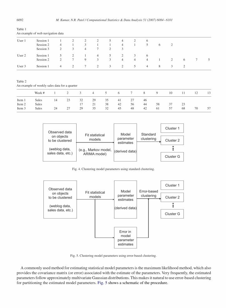
Clustering algorithms typically assume that the data to be clustered is available in a vector form in fixed dimensions.For example, given p measurements on a set of individuals, we represent each individual by a p-dimensional vectorconsisting of these measurements. However, there are many clustering problems when individuals to be clustered donot have an obvious representation as vectors in a fixed dimension. Examples include clustering time-series data andclustering individuals based on web browsing behavior (see Cadez and Smyth, 1999; Cadez et al., 2000; Tong andDabas, 1990 for more examples). Tables 1 and 2 show two examples of such data.

The first table contains sequences of web page requests made by three users on a web site, where each web page isidentified by a unique page number. The second table contains sales data for three items, where each item is sold overdifferent weeks. We would like to cluster these users (or items) based on their web navigation patterns (or sales data),but it is not clear how to obtain such clusters using standard clustering techniques.

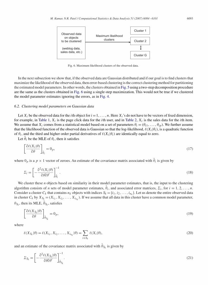
Piccolo (1990), Cadez and Smyth (1999), Cadez et al. (2000), and Maharaj (2000) have shown that the data to beclustered in these examples can be transformed to a fixed dimension vector representation via a preprocessing step. Bymodelling the data for each object as coming from a statistical model (for example, a Markov chain model for eachuser in the web navigation example and an ARIMA time-series model for each item in the sales data example), thepreprocessing step generates a set of vectors (one vector for each object) of model parameters of fixed dimension.3 Thenthe objects can be clustered based on similarity between the vectors of estimated parameters using standard clusteringtechniques, as shown in Fig. 4. The work by Piccolo (1990) on clustering of time-series is an example of the methodshown in Fig. 4.

3 The estimated model parameters are in much smaller dimension than the observed data. Thus it provides a natural way to reduce dimensionsof the observed data.


Table 1An example of web navigation data

User 1 Session 1 1 2 2 2 5 4 2 6Session 2 4 1 3 1 1 4 1 5 6 2Session 3 2 3 4 7 2 3

User 2 Session 1 5 2 1 4 5 2 3 6Session 2 2 7 9 3 3 4 4 4 1 2 6 7 5

User 3 Session 1 4 2 7 2 3 2 5 4 8 3 2

Table 2An example of weekly sales data for a quarter

Week # 1 2 3 4 5 6 7 8 9 10 11 12 13

Item 1 Sales 14 23 32 29 35 41 27 46Item 2 Sales 17 21 38 42 56 44 58 37 23Item 3 Sales 24 27 29 35 32 45 48 42 61 57 68 70 57

Observed data

on objectsto be clustered

(weblog data,sales data, etc.)

Modelparameterestimates

(derived data)

Cluster 1

Cluster 2

Cluster G

...

Fit statistical

models

(e.g., Markov model,ARIMA model)

Standard

clustering

Fig. 4. Clustering model parameters using standard clustering.

Observed data



Modelparameterestimates

(derived data)

Cluster 1

Cluster 2

Cluster G

...

Fit statistical

models

Error-based

clustering

Error inmodel

parameter

estimates

Fig. 5. Clustering model parameters using error-based clustering.

A commonly used method for estimating statistical model parameters is the maximum likelihood method, which alsoprovides the covariance matrix (or error) associated with the estimate of the parameters. Very frequently, the estimatedparameters follow approximately multivariate Gaussian distributions. This makes it natural to use error-based clusteringfor partitioning the estimated model parameters. Fig. 5 shows a schematic of the procedure.


Observed data



Cluster 1

Cluster 2

Cluster G

...

Maximum likelihood

clusters

Fig. 6. Maximum likelihood clusters of the observed data.

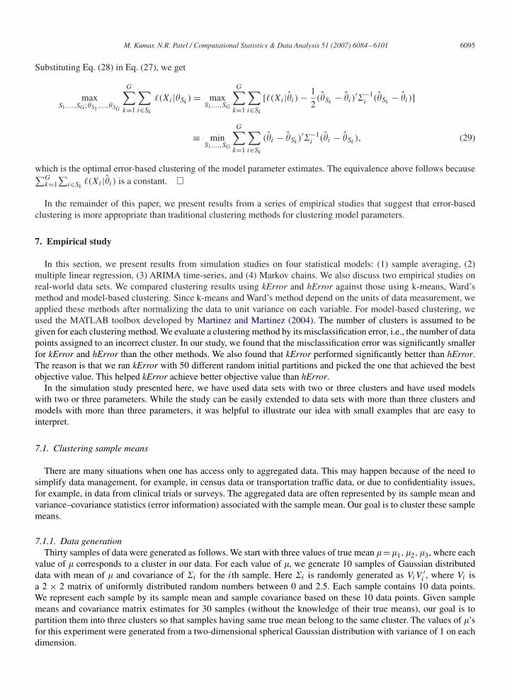
In the next subsection we show that, if the observed data are Gaussian distributed and if our goal is to find clusters thatmaximize the likelihood of the observed data, then error-based clustering is the correct clustering method for partitioningthe estimated model parameters. In other words, the clusters obtained in Fig. 5 using a two-step decomposition procedureare the same as the clusters obtained in Fig. 6 using a single-step maximization. This would not be true if we clusteredthe model parameter estimates ignoring the errors, as in Fig. 4.

6.2. Clustering model parameters on Gaussian data

Let Xi be the observed data for the ith object for i =1, . . . , n. Here Xi’s do not have to be vectors of fixed dimension,for example, in Table 1, Xi is the page click data for the ith user, and in Table 2, Xi is the sales data for the ith item.We assume that Xi comes from a statistical model based on a set of parameters �i = (�i1, . . . , �ip). We further assumethat the likelihood function of the observed data is Gaussian so that the log-likelihood, �(Xi |�i ), is a quadratic functionof �i , and the third and higher order partial derivatives of �(Xi |�i ) are identically equal to zero.

Let �̂i be the MLE of �i , then it satisfies[��(Xi |�)

��

]�̂i

= 0p, (17)

where 0p is a p × 1 vector of zeroes. An estimate of the covariance matrix associated with �̂i is given by

�i =[−�2�(Xi |�)

��′]−1

�̂i

. (18)

We cluster these n objects based on similarity in their model parameter estimates, that is, the input to the clusteringalgorithm consists of n sets of model parameter estimates, �̂i , and associated error matrices, �i , for i = 1, 2, . . . , n.Consider a cluster Ck that contains nk objects with indices Sk ={i1, i2, . . . , ink

}. Let us denote the entire observed datain cluster Ck by XSk

= (Xi1 , Xi2 , . . . , Xink). If we assume that all data in this cluster have a common model parameter,

�Sk, then its MLE, �̂Sk

, satisfies[��(XSk

|�)

��

]�̂Sk

= 0p, (19)

where

�(XSk|�) = �(Xi1 , Xi2 , . . . , Xink

|�) =∑i∈Sk

�(Xi |�), (20)

and an estimate of the covariance matrix associated with �̂Skis given by

�Sk=

[−�2�(XSk

|�)

��′]−1

�̂Sk

. (21)


Lemma 1. For Gaussian distributed observed data, the MLE of the common model parameter in a cluster is equal tothe Mahalanobis mean of the model parameter estimates of individual objects in the cluster, i.e.,

�̂Sk=

⎛⎝∑

i∈Sk

�−1i

⎞⎠

−1 ⎛⎝∑

i∈Sk

�−1i �̂i

⎞⎠ . (22)

Proof. Since we know that third and higher order partial derivatives of �(Xi |�) are zero for Gaussian distributed data,we can write the Taylor series expansion of �(Xi |�) as[

��(Xi |�)

��

]�̂Sk

=[��(Xi |�)

��

]�̂i

+[

�

��

(��(Xi |�)

��

)]�̂i

(�̂Sk− �̂i ). (23)

Using Eqs. (17) and (18), the above equation reduces to[��(Xi |�)

��

]�̂Sk

= −�−1i (�̂Sk

− �̂i ). (24)

From Eqs. (19) and (20), we know that

0p =[��(XSk

|�)

��

]�̂Sk

=∑i∈Sk

[��(Xi |�)

��

]�̂Sk

= −∑i∈Sk

�−1i (�̂Sk

− �̂i ). (25)

Rearranging terms in the above equation we get the desired result. �

Lemma 2. For Gaussian distributed observed data, the error matrix associated with �̂Skis the same as the error matrix

associated with the Mahalanobis mean of the model parameter estimates of individual objects in the cluster, i.e.,

�Sk=

⎛⎝∑

i∈Sk

�−1i

⎞⎠

−1

. (26)

Proof. It follows from the Taylor series expansion of each term in the matrix [�2�(Xi |�)/��′]�̂Sk

around �̂i and then

using Eqs. (20) and (21). �

Theorem 2. For Gaussian distributed observed data, the optimal error-based clusters of the model parameter estimatesare the maximum likelihood clusters of the observed data.

Proof. The maximum likelihood clusters of the observed data are given by

maxS1,...,SG;�S1 ,...,�SG

G∑k=1

∑i∈Sk

�(Xi |�Sk) = max

S1,...,SG

G∑k=1

⎛⎝max

�Sk

∑i∈Sk

�(Xi |�Sk)

⎞⎠

= maxS1,...,SG

G∑k=1

∑i∈Sk

�(Xi |�̂Sk). (27)

Since third and higher order partial derivatives of �(Xi |�) are zero for Gaussian distributed data, each term on theright side of Eq. (27) can be expanded using Taylor series as

�(Xi |�̂Sk) = �(Xi |�̂i ) +

[��(Xi |�)

��

]′

�̂i

(�̂Sk− �̂i ) + 1

2(�̂Sk

− �̂i )′[�2�(Xi |�)

��′]

�̂i

(�̂Sk− �̂i )

= �(Xi |�̂i ) + 0 + 1

2(�̂Sk

− �̂i )′(−�−1

i )(�̂Sk− �̂i )

= �(Xi |�̂i ) − 1

2(�̂Sk

− �̂i )′�−1

i (�̂Sk− �̂i ). (28)


Substituting Eq. (28) in Eq. (27), we get

maxS1,...,SG;�S1 ,...,�SG

G∑k=1

∑i∈Sk

�(Xi |�Sk) = max

S1,...,SG

G∑k=1

∑i∈Sk

[�(Xi |�̂i ) − 1

2(�̂Sk

− �̂i )′�−1

i (�̂Sk− �̂i )]

≡ minS1,...,SG

G∑k=1

∑i∈Sk

(�̂i − �̂Sk)′�−1

i (�̂i − �̂Sk), (29)

which is the optimal error-based clustering of the model parameter estimates. The equivalence above follows because∑Gk=1

∑i∈Sk

�(Xi |�̂i ) is a constant. �

In the remainder of this paper, we present results from a series of empirical studies that suggest that error-basedclustering is more appropriate than traditional clustering methods for clustering model parameters.

7. Empirical study

In this section, we present results from simulation studies on four statistical models: (1) sample averaging, (2)multiple linear regression, (3) ARIMA time-series, and (4) Markov chains. We also discuss two empirical studies onreal-world data sets. We compared clustering results using kError and hError against those using k-means, Ward’smethod and model-based clustering. Since k-means and Ward’s method depend on the units of data measurement, weapplied these methods after normalizing the data to unit variance on each variable. For model-based clustering, weused the MATLAB toolbox developed by Martinez and Martinez (2004). The number of clusters is assumed to begiven for each clustering method. We evaluate a clustering method by its misclassification error, i.e., the number of datapoints assigned to an incorrect cluster. In our study, we found that the misclassification error was significantly smallerfor kError and hError than the other methods. We also found that kError performed significantly better than hError.The reason is that we ran kError with 50 different random initial partitions and picked the one that achieved the bestobjective value. This helped kError achieve better objective value than hError.

In the simulation study presented here, we have used data sets with two or three clusters and have used modelswith two or three parameters. While the study can be easily extended to data sets with more than three clusters andmodels with more than three parameters, it was helpful to illustrate our idea with small examples that are easy tointerpret.

7.1. Clustering sample means

There are many situations when one has access only to aggregated data. This may happen because of the need tosimplify data management, for example, in census data or transportation traffic data, or due to confidentiality issues,for example, in data from clinical trials or surveys. The aggregated data are often represented by its sample mean andvariance–covariance statistics (error information) associated with the sample mean. Our goal is to cluster these samplemeans.

7.1.1. Data generationThirty samples of data were generated as follows. We start with three values of true mean �=�1, �2, �3, where each

value of � corresponds to a cluster in our data. For each value of �, we generate 10 samples of Gaussian distributeddata with mean of � and covariance of �i for the ith sample. Here �i is randomly generated as ViV

′i , where Vi is

a 2 × 2 matrix of uniformly distributed random numbers between 0 and 2.5. Each sample contains 10 data points.We represent each sample by its sample mean and sample covariance based on these 10 data points. Given samplemeans and covariance matrix estimates for 30 samples (without the knowledge of their true means), our goal is topartition them into three clusters so that samples having same true mean belong to the same cluster. The values of �’sfor this experiment were generated from a two-dimensional spherical Gaussian distribution with variance of 1 on eachdimension.


Table 3Average misclassification error for clustering of sample means

Clustering method Average misclassification error

kError 3.45 (0.32)hError 4.52 (0.34)Model-based 8.20 (0.48)k-means 8.02 (0.41)Ward 12.25 (0.45)

Table 4Misclassification error with diagonal approximation for sample covariance


kError with diagonal approximation 6.67 (0.41)hError with diagonal approximation 6.99 (0.42)

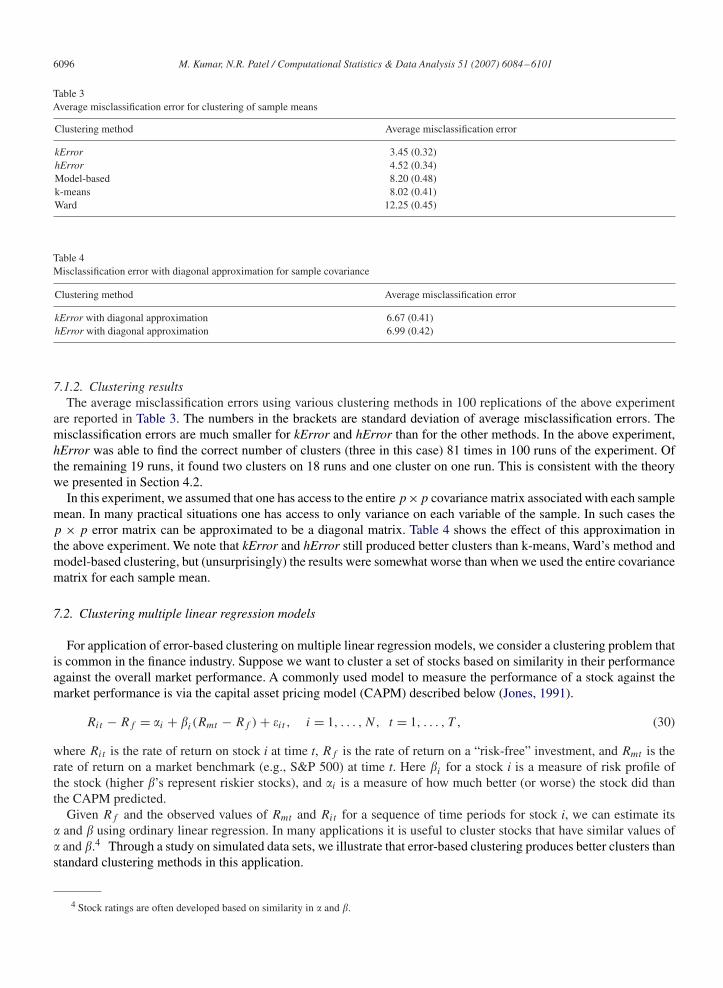
7.1.2. Clustering resultsThe average misclassification errors using various clustering methods in 100 replications of the above experiment

are reported in Table 3. The numbers in the brackets are standard deviation of average misclassification errors. Themisclassification errors are much smaller for kError and hError than for the other methods. In the above experiment,hError was able to find the correct number of clusters (three in this case) 81 times in 100 runs of the experiment. Ofthe remaining 19 runs, it found two clusters on 18 runs and one cluster on one run. This is consistent with the theorywe presented in Section 4.2.

In this experiment, we assumed that one has access to the entire p×p covariance matrix associated with each samplemean. In many practical situations one has access to only variance on each variable of the sample. In such cases thep × p error matrix can be approximated to be a diagonal matrix. Table 4 shows the effect of this approximation inthe above experiment. We note that kError and hError still produced better clusters than k-means, Ward’s method andmodel-based clustering, but (unsurprisingly) the results were somewhat worse than when we used the entire covariancematrix for each sample mean.

7.2. Clustering multiple linear regression models

For application of error-based clustering on multiple linear regression models, we consider a clustering problem thatis common in the finance industry. Suppose we want to cluster a set of stocks based on similarity in their performanceagainst the overall market performance. A commonly used model to measure the performance of a stock against themarket performance is via the capital asset pricing model (CAPM) described below (Jones, 1991).

Rit − Rf = �i + i (Rmt − Rf ) + �it , i = 1, . . . , N, t = 1, . . . , T , (30)

where Rit is the rate of return on stock i at time t, Rf is the rate of return on a “risk-free” investment, and Rmt is therate of return on a market benchmark (e.g., S&P 500) at time t. Here i for a stock i is a measure of risk profile ofthe stock (higher ’s represent riskier stocks), and �i is a measure of how much better (or worse) the stock did thanthe CAPM predicted.

Given Rf and the observed values of Rmt and Rit for a sequence of time periods for stock i, we can estimate its� and using ordinary linear regression. In many applications it is useful to cluster stocks that have similar values of� and .4 Through a study on simulated data sets, we illustrate that error-based clustering produces better clusters thanstandard clustering methods in this application.

4 Stock ratings are often developed based on similarity in � and .


Table 5Average misclassification error for clustering regression models


kError 1.50 (0.28)hError 1.64 (0.31)Model-based 7.02 (0.61)k-means 7.63 (0.36)Ward 11.70 (0.39)k-means on observed data 13.51 (0.21)Ward on observed data 13.96 (0.20)

7.2.1. Data generationWe generated data for 30 stocks as follows. We start with three values of (�, ) that are generated from a two-

dimensional spherical Gaussian distribution with variance of 1 on each dimension. The three values of (�, ) correspondto three clusters of stock. For each value of (�, ), we generate data for 10 stocks as follows. For each stock, we generateits return in 10 time periods using Eq. (30), where Rmt is randomly generated from a uniform distribution between 3%and 8%, �it is generated from a normal distribution N(0, 1), and Rf is taken to be zero. Given stock return and marketreturn data for 30 stocks, our goal is to partition them into three clusters so that stocks that have common values of(�, ) belong to the same cluster.

Given data for 10 time periods for a stock, its (�, ) is estimated using the least square method. Let the estimate be(�̂i , ̂i ) and associated covariance matrix be �i , for the ith stock, i =1, . . . , 30. This constitutes the data to be clustered.

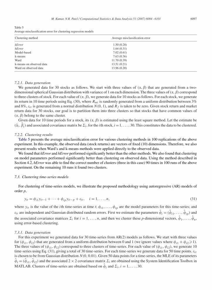
7.2.2. Clustering resultsTable 5 presents the average misclassification error for various clustering methods in 100 replications of the above

experiment. In this example, the observed data (stock returns) are vectors of fixed (10) dimensions. Therefore, we alsopresent results when Ward’s and k-means methods were applied directly to the observed data.

We found that kError and hError performed significantly better than the other methods. We also found that clusteringon model parameters performed significantly better than clustering on observed data. Using the method described inSection 4.2, hError was able to find the correct number of clusters (three in this case) 90 times in 100 runs of the aboveexperiment. On the remaining 10 runs it found two clusters.

7.3. Clustering time-series models

For clustering of time-series models, we illustrate the proposed methodology using autoregressive (AR) models oforder p,

yit = �i1yit−1 + · · · + �ipyit−p + �it , i = 1, . . . , n, (31)

where yit is the value of the ith time-series at time t; �i1, . . . ,�ip are the model parameters for this time-series; and

�it are independent and Gaussian distributed random errors. First we estimate the parameters �̂i = (�̂i1, . . . , �̂ip) and

the associated covariance matrices �i for i = 1, . . . , n, and then we cluster these p-dimensional vectors, �̂1, . . . , �̂n,using error-based clustering.

7.3.1. Data generationFor this experiment we generated data for 30 time-series from AR(2) models as follows. We start with three values

for (�i1, �i2) that are generated from a uniform distribution between 0 and 1 (we ignore values where �i1 + �i2 �1).The three values of (�i1, �i2) correspond to three clusters of time-series. For each value of (�i1, �i2), we generate 10time-series using Eq. (31), giving a total of 30 time-series. For each time-series we generate data for 50 time points. �itis chosen to be from Gaussian distribution N(0, 0.01). Given 50 data points for a time-series, the MLE of its parameters�̂i = (�̂i1, �̂i2) and the associated 2 × 2 covariance matrix �i are obtained using the System Identification Toolbox inMATLAB. Clusters of time-series are obtained based on �̂i and �i , i = 1, . . . , 30.


Table 6Average misclassification error for clustering of time-series models


kError 6.32 (0.36)hError 6.89 (0.38)Model-based 8.49 (0.40)k-means 7.78 (0.39)Ward 10.91 (0.43)k-means on observed data 15.58 (0.17)Ward on observed data 18.21 (0.10)

ShoppingCart

PlaceOrder

Start

Exit

1−p2− p31− p1

p1 p2

p3

Fig. 7. Markov chain model for online users.

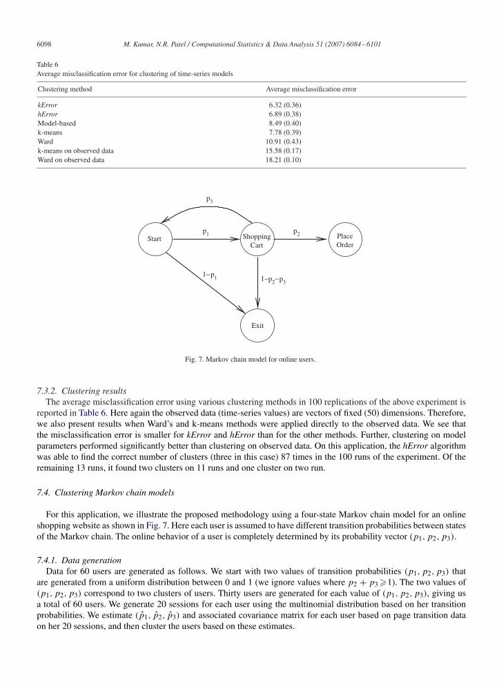
7.3.2. Clustering resultsThe average misclassification error using various clustering methods in 100 replications of the above experiment is

reported in Table 6. Here again the observed data (time-series values) are vectors of fixed (50) dimensions. Therefore,we also present results when Ward’s and k-means methods were applied directly to the observed data. We see thatthe misclassification error is smaller for kError and hError than for the other methods. Further, clustering on modelparameters performed significantly better than clustering on observed data. On this application, the hError algorithmwas able to find the correct number of clusters (three in this case) 87 times in the 100 runs of the experiment. Of theremaining 13 runs, it found two clusters on 11 runs and one cluster on two run.

7.4. Clustering Markov chain models

For this application, we illustrate the proposed methodology using a four-state Markov chain model for an onlineshopping website as shown in Fig. 7. Here each user is assumed to have different transition probabilities between statesof the Markov chain. The online behavior of a user is completely determined by its probability vector (p1, p2, p3).

7.4.1. Data generationData for 60 users are generated as follows. We start with two values of transition probabilities (p1, p2, p3) that

are generated from a uniform distribution between 0 and 1 (we ignore values where p2 + p3 �1). The two values of(p1, p2, p3) correspond to two clusters of users. Thirty users are generated for each value of (p1, p2, p3), giving usa total of 60 users. We generate 20 sessions for each user using the multinomial distribution based on her transitionprobabilities. We estimate (p̂1, p̂2, p̂3) and associated covariance matrix for each user based on page transition dataon her 20 sessions, and then cluster the users based on these estimates.


Table 7Average misclassification error for clustering of Markov chain models


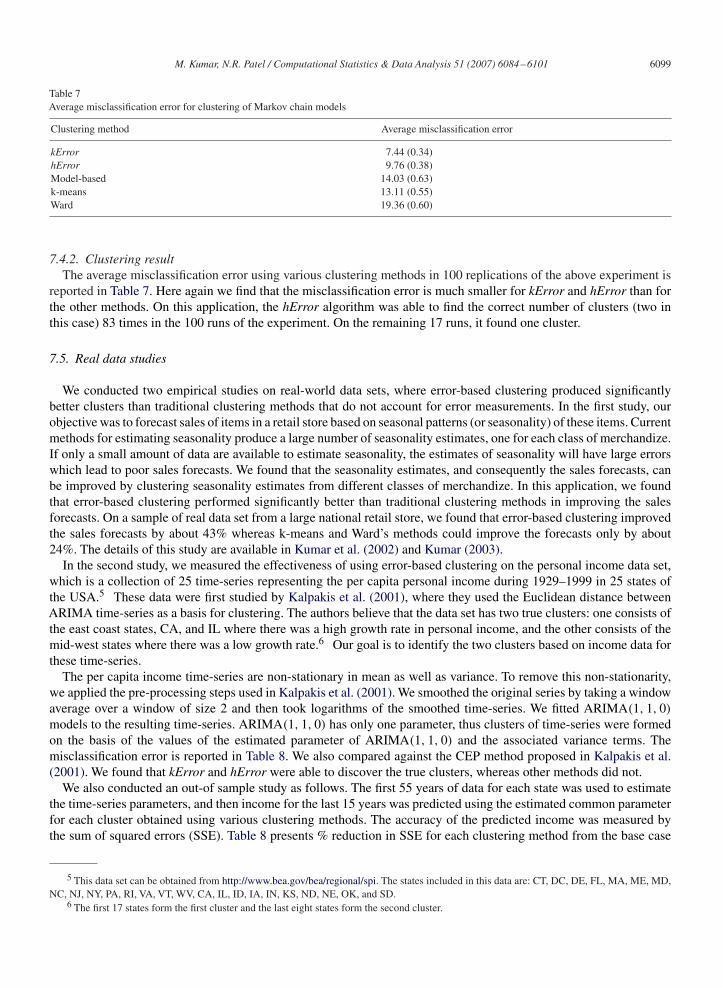
kError 7.44 (0.34)hError 9.76 (0.38)Model-based 14.03 (0.63)k-means 13.11 (0.55)Ward 19.36 (0.60)

7.4.2. Clustering resultThe average misclassification error using various clustering methods in 100 replications of the above experiment is

reported in Table 7. Here again we find that the misclassification error is much smaller for kError and hError than forthe other methods. On this application, the hError algorithm was able to find the correct number of clusters (two inthis case) 83 times in the 100 runs of the experiment. On the remaining 17 runs, it found one cluster.

7.5. Real data studies

We conducted two empirical studies on real-world data sets, where error-based clustering produced significantlybetter clusters than traditional clustering methods that do not account for error measurements. In the first study, ourobjective was to forecast sales of items in a retail store based on seasonal patterns (or seasonality) of these items. Currentmethods for estimating seasonality produce a large number of seasonality estimates, one for each class of merchandize.If only a small amount of data are available to estimate seasonality, the estimates of seasonality will have large errorswhich lead to poor sales forecasts. We found that the seasonality estimates, and consequently the sales forecasts, canbe improved by clustering seasonality estimates from different classes of merchandize. In this application, we foundthat error-based clustering performed significantly better than traditional clustering methods in improving the salesforecasts. On a sample of real data set from a large national retail store, we found that error-based clustering improvedthe sales forecasts by about 43% whereas k-means and Ward’s methods could improve the forecasts only by about24%. The details of this study are available in Kumar et al. (2002) and Kumar (2003).

In the second study, we measured the effectiveness of using error-based clustering on the personal income data set,which is a collection of 25 time-series representing the per capita personal income during 1929–1999 in 25 states ofthe USA.5 These data were first studied by Kalpakis et al. (2001), where they used the Euclidean distance betweenARIMA time-series as a basis for clustering. The authors believe that the data set has two true clusters: one consists ofthe east coast states, CA, and IL where there was a high growth rate in personal income, and the other consists of themid-west states where there was a low growth rate.6 Our goal is to identify the two clusters based on income data forthese time-series.

The per capita income time-series are non-stationary in mean as well as variance. To remove this non-stationarity,we applied the pre-processing steps used in Kalpakis et al. (2001). We smoothed the original series by taking a windowaverage over a window of size 2 and then took logarithms of the smoothed time-series. We fitted ARIMA(1, 1, 0)

models to the resulting time-series. ARIMA(1, 1, 0) has only one parameter, thus clusters of time-series were formedon the basis of the values of the estimated parameter of ARIMA(1, 1, 0) and the associated variance terms. Themisclassification error is reported in Table 8. We also compared against the CEP method proposed in Kalpakis et al.(2001). We found that kError and hError were able to discover the true clusters, whereas other methods did not.

We also conducted an out-of sample study as follows. The first 55 years of data for each state was used to estimatethe time-series parameters, and then income for the last 15 years was predicted using the estimated common parameterfor each cluster obtained using various clustering methods. The accuracy of the predicted income was measured bythe sum of squared errors (SSE). Table 8 presents % reduction in SSE for each clustering method from the base case

5 This data set can be obtained from http://www.bea.gov/bea/regional/spi. The states included in this data are: CT, DC, DE, FL, MA, ME, MD,NC, NJ, NY, PA, RI, VA, VT, WV, CA, IL, ID, IA, IN, KS, ND, NE, OK, and SD.

6 The first 17 states form the first cluster and the last eight states form the second cluster.

http://www.bea.gov/bea/regional/spi


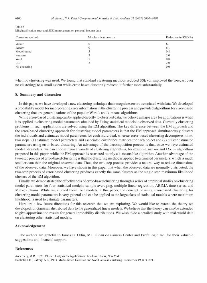
Table 8Misclassification error and SSE improvement on personal income data

Clustering method Misclassification error Reduction in SSE (%)

kError 0 6.1hError 0 6.1Model-based 5 0.8k-means 3 2.0Ward 5 0.8CEP 3 2.0No clustering – 0.0

when no clustering was used. We found that standard clustering methods reduced SSE (or improved the forecast overno clustering) to a small extent while error-based clustering reduced it further more substantially.

8. Summary and discussion

In this paper, we have developed a new clustering technique that recognizes errors associated with data. We developeda probability model for incorporating error information in the clustering process and provided algorithms for error-basedclustering that are generalizations of the popular Ward’s and k-means algorithms.

While error-based clustering can be applied directly to observed data, we believe a major area for applications is whenit is applied to clustering model parameters obtained by fitting statistical models to observed data. Currently clusteringproblems in such applications are solved using the EM algorithm. The key difference between the EM approach andthe error-based clustering approach for clustering model parameters is that the EM approach simultaneously clustersthe individuals and estimates model parameters for each individual, whereas error-based clustering decomposes it intotwo steps: (1) estimate model parameters and associated covariance matrices for each object and (2) cluster estimatedparameters using error-based clustering. An advantage of the decomposition process is that, once we have estimatedmodel parameters, we can choose from a variety of clustering algorithms, for example, hError and kError algorithmsproposed in this paper, while the EM approach is restricted to only a k-means like algorithm. Another advantage of thetwo-step process of error-based clustering is that the clustering method is applied to estimated parameters, which is muchsmaller data than the original observed data. Thus, the two-step process provides a natural way to reduce dimensionsof the observed data. Moreover, we have shown in this paper that when the observed data are normally distributed, thetwo-step process of error-based clustering produces exactly the same clusters as the single step maximum likelihoodclusters of the EM algorithm.

Finally, we demonstrated the effectiveness of error-based clustering through a series of empirical studies on clusteringmodel parameters for four statistical models: sample averaging, multiple linear regression, ARIMA time-series, andMarkov chains. While we studied these four models in this paper, the concept of using error-based clustering forclustering model parameters is very general and can be applied to the large class of statistical models where maximumlikelihood is used to estimate parameters.

Here are a few future directions for this research that we are exploring. We would like to extend the theory wedeveloped for Gaussian distributed data to the generalized linear models. We believe that the theory can also be extendedto give approximation results for general probability distributions. We wish to do a detailed study with real-world dataon clustering other statistical models.

Acknowledgement

The authors are grateful to James B. Orlin, MIT Sloan e-Business Center and ProfitLogic Inc. for their valuablesuggestions and financial support.

References

Anderberg, M.R., 1973. Cluster Analysis for Applications. Academic Press, New York.Banfield, J.D., Raftery, A.E., 1993. Model-based Gaussian and Non-Gaussian clustering. Biometrics 49, 803–821.


Brucker, P., 1977. On the Complexity of Clustering Problems. Optimization and Operations Research. Springer, Berlin. pp. 45–54.Cadez, I., Smyth, P., 1999. Probabilistic clustering using hierarchical models. ICS Technical Report, UC Irvine, pp. 99–116.Cadez, I., Gaffney, S., Smyth, P., 2000. A general probabilistic framework for clustering individuals. In: Proceedings of the Sixth ACM SIGKDD

International Conference on Knowledge Discovery and Data Mining.pp. 140–149.Celeux, G., Govaert, G., 1995. Gaussian Parsimonious clustering models. Pattern Recognition 28, 781–793.Chaudhuri, B.B., Bhowmik, P.R., 1998. An approach of clustering data with noisy or imprecise feature measurement. Pattern Recognition Lett. 19,

1307–1317.Cowpertwait, P.S.P., Cox, T.F., 1992. Clustering population means under heterogeneity of variance with an application to a rainfall time series

problem. The Statistician 41, 113–121.Cox, D.R., Spjotvoll, E., 1982. On partitioning means into groups. Scand. J. Statist. 9, 147–152.Feng, Z., McLerran, D., Grizzle, J., 1996. A comparison of statistical methods for clustered data analysis with Gaussian error. Statist. Med. 15 (16),

1793–1806.Fisher, W.D., 1958. On grouping for maximum homogeneity. J. Amer. Statist. Assoc. 53, 789–798.Fraley, C., Raftery, A.E., 2002. Model-based clustering, discriminant analysis, and density estimation. J. Amer. Statist. Assoc. 97, 611–631.Gaffney, S., Smyth, P., 1999. Trajectory clustering using mixtures of regression models. In: Proceedings of the Fifth ACM SIGKDD International

Conference on Knowledge Discovery and Data Mining.pp. 63–72.Jain, A.K., Dubes, R.C., 1988. Algorithms for Clustering Data. Prentice-Hall, Englewood Cliffs, NJ.Jones, P., 1991. Investment Analysis and Management. Wiley, New York.Kalpakis, K., Gada, D., Puttagunta, V., 2001. Distance measures for effective clustering of ARIMA time-series. In: Proceedings of the IEEE

International Conference on Data Mining.pp. 273–280.Kumar, M., 2003. Error-based clustering and its application to sales forecasting in retail merchandising. Ph.D. Thesis, Operations Research

Center, MIT.Kumar, M., Patel, N.R., Woo, J., 2002. Clustering seasonality patterns in the presence of errors. In: Proceedings of the Eighth ACM SIGKDD

International Conference on Knowledge Discovery and Data Mining.pp. 557–563.Mahalanobis, P.C., 1936. On the generalized distance in statistics. Proceedings of the National Institute of Science of India, vol. 2. pp. 49–55.Maharaj, E.A., 2000. Clusters of time series. J. Classification 17, 297–314.Martinez, A.R., Martinez, W.L., 2004. Model-based clustering toolbox for MATLAB. 〈http://www.stat.washington.edu/fraley/mclust〉.McLachlan, G.J., Basford, K.E., 1988. Mixture Models: Inference and Applications to Clustering. Marcel Dekker, New York.Milligan, G.W., Cooper, M.C., 1985. An examination of procedures for determining the number of clusters in a data set. Psychometrika 50,

159–179.Pena, J., Lozano, J., Larranaga, P., 1999. An empirical comparison of four initialization methods for the k-means algorithm. Pattern Recognition

Lett. 50, 1027–1040.Piccolo, D., 1990. A distance measure for classifying arima models. J. Time Series Anal. 11 (2), 153–164.Sarachik, K.B., Grimson, W.E.L., 1993. Gaussian error models for object recognition. In: IEEE Conference on Computer Vision and Pattern

Recognition, pp. 400–406.Scott, A.J., Symons, M.J., 1971. Clustering methods based on likelihood ratio criteria. Biometrics 27, 387–397.Stanford, D.C., Raftery, A.E., 2000. Finding curvilinear features in spatial point patterns: principal curve clustering with noise. IEEE Trans. Pattern

Anal. Mach. Intell. 22 (6), 601–609.Tong, H., Dabas, P., 1990. Cluster of time series models: an example. J. Appl. Statist. 17 (2), 187–198.Ward, J.H., 1963. Hierarchical grouping to optimize an objective function. J. Amer. Statist. Assoc. 58, 236–244.

http://www.stat.washington.edu/fraley/mclust

clustering data with measurement errors

Documents