cloud tuning in a coupled climate model: impact on 20th century warming

GEOPHYSICAL RESEARCH LETTERS, VOL. 40, 1–6, doi:10.1002/grl.50232, 2013

Cloud tuning in a coupled climate model: Impact on 20thcentury warmingJean-Christophe Golaz,1 Larry W. Horowitz,1 and Hiram Levy II1

Received 3 January 2013; revised 4 February 2013; accepted 6 February 2013.

[1] Climate models incorporate a number of adjustableparameters in their cloud formulations. They arise fromuncertainties in cloud processes. These parameters are tunedto achieve a desired radiation balance and to best repro-duce the observed climate. A given radiation balance canbe achieved by multiple combinations of parameters. Weinvestigate the impact of cloud tuning in the CMIP5 GFDLCM3 coupled climate model by constructing two alternateconfigurations. They achieve the desired radiation balanceusing different, but plausible, combinations of parameters.The present-day climate is nearly indistinguishable amongall configurations. However, the magnitude of the aerosolindirect effects differs by as much as 1.2 Wm–2, resulting insignificantly different temperature evolution over the 20thcentury. Citation: Golaz, J.-C., L. W. Horowitz, and H. Levy II(2013), Cloud tuning in a coupled climate model: impact on 20thcentury warming, Geophys. Res. Lett., 40, doi:10.1002/grl.50232.

1. Introduction[2] Despite decades of efforts, clouds remain one of the

largest source of uncertainties in climate predictions fromgeneral circulation models (GCMs). Globally, clouds coolthe planet by –17.1 Wm–2 [Loeb et al., 2009]. This cool-ing results from a partial cancelation between two opposingcontributions: cooling in the shortwave (–46.6 Wm–2) andwarming in the longwave (29.5 Wm–2). To put these num-bers in perspective, the radiative impact of the increase inlong-lived greenhouse gases since 1750 is estimated to be2.63 ˙ 0.26 Wm–2 [Forster et al., 2007, Table 2.12]. Itshould therefore not come as a surprise that uncertainties inthe representation of clouds can have considerable impacton the simulated climate. For example, nearly a quarter cen-tury ago, Mitchell et al. [1989] showed that replacing onecloud parametrization with another one could significantlyimpact the predicted warming from a doubling of CO2.

[3] Uncertainties that arise from interactions betweenaerosols and clouds have received considerable attentiondue to their potential to offset a portion of the warm-ing from greenhouse gases. These interactions are usuallycategorized into first indirect effect (“cloud albedo effect”;Twomey [1974]) and second indirect effect (“cloud lifetimeeffect”; Albrecht [1989]). Modeling studies have shown

1NOAA Geophysical Fluid Dynamics Laboratory, Princeton, NewJersey, USA.

Corresponding author: J.-C. Golaz, NOAA Geophysical Fluid DynamicsLaboratory, 201 Forrestal Road, Princeton, NJ 08540, USA.([email protected])

Published in 2013 by the American Geophysical Union. This paper is aU.S. Government work and, as such, is in the public domain in the UnitedStates of America.0094-8276/13/10.1002/grl.50232

large spreads in the magnitudes of these effects [e.g., Quaaset al., 2009].

[4] CM3 [Donner et al., 2011] is the first GeophysicalFluid Dynamics Laboratory (GFDL) coupled climate modelto represent indirect effects. As in other models, the repre-sentation in CM3 is fraught with uncertainties. In particular,adjustable cloud parameters used for the purpose of tun-ing the model radiation can also have a significant impacton aerosol effects [Golaz et al., 2011]. We extend this pre-vious study by specifically investigating the impact thatcloud tuning choices in CM3 have on the simulated 20thcentury warming.

2. Method[5] We start with the standard CMIP5 GFDL CM3 model

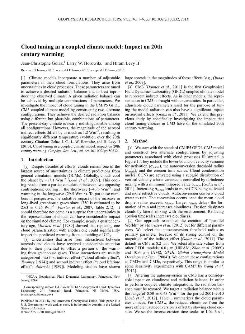
and construct two alternate configurations by adjustingparameters associated with cloud processes illustrated inFigure 1. They include the lower bound on velocity variancefor activation (�w,min), the autoconversion threshold radius(rthresh), and the erosion time scales. Cloud condensationnuclei (CCN) are activated using a subgrid distribution ofvertical velocity whose variance is controlled by turbulencemixing with a minimum imposed value �w,min [Golaz et al.,2011]. Increasing �w,min leads to more CCN being activatedand more reflective clouds. Autoconversion converts cloudwater to rain. The conversion occurs once the mean clouddroplet radius exceeds rthresh. Larger rthresh delays the for-mation of rain and increases cloudiness. Erosion dissipatesclouds by lateral mixing with the environment. Reducingerosion timescales increases cloudiness.

[6] Our approach resembles the creation of “parallelWorlds” by Mauritsen et al. [2012] but for different param-eters. We select the autoconversion threshold radius asprimary parameter because of its strong control on themagnitude of the indirect effect [Golaz et al., 2011]. Thedefault in CM3 is 8.2 �m. We select alternate values fromother GFDL models: 6.0 �m (HiRAM; Zhao et al. [2009])and 10.6 �m (AM2; GFDL Global Atmosphere ModelDevelopment Team [2004]). We denote these configurationsas CM3w and CM3c, respectively. This range is similar tosome sensitivity experiments with CAM5 by Wang et al.[2012].

[7] Altering the autoconversion in CM3 has a consider-able impact on cloudiness and radiation balance. In orderto perform coupled climate integrations, the radiation bal-ance must be restored. We target a radiation balance withinthe range of 0.50 ˙ 0.43 Wm–2 for the period 2001–2010[Loeb et al., 2012]. Table 1 summarizes the cloud param-eter choices. For CM3w, the reduced cloudiness from themore efficient autoconversion is offset by slowing cloud ero-sion. We set the inverse erosion time scales to 1.0e–6 s–1,

1

GOLAZ ET AL.: CLOUD TUNING AND 20TH CENTURY WARMING

Erosion

Autoconversion

CCN

Activation

rain drops

w > 0

Figure 1. Illustration of key cloud processes withadjustable parameters in the GFDL CM3 model: activationof cloud condensation nuclei (CCN) to form cloud droplets,autoconversion of cloud water to rain, and erosion bylateral mixing.

Table 1. Summary of Model Configurationsa

rthresh Erosion��10–6 s–1

��w,min TOA rad.

(�m) Main Conv. Turb.�ms–1

� �Wm–2�

CM3 8.2 1.3 70.0 70.0 0.7 1.81CM3w 6.0 1.0 1.0 1.0 0.7 0.73CM3c 10.6 1.3 70.0 70.0 0.2 0.61

aAdjusted cloud parameters include autoconversion threshold (rthresh),erosion inverse time scales (main value and enhanced values under con-vective and turbulent conditions), and lower bound on the variance foractivation (�w,min). Also listed is the top-of-atmosphere net radiation for theperiod 2001–2010 using fixed sea surface temperature (HadISST; Rayneret al. [2003]).

corresponding to the original value suggested by Tiedtke[1993]. For CM3c, the increased cloudiness from the lessefficient autoconversion is offset by reducing the lowerbound on the variance for activation from 0.7 to 0.2 ms–1.

[8] There is a long history of using autoconversion totune climate models [e.g., Rotstayn, 2000]. Values as lowas 4.5 �m have been reported, even though they arenot supported by observations [e.g., Gerber, 1996; Boerset al., 2006]. Pawlowska and Brenguier [2003] analyzedflight segments whose lengths were comparable to GCMgrid box sizes and found that precipitation in stratocu-mulus clouds forms when the maximum mean volumedroplet radius exceeds 10 �m. Attempts to explain reducedvalues in large-scale models have invoked the neglect ofin-cloud subgrid-scale variability [Pincus and Klein, 2000;Larson et al., 2001] and the dispersion effect [Rotstayn andLiu, 2005].

[9] The tuning choices made here are justifiable based onthe current state-of-the-art. However, some choices might bemore desirable than others. CM3c is the configuration withthe preferable autoconversion setting. In CM3, the lowerbound on the vertical velocity variance for CCN activationis larger than in other studies (e.g., 0.2 m s–1 in Ghan et al.[2001] and 0.3 m s–1 in Storelvmo et al. [2006]). Further-more, the frequency of occurrence of this lower bound is98% [Golaz et al., 2011]. It could be argued that the reducedvalue of 0.2 m s–1 in CM3c is preferable. Erosion timescales are poorly constrained, and both CM3c and CM3ware equally plausible.

3. Results3.1. Atmosphere-only Experiments

[10] We first discuss results from a set of atmosphere-only experiments with climatological boundary conditions.For each configuration, we perform three integrations usingpresent-day SSTs but different forcings: (1) PD: present-day emissions (primary aerosols and short-lived gases)and long-lived greenhouse gas (GHG) concentrations,(2) PI: preindustrial emissions and GHG concentrations,(3) PInonGHG: preindustrial emissions and present-day GHGconcentrations. All three integrations use dynamic poten-tial vegetation (no anthropogenic landuse effect) and neglectforcing from explosive volcanoes. This set of integrationsallows us to calculate the adjusted radiative forcing (AF)with relatively inexpensive simulations (15 years followinga 1 year spin-up in our case).

[11] We compute the total adjusted forcing (AFtot) and thenon-GHG forcing (AFnonGHG). We also estimate the GHGforcing as a residual of the two (AFGHG = AFtot – AFnonGHG).By construction, AFtot incorporates fast responses to allanthropogenic forcings, whereas AFnonGHG isolates effectsof aerosols (direct and indirect), and short-lived gases. Wealso compute the Cess climate sensitivity (�) by uniformlyincreasing SSTs by 2 K [Cess et al., 1989]:

� =�TSST

�F, (1)

where �F is the difference in net top-of-the-atmosphereradiation flux. We define the temperature change metric,� QT � AFtot � �. � QT can be regarded as a first-order corre-late of the possible temperature change from preindustrial topresent-day conditions.

[12] Table 2 lists values of adjusted forcings, Cess sen-sitivity, and temperature change metric. These results con-firm the previous finding that the autoconversion thresholdstrongly modulates the magnitude of the aerosol indirecteffects [Golaz et al., 2011]. In CM3c, autoconversion is theleast efficient, and the indirect effects offset the majorityof the radiative impact from greenhouse gases with a totalAF of 0.34 Wm–2. In CM3w, autoconversion is the mostefficient. The magnitude of the indirect effect is substan-tially reduced, resulting in a total AF of 1.54 Wm–2. Sincethe Cess sensitivity is unaffected, we expect the predictedwarming from preindustrial to present-day to be dominatedby changes in AF.

3.2. Coupled Experiments[13] We perform coupled integrations for CM3w and

CM3c starting from the initial conditions of the first CMIP5CM3 historical ensemble member. Control simulations arefirst run for 100 years to let the shorter time scales in thesystem adjust to the modified cloud tunings. We then create

Table 2. Summary of Adjusted Radiative Forcings (Total, Non-GHG, GHG), Cess Climate Sensitivity �, and Temperature ChangeMetric � QT � AFtot � �.

AFtot AFnonGHG AFGHG � �QTW m–2 W m–2 W m–2 K/

�W m–2� K

CM3 0.99 –1.60 2.59 0.67 0.67CM3w 1.54 –1.01 2.55 0.65 1.00CM3c 0.34 –2.28 2.62 0.66 0.22

2


an ensemble of five historical members (1860–2005) start-ing every 50 years from the control simulations. The controlsimulations are each run for 500 years. All forcings for thecontrol and historical simulations are identical to the CMIP5CM3 integrations. The set of CM3w and CM3c simulationsrepresent a total of nearly 2500 years.

[14] A summary of the present-day (1981–2000) globalmean climatology performance is presented in Figure 2

in the form of target diagrams. The left panel measuresthe performance of the three model configurations againstobservations. For each metric, models tend to be clusteredtogether. The right panel measures the difference betweenalternate configurations CM3c, CM3w, and the referenceCM3. Comparing the two panels, it is clear that the distancebetween models is much smaller than the distance betweenmodels and observations. In other words, the overall impact

Figure 2. Target diagrams [Jolliff et al., 2009] illustrating present-day coupled model performance. Model results areannual mean ensemble averages for the period 1981–2000. Vertical axes represent normalized biases (B*), and horizontalaxes normalized unbiased root mean square difference multiplied by the sign of the model and reference standard deviationdifference (RMSD*0). The left panel compares model with observations, and the right one alternate configurations (CM3c,CM3w) with CM3. Fields shown are sea-level pressure (SLP), 500 hPa geopotential height (z500), 200 and 850 hPazonal wind (U200, U850), sea surface temperature (SST), land air surface temperature (TAS), precipitation (Precip), andshortwave and longwave cloud forcing (SWCF, LWCF). Respective data sources are ERA40, HadISST, CRU, and CERES-EBAF [Uppala et al., 2005; Rayner et al., 2003; Brohan et al., 2006; Loeb et al., 2009].

Figure 3. Time evolution of global mean surface air temperature anomalies. Color lines represent the CMIP5 GFDL CM3model (green) and the two alternate configurations, CM3w (red) and CM3c (blue). Each line is a five-member ensembleaverage. Anomalies are computed with respect to 1881–1920. Model drift is removed by subtracting from each ensemblemember the linear trend of the corresponding period in the control simulation. Also shown are observations from NOAANCDC [Vose et al., 2012], NASA GISS [Hansen et al., 2010], and HadCRUT3 [Brohan et al., 2006]. A 5 year run-ning mean is applied to model results and observations. Letters above the horizontal axis mark major volcanic eruptions:Krakatoa (K), Santa María (M), Agung (A), El Chichón (C), and Pinatubo (P).

3


of the alternate cloud tuning is small when measured againstpresent-day climatology.

[15] However, there is a substantial difference in the tem-poral evolution from preindustrial to present-day as illus-trated in Figure 3 by global mean surface air temperatureanomalies. CM3 tends to underpredict the warming due toa strong cooling from aerosol effects [Donner et al., 2011;Levy et al., 2013]. CM3w (largest AFtot, weakest indirecteffect) is warmer than CM3 and follows observations moreclosely. CM3c (smallest AFtot, strongest indirect effects) iscolder than CM3 with almost no discernible warming excepttowards the end of the simulated period. The spread betweenCM3w and CM3c maximizes during the second half of the20th century when indirect effects are largest because sulfateemissions reach their peak.

[16] The CM3 temperature increases by 0.22°C between1881–1920 and 1981–2000. This number includes a correc-tion for control simulation drift and as a result is smallerthan the 0.32°C warming reported by Donner et al. [2011].For the alternate configurations, the temperature change is0.57°C for CM3w and –0.01°C for CM3c. CM3w is closestto observations, which report warmings of 0.59°C (NOAANCDC), 0.53°C (NASA GISS), and 0.56°C (HadCRUT3).

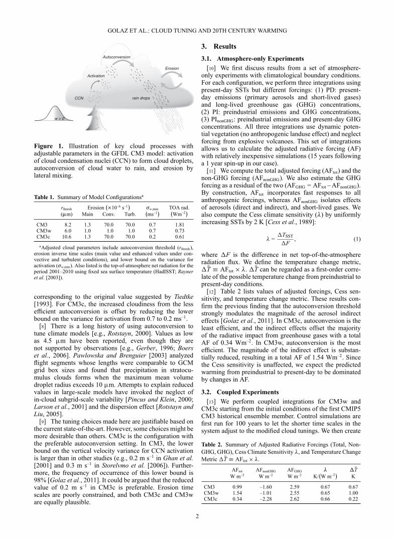
[17] Figure 4 depicts the time evolution of the 700 mocean heat content anomalies. CM3w warms the most andbetter matches observations. Furthermore, it is the only con-figuration with a net preindustrial to present-day increase inocean heat content.

[18] Volcanic eruptions are clearly noticeable in Figures 3and 4. Explosive volcanoes do not impact aerosol con-

centrations in CM3. Instead, an identical times series ofvolcanic optical properties is imposed in all configurations[Donner et al., 2011]. However, the response to individualvolcanoes appears to be generally larger in CM3c thanCM3w. A detailed analysis of the volcanic response isbeyond the scope of this work.

4. Discussion[19] We have shown that there is sufficient ambiguity

in the CM3 adjustable cloud parameters to construct alter-nate configurations (CM3w, CM3c) that achieve the desiredradiation balance. These configurations exhibit only mod-est differences in their present-day climatology. Indeed, onewould be hard pressed to select the “better” configura-tion solely based on present-day metrics such as those inFigure 2. However, CM3w and CM3c differ significantly inthe magnitude of their indirect effects. As a result, their pre-dictions of the 20th century warming are strongly affected(Figures 3 and 4).

[20] CM3w predicts the most realistic 20th century warm-ing. However, this is achieved with a small and lessdesirable threshold radius of 6.0 �m for the onset of pre-cipitation. Conversely, CM3c uses a more desirable valueof 10.6 �m but produces a very unrealistic 20th centurytemperature evolution. This might indicate the presence ofcompensating model errors. Recent advances in the useof satellite observations to evaluate warm rain processes[Suzuki et al., 2011; Wang et al., 2012] might help under-stand the nature of these compensating errors.

Figure 4. Time evolution of global mean upper 700 m ocean heat content anomaly. Color lines repre-sent the CMIP5 GFDL CM3 model (green) and the two alternate configurations, CM3w (red) and CM3c(blue). Each line is a five-member ensemble average. Anomalies are computed with respect to 1860–1880.Model drift is removed by subtracting from each ensemble member the linear trend of the correspond-ing period in the control simulation. Observations from [Levitus, 2012] are shown with offsets to matchmodel averages over the period (1955–2005). Letters above the horizontal axis mark major volcanic eruptions:Krakatoa (K), Santa María (M), Agung (A), El Chichón (C), and Pinatubo (P).

4


[21] CM3 was not explicitly tuned to match the 20thtemperature record. However, our findings indicate thatuncertainties in cloud processes permit a large range ofsolutions for the predicted warming. We do not believethis to be a peculiarity of the CM3 model. Indeed, numer-ous previous studies have documented a strong sensitivityof the radiative forcing from aerosol indirect effects todetails of warm rain cloud processes [e.g., Rotstayn,2000; Menon et al., 2002; Posselt and Lohmann, 2009;Wang et al., 2012]. Furthermore, in order to predicta realistic evolution of the 20th century, models mustbalance radiative forcing and climate sensitivity, resultingin a well-documented inverse correlation between forcingand sensitivity [Schwartz et al., 2007; Kiehl, 2007; Andrewset al., 2012]. This inverse correlation is consistent with anintercomparison-driven model selection process in which“climate models’ ability to simulate the 20th century tem-perature increase with fidelity has become something of ashow-stopper as a model unable to reproduce the 20th cen-tury would probably not see publication” [Mauritsen et al.,2012].

[22] Acknowledgments. We are grateful to Leo Donner and the entireGlobal Atmospheric Model Development Team for innumerable stimulat-ing discussions about AM3/CM3. We acknowledge Tom Delworth andRong Zhang for a thought provoking analysis of CM3 results. Figure 1 wasdrafted by Cathy Raphael.

ReferencesAlbrecht, B. A. (1989), Aerosols, cloud microphysics, and frac-

tional cloudiness, Science, 245, 1227–1230, doi:10.1126/science.245.4923.1227.

Andrews, T., J. M. Gregory, M. J. Webb, and K. E. Taylor (2012), Forcing,feedbacks and climate sensitivity in CMIP5 coupled atmosphere-oceanclimate models, Geophys. Res. Lett., 39, L09712, doi:10.1029/2012GL051607.

Boers, R., J. B. Jensen, P. B. Krummel, and H. Gerber (2006), Micro-physical and short-wave radiative structure of wintertime stratocumulusclouds over the Southern Ocean, Quart. J. Roy. Meteor. Soc., 122(534),1307–1339, doi:10.1002/qj.49712253405.

Brohan, P., J. J. Kennedy, I. Harris, S. F. B. Tett, and P. D. Jones(2006), Uncertainty estimates in regional and global observed tempera-ture changes: A new dataset from 1850, J. Geophys. Res., 111, D12106,doi:10.1029/2005JD006548.

Cess, R. D., et al. (1989), Interpretation of cloud-climate feedback as pro-duced by 14 atmospheric general circulation models, Science, 245(4917),513–516, doi:10.1126/science.245.4917.513.

Donner, L. J., et al. (2011), The dynamical core, physical parameterizations,and basic simulation characteristics of the atmospheric component AM3of the GFDL Global Coupled Model CM3, J. Climate, 24, 3484–3519,doi:10.1175/2011JCLI3955.1.

Forster, P., et al. (2007), Changes in atmospheric constituents and radia-tive forcing, in Climate Change 2007: Contribution of Working Group Ito the Fourth Assessment Report of the Intergovernmental Panel on Cli-mate Change, edited by S. Solomon, et al., Cambridge University Press,New York, 129–234.

Gerber, H. (1996), Microphysics of marine stratocumulus clouds withtwo drizzle modes, J. Atmos. Sci., 53, 1649–1662, doi:10.1175/1520-0469(1996)053<1649:MOMSCW>2.0.CO;2.

GFDL Global Atmosphere Model Development Team (2004), The newGFDL global atmosphere and land model AM2-LM2: Evaluationwith prescribed SST simulations, J. Climate, 17, 4641–4673, doi:10.1175/JCLI-3223.1.

Ghan, S. J., R. C. Easter, J. Hudson, and F.-M. Bréon (2001), Evalua-tion of aerosol indirect radiative forcing in MIRAGE, J. Geophys. Res.,106(D6), 5317–5334, doi:10.1029/2000JD900501.

Golaz, J.-C., M. Salzmann, L. J. Donner, L. W. Horowitz, Y. Ming,and M. Zhao (2011), Sensitivity of the aerosol indirect effect to sub-grid variability in the cloud parameterization of the GFDL Atmosphere

General Circulation Model AM3, J. Climate, 24, 3145–3160, doi:10.1175/2010JCLI3945.1.

Hansen, J., R. Ruedy, M. Sato, and K. Lo (2010), Global sur-face temperature change, Rev. Geophys., 48, RG4004, doi: 10.1029/2010RG000345.

Jolliff, J. K., J. C. Kindle, I. Shulman, B. Penta, M. A. M. Friedrichs,R. Helber, and R. A. Arnone (2009), Summary diagrams for coupledhydrodynamic-ecosystem model skill assessment, J. Mar. Sys., 76,64–82, doi:10.1016/j.jmarsys.2008.05.014.

Kiehl, J. (2007), Twentieth century climate model response andclimate sensitivity, Geophys. Res. Lett., 34, L22710, doi:10.1029/2007GL031383.

Larson, V. E., R. Wood, P. R. Field, J.-C. Golaz, T. H. Vonder Haar,and W. R. Cotton (2001), Systematic biases in the microphysicsand thermodynamics of numerical models that ignore subgrid-scalevariability, J. Atmos. Sci., 58 (9), 1117–1128, doi: 10.1175/1520-0469(2001)058<1117:SBITMA>2.0.CO;2.

Levitus, S., et al. (2012), World ocean heat content and thermosteric sealevel change (0–2000 m), 1955–2010, Geophys. Res. Lett., 39, L10603,doi:10.1029/2012GL051106.

Levy II, H., L. W. Horowitz, D. M. Schwarzkopf, Y. Ming, J.-C. Golaz,V. Naik, and V. Ramaswamy (2013), The roles of aerosol direct andindirect effects in past and future climate change, J. Geophys. Res., inpress, doi:10.1002/jgrd.50192.

Loeb, N. G., B. A. Wielicki, D. R. Doelling, G. L. Smith, D. F. Keyes,S. Kato, N. Manalo-Smith, and T. Wong (2009), Toward optimal clo-sure of the Earth’s top-of-atmosphere radiation budget, J. Climate, 22,748–766, doi:10.1175/2008JCLI2637.1.

Loeb, N. G., J. M. Lyman, G. C. Johnson, R. P. Allan, D. R. Doelling,T. Wong, B. J. Soden, and G. L. Stephens (2012), Observedchanges in top-of-the-atmosphere radiation and upper-ocean heatingconsistent within uncertainty, Nat. Geosci., 5, 110–113, doi:10.1038/NGEO1375.

Mauritsen, T., et al. (2012), Tuning the climate of a global model, J. Adv.Model. Earth Syst., 4, M00A01, doi:10.1029/2012MS000154.

Menon, S., A. D. Del. Genio, D. Koch, and G. Tselioudis (2002),GCM simulations of the aerosol indirect effect: Sensitivity to cloudparameterization and aerosol burden, J. Atmos. Sci., 59, 692–713, doi:10.1175/1520-0469(2002)059<0692:GSOTAI>2.0.CO;2.

Mitchell, J. F. B., C. A. Senior, and W. J. Ingram (1989), CO2 andclimate: A missing feedback? Nature, 341, 132–134, doi: 10.1038/341132a0.

Pawlowska, H., and J.-L. Brenguier (2003), An observational study ofdrizzle formation in stratocumulus clouds for general circulation model(GCM) parameterizations, J. Geophys. Res, 108 (D15), 8630, 13, doi:10.1029/2002JD002679.

Pincus, R., and S. A. Klein (2000), Unresolved spatial variability andmicrophysical process rates in large-scale models, J. Geophys. Res., 105(D22), 27,059–27,065, doi:10.1029/2000JD900504.

Posselt, R., and U. Lohmann (2009), Sensitivity of the total anthropogenicaerosol effect to the treatment of rain in a global climate model, Geophys.Res. Lett., 36, L02805, doi:10.1029/2008GL035796.

Quaas, J., et al. (2009), Aerosol indirect effects—General circulation modelintercomparison and evaluation with satellite data, Atmos. Chem. Phys.,9, 8697–8717, doi:10.5194/acp-9-8697-2009.

Rayner, N. A., D. E. Parker, E. B. Horton, C. K. Folland, L. V. Alexander,D. P. Rowell, E. C. Kent, and A. Kaplan (2003), Global analyses ofsea surface temperature, sea ice, and night marine air temperature sincethe late nineteenth century, J. Geophys. Res., 108 (D14), 4407, doi:10.1029/2002JD002670.

Rotstayn, L. D. (2000), On the “tuning” of autoconversion parameteriza-tions in climate models, J. Geophys. Res., 105(D12), 15,495–15,507, doi:10.1029/2000JD900129.

Rotstayn, L. D., and Y. Liu (2005), A smaller global estimate of thesecond indirect aerosol effect, Geophys. Res. Lett., 32, L05708, doi:10.1029/2004GL021922.

Schwartz, S. E., R. J. Charlson, and H. Rodhe (2007), Quantifying climatechange—Too rosy a picture? Nature Rep. Climate Change, 2, 23–24, doi:10.1038/climate.2007.22.

Storelvmo, T., J. E. Kristjánsson, S. J. Ghan, A. Kirkevåg, Ø. Seland, andT. Iversen (2006), Predicting cloud droplet number concentration inCommunity Atmosphere Model (CAM)-Oslo, J. Geophys. Res., 11,D24208, doi:10.1029/2005JD006300.

Suzuki, K., G. L. Stephens, S. C. van den Heever, and T. Y. Nakajima(2011), Diagnosis of the warm rain process in cloud-resolving mod-els using joint CloudSat and MODIS observations, J. Atmos. Sci., 68,2655–2670, doi:10.1175/JAS-D-10-05026.1.

Tiedtke, M. (1993), Representation of clouds in large-scale models,Mon. Wea. Rev., 121(11), 3040–3061, doi:10.1175/1520-0493(1993)121<3040:ROCILS>2.0.CO;2.

5


Twomey, S. (1974), Pollution and the planetary albedo, Atmos. Environ.,8(12), 1251–1256, doi:10.1016/0004-6981(74)90004-3.

Uppala, S. M., et al. (2005), The ERA-40 re-analysis, Quart. J. Roy. Meteor.Soc., 131, 2961–3012, doi:10.1256/qj.04.176.

Vose, R. S., et al. (2012), NOAA’s merged land-ocean surface tem-perature analysis, Bull. Amer. Meteor. Soc., 93 (11), 1677–1685, doi:10.1175/BAMS-D-11-00241.1.

Wang, M., et al. (2012), Constraining cloud lifetime effects of aerosolsusing A-Train satellite observations, Geophys. Res. Lett., 39, L15709,doi:10.1029/2012GL052204.

Zhao, M., I. M. Held, S.-J. Lin, and G. A. Vecchi (2009), Simulationsof global hurricane climatology, interannual variability, and responseto global warming using a 50-km resolution GCM, J. Climate, 22,6653–6678, doi:10.1175/2009JCLI3049.1.

6

cloud tuning in a coupled climate model: impact on 20th century warming

Documents