HAL Id: hal-01832316https://hal.archives-ouvertes.fr/hal-01832316

Submitted on 7 Jul 2018

HAL is a multi-disciplinary open accessarchive for the deposit and dissemination of sci-entific research documents, whether they are pub-lished or not. The documents may come fromteaching and research institutions in France orabroad, or from public or private research centers.

L’archive ouverte pluridisciplinaire HAL, estdestinée au dépôt et à la diffusion de documentsscientifiques de niveau recherche, publiés ou non,émanant des établissements d’enseignement et derecherche français ou étrangers, des laboratoirespublics ou privés.

Close evaluation of layer potentials in three dimensionsShilpa Khatri, Arnold Kim, Ricardo Cortez, Camille Carvalho

To cite this version:Shilpa Khatri, Arnold Kim, Ricardo Cortez, Camille Carvalho. Close evaluation of layer potentials inthree dimensions. Journal of Computational Physics, 2020, 423, pp.109798. �hal-01832316�

Close evaluation of layer potentials in three dimensions

Camille Carvalho∗ Shilpa Khatri ∗ Arnold D. Kim ∗

July 6, 2018

Abstract

We present a simple and effective method for computing double- and single-layer potentialsfor Laplace’s equation in three dimensions close to the boundary. The close evaluation of theselayer potentials is challenging because they are nearly singular integrals. The method is comprisedof three steps: (i) rotate the spherical coordinate system so that the peak of the kernel in thenearly-singular integral is aligned with its north pole; (ii) integrate first with respect to azimuthusing the Periodic Trapezoid Rule, which is a natural averaging operation yielding a relativelysmooth function of the polar angle; and (iii) integrate with respect to the polar angle (ratherthan the cosine of the polar angle) using an open, Gauss-Legendre quadrature rule mapped to[0, π]. We find that the asymptotic behavior of the error for this method in the limit of smallevaluation distance from the boundary is quadratic for the modified double-layer potential afterapplying a subtraction method to it, and linear for the single-layer potential. Additionally, weuse this method for computing the matrix entries of the Galerkin method to solve the underlyingboundary integral equations. We illustrate the accuracy and utility of this method through severalnumerical examples.

Keywords: Nearly singular integrals, close evaluation problem, potential theory, boundary inte-gral equations, numerical quadrature.

1 Introduction

The close evaluation problem arises in boundary integral methods for numerically solving boundaryvalue problems for linear, elliptic partial differential equations. In boundary integral equation methods,the solution of the boundary value problem is given in terms of double- and single-layer potentials,which are integrals of a kernel multiplied by a density over the boundary of the domain. The kernel forthe single-layer potential is the fundamental solution of the elliptic, partial differential equation and thekernel for the double-layer potential is the normal derivative of that fundamental solution. As a result,each of these kernels has an isolated singularity at a known point on the boundary. When evaluatingdouble- and single-layer potentials at points close to the boundary, the associated kernel is regular,but is sharply peaked because the evaluation point is close to its singular point on the boundary. Forthis reason, we say that double- and single-layer potentials evaluated close to the boundary are nearlysingular integrals.

Nearly singular integrals are more challenging to compute numerically than weakly singular ones.When computing weakly singular integrals, one must explicitly address the singularity in the kernel.For example, weakly singular integrals can be computed accurately using high-order product Nystrommethods [7, 14]. These product Nystrom methods are often used to solve the boundary integralequations for the density. However, for a nearly singular integral, there is no singularity to address.Nonetheless, without effectively addressing the peak in a nearly singular integral, one must increase

∗Applied Mathematics Unit, School of Natural Sciences, University of California, Merced, 5200 North Lake Road,Merced, CA 95343

1

n(y)B

averaging

operation

Figure 1: The point y? on the boundary surface denoted by B, indicated by the outward, unit normal,n(y?). Even though the fundamental solution for Laplace’s equation and its normal derivative aresingular at y?, integration over B includes a natural averaging operation about y? indicated by thedashed closed curve. This averaging operation is important for computing the close evaluation ofdouble- and single-layer potentials in three dimensions.

the order of the quadrature rule to obtain accuracy commensurate with evaluation points that are farfrom the boundary.

The close evaluation problem has been studied extensively. Schwab and Wendland [20] have devel-oped a boundary extraction method based on a Taylor series expansion of the layer potentials. Bealeand Lai [9] have developed a method that first regularizes the nearly singular kernel and then addscorrections for both the discretization and the regularization. The result of this approach is a uniformerror in space. Helsing and Ojala [17] developed a method that combines a globally compensatedquadrature rule and interpolation to achieve very accurate results over all regions of the domain. Bar-nett [8] has used surrogate local expansions with centers placed near, but not on, the boundary. Thiswork led to the work by Klockner et al. [18] that introduces Quadrature By Expansion (QBX). QBXuses expansions about accurate evaluation points far away from the boundary to compute accurateevaluations close to it. The convergence of QBX has been studied in [15]. Moreover, fast implementa-tions of QBX have since been developed [1, 19, 21], and rigorous error estimates have been derived forthe method [2]. Recently, the authors developed a method that involved matched asymptotic expan-sions for the kernel [12]. In that method, the asymptotic expansion that captures the peaked behaviorof the kernel can be integrated exactly and the relatively smooth remainder is integrated numerically,resulting in a highly accurate method.

Most of these aforementioned studies are for two-dimensional problems. There are fewer resultsfor three-dimensional problems. Beale et al. [10] have extended the regularization method to three-dimensional problems. Additionally, QBX has been used for three-dimensional problems [1, 21]. Inprinciple, the matched asymptotic expansion method by the authors can be extended to three dimen-sional problems. However, we do not pursue that approach because the method we present here ismore direct and simpler to implement.

We study the close evaluation of double- and single-layer potentials in the context of the interiorDirichlet and exterior Neumann problems for Laplace’s equation in three dimensions, respectively.Compared to the close evaluation of layer potentials in two dimensions, we find that layer potentials inthree dimensions are actually better behaved because the double integral over the boundary naturallyincludes an averaging operation about y?, the point on the boundary at which the kernels have a sin-gularity (see Fig. 1). This averaging operation is a crucial aspect of the layer potential’s representationof a harmonic function that smoothly approaches its boundary data. To find this inherent averagingoperation, we perform a local analysis of the contribution of the layer potentials in the vicinity of y?.This local analysis provides valuable insight into the close evaluation problem and suggests a natu-ral method for numerically computing nearly singular layer potentials in three dimensions. We alsofind that this method can be used to compute weakly singular integrals, in particular for numericallysolving the boundary integral equation for densities.

2

The remainder of this paper is as follows. We precisely define the close evaluation problem for thedouble- and single-layer potentials in Section 2. In Section 3, we compute the asymptotic behaviorof the contributions to these layer potentials made by a small region containing the point where thekernels are peaked. By doing so, we find a natural numerical method to evaluate these nearly singularintegrals. This numerical method is detailed in Section 4. We discuss in Section 5 how this method canalso be used to compute matrix entries in the Galerkin method to solve the boundary integral equationsfor the densities. We give several examples demonstrating the accuracy of this numerical method inSection 6. Section 7 gives our conclusions. A gives details of how we rotate spherical integrals in theresults presented in this paper, and B gives a useful derivation of the spherical Laplacian.

2 Close evaluation of double- and single-layer potentials

Consider a simply connected, open set denoted by D ⊂ R3 with boundary, B, and let D = D∪B. Forsome given smooth data f , we write the function u ∈ C2(D) ∩ C1(D) satisfying the interior Dirichletproblem,

∆u = 0 in D,

u = f on B,(2.1)

as the double-layer potential,

u(x) =1

4π

∫B

n(y) · (x− y)

|x− y|3µ(y)dσy, x ∈ D, (2.2)

with n(y) denoting the unit, outward normal at y ∈ B, and dσy denoting the surface element. Here,µ is the density for the double-layer potential satisfying

−1

2µ(y?) +

1

4π

∫B

n(y) · (y? − y)

|y? − y|3µ(y)dσy = f(y?), y? ∈ B. (2.3)

Let E = R3\D, and E = E ∪B. Let n still denote the unit normal pointing outward from D. Forsome given smooth data g, we write the function v ∈ C2(E)∩C1(E) satisfying the exterior Neumannproblem,

∆v = 0 in E,

−∂nu = g on B,(2.4)

as the single-layer potential,

v(x) =1

4π

∫B

ρ(y)

|x− y|dσy, x ∈ E. (2.5)

Here, ρ(y) is the density for the single-layer potential satisfying

1

2ρ(y?)− 1

4π

∫B

n(y?) · (y? − y)

|y? − y|3ρ(y)dσy = g(y?), y? ∈ B, (2.6)

Boundary integral equation methods involve solving (2.3) and (2.6) for µ and ρ, respectively. Theseresults are then used to compute u using (2.2) for any desired point in D and v using (2.5) for anydesired point in E. Boundary integral equations (2.3) and (2.6) can be solved to very high accuracyusing Nystrom methods [7, 14]. Thus, the focus turns to accurately computing the double- and single-layer potentials, (2.2) and (2.5), respectively. The high accuracy of Nystrom methods transfers overto the evaluation of these layer potentials except for close evaluation points.

To define a close evaluation point precisely, let 0 < ε� 1 denote a small, dimensionless parameter,and consider

x = y? ∓ ε`n?, (2.7)

3

for x ∈ D and x ∈ E, respectively, with y? ∈ B denoting a point on the boundary, n? = n(y?) denotingthe unit, outward normal from D at y?, and ` denoting a characteristic length of B, e.g. its radius ofcurvature at y?. Before substituting (2.7) into (2.2), we first make use of Gauss’ law [16],

1

4π

∫∂D

n(y) · (x− y)

|x− y|3dσy =

−1 x ∈ D,− 1

2 x ∈ B,0 x ∈ E,

(2.8)

to write the double-layer potential evaluated at the close evaluation point given in (2.7) as

u(y? − ε`n?) = −µ(y?) +1

4π

∫B

n(y) · (y? − y − ε`n?)|y? − y − ε`n?|3

[µ(y)− µ(y?)] dσy. (2.9)

We call (2.9) the modified double-layer potential resulting from applying a subtraction method [14].For the close evaluation of the single-layer potential, we substitute (2.7) into (2.5) and obtain

v(y? + ε`n?) =1

4π

∫B

ρ(y)

|y? − y + ε`n?|dσy. (2.10)

Our objective here is the accurate and efficient numerical evaluation of (2.9) and (2.10). Thechallenge in this problem is that in the asymptotic limit as ε→ 0, those integrals are nearly singular.Setting ε = 0 yields weakly singular integrals which can be numerically evaluated accurately. In fact,this is what is done in the Nystrom method to solve boundary integral equations (2.3) and (2.6).However, when ε is small, but finite, the functions to be integrated are not singular, but they aresharply peaked about y = y? which makes computing (2.9) and (2.10) challenging.

3 Motivation: local analysis of the double- and single-layerpotentials at a close evaluation point

The nearly singular behavior of (2.9) and (2.10) about y = y? is the major cause for error in theirevaluation. For this reason, we analyze the contribution made by a small region about y = y?. Bydoing so, we motivate the method that we use to evaluate (2.9) and (2.10). In general, it is morechallenging to evaluate the double-layer potential than the single-layer potential because the kernelin (2.9) is more peaked than that in (2.10). However, we show below that the modified double-layerpotential given in (2.9) will have a more accurate evaluation than (2.10) due to the subtraction methodthat has been used.

For simplicity, suppose that B is an analytic, closed, and oriented surface. This assumption canbe relaxed to just local smoothness about y? with appropriate technical modifications. We introducethe parameters s ∈ [0, π] and t ∈ [−π, π] for a rotated spherical coordinate system that parametrizesB such that y?/|y?| corresponds to the north pole, i.e. y = y(s, t) and y? = y(0, ·). Details about thisrotated coordinate system can be found in A. In terms of this parameterization, (2.9) is given by

u(y? − ε`n?) = −µ(0, ·) +1

4π

∫ π

−π

∫ π

0

K(s, t; ε) [µ(s, t)− µ(0, ·)] sin(s) dsdt, (3.1)

with µ(s, t) = µ(y(s, t)), µ(0, ·) = µ(y(0, ·)), and

K(s, t; ε) =n(s, t) · (yd(s, t)− ε`n?)|yd(s, t)− ε`n?|3

J(s, t), (3.2)

with n(s, t) = n(y(s, t)), yd(s, t) = y(0, ·)− y(s, t), and J(s, t) = |ys(s, t)× yt(s, t)|/ sin(s). In the limitas ε → 0, this kernel becomes sharply peaked for yd = O(ε) leading to K = O(ε−2). This behaviorcharacterizes this nearly singular integral.

4

We consider the contribution to u made by a small portion of B about y = y?, which we denoteby U . To do so, we introduce the parameter δ > 0 and define

U(y?; ε, δ) =1

4π

∫ π

−π

∫ δ

0

K(s, t; ε) [µ(s, t)− µ(0, ·)] sin(s) dsdt. (3.3)

Next, we substitute s = εS in (3.3), and find

U(y?; ε, δ) =1

4π

∫ π

−π

∫ δ/ε

0

K(εS, t; ε) [µ(εS, t)− µ(0, ·)] sin(εS)εdSdt. (3.4)

Recognizing that n(εS, t) = n? + O(ε), and yd(εS, t) = −εSys(0, ·) + O(ε2) with ys(0, ·) 6= 0 lying onthe plane tangent to B at y?, we find by expanding K(εS, t; ε) about ε = 0 that

K(εS, t; ε) = −`J(0, ·)ε2

1

(S2|ys(0, ·)|2 + `2)3/2+O(ε−1). (3.5)

Substituting this leading-order behavior into (3.4) along with sin(εS) = εS +O(ε3), we obtain

U(y?; ε, δ) = −`J(0, ·)4π

∫ π

−π

∫ δ/ε

0

[S

(S2|ys(0, ·)|2 + `2)3/2+O(ε)

][µ(εS, t)− µ(0, ·)] dSdt. (3.6)

Since the leading-order asymptotic behavior given in (3.5) is independent of t, we use the 2π-periodicityof µ with respect to t to write

U(y?; ε, δ) = −`J(0, ·)4π

∫ δ/ε

0

{[S

(S2|ys(0, ·)|2 + `2)3/2+O(ε)

] [∫ π

0

µ(εS, t) + µ(εS, t− π)− 2µ(0, ·)dt]}

dS.

(3.7)Next, we use the regularity of µ over the north pole to substitute µ(εS, t − π) = µ(−εS, t), and findthat

U(y?; ε, δ) = −`J(0, ·)4π

∫ δ/ε

0

{[S

(S2|ys(0, ·)|2 + `2)3/2+O(ε)

] [∫ π

0

µ(εS, t) + µ(−εS, t)− 2µ(0, ·)dt]}

dS,

= −`J(0, ·)4π

∫ δ/ε

0

{[S

(S2|ys(0, ·)|2 + `2)3/2+O(ε)

] [∫ π

0

ε2S2µss(0, ·) +O(ε4)dt

]}dS,

= −`J(0, ·)4

∫ δ/ε

0

{ε2S3

(S2|ys(0, ·)|2 + `2)3/2

[1

π

∫ π

0

µss(0, ·)dt]}

dS +O(ε2).

(3.8)We find that in the asymptotic limit corresponding to 0 < ε� δ � 1 that∫ δ/ε

0

ε2S3

(S2|ys(0, ·)|2 + `2)3/2dS = δ

ε

|ys(0, ·)|3+O(ε2), (3.9)

(recall that |ys(0, ·)| 6= 0), and in B, we show that

1

π

∫ π

0

µss(0, ·)dt =1

2∆S2µ(y?), (3.10)

with ∆S2µ(y?) denoting the spherical Laplacian of µ evaluated at y?. Thus, we have found that

U(y?; ε, δ) = −δ ε`J(0, ·)8|ys(0, ·)|3

∆S2µ(y?) +O(ε2). (3.11)

This result gives the leading-order asymptotic behavior for U . The results (3.9) and (3.11) provide thefollowing insights about the close evaluation problem.

5

• The function that is integrated in (3.9) has a smooth limit to a finite value at the north pole.In other words, despite the sharply peaked behavior of the kernel, the leading-order asymptoticbehavior of the integrand is smooth.

• Working in a rotated spherical coordinate system in which y?/|y?| serves as the north pole effec-tively removes the dependence with respect to the azimuthal angle, denoted here by t, throughan averaging about the north pole.

• The above procedure provides a way to rewrite the layer potential that avoids the close-evaluationproblem.

Similar conclusions can be drawn for the single-layer potential. Using the same parameterizationas above, we write (2.10) as

v(y? + ε`n?) =1

4π

∫ π

−π

∫ π

0

G(s, t; ε)ρ(s, t) sin(s)dsdt, (3.12)

with ρ(s, t) = ρ(y(s, t)), and

G(s, t; ε) =J(s, t)

|yd(s, t) + ε`n?|. (3.13)

Just as we have done for u, we consider the contribution to v made by a small portion of B abouty = y?, which we denote by V , defined with the parameter δ as

V (y?; ε, δ) =1

4π

∫ π

−π

∫ δ

0

G(s, t; ε)ρ(s, t) sin(s)dsdt. (3.14)

Next, we substitute s = εS and obtain

V (y?; ε, δ) =1

4π

∫ π

−π

∫ δ/ε

0

G(εS, t; ε)ρ(εS, t) sin(εS)εdSdt. (3.15)

By expanding G about ε = 0, we find that that

G(εS, t; ε) =1

ε

J(0, ·)(S2|ys(0, ·)|2 + `2)

1/2+O(1). (3.16)

Substituting this leading-order behavior into (3.15) along with sin(εS) = εS + O(ε3), and ρ(εS, t) =ρ(0, ·) +O(ε), and then integrating that result with respect to t, we obtain

V (y?; ε, δ) =J(0, ·)ρ(0, ·)

2

∫ δ/ε

0

[εS

(S2|ys(0, ·)|2 + `2)1/2

+O(ε2)

]dS. (3.17)

In the asymptotic limit in which 0 < ε� δ � 1, we find that

V (y?; ε, δ) = δJ(0, ·)

2|ys(0, ·)|ρ(0, ·) +O(ε). (3.18)

This result gives the leading-order asymptotic behavior for V .In light of the asymptotic analysis given above, we have found a natural procedure to compute

the close evaluation of layer potentials that avoids the challenges associated with evaluating nearlysingular integrals. There are three, crucial steps in this procedure.

1. Rotate the spherical coordinate system so that y?/|y?| serves as the north pole where y? denotesthe boundary point at which the kernel for the layer potential is peaked.

6

2. Integrate first with respect to the azimuthal angle to average the function about the north pole.

3. Integrate the remaining function with respect to the polar angle.

It is important in the third step to integrate with respect to s rather than z = cos(s), which is oftendone, because the asymptotic analysis above is explicitly aided by sin(s) term inherent in the sphericalintegral.

These results suggest that following these three steps leads to a natural numerical method toevaluate double- and single-layer potentials close to the boundary. The leading-order asymptoticbehaviors given by (3.11) and (3.18) show that this method yields an O(ε2) error for the modifieddouble-layer potential and an O(ε) error for the single-layer potential. The smaller error with themodified double-layer potential is due to the subtraction of µ(y?) in conjunction with the azimuthalaveraging step. Additionally (3.11) and (3.18) provide explicit expressions for the limiting behaviorof the double- and single-layer potentials, respectively, as s → 0. These results may be used in thecomputation of the integral with respect to the polar angle in the third step. However, we avoidneeding these results in the specific method we give below by choosing an open quadrature rule for sthat does not require evaluation at the end points of the interval.

4 Numerical method for the close evaluation of double- andsingle-layer potentials

We now give a numerical method for computing the close evaluation of double- and single-layer po-tentials by following the three-step procedure given above. Suppose we have parameterized B byy = y(θ, ϕ) with θ ∈ [0, π] and ϕ ∈ [−π, π] where y? = y(θ?, ϕ?). We seek to compute

I3D(y?) =1

4π

∫ π

−π

∫ π

0

F (θ, ϕ; θ?, ϕ?) sin(θ) dθdϕ, (4.1)

where F is nearly singular at (θ, ϕ) = (θ?, ϕ?). For the modified double-layer potential resulting fromapplying a subtraction method, we have

F (θ, ϕ; θ?, ϕ?) =n(θ, ϕ) · [y(θ?, ϕ?)− y(θ, ϕ)− ε`n(θ?, ϕ?)]

|y(θ?, ϕ?)− y(θ, ϕ)− ε`n(θ?, ϕ?)|3J(θ, ϕ) [µ(θ, ϕ)− µ(θ?, ϕ?)] , (4.2)

and for the single-layer potential, we have

F (θ, ϕ; θ?, ϕ?) =J(θ, ϕ)

|y(θ?, ϕ?)− y(θ, ϕ) + ε`n(θ?, ϕ?)|ρ(θ, ϕ), (4.3)

where J(θ, ϕ) = |yθ(θ, ϕ)× yϕ(θ, ϕ)|/ sin θ.Motivated by the local analysis leading to (3.11) and (3.18) above, we perform the following three-

step procedure to numerically evaluate I3D(y?).

1. Rotate this integral to another spherical coordinate system whose north pole is aligned withy?/|y?|. The details of this rotation are given in A, and lead to θ = θ(s, t) and ϕ = ϕ(s, t) withs ∈ [0, π] and t ∈ [−π, π] where θ(0, ·) = θ? and ϕ(0, ·) = ϕ?. Upon applying this rotation, weobtain the spherical integral

I3D(y?) =1

4π

∫ π

−π

∫ π

0

F (s, t) sin(s) dsdt, (4.4)

with F (s, t) = F (θ(s, t), ϕ(s, t); θ?, ϕ?).

7

2. Use the 2N -point Periodic Trapezoid Rule to compute

1

2π

∫ π

−πF (s, t)dt = F (s) ≈ FN (s) =

1

2N

2N∑j=1

F (s, tj), (4.5)

with tj = −π + π(j − 1)/N for j = 1, . . . , 2N .

3. Use the N -point Gauss-Legendre quadrature rule to compute the integral in s. Let zi ∈ (−1, 1)for i = 1, · · · , N denote the Gauss-Legendre quadrature points with corresponding weights wi.We map the quadrature points according to si = π(zi + 1)/2 to the interval (0, π) and computethe numerical approximation,

I3D ≈ IN3D =π

4

N∑i=1

FN (si) sin(si)wi. (4.6)

In the first step of the procedure, the coordinate system is rotated so that (θ?, ϕ?) correspondsto the north pole of the spherical coordinate system. This rotation sets up the second step, whichcomputes the azimuthal average of the function with respect to t about the north pole. The factor of1/(2π) is incorporated into this step to explicitly obtain an averaging operation yielding FN (s), whichis a smooth function in the polar angle, s. For the third step, we have chosen to use the Gauss-Legendrequadrature rule for which the quadrature points satisfy 0 < s1 < s2 < · · · < sN < π. Consequently,we do not need to explicitly evaluate FN (0). Alternatively, we could have chosen a closed rule thatincludes the end points. For that case, we would use (3.11) and (3.18) to explicitly prescribe the neededvalues in the limit as s→ 0.

This numerical method is based on the product Gaussian quadrature rule for spherical integrals [3].That quadrature rule uses a 2N -point Periodic Trapezoid Rule in the azimuthal angle and N -pointGauss-Legendre quadrature rule in the cosine of the polar angle, z = cos(s) ∈ [−1, 1]. However,the results of the local analysis above show that integrating with respect to the polar angle, s, isbetter since the factor of sin(s) plays an important role in the asymptotic behavior. Thus, rather thantransforming (4.1) by substituting z = cos(s), we map the Gauss-Legendre quadrature rule from [−1, 1]to [0, π] using si = π(zi + 1)/2 for i = 1, · · · , N . Consequently, the mapped quadrature weights areπwj/2, which is accounted for in (4.6) by the π/4 factor. We show in the numerical results presentedin Section 6 that this subtle and seemingly small change to the product Gaussian quadrature rule issignificant and yields substantially better results.

Provided that the densities, µ and ρ, for the double- and single-layer potentials, respectively, areknown to very high accuracy, the main cause of numerical error for the close evaluation problem is dueto the sharp peak of the kernels about y = y?. For that case, the leading-order asymptotic expansionsgiven by (3.11) and (3.18) indicate that this numerical method yields an O(ε2) error for the modifieddouble-layer potential and an O(ε) error for the single-layer potential, respectively. These asymptoticerror estimates are valid only when the value of N used in this numerical method is sufficiently largeto resolve the density and the boundary. Otherwise, errors introduced by inaccuracy of the densityand/or under-resolution of the boundary will dominate over these asymptotic error estimates.

5 Numerical solution of the boundary integral equations

The numerical method described above can also be used to solve the boundary integral equations forthe densities, (2.3) and (2.6). We describe its use in the context of the Galerkin method [4, 5, 6, 7].As we have done above, we suppose that we have parameterized B by y = y(θ, ϕ) with θ ∈ [0, π] andϕ ∈ [−π, π].

To compute the density, µ, for the double-layer potential, we write (2.3) compactly as

−1

2µ+ KD[µ] = f. (5.1)

8

We introduce the approximation for µ,

µ(y(θ, ϕ)) = µ(θ, ϕ) ≈N−1∑n=0

n∑m=−n

Ynm(θ, ϕ)µnm, (5.2)

with {Ynm(θ, ϕ)} denoting the orthonormal set of spherical harmonics. Note that N in (5.2) cor-responds also to the order of the quadrature rule detailed in Section 4 so that the order of thisapproximation is commensurate with the order of the quadrature rule to be used. Substituting (5.2)into (5.1) and taking the inner product with Yn′m′(θ?, ϕ?), we obtain the Galerkin equations,

−1

2µn′m′ +

N−1∑n=0

n∑m=−n

〈Yn′m′ ,KD[Ynm]〉µnm = 〈Yn′m′ , f〉, (5.3)

with

KD[Ynm](θ?, ϕ?) =1

4π

∫ π

−π

∫ π

0

[n(θ, ϕ) · (y(θ?, ϕ?)− y(θ, ϕ))

|y(θ?, ϕ?)− y(θ, ϕ)|3J(θ, ϕ) sin(θ)

]Ynm(θ, ϕ)dθdϕ. (5.4)

We construct the N2 × N2 linear system for the unknown coefficients, µn′m′ resulting from (5.3)evaluated for n′ = 0, · · · , N − 1 with corresponding values of m′. To evaluate (5.4), we use (2.8) torewrite it as

KD[Ynm](θ?, ϕ?) = −1

2Ynm(θ?, ϕ?)

+1

4π

∫ π

−π

∫ π

0

[n(θ, ϕ) · (y(θ?, ϕ?)− y(θ, ϕ))

|y(θ?, ϕ?)− y(θ, ϕ)|3J(θ, ϕ) sin(θ)

][Ynm(θ, ϕ)− Ynm(θ?, ϕ?)] dθdϕ, (5.5)

and evaluate the integral in this expression using the numerical method described above. To computethe inner products, 〈Yn′m′ ,KD[Ynm]〉 and 〈Yn′m′ , f〉, we use the product Gaussian quadrature rulefor spherical integrals [3] with N Gauss-Legendre quadrature points and 2N Periodic Trapezoid Rulepoints.

To compute the density ρ for the single-layer potential, we write (2.6) compactly as

1

2ρ−KS [ρ] = g. (5.6)

We introduce the approximation for ρ,

ρ(y(θ, ϕ)) = ρ(θ, ϕ) ≈N−1∑n=0

n∑m=−n

Ynm(θ, ϕ)ρnm. (5.7)

Performing the same calculations as above, we find that ρnm satisfies the Galerkin equations,

1

2ρn′m′ −

N−1∑n=0

n∑m=−n

〈K †S [Yn′m′ ], Ynm〉ρnm = 〈Yn′m′ , g〉, (5.8)

where K †S denotes the adjoint of KS defined according to

K †S [Yn′m′ ](θ, ϕ) =

1

4π

∫ π

−π

∫ π

0

[n(θ?, ϕ?) · (y(θ?, ϕ?)− y(θ, ϕ))

|y(θ?, ϕ?)− y(θ, ϕ)|3J(θ?, ϕ?) sin(θ?)

]Yn′m′(θ?, ϕ?)dθ?dϕ?.

(5.9)

9

Recall that n(θ?, ϕ?) is the unit normal pointing out of D. For this integral, we use (2.8) to write

K †S [Yn′m′ ](θ, ϕ) = −1

2Yn′m′(θ, ϕ)

+1

4π

∫ π

−π

∫ π

0

[n(θ?, ϕ?) · (y(θ?, ϕ?)− y(θ, ϕ))

|y(θ?, ϕ?)− y(θ, ϕ)|3J(θ?, ϕ?) sin(θ?)

][Yn′m′(θ?, ϕ?)− Yn′m′(θ, ϕ)] dθ?dϕ?,

(5.10)

which we then compute using the numerical method described above. We use the product Gaussianquadrature rule with N Gauss-Legendre quadrature points and 2N Periodic Trapezoid Rule points tocompute the remaining inner products, 〈K †

S Yn′m′ , Ynm〉 and 〈Yn′m′ , g〉, needed to form the N2 ×N2

linear system for the unknown coefficients, ρn′m′ for n′ = 0, · · · , N −1 and corresponding values of m′.

6 Numerical results

We present numerical results for computing the close evaluation of double- and single-layer potentialsusing the method detailed in Section 4. For the double-layer potential examples discussed in Section6.1 below, we have computed the density, µ, by solving boundary integral equation (5.1) using theGalerkin method discussed in Section 5. Then, we compute the double-layer potential using thatdensity for two ellipsoids and study the error. In Section 6.2 below, we compute the representationformula for a harmonic function given as the difference between the double- and single-layer potentialsusing densities that are known exactly. We study the error in computing this representation formulain two different domains and evaluate those results.

6.1 Double-layer potential

We present results in computing the solution of the interior Dirichlet problem (2.1) for two differentellipsoids. For all of these examples, we set the harmonic function,

uex(x) = |x− x0|−1, x ∈ D, (6.1)

with x0 ∈ E to be the exact solution. Therefore, we prescribe

f(y) = |y − x0|−1, y ∈ B, (6.2)

as the Dirichlet boundary data.With the boundary data given in (6.2), we first use the Galerkin method described in Section 5

to solve for µnm, the expansion coefficients for the density introduced in (5.2). We then use (5.2) toevaluate the density, µ, that is needed for computing the double-layer potential. To test our method forclose evaluation points, we evaluate the double-layer potential at the points x = y?− εn? (we have set` = 1) for various points y? on the boundary of the domain and for various ε. The error is determinedby computing the absolute value of the difference between the double-layer potential result and theexact harmonic function, uex(y?− εn?) = |y?− εn?−x0|−1. We show error results for computing u(x)over a range of ε values spanning several orders of magnitude using four different methods listed belowusing the kernel, K defined in (3.2).

Method 1: Compute

u(y? − εn?) =1

4π

∫ π

−π

∫ 1

−1K(cos−1(z), t; ε)µ(cos−1(z), t)dzdt

using an N -point Gauss-Legendre quadrature rule for z ∈ [−1, 1] and a 2N Periodic TrapezoidRule for t ∈ [−π, π].

10

Method 2: Compute

u(y? − εn?) =1

4π

∫ π

−π

∫ π

0

K(s, t; ε)µ(s, t) sin(s)dsdt

using an N -point Gauss-Legendre quadrature rule for s ∈ [0, π] and a 2N Periodic TrapezoidRule for t ∈ [−π, π].

Method 3: Compute

u(y? − εn?) = −µ(0, ·) +1

4π

∫ π

−π

∫ 1

−1K(cos−1(z), t; ε)

[µ(cos−1(z), t)− µ(0, ·)

]dzdt

using an N -point Gauss-Legendre quadrature rule for z ∈ [−1, 1] and a 2N Periodic TrapezoidRule for t ∈ [−π, π].

Method 4: Compute

u(y? − εn?) = −µ(0, ·) +1

4π

∫ π

−π

∫ π

0

K(s, t; ε) [µ(s, t)− µ(0, ·)] sin(s)dsdt

using an N -point Gauss-Legendre quadrature rule for s ∈ [0, π] and a 2N Periodic TrapezoidRule for t ∈ [−π, π].

For each of these methods, we have applied the rotation of the coordinate system described as thefirst step in the procedure detailed in Section 4. Methods 1 and 2 compute the double-layer potentialgiven by (2.2) directly and integrate with respect to z = cos(s) and s, respectively. Methods 3 and4 use the subtraction method, so they compute the modified double-layer potential given in (2.9).Method 3 integrates with respect to z = cos(s) and Method 4 integrates with respect to s. Method 4is the one we have proposed here to compute the close-evaluation of the double-layer potential.

In the examples that follow, we consider two different ellipsoids used by Atkinson [4]. Let (x1, x2, x3)denote an ordered triple in a Cartesian coordinate system. The boundaries for these ellipsoids are givenby

y(θ, ϕ) = (α sin θ cosϕ, β sin θ sinϕ, γ cos θ), θ ∈ [0, π], ϕ ∈ [−π, π]. (6.3)

For the first example, we set α = 1, β = 1.5, and γ = 2, and for the second example, we set α = 1,β = 2, and γ = 5. These two ellipsoids, which we call Ellipsoids 1 and 2, are shown as the left andright plots in Fig. 2, respectively. For both of these examples, we have set x0 = (5, 4, 3) ∈ E in (6.1)and (6.2). In Fig. 2 we also identify two boundary points, labeled A and B, lying on the x1x3-planeand the x1x2-plane, respectively, which we will refer to below when we discuss the error results. Thecoordinates for these points are A = (−1.16,−0.64, 0) and B = (−0.72, 0, 1.75) for Ellipsoid 1, and A= (−0.74,−0.93, 0) and B = (−1.81, 0, 2.13) for Ellipsoid 2.

We have used the Galerkin method with N = 48 to compute the density, µ. For Ellipsoid 1 shownin the left plot of Fig. 2, we find that this order resolves µ with an estimated truncation error on theorder of 10−15. Ellipsoid 2 shown in the right plot of Fig. 2 is more elongated along the x3 axis, so itdeviates farther from a sphere than Ellipsoid 1. As a result, we find that the Galerkin method withN = 48 yields a larger estimated truncation error for µ on the order of 10−12. We have subsequentlyused N = 48 in the quadrature rules for the four methods given above.

6.1.1 Results for Ellipsoid 1

In the top row of Fig. 3, we plot log10 of the error made using Method 1. The left two plots showthe error over the vertical x1x3-plane and a close-up of the small region near the boundary point, A= (−1.16,−0.64, 0). The right two plots show the error over the horizontal x1x2-plane and a close-up

11

A

B

A

B

Figure 2: (Left) Boundary surface of the ellipsoid given by (6.3) with α = 1, β = 1.5, and γ = 2 whichwe call Ellipsoid 1. (Right) Boundary surface of the ellipsoid given by (6.3) with α = 1, β = 2, andγ = 5, which we call Ellipsoid 2. In each figure, the two black curves indicate where the boundaryof the ellipsoid intersects with the vertical x1x3-plane, and the horizontal x1x2-plane, and the blackarrows give the unit outward normal vectors on those curves. The two boundary points labeled A andB lying on the x1x3-plane and x1x2-plane, respectively, give the locations where we investigate theerror made by four different methods. The coordinates for these points are A = (−1.16,−0.64, 0) andB = (−0.72, 0, 1.75) in the left plot, and A = (−0.74,−0.93, 0) and B = (−1.81, 0, 2.13) in the rightplot.

of the small region near the boundary point, B = (−0.72, 0, 1.75). The bottom row of Fig. 3 shows thesame plots for Method 4.

These results show that using Method 1 leads to an O(1) error close to the boundary which issymptomatic of the close evaluation problem. In contrast, the results using Method 4 show an errorthat is several orders of magnitude smaller. To examine this error more closely, we show in Fig. 4errors using Methods 1, 2, 3, and 4 evaluated along the normal at point A = (−1.16,−0.64, 0) on theboundary and the x1x3-plane, and at point B = (−0.72, 0, 1.75) on the boundary and the x1x2-plane.In this way, we clearly observe that the subtraction method used in Method 3 and Method 4 leads tosubstantially smaller errors compared with those made using Method 1 and Method 2. The error forMethods 1, 2, and 3 all appear to asymptote to a fixed value as ε → 0. In contrast, we see that theerror for Method 4 decreases as ε → 0. To study the asymptotic behavior of the error for Method 4,we compute the best linear fit to the error (see dashed black lines in Fig. 4) for the four smallest εvalues. These linear fits have slopes of 1.73 for point A and 1.83 for point B consistent with the O(ε2)error estimate from the asymptotic analysis in (3.11).

6.1.2 Results for Ellipsoid 2

The error results for Ellipsoid 2 plotted in Figs. 5 and 6 are of the same format as those for Ellipsoid1 in Figs. 3 and 4, respectively. The close-ups in Fig. 5 show small regions near the boundary pointsA = (−0.74,−0.93, 0) and B = (−1.81, 0, 2.13).

Figure 5 shows that the error for Method 4 is again several orders of magnitude smaller than thatfor Method 1. However, the magnitude of the errors appears to be larger for both methods than theprevious example. This is due to the larger truncation error associated with the Galerkin method.

12

A

B

A

B

A

B

Method 1

Method 4

Figure 3: The errors made by Method 1 (top row) and Method 4 (bottom row) for Ellipsoid 1. Thefirst and second columns show log10 of the errors made by these two methods in the x1x3-plane, withthe plots in the second column showing a close-up in the vicinity of point A = (−1.16,−0.64, 0). Thethird and fourth columns show log10 of the errors made by these two methods in the x1x2-plane, withthe plots in the fourth column showing a close-up in the vicinity of point B = (−0.72, 0, 1.75).

Figure 4: Comparison of errors made by Methods 1 – 4 for Ellipsoid 1 for evaluation points along thenormal at distance ε from point A = (−1.16,−0.64, 0) on the boundary and in the x1x3-plane (leftplot) and for evaluation points along the normal at distance ε from point B = (−0.72, 0, 1.75) on theboundary and in the x1x2-plane (right plot). The dashed black lines show the best linear fit throughthe Method 4 errors for the four smallest ε values. Both fits are consistent with the O(ε2) asymptoticerror estimate given by (3.11).

In Fig. 6, we see that Method 4 clearly has the smallest error. The dashed black lines show the bestlinear fit to the errors for the four smallest ε values. These linear fits have slopes of 1.83 for point Aand 1.92 for point B consistent with O(ε2) error estimate in (3.11).

13

A

A

B

A

B

B

Method 1

Method 4

Figure 5: The errors made by Method 1 (top row) and Method 4 (bottom row) for Ellipsoid 2. Thefirst and second columns show log10 of the errors made by these two methods in the x1x3-plane withthe plots in the second column showing a close-up in the vicinity of point A = (−0.74,−0.93, 0). Thethird and fourth columns show log10 of the errors made by these two methods in the x1x2-plane withthe plots in the fourth column showing a close-up in the vicinity of point B = (−1.81, 0, 2.13).

Figure 6: Comparison of errors made by Methods 1 – 4 for Ellipsoid 2 for evaluation points along thenormal at distance ε from point A = (−0.74,−0.93, 0) on the boundary and in the x1x3-plane (leftplot) and for evaluation points along the normal at distance ε from point B = (−1.81, 0, 2.13) on theboundary and in the x1x2-plane (right plot). The dashed, black lines show the best linear fit throughthe Method 4 errors for the four smallest ε values. Both fits are consistent with the O(ε2) asymptoticerror estimate given by (3.11).

14

6.1.3 Summary of double-layer potential results

For both Ellipsoids 1 and 2, we have observed that Method 4 provides the most accurate evaluation ofthe double-layer potential for close evaluation points. Method 3 is the next most accurate. However,the errors for Methods 1, 2, and 3 all appear to asymptote to a finite value rather than decay to zeroas the error for Method 4 does. For this reason, we conclude that Method 4 is an effective method forthe close evaluation of the double-layer potential.

The errors for Method 4 plotted in Figs. 4 and 6 show a characteristic behavior. For very smallvalues of ε corresponding to points very close to the boundary, Method 4 is highly accurate with anerror approaching machine precision. For intermediate values of ε, the error obtained with Method4 increases as the value of ε starts to coincide with the spacing of the Gauss-Legendre quadraturepoints in the polar angle s. For bigger values of ε, Methods 1, 2, 3, and 4 have errors of a similarorder of magnitude because the evaluation point is far enough from the boundary that the double-layerpotential is no longer nearly singular.

6.2 The representation formula

When the truncation error for the Galerkin method is not sufficiently small, it dominates over theasymptotic error for the close evaluation of the double-layer potential given by (3.11) and the single-layer potential given by (3.18). For the exterior Neumann problem, (2.4), boundary data are in termsof the gradient of a harmonic function. Consequently, those boundary data tend to be less smooththan those for the interior Dirichlet problem. Because of this, the Galerkin method to solve boundaryintegral equation (5.6) for a boundary that deviates significantly from a sphere requires N in (5.7) to besufficiently large that the truncation error does not interfere with the O(ε) asymptotic error estimatefor the single-layer potential. It is in this way that the Galerkin method is a limitation and anotherhigh-order method can be used to compute the densities for the double- and single-layer potentials formore general domains [11].

The focus of this paper is in the close evaluation problem. Thus, we consider an alternate exampleto test the asymptotic error estimates for the double- and single-layer potentials rather than consideranother high-order method to solve weakly singular boundary integral equations for the densities.Consider the representation formula for a harmonic function in domain D with boundary B,

u(x) =1

4π

∫B

[1

|x− y|n(y) · ∇u(y)− n(y) · (x− y)

|x− y|3u(y)

]dσy, x ∈ D. (6.4)

Given a prescribed harmonic function u and its normal derivative on B, (6.4) gives a formula forcomputing u(x) for any x ∈ D in terms of the difference between the single- and double-layer potentials,where the prescribed boundary data can be interpreted as the corresponding densities, ρ and µ. Forthis case there is no boundary integral equation to solve since the densities are known exactly.

For the following examples, we have set the harmonic function

uex(x1, x2, x3) = ex3(sinx1 + sinx2), (6.5)

following Beale et al. [10], to be the exact solution. We set (6.5) on the boundary to be µ and itsnormal derivative on the boundary to be ρ, which are used in the double- and single-layer potentials,respectively, to evaluate (6.4). For the following examples, we use the four methods described below.

Method 1: Compute

u(y? − εn?) =1

4π

∫ π

−π

∫ 1

−1

[G(cos−1(z), t; ε)ρ(cos−1(z), t)−K(cos−1(z), t; ε)µ(cos−1(z), t)

]dzdt

using an N -point Gauss-Legendre quadrature rule for z ∈ [−1, 1], and a 2N Periodic TrapezoidRule for t ∈ [−π, π].

15

Method 2: Compute

u(y? − εn?) =1

4π

∫ π

−π

∫ π

0

[G(s, t; ε)ρ(s, t)−K(s, t; ε)µ(s, t)] sin(s)dsdt

using an N -point Gauss-Legendre quadrature rule for s ∈ [0, π], and a 2N Periodic TrapezoidRule for t ∈ [−π, π].

Method 3: Compute

u(y?−εn?) = µ(0, ·)+ 1

4π

∫ π

−π

∫ 1

−1

[G(s, t; ε)ρ(cos−1(z), t)−K(cos−1(z), t; ε)

[µ(cos−1(z), t)− µ(0, ·)

]]dzdt

using an N -point Gauss-Legendre quadrature rule for z ∈ [−1, 1], and a 2N Periodic TrapezoidRule for t ∈ [−π, π].

Method 4: Compute

u(y? − εn?) = µ(0, ·) +1

4π

∫ π

−π

∫ π

0

[G(s, t; ε)ρ(s, t)−K(s, t; ε) [µ(s, t)− µ(0, ·)]] sin(s)dsdt

using an N -point Gauss-Legendre quadrature rule for s ∈ [0, π], and a 2N Periodic TrapezoidRule for t ∈ [−π, π].

Here, K is the kernel defined in (3.2) and G is the kernel defined in (3.13).Those four methods are a combination of the four methods used in Section 6.1 for the double-layer

potential, and the corresponding evaluation of the single-layer potential. Methods 1 and 2 do notuse the subtraction method for the double-layer potential, and Methods 3 and 4 use the subtractionmethod. Methods 1 and 3 integrate with respect to z = cos(s), and Methods 2 and 4 integrate withrespect to s. According to the asymptotic error estimates given by (3.11) and (3.18), we expect Method4 to exhibit an O(ε) error in evaluating (6.4).

A

BA

B

Figure 7: (Left) Boundary surface of the peanut-shaped domain given by (6.6) with R(θ) given by(6.7). (Right) Boundary surface of the inverted mushroom cap domain given by (6.6) with R(θ) givenby (6.8). In both domains, the two black curves indicate where the boundary intersects with thevertical x1x3-plane, and the horizontal x1x2-plane, and the black arrows give the unit outward normalvectors on those curves. The two boundary points labeled A and B lying on the x1x3-plane and x1x2-plane, respectively, give the locations where we investigate the error made by four different methods.For the peanut-shaped domain, A = (−0.16,−0.21, 0) and B = (−1.04, 0, 0.94), and for the invertedmushroom cap, A = (−3.07,−1.27, 0) and B = (−1.55, 0, 1.41).

16

In the examples that follow, we consider two domains used by Atkinson [4, 5]. The boundaries forthese two domains are given by

y(θ, ϕ) = R(θ)(sin θ cosϕ, 2 sin θ sinϕ, cos θ), θ ∈ [0, π], ϕ ∈ [−π, π]. (6.6)

For the first example, which resembles a peanut, we have set

R(θ) =

√cos 2θ +

√1.1− sin2 2θ. (6.7)

For the second example, which resembles an inverted mushroom cap, we have set

R(θ) = 2− 1

1 + 100(1− cos θ). (6.8)

The peanut and inverted mushroom cap domains are shown as the left and right plots in Fig. 7,respectively. In Fig. 7, we identify two boundary points, labeled A and B, lying on the x1x3-planeand the x1x2-plane, respectively. For the peanut, A = (−0.16,−0.21, 0) and B = (−1.04, 0, 0.94). Forthe inverted mushroom cap, A = (−3.07,−1.27, 0) and B = (−1.55, 0, 1.41). We refer to these pointsbelow when we discuss the error results.

Since we use exact densities, we are more easily able to use highly resolved computations for thesetwo examples. For the peanut domain, we have set N = 120 and for the inverted mushroom cap, wehave set N = 80.

6.2.1 Results for peanut-shaped domain

The error results plotted in Figs. 8 and 9 are the same format as those in Figs. 3 and 4, respectively.Just like those for the double-layer potential, the results in Fig. 8 clearly show that the error for Method4 is several orders of magnitude smaller than that for Method 1. Moreover, Fig. 9 shows that Methods3 and 4 have significantly smaller errors than Methods 1 and 2 demonstrating that using the modifieddouble-layer potential resulting from applying the subtraction method is effective. These errors showthat Methods 1, 2, and 3 asymptote to a fixed value as ε → 0. In contrast, the error for Method 4decreases as ε→ 0. To study the asymptotic behavior of the error for Method 4, we compute the bestlinear fit to the error (see dashed black lines in Fig. 9) for the four smallest ε values along the normalfor two chosen points, A and B. These linear fits have slopes of 1.00 for point A and 1.01 for point Bconsistent with the expected O(ε) error estimate.

6.2.2 Results for inverted mushroom cap domain

The error results plotted in Figs. 10 and 11 are the same format as those in Figs. 8 and 9, respectively.Fig. 10 also shows that Method 4 clearly outperforms Method 1. Fig. 11 shows that the subtractionmethod used for Methods 3 and 4 yields much better results compared with those for Methods 1 and2. Again, Methods 1, 2, and 3 all appear to asymptote to a fixed value as ε → 0, where Method 4decreases. The dashed black lines in Fig. 11 show the best linear fits to the error for Method 4 forthe four smallest ε values. The slopes of these linear fits are 1.01 for point A and 1.00 for point Bconsistent with the expected O(ε) error estimate given by (3.18).

6.2.3 Summary of representation formula results

For both the peanut and inverted mushroom cap domains, we have observed that Method 4 providesthe most accurate evaluation of the representation formula for close evaluation points. Method 3 is thenext most accurate due to the use of the subtraction method. The errors of Methods 1, 2, and 3 allasymptote to a finite value as ε→ 0, whereas the error for Method 4 decays to zero as O(ε). For thisreason, we conclude that Method 4 is effective for the close evaluation of the representation formula.The error for Method 4 demonstrates the same characteristic behavior discussed for the double-layer

17

A

B

A

B

A

B

Method 1

Method 4

Figure 8: The errors made by Method 1 (top row) and Method 4 (bottom row) for the peanut-shapeddomain shown on the left plot of Fig. 8. The first and second columns show log10 of the errors madeby these two methods in the x1x3-plane with the plots in the second column showing a close-up in thevicinity of point A = (−0.16,−0.21, 0). The third and fourth columns show log10 of the errors madeby these two methods in the x1x2-plane with the plots in the fourth column showing a close-up in thevicinity of point B = (−1.04, 0, 0.94).

Figure 9: Comparison of errors made by Methods 1 – 4 for the peanut-shaped domain for evaluationpoints along the normal at distance ε from point A = (−0.16,−0.21, 0) on the boundary and inthe x1x3-plane (left plot) and for evaluation points along the normal at distance ε from point B= (−1.04, 0, 0.94).on the boundary and in the x1x2-plane (right plot). The dashed, black lines showthe best linear fit through the Method 4 errors for the four smallest ε values. For both fits, the slopesare consistent with the O(ε) asymptotic error estimate.

potential. Namely, for very small values of ε, the error is O(ε). For intermediate values of ε, the errorincreases as the value of ε coincides with the spacing of the Gauss-Legendre quadrature points in the

18

A

B

A

B

A

B

Method 1

Method 4

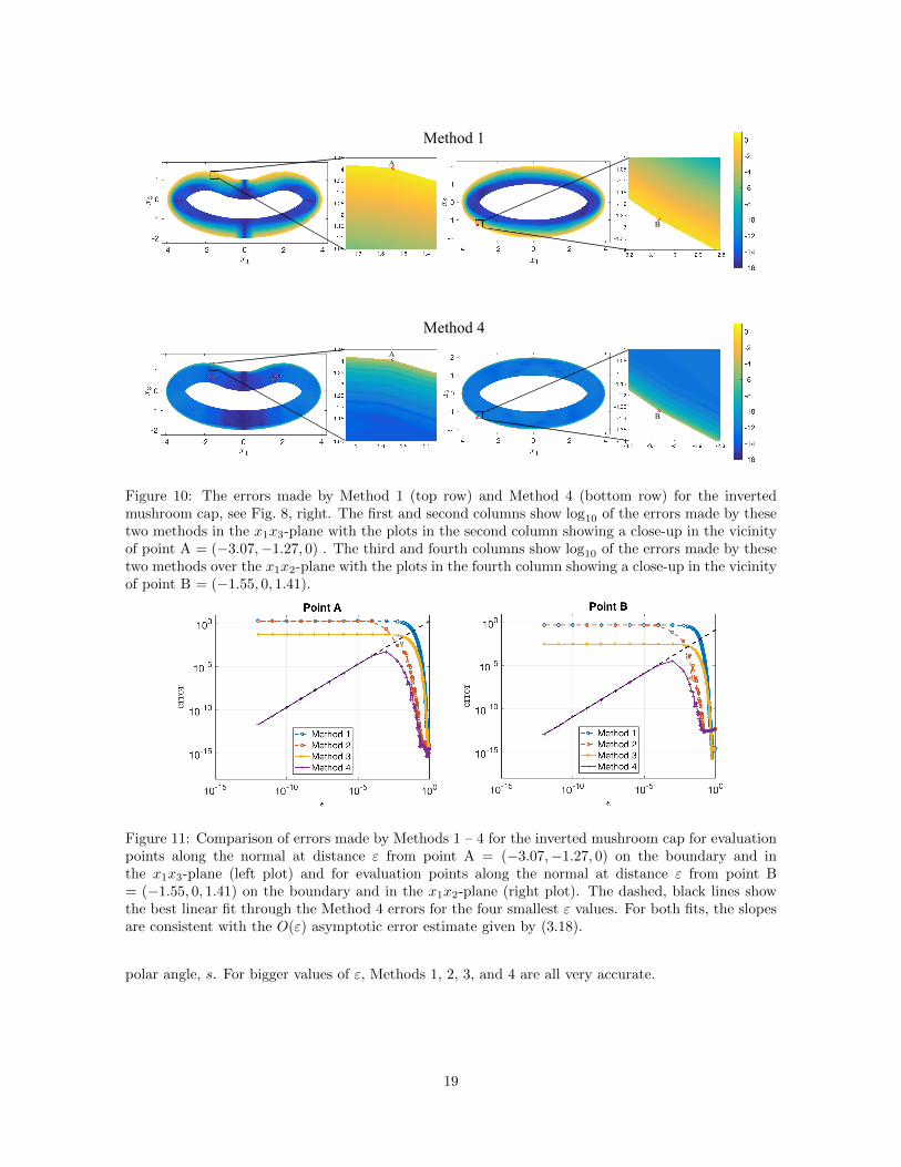
Figure 10: The errors made by Method 1 (top row) and Method 4 (bottom row) for the invertedmushroom cap, see Fig. 8, right. The first and second columns show log10 of the errors made by thesetwo methods in the x1x3-plane with the plots in the second column showing a close-up in the vicinityof point A = (−3.07,−1.27, 0) . The third and fourth columns show log10 of the errors made by thesetwo methods over the x1x2-plane with the plots in the fourth column showing a close-up in the vicinityof point B = (−1.55, 0, 1.41).

Figure 11: Comparison of errors made by Methods 1 – 4 for the inverted mushroom cap for evaluationpoints along the normal at distance ε from point A = (−3.07,−1.27, 0) on the boundary and inthe x1x3-plane (left plot) and for evaluation points along the normal at distance ε from point B= (−1.55, 0, 1.41) on the boundary and in the x1x2-plane (right plot). The dashed, black lines showthe best linear fit through the Method 4 errors for the four smallest ε values. For both fits, the slopesare consistent with the O(ε) asymptotic error estimate given by (3.18).

polar angle, s. For bigger values of ε, Methods 1, 2, 3, and 4 are all very accurate.

19

7 Conclusions

We have presented a simple and effective numerical method for the close evaluation of double- andsingle-layer potentials in three dimensions. The close evaluation of these layer potentials are challengingto numerically compute because they are nearly singular integrals. Based on a local analysis of theselayer potentials about the point at which their kernel is sharply peaked, we have identified a naturalway to compute those nearly singular integrals. This method consists of three steps:

1. Rotate the coordinate system so that the point at which the integrand is sharply peaked is alignedwith the north pole.

2. Integrate first with respect to the azimuthal angle using the Periodic Trapezoid Rule.

3. Integrate the remaining function with respect to the polar angle using the Gauss-LegendreQuadrature Rule mapped from [−1, 1] to [0, π].

A key point to Step 3 is that we do not integrate with respect to the cosine of the polar angle becausethe factor of sine of the polar angle (the natural Jacobian for the spherical coordinate system) isimportant in effectively computing these integrals. Numerical results presented here show that thelast step is essential for accurately computing these integrals. Moreover, the numerical results confirmthe asymptotic analysis results: the error for the modified double-layer potential due to the subtractionmethod decreases quadratically with respect to the distance from the boundary and the error for thesingle-layer potential decreases linearly with respect to the distance from the boundary.

This method is effective because integration with respect to azimuth in the rotated coordinate sys-tem is a natural averaging operation leading to a smooth function in the polar angle. This averagingoperation is a feature of the three-dimensional problem. It is not available for two-dimensional prob-lems. The results from the local analysis given by (3.11) and (3.18) show that this azimuthal averagingyields a function in the polar angle that has a finite limit at the north pole of the rotated coordinatesystem. Rather than use these results in a quadrature rule for the polar angle, we have chosen touse the Gauss-Legendre Quadrature Rule, which is an open rule, so that the quadrature points neverinclude the north and south poles. Therefore, these limiting values are not explicitly needed.

The local analysis used here can be extended to compute the full asymptotic expansions for theclose evaluation of double- and single-layer potentials. These asymptotic expansions can be used tofind approximations to a desired order of accuracy. Details of these asymptotic expansions can befound in [13]. These asymptotic expansions may be useful if one requires more accuracy for the closeevaluation of layer potentials. Nonetheless, we find that O(ε2) asymptotic error estimate for themodified double-layer potential and the O(ε) asymptotic error estimate for the single-layer potentialto be quite accurate. An asymptotic expansion for the single-layer potential may be useful to obtainan asymptotic error that matches that of the modified double-layer potential, for example.

We have assumed that the boundary is closed, oriented, and analytic in this paper, but as long asthe surface near the point on the boundary at which the integrand is singular is relatively smooth sothat there exists a natural averaging operation, one can apply this approach. Doing so may requireconsideration of different quadrature rules for that specific context.

Finally, the analysis shown here can be extended to other problems. In particular, this methodis broadly applicable to weakly singular and nearly singular integrals over two-dimensional surfaces.These weakly singular and nearly singular integrals may correspond to solutions of other elliptic partialdifferential equations including Helmholtz’s equation and Stokes’ equations.

A Rotations on the sphere

We give the explicit rotation formulas over the sphere used throughout this paper. Consider y, y? ∈ S2,the unit sphere. We introduce the parameters θ ∈ [0, π] and ϕ ∈ [−π, π] and write

y = y(θ, ϕ) = sin θ cosϕ ı + sin θ sinϕ + cos θ k. (A.1)

20

The specific parameters θ? and ϕ? are set so that y? = y(θ?, ϕ?). We would like to work in the rotated,uvw-coordinate system in which

u = cos θ? cosϕ? ı + cos θ? sinϕ? − sin θ? k,

v = − sinϕ? ı + cosϕ? ,

w = sin θ? cosϕ? ı + sin θ? sinϕ? + cos θ? k.

(A.2)

In this rotated system we have w = y?. For this rotated coordinate system, we introduce the parameterss ∈ [0, π] and t ∈ [−π, π] such that

y = y(s, t) = sin s cos t u + sin s sin t v + cos s w. (A.3)

It follows that w = y? = y(0, ·). This corresponds to setting y? to be the north pole. By equating(A.1) and (A.3) and substituting (A.2) into that result, we obtainsin θ cosϕ

sin θ sinϕcos θ

=

cos θ? cosϕ? − sinϕ? sin θ? cosϕ?

cos θ? sinϕ? cosϕ? sin θ? sinϕ?

− sin θ? 0 cos θ?

sin s cos tsin s sin t

cos s

. (A.4)

Let us rewrite (A.4) compactly as y(θ, ϕ) = R(θ?, ϕ?)y(s, t) with R(θ?, ϕ?) denoting the 3× 3 matrixgiven above. It is a rotation matrix. Hence, it is orthogonal.

We now seek to write θ = θ(s, t) and ϕ = ϕ(s, t). To do so, we introduce

ξ(s, t; θ?, ϕ?) = cos θ? cosϕ? sin s cos t− sinϕ? sin s sin t+ sin θ? cosϕ? cos s, (A.5)

η(s, t; θ?, ϕ?) = cos θ? sinϕ? sin s cos t+ cosϕ? sin s sin t+ sin θ? sinϕ? cos s, (A.6)

ζ(s, t; θ?, ϕ?) = − sin θ? sin s cos t+ cos θ? cos s. (A.7)

From (A.5) - (A.7), we find that

θ = arctan

(√ξ2 + η2

ζ

), (A.8)

and

ϕ = arctan

(η

ξ

). (A.9)

B Spherical Laplacian

In this Appendix, we establish the result given in (3.10). We first seek an expression for ∂2s [·]|s=0 interms of θ and ϕ. By the chain rule, we find that

∂2

∂s2[·]∣∣∣∣s=0

=

[(∂θ

∂s

)2∂2

∂θ2+

(∂ϕ

∂s

)2∂2

∂ϕ2+ 2

∂θ

∂s

∂ϕ

∂s

∂2

∂θ∂ϕ+∂2θ

∂s2∂

∂θ+∂2ϕ

∂s2∂

∂ϕ

] ∣∣∣∣s=0

. (B.1)

Using θ defined in (A.8) and ϕ defined in (A.9), we find that

∂θ(s, t)

∂s

∣∣∣∣s=0

= cos t, (B.2)

∂2θ(s, t)

∂s2

∣∣∣∣s=0

=cos θ?

sin θ?sin2 t, (B.3)

∂ϕ(s, t)

∂s

∣∣∣∣s=0

=sin t

sin θ?, (B.4)

∂2ϕ(s, t)

∂s2

∣∣∣∣s=0

= − cos θ?

sin2 θ?sin 2t. (B.5)

21

Note that at s = 0, we have θ? = θ.Substituting (B.2) – (B.5) into (B.1) and replacing θ? by θ, we obtain

∂2

∂s2[·]∣∣∣∣s=0

= cos2 t∂2

∂θ2+ sin2 t

1

sin2 θ

∂2

∂ϕ2+ 2 cos t sin t

1

sin θ

∂2

∂θ∂ϕ+ sin2 t

cos θ

sin θ

∂

∂θ− sin 2t

cos θ

sin2 θ

∂

∂ϕ,

(B.6)from which it follows that

1

π

∫ π

0

∂2

∂s2[·]∣∣∣∣s=0

dt =1

2

[∂2

∂θ2+

cos θ

sin θ

∂

∂θ+

1

sin2 θ

∂2

∂ϕ2

]=

1

2∆S2 , (B.7)

which establishes the result.

Acknowledgments

This research was supported by National Science Foundation Grant: DMS-1819052. A. D. Kim is alsosupported by the Air Force Office of Scientific Research Grant: FA9550-17-1-0238.

References

[1] L. af Klinteberg, A.-K. Tornberg, A fast integral equation method for solid particles in viscousflow using quadrature by expansion, J. Comput. Phys. 326 (2016) 420–445.

[2] L. af Klinteberg, A.-K. Tornberg, Error estimation for quadrature by expansion in layer potentialevaluation, Adv. Comput. Math. 43 (1) (2017) 195–234.

[3] K. E. Atkinson, Numerical integration on the sphere, ANZIAM J. 23 (3) (1982) 332–347.

[4] K. E. Atkinson, The numerical solution Laplace’s equation in three dimensions, SIAM J. Numer.Anal. 19 (2) (1982) 263–274.

[5] K. E. Atkinson, Algorithm 629: An integral equation program for Laplace’s equation in threedimensions, ACM Trans. Math. Softw. 11 (2) (1985) 85–96.

[6] K. E. Atkinson, A survey of boundary integral equation methods for the numerical solution ofLaplace’s equation in three dimensions, in: Numerical Solution of Integral Equations, Springer,1990, pp. 1–34.

[7] K. E. Atkinson, The Numerical Solution of Integral Equations of the Second Kind, CambridgeUniversity Press, 1997.

[8] A. H. Barnett, Evaluation of layer potentials close to the boundary for Laplace and Helmholtzproblems on analytic planar domains, SIAM J. Sci. Comput. 36 (2) (2014) A427–A451.

[9] J. T. Beale, M.-C. Lai, A method for computing nearly singular integrals, SIAM J. Numer. Anal.38 (6) (2001) 1902–1925.

[10] J. T. Beale, W. Ying, J. R. Wilson, A simple method for computing singular or nearly singularintegrals on closed surfaces, Commun. Comput. Phys. 20 (3) (2016) 733–753.

[11] O. P. Bruno, L. A. Kunyansky, A fast, high-order algorithm for the solution of surface scatteringproblems: basic implementation, tests, and applications, J. Comput. Phys. 169 (1) (2001) 80–110.

[12] C. Carvalho, S. Khatri, A. D. Kim, Asymptotic analysis for close evaluation of layer potentials,J. Comput. Phys. 355 (2018) 327–341.

22

[13] C. Carvalho, S. Khatri, A. D. Kim, Asymptotic approxiamtion for the close evaluation of double-layer potentials, In preparation.

[14] L. M. Delves, J. L. Mohamed, Computational Methods for Integral Equations, Cambridge Uni-versity Press, 1988.

[15] C. L. Epstein, L. Greengard, A. Klockner, On the convergence of local expansions of layer poten-tials, SIAM J. Numer. Anal. 51 (5) (2013) 2660–2679.

[16] R. B. Guenther, J. W. Lee, Partial Differential Equations of Mathematical Physics and IntegralEquations, Dover Publications, 1996.

[17] J. Helsing, R. Ojala, On the evaluation of layer potentials close to their sources, J. Comput. Phys.227 (5) (2008) 2899–2921.

[18] A. Klockner, A. Barnett, L. Greengard, M. O’Neil, Quadrature by expansion: A new method forthe evaluation of layer potentials, J. Comput. Phys. 252 (2013) 332–349.

[19] M. Rachh, A. Klockner, M. O’Neil, Fast algorithms for quadrature by expansion i: Globally validexpansions, J. Comput. Phys. 345 (2017) 706–731.

[20] C. Schwab, W. Wendland, On the extraction technique in boundary integral equations, Math.Comput. 68 (225) (1999) 91–122.

[21] M. Wala, A. Klockner, A fast algorithm for Quadrature by Expansion in three dimensions,arXiv:1805.06106v1.

23