Atmos. Chem. Phys., 12, 3349–3362, 2012www.atmos-chem-phys.net/12/3349/2012/doi:10.5194/acp-12-3349-2012© Author(s) 2012. CC Attribution 3.0 License.

AtmosphericChemistry

and Physics

Climatic effects of 1950–2050 changes in US anthropogenicaerosols – Part 2: Climate response

E. M. Leibensperger1,*, L. J. Mickley 1, D. J. Jacob1, W.-T. Chen2, J. H. Seinfeld3, A. Nenes4, P. J. Adams5,D. G. Streets6, N. Kumar7, and D. Rind8

1School of Engineering and Applied Sciences, Harvard University, Cambridge, MA, USA2Jet Propulsion Laboratory, California Institute of Technology, Pasadena, CA, USA3Division of Chemistry and Chemical Engineering, California Institute of Technology, Pasadena, CA, USA4School of Earth & Atmospheric Sciences and School of Chemical & Biological Engineering, Georgia Institute ofTechnology, Atlanta, GA, USA5Department of Civil & Environmental Engineering and Department of Engineering & Public Policy, Carnegie MellonUniversity, Pittsburgh, PA, USA6Argonne National Laboratory, Argonne, IL, USA7Electric Power Research Institute, Palo Alto, CA, USA8NASA Goddard Institute for Space Studies, New York, NY, USA* now at: Dept. of Earth, Atmospheric and Planetary Sciences, Massachusetts Institute of Technology, Cambridge, MA, USA

Correspondence to:E. M. Leibensperger (eleibens@mit.edu)

Received: 20 May 2011 – Published in Atmos. Chem. Phys. Discuss.: 29 August 2011Revised: 14 December 2011 – Accepted: 22 February 2012 – Published: 10 April 2012

Abstract. We investigate the climate response to chang-ing US anthropogenic aerosol sources over the 1950–2050period by using the NASA GISS general circulation model(GCM) and comparing to observed US temperature trends.Time-dependent aerosol distributions are generated from theGEOS-Chem chemical transport model applied to historicalemission inventories and future projections. Radiative forc-ing from US anthropogenic aerosols peaked in 1970–1990and has strongly declined since due to air quality regula-tions. We find that the regional radiative forcing from USanthropogenic aerosols elicits a strong regional climate re-sponse, cooling the central and eastern US by 0.5–1.0◦Con average during 1970–1990, with the strongest effectson maximum daytime temperatures in summer and autumn.Aerosol cooling reflects comparable contributions from di-rect and indirect (cloud-mediated) radiative effects. Absorb-ing aerosol (mainly black carbon) has negligible warming ef-fect. Aerosol cooling reduces surface evaporation and thusdecreases precipitation along the US east coast, but also in-creases the southerly flow of moisture from the Gulf of Mex-ico resulting in increased cloud cover and precipitation in thecentral US. Observations over the eastern US show a lackof warming in 1960–1980 followed by very rapid warmingsince, which we reproduce in the GCM and attribute to trends

in US anthropogenic aerosol sources. Present US aerosolconcentrations are sufficiently low that future air quality im-provements are projected to cause little further warming inthe US (0.1◦C over 2010–2050). We find that most of thewarming from aerosol source controls in the US has alreadybeen realized over the 1980–2010 period.

1 Introduction

Global mean surface temperatures increased by0.74± 0.18◦C between 1906 and 2005 due to increas-ing greenhouse gases (Trenberth et al., 2007). However,temperature trends on regional scales are more compli-cated. For example, the eastern US experienced a coolingbetween 1930 and 1990 (Fig. 1). The net cooling effect ofanthropogenic aerosols is known to have mitigated some ofthe global warming from greenhouse gases (Hegerl et al.,2007), but the importance of aerosol cooling on temperaturetrends in the US has received little attention. As US aerosolsources are increasingly controlled to improve air quality,the associated cooling is undone resulting in acceleratedwarming (Andreae et al., 2005; Brasseur and Roeckner,2005; Kloster et al., 2009; Mickley et al., 2012). Air quality

Published by Copernicus Publications on behalf of the European Geosciences Union.

3350 E. M. Leibensperger et al.: Climate response

-1.00 -0.50 -0.20 -0.05 0.10 0.30 0.75

Observed 1930-1990 Change in Annual Mean Surface Air Temperature (ºC)

-0.75 -0.30 -0.10 0.05 0.20 0.50 1.00

Fig. 1. Observed change in surface air temperature between 1930and 1990. Temperature change is based on the linear trend as inHansen et al. (2001). Observations are from the NASA GISS Sur-face Temperature Analysis (GISTEMP;http://data.giss.nasa.gov/gistemp/).

improvement thus comes with climate consequences (Raesand Seinfeld, 2009). In Leibensperger et al. (2012), wereconstructed and projected the aerosol trends and associatedradiative forcing from US anthropogenic sources over the1950–2050 period. US aerosol concentrations peaked in1970–1990 and have decreased rapidly since. We use herea general circulation model (GCM) to study the associatedclimate response.

Anthropogenic aerosols directly affect the climate systemby scattering and absorbing solar radiation, and indirectly byaltering cloud microphysical properties. Aerosol scatteringcools and absorption warms the atmosphere, but both causea reduction in surface solar radiation. Observations of sur-face solar radiation over the US show a widespread decreaseover the 1950–1990 period followed by a more recent in-crease (Liepert and Tegen, 2002; Long et al., 2009). Thesetrends have been identified in clear and all-sky scenes, sug-gesting a role for both direct and indirect aerosol effects.These trends in surface solar radiation are qualitatively con-sistent with changes in aerosol sources (Streets et al., 2009),but cannot be entirely explained by anthropogenic aerosols(Liepert and Tegen, 2002; Long et al., 2009; Wild, 2009b;Koch et al., 2011).

Aerosols are scavenged from the atmosphere by precipita-tion on a time scale of days, so that their radiative forcing isstrongly localized over source regions (Schulz et al., 2006).A critical issue is whether the regional radiative forcing ofaerosols elicits a correspondingly regional climate response.Observation-based studies have related changes in surfacesolar radiation with other climate variables as a method ofdeducing the local effects of aerosol forcing. They show evi-dence that aerosols have lowered surface air temperature andtemporarily offset greenhouse warming (Qian and Giorgi,

2000; Wild et al., 2007; Ruckstuhl et al., 2008; Philipona etal., 2009), reduced the diurnal temperature range by damp-ening daily maximum temperatures (Liu et al., 2004b; Wildet al., 2007; Makowski et al., 2009), lowered evaporationrates (Peterson et al., 1995; Liu et al., 2004a; Roderick et al.,2007), and increased soil moisture (Robock et al., 2005).

Some GCM studies have found strong regional climatesensitivity to aerosols including in India (Menon et al., 2002;Wang et al., 2009a), southeast Asia (Chang et al., 2009;Zhang et al., 2011; Lee and Kim, 2010), the North At-lantic (Fischer-Bruns et al., 2009), and the western US (Ja-cobson, 2008). However, other studies have found that theclimate response to aerosol radiative forcing is more hemi-spheric or global in scale with patterns similar (but oppo-site in sign) to greenhouse gas forcing (Mitchell et al., 1995;Shindell et al., 2007, 2008; Levy et al., 2008; Kloster et al.,2009). Shindell et al. (2010) estimated the spatial extentof the climate response to aerosol radiative forcing in fourGCMs and found it to extend∼3500 km in the meridionaldirection and∼12 000 km in the zonal direction. Fischer-Bruns et al. (2010) investigated the climate impacts of re-moving North American aerosols and found a 1.0–1.5◦Csummer warming in surface air over the US and North At-lantic Ocean. They also found a 1.5–2.0◦C warming of theArctic in winter. However, Mickley et al. (2012) simulatedthe climate response of completely removing aerosols overthe US and found a 0.4–0.6◦C regional warming in the USwith little effect elsewhere.

There is strong motivation for air quality agencies to de-crease aerosol concentrations to improve public health. Bet-ter understanding of the associated climate response is nec-essary. The US is of particular interest in this regard be-cause aerosol concentrations rose in the 20th century, peakedin the 1980s, and have been decreasing rapidly since duein large part to a 56 % reduction of SO2 emissions between1980 and 2008 (US EPA, 2010). Here we use the 1950–2050time series of US aerosol concentrations from Leibenspergeret al. (2012) to conduct 1950–2050 transient climate simu-lations with the NASA Goddard Institute for Space Studies(GISS) GCM 3 (Rind et al., 2007). Our objective is to inves-tigate the regional climate effects of historical and projectedchanges in US anthropogenic aerosol sources. An importantadvance compared to previous work is the use of a realisticevolution of aerosol sources.

2 Methods

We conduct sensitivity simulations with the GISS GCM 3to study the evolving 1950–2050 climate response to chang-ing US anthropogenic aerosol sources. The GCM usesarchived global 3-D monthly mean concentrations of dif-ferent aerosol components from the GEOS-Chem chemi-cal transport model (CTM) with time-dependent emissionsbased on historical data and future projections. The CTM

Atmos. Chem. Phys., 12, 3349–3362, 2012 www.atmos-chem-phys.net/12/3349/2012/

E. M. Leibensperger et al.: Climate response 3351

simulations are described by Leibensperger et al. (2012) anda brief summary is given below.

2.1 Aerosol simulations

We conduct a 2-yr GEOS-Chem simulation of coupledozone-NOx-VOC-aerosol chemistry (http://geos-chem.org;Bey et al., 2001; Park et al., 2004) for each decade between1950 and 2050. The first year is used as model initializa-tion. Monthly mean fine aerosol concentrations are archivedfrom the second year for use in the GCM including sulfate-nitrate-ammonium (SNA), primary organic aerosol (POA),secondary organic aerosol (SOA), and black carbon (BC)(Park et al., 2006; Liao et al., 2007). Simulations for all yearsuse the same assimilated meteorological data from 2000–2001 so that changes in concentrations over the 1950–2050period are due to emissions only. The meteorological data arefrom the NASA Goddard Earth Observing System (GEOS)-4with 1◦

× 1.25◦ horizontal resolution, 55 vertical levels, and6-h temporal resolution (3-h for surface variables and mixingdepths). The horizontal resolution is degraded to 2◦

× 2.5◦

for input to GEOS-Chem. The effect of US anthropogenicsources is determined by parallel sensitivity simulations forthe 1950–2050 period with zero US anthropogenic emissionsof SO2, NOx, POA, and BC. “Anthropogenic” here includesfuel and industrial sources but not open fires.

We use 1950–1990 global anthropogenic emissions of SO2and NOx from EDGAR Hyde 1.3 (van Aardenne et al.,2001) and 2000 emissions from EDGAR 3.2 FT (Olivierand Berdowski, 2001). Historical emissions of BC and POAare from Bond et al. (2007). Emissions past 2000 are cal-culated using growth factors derived from the IntegratedModel to Assess the Greenhouse Effect (IMAGE; Streets etal., 2004) following the IPCC A1B scenario (Nakicenovicand Swart, 2000). As in Fiore et al. (2002) and Wu etal. (2008), growth factors are calculated for different coun-tries and fuel types (fossil fuel and biofuel). Ammonia emis-sions are from Bouwman et al. (1997) as modified by Park etal. (2004), except for East Asia (Streets et al., 2003). Addi-tional sources include climatological biomass burning (Dun-can et al., 2003), fertilizer (Wang et al., 1998), aircraft (Chinet al., 2000), the biosphere, volcanoes, and lightning. SeeLeibensperger et al. (2012) for more detail.

2.2 Climate simulations

We conduct transient climate simulations with the GISSGCM 3 using a horizontal resolution of 4◦

× 5◦ and 23 ver-tical levels that extend from the surface to 0.002 hPa. GISSGCM 3 shares a common history with another NASA GISSGCM, Model E (Schmidt et al., 2006), but the two differ intheir parameterizations of gravity wave drag, convection, andthe boundary layer (Rind et al., 2007). GISS GCM 3 has beenpreviously used in studies investigating air quality-climateinteractions (Leibensperger et al., 2008; Wu et al., 2008; Pye

et al., 2009; Chen et al., 2010b; Mickley et al., 2012), tracertransport (Rind et al., 2007), climate response to solar forc-ing (Rind et al., 2008), and stratospheric ozone-climate in-teractions (Rind et al., 2009a, b). The model contains a Q-flux ocean, in which monthly oceanic heat transports are heldconstant but sea surface temperature and sea ice coverage areallowed to respond to energy exchange with the atmosphere(Hansen et al., 1988). We calculate ocean heat transport us-ing equilibrium climate simulations forced with observed seasurface temperature (SST) and sea ice distributions for 1946–1955 (Rayner et al., 2003), following the method outlined byHansen et al. (1988).

To compute the aerosol direct effect, we import 3-Dmonthly mean aerosol concentrations archived from GEOS-Chem. Concentrations are interpolated between decadal timeslices. Aerosol optical properties are calculated assuming aninternal mixture. Following Chung and Seinfeld (2002) andLiao et al. (2004), we assume a standard gamma aerosol sizedistribution with an effective dry radius of 0.3 µm and area-weighted variance of 0.2. Optical properties of the internalmixture are calculated using the volume-weighted mean ofthe refractive indices of the individual components. The re-sulting direct forcing from US anthropogenic aerosol sourcesin 1980 (peak aerosol loading) is only−0.07 W m−2 globallybut −2.0 W m−2 over the eastern US (Leibensperger et al.,2012). Dust and sea salt aerosols are considered externallymixed and held constant for 1950–2050 at the climatologicalradiative forcing values of Hansen et al. (2002).

Aerosol indirect radiative effects are computed followingthe approach previously implemented by Chen et al. (2010b)in the GISS GCM 3. This includes the first indirect effect(cloud albedo) and the second indirect effect (cloud lifetime),both on liquid stratiform clouds only. Aerosol mass con-centrations affect the cloud droplet number concentrationNc(m−3), which in turn determines the effective radius of clouddroplets and the rate of autoconversion to precipitation. WecalculateNc from the archived GEOS-Chem aerosol massdistributions using the method of Chen et al. (2010b):

logNc = A+B logmi (1)

wheremi is the molar concentration of dissolved aerosol ions(mol m−3) andA andB are gridded 3-D monthly mean co-efficients derived from detailed simulations of aerosol mi-crophysics and activation within the GCM (Adams and Sein-feld, 2002; Nenes and Seinfeld, 2003; Fountoukis and Nenes,2005; Pierce and Adams, 2006). Cloud optical depth scalesas the inverse of the area-weighted mean effective radiusreof the cloud droplet size distribution (Del Genio et al., 1996).We obtainre from:

re= κ−13

[3L

4πNc

] 13

(2)

whereL is the liquid water content of the cloud (cm3 waterper cm−3 air), andκ is a constant (0.67 over land, 0.80 over

www.atmos-chem-phys.net/12/3349/2012/ Atmos. Chem. Phys., 12, 3349–3362, 2012

3352 E. M. Leibensperger et al.: Climate response

ocean; Martin et al., 1994) that relates the volume-weightedand area-weighted mean radii. Autoconversion rates are cal-culated using the parameterization of Khairoutdinov and Ko-gan (2000), which fits results from an explicit microphysicalmodel:

dql

dt= −1350γ q2.47

l N−1.79c (3)

whereql is the cloudwater mass content (kg kg−1). Hoose etal. (2008) and Chen et al. (2010b) added the tuning parameterγ in order to retain GCM climate equilibrium. We find thata γ value of 12 retains top-of-atmosphere (TOA) radiativebalance in a climate equilibrium simulation for 1950 condi-tions including fixed SST and sea ice (Leibensperger et al.,2012).γ = 12 is consistent with the recent results of Moralesand Nenes (2010), who found that autoconversion rates canbe underestimated by a factor of 2 to 10 when models usegridbox-scale values ofNc.

Two sets of control simulations were conducted. The firstincludes only the direct radiative forcing from aerosols, usingthe imported aerosol concentrations from GEOS-Chem. Thesecond additionally importsNc as calculated in Eq. (1) to ac-count for the aerosol indirect effects. Sensitivity simulationswere conducted relative to each of these controls using theaerosol andNc fields from the GEOS-Chem simulations withUS anthropogenic sources of SO2, NOx, POA, and BC shutoff. Differences between the control and sensitivity simula-tions then measure the climate response to US anthropogenicsources through the direct and indirect effects of aerosols.

Each set of simulations consists of a five-member ensem-ble conducted from 1950 to 2050 using the trends in nat-ural and greenhouse gas forcing described by Hansen etal. (2002). Future greenhouse gas concentrations follow theIPCC SRES A1B scenario with CO2, N2O, and CH4 reach-ing 522, 0.350, and 2.40 ppm, respectively, by 2050. TheA1B scenario provides a radiative forcing for the 21st cen-tury comparable to the more recent RCP6 scenario from theIPCC (Moss et al., 2010). Initiating climate simulations from1950 equilibrium conditions neglects the small radiative im-balance that occurred at that time. A previous study with theGISS GCM using the same climate forcing as here (exceptfor tropospheric aerosols) found the Earth to be out of radia-tive balance by +0.18 W m−2 for 1951 conditions (Sun andHansen, 2003). This suggests that our simulations underes-timate post-1950 global warming by approximately 0.1◦C, asmall effect that does not impact our assessment of the cli-mate response to US anthropogenic aerosols since it is com-mon to both the control and sensitivity simulations.

We conducted an additional sensitivity simulation to iso-late the climate effects of US anthropogenic sources of BC.This simulation uses the sulfate, nitrate, POA, and SOA dis-tributions from the control simulation, but no BC emissionfrom US anthropogenic sources. Results indicate that theclimate effects of US anthropogenic BC are small and indis-tinguishable from interannual variability. This is consistent

with the weak radiative forcing from US anthropogenic BC(+0.02 W m−2 globally and +0.4 W m−2 over the eastern USfor 1970–1990; Leibensperger et al., 2012). More generally,we find that a regional radiative forcing of about 1.0 W m−2

is necessary to produce a climate response greater than natu-ral variability in the GISS GCM 3 with a 5-member ensem-ble. The climate effects of BC may differ when consider-ing co-emitted species and microphysical effects (Bauer etal., 2010; Chen et al., 2010a; Jacobson, 2010). The climateeffects of BC are additionally sensitive to the vertical pro-file of BC and modeled cloud cover (Koch and Del Genio,2010). Koch et al. (2011) found surface air temperature to beless sensitive to BC than a similar amount of sulfate radiativeforcing due to compensating changes in stability and cloudcover. Previous studies have shown a significant climate re-sponse in Asia where BC radiative forcing is greater (Menonet al., 2002; Wang et al., 2009a), but this region has largerBC emissions. We do not discuss this simulation further.

The use of archived monthly mean aerosol distributionsas input to our climate simulations does not allow for feed-backs of changing climate on aerosol concentrations. Thesefeedbacks are likely very small relative to the source drivenaerosol perturbations implemented here, considering thatboth models and observations indicate little direct sensitivityof aerosol air quality to climate change (Jacob and Winner,2009; Tai et al., 2011). The use of monthly mean aerosolconcentrations does not introduce significant bias in the cal-culation of the direct radiative effect (Koch et al., 1999), butit may affect the aerosol indirect effect due to the nonlinearrelationship between aerosol amount and cloud droplet num-ber (Jones et al., 2001) as seen in Eq. (1).

We test the statistical significance of all our results usinga modified version of Student’s t-test to account for serialcorrelation (Zwiers and von Storch, 1995). Results presentedhere are significant at the 95th percentile and represent themean of ensemble members unless specified.

3 Climate response to US anthropogenic aerosols

3.1 Radiation

Figure 2 shows the annual mean change in net TOA and sur-face solar radiation due to the direct and indirect radiativeeffects of US anthropogenic aerosols in 1970–1990, the pe-riod when US aerosol loadings were at their peak. These dif-fer from the radiative forcings reported by Leibensperger etal. (2012) in that they include the effects of climate response,such as changes in cloud cover. We find that the radiative ef-fect is strongly concentrated over the eastern US, and definea mid-Atlantic US region boxed in Fig. 2 where the effect ismaximum. The annual mean TOA radiative effect averages−6 W m−2 over that region, whereas the global TOA radia-tive effect is only−0.08 W m−2.

Atmos. Chem. Phys., 12, 3349–3362, 2012 www.atmos-chem-phys.net/12/3349/2012/

E. M. Leibensperger et al.: Climate response 3353

Aerosol Direct EffectAerosol Direct + Indirect Effects

1950 1970 1990 2010 2030 2050Year

-8

-4

-2

0

2

∆ R

adia

tion

(W m

-2)

1950 1970 1990 2010 2030 2050Year

-10

-8

-6

-4

0

2

∆ Top of Atmosphere Radiation (W m-2) ∆ Surface Solar Radiation (W m-2)

-12 -10 -8 -6 -4 42 108-2 6 12-1 1

-2

-6Net Top of Atmosphere Surface Solar

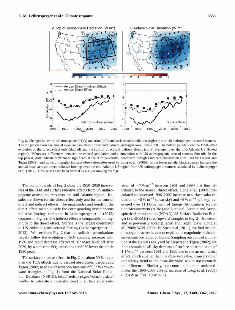
Fig. 2. Changes in net top-of-atmosphere (TOA) radiation (left) and surface solar radiation (right) due to US anthropogenic aerosol sources.The top panels show the annual mean aerosol effect (direct and indirect) averaged over 1970–1990. The bottom panels show the 1950–2050evolution of the direct effect only (dashed) and the sum of direct and indirect effects (solid) averaged over the mid-Atlantic US (boxedregion). Values are differences between the control simulation and a simulation with US anthropogenic aerosol sources shut off. In thetop panels, dots indicate differences significant at the 95th percentile, downward triangles indicate observation sites used by Liepert andTegen (2002), and upward triangles indicate observation sites used by Long et al. (2009). In the lower panels, black squares indicate theannual mean aerosol direct radiative forcings over the mid-Atlantic US region from US anthropogenic sources calculated by Leibenspergeret al. (2012). Time series have been filtered by a 15-yr moving average.

The bottom panels of Fig. 2 show the 1950–2050 time se-ries of the TOA and surface radiative effects from US anthro-pogenic aerosol sources over the mid-Atlantic region. Re-sults are shown for the direct effect only and for the sum ofdirect and indirect effects. The magnitudes and trends of thedirect effect match closely the corresponding instantaneousradiative forcings computed in Leibensperger et al. (2012)(squares in Fig. 2). The indirect effect is comparable in mag-nitude to the direct effect. Sulfate is the largest contributorto US anthropogenic aerosol forcing (Leibensperger et al.,2012). We see from Fig. 2 that the radiative perturbationslargely follow the evolution of SO2 sources: increase until1980 and rapid decrease afterward. Changes level off after2020, by which time SO2 emissions are 80 % lower than their1980 peak.

The surface radiative effects in Fig. 2 are about 50 % largerthan the TOA effects due to aerosol absorption. Liepert andTegen (2002) used six observation sites east of 95◦ W (down-ward triangles in Fig. 1) from the National Solar Radia-tion Database (NSRDB;http://rredc.nrel.gov/solar/olddata/nsrdb/) to estimate a clear-sky trend in surface solar radi-

ation of −7 W m−2 between 1961 and 1990 that they at-tributed to the aerosol direct effect. Long et al. (2009) cal-culated an observed 1996–2007 increase in surface solar ra-diation of +5 W m−2 (clear sky) and +8 W m−2 (all sky) av-eraged over 11 Department of Energy Atmospheric Radia-tion Measurement (ARM) and National Oceanic and Atmo-spheric Administration (NOAA) US Surface Radiation Bud-get (SURFRAD) sites (upward triangles in Fig. 2). However,and as previously noted (Liepert and Tegen, 2002; Long etal., 2009; Wild, 2009a, b; Koch et al., 2011), we find that an-thropogenic aerosols cannot explain the magnitude of the ob-served surface radiation trends. Sampling our control simula-tion at the six sites analyzed by Liepert and Tegen (2002), wefind a simulated all-sky decrease of surface solar radiation of1.1 W m−2 between 1961 and 1990 due to the aerosol directeffect, much smaller than the observed value. Conversion ofour all-sky trend to the clear-sky value would not reconcilethe difference. Similarly, our control simulation underesti-mates the 1996–2007 all-sky increase of Long et al. (2009)(+2.4 W m−2 vs. +8 W m−2).

www.atmos-chem-phys.net/12/3349/2012/ Atmos. Chem. Phys., 12, 3349–3362, 2012

3354 E. M. Leibensperger et al.: Climate response

We previously showed that our simulated trend of sulfateover the US is in good agreement with observations, at leastfor 1990–present, while the simulated decreasing trend ofblack carbon is too low by a factor of 2 (Leibensperger etal., 2012). Correcting for this discrepancy does not recon-cile the simulated and observed 1996–2007 trends in solarradiation. The observed surface solar radiation trends remainlarger than our simulated trends and thus seem much largerthan can be explained from aerosol trends. The discrepancyseems unlikely to arise from underestimated aerosol radiativeeffects since models consistently underestimate the observedtrend (Liepert and Tegen, 2002; Long et al., 2009; Wild,2009a, b; Koch et al., 2011). The 1961–1990 NSRDB sur-face solar radiation data suffer from inconsistent data qual-ity, but the more recent measurements presented by Long etal. (2009) have consistent annual calibration and daily per-formance monitoring. The cause of the model-observationdiscrepancy is unclear but suggests that observed trends insurface radiation are not driven solely by aerosols.

3.2 Temperature

Figure 3 shows the annual mean temperature changes in sur-face air and at 500 hPa due to the direct and indirect effectsof US anthropogenic aerosol sources over the 1970–1990 pe-riod when US anthropogenic aerosol forcing was at its peak.Changes in surface air temperature are largest in the east-ern US (0.5–1.0◦C cooling), collocated with the maximumradiative effect (Fig. 2). The cooling influence of US anthro-pogenic aerosols extends over much of the Northern Hemi-sphere, but beyond the US and North Atlantic Ocean it isonly marginally significant against modeled interannual vari-ability. The annual mean cooling averages 0.1◦C for theNorthern Hemisphere and 0.05◦C for the Southern Hemi-sphere.

We find that the cooling effect of US anthropogenicaerosols is largely confined to the US and North Atlantic. Aspointed out in the Introduction, Shindell et al. (2010) esti-mated the spatial extent of the climate response to aerosol ra-diative forcing to span∼3500 km in the meridional directionand∼12 000 km in the zonal direction. We find in our sim-ulation that some cooling from US anthropogenic aerosolsextends to these distances but is only marginally significantor insignificant. The cooling within the US caused by USanthropogenic aerosols shown in Fig. 3 is not apparent inthe simulations of Shindell et al. (2010), which simulatedthe climate response of all anthropogenic aerosols. However,cooling within the US can be found in other simulations ofthe climate effects of anthropogenic aerosols (Mitchell et al.,1995; Hansen et al., 2005; Wilcox et al., 2009; Mickley etal., 2012).

Cooling is more diffuse at higher altitudes, reflecting thefaster transport of heat (Fig. 3, top). At 500 hPa, the largestcooling is 0.3◦C over the eastern US and North AtlanticOcean. Statistically significant cooling covers more of the

500 hPa

SURFACE AIR

Change in Annual Mean Temperature (°C)

-1.00

-0.75

-0.50

-0.40

-0.30

-0.20

-0.10

-0.05

0.05

0.10

0.20

0.30

0.40

0.50

0.75

1.00

Fig. 3. Effect of US anthropogenic aerosol sources on annual meantemperatures (◦C) for the 1970–1990 period (when US aerosol load-ing was at its peak). Values are shown for surface air (bottom) and500 hPa (top) temperatures. They represent the mean difference be-tween 5-member ensemble GCM simulations including vs. exclud-ing US anthropogenic aerosol sources, and considering both aerosoldirect and indirect effects. Dots indicate differences significant atthe 95th percentile.

Northern Hemisphere at 500 hPa than at the surface. An-nual mean cooling at 500 hPa averages 0.1◦C for the North-ern Hemisphere and 0.02◦C for the Southern Hemisphere,similar to the hemispheric changes in surface air tempera-ture. Cooling is even more diffuse at 300 hPa (not shown),but Northern Hemisphere cooling is similarly 0.1◦C.

Figure 4 shows the surface air cooling over the US dueto US anthropogenic aerosols for the 1970–1990 period forthe simulations including only the aerosol direct effect (top)and the combination of direct and indirect effects (bottom).The bottom panel is a zoomed version of the bottom panelof Fig. 3. Significant cooling extends over much of the USeven when the aerosol direct effect alone is considered. Themagnitude of the cooling doubles when the indirect effectsare included but the spatial patterns are similar. Thus the sig-nificance and localization of the US cooling due to US an-thropogenic aerosol sources is not contingent on the indirecteffects, which are far more uncertain than the direct effect.

Atmos. Chem. Phys., 12, 3349–3362, 2012 www.atmos-chem-phys.net/12/3349/2012/

E. M. Leibensperger et al.: Climate response 3355

Change in Annual Mean Surface Air Temperature (˚C)

Aerosol Direct and Indirect Effects

-1.00-0.75-0.50-0.40-0.30-0.20-0.10 0.10 0.20 0.30 0.40 0.50 0.75 1.00

Aerosol Direct Effect

Fig. 4. Effect of US anthropogenic aerosol sources on surface airtemperatures for the 1970–1990 period when US aerosol loadingwas at its peak. Values represent the mean difference between 5-member ensemble GCM simulations including vs. excluding USanthropogenic aerosol sources, and considering the aerosol directonly (top) and the sum of direct and indirect effects (bottom). Dotsindicate differences significant at the 95th percentile. The bottompanel contains the same information as the bottom panel of Fig. 3but zoomed over the US.

Cooling is strongest in the Midwest, shifted westward rela-tive to the surface and TOA radiative effects shown in Fig. 2.This is due to hydrological factors and is discussed further inSect. 3.3.

Figure 5 shows seasonal statistics of the effects of US an-thropogenic aerosols on surface air temperatures in the mid-Atlantic US (boxed region in Fig. 2). The change in surfaceair temperature is largest in summer and autumn, with re-gionally averaged cooling of more than 1.0◦C in autumn.Aerosol radiative forcing is largest in summer when solarradiation is strongest. The larger surface air temperaturechanges in autumn reflect the drier conditions typical of thattime of year, so that less of the radiative effect is buffered bychanges in surface evaporation (latent heat flux).

Figure 5 also presents the changes in extreme tempera-tures. We find that aerosol cooling has a larger effect on

MAM JJA SON DJF Season

-2.0

-1.5

-1.0

-0.5

0.0

0.5

Cha

nge

in S

urfa

ce A

ir T

empe

ratu

re (

˚C)

5th Percentile Daily Minimum TemperatureMean Daily Minimum TemperatureMean TemperatureMean Daily Maximum Temperature95th Percentile Daily Maximum Temperature

Fig. 5. Effect of US anthropogenic aerosols on seasonal surfaceair temperature statistics over the mid-Atlantic US (boxed region inFig. 2). Values are for 1970–1990, when US aerosol loads wereat their peak. Statistics were obtained by difference between 5-member ensemble GCM simulations including vs. excluding US an-thropogenic aerosol sources, and considering both the aerosol directand indirect effects. Error bars indicate 95 % confidence intervals.

daily maximum than daily minimum temperatures, in all sea-sons, as expected since the forcing is due to scattering ofsolar radiation. The cooling is largest during heat waves ofsummer and autumn (95th percentile daily maximum tem-peratures, corresponding to the 5 hottest days of each sea-son). These heat waves occur under cloud free conditionswhen the aerosol direct effect is especially effective. We findthat the warmest days are cooler by 1.0◦C in summer and1.3◦C in autumn. The coldest nights of each season (5thpercentile daily minimum temperatures) are least sensitive toaerosols except in winter when they are typically associatedwith synoptic-scale clear-sky conditions.

The model pattern of aerosol-driven cooling over the USin Fig. 4 is remarkably similar to the observed pattern inthe 1930–1990 trend in surface air temperature shown inFig. 1. The largest area of cooling in the central US haspreviously been referred to as a “warming hole” (Pan et al.,2004; Kunkel et al., 2006). Previous GCM studies have as-sociated this warming hole with variations in SSTs in thetropical Pacific (Robinson et al., 2002; Kunkel et al., 2006;Wang et al., 2009b). Kunkel et al. (2006) additionally pointout a strong association between the observed variability ofNorth Atlantic SSTs and central US surface temperatures.Our results indicate that the warming hole could be due toUS anthropogenic aerosols, as SO2 anthropogenic emissionsin 1930 were only 60 % of those in 1980. We find that US an-thropogenic aerosols lower SSTs in the North Atlantic regionoutlined by Kunkel et al. (2006) by up to−0.3◦C. LowerSSTs over the North Atlantic enhance the anticyclonic trans-port of marine air over the Gulf Coast of the US, magnifyingthe cooling as discussed below.

www.atmos-chem-phys.net/12/3349/2012/ Atmos. Chem. Phys., 12, 3349–3362, 2012

3356 E. M. Leibensperger et al.: Climate response

d) Soil Moisture Availability (%)

-5.00 -1.25 0.00 1.25 2.50 3.75 5.00

-2.50-3.75 -4 -3 -2 -1 0 1 2 3 4

c) Cloud Cover (%)

b) Precipitation (mm day-1)

-0.30 -0.20 -0.10 -0.05 -0.02 0.02 0.05 0.10 0.20 0.30

a) Evaporation (mm day-1)

-0.30 -0.20 -0.10 -0.05 -0.02 0.02 0.05 0.10 0.20 0.30

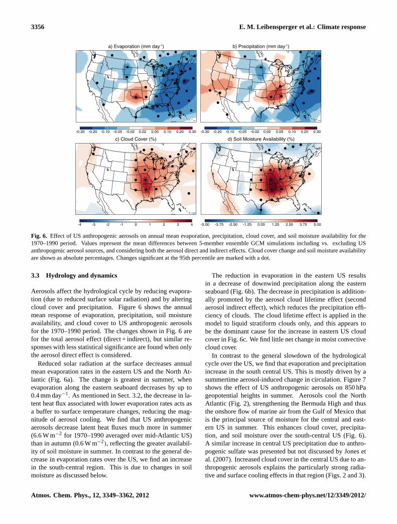
Fig. 6. Effect of US anthropogenic aerosols on annual mean evaporation, precipitation, cloud cover, and soil moisture availability for the1970–1990 period. Values represent the mean differences between 5-member ensemble GCM simulations including vs. excluding USanthropogenic aerosol sources, and considering both the aerosol direct and indirect effects. Cloud cover change and soil moisture availabilityare shown as absolute percentages. Changes significant at the 95th percentile are marked with a dot.

3.3 Hydrology and dynamics

Aerosols affect the hydrological cycle by reducing evapora-tion (due to reduced surface solar radiation) and by alteringcloud cover and precipitation. Figure 6 shows the annualmean response of evaporation, precipitation, soil moistureavailability, and cloud cover to US anthropogenic aerosolsfor the 1970–1990 period. The changes shown in Fig. 6 arefor the total aerosol effect (direct + indirect), but similar re-sponses with less statistical significance are found when onlythe aerosol direct effect is considered.

Reduced solar radiation at the surface decreases annualmean evaporation rates in the eastern US and the North At-lantic (Fig. 6a). The change is greatest in summer, whenevaporation along the eastern seaboard decreases by up to0.4 mm day−1. As mentioned in Sect. 3.2, the decrease in la-tent heat flux associated with lower evaporation rates acts asa buffer to surface temperature changes, reducing the mag-nitude of aerosol cooling. We find that US anthropogenicaerosols decrease latent heat fluxes much more in summer(6.6 W m−2 for 1970–1990 averaged over mid-Atlantic US)than in autumn (0.6 W m−2), reflecting the greater availabil-ity of soil moisture in summer. In contrast to the general de-crease in evaporation rates over the US, we find an increasein the south-central region. This is due to changes in soilmoisture as discussed below.

The reduction in evaporation in the eastern US resultsin a decrease of downwind precipitation along the easternseaboard (Fig. 6b). The decrease in precipitation is addition-ally promoted by the aerosol cloud lifetime effect (secondaerosol indirect effect), which reduces the precipitation effi-ciency of clouds. The cloud lifetime effect is applied in themodel to liquid stratiform clouds only, and this appears tobe the dominant cause for the increase in eastern US cloudcover in Fig. 6c. We find little net change in moist convectivecloud cover.

In contrast to the general slowdown of the hydrologicalcycle over the US, we find that evaporation and precipitationincrease in the south central US. This is mostly driven by asummertime aerosol-induced change in circulation. Figure 7shows the effect of US anthropogenic aerosols on 850 hPageopotential heights in summer. Aerosols cool the NorthAtlantic (Fig. 2), strengthening the Bermuda High and thusthe onshore flow of marine air from the Gulf of Mexico thatis the principal source of moisture for the central and east-ern US in summer. This enhances cloud cover, precipita-tion, and soil moisture over the south-central US (Fig. 6).A similar increase in central US precipitation due to anthro-pogenic sulfate was presented but not discussed by Jones etal. (2007). Increased cloud cover in the central US due to an-thropogenic aerosols explains the particularly strong radia-tive and surface cooling effects in that region (Figs. 2 and 3).

Atmos. Chem. Phys., 12, 3349–3362, 2012 www.atmos-chem-phys.net/12/3349/2012/

E. M. Leibensperger et al.: Climate response 3357

Change in 850 hPa Geopotential Height (m)

-3.00 -2.25 -1.50 -0.75 0.00 0.75 1.50 2.25 3.00

Fig. 7. Change in the summer mean 850 hPa geopotential heightdue to US anthropogenic aerosols for the 1970–1990 period.Values represent the mean difference between 5-member ensem-ble GCM simulations including vs. excluding US anthropogenicaerosol sources, and considering both the aerosol direct and indi-rect effects. Changes significant at the 95th percentile are markedwith a dot.

This is consistent with previous observational studies of theUS warming hole which found it to be associated with ad-ditional moisture from the Gulf of Mexico causing enhancedevapotranspiration (Pan et al., 2004) and cloud cover (Robin-son et al., 2002). Our work suggests that US anthropogenicaerosols may be the drivers of changes in circulation causingcentral US cooling.

4 Aerosol effects on 1950–2050 trends in US surface airtemperature

Our analysis of the climate effects of US anthropogenicaerosols has focused so far on the 1970–1990 period whenthe US aerosol loading was the largest. Leibensperger etal. (2012) presented a detailed analysis of US anthropogenicaerosol trends for the 1950–2050 period. US aerosol loading(and corresponding radiative forcing) increased from 1950to 1980, decreased since then, and is projected to continuedecreasing in the future (Fig. 2). Most of the anthropogenicaerosol radiative forcing is due to sulfate produced by oxida-tion of SO2. Emissions of SO2 in the US decreased by 56 %from their peak in 1980 to 2008 according to EPA (2010) andthis is verified by observed trends in sulfate wet deposition(Leibensperger et al., 2012). US sources of SO2 and otheraerosol precursors in the IPCC A1B scenario are projectedto continue to decrease until 2020 and then level off.

Figure 8 shows the 1950–2050 simulated cooling trendsover the mid-Atlantic US due to US anthropogenic aerosolsources. Cooling increased from−0.3◦C in the 1950s to−0.65◦C in the 1970s, remained flat until 1995, and then de-creased back to−0.3◦C by 2010. Further decrease in aerosolcooling is projected over the coming decades but at a muchslower rate, to−0.2◦C by 2030. This trend in cooling iswell correlated with the model trend in US aerosol sources(Leibensperger et al., 2012).

1950 1960 1970 1980 1990 2000 2010 2020 2030 2040 2050Year

-1.2

-1.0

-0.8

-0.6

-0.4

-0.2

0.0

0.2

Ann

ual M

ean

Tem

pera

ture

Cha

nge

(˚C

)

Fig. 8. Change in annual mean surface air temperature over themid-Atlantic US (boxed region in Fig. 2) due to US anthropogenicaerosol sources. Values are differences for 5-member ensemblesbetween a 1950–2050 control simulation including radiative forc-ing from both greenhouse gases and aerosols (direct and indirecteffects) and a sensitivity simulation with US anthropogenic aerosolsources shut off. The time series has been smoothed with a 15-yrmoving average. Shading indicates the 95 % confidence interval.

The trend of aerosol cooling over the mid-Atlantic USin Fig. 8 implies that most of the 0.5◦C warming over theUS expected between 1980 and 2050 from aerosol decreaseshas in fact already been realized by 2010. The 1980–2010warming trend in the model can be compared to the observa-tional record. Figure 9 shows the observed (GISTEMP;http://data.giss.nasa.gov/gistemp/) 1950–2010 time series of sur-face air temperature anomalies over the mid-Atlantic US incomparison to the control model simulation and to the sensi-tivity simulation with no US anthropogenic aerosol sources.Anomalies are relative to the 1951–1980 means in the obser-vations and the control simulation and have been filtered bya 15-yr moving average. Observed and simulated trends fordifferent time periods are summarized in Table 1.

The observations show no significant warming between1960 and 1979 (+0.01± 0.20◦C decade−1). Our con-trol simulation, which incorporates US anthropogenicaerosols, reproduces this result (−0.02± 0.20◦C decade−1).The simulation without US anthropogenic aerosols,however, produces a warming trend over this period(+0.30± 0.19◦C decade−1). We conclude that the increas-ing abundance of US anthropogenic aerosols effectivelyoffset greenhouse warming before 1980 (difference in trendssignificant at the 90th percentile). Figure 9 shows significantobserved warming over the eastern US for the 1980–2009period (+0.21± 0.20◦C decade−1). Anthropogenic aerosolsources in the US peaked in 1980 and decreased afterward.Our control simulation reproduces the post-1980 warmingwith a rate of +0.41± 0.08◦C decade−1 for the 1980–2009period. The sensitivity simulation without US anthropogenic

www.atmos-chem-phys.net/12/3349/2012/ Atmos. Chem. Phys., 12, 3349–3362, 2012

3358 E. M. Leibensperger et al.: Climate response

Table 1. Trends in surface air temperature (◦C decade−1) in themid-Atlantic USa.

1960–1979 1980–2010 2020–2050

Observationsb +0.01± 0.20c +0.21± 0.18 –ModelControld −0.02± 0.20 +0.41± 0.08 +0.29± 0.07No US Anthropogenic +0.30± 0.19 +0.30± 0.10 +0.25± 0.08Aerosolse

a Averages for the boxed region in Fig. 2.b Observations from the NASA GISS Surface Temperature Analysis (GISTEMP;

http://data.giss.nasa.gov/gistemp/).c 95 % confidence interval.d Control simulation including best estimates of greenhouse gas, aerosol, and natural

radiative forcing.e Sensitivity simulation excluding US anthropogenic sources of SO2, NOx, black car-

bon (BC), and primary organic aerosol (POA).

aerosols shows slower warming (+0.30± 0.10◦C decade−1,difference from control simulation significant at the 90thpercentile), which represents a continuation of the 1960–1979 trend due to greenhouse warming. The larger trend inthe control simulation reflects the acceleration of positiveradiative forcing due to loss of the aerosol radiation shield.Beyond 2010 the rate of warming in the control simulationeases and eventually approaches that of the sensitivitysimulation with no US anthropogenic aerosol sources.

5 Conclusions

Aerosol concentrations over the US peaked in the 1970–1990 period, have decreased rapidly since, and are projectedto continue decreasing in the future as a result of air qual-ity regulations to protect public health. We used a generalcirculation model (GISS GCM 3) to study the regional cli-mate response to this time-dependent regional aerosol ra-diative forcing. The climate response to US anthropogenicaerosol sources was diagnosed through 1950–2050 controlclimate simulations including our best estimates of time-dependent greenhouse gas concentrations and aerosol dis-tributions (Leibensperger et al., 2012) and through sensitiv-ity simulations with US anthropogenic aerosol sources shutoff. Our goal was to determine how aerosol trends have con-tributed to recent climate trends over the US and to examinethe climate consequences of further US aerosol reductions inthe future.

We find that peak US anthropogenic aerosol loadings(1970–1990) cooled the central and eastern US by 0.5–1.0◦C on an annual mean basis. This cooling is strongestin summer and autumn, and especially strong during heatwaves. Surface solar radiation was reduced by up to 8 W m−2

(5 W m−2 from the direct effect alone) during the same pe-

1960 1980 2000 2020 2040Year

-1.0

-0.5

0.0

0.5

1.0

1.5

2.0

2.5

Tem

pera

ture

Ano

mal

y (˚

C)

GISTEMP

ControlNo US Anthropogenic Aerosols

MODEL:

OBSERVATIONS:

Fig. 9. 1950–2050 trends in annual mean surface air tempera-tures over the mid-Atlantic US (boxed region in Fig. 2). Observa-tions (GISTEMP) are compared to the control simulation includinggreenhouse and aerosol forcings and to the sensitivity simulationwith no US anthropogenic aerosols. Observations are the anomalyrelative to the observed 1951–1980 mean and are shown for indi-vidual years (thin line) and for a 15-yr moving average (thick line).Model temperatures are the 5-member ensemble mean anomaly rel-ative to the 1951–1980 mean of the control simulation, and areshown as 15-yr moving averages.

riod of peak aerosol loading. The reduction of solar radiationand prolonged cloud lifetimes slowed the hydrological cyclein the eastern US by reducing evaporation and precipitation(0.2 mm day−1 annual mean, 0.4 mm day−1 in summer).

We find the cooling effect of US anthropogenic aerosols tobe largest in the central US. This spatial pattern is found inobservations (Fig. 1) and has been reported previously as a“warming hole” (Pan et al., 2004; Kunkel et al., 2006). Thisis due in the model to aerosol-driven cooling of the westernNorth Atlantic that enhances the southerly flow of moist airfrom the Gulf of Mexico. This hydrological contribution tothe central US “warming hole” has been previously identi-fied from observations by Robinson et al. (2002) and Pan etal. (2004), and attributed to sea surface temperature (SST)anomalies. We show that this mechanism is consistent withthe expected effect of US anthropogenic aerosols on NorthAtlantic SSTs.

Our model results show that US anthropogenic aerosolscan explain the observed lack of warming over the eastern USfrom 1930 to 1980 followed by very rapid post-1980 warm-ing. Without US anthropogenic aerosol sources, we findin the model a relatively constant rate of warming over the1950–2050 period, driven by increasing greenhouse gases.Increasing aerosols until 1980 offset the warming. Decreas-ing aerosol after 1980 accelerated the warming due to theloss of the aerosol cooling shield. We find that the ob-served warming from 1990 to 2010 is significantly greaterthan would have been expected from greenhouse gases alone.

Atmos. Chem. Phys., 12, 3349–3362, 2012 www.atmos-chem-phys.net/12/3349/2012/

E. M. Leibensperger et al.: Climate response 3359

We project that future reductions in US aerosol sources willincrease warming over the eastern US by 0.1◦C. However,we find that most of the warming due to reducing US aerosolsources for air quality objectives has in fact already been re-alized (0.35◦C over the eastern US in 1980–2010).

Our results have several implications for US air qualitypolicy. We find that reductions in aerosol sources to im-prove air quality have elicited a strong regional warming re-sponse over the past 20 yr. We also find that future aerosolreductions should have relatively little additional climate im-pact because aerosol sources are already low by now. It hasbeen suggested that future black carbon (BC) emission con-trols could provide relief from future warming (Bond, 2007;Grieshop et al., 2009; Penner et al., 2010), but we find thatBC sources in the US are too small for their climatic impactto be significant.

Relating aerosol radiative forcing to regional climatechange is challenging. There are many model uncertaintiesinvolved in the mechanisms of aerosol-cloud interactions, theresponse of the hydrological cycle, the lateral transport ofheat in the ocean (the Q-flux parameterization used here doesnot allow for change in that transport), and other aspects ofthe climate model. Multi-model analyses are needed to ad-dress the robustness of results (National Research Council,2005). Our ability to reproduce observed 1950–2010 tem-perature trends lends some confidence to our conclusions.

Although our results are specific to the US, they also warnof possibly strong regional warming over East Asia in thecoming decades as China embarks on vigorous emission con-trols to address its pressing aerosol pollution problem. Theclimate response to anthropogenic aerosols in East Asia maybe very different from the US because of the greater con-tribution of BC to the aerosol mix and because of specificmeteorological features such as the monsoon. Application ofour approach to that region would be of considerable interest.

Acknowledgements.This work was funded by the Electric PowerResearch Institute (EPRI) and by an EPA Science to Achieve Re-sults (STAR) Graduate Research Fellowship to Eric Leibensperger.The EPRI and EPA have not officially endorsed this publication andthe views expressed herein may not reflect those of the EPRI andEPA. This work utilized resources and technical support offered bythe Harvard University School of Engineering and Applied Science(SEAS) Instructional and Research Computing Services (IRCS).We would like to thank Jeff Jonas and Mark Chandler of NASAGISS for help with ocean heat flux calculations and Jack Yatteaufor computational assistance. We also thank three anonymousreferees.

Edited by: E. Highwood

References

Adams, P. J. and Seinfeld, J. H.: Predicting global aerosol sizedistributions in general circulation models, J. Geophys. Res.-Atmos., 107, 4370,doi:10.1029/2001JD001010, 2002.

Andreae, M., Jones, C., and Cox, P.: Strong present-dayaerosol cooling implies a hot future, Nature, 435, 1187–1190,doi:10.1038/nature03671, 2005.

Bauer, S. E., Menon, S., Koch, D., Bond, T. C., and Tsigaridis, K.:A global modeling study on carbonaceous aerosol microphysi-cal characteristics and radiative effects, Atmos. Chem. Phys., 10,7439–7456,doi:10.5194/acp-10-7439-2010, 2010.

Bey, I., Jacob, D., Yantosca, R., Logan, J., Field, B., Fiore, A., Li,Q., Liu, H., Mickley, L., and Schultz, M.: Global modeling oftropospheric chemistry with assimilated meteorology: Model de-scription and evaluation, J. Geophys. Res.-Atmos., 106, 23073–23095, 2001.

Bond, T. C.: Can warming particles enter global climate dis-cussions?, Environ. Res. Lett., 2, 045030,doi:10.1088/1748-9326/2/4/045030, 2007.

Bond, T. C., Bhardwaj, E., Dong, R., Jogani, R., Jung, S., Ro-den, C., Streets, D. G., and Trautmann, N. M.: Historical emis-sions of black and organic carbon aerosol from energy-relatedcombustion, 1850–2000, Global Biogeochem. Cy., 21, GB2018,doi:10.1029/2006GB002840, 2007.

Bouwman, A., Lee, D., Asman, W., Dentener, F., Van Der Hoek,K., and Olivier, J.: A global high-resolution emission inventoryfor ammonia, Global Biogeochem. Cy., 11, 561–587, 1997.

Brasseur, G. and Roeckner, E.: Impact of improved air quality onthe future evolution of climate, Geophys. Res. Lett., 32, L23704,doi:10.1029/2005GL023902, 2005.

Chang, W., Liao, H., and Wang, H.: Climate responses to directradiative forcing of anthropogenic aerosols, tropospheric ozone,and long-lived greenhouse gases in eastern China over 1951–2000, Adv. Atmos. Sci., 26, 748–762,doi:10.1007/s00376-009-9032-4, 2009.

Chen, W.-T., Lee, Y. H., Adams, P. J., Nenes, A., and Seinfeld, J. H.:Will black carbok mitigation dampen aerosol indirect forcing?,Geophys. Res. Lett., 37, L09801,doi:10.1029/2010GL042886,2010a.

Chen, W.-T., Nenes, A., Liao, H., Adams, P. J., Li, J.-L. F., andSeinfeld, J. H.: Global climate response to anthropogenic aerosolindirect effects: Present day and year 2100, J. Geophys. Res.-Atmos., 115, D12207,doi:10.1029/2008JD011619, 2010b.

Chin, M., Rood, R., Lin, S., Muller, J., and Thompson, A.:Atmospheric sulfur cycle simulated in the global model GO-CART: Model description and global properties, J. Geophys.Res.-Atmos., 105, 24671–24687, 2000.

Chung, S. and Seinfeld, J.: Global distribution and climate forcingof carbonaceous aerosols, J. Geophys. Res.-Atmos., 107, 4407,doi:10.1029/2001JD001397, 2002.

Del Genio, A., Yao, M., Kovari, W., and Lo, K.: A prognostic cloudwater parameterization for global climate models, J. Climate, 9,270–304, 1996.

Duncan, B., Martin, R., Staudt, A., Yevich, R., and Logan, J.: In-terannual and seasonal variability of biomass burning emissionsconstrained by satellite observations, J. Geophys. Res.-Atmos.,108, 4100,doi:10.1029/2002JD002378, 2003.

Fiore, A. M., Jacob, D. J., Field, B. D., Streets, D. G., Fernandes,S. D., and Jang, C.: Linking ozone pollution and climate change:

www.atmos-chem-phys.net/12/3349/2012/ Atmos. Chem. Phys., 12, 3349–3362, 2012

3360 E. M. Leibensperger et al.: Climate response

The case for controlling methane, Geophys. Res. Lett., 29, 1919,doi:10.1029/2002GL015601, 2002.

Fischer-Bruns, I., Banse, D. F., and Feichter, J.: Future impact ofanthropogenic sulfate aerosol on North Atlantic climate, Clim.Dynam., 32, 511–524,doi:10.1007/s00382-008-0458-7, 2009.

Fischer-Bruns, I., Feichter, J., Kloster, S., and Schneidereit, A.:How present aerosol pollution from North America impactsNorth Atlantic climate, Tellus A, 574–589,doi:10.1111/j.1600-0870.2010.00446.x, 2010.

Fountoukis, C. and Nenes, A.: Continued development ofa cloud droplet formation parameterization for global cli-mate models, J. Geophys. Res.-Atmos., 110, D11212,doi:10.1029/2004JD005591, 2005.

Grieshop, A. P., Reynolds, C. C. O., Kandlikar, M., andDowlatabadi, H.: A black-carbon mitigation wedge, Nat.Geosci., 2, 533–534, 2009.

Hansen, J., Fung, I., Lacis, A., Rind, D., Lebedeff, S., Ruedy, R.,Russell, G., and Stone, P.: Global climate changes as forecastby Goddard Institute For Space Studies 3-dimensional model, J.Geophys. Res.-Atmos., 93, 9341–9364, 1988.

Hansen, J., Ruedy, R., Sato, M., Imhoff, M., Lawrence, W., Easter-ling, D., Peterson, T., and Karl, T.: A closer look at United Statesand global surface temperature change, J. Geophys. Res.-Atmos.,106, 23947–23963,doi:10.1029/2001JD000354, 2001.

Hansen, J., Sato, M., Nazarenko, L., Ruedy, R., Lacis, A., Koch,D., Tegen, I., Hall, T., Shindell, D., Santer, B., Stone, P., No-vakov, T., Thomason, L., Wang, R., Wang, Y., Jacob, D., Hol-landsworth, S., Bishop, L., Logan, J., Thompson, A., Stolarski,R., Lean, J., Willson, R., Levitus, S., Antonov, J., Rayner, N.,Parker, D., and Christy, J.: Climate forcings in Goddard Institutefor Space Studies SI2000 simulations, J. Geophys. Res.-Atmos.,107, 4347–4383,doi:10.1029/2001JD001143, 2002.

Hansen, J., Sato, M., Ruedy, R., Nazarenko, L., Lacis, A., Schmidt,G. A., Russell, G., Aleinov, I., Bauer, M., Bauer, S., Bell, N.,Cairns, B., Canuto, V., Chandler, M., Cheng, Y., Del Genio, A.D., Faluvegi, G., Fleming, E., Friend, A., Hall, T., Jackman, C.,Kelley, M., Kiang, N., Koch, D., Lean, J., Lerner, J., Lo, K.,Menon, S., Miller, R., Minnis, P., Novakov, T., Oinas, V., Perl-witz, Ja., Perlwitz, Ju., Rind, D., Romanou, A., Shindell, D.,Stone, P., Sun, S., Tausnev, N., Thresher, D., Wielicki, B. Wong,T., Yao, M., and Zhang, S.: Efficacy of climate forcings, J. Geo-phys. Res.-Atmos., 110, D18104,doi:10.1029/2005JD005776,2005.

Hegerl, G. C., Zwiers, F. W., Braconnot, P., Gillett, N. P., Luo, Y.,Marengo Orsini, J. A., Nicholls, N., Penner, J. E., and Stott, P.A.: Understanding and Attributing Climate Change, in: ClimateChange 2007: The Physical Science Basis, New York, NY, 2007.

Hoose, C., Lohmann, U., Bennartz, R., Croft, B., and Lesins,G.: Global simulations of aerosol processing in clouds, At-mos. Chem. Phys., 8, 6939–6963,doi:10.5194/acp-8-6939-2008,2008.

Jacob, D. J. and Winner, D. A.: Effect of climate change on airquality, Atmos. Environ., 43, 51–63, 2009.

Jacobson, M. Z.: Short-term effects of agriculture on air pollu-tion and climate in California, J. Geophys. Res.-Atmos., 113,D23101,doi:10.1029/2008JD010689, 2008.

Jacobsosn, M. Z.: Short-term effects of controlling fossil-fuel soot,biofuel soot and gases, and methane on climate, Arctic ice, andair pollution health, J. Geophys. Res.-Atmos., 115, D14209,

doi:10.1029/2009JD013795, 2010.Jones, A., Roberts, D. L., Woodage, M. J., and Johnson, C. E.: In-

direct sulphate aerosol forcing in a climate model with an inter-active sulphy cycle, J. Geophys. Res., 106, 20293–20310, 2001.

Jones, A., Haywood, J. M., and Boucher, O.: Aerosol forcing,climate response and climate sensitivity in the Hadley Cen-tre climate model, J. Geophys. Res.-Atmos., 112, D20211,doi:10.1029/2007JD008688, 2007.

Khairoutdinov, M. and Kogan, Y.: A new cloud physics parameteri-zation in a large-eddy simulation model of marine stratocumulus,Mon. Weather Rev., 128, 229–243, 2000.

Kloster, S., Dentener, F., Feichter, J., Raes, F., Lohmann, U., Roeck-ner, E., and Fischer-Bruns, I.: A GCM study of future climate re-sponse to aerosol pollution reductions, Clim. Dynam., 34, 1177–1194,doi:10.1007/s00382-009-0573-0, 2009.

Koch, D. and Del Genio, A. D.: Black carbon semi-direct effectson cloud cover: review and synthesis, Atmos. Chem. Phys., 10,7685–7696,doi:10.5194/acp-10-7685-2010, 2010.

Koch, D., Jacob, D. J., Tegen, I., Rind, D., and Chin, M.: Tropo-spheric sulfur simulation and sulfate direct radiative forcing inthe GISS GCM, J. Geophys. Res., 104, 23799–23822, 1999.

Koch, D., Bauer, S. E., Del Genio, A. D., Faluvegi, G., Mc-Connell, J. R., Menon, S., Miller, R. L., Rind, D., Ruedy, R.,Schmidt, G. A., and Shindell, D.: Coupled aerosol-chemistry-climate twentieth-century transient model investigation: Trendsin short-lived species and climate response, J. Climate, 24, 2693–2714,doi:10.1175/2011JCLI3582.1, 2011.

Kunkel, K., Liang, X.-Z., Zhu, J., and Lin, Y.: Can CGCMs simu-late the twentieth-century “warming hole” in the central UnitedStates?, J. Climate, 19, 4137–4153, 2006.

Lee, W. and Kim, M.: Effects of radiative forcing by black carbonaerosol on spring rainfall decrease over Southeast Asia, Atmos.Environ., 44, 3739–3744, 2010.

Leibensperger, E. M., Mickley, L. J., and Jacob, D. J.: Sensitivityof US air quality to mid-latitude cyclone frequency and impli-cations of 1980–2006 climate change, Atmos. Chem. Phys., 8,7075–7086,doi:10.5194/acp-8-7075-2008, 2008.

Leibensperger, E. M., Mickley, L. J., Jacob, D. J., Chen, W.-T.,Seinfeld, J. H., Nenes, A., Adams, P. J., Streets, D. G., Kumar,N., and Rind, D.: Climatic effects of 1950–2050 changes in USanthropogenic aerosols – Part 1: Aerosol trends and radiativeforcing, Atmos. Chem. Phys., 12, 3333–3348,doi:10.5194/acp-12-3333-2012, 2012.

Levy, H., Schwarzkopf, M. D., Horowitz, L., Ramaswamy, V., andFindell, K. L.: Strong sensitivity of late 21st century climate toprojected changes in short-lived air pollutants, J. Geophys. Res.-Atmos., 113, D06102,doi:10.1029/2007JD009176, 2008.

Liao, H., Seinfeld, J., Adams, P., and Mickley, L.: Global radia-tive forcing of coupled tropospheric ozone and aerosols in a uni-fied general circulation model, J. Geophys. Res.-Atmos., 109,D16207,doi:10.1029/2003JD004456, 2004.

Liao, H., Henze, D. K., Seinfeld, J. H., Wu, S., and Mick-ley, L. J.: Biogenic secondary organic aerosol over theUnited States: Comparison of climatological simulationswith observations, J. Geophys. Res.-Atmos., 112, D06201,doi:10.1029/2006JD007813, 2007.

Liepert, B. and Tegen, I.: Multidecadal solar radiationtrends in the United States and Germany and direct tropo-spheric aerosol forcing, J. Geophys. Res.-Atmos., 107, 4153,

Atmos. Chem. Phys., 12, 3349–3362, 2012 www.atmos-chem-phys.net/12/3349/2012/

E. M. Leibensperger et al.: Climate response 3361

doi:10.1029/2001JD000760, 2002.Liu, B., Xu, M., Henderson, M., and Gong, W.: A spatial analysis

of pan evaporation trends in China, 1955-2000, J. Geophys. Res.-Atmos., 109, D15102,doi:10.1029/2004JD004511, 2004a.

Liu, B., Xu, M., Henderson, M., Qi, Y., and Li, Y.: Taking China’stemperature: Daily range, warming trends, and regional varia-tions, 1955–2000, J Climate, 17, 4453–4462, 2004b.

Long, C. N., Dutton, E. G., Augustine, J. A., Wiscombe, W.,Wild, M., Mcfarlane, S. A., and Flynn, C. J.: Significantdecadal brightening of downwelling shortwave in the conti-nental United States, J. Geophys. Res.-Atmos., 114, D00D06,doi:10.1029/2008JD011263, 2009.

Makowski, K., Jaeger, E. B., Chiacchio, M., Wild, M., Ewen, T.,and Ohmura, A.: On the relationship between diurnal temper-ature range and surface solar radiation in Europe, J. Geophys.Res.-Atmos., 114, D00D07,doi:10.1029/2008JD011104, 2009.

Martin, G. M., Johnson, D. W., and Spice, A.: The measurementand parameterization of effective radius of droplets in warm stra-tocumulus clouds, J. Atmos. Sci., 51, 1823–1842, 1994.

Menon, S., Hansen, J., Nazarenko, L., and Luo, Y.: Climate effectsof black carbon aerosols in China and India, Science, 297, 2250–2253, 2002.

Mickley, L. J., Leibensperger, E. M., Jacob, D. J., and Rind, D.: Re-gional warming from aerosol removal over the United States: Re-sults from a transient 2010-2050 climate simulation, Atmos. En-viron., 46, 545–553,doi:10.1016/j.atmosenv.2011.07.030, 2012.

Mitchell, J., Davis, R., Ingram, W., and Senior, C.: On surface tem-perature, greenhouse gases, and aerosols: Models and observa-tions, J. Climate, 8, 2364–2386, 1995.

Morales, R. and Nenes, A.: Characteristic updrafts for com-puting distribution-averaged cloud droplet number, autoconver-sion rate and effective radius, J. Geophys. Res., 115, D18220,doi:10.1029/2009JD013233, 2010.

Moss, R. H., Edmonds, J. A., Hibbard, K. A., Manning, M. R.,Rose, S. K., van Vuuren, D. P., Carter, T. R., Emori, S., Kainuma,M., Kram, T., Meehl, G. A., Mitchell, J. F. B., Nakicenovic, N.,Riahi, K., Smith, S. J., Stouffer, R. J., Thomson, A. M., Weyant,J. P., and Wilbanks, T. J.: The next generation of scenarios forclimate change research and assessment, Nature, 463, 747–756,doi:10.1038/nature08823, 2010.

Nakicenovic, N. and Swart, R.: Special Report on Emission Sce-narios. A Special Report of the Working Group III of Intergov-ernmental Panel on Climate Change, in: A Special Report ofthe Working Group III of Intergovernmental Panel on ClimateChange, Cambridge University Press, Cambridge, UK and NewYork, NY USA, 569, 2000.

National Research Council: Radiative forcing of climate change:Expanding the concept and addressing uncertainties, NationalAcademies Press, Washington, DC, 2005.

Nenes, A. and Seinfeld, J.: Parameterization of cloud droplet for-mation in global climate models, J. Geophys. Res.-Atmos., 108,4415,doi:10.1029/2002JD002911, 2003.

Olivier, J. G. J. and Berdowski, J. J. M.: Global emissions sourcesand sinks, in: The Climate System, edited by: Berdowski, J.,Guicherit, R., and Heij, B. J., A. A. Balkema Publishers/Swetsand Zeitliner Publishers, Lisse, The Netherlands, 33–78, 2001.

Pan, Z. T., Arritt, R. W., Takle, E. S., Gutowski, W. J., Anderson,C. J., and Segal, M.: Altered hydrologic feedback in a warmingclimate introduces a “warming hole”, Geophys. Res. Lett., 31,

L17109,doi:10.1029/2004GL020528, 2004.Park, R., Jacob, D., Field, B., Yantosca, R., and Chin, M.:

Natural and transboundary pollution influences on sulfate-nitrate-ammonium aerosols in the United States: Implica-tions for policy, J. Geophys. Res.-Atmos., 109, D15204,doi:10.1029/2003JD004473, 2004.

Park, R., Jacob, D., Kumar, N., and Yantosca, R.: Re-gional visibility statistics in the United States: Naturaland transboundary pollution influences, and implications forthe Regional Haze Rule, Atmos. Environ., 40, 5405–5423,doi:10.1016/j.atmosenv.2006.04.059, 2006.

Penner, J. E., Prather, M. J., Isaksen, I. S. A., Fugelstvedt, J. S.,Klimont, Z., and Stevenson, D. S.: Short-lived uncertainty?, Nat.Geosci., 3, 587–588, 2010.

Peterson, T., Golubev, V. S., and Groisman, P. Y.: Evaporation Los-ing its Strength, Nature, 377, 687–688, 1995.

Philipona, R., Behrens, K., and Ruckstuhl, C.: How declin-ing aerosols and rising greenhouse gases forced rapid warmingin Europe since the 1980s, Geophys. Res. Lett., 36, L02806,doi:10.1029/2008GL036350, 2009.

Pierce, J. and Adams, P.: Global evaluation of CCN formation bydirect emission of sea salt and growth of ultrafine sea salt, J. Geo-phys. Res.-Atmos., 111, D06203,doi:10.1029/2005JD006186,2006.

Pye, H. O. T., Liao, H., Wu, S., Mickley, L. J., Jacob, D. J.,Henze, D. K., and Seinfeld, J. H.: Effect of changes in climateand emissions on future sulfate-nitrate-ammonium aerosol lev-els in the United States, J. Geophys. Res.-Atmos., 114, D01205,doi:10.1029/2008JD010701, 2009.

Qian, Y. and Giorgi, F.: Regional climatic effects of anthropogenicaerosols? The case of Southwestern China, Geophys. Res. Lett.,27, 3521–3524, 2000.

Raes, F. and Seinfeld, J. H.: New Directions: Climate change andair pollution abatement: A bumpy road, Atmos. Environ., 43,5132–5133,doi:10.1016/j.atmosenv.2009.06.001, 2009.

Rayner, N., Parker, D., Horton, E., Folland, C., Alexander, L., Row-ell, D., Kent, E., and Kaplan, A.: Global analyses of sea sur-face temperature, sea ice, and night marine air temperature sincethe late nineteenth century, J. Geophys. Res.-Atmos., 108, 4407,doi:10.1029/2002JD002670, 2003.

Rind, D., Lerner, J., Jonas, J., and Mclinden, C.: Ef-fects of resolution and model physics on tracer transportsin the NASA Goddard Institute for Space Studies generalcirculation models, J. Geophys. Res.-Atmos., 112, D09315,doi:10.1029/2006JD007476, 2007.

Rind, D., Lean, J., Lerner, J., Lonergan, P., and Leboissi-tier, A.: Exploring the stratospheric/tropospheric responseto solar forcing, J. Geophys. Res.-Atmos., 113, D24103,doi:10.1029/2008JD010114, 2008.

Rind, D., Jonas, J., Stammerjohn, S., and Lonergan, P.: The Antarc-tic ozone hole and the Northern Annular Mode: A stratosphericinterhemispheric connection, Geophys. Res. Lett., 36, L09818,doi:10.1029/2009GL037866, 2009a.

Rind, D., Lerner, J., Mclinden, C., and Perlwitz, J.: Stratosphericozone during the Last Glacial Maximum, Geophys. Res. Lett.,36, L09712,doi:10.1029/2009GL037617, 2009b.

Robinson, W. A., Reudy, R., and Hansen, J. E.: General circu-lation model simulations of recent cooling in the east-centralUnited States, J. Geophys. Res.-Atmos., 107, 4748–4761,

www.atmos-chem-phys.net/12/3349/2012/ Atmos. Chem. Phys., 12, 3349–3362, 2012

3362 E. M. Leibensperger et al.: Climate response

doi:10.1029/2001JD001577, 2002.Robock, A., Mu, M., Vinnikov, K., Trofimova, I., and Adamenko,

T.: Forty-five years of observed soil moisture in the Ukraine:No summer desiccation (yet), Geophys. Res. Lett., 32, L03401,doi:10.1029/2004GL021914, 2005.

Roderick, M. L., Rotstayn, L. D., Farquhar, G. D., and Hobbins,M. T.: On the attribution of changing pan evaporation, Geophys.Res. Lett., 34, L17403,doi:10.1029/2007GL031166, 2007.

Ruckstuhl, C., Philipona, R., Behrens, K., Collaud Coen, M., Durr,B., Heimo, A., Matzler, C., Nyeki, S., Ohmura, A., Vuilleumier,L., Weller, M., Wehrli, C., and Zelenka, A.: Aerosol and cloudeffects on solar brightening and the recent rapid warming, Geo-phys. Res. Lett., 35, L12708,doi:10.1029/2008GL034228, 2008.

Schmidt, G., Ruedy, R., Hansen, J., Aleinov, I., Bell, N., Bauer,M., Bauer, S., Cairns, B., Canuto, V., Cheng, Y., Del Genio, A.,Faluvegi, G., Friend, A., Hall, T., Hu, Y., Kelley, M., Kiang, N.,Koch, D., Lacis, A., Lerner, J., Lo, K., Miller, R., Nazarenko,L., Oinas, V., Perlwitz, J., Perlwitz, J., Rind, D., Romanou, A.,Russell, G., Sato, M., Shindell, D., Stone, P., Sun, S., Tausnev,N., Thresher, D., and Yao, M.: Present-day atmospheric simula-tions using GISS ModelE: Comparison to in situ, satellite, andreanalysis data, J. Climate, 19, 153–192, 2006.

Schulz, M., Textor, C., Kinne, S., Balkanski, Y., Bauer, S.,Berntsen, T., Berglen, T., Boucher, O., Dentener, F., Guibert,S., Isaksen, I. S. A., Iversen, T., Koch, D., Kirkevag, A., Liu,X., Montanaro, V., Myhre, G., Penner, J. E., Pitari, G., Reddy,S., Seland, Ø., Stier, P., and Takemura, T.: Radiative forc-ing by aerosols as derived from the AeroCom present-day andpre-industrial simulations, Atmos. Chem. Phys., 6, 5225–5246,doi:10.5194/acp-6-5225-2006, 2006.

Shindell, D. T., Faluvegi, G., Bauer, S. E., Koch, D. M.,Unger, N., Menon, S., Miller, R. L., Schmidt, G. A., andStreets, D. G.: Climate response to projected changes in short-lived species under an A1B scenario from 2000–2050 in theGISS climate model, J. Geophys. Res.-Atmos., 112, D20103,doi:10.1029/2007JD008753, 2007.

Shindell, D. T., Levy, H., Schwarzkopf, M. D., Horowitz, L.W., Lamarque, J.-F., and Faluvegi, G.: Multimodel pro-jections of climate change from short-lived emissions dueto human activities, J. Geophys. Res.-Atmos., 113, D11109,doi:10.1029/2007JD009152, 2008.

Shindell, D. T., Schulz, M., Ming, Y., Takemura, T., Faluvegi, G.,and Ramaswamy, V.: Spatial scales of climate response to in-homogenous radiative forcing, J. Geophys. Res.-Atmos., 115,D19110,doi:10.1029/2010JD014108, 2010.

Streets, D., Bond, T., Carmichael, G., Fernandes, S., Fu, Q., He,D., Klimont, Z., Nelson, S., Tsai, N., Wang, M., Woo, J., andYarber, K.: An inventory of gaseous and primary aerosol emis-sions in Asia in the year 2000, J. Geophys. Res.-Atmos., 108,8809,doi:10.1029/2002JD003093, 2003.

Streets, D., Bond, T., Lee, T., and Jang, C.: On the future ofcarbonaceous aerosol emissions, J. Geophys. Res.-Atmos., 109,D24212,doi:10.1029/2004JD004902, 2004.

Streets, D. G., Yan, F., Chin, M., Diehl, T., Mahowald, N.,Schultz, M., Wild, M., Wu, Y., and Yu, C.: Anthropogenicand natural contributions to regional trends in aerosol opticaldepth, 1980–2006, J. Geophys. Res.-Atmos., 114, D00D18,doi:10.1029/2008JD011624, 2009.

Sun, S. and Hansen, J. E.: Climate simulations for 1951–2050 witha coupled atmosphere-ocean model, J. Climate, 16, 2807–2826,2003.

Tai, A. P. K., Mickley, L. J., Jacob, D. J., Leibensperger, E. M.,Zhang, L., Fisher, J. A., and Pye, H. O. T.: Meteorologicalmodes of variability for fine particulate matter (PM2.5) air qual-ity in the United States: implications for PM2.5 sensitivity to cli-mate change, Atmos. Chem. Phys. Discuss., 11, 31031–31066,doi:10.5194/acpd-11-31031-2011, 2011.

Trenberth, K. E., Jones, P. D., Ambenje, P., Bojariu, R., Easterling,D., Klein Tank, A., Parker, D., Rahimzadeh, F., Renwick, J. A.,Rusticucci, M., Soden, B., and Zhai, P.: Observations: Surfaceand Atmospheric Climate Change, in: Climate Change 2007:The Physical Science Basis, New York, NY, 2007.

US Environmental Protection Agency: Our Nation’s Air – Statusand Trends through 2008, Washington, DC, 2010.

van Aardenne, J., Dentener, F., and Olivier, J.: A 1◦×1◦ resolution

data set of historical anthropogenic trace gas emissions for theperiod 1890–1990, Global Biogeochem. Cy., 15, 909–928, 2001.

Wang, C., Kim, D., Ekman, A. M. L., Barth, M. C., and Rasch, P. J.:Impact of anthropogenic aerosols on Indian summer monsoon,Geophys. Res. Lett., 36, L21704,doi:10.1029/2009GL040114,2009a.

Wang, H., Schubert, S., Suarez, M., Chen, J., Hoerling, M., Kumar,A., and Pegion, P.: Attribution of the seasonality and regionalityin climate trends over the United States during 1950–2000, J.Climate, 22, 2571–2590, 2009b.

Wang, Y., Jacob, D., and Logan, J.: Global simulation of tropo-spheric O3-NOx-hydrocarbon chemistry 1. Model formulation,J. Geophys. Res.-Atmos., 103, 10713–10725, 1998.

Wild, M.: How well do IPCC-AR4/CMIP3 climate models simulateglobal dimming/brightening and twentieth-century daytime andnighttime warming?, J. Geophys. Res.-Atmos., 114, D00D11,doi:10.1029/2008JD011372, 2009a.

Wild, M.: Global dimming and brightening: A review, J. Geophys.Res.-Atmos., 114, D00D16,doi:10.1029/2008JD011470, 2009b.

Wild, M., Ohmura, A., and Makowski, K.: Impact of global dim-ming and brightening on global warming, Geophys. Res. Lett.,34, L04702,doi:10.1029/2006GL028031, 2007.

Wilcox, E. M., Sud, Y. C., and Walker, G.: Sensitivity of boreal-summer circulation and precipitation to atmospheric aerosols inselected regions – Part 2: The Americas, Ann. Geophys., 27,4009–4021,doi:10.5194/angeo-27-4009-2009, 2009.

Wu, S., Mickley, L. J., Leibensperger, E. M., Jacob, D. J., Rind,D., and Streets, D. G.: Effects of 2000–2050 global change onozone air quality in the United States, J. Geophys. Res.-Atmos.,113, D06302,doi:10.1029/2007JD008917, 2008.

Zhang, Y., Sun, S., Olsen, S. C., Dubey, M. K., and He, J.: CCSM3simulated regional effects of anthropogenic aerosols for two con-trasting scenarios: rising Asian emissions and global reductionof aerosols, Int. J. Climatol., 31, 95–114,doi:10.1002/joc.2060,2009.

Zwiers, F. and von Storch, H.: Taking serial correlation into accountin tests of the mean, J. Climate, 8, 336–351, 1995.

Atmos. Chem. Phys., 12, 3349–3362, 2012 www.atmos-chem-phys.net/12/3349/2012/