climate variability, predictability and climate risks ||
TRANSCRIPT

CLIMATE VARIABILITY, PREDICTABILITY ANDCLIMATE RISKS
A European Perspective

CLIMATE VARIABILITY, PREDICTABILITY ANDCLIMATE RISKS
A European Perspective
Edited byHeinz Wanner
Martin GrosjeanRegine Rothlisberger
Elena XoplakiNCCR Climate Management Center,
University of Bern, Switzerland
The National Centres of Competence in Research (NCCR) are aresearch instrument of the Swiss National Science Foundation
Reprinted from Climatic ChangeVolume 79, Nos. 1–2, 2006

A C.I.P. Catalogue record for this book is available from the Library of Congress.
ISBN-13 978-1-4020-5713-7ISBN-10 1-4020-5713-X
Published by Springer,P.O. Box 17, 3300 AA Dordrecht, The Netherlands.
www.springer.com
cover picture – copyright keystone
Printed on acid-free paper
All rights reservedc© 2006 Springer and copyright holders as specified
on appropriate pages within.No part of this work may be reproduced, stored in a retrieval system, or transmittedin any form or by any means, electronic, mechanical, photocopying, microfilming,recording, or otherwise, without written permission from the Publisher, with the
exception of any material supplied specifically for the purpose of being entered andexecuted on a computer system, for exclusive use by the purchaser of the work.
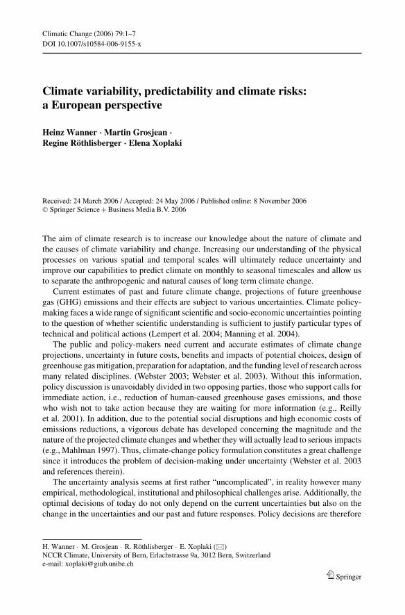
Contents
HEINZ WANNER, MARTIN GROSJEAN, REGINE ROTHLISBERGER andELENA XOPLAKI / Climate variability, predictability and climate risks: aEuropean perspective 1
CHRISTOPH C. RAIBLE, CARLO CASTY, JURG LUTERBACHER, ANDREASPAULING, JAN ESPER, DAVID C. FRANK, ULF BUNTGEN, ANDREASC. ROESCH, PETER TSCHUCK, MARTIN WILD, PIER-LUIGI VIDALE,CHRISTOPH SCHAR and HEINZ WANNER / Climate variability – observations,reconstructions, and model simulations for the Atlantic-European and Alpineregion from 1500–2100 AD 9
CORNELIA SCHWIERZ, CHRISTOF APPENZELLER, HUW C. DAVIES,MARK A. LINIGER, WOLFGANG MULLER, THOMAS F. STOCKER andMASAKAZU YOSHIMORI / Challenges posed by and approaches to the study ofseasonal-to-decadal climate variability 31
PIERLUIGI CALANCA, ANDREAS ROESCH, KARSTEN JASPER and MARTINWILD / Global warming and the summertime evapotranspiration regime of theAlpine region 65
J. FUHRER, M. BENISTON, A. FISCHLIN, CH. FREI, S. GOYETTE, K. JASPERand CH. PFISTER / Climate risks and their impact on agriculture and forests inSwitzerland 79
OLIVIER BAHN, LAURENT DROUET, NEIL R. EDWARDS, ALAIN HAURIE,RETO KNUTTI, SOCRATES KYPREOS, THOMAS F. STOCKER and JEAN-PHILIPPE VIAL / The coupling of optimal economic growth and climatedynamics 103
LAURENT VIGUIER, LEONARDO BARRETO, ALAIN HAURIE, SOCRATESKYPREOS and PETER RAFAJ / Modeling endogenous learning and imperfectcompetition effects in climate change economics 121
BEAT BURGENMEIER, ANDREA BARANZINI, CATHERINE FERRIER,CELINE GERMOND-DURET, KARIN INGOLD, SYLVAIN PERRET, PETERRAFAJ, SOCRATES KYPREOS and ALEXANDER WOKAUN / Economics ofclimate policy and collective decision making 143
Climatic Change (2006) 79:1–7DOI 10.1007/s10584-006-9155-x
Climate variability, predictability and climate risks:a European perspective
Heinz Wanner · Martin Grosjean ·Regine Rothlisberger · Elena Xoplaki
Received: 24 March 2006 / Accepted: 24 May 2006 / Published online: 8 November 2006C© Springer Science + Business Media B.V. 2006
The aim of climate research is to increase our knowledge about the nature of climate andthe causes of climate variability and change. Increasing our understanding of the physicalprocesses on various spatial and temporal scales will ultimately reduce uncertainty andimprove our capabilities to predict climate on monthly to seasonal timescales and allow usto separate the anthropogenic and natural causes of long term climate change.
Current estimates of past and future climate change, projections of future greenhousegas (GHG) emissions and their effects are subject to various uncertainties. Climate policy-making faces a wide range of significant scientific and socio-economic uncertainties pointingto the question of whether scientific understanding is sufficient to justify particular types oftechnical and political actions (Lempert et al. 2004; Manning et al. 2004).
The public and policy-makers need current and accurate estimates of climate changeprojections, uncertainty in future costs, benefits and impacts of potential choices, design ofgreenhouse gas mitigation, preparation for adaptation, and the funding level of research acrossmany related disciplines. (Webster 2003; Webster et al. 2003). Without this information,policy discussion is unavoidably divided in two opposing parties, those who support calls forimmediate action, i.e., reduction of human-caused greenhouse gases emissions, and thosewho wish not to take action because they are waiting for more information (e.g., Reillyet al. 2001). In addition, due to the potential social disruptions and high economic costs ofemissions reductions, a vigorous debate has developed concerning the magnitude and thenature of the projected climate changes and whether they will actually lead to serious impacts(e.g., Mahlman 1997). Thus, climate-change policy formulation constitutes a great challengesince it introduces the problem of decision-making under uncertainty (Webster et al. 2003and references therein).
The uncertainty analysis seems at first rather “uncomplicated”, in reality however manyempirical, methodological, institutional and philosophical challenges arise. Additionally, theoptimal decisions of today do not only depend on the current uncertainties but also on thechange in the uncertainties and our past and future responses. Policy decisions are therefore
H. Wanner · M. Grosjean · R. Rothlisberger · E. Xoplaki (�)NCCR Climate, University of Bern, Erlachstrasse 9a, 3012 Bern, Switzerlande-mail: [email protected]
Springer
2 Climatic Change (2006) 79:1–7
better modeled as sequential decisions under uncertainty (Hammitt et al. 1992; Manne andRichels 1995; Webster 2002). The sequential decision process adapts to new knowledge andresponds to new information and events. This flexible decision process requires a carefuladhesion to the uncertainties’ change whilst continuously integrating new knowledge onclimate system processes and socio-economic consequences and reactions (Webster 2003;Webster et al. 2003).
The quantification of uncertainty requires a model describing the fundamental and wellknown multi-sectoral (scientific as well as socio-economic) processes that contribute tothe results. Furthermore, the use of consistent and well-documented methods to developuncertainty estimates will allow the changes in our understanding to be tracked throughtime. In this case, a useful proportion of the uncertainties could be captured, although theparameters and assumptions of the model will still include some uncertainty (Webster 2003).Hence, a significant part of our uncertainty about past and future climate change will beunavoidable (Webster et al. 2003).
The importance of adequately quantifying and communicating uncertainty has been re-cently accepted in the climate research community. The authors for the Third AssessmentReport (TAR) of the Intergovernmental Panel on Climate Change (IPCC) were encouragedto quantify uncertainty as much as possible (Moss and Schneider 2000).
However, various limitations characterise these attempts to quantify uncertainty: (a)Climate observations were not used to constrain the uncertainty in climate model parameters(Wigley and Raper 2001). (b) By using only one Atmosphere-Ocean General CirculationModel (AOGCM), uncertainties in climate model response are reduced to uncertainty ina single scaling factor for optimizing the model’s agreement with observations (Stott andKettleborough 2002). (c) The IPCC emissions scenarios have been used as of equal like-lihood (Wigley and Raper 2001). (d) Some studies analysed the uncertainty only in theclimate system response without characterizing the economic uncertainty except through in-dividual IPCC emissions scenarios, by estimating uncertainty in future climate change onlyapplied to specific IPCC emissions scenarios (Allen et al. 2000; Knutti et al. 2002; Stott andKettleborough 2002). (e) The uncertainty analysis was in no case done under a policy scenarioleading to stabilisation of GHG concentrations. (f) Uncertainty estimates for reconstructionsof past climate (e.g., Mann et al. 1999; Luterbacher et al. 2004; Xoplaki et al. 2005) usuallydo not take into account dating uncertainty of the climate proxies (natural and documentary),loss of signal confidence within the twentieth century calibration period, uncertainties in theinstrumental data (e.g. Brohan et al. 2006 and references therein), assumptions about signalstationarity, proxies exhibiting an unquantified degradation in reliability, reduction of samplereplication, etc. (Esper et al. 2005).
Across all areas of climate change, it is found that uncertainty tends to increase whenmoving from global to regional scales. Regional information is clearly highly relevant topolicy, but generally is much less precise and can be ambiguous and confusing. Thus, acareful balance is needed when considering the scale at which policy relevant informationcan be provided (Manning et al. 2004). The assessment of potential regional impacts ofclimate change has, up to now, relied on data from coarse resolution AOGCMs, which donot resolve spatial scales of less than ∼300 km (Mearns et al. 2001).
According to Dessai and Hulme (2004) there are two different sources of uncertainty, the“epistemic” and the “stochastic”. Epistemic uncertainty originates from incomplete knowl-edge of processes that influence events. These sources of uncertainty can be reduced by furtherstudying the climate system, improving the state of knowledge, etc. Stochastic sources of un-certainty are those that are considered “unknowable” knowledge – items such as variability inthe system, the chaotic nature of the climate system, and the indeterminacy of human systems
Springer
Climatic Change (2006) 79:1–7 3
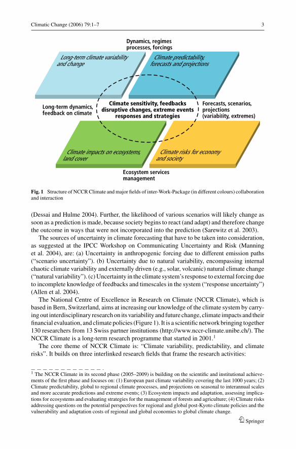
Fig. 1 Structure of NCCR Climate and major fields of inter-Work-Package (in different colours) collaborationand interaction
(Dessai and Hulme 2004). Further, the likelihood of various scenarios will likely change assoon as a prediction is made, because society begins to react (and adapt) and therefore changethe outcome in ways that were not incorporated into the prediction (Sarewitz et al. 2003).
The sources of uncertainty in climate forecasting that have to be taken into consideration,as suggested at the IPCC Workshop on Communicating Uncertainty and Risk (Manninget al. 2004), are: (a) Uncertainty in anthropogenic forcing due to different emission paths(“scenario uncertainty”). (b) Uncertainty due to natural variability, encompassing internalchaotic climate variability and externally driven (e.g., solar, volcanic) natural climate change(“natural variability”). (c) Uncertainty in the climate system’s response to external forcing dueto incomplete knowledge of feedbacks and timescales in the system (“response uncertainty”)(Allen et al. 2004).
The National Centre of Excellence in Research on Climate (NCCR Climate), which isbased in Bern, Switzerland, aims at increasing our knowledge of the climate system by carry-ing out interdisciplinary research on its variability and future change, climate impacts and theirfinancial evaluation, and climate policies (Figure 1). It is a scientific network bringing together130 researchers from 13 Swiss partner institutions (http://www.nccr-climate.unibe.ch/). TheNCCR Climate is a long-term research programme that started in 2001.1
The core theme of NCCR Climate is: “Climate variability, predictability, and climaterisks”. It builds on three interlinked research fields that frame the research activities:
1 The NCCR Climate in its second phase (2005–2009) is building on the scientific and institutional achieve-ments of the first phase and focuses on: (1) European past climate variability covering the last 1000 years; (2)Climate predictability, global to regional climate processes, and projections on seasonal to interannual scalesand more accurate predictions and extreme events; (3) Ecosystem impacts and adaptation, assessing implica-tions for ecosystems and evaluating strategies for the management of forests and agriculture; (4) Climate risksaddressing questions on the potential perspectives for regional and global post-Kyoto climate policies and thevulnerability and adaptation costs of regional and global economies to global climate change.
Springer
4 Climatic Change (2006) 79:1–7
1. What is the nature of past, current and future climate? What is the sensitivity of theclimate system (including the internal variations and extremes) to anthropogenic andnatural perturbations? What are the feedbacks between the atmosphere, the ocean, thecryosphere, land surfaces and the anthroposphere?
2. What are the forced climate impacts on ecosystems, economy and society? What is thelikelihood of rapid transitions and changes with disruptive impacts? What is the role ofextreme climate events on ecosystems, the economy and society?
3. What are the options and strategies for the management of ecosystems, economic systemsand societal systems to respond to such climate changes and to reduce vulnerability?
Within the structure of the NCCR climate research, there are three geographical scales(Switzerland including the greater Alpine area, Europe and global) and three temporal scales(the last 500 years, the present and the 21st century).
The issues targeted in NCCR Climate require work at a wide range of spatial and temporalscales as well as the combination and integration of results from observational, experimentaland modelling studies. Developing methodologies and providing an environment to workacross the boundaries of different scales and methods is a priority area in climate research. Itis intellectually and technically challenging, but a prerequisite to address the complex natureof the research issues in an adequate manner.
This book (special issue) compiles seven consecutive and integrative chapters, which (i)address some of the aforementioned common scientific challenges in current climate andclimate impact research and (ii) synthesize the interdisciplinary research across the largethematic umbrella of the NCCR Climate. The scientific voyage starts with two selectedproblems of atmospheric and climate research, that address (i) different scales in time fromthe past to the future with different types of data availability (Raible et al. 2006), and (ii)reducing uncertainty of climate predictions and projections (Schwierz et al. 2006). We thenmove on to the topic of future climate change impacts on natural and managed ecosystems.The main challenge of climate impacts research is to consolidate the large scale projectionsto regional or local scales of climate variability and change, which can then be integratedinto more specialised climate impact models (Calanca et al. 2006). Impacts are not limitedto ecosystems but encompass the entire social, technological and economic systems (Fuhreret al. 2006). Thus, building a modelling framework where the climate system and the energy-economy-environment systems communicate interactively with each other (Bahn et al. 2006)is fundamental in order to assess future development paths, strategies and options for climatechange mitigation policies (Viguier et al. 2006). Finally, it is the society, at different hierar-chical levels with different organizational forms and institutions, which makes the decisionsand assesses the future failure or success of any climate change policy (Burgenmeier et al.2006).
Raible et al. (2006) assessed the natural climate variability on interannual to decadaltimescales by using AOGCMs, state-of-the-art regional circulation models in combinationwith multiproxy climate reconstructions from regional to continental scales. The reconstruc-tions reveal pronounced interdecadal variations, which seem to “lock” the atmospheric cir-culation in quasi-steady long-term patterns over multi-decadal periods, which partly controlthe continental alpine temperature and precipitation variability. In contrast, the climate modelsimulations indicate some substantial differences to the observations, indicating that the tele-connectivity between modeled climate variables is weaker than in observations however, inthe future these teleconnections seem to be more stable. This partial disagreement betweenthe reconstructions and the model simulations implies the need for better instrumental andmore numerous natural/documentary proxy data sets, further improvement in reconstruction
Springer
Climatic Change (2006) 79:1–7 5
methods and multi-model ensemble approaches (combination of regional and global models)(e.g., Yoshimori et al. 2005; Goosse et al. 2005, 2006; Raible et al. 2006).
Today’s climate models capture the essence of the large-scale aspects of the current climateand its considerable natural variability reasonably well on time scales ranging from oneday to decades. Despite this significant achievement, the models show weaknesses that adduncertainty to the very best model projections of human-induced climate changes.
Schwierz et al. (2006) present an overview of the uncertainties in climate model projectionsthat arise from various sources. They identified uncertainties stemming from the complexityand non-linearity of the climate system, its irregular evolution and the changing climatesensitivity, the emission scenarios selection and their implications for the radiative forcing,and the inevitably incomplete and inadequate representation of the climate system in a weatheror climate model. The latter uncertainty can be separated into that which is connected with themodel equations representing the climate system interactions, the limited representation ofphysical processes due to the low resolution of the models and the limited knowledge of somephysical processes including the non-linear interactions between the climate components.Schwierz et al. (2006) report that a hierarchy of models is a powerful approach to estimate andassess uncertainty, while the combination of different kinds of models of different complexitywith an overlap between the model evaluations can contribute to the quantification andreduction of uncertainties from future climate model projections.
Calanca et al. (2006) combined simulations with a state-of-the-art Global CirculationModel (GCM) complemented by an experiment with a high-resolution spatially distributedhydrological model in order to quantify the impact of climate change and to reveal regionaldifferences in the response, both across the alpine region as well as within individual riverbasins in Switzerland. They found that GCMs alone cannot capture the detailed regional scaleresults, demonstrating the danger of a simple extrapolation of GCM results and underliningthe importance of a highly resolved hydrological model for the quantitative assessment ofthe regional impacts of climate change. Current spatial resolution of GCMs is too coarse toadequately represent areas of complex topography and land use change (Calanca et al. 2006).
Fuhrer et al. (2006) assessed climate risks on ecosystems using simulations for presentclimate with a 50-km Regional Climate Model (RCM) with boundary conditions from aGCM control experiment and compared the model output with observations. Climate risksarise from complex interactions between climate, environment, social and economic systems.They represent combinations of the likelihood of climate events and their consequences forsociety and the environment. The assessment of climate risks depends on both the ability tosimulate extreme events in various scales and the understanding of the responses of the targetsystem. The projections of climate risks are dependant on the quality of the link betweenlarger-scale climate simulations and small-scale effects. Extreme climate events are oftenrelated to large-scale synoptic conditions, but the scales at which impacts occur can varyfrom local to regional (Fuhrer et al. 2006).
In order to obtain an integrated assessment of climate policies, Bahn et al. (2006) estab-lished a two-way coupling between the economic module of a well-established integratedassessment model and an intermediate complexity “3-D” climate model. The coupling isachieved through the implementation of an advanced “oracle based optimisation technique”which permits the integration of information coming from the climate model during thesearch for the optimal economic growth path. They showed that further applications of thismethod could include the coupling of an economic model and an advanced climate modelthat could describe the carbon cycle. Additionally, the spatial resolution of the climate modelallows the construction of regional damage functions or in other words, the ability to linkclimate feedbacks with economic activity (e.g. agriculture). A further step is the coupling of
Springer
6 Climatic Change (2006) 79:1–7
a macro-economic growth module with a detailed techno-economic model, in addition to thecoupling with a moderate complexity climate model (Bahn et al. 2006).
Viguier et al. (2006) used an optimal economic growth model, a multi-region bottom-upprocess model and a multi-region computable general economic equilibrium (CGE) modelfor the assessment of climate change policies. Their assessment reveals the important effectof endogenising technological learning by early investments in research and development(R&D) activities and demonstration and deployment (D&D) programs. These programs couldsupport the development and diffusion of cleaner technologies in the long term, and influencethe strategic behaviour of climate policy makers and ultimately the success of internationalclimate-policy. The strategic behaviour of the different countries towards the Kyoto protocolis related with the connected costs and the ability of the governments to afford these costs.
Burgenmeier et al. (2006) explore the reasons behind the reluctant application of economicinstruments of climate change. They stress the need for interdisciplinary research linkingeconomic theory and empirical testing to deliberative political procedures. They found thatthe promotion of economic policies of climate change has to be completed by social policiesto capture the ethical aspects. Additionally, the problem of the social acceptance of economicinstruments of climate change can be overcome by using a) Conventional models that considerthe environment, either through public goods theory or through property rights theory andb) More global models featuring relationships between economics, the biosphere and socialaspects in order to come closer to the concept of sustainable development.
The understanding of the likelihood of future climate requires further and repeated analysisof the up-to-date combined knowledge on the climate and socio-economic systems (Websteret al. 2003).
Acknowledgements The NCCR Climate is supported by the Swiss National Science Foundation. We wouldlike to thank Prof. George Zaimes from the School of Natural Sciences at the University of Arizona for hisconstructive comments on the document, Dr. Paul Della-Marta from the Institute of Geography at the Universityof Bern for proofreading the English text and Mr. Andreas Brodbeck from the Institute of Geography at theUniversity of Bern, for drawing the figure.
References
Allen MR, Booth BBB, Frame DJ, Gregory JM, Kettleborough JA, Smith LA, Stainforth DA, Stott PA (2004)Observational constraints on future climate: distinguishing robust from model-dependent statements ofuncertainty in climate forecasting. In: Manning et al. (eds) Describing scientific uncertainties in climatechange to support analysis of risk and of options May 2004 IPCC workshop report. IPCC Working GroupI Technical Support Unit, Boulder, Colorado, USA, pp 53–57(Available at: http://www.ipcc.ch/)
Allen MR, Stott PA, Mitchell JFB, Schnur R, Delworth TL (2000) Quantifying the uncertainty in forecasts ofanthropogenic climate change. Nature 407:617–620
Bahn O, Drouet L, Edwards NR, Haurie A, Knutti R, Kypreos S, Stocker TF, Vial JP (2006) The coupling ofoptimal economic growth and climate dynamics. Clim Change, DOI: 10.1007/s10584-006-9108-4 (thisissue)
Brohan P, Kennedy JJ, Harris I, Tett SFB, Jones PD (2006) Uncertainty estimates in regional and globalobserved temperature changes: a new dataset from 1850. J Geophys Res DOI: 10.1029/2005JD00654
Burgenmeier B, Baranzini A, Ferrier C, Germond-Duret C, Ingold K, Perret S, Rafaj P, Kypreos S, Wokaun A(2006) Economics of climate policy and collective decision making. Clim Change, DOI: 10.1007/s10584-006-9147-x (this issue)
Calanca P, Roesch A, Jasper K, Wild M (2006) Global warming and the summertime evapotranspirationregime of the alpine region. Clim Change, DOI: 10.1007/s10584-006-9103-9 (this issue)
Dessai S, Hulme M (2004) Does climate adaptation policy need probabilities? Climate Policy 4:107–128Esper J, Wilson RJS, Frank DC, Moberg A, Wanner H, Luterbacher J (2005) Climate: past ranges and future
changes. Quat Sci Rev 24:2164–2166
Springer
Climatic Change (2006) 79:1–7 7
Fuhrer J, Beniston M, Fischlin A, Frei C, Goyette S, Jasper K, Pfister C (2006) Climate risks and their impacton agriculture and forests in switzerland. Clim Change, DOI: 10.1007/s10584-006-9106-6 (this issue)
Goosse H, Renssen H, Timmermann A, Bradley RS (2005) Natural and forced climate variability during thelast millennium: A model-data comparison using ensemble simulations Quat Sci Rev 24:1345–1360
Goosse H, Renssen H, Timmermann A, Bradley RS, Mann ME (2006) Using paleoclimate proxy-data to selectand optimal realisation in an ensemble of simulations of the climate of the past millennium Clim Dynam..DOI: 10.1007/s00382-006-0128-6, 27:165–184
Hammit JK, Lempert RJ, Schlesinger ME (1992) A sequential-decision strategy for abating climate change.Nature 357:315–318
Knutti R, Stocker TF, Joos F, Plattner GK (2002) Constraints on radiative forcing and future climate changefrom observations and climate model ensembles. Nature 416:719–723
Lempert R, Nakicenovic N, Sarewitz D, Schlesinger ME (2004) Characterizing climate-change uncertaintiesfor decision-makers. Clim Change 65:1–9
Luterbacher J, Dietrich D, Xoplaki E, Grosjean M, Wanner H (2004) European seasonal and annual temperaturevariability, trends, and extremes since 1500. Science 303:1499–1503
Mahlman JD (1997) Uncertainties in projections of human-caused climate warming. Science 278:1416–1417Mann ME, Bradley RS, Hughes MK (1999) Northern hemisphere temperatures during the past millennium:
inferences, uncertainties, and limitations. Geophys Res Lett 26:759–762Manne AS, Richels RG (1995) The greenhouse debate: economic efficiency, burden sharing and hedging
strategies. Energy J 16:1–37Manning et al. (eds.) (2004) Describing scientific uncertainties in climate change to support analysis of risk
and of options, may 2004 ipcc workshop report. IPCC Working Group I Technical Support Unit, Boulder,Colorado, USA, pp 138. (Available at: http://www.ipcc.ch/)
Mearns LO, Hulme M, Carter TR, Leemans R, Lal M, Whetton PH (2001) Climate scenario development.Chapter 13 In: Houghton J, et al. (eds), Clim Change 2001: The Scientific Basis, Intergovernmental Panelon Climate Change, Cambridge University Press, pp 739–768
Moss RH, Schneider SH (2000) In: Pachauri R, Taniguchi T, Tanaka K (eds), Guidance papers on the crosscutting issues of the third assessment report. World Meteorological Organization, Geneva, pp 33–57
Raible CC, Casty C, Luterbacher J, Pauling A, Esper J, Frank DC, Buntgen U, Roesch AC, Tschuck P,Wild M, Vidale PL, Schar C, Wanner H (2006) Climate variability – observations, reconstructions, andmodel simulations for the atlantic-european and alpine region from 1500–2100 AD. Clim Change, DOI:10.1007/s10584-006-9061-2 (this issue)
Reilly J, Stone PH, Forest CE, Webster MD, Jacoby HD, Prinn RG (2001) Climate change: uncertainty andclimate change assessments. Science 293:430–433
Sarewitz D, Pielke RA Jr., Keykhah M (2003) Vulnerability and risk: some thoughts from a political and policyperspective. Risk Analysis 23:805–810
Schwierz C, Appenzeller C, Davies HC, Liniger MA, Muller W, Stocker TF, Yoshimori M (2006) Challengesposed by and approaches to the study of seasonal-to-decadal climate variability. Clim Change, DOI:10.1007/s10584-006-9076-8 (this issue)
Stott P, Kettleborough JA (2002) Origins and estimates of uncertainty in predictions of twenty-first centurytemperature rise. Nature 416:723–726
Viguier L, Barreto L, Haurie A, Kypreos S, Rafaj P (2006) Modeling endogenous learning and imperfectcompetition effects in climate change economics. Clim Change, DOI: 10.1007/s10584-006-9070-1 (thisissue)
Webster M (2002) The curious role of learning in climate policy: should we wait for more data? Energy J23:97–119
Webster M (2003) Communicating climate change uncertainty to policy-makers and the public. Clim Change61:1–8
Webster M, Forest C, Reilly J, Babiker M, Kicklighter D, Mayer M, Prinn R, Sarofim M, Sokolov A, Stone P,Wang C (2003) Uncertainty analysis of climate change and policy response. Clim Change 61:295–320
Wigley TML, Raper SCB (2001) Interpretations of high projections for global-mean warming. Science293:451–454
Xoplaki E, Luterbacher J, Paeth H, Dietrich D, Steiner N, Grosjean M, Wanner H (2005) European springand autumn land temperatures, variability and change of extremes over the last half millennium. GeophysRes Lett 32:L15713
Yoshimori M, Stocker TF, Raible CC, Renold M (2005) Externally-forced and internal variability in ensembleclimate simulations of the Maunder Minimum. J Climate 18:4253–4270
Springer
Climatic Change (2006) 79:9–29DOI 10.1007/s10584-006-9061-2
Climate variability – observations, reconstructions, andmodel simulations for the Atlantic-European and Alpineregion from 1500–2100 AD
Christoph C. Raible · Carlo Casty · Jurg Luterbacher ·Andreas Pauling · Jan Esper · David C. Frank ·Ulf Buntgen · Andreas C. Roesch · Peter Tschuck ·Martin Wild · Pier-Luigi Vidale · Christoph Schar ·Heinz Wanner
Received: 18 October 2004 / Accepted: 9 November 2005 / Published online: 1 November 2006C© Springer Science + Business Media B.V. 2006
Abstract A detailed analysis is undertaken of the Atlantic-European climate using data from500-year-long proxy-based climate reconstructions, a long climate simulation with perpetual1990 forcing, as well as two global and one regional climate change scenarios. The observedand simulated interannual variability and teleconnectivity are compared and interpreted inorder to improve the understanding of natural climate variability on interannual to decadaltime scales for the late Holocene. The focus is set on the Atlantic-European and Alpine re-gions during the winter and summer seasons, using temperature, precipitation, and 500 hPageopotential height fields. The climate reconstruction shows pronounced interdecadal vari-ations that appear to “lock” the atmospheric circulation in quasi-steady long-term patternsover multi-decadal periods controlling at least part of the temperature and precipitation vari-ability. Different circulation patterns are persistent over several decades for the period 1500to 1900. The 500-year-long simulation with perpetual 1990 forcing shows some substantialdifferences, with a more unsteady teleconnectivity behaviour. Two global scenario simula-tions indicate a transition towards more stable teleconnectivity for the next 100 years. Timeseries of reconstructed and simulated temperature and precipitation over the Alpine regionshow comparatively small changes in interannual variability within the time frame consid-ered, with the exception of the summer season, where a substantial increase in interannualvariability is simulated by regional climate models.
C. C. RaibleClimate and Environmental Physics, Physics Institute, University of Bern, Sidlerstrasse 5, CH-3012Bern, Switzerland
C. Casty · J. Luterbacher · A. Pauling · H. WannerInstitute of Geography, University of Bern, Hallerstrasse 12, CH-3012 Bern, Switzerland
J. Esper · D. C. Frank · U. BuntgenSwiss Federal Research Institute WSL, Zurcherstrasse 111, CH-8903 Birmensdorf, Switzerland
A. C. Roesch · P. Tschuck · M. Wild · P.-L. Vidale · C. ScharInstitute for Atmospheric and Climate Science ETH, Winterthurerstrasse 190, CH-8057 Zurich,Switzerland
Springer
10 Climatic Change (2006) 79:9–29
1 Introduction
Observations and reconstructions for the late Holocene show that the warming since the1960s is likely unprecedented over the last millennium (Jones and Mann 2004). Modellingstudies give some evidence that the temperature change of at least the second half of the20th century can only be explained by including anthropogenic forcing (Rind et al. 1999;Crowley 2000; IPCC 2001; Meehl et al. 2003; Bauer et al. 2003). Nevertheless, to assessfuture climate change for key regions, like the Atlantic-European area, with confidence,a thorough understanding of the underlying mechanisms of natural climate variability ondifferent spatio-temporal scales for the late Holocene is necessary (Jones and Mann 2004).
One possibility to address the understanding of natural climate variability of the Atlantic-European region is to investigate general circulation models (GCMs). Modelling results showthat for the mid-latitudes the coupling between atmosphere and ocean plays a major role ondecadal variability (Grotzner et al. 1998; Raible et al. 2001; Marshall et al. 2001, and refer-ences therein). This coupling has implications for the low-frequency (decadal) behaviour ofthe North Atlantic Oscillation (NAO), with its well-known linkage to temperature and pre-cipitation on the interannual time scale (Hurrell 1995; Hurrell and Loon 1997; Wanner et al.2001; Hurrell et al. 2003). Even baroclinic high-frequency variations characterised by station-ary and transient wave activity should be incorporated to understand enhanced low-frequencyvariability of the NAO (Raible et al. 2004). Additionally, future projections integrated withcoupled atmosphere-ocean (AO-) GCMs show a systematic northeastward shift of the north-ern center of action of the NAO (Ulbrich and Christoph 1999), indicating that at least themodelled position of the pressure centers is not stable in time. Recently, a strong connectionbetween sea surface temperature (SST) and the North Atlantic Thermohaline Circulation hasbeen presented in unforced control AO-GCM simulations (Latif et al. 2004; Cheng et al.2004). These SST anomalies, containing strong multi-decadal variability, may mask anthro-pogenic signals in the North Atlantic region. Another potential mechanism of generatinglow-frequency NAO variability is the stratosphere, where stratospheric processes can be in-fluenced by changes in the external solar and volcanic forcing (Shindell et al. 2001, 2003).Another problem present in this region is illustrated by an ensemble modelling study for theMaunder Minimum from 1640 to 1715 (Yoshimori et al. 2005), showing that forcing signals,e.g., solar forcing, are difficult to detect due to the strong internal variability induced by theNAO.
Another approach to improve our understanding of natural climate variability is to extendthe existing climate records for temperature, precipitation, and atmospheric circulation pat-terns back in time. One first step was to reconstruct temperature on hemispheric to globalscales over the past centuries to millennia based on empirical proxy data (Bradley and Jones1993; Overpeck et al. 1997; Jones et al. 1998; Mann et al. 1998; Briffa et al. 2001; Esperet al. 2002a; Cook et al. 2004; Jones and Mann 2004; Esper et al. 2004; Moberg et al. 2005).However, hemispheric-scale reconstructions provide little information about regional scaleclimate variability. Therefore, studies focusing on reconstruction of specific regions, e.g.,Atlantic-Europe or high Asia, utilising documentary (Luterbacher et al. 2004; Xoplaki et al.2005; Guiot et al. 2005) and tree-ring data (Esper 2000; Esper et al. 2002b, 2003; Buntgenet al. 2005) are also valuable.
Jones et al. (2003) found amongst others changes in the annual cycle of Northern Hemi-sphere temperatures indicating that, compared with earlier times, winters have warmed morerelative to summers over the past 200 years.
A third research focus is on atmospheric circulation variability. Besides traditional re-constructions of the NAO index (Appenzeller et al. 1998; Luterbacher et al. 2002a; Cook
Springer
Climatic Change (2006) 79:9–29 11
et al. 2002; Vinther et al. 2003), atmospheric circulation modes (Jacobeit et al. 2003) for eachmonth in the year were derived from sea-level pressure field reconstructions (Luterbacheret al. 1999, 2002b). Utilising reconstructions of the 500 hPa geopotential height fields forthe Atlantic-European region, Casty et al. (2005a) found that climate regimes, defined by thejoint probability density function of the first two leading Empirical Orthogonal Functions,are not stable in time.
With a steadily growing data base, it is now possible to reconstruct climate variations fromsmall regions like the European Alps (Casty et al. 2005b; Frank and Esper 2005; Buntgenet al. 2005). This could help to place extreme events, e.g., the hot European summer of 2003(with its maximum deviation from the mean in central Europe and the Alps), in a longer-termcontext (Luterbacher et al. 2004). Recently, regional modelling studies (Schar et al. 2004)showed that in a scenario with increased atmospheric greenhouse-gas concentrations, futureEuropean temperature variability may increase by up to 100%, with maximum changes incentral and eastern Europe. Such a change in variability would have a strong impact on notonly the environment, but also on the society and the economy in these regions.
The National Center of Competence in Research on Climate (NCCR Climate) in Switzer-land provides a substantial variety of different spatio-temporal highly-resolved climate infor-mation, ranging from natural and documentary proxy reconstructions, to high-quality instru-mental measurements, to modeled data from state-of-the-art general circulation and regionalmodels for both present day climate conditions (fixed to 1990 AD) as well as future scenarios.The aim of this study is to combine the two major types of information in the archive – theobservations and reconstructions on the one hand, and the simulations for present day climateconditions and future scenarios on the other hand. This set of data and simulations will formthe basis for the investigation of the atmospheric circulation and its links to the behaviour oftemperature and precipitation in the Atlantic-European and the Alpine regions on interannualto decadal time scales. Additionally, changes in the annual cycle from 1500–2100 AD arediscussed.
The outline of this paper is as follows: In Section 2 the reconstructed and modeled data,as well as some analysis techniques and definitions, are introduced. Subsequent analysisconcentrates on the Atlantic-European (Section 3) and Alpine (Section 4) regions, illustratingthe relationship between large-scale flow regimes and temperature and precipitation. Theresults are summarised and interpreted, in the context of published evidence, in Section 5.
2 Reconstructions, models, and analysis techniques
The study is based on a set of reconstructed and modeled data, which is introduced as follows.We focus on winter (December to February, DJF) and summer (June to August, JJA) of theAtlantic-European and the Alpine regions, respectively.
2.1 Reconstructions and models
Reconstructions of past pressure, temperature, and precipitation are performed through mul-tivariate statistical climate fields reconstruction (CFR) approaches. CFR seeks to reconstructa large-scale field by regressing a spatial network of proxy indicators (e.g., early instrumen-tal, tree-ring data, and historical evidences) against instrumental field information (Jones andMann 2004). During periods when both proxy and instrumental field information (reanaly-ses) are available, regression models are developed and fed with proxy data to reconstructpast climate variables.
Springer
12 Climatic Change (2006) 79:9–29
For the Atlantic-European region reconstructions of seasonally resolved land surface airtemperature (Luterbacher et al. 2004, 25◦W–40◦E and 35◦N–70◦N), precipitation (Paul-ing et al. 2006, 10◦W–40◦E and 35◦N–70◦N), and 500 hPa geopotential height fields(Luterbacher et al. 2002b, 30◦W–40◦E and 30◦N–70◦N) are available back to 1500. In-dependent reconstructions, i.e., sharing no common predictors, have been developed forseasonal land surface air temperatures and precipitation fields for the European Alps since1500 (Casty et al. 2005b, 4◦E–16◦E and 43◦N–48◦N). These CFRs are multi-proxy based.The period from 1500 to the late 17th century comprises entirely documentary and naturalproxies; the period from 1659 to around 1750 includes a mix of documentary, natural proxiesas well as a few early instrumental data. The reconstructions for the last 250 years are entirelybased on instrumental time series, the number of those increasing steadily over time. A com-pilation of all proxies and instrumental data used for those 500 year climate reconstructionsis given in Luterbacher et al. (2004), Casty et al. (2005b), and Pauling et al. (2006). Thespatial resolution for the temperature and precipitation reconstructions is 0.5◦ (∼60 km ×60 km) similar to the instrumental field information for the 1901–2000 period: Instrumentaldata from New et al. (2000) were used by Luterbacher et al. (2004); data from Mitchell et al.(2004) were used by Casty et al. (2005b) and Pauling et al. (2006). The 500 hPa fields areresolved on a 2.5◦ grid similar to the NCEP Reanalysis data (Kalnay et al. 1996; Kistler et al.2001). For further details about reconstruction methods, proxy information, verification, anduncertainty estimates, the reader is referred to Luterbacher et al. (2002b, 2004), Casty et al.(2005b), and Pauling et al. (2006).
A new millennial-long tree-ring reconstruction utilising 1527 ring width measurementseries from living and relict larch and pine samples from the Swiss and Austrian Alps (46.5◦N–47◦N and 7.5◦N–11.5◦E) is applied for further comparison and validation (Buntgen et al.2005). This record was detrended using the Regional Curve Standardisation (RCS) method(Briffa et al. 1992), and calibrated and verified against high elevation station temperature data(Bohm et al. 2001) over the 1864–2002 period. Note that this reconstruction is independentfrom Casty et al. (2005b).
Two different ocean-atmosphere general circulation models (OA-GCMs) are used in thisstudy. The first model is the Max Planck Institute for Meteorology global coupled model,ECHAM5/MPI-OM. The resolution of the atmospheric component, ECHAM5 (Roeckneret al. 2003, version 5.0), is 19 levels in the vertical dimension and T42 in spectral space,which corresponds to a horizontal resolution of about 2.8◦ × 2.8◦. The oceanic component,MPI-OM (Marsland et al. 2003), is based on a Arakawa C-grid (Arakawa and Lamb 1981)version of the HOPE ocean model (Wolff et al. 1997). It is run on a curvilinear grid withequatorial refinement and includes 20 vertical levels. A dynamic/thermodynamic sea icemodel (Marsland et al. 2003) and a hydrological discharge model (Hagemann and Duemenil-Gates 2001) are included. The atmospheric and oceanic components are connected with theOASIS coupler (Terray et al. 1998). The model does not employ flux adjustment or any othercorrections. Initial ocean conditions are taken from a 500-yr control integration. The model isforced from stable conditions with a 1% CO2 increase per year from 1990 (348 ppm) to 2100(1039 ppm). Hereafter, this experiment is denoted as ECHAM5 1% CO2. This forcing is acommonly used scenario to intercompare the sensitivity of different coupled climate modelsto increased greenhouse gases.
The second setup is the Climate Community System Model (CCSM), version 2.0.1,1
developed by the National Center for Atmospheric Research (NCAR) (Kiehl et al. 1998;
1 http://www.ccsm.ucar.edu/models/
Springer
Climatic Change (2006) 79:9–29 13
Blackmon et al. 2001). The atmospheric part of this coupled model has a horizontal resolutionof T31 (∼3.75◦ × 3.75◦) with 26 vertical levels; the ocean component has ∼3.6◦ × 1.8◦
resolution with 25 levels. The CCSM also runs without any flux corrections. Two simulationswere carried out: a 550-yr simulation for constant present day climate conditions fixed to1990 AD (denoted as CCSM 1990) and a 1% CO2 simulation (denoted as CCSM 1% CO2)starting from the stable state of the CCSM 1990 (Raible et al. 2005). Note that for the CCSM1990, the first 50 years are ignored until the model adjusts to its stable climate state. TheCCSM is integrated on two different computer platforms, an IBM SP4 and a Linux cluster(Renold et al. 2004). Note that the different computer platforms have no influence on themean behaviour of the simulations.
Regionally, we use the Climate High Resolution Model (CHRM) which is driven by theHadley Center HadAM3 atmospheric GCM at the lateral boundary (Pope et al. 2000). TheCHRM regional model covers Europe and a fraction of the North Atlantic on a 81 by 91grid point domain with a resolution of approximately 56 km and a time step of 300 s (seeVidale et al., 2003 for model set-up). The CHRM has been validated regarding its ability torepresent natural interannual variations (Vidale et al. 2003) and the precipitation distributionin the Alpine region (Frei et al. 2003) using a simulation that is driven by the ECMWFreanalysis ERA-15 (Gibson et al. 1999). Two time-slice simulations are performed: Forthe control simulation from 1961–1990 the HadAM3 and the nested CHRM uses observedSSTs and observed greenhouse gas concentrations. The second experiment for the time-slice 2071–2100 uses the forcing of an IPCC A2 scenario (IPCC 2001). To assure thatchanges in variability between the two simulations are not associated to SST changes, butare due to the atmospheric models and their interaction with the land surface, the so-calleddelta change approach is applied to the experimental setup (Jones et al. 2001). Both GCMHadAM3 simulations, delivering the boundary conditions for the CHRM regional model, usethe same SST variations (taken from the 1960–1990 observations), but a mean SST warmingis added to the A2 scenario simulations by using the warming signal from the coupled HadCMsimulation. Both simulations have a one year spin-up phase: 1960 and 2070, respectively.
2.2 Analysis techniques
The analysis presented in this paper is restricted to the Atlantic-European and the Alpineregion. Time series are defined for both regions. The temperature time series is the mean over25◦W–40◦E and 35◦N–70◦N for the European land area and over 4–16◦E and 43–48◦N forthe Alpine region. For the precipitation time series the Atlantic-European region was reducedto 10◦W–30◦E and 35◦N–70◦N due to the smaller area available from the reconstructions(Pauling et al. 2006). To emphasise and extract low-frequency variability, a 31-yr triangularfilter was applied. The first and the last 15 years of the time series are not analysed to avoidedge effect problems.
To merge the time series from climate simulations and reconstructions, and to account forbiases of the model simulations, anomalies with respect to the overlapping 1990–2000 and1961–1990 periods were used for the Atlantic-European and the Alpine area, respectively.Biases between the model output and the reconstructions are amongst others due to the coarsemodel resolution (horizontally and vertically) and the inclusion of sea areas which are notconsidered in the reconstructions. Moreover, due to the different horizontal resolution thesize of the area slightly varies from the reconstructions. Other reasons for biases could also bethe uncertainties of the proxy input data of the reconstruction method as well as systematicmodel errors, e.g., model drifts and underestimation of subgrid scale variability. Filtering
Springer
14 Climatic Change (2006) 79:9–29
-0.9 -0.8 -0.7 -0.6 -0.5
340˚ 0˚ 20˚ 40˚30˚
40˚
50˚
60˚
70˚
Fig. 1 An example of a 30-yr window (1973–2002), where the teleconnectivity of the 500 hPa geopotentialheight (DJF, shaded) and the corresponding axis of teleconnectivity (red line) is denoted
was applied to each time series separately in order to avoid mixing model and reconstructiondata. However, this results in gaps in the filtered time series.
The spatio-temporal behaviour of the circulation of the free atmosphere can be charac-terised by the teleconnectivity of the 500 hPa geopotential height. According to Wallace andGutzler (1981) the teleconnectivity is defined as the strongest negative correlation of onebase point with all grid points assigned at the base point. As base point, all grid points areiteratively chosen. Only strong negative correlations which cluster together in a large areaare considered as “centers of action”. Thus, anticorrelated centers of action, e.g., the NAOwith its poles near Iceland and the Azores, are easily identified. To find the center that isanticorrelated with another one, a search algorithm is applied to the teleconnectivity map. Ina 20◦ × 10◦ longitude/latitude neighbourhood the strongest negative correlation coefficientis identified. Provided that the region is large enough to capture one center of action, thesize of search area is not a critical factor in this procedure. Then, this grid point is againcorrelated with all others in the 500 hPa geopotential height providing the position of thegrid point which has the strongest negative correlation. These positions are connected withlines denoting the axis of the opposing centers of action. In order to illustrate this method,Figure 1 shows the teleconnectivity of the reconstructed 500 hPa geopotential height (shad-ings) in winter (DJF) and the axis of the anticorrelated centers of action (red line) for the1973 to 2002 period. The two centers of action are easily identified. Perpendicular to theaxis, the atmospheric flow is strengthened or weakened, depending on the sign of the centersof action. For example, if the northern center is negative and the southern is positive, thewesterly atmospheric flow is stronger than average, and vice versa.
The technique was applied to the 500 hPa geopotential height data for a 30-yr runningwindow, where only the axes of the conversing centers of action are displayed. This resultsin a three-dimensional Hovmoller diagram (e.g., Figure 5) which shows the spatio-temporalbehaviour of atmospheric circulation patterns. The window size was chosen to fit to the filterapplied to the time series and also to correspond to the window regularly used for time-sliceexperiments with highly resolved climate models in the climate change community (Wild
Springer
Climatic Change (2006) 79:9–29 15
et al. 2003). Another reason for setting the size to 30 years is that the World Meteorolog-ical Organisation defines climatological mean to be a 30-yr mean. Nevertheless, tests withmoderate changes of the window size, e.g., 40 years, confirm the results in the followingsections.
3 Climate variability in the Atlantic-European area
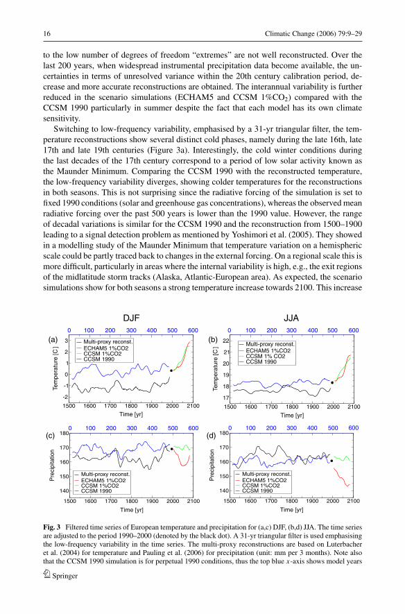
To investigate climate variability in the Atlantic-European region we first focus on the re-constructed time series. The interannual variation of the temperature reconstruction (Luter-bacher et al. 2004, Figure 2a,b) shows larger variability in winter (standard deviation of1.1 ◦C) than in summer (standard deviation of 0.44 ◦C). This is in contrast to the threesimulations, showing a standard deviation of about 0.65 ◦C in winter and 0.4 ◦C in sum-mer, and illustrating a model deficiency in winter and/or the difference calculating theaverages for different resolution. Comparing the CCSM 1990 simulation with the twoscenario simulations, the variability on this time scale is nearly equal. Note that othersimulations, especially regional simulations, show this variability change from winter tosummer and therefore a better agreement with the observations and the reconstructions(IPCC 2001).
The reconstructed and simulated precipitation time series (Pauling et al. 2006, Figure 2c,d)show a slightly smaller interannual variability than in the observed period 1900–2000. Be-fore 1800 the variability of the seasonally reconstructed precipitation (Figure 2c) decreases.For the first 300 years only a few natural proxies in combination with documentary pre-cipitation information, unevenly distributed over Europe, are available. These scattered dataobviously cannot fully resolve the variance at continental scale, thus the statistical methodtends to calibrate more towards the long-term 20th century mean (climatology), and due
1500 1600 1700 1800 1900 2000 2100Time [yr]
-4
-2
0
2
4
Tem
pera
ture
[C]
Multi-proxy reconst.ECHAM5 1%CO2CCSM 1%CO2CCSM 1990
1500 1600 1700 1800 1900 2000 2100Time [yr]
16
18
20
22
24
Tem
pera
ture
[C]
Multi-proxy reconst.ECHAM5 1%CO2CCSM 1% CO2CCSM 1990
1500 1600 1700 1800 1900 2000 2100Time [yr]
120
140
160
180
200
Pre
cipi
tatio
n
Multi-proxy reconst.ECHAM5 1%CO2CCSM 1%CO2CCSM 1990
1500 1600 1700 1800 1900 2000 2100Time [yr]
120
140
160
180
200
Pre
cipi
tatio
n
Multi-proxy reconst.ECHAM5 1%CO2CCSM 1%CO2CCSM 1990
(a)3000 100 200 500
(b)0 100 200 300 400 500 600
JJADJF
0 100 200 300 400 500 600(d)(c)
0 100 200 300 500 600400
400 600
Fig. 2 Unfiltered time series of European temperature and precipitation for (a,c) DJF and (b,d) JJA. The timeseries are adjusted to the period 1990-2000. The multi-proxy reconstructions are based on Luterbacher et al.(2004) for temperature and Pauling et al. (2006) for precipitation (unit: mm per 3 months). Note also that theCCSM 1990 simulation is for perpetual 1990 conditions, thus the top blue x-axis shows model years
Springer
16 Climatic Change (2006) 79:9–29
to the low number of degrees of freedom “extremes” are not well reconstructed. Over thelast 200 years, when widespread instrumental precipitation data become available, the un-certainties in terms of unresolved variance within the 20th century calibration period, de-crease and more accurate reconstructions are obtained. The interannual variability is furtherreduced in the scenario simulations (ECHAM5 and CCSM 1%CO2) compared with theCCSM 1990 particularly in summer despite the fact that each model has its own climatesensitivity.
Switching to low-frequency variability, emphasised by a 31-yr triangular filter, the tem-perature reconstructions show several distinct cold phases, namely during the late 16th, late17th and late 19th centuries (Figure 3a). Interestingly, the cold winter conditions duringthe last decades of the 17th century correspond to a period of low solar activity known asthe Maunder Minimum. Comparing the CCSM 1990 with the reconstructed temperature,the low-frequency variability diverges, showing colder temperatures for the reconstructionsin both seasons. This is not surprising since the radiative forcing of the simulation is set tofixed 1990 conditions (solar and greenhouse gas concentrations), whereas the observed meanradiative forcing over the past 500 years is lower than the 1990 value. However, the rangeof decadal variations is similar for the CCSM 1990 and the reconstruction from 1500–1900leading to a signal detection problem as mentioned by Yoshimori et al. (2005). They showedin a modelling study of the Maunder Minimum that temperature variation on a hemisphericscale could be partly traced back to changes in the external forcing. On a regional scale this ismore difficult, particularly in areas where the internal variability is high, e.g., the exit regionsof the midlatitude storm tracks (Alaska, Atlantic-European area). As expected, the scenariosimulations show for both seasons a strong temperature increase towards 2100. This increase
1500 1600 1700 1800 1900 2000 2100
Time [yr]
140
150
160
170
180
Pre
cipi
tatio
n
Multi-proxy reconst.ECHAM5 1%CO2CCSM 1%CO2CCSM 1990
1500 1600 1700 1800 1900 2000 2100
Time [yr]
17
18
19
20
21
22
Tem
pera
ture
[C] Multi-proxy reconst.
ECHAM5 1%CO2CCSM 1% CO2CCSM 1990
1500 1600 1700 1800 1900 2000 2100
Time [yr]
-2
-1
0
1
2
3
Tem
pera
ture
[C]
Multi-proxy reconst.ECHAM5 1%CO2CCSM 1%CO2CCSM 1990
1500 1600 1700 1800 1900 2000 2100
Time [yr]
140
150
160
170
180
Pre
cipi
tatio
n
Multi-proxy reconst.ECHAM5 1%CO2CCSM 1%CO2CCSM 1990
(a)3000 100 200 500
(b)0 100 200 300 400 500 600
JJADJF
0 100 200 300 400 500 600(d)(c)
0 100 200 300 500 600400
400 600
Fig. 3 Filtered time series of European temperature and precipitation for (a,c) DJF, (b,d) JJA. The time seriesare adjusted to the period 1990–2000 (denoted by the black dot). A 31-yr triangular filter is used emphasisingthe low-frequency variability in the time series. The multi-proxy reconstructions are based on Luterbacheret al. (2004) for temperature and Pauling et al. (2006) for precipitation (unit: mm per 3 months). Note alsothat the CCSM 1990 simulation is for perpetual 1990 conditions, thus the top blue x-axis shows model years
Springer
Climatic Change (2006) 79:9–29 17
is unprecedented compared with increases in the CCSM 1990 or the reconstruction prior to1900.
The low-frequency behaviour of precipitation (Figure 3c,d) also shows remarkable vari-ations in the last centuries, but is reduced in the CCSM 1990 simulation compared withthe reconstruction. The standard deviation of the filtered time series is reduced from 3.4 to2.7 mm per three months in winter and from 3.5 to 2.1 mm per three months in summer,respectively. The scenario simulations show a decrease of precipitation mainly in summer.
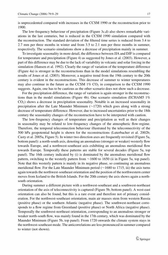
To investigate seasonality in more detail, the difference between JJA and DJF is comparedfor temperature and precipitation (Figure 4) as suggested by Jones et al. (2003). However, apart of this difference may be due to the lack of variability in volcanic and solar forcing in thesimulation (Hansen et al. 1992). Clearly the range of variation of the temperature difference(Figure 4a) is stronger in the reconstructions than in the model simulations resembling theresults of Jones et al. (2003). Moreover, a negative trend from the 19th century to the 20thcentury is evident in the reconstructions. This decrease of summer to winter temperaturesmay also continue in the future as the CCSM 1% CO2 in comparison to the CCSM 1990suggests. Again, one has to be cautious as the other scenario does not show such a decrease.
For the precipitation difference, the range of variation is again stronger in the reconstruc-tions than in the model simulations (Figure 4b). One scenario simulation (ECHAM5 1%CO2) shows a decrease in precipitation seasonality. Notable is an increased seasonality inprecipitation after the Late Maunder Minimum (∼1720) which goes along with a strongdecrease of temperature difference. However, due to increased uncertainties prior to the 18thcentury the seasonality changes of the reconstruction have to be interpreted with caution.
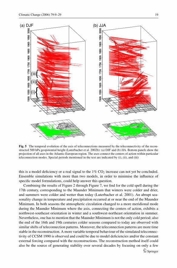
The low-frequency changes of temperature and precipitation as well as their changesin seasonality may be related to low-frequency changes of the atmospheric flow-regime.Therefore, the temporal teleconnection behaviour illustrated by the teleconnectivity of the500 hPa geopotential height is shown for the reconstructions (Luterbacher et al. 2002b;Casty et al. 2005a, Figure 5). In winter two direction axes are frequently revisited (Figure 5a,bottom panel): a north-south axis, denoting an anomalous (stronger or weaker) westerly flowtowards Europe, and a northwest-southeast axis exhibiting an anomalous meridional flowtowards Europe. Temporally these patterns are stable for several decades (Figure 5a, toppanel). The 16th century indicated by (i) is dominated by the anomalous meridional flowpattern, switching to the westerly pattern from ∼1600 to 1650 (ii in Figure 5a, top panel).Note that this westerly pattern is mainly in its negative phase, so continuing an anomalousmeridional flow. For the Late Maunder Minimum period (∼1680 to 1715, iii) the axis turnsagain towards the northwest-southeast orientation and the position of the northwestern centermoves from Iceland to the British Islands. For the 20th century the axis shows again a north-south orientation.
During summer a different picture with a northwest-southeast and a southwest-northeastorientation of the axis of teleconnectivity is captured (Figure 5b, bottom panel). A west-eastorientation can also be found, but this is a rare event and therefore not of primary consid-eration. For the northwest-southeast orientation, main air masses stem from western Russia(positive phase) or the southern Atlantic (negative phase). The southwest-northeast corre-sponds to a flow regime from Greenland (positive phase) or North Africa (negative phase).Temporally the southwest-northeast orientation, corresponding to an anomalous stronger orweaker north-south flow, was mainly found in the 17th century, which was dominated by theMaunder Minimum (Figure 5b, top panel). From 1720 onwards the climate system stays inthe northwest-southeast mode. The anticorrelations are less pronounced in summer comparedto winter (not shown).
Springer
18 Climatic Change (2006) 79:9–29
1500 1600 1700 1800 1900 2000 2100Time [yr]
17
17.5
18
18.5
19
19.5
Tem
pera
ture
[C]
Multi-proxy reconst.ECHAM5 1%CO2CCSM 1%CO2CCSM 1990
1500 1600 1700 1800 1900 2000 2100Time [yr]
-10
-5
0
5
10
15
20
25
Pre
cipi
tatio
n
Multi-proxy reconst.ECHAM5 1%CO2CCSM 1%CO2CCSM 1990
(a)
(b)
2000 500 600
0 300 500 600100 200 400
400300100
Fig. 4 Filtered time series for the difference JJA-DJF (a) European temperature and (b) European precipitation(unit: mm per 3 months). The time series are adjusted to the period 1990–2000 (denoted by the black dot). A31-yr triangular filter is used emphasising the low-frequency variability in the time series. The multi-proxyreconstructions are based on Luterbacher et al. (2004) and Pauling et al. (2006). Note also that the CCSM1990 simulation is for perpetual 1990 conditions, thus the top blue x-axis shows model years
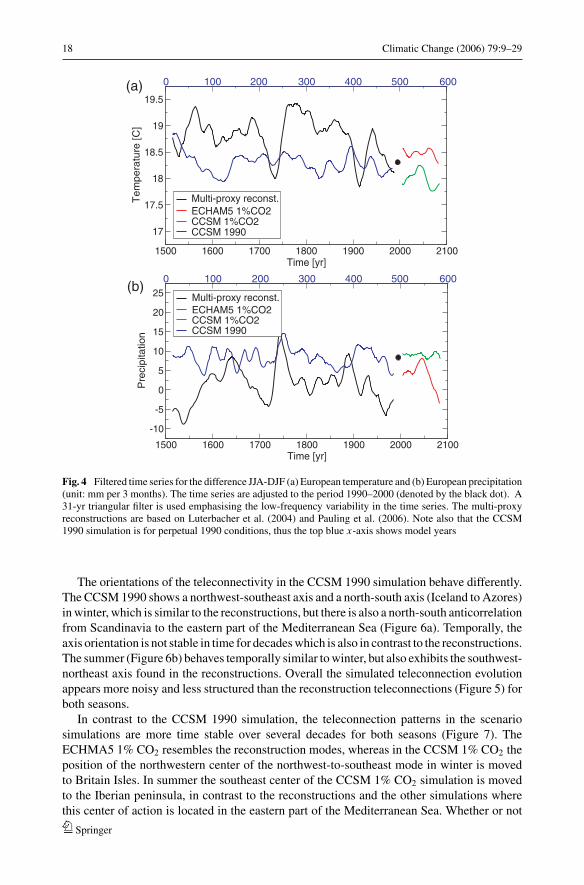
The orientations of the teleconnectivity in the CCSM 1990 simulation behave differently.The CCSM 1990 shows a northwest-southeast axis and a north-south axis (Iceland to Azores)in winter, which is similar to the reconstructions, but there is also a north-south anticorrelationfrom Scandinavia to the eastern part of the Mediterranean Sea (Figure 6a). Temporally, theaxis orientation is not stable in time for decades which is also in contrast to the reconstructions.The summer (Figure 6b) behaves temporally similar to winter, but also exhibits the southwest-northeast axis found in the reconstructions. Overall the simulated teleconnection evolutionappears more noisy and less structured than the reconstruction teleconnections (Figure 5) forboth seasons.
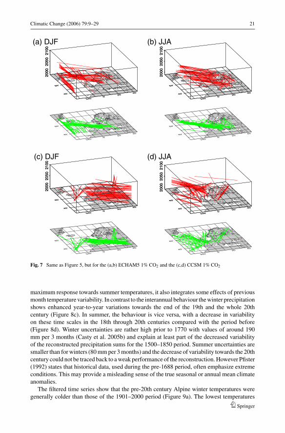
In contrast to the CCSM 1990 simulation, the teleconnection patterns in the scenariosimulations are more time stable over several decades for both seasons (Figure 7). TheECHMA5 1% CO2 resembles the reconstruction modes, whereas in the CCSM 1% CO2 theposition of the northwestern center of the northwest-to-southeast mode in winter is movedto Britain Isles. In summer the southeast center of the CCSM 1% CO2 simulation is movedto the Iberian peninsula, in contrast to the reconstructions and the other simulations wherethis center of action is located in the eastern part of the Mediterranean Sea. Whether or not
Springer
Climatic Change (2006) 79:9–29 19
340˚0˚
20˚40˚
40˚
60˚
340˚0˚
20˚40˚
40˚
60˚
1500
1550
1600
1650
1700
1750
1800
1850
1900
1950
2000
340˚0˚
20˚40˚
40˚
60˚
1500
1550
1600
1650
1700
1750
1800
1850
1900
1950
2000
340˚0˚
20˚40˚
40˚
60˚
340˚0˚
20˚40˚
40˚
60˚
1500
1550
1600
1650
1700
1750
1800
1850
1900
1950
2000
340˚0˚
20˚40˚
40˚
60˚
1500
1550
1600
1650
1700
1750
1800
1850
1900
1950
2000
(a) DJF (b) JJA
(ii)
(iii){{
{(i)
Fig. 5 The temporal evolution of the axis of teleconnections measured by the teleconnectivity of the recon-structed 500 hPa geopotential height (Luterbacher et al. 2002b): (a) DJF and (b) JJA. Bottom panels show theprojection of all axes in the Atlantic-European region. The axes connect the centers of action within particularteleconnection modes. Special periods mentioned in the text are indicated by (i), (ii), and (iii)
this is a model deficiency or a real signal to the 1% CO2 increase can not yet be concluded.Ensemble simulations with more than two models, in order to minimise the influence ofspecific model formulations, could help answer this question.
Combining the results of Figure 2 through Figure 7, we find for the cold spell during the17th century, corresponding to the Maunder Minimum that winters were colder and drier,and summers were colder and wetter than today (Luterbacher et al. 2001). An abrupt sea-sonality change in temperature and precipitation occurred at or near the end of the MaunderMinimum. In both seasons the atmospheric circulation changed to a more meridional modeduring the Maunder Minimum where the axis, connecting the centers of action, exhibits anorthwest-southeast orientation in winter and a southwest-northeast orientation in summer.Nevertheless, one has to mention that the Maunder Minimum is not the only cold period; alsothe end of the 16th and 19th centuries colder seasons compared to today are observed withsimilar shifts of teleconnection patterns. Moreover, the teleconnection patterns are more timestable in the reconstruction. A more variable temporal behaviour of the simulated teleconnec-tivity of CCSM 1990 is observed and could be due to model deficiencies and/or the constantexternal forcing compared with the reconstructions. The reconstruction method itself couldalso be the source of generating stability over several decades by focusing on only a few
Springer
20 Climatic Change (2006) 79:9–29
340˚0˚
20˚40˚
40˚
60˚
340˚0˚
20˚40˚
40˚
60˚
050
100
150
200
250
300
350
400
450
500
340˚0˚
20˚40˚
40˚
60˚
050
100
150
200
250
300
350
400
450
500
340˚0˚
20˚40˚
40˚
60˚
340˚0˚
20˚40˚
40˚
60˚
050
100
150
200
250
300
350
400
450
500
340˚0˚
20˚40˚
40˚
60˚
050
100
150
200
250
300
350
400
450
500
(a) DJF (b) JJA
Fig. 6 Same as Figure 5, but for the 500-year long CCSM simulation with perpetual 1990 conditions
patterns of variability. But, because the reconstructions incorporate external forcing rangingfrom natural (solar and volcanic) to anthropogenic forcing (greenhouse gas emissions) andbecause the scenario simulations show a greater time stability of the teleconnection pattern(compared with the CCSM 1990) we favor an influence of external forcing, thus we hypoth-esise that time-dependent external forcing (solar, volcanic and greenhouse gases) might helpin stabilising the mode temporally.
4 Climate variability in the Alps
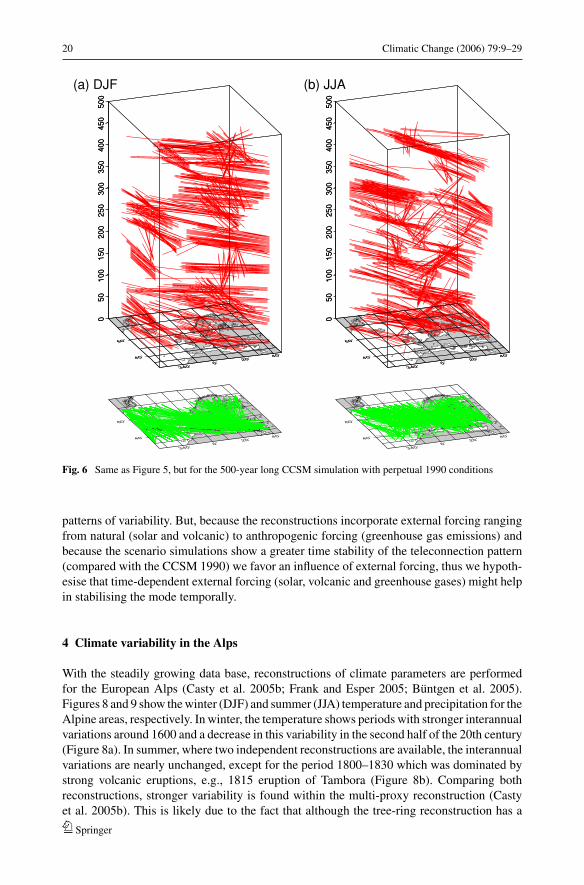
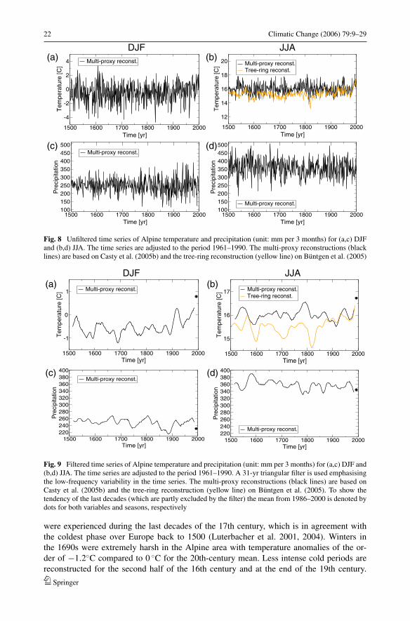
With the steadily growing data base, reconstructions of climate parameters are performedfor the European Alps (Casty et al. 2005b; Frank and Esper 2005; Buntgen et al. 2005).Figures 8 and 9 show the winter (DJF) and summer (JJA) temperature and precipitation for theAlpine areas, respectively. In winter, the temperature shows periods with stronger interannualvariations around 1600 and a decrease in this variability in the second half of the 20th century(Figure 8a). In summer, where two independent reconstructions are available, the interannualvariations are nearly unchanged, except for the period 1800–1830 which was dominated bystrong volcanic eruptions, e.g., 1815 eruption of Tambora (Figure 8b). Comparing bothreconstructions, stronger variability is found within the multi-proxy reconstruction (Castyet al. 2005b). This is likely due to the fact that although the tree-ring reconstruction has a
Springer
Climatic Change (2006) 79:9–29 21
340˚0˚
20˚40˚
40˚
60˚
340˚0˚
20˚40˚
40˚
60˚
2000
2050
2100
340˚0˚
20˚40˚
40˚
60˚
2000
2050
2100
340˚0˚
20˚40˚
40˚
60˚
340˚0˚
20˚40˚
40˚
60˚
2000
2050
2100
340˚0˚
20˚40˚
40˚
60˚
2000
2050
2100
340˚0˚
20˚40˚
40˚
60˚
340˚0˚
20˚40˚
40˚
60˚
2000
2050
2100
340˚0˚
20˚40˚
40˚
60˚
2000
2050
2100
340˚0˚
20˚40˚
40˚
60˚
340˚0˚
20˚40˚
40˚
60˚
2000
2050
2100
340˚0˚
20˚40˚
40˚
60˚
2000
2050
2100
(a) DJF (b) JJA
(d) JJA(c) DJF
Fig. 7 Same as Figure 5, but for the (a,b) ECHAM5 1% CO2 and the (c,d) CCSM 1% CO2
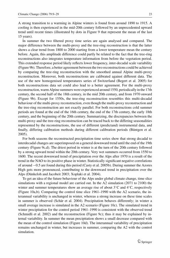
maximum response towards summer temperatures, it also integrates some effects of previousmonth temperature variability. In contrast to the interannual behaviour the winter precipitationshows enhanced year-to-year variations towards the end of the 19th and the whole 20thcentury (Figure 8c). In summer, the behaviour is vice versa, with a decrease in variabilityon these time scales in the 18th through 20th centuries compared with the period before(Figure 8d). Winter uncertainties are rather high prior to 1770 with values of around 190mm per 3 months (Casty et al. 2005b) and explain at least part of the decreased variabilityof the reconstructed precipitation sums for the 1500–1850 period. Summer uncertainties aresmaller than for winters (80 mm per 3 months) and the decrease of variability towards the 20thcentury could not be traced back to a weak performance of the reconstruction. However Pfister(1992) states that historical data, used during the pre-1688 period, often emphasize extremeconditions. This may provide a misleading sense of the true seasonal or annual mean climateanomalies.
The filtered time series show that the pre-20th century Alpine winter temperatures weregenerally colder than those of the 1901–2000 period (Figure 9a). The lowest temperatures
Springer
22 Climatic Change (2006) 79:9–29
1500 1600 1700 1800 1900 2000Time [yr]
-4
-2
0
2
4T
empe
ratu
re [C
]Multi-proxy reconst.
1500 1600 1700 1800 1900 2000Time [yr]
100150200250300350400450500
Pre
cipi
tatio
n
Multi-proxy reconst.
1500 1600 1700 1800 1900 2000Time [yr]
12
14
16
18
20
Tem
pera
ture
[C] Multi-proxy reconst.
Tree-ring reconst.
1500 1600 1700 1800 1900 2000Time [yr]
100150200250300350400450500
Pre
cipi
tatio
n
Multi-proxy reconst.
(c)
(a) (b)
(d)
JJADJF
Fig. 8 Unfiltered time series of Alpine temperature and precipitation (unit: mm per 3 months) for (a,c) DJFand (b,d) JJA. The time series are adjusted to the period 1961–1990. The multi-proxy reconstructions (blacklines) are based on Casty et al. (2005b) and the tree-ring reconstruction (yellow line) on Buntgen et al. (2005)
1500 1600 1700 1800 1900 2000Time [yr]
-1
0
1
Tem
pera
ture
[C] Multi-proxy reconst.
1500 1600 1700 1800 1900 2000Time [yr]
220240260280300320340360380400
Pre
cipi
tatio
n
Multi-proxy reconst.
1500 1600 1700 1800 1900 2000Time [yr]
15
16
17
Tem
pera
ture
[C] Multi-proxy reconst.
Tree-ring reconst.
1500 1600 1700 1800 1900 2000Time [yr]
220240260280300320340360380400
Pre
cipi
tatio
n
Multi-proxy reconst.
(b)
(d)(c)
(a)DJF JJA
Fig. 9 Filtered time series of Alpine temperature and precipitation (unit: mm per 3 months) for (a,c) DJF and(b,d) JJA. The time series are adjusted to the period 1961–1990. A 31-yr triangular filter is used emphasisingthe low-frequency variability in the time series. The multi-proxy reconstructions (black lines) are based onCasty et al. (2005b) and the tree-ring reconstruction (yellow line) on Buntgen et al. (2005). To show thetendency of the last decades (which are partly excluded by the filter) the mean from 1986–2000 is denoted bydots for both variables and seasons, respectively
were experienced during the last decades of the 17th century, which is in agreement withthe coldest phase over Europe back to 1500 (Luterbacher et al. 2001, 2004). Winters inthe 1690s were extremely harsh in the Alpine area with temperature anomalies of the or-der of −1.2◦C compared to 0 ◦C for the 20th-century mean. Less intense cold periods arereconstructed for the second half of the 16th century and at the end of the 19th century.
Springer
Climatic Change (2006) 79:9–29 23
A strong transition to a warming in Alpine winters is found from around 1890 to 1915. Acooling is then experienced in the mid-20th century followed by an unprecedented upwardtrend until recent times (illustrated by dots in Figure 9 that represent the mean of the last15 years).
In summer the two filtered proxy time series are again analysed and compared. Themajor difference between the multi-proxy and the tree-ring reconstruction is that the lattershows a clear trend from 1800 to 2000 starting from a lower temperature mean the centurybefore. Again, this amplitude difference could partly be related to the fact that the tree-ringreconstructions also integrates temperature information from before the vegetation period.This extended response period likely reflects lower frequency, inter-decadal scale variability(Figure 9b). Therefore, a better agreement between the two reconstructions could be achievedby comparing the tree-ring reconstruction with the smoothed annual Alpine multi-proxyreconstruction. Moreover, both reconstructions are calibrated against different data. Theuse of the new homogenised temperatures series of Switzerland (Begert et al. 2005) forboth reconstructions data set could also lead to a better agreement. For the multi-proxyreconstruction, warm Alpine summers were experienced around 1550, periodically in the 17thcentury, the second half of the 18th century, in the mid 20th century, and from 1970 onward(Figure 9b). Except for 1550s, the tree-ring reconstruction resembles this multi-decadalbehaviour of the multi-proxy reconstruction, even though the multi-proxy reconstruction andthe tree-ring reconstruction are not exactly parallel. For both reconstructions cold summerperiods are found at the end of the 16th century, the end of the 17th century, the early 18thcentury, and the beginning of the 20th century. Summarizing, the discrepancies between themulti-proxy and the tree-ring reconstruction can be traced back to the differing seasonalitiesrepresented by the reconstructions, the use of different (predictand) instrumental data, andfinally, differing calibration methods during different calibration periods (Buntgen et al.2005).
For both seasons the reconstructed precipitation time series show that strong decadal tointerdecadal changes are superimposed on a general downward trend until the end of the 19thcentury (Figure 9c,d). The driest period in winter is at the turn of the 20th century followedby a strong upward trend within the 20th century. Very wet summers occurred from 1550 to1600. The recent downward trend of precipitation over the Alps after 1970 is a result of thetrend in the NAO to its positive phase in winter. Statistically significant negative correlationsof around −0.5 are found during this period (Casty et al. 2005b). During summer the AzoresHigh gets more pronounced, contributing to the downward trend in precipitation over theAlps (Dunkeloh and Jacobeit 2003; Xoplaki et al. 2004).
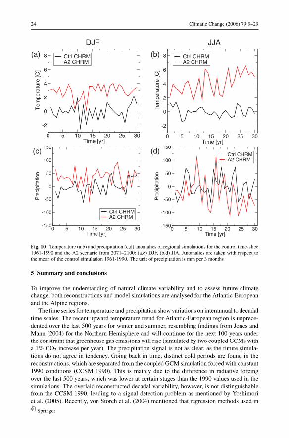
To get an idea of the future behaviour of the Alps under global climate change, time slicesimulations with a regional model are carried out. In the A2 simulation (2071 to 2100) thewinter and summer temperatures show an average rise of about 3◦C and 4◦C, respectively(Figure 10a,b). Comparing the control time slice 1961–1990 with the A2 scenario, the in-terannual variability is unchanged in winter, whereas a strong increase on these time scalesin summer is observed (Schar et al. 2004). Precipitation behaves differently; in winter asmall average increase is simulated in the A2 scenario (Figure 10c). The simulated trend inwinter precipitation for the control period 1961–1990 is consistent with the observed trend(Schmidli et al. 2002) and the reconstruction (Figure 9c); thus it may be explained by in-ternal variability. In summer the mean precipitation shows a small decrease compared withthe mean of the control simulation (Figure 10d). The interannual variability of precipitationremains unchanged in winter, but increases in summer, comparing the A2 with the controlsimulation.
Springer
24 Climatic Change (2006) 79:9–29
0 5 10 15 20 25 30Time [yr]
-2
0
2
4
6
8
Tem
pera
ture
[C]
Ctrl CHRMA2 CHRM
0 5 10 15 20 25 30Time [yr]
-150
-100
-50
0
50
100
150
Pre
cipi
tatio
n
Ctrl CHRMA2 CHRM
0 5 10 15 20 25 30Time [yr]
-150
-100
-50
0
50
100
150
Pre
cipi
tatio
nCtrl CHRMA2 CHRM
0 5 10 15 20 25 30Time [yr]
-2
0
2
4
6
8
Tem
pera
ture
[C]
Ctrl CHRMA2 CHRM
(a) (b)
(d)(c)
DJF JJA
Fig. 10 Temperature (a,b) and precipitation (c,d) anomalies of regional simulations for the control time-slice1961-1990 and the A2 scenario from 2071–2100: (a,c) DJF, (b,d) JJA. Anomalies are taken with respect tothe mean of the control simulation 1961-1990. The unit of precipitation is mm per 3 months
5 Summary and conclusions
To improve the understanding of natural climate variability and to assess future climatechange, both reconstructions and model simulations are analysed for the Atlantic-Europeanand the Alpine regions.
The time series for temperature and precipitation show variations on interannual to decadaltime scales. The recent upward temperature trend for Atlantic-European region is unprece-dented over the last 500 years for winter and summer, resembling findings from Jones andMann (2004) for the Northern Hemisphere and will continue for the next 100 years underthe constraint that greenhouse gas emissions will rise (simulated by two coupled GCMs witha 1% CO2 increase per year). The precipitation signal is not as clear, as the future simula-tions do not agree in tendency. Going back in time, distinct cold periods are found in thereconstructions, which are separated from the coupled GCM simulation forced with constant1990 conditions (CCSM 1990). This is mainly due to the difference in radiative forcingover the last 500 years, which was lower at certain stages than the 1990 values used in thesimulations. The overlaid reconstructed decadal variability, however, is not distinguishablefrom the CCSM 1990, leading to a signal detection problem as mentioned by Yoshimoriet al. (2005). Recently, von Storch et al. (2004) mentioned that regression methods used in
Springer
Climatic Change (2006) 79:9–29 25
Northern Hemisphere reconstructions of this kind underestimate low-frequency variability,which leads to the conclusion that the real climate variability shows stronger decadal fluc-tuations and therefore it might be distinguishable from CCSM 1990. However, recent work(Mann et al. 2005; Goosse et al. 2005) suggests that the results of von Storch et al. (2004)may be overstated, implying that the decadal fluctuations reconstructed may be relativelyaccurate. In this case the signal detection problem would remain. The changes in seasonalityshow that the reconstructions have a broader range than the model simulations, resemblingthe results of Jones et al. (2003). A clear signal in the future could not be detected; as the twosimulations again do not agree.
Illustrated by the teleconnectivity we showed that low-frequency changes of large-scaleatmospheric circulation flow control at least part of the temperature and precipitation variabil-ity, e.g., the meridional circulation in the late Maunder Minimum connected with an anoma-lously cold period and more zonal flow regime with warm temperatures in the 20th century.Temporally, differences between the reconstructed and the simulated teleconnectivity usingCCSM 1990 are likely to be due to the constant external forcing of CCSM 1990. Becausethe scenario simulations show temporally stable axes of teleconnection patterns over severaldecades, similar to the reconstructions, we hypothesise that time-dependent external forcing(solar, volcanic and greenhouse gases) might support a temporal stabilisation of the patterns.Future investigations of an ensemble of transient model simulations from 1500 onwardswill help to address this question in more detail. It will also give us the possibility to test thereconstruction method in order to exclude exclude those, which are the source of stabilization.
Analysing the low-frequency behaviour of temperature and precipitation, the Alpine areashows stronger amplitudes than the Atlantic-European region in summer and winter. How-ever, this result likely derives from the smaller area considered and does not necessarily implythat mountainous regions are more sensitive to large-scale variability and climate change.Projections for the future climate with a regional model show, beside a clear temperatureincrease in both seasons, a change in interannual variability in summer. Temperature andprecipitation show broader distributions, which could be partly explained by a soil moistureprecipitation feedback mechanism (Schar et al. 1999, 2004). However, the reconstructionsshow an opposite behaviour, comparing the period after 1900 (which is already influenced byincreasing greenhouse gas emissions) with the centuries before. Still, it can not be decidedwhether or not this is due to the underestimation of variability of regression techniques usedfor the reconstructions, or the regional model’s overestimation of the variability, or the pastwarming was small compared with the expected future warming. A further improvement of thereconstruction methods as well as multi-model ensemble approaches (using different regionalmodels nested in different global models) could give a more comprehensive picture in future.
Acknowledgements This work is supported by the National Centre for Competence in Research (NCCR) inClimate funded by the Swiss National Science Foundation. Some data used in the study has been providedby the Climatic Research Unit (CRU). Part of the simulations are performed at the Swiss Center of ScientificComputing (SCSC) in Manno, Switzerland. We would like thank E. R. Wahl, J. F. Gonzalez-Rouco, and theanonymous referee for very helpful suggestions.
References
Appenzeller C, Stocker TF, Anklin M (1998) North Atlantic Oscillation dynamics recorded in Greenland icecores. Science 282:446–449
Arakawa A, Lamb VR (1981) A potential enstrophy and energy conserving scheme for the shallow waterequations. Mon Wea Rev 109:18–36
Springer
26 Climatic Change (2006) 79:9–29
Bauer E, Claussen M, Brovkin V, Huenerbein A (2003) Assessing climate forcings of the Earth system forthe past millennium. Geophys Res Lett 30, DOI:10.1029/2002GL016639
Begert M, Schlegel T, Kirchhofer W (2005) Homoteneous temperature and precipitation series of Switzerlandfrom 1864 to 2000. Int J Climatol 25:65–80
Blackmon ML, Boville B, Bryan F, Dickinson R, Gent Kiehl J, Moritz R, Randall D, Shukla J, Solomon S,Bonan G, Doney S, Fung I, Hack J, Hunke E, Hurrell J, Kutzbach J, Meehl J, Otto-Bliesner B, SaravananR, Schneider EK, Sloan L, Spall M, Taylor K, Tribbia J, Washington W (2001) The community climatesystem model. Bull Am Meteorol Soc 82:2357–2388
Bohm R, Auer I, Brunetti M, Maugeri M, Nanni T, Schoner W (2001) Regional temperature variability in theEuropean Alps: 1760–1998 from homogenized instrumental series. Int J Climatol 21:1779–1801
Bradley R, Jones PD (1993) Little Ice Age” summer temperature variations: Their nature and relevance torecent global warming trends. The Holocene 3:367–376
Briffa KR, Jones PD, Bartholin TS, Eckstein D, Schweingruber FH, Karlen W, Zetterberg P, Eronen M (1992)Fennoscandian summers from AD 500: Temperature changes on short and long timescales. Clim Dyn7:111–119
Briffa KR, Osborn TJ, Schweingruber FH, Harris IC, Jones PD, Shiyatov SG, Vaganov EA (2001) Low-frequency temperature variations from a northern tree-ring density network. J Geophys Res 106:2929–2941
Buntgen U, Esper J, Frank DC, Nicolussi K, Schmidhalter M (2005) A 1052-year tree-ring proxy for Alpinesummer temperatures. Clim Dyn 25:141–153
Casty C, Handorf D, Raible CC, Luterbacher J, Weisheimer A, Xoplaki E, Gonzalez-Rouco JF, DethloffK, Wanner H (2005a) Recurrent climate winter regimes in reconstructed and modelled 500 hPageopotential height fields over the North Atlantic-European sector 1659–1990. Clim Dyn 24:809–822,DOI:10.1007/s00382-004-0496-8
Casty C, Wanner H, Luterbacher J, Esper J, Bohm R (2005b) Temperature und precipitation variability in theEuropean Alps since 1500. Int J Climatol 25:1855–1880
Cheng W, Beck R, Rooth C (2004) Multi-decadal thermohaline variability in an ocean-atmosphere generalcirculation model. Clim Dyn 22:573–590, DOI:10.1007/s00382-004-400-6
Cook ER, D’Arrigo RD, Mann ME (2002) A well-verified, multiproxy reconstruction of the winter NorthAtlantic Oscillation index since AD 1400. J Climate 15:1754–1764
Cook ER, Esper J, D’Arrigo RD (2004) Extra-tropical Northern Hemisphere land temperature variability overthe past 1000 years. Quat Sci Rev 23:2063–2074
Crowley TJ (2000) Causes of climate change over the past 1000 years. Science 289:270–277Dunkeloh A, Jacobeit J (2003) Circulation dynamics of Mediterranean precipitation variability 1948–98. Int
J Climatol 23:1843–1866Esper J (2000) Long term tree-ring variations in Junipers at the upper timberline in the Karakorum (Pakistan).
The Holocene 10:253–260Esper J, Cook ER, Schweingruber FH (2002a) Low-frequency signals in long tree-line chronologies for
reconstructing past temperature variability. Science 295:2250–2253Esper J, Frank DC, Wilson RJS (2004) Climate reconstructions: Low-frequency ambition and high-frequency
ratification. EOS, Trans Am Geophys Union 85:113,120Esper J, Schweingruber FH, Winiger M (2002b) 1300 years of climate history for Western Central Asia
inferred from tree-rings. The Holocene 12:267–277Esper J, Shiyatov SG, Mazepa VS, Wilson RJS, Graybill DA, Funkhouser G (2003) Temperature-sensitive
Tien Shan tree ring chronologies show multi-centennial growth trends. Clim Dyn 21:699–706Frank DC, Esper J (2005) Temperature reconstructions and comparison with instrumental data from a tree-ring
network for the European Alps. Int J Climatol 25:1437–1454Frei C, Christensen JH, Deque M, Jacob D, Jones RG, Vidale PL (2003) Daily precipitation statistics in
regional climate models: Evaluation and intercomparison for the European Alps. J Geophys Res 108(D3),4124, DOI: 10.1029/2002JD002287
Gibson JK, Kallberg P, Uppala S, Hernandez A, Nomura A, Serrano A (1999) ERA description, Version 2Technical report, ERA-15 Project Report Series, No. 1, ECMWF, Reading, UK. p. 74
Goosse H, Crwoley TJ, Zorita E, Ammann H, Renssen CM, Driesschaert E (2005) Modelling the climate ofthe last millennium: What causes the differences between simulations. Geophys Res Lett 32, L06710,DOI:10.1029/2005GL022368
Grotzner A, Latif M, Barnett TP (1998) A decadal cycle in the North Atlantic ocean as simulated by the ECHOcoupled GCM. J Climate 11:831–847
Guiot J, Nicault A, Rathgeber C, Edouard J, Guibal F, Pichard G, Till C (2005) Last-millennium summer-temperature variations in western Europe based on proxy data. Holocene 15:489–500
Springer
Climatic Change (2006) 79:9–29 27
Hagemann S, Duemenil-Gates, L (2001) Validation of the hydrological cycle of ECMWF and NCEP reanalysesusing the MPI hydrological discharge model. J Geophys Res 106:1503–1510
Hansen J, Lacis A, Ruedy R, Sato M (1992) Potential climate impact of Mount Pinatubo eruption. GeophysRes Lett 19:215–218
Hurrell, JW (1995) Decadal trends in the North Atlantic Oscillation: Regional temperatures and precipitation.Science 269:676–679
Hurrell JW, Kushnir Y, Ottersen G, Visbeck M (2003) The North Atlanitc Oscillation: Climate Significanceand Environmental Impact, Vol. 134. Geophysical Monograph Series. p. 279
Hurrell JW, Loon HV (1997) Decadal variations in climate associated with the North Atlantic Oscillation.Clim Change 36:301–326
IPCC (2001) Climate Change 2001: The Scientific Basis. Cambridge, UK and New York, NY, USA: CambridgeUniversity Press. Contribution of Working Group I to the Third Assessment Report of the IntergovenmentalPanel on Climate Change, p. 881
Jacobeit J, Wanner H, Luterbacher J, Beck C, Philipp A, Sturm K (2003) Atmospheric circulation variabilityin the North-Atlantic-European area since the mid-seventeenth century. Clim Dyn 20:341–352
Jones PD, Briffa KR, Barnett TP, Tett SFB (1998) High-resolution palaeoclimatic records for the lastmillennium: Interpretation, integration and comparison with General Circulation Model control-runtemperatures. The Holocene 8:455–471
Jones PD, Briffa KR, Osborn TJ (2003) Changes in the Northern Hemisphere annual cycle: Implications forpaleoclimatology. J Geophys Res 108, DOI:10.1029/2003JD003695
Jones PD, Mann ME (2004) Climate over past millennia. Rev Geophys 42, RG2002,DOI:10.1029/2003RG000143
Jones RG, Murphy JM, Hassell DC, Taylor R (2001) Ensemble mean changes in a simulation of the Europeanclimate of 2071–2100 using the new Hadley Centre Regional modelling system HadAM3H/HadRM3H,Technical report, Hadley Centre, Exeter, UK, available at http://prudence.dmi.dkl
Kalnay E, Kanamitsu M, Kistler R, Collins W, Coauthors (1996) The NCEP/NCAR 40 year reanalysisproject. Bull Am Meteor Soc 77:437–471
Kiehl JT, Hack JJ, Bonan GB, Boville BA, Williamson DL, Rasch PJ (1998) The National Center forAtmospheric Research Community Climate Model: CCM3. J Clim 11:1131–1149
Kistler R, Kalnay E, Collins W, Saha S, Coauthors (2001) The NCEP-NCAR 50-year reanalysis: Monthlymeans CD-ROM and documentation. Bull Am Meteor Soc 77:437–471
Latif M, Roeckner E, Botzet M, Esch M, Haak H, Hagemann S, Jungclaus J, Legutke S, Marsland S,Mikolajewicz U (2004) Reconstructing, monitoring, and predicting multidecadal-scale changes in theNorth Atlantic Thermohaline Circulation with sea surface temperature. J Clim 17:1606–1614
Luterbacher J, Dietrich D, Xoplaki E, Grosjean M, Wanner H (2004) European seasonal and annualtemperature variability, trends, and extremes since 1500. Science 303:1499–1503
Luterbacher J, Rickli R, Xoplaki E, Tinguely C, Beck C, Pfister C, Wanner H (2001) The late MaunderMinimum (1675–1715) – a key period for studying decadal scale climatic change in Europe. ClimChange 49:441–462
Luterbacher J, Schmutz C, Gyalistras D, Xoplaki E, Wanner H (1999) Reconstruction of monthly NAO andEU indices back to AD 1675. Geophys Res Lett 26:2745–2748
Luterbacher J, Xoplaki E, Dietrich D, Jones PD, Davies TD, Portis D, Gonzalez-Rouco JF, von Storch H,Gyalistras D, Casty C, Wanner H (2002a) Extending North Atlantic Oscillation reconstructions back to1500. Atmos Sci Lett 2:114–124
Luterbacher J, Xoplaki E, Dietrich D, Rickli R, Jacobeit J, Beck C, Gyalistras D, Schmutz C, Wanner H(2002b) Reconstruction of sea level pressure fields over the Eastern North Atlantic and Europe back to1500. Clim Dyn 18:545–561
Mann ME, Bradley RS, Hughes MK (1998) Global-scale temperature patterns and climate forcing over thepast six centuries. Nature 392:779–787
Mann ME, Rutherford S, Wahl ER, Ammann CM (2005) Testing the fidelity of methodologies used inproxy-based reconstructions of past climate. J Clim 18:4097–4107
Marshall J, Johnson H, Goodman J (2001) A study of the interaction of the North Atlantic Oscillation withocean circulation. J Clim 14:1399–1421
Marsland SJ, Haak H, Jungclaus JH, Latif M, Roeske F (2003) The Max-Planck-Institute global ocean/seaice model with orthogonal curvilinear coordinates. Ocean Model 5:91–127
Meehl GA, Washington WM, Wigley TML, Arblaster JM, Dai A (2003) Solar and greenhouse gas forcingand climate response in the twentieth century. J Clim 16:426–444
Mitchell TD, Carter TR, Jones PD, Hulme M, New, M (2004) A comprehensive set of high-resolutiongrids of monthly climate for Europe and the globe: The observed record (1901–2000) and 16 scenarios(2001–2100). Technical Report Working Paper 55, Tyndall Center for Climate Change Research
Springer
28 Climatic Change (2006) 79:9–29
Moberg A, Sonechkin DM, Holmgren K, Datsenko NW, Karlen W (2005) Highly variable NorthernHemisphere temperatures reconstructed from low- and high-resolution proxy data. Nature 433:613–617
New M, Hulme M, Jones PD (2000) Representing twentieth-century space-time climate variability. Part II:Development of 1901–1996 monthly grids of terrestrial surface climate. J Clim 13:2217–2238
Overpeck J, Hughen K, Hardy D, Bradley R, Case R, Douglas M, Finney, B, Gajewski K, Jacoby G, JenningsA, Lamoureux S, Lasca A, MacDonald G, Moore J, Retelle M, Smith S, Wolfe A, Zielinski G (1997)Arctic environmental change of the last four centuries. Science 278:1251–1256
Pauling A, Luterbacher J, Casty C, Wanner H (2006) 500 years of gridded high-resolution precipitationreconstructions over Europe and the connection to large-scale circulation. Clim Dyn 26:387–405
Pfister C (1992) Monthly temperature and precipitation in Central Europe 1525–1979: Quantifying docu-mentary evidence on weather and its effects. In: Bradley RS, Jones PD (eds) Climate since A.D. 1500.Routledge, London
Pope DV, Gallani M, Rowntree R, Stratton A (2000) The Impact of new physical parameterizations in theHadley Centre climate model HadAM3. Clim Dyn 16:123–146
Raible CC, Luksch U, Fraedrich K (2004) Precipitation and Northern Hemisphere Regimes. Atmos Sci Lett5:43–55, DOI:10.1016/j.atmoscilet.2003.12.001
Raible CC, Luksch U, Fraedrich K, Voss R (2001) North Atlantic decadal regimes in a coupled GCMsimulation. Clim Dyn 18:321–330
Raible CC, Stocker TF, Yoshimori M, Renold M, Beyerle U, Casty C, Luterbacher J (2005) Northern Hemi-spheric trends of pressure indices and atmospheric circulation patterns in observations, reconstructions,and coupled GCM simulations. J Clim 18:3968–3982
Renold M, Beyerle U, Raible CC, Knutti R, Stocker TF, Craig T (2004) Climate modeling with a Linuxcluster, EOS, Trans Am Geophys Union 85:292
Rind D, Lean J, Healy R (1999) Simulated time-dependent climate response to solar radiative forcing since1600. J Geophys Res 104:1973–1990
Roeckner E, Bauml G, Bonaventura L, Brokopf R, Esch M, Giorgetta M, Hagemann S, Kirchner I, KornbluehL, Manzini E, Rhodin A, Schlese U, Schulzweida U, Tompkins A (2003) The atmospheric generalcirculation model ECHAM5: Part I: Model description, Technical Report 349, Max-Planck-Institut,Hamburg, Germany
Schar C, Luthi D, Beyerle U, Heise E (1999) The soil-precipitation feedback: A process study with a regionalclimate model. J Clim 12:722–741
Schar C, Vidale PL, Luthi, D, Haberli C, Liniger MA, Appenzeller C (2004) The role of increasing temperaturevariability in European summer heatwaves. Nature 427:332–336
Schmidli J, Schmutz C, Frei C, Wanner H, Schar C (2002) Mesoscale precipitation variability in the Alpineregion during the 20th century. Int J Climatol 22:1049–1074
Shindell DT, Schmidt GA, Miller RL, Mann ME (2003) Volcanic and solar forcing of climate change duringthe preindustrial era. J Clim 16:4094–4107
Shindell DT, Schmidt GA, Miller RL, Rind D (2001) Northern Hemisphere winter climate response togreenhouse gas, ozone, solar, and volcanic forcing. J Geophy Res 106:7193–7210
Terray L, Valcke S, Piacentini A (1998) The OASIS coupler user guide, version 2.2, Technical ReportTR/CMGC/98–05, CERFACS
Ulbrich U, Christoph M (1999) A shift of the NAO and increasing storm track activity over Europe due toanthropogenic Greenhouse gas forcing, Clim Dyn 15:551–559
Vidale PL, Luthi D, Frei C, Seneviratne SI, Schar C (2003) Predictability and uncertainty in a regional climatemodel. J Geophys Res 108, DOI:10.1029/2002JD002810
Vinther BM, Johnsen SJ, Andersen KK, Clausen HB, Hansen AW (2003) NAO signal recorded in the stableisotopes of Greenland ice cores. Geophys Res Lett 30(7), 1387, DOI: 10.1029/2002GL016193
von Storch H, Zorita E, Jones J, Dimitriev Y, Gonzalez-Rouco F, Tett S (2004) Reconstructing past climatefrom noisy data. Science 306:679–682, DOI:10.1126/science.1096109
Wallace JM, Gutzler DS (1981) Teleconnections in the geopotential height field during the NorthernHemisphere winter. Mon Wea Rev 109:782–812
Wanner H, Bronnimann S, Casty C, Gyalistras D, Luterbacher J, Schmutz C, Stephenson DB, Xoplaki E(2001) North Atlantic Oscillation—concepts and studies. Survey Geophys 22:321–382
Wild M, Calanca P, Scherrer SC, Ohmura A (2003) Effects of polar ice sheets on global sea level inhigh-resolution greenhouse scenarios, J Geophys Res 108, DOI:10.1029/2002JD002451
Wolff JO, Maier-Reimer E, Legutke S (1997) The Hamburg Ocean primitive equation model HOPE. TechnicalReport 13, Deutsches Klimarechenzentrum, Hamburg, Germany
Xoplaki E, Gonzalez-Rouco JF, Luterbacher J, Wanner H (2004) Wet season Mediterranean precipitationvariability: Influence of large-scale dynamics and trends. Clim Dyn 23:63–78
Springer

Climatic Change (2006) 79:9–29 29
Xoplaki E, Luterbacher J, Paeth H, Dietrich D, Steiner N, Grosjean M, Wanner H (2005) European springand autumn temperature variability and change of extremes over the last half millennium. Geophys ResLett 32, L15713, DOI: 10.1029/2005GL023424
Yoshimori M, Stocker TF, Raible CC, Renold M (2005) Internal and externally-forced varibilities in anensemble of climate simulations of the Maunder Minimum. J Clim 18:4253–4270
Springer
Climatic Change (2006) 79:31–63DOI 10.1007/s10584-006-9076-8
Challenges posed by and approaches to the studyof seasonal-to-decadal climate variability
Cornelia Schwierz · Christof Appenzeller ·Huw C. Davies · Mark A. Liniger · Wolfgang Muller ·Thomas F. Stocker · Masakazu Yoshimori
Received: 9 December 2004 / Accepted: 14 December 2005 / Published online: 4 November 2006C© Springer Science + Business Media B.V. 2006
Abstract The tasks of providing multi-decadal climate projections and seasonal plus sub-seasonal climate predictions are of significant societal interest and pose major scientificchallenges. An outline is presented of the challenges posed by, and the approaches adoptedto, tracing the possible evolution of the climate system on these various time-scales. Firstan overview is provided of the nature of the climate system’s natural internal variationsand the uncertainty arising from the complexity and non-linearity of the system. Thereafterconsideration is given sequentially to the range of extant approaches adopted to study andderive multi-decadal climate projections, seasonal predictions, and significant sub-seasonalweather phenomena. For each of these three time-scales novel results are presented thatindicate the nature (and limitations) of the models used to forecast the evolution, and illustratethe techniques adopted to reduce or cope with the forecast uncertainty. In particular, thecontributions (i) appear to exemplify that in simple climate models uncertainties in radiativeforcing outweigh uncertainties associated with ocean models, (ii) examine forecast skillsfor a state-of-the-art seasonal prediction system, and (iii) suggest that long-lived weatherphenomena can help shape intra-seasonal climate variability. Finally, it is argued, that co-consideration of all these scales can enhance our understanding of the challenges associatedwith uncertainties in climate prediction.
C. Schwierz (�) · H. C. DaviesInstitute for Atmospheric and Climate Science, ETH Zurich, Switzerlande-mail: [email protected]
C. Appenzeller · M. A. Liniger · W. MullerFederal Office of Meteorology and Climatology (MeteoSwiss), Switzerland
W. MullerPresent Address: MPI for Meteorology, Hamburg, Germany
T. F. Stocker · M. YoshimoriClimate and Environmental Physics, Physics Institute, University of Bern, Switzerland
M. YoshimoriPresent Address: Center for Environmental Prediction, Rutgers University, USA
Springer
32 Climatic Change (2006) 79:31–63
1 Introduction
In the context of possible anthropogenically-induced climate change considerable effort isbeing devoted to providing projections of the evolution of the climate system over the 21stcentury (e.g., IPCC 2001). These projections should in principle not only yield an indicationof the development of a climate mean but also supply the associated behaviour of and changeof that variability (e.g., Mearns et al. 1984; Schneider 2000). Indeed it is possible thatclimate change could be manifested at least in part by changes in the nature and amplitudeof the variability. Thus it is important to improve both our understanding and our predictivecapability of climate variability.
Here the focus is on the atmospheric component of the climate system and on multi-decadal, seasonal, and sub-seasonal time-scales. In this time-range key processes influencingthe variation and change range from the direct and indirect effects of increased greenhouse gasemissions, the longer-term memory of the oceans, atmosphere-ocean and atmosphere-landsurface interactions, and the internal dynamics of the atmosphere itself.
In the following sections, an overview is provided of the challenges associated withdeveloping projections on these different time-scales. In Section 2 summaries are givenof the concepts of climate variability; the prediction-model hierarchy; forecast uncertaintyand the probabilistic approach to quantify forecast uncertainty. The subsequent sectionsare devoted to consideration of the methods and challenges pertaining to each time-scale,and providing novel results that exemplify the complexity and temporal interrelations andspecific intricacies. The individual sections comprise a discussion of the utility of a hierarchyof climate models to reduce the uncertainty of climate projections on the multi-decadaltime scales (Section 3); the ingredients of current schemes for seasonal prediction and thequantitative assessment of forecast skill (Section 4); and a discussion of the dynamics ofsignificant sub-seasonal weather phenomena and their linkage to climate variation (Section 5).Finally some comments are proffered on the synergies that exist between the proceduresemployed on these different time-scales and possible avenues for future research (Section 6).
2 Basic concepts
2.1 Climate variability, impacts and trends
Climate varies naturally on a vast range of time-scales under the influence of both externalforcing or internal variability of the system. Internal variability occurs, because in a system ofcomponents with non-linear interactions and very different response times the componentstend to vary constantly and not achieve a state of inter-component equilibrium. The responseof the climate to external forcings and to the internal variability is further complicated byfeedbacks and non-linear responses of the components (IPCC 2001). On the regional scale,climate variability often manifests itself in geographically anchored spatial patterns withchanging amplitude (and sign). These patterns determine the local climatic conditions andhence it is also highly desirable to understand and predict them accurately.
The strongest large-scale climate variation on seasonal to inter-annual time-scales has itsorigin in the tropical-subtropical Pacific and is known as the El Nino/Southern Oscillation(ENSO, see reviews of Philander 1990; Trenberth et al. 1998), that typically occurs every 2–7years. The ENSO phenomenon consists of a coupled interplay between the atmosphere andocean. It is associated with a see-saw in atmospheric pressure between the eastern and westernPacific and the occurrence of warm ocean-temperature anomalies in the upper few hundred
Springer
Climatic Change (2006) 79:31–63 33
meters of the eastern and central tropical Pacific. Marked shifts in weather conditions, inparticular precipitation patterns, are associated with ENSO and are not only located in thecentral Pacific, but also over adjacent continents (Trenberth and Hurrell 1994) and in moreremoved regions around the globe (Diaz and Markgraf 2000). For Europe there is only alimited direct impact of the equatorial Pacific (Fraedrich 1994; van Oldenborgh et al. 2000;Merkel and Latif 2002), and it has nonlinear (Lin and Derome 2004) and nonstationary(Greatbatch et al. 2004) characteristics.
In the North-Atlantic European area other climate variations such as the North AtlanticOscillation (NAO) have more substantial impact (for a detailed review see Hurrell et al. 2003and references therein). Indeed, the NAO is the major winter climate mode, accounting forabout one third of the statistically derived inter-annual variability of the mid-troposphericlarge-scale flow in mid-latitudes. It is often defined with an index based upon the sea-levelpressure anomaly difference between the Azores and Iceland. During the positive phase,a stronger south-westerly flow advects warmer and humid air towards Northern Europe.In the negative phase, the flow is weaker and more zonally oriented. The NAO provides astatistically well-defined pattern to study the predictability of the European winter climate.Unlike the impact of ENSO on the Pacific-American sector, the processes determining theevolution of the NAO remain controversial (Hurrell et al. 2003). In addition, the highermodes of variability are significant for the local climatic variations in the Euro-Atlanticsector (e.g., Pavan et al. 2000b; Scherrer et al. 2006). Most of the existing studies on themechanisms behind Euro-Atlantic climate variability have however focussed on explainingNAO variability.
Evidence indicates that most of the NAO variability evolves from internal non-linear extrat-ropical atmospheric dynamics. The autocorrelation of the NAO index exhibits a de-correlationtime-scale of 8–10 days (Stephenson 2000; Feldstein 2000), and this can be viewed as thefundamental time scale for the short-term NAO component. In this context the long-lived syn-optic phenomena (weather regimes) can modulate the seasonal or monthly-mean flow pattern.An example of such a weather phenomenon is atmospheric blocking, i.e. long-lasting quasi-stationary high-pressure systems with typical life-times of 7–15 days (e.g., Croci-Maspoliet al. 2006). On longer time-scales, these weather components exhibit little coherence and ithas been cautioned that the observed longer-term NAO fluctuations might be the statisticalresidue of the averaged short-term contributions (Wunsch 1999; Stephenson 2000). How-ever, this so-called “climate noise paradigm” (Leith 1973; Hasselmann 1976; Madden 1976)falls short of explaining the increased winter NAO variability of the last decades of the 20thcentury (see Hurrell et al. 2004 and references therein). Hurrell et al. (2004) attribute it to acombination of a tropically forced signal and a “noise” component, and Gillett et al. (2003)hypothesise that the observed positive trend of the NAO over the last 30 years is attributable tothe increasing concentration of atmospheric greenhouse gases (GHGs).1 Potentially relevantone-way or coupled interactions with other components of the climate system include (i) themid-latitude ocean (see Bjerknes 1964; Rodwell et al. 1999 and others), (ii) the tropical ocean(Hoerling et al. 2001; Bader and Latif 2003), (iii) the Indian ocean (Hurrell et al. 2004), and(iv) the stratosphere (Thompson and Wallace 2001; Baldwin and Dunkerton 2001). Thereare decadal signals in the NAO variability (Appenzeller et al. 1998), and the detection ofsuch long-term trends and variability must rely on observations and proxy historical re-constructions (Luterbacher et al. 2002). Model simulations in unforced control conditions
1 Viewed in perspective of the latest NAO data up to 2004/05 Gillett’s hypothesis probably needs to be modified(C. Deser, pers. comm.).
Springer
34 Climatic Change (2006) 79:31–63
can help decide whether the observed recent trends might merely be irregular events. Tofurther resolve questions of this nature, a hierarchy of models needs to be developed andemployed.
2.2 Remarks on the complexity of the model hierarchy
The choice of the prediction model and its degree of complexity depends on both the scientificfocus and the available computational resources. This dichotomy influences the selection ofthe range of processes, the climate components, the parametrized processes and the modelresolution. A whole range of models of varying complexity exists and the most commonlyapplied categories and their specific properties are introduced here.
Dynamical models are founded on the physical laws that govern the oceanic and atmo-spheric system and are designed to simulate weather or climate on a range of spatial andtemporal scales, by solving numerically the governing fluid-dynamic and thermodynamicequations. Unresolved processes in such models (e.g. cloud microphysics, convection) arerepresented by grid-box parametrisations or introduced by empirical statistical relationships.The model hierarchy comprises three main types of models:
(i) For numerical weather prediction (NWP) up to the 5–10 day scale, the ocean componentis often treated as merely a fixed lower boundary or represented in a slab-type manner, whereasthe dynamics of the atmosphere is represented in some considerable detail. Current NWPmodels operate at horizontal resolutions of ∼7 km (regional) and ∼50 km (global). On theweather time scale, the sea surface temperature (SST) variability is mainly a result of thesurface wind stress.
(ii) For seasonal prediction an improved representation of the ocean processes is necessary.Both NWP models of slightly coarser spatial resolution and atmosphere-ocean general circu-lation models, AOGCMs, are employed, with a dynamical ocean coupled to the atmosphereand often a refined parametrisation of land surface processes. Currently seasonal predictionsare conducted at ECMWF2 at ∼150 km resolution for both atmosphere and ocean. The lim-ited resolution of such a global description of the coupled system requires a reduction incomplexity with a focus on the processes thought to be most relevant for the correspondingspatial and temporal scales.
(iii) In modelling past and future climate on time scales of many decades to centuriesthe synoptic-scale weather is invariably regarded as a noise component, whereas the oceanis accorded high spatial resolution, of currently ∼100–300 km (e.g. OGCMs). Projectionson decadal to century time-scales are usually undertaken in the following sequence of steps:(1) construction of emission scenarios for the various radiatively active species; (2) translationof the emissions to the atmospheric concentrations using gas-cycle and chemistry-transportmodels, and then, if necessary, to radiative forcing or albedo; and (3) projection of the forcingon climate using comprehensive three-dimensional climate models (IPCC 1990, 1996, 2001).
For even longer time scales, the complexity of models is systematically reduced (e.g. byaveraging certain dimensions in space). This leads to the formulation of climate models ofreduced complexity (Stocker et al. 1992), or Earth System Models of Intermediate Com-plexity (EMICs, Claussen et al. 2002). A reduction in complexity or resolution decreases thecomputational demands (see also Stocker and Marchal 2001; Claussen et al. 2002; Stockerand Knutti 2003), and can be prompted by physical considerations based upon the relativeimportance of the physical processes. However the presence of non-linear and inter-scale
2 European Center for Medium–Range Weather Forecasts.
Springer
Climatic Change (2006) 79:31–63 35
interactions can render this procedure questionable, unless careful and specific comparisonswith models of higher complexity are undertaken.
Dynamical models explicitly use the physical equations and thereby attempt to accuratelycapture events in terms of their physical causes and effects. In contrast statistical modelsdo not seek to represent physical processes. Statistical models are essentially based uponexploiting long observational data sets to identify key relationships between the ocean andatmosphere in the past. They range from simple approaches that refine persistence (Colmanand Davey 2003), analogue or linear regression techniques, sophisticated schemes utilisingnonlinear canonical correlation analysis, and probabilistic schemes (Mason and Mimmack2002) or Markov chains (Pasmanter and Timmermann 2003). A comprehensive comparisonof results derived using these various approaches to forecast one particular event – the 1997/98ENSO event – is given by Barnston et al. (1999a) and Landsea and Knaff (2000).
Most statistical models are based on the stationarity assumption and imply that the govern-ing processes do not change with time and retain their statistical characteristic in principleinto the future. Therefore, such statistical models cannot be employed to study the func-tioning of climate change processes and are strongly limited in anticipating unexpectedchanges in the climate system. Further, these models typically tend to be designed andtrained for one particular quantity and time-scale in one particular location (e.g. ENSOindex). Dynamical models require the initial state of the climate system with an accu-racy as high as possible, while statistical models are based on a high-quality historicalrecord.
To summarise, the prediction and validation of climate variability for each scale is besetwith its own characteristic difficulties. Computational costs are linked to the degree of themodel’s comprehensiveness in representing the primary physical processes and their space-time resolution. It is important to note however, that there are limits to the reduction ofcomplexity for an adequate representation of climate variability, e.g. the need to represent asrealistically as possible atmospheric transients in climate experiments.
2.3 Types of uncertainty
Foundational to the assessment of climate projections is the recognition that they are linkedto various intrinsic and inevitable uncertainties (Reilly et al. 2001; Allen et al. 2001), andbelow we set out the rudiments of three types. Together the three sources of uncertaintycontribute to the uncertainty of a prediction (cf. Figure 1).
Type I uncertainty relates to the selection or construction of emission scenarios and theimplications for the radiative forcing and is mainly relevant for decadal to centennial climateprojections (cf. for instance Sutton 2005). Nakicenovic et al. (2000) proposed 40 differentemission scenarios (SRES) that were to be viewed as “images of how the future might unfold”.The scenarios took into account “demographic development, socio-economic development,and technological change” (although no political intervention), but “probabilities or likeli-hood were not assigned to individual scenarios”. For 35 selected scenarios the total radiativeforcing from 1990 to 2100 ranges from about 3.1 to 8.1 Wm−2 (Wigley and Raper 2001).Thus differing emission scenarios result in uncertainty related to radiative forcing. Howeverthe absence of an assigned probability to the scenarios makes it difficult to quantify the un-certainty (Schneider 2001; Grubler and Nakicenovic 2001), and the high dimensionality ofthe phase space militates simulating all possible settings with GCMs.
Type II uncertainty is linked directly to the nature of the climate system. The system ishighly non-linear and its evolution is irregular, and forecasts are subject to imperfectly knowninitial and boundary conditions. Slightly different representations of the initial state or forcing
Springer
36 Climatic Change (2006) 79:31–63
III) Model error Imperfect models
Limited representation of physical processesLimited knowledge of processes
Structural uncertainty
Stochastic physicsMulti-model approach
Models of intermediate complexity
II) Predictability of Climate System
Natural variabilityImperfect initial conditionsImperfect boundary conditions
Ensemble simulations (w.r.t . i.c. and b.c.)Dynamical studies on variabilityPerfect-model approach
Forecast uncertainty
Application-dependent quantification of forecast skillTo what extent do probabilistic forecasts represent forecast uncertainty?
I) Scenario uncertainty
Emission scenarios and resulting radiative forcing
Fig. 1 Schematic illustration of the three components of forecast uncertainty (bold), that are discussed inSection 2.3. The assigned keywords refer to the contributions of each type. Also mentioned are some modellingapproaches and related research areas (italic) that are elaborated further in Sections 3 to 5. Refer to text fordetails
can lead to very different but equally feasible projections into the future. A preliminaryestimate of the climate sensitivity to a change in an individual forcing can be obtained bymeasuring the impact upon some pertinent parameter.3 Cubasch et al. (2001) calculate climatesensitivity from 15 atmospheric GCMs coupled to mixed-layer ocean models. The resultingvalues range from 2.0 to 5.1 ◦C, and their final estimated values based on “expert elicitation”range from 1.5 to 4.5 ◦C. Such an estimate of this type of uncertainty is neither fully objectivenor is it accompanied by probabilistic representations. Moreover (cf. Section 2.1), the climatesystem exhibits an intrinsicly chaotic behaviour. Hence climate variability is often sustainedby stochastic, unpredictable or unresolved processes. The degree of forecast uncertainty isdependent on the actual state of the atmosphere, i.e. modulated by natural climate variability.
Type III arises from the fact that the representation of the climate system in a weather orclimate model is inevitably incomplete and inadequate. The models carry uncertainty dueto (i) the chosen formulation of model equations of the prediction models themselves (so-called structural uncertainty); (ii) the limited representation of physical processes, e.g. due toresolution or due to our limited knowledge of the relevant processes and (iii) the non-linearinteractions between climate components themselves. The complexity of the climate system(type II) and the model imperfection (type III) are thus intimately linked.
For type III uncertainty due to an imperfect knowledge of processes can be exemplifiedby the estimation of the radiative forcing. For the well-mixed greenhouse gases (GHGs) theradiative forcing from pre-industrial to present can be inferred with a relatively high con-fidence. However the forcing due to other radiatively active species is not well constrained(Ramaswamy et al. 2001). In particular, the radiative forcing due to the indirect effects of tro-pospheric aerosol has the largest uncertainty (Haywood and Boucher 2000; Knutti et al. 2002;
3 For instance the equilibrium climate sensitivity to CO2 changes is defined as the equilibrium response of theglobal mean temperature to the forcing that results from a doubling of the atmospheric CO2 concentration. Itis inversely proportional to the strength of the feedback processes in the system that act to counter a changein forcing IPCC:1990,IPCC:1996,IPCC:2001.
Springer
Climatic Change (2006) 79:31–63 37
Anderson et al. 2003a), followed by mineral dust (Ramaswamy et al. 2001). Ramaswamyet al. (2001) presented the uncertainty range for the indirect effect of tropospheric aerosol as−2 to 0 Wm−2, with an extreme value being nearly comparable in magnitude to the GHGradiative forcing of 2.4 Wm−2. This uncertainty originates essentially from the combinationof a lack of global and long-term observations and a poor understanding of the underlyingprocesses. Uncertainties in other forcings such as the direct effect of tropospheric aerosolsand tropospheric ozone could be similarly large if they are added together (IPCC 2001).
Together these three types of uncertainty place a limit upon the predictability of the systemand determine the reliability of the prediction.
2.4 Probabilistic forecasts, errors and uncertainty
In view of the foregoing it is highly desirable to quantify the forecast uncertainty (Palmeret al. 2005) and to assess the flow-dependent predictability of the atmosphere-climate system.To this end it has become customary to produce probabilistic estimates of the projecteddevelopment. A traditional deterministic forecast given by a certain value for the predictedquantity (e.g. temperature will be 25 ◦C) carries no information on the uncertainty. In contrast,probabilistic forecasts can provide a quantitative indication of the level of uncertainty inherentin the prevailing climatic configuration. They usually result in an estimate of the probabilitydensity function (PDF) for the predicted quantity (e.g. a forecast histogram for temperature)or the probability for the incidence of a particular event (e.g. probability for the temperatureto be above 25 ◦C). Provided an estimate is available of the range of uncertainty in input(e.g. emissions) and model parameters, the strategy is to try and cover the largest possiblearea of model phase space so as to provide probabilistic estimates of a projected development.
A probabilistic forecast can be obtained in various ways. (i) Statistical forecasting sys-tems can be set up not only for the mean tendency but also for a direct prediction of thePDF moments. However, this requires the derivation of equations governing the evolutionof the mean and higher-order statistical moments, and moreover the interdependency of themoments poses difficulties regarding the cut-off (i. e. the closure problem), cf. Ehrendorfer1997 and references therein. (ii) Sampling the PDF by multiple integrations of the predictionmodel. This ensemble strategy (e.g., Palmer 1993; Palmer et al. 2005) requires performing alarge number of model runs with slightly altered conditions so as to mimic the forementioneduncertainties (I)–(III). Specifically, single-model ensembles can be obtained by multiple in-tegrations with slightly different initial and boundary conditions. This approach providesinformation on the single-model prediction uncertainty from uncertain starting conditions(Tracton and Kalnay 1993; Palmer and Anderson 1994; Stern and Miyakoda 1995). Ad-ditionally, the uncertainty due to unresolved processes can be described by introducing astochastic component during the integration (Buizza et al. 1999) or by implementing so-called stochastic-dynamic subgrid models (Palmer et al. 2005). The degree of inter-modeluncertainty can be assessed by comparing results obtained with different models (multi-modelensemble). This has been a key feature of successive IPCC assessments. (iii) Assigning anerror bar to each variable and process. This requires tracing the evolution of the assigned errorbars with the dynamical equations to derive a non-linear estimate of the uncertainty range(forward modelling, cf. Section 3.3). This approach is difficult when non-linear interactionsdominate and it is also not trivial to estimate the (model dependent) error bars.
Available computer resources limit the use of comprehensive climate models to obtainsingle-model ensemble runs to evaluate their sensitivity to the representation or specificationof particular processes. However complementary strategies can be adopted to at least partiallycircumvent this shortcoming. First a novel approach geared to exploiting the computational
Springer
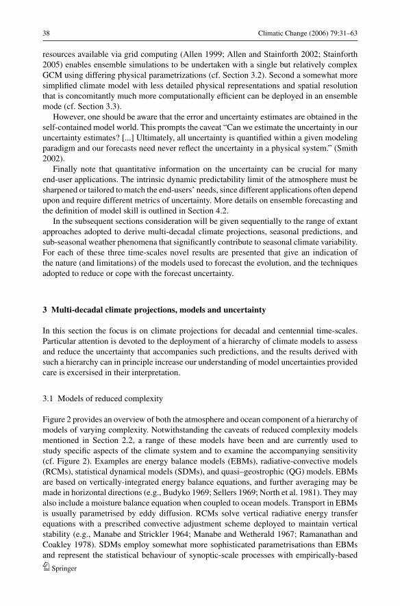
38 Climatic Change (2006) 79:31–63
resources available via grid computing (Allen 1999; Allen and Stainforth 2002; Stainforth2005) enables ensemble simulations to be undertaken with a single but relatively complexGCM using differing physical parametrizations (cf. Section 3.2). Second a somewhat moresimplified climate model with less detailed physical representations and spatial resolutionthat is concomitantly much more computationally efficient can be deployed in an ensemblemode (cf. Section 3.3).
However, one should be aware that the error and uncertainty estimates are obtained in theself-contained model world. This prompts the caveat “Can we estimate the uncertainty in ouruncertainty estimates? [...] Ultimately, all uncertainty is quantified within a given modelingparadigm and our forecasts need never reflect the uncertainty in a physical system.” (Smith2002).
Finally note that quantitative information on the uncertainty can be crucial for manyend-user applications. The intrinsic dynamic predictability limit of the atmosphere must besharpened or tailored to match the end-users’ needs, since different applications often dependupon and require different metrics of uncertainty. More details on ensemble forecasting andthe definition of model skill is outlined in Section 4.2.
In the subsequent sections consideration will be given sequentially to the range of extantapproaches adopted to derive multi-decadal climate projections, seasonal predictions, andsub-seasonal weather phenomena that significantly contribute to seasonal climate variability.For each of these three time-scales novel results are presented that give an indication ofthe nature (and limitations) of the models used to forecast the evolution, and the techniquesadopted to reduce or cope with the forecast uncertainty.
3 Multi-decadal climate projections, models and uncertainty
In this section the focus is on climate projections for decadal and centennial time-scales.Particular attention is devoted to the deployment of a hierarchy of climate models to assessand reduce the uncertainty that accompanies such predictions, and the results derived withsuch a hierarchy can in principle increase our understanding of model uncertainties providedcare is excersised in their interpretation.
3.1 Models of reduced complexity
Figure 2 provides an overview of both the atmosphere and ocean component of a hierarchy ofmodels of varying complexity. Notwithstanding the caveats of reduced complexity modelsmentioned in Section 2.2, a range of these models have been and are currently used tostudy specific aspects of the climate system and to examine the accompanying sensitivity(cf. Figure 2). Examples are energy balance models (EBMs), radiative-convective models(RCMs), statistical dynamical models (SDMs), and quasi–geostrophic (QG) models. EBMsare based on vertically-integrated energy balance equations, and further averaging may bemade in horizontal directions (e.g., Budyko 1969; Sellers 1969; North et al. 1981). They mayalso include a moisture balance equation when coupled to ocean models. Transport in EBMsis usually parametrised by eddy diffusion. RCMs solve vertical radiative energy transferequations with a prescribed convective adjustment scheme deployed to maintain verticalstability (e.g., Manabe and Strickler 1964; Manabe and Wetherald 1967; Ramanathan andCoakley 1978). SDMs employ somewhat more sophisticated parametrisations than EBMsand represent the statistical behaviour of synoptic-scale processes with empirically-based
Springer
Climatic Change (2006) 79:31–63 39
3
Fig. 2 A hierarchy of climate models and their substitutes categorised in terms of resolved spatial dimensionsin atmosphere and ocean components. The names of specific models are given in bold italics. The table isintended to present examples of existing models and is not complete. Abbreviations are explained in the text.Modified from Stocker and Knutti (2003)
relations (e.g., Saltzman 1978). A rigorous approximation to the dynamical equations ismade in QG models (e.g., Gallee et al. 1991; Opsteegh et al. 1998; Hogg et al. 2003).
Examples of ocean model components of reduced complexity are 1-D upwelling-diffusion(UD) models and zonally averaged thermohaline circulation (THC) models (e.g., Marotzkeet al. 1988; Wright and Stocker 1991). Examples of dynamically simplified 3-D models arefrictional geostrophic (FG) models (e.g., Maier-Reimer and Mikolajewicz 1992; Edwardsand Marsh 2005; Muller et al. 2005) and QG models (e.g., Hogg et al. 2003).
In some applications, substitutes of climate models are used that take the form of pulseresponse models. The latter assume a linearity of the response but dramatically increase thecomputational efficiency (Joos and Bruno 1996). Alternatively a neural-network approachformally removes the linearity assumption but does not necessarily replicate the system’snon-linear characteristics (Knutti et al. 2003).
In the next sub-sections we review approaches of assessing uncertainty using models ofdifferent complexity.
3.2 Uncertainty assessment with GCMs
Beyond observational validation of individual models there have been concerted internationalefforts to evaluate the performance of GCMs with model intercomparison projects. Suchprojects involve the coordinated conduct of experiments, and examples include atmosphericGCM simulations with prescribed, historical sea surface conditions (AMIP, cf. Gates et al.1999) and coupled GCM simulations with a historical, scenario, or idealized forcing (CMIP,cf. Covey et al. 2003). These studies reveal the range, similarities and differences in modelbehaviour and help to pinpoint the important processes whose better representation canimprove GCMs. While such an approach is fundamental to capture the structural uncertainty
Springer
40 Climatic Change (2006) 79:31–63
(see type III, Section 2.3), it is not designed to assess parametric uncertainty (the uncertaintyassociated with model parameter values).
Parametric uncertainty was systematically investigated by Murphy et al. (2004) in a singleatmospheric GCM coupled to a mixed-layer ocean model. It involved an ensemble simula-tion of the present-day climate with 53 different model set-ups with 29 key parameters beingvaried separately. The relative reliability of different model set-ups was assessed based onthe deviation of simulated climate from observations. Climate sensitivity (cf. 2.3) was thenestimated by linearly combining the climate feedback parameters, weighted according tothe models’ “diagnosed” reliability. A PDF of climate sensitivity was obtained from ∼106
random combinations of values for the model parameters. With this observational constraintthe 5–95% confidence interval of climate sensitivity narrowed from 1.5–5.3 ◦C to 2.4–5.4 ◦C.However the validity of the linear combination of climate feedback parameters can be ques-tioned (Stainforth 2005), and on the basis of results with a “grand ensemble” of 1000 GCMsimulations a case can be made for a much wider range of climate sensitivity, 1.9−11.5 ◦C. Acaveat is that the latter range was not constrained by observations and hence reflects simplythe a priori PDFs.
Allen et al. (2000) and Stott and Kettleborough (2002) evaluated the uncertainty in predic-tions of future warming by using an empirical linear relationship between the 20th centuryand the mid-21st century warming in models with a hierarchy of complexities. The mid-21stcentury warming is scaled based on the simulated 20th century warming so that the latterbecomes consistent with observations. This scaling was done in a reduced spatio-temporalspace applying optimal fingerprinting (or optimal detection method; cf. Weaver and Zwiers2000; Zwiers 2002). The strength of the method is that the prediction is minimally affectedby the uncertainty in climate sensitivity and ocean heat uptake. In other words, the mod-els are not required to simulate the amplitude of the response accurately, but merely itsstructure. A limitation is that this approach is not applicable if for example the balancebetween GHG and sulphate aerosol forcing changes with time. In addition, the projectiondoes not take into account the abrupt climate change that could result from non-linear ef-fects. Furthermore, the method cannot, by design, account for the forcing uncertainty. Insummary, significant progress has been made during the last few years in the assessment ofuncertainty with GCMs despite the obstacle posed by the severe computational cost of thosemodels.
3.3 Uncertainty assessment with reduced complexity models
3.3.1 Forward modeling to assess uncertainty
To provide a probabilistic “guidance” to the estimates given in Cubasch et al. (2001),Wigley and Raper (2001) assigned, based on IPCC (2001), PDFs to input and model pa-rameters that have large uncertainty: aerosol forcing, climate sensitivity, ocean vertical dif-fusivity, and carbon cycle feedback. The procedure followed was to integrate a UD/EBmodel with various combinations of parameters (∼106 simulations in total) to yield PDFsfor the future temperature change. With an estimated 5–95% confidence interval of warm-ing from 1990 to 2100 the change ranges from 1.7 to 4.9 ◦C. Note however that the de-rived uncertainty range mainly reflects the subjectively determined a priori PDFs of in-put and model parameters, and hence is not an objective quantity. In addition, the absenceof ocean and atmospheric dynamics in the model set-up limits determination of the fulluncertainty.
Springer
Climatic Change (2006) 79:31–63 41
3.3.2 Inverse modeling to assess uncertainty
The application of inversion procedures are common in many geophysical settings. Typicallythey involve the estimate of unknown parameters of a system with given input and output, oran estimate of the input with given system and a known output. For linear systems a directinversion is often possible. However one has to adopt the approach of indirect inversion if thesystem is non-linear (e.g. the climate system), or if neither the input nor parameters are known(e.g. sulphate aerosol forcing and ocean mixing parameters). In a climate modelling settingthis entails adjusting the unknown parameter values to minimise the residuals ( – differencebetween the simulated and observed values) by repeatedly performing forward simulations.In effect observations are used to constrain the range of unknown or uncertain parametersusing the so-called Bayesian approach. This approach requires, by design, a large numberof ensemble members, and current computational cost prohibits its application to coupledGCMs. An example with a reduced complexity model will be given later (Section 3.4).
Recently, several studies with different types of reduced complexity models exploitedthe inverse approach to assess the uncertainty associated with radiative forcing, climatesensitivity, and ocean mixing. Andronova and Schlesinger (2001) used a similar type ofmodel as Wigley and Raper (2001), and conducted ∼104 simulations. Using mean andinterhemispheric difference in near-surface air temperature as constraining variables, theestimated 5–95% confidence interval for total sulphate aerosol forcing and climate sensitivityrange from −0.54 to −0.13 Wm−2 and 1.0 to 9.3 ◦C, respectively. Forest et al. (2002) useda zonally averaged 2-D SDM coupled to a mixed-layer ocean model in which temperatureanomalies diffused into the deep ocean, and conducted ∼101 simulations. Using latitude-height air temperature, and global mean near-surface air temperature and ocean heat uptake asthe constraining variables, the estimated 5–95% confidence intervals for total anthropogenicaerosol forcing, climate sensitivity, and effective ocean diffusivity range from −0.3 to 0.95Wm−2, 1.4 to 7.7 ◦C, and 1.8 × 10⁻⁴ to 56.0 × 10⁻⁴ m2s−1, respectively. Knutti et al. (2002)used a similar model as Stocker and Schmittner (1997), and conducted ∼104 simulations.Using global mean observational records of both near-surface air temperature and oceanheat uptake as constraining variables, their estimated 5–95% confidence interval for indirectaerosol forcing ranges from −1.2 to 0 Wm−2. The a priori uncertainty range for climatesensitivity from 1 to 10 ◦C was not narrowed. The number of ensemble members can beincreased to the order of ∼106 by introducing a neural network to serve as a model substitute(Knutti et al. 2003). Noting that indirect aerosol forcing has the largest uncertainty amongradiative forcing agents, the results of the latter studies constitute a reduction in the uncertaintyof this effect in comparison to the forward modeling approach (Anderson et al. 2003a).However these studies do not place a strong constraint upon the climate sensitivity and thevalue of the ocean mixing parameter with the given large uncertainties in forcing.
3.3.3 Ensemble kalman filtering
As noted earlier there are large uncertainties associated with the representation of unresolvedprocesses in climate models. Annan et al. (2005) and Hargreaves et al. (2004) applied a dataassimilation technique with an ensemble Kalman filter to derive an objective estimate ofuncertainty in parameters of a 3-D FG ocean model coupled to a 2-D EBM. In the usualdata assimilation framework, state variables such as temperature and salinity were adjustedto minimise the difference between simulations and observations (i.e. the residuals) at everyassimilation point. This adjustment results in state variables ‘approaching’ observations. Therelation between model parameter values and the residuals were obtained by conducting
Springer
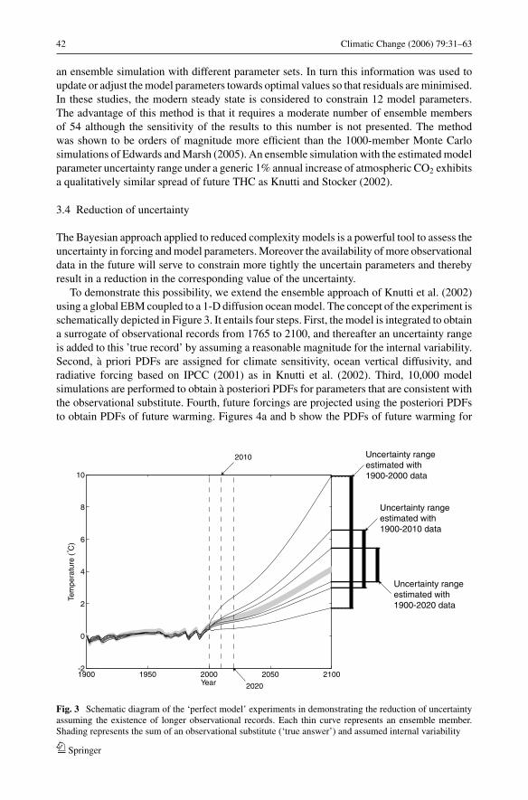
42 Climatic Change (2006) 79:31–63
an ensemble simulation with different parameter sets. In turn this information was used toupdate or adjust the model parameters towards optimal values so that residuals are minimised.In these studies, the modern steady state is considered to constrain 12 model parameters.The advantage of this method is that it requires a moderate number of ensemble membersof 54 although the sensitivity of the results to this number is not presented. The methodwas shown to be orders of magnitude more efficient than the 1000-member Monte Carlosimulations of Edwards and Marsh (2005). An ensemble simulation with the estimated modelparameter uncertainty range under a generic 1% annual increase of atmospheric CO2 exhibitsa qualitatively similar spread of future THC as Knutti and Stocker (2002).
3.4 Reduction of uncertainty
The Bayesian approach applied to reduced complexity models is a powerful tool to assess theuncertainty in forcing and model parameters. Moreover the availability of more observationaldata in the future will serve to constrain more tightly the uncertain parameters and therebyresult in a reduction in the corresponding value of the uncertainty.
To demonstrate this possibility, we extend the ensemble approach of Knutti et al. (2002)using a global EBM coupled to a 1-D diffusion ocean model. The concept of the experiment isschematically depicted in Figure 3. It entails four steps. First, the model is integrated to obtaina surrogate of observational records from 1765 to 2100, and thereafter an uncertainty rangeis added to this ’true record’ by assuming a reasonable magnitude for the internal variability.Second, a priori PDFs are assigned for climate sensitivity, ocean vertical diffusivity, andradiative forcing based on IPCC (2001) as in Knutti et al. (2002). Third, 10,000 modelsimulations are performed to obtain a posteriori PDFs for parameters that are consistent withthe observational substitute. Fourth, future forcings are projected using the posteriori PDFsto obtain PDFs of future warming. Figures 4a and b show the PDFs of future warming for
1900 1950 2000 2050 2100-2
0
2
4
6
8
10
Year
Tem
pera
ture
(° C
)
2010
2020
Uncertainty rangeestimated with1900-2000 data
Uncertainty rangeestimated with1900-2010 data
Uncertainty rangeestimated with1900-2020 data
Fig. 3 Schematic diagram of the ‘perfect model’ experiments in demonstrating the reduction of uncertaintyassuming the existence of longer observational records. Each thin curve represents an ensemble member.Shading represents the sum of an observational substitute (‘true answer’) and assumed internal variability
Springer
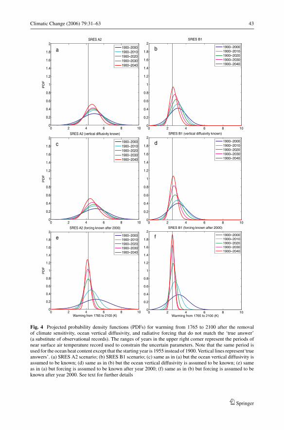
Climatic Change (2006) 79:31–63 43
0 2 4 6 8 100
0.2
0.4
0.6
0.8
1
1.2
1.4
1.6
1.8
2P
DF
SRES A2
a 1900–20001900–20101900–20201900–20301900–2040
0 2 4 6 8 100
0.2
0.4
0.6
0.8
1
1.2
1.4
1.6
1.8
2SRES B1
b 1900–20001900–20101900–20201900–20301900–2040
0 2 4 6 8 100
0.2
0.4
0.6
0.8
1
1.2
1.4
1.6
1.8
2
PD
F
SRES A2 (vertical diffusivity known)
c 1900–20001900–20101900–20201900–20301900–2040
0 2 4 6 8 100
0.2
0.4
0.6
0.8
1
1.2
1.4
1.6
1.8
2SRES B1 (vertical diffusivity known)
d 1900–20001900–20101900–20201900–20301900–2040
0 2 4 6 8 100
0.2
0.4
0.6
0.8
1
1.2
1.4
1.6
1.8
2
Warming from 1765 to 2100 (K)
PD
F
SRES A2 (forcing known after 2000)
e 1900–20001900–20101900–20201900–20301900–2040
0 2 4 6 8 100
0.2
0.4
0.6
0.8
1
1.2
1.4
1.6
1.8
2
Warming from 1765 to 2100 (K)
SRES B1 (forcing known after 2000)
f 1900–20001900–20101900–20201900–20301900–2040
Fig. 4 Projected probability density functions (PDFs) for warming from 1765 to 2100 after the removalof climate sensitivity, ocean vertical diffusivity, and radiative forcing that do not match the ‘true answer’(a substitute of observational records). The ranges of years in the upper right corner represent the periods ofnear surface air temperature record used to constrain the uncertain parameters. Note that the same period isused for the ocean heat content except that the starting year is 1955 instead of 1900. Vertical lines represent‘trueanswers’. (a) SRES A2 scenario; (b) SRES B1 scenario; (c) same as in (a) but the ocean vertical diffusivity isassumed to be known; (d) same as in (b) but the ocean vertical diffusivity is assumed to be known; (e) sameas in (a) but forcing is assumed to be known after year 2000; (f) same as in (b) but forcing is assumed to beknown after year 2000. See text for further details
Springer
44 Climatic Change (2006) 79:31–63
scenarios SRES A2 and B1, respectively. PDFs narrow moderately with the use of longerobservational records.
Figures 4c and d show the results subject to the assumption of perfect knowledge of oceanvertical diffusivity. The results exhibit few differences from Figures 4a and b, implying thatthe impact of the uncertainty in ocean vertical diffusivity on temperature changes is smallrelative to other uncertainties. Figures 4e and f show the results when we assume perfectknowledge of radiative forcing after the year 2000. Here the results narrow dramaticallythe PDFs and thereby reduce the uncertainty range. This result points to the importanceto focus efforts in quantifying the radiative forcing for the next decades. The figures alsoreveal that PDFs are biased from true values when the parameters are not well constrainedby observations (cf. Figure 3).
Another possible avenue of future research is to increase the number of variables to furtherconstrain uncertainty parameters. For example recent observational studies (Curry et al. 2003)showed that the anthropogenic signal is evident in the salinity field in the Atlantic Oceanduring the past four decades. This suggests that the salinity field could serve as a potentialconstraint.
Here the focus was on estimating the uncertainty of climate projections. Next, we continueto address probabilistic methods and introduce quantitative statistical measures of forecastuncertainty, with a specific focus on the interface to operational application and the end-userperspective. This will be exemplified on the seasonal time-scale.
4 Seasonal climate prediction
4.1 The rationale
A major addition to the forecasting repertoire of weather services in recent years has beenthe development of operational techniques for seasonal climate predictions. It is argued thatsustained large-scale surface (ocean and land-surface) forcing can exert a coherent and con-ceivably predictable atmospheric response on seasonal time-scales. Indeed the atmosphereitself exhibits coherent large-scale climate variations on this time-scale. Likewise it has beensuggested that well-recognised atmospheric flow phenomena or features that are confined tospecific regions/layers but that are sustained on quasi-seasonal time-scales can influence theseasonal patterns in the far-field. Two possible examples are the equatorially-based Madden-Julian Oscillation and the stratospheric polar annular oscillation.
Seasonal forecasts are derived using either statistical or dynamical models or a combi-nation (for an overview see Goddard et al. 2003). In practice elements of the statistical anddynamical approaches are combined in a seasonal forecasting system (e.g., Palmer et al.2005). For example a serial approach utilises a statistical model to generate oceanic bound-ary conditions for the atmospheric dynamical model (Colman and Davey 2003). Likewise theoutput of dynamical models can be subject to statistical post-processing to compensate formodel drift or to counter known limitations such as resolution. Such a model calibration re-quires an adequate number of forecasts performed from initial states in the past (“hindcasts”).Most dynamical models or hybrid forecasting systems based upon a mix of statistical and dy-namical ingredients exhibit a low signal-to-noise ratio.4 Hence the desire to derive estimatesof forecast uncertainty in the probabilistic framework (Palmer 1993).
4 Ratio of the variability related to external forcing and the unpredictable part of internal variability.
Springer
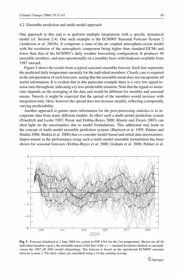
Climatic Change (2006) 79:31–63 45
4.2 Ensemble prediction and multi-model approach
One approach to this end is to perform multiple integrations with a specific dynamicalmodel (cf. Section 2.4). One such example is the ECMWF Seasonal Forecast System 2(Anderson et al. 2003b). It comprises a state-of-the-art coupled atmosphere-ocean modelwith the resolution of the atmospheric component being higher than standard GCMs andlower than that of the ECMWF’s daily weather forecasting configuration. It produces 40ensemble members, and runs operationally on a monthly basis with hindcasts available from1987 onward.
Figure 5 shows the results from a typical seasonal ensemble forecast. Each line representsthe predicted daily temperature anomaly for the individual members. Clearly care is requiredin the interpretation of such forecasts, noting that the ensemble mean does not encapsulate alluseful information. It is evident that in this particular example there is a very low signal-to-noise ratio throughout, indicating a ly less-predictable situation. Note that the signal-to-noise-ratio depends on the averaging of the data and would be different for monthly and seasonalmeans. Naively it might be expected that the spread of the members would increase withintegration time. Here, however the spread does not increase steadily, reflecting a temporallyvarying predictability.
Another approach to garner more information for the post-processing statistics is to in-corporate data from many different models. In effect such a multi-model prediction system(Fraedrich and Leslie 1987; Pavan and Doblas-Reyes 2000; Kharin and Zwiers 2003) canshed light on the uncertainties due to model formulations. This additional step leads tothe concept of multi-model ensemble prediction systems (Harrison et al. 1995; Palmer andShukla 2000; Shukla et al. 2000) that co-consider model-based and initial data uncertainties.Improvement in the performance using such a multi-model ensemble formulation has beenshown for seasonal forecasts (Doblas-Reyes et al. 2000; Graham et al. 2000; Palmer et al.
Fig. 5 Forecast initialized at 1 June 2004 for a point in NW-USA for the 2 m temperature. Shown are all 40individual members (grey), the ensemble mean (solid line) with +/− standard deviation (dashed) as anomalyversus the 1987 till 2001 model climatology. The forecast is based on the operational ECMWF seasonalforecast system 2. The daily values are smoothed using a 14 day running average
Springer
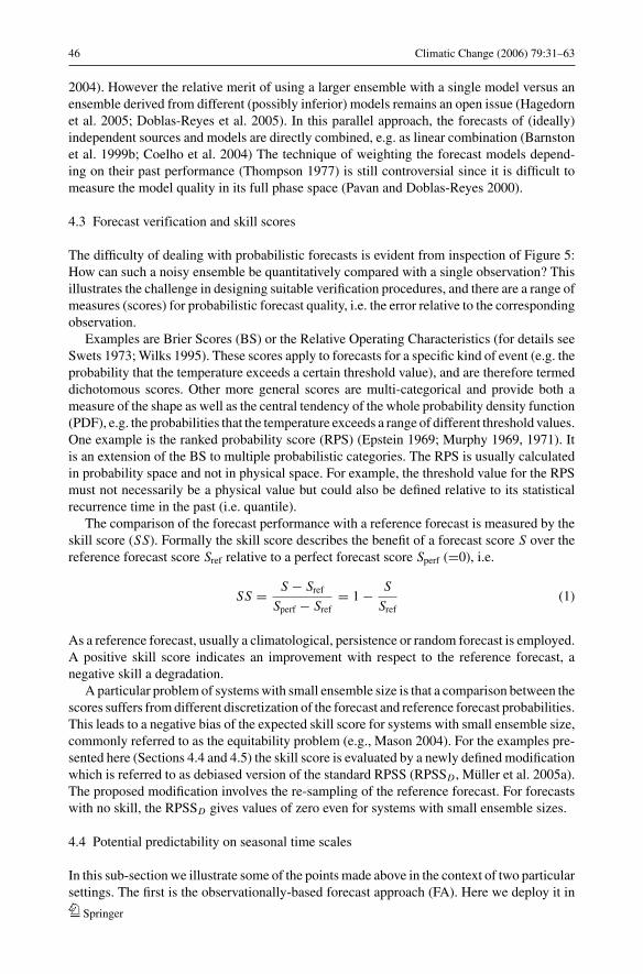
46 Climatic Change (2006) 79:31–63
2004). However the relative merit of using a larger ensemble with a single model versus anensemble derived from different (possibly inferior) models remains an open issue (Hagedornet al. 2005; Doblas-Reyes et al. 2005). In this parallel approach, the forecasts of (ideally)independent sources and models are directly combined, e.g. as linear combination (Barnstonet al. 1999b; Coelho et al. 2004) The technique of weighting the forecast models depend-ing on their past performance (Thompson 1977) is still controversial since it is difficult tomeasure the model quality in its full phase space (Pavan and Doblas-Reyes 2000).
4.3 Forecast verification and skill scores
The difficulty of dealing with probabilistic forecasts is evident from inspection of Figure 5:How can such a noisy ensemble be quantitatively compared with a single observation? Thisillustrates the challenge in designing suitable verification procedures, and there are a range ofmeasures (scores) for probabilistic forecast quality, i.e. the error relative to the correspondingobservation.
Examples are Brier Scores (BS) or the Relative Operating Characteristics (for details seeSwets 1973; Wilks 1995). These scores apply to forecasts for a specific kind of event (e.g. theprobability that the temperature exceeds a certain threshold value), and are therefore termeddichotomous scores. Other more general scores are multi-categorical and provide both ameasure of the shape as well as the central tendency of the whole probability density function(PDF), e.g. the probabilities that the temperature exceeds a range of different threshold values.One example is the ranked probability score (RPS) (Epstein 1969; Murphy 1969, 1971). Itis an extension of the BS to multiple probabilistic categories. The RPS is usually calculatedin probability space and not in physical space. For example, the threshold value for the RPSmust not necessarily be a physical value but could also be defined relative to its statisticalrecurrence time in the past (i.e. quantile).
The comparison of the forecast performance with a reference forecast is measured by theskill score (SS). Formally the skill score describes the benefit of a forecast score S over thereference forecast score Sref relative to a perfect forecast score Sperf (=0), i.e.
SS = S − Sref
Sperf − Sref= 1 − S
Sref(1)
As a reference forecast, usually a climatological, persistence or random forecast is employed.A positive skill score indicates an improvement with respect to the reference forecast, anegative skill a degradation.
A particular problem of systems with small ensemble size is that a comparison between thescores suffers from different discretization of the forecast and reference forecast probabilities.This leads to a negative bias of the expected skill score for systems with small ensemble size,commonly referred to as the equitability problem (e.g., Mason 2004). For the examples pre-sented here (Sections 4.4 and 4.5) the skill score is evaluated by a newly defined modificationwhich is referred to as debiased version of the standard RPSS (RPSSD , Muller et al. 2005a).The proposed modification involves the re-sampling of the reference forecast. For forecastswith no skill, the RPSSD gives values of zero even for systems with small ensemble sizes.
4.4 Potential predictability on seasonal time scales
In this sub-section we illustrate some of the points made above in the context of two particularsettings. The first is the observationally-based forecast approach (FA). Here we deploy it in
Springer
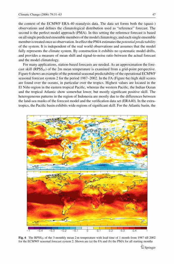
Climatic Change (2006) 79:31–63 47
the context of the ECMWF ERA-40 reanalysis data. The data set forms both the (quasi-)observations and defines the climatological distribution used as “reference” forecast. Thesecond is the perfect model approach (PMA). In this setting the reference forecast is basedon all single predicted ensemble members of the model climatology, and each single ensemblemember is treated once as observation. In effect the PMA estimates the potential predictabilityof the system. It is independent of the real world observations and assumes that the modelfully represents the climate system. By construction it exhibits no systematic model drifts,and provides a measure of mean shift and signal-to-noise ratio between the actual forecastand the model climatology.
For many applications, station-based forecasts are needed. As an approximation the fore-cast skill (RPSSD) of the 2m mean temperature is examined from a grid-point perspective.Figure 6 shows an example of the potential seasonal predictability of the operational ECMWFseasonal forecast system 2 for the period 1987–2002. In the FA (Figure 6a) high skill scoresare found over the oceans, in particular over the tropics. Highest values are located in theEl Nino region in the eastern tropical Pacific, whereas the western Pacific, the Indian Oceanand the tropical Atlantic show somewhat lower, but mostly significant positive skill. Theheterogeneous patterns in the region of Indonesia are mostly due to the differences betweenthe land-sea masks of the forecast model and the verification data set (ERA40). In the extra-tropics, the Pacific basin exhibits wide regions of significant skill. For the Atlantic basin, the
Fig. 6 The RPSSD of the 3-monthly mean 2 m temperature with lead time of 1 month from 1987 till 2002for the ECMWF seasonal forecast system 2. Shown are (a) the FA and (b) the PMA for all starting months
Springer
48 Climatic Change (2006) 79:31–63
values are closer to zero. Relevant for Europe, there is a band-like structure of a weak positivesignal across the northern Atlantic reaching from Newfoundland to the Bay of Biscay. Overland, the skills are lower throughout. Highest values are found over Northern America, andalong the Pacific coast of Asia. Most other continents, in particular Europe, are associatedwith negative or non-significant values.
The potential predictability estimated by the PMA supports these findings (Figure 6b).The tropical oceans feature high potential predictability. In the extratropics, the oceans showreduced but still significant positive values. Over land, the PMA implies a higher predictabilityin the tropics than extratropics (e.g. over Africa and Southern America). A comparison to theFA shows, that this potential is not realised in the actual forecast skill. A better agreementbetween PMA and FA is found in the extratropics with very limited, but significant, skillvalues. In particular over the European region the skill scores are in the order of less then10%, both for PMA and FA.
4.5 Forecasting climate indices (ENSO and NAO)
Accurate extended-range predictions of regional and global climate indices are highly de-sirable in the context of impact research and applications. Here we discuss and compare theforecast skills for the ENSO and NAO index.
Coupled atmosphere-ocean models as well as statistical models yield a significant positivelevel of forecast skill for ENSO up to a lead time of 12 months (for a review see Latif et al.1998). The predictions depend critically on the phase of the ENSO (Fedorov 2002; Vitartet al. 2003; McPhaden 2004). In a comparative study of the forecast for the 1997/98 El Nino,Landsea and Knaff (2000) examined 12 deterministic statistical and dynamical models andfound no skill beyond persistence on seasonal to inter-annual time scales for any model. Moregenerally, van Oldenborgh et al. (2003) compared the ECMWF seasonal forecast system 1and 2 (Anderson et al. 2003b) against a statistical and a persistence model of the form of Knaffand Landsea (1997) for the full period 1987–2001. In terms of skill, the statistical methodsperform similar to the dynamical models in the winter months. However, in the summermonths the skill scores of the statistical models are strongly reduced (“spring barrier”).Among all models, the lowest skill score is achieved by the persistence model in the summermonths.
For the NAO, operational statistical and more recently dynamical forecasting systemssuggest only moderate skill. The statistical properties of the time series enables statisticalforecasts based directly on the time series (Stephenson et al. 2000). Other efforts have focusedon the role of the Atlantic SST (Czaja and Frankignoul 1999, 2002; Peng et al. 2003), Eurasiansnow cover (Cohen and Entekhabi 1999) and more recently the lower stratosphere (Baldwinand Dunkerton 2001; Baldwin et al. 2003). Recent modeling studies (Rodwell et al. 1999;Rodwell and Folland 2002) and statistical approaches (Saunders and Qian 2002) provideenhanced forecast skill with preceding summer/autumn SST. However, some authors explainthe skill as a statistical artefact (Bretherton and Battisti 2000). Several studies investigatedynamical systems on the skill of NAO predictions (Doblas-Reyes et al. 2003; Muller et al.2005b) and find very limited, but positive, skill values. Other large-scale variability patternsin the Euro-Atlantic sectors exhibit higher predictability, probably due to a more direct oceanforcing (Pavan et al. 2000a,b).
As an illustration, the skill for ENSO and NAO forecasts is calculated for the ECMWFseasonal forecasts system 2 (Figure 7). For the NAO, the skill scores are much lower thanfor the ENSO forecasts, with values of around 25% for the FA and much lower (8%) forPMA. Both values are statistically significant as derived using a Monte Carlo approach. This
Springer
Climatic Change (2006) 79:31–63 49
ENSO NAO
0.0
0.2
0.4
0.6
0.8
1.0
ERA40 PMA 0.0
0.2
0.4
0.6
0.8
1.0
ERA40 PMA
Fig. 7 The RPSSD of (a) ENSOand (b) NAO index for winter(DJF) averages from 1987 till2001 for the ECMWF seasonalforecast system 2 started atNovember 1st. The verification isundertaken in the FA (light grey)and the PMA (black). Thehorizontal red lines denote thestatistical significance level of95%
indicates that the potential predictability of this climate pattern is lower than the actuallyachieved skill over this period. Indeed, skill scores of this magnitude are very sensitive to thesample size and the NAO skill mainly originates from a few well-predicted events (Doblas-Reyes et al. 2003; Muller et al. 2005b). The limited number of available hindcasts for theoperational ECMWF system 2 (15 years) is a major constraint for the verification.
The intra-seasonal dynamics of the above patterns of climate variability is at the heart ofthe following Section 5.
5 Patterns of intra-seasonal variability and weather regimes
5.1 The rationale
The regional impact of climate change is communicated through the leading modes of climatevariability. To assess their behaviour under future climate change and to quantify the reliabilityof climate projections it is necessary to identify the dynamical and physical mechanisms thatunderly climate variability (Sutton 2005).
As indicated in Section 2.1, weather regimes such as atmospheric blocking, can have asignificant impact on the patterns of inter-annual variability. This is supported by their largepersistence of ∼10 days; their spatial extent (O(106) km2); and their significant disturbanceto the ambient climatic conditions. In effect blocking systems are associated with a reductionof the in-situ zonal wind, and a deflection of transient cyclonic systems away from theircustomary tracks with an accompanying marked redistribution of precipitation (Rex 1950a,b, Trigo et al. 2004). Hence the correct prediction of intra-annual and intra-seasonalvariability and the associated uncertainty hinges to some extent on the predictability ofthe blocking phenomenon. The processes involved in blocking formation are complex andoccur on a range of scales (see later), and their correct prediction, particularly their onsetand breakdown remains difficult (Anderson 1993; D’Andrea et al. 1998; Oortwijn 1998).
It is therefore instructive: to consider the relation between blocking and modes of climatevariability; to explore the cause-and-effect relationship between blocking and regional climatepatterns; and to review some of the notions on the underlying dynamics of blocking, thatmight be crucial for the correct representation of blocking in models.
Springer
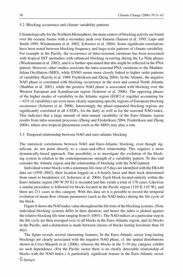
50 Climatic Change (2006) 79:31–63
5.2 Blocking occurrence and climate variability patterns
Climatologically for the Northern Hemisphere, the main centers of blocking activity are foundover the oceanic basins with a secondary peak over Eurasia (Sausen et al. 1995; Lupo andSmith 1995; Wiedenmann et al. 2002; Schwierz et al. 2004). Some significant correlationshave been noted between blocking frequency and large-scale patterns of climate variability.For example in the Pacific, the occurrence of intra-seasonal variations has been associatedwith tropical SST anomalies with enhanced blocking occurring during the La Nina phases(Wiedenmann et al. 2002), and it is further speculated that this might be reflected in the PNApattern. However, other studies associate the intra-seasonal PNA variations to the Madden-Julian Oscillation (MJO), while ENSO seems more closely linked to higher order patternsof variability (Karoly et al. 1989; Frederiksen and Zheng 2004). In the Atlantic, the negativeNAO phase is correlated with blocking occurrence in the west and central North Atlantic(Shabbar et al. 2001), while the positive NAO phase is associated with blocking over theWestern European and Scandinavian region (Scherrer et al. 2006). The opposing phasesof the higher modes of variability in the Atlantic region (EOF2-4, together accounting for∼42% of variability) are even more clearly separating specific regions of European blockingoccurrence (Scherrer et al. 2006). Interestingly the phase-separated blocking regions aresignificantly correlated in all 4 EOFs, for the daily as well as for the seasonal NAO-index.This indicates that a large amount of inter-annual variability of the Euro-Atlantic regionresults from intra-seasonal processes (Zheng and Frederiksen 2004; Frederiksen and Zheng2004), where also tropical phenomena (such as the MJO) may play a role.
5.3 Temporal relationship between NAO and euro-atlantic blocking
The statistical correlations between NAO and Euro-Atlantic blocking, even though sig-nificant, do not point directly to a cause-and-effect relationship. This requires a moredynamically-based approach. One possibility is to investigate the evolution of the block-ing system in relation to the contemporaneous strength of a variability pattern. To this endconsider the Atlantic region and the relationship of blocking with the NAO pattern.
Individual winter blocks with a minimum life-time of 5 days are identified with the ERA40data set (1958–2002), their location logged on a 6-hourly basis and their track determinedfrom onset to breakdown (cf. Schwierz et al. 2004). Each block located entirely within theEuro-Atlantic region [90◦W:50◦E] is recorded and this yields a total of 178 cases. Likewisea similar procedure is followed for blocks located in the Pacific region [110◦E:110◦W], andthere are 211 cases in this category. With this data set it is possible to record the temporalevolution of mean-flow climate parameters (such as the NAO index) during the life cycle ofthe block.
Figure 8 shows the NAO index value throughout the life time of the blocking systems. (Noteindividual blocking systems differ in their duration, and hence the index is plotted againstthe relative blocking life time ranging from 0–100%). The NAO indices at a particular step inthe life cycle are then averaged over (i) all blocks in the Euro-Atlantic region, and (ii) blocksin the Pacific, and a distinction is made between classes of blocks lasting less/more than 10days.
The figure reveals several interesting features. In the Euro-Atlantic sector long-lastingblockings are clearly associated with the negative NAO phase, cf. the spatial distributionsshown in Croci-Maspoli et al. (2006), whereas the blocks in the 5–10 day category exhibitno such dependence. (For the Pacific sector there is no clearly detectable relationship ofblocks with the NAO index.) A particularly significant feature in the Euro-Atlantic sector
Springer
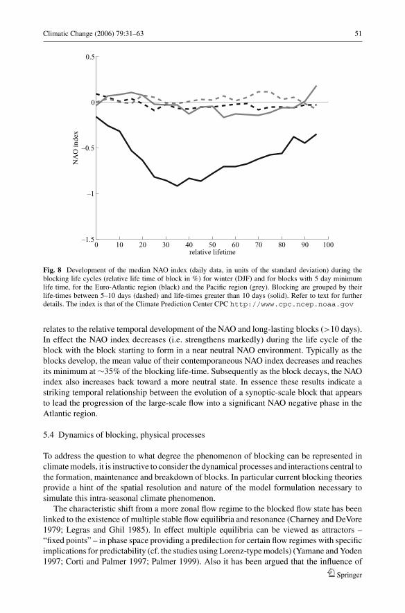
Climatic Change (2006) 79:31–63 51
0 10 20 30 40 50 60 70 80 90 100–1.5
–1
–0.5
0
0.5
relative lifetime
NA
O in
dex
Fig. 8 Development of the median NAO index (daily data, in units of the standard deviation) during theblocking life cycles (relative life time of block in %) for winter (DJF) and for blocks with 5 day minimumlife time, for the Euro-Atlantic region (black) and the Pacific region (grey). Blocking are grouped by theirlife-times between 5–10 days (dashed) and life-times greater than 10 days (solid). Refer to text for furtherdetails. The index is that of the Climate Prediction Center CPC http://www.cpc.ncep.noaa.gov
relates to the relative temporal development of the NAO and long-lasting blocks (>10 days).In effect the NAO index decreases (i.e. strengthens markedly) during the life cycle of theblock with the block starting to form in a near neutral NAO environment. Typically as theblocks develop, the mean value of their contemporaneous NAO index decreases and reachesits minimum at ∼35% of the blocking life-time. Subsequently as the block decays, the NAOindex also increases back toward a more neutral state. In essence these results indicate astriking temporal relationship between the evolution of a synoptic-scale block that appearsto lead the progression of the large-scale flow into a significant NAO negative phase in theAtlantic region.
5.4 Dynamics of blocking, physical processes
To address the question to what degree the phenomenon of blocking can be represented inclimate models, it is instructive to consider the dynamical processes and interactions central tothe formation, maintenance and breakdown of blocks. In particular current blocking theoriesprovide a hint of the spatial resolution and nature of the model formulation necessary tosimulate this intra-seasonal climate phenomenon.
The characteristic shift from a more zonal flow regime to the blocked flow state has beenlinked to the existence of multiple stable flow equilibria and resonance (Charney and DeVore1979; Legras and Ghil 1985). In effect multiple equilibria can be viewed as attractors –“fixed points” – in phase space providing a predilection for certain flow regimes with specificimplications for predictability (cf. the studies using Lorenz-type models) (Yamane and Yoden1997; Corti and Palmer 1997; Palmer 1999). Also it has been argued that the influence of
Springer
52 Climatic Change (2006) 79:31–63
topography upon the zonal mean flows can destabilise the flow and lead the system to oscillatefrom one attractor to another (Haines and Hannachi 1995).
A related group of studies link blocks to the amplification of stationary planetary-scalewaves (Cerlini et al. 1999; Liu 1994; Da Silva and Lindzen 1993; Hansen and Sutera 1993;Nigam and Lindzen 1989), and the importance of non-linear interactions with large-scaletravelling waves has been stressed (Egger 1978). For blocking, the constructive interferenceof land-sea contrast (thermal forcing) and topographic forcing seems to be crucial (Ji andTibaldi 1983; Tung and Lindzen 1979; Egger 1978), and no long-lasting events (>6 days)were possible without mountains in numerical sensitivity experiments (Mullen 1989a). Frommountain torque and angular momentum analyses, Lott et al. (2004a; b) also concluded, thatthe jet streams’ interactions with large-scale topography play a key-role for hemispheric andregional variability on the 20–30-day time-scale.
There is evidence that certain large-scale mechanisms precondition the atmosphere so asto favour blocking formation. Da Silva and Lindzen (1993) and Nigam and Lindzen (1989)showed that the stationary wave amplitude is sensitive to small shifts in the subtropical jetand the sharpness of the jet. Preconditioning by teleconnection patterns involves a tropicaldiabatic vorticity anomaly with a subsequent global-scale Rossby-wave train into the extra-tropics (Hoskins and Karoly 1981; Simmons et al. 1983; Hoskins and Sardeshmukh 1987).
A more local view of blocking maintenance is the so-called eddy-straining hypothesisthat relates to the modification of the mean flow by the eddies (Berggren et al. 1949; Shutts1983; Mullen 1987; Vautard et al. 1988). More recent studies by Tsou and Smith (1990), andLupo and Smith (1995) and others confirm the feedback from eddies to the mean flow in thecase of blocking events.
It has been shown, that moist cloud-diabatic processes induced by transient synopticsystems and orographic forcing can act to maintain blocking anomalies Schwierz (2001).Transient disturbances are also believed to play a crucial role in the onset and breakdown ofthe blocking anomalies. Deep upstream cyclogenesis appears to trigger Atlantic blocking. Jiand Tibaldi (1983), Crum and Stevens (1988), and Lupo and Smith (1995) found a positivecorrelation between the intensity of blocking anticyclones and the intensity of the precursorcyclone development.
It is evident from the above that many components of the climate system potentiallyplay a role in the dynamics of blocking. From a predictability perspective, elements such astopography, cyclones, moist processes, tropical and stratospheric forcings need to be resolvedand represented appropriately.
5.5 Predictability of blocking and climate patterns
Difficulties in forecasting block occurrence might well relate to the intrinsic predictability ofthe associated climate regime. Studies have been undertaken using a range of approaches fromexperiments with state-of-the-art NWP models to probabilistic methods, such as (i) seasonalensemble hindcasts of Euro-Atlantic wintertime variability (Pavan et al. 2000b), (ii) assess-ment of predictability of blocking with ensemble methods (Frederiksen et al. 2004; Mauritsenand Kallen 2004; Pelly and Hoskins 2003; Watson and Colucci 2002), (iii) the multi-modelapproach (Pavan and Doblas-Reyes 2000; Doblas-Reyes et al. 2003) (cf. also Section 4.2),and also (iv) climate simulations and GCM intercomparison projects (Sausen et al. 1995;Tibaldi et al. 1997; D’Andrea et al. 1998; Doblas-Reyes et al. 1998).
Some standard model deficiencies can impact on the prediction of blocks and intra-seasonal variability. For example in GCMs these include: an excessive zonality of jet streams;greater than normal storm track activity and undersimulation of low-frequency planetary and
Springer
Climatic Change (2006) 79:31–63 53
stationary waves. For the prediction of blocks themselves it has been noted that there is: –ageneral tendency to underestimate blocking activity (frequency), particularly for extendedforecast times Jung (2005); –a lack of long-lived blocks (D’Andrea et al. 1998); –a tendencyof Atlantic blocking to be shifted east, since transients penetrate too far east and south asthe jet stream becomes too zonal (Doblas-Reyes et al. 1998) (Pacific blocking predictionsdo not show this tendency). Moreover forecast model errors differ significantly in the skillin representing Pacific and Atlantic blocks (Tibaldi et al. 1994), and indeed the skill of the(ECMWF) seasonal model prediction is higher in the Pacific than in the Atlantic (Pavan et al.2000a). This in turn might betoken the fact that different processes for blocking formationprevail for the two main NH blocking regions.
A regime-dependent component has been found in forecast error fields (Molteni andTibaldi 1990), and the systematic model errors of 500-hPa geopotential height are relatedto the inability to predict blocking (Mauritsen and Kallen 2004). This has ramificationsfor quantifying forecast uncertainty, and in particular the difficulties in correctly predictingthe onset and break-down of blocking periods have profound implications. In the mediumrange, major forecast failures are associated with regime transitions, that affect the statisticalproperties of the errors (Trevisan et al. 2001).
For long-range or seasonal prediction, the presumed linkage of sea-surface temperature(SST) anomalies to patterns of climate variability and blocking is noteworthy and relatesto the paradigm of preconditioning the atmosphere towards specific regimes of variability.Earlier studies hinted at the impact of Pacific SST anomalies on blocking location (Mullen1989b). In the North Pacific, low-frequency (blocking) variability is enhanced during LaNina winters and hence potential predictability during El Nino winters is increased (Chenand van den Dool 1999). Using GCM experiments, Cassou et al. (2004) and Mathieu et al.(2004) find that tropical and extra-tropical Atlantic SST anomalies can significantly affect theexcitation of North Atlantic climate regimes such as the NAO and blocking. The influence ofENSO-modulated SST anomalies on Euro-Atlantic blocking can be limited by the model’sability to correctly represent planetary wave propagation from the Pacific into the Atlantic(Pavan et al. 2000b).
5.6 Further comments and challenges
In this section we have emphasised the issue of predictability and illustrated the challenge ofclimate variability prediction from a process-based standpoint. The range and interaction ofprocesses and the need to represent them sufficiently accurately is a major difficulty for predic-tion. Here this was pinpointed in the context of the need for a better fundamental understandingof the synoptic processes underlying the onset, maintenance and breakdown of blocks (sic.weather regimes) and their non-linear two-way interaction with the pattern of climate-scalevariability.
For example the co-development of an individual blocking event and a negative NAOphase has been shown to be linked to the life time of the block. The implication is that amodel should adequately represent the processes relevant for blocking (wave interactions,diabatic heating, interactions with the ocean or stratosphere).
Sensitivity studies with climate models of parameters such as resolution, physicalparametrisation, moisture content, surface schemes, representation of ocean and tropicalprocesses might help to investigate the link between predictability of climate and weatherregimes. And indeed there are indications that some of the model errors for blocking canbe alleviated by increased resolution (Doblas-Reyes et al. 1998) and improvements in thephysical parametrisation (Molteni and Tibaldi 1990).
Springer
54 Climatic Change (2006) 79:31–63
6 Final remarks
A major difficulty in predictions and the assessment of uncertainty is the determinationand separation of influencing factors on climate variability and change. These comprise aforced component (GHGs), internal sources (such as QBO, NAO, PNA, ENSO, feedbackwith eddies), residual weather “noise” and their non-linear interactions.
It has been argued here that a hierarchy of models is a powerful approach to estimateand assess the uncertainty. Dynamical models have been combined with models of reducedcomplexity, and with statistical models. Beneficial for the assessment is an overlap betweenthe model evaluations. For instance models used in NWP can be combined with GCMsfor climate and seasonal time scales to determine the accurate representation of processes(Section 5). Such GCMs in connection with reduced-complexity and statistical models,which are often used in an ensemble mode, are efficient in the estimation of errors. Inaddition such an overlap can lend credence to the applicability of the less-detailed models(cf. Section 3). However, long-term projections – in particular when undertaken withstatistical models – rely on assumptions such as stationarity and ergodicity which are notfulfilled for instance for dramatic changes in circulation patterns. (cf. Section 2). Climatemodels, especially with reduced complexity and relaxed non-linearity, will not necessarilyforesee a major change in dominant circulation regimes (Smith 2002).
6.1 Internal, natural, and regional variability
Hence, the application of a model hierarchy is also beset with problems. In climate studies,the internal variability of the climate system sets a level of background noise to attempts toestimate or predict an external or anthropogenic signal (Manabe and Stouffer 1996; Stoufferet al. 2000). A prediction by a single climate simulation or any parameter estimation thatuses observational records as a constraint is subject to the uncertainties due to this internalvariability and stochastic uncertainties (Murphy et al. 2004). These uncertainties are expectedto increase if one goes to regional scales.
It has been argued that the externally forced signal may be preferentially projected ontothe existing large scale modes of variability inherent in the climate system by changing theprobability distribution of weather regimes (Palmer 1998, 1999; Corti et al. 1999; Monahanet al. 2000). Considering the impact of these large scale modes of variability on regionalclimate (Hurrell 1995, 1996; Thompson and Wallace 2001) as well as on the THC (Latif et al.2000; Delworth and Dixson 2000; Schmittner et al. 2000), the understanding of underlyingmechanisms of internal variability is important for (i) the justification of the choice of a modelof reduced complexity and (ii) the extension of uncertainty assessment toward regional scales.In addition, the spatial inhomogeneity of radiative forcing, e.g. by tropospheric aerosols,which is represented as a globally uniform radiative forcing in reduced complexity models,may have a non-negligible impact on regional-scale climate change.
6.2 Reduced complexity models
The potential utility of a reduced complexity models is enhanced if its response overlaps andreplicates that of comprehensive model. An example of such an overlap is the projection offuture changes in the thermohaline circulation (THC). The fate of the THC in a warmingworld has attracted considerable attention due to its significant global and regional impact.Stocker and Schmittner (1997) used a multi-basin, zonally-averaged ocean model coupledto a 1-D EBM and conducted a series of experiments with different boundary conditions.
Springer
Climatic Change (2006) 79:31–63 55
They found that the reduction of the THC depends on the rate of increase in GHG forcing. Asimilar result, albeit in a much smaller parameter space, was derived with a 3-D fully coupledGCM (Stouffer and Manabe 1999). The THC system is highly nonlinear, and hence a largenumber of ensemble members are necessary to obtain a robust picture. Indeed, many GCMsproject quite different strengths of the future THC (as well as modern simulations). Knuttiand Stocker (2002), using a similar model as Stocker and Schmittner (1997), conducted anensemble of 100 simulations with different noise sequences which represent the atmosphericinternal variability. For that particular model setting they showed that the predictability ofTHC is severely limited when the system approaches the instability threshold or bifurcationpoint.
6.3 Structural uncertainty
GCMs, albeit expensive, are believed to be better suited for the use in projections of futureclimate change. However, reduced complexity models are very useful to assess uncertaintywith probabilistic representations and ensemble methods. It is also possible for those mod-els to objectively optimise the model parameter values, and hence reduce the parametricuncertainties. For reduced complexity models to serve as GCM substitutes, it is desirableto direct more effort towards the structural uncertainties. It remains a challenge to assesshow much uncertainty or error could be introduced by reducing the complexity of models.Of course, structural uncertainty does not only exist in reduced complexity models but alsoin GCMs. With regard to THC projections, for example, these are poor representation ofwestern boundary currents, deep convection, and flow over shallow sills. It is hoped thatthese weaknesses in GCMs are continuously improved as our understanding on fundamentalprocesses and computational power increase. A hierarchy of climate models is useful andnecessary, but more studies, particularly in quantification of the structural uncertainty, arehighly desirable.
6.4 Operational application and challenges
Seasonal climate forecasting has recently become operational at many weather centers aroundthe globe. Such forecasts provide potentially useful information to support decision makersin the governmental and private sectors. Substantial effort is also undertaken to improve ap-plications in other sectors such as agricultural or health sectors (Palmer et al. 2004). But manyissues still need to be resolved. Assuming that the current models do adequately representthe key processes and interactions Figure 6 suggests that the potential predictability is high intropical regions but rather small in the extra-tropical European region. From an applicationperspective the following issues seem to be particularly important. First the climate systemitself needs to be potentially predictable in the region and for the quantity of interest. Second,the current forecast systems still suffer from not being fully reliable systems. This indicatesthat the way the spread of the ensemble system is generated needs to be improved. Oneapproach to do so is the use of a multi-model system as described in Section 4.2. Finally,the climate models used need to be able to represent the relevant processes that control cli-mate variability on seasonal time scales. An example is the development of blocking systems(cf. Section 5).
Increased understanding of processes acting at this interface between weather and climateis needed to bridge the gap between the time-scales. “Since they are the only patterns arisingfrom intraseasonal variability that contribute significantly to the interannual variability ofthe seasonal-mean field, they are the major patterns that one should pay prime attention to
Springer
56 Climatic Change (2006) 79:31–63
in medium-range weather forecasting, in order to improve dynamical seasonal forecasts”(Zheng and Frederiksen 2004). Potential shortcomings of the current models in representingthe salient physical mechanisms need to be identified. A combination of (i) data diagnosis, (ii)sensitivity studies on resolution, parametrisations, moisture fields, surface schemes, oceanand tropical representations, undertaken with a hierarchy of models, (iii) theoretical consid-erations and (iv) the application of probabilistic methods are instrumental in this purpose.Together with the necessity to integrate the various research efforts in the relevant fields.
Acknowledgements This paper is a contribution to the synthesis report of the Swiss NCCR Climate Pro-gramme, Phase 1 (2001–2004). MY and TFS are indebted to Fortunat Joos for kindly providing radiativeforcing data and useful programmes, and would like to thank Neil Edwards for useful discussions and DaithiStone for helpful comments. CS and HCD acknowledge the assistance of Mischa Croci-Maspoli with thepreparation of Figure 8. This study was supported by the Swiss NCCR Climate Programme.
References
Allen M (1999) Do-it-yourself climate prediction. Nature 401(6754):642Allen M, Raper S, Mitchell J (2001) Uncertainty in the IPCC’s third assessment report. Science 293(5529):430–
433Allen MR, Stainforth DA (2002) Towards objective probabilistic climate forecasting. Nature 419(6903):228Allen MR, Stott PA, Mitchell JFB, Schnur R, Delworth TL (2000) Quantifying the uncertainty in forecasts of
anthropogenic climate Change. Nature 407(6804):617–620Anderson JL (1993) The climatology of blocking in a numerical forecast model. J Climate 6(6):1041–1056Anderson TL, Charlson RJ, Schwartz SE, Knutti R, Boucher O, Rodhe H, Heintzerberg J (2003a) Climate
forcing by aerosols – a Hazy picture. Science 300(5622):1103–1104Anderson DL, Stockdale T, Balmaseda M, Ferranti L, Vitard F, Doblas-Reyes FJ, Hagedorn R, Jung T, Vidard
A, Troccoli A, Palmer TN (2003b) Comparison of the ECMWF seasonal forecast systems 1 and 2,including the relative performance for the 1997/8 El Nino, vol. 404 of ECMWF Technical Memorandum.ECMWF, p. 93
Andronova NG, Schlesinger ME (2001) Objective estimation of the probability density function for climatesensitivity. J Geophys Res 106(D19):22605–22611
Annan JD, Hargreaves JC, Edwards NR, Marsh R (2005) Parameter estimation in an intermediate complexityearth system model using an ensemble Kalman filter. Ocean Model 8(1–2):135–154
Appenzeller C, Stocker F, Anklin M (1998) North Atlantic Oscillation dynamics recorded in Greenland IceCores. Science 282:446–449
Bader J, Latif M (2003) The impact of decadal-scale Indian Ocean sea surface temperature anomalies onSahelian rainfall and the North Atlantic Oscillation. Geophys Res Let 30:1–4
Baldwin MP, Dunkerton TJ (2001) Stratospheric harbingers of anomalous weather regimes. Science294(5542):581–584
Baldwin MP, Stephenson DB, Thompson DWJ, Dunkerton TJ, Charlton AJ, OíNeill A (2003) Stratosphericmemory and skill of extended-range weather forecasts. Science 301:636–640
Barnston AG, Glantz MH, He YX (1999a) Predictive skill of statistical and dynamical climate models inSST forecasts during the 1997–1998 El Nino episode and the 1998 La Nina onset. Bull Am Meteor Soc80(2):217–243
Barnston AG, Leetmaa A, Kousky VE, Livezey RE, O’Lenic E, Van den Dool H, Wagner AJ, Unger DA (1999b)NCEP Forecasts of the El Nino of 1997/1998 and its U.S. Impacts. Bull Am Meteor Soc 80(9):1829–1852
Berggren R, Bolin B, Rossby CG (1949) An aerological study of zonal motion, its perturbations and breakdown.Tellus 1:14–37
Bjerknes J (1964) Atlantic air-sea interaction. Adv Geophys 10:1–82Bretherton CS, Battisti DS (2000) An interpretation of the results from atmospheric general circulation mod-
els forced by the time history of the observed sea surface temperature distribution. Geophys Res Let27(6):767–770
Budyko MI (1969) Effect of solar radiation variations on climate of earth. Tellus 21(5):611–619Buizza R, Miller M, Palmer TN (1999) Stochastic representation of model uncertainties in the ECMWF
ensemble prediction system. Quart J Roy Meteor Soc 125(560):2887–2908
Springer
Climatic Change (2006) 79:31–63 57
Cassou C, Terray L, Hurrell JW, Deser C (2004) North Atlantic winter climate regimes: Spatial asymmetry,stationarity with time, and oceanic forcing. J Climate 17(5):1055–1068
Cerlini PB, Corti S, Tibaldi S (1999) An intercomparison between low-frequency variability indices. TellusA 51(5):773–789
Charney JG, DeVore JG (1979) Multiple flow equilibria in the atmosphere and blocking. J Atmos Sci 36:1205–1216
Chen WY, van den Dool HM (1999) Significant change of extratropical natural variability and potentialpredictability associated with the El Nino/Southern Oscillation. Tellus A 51(5):790–802
Claussen M, Mysak LA, Weaver AJ, Crucifix M, Fichefet T, Loutre M-F, Weber SL, Alacamo J, Alexeev VA,Berger A, Calov R, Ganopolski A, Goosse H, Lohmann G, Lunkeit F, Mokhov II, Petoukhov V, StoneP, Wang Z (2002) Earth system models of intermediate complexity: Closing the gap in the spectrum ofclimate system models. Clim Dyn 18(7):579–586
Coelho CAS, Pezzulli S, Balmaseda M, Doblas-Reyes FJ, Stephenson DB (2004) Forecast calibration andcombination: A simple bayesian approach for ENSO. J Clim 17:1504–1516
Cohen J, Entekhabi D (1999) Eurasian snow cover variability and northern hemisphere climate predictability.Geophys Res Let 26(3):345–348
Colman AW, Davey MK (2003) Statistical prediction of global sea-surface temperature anomalies. Int JClimatol 23(14):1677–1697
Corti S, Palmer T (1997) Sensitivity analysis of atmospheric low-frequency variability. Quart J Roy MeteorSoc 123(544):2425–244
Corti S, Molteni F, Palmer TN (1999) Signature of recent climate change in frequencies of natural atmosphericcirculation regimes. Nature 398(6730):799–802
Covey C, AchuaRao KM, Cubasch U, Jones P, Lambert SJ, Mann ME, Phillips TJ, Taylor KE (2003) Anoverview of results from the coupled model intercomparison project. Global and Planetary Change 37:103–133
Croci-Maspoli M, Schwierz C, Davies HC (2006) A multi-faceted climatology of atmospheric blocking andits recent linear trend. J Clim (in press)
Crum FA, Stevens DE (1988) A case study of atmospheric blocking using isentropic analysis. Mon Wea Rev116(1):223–241
Cubasch U, Meehl GA, Boer GJ, Stouffer RJ, Dix M, Noda A, Senior CA, Raper S, Yap KS (2001) Projectionsof future climate change. In: Houghton JT, Ding Y, Griggs DJ, Noguer M, van der Linden PJ, Dai X,Maskell K, Johnson CA (eds) Climate change 2001: The scientific basis. Cambridge, UK and New York,NY, USA: Cambridge University Press, Chapt. 9, pp. 525–582. Contribution of Working Group I to theThird Assessment Report of the Intergovenmental Panel on Climate Change, p. 881
Curry R, Dickson B, Yashayaev I (2003) A change in the freshwater balance of the Atlantic Ocean over thepast four decades. Nature 426(6968):826–829
Czaja A, Frankignoul C (1999) Influence of the North Atlantic SST on the atmospheric circulation. GeophysRes Let 26(19):2969–2972
Czaja A, Frankignoul C (2002) Observed impact of Atlantic SST anomalies on the North Atlantic Oscillation.J Clim 15(6):606–623
Da Silva AM, Lindzen RS (1993) The effect of concentrated PV gradients on stationary waves. J Atmos Sci50(1):43–61
D’Andrea F, Tibaldi S, Blackburn M, Boer G, Deque M, Dix MR, Dugas B, Ferranti L, Iwasaki T, KitohA, Pope V, Randall D, Roeckner E, Straus D, Stern W, van den Dool H, Williamson D (1998) NorthernHemisphere atmospheric blocking as simulated by 15 atmospheric general circulation models in the period1979–1988. Clim Dyn 14(6):385–407
Delworth TL, Dixson KW (2000) Implications of recent trend in the Arctic/North Atlantic Oscillation for theNorth Atlantic thermohaline circulation. J Climate 13(21):3721–3727
Diaz HF, Markgraf V (2000) El Nino and the southern Oscillation: Multiscale variability and global andregional impacts. Cambridge University Press.
Doblas-Reyes FJ, Deque M, Piedelievre JP (2000) Multi-model spread and probabilistic seasonal forecasts inPROVOST. Quart J Roy Meteor Soc 126(567):2069–2087
Doblas-Reyes FJ, Deque M, Valerbo F, Stephenson DB (1998) North Atlantic Wintertime intraseasonal vari-ability and its sensitivity to GCM horizontal resolution. Tellus 50A:573–595
Doblas-Reyes FJ, Hagedorn R, Palmer TN (2005) The rationale behind the success of multi-model ensemblesin seasonal forecasting – II. Calibration and combination. Tellus 57A:234–252
Doblas-Reyes FJ, Pavan V, Stephenson DB (2003) The skill of multi-model seasonal forecasts of the wintertimeNorth Atlantic Oscillation. Clim Dyn 21(5–6):501–514
Edwards NR, Marsh R (2005) Uncertainties due to transport-parameter sensitivity in an efficient 3-d ocean-climate model. Clim Dyn 24(4):415–433
Springer

58 Climatic Change (2006) 79:31–63
Egger J (1978) Dynamics of blocking highs. J Atmos Sci 35(10):1788–1801Ehrendorfer M (1997) Predicting the uncertainty of numerical weather forecasts: A review. Meteor Zeitschr
6:147–183Epstein ES (1969) A scoring system for probability forecasts of ranked categories. J Appl Meteor 8:985–987Fedorov AV (2002) The response of the coupled tropical ocean-atmosphere to westerly wind bursts. Quart J
Roy Meteor Soc 128(579):1–23Feldstein SB (2000) The timescale, power spectra and climate noise properties of teleconnection patterns. J
Clim 13:4430–4440Forest CE, Stone PH, Sokolov AP, Allen MR, Webster MD (2002) Quantifying uncertainties in climate system
properties with the use of recent climate observations. Science 295(5552):113–117Fraedrich K (1994) ENSO impact on Europe – a review. Tellus 46A:541–552Fraedrich K, Leslie LM (1987) Combining predictive schemes in short-term forecasting. Mon Wea Rev
115(8):1640–1644Frederiksen CS, Zheng X 2004 Variability of seasonal-mean fields arising from intraseasonal variability. Part
2, application to NH winter circulations. Clim Dyn 23(2):193–206Frederiksen JS, Collier MA, Watkiins AB (2004) Ensemble prediction of blocking regime transitions. Tellus
56A(5):485–500Gallee H, van Ypersele JP, Fichefet T, Tricot C, Berger A (1991) Simulation of the last glacial cycle by a coupled,
sectorially averaged climate-ice sheet model 1. The climate model. J Geophys Res 96(D7):13139–13161Gates WL, Boyle JS, Covey C, Dease CG, Doutriaux CM, Drach RS, Fiorino M, Gleckler PJ, Hnilo JJ, Marlais
SM, Phillips TJ, Potter GL, Santer BD, Sperber KR, Taylor KE, Williams DN (1999) An overview of theresults of the atmospheric model intercomparison project (AMIP I). Bull Am Meteorol Soc 80(1):29–55
Gillett NP, Graf HF, Osborn TJ (2003) Climate Change and the North Atlantic Oscillation. In: HurrellJW, Kushnir Y, Ottersen G, Visbeck M (eds) The North Atlantic Oscillation: Climate significanceand environmental impact, Vol. 134 of geophysical monograph. Washington, DC, USA: AmericanGeophysical Union, pp 193–209
Goddard L, Barnston AG, Mason SJ (2003) Evaluation of the IRI’s ‘net assessment” seasonal climateforecasts 1997–2001. Bull Am Meteor Soc 84(12):1761–1781
Graham RJ, Evans ADL, Mylne KR, Harrison MSJ, Robertson KB (2000) An assessment of seasonal pre-dictability using atmospheric general circulation models. Quart J Roy Meteor Soc 126(567):2211–2240
Greatbatch RJ, Lu J, Peterson A (2004) Nonstationary impact of ENSO on Euro-Atlantic winter climate.Geophys Res Let 31, doi:10.1029/2003GL018542
Grubler A, Nakicenovic N (2001) Identifying dangers in an uncertain climate. Nature 412(6842):15Hagedorn R, Doblas-Reyes FJ, Palmer TN (2005) The rationale behind the success of multi-model ensembles
in seasonal forecasting. – I. Basic concept. Tellus 57A:219–233Haines K, Hannachi A (1995) Weather regimes in the Pacific from a GCM. J Atmos Sci 52(13):2444–2462Hansen AR, Sutera A (1993) A comparison between planetary-wave flow regimes and blocking. Tellus
45A(4):281–288Hargreaves JC, Annan JD, Edwards NR, Marsh R (2004) An efficient climate forecasting method using an
intermediate complexity earth system model and the ensemble Kalman filter. Clim Dyn 23(7–8):745–760Harrison MSJ, Palmer TN, Richardson TN, Buizza DS, Petroliagis T (1995) Joint ensembles from the UKMO
and ECMWF models. In: ECMWF seminar proceedings, predictability, Vol. 2. pp 61–120Hasselmann K (1976) Stochastic climate models: 1. Theory. Tellus 28(6):473–485Haywood J, Boucher O (2000) Estimates of the direct and indirect radiative forcing due to tropospheric
aerosols: A review. Rev Geophys 38(4):513–543Hoerling MP, Hurrell J, Xu TY (2001) Tropical origins for recent North Atlantic climate change. Science
292:90–92Hogg AM, Dewar WK, Killworth PD, Blundell JR (2003) A quasi-geostrophic coupled model (Q-GCM).
Mon Wea Rev 131(10):2261–2278Hoskins BJ, Karoly DJ (1981) The steady linear response of a spherical atmosphere to thermal and orographic
forcing. J Atmos Sci 38:1179–1196Hoskins BJ, Sardeshmukh PD (1987) A diagnostic study of the dynamics of the Northern- Hemisphere winter
of 1985–1986. Quart J Roy Meteor Soc 113(477):759–778Hurrell JW (1995) Decadal trends in the North Atlantic Oscillation: Regional temperatures and precipitation.
Science 269(5224):676–679Hurrell JW (1996) Influence of variations in extratropical wintertime teleconnections on Northern Hemisphere
temperature. Geophys Res Lett 23(6):665–668Hurrell J, Kushnir Y, Ottersen G, Visbeck M (2003) An overview of the North Atlantic Oscillation. In: Hurrell
JW, Ottersen G, Visbeck M (eds) The North Atlantic Oscillation, pp 1–36
Springer
Climatic Change (2006) 79:31–63 59
Hurrell J, Hoerling MP, Phillips AS, Xu T (2004) Twentieth century North Atlantic climate change. Part I:assessing determinism. Clim Dyn 23:371–389
IPCC (1990) Climate change: The IPCC scientific assessment. Cambridge, UK: Cambridge University Press.Report Prepared for IPCC by Working Group 1, p 365
IPCC (1996) Climate change 1995: The science of climate change. Cambridge, UK: Cambridge UniversityPress. Contribution of Working Group I to the Second Assessment Report of the Intergovernmental Panelon Climate Change, p 572
IPCC (2001) Climate change 2001: The scientific basis. Cambridge, UK and New York, NY, USA:Cambridge University Press. Contribution of Working Group I to the Third Assessment Report of theIntergovenmental Panel on Climate Change, p 881
Ji LR, Tibaldi S (1983) Numerical simulations of a case of blocking – the effects of orography and land seacontrast. Mon Wea Rev 111(10):2068–2086
Joos F, Bruno M (1996) Pulse response functions are cost-efficient tools to model the link between carbonemissions, atmospheric CO2 and global warming. Phys Chem Earth 21:471–476
Jung T (2005) Systematic errors of the atmospheric circulation in the ECMWF forecasting system. Quart JRoy Meteor Soc 131(607):1045–1073
Karoly DJ, Plumb RA, Ting MF (1989) Examples of the horizontal propagation of quasi-stationary waves.J Atmos Sci 46(18):2802–2811
Kharin VV, Zwiers FW (2003) Improved seasonal probability forecasts. J Clim 16(11):1684–1701Knaff JA, Landsea CW (1997) An El Nino Southern Oscillation climatology and persistence (CLIPER)
forecasting scheme. Wea Forecasting 12(3):633–652Knutti R, Stocker TF (2002) Limited predictability of the future thermohaline circulation close to an instability
threshold. J Climate 15(2):179–186Knutti R, Stocker TF, Joos F, Plattner G-K (2002) Constraints on radiative forcing and future climate change
from observations and climate model ensembles. Nature 416(6882):719–723Knutti R, Stocker TF, Joos F, Plattner G-K (2003) Probabilistic climate change projections using neural
networks. Clim Dyn 21(3–4):257–272Landsea CW, Knaff JA (2000) How much skill was there in forecasting the very strong 1997–98 El Nino?.
Bull Am Meteor Soc 81(9):2107–2119Latif M, Anderson D, Barnett T, Cane M, Kleeman R, Leetmaa A, O’Brien J, Rosati A, Schneider E (1998)
A review of the predictability and prediction of ENSO. J Geophys Res-Oceans 103(C7):14375–14393Latif M, Roeckner E, Mikolajewicz U, Voss R (2000) Tropical stabilization of the thermohaline circulation
in a greenhouse warming simulation. J Climate 13(11):1809–1813Legras B, Ghil M (1985) Persistent anomalies, blocking and variations in atmospheric predictability. J Atmos
Sci 42(5):433–471Leith CE (1973) The standard error of time–average estimates of climatic means. J Appl Meteor 12:1066–1069Lin H, Derome J (2004) Nonlinearity of the extratropical response to tropical forcing. J Clim 17:2597–2608Liu Q (1994) On the definition and persistence of blocking. Tellus 46A(3):286–298Lott F, Robertson AW, Ghil M (2004a) Mountain torques and Northern Hemisphere low-frequency variability.
Part I: Hemispheric aspects. J Atmos Sci 61(11):1259–1271Lott F, Robertson AW, Ghil M (2004b) Mountain torques and Northern Hemisphere low-frequency variability.
Part II: Regional aspects. J Atmos Sci 61(11):1272–1283Lupo AR, Smith PJ (1995) Climatological features of blocking anticyclones in the Northern-Hemisphere.
Tellus 47A(4):439–456Luterbacher J, Xoplaki E, Dietrich D, Rickli R, Jacobeit J, Beck C, Gyalistras D, Schmutz C, Wanner H
(2002) Reconstruction of sea level pressure fields over the Eastern North Atlantic and Europe back to1500. Clim Dyn 18:545–561
Madden RA (1976) Estimates of the natural variability of time-averaged sea-level pressure. Mon Wea Rev104:942–952
Maier-Reimer E, Mikolajewicz U (1992) The Hamburg large scale geostrophic ocean general circulationmodel (Cycle 1). Technical Report 2, Deutsches Klimarechenzentrum.
Manabe S, Stouffer RJ (1996) Low-frequency variability of surface air temperature in a 1000-year integrationof a coupled atmosphere-ocean-land surface model. J Climate 9(2):376–393
Manabe S, Strickler RF (1964) Thermal equilibrium of the atmosphere with a convective adjustment. J AtmosSci 21(4):361–385
Manabe S, Wetherald RT (1967) Thermal equilibrium of the atmosphere with a given distribution of relativehumidity. J Atmos Sci 24(3):241–259
Marotzke J, Welander P, Willebrand J (1988) Instability and multiple steady states in a meridional-planemodel of the thermohaline circulation. Tellus 40A:162–172
Springer
60 Climatic Change (2006) 79:31–63
Mason SJ (2004) On Using “Climatology” as a reference strategy in the brier and ranked probability skillscores. Mon Wea Rev 132:1891–1895
Mason SJ, Mimmack GM (2002) Comparison of some statistical methods of probabilistic forecasting ofENSO. J Clim 15(1):8–29
Mathieu PP, Sutton B, Dong RT, Collins M (2004) Predictability of winter climate over the North AtlanticEuropean region during ENSO events. J Climate 17:1953–1974
Mauritsen T, Kallen E (2004) Blocking prediction in an ensemble forecasting system. Tellus A 56(3):218–228McPhaden MJ (2004) Evolution of the 2002/03 El Nino. Bull Am Meteor Soc 85(5):677–695McPhaden MJ, Yu X (1999) Equatorial waves and the 1997–1998 El Nino. Geophys Res Lett 26(19):2961–964Mearns LO, Katz RW, Schneider SH (1984) Extreme high-temperature events - changes in their probabilities
with changes in mean temperature. J Clim Appl Met 23(12):1601–1613Merkel U, Latif M (2002) A high resolution AGCM study of the El Nino impact on the North Atlantic/European
sector. Geophys Res Lett 29(9):1291, doi:10.1029/2001GL013726Molteni F, Tibaldi S (1990) Regimes in the wintertime circulation over northern extratropics. II: Consequences
for dynamical predictability. Quart J Roy Meteor Soc 116:1263–1288Monahan AH, Fyfe JC, Flato GM (2000) A regime view of Northern Hemisphere atmospheric variability
and changes under global warming. Geophys Res Lett 27(8):1139–1142Muller SA, Joos F, Edwards NR, Stocker TF (2006) Water-mass distribution and ventilation time scales in a
cost-efficient, 3-dimensional ocean model. J Clim (in press)Mullen SL (1987) Transient eddy forcing of blocked flows. J Atmos Sci 44:3–22Mullen SL (1989a) The impact of orography on blocking frequency in a general-circulation model. J Climate
2(12):1554–1560Mullen SL (1989b) model experiments on the impact of pacific sea surface temperature anomalies on
blocking frequency. J Climate 2(9):997–1013Muller WA, Appenzeller C, Doblas-Reyes FJ, Liniger MA (2005a) A debiased ranked probability skill score
to evaluate probabilistic ensemble forecasts with small ensemble sizes. J Clim 18(10):1513–1523Muller WA, Appenzeller C, Schar C (2005b) Probabilistic seasonal prediction of the winter North Atlantic
Oscillation and its impact on near surface temperature. Clim Dyn 24(2–3):213–226Murphy AH (1969) On the ranked probability skill score. J Appl Meteor 8:988–989Murphy AH (1971) A note on the ranked probability skill score. J Appl Meteor 10:155–156Murphy JM, Sexton DMH, Barnett DN, Jones GS, Webb MJ, Collins M, Allen MR, Stainforth DJ (2004)
Quantification of modelling uncertaities in a large ensemble of climate change simulations. Nature430(7001):768–772
Nakicenovic N, Alcamo J, Davis G, de Vries B, Fenhann J, Gaffin S, Gregory K, Grubler A, Jung TY, Kram T,La Rovere EL, Michaelis L, Mori S, Morita T, Pepper W, Pitcher H, Price L, Raihi K, Roehrl A, RognerH-H, Sankovski A, Schlesinger M, Shukla P, Smith S, Swart R, van Rooijen S, Victor N, Dadi Z (2000)IPCC Special Report on Emissions Scenarios. Cambridge, UK and New York, NY, USA: CambridgeUniversity Press. p 599
Nigam S, Lindzen RS (1989) The sensitivity of stationary waves to variations in the basic state zonal flow.J Atmos Sci 46(12):1746–1768
North GR, Cahalan RF, Coakley JA (1981) ‘Energy-balance climate models. Rev Geophys Space Phys19(1):91–121
Oortwijn J (1998) Predictability of the onset of blocking and strong zonal flow regimes. J Atmos Sci 55:973–994Opsteegh JD, Haarsma RJ, Selten F, Kattenberg A (1998) ECBILT: A dynamic alternative to mixed boundary
conditions in ocean models. Tellus 50A:348–367Palmer TN (1998) Nonlinear dynamics and climate change: rossby’s legacy. Bull Am Meteor Soc
79(7):1411–1423Palmer TN (1993) Extend-range atmospheric prediction and the lorenz model. Bull Am Meteor Soc
74(1):49–65Palmer TN (1999) A nonlinear dynamical perspective on climate prediction. J Climate 12(2):575–591Palmer TN, Alessandri A, Andersen U, Cantelaube P, Davey M, Delecluse P, Deque M, Diez E, Doblas-Reyes
FJ, Feddersen H, Graham R, Gualdi S, Gueremy JF, Hagedorn R, Hoshen M, Keenlyside N, LatifM, Lazar A, Maisonnave E, Marletto V, Morse AP, Orfila B, Rogel P, Terres JM, Thomson MC(2004) Development of a European multimodel ensemble system for seasonal-to-interannual prediction(DEMETER). Bull Am Meteor Soc 85(6):853–874
Palmer TN, Anderson DLT (1994) The prospects for seasonal forecasting – a review paper. Quart J RoyMeteor Soc 120(518):755–793
Palmer TN, Shukla J (2000) Editorial to DSP/PROVOST special issue. Quart J Roy Meteor Soc126(567):1989–1990
Springer
Climatic Change (2006) 79:31–63 61
Palmer TN, Shutts GJ, Hagedorn R, Doblas-Reyes F, Jung T, Leutbecher M (2005) Representing modeluncertainty in weather and climate prediction. Ann Rev Earth and Plan Sci 33:163–193
Pasmanter RA, Timmermann A (2003) Cyclic Markov chains with an application to an intermediate ENSOmodel. Nonlin Proc Geophys 10:197–210
Pavan V, Doblas-Reyes FJ (2000) Multi-model seasonal hindcasts over the Euro-Atlantic: Skill scores anddynamic features. Clim Dyn 16(8):611–625
Pavan V, Tibaldi S, Brankovic C (2000a) Seasonal prediction of blocking frequency: Results from winterensemble experiments. Quart J Roy Meteor Soc 126(567):2125 –2142
Pavan V, Molteni F, Brankovic C (2000b) Wintertime variability in the Euro-Atlantic region in observationsand in ECMWF seasonal ensemble experiments. Quart J Roy Meteor Soc 126(567):2143–2173
Peixoto JP, Oort AH (1984) Physics of climate. Rev Mod Phys 56(3):365–429Pelly JL, Hoskins BJ (2003) How well does the ECMWF ensemble prediction system predict blocking?.
Quart J Roy Meteor Soc 129(590):1683–1702Peng SL, Robinson WA, Li SL (2003) Mechanisms for the NAO responses to the North Atlantic SST tripole.
J Clim 16(12):1987–2004Philander SGH (1990) El Nino, La Nina and the Southern Oscillation. Academic Press, San Diego, CARamanathan V, Coakley JA (1978) Climate modelling through radiative-convective models. Rev Geophys
Space Phys 16:465–489Ramaswamy V, Boucher O, Haigh J, Hauglustaine D, Haywood J, Myhre G, Nakajima T, Shi GY, Solomon
S (2001) Radiative forcing of climate change. In: Houghton JT, Ding Y, Griggs DJ, Noguer M, van derLinden PJ, Dai X, Maskell K, Johnson CA (eds) Climate Change 2001: The Scientific Basis. Cambridge,UK and New York, NY, USA: Cambridge University Press, Chapt. 6, pp 349–16. Contribution of WorkingGroup I to the Third Assessment Report of the Intergovenmental Panel on Climate Change, p 881
Reilly J, Stone PH, Forest CE, Webster MD, Jacoby HD, Prinn RG (2001) Uncertainty and climate changeassessments. Science 293(5529):430–433
Rex DF (1950a) Blocking action in the middle troposphere and its effect upon regional climate. I. Anaerological study of blocking. Tellus 2:169–211
Rex DF (1950b) Blocking action in the middle troposphere and its effect upon regional climate. II. Theclimatology of blocking action. Tellus 2:275–301
Rodwell MJ, Folland CK (2002) Atlantic air-sea interaction and seasonal predictability. Quart J Roy MeteorSoc 128(583):1413–1443
Rodwell MJ, Rowell DP, Folland CK (1999) Oceanic forcing of the wintertime North Atlantic Oscillationand European climate. Nature 398(6725):320–323
Saltzman B (1978) A survey of statistical-dynamical models of the terrestrial climate. Adv Geophys20:183–303
Saunders MA, Qian BD (2002) Seasonal predictability of the winter NAO from North Atlantic sea surfacetemperatures. Geophys Res Lett 29(22):2049, doi:10.1029/2002GL014952
Sausen R, Konig W, Sielmann F (1995) Analysis of blocking events from observations and ECHAM modelsimulations. Tellus 47(4):421–438
Scherrer SC, Croci-Maspoli M, Schwierz C, Appenzeller C (2006) Two-dimensional indices of atmosphericblocking and their statistical relationship with winter climate patterns in the Euro-Atlantic region. Int JClim 26(2):233–249
Schmittner A, Appenzeller C, Stocker TF (2000) Enhanced Atlantic freshwater export during El Nino.Geophys Res Lett 27:1163–1166
Schneider SH (2000) Adaptation: sensitivity to natural variability, agent assumptions and dynamic climatechanges. Climatic Change 45(1):203–221
Schneider SH (2001) What is ’dangerous’ climate change? Nature 411(6833):17–19Schwierz C (2001) Interactions of greenland-scale orography and extra-tropical synoptic-scale flow. Ph.D.
thesis, ETH Zurich, Institute for Atmospheric and Climate Science. Dissertation Nr. 14356Schwierz C, Croci-Maspoli M, Davies HC (2004) A perspicacious indicator of atmospheric blocking.
Geophys Res Lett 31(6):L06125, doi: 10.1029/2003GL019341Sellers WD (1969) A global climatic model based on the energy balance of the earth-atmosphere system. J
Appl Meteorol 8:392–400Shabbar A, Huang J, Higuchi K (2001) The relationship between the wintertime North Atlantic Oscillation
and blocking episodes in the Northern Atlantic. Int J Clim 21(3):355Shukla J, Anderson J, Baumhefner D, Brankovic C, Chang Y, Kalnay E, Marx L, Palmer T, Paolino D,
Ploshay J, Schubert S, Straus D, Suarez M, Tribbia J (2000) Dynamical seasonal prediction. Bull AmMeteor Soc 81(11):2593–2606
Shutts GJ (1983) The propagation of eddies in diffluent jetstreams: Eddy vorticity forcing of “blocking” flowfields. Quart J Roy Meteor Soc 109:737–761
Springer
62 Climatic Change (2006) 79:31–63
Simmons AJ, Wallace JM, Branstator GW (1983) Barotropic wave propagation and instability, andatmospheric teleconnection patterns. J Atmos Sci 40(6):1363–1392
Smith LA (2002) What might we learn from climate forecasts? P Natl Acad Sci USA 99(Suppl. 1):2487–2492.Suppl. 1.
Stainforth DA, Aina T, Christensen C, Collins M, Faull N, Frame DJ, Kettleborough JA, Knight S, MartinA, Murphy JM, Plani C, Sexton D, Smith LA, Spicer RA, Thorpe AJ, Allen MR (2005) Uncertainty inpredictions of climate change response to rising levels of greenhouse gases. Nature 433:403–406
Stephenson DB (2000) Is the North Atlantic Oscillation a random walk? Int J Climatol 10:1–18Stephenson DB, Pavan V, Bojariu R (2000) Is the North Atlantic Oscillation a random walk? Int J Climatol
20(1):1–18Stern W, Miyakoda K (1995) Feasibility of seasonal forecasts inferred from multiple GCM simulations. J
Clim 8(5):1071–1085Stocker TF, Wright DG, Mysak LA (1992) A zonally averaged, coupled ocean-atmosphere model for
paleoclimate studies. J Clim 5(1):773–797Stocker TF, Knutti R (2003) Do simplified climate models have any useful skill? CLIVAR Exchanges 8(1):7–10Stocker TF, Marchal O (2001) Recent progress in paleoclimate modeling: Climate models of reduced
complexity. PAGES News 9(1):4–7Stocker TF, Schmittner A (1997) Influence of CO2 emission rates on the stability of the thermohaline
circulation. Nature 388(6645):862–865Stott PA, Kettleborough JA (2002) Oringins and estimates of uncertainty in predictions of twenty-first century
temperature rise. Nature 416(6882):723–726Stouffer RJ, Hegerl G, Tett S (2000) A comparison of surface air temperature variability in three 1000-yr
coupled ocean-atmosphere model integrations. J Climate 13(3):513–537Stouffer RJ, Manabe S (1999) Response of a coupled ocean-atmosphere model to increasing atmospheric
carbon dioxide: Sensitivity to the rate of increase. J Climate 12(8: Part I):2224–2237Sutton R (2005) Informing adaptation: New challenges for the climate modelling community. Weather
60(7):186–189Swets JA (1973) The relative operating characteristic in psychology. Science 182:990–1000Thompson PD (1977) How to improve accuracy by combining independent forecasts. Mon Wea Rev
105:228–229Thompson DWJ, Wallace JM (2001) Regional climate impacts of the Northern Hemisphere Annular Mode.
Science 293(5527):85–89Tibaldi S, D’Andrea F, Tosi E, Roeckner E (1997) Climatology of Northern Hemisphere blocking in the
ECHAM model. Climate Dyn 13:649–666Tibaldi S, Tosi E, Navarra A, Pedulli L (1994) Northern and Southern-Hemisphere seasonal variability of
blocking frequency and predictability. Mon Wea Rev 122(9):1971–2003Tracton MS, Kalnay E (1993) Operational ensemble prediction at the national meteorological center –
practical aspects. Wea Forecasting 8(3):379–398Trenberth KE, Branstator GW, Karoly D, Kumar A, Lau NC, Ropelewski C (1998) Progress during TOGA
in understanding and modeling global teleconnections associated with tropical sea surface temperatures.J Geophys Res-Oceans 103(C7):14291–14324
Trenberth KE, Hurrell JW (1994) Decadal atmosphere-ocean variations in the Pacific. Clim Dyn 9(6):303–319Trevisan A, Pancotti F, Molteni F (2001) Ensemble prediction in a model with flow regimes. Quart J Roy
Meteor Soc 127(572):343–358Trigo RM, Trigo IF, DaCamara CC, Osborn TJ (2004) Climate impact of the European winter blocking
episodes from the NCEP/NCAR Reanalyses. Clim Dyn 23(1)Tsou CH, Smith PJ (1990) The role of synoptic/planetary-scale interactions during the development of a
blocking anticyclone. Tellus 42A:174–193Tung KK, Lindzen RS (1979) A theory of stationary long waves. Part I: A simple theory of blocking. Mon
Wea Rev 107(6):714–734van Oldenborgh GJ, Balmaseda M, Ferranti L, Stockdale T, Anderson D (2003) Did the ECMWF seasonal
forecast model outperform a statistical model over the last 15 years?. Vol. 418 of ECMWF TechnicalMemorandum. ECMWF, p 32
van Oldenborgh GJ, Burgers G, Klein Tank A (2000) On the El Nino teleconnection to spring precipitationin Europe. Int J Climatol 20:565–574
Vautard R, Legras B, Deque M (1988) On the source of midlatitude low-frequency variability. 1. A statisticalapproach to persistence. J Atmos Sci 45(20):2811–2843
Vitart F, Balmaseda MA, Ferranti L, Anderson D (2003) Westerly wind events and the 1997/98 El Nino eventin the ECMWF seasonal forecasting system: A case study. J Clim 16(19):3153–3170
Springer

Climatic Change (2006) 79:31–63 63
Watson JS, Colucci SJ (2002) Evaluation of ensemble predictions of blocking in the NCEP global spectralmodel. Mon Wea Rev 130(12):3008–3021
Weaver AJ, Zwiers FW (2000) Uncertainty in climate change. Nature 407(6804):571–572Wiedenmann JM, Lupo AR, Mokhov II, TEA (2002) The climatology of blocking anticyclones for the
Northern and Southern Hemispheres: Block intensity as a diagnostic. J Climate 15(23):3459–3473Wigley TML, Raper SCB (2001) Interpretation of high projections for global-mean warming. Science
293(5529):451–454Wilks DS (1995) Statistical methods in the atmospheric sciences, Vol. 59 of International Geophysics Series.
Academic PressWright DG, Stocker TF (1991) A zonally averaged ocean model for the thermohaline circulation. Part I:
Model development and flow dynamics. J Phys Oceanogr 21(12):1713–1724Wunsch C (1999) The interpretation of short climate records, with comments on the North Atlantic Oscillation
and Southern Oscillations. Bull Am Met Soc 80(2):245–255Yamane S, Yoden S (1997) Predictability variation and quasi-stationary states in simple non-linear systems.
J Met Soc Jap 75(2):557–568Zheng X, Frederiksen CS (2004) Variability of seasonal-mean fields arising from intraseasonal variability:
part 1, methodology. Clim Dyn 23(2):177–191Zwiers FW (2002) The 20-year forecast. Nature 416(6882):690–691
Springer
Climatic Change (2006) 79:65–78DOI 10.1007/s10584-006-9103-9
Global warming and the summertime evapotranspirationregime of the Alpine region
Pierluigi Calanca · Andreas Roesch · Karsten Jasper ·Martin Wild
Received: 5 October 2004 / Accepted: 9 November 2005 / Published online: 27 October 2006C© Springer Science + Business Media B.V. 2006
Abstract Changes of the summer evapotranspiration regime under increased levels of at-mospheric greenhouse gases are discussed for three Alpine river basins on the basis of anew set of simulations carried out with a high-resolution hydrological model. The climatechange signal was inferred from the output of two simulations with a state-of-the-art globalclimate model (GCM), a reference run valid for 1961–1990 and a time-slice simulation validfor 2071–2100 under forcing from the A2 IPCC emission scenario. In this particular GCMexperiment and with respect to the Alpine region summer temperature was found to increaseby 3 to 4 ◦C, whereas precipitation was found to decrease by 10 to 20%. Global radiation andwater vapor pressure deficit were found to increase by about 5% and 2 hPa, respectively. Onthis background, an overall increase of potential evapotranspiration of about 20% relativeto the baseline was predicted by the hydrological model, with important variations betweenbut also within individual basins. The results of the hydrological simulations also revealed areduction in the evapotranspiration efficiency that depends on altitude. Accordingly, actualevapotranspiration was found to increase at high altitudes and to the south of the Alps, but todecrease in low elevation areas of the northern forelands and in the inner-Alpine domain. Sucha differentiation does not appear in the GCM scenario, which predicts an overall increase inevapotranspiration over the Alps. This underlines the importance of detailed simulations forthe quantitative assessment of the regional impact of climate change on the hydrological cycle.
1 Introduction
Assessing the impact of global warming on the hydrological cycle of the Alpine region isnot only important from the point of view of the exploitation of water resources but also
P. Calanca (�) · K. JasperAgroscope FAL Reckenholz, Swiss Federal Research Station for Agroecology and Agriculture,CH-8046 Zurich, Switzerlande-mail: [email protected]
A. Roesch · M. WildInstitute for Atmospheric and Climate Science, Swiss Federal Institute of Technology, CH-8092 Zurich,Switzerland
Springer
66 Climatic Change (2006) 79:65–78
with regard to the management of forests as well as agricultural ecosystems. It is nowa-days acknowledged that agriculture and forestry provide key services to society, such as theprotection of the landscape and the preservation of biodiversity (Behringer et al. 2000).
The functioning of ecosystems is constraint by water and energy fluxes and feeds back onthem (Eagleson 2002). Atmospheric carbon dioxide (CO2), light and temperature determinethe maximum rate for the growth of plants (Monteith 1981; Thornley and Johnson 1990),whereas the soil moisture status sets an upper limit to the actual productivity (Taylor et al.1983). The physiology of plants is so tightly related to water fluxes, that the ratio betweenactual and potential evapotranspiration is in fact a good measure for the ratio between actualand potential productivity (Doorenbos and Kassam 1979).
Analyses of global records have provided some evidence that the climatic warming ob-served in particular since 1976 has been accompanied by an increase in precipitation and riverdischarge in most of the extratropics (Houghton et al. 2001). Other studies (e.g. Brutsaert andParlange 1998; Golubev et al. 2001; Ohmura and Wild 2002; Roderick and Farquhar 2002)have revealed a statistically significant decrease in pan evaporation over more or less the sameperiod, but it is not clear whether this has been followed by a decrease in actual evapotranspi-ration over land areas. Wild et al. (2004) have noticed that a decrease in evapotranspirationbetween 1960 and 1990 could explain why the surface temperature has increased over thisperiod of time despite a clear decline in global radiation.
Concerning the response of evapotranspiration to global warming, there is little infor-mation available in the Third Assessment Report of the Intergovernmental Panel on Cli-mate Change (Houghton et al. 2001). According to experiments with global climate models(GCMs), elevated greenhouse gas concentrations will foster the hydrological cycle, but in-creasing aerosol load could lead to a reversal of this response, with an overall decrease ofprecipitation and evapotranspiration (Roeckner et al. 1999; Liepert et al. 2004; Feichter et al.2004).
Recent studies addressing the shifts induced by global warming in the climate of the Alpineregion have basically considered temperature and precipitation (Gyalistras et al. 1998) as wellas snow cover (Beniston et al. 2003). Other studies have examined the impacts on ecosystems(Bugmann 2003; Riedo et al. 2000, 2001). So far, however, only a few investigations havelooked in detail at alterations of the hydrological regime of Europe (Arnell 1999) and ofAlpine watersheds (see Jasper et al. 2004).
It is often assumed that in mountain areas evapotranspiration will increase in a warmerglobal climate (Beniston 2003). This probably holds true on an annual basis. However, withrespect to the summer season the limiting effects of progressively larger soil moisture deficitscan not be neglected. Jasper et al. (2004 and 2006) have shown that under future climaticconditions critical soil water levels over protracted periods of time could occur with a higherlikelihood even in the relatively wet summer climate of northeastern Switzerland.
The objective of this work is to examine the effect of climate change on the summertimeevapotranspiration regime of three Alpine river basins characterized by distinct precipita-tion climates. As noted by Beniston (2003), the current spatial resolution of GCM is toocrude to adequately represent the topographic details of the Alpine region. On the otherhand, variations in topographic characteristics (aspect, slope and altitude), soil texture andvegetation are primary drivers of water flows in complex terrain (Beven 2001) and are there-fore important for understanding the regional variability of evapotranspiration (Gurtz et al.1999).
For this reason, simulations with a state-of-the-art GCM are complemented by an experi-ment with a high-resolution, spatially-distributed hydrological model. This makes it possibleto quantify the impact of climate change on the altitudinal distribution of potential and actual
Springer
Climatic Change (2006) 79:65–78 67
evapotranspiration and to disclose regional differences in the response, both across the Alpineregion as well as within individual river basins.
2 The target areas
The location of the three Alpine river basins considered for the analysis is shown in Figure 1.The catchment of the river Thur, in north eastern Switzerland, has an area of roughly 1700 km2.Altitude ranges from 360 to about 2500 m above sea level (m asl), with an average of 770 masl. The mean slope is of 9◦. About 60% of the area is classified as agricultural land, and20% are covered by forests. Loam, silt loam and sandy loam are, in the order, the dominantsoil types.
The basin of the upper Ticino is located just to the south of the main ridge of the Alps. Ithas an area of 1500 km2. Altitude varies from 220 to 3400 m asl, with a mean of 1700 m asl.More than 80% of the surface is located above 1000 m asl, and about half of it is covered byforests. Loamy sand, sandy and silt loam and loam are the main soil types. The mean slopeis of 28◦.
The third target area is a sub-basin of the river Rhone located in the upper Valais (Figure 1).This basin has an area of 1660 km2 and extends in altitude from 500 to 4000 m asl. The averagealtitude is close to 2000 m asl, and the average slope is of 25◦. About 25% of the surface iscovered by forests, while another 15% is used for agriculture. Due to its altitudinal extent asignificant percentage of the surface is without vegetation.
With respect to climate, the three basins present distinct characteristics. Most importantare the disparities in precipitation (Schwarb et al. 2001a,b). Annual rainfall amounts to 1470and 1820 mm in the Thur and Ticino basins, respectively, but only to 1060 mm in the Rhonearea. In the two former watersheds, the seasonality of precipitation is pronounced. The mainrain season begins in April/May and ends in September/October, and in both catchmentsthere is a clear inflection of mean rainfall rates during the months of June and July. Monthlytotal amounts show little seasonal variations in the Rhone area.
Contrasting patterns are also recovered with regard to the altitudinal distribution of summerprecipitation (Figure 2). The altitudinal gradient is pronounced in the basin of the river Thur,but comparatively small in the Ticino and the Rhone areas.
3 The models
As in Jasper et al. (2004), the present works relies on the Water Flow and Balance SimulationModel (WaSiM-ETH) (Schulla 1997; Schulla and Jasper 2000). WaSiM-ETH consists of aset of modules dedicated to the following tasks: temporal and spatial interpolation of mete-orological fields, evaluation of potential and actual evapotranspiration, simulation of snowaccumulation and snow melt, simulation of soil and groundwater dynamics, determinationof runoff routing (Schulla and Jasper 2000; Jasper et al. 2004).
The dynamics of the unsaturated zone is described by the Richards equation. Soil retentioncharacteristics and hydraulic conductivity are specified according to van Genuchten (1980)with parameters taken from Carsel and Parrish (1988). Soils are classified according to thescheme of the Soil Conservation Service (1975).
Evapotranspiration is computed in two steps. The model first estimates potential evap-otranspiration using the Penman-Monteith equation (Monteith and Unsworth 1990), withcanopy resistance set to a minimum. Potential evapotranspiration is then reduced to actual
Springer
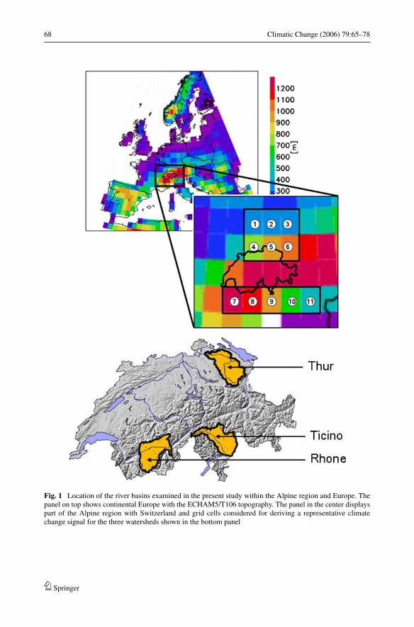
68 Climatic Change (2006) 79:65–78
Fig. 1 Location of the river basins examined in the present study within the Alpine region and Europe. Thepanel on top shows continental Europe with the ECHAM5/T106 topography. The panel in the center displayspart of the Alpine region with Switzerland and grid cells considered for deriving a representative climatechange signal for the three watersheds shown in the bottom panel
Springer
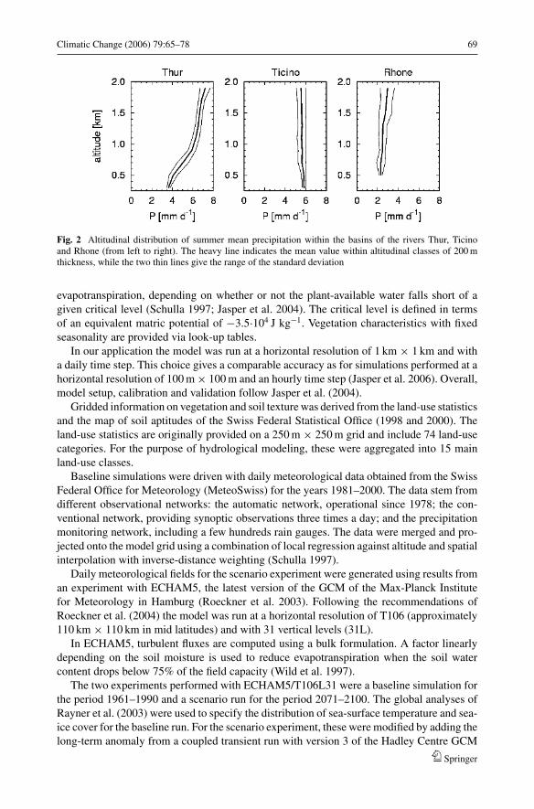
Climatic Change (2006) 79:65–78 69
Fig. 2 Altitudinal distribution of summer mean precipitation within the basins of the rivers Thur, Ticinoand Rhone (from left to right). The heavy line indicates the mean value within altitudinal classes of 200 mthickness, while the two thin lines give the range of the standard deviation
evapotranspiration, depending on whether or not the plant-available water falls short of agiven critical level (Schulla 1997; Jasper et al. 2004). The critical level is defined in termsof an equivalent matric potential of −3.5·104 J kg−1. Vegetation characteristics with fixedseasonality are provided via look-up tables.
In our application the model was run at a horizontal resolution of 1 km × 1 km and witha daily time step. This choice gives a comparable accuracy as for simulations performed at ahorizontal resolution of 100 m × 100 m and an hourly time step (Jasper et al. 2006). Overall,model setup, calibration and validation follow Jasper et al. (2004).
Gridded information on vegetation and soil texture was derived from the land-use statisticsand the map of soil aptitudes of the Swiss Federal Statistical Office (1998 and 2000). Theland-use statistics are originally provided on a 250 m × 250 m grid and include 74 land-usecategories. For the purpose of hydrological modeling, these were aggregated into 15 mainland-use classes.
Baseline simulations were driven with daily meteorological data obtained from the SwissFederal Office for Meteorology (MeteoSwiss) for the years 1981–2000. The data stem fromdifferent observational networks: the automatic network, operational since 1978; the con-ventional network, providing synoptic observations three times a day; and the precipitationmonitoring network, including a few hundreds rain gauges. The data were merged and pro-jected onto the model grid using a combination of local regression against altitude and spatialinterpolation with inverse-distance weighting (Schulla 1997).
Daily meteorological fields for the scenario experiment were generated using results froman experiment with ECHAM5, the latest version of the GCM of the Max-Planck Institutefor Meteorology in Hamburg (Roeckner et al. 2003). Following the recommendations ofRoeckner et al. (2004) the model was run at a horizontal resolution of T106 (approximately110 km × 110 km in mid latitudes) and with 31 vertical levels (31L).
In ECHAM5, turbulent fluxes are computed using a bulk formulation. A factor linearlydepending on the soil moisture is used to reduce evapotranspiration when the soil watercontent drops below 75% of the field capacity (Wild et al. 1997).
The two experiments performed with ECHAM5/T106L31 were a baseline simulation forthe period 1961–1990 and a scenario run for the period 2071–2100. The global analyses ofRayner et al. (2003) were used to specify the distribution of sea-surface temperature and sea-ice cover for the baseline run. For the scenario experiment, these were modified by adding thelong-term anomaly from a coupled transient run with version 3 of the Hadley Centre GCM
Springer
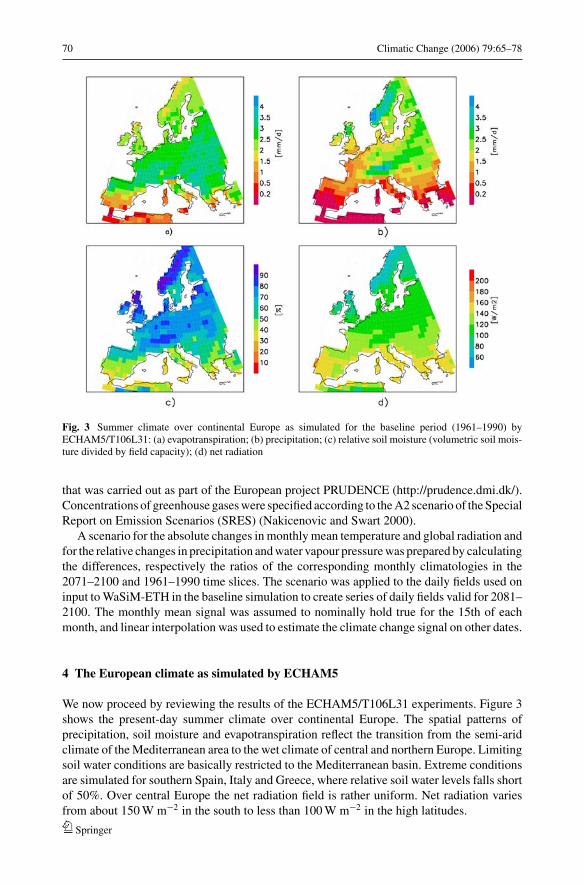
70 Climatic Change (2006) 79:65–78
Fig. 3 Summer climate over continental Europe as simulated for the baseline period (1961–1990) byECHAM5/T106L31: (a) evapotranspiration; (b) precipitation; (c) relative soil moisture (volumetric soil mois-ture divided by field capacity); (d) net radiation
that was carried out as part of the European project PRUDENCE (http://prudence.dmi.dk/).Concentrations of greenhouse gases were specified according to the A2 scenario of the SpecialReport on Emission Scenarios (SRES) (Nakicenovic and Swart 2000).
A scenario for the absolute changes in monthly mean temperature and global radiation andfor the relative changes in precipitation and water vapour pressure was prepared by calculatingthe differences, respectively the ratios of the corresponding monthly climatologies in the2071–2100 and 1961–1990 time slices. The scenario was applied to the daily fields used oninput to WaSiM-ETH in the baseline simulation to create series of daily fields valid for 2081–2100. The monthly mean signal was assumed to nominally hold true for the 15th of eachmonth, and linear interpolation was used to estimate the climate change signal on other dates.
4 The European climate as simulated by ECHAM5
We now proceed by reviewing the results of the ECHAM5/T106L31 experiments. Figure 3shows the present-day summer climate over continental Europe. The spatial patterns ofprecipitation, soil moisture and evapotranspiration reflect the transition from the semi-aridclimate of the Mediterranean area to the wet climate of central and northern Europe. Limitingsoil water conditions are basically restricted to the Mediterranean basin. Extreme conditionsare simulated for southern Spain, Italy and Greece, where relative soil water levels falls shortof 50%. Over central Europe the net radiation field is rather uniform. Net radiation variesfrom about 150 W m−2 in the south to less than 100 W m−2 in the high latitudes.
Springer
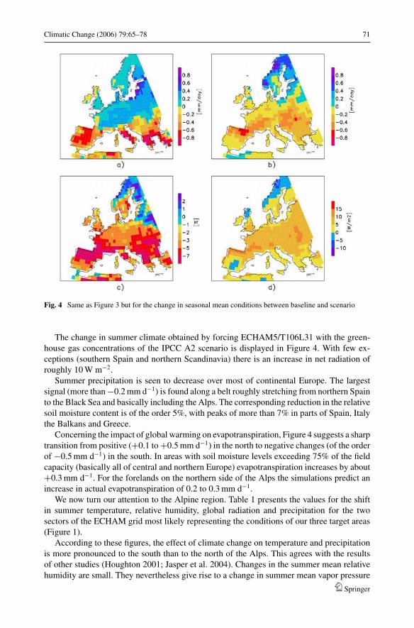
Climatic Change (2006) 79:65–78 71
Fig. 4 Same as Figure 3 but for the change in seasonal mean conditions between baseline and scenario
The change in summer climate obtained by forcing ECHAM5/T106L31 with the green-house gas concentrations of the IPCC A2 scenario is displayed in Figure 4. With few ex-ceptions (southern Spain and northern Scandinavia) there is an increase in net radiation ofroughly 10 W m−2.
Summer precipitation is seen to decrease over most of continental Europe. The largestsignal (more than −0.2 mm d−1) is found along a belt roughly stretching from northern Spainto the Black Sea and basically including the Alps. The corresponding reduction in the relativesoil moisture content is of the order 5%, with peaks of more than 7% in parts of Spain, Italythe Balkans and Greece.
Concerning the impact of global warming on evapotranspiration, Figure 4 suggests a sharptransition from positive (+0.1 to +0.5 mm d−1) in the north to negative changes (of the orderof −0.5 mm d−1) in the south. In areas with soil moisture levels exceeding 75% of the fieldcapacity (basically all of central and northern Europe) evapotranspiration increases by about+0.3 mm d−1. For the forelands on the northern side of the Alps the simulations predict anincrease in actual evapotranspiration of 0.2 to 0.3 mm d−1.
We now turn our attention to the Alpine region. Table 1 presents the values for the shiftin summer temperature, relative humidity, global radiation and precipitation for the twosectors of the ECHAM grid most likely representing the conditions of our three target areas(Figure 1).
According to these figures, the effect of climate change on temperature and precipitationis more pronounced to the south than to the north of the Alps. This agrees with the resultsof other studies (Houghton 2001; Jasper et al. 2004). Changes in the summer mean relativehumidity are small. They nevertheless give rise to a change in summer mean vapor pressure
Springer
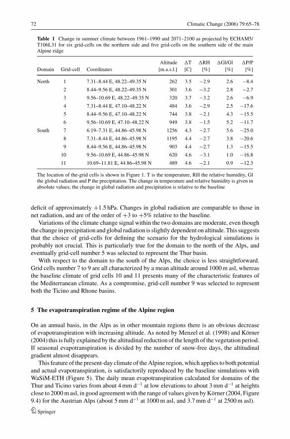
72 Climatic Change (2006) 79:65–78
Table 1 Change in summer climate between 1961–1990 and 2071–2100 as projected by ECHAM5/T106L31 for six grid-cells on the northern side and five grid-cells on the southern side of the mainAlpine ridge
Altitude �T �RH �Gl/Gl �P/PDomain Grid-cell Coordinates [m.a.s.l.] [C] [%] [%] [%]
North 1 7.31–8.44 E, 48.22–49.35 N 262 3.5 −2.9 2.6 −8.4
2 8.44–9.56 E, 48.22–49.35 N 301 3.6 −3.2 2.8 −2.7
3 9.56–10.69 E, 48.22–49.35 N 320 3.7 −3.2 2.6 −6.9
4 7.31–8.44 E, 47.10–48.22 N 484 3.6 −2.9 2.5 −17.6
5 8.44–9.56 E, 47.10–48.22 N 744 3.8 −2.1 4.3 −15.5
6 9.56–10.69 E, 47.10–48.22 N 949 3.8 −1.5 5.2 −11.7
South 7 6.19–7.31 E, 44.86–45.98 N 1256 4.3 −2.7 5.6 −25.0
8 7.31–8.44 E, 44.86–45.98 N 1195 4.4 −2.7 3.8 −20.6
9 8.44–9.56 E, 44.86–45.98 N 903 4.4 −2.7 1.3 −15.5
10 9.56–10.69 E, 44.86–45.98 N 620 4.6 −3.1 1.0 −16.8
11 10.69–11.81 E, 44.86–45.98 N 489 4.6 −2.1 0.9 −12.3
The location of the-grid cells is shown in Figure 1. T is the temperature, RH the relative humidity, Glthe global radiation and P the precipitation. The change in temperature and relative humidity is given inabsolute values; the change in global radiation and precipitation is relative to the baseline
deficit of approximately +1.5 hPa. Changes in global radiation are comparable to those innet radiation, and are of the order of +3 to +5% relative to the baseline.
Variations of the climate change signal within the two domains are moderate, even thoughthe change in precipitation and global radiation is slightly dependent on altitude. This suggeststhat the choice of grid-cells for defining the scenario for the hydrological simulations isprobably not crucial. This is particularly true for the domain to the north of the Alps, andeventually grid-cell number 5 was selected to represent the Thur basin.
With respect to the domain to the south of the Alps, the choice is less straightforward.Grid cells number 7 to 9 are all characterized by a mean altitude around 1000 m asl, whereasthe baseline climate of grid cells 10 and 11 presents many of the characteristic features ofthe Mediterranean climate. As a compromise, grid-cell number 9 was selected to representboth the Ticino and Rhone basins.
5 The evapotranspiration regime of the Alpine region
On an annual basis, in the Alps as in other mountain regions there is an obvious decreaseof evapotranspiration with increasing altitude. As noted by Menzel et al. (1998) and Korner(2004) this is fully explained by the altitudinal reduction of the length of the vegetation period.If seasonal evapotranspiration is divided by the number of snow-free days, the altitudinalgradient almost disappears.
This feature of the present-day climate of the Alpine region, which applies to both potentialand actual evapotranspiration, is satisfactorily reproduced by the baseline simulations withWaSiM-ETH (Figure 5). The daily mean evapotranspiration calculated for domains of theThur and Ticino varies from about 4 mm d−1 at low elevations to about 3 mm d−1 at heightsclose to 2000 m asl, in good agreement with the range of values given by Korner (2004, Figure9.4) for the Austrian Alps (about 5 mm d−1 at 1000 m asl, and 3.7 mm d−1 at 2500 m asl).
Springer
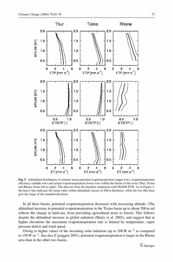
Climatic Change (2006) 79:65–78 73
Fig. 5 Altitudinal distribution of summer mean potential evapotranspiration (upper row), evapotranspirationefficiency (middle row) and actual evapotranspiration (lower row) within the basins of the rivers Thur, Ticinoand Rhone (from left to right). The data are from the baseline simulation with WaSiM-ETH. As in Figure 2,the heavy line indicates the mean value within altitudinal classes of 200 m thickness, while the two thin linesgive the range of the standard deviation
In all three basins, potential evapotranspiration decreases with increasing altitude. (Thealtitudinal increase in potential evapotranspiration in the Ticino basin up to about 500 m aslreflects the change in land-use, from prevailing agricultural areas to forest). This followsdespite the altitudinal increase in global radiation (Marty et al. 2002), and suggest that athigher elevations the maximum evapotranspiration rate is limited by temperature, vaporpressure deficit and wind speed.
Owing to higher values of the incoming solar radiation (up to 200 W m−2 as comparedto 150 W m−2. See also Z’graggen 2001), potential evapotranspiration is larger in the Rhonearea than in the other two basins.
Springer
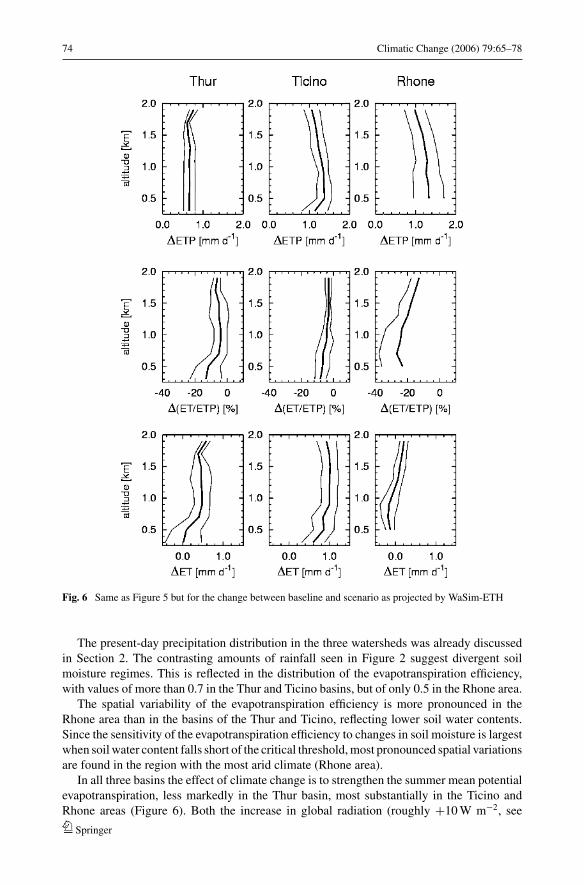
74 Climatic Change (2006) 79:65–78
Fig. 6 Same as Figure 5 but for the change between baseline and scenario as projected by WaSim-ETH
The present-day precipitation distribution in the three watersheds was already discussedin Section 2. The contrasting amounts of rainfall seen in Figure 2 suggest divergent soilmoisture regimes. This is reflected in the distribution of the evapotranspiration efficiency,with values of more than 0.7 in the Thur and Ticino basins, but of only 0.5 in the Rhone area.
The spatial variability of the evapotranspiration efficiency is more pronounced in theRhone area than in the basins of the Thur and Ticino, reflecting lower soil water contents.Since the sensitivity of the evapotranspiration efficiency to changes in soil moisture is largestwhen soil water content falls short of the critical threshold, most pronounced spatial variationsare found in the region with the most arid climate (Rhone area).
In all three basins the effect of climate change is to strengthen the summer mean potentialevapotranspiration, less markedly in the Thur basin, most substantially in the Ticino andRhone areas (Figure 6). Both the increase in global radiation (roughly +10 W m−2, see
Springer
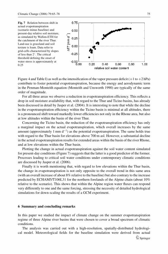
Climatic Change (2006) 79:65–78 75
Fig. 7 Relation between shift inactual evapotranspiration(scenario minus baseline) andpresent-day relative soil moisture,as simulated by WaSim-ETH forthe catchment of the river Thur.Land-use is grassland and soiltexture is loam. Data refer togrid-cells characterized by slopesof less than 2◦. The criticalthreshold defining the onset ofwater stress is approximately at0.25
Figure 4 and Table I) as well as the intensification of the vapor pressure deficit (+1 to +2 hPa)contribute to foster potential evapotranspiration, because the energy and aerodynamic termin the Penman-Monteith equation (Monteith and Unsworth 1990) are typically of the sameorder of magnitude.
For all three areas we observe a reduction in evapotranspiration efficiency. This reflects adrop in soil moisture availability that, with regard to the Thur and Ticino basins, has alreadybeen discussed in detail by Jasper et al. (2004). It is interesting to note that while the declinein the evapotranspiration efficiency within the Ticino basin is minimal at all altitudes, thereis a pronounced shift toward markedly lower efficiencies not only in the Rhone area, but alsoat low altitudes within the basin of the river Thur.
Concerning the Ticino basin, the reduction of the evapotranspiration efficiency has onlya marginal impact on the actual evapotranspiration, which overall increases by the sameamount (approximately 1 mm d−1) as the potential evapotranspiration. The same holds truewith regard to the Thur basin for elevations above 700 m asl. However, a substantial declinein the actual evapotranspiration results for extended areas within the basin of the river Rhone,and at low elevations within the Thur basin.
Plotting the change in actual evapotranspiration against the soil water content simulatedfor present-day conditions (Figure 7) suggests that the latter is a good predictor of the former.Processes leading to critical soil water conditions under contemporary climatic conditionsare discussed by Jasper et al. (2006).
Finally it is worth mentioning that, with regard to low elevations within the Thur basin,the change in evapotranspiration is not only opposite to the overall trend in this same area(with an overall increase of about 8% relative to the baseline) but also contrary to the increasepredicted by ECHAM5/T106L31 for the northern forelands of the Alpine chain (about 10%relative to the scenario). This shows that within the Alpine region water fluxes can respondvery differently to one and the same forcing, stressing the necessity of detailed hydrologicalsimulations for down-scaling the results of a GCM experiment.
6 Summary and concluding remarks
In this paper we studied the impact of climate change on the summer evapotranspirationregime of three Alpine river basins that were chosen to cover a broad spectrum of climaticconditions.
The analysis was carried out with a high-resolution, spatially-distributed hydrologi-cal model. Meteorological fields for the baseline simulation were derived from actual
Springer
76 Climatic Change (2006) 79:65–78
observations. Scenarios for the simulation of future climatic conditions where recoveredfrom the output of corresponding experiments carried out with ECHAM5/T106L31.
The simulations suggest that increased levels of solar radiation and reduced air humidityintensify the summer mean potential evapotranspiration. Changes in air humidity are pre-dicted in the order of 5% and, at first sight, appear to be unimportant. Nevertheless, theyaffect potential evapotranspiration in a consistent way. It is unfortunate that air humidity isoften neglected in scenarios utilized for impact studies; based on our experience, we rec-ommend that global radiation and air humidity be routinely included in regional climatescenarios.
While ECHAM predicts an increase in evapotranspiration over the entire Alpine region,the simulations with WaSiM-ETH indicate less uniform patterns of change, with an increasein the area to south of the Alps, but a decrease in the inner-Alpine domain and at low elevationsin the northern forelands. It has been pointed out by Jasper et al. (2006) that considerationof the spatial distribution of soil moisture as affected by slope, land-use and soil type isnecessary to understand this differential response to one and the same forcing. With respectto the Alpine region, a minimum spatial resolution of 1 km × 1 km or higher is required toadequately represent the dominant modes of spatial heterogeneity.
There is no doubt that the present results reflect the specific scenario used to force thehydrological model. In our study, the climate change signal was extracted from the results ofan experiment with ECHAM5/T106L31. Thanks to improved parameterizations (Roeckneret al. 2003) and enhanced vertical resolution (Roeckner et al. 2004), the impact of globalwarming on precipitation and soil moisture is less pronounced here than in studies based onprevious versions of ECHAM (Wild et al. 1996).
Overall, changes in summer mean climate as simulated by ECHAM5/T106L31 for theAlpine region are in line with those predicted by other GCMs (Houghton et al. 2001).However, the signal is stronger than found in regional climate scenarios derived by statisticaldownscaling from global fields (Jasper et al. 2004).
One has also to bear in mind that our scenario did not include changes in the inter-annualvariability of the Alpine climate. This is a crucial point, because in GCMs this variabilitydepends on the representation of the soil-atmosphere feedback (Schar et al. 2004). Whetherthis is simulated in a realistic way by ECHAM5 (as by other GCMs) remains to be verified.In general, a better representation of the hydrological cycle in GCMs is badly needed forquantifying the soil-atmosphere feedback in a more reliable way.
We also did not contemplate changes in the occurrence of extreme events. Understandingthe effect of climate change on the characteristics of extreme events (frequency and intensity)is fundamental for risk assessments. By looking at a variety of climate scenarios Fuhrer et al.(2006) arrived at the conclusion that the most remarkable trend in summer climate was adecrease in the frequency of wet days and shorter return times of heat waves. As shown byCalanca (2004), summer mean soil moisture levels are very sensitive with respect to changesin the frequency of wet days. Had we taken this into account in our analysis, we would havefound a more systematic and substantial decrease in actual evapotranspiration that suggestedby the present results.
Acknowledgements This work was carried out within the framework of the National Center of Competencein Research on Climate (NCCR Climate), an initiative funded by the Swiss National Science Foundation. Wethank Prof. H Wanner, Dr. M. Grosjean, Dr. E. Xoplaki and the whole staff for their commitment in supportof NCCR Climate. The Swiss Federal Office for Meteorology is kindly acknowledged for making its dataavailable. We also would like to thank two anonymous reviewers and Dr. Stefan Hagemann (Max-PlanckInstitute for Meteorology, Hamburg) for their critical but stimulating comments.
Springer
Climatic Change (2006) 79:65–78 77
References
Arnell N (1999) The effects of climate change on the hydrological regimes in Europe. Global Environ Change9:5–23
Behringer J, Buerki R, Fuhrer J (2000) Participatory integrated assessment of adaptation to climate change inAlpine tourism and mountain agriculture. Integr Assess 1:331–338
Beniston M (2003) Climatic change in mountain regions: A review of possible impacts. Climatic Change59:5–31
Beniston M, Keller F, Koffi B, Goyette S (2003) Estimates of snow accumulation and volume in the SwissAlps under changing climatic conditions. Theor Appl Clim 76:125–140
Beven KJ (2001) Rainfall-runoff modelling. The Primer. John Wiley and Sons, Chichester, p 360Brutsaert W, Parlange MB (1998) Hydrologic cycle explains the evaporation paradox. Nature 396:30Bugmann H (2003) Predicting the ecosystems effects of climate change. In: Canham CD, Cole JJ, Lauenroth
WK (eds) Models in ecosystem science, Princeton University Press, Princeton, pp 385–409Calanca P (2004) Interannual variability of summer mean soil moisture conditions in Switzerland dur-
ing the 20th century: A look using a stochastic soil moisture model. Water Resourc Res 40:W12502,doi:10.1029/2004WR003254
Carsel RF, Parrish RS (1988) Developing joint probability distributions of soil water retention characteristics.Water Resources Res 24(5):755–769
Doorenbos J, Kassam AH (1979) Yield Response to Water, FAO Irrigation and Drainage Paper 33, Food andAgriculture Organization of the United Nations, Rome, p 193.
Eagleson PS (2002) Ecohydrology. Darwinian expression of vegetation form and function. Cambridge Uni-versity Press, Cambridge, p 443
Feichter J, Roeckner E, Lohmann U, Liepert BG (2004) Nonlinear aspects of the climate response to greenhousegas and aerosol forcing. J. Climate 17:2384–2398
Fuhrer J, Beniston M, Fischlin A, Frei Ch, Goyette S, Jasper K, Pfister Ch (2006) Climate risks and theirimpact on agriculture and forests in Switzerland. Clim Change DOI: 10.1007/s10584-006-9106-6 (thisissue).
Golubev VS, Lawrimore JH, Groisman PY, Speranskaya NA, Zhuravin SA, Menne MJ, Peterson TC, MaloneRW (2001) Evaporation changes over the contiguous United States and the former USSR: A reassessment.Geophys Res Lett 28:2665–2668
Gurtz J, Baltensweiler A, Lang H (1999) Spatially distributed hydrotope-based modelling of evapotranspirationand runoff in mountainous basins. Hydrol Process 13:2751–2768
Gyalistras D, Schar C, Davies HC, Wanner H (1998) Future Alpine climate. In: Cebon P, Dahinden U, DaviesHC, Imboden D, Jager CG (eds) Views from the Alps: Regional perspectives on climate change. MITPress, Boston, pp 171–223
Houghton JT, Ding Y, Griggs DJ, Noguer M, van der Linden PJ, Dai X, Maskell K, Johnson CA (eds) (2001)Climate Change 2001, The Scientific Basis, Contribution of Working Group I to the Third AssessmentReport of the Intergovernmental Panel on Climate Change. Cambridge University Press, Cambridge, p 881.
Jasper K, Calanca P, Gyalistras D, Fuhrer J (2004) Differential impacts of climate change on the hydrologyof two Alpine river basins. Clim Res 26:113–129
Jasper K, Calanca P, Fuhrer J: (2006) Changes in summertime soil water patterns in complex terrain due toclimatic change. J Hydrology (in press)
Korner C (2004) Alpine plant life, 2nd edn. Springer, Berlin, and 4 colour plates, p 344Liepert BG, Feichter J, Lohmann U, Roeckner E (2004) Can aerosols spin down the water cycle in a warmer
and moister world? Geophys Res Lett 31:L06207, doi:10.1029/2003GL019060Marty C, Philipona R, Frohlich C, Ohmura A (2002) Altitude dependence of surface radiation fluxes and
cloud forcing in the Alps: Results from the Alpine surface radiation budget network. Theor Appl Climatol72:137–155
Menzel L, Lang H, Rohmann M (1998) Mean Annual Evapotranspiration 1973–1992, Hydrological Atlas ofSwitzerland, Plate 4.1, Federal Office of Topography, Bern
Monteith JL (1981) Climatic variation and the growth of crops. Quart J Roy Meteor Soc 107:749–774Monteith JL, Unsworth MH (1990) Principles of environmental physics, 2nd edn. Edward Arnold, London,
p 291Nakicenovic N, Swart R (eds) (2000) Emission Scenarios. Special Report of the Intergovernmental Panel on
Climate Change, Cambridge University Press, Cambridge, p 570Ohmura A, Wild M (2002) Is the hydrological cycle accelerating? Science 298:1345–1346Rayner NA, Parker DE, Horton EB, Folland CK, Alexander LV, Rowell DP, Kent EC, Kaplan A (2003) Global
analyses of sea surface temperature, sea ice, and night marine air temperature since the late nineteenthcentury. J Geophys Res 108(D14):4407, doi:10.1029/2002JD002670
Springer
78 Climatic Change (2006) 79:65–78
Riedo M, Gyalistras D, Fuhrer J (2000) Net primary production and carbon stocks in differently managedgrasslands: Simulation of site-specific sensitivity to an increase in atmospheric CO2 and to climatechange. Ecol Model 134:207–227
Riedo M, Gyalistras D, Fuhrer J (2001) Pasture response to elevated temperature and doubled CO2concentration: Assessing the spatial pattern across an alpine landscape. Clim Res. 17:19–31
Roderick ML, Farquhar GD (2002) The cause of decreased pan evaporation over the past 50 years. Science298:1410–1411
Roeckner E, Bengtsson L, Feichter J, Lelieveld J, Rodhe H (1999) Transient climate change simulations witha coupled atmosphere-ocean GCM including the tropospheric sulfur cycle. J Clim 12:3004–3032
Roeckner E, Bauml G, Bonaventura L, Brokopf R, Esch M, Giorgetta M, Hagemann S, Kirchner I, KornbluehL, Manzini E, Rhodin A, Schlese U, Schulzweida U, Tompkins A (2003) The Atmospheric GeneralCirculation Model ECHAM5. Part I: Model Description. Max Planck Institute for Meteorology, ReportNo. 349, Hamburg, p 127
Roeckner E, Brokopf R, Esch M, Giorgetta M, Hagemann S, Kornblueh, L, Manzini E, Schlese U,Schulzweida U (2004) The Atmospheric General Circulation Model ECHAM. Part II: Sensitivity ofSimulated Climate to Horizontal and Vertical Resolution. Max Planck Institute for Meteorology, ReportNo. 354, Hamburg, p 56
Schar C, Vidale DL, Luthi D, Frei C, Haberli C, Liniger MA, Appeazeller C (2004) The role of increasingtemperature variability in European summer heatwaves. Nature 427:332–336
Schulla J (1997) Hydrologische modellierung von Flussgebieten zur Abschatzung der Folgen vonKlimaanderungen, Zurcher Geographische Schriften, vol 69. Swiss Federal Institute of Technology,Zurich, p 161
Schulla J, Jasper K (2000) WaSiM-ETH: Model Description, Internal Report, Swiss Federal Institute ofTechnology, Zurich, p 166
Schwarb M, Frei C, Schar C, Daly C (2001a) Mean Annual Precipitation Throughout the European Alps1971–1990, Hydrological Atlas of Switzerland, Plate 2.6, Federal Office of Topography, Bern
Schwarb M, Frei C, Schar C, Daly C (2001b) Mean Seasonal Precipitation Throughout the European Alps1971–1990, Hydrological Atlas of Switzerland, Plate 2.7, Federal Office of Topography, Bern
Soil Conservation Service (1975) Soil taxonomy: A basic system of soil classification for making andinterpreting soil surveys. Agricultural Handbook no. 436, U.S. Department of Agriculture
Swiss Federal Statistical Office (1998) Arealstatistik 1992/1997. Neuchatel, SwitzerlandSwiss Federal Statistical Office (2000) Digital map of the soil aptitudes. Neuchatel, SwitzerlandTaylor HM, Jordan WR, Sinclair TR (eds) (1983) Limitations to efficient water use in crop production.
American Society of Agronomy, Crop Science Society of America, Soil Science Society of America,Madison, Wisconsin, p 538
Thornley JHM, Johnson IR (1990) Plant and crop modelling. Clarendon Press, Oxford, p 669Van Genuchten MT (1980) A closed-form equation for predicting the hydraulic conductivity of unsaturated
soils. Soil Sci Soc Am J 44:892–898Wild M, Dumenil L, Schulz JP (1996) Regional climate simulation with a high resolution GCM: Surface
hydrology. Climate Dynamics 12:755–774Wild M, Ohmura A, Cubasch U (1997) GCM simulated surface energy fluxes in climate change experiments.
J Climate 10:3093–3110Wild M, Ohmura A, Gilgen H (2004) On the consistency of trends in radiation and temperature records and
implications for the global hydrological cycle. Geophys Res Lett 31:L11201, doi:10.1029/2003GL019188Z’graggen L (2001) Strahlungsbilanz der Schweiz, Doctor of Natural Sciences Thesis Dissertation No.
14158, Swiss Federal Institute of Technology, Zurich, p 196
Springer
Climatic Change (2006) 79:79–102DOI 10.1007/s10584-006-9106-6
Climate risks and their impact on agriculture and forestsin Switzerland
J. Fuhrer · M. Beniston · A. Fischlin · Ch. Frei ·S. Goyette · K. Jasper · Ch. Pfister
Received: 14 September 2004 / Accepted: 1 March 2006 / Published online: 27 October 2006C© Springer Science + Business Media B.V. 2006
Abstract There is growing evidence that, as a result of global climate change, some of themost severe weather events could become more frequent in Europe over the next 50 to 100years. The paper aims to (i) describe observed trends and scenarios for summer heat waves,windstorms and heavy precipitation, based on results from simulations with global circulationmodels, regional climate models, and other downscaling procedures, and (ii) discuss potentialimpacts on agricultural systems and forests in Switzerland. Trends and scenarios projectmore frequent heavy precipitation during winter corresponding, for example, to a three-foldincrease in the exceedance of today’s 15-year extreme values by the end of the 21st century.This increases the risk of large-scale flooding and loss of topsoil due to erosion. In contrast,constraints in agricultural practice due to waterlogged soils may become less in a warmerclimate. In summer, the most remarkable trend is a decrease in the frequency of wet days,and shorter return times of heat waves and droughts. This increases the risk of losses of cropyield and forage quality. In forests, the more frequent occurrence of dry years may acceleratethe replacement of sensitive tree species and reduce carbon stocks, and the projected slightincrease in the frequency of extreme storms by the end of the century could increase the
J. Fuhrer (�) · K. JasperAgroscope FAL Reckenholz, Swiss Federal Research Station for Agroecology and Agriculture, AirPollution/Climate Group, Reckenholzstrasse 191, CH-8046 Zurich, Switzerlande-mail: [email protected]
M. Beniston · S. GoyetteDepartment of Geosciences, University of Fribourg, Fribourg, Switzerland
A. FischlinDepartment of Environmental Sciences, Institute of Terrestrial Ecology, Swiss Federal Institute ofTechnology ETHZ, Schlieren/Zurich, Switzerland
Ch. FreiDepartment of Environmental Sciences, Institute for Atmospheric and Climate Science, Swiss FederalInstitute of Technology ETHZ, Zurich, Switzerland
Ch. PfisterInstitute of History, University of Bern, Bern, Switzerland
Springer
80 Climatic Change (2006) 79:79–102
risk of windthrow. Some possible measures to maintain goods and services of agriculturaland forest ecosystems are mentioned, but it is suggested that more frequent extremes mayhave more severe consequences than progressive changes in means. In order to effectivelydecrease the risk for social and economic impacts, long-term adaptive strategies in agricultureand silviculture, investments for prevention, and new insurance concepts seem necessary.
Keywords Agriculture . Climate change . Extreme events . Forests . Society . Switzerland
1 Introduction
1.1 Scope and aim
Climate risks arise from complex interactions between climate, environment, social and eco-nomic systems, and they represent combinations of the likelihood of climate events and theirconsequences for society and the environment. Society can be affected either directly or indi-rectly. Recent examples of direct effects in Europe were the flood damage caused by extremerainfall in spring 1999 (Christensen and Christensen 2002), or the excess death particularly inFrance during the heat wave in 2003 (Valleron and Boumendil 2004). The present article dealswith potential indirect effects, which may occur via impacts on the provision of goods andservices to society by agricultural systems and forests. Historical events recorded in Switzer-land show that heavy precipitation and droughts were most important for agricultural crop andforage production (Pfister 1999). Typically, impacts of isolated events on croplands, i.e. yieldloss, were of short-term nature and could largely be alleviated by financial compensations.In the case of forests, winter storms are considered key climate risks, particularly in pre-alpine and alpine areas. Effects of climate extremes on forests can have both short-term andlong-term implications for standing biomass, tree health and species composition (Dale et al.2001; Bush et al. 2004), and similar principles apply to semi-natural grasslands (Grime et al.1994). A climate extreme can thus be considered an ecological disturbance in semi-naturalterrestrial ecosystems, and they are implicated as mechanistic drivers of species diversity, nu-trient cycling or carbon (C) stocks (Parmesan 2000). Consequently, the frequency of climateextremes is important with respect to the development and succession of ecosystems.
The types of extreme climatic events considered in this article have significant damagepotentials at the local and at the regional scales under today’s climate. But their importancecould increase over time, because extreme weather events may become more frequent aspart of global climate change (e.g., IPCC 2001). The link between climatic extremes andclimatic change is elusive because a few isolated events are difficult to relate in a statisticallymeaningful way to changes in mean climatic conditions (e.g., Frei and Schaer 2001; Benistonand Stephenson 2004).
The focus of this article is on climatological and ecological aspects. The aim is first toreview information from the Swiss research program NCCR ‘Climate’ (Swiss National Centerof Competence in Research ‘Climate’) and from other sources concerning temporal andspatial trends and scenarios for extremes in precipitation, temperature and wind, and secondlyto relate their current and projected occurrence to possible implications for agricultural landand forests in Switzerland.
1.2 Climatic extremes and their simulation
There are different possibilities to define ‘extreme events’. In a statistical sense, a climateextreme can be characterized by (1) the frequency of occurrence of anomalous weather (IPCC
Springer
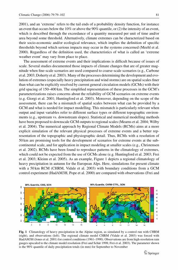
Climatic Change (2006) 79:79–102 81
2001), and an ‘extreme’ refers to the tail ends of a probability density function, for instancean event that occurs below the 10% or above the 90% quantile, or (2) the intensity of an event,which is described through the exceedance of a quantity measured per unit of time and/orarea beyond some threshold. Alternatively, climate extremes can be characterized based ontheir socio-economic and/or ecological relevance, which implies the definition of specificthresholds beyond which serious impacts may occur in the systems concerned (Meehl et al.2000). Regardless of the definition used, the characteristics of what is called an ‘extremeweather event’ may vary from place to place.
The assessment of extreme events and their implications is difficult because of issues ofscale. Several studies documented those impacts of climate changes that are of greater mag-nitude when fine-scale scenarios are used compared to coarse-scale scenarios (e.g., Carboneet al. 2003; Doherty et al. 2003). Many of the processes determining the development and evo-lution of extremes (especially heavy precipitation and wind storms) are on spatial scales finerthan what can be explicitly resolved by current general circulation models (GCMs) with theirgrid spacing of 150–400 km. The simplified representation of these processes in the GCM’sparameterizations raises concerns about the reliability of GCM scenarios on extreme events(e.g. Giorgi et al. 2001; Huntingford et al. 2003). Moreover, depending on the scope of theassessment, there can be a mismatch of spatial scales between what can be provided by aGCM and what is needed for impact modelling. This mismatch is particularly relevant whenoutput and input variables refer to different surface types or different topographic environ-ments (e.g., upstream vs. downstream slopes). Statistical and numerical modelling methodshave been proposed to downscale GCM outputs to regional scales (Mearns et al. 2004; Wilbyet al. 2004). The numerical approach by Regional Climate Models (RCMs) aims at a moreexplicit simulation of the relevant physical processes of extreme events and a better rep-resentation of the topographic and physiographic detail. Thus, RCMs with a resolution of50 km are promising tools for the development of scenarios for extreme events at the sub-continental scale, and for application in impact modeling at smaller scales (e.g., Christensenet al. 2002). RCMs have been found to reproduce patterns in the climatology of extremes,which could not be expected from the use of GCMs alone (e.g. Huntingford et al. 2003; Freiet al. 2003; Kleinn et al. 2005). As an example, Figure 1 depicts a regional climatology ofheavy precipitation in autumn for the European Alps. Here, simulations for present climatewith a 50 km RCM (CHRM, Vidale et al. 2003) with boundary conditions from a GCMcontrol experiment (HadAM3H, Pope et al. 2000) are compared with observations (Frei and
Fig. 1 Climatology of heavy precipitation in the Alpine region, as simulated by a control run with CHRM(right), and observations (left). The regional climate model CHRM (Vidale et al. 2003) was forced withHadAM3H (Jones et al. 2001) for control conditions (1961–1990). Observations are from high-resolution raingauges upscaled to the climate model resolution (Frei and Schar 1998; Frei et al. 2003). The parameter shownis the 90% quantile of daily precipitation totals (in mm) for September to November
Springer
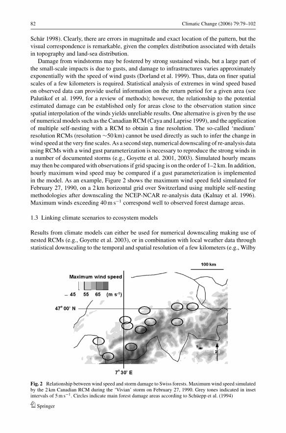
82 Climatic Change (2006) 79:79–102
Schar 1998). Clearly, there are errors in magnitude and exact location of the pattern, but thevisual correspondence is remarkable, given the complex distribution associated with detailsin topography and land-sea distribution.
Damage from windstorms may be fostered by strong sustained winds, but a large part ofthe small-scale impacts is due to gusts, and damage to infrastructures varies approximatelyexponentially with the speed of wind gusts (Dorland et al. 1999). Thus, data on finer spatialscales of a few kilometers is required. Statistical analysis of extremes in wind speed basedon observed data can provide useful information on the return period for a given area (seePalutikof et al. 1999, for a review of methods); however, the relationship to the potentialestimated damage can be established only for areas close to the observation station sincespatial interpolation of the winds yields unreliable results. One alternative is given by the useof numerical models such as the Canadian RCM (Caya and Laprise 1999), and the applicationof multiple self-nesting with a RCM to obtain a fine resolution. The so-called ‘medium’resolution RCMs (resolution ∼50 km) cannot be used directly as such to infer the change inwind speed at the very fine scales. As a second step, numerical downscaling of re-analysis datausing RCMs with a wind gust parameterization is necessary to reproduce the strong winds ina number of documented storms (e.g., Goyette et al. 2001, 2003). Simulated hourly meansmay then be compared with observations if grid spacing is on the order of 1–2 km. In addition,hourly maximum wind speed may be compared if a gust parameterization is implementedin the model. As an example, Figure 2 shows the maximum wind speed field simulated forFebruary 27, 1990, on a 2 km horizontal grid over Switzerland using multiple self-nestingmethodologies after downscaling the NCEP-NCAR re-analysis data (Kalnay et al. 1996).Maximum winds exceeding 40 m s−1 correspond well to observed forest damage areas.
1.3 Linking climate scenarios to ecosystem models
Results from climate models can either be used for numerical downscaling making use ofnested RCMs (e.g., Goyette et al. 2003), or in combination with local weather data throughstatistical downscaling to the temporal and spatial resolution of a few kilometers (e.g., Wilby
Fig. 2 Relationship between wind speed and storm damage to Swiss forests. Maximum wind speed simulatedby the 2 km Canadian RCM during the ‘Vivian’ storm on February 27, 1990. Grey tones indicated in insetintervals of 5 m s−1. Circles indicate main forest damage areas according to Schuepp et al. (1994)
Springer
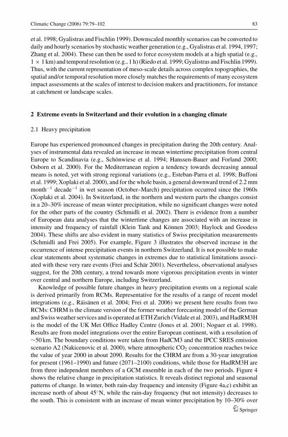
Climatic Change (2006) 79:79–102 83
et al. 1998; Gyalistras and Fischlin 1999). Downscaled monthly scenarios can be converted todaily and hourly scenarios by stochastic weather generation (e.g., Gyalistras et al. 1994, 1997;Zhang et al. 2004). These can then be used to force ecosystem models at a high spatial (e.g.,1 × 1 km) and temporal resolution (e.g., 1 h) (Riedo et al. 1999; Gyalistras and Fischlin 1999).Thus, with the current representation of meso-scale details across complex topographies, thespatial and/or temporal resolution more closely matches the requirements of many ecosystemimpact assessments at the scales of interest to decision makers and practitioners, for instanceat catchment or landscape scales.
2 Extreme events in Switzerland and their evolution in a changing climate
2.1 Heavy precipitation
Europe has experienced pronounced changes in precipitation during the 20th century. Anal-yses of instrumental data revealed an increase in mean wintertime precipitation from centralEurope to Scandinavia (e.g., Schonwiese et al. 1994; Hanssen-Bauer and Forland 2000;Osborn et al. 2000). For the Mediterranean region a tendency towards decreasing annualmeans is noted, yet with strong regional variations (e.g., Esteban-Parra et al. 1998; Buffoniet al. 1999; Xoplaki et al. 2000), and for the whole basin, a general downward trend of 2.2 mmmonth−1 decade−1 in wet season (October–March) precipitation occurred since the 1960s(Xoplaki et al. 2004). In Switzerland, in the northern and western parts the changes consistin a 20–30% increase of mean winter precipitation, while no significant changes were notedfor the other parts of the country (Schmidli et al. 2002). There is evidence from a numberof European data analyses that the wintertime changes are associated with an increase inintensity and frequency of rainfall (Klein Tank and Konnen 2003; Haylock and Goodess2004). These shifts are also evident in many statistics of Swiss precipitation measurements(Schmidli and Frei 2005). For example, Figure 3 illustrates the observed increase in theoccurrence of intense precipitation events in northern Switzerland. It is not possible to makeclear statements about systematic changes in extremes due to statistical limitations associ-ated with these very rare events (Frei and Schar 2001). Nevertheless, observational analysessuggest, for the 20th century, a trend towards more vigorous precipitation events in winterover central and northern Europe, including Switzerland.
Knowledge of possible future changes in heavy precipitation events on a regional scaleis derived primarily from RCMs. Representative for the results of a range of recent modelintegrations (e.g., Raisanen et al. 2004; Frei et al. 2006) we present here results from twoRCMs: CHRM is the climate version of the former weather forecasting model of the Germanand Swiss weather services and is operated at ETH Zurich (Vidale et al. 2003), and HadRM3His the model of the UK Met Office Hadley Centre (Jones et al. 2001; Noguer et al. 1998).Results are from model integrations over the entire European continent, with a resolution of∼50 km. The boundary conditions were taken from HadCM3 and the IPCC SRES emissionscenario A2 (Nakicenovic et al. 2000), where atmospheric CO2 concentration reaches twicethe value of year 2000 in about 2090. Results for the CHRM are from a 30-year integrationfor present (1961–1990) and future (2071–2100) conditions, while those for HadRM3H arefrom three independent members of a GCM ensemble in each of the two periods. Figure 4shows the relative change in precipitation statistics. It reveals distinct regional and seasonalpatterns of change. In winter, both rain-day frequency and intensity (Figure 4a,c) exhibit anincrease north of about 45◦N, while the rain-day frequency (but not intensity) decreases tothe south. This is consistent with an increase of mean winter precipitation by 10–30% over
Springer
84 Climatic Change (2006) 79:79–102
1900 1920 1940 1960 1980 2000
0
8
6
4
2
stnevE fo #
Fig. 3 Evolution of the number of heavy precipitation events per winter in northern Switzerland (days, whenthe daily total exceeds the climatological 90% quantile). Blue shaded: inter-quartile range from 35 stations;bold black line: smoothed time series (smoothing window is 11 years); red line: long-term trend estimatedfrom the pooled data using logistic regression. The trend corresponds to an increase by 75% over the 20thcentury and is statistically significant at the 5% level (Schmidli and Frei 2005). (Courtesy of J. Schmidli, ETHZurich)
most of central and northern Europe, and a decrease over the Mediterranean (not shown).These changes are reflected in changes for intense and heavy precipitation. For example, the90% quantile, i.e. the typical rainfall with a recurrence of 20–30 days, increases by about20% over northern Europe in winter.
An analysis for extreme events based on the method of extreme value statistics (see Freiet al. 2006 for details) was undertaken for the HadRM3H integration and is displayed inFigure 5. For winter, the HadRM3H model reveals an increase in the 5-year maximum 5-dayprecipitation event by 10–30% over large areas of central and northern Europe, includingSwitzerland (Figure 5a). This change corresponds roughly to a three-fold increase in fre-quency, i.e. the 15-year event of today’s climate would become a 5-year event.
In summer, the most remarkable change is a strong decrease in the frequency of wetdays (Figure 5b), for instance to about half in the Mediterranean, which goes along with a20–50% decrease of mean summer precipitation (not shown). There is no similar tendencyof drying in rainfall intensity. For example, a central part of Europe including Switzerland,which undergoes significant drying in the mean, shows a slight increase in the 90% quantile(Figure 4f) and the 5-year return period of extreme rainfall (Figure 5b). Yet the changes forextremes are at the border of statistical significance.
The results from the selected model integrations are very similar to results found in otherRCM experiments (e.g., Durman et al. 2001; Christensen and Christensen 2003; Raisanenet al. 2004; Frei et al. 2006) in terms of their seasonal distribution and their larger-scalegeographic pattern. However, the magnitude of change and the smaller-scale pattern varyconsiderably between RCMs. Hence, although a general increase of heavy precipitation dur-ing wintertime is noted in the simulations for the territory of Switzerland, there remainsconsiderable uncertainty about the magnitude of this increase, even under a prescribed emis-sion scenario. Moreover, little can be said today about regional differences within the country.Particularly uncertain are current scenarios of heavy precipitation for the summer season,where results for Central Europe vary even in the sign between different models (Raisanenet al. 2004; Frei et al. 2006). However, it is interesting to see the similarity among manymodels: the frequency of extreme precipitation events decreases modestly, or even increases,
Springer
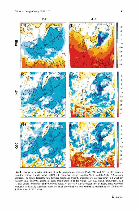
Climatic Change (2006) 79:79–102 85
Fig. 4 Change in selected statistics of daily precipitation between 1961–1990 and 2071–2100. Scenariofrom the regional climate model CHRM with boundary forcing from HadAM3H and the SRES A2 emissionscenario. The panels depict the ratio between future and present climate for wet-day frequency (a, b), wet-dayintensity (c, d) and 90% quantile of daily precipitation (e, f), for winter (DJF, a, c, e) and summer (JJA, b, d,f). Blue colors for increase and yellow/red colors for decrease. Thick contour lines delineate areas where thechange is statistically significant at the 5% level, according to a non-parametric resampling test (Courtesy ofS. Fukutome, ETH Zurich)
Springer
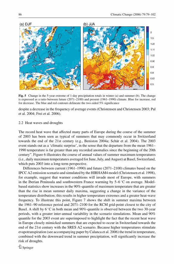
86 Climatic Change (2006) 79:79–102
Fig. 5 Change in the 5-year extreme of 1-day precipitation totals in winter (a) and summer (b). The changeis expressed as a ratio between future (2071–2100) and present (1961–1990) climate. Blue for increase, redfor decrease. The blue and red contours delineate the two-sided 5% significance
despite a decrease in the frequency of average events (Christensen and Christensen 2003; Palet al. 2004; Frei et al. 2006).
2.2 Heat waves and droughts
The record heat wave that affected many parts of Europe during the course of the summerof 2003 has been seen as typical of summers that may commonly occur in Switzerlandtowards the end of the 21st century (e.g., Beniston 2004a; Schar et al. 2004). The 2003event stands out as a ‘climatic surprise’, in the sense that the departure from the mean 1961–1990 temperature is far greater than any recorded anomalies since the beginning of the 20thcentury”. Figure 6 illustrates the course of annual values of summer maximum temperatures(i.e., daily maximum temperatures averaged for June, July, and August) at Basel, Switzerland,which puts 2003 into a long-term perspective.
Differences between current (1961–1990) and future (2071–2100) climates based on theIPCC A2 emission scenario and simulated by the HIRHAM4 model (Christensen et al. 1998),for example, suggest that warmer conditions will invade most of Europe, with summersin the Iberian Peninsula and southwestern France warming by 5–6 ◦C on average. Model-based statistics show increases in the 90%-quantile of maximum temperature that are greaterthan the rise in mean summer daily maxima, suggesting a change in the variance of thetemperature distribution; this results in higher temperature extremes and a greater heat-wavefrequency. To illustrate this point, Figure 7 shows the shift in summer maxima betweenthe 1961–90 reference period and 2071–2100 for the RCM grid-point closest to the city ofBasel. A shift by 6 ◦C in both mean and 90%-quantile is observed between the two 30-yearperiods, with a greater inter-annual variability in the scenario simulations. Mean and 90%quantile for the 2003 event are superimposed to highlight the fact that the recent heat wavein Europe closely mimicked summers that are expected to occur in Switzerland towards theend of the 21st century with the SRES A2 scenario. Because higher temperatures stimulateevapotranspiration (see accompanying paper by Calanca et al. 2006) the trend in temperature,combined with the downward trend in summer precipitation, will significantly increase therisk of droughts.
Springer
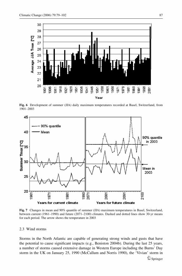
Climatic Change (2006) 79:79–102 87
Fig. 6 Development of summer (JJA) daily maximum temperatures recorded at Basel, Switzerland, from1901–2003
Fig. 7 Changes in mean and 90% quantile of summer (JJA) maximum temperatures in Basel, Switzerland,between current (1961–1990) and future (2071–2100) climates. Dashed and dotted lines show 30-yr meansfor each period. The arrow shows the temperature in 2003
2.3 Wind storms
Storms in the North Atlantic are capable of generating strong winds and gusts that havethe potential to cause significant impacts (e.g., Beniston 2004b). During the last 25 years,a number of storms caused extensive damage in Western Europe including the Burns’ Daystorm in the UK on January 25, 1990 (McCallum and Norris 1990), the ‘Vivian’ storm in
Springer
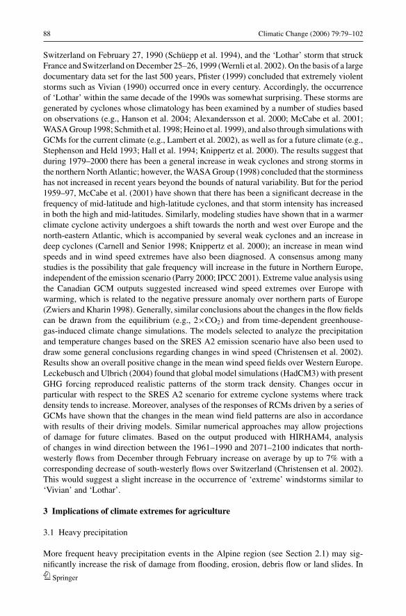
88 Climatic Change (2006) 79:79–102
Switzerland on February 27, 1990 (Schuepp et al. 1994), and the ‘Lothar’ storm that struckFrance and Switzerland on December 25–26, 1999 (Wernli et al. 2002). On the basis of a largedocumentary data set for the last 500 years, Pfister (1999) concluded that extremely violentstorms such as Vivian (1990) occurred once in every century. Accordingly, the occurrenceof ‘Lothar’ within the same decade of the 1990s was somewhat surprising. These storms aregenerated by cyclones whose climatology has been examined by a number of studies basedon observations (e.g., Hanson et al. 2004; Alexandersson et al. 2000; McCabe et al. 2001;WASA Group 1998; Schmith et al. 1998; Heino et al. 1999), and also through simulations withGCMs for the current climate (e.g., Lambert et al. 2002), as well as for a future climate (e.g.,Stephenson and Held 1993; Hall et al. 1994; Knippertz et al. 2000). The results suggest thatduring 1979–2000 there has been a general increase in weak cyclones and strong storms inthe northern North Atlantic; however, the WASA Group (1998) concluded that the storminesshas not increased in recent years beyond the bounds of natural variability. But for the period1959–97, McCabe et al. (2001) have shown that there has been a significant decrease in thefrequency of mid-latitude and high-latitude cyclones, and that storm intensity has increasedin both the high and mid-latitudes. Similarly, modeling studies have shown that in a warmerclimate cyclone activity undergoes a shift towards the north and west over Europe and thenorth-eastern Atlantic, which is accompanied by several weak cyclones and an increase indeep cyclones (Carnell and Senior 1998; Knippertz et al. 2000); an increase in mean windspeeds and in wind speed extremes have also been diagnosed. A consensus among manystudies is the possibility that gale frequency will increase in the future in Northern Europe,independent of the emission scenario (Parry 2000; IPCC 2001). Extreme value analysis usingthe Canadian GCM outputs suggested increased wind speed extremes over Europe withwarming, which is related to the negative pressure anomaly over northern parts of Europe(Zwiers and Kharin 1998). Generally, similar conclusions about the changes in the flow fieldscan be drawn from the equilibrium (e.g., 2×CO2) and from time-dependent greenhouse-gas-induced climate change simulations. The models selected to analyze the precipitationand temperature changes based on the SRES A2 emission scenario have also been used todraw some general conclusions regarding changes in wind speed (Christensen et al. 2002).Results show an overall positive change in the mean wind speed fields over Western Europe.Leckebusch and Ulbrich (2004) found that global model simulations (HadCM3) with presentGHG forcing reproduced realistic patterns of the storm track density. Changes occur inparticular with respect to the SRES A2 scenario for extreme cyclone systems where trackdensity tends to increase. Moreover, analyses of the responses of RCMs driven by a series ofGCMs have shown that the changes in the mean wind field patterns are also in accordancewith results of their driving models. Similar numerical approaches may allow projectionsof damage for future climates. Based on the output produced with HIRHAM4, analysisof changes in wind direction between the 1961–1990 and 2071–2100 indicates that north-westerly flows from December through February increase on average by up to 7% with acorresponding decrease of south-westerly flows over Switzerland (Christensen et al. 2002).This would suggest a slight increase in the occurrence of ‘extreme’ windstorms similar to‘Vivian’ and ‘Lothar’.
3 Implications of climate extremes for agriculture
3.1 Heavy precipitation
More frequent heavy precipitation events in the Alpine region (see Section 2.1) may sig-nificantly increase the risk of damage from flooding, erosion, debris flow or land slides. In
Springer
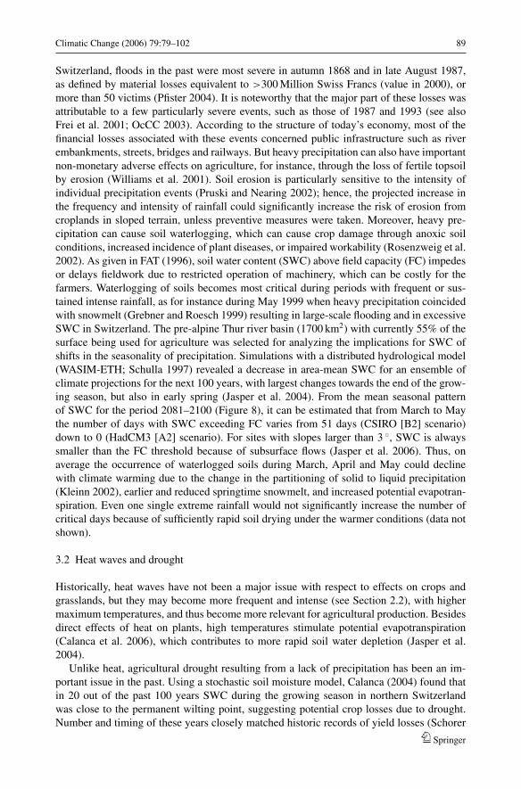
Climatic Change (2006) 79:79–102 89
Switzerland, floods in the past were most severe in autumn 1868 and in late August 1987,as defined by material losses equivalent to >300 Million Swiss Francs (value in 2000), ormore than 50 victims (Pfister 2004). It is noteworthy that the major part of these losses wasattributable to a few particularly severe events, such as those of 1987 and 1993 (see alsoFrei et al. 2001; OcCC 2003). According to the structure of today’s economy, most of thefinancial losses associated with these events concerned public infrastructure such as riverembankments, streets, bridges and railways. But heavy precipitation can also have importantnon-monetary adverse effects on agriculture, for instance, through the loss of fertile topsoilby erosion (Williams et al. 2001). Soil erosion is particularly sensitive to the intensity ofindividual precipitation events (Pruski and Nearing 2002); hence, the projected increase inthe frequency and intensity of rainfall could significantly increase the risk of erosion fromcroplands in sloped terrain, unless preventive measures were taken. Moreover, heavy pre-cipitation can cause soil waterlogging, which can cause crop damage through anoxic soilconditions, increased incidence of plant diseases, or impaired workability (Rosenzweig et al.2002). As given in FAT (1996), soil water content (SWC) above field capacity (FC) impedesor delays fieldwork due to restricted operation of machinery, which can be costly for thefarmers. Waterlogging of soils becomes most critical during periods with frequent or sus-tained intense rainfall, as for instance during May 1999 when heavy precipitation coincidedwith snowmelt (Grebner and Roesch 1999) resulting in large-scale flooding and in excessiveSWC in Switzerland. The pre-alpine Thur river basin (1700 km2) with currently 55% of thesurface being used for agriculture was selected for analyzing the implications for SWC ofshifts in the seasonality of precipitation. Simulations with a distributed hydrological model(WASIM-ETH; Schulla 1997) revealed a decrease in area-mean SWC for an ensemble ofclimate projections for the next 100 years, with largest changes towards the end of the grow-ing season, but also in early spring (Jasper et al. 2004). From the mean seasonal patternof SWC for the period 2081–2100 (Figure 8), it can be estimated that from March to Maythe number of days with SWC exceeding FC varies from 51 days (CSIRO [B2] scenario)down to 0 (HadCM3 [A2] scenario). For sites with slopes larger than 3 ◦, SWC is alwayssmaller than the FC threshold because of subsurface flows (Jasper et al. 2006). Thus, onaverage the occurrence of waterlogged soils during March, April and May could declinewith climate warming due to the change in the partitioning of solid to liquid precipitation(Kleinn 2002), earlier and reduced springtime snowmelt, and increased potential evapotran-spiration. Even one single extreme rainfall would not significantly increase the number ofcritical days because of sufficiently rapid soil drying under the warmer conditions (data notshown).
3.2 Heat waves and drought
Historically, heat waves have not been a major issue with respect to effects on crops andgrasslands, but they may become more frequent and intense (see Section 2.2), with highermaximum temperatures, and thus become more relevant for agricultural production. Besidesdirect effects of heat on plants, high temperatures stimulate potential evapotranspiration(Calanca et al. 2006), which contributes to more rapid soil water depletion (Jasper et al.2004).
Unlike heat, agricultural drought resulting from a lack of precipitation has been an im-portant issue in the past. Using a stochastic soil moisture model, Calanca (2004) found thatin 20 out of the past 100 years SWC during the growing season in northern Switzerlandwas close to the permanent wilting point, suggesting potential crop losses due to drought.Number and timing of these years closely matched historic records of yield losses (Schorer
Springer
90 Climatic Change (2006) 79:79–102
Fig. 8 Seasonal pattern of mean daily volumetric soil water content (SWC) for farmland on loamy soils andgentle slopes (<3 ◦) in the Swiss Thur basin simulated with the runoff and water balance model WaSiM-ETH(e.g., Schulla 1997; Jasper et al. 2006). Data are results of the control run (1981–2000) and the 2081–2100projections obtained by using two different climate scenarios (HadCM3 (A2) and CSIRO (B2) (see Jasperet al. 2006). Inset: Projected changes in mean monthly precipitation (P)
1992; Pfister 1999). Drought in 1947 had the most devastating effect on Swiss agriculturebecause of its long duration (July to October) and its large geographical extent. Wheat yieldsin northwestern and central Europe dropped by 25–35% relative to the long-term average,and fodder became scarce and expensive throughout the continent (FAO data, cited in Schorer1992). In contrast to the droughts in 1952 and 1953, import of forage into Switzerland waslimited because of the concurrent crop losses in neighboring European countries (Schorer1992). More recently, in 2003 yields of various crops and fodder cereals decreased by anaverage of 20% relative to the mean for 1991–99 (Keller and Fuhrer 2004). Low forageproduction during the second half of the season resulted in a shortage of fodder, which wascompensated by increased imports at a reduced tax. Overall, the extreme weather in 2003lowered the national net revenue of farmers from plant production by 11.1%, equivalent toabout 500 Million Swiss Francs, while the fluctuations in supply had no effect on final pricesof agricultural goods (Swiss Federal Office for Agriculture 2003). Hence, an isolated extremeevent may not have lasting economic consequences.
To estimate future risks due to low SWC, Jasper et al. (2004) estimated for both northernand southern Switzerland an increase in average annual ET by 9–23% by 2071–2100, relativeto 1981–2000, with largest changes during the summer months (see also Calanca et al. 2006).Combined with the projected reduction in summer precipitation (Schmidli and Frei 2005),this trend increases the likelihood of episodic drought. This is supported by preliminaryestimates of the probability of the occurrence of agricultural drought on the Swiss CentralPlateau from currently about 10–15% to over 50% towards the end of the century (Calanca2006).
Effects of more frequent drought concern not only croplands, but also permanent grass-lands, which in Switzerland cover around 75% of the agricultural land and sustain domesticmeat and dairy production. The value associated with animal production was estimated at5.2 billion Swiss Francs, or 68% of the total value of agricultural production (Swiss Farm-ers’ Union 2001). Using a simple grassland model, Calanca and Fuhrer (2005) showed thatgrassland productivity could benefit in the future from moderately increased temperatures,
Springer
Climatic Change (2006) 79:79–102 91
higher radiation, and elevated CO2. But if changes in the thermal and hydrological con-ditions were more pronounced and similar to the conditions in 2003, grassland productioncould become strongly water-limited. The authors estimated that the costs for setting up fixedirrigation systems for the entire grassland area of Switzerland would amount to 0.3 billionSwiss Francs annually, which is substantial but still a reasonable amount when compared tothe present value of grassland production. Alternatively, fodder imports would be necessaryfrom regions with more favorable conditions.
Effects of drought include not only decreased productivity, but also declining qualityresulting from the formation of gaps in the sward, which can be colonized by weeds (cf.Luscher et al. 2005); in turn, this has negative implications for animal nutrition. While inmanaged systems this effect can be addressed by farmers’ interventions such as re-seeding,in semi-natural grasslands with little or no influence of management natural re-colonizationfollowing perturbation by drought is considered a primary driver of vegetation dynamics.A study by Stampfli and Zeiter (2004) in southern Switzerland (Ticino) confirmed thatmore frequent droughts might drive grassland vegetation changes with local colonizationand extinction, as suggested earlier by Grime et al. (1994). Hence, increased frequency ofdrought has important economic effects in productive grassland systems and ecologicallyrelevant effects in semi-natural systems.
4 Implications of climate extremes for forests
4.1 Wind storms
Storm is considered the most important natural disturbance agent in European forests. It isresponsible for one third of total unplanned fellings (Brassel and Brandli 1999). Since 1868European forests were impacted at least 16 times by the effects of several severe storms(Schelhaas et al. 2003), and 10 times since the early 1950s with windthrow of over 20 millionm3; damages in 1990 and 1999 were by far the worst of all these years (UN/ECE TimberCommittee 2000). Apparently, windthrow damage in Europe has increased in the past century;yet, loss of timber was typically smaller than annual timber harvests (Schelhaas et al. 2003).An exception was storm ‘Lothar’ in 1999, which was among the four most extreme eventssince 1500 (Pfister 1999) and threw 12.7 × 10⁶ m3 in Switzerland, which is equivalent to 2.8times the average annual timber harvest (e.g. Dobbertin et al. 2002). Wind velocities on topof the Jura Mountains near Geneva exceeded 200 km h−1, and in other areas of Switzerlandwinds were measured at 240 km h−1. The total amount of damage was estimated at more than750 million Swiss Francs, plus another 38 million due to damages to individual trees and fruittrees (WSL/BUWAL 1999). Because of the large spatial extent, the abundance of windthrowntimber affected the European market: roundwood markets were temporarily in chaos afterthe ‘Lothar’ event, with sharply falling prices (UN/ECE Timber Committee 2000). Similarto the effects of storms in 1990 on markets for wood products, fluctuations in supply andprice were absorbed during primary processing and there were little distinguishable effectsin prices or sales for sawn wood, panels and pulp. Greater market calamity was mitigatedthrough sector solidarity.
Besides the loss of timber, windthrow can also have positive ecological effects(Schonenberger 2001), but where damage levels exceed harvesting or salvage harvestingcosts are high, e.g. in mountainous terrain, adverse effects of wind storms outweigh anypositive ones resulting from wood utilization (Widmer et al. 2004). As it dries, the wind-blown wood presents ideal conditions for massive fires and insect outbreaks, thus threatening
Springer
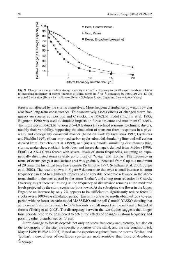
92 Climatic Change (2006) 79:79–102
5 10 15 20
10
20
30
40
50
60
70
80
90
100
Storm frequency (number ha-1 yr-1)
Rel
ativ
e ch
ange
in C
sto
rage
cap
acity
(%
)
Bern, Central Plateau
Sion, Valais
Bever, Engadine (pre-alpine)
Fig. 9 Change in average carbon storage capacity (t C ha−1) of young to middle-aged stands in relationto increasing frequency of storms (number of storm events ha−1 yr−1) simulated by FORCLIM 2.6–4.0 forselected Swiss sites (Bern - Swiss Plateau, Bever - Subalpine Upper Engadine, Sion – Rhone Valley)
forests not affected by the storms themselves. More frequent disturbance by windthrow canalso have long-term consequences. To quantitatively assess effects of changed storm fre-quency on species composition and C stocks, the FORCLIM model (Fischlin et al. 1995;Bugmann 1996) was used to simulate impacts on forest structure and maximum C-stocks.The most recent FORCLIM version 2.6–4.0 features (i) a refined response to climatic drivers,notably their variability, supporting the simulation of transient forest responses in a phys-ically and ecologically consistent manner (based on work by Gyalistras 1997; Gyalistrasand Fischlin 1999), (ii) an improved carbon cycle submodel simulating litter and soil carbonderived from Perruchoud et al. (1999), and (iii) a submodel simulating disturbances (fire,storms, avalanches, rockfall, landslides, and insect damage), derived from Mader (1999).FORCLIM 2.6–4.0 was forced with several levels of storm frequencies, assuming an expo-nentially distributed storm severity up to those of ‘Vivian’ and ‘Lothar’. The frequency interms of events per year and surface area was gradually increased from 0 up to a maximumof 20 times the historical base line estimate (Schmidtke 1997; Schelhaas et al. 2003; Jungoet al. 2002). The results shown in Figure 9 demonstrate that even a small increase in stormfrequency can lead to significant impacts of considerable economic relevance in the short-term, similar to the ones caused by the storm ‘Lothar’, and a long-term reduction in C stock.Diversity might increase, as long as the frequency of disturbance remains at the moderatelevels projected by the storm scenarios (not shown). At the sub-alpine site Bever in the UpperEngadine an increase by only 7% appears to be sufficient to significantly reduce forest Cstocks over a 1000-year simulation period. This is in contrast to results obtained for a 40-yearperiod with the forest scenario model MASSIMO and the soil C model YASSO showing thatan increase in storm frequency by 30% has only a small impact on the national C budget offorests (Thurig et al. 2005). The discrepancy between the two studies suggests that longertime periods need to be considered to detect the effects of changes in storm frequency andpossibly other disturbances on forests.
Storm damage to forests depends not only on storm frequency and intensity, but also onthe topography of the site, the specific properties of the stand, and the site conditions (cf.Mayer 1989; BUWAL 2005). Based on the experience gained from the storms ‘Vivian’ and‘Lothar’, monocultures of coniferous species are more sensitive than those of deciduous
Springer
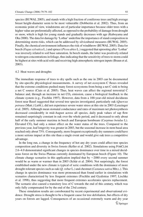
Climatic Change (2006) 79:79–102 93
species (BUWAL 2005), and stands with a high fraction of coniferous trees and high averagebreast height-diameter seem to be most vulnerable (Dobbertin et al. 2002). Thus, from aneconomic point of view, windstorms are of particular importance because older trees with ahigher value are preferentially affected, as opposed to the probability of damage from droughtor snow, which is high for young stands and gradually decreases with age (Kuboyama andOka 2000). The data for damage by ‘Lothar’ underline the importance of stand composition indetermining storm risks, which can be addressed by silvicultural measures (BUWAL 2005).Finally, the chemical environment influences the risk of windthrow (BUWAL 2005). Data forbeech (Fagus sylvatica L.) and spruce (Picea abies L.) suggested that uprooting after ‘Lothar’was inversely related to soil base saturation. In beech stands, the latter was positively relatedto nitrogen concentrations in foliage, thus indicating that the sensitivity of trees to storm couldbe highest at sites with acid soils and receiving high atmospheric nitrogen inputs (Braun et al.2003).
4.2 Heat waves and droughts
The immediate response of trees to dry spells such as the one in 2003 can be documentedby site-specific physiological measurements. A survey of net ecosystem C fluxes revealedthat the extreme conditions pushed many forest ecosystems from being a net C sink to beinga net C source (Ciais et al. 2005). Thus, heat waves can affect the regional terrestrial Cbalance and, through an increase in net CO2 emission, cause a biological feedback to theclimate system (e.g., Fischlin 1997). However, data from a 100-year-old mixed deciduousforest near Basel suggested that several tree species investigated, particularly oak (Quercuspetraea (Matt.) Liebl.), did not experience severe water stress at this site in 2003 (Leuzingeret al. 2005). Although mean stomatal conductance and rates of maximum net photosynthesisdecreased considerably in mid-August across all species, daily peak values of sap flowremained surprisingly constant in oak over the whole period, and it decreased to only abouthalf of the early summer maxima in beech and European hornbeam (Carpinus betulus L).Elevated CO2 had only a minor effect on the water status of the trees. Compared to theprevious year, leaf longevity was greater in 2003, but the seasonal increase in stem basal areareached only about 75%. Consequently, more frequent exceptionally dry summers could havea more serious impact at this site than a single event and would give oak trees a competitiveadvantage.
In the long run, a change in the frequency of hot any dry years could affect tree speciescomposition and diversity in Swiss forests (Keller et al. 2002). Simulations using FORCLIM
2.6–4.0 demonstrated significant changes in species dominance over time in a mixed decid-uous forest on the Swiss Plateau currently dominated by European beech (Figure 10). Theclimate change scenarios in this application implied that by ∼2080 every second summerwould be as warm or warmer than in 2003 (Schar et al. 2004). Not surprisingly, the forestestablished under the new climate is typical of xeric conditions with the dominance of moredrought-tolerant species such as oak (Q. robur L.) and chestnut (Castanea sativa MILL.). Thischange in species dominance was more pronounced than found earlier in simulations withscenarios characterized by less frequent extremes (Fischlin and Gyalistras 1997; Lischkeet al. 1998), thus suggesting that more frequent extremes accelerates species replacement.The scenario also caused a transitory loss of C towards the end of this century, which wasonly fully compensated for by the end of the 23rd century.
These simulation results are corroborated by recent experimental and observational evi-dence. Drought stress is thought to be a frequent cause for tree defoliation, but effects of dryyears on forests are lagged. Consequences of an occasional extremely warm and dry year
Springer
94 Climatic Change (2006) 79:79–102
Fig. 10 Long-term changes in tree species composition (t biomass ha−1) of a deciduous forest dominated byEuropean beech in response to climate change. Transient simulations with FORCLIM 2.6–4.0 for the mesic siteTaenikon on the Swiss Plateau. The initial start-up phase begins in year 800 under base-line climate (Gyalistras2003). Superimposed is a climate change sensitivity derived by statistical downscaling from a HADCM3(SRES A2) run for the means. Estimates of changes in the variances of temperature and precipitation forpresent (1970–2000) and future (2070–2100) were derived from Schar et al. (2004). The S750 stabilizationscenario (Houghton et al. 1995) was used to compute the actual transient climate change scenario by themethod of Gyalistras and Fischlin (1999).
can usually be observed only during the subsequent year(s). For instance, crown conditioninventories in Bavaria revealed increased needle and leaf loss across all species in 2004 asa result of the 2003 summer (LWF 2004); beech and oak (Q. spp.) were most strongly af-fected, while deep-rooting species such as silver fir (Abies alba MILL.) were less affected.Both broadleaved and coniferous species reacted to the conditions of the previous year withsprouting in 2004. A statistical analysis of temporal relations across Swiss forests by Zierl(2004) revealed significant impacts of drought on crown conditions for all deciduous treespecies under consideration, i.e. beech, fir, European ash (Fraxinus excelsior L.), and oak,but only weak correlations were found for spruce and no relations were found for fir andScots pine (Pinus sylvestris L.). In the largest inner-alpine valley of Switzerland (Valais),defoliation and mortality in Scots pine observed in each year during 1996–2002 was relatedto the precipitation deficit and hot conditions of the previous year (Rebetez and Dobbertin2004). These authors suggested that an increase in the frequency of warm years could becritical for ecosystems with Scots pine as the dominant species. Warm and dry years may alsofavor insect calamities of economic relevance (e.g., bark beetle infestations; Wermelingerand Seifert 1999) in areas with increased amounts of dead or damaged wood. Finally, lackof precipitation together with high temperatures alters the disturbance regime by forest fires.Today, forest fires are already a serious threat in southern Switzerland, and for this regionReinhard et al. (2005) reported an increasing trend over the past 32 years in most climaticvariables favoring forest fires; with increasing drought frequency, this problem may spreadto regions north of the Alps.
Springer
Climatic Change (2006) 79:79–102 95
5 Discussion and conclusions
Extreme events, i.e., extremely rare climatic events under current conditions, have potentiallygreat impacts on ecological, economic and social systems, with a strong interdependencebetween them. In many regions of Europe, ecosystems play an important role in providinggoods and services to the society; in Switzerland, agricultural production systems cover about60% of domestic consumption, and the value of annual production is roughly 7 billion SwissFrancs. Together with forests, agroecosystems improve the livelihood and aesthetic value ofrural landscapes. Forests cover about 28% of the land surface and provide 4.5 million m3 oftimber annually, and the forestry sector offers about 85,000 jobs, equivalent to 3.1% of thetotal workforce. In pre-alpine and alpine regions forests are of vital relevance by protectingsettlements, roads and other infrastructures from avalanches and landslides. Moreover, forestshave a high ecological conservation value, similar to semi-natural grasslands and wetlands,since they harbor about 50% of all species occurring in Switzerland, they play an importantrole in the cycling of water and nutrients at the watershed level, and they act as large-scale Csinks. Finally, a recent study estimated the economic value of Swiss forests for recreationaluses alone at 10.5 billion Swiss Francs per year (about 2.4% of GDP, Ott and Baur 2005).Hence, negative effects of climate extremes on agriculture and forests are relevant, andincreasing frequencies would create considerable strain on the society to maintain theirgoods and services. Effects of past isolated extreme events on Swiss agriculture and forestsare well documented, but the analysis presented here shows that there is growing evidencefor an increasing likelihood of climatic extremes. Effects of individual events could overlapwith the recovery process from previous events, thus mutually augmenting the detrimentalimpacts upon the system concerned.
The assessment of climate risks depends on both the skills to simulate these events atvarious scales, and the understanding of the responses of the target system. One of the majoradvances made recently in projecting climate risks concerns the improvement in linkingthe larger-scale climate simulation to small-scale effects. Extreme events are often relatedto large-scale synoptic conditions, but the scales at which impacts occur can vary fromlocal to regional. For instance, large-scale continental storms can generate strong winds andgusts, which are most damaging at very small scales of a few km2 down to a few hectares.Thus, physically consistent downscaling is an important and challenging task, but it is highlyrelevant to assess future climate risks at the scales at which societal responses take place. Thisis of particular relevance in regions with a complex terrain such as that of the European Alps.The work summarized here documents the advancement in these skills, and the progress madein linking extremes to global change scenarios. Smaller-scale patterns still vary considerablybetween RCMs, but current RCM integrations provide quantitative scenarios of the regionalfuture change, which are valuable for examining possible impact mechanisms, until moreformal regional probabilistic scenarios become available.
The review shows that already during the 20th century, the likelihood for extremes hasincreased. Instrumental data reveal remarkable changes in precipitation characteristics incentral Europe, which are difficult to explain by changes in the large-scale circulation alone(Widmann and Schar 1997; Hanssen-Bauer and Forland 2000; Schmith 2000). Clearly, theuncertainty attached to future scenarios of precipitation extremes remains large, and suf-ficiently long RCM simulations exist for only a small set of GCM boundary conditions,but there is considerable agreement for an increase in wintertime precipitation extremes,and physical arguments have been advanced to explain this tendency (e.g., Trenberth 1999).Episodes that inflict catastrophic flooding may increase with climate warming, in spite ofless summertime precipitation (Christensen and Christensen 2002; Allen and Ingram 2002).
Springer
96 Climatic Change (2006) 79:79–102
For agriculture, the projected increase in the frequency of heavy rainfall during winterand spring may cause a considerable loss of topsoil from croplands, particularly in areas withsloped terrain such as the pre-alpine and alpine regions of Switzerland, and in the presenceof inappropriate cultivation practices, soil compaction, overgrazing, or construction (Grimmet al. 2002). This type of risk can be mitigated effectively by taking measures to cover andprotect the soil surface, for instance by avoiding fallow periods, intercropping, or applicationof conservation tillage or no-till. Such measures can be implemented quickly and at low costs.In addition, larger amounts of winter precipitation could cause excess soil moisture during theearly part of the growing season, which could delay fieldwork, as suggested by Rosenzweiget al. (2002); however, the results for Switzerland suggest that related risks are reduced tosome extent by more rapid soil drying in the warmer climate. Hence, in this region and inother pre-alpine and alpine areas of Europe, the potential of agriculture may be sufficientlylarge to cope with the exposure of cropland to more frequent intense precipitation.
The more serious threat relates to the projected scarcity of soil water during the growingseason (Jasper et al. 2004). Crops currently cultivated in Switzerland have been selected forcultivation in temperate, humid conditions. Thus, their sensitivity to precipitation deficitsduring the main growing season is high, as demonstrated by the yield losses in the mostaffected areas in 2003. Currently, in the absence of any insurance system for crop losses dueto drought, measures taken by the Federal administration are necessary to alleviate economiclosses of individual farmers. However, the consequences of more frequent situations like in2003 would weigh heavily on agriculture. Increasing return times of droughts could exceed thefinancial capacities for government interventions. Consequently, adaptive measures would benecessary to avoid or to cope with drought risks, including altered crop and cultivar selection,improved nutrient and water management at the local and regional scale, or increased storageof fodder. However, such measures would require long-term planning and investments (e.g.,irrigation equipment).
Main effects of climate extremes on pre-alpine and alpine forests include short-term lossof timber due to windstorms, and drought effects on tree vitality, as well as long-term effectson services such as biodiversity, C sequestration, soil and water conservation, and protection.Increasing storm frequency would have immediate economic implications for the forest own-ers and the lumber industry, as observed after ‘Lothar’ in 1999, but the effects on many forestsmay take place during century-long phases of drastic changes before new and more stablephases can be reached again. More frequent periods of droughts would affect forest healthand succession, as already observed in the dry Valais, and long-term simulations show howspecies replacement could alter several services. Environmental stresses such as drought aresupposed to be predisposing mechanisms of forest decline by making trees more vulnerable todamaging agents such as fungal disease insects (cf. Zierl 2004). A concurrent increase in stormfrequency and dry spells could accelerate species replacement taking place in response to agradual increase in mean temperature. Thus, suitable management of forests over the typicaltime horizon of decades could become a crucial challenge. It may require measures such as se-lective tree harvesting and repeated re-planting of sensitive seedlings, regardless of how well-adapted they might be as adults under the then altered climatic conditions, or reforestation ofstands or even entire forest districts. To cope with increased risks of windthrow, managementof the species composition of forest stands, proper thinning, and maintenance of optimal soilphysical and chemical properties would also be essential measures (BUWAL 2005).
In conclusion, projections emerging from the improved understanding of the evolution ofthe global climate system and of the resulting regional aspects show that what lies ahead maywell exceed past risks. There is now better evidence for an increasing likelihood of extremeprecipitation and windstorms during winter, or heat waves during summer, with an improved
Springer
Climatic Change (2006) 79:79–102 97
spatial resolution of these projections for the Alpine region. More frequent extremes are likelyto be at least as important, if not more important than a gradual change in climate, and thiswill affect both agricultural systems and forests in Switzerland. This poses great challengesfor society, and the lessons learned for instance in 1999 (storm ‘Lothar’) or 2003 (heat wave)should be given appropriate scientific and political consideration, particularly in view of thelong replacement times of infrastructure (∼30 yrs), land-use (∼decadal), or the long responsetimes of forests growth (∼50–100 yrs), succession (several hundred yrs), or soil formation(many centuries). To ignore the change in climatic risks may turn out to be increasinglydifficult, and adaptation to become more costly. To secure ecosystem goods and serviceswithin the limits set by biophysical, economic and societal constraints, shifts in agriculturaland silvicultural practices, new insurance schemes, or investments in preventive measureswill be necessary. However, some indirect consequences may remain for the socio-economicdevelopment, and for the esthetic value of the landscape in pre-alpine and alpine regions.
Acknowledgements This article is based on work of the NCCR Climate, the EU project PRUDENCE (EVK2-CT-2100–00132) funded by the Federal Office for Education and Science (BBW), and a project of the SwissNational Science Foundation (2000–59006.99). The Meteorological Office Hadley Centre and the DanishMeteorological Institute provided access to GCM and RCM data. We thank the manager of the PRUDENCEdatabase (O. Christensen) for operating the data exchange facilities, and P.L. Vidale, S. Fukutome, and J.Schmidli for helping with the extraction and analysis of RCM data, and K. Novak for checking the text.
References
Alexandersson H, Tuomenvirta H, Schmith T, Iden K (2000) Trends of storms in NW Europe derived from anupdated pressure data set. Clim Res 14:71–73
Allen MR, Ingram WJ (2002) Constraints on future changes in climate and the hydrologic cycle. Nature419:224–232
Beniston M (2004a) The 2003 heat wave in Europe. A shape of things to come? Geophys Res Lett 31:2022–2026
Beniston M (2004b) Climatic change and its impacts – an overview focusing on Switzerland. Advances inglobal change research, vol. 19. Kluwer Academic Publisher, Dordrecht, p 297
Beniston M, Stephenson DB (2004) Extreme climatic events and their evolution in a changing climaticconditions. Global Planet Change 44:1–9
Brassel P, Brandli UB (eds) (1999) Schweizerisches Landesforstinventar: Ergebnisse der Zweitaufnahme1993–1995. Eidgenossische Forschungsanstalt fur Wald, Schnee und Landschaft (WSL), Birmensdorfand Bundesamt fur Umwelt, Wald und Landschaft, Bern, Verlag Haupt, Bern, Switzerland, p 442
Braun S, Schindler C, Volz R, Fluckiger W (2003) Forest damages by the storm ‘Lothar’ in permanentobservation plots in Switzerland: the significance of soil acidification and nitrogen deposition. Water AirSoil Pollut 142:327–340
Buffoni L, Maugeri M, Nanni T (1999) Precipitation in Italy from 1833 to 1996. Theor Appl Climatol 63:33–40Bugmann HKM (1996) A simplified forest model to study species composition along climate gradients.
Ecology 77:2055–2074Bush, MB, Silman MR, Urrego DH (2004) 48,000 years of climate and forest change in a biodiversity hot
spot. Science 303:827–829BUWAL (2005) Lothar – Ursachliche Zusammenhange und Risikoentwicklung. Umwelt-Materialien Nr. 184,
Swiss Federal Office of Environment, Forest and Landscape, Bern, Switzerland, p 145Calanca PL (2004) Interannual variability of summer mean soil moisture conditions in Switzerland dur-
ing the 20th century: a look using a stochastic soil moisture model. Water Resour Res 40, doi:10.1029/2004WR003254
Calanca PL (2006) Climate change and drought occurrence in the Alpine region: how severe are becomingextremes? Global Planetary Change, in press
Calanca PL, Fuhrer J (2005) Swiss agriculture in a changing climate: grassland production and its economicvalue. In: Haurie A, Viguier L (eds) The coupling of climate and economic dynamics – essays on integratedassessment, advances in global change research, vol. 22. Springer, Dordrecht, NL, pp 341–353
Springer

98 Climatic Change (2006) 79:79–102
Calanca PL, Roesch A, Jasper K, Wild M (2006) Global warming and the summertime evapotranspirationregime of the Alpine region. Clim Change, (this issue) DOI 10.1007/s10584-006-9103-9
Carnell RE, Senior, CA (1998) Changes in mid-latitude variability due to increasing greenhouse gases andsulphate aerosols. Clim Dyn 14:369–383
Caya D, Laprise R (1999) A semi-implicit semi Lagrangian regional climate model: the Canadian RCM. Mon.Weather Rev 127:341–362
Christensen JH, Carter TR, Giorgi F (2002) PRUDENCE employs new methods to assess European climatechange. EOS 83:147
Christensen JH, Christensen OB (2003) Severe summertime flooding in Europe. Nature 421:805–806Christensen OB, Christensen JH, Machenhauer B, Botzet, M (1998) Very high-resolution regional climate
simulations over Scandinavia – present climate. J Clim 11:3204–3229Ciais Ph, Ciais Reichstein M, Viovy N, Granier A Ogee J, Allard V, Buchmann N, Aubinet M, Bernhofer Chr,
Carrara A, Chevallier F, De Noblet D, Friend A, Friedlingstein P, Grunwald T, Heinesch B, Keronen P,Knohl A, Krinner G, Loustau D, Manca G, Matteucci G, Miglietta F, Ourcival JM, Pilegaard K, RambalS, Seufert G, Soussana JF, Sanz MJ, Schulze ED Vesala T, Valentini R (2005) European-wide reductionin primary productivity caused by the heat and drought in 2003. Nature 437:529–533
Dale, VH, Joyce LA, McNulty S, Neilson RP, Ayres MP, Flannigan MD, Hanson PJ, Irland LC, Lugo AE,Peterson CJ, Simberloff D, Swanson FJ, Stocks BJ, Wotton BM (2001) Climate change and forest distur-bances. Bioscience 51:723–734
Dobbertin M, Seifert H, Schwyzer A (2002) Standort und Bestandesaufbau waren mitentscheidend fur dasAusmass der Sturmschaden. Wald und Holz 83:39–42
Dorland C, Tol RSJ, Palutikov JP (1999) Vulnerability of the Netherlands and Northwest Europe to stormdamage under climate change. Clim Change 43:513–535
Durman CF, Gregory JM, Hassell DC, Jones RG, Murphy JM (2001) A comparison of extreme Europeandaily precipitation simulated by a global and a regional climate model for present and future climates.Quat J Roy Meteorol Soc 127:1005–1015
Esteban-Parra MJ, Rodrigo FS, Castro-Diez Y (1998) Spatial and temporal patterns of precipitation in Spainfor the period 1880–1992. Int J Climatol 18:1557–1574
FAT (1996) Wetterrisiko und verfugbare Feldarbeitstage in der Schweiz. FAT-Berichte 490: Swiss FederalResearch Station for Agricultural Economy and Engineering, Tanikon, Switzerland, p 5
Fischlin A (1997) Biospheric feedbacks in the global climate system. J Environ Qual 26:2Fischlin A, Bugmann H, Gyalistras D (1995) Sensitivity of a forest ecosystem model to climate parameteri-
zation schemes. Environ Pollut 87:267–282Fischlin A, Gyalistras D (1997) Assessing impacts of climatic change on forests in the Alps. Global Ecol
Biogeogr Lett 6:19–37Frei C, Christensen JH, Deque M, Jacob D, Jones RG, Vidale PL (2003) Daily precipitation statistics in regional
climate models: evaluation and intercomparison for the European Alps. J Geophys Res 108(D3):4124,doi: 10.1029/2002JD002287
Frei C, Davies HC, Gurtz J, Schar C (2001) Climate dynamics and extreme precipitation and flood events inCentral Europe. Integr Assessm 1:281–299
Frei C, Schar C (1998) A precipitation climatology of the Alps from high-resolution rain-gauge observations.Int J Climatol 18:873–900
Frei C, Schar C (2001) Detection probability of trends in rare events: theory and application to heavy precip-itation in the Alpine region. J Clim 14:1568–1584
Frei C, Scholl R, Schmidli J, Fukutome S, Vidale PL (2006) Future change of precipitation extremes inEurope: an intercomparison of scenarios from regional climate models. J Geophys Res 111, D06105, doi:10.1029/2005JD005965
Giorgi F, Hewitson B, et al. (2001) Regional climate information – evaluation and projections. In: Climatechange 2001. The scientific basis. The Third Assessment Report of the Intergovernmental Panel on ClimateChange (IPCC), pp 581–638
Goyette S, Beniston M, Caya D, Laprise JPR, Jungo P (2001) Numerical investigation of an extreme storm withthe Canadian Regional Climate Model: the case study of windstorm ‘VIVIAN’, Switzerland, February27, 1990. Clim Dyn 18:145–178
Goyette S, Brasseur O, Beniston M (2003) Application of a new wind gust parameterisation. Multi-scale casestudies performed with the Canadian RCM. J Geophys Res 108:4374–4390
Grebner D, Roesch T (1999) Zusammenhange und Beurteilung der Hochwasserperiode in der Schweiz vom11. bis 15. Mai 1999. Wasser, Energie, Luft 5/6:127–132
Grime JP, Willis AJ, Hunt R, Dunnett NP (1994) Climate-vegetation relationships in the Bibury road vergeexperiments. In: Leigh RA, Johnston AE (eds) Long-term experiments in agricultural and ecologicalsciences. CAB International, Wallingford, UK, pp 271–285
Springer
Climatic Change (2006) 79:79–102 99
Grimm M, Jones RJA, Montanarella L (2002) Soil erosion risk in Europe. Report EUR 19939 EN, Office forOfficial Publications of the European Communities. Luxemburg, p 40
Gyalistras D (1997) Projecting scenarios of climatic change and future weather for ecosystem models: deriva-tion of methods and their application to forests in the Alps. PhD Dissertation ETH No. 12065, SwissFederal Institute of Technology: Zurich, Switzerland, p 103
Gyalistras D (2003) Development and validation of a high-resolution monthly gridded temperature and pre-cipitation data set for Switzerland (1951–2000). Clim Res 25:55–83
Gyalistras D, Fischlin A (1999) Towards a general method to construct regional climatic scenarios for model-based impacts assessments. Petermanns Geogr Mitt 143:251–264
Gyalistras D, Fischlin A, Riedo M (1997) Herleitung stundlicher Wetterszenarien unter zukunftigen Klimabe-dingungen. In: Fuhrer J (ed), Klimaanderung und Grunland, Vdf Hochschulverlag AG and der ETHZurich, Zurich, pp 207–276
Gyalistras D, von Storch H, Fischlin A, Beniston M (1994) Linking GCM-simulated climatic changes toecosystem models: case studies of statistical downscaling in the Alps. Clim Res 4:167–189
Hall NMJ, Hoskins BJP, Valdes J, Senior CA (1994) Storm tracks in a high-resolution GCM with doubledcarbon dioxide. Quart J Roy Meteor Soc 120:1209–1230
Hanssen-Bauer I, Forland EJ (2000) Long-term trends in precipitation and temperature in the NorwegianArctic: can they be explained by changes in atmospheric circulation patterns? Clim Res 10:143–153
Hanson CE, Palutikov JP, Davies TD (2004) Objective cyclone climatologies of the North Atlantic-a compar-ison between the ECMWF and NCEP reanalyses. Clim Dyn 22:757–769
Haylock MR, Goodess CM (2004) Interannual variability of extreme European winter rainfall and links withmean large-scale circulation. Int J Climatol 24:759–776
Heino R, Brazdil R, FØrland E, Tuomenvirta H, Alexandersson H, Beniston M, Held C, IM (1999) Large-scaledynamics and global warming. Bull Amer Meteor Soc 74:228–241
Houghton JT, Meira Filho LG, Bruce J, Lee H, Callander BA, Haites E, Harris N, Maskell K (eds) (1995)Climate change 1994: Radiative forcing of climate change and an evaluation of the IPCC IS92 emis-sion scenarios. Reports of Working Groups I and III of the Intergovernmental Panel on Climate Change(IPCC), forming part of the IPPC Special Report to the first session of the Conference of the Par-ties to the UN Framework Convention on Climate Change. Cambridge University Press, Cambridge,p 339
Huntingford C, Jones RG, Prudhomme C, Lamb R, Gash HHC, Jones DA (2003) Regional climate-modelpredictions of extreme rainfall for a changing climate. Quart J Roy Meteorol Soc 129:1607–1621
IPCC (2001) In: Houghton JT, Ding DJ, Griggs DJ, Noguer M, van der Linden PJ, Xiasou D (eds), Climatechange 2001. The scientific basis. Cambridge University Press, Cambridge and New York, p 944
Jasper K, Calanca PL, Gyalistras D, Fuhrer J (2004) Differential impacts of climate change on the hydrologyof two alpine river basis. Clim Res 26:113–129
Jasper K, Calanca PL, Fuhrer J (2006) Changes in summertime soil water patterns in complex terrain due toclimatic change. J Hydrology 327:550–563
Jones R, Murphy J Hassell D, Taylor R (2001) Ensemble mean changes in a simulation of the European climateof 2071–2100, using the new Hadley Centre regional climate modelling system HadAM3H/HadRM3H.Hadley Centre Report 2001, available from www.prudence.dmi.dk (accessed 10/06/2005)
Jungo P, Goyette S, Beniston M (2002) Daily wind gust speed probabilities over Switzerland according tothree types of synoptic circulation. Int J Climatol 22:485–499
Kalnay E, Kanamitsu M, Kistler R, Collins W, Deaven D, Gandin L, Iredell M, Saha S, White G, Woollen J,Zhu Y, Leetmaa A, Reynolds B, Chelliah M, Ebisuzaki W, Higgins W, Janowiak J, Mo KC, RopelewskiC, Wang J, Jenne Roy, Joseph Dennis (1996) The NCEP/NCAR 40-year reanalysis project. Bull AmMeteorol Soc 77:437–472
Keller F, Fuhrer J (2004) Landwirtschaft im Hitzesommer 2003. Swiss Agric Res 11:403–410Keller F, Lischke H, Mathis T, Mohl A, Wick L, Ammann B, Kienast F (2002) Effects of climate, fire,
and humans on forest dynamics: forest simulations compared to the paleological record. Ecol Model152:109–127
Klein Tank AMG, Konnen GP (2003) Trends in indices of daily temperature and precipitation extremes inEurope, 1946–1999. J Clim 16:3665–3680
Kleinn J (2002) ‘Climate change and runoff statistics in the Rhine basin: a process study with a coupledclimate-runoff model’, Doctor of Natural Sciences Thesis Dissertation No. 14663, Swiss Federal Instituteof Technology, Zurich, p 114
Kleinn J, Frei C, Gurtz J, Luthi D, Vidale PL, Schar C (2005) Hydrological simulations in the Rhine basin,driven by a regional climate model. J Geophys Res 110:D04102, doi: 10.1029/2004JD005143
Knippertz P, Ulbrich U, Speth P (2000) Changing cyclones and surface wind speeds over the North Atlanticand Europe in a transient GHG experiment. Clim Res 15:109–122
Springer

100 Climatic Change (2006) 79:79–102
Kuboyama H, Oka H (2000) Climate risks and age-related damage probabilities – effects on the economicallyoptimal rotation length for forest stand management in Japan. Silva Fenn 34:155–166
Lambert S, Sheng J, Boyle J (2002) Winter cyclone frequencies in thirteen models participating in the Atmo-spheric Model Intercomparison Project (AMIP 1). Clim Dyn 19:1–16
Leckebusch GC, Ulbrich U (2004) On the relationship between cyclones and extreme windstorm events overEurope under climate change. Global Planet Change 44:181–193
Leuzinger S, Zotz G, Asshoff R, Korner C (2005) Responses of deciduous forest trees to severe drought inCentral Europe. Tree Physiol 25:641–650
Lischke H, Guisan A, Fischlin A, Williams J, Bugmann H (1998) Vegetation responses to climate change inthe Alps: modeling studies. In: Cebon P, Dahinden U, Davies HC, Imboden DM, Jager CC (eds), Viewsfrom the Alps: regional perspectives on climate change. MIT Press, Boston, Massachusetts, pp 309–350
Luscher A, Fuhrer J, Newton PCD (2005) Global atmospheric change and its effect on managed grasslandsystems. In: McGolloway DC (ed), Grassland – a global resource. Wageningen Academic Publishers, pp251–264
LWF (2004) Waldzustandsbericht 2004. Bayrisches Staatsministerium fur Landwirtschaft und Forsten.http://www.lwf.bayern.de/ (accessed 10/06/2005)
Mader J (1999) Effekte externer Storungen auf den Sukzessionslauf subalpiner Walder: Modellierung undAnalyse. Master of Environmental Sciences Thesis, Institute of Terrestrial Ecology, Swiss Federal Instituteof Technology, Zurich, p 62
Mayer H (1989) Windthrow. Phil Trans R Soc Lond B 324:267–181McCabe G J, Clark MP, Serreze M (2001) Trends in northern hemisphere surface cyclone frequency and
intensity. J Clim 14:2763–2768McCallum E, Norris WJT (1990) The storms of January and February 1990. Meteorol Mag 119:201–210Mearns LO, Giorgi F, Whetton P, Pabon D, Hulme M, Lal M (2003) Guidelines for use of climate scenarios
developed from Regional Climate Model experiments. Technical Report. The IPCC Data DistributionCentre, Norwich, UK, p 38
Meehl GA, Karl T, Easterling DR, Changnon S, Pielke R, Changnon D, Evans J, Groisman PY, KnutsonTR, Kunkel KE, Mearns LO, Parmesan C, Pulwarty R, Root T, Sylves RT, Whetton P, Zwiers F (2000)An introduction to trends in extreme weather and climate events: observations, socioeconomic impacts,terrestrial ecological impacts, and model projections. Bull Am Soc Meteorol 81:413–416
Nakicenovic N, Alcamo J, Davis G, de Vries B, Fenhann J, Gaffin S, Gregory K, Grubler A, Jung TY, Kram T,La Rovere EL, Michaelis L, Mori S, Morita T, Pepper W, Pitcher H, Price L, Raihi K, Roehrl A, RognerHH, Sankovski A, Schlesinger M, Shukla P, Smith S, Swart R, van Rooijen S, Victor N, Dadi Z (2000)IPCC special report on emissions scenarios. Cambridge University Press, Cambridge and New York, p599
Noguer M, Jones RG, Murphy JM (1998) Sources of systematic errors in the climatology of a regional climatemodel over Europe. Clim Dyn 14:691–712
OcCC (2003) Extremereignisse und Klimaanderung, Organe Consultatif sur lse Changements climatiques,Bern, Switzerland, p 88
Osborn TJ, Hulme M, Jones PD, TA Basnett (2000) Observed trends in the daily intensity of United Kingdomprecipitation. Int J Climatol 20:347–364
Ott W, Baur M (2005) Der monetare Erholungswert des Waldes, Umwelt-Materialien Nr. 193, Bundesamt furUmwelt, Wald und Landschaft (BUWAL), Bern, Switzerland, p 68
Pal JS, Giorgi F, Bi X (2004) Consistency of recent European summer precipitation trends and extremes withfuture regional climate projections. Geophys Res Lett 31:L13202, doi: 10.1029/2004GL019836
Palutikof JP, Brabson BB, Lister DH, Adcock ST (1999) A review of methods to calculate extreme windspeeds. Meteor Appl 6:119–132
Parmesan C, Root TL, Willing MR (2000) Impacts of extreme weather and climate on terrestrial biota. BullAm Soc Meteorol 81:443–449
Parry ML (ed) (2000) Assessment of potential effects and adaptation for climate change in Europe: the EuropeACACIA project. Jackson Environment Institute, University of East Anglia, Norwich, UK, p 320
Perruchoud D, Joos F, Fischlin A, Hajdas I, Bonani G (1999) Evaluating time scales of carbon turnover intemperate forest soils with radiocarbon data. Global Biogeochem Cycle 13:555–573
Pfister C (1999) Wetternachhersage. 500 Jahre Klimavariationen und Naturkatastrophen 1496–1995. VerlagPaul Haupt, Bern, p 304
Pfister C (2004) Von Goldau nach Gondo. Naturkatastrophen als identitatsstiftende Ereignisse in der Schweizdes 19. Jahrhunderts. In: Pfister C, Summermatter S (eds) Katastrophen und ihre Bewaltigung. Perspek-tiven und Positionen. Paul Haupt, Bern, Switzerland, pp 53–78
Pope DV, Gallani M, Rowntree R, Stratton A (2000) The impact of new physical parameterizations in theHadley Centre climate model: HadAM3. Clim Dyn 16:123–146
Springer
Climatic Change (2006) 79:79–102 101
Pruski FF, Nearing MA (2002) Runoff and soil-loss responses to changes in precipitation: a computer simu-lation study. J Soil Water Conserv 57:7–16
Raisanen J, Hannson U, Ullerstig A, Doscher R, Graham LP, Jones C, Meier HEM, Samuelsson P, Willen U(2004) European climate in the late twenty-first century: regional simulations with two global models andtwo forcing scenarios. Clim Dyn 22:13–31
Rebetez M, Dobberin M (2004) Climate change may already threaten Scots pine stands in the Swiss Alps.Theor Appl Climatol 79:1–9
Reinhard M, Rebetez M, Schlaepfer R (2005) Recent climate change: rethinking drought in the context of forestfire research in Ticino, South of Switzerland. Theor Appl Climatol, DOI 10.1007/s00704–005-0123-6
Riedo M, Gyalistras D, Fischlin A, Fuhrer J (1999) Using an ecosystem model linked to GCM-derived localweather scenarios to analyze effects of climate change and elevated CO2 on dry matter production andpartitioning, and water use in temperate managed grasslands. Global Change Biol 5:213–223
Rosenzweig C, Tubiello FN, Goldberg R, Mills E, Bloomfield J (2002) Increased crop damage in the US fromexcess precipitation under climate change. Global Environ Change 12:197–202
Schar C, Vidale PL, Luthi D, Frei C, Haberli C, Liniger M, Appenzeller C (2004) The role of increasingtemperature variability in European summer heat waves. Nature 427:332–336
Schelhaas MJ, Nabuurs GJ, Schuck A (2003) Natural disturbances in the European forests in the 19th and20th centuries. Global Change Biol 9:1620–1633
Schmidli J, Frei C (2005) Trends of heavy precipitation and wet and dry spells in Switzerland during the 20thcentury. Int J Climatol 25:753–771
Schmidli J, Schmutz C, Frei C, Wanner H, Schar C (2002) Mesoscale precipitation in the Alps during the 20thcentury. Int J Climatol 22:1049–1074
Schmidtke H, Scherrer HU (1997) Sturmschaden im Wald. vdf Hochschulverlag AG an der ETH Zurich,Zurich, p 38
Schmith T (2000) Global warming signature in observed winter precipitation in Northwestern Europe. ClimRes 17:263–274
Schmith T, Kaas E, Li T-S (1998) Northeast Atlantic winter storminess 1875–1995 re-analysed. Clim Dyn14:529–536
Schonenberger W (2001) Trends in mountain forest management in Switzerland. Schweiz Z Forstwes 152:152–156
Schonwiese C-DJ, Rapp T Fuchs, M Denhard (1994) Observed climate trends in Europe 1891–1990. MeteorolZeitschrift N.F.3:22–28
Schorer M (1992) Extreme Trockensommer in der Schweiz und ihre Folgen fur Natur und Wirtschaft. Geo-graphica Bernensia G 40, Institute of Geography, University of Bern, p 192
Schubert M, Perlwitz J, Blender R, Fraedrich K, Lunkeit F (1998) North Atlantic cyclones in CO2-inducedwarm climate simulations: frequency, intensity, and tracks. Clim Dyn 14:827–837
Schuepp M, Schiesser HH, Huntrieser H, Scherrer HU, Schmidtke H (1994) The winterstorm ‘VIVIAN’ of27 February 1990: about the meteorological development, wind forces and damage situation in the forestsof Switzerland. Theor Appl Climatol 49:183–200
Schulla J (1997) Hydrologische Modellierung von Flussgebieten zur Abschatzung der Folgen vonKlimaanderungen, Zurcher Geographische Schriften 69: Swiss Federal Institute of Technology (ETH),Zurich, p 187
Stampfli A, Zeiter M (2004) Plant regeneration directs changes in grassland composition after extreme drought:a 13-year study in southern Switzerland. J Ecol 92:568–576
Stephenson DB, Held IM (1993) GCM response of Northern winter stationary waves and storm tracks toincreasing amounts of carbon dioxide. J Clim 6:1859–1870
Swiss Federal Office of Agriculture (2003) Agrarbericht 2003. Bern, SwitzerlandThurig E, Palosuo T, Bucher J, Kaufmann E (2005) The impact of windthrow on carbon sequestration in
Switzerland: a model-based assessment. Forest Ecol Manage 210:337–350Trenberth KE (1999) Conceptual framework for changes of extremes of the hydrological cycle with climate
change. Clim Change 42:327–339UN/ECE Timber Committee (2000) Forest Products Annual Market Review 1999–2000. Timber Bulletin,
Vol. LIII, ECE/TIM/BULL/53/3, United Nations, Geneva, Switzerland, p 228Valleron A-J, Boumendil A (2004) Epidemillionlogy and heat waves: analysis of the 2003 episode in France.
Compt Rend Biol 327:1125–1141Vidale PL, Luthi D, Frei C, Seneviratne S, Schar C (2003) Predictability and uncertainty in a Regional Climate
Model. J Geophys Res 108(D18):4586, doi: 10.1029/2002JD002810WASA Group (1998) Changing waves and storms in the north-east Atlantic? Bull Am Meteorol Soc 79:741–
760
Springer

102 Climatic Change (2006) 79:79–102
Wermelinger B, Seifert M (1999) Temperature-dependent reproduction of the spruce bark beetle Ips typogra-phus, and analysis of the potential population growth. Ecol Entomol 24:103–110
Wernli H, Dirren S, Liniger M A, Zillig M (2002) Dynamical aspects of the life cycle of the winter storm‘Lothar’ (24–26 December 1999). Quart J Roy Meteor Soc 128:405–429
Widmer O, Said S, Miroir J, Duncan P, Gaillard JM, Klein F (2004) The effects of hurricane ‘Lothar’ onhabitat use of roe deer. For Ecol Manage 195:237–242
Widmann M, Schar C (1997) A principal component and long-term trend analysis of daily precipitation inSwitzerland. Int J Climatol 17:1333–1356
Wilby RL, Charles SP, Zorita E, Timbal B, Whetton P Mearns LO (2004) Guidelines for use of climate scenariosdeveloped from statistical downscaling methods. Technical Report. The IPCC Data Distribution Centre,Norwich, UK, p 27
Wilby RL, Wigley TML, Conway D, Jones PD, Hewitson BC (1998) Statistical downscaling of generalcirculation model output: a comparison of methods. Water Resour Res 34:2995–3008
Williams AN, Nearing M, Habeck M, Southworth J, Pfeifer R, Doering OC, Lowenberg-Deboer J, RandolphJC, Mazzocc MA (2001) Global climate change: implications of extreme events for soil conservationstrategies and crop production in the midwestern United States. In: Stott DE, Mohtar RH, Steinhardt GC(eds), Sustaining the global farm. Proceedings of the 10th international soil conservation organizationmeeting, Purdue University, West Lafayette, pp 509–515
WSL/BUWAL (1999) Lothar. Der Orkan (1999) Ereignisanalyse. Eidg. Forschungsanstalt WSL und Bunde-samt fur Umwelt, Wald und Landschaft BUWAL (Hrsg.), 2001, Birmensdorf, Bern, p 391
Xoplaki E, Gonzalez-Rouco JF, Luterbacher J Wanner H (2004) Wet season Mediterranean precipitationvariability: influence of large-scale dynamics and trends. Clim Dyn 23:63–78
Xoplaki E, Luterbacher J, Burkard R, Patrikas I, Maheras P (2000) Connection between the large-scale 500 hPageopotential height fields and precipitation over Greece during wintertime. Clim Res 14:129–146
Zhang X-C, Nearing MA, Garbrecht JD, Steiner JL (2004) Downscaling monthly forecasts to simulate impactsof climate change on soil erosion and wheat production. Soil Sci Soc Am J 68:1376–1385
Zwiers FW, Kharin VV (1998) Changes in the extremes of the climate simulated by CCC GCM2 under CO2doubling. J Clim 11:2200–2222
Zierl B (2004) A simulation study to analyse the relations between crown condition and drought in Switzerland.For Ecol Manage 188:25–38
Springer
Climatic Change (2006) 79:103–119DOI 10.1007/s10584-006-9108-4
The coupling of optimal economic growth and climatedynamics
Olivier Bahn · Laurent Drouet · Neil R. Edwards ·Alain Haurie · Reto Knutti · Socrates Kypreos ·Thomas F. Stocker · Jean-Philippe Vial
Received: 11 October 2004 / Accepted: 14 February 2006 / Published online: 27 October 2006C© Springer Science + Business Media B.V. 2006
Abstract In this paper, we study optimal economic growth programs coupled with climatechange dynamics. The study is based on models derived from MERGE, a well establishedintegrated assessment model (IAM). We discuss first the introduction in MERGE of a setof “tolerable window” constraints which limit both the temperature change and the rate oftemperature change. These constraints, obtained from ensemble simulations performed withthe Bern 2.5-D climate model, allow us to identity a domain intended to preserve the At-lantic thermohaline circulation. Next, we report on experiments where a two-way coupling isrealized between the economic module of MERGE and an intermediate complexity “3-D-”climate model (C-GOLDSTEIN) which computes the changes in climate and mean temper-ature. The coupling is achieved through the implementation of an advanced “oracle based
O. BahnGERAD and MQG, HEC Montreal, Montreal (Qc), H3T 2A7, Canadae-mail: olivier. [email protected]
L. Drouet · A. Haurie · J.-P. VialLOGILAB-HEC, University of Geneva, 1211 Geneva, Switzerlande-mail: [email protected]: [email protected]: [email protected]
N. R. EdwardsEarth Sciences, CEPSAR, Open University, Milton Keynes, MK7 6AA, UKe-mail: [email protected]
R. KnuttiNational Center for Atmospheric Research, Boulder, CO 80305, USAe-mail: [email protected]
S. KypreosPaul Scherrer Institute, 5232 Villigen, Switzerlande-mail: [email protected]
T. F. StockerClimate and Environmental Physics, Physics Institute, University of Bern, 3012 Bern, Switzerlande-mail: [email protected]
Springer
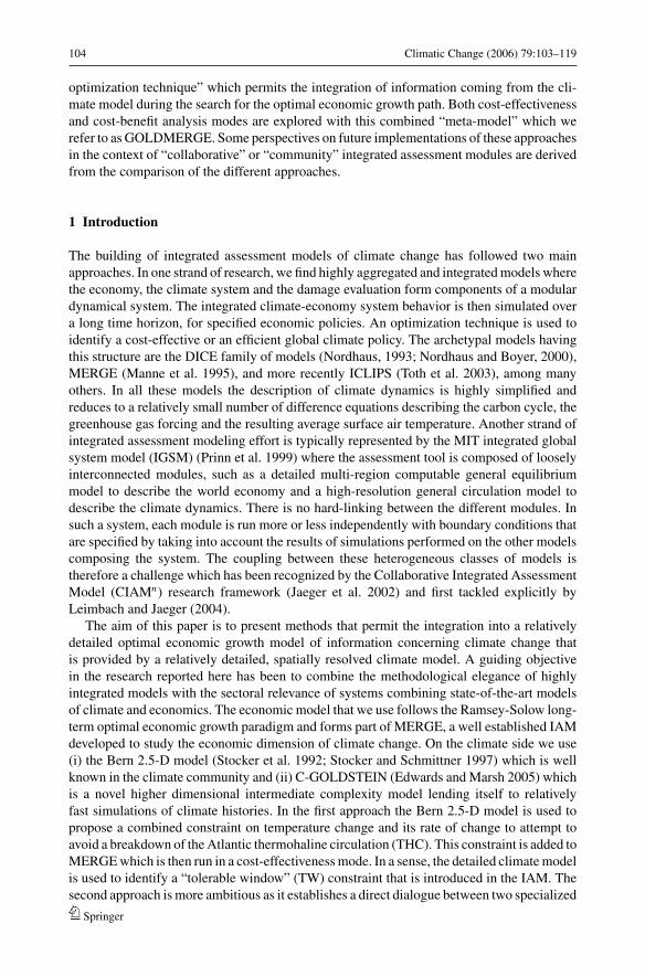
104 Climatic Change (2006) 79:103–119
optimization technique” which permits the integration of information coming from the cli-mate model during the search for the optimal economic growth path. Both cost-effectivenessand cost-benefit analysis modes are explored with this combined “meta-model” which werefer to as GOLDMERGE. Some perspectives on future implementations of these approachesin the context of “collaborative” or “community” integrated assessment modules are derivedfrom the comparison of the different approaches.
1 Introduction
The building of integrated assessment models of climate change has followed two mainapproaches. In one strand of research, we find highly aggregated and integrated models wherethe economy, the climate system and the damage evaluation form components of a modulardynamical system. The integrated climate-economy system behavior is then simulated overa long time horizon, for specified economic policies. An optimization technique is used toidentify a cost-effective or an efficient global climate policy. The archetypal models havingthis structure are the DICE family of models (Nordhaus, 1993; Nordhaus and Boyer, 2000),MERGE (Manne et al. 1995), and more recently ICLIPS (Toth et al. 2003), among manyothers. In all these models the description of climate dynamics is highly simplified andreduces to a relatively small number of difference equations describing the carbon cycle, thegreenhouse gas forcing and the resulting average surface air temperature. Another strand ofintegrated assessment modeling effort is typically represented by the MIT integrated globalsystem model (IGSM) (Prinn et al. 1999) where the assessment tool is composed of looselyinterconnected modules, such as a detailed multi-region computable general equilibriummodel to describe the world economy and a high-resolution general circulation model todescribe the climate dynamics. There is no hard-linking between the different modules. Insuch a system, each module is run more or less independently with boundary conditions thatare specified by taking into account the results of simulations performed on the other modelscomposing the system. The coupling between these heterogeneous classes of models istherefore a challenge which has been recognized by the Collaborative Integrated AssessmentModel (CIAMn) research framework (Jaeger et al. 2002) and first tackled explicitly byLeimbach and Jaeger (2004).
The aim of this paper is to present methods that permit the integration into a relativelydetailed optimal economic growth model of information concerning climate change thatis provided by a relatively detailed, spatially resolved climate model. A guiding objectivein the research reported here has been to combine the methodological elegance of highlyintegrated models with the sectoral relevance of systems combining state-of-the-art modelsof climate and economics. The economic model that we use follows the Ramsey-Solow long-term optimal economic growth paradigm and forms part of MERGE, a well established IAMdeveloped to study the economic dimension of climate change. On the climate side we use(i) the Bern 2.5-D model (Stocker et al. 1992; Stocker and Schmittner 1997) which is wellknown in the climate community and (ii) C-GOLDSTEIN (Edwards and Marsh 2005) whichis a novel higher dimensional intermediate complexity model lending itself to relativelyfast simulations of climate histories. In the first approach the Bern 2.5-D model is used topropose a combined constraint on temperature change and its rate of change to attempt toavoid a breakdown of the Atlantic thermohaline circulation (THC). This constraint is added toMERGE which is then run in a cost-effectiveness mode. In a sense, the detailed climate modelis used to identify a “tolerable window” (TW) constraint that is introduced in the IAM. Thesecond approach is more ambitious as it establishes a direct dialogue between two specialized
Springer
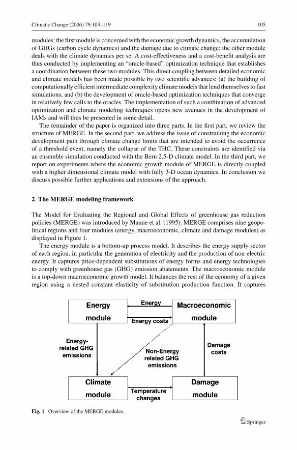
Climatic Change (2006) 79:103–119 105
modules: the first module is concerned with the economic growth dynamics, the accumulationof GHGs (carbon cycle dynamics) and the damage due to climate change; the other moduledeals with the climate dynamics per se. A cost-effectiveness and a cost-benefit analysis arethus conducted by implementing an “oracle-based” optimization technique that establishesa coordination between these two modules. This direct coupling between detailed economicand climate models has been made possible by two scientific advances: (a) the building ofcomputationally efficient intermediate complexity climate models that lend themselves to fastsimulations, and (b) the development of oracle-based optimization techniques that convergein relatively few calls to the oracles. The implementation of such a combination of advancedoptimization and climate modeling techniques opens new avenues in the development ofIAMs and will thus be presented in some detail.
The remainder of the paper is organized into three parts. In the first part, we review thestructure of MERGE. In the second part, we address the issue of constraining the economicdevelopment path through climate change limits that are intended to avoid the occurrenceof a threshold event, namely the collapse of the THC. These constraints are identified viaan ensemble simulation conducted with the Bern 2.5-D climate model. In the third part, wereport on experiments where the economic growth module of MERGE is directly coupledwith a higher dimensional climate model with fully 3-D ocean dynamics. In conclusion wediscuss possible further applications and extensions of the approach.
2 The MERGE modeling framework
The Model for Evaluating the Regional and Global Effects of greenhouse gas reductionpolicies (MERGE) was introduced by Manne et al. (1995). MERGE comprises nine geopo-litical regions and four modules (energy, macroeconomic, climate and damage modules) asdisplayed in Figure 1.
The energy module is a bottom-up process model. It describes the energy supply sectorof each region, in particular the generation of electricity and the production of non-electricenergy. It captures price-dependent substitutions of energy forms and energy technologiesto comply with greenhouse gas (GHG) emission abatements. The macroeconomic moduleis a top-down macroeconomic growth model. It balances the rest of the economy of a givenregion using a nested constant elasticity of substitution production function. It captures
Fig. 1 Overview of the MERGE modules.
Springer
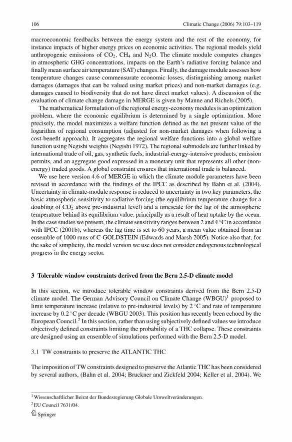
106 Climatic Change (2006) 79:103–119
macroeconomic feedbacks between the energy system and the rest of the economy, forinstance impacts of higher energy prices on economic activities. The regional models yieldanthropogenic emissions of CO2, CH4 and N2O. The climate module computes changesin atmospheric GHG concentrations, impacts on the Earth’s radiative forcing balance andfinally mean surface air temperature (SAT) changes. Finally, the damage module assesses howtemperature changes cause commensurate economic losses, distinguishing among marketdamages (damages that can be valued using market prices) and non-market damages (e.g.damages caused to biodiversity that do not have direct market values). A discussion of theevaluation of climate change damage in MERGE is given by Manne and Richels (2005).
The mathematical formulation of the regional energy-economy modules is an optimizationproblem, where the economic equilibrium is determined by a single optimization. Moreprecisely, the model maximizes a welfare function defined as the net present value of thelogarithm of regional consumption (adjusted for non-market damages when following acost-benefit approach). It aggregates the regional welfare functions into a global welfarefunction using Negishi weights (Negishi 1972). The regional submodels are further linked byinternational trade of oil, gas, synthetic fuels, industrial-energy-intensive products, emissionpermits, and an aggregate good expressed in a monetary unit that represents all other (non-energy) traded goods. A global constraint ensures that international trade is balanced.
We use here version 4.6 of MERGE in which the climate module parameters have beenrevised in accordance with the findings of the IPCC as described by Bahn et al. (2004).Uncertainty in climate-module response is reduced to uncertainty in two key parameters, thebasic atmospheric sensitivity to radiative forcing (the equilibrium temperature change for adoubling of CO2 above pre-industrial level) and a timescale for the lag of the atmospherictemperature behind its equilibrium value, principally as a result of heat uptake by the ocean.In the case studies we present, the climate sensitivity ranges between 2 and 4 ◦C in accordancewith IPCC (2001b), whereas the lag time is set to 60 years, a mean value obtained from anensemble of 1000 runs of C-GOLDSTEIN (Edwards and Marsh 2005). Notice also that, forthe sake of simplicity, the model version we use does not consider endogenous technologicalprogress in the energy sector.
3 Tolerable window constraints derived from the Bern 2.5-D climate model
In this section, we introduce tolerable window constraints derived from the Bern 2.5-Dclimate model. The German Advisory Council on Climate Change (WBGU)1 proposed tolimit temperature increase (relative to pre-industrial levels) by 2 ◦C and rate of temperatureincrease by 0.2 ◦C per decade (WBGU 2003). This position has recently been echoed by theEuropean Council.2 In this section, rather than using subjectively defined values we introduceobjectively defined constraints limiting the probability of a THC collapse. These constraintsare designed using an ensemble of simulations performed with the Bern 2.5-D model.
3.1 TW constraints to preserve the ATLANTIC THC
The imposition of TW constraints designed to preserve the Atlantic THC has been consideredby several authors, (Bahn et al. 2004; Bruckner and Zickfeld 2004; Keller et al. 2004). We
1 Wissenschaftlicher Beirat der Bundesregierung Globale Umweltveranderungen.2 EU Council 7631/04.
Springer
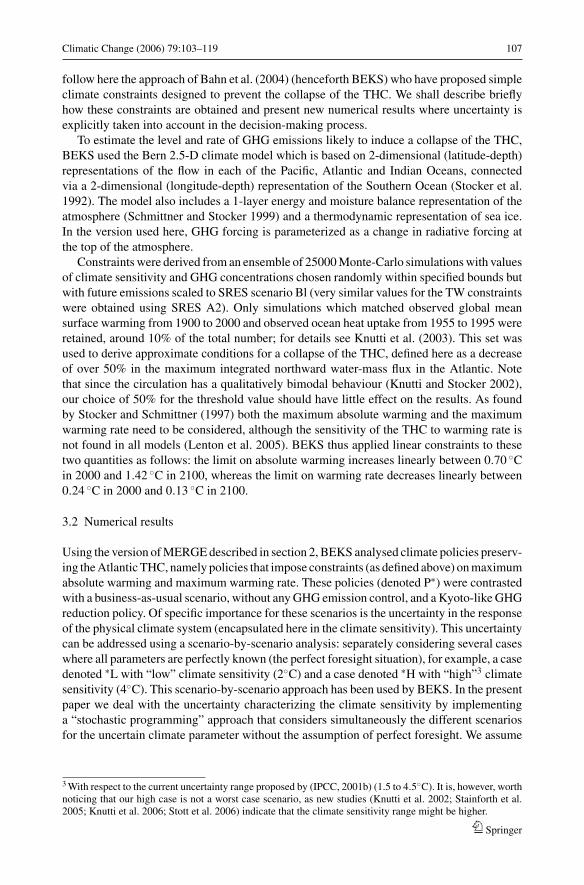
Climatic Change (2006) 79:103–119 107
follow here the approach of Bahn et al. (2004) (henceforth BEKS) who have proposed simpleclimate constraints designed to prevent the collapse of the THC. We shall describe brieflyhow these constraints are obtained and present new numerical results where uncertainty isexplicitly taken into account in the decision-making process.
To estimate the level and rate of GHG emissions likely to induce a collapse of the THC,BEKS used the Bern 2.5-D climate model which is based on 2-dimensional (latitude-depth)representations of the flow in each of the Pacific, Atlantic and Indian Oceans, connectedvia a 2-dimensional (longitude-depth) representation of the Southern Ocean (Stocker et al.1992). The model also includes a 1-layer energy and moisture balance representation of theatmosphere (Schmittner and Stocker 1999) and a thermodynamic representation of sea ice.In the version used here, GHG forcing is parameterized as a change in radiative forcing atthe top of the atmosphere.
Constraints were derived from an ensemble of 25000 Monte-Carlo simulations with valuesof climate sensitivity and GHG concentrations chosen randomly within specified bounds butwith future emissions scaled to SRES scenario Bl (very similar values for the TW constraintswere obtained using SRES A2). Only simulations which matched observed global meansurface warming from 1900 to 2000 and observed ocean heat uptake from 1955 to 1995 wereretained, around 10% of the total number; for details see Knutti et al. (2003). This set wasused to derive approximate conditions for a collapse of the THC, defined here as a decreaseof over 50% in the maximum integrated northward water-mass flux in the Atlantic. Notethat since the circulation has a qualitatively bimodal behaviour (Knutti and Stocker 2002),our choice of 50% for the threshold value should have little effect on the results. As foundby Stocker and Schmittner (1997) both the maximum absolute warming and the maximumwarming rate need to be considered, although the sensitivity of the THC to warming rate isnot found in all models (Lenton et al. 2005). BEKS thus applied linear constraints to thesetwo quantities as follows: the limit on absolute warming increases linearly between 0.70 ◦Cin 2000 and 1.42 ◦C in 2100, whereas the limit on warming rate decreases linearly between0.24 ◦C in 2000 and 0.13 ◦C in 2100.
3.2 Numerical results
Using the version of MERGE described in section 2, BEKS analysed climate policies preserv-ing the Atlantic THC, namely policies that impose constraints (as defined above) on maximumabsolute warming and maximum warming rate. These policies (denoted P∗) were contrastedwith a business-as-usual scenario, without any GHG emission control, and a Kyoto-like GHGreduction policy. Of specific importance for these scenarios is the uncertainty in the responseof the physical climate system (encapsulated here in the climate sensitivity). This uncertaintycan be addressed using a scenario-by-scenario analysis: separately considering several caseswhere all parameters are perfectly known (the perfect foresight situation), for example, a casedenoted ∗L with “low” climate sensitivity (2◦C) and a case denoted ∗H with “high”3 climatesensitivity (4◦C). This scenario-by-scenario approach has been used by BEKS. In the presentpaper we deal with the uncertainty characterizing the climate sensitivity by implementinga “stochastic programming” approach that considers simultaneously the different scenariosfor the uncertain climate parameter without the assumption of perfect foresight. We assume
3 With respect to the current uncertainty range proposed by (IPCC, 2001b) (1.5 to 4.5◦C). It is, however, worthnoticing that our high case is not a worst case scenario, as new studies (Knutti et al. 2002; Stainforth et al.2005; Knutti et al. 2006; Stott et al. 2006) indicate that the climate sensitivity range might be higher.
Springer
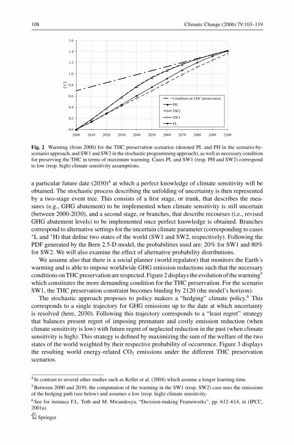
108 Climatic Change (2006) 79:103–119
0.0
0.2
0.4
0.6
0.8
1.0
1.2
1.4
1.6
2000 2010 2020 2030 2040 2050 2060 2070 2080 2090 2100
[°C
]
Condition on THC preservation
PH
SW2
SW1
PL
Fig. 2 Warming (from 2000) for the THC preservation scenarios (denoted PL and PH in the scenario-by-scenario approach, and SW1 and SW2 in the stochastic programming approach), as well as necessary conditionfor preserving the THC in terms of maximum warming. Cases PL and SW1 (resp. PH and SW2) correspondto low (resp. high) climate sensitivity assumptions.
a particular future date (2030)4 at which a perfect knowledge of climate sensitivity will beobtained. The stochastic process describing the unfolding of uncertainty is then representedby a two-stage event tree. This consists of a first stage, or trunk, that describes the mea-sures (e.g., GHG abatement) to be implemented when climate sensitivity is still uncertain(between 2000-2030), and a second stage, or branches, that describe recourses (i.e., revisedGHG abatement levels) to be implemented once perfect knowledge is obtained. Branchescorrespond to alternative settings for the uncertain climate parameter (corresponding to cases∗L and ∗H) that define two states of the world (SW1 and SW2, respectively). Following thePDF generated by the Bern 2.5-D model, the probabilities used are: 20% for SW1 and 80%for SW2. We will also examine the effect of alternative probability distributions.
We assume also that there is a social planner (world regulator) that monitors the Earth’swarming and is able to impose worldwide GHG emission reductions such that the necessaryconditions on THC preservation are respected. Figure 2 displays the evolution of the warming5
which constitutes the more demanding condition for the THC preservation. For the scenarioSW1, the THC preservation constraint becomes binding by 2120 (the model’s horizon).
The stochastic approach proposes to policy makers a “hedging” climate policy.6 Thiscorresponds to a single trajectory for GHG emissions up to the date at which uncertaintyis resolved (here, 2030). Following this trajectory corresponds to a “least regret” strategythat balances present regret of imposing premature and costly emission reduction (whenclimate sensitivity is low) with future regret of neglected reduction in the past (when climatesensitivity is high). This strategy is defined by maximizing the sum of the welfare of the twostates of the world weighted by their respective probability of occurrence. Figure 3 displaysthe resulting world energy-related CO2 emissions under the different THC preservationscenarios.
4 In contrast to several other studies such as Keller et al. (2004) which assume a longer learning time.5 Between 2000 and 2030, the computation of the warming in the SW1 (resp. SW2) case uses the emissionsof the hedging path (see below) and assumes a low (resp. high) climate sensitivity.6 See for instance F.L. Toth and M. Mwandosya, “Decision-making Frameworks”, pp. 612–614, in (IPCC,2001a).
Springer
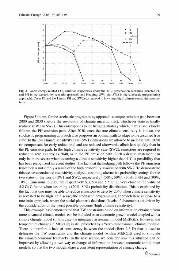
Climatic Change (2006) 79:103–119 109
0
1
2
3
4
5
6
7
8
9
10
2000 2010 2020 2030 2040 2050 2060 2070 2080 2090 2100
[Gt
carb
on p
er y
ear]
PLPHHedgingSW1SW2
Fig. 3 World energy-related CO2 emission trajectories under the THC preservation scenarios (denoted PLand PH in the scenario-by-scenario approach; and Hedging, SW1 and SW2 in the stochastic programmingapproach). Cases PL and SW1 (resp. PH and SW2) correspond to low (resp. high) climate sensitivity assump-tions.
Figure 3 shows, for the stochastic programming approach, a unique emission path between2000 and 2030 (before the resolution of climate uncertainties), whichever state is finallyrealized (SW1 or SW2). This corresponds to the hedging strategy which, in this case, closelyfollows the PH emission path. After 2030, once the true climate sensitivity is known, thestochastic programming approach also proposes an optimal path to adapt to the assumed truestate. In the low climate sensitivity case (SW1), emissions are allowed to increase until 2050(to compensate for early reductions) and are reduced afterwards, albeit less quickly than inthe PL emission path. In the high climate sensitivity case (SW2), emissions are required toreduce to zero as early as 2040, as in the PH emission path. Such a drastic abatement canonly be more severe when assuming a climate sensitivity higher than 4◦C, a possibility thathas been recognized in recent studies. The fact that the hedging path follows the PH emissiontrajectory is not simply a result of the high probability associated with SW2. To demonstratethis we have conducted a sensitivity analysis, assuming alternative probability settings for thetwo states of the world (SW1 and SW2, respectively): (50%, 50%), (70%, 30%) and (90%,10%). Emissions in 2030 are respectively 5.3, 5.4 and 5.5 Gt C, very close to the value of5.2 Gt C found when assuming a (20%, 80%) probability distribution. This is explained bythe fact that one must be able to reduce emissions to zero by 2040 when climate sensitivityis revealed to be high. In a sense, the stochastic programming approach here is close to amaximin approach, where the social planner’s decisions (levels of abatement) are driven bythe consideration of the worst possible outcome (high climate sensitivity).
This example has demonstrated that TW constraints based on information obtained frommore advanced climate models can be included in an economic growth model coupled with asimple climate model (in this case the integrated assessment model MERGE). However, thetemperature change (in MERGE) is still predicted by a “zero-dimensional” climate module.There is therefore a lack of consistency between the model (Bern 2.5-D) that is used todelineate the TW constraints and the climate model (within MERGE) used to simulatethe climate-economy feedbacks. In the next section we consider how this situation can beimproved by allowing a two-way exchange of information between economic and climatemodels, so that the two models share a consistent representation of climate change.
Springer
110 Climatic Change (2006) 79:103–119
4 An oracle-based optimization approach for the coupling of MERGEwith the C-GOLDSTEIN climate model
In this section we describe a general method permitting a coupling between independentand specialized models in order to build an IAM. The method exploits a recently developedmathematical programming method, the “Oracle Based Optimization Technique” (OBOT),that permits a coherent dialogue between models. In the implementation described here, onemodule gives a description of the world economy and carbon-cycle dynamics and is obtainedfrom MERGE. A second module is a 3-D climate model of reduced complexity. The result isan all-encompassing model with an economic sub-model, a climate sub-model and a masterprogram which controls the optimization procedure through a consistent dialogue betweenthe models.
In previous experiments with this approach reported by Drouet et al. (2005a,b) a couplinghas been realized between the economic part of the DICE model and the C-GOLDSTEINclimate model. The implementation of OBOT described here for the coupling of MERGEwith C-GOLDSTEIN represents a significant advance. Not only is MERGE a far morecomprehensive and detailed model of the global energy economy than DICE but furthermore,by coupling climate and economic models both of which have some spatial resolution, wehave made an important step towards an IAM with spatially resolved feedback betweenclimate and economy. In the remainder of this section we first briefly recall the main featuresof the C-GOLDSTEIN model, then present OBOT, the two coupling modes, namely cost-effectiveness (CE) and cost-benefit (CB) and finally the results obtained from this coupling.
4.1 The C-GOLDSTEIN climate model
C-GOLDSTEIN is a flexible geometry, efficient, frictional geostrophic, 3-D global oceanmodel with eddy-induced and isopycnal mixing coupled with an energy and moisture balanceatmosphere and a dynamic and thermodynamic sea-ice component. The model dynamicsand behaviour are described briefly by Drouet et al. (2005a), and more fully by Drouet et al.(2005b). With an integration speed of one or two thousand years per hour on a modern PC(Pentium-IV, 2.4 GHz), it is an order of magnitude less efficient than the Bern 2.5-D model, but3 or 4 orders of magnitude faster than conventional, high-resolution models such as HadCM3(Gordon et al. 2000) and 1 or 2 orders of magnitude faster than other intermediate complexitymodels such as ECBILT-CLIO (Haarsma et al. 2001) or the UVic model (Weaver et al. 2001),which has a very similar atmosphere. This efficiency is mainly a result of low spatial resolutionand simplified dynamics. For the studies described here, the ocean component is configuredwith 8 vertical levels and 36 by 36 cells in the horizontal. Gross features of the global-scaleocean circulation and climate can be reasonably well represented, particularly when modelparameters are automatically calibrated with respect to observational data by performinglarge numbers of simulations (Hargreaves et al. 2005). For the experiments reported here,however, we use default values for model parameters since our focus is on the demonstrationof the coupling technique. All components share the same horizontal grid, but the modelatmosphere has only one vertical level, so that atmospheric processes are represented bya vertical balance of energy and moisture plus simple horizontal transport by anisotropicdiffusion and fixed advection by the wind. Atmospheric radiative forcing is parameterisedby a polynomial function of temperature and humidity with a greenhouse gas forcing termproportional to the log of the ratio of CO2 concentration compared to its pre-industrialvalue. Feedbacks involving changes in atmospheric circulation and precipitation patterns,and feedbacks involving the land surface, are relatively poorly represented or ignored. Sea-ice
Springer

Climatic Change (2006) 79:103–119 111
height and areal coverage are similarly governed by a vertical heat and freshwater balance,plus advection by surface currents with a diffusive term to represent unresolved processes.Given these dynamical simplifications, the model is most suitable for studies of large-scaleocean circulation and long-term climate change, and for probabilistic climate-change studiesand integrated assessment modelling. The model forms a component of the Grid EnabledIntegrated Earth System Model (GENIE) project7 in the context of which an Earth SystemModel with more detailed representations of atmosphere, land-ice, ocean biogeochemistryand land-surface processes is under development.
For the experiments reported here temporal variability in solar forcing is ignored and themodel approaches an equilibrium state, after a few thousand years of integration, which isessentially independent of the initial conditions and can be taken to represent the preindustrialclimate. The model is then integrated forwards with observed atmospheric CO2 concentra-tions from 1795 to 1995 to produce an initial condition for the coupled runs.
4.2 The oracle based optimization technique
The optimization of large-scale systems through decomposition techniques has given rise toimportant developments related to non-differentiable optimization, column generation andcutting plane techniques. The version of an Oracle Based Optimization Technique (OBOT)that we use was first proposed by Goffin et al. (1992). Since then several improvementsand implementation advances have been made as described by Peton and Vial (2001) andBabonneau et al. (2005).
In the world of convex optimization, one searches for the minimum of a convex functionover a convex set of admissible values for the variables. OBOT converges to the optimum bysending a sequence of query points which are proposed values for the decision variables. If thequery point is not feasible (that is, it violates the imposed constraints) an “oracle” sends backinformation in the form of a separating plane which places the query point in one half-spaceand the admissible set in the other. If the query point is feasible, another “oracle” sends backinformation in the form of the value reached by the optimization criterion and the gradientof this function at the query point (which defines a supporting hyperplane for the epigraphof the function). From this sequence of “cutting planes” one is able to construct a polyhedralapproximation of a so-called “localization set” which always contains the optimal values forthe variables and the criterion function. Among possible strategies, one can choose the querypoint at the “center” of the current localization set. The localization set then shrinks rapidlyand it has been proved that the optimum will be found with the desired level of accuracy ina manageable computational time.
The method that we implement is called Analytic Center Cutting Plane Method (ACCPM)in reference to the way one defines the center where one selects the query point. In this method,the criterion and the constraints do not have to be explicitly defined. An implicit definitionpermitting a computation of a value of the function at a query point and an evaluation of itsgradient at this point will suffice. It is this feature which makes the approach very attractiveto couple models pertaining to different spheres.
The convergence of ACCPM towards the global optimum, as well as its rate of conver-gence, has been established for convex optimization problems only. In the present applica-tion, the economic model is convex, but we have no guarantee that the climate model sharesthis property. However, once the two models have found compatible, feasible climate and
7 See http://www.genie.ac.uk
Springer
112 Climatic Change (2006) 79:103–119
emission variables, we can assert that the objective value of the economic model is attainableand provides an upper bound to a global optimum. It may also improve upon alternativelocal optima. This is the situation that prevails at the end of the optimization process in ourapplication.
In proving that the best point found by ACCPM is a local optimum we would face twodifficulties. The first one is that the cutting planes are imprecise as they are computed byfinite differences, and are thus subject to error. The second difficulty stems from the factthat sensitivity analysis in a non-convex model provides information that is only valid ina neighborhood of that point, but may be invalid farther away. To cope with this seconddifficulty, we have implemented a simple scheme that tests whether the cutting plane createdat the current query point invalidates the current best solution. If it does, we simply shift thecutting plane to preserve feasibility of the best solution. This allows for convergence of themethod. In the present case, as well as in the similar applications mentioned earlier, we veryseldom encountered contradictory cutting planes.
Note that even if we could compute exact derivatives in the climate model, local optimalitycould only be guaranteed by discarding remote cutting planes, in the spirit of a trust-regionapproach (More, 1983; Schramm and Zowe, 1992), and proving optimality via local cuttingplanes only. At present, little has been done to extend cutting plane schemes to the non-convex case. Our approach is a pragmatic substitute for a rigorous trust-region scheme,taking into account that the multiple simulations of the climate model required to calculatedamage gradients are computationally expensive, ruling out the possibility of using the largenumbers of query points required by other algorithms such as the differential evolutionalalgorithm considered by Keller et al. (2004).
4.3 Two modes of coupling
We give here briefly the principles of OBOT when applied to the coupling of an eco-nomic growth model with a climate model in two different modes of analysis, namely cost-effectiveness (CE) and cost-benefit (CB) modes. The coupling yields a new meta-IAM whichis now denoted GOLDMERGE-CE or GOLDMERGE-CB according to the coupling modethat is used. The method of solution is similar for the two modes but the information ex-changed between the oracles and the optimization module differs slightly. These differencesand the two reduced-order problems driven by the coupling variables are discussed in the nexttwo subsections. More details on the technical aspects can be found in Drouet et al. (2005a)and Drouet et al. (2005b). We use the economic modules and the carbon-cycle descriptionof MERGE version 4.6 as described in Section 2.
4.3.1 The oracles in the cost-effectiveness mode
In cost-effectiveness mode the coupling variables between the two modules are essentiallythe atmospheric CO2 concentrations, denoted as a vector C with a component for each decadefrom 2010 to 2100. Constraining these variables controls the “economy oracle”. We thus ob-tain an optimal growth path which maximizes the total discounted welfare criterion and sat-isfies these concentration constraints. The sensitivity of the optimized criterion to variationsin the C constraints is provided by duality analysis. The “climate oracle” C-GOLDSTEIN,receiving, as input, the concentration schedule C , computes the average surface air tempera-ture (SAT) and its decadal rate of change. The master program has to find the concentrationschedule C which optimizes the economy under a constraint of 2 ◦C on the average SATchange over the whole planning horizon and 0.2 ◦C on its change over each decade. This
Springer
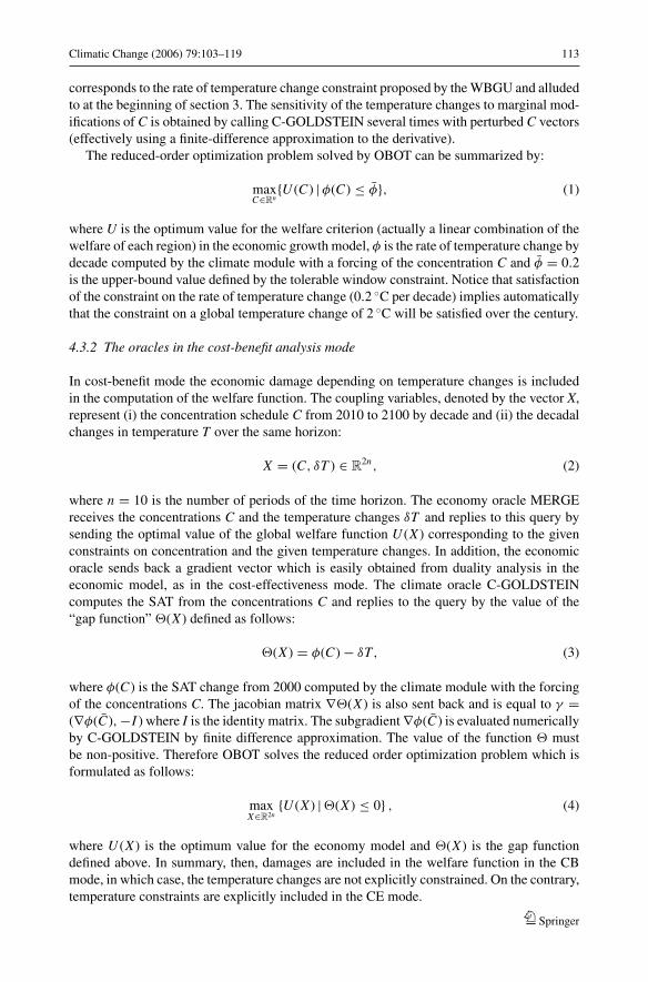
Climatic Change (2006) 79:103–119 113
corresponds to the rate of temperature change constraint proposed by the WBGU and alludedto at the beginning of section 3. The sensitivity of the temperature changes to marginal mod-ifications of C is obtained by calling C-GOLDSTEIN several times with perturbed C vectors(effectively using a finite-difference approximation to the derivative).
The reduced-order optimization problem solved by OBOT can be summarized by:
maxC∈Rn
{U (C) | φ(C) ≤ φ}, (1)
where U is the optimum value for the welfare criterion (actually a linear combination of thewelfare of each region) in the economic growth model, φ is the rate of temperature change bydecade computed by the climate module with a forcing of the concentration C and φ = 0.2is the upper-bound value defined by the tolerable window constraint. Notice that satisfactionof the constraint on the rate of temperature change (0.2 ◦C per decade) implies automaticallythat the constraint on a global temperature change of 2 ◦C will be satisfied over the century.
4.3.2 The oracles in the cost-benefit analysis mode
In cost-benefit mode the economic damage depending on temperature changes is includedin the computation of the welfare function. The coupling variables, denoted by the vector X,represent (i) the concentration schedule C from 2010 to 2100 by decade and (ii) the decadalchanges in temperature T over the same horizon:
X = (C, δT ) ∈ R2n, (2)
where n = 10 is the number of periods of the time horizon. The economy oracle MERGEreceives the concentrations C and the temperature changes δT and replies to this query bysending the optimal value of the global welfare function U (X ) corresponding to the givenconstraints on concentration and the given temperature changes. In addition, the economicoracle sends back a gradient vector which is easily obtained from duality analysis in theeconomic model, as in the cost-effectiveness mode. The climate oracle C-GOLDSTEINcomputes the SAT from the concentrations C and replies to the query by the value of the“gap function” �(X ) defined as follows:
�(X ) = φ(C) − δT, (3)
where φ(C) is the SAT change from 2000 computed by the climate module with the forcingof the concentrations C. The jacobian matrix ∇�(X ) is also sent back and is equal to γ =(∇φ(C), −I ) where I is the identity matrix. The subgradient ∇φ(C) is evaluated numericallyby C-GOLDSTEIN by finite difference approximation. The value of the function � mustbe non-positive. Therefore OBOT solves the reduced order optimization problem which isformulated as follows:
maxX∈R2n
{U (X ) | �(X ) ≤ 0} , (4)
where U (X ) is the optimum value for the economy model and �(X ) is the gap functiondefined above. In summary, then, damages are included in the welfare function in the CBmode, in which case, the temperature changes are not explicitly constrained. On the contrary,temperature constraints are explicitly included in the CE mode.
Springer
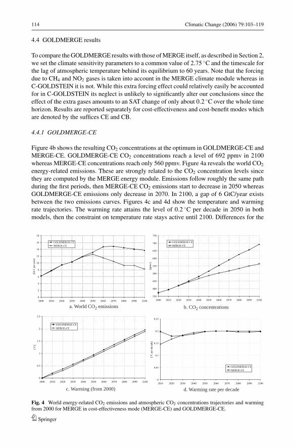
114 Climatic Change (2006) 79:103–119
4.4 GOLDMERGE results
To compare the GOLDMERGE results with those of MERGE itself, as described in Section 2,we set the climate sensitivity parameters to a common value of 2.75 ◦C and the timescale forthe lag of atmospheric temperature behind its equilibrium to 60 years. Note that the forcingdue to CH4 and NO2 gases is taken into account in the MERGE climate module whereas inC-GOLDSTEIN it is not. While this extra forcing effect could relatively easily be accountedfor in C-GOLDSTEIN its neglect is unlikely to significantly alter our conclusions since theeffect of the extra gases amounts to an SAT change of only about 0.2 ◦C over the whole timehorizon. Results are reported separately for cost-effectiveness and cost-benefit modes whichare denoted by the suffices CE and CB.
4.4.1 GOLDMERGE-CE
Figure 4b shows the resulting CO2 concentrations at the optimum in GOLDMERGE-CE andMERGE-CE. GOLDMERGE-CE CO2 concentrations reach a level of 692 ppmv in 2100whereas MERGE-CE concentrations reach only 560 ppmv. Figure 4a reveals the world CO2
energy-related emissions. These are strongly related to the CO2 concentration levels sincethey are computed by the MERGE energy module. Emissions follow roughly the same pathduring the first periods, then MERGE-CE CO2 emissions start to decrease in 2050 whereasGOLDMERGE-CE emissions only decrease in 2070. In 2100, a gap of 6 GtC/year existsbetween the two emissions curves. Figures 4c and 4d show the temperature and warmingrate trajectories. The warming rate attains the level of 0.2 ◦C per decade in 2050 in bothmodels, then the constraint on temperature rate stays active until 2100. Differences for the
0
2
4
6
8
10
12
14
16
18
2000 2010 2020 2030 2040 2050 2060 2070 2080 2090 2100
[Gt C
per
yea
r]
GOLDMERGE-CEMERGE-CE
350
400
450
500
550
600
650
700
750
2000 2010 2020 2030 2040 2050 2060 2070 2080 2090 2100
[ppm
v]
GOLDMERGE-CEMERGE-CE
0
0.5
1
1.5
2
2.5
2000 2010 2020 2030 2040 2050 2060 2070 2080 2090 2100
[°C
]
GOLDMERGE-CEMERGE-CE
0
0.05
0.1
0.15
0.2
0.25
2010 2020 2030 2040 2050 2060 2070 2080 2090 2100
[°C
per
dec
ade]
GOLDMERGE-CEMERGE-CE
a. World CO2 emissions b. CO2 concentrations
c. Warming (from 2000) d. Warming rate per decade
Fig. 4 World energy-related CO2 emissions and atmospheric CO2 concentrations trajectories and warmingfrom 2000 for MERGE in cost-effectiveness mode (MERGE-CE) and GOLDMERGE-CE.
Springer
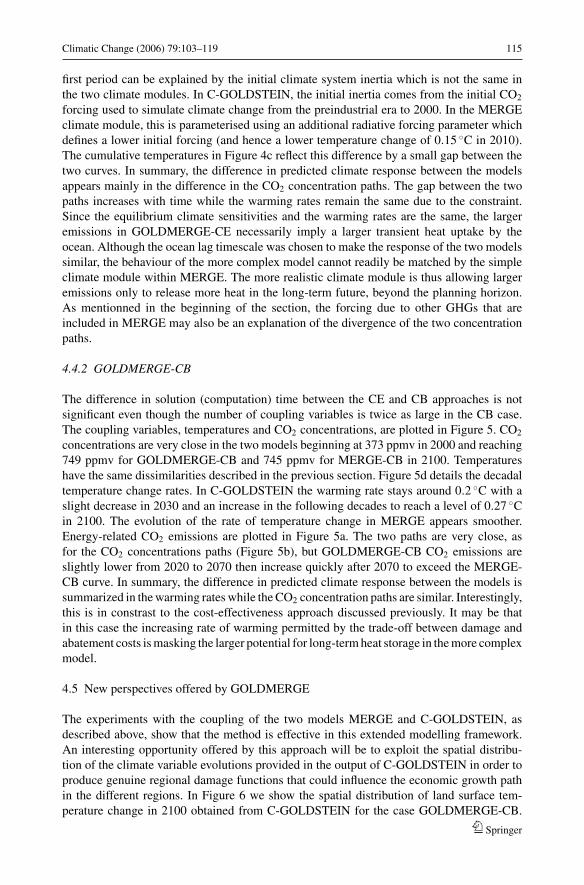
Climatic Change (2006) 79:103–119 115
first period can be explained by the initial climate system inertia which is not the same inthe two climate modules. In C-GOLDSTEIN, the initial inertia comes from the initial CO2
forcing used to simulate climate change from the preindustrial era to 2000. In the MERGEclimate module, this is parameterised using an additional radiative forcing parameter whichdefines a lower initial forcing (and hence a lower temperature change of 0.15 ◦C in 2010).The cumulative temperatures in Figure 4c reflect this difference by a small gap between thetwo curves. In summary, the difference in predicted climate response between the modelsappears mainly in the difference in the CO2 concentration paths. The gap between the twopaths increases with time while the warming rates remain the same due to the constraint.Since the equilibrium climate sensitivities and the warming rates are the same, the largeremissions in GOLDMERGE-CE necessarily imply a larger transient heat uptake by theocean. Although the ocean lag timescale was chosen to make the response of the two modelssimilar, the behaviour of the more complex model cannot readily be matched by the simpleclimate module within MERGE. The more realistic climate module is thus allowing largeremissions only to release more heat in the long-term future, beyond the planning horizon.As mentionned in the beginning of the section, the forcing due to other GHGs that areincluded in MERGE may also be an explanation of the divergence of the two concentrationpaths.
4.4.2 GOLDMERGE-CB
The difference in solution (computation) time between the CE and CB approaches is notsignificant even though the number of coupling variables is twice as large in the CB case.The coupling variables, temperatures and CO2 concentrations, are plotted in Figure 5. CO2
concentrations are very close in the two models beginning at 373 ppmv in 2000 and reaching749 ppmv for GOLDMERGE-CB and 745 ppmv for MERGE-CB in 2100. Temperatureshave the same dissimilarities described in the previous section. Figure 5d details the decadaltemperature change rates. In C-GOLDSTEIN the warming rate stays around 0.2 ◦C with aslight decrease in 2030 and an increase in the following decades to reach a level of 0.27 ◦Cin 2100. The evolution of the rate of temperature change in MERGE appears smoother.Energy-related CO2 emissions are plotted in Figure 5a. The two paths are very close, asfor the CO2 concentrations paths (Figure 5b), but GOLDMERGE-CB CO2 emissions areslightly lower from 2020 to 2070 then increase quickly after 2070 to exceed the MERGE-CB curve. In summary, the difference in predicted climate response between the models issummarized in the warming rates while the CO2 concentration paths are similar. Interestingly,this is in constrast to the cost-effectiveness approach discussed previously. It may be thatin this case the increasing rate of warming permitted by the trade-off between damage andabatement costs is masking the larger potential for long-term heat storage in the more complexmodel.
4.5 New perspectives offered by GOLDMERGE
The experiments with the coupling of the two models MERGE and C-GOLDSTEIN, asdescribed above, show that the method is effective in this extended modelling framework.An interesting opportunity offered by this approach will be to exploit the spatial distribu-tion of the climate variable evolutions provided in the output of C-GOLDSTEIN in order toproduce genuine regional damage functions that could influence the economic growth pathin the different regions. In Figure 6 we show the spatial distribution of land surface tem-perature change in 2100 obtained from C-GOLDSTEIN for the case GOLDMERGE-CB.
Springer
116 Climatic Change (2006) 79:103–119
0
2
4
6
8
10
12
14
16
18
20
22
24
26
2000 2010 2020 2030 2040 2050 2060 2070 2080 2090 2100
[Gt C
per
yea
r]
GOLDMERGE-CBMERGE-CB
350
400
450
500
550
600
650
700
750
800
2000 2010 2020 2030 2040 2050 2060 2070 2080 2090 2100
[ppm
v]
GOLDMERGE-CBMERGE-CB
0
0.5
1
1.5
2
2.5
2000 2010 2020 2030 2040 2050 2060 2070 2080 2090 2100
[°C
]
GOLDMERGE-CBMERGE-CB
0
0.05
0.1
0.15
0.2
0.25
0.3
0.35
2010 2020 2030 2040 2050 2060 2070 2080 2090 2100
[°C
per
dec
ade]
GOLDMERGE-CB
MERGE-CB
a. World CO2 emissions b. CO2 concentrations
c. Warming (from 2000) d. Warming rate per decade
Fig. 5 World energy-related CO2 emissions and atmospheric CO2 concentrations trajectories and warmingfrom 2000 for MERGE in cost-benefit mode (MERGE-CB) and GOLDMERGE-CB.
Fig. 6 Distribution of the temperature increase for the standard MERGE regions in 2100 for GOLDMERGE-CB.
Regionalized temperature increases lie within a range from 1.76 ◦C to 2.25 ◦C. Another im-portant remark concerns the compatibility of the approach with the use of TW constraints.Indeed, since the climate model is sufficiently detailed, the THC shutdown phenomenonis implicitly represented in it. By imposing regionalized “viability” constraints8 on purely
8 See (Aubin et al. 2005) for a discussion of viability methods in climate modeling.
Springer
Climatic Change (2006) 79:103–119 117
climatic variables like precipitation, temperature, ice and snow cover etc. a tolerable windowsapproach to climate change policies could be defined based on relatively detailed economicand climate models, while still maintaining computational feasibility. The method could inprinciple be utilised for the coupling of any optimal economic growth model with any gen-eral circulation model. Limitations remain in computation time and model convexity. Thiskind of coupling is highly relevant for community based assessment because it effectivelyresolves the problem of the inclusion of complex simulation models inside an optimizationframework. To conduct a similar exercise with a high-resolution climate model with a de-tailed and realistic regional temperature and precipitation response would require significantcomputational resources, but the knowledge which would be gained may well justify such aninvestment.
5 Conclusion
In this paper we have presented two different ways to establish a dialogue between a climatemodel and an economic model in order to obtain an integrated assessment of climate policies.First we have shown how a TW constraint can be introduced in the MERGE integratedassessment model in a cost-effectiveness fashion to attempt to prevent the occurrence ofa drastic THC weakening. Our TW constraint was obtained from ensemble simulationsperformed with a spatially resolved climate model (the Bern 2.5-D model) to delineate theconditions that would prevent a THC shutdown. This approach has the advantage of usinginformation coming from a reliable climate model to introduce a TW constraint in MERGE.The climate response to the GHG emissions coming from the economy is however derivedfrom the simplified and schematic climate module that is included in MERGE. In the secondexample developed here we have described an approach to realize a hard link between aneconomic growth module and a 3-D climate model of reduced complexity. This approachyields interesting results when the economic growth, carbon cycle and damage modulesof MERGE are coupled with the intermediate complexity 3D-model C-GOLDSTEIN. In areasonable computing time (a few hours on a 2.4 GHz Intel machine) it has been possible toproduce consistent simulations of economic growth and climate change paths in either cost-effectiveness or cost-benefit analysis frameworks (the GOLDMERGE-CE and -CB models).The tool that has been used to realize the coupling (OBOT) implements an optimizationmethod using “oracles” that correspond to different models.
The results reported here pave the way to the building of more comprehensive and moredetailed IAMs. Currently the method is being tested for a coupling between the economicpart of MERGE and CBM-GOLDSTEIN (GENIE-1), a more advanced climate model in-cluding a description of the carbon cycle. It will also be possible to exploit the fact thatthe climate model gives a spatially distributed view of the evolution of climate variables.This should permit us to build regional damage functions or to link climate feedbacks withthe economic activity (e.g. agriculture). The method could also be extended to realize acoupling between the macroeconomic growth module and a more detailed techno-economicmodel of the energy sector, in addition to the coupling with a moderate complexity climatemodel.
Acknowledgements The authors acknowledge financial support by the Natural Sciences and EngineeringResearch Council of Canada, the Swiss National Science Foundation, and the Swiss National Centre forCompetence in Research, NCCR climate.
Springer
118 Climatic Change (2006) 79:103–119
References
Aubin J-P, Bernardo T, Saint-Pierre P (2005) A viability approach to global climate change issues. In: HaurieA and Viguier L (eds.) The coupling of climate and economic dynamics. Kluwer, pp 113–140
Babonneau F, Beltran C, Haurie A, Tadonki C, Vial J-P (2005) Proximal-ACCPM: a versatile oracle basedoptimization method. Computational and Management Science. Submitted.
Bahn O, Edwards N, Knutti R, Stocker T (2004) Climate policy preserving an atlantic thermohaline circulationcollapse. Climatic Change. Submitted. Available in Les Cahiers du GERAD, reference G-2004-72
Bruckner T, Zickfeld K (2004) Low risk emissions corridors for safeguarding the atlantic thermohaline cir-culation. In: paper presented at the Expert Workshop “Greenhouse Gas Emissions and Abrupt ClimateChange”, Paris.
Drouet L, Beltran C, Edwards N, Haurie A, Vial J-P, Zachary D (2005a) An oracle method to couple climate andeconomic dynamics. In: Haurie A and Viguier L (eds.) The coupling of climate and economic dynamics.Kluwer pp 69–94
Drouet L, Edwards N, Haurie (2005b) Coupling climate and economic models in a cost-benefit framework: aconvex optimization approach. Environmental Modeling and Assessment. Submitted.
Edwards N, Marsh R (2005) Uncertainties due to transport-parameter sensitivity in an efficient 3-D ocean-climate model. Climate Dynamics 24:415–433
Goffin J-L, Haurie A, Vial J-P (1992) Decomposition and non-differentiable optimization with the projectivealgorithm. Management Science 38:284–302
Gordon C, Cooper C, Senior C, Banks H, Gregory J, Johns T, Mitchell J, Wood R (2000) The simulation ofSST, sea-ice extents and ocean heat transports in a version of the Hadley Centre coupled model withoutflux adjustments. Climate Dynamics 16:147–168
Haarsma R, Goosse H, Selten F, Opsteegh JD (2001) Decadal variability in high northern latitudes as simulatedby an intermediate-complexity climate model. Annals of Glaciology 33:525–532
Hargreaves J, Annan J, Edwards N, Marsh R (2005) Climate forecasting using an intermediate complexityearth system model and the ensemble kalman filter. Climate Dynamics 23(7–8):745–760
IPCC (2001a) Climate change 2001: mitigation, contribution of working group III to the third assessmentreport of the intergovernmental panel on climate change. Metz B et al. (eds) Cambridge University Press.Cambridge, U.K.
IPCC (2001b) Climate change 2001: the scientific basis, contribution of working group I to the third assessmentreport of the intergovernmental panel on climate change. Houghtom J et al. (eds) Cambridge UniversityPress, Cambridge, U.K.
Jaeger CC, Leimbach M, Carraro C, Hasselmann K, Hourcade JC, Keeler A, Klein R (2002) Integratedassessment modeling: modules for cooperation. FEEM Working Paper No. 53
Keller K, Bolker B, Bradford D (2004) Uncertain climate thresholds and optimal economic growth. Journalof Environmental Economics and Management 48(1):723–741
Knutti R, Meehl G, Allen MR, Stain forth DA (2005) Constraining climate sensitivity from the seasonal cyclein surface temperature. J. Climate 19:4224–4233
Knutti R, Stocker T (2002) Limited predictability of the future thermohaline circulation close to an instabilitythreshold. Journal of Climate 15:179–186
Knutti R, Stocker T, Joos F, Plattner G-K (2002) Constraints on radiative forcing and future climate changefrom observations and climate model ensembles. Nature 416:719–723
Knutti R, Stocker TF, Joos F, Plattner G-K (2003) Probabilistic climate change projections using neuralnetworks. Climate Dynamics 21:257–272
Leimbach M, Jaeger C (2004) A modular approach to integrated assessment modeling. Environmental Mod-elling and Assessment 9(4):207–220
Lenton TM, Williamson MS, Edwards NR, Marsh R, Price AR, Ridgwell AJ, Shepherd JG, and the GENIEteam (2005) Millennial timescale carbon cycle and climate change in an efficient Earth system model.Climate Dynamics. Submitted.
Manne A, Mendelsohn R, Richels R (1995) MERGE - a model for evaluating regional and global effects ofGHG reduction policies. Energy Policy 23(1):17–34
Manne A, Richels R (2005) MERGE: an integrated assessment model for global climate change. In: LoulouR, Waaub J-P, Zaccour G, (eds) Energy and Environment. GERAD 25th Anniversary Series. Springer, pp175–189
More J (1983) Recent developments in algorithms and software for trust region methods. In: MathematicalProgramming: The State of the Art. Springer Verlag, Berlin, pp. 258–287
Negishi T (1972) General equilibrium theory and international trade. North-Holland.Nordhaus W (1993) Rolling the ‘DICE’: an optimal transition path for controlling greenhouse gases. Resource
and Energy Economics 15:27–50
Springer
Climatic Change (2006) 79:103–119 119
Nordhaus W, Boyer J (2000) Warming the world: economic models of global warming. MIT PressPeton O, Vial J-P (2001) A brief tutorial on ACCPM. Technical report. Logilab, University of GenevaPrinn R, et al. (1999) Integrated global system model for climate policy assessment: feedbacks and sensitivity
studies. Climatic Change 3/4(41):469–546Schmittner A, Stocker T (1999) The stability of the thermohaline circulation in global warming experiments.
Journal of Climate 12:1117–1133Schramm H, Zowe J (1992) A version of the bundle idea for minimizing a non-smooth function: conceptual
idea, convergence analysis, numerical results. SIAM Journal on Optimization 2:121–152Stainforth D, et al (2005) Uncertainty in predictions of the climate response to rising levels of greenhouse
gases. Nature 433:403–406Stocker T, Schmittner A (1997) Influence of CO2 emissions rates on the stability of the thermohaline circulation.
Nature 388:862–865Stocker T, Wright D, Mysak L (1992) A zonally averaged, coupled ocean-atmosphere model for paleoclimate
studies. Journal of Climate 4:773–797Stott P, Mitchell J, Gregory J, Santer B, Meehl G, Delworth T, Allen M (2005) Observational constraints on
past attributable warming and predictions of future global warming. J. Climate 19:3055–3069Toth F, Bruckner T, Fuessel H-M, Leimbach M, Petshel-Held G (2003) Integrated assessment of long-term
climate policies: part 1 – model presentation. Climatic Change 56:37–56WBGU (2003) Climate protection strategies for the 21st century. Earthscan, London.Weaver A, Eby M, Wiebe E, Bitz C, Duffy P, Ewen T, Fanning A, Holland M, MacFadyen A, Matthews
H, Meissner K, Saenko O, Schmittner A, Wang H, Yoshimori M (2001) The UVic earth system climatemodel: model description, climatology, and applications to past, present and future climates. Atmos-Ocean39:361–428
Springer
Climatic Change (2006) 79:121–141DOI 10.1007/s10584-006-9070-1
Modeling endogenous learning and imperfectcompetition effects in climate change economics
Laurent Viguier · Leonardo Barreto · Alain Haurie ·Socrates Kypreos · Peter Rafaj
Received: 26 October 2004 / Accepted: 9 November 2005 / Published online: 13 October 2006C© Springer Science + Business Media B.V. 2006
Abstract In this two-part paper we evaluate the effect of “endogenizing” technologicallearning and strategic behavior of agents in economic models used to assess climate changepolicies. In the first part we show the potential impact of R&D policies or demonstrationand deployment (D&D) programs in the context of stringent stabilization scenarios. In thesecond part we show how game-theoretic methods can be implemented in climate changeeconomic models to take into account three types of strategic interactions: (i) the marketpower of the countries benefiting from very low abatement costs on international marketsfor CO2 emissions, (ii) the strategic behavior of governments in the domestic allocation ofCO2 emissions quotas, and (iii) the non-cooperative behavior of countries and regions in theburden sharing of CO2 concentration stabilization. The two topics of endogenous learningand game-theoretic approach to economic modeling are two manifestations of the need totake into account the strategic behavior of agents in the evaluation of climate change policies.In the first case an R&D policy or a demonstration and deployment (D&D) program are putin place in order to attain a cost reduction through the learning effect; in the second case theagents (countries) reply optimally to the actions decided by the other agents by exploitingtheir strategic advantages. Simulations based on integrated assessment models illustrate theapproaches. These studies have been conducted under the Swiss NCCR-Climate program.
Keywords Endogenous technological learning . Strategic behavior . Climate policy .
Emissions trading . Economic models . Dynamic games
L. Viguier (�)Ecole Polytechnique Federale de Lausanne (EPFL), Switzerland; MIT Joint Program on the Science andPolicy of Global Change, Cambridge, MA, USAe-mail: [email protected]
L. Barreto · S. KypreosPaul Scherrer Institute, Villigen, Switzerland
A. HaurieHEC-Geneva, Switzerland
P. RafajInternational Institute for Applied Systems Analysis, Laxenburg, Austria
Springer
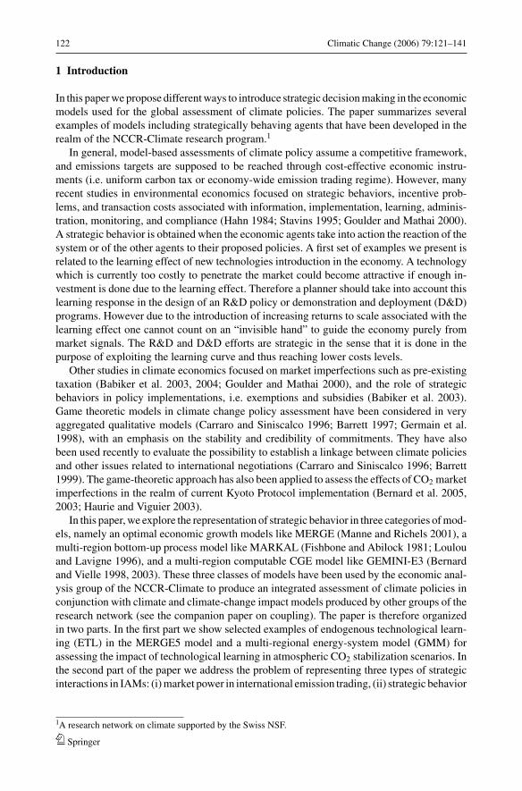
122 Climatic Change (2006) 79:121–141
1 Introduction
In this paper we propose different ways to introduce strategic decision making in the economicmodels used for the global assessment of climate policies. The paper summarizes severalexamples of models including strategically behaving agents that have been developed in therealm of the NCCR-Climate research program.1
In general, model-based assessments of climate policy assume a competitive framework,and emissions targets are supposed to be reached through cost-effective economic instru-ments (i.e. uniform carbon tax or economy-wide emission trading regime). However, manyrecent studies in environmental economics focused on strategic behaviors, incentive prob-lems, and transaction costs associated with information, implementation, learning, adminis-tration, monitoring, and compliance (Hahn 1984; Stavins 1995; Goulder and Mathai 2000).A strategic behavior is obtained when the economic agents take into action the reaction of thesystem or of the other agents to their proposed policies. A first set of examples we present isrelated to the learning effect of new technologies introduction in the economy. A technologywhich is currently too costly to penetrate the market could become attractive if enough in-vestment is done due to the learning effect. Therefore a planner should take into account thislearning response in the design of an R&D policy or demonstration and deployment (D&D)programs. However due to the introduction of increasing returns to scale associated with thelearning effect one cannot count on an “invisible hand” to guide the economy purely frommarket signals. The R&D and D&D efforts are strategic in the sense that it is done in thepurpose of exploiting the learning curve and thus reaching lower costs levels.
Other studies in climate economics focused on market imperfections such as pre-existingtaxation (Babiker et al. 2003, 2004; Goulder and Mathai 2000), and the role of strategicbehaviors in policy implementations, i.e. exemptions and subsidies (Babiker et al. 2003).Game theoretic models in climate change policy assessment have been considered in veryaggregated qualitative models (Carraro and Siniscalco 1996; Barrett 1997; Germain et al.1998), with an emphasis on the stability and credibility of commitments. They have alsobeen used recently to evaluate the possibility to establish a linkage between climate policiesand other issues related to international negotiations (Carraro and Siniscalco 1996; Barrett1999). The game-theoretic approach has also been applied to assess the effects of CO2 marketimperfections in the realm of current Kyoto Protocol implementation (Bernard et al. 2005,2003; Haurie and Viguier 2003).
In this paper, we explore the representation of strategic behavior in three categories of mod-els, namely an optimal economic growth models like MERGE (Manne and Richels 2001), amulti-region bottom-up process model like MARKAL (Fishbone and Abilock 1981; Loulouand Lavigne 1996), and a multi-region computable CGE model like GEMINI-E3 (Bernardand Vielle 1998, 2003). These three classes of models have been used by the economic anal-ysis group of the NCCR-Climate to produce an integrated assessment of climate policies inconjunction with climate and climate-change impact models produced by other groups of theresearch network (see the companion paper on coupling). The paper is therefore organizedin two parts. In the first part we show selected examples of endogenous technological learn-ing (ETL) in the MERGE5 model and a multi-regional energy-system model (GMM) forassessing the impact of technological learning in atmospheric CO2 stabilization scenarios. Inthe second part of the paper we address the problem of representing three types of strategicinteractions in IAMs: (i) market power in international emission trading, (ii) strategic behavior
1A research network on climate supported by the Swiss NSF.
Springer
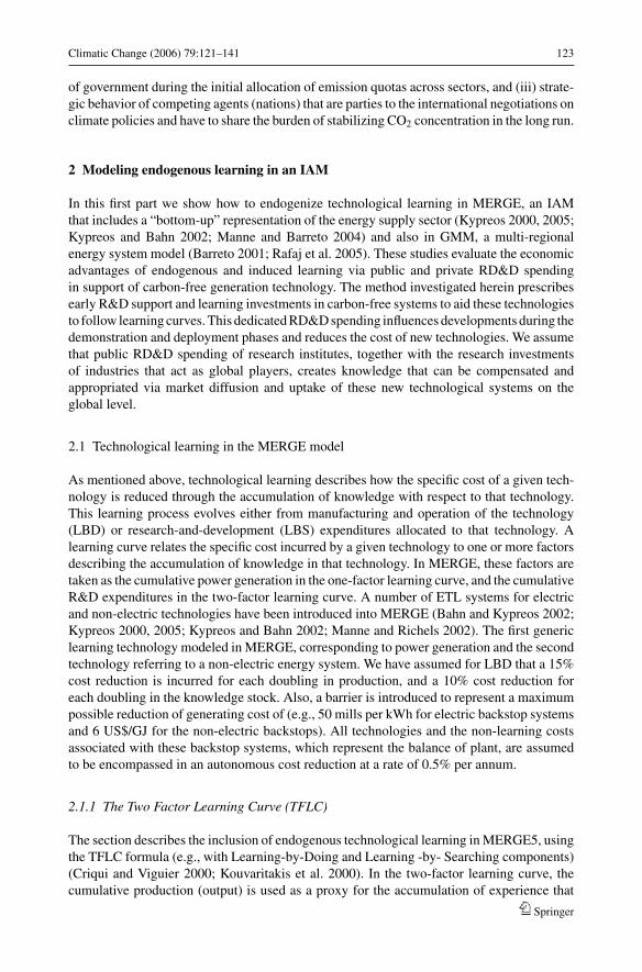
Climatic Change (2006) 79:121–141 123
of government during the initial allocation of emission quotas across sectors, and (iii) strate-gic behavior of competing agents (nations) that are parties to the international negotiations onclimate policies and have to share the burden of stabilizing CO2 concentration in the long run.
2 Modeling endogenous learning in an IAM
In this first part we show how to endogenize technological learning in MERGE, an IAMthat includes a “bottom-up” representation of the energy supply sector (Kypreos 2000, 2005;Kypreos and Bahn 2002; Manne and Barreto 2004) and also in GMM, a multi-regionalenergy system model (Barreto 2001; Rafaj et al. 2005). These studies evaluate the economicadvantages of endogenous and induced learning via public and private RD&D spendingin support of carbon-free generation technology. The method investigated herein prescribesearly R&D support and learning investments in carbon-free systems to aid these technologiesto follow learning curves. This dedicated RD&D spending influences developments during thedemonstration and deployment phases and reduces the cost of new technologies. We assumethat public RD&D spending of research institutes, together with the research investmentsof industries that act as global players, creates knowledge that can be compensated andappropriated via market diffusion and uptake of these new technological systems on theglobal level.
2.1 Technological learning in the MERGE model
As mentioned above, technological learning describes how the specific cost of a given tech-nology is reduced through the accumulation of knowledge with respect to that technology.This learning process evolves either from manufacturing and operation of the technology(LBD) or research-and-development (LBS) expenditures allocated to that technology. Alearning curve relates the specific cost incurred by a given technology to one or more factorsdescribing the accumulation of knowledge in that technology. In MERGE, these factors aretaken as the cumulative power generation in the one-factor learning curve, and the cumulativeR&D expenditures in the two-factor learning curve. A number of ETL systems for electricand non-electric technologies have been introduced into MERGE (Bahn and Kypreos 2002;Kypreos 2000, 2005; Kypreos and Bahn 2002; Manne and Richels 2002). The first genericlearning technology modeled in MERGE, corresponding to power generation and the secondtechnology referring to a non-electric energy system. We have assumed for LBD that a 15%cost reduction is incurred for each doubling in production, and a 10% cost reduction foreach doubling in the knowledge stock. Also, a barrier is introduced to represent a maximumpossible reduction of generating cost of (e.g., 50 mills per kWh for electric backstop systemsand 6 US$/GJ for the non-electric backstops). All technologies and the non-learning costsassociated with these backstop systems, which represent the balance of plant, are assumedto be encompassed in an autonomous cost reduction at a rate of 0.5% per annum.
2.1.1 The Two Factor Learning Curve (TFLC)
The section describes the inclusion of endogenous technological learning in MERGE5, usingthe TFLC formula (e.g., with Learning-by-Doing and Learning -by- Searching components)(Criqui and Viguier 2000; Kouvaritakis et al. 2000). In the two-factor learning curve, thecumulative production (output) is used as a proxy for the accumulation of experience that
Springer
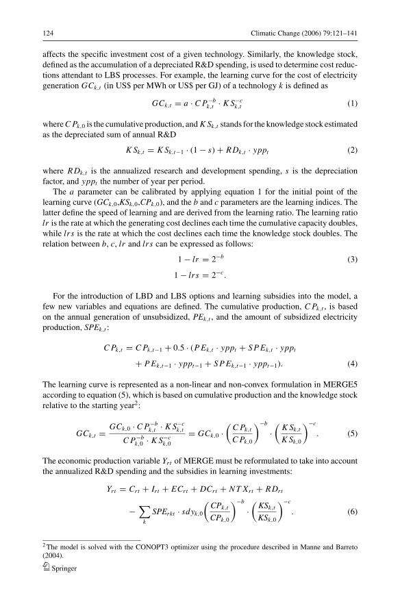
124 Climatic Change (2006) 79:121–141
affects the specific investment cost of a given technology. Similarly, the knowledge stock,defined as the accumulation of a depreciated R&D spending, is used to determine cost reduc-tions attendant to LBS processes. For example, the learning curve for the cost of electricitygeneration GCk,t (in US$ per MWh or US$ per GJ) of a technology k is defined as
GCk,t = a · C P−bk,t · K S−c
k,t (1)
where C Pk,0 is the cumulative production, and K Sk,t stands for the knowledge stock estimatedas the depreciated sum of annual R&D
K Sk,t = K Sk,t−1 · (1 − s) + RDk,t · yppt (2)
where RDk,t is the annualized research and development spending, s is the depreciationfactor, and yppt the number of year per period.
The a parameter can be calibrated by applying equation 1 for the initial point of thelearning curve (GCk,0,KSk,0,CPk,0), and the b and c parameters are the learning indices. Thelatter define the speed of learning and are derived from the learning ratio. The learning ratiolr is the rate at which the generating cost declines each time the cumulative capacity doubles,while lrs is the rate at which the cost declines each time the knowledge stock doubles. Therelation between b, c, lr and lrs can be expressed as follows:
1 − lr = 2−b (3)
1 − lrs = 2−c.
For the introduction of LBD and LBS options and learning subsidies into the model, afew new variables and equations are defined. The cumulative production, C Pk,t , is basedon the annual generation of unsubsidized, PEk,t , and the amount of subsidized electricityproduction, SPEk,t :
C Pk,t = C Pk,t−1 + 0.5 · (P Ek,t · yppt + S P Ek,t · yppt
+ P Ek,t−1 · yppt−1 + S P Ek,t−1 · yppt−1). (4)
The learning curve is represented as a non-linear and non-convex formulation in MERGE5according to equation (5), which is based on cumulative production and the knowledge stockrelative to the starting year2:
GCk,t = GCk,0 · C P−bk,t · K S−c
k,t
C P−bk,0 · K S−c
k,0
= GCk,0 ·(
C Pk,t
C Pk,0
)−b
·(
K Sk,t
K Sk,0
)−c
. (5)
The economic production variable Yrt of MERGE must be reformulated to take into accountthe annualized R&D spending and the subsidies in learning investments:
Yrt = Crt + Irt + ECrt + DCrt + N T Xrt + RDrt
−∑
k
SPErkt · sdyk,0
(CPk,t
CPk,0
)−b
·(
KSk,t
KSk,0
)−c
. (6)
2 The model is solved with the CONOPT3 optimizer using the procedure described in Manne and Barreto(2004).
Springer
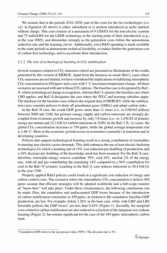
Climatic Change (2006) 79:121–141 125
We assume that in the periods 2010–2030, part of the costs for the two technologies (i.e.sdy in Equation (6) above) is either subsidized or is anyhow introduced in niche marketswithout charge. This cost consists of a maximum of 9 US$/GJ for the non-electric systemsand 75 mills/kWh for the LBDE technology at the starting point of their introduction (e.g.,in the year 2005), and diminishes strongly as the generation costs follow the autonomousreduction rate and the learning curves. Additionally, extra R&D spending is made availablein the same periods to demonstrate technical feasibility, to reduce further the generation costof carbon-free technology, and to accelerate their introduction.
2.1.2 The role of technological learning in CO2 stabilization
Several scenarios related to CO2 emission control are presented as illustrations of the resultsgenerated by this version of MERGE. Apart from the business-as-usual (BaU), cases whereCO2 emissions are not limited, we have considered the implications of stabilizing atmosphericCO2 concentration to 450 ppmv and a case with 2 ◦C maximum temperature change. All threescenarios are assessed with and without ETL options. The baseline case is designated by BaU-N, where technological change is exogenous, whereas BaU-L denotes the baseline case whereLBD applies, and BaU-S designates the case where the TFLC and learning subsidies apply.The database for the baseline cases reflects the original data of MERGE5, while the stabiliza-tion cases consider policies to abate all greenhouse gases (GHGs) and adopt carbon sinks.
In the BaU-N case, the world GDP grows more than 11 times (i.e., to US$365 trillion)between 2000 and 2100; but primary-energy supply and carbon emissions are strongly de-coupled from economic growth and increase by only 3.8 times (i.e., to 1,430 EJ of primaryenergy per annum and 22.3 GtC/yr carbon emissions in 2100). In the BaU (-N, -L) cases, theglobal CO2 concentration increases to 750 ppmv, while the global average temperature riseis 2.48 ◦C. Most of the economic growth occurs in economies (currently) in transition and indeveloping countries.
Policies that support technological learning result in a strong contribution of renewablesin meeting non-electric-sector demands. This shift enhances the use of non-electric backstoptechnologies for which a learning rate of 15% cost reduction per doubling of production, anda 10% decrease per doubling of the knowledge stock has been assumed. For the BaU-S case,therefore, renewable-energy sources contribute 39%, coal 45%, nuclear 2% of the energymix, with oil and gas contributing the remaining 14% compared to a 56% contribution forcoal in the BaU-N scenario. Learning in the BaU-L case reduces emissions to 20.4 GtC/yrin the year 2100.
Properly applied R&D policies could result in a significant cost reduction of energy andcarbon control costs. The scenarios where the atmospheric CO2 concentration is held to 450ppmv assume that efficient strategies will be adopted worldwide and a full-scope transferof ”know-how” will take place. Under these circumstances, the following conclusions canbe made: First, the cumulative and undiscounted GDP losses because of the introductionof carbon-stabilization constraints at 450 ppmv, in relation to the cumulative baseline-GDPproduction, are low. For example, below 1.26% in the base case, while with LBD and LBSfavorable policies the GDP losses3 are less than 0.42% (Figure 1). Secondly, the marginalcosts related to carbon stabilization are also reduced to a fraction of the marginal cost withoutlearning (Figure 2), but remain significant for the case of the 450 ppmv atmospheric carbonlimit.
3 Cumulative GDP refers to the net present value (NPV). The discount rate is 5%.
Springer
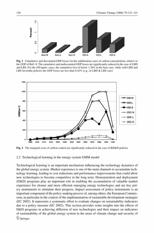
126 Climatic Change (2006) 79:121–141
Fig. 1 Cumulative and discounted GDP losses for the stabilization cases of carbon concentration, relative tothe GDP of BaU-S. The cumulative and undiscounted GDP losses are significantly reduced in the case of LBDand LBS. For the 450-ppmv cases, the cumulative loss of below 1.26% in the base case, while with LBD andLBS favorable policies the GDP losses are less than 0.42% (e.g., in LBD & LBS case)
Fig. 2 The marginal costs of carbon control are significantly reduced in the case of RD&D policies
2.2 Technological learning in the energy-system GMM model
Technological learning is an important mechanism influencing the technology dynamics ofthe global energy system. Market experience is one of the main channels to accumulate tech-nology learning, leading to cost reductions and performance improvements that could allownew technologies to become competitive in the long term. Demonstration and deployment(D&D) programs play an important role in enabling the accumulation of valuable marketexperience for cleaner and more efficient emerging energy technologies and are key pol-icy instruments to stimulate their progress. Impact assessment of policy instruments is animportant component of the policy-making process of, among others, the European Commis-sion, in particular in the context of the implementation of sustainable development strategies(EC 2002). It represents a systematic effort to evaluate changes on sustainability indicatorsdue to a policy measure (EC 2002). This section provides some insights into the effects ofD&D programs in achieving diffusion of new technologies and their impact on indicatorsof sustainability of the global energy system in the areas of climate change and security of
Springer
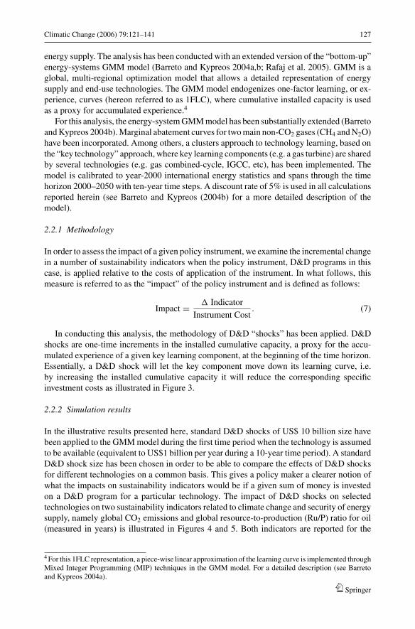
Climatic Change (2006) 79:121–141 127
energy supply. The analysis has been conducted with an extended version of the “bottom-up”energy-systems GMM model (Barreto and Kypreos 2004a,b; Rafaj et al. 2005). GMM is aglobal, multi-regional optimization model that allows a detailed representation of energysupply and end-use technologies. The GMM model endogenizes one-factor learning, or ex-perience, curves (hereon referred to as 1FLC), where cumulative installed capacity is usedas a proxy for accumulated experience.4
For this analysis, the energy-system GMM model has been substantially extended (Barretoand Kypreos 2004b). Marginal abatement curves for two main non-CO2 gases (CH4 and N2O)have been incorporated. Among others, a clusters approach to technology learning, based onthe “key technology” approach, where key learning components (e.g. a gas turbine) are sharedby several technologies (e.g. gas combined-cycle, IGCC, etc), has been implemented. Themodel is calibrated to year-2000 international energy statistics and spans through the timehorizon 2000–2050 with ten-year time steps. A discount rate of 5% is used in all calculationsreported herein (see Barreto and Kypreos (2004b) for a more detailed description of themodel).
2.2.1 Methodology
In order to assess the impact of a given policy instrument, we examine the incremental changein a number of sustainability indicators when the policy instrument, D&D programs in thiscase, is applied relative to the costs of application of the instrument. In what follows, thismeasure is referred to as the “impact” of the policy instrument and is defined as follows:
Impact = � Indicator
Instrument Cost. (7)
In conducting this analysis, the methodology of D&D “shocks” has been applied. D&Dshocks are one-time increments in the installed cumulative capacity, a proxy for the accu-mulated experience of a given key learning component, at the beginning of the time horizon.Essentially, a D&D shock will let the key component move down its learning curve, i.e.by increasing the installed cumulative capacity it will reduce the corresponding specificinvestment costs as illustrated in Figure 3.
2.2.2 Simulation results
In the illustrative results presented here, standard D&D shocks of US$ 10 billion size havebeen applied to the GMM model during the first time period when the technology is assumedto be available (equivalent to US$1 billion per year during a 10-year time period). A standardD&D shock size has been chosen in order to be able to compare the effects of D&D shocksfor different technologies on a common basis. This gives a policy maker a clearer notion ofwhat the impacts on sustainability indicators would be if a given sum of money is investedon a D&D program for a particular technology. The impact of D&D shocks on selectedtechnologies on two sustainability indicators related to climate change and security of energysupply, namely global CO2 emissions and global resource-to-production (Ru/P) ratio for oil(measured in years) is illustrated in Figures 4 and 5. Both indicators are reported for the
4 For this 1FLC representation, a piece-wise linear approximation of the learning curve is implemented throughMixed Integer Programming (MIP) techniques in the GMM model. For a detailed description (see Barretoand Kypreos 2004a).
Springer
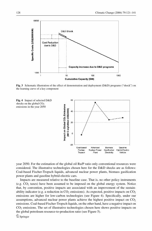
128 Climatic Change (2006) 79:121–141
Fig. 3 Schematic illustration of the effect of demonstration and deployment (D&D) programs (“shock”) onthe learning curve of a key component
Fig. 4 Impact of selected D&Dshocks on the global CO2emissions in the year 2050
year 2050. For the estimation of the global oil Ru/P ratio only conventional resources wereconsidered. The illustrative technologies chosen here for the D&D shocks are as follows:Coal-based Fischer-Tropsch liquids, advanced nuclear power plants, biomass gasificationpower plants and gasoline hybrid-electric cars.
Impacts are measured relative to the baseline case. That is, no other policy instruments(e.g. CO2 taxes) have been assumed to be imposed on the global energy system. Noticethat, by convention, positive impacts are associated with an improvement of the sustain-ability indicator (e.g. a reduction in CO2 emissions). As expected, positive impacts on CO2
emissions are higher for low-carbon technologies (see Figure 4). Specifically, under ourassumptions, advanced nuclear power plants achieve the highest positive impact on CO2
emissions. Coal-based Fischer-Tropsch liquids, on the other hand, have a negative impact onCO2 emissions. The set of illustrative technologies chosen here shows positive impacts onthe global petroleum resource-to-production ratio (see Figure 5).
Springer
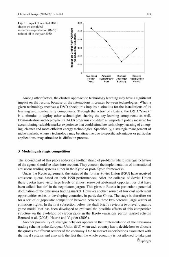
Climatic Change (2006) 79:121–141 129
Fig. 5 Impact of selected D&Dshocks on the globalresources-to-production (Ru/P)ratio of oil in the year 2050
Among other factors, the clusters approach to technology learning may have a significantimpact on the results, because of the interactions it creates between technologies. When agiven technology receives a D&D shock, this implies a stimulus for the installations of itslearning and non-learning components. Through the action of clusters, the D&D “shock”is a stimulus to deploy other technologies sharing the key learning components as well.Demonstration and deployment (D&D) programs constitute an important policy measure foraccumulating valuable market experience that could stimulate technology learning of emerg-ing, cleaner and more efficient energy technologies. Specifically, a strategic management ofniche markets, where a technology may be attractive due to specific advantages or particularapplications, may stimulate its diffusion process.
3 Modeling strategic competition
The second part of this paper addresses another strand of problems where strategic behaviorof the agents should be taken into account. They concern the implementation of internationalemissions trading systems either in the Kyoto or post-Kyoto frameworks.
Under the Kyoto agreement, the states of the former Soviet Union (FSU) have receivedemissions quotas based on their 1990 performances. After the collapse of Soviet Unionthese quotas have yield large levels of almost zero-cost abatement opportunities that havebeen called “hot air” in the negotiators jargon. This gives to Russia in particular a potentialdomination of the emissions trading market. However another source of low cost abatementopportunities exists in developing countries, in particular China. The stage is therefore setfor a sort of oligopolistic competition between between these two potential large sellers ofemissions rights. In the first subsection below we shall briefly review a two-level dynamicgame model that has been developed to evaluate the possible effects of this competitivestructure on the evolution of carbon price in the Kyoto emissions permit market schemeBernard et al. (2005); Haurie and Viguier (2003).
Another possibility of strategic behavior appears in the implementation of the emissionstrading scheme in the European Union (EU) when each country has to decide how to allocatethe quotas to different sectors of the economy. Due to market imperfections associated withthe fiscal systems and also with the fact that the whole economy is not allowed to take part
Springer
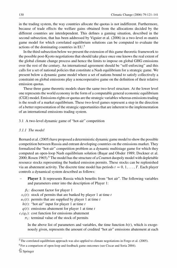
130 Climatic Change (2006) 79:121–141
in the trading system, the way countries allocate the quotas is not indifferent. Furthermore,because of trade effects the welfare gains obtained from the allocations decided by thedifferent countries are interdependent. This defines a gaming situation, described in thesecond subsection, that has been addressed by Viguier et al. (2006) in a two-level m-matrixgame model for which correlated equilibrium solutions can be computed to evaluate theactions of the dominating countries in EU.5
In the third subsection below we present the extension of this game theoretic framework tothe possible post-Kyoto negotiations that should take place once one knows the real extent ofthe global climate change process and hence the limits to impose on global GHG emissionsover the rest of the century. An international agreement should be “self-enforcing” and thiscalls for a set of national policies that constitute a Nash equilibrium for a strategic game. Wepresent below a dynamic game model where a set of nations bound to satisfy collectively aconstraint on global emissions play a noncooperative game on the definition of their relativeemission quotas.
These three game theoretic models share the same two-level structure. At the lower levelone represents the world economy in the form of a computable general economic equilibrium(CGE) model. Emissions rights or quotas are the strategic variables whereas emissions tradingis the result of a market equilibrium. These two-level games represent a step in the directionof a better representation of the strategic opportunities that are inherent to the implementationof an international emissions trading system.
3.1 A two-level dynamic game of “hot-air” competition
3.1.1 The model
Bernard et al. (2005) have proposed a deterministic dynamic game model to show the possiblecompetition between Russia and entrant developing countries on the emissions market. Theyformalized the “hot-air” competition problem as a dynamic multistage game for which theycomputed an open-loop Nash equilibrium solution (Basar and Olsder 1989; Dockner et al.2000; Rosen 1965).6 The model has the structure of a Cournot duopoly model with depletableresource stocks representing the banked emission permits. These stocks can be replenishedvia an abatement activity. The discrete time model has periods t = 0, 1, . . . , T . Each playercontrols a dynamical system described as follows:
– Player 1: It represents Russia which benefits from “hot air”. The following variablesand parameters enter into the description of Player 1:
β1: discount factor for player 1x1(t): stock of permits that are banked by player 1 at time tu1(t): permits that are supplied by player 1 at time th(t): “hot air” input for player 1 at time tq(t): emissions abatement for player 1 at time t
c1(q1): cost function for emissions abatementπ1: terminal value of the stock of permits
In the above list of parameters and variables, the time function h(t), which is exoge-nously given, represents the amount of credited “hot air” emissions abatement at each
5 The correlated equilibrium approach was also applied to climate negotiations in Forgo et al. (2005).6 For a comparison of open-loop and feedback game outcomes (see Ciscar and Soria 2004).
Springer

Climatic Change (2006) 79:121–141 131
time t . We assume h(t) ≥ 0 if t < T and h(T ) = 0. The dynamical system representingPlayer 1 is defined as follows:
maxT −1∑t=0
β t1[p(t)u1(t) − c1(q1(t))] + βT
1 π1x1(T ) (8)
s.t. x1(t + 1) = x1(t) − u1(t) + h(t) + q1(t) (9)
x1(0) = 0 (10)
u1(t) ≥ 0 (11)
x1(t) ≥ 0. (12)
– Player 2: It represents a large developing country (typically China) which may developits own market of emission rights instead of the CDM scheme. The following variablesand parameters enter into the description of Player 2:
β2: discount factor for player 2x2(t): stock of permits that are banked by player 2 at time tu2(t): permits that are supplied by player 2 at time tq2(t): emissions decrease due to Player 2 abatement activities
c2(q2): cost function for emissions abatementπ2: terminal value of the stock of permitsθ : period at which China may join the market
The dynamical system representing Player 2 is defined as follows:
maxT −1∑t=0
β t2[p(t)u1(t) − c2(q2(t))] + βT
2 π2x2(T ) (13)
s.t. x2(t + 1) = x2(t) − u2(t) + q2(t) (14)
x2(0) = 0 (15)
u2(t) ≥ 0 (16)
u2(t) ≡ 0 ∀t ∈ [0, θ] where θ < T (17)
x2(t) ≥ 0. (18)
– Price of permits: An inverse demand law describes the market clearing price forpermits in Annex B countries.
p(t) = D(u1(t) + u2(t)). (19)
This demand function is derived from the competitive equilibrium conditions for theAnnex B countries in each period.
We look for a Nash equilibrium solution, assuming an open-loop information structure (thereader is referred to Basar and Olsder (1989) for a presentation of the information structures indynamic games). It means that the competing agents select an open-loop control, that is a timeschedule for their supply of emission permits over the planning horizon 0, 1, . . . , T − 1. Theoptimality conditions are obtained by formulating the first order Nash equilibrium conditions.
Springer
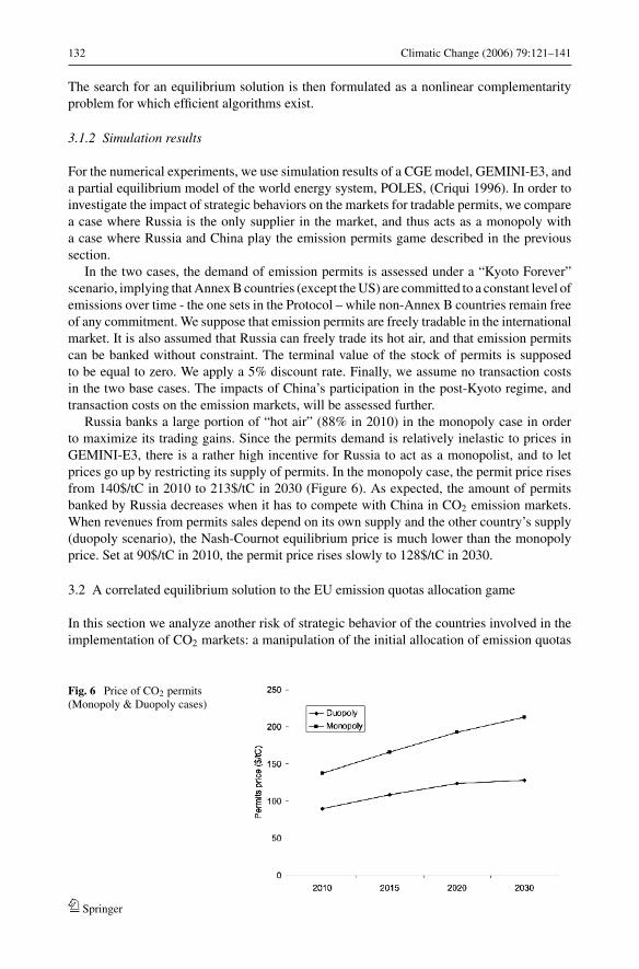
132 Climatic Change (2006) 79:121–141
The search for an equilibrium solution is then formulated as a nonlinear complementarityproblem for which efficient algorithms exist.
3.1.2 Simulation results
For the numerical experiments, we use simulation results of a CGE model, GEMINI-E3, anda partial equilibrium model of the world energy system, POLES, (Criqui 1996). In order toinvestigate the impact of strategic behaviors on the markets for tradable permits, we comparea case where Russia is the only supplier in the market, and thus acts as a monopoly witha case where Russia and China play the emission permits game described in the previoussection.
In the two cases, the demand of emission permits is assessed under a “Kyoto Forever”scenario, implying that Annex B countries (except the US) are committed to a constant level ofemissions over time - the one sets in the Protocol – while non-Annex B countries remain freeof any commitment. We suppose that emission permits are freely tradable in the internationalmarket. It is also assumed that Russia can freely trade its hot air, and that emission permitscan be banked without constraint. The terminal value of the stock of permits is supposedto be equal to zero. We apply a 5% discount rate. Finally, we assume no transaction costsin the two base cases. The impacts of China’s participation in the post-Kyoto regime, andtransaction costs on the emission markets, will be assessed further.
Russia banks a large portion of “hot air” (88% in 2010) in the monopoly case in orderto maximize its trading gains. Since the permits demand is relatively inelastic to prices inGEMINI-E3, there is a rather high incentive for Russia to act as a monopolist, and to letprices go up by restricting its supply of permits. In the monopoly case, the permit price risesfrom 140$/tC in 2010 to 213$/tC in 2030 (Figure 6). As expected, the amount of permitsbanked by Russia decreases when it has to compete with China in CO2 emission markets.When revenues from permits sales depend on its own supply and the other country’s supply(duopoly scenario), the Nash-Cournot equilibrium price is much lower than the monopolyprice. Set at 90$/tC in 2010, the permit price rises slowly to 128$/tC in 2030.
3.2 A correlated equilibrium solution to the EU emission quotas allocation game
In this section we analyze another risk of strategic behavior of the countries involved in theimplementation of CO2 markets: a manipulation of the initial allocation of emission quotas
Fig. 6 Price of CO2 permits(Monopoly & Duopoly cases)
Springer
Climatic Change (2006) 79:121–141 133
in order to subsidize their energy-intensive industries. One should represent the problem asa non-cooperative game and look for some equilibrium solution. As explained in Viguieret al. (2006), this game has a two-level structure since the strategies selected by the playershave consequences that are calculated from a computable general equilibrium model. Theupper-level game is represented as an M-matrix game, where M is the set of active countriesand where the payoffs are obtained by running a CGE model (i.e. GEMINI-E3) under theconfigurations associated with the different possible strategy choices. The upper-level gamewill be solved for the characterization of the set of correlated equilibria (see Aumann 1974).
3.2.1 The model
The games is played by countries or groups of countries that may manipulate the initialallocation of emission quotas. The strategies are the different (contrasted) allocation schemesthat could result from individual decisions over quotas allocation. The payoffs of the gameare the welfare gains (-losses) for each player resulting from Kyoto emission targets under theEU-wide trading regime. Again, we say that these games have a two-level structure since thestrategies selected by the players have consequences that are calculated from a computablegeneral equilibrium model. The upper-level game is represented as an M-matrix game, whereM is the set of active countries and where the payoffs are obtained by running GEMINI-E3under the configurations associated with the different possible strategy choices. The upper-level game is solved for the characterization of the set of correlated equilibria. The game instrategic form is defined by = (M, (Sj ) j∈M , (u j ) j∈M ) where M is the set of players, Sj isthe set of our strategies of player j and u j : i∈M Si → R is the payoff function for player j .Let us denote S = i∈M Si and s = (s j ) j∈M ∈ S. A correlated equilibrium is defined by aprobability distribution on S, π (s) ≥ 0,
∑s∈S π (s) = 1 such that the following inequalities
hold
∑s∈S
π (s)u j (s) ≥∑s∈S
π (s)u j (s− j , σ j ), ∀ j ∈ M, ∀ σ j ∈ Sj . (20)
where
(s− j , σ j ) = (si , . . . , s j−1, σ j , s j+1, . . . , sm) (21)
and M = 1, . . . , m.The interpretation can be the following: through a preplay communication scheme the
agents may exchange signals that sum up to each player receiving a recommendation to playa given strategy. The probability π (s) is affected to the event: the vector s is recommendedas a way to play the game. We have to realize that, in this interpretation, each player knowsonly the recommendation to play that concerns him. The inequalities (20) express the factthat a player has no incentive to play other than as recommended.
In brief we could view a correlated equilibrium either as the result of playing a gamewhere a mediator sends private information to each player, in the form of a recommendationto play a given strategy, or as the result of the use of communication strategies by the players,where each player would send reports to the other players (and receive reports from theothers) before deciding what to do. We can see the relevance of this scheme in the contextof EU-wide negotiation for the implementation of a tradable emission permit scheme.
It is well known that the set of correlated equilibria in an M-matrix game is closedand compact and can be characterized through the solution of linear programs. The set of
Springer
134 Climatic Change (2006) 79:121–141
correlated equilibria contains the set of Nash equilibria. Therefore, if this set of correlatedequilibria reduces to a singleton, it is the unique Nash equilibria for the game.
3.2.2 Simulation results
The allocation of CO2 emission quotas in the implementation of the EU-wide emissiontrading market can be viewed as an example of a “permits allocation game”. Viguier et al.(2006) represent this situation as an M-matrix game, where the strategic players are Germany(DEU), the United Kingdom (UK), Italy (ITA), and the rest of the European Union (REU).We assume that these regions may choose among four different rules to allocate emissionallowances across economic sectors:
1. Grandfathering (GF): Emission allowances are allocated among sectors according totheir historical emissions taking into account a global target of emissions reduction atthe national level;
2. Historical emissions (HE): The total number of allowances allocated to a given tradingsector is determined by its share in each Member Stateís emissions from economicsectors included in the trading scheme emitted in a particular year (e.g. 2001), multipliedby total allowable emissions for the economy;
3. Domestic Tax-based (DT): Sectoral allowances correspond to the ones that would occurif a uniform carbon tax were to be implemented at the domestic level;
4. European Tax-based (ET): Sectoral allowances correspond to the ones that would occurif a uniform carbon tax were to be implemented at the European level.
We simulate three different games with four players and three strategies. In Game 1,one assumes that the reference rule for quotas allocation corresponds to the one equalizingmarginal abatement costs across sectors at the domestic level (DT). We assess the incentivefor EU countries to deviate from the DT allocation by giving 10 percent more (or less) quotasto the trading sector. In Game 2, the players can choose among more contrasted strategies.We allow EU countries to deviate a little bit more from the DT approach by giving more(GF) or less (e.g. ET in Germany) quotas to the trading sector. In Game 3, the only way forEU countries to strategize on the allocation of quotas is to give more quotas to the tradingsector; the GF approach corresponds to a lower deviation from the ET rule than the HEapproach.
In our numerical experiments it turns out that the games have a unique correlated equi-librium which then corresponds to a unique Nash equilibrium in pure (instead of mixed)strategies (see Table 1). The equilibria are always different from the competitive equilibriumsolutions, where the different regions would play the same DT strategy. Germany, which isthe main supplier of emission allowances, tends to rely on the domestic tax-based approach(DT) but the other regions, which are permits buyers, have an incentive to depart from thisapproach to maximize their own payoffs. The outcomes of the non-cooperative equilibria
Table 1 Unique correlatedequilibria Game 1 Game 2 Game 3
Germany DT DT DT
UK DT−10 GF GF
Italy DT+10 DT HE
Rest of EU-15 DT+10 GF GF
Springer
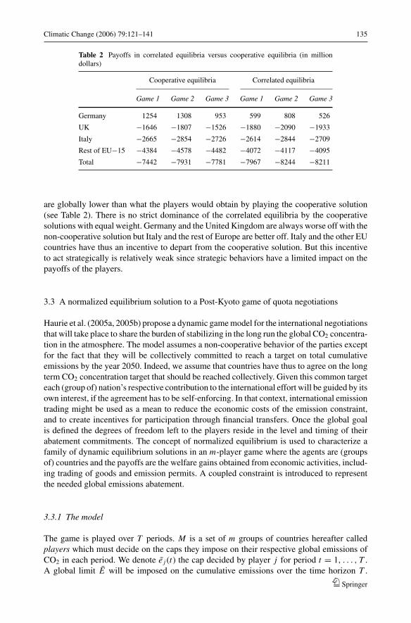
Climatic Change (2006) 79:121–141 135
Table 2 Payoffs in correlated equilibria versus cooperative equilibria (in milliondollars)
Cooperative equilibria Correlated equilibria
Game 1 Game 2 Game 3 Game 1 Game 2 Game 3
Germany 1254 1308 953 599 808 526
UK −1646 −1807 −1526 −1880 −2090 −1933
Italy −2665 −2854 −2726 −2614 −2844 −2709
Rest of EU−15 −4384 −4578 −4482 −4072 −4117 −4095
Total −7442 −7931 −7781 −7967 −8244 −8211
are globally lower than what the players would obtain by playing the cooperative solution(see Table 2). There is no strict dominance of the correlated equilibria by the cooperativesolutions with equal weight. Germany and the United Kingdom are always worse off with thenon-cooperative solution but Italy and the rest of Europe are better off. Italy and the other EUcountries have thus an incentive to depart from the cooperative solution. But this incentiveto act strategically is relatively weak since strategic behaviors have a limited impact on thepayoffs of the players.
3.3 A normalized equilibrium solution to a Post-Kyoto game of quota negotiations
Haurie et al. (2005a, 2005b) propose a dynamic game model for the international negotiationsthat will take place to share the burden of stabilizing in the long run the global CO2 concentra-tion in the atmosphere. The model assumes a non-cooperative behavior of the parties exceptfor the fact that they will be collectively committed to reach a target on total cumulativeemissions by the year 2050. Indeed, we assume that countries have thus to agree on the longterm CO2 concentration target that should be reached collectively. Given this common targeteach (group of) nation’s respective contribution to the international effort will be guided by itsown interest, if the agreement has to be self-enforcing. In that context, international emissiontrading might be used as a mean to reduce the economic costs of the emission constraint,and to create incentives for participation through financial transfers. Once the global goalis defined the degrees of freedom left to the players reside in the level and timing of theirabatement commitments. The concept of normalized equilibrium is used to characterize afamily of dynamic equilibrium solutions in an m-player game where the agents are (groupsof) countries and the payoffs are the welfare gains obtained from economic activities, includ-ing trading of goods and emission permits. A coupled constraint is introduced to representthe needed global emissions abatement.
3.3.1 The model
The game is played over T periods. M is a set of m groups of countries hereafter calledplayers which must decide on the caps they impose on their respective global emissions ofCO2 in each period. We denote e j (t) the cap decided by player j for period t = 1, . . . , T .A global limit E will be imposed on the cumulative emissions over the time horizon T .
Springer
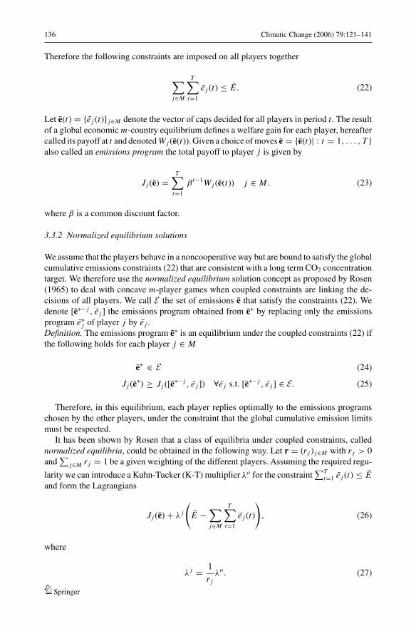
136 Climatic Change (2006) 79:121–141
Therefore the following constraints are imposed on all players together
∑j∈M
T∑t=1
e j (t) ≤ E . (22)
Let e(t) = {e j (t)} j∈M denote the vector of caps decided for all players in period t . The resultof a global economic m-country equilibrium defines a welfare gain for each player, hereaftercalled its payoff at t and denoted W j (e(t)). Given a choice of moves e = {e(t)| : t = 1, . . . , T }also called an emissions program the total payoff to player j is given by
Jj (e) =T∑
t=1
β t−1W j (e(t)) j ∈ M. (23)
where β is a common discount factor.
3.3.2 Normalized equilibrium solutions
We assume that the players behave in a noncooperative way but are bound to satisfy the globalcumulative emissions constraints (22) that are consistent with a long term CO2 concentrationtarget. We therefore use the normalized equilibrium solution concept as proposed by Rosen(1965) to deal with concave m-player games when coupled constraints are linking the de-cisions of all players. We call E the set of emissions e that satisfy the constraints (22). Wedenote [e∗− j , e j ] the emissions program obtained from e∗ by replacing only the emissionsprogram e∗
j of player j by e j .Definition. The emissions program e∗ is an equilibrium under the coupled constraints (22) ifthe following holds for each player j ∈ M
e∗ ∈ E (24)
Jj (e∗) ≥ Jj ([e∗− j , e j ]) ∀e j s.t. [e∗− j , e j ] ∈ E . (25)
Therefore, in this equilibrium, each player replies optimally to the emissions programschosen by the other players, under the constraint that the global cumulative emission limitsmust be respected.
It has been shown by Rosen that a class of equilibria under coupled constraints, callednormalized equilibria, could be obtained in the following way. Let r = (r j ) j∈M with r j > 0and
∑j∈M r j = 1 be a given weighting of the different players. Assuming the required regu-
larity we can introduce a Kuhn-Tucker (K-T) multiplier λo for the constraint∑T
t=1 e j (t) ≤ Eand form the Lagrangians
Jj (e) + λ j
(E −
∑j∈M
T∑t=1
e j (t)
), (26)
where
λ j = 1
r jλo. (27)
Springer
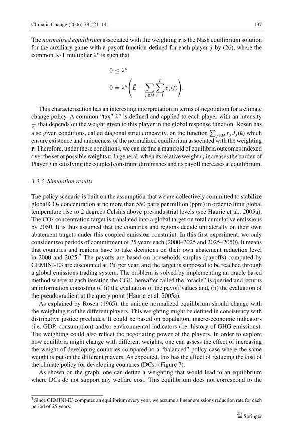
Climatic Change (2006) 79:121–141 137
The normalized equilibrium associated with the weighting r is the Nash equilibrium solutionfor the auxiliary game with a payoff function defined for each player j by (26), where thecommon K-T multiplier λo is such that
0 ≤ λo
0 = λo
(E −
∑j∈M
T∑t=1
e j (t)
).
This characterization has an interesting interpretation in terms of negotiation for a climatechange policy. A common “tax” λo is defined and applied to each player with an intensity1r j
that depends on the weight given to this player in the global response function. Rosen has
also given conditions, called diagonal strict concavity, on the function∑
j∈M r j J j (e) whichensure existence and uniqueness of the normalized equilibrium associated with the weightingr. Therefore, under these conditions, we can define a manifold of equilibria outcomes indexedover the set of possible weights r. In general, when its relative weight r j increases the burden ofPlayer j in satisfying the coupled constraint diminishes and its payoff increases at equilibrium.
3.3.3 Simulation results
The policy scenario is built on the assumption that we are collectively committed to stabilizeglobal CO2 concentration at no more than 550 parts per million (ppm) in order to limit globaltemperature rise to 2 degrees Celsius above pre-industrial levels (see Haurie et al., 2005a).The CO2 concentration target is translated into a global target on total cumulative emissionsby 2050. It is thus assumed that the countries and regions decide unilaterally on their ownabatement targets under this coupled emission constraint. In this first experiment, we onlyconsider two periods of commitment of 25 years each (2000–2025 and 2025–2050). It meansthat countries and regions have to take decisions on their own abatement reduction levelin 2000 and 2025.7 The payoffs are based on households surplus (payoffs) computed byGEMINI-E3 are discounted at 3% per year, and the target is supposed to be reached througha global emissions trading system. The problem is solved by implementing an oracle basedmethod where at each iteration the CGE, hereafter called the “oracle” is queried and returnsan information consisting of (i) the evaluation of the payoff values and, (ii) the evaluation ofthe pseudogradient at the query point (Haurie et al. 2005a).
As explained by Rosen (1965), the unique normalized equilibrium should change withthe weighting r of the different players. This weighting might be defined in consistency withdistributive justice precludes. It could be based on population, macro-economic indicators(i.e. GDP, consumption) and/or environmental indicators (i.e. history of GHG emissions).The weighting could also reflect the negotiating power of the players. In order to explorehow equilibria might change with different weights, one can assess the effect of increasingthe weight of developing countries compared to a “balanced” policy case where the sameweight is put on the different players. As expected, this has the effect of reducing the cost ofthe climate policy for developing countries (DCs) (Figure 7).
As shown on the graph, one can define a weighting that would lead to an equilibriumwhere DCs do not support any welfare cost. This equilibrium does not correspond to the
7 Since GEMINI-E3 computes an equilibrium every year, we assume a linear emissions reduction rate for eachperiod of 25 years.
Springer
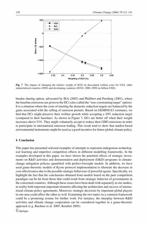
138 Climatic Change (2006) 79:121–141
Fig. 7 The impact of changing the relative weight of SUD on discounted welfare costs for USA, otherindustrialized countries (IND) and developing countries (SUD), 2000–2050 (in billion USD).
burden sharing option, advocated by IEA (2002) and Philibert and Pershing (2001), wherethe baseline emissions are given to the DCs (also called the “non-constraining target” option).It is a situation where the costs of meeting the domestic reduction targets are balanced by thegains associated with the selling of emission permits. Based on GEMINI-E3 estimates, wefind that DCs might preserve their welfare growth while accepting a 20% reduction target(compared to their baseline). As shown in Figure 7, DCs are better off when their weightincreases above 53%. They might voluntarily accept to reduce their GHG emissions in orderto participate in international emission trading. This result tend to show that market-basedenvironmental instruments might be used as a good incentive for future global climate policy.
4 Conclusion
This paper has presented selected examples of attempts to represent endogenous technolog-ical learning and imperfect competition effects in different modelling frameworks. In theexamples developed in this paper, we have shown the potential effects of strategic invest-ments on R&D activities and demonstration and deployment (D&D) programs in climate-change mitigation policies quantified with perfect-foresight models. In addition, we haveused game-theoretic models of Kyoto protocol implementation to illustrate the decrease incost-effectiveness due to the possible strategic behaviour of powerful agents. Specifically, wehighlight the fact that the conclusions obtained from models based on the pure competitionparadigm can be far from those that could result from strategic behavior of governments inthe concerned countries. Although these issues have been dealt with separately in our studies,in reality both represent important elements affecting the architecture and success of interna-tional climate-policy agreements. Moreover, strategic decisions by important global playersin one area could affect the other as well. Examining the two topics in a common frameworkcould be a promising avenue for further work. For instance, the interplay between R&Dactivities and climate change cooperation can be considered together in a game-theoreticapproach (e.g. Buchner et al. 2005; Kemfert 2005).
Springer
Climatic Change (2006) 79:121–141 139
The main results of our analysis can be summarized as follows:
– The endogenization of experience curves represents an advance in the modeling of tech-nological change in energy-system models, capturing the early investments required fora technology to progress and achieve long-term cost competitiveness in the marketplace(Messner 1997). Our analysis illustrates the role that early investments on R&D activitiesand demonstration and deployment (D&D) programs could play in supporting the devel-opment and diffusion of cleaner technologies in the long term. Public-private partnershipsand international co-operation on these topics could be useful to share the risks and costs ofclean technology development and diffusion. Our results highlight the importance of thesetwo policy instruments as key strategic elements in climate-change mitigation strategies,which must be designed such that they encourage technological innovation and progressand enable a transition in the long run towards a cleaner, more efficient, and supply securetechnological path.
– As a consequence of the U.S. withdrawal of the Kyoto Protocol, low-cost countries (i.e.Russia) may have a strong incentive for strategic behavior on the CO2 market; however, oursimulations show that this market power will ultimately depend on developing countries’strategies in future commitment periods.
– High-cost countries might be tempted to act strategically in climate policy implementation,and to favor their domestic industry through the initial allocation of emissions quotas; whenthe emissions markets are imperfect (i.e. some sectors are excluded from the EU emissionstrading system), these non-cooperative behaviors increase the global cost of the carbonconstraint.
– The Post-Kyoto negotiation should focus on the global GHG concentration target to be metcollectively and the implementation of a world emission trading regime; Once countries andregions agree on the coupled long term constraint, developing countries might voluntaryaccept emissions caps that would result from a non-cooperative equilibria in order to sellemission permits.
Acknowledgements This research has been supported by the Swiss NSF under an National Centre of Com-petence in Research on Climate (NCCR-climate) grant.
References
Aumann RJ (1974) Subjectivity and correlation in randomized strategies. Journal of Mathematical Economics1:67–96
Babiker M, Criqui P, Ellerman D, Reilly J, Viguier L (2003) Assessing the impact of carbon tax differentiationin the European Union. Environmental Modeling & Assessment 8(3):187–197
Babiker M, Reilly J, Viguier L (2004) Is international emission trading always beneficial? The Energy Journal25(2):33–56
Basar T, Olsder G (1989) Dynamic noncooperative game theory. Academic Press, LondonBahn O, Kypreos S (2002) MERGE-ETL: An optimisation equilibrium model with two different endogenous
technological learning formulations. PSI Report 02-16, Paul Scherrer Institute, VilligenBarreto L (2001) Technological learning in energy optimisation models and the deployment of emerging
technologies. Thesis no. 14151, Swiss Federal Institute of Technology Zurich (ETHZ)Barreto L, Kypreos S (2004a) Emissions trading and technology deployment in an energy-systems “Bottom-
Up” model with technology learning. European Journal of Operational Research 158:243–261Barreto L, Kypreos S (2004b) Extensions to the Energy-System GMM Model for SAPIENTIA. Report to the
EC-sponsored SAPIENTIA Project ENK6-CT-2002-00614, Paul Scherrer Institute, Energy EconomicsGroup, Paul Scherrer Institute, Villigen, Switzerland
Barrett S (1997) The strategy of trade sanctions in international environmental agreements. Resource andEnergy Economics 19:345–561
Springer
140 Climatic Change (2006) 79:121–141
Barrett S (1999) A theory of full international cooperation. Journal of Theoretical Politics 11(4):519–41Bernard A, Haurie A, Vielle M, Viguier L (2005) A two-level dynamic game of carbon emissions trading
between Russia, China, and Annex B Countries. Journal of Economic Dynamic & Control. PreliminaryAccepted for Publication
Bernard A, Paltsev S, Reilly J, Vielle M, Viguier L (2003) Russia’s role in the Kyoto Protocol. Report 98,MIT Joint Program on the Science and Policy of Global Change, Cambridge MA
Bernard A, Vielle M (1998) La structure du modele GEMINI-E3. Economie & Prevision 5(136)Bernard A, Vielle M (2003) Measuring the welfare cost of climate change policies: A comparative assessment
based on the computable general equilibrium model GEMINI-E3. Environmental Modeling & Assessment8(3):199–217
Buchner B, Carraro C, Cersosimo I, Marchiori C (2005) Back to Kyoto? US participation and the linkagebetween R&D and climate cooperation. In: Haurie A, Viguier L (eds) Cloupling climate and economicdynamics. Kluwer Academic Publishers, Chapt. 5
Carraro C, Siniscalco D (1996) R&D cooperation and the stability of international environmental agreements,In: Carraro C (ed) International environmental negotiations. Kluwer Academic Publishers
Ciscar J, Soria A (2004) Kyoto and beyond Kyoto climate policy: comparison of open-loop and feedbackgame outcomes. In: Carraro C, Fragnelli V (eds) Game practice and the environment. Cheltenham, UK-Northampton, MA: Edward Elgar
Criqui P (1996) POLES 2.2, Technical Report, JOULE II Programme, European Commission DG XVII -Science Research Development, Bruxelles, Belgium
Criqui P, Viguier L (2000) Kyoto and technology at world level: Costs of CO2 reduction under flexibilitymechanisms and technical progress. International Journal of Global Energy Issues 14:155–168
Dockner E, Jorgensen S, Long N, Sorger G (2000) Differential games in economics and management sciences.Cambridge, UK: Cambridge University Press
EC (2002) Communication from the commission on impact assessment. Technical Report COM(2002) 276Final, European Commission, Brussels, Belgium
Fishbone L, Abilock H (1981) MARKAL, a linear programming model for energy systems analysis: technicaldescription of the BNL version. International Journal of Energy Research 5:353–375
Forgo F, Fulop J, Prill M (2005) Game theoretic models for climate change negotiations. European Journal ofOperational Research 160:252–267
Germain M, Toint P, Tulkens H, de Zeew A (1998) Transfers to sustain core-theoretic cooperation in interna-tional stock pollutant control. Discussion Paper 9832, CORE
Goulder L, Mathai K (2000) Optimal CO2 abatement in the presence of induced technological change. Journalof Environmental Economics and Management 39:1–38
Hahn R (1984) Market power and transferable property rights. Quarterly Journal of Economics 99(4):753–765
Haurie A, Moresino F, Vielle M, Viguier L (2005a) A coupled equilibrium model of international climatepolicy. Mimeo
Haurie A, Moresino F, Viguier L (2005b) A two-level differential game of international emissions trading.Annals of the International Society of Dynamic Games. To appear
Haurie A, Viguier L (2003) A stochastic dynamic game of carbon emissions trading. Environmental Modelingand Assessment 8:239–248
IEA (2002) Beyond Kyoto. Energy dynamics and climate stabilisation. Paris, France: International EnergyAgency
Kemfert C (2005) Climate policy cooperation games between developed and developing nations: a quantita-tive, applied analysis. In: Haurie A, Viguier L (eds) Cloupling climate and economic dynamics. KluwerAcademic Publishers, Chapt. 5
Kouvaritakis N, Soria A, Isoard S (2000) Modelling energy technology dynamics: methodology for adaptiveexpectations models with learning by doing and learning by searching. Int. J. of Global Energy Issues14(1/2/3/4):104–115
Kypreos S (2000) The MERGE model with endogenous technological change. In: Proceedings of the economicmodeling of environmental policy and endogenous technological change workshop. Amsterdam, TheNetherlands, pp. 16–17
Kypreos S (2005) Modeling experience curves in MERGE. Energy 30(14):2721–2737Kypreos S, Bahn O (2002) A MERGE model with endogenous technological change. Environmental Modeling
and Assessment 8:249–259Loulou R, Lavigne D (1996) MARKAL model with elastic demands: application to GHG emission con-
trol, In: Carraro C, Haurie A (eds) Operations research and environmental management. Vol. 5 of TheFEEM/KLUWER International series on economics, energy and environment. Kluwer Academic Pub-lishers, pp. 201–220
Springer

Climatic Change (2006) 79:121–141 141
Manne A, Barreto L (2004) Learn-by-doing and carbon dioxide abatement. Energy Economics 26:621–633Manne A, Richels R (2001) An alternative approach to establishing trade-offs among greenhouse gases. Nature
401:675–677Manne A, Richels R (2002) The impact of learning-by-doing on the timing and costs of CO2 abatement. In:
International Energy Workshop. Stanford, USA, pp. 18–20Messner S (1997) Endogenised technological learning in an energy systems model. Journal of Evolutionary
Economics 7:291–313Philibert C, Pershing J (2001) Considering the options: Climate targets for all countries. Climate Policy
1:211–227Rafaj P, Kypreos S, Barreto L (2005) Flexible carbon mitigation policies: analysis with a global multi-regional
MARKAL model. In: Haurie A Viguier L (eds) Cloupling climate and economic dynamics. KluwerAcademic Publishers, Chapt. 5
Rosen JB (1965) Existence and uniqueness of equilibrium points for concave N -person games. Econometrica33(3):520–534
Stavins R (1995) Transaction costs and tradable permits. Journal of Environmental Economics and Manage-ment 29:133–48
Viguier L, Vielle M, Haurie A, Bernard A (2006) A two-level computable equilibrium model to assess thestrategic allocation of emission allowances within the european union. Computers & Operations Research33(2):369–385
Springer
Climatic Change (2006) 79:143–162DOI 10.1007/s10584-006-9147-x
Economics of climate policy and collectivedecision making
Beat Burgenmeier · Andrea Baranzini ·Catherine Ferrier · Celine Germond-Duret ·Karin Ingold · Sylvain Perret · Peter Rafaj ·Socrates Kypreos · Alexander Wokaun
Received: 10 November 2004 / Accepted: 13 April 2006 / Published online: 8 November 2006C© Springer Science + Business Media B.V. 2006
Abstract This paper explores the reasons why economic instruments of climate change arereluctantly applied and stresses the need for interdisciplinary research linking economic the-ory and empirical testing to deliberative political procedures. It is divided in three parts. Thefirst one recalls the main issues in implementing Cost-Benefit Analysis such as informationproblems, uncertainties, discounting the future and irreversibilities. The second part showshow these issues can be treated in integrated assessment and techno-economic models andpresents a case study, which shows that
� The chosen scenario tends to stabilize atmospheric CO2 concentration at around 550 ppmin the long run.
� Exclusion of possibility to trade CO2 emission permits under a cap regime would increasethe cost of emission abatement for OECD countries.
� Combining different flexibility instruments might lead to significant gains in the overallcost of climate policy.
The third part presents results of a survey conducted among the main economic andenvironmental associations in Switzerland. The survey reveals conflicting views on economic
B. Burgenmeier (�) · C. Ferrier · K. Ingold · S. PerretCentre of Human Ecology and Environmental Sciences, University of Geneva, 40 Bd du Pont-d’Arve,CH-1211, Geneva, Switzerlande-mail: [email protected]
A. BaranziniGeneva School of Business Administration, University of Applied Sciences of Western Switzerland
C. Germond-DuretGraduate Institute of International Relations, University of Geneva
S. Kypreos · A. WokaunPaul Scherrer Institute
P. RafajInternational Institute for Applied Systems Analysis, Austria
Springer
144 Climatic Change (2006) 79:143–162
instruments. It shows how the social acceptability of these instruments can be improved intaking explicitly into account these opposing views of special interest groups. Therefore,policy scenarios should be selected in combining techno-economic models with empiricalstudies about their political and normative context.
1 Introduction
Climate change calls for a policy response. The Kyoto Protocol explicitly refers to economicinstruments and delegates their application to the ratifying States. However as the OECDnoted, these instruments are theoretically well founded, but badly applied (Barde 1997). Thischapter examines the reasons for this limited success of economic instruments and exploressome conceptual problems and in implementing Cost-Benefit Analysis in a political decisionmaking process. Different policy recommendations face a social acceptance problem indeed(cf. Spash and Carter 2002).
This contribution is divided into three parts. The first one recalls some theoretical aspectsof economic instruments based on cost-benefit analysis (CBA). The second one presents casestudies for greenhouse gas emission control using models of the NCCR project to overcomethe weaknesses related to CBA or the precautionary principle. Based on neoclassical eco-nomic theory and the use of techno-economic models some policy responses are evaluated.Finally, the third part, discusses the social acceptance problem in presenting the result of asurvey conducted among 240 Swiss economic and the nine main environmental associationsthat form the main special interest groups in the implementation process of climate changepolicies. As a way of conclusion, some fundamental issues of economic instruments for cli-mate change policy are discussed as controversies on their implementation are at the root oftheir social acceptance.
2 Issues in implementing cost-benefit and cost effectiveness analysis
The global warming problem can be addressed through five interrelated questions:
i By how much should greenhouse gases (GHGs) emissions be reduced? Answers to thisquestion would help, for instance to assess the reduction targets actually discussed at theinternational level, e.g. in the Kyoto Protocol.
ii When should GHGs emissions be reduced? This issue is related to the timing of emissionsabatement, e.g. is it better to reach a predetermined target relatively fast or is it preferredto wait and benefit from new information and technological advances?
iii How should emissions be reduced? This question is closely associated with the choiceof policy instruments (e.g. regulations, economic instruments, voluntary agreements, andpublic investments) that could be implemented to achieve the required targets.
iv Who should reduce emissions? Responses to this interrogation involve equity consider-ations on, in particular, who has to bear the burden of the costs of climate policies andimpacts.
v At which level should the decision intervene? Though climate change is a global phe-nomenon, actions are needed on all levels of intervention; the link between the interna-tional, national and local levels raises a coordination problem, as different jurisdictionsintervene.
Springer
Climatic Change (2006) 79:143–162 145
The answers to these questions are particularly challenging, because of the peculiarfeatures of the global warming problem, such as large uncertainties, non-linearities andirreversibilities, possible catastrophes with small probabilities, asymmetric distribution ofimpacts, very long planning horizon, changing social perception, and the global and publicgood characteristics of the problem (IPCC 1996).
CBA plays a prominent part in modelling economic decision-making procedures (cf.Nordhaus (1993), Falk and Mendelsohn (1993), and Maddison (1995)). CBA is a decisionsupport technique, which was initially developed for project evaluation. The aim of CBA isto maximise economic efficiency or, in other words, to determine (economically) optimalpolicies. To achieve this, the CBA approach expresses widely different impacts in monetaryterms, usually using market prices (or adjusted market prices, when markets are distorted orwhen the policy implies non-marginal changes). CBA applies a discounting procedure, toaccount for the fact that benefits and costs occur in different points in time.
To evaluate climate policies in a CBA framework, it is then necessary to calculate the ratioof the sum of expected discounted benefits (V) and costs (F) of reducing global warming,Y0 = V0/F0. Where
V0 =T∑
t=0
Bt
(1 + r )t and F0 =T∑
t=0
Ct
(1 + r )t ,
with Bt and Ct the expected benefits and costs at time t, r the appropriate discount rate, andT the time horizon.
The discounted costs are the monetary costs of abatement policies, while discountedbenefits are the level of damage avoidance–the difference between the cost of global warmingin the absence of intervention and the unavoidable costs of global warming associated with agiven abatement policy (which cannot be avoided because greenhouse gases are long-lived).
Following the CBA approach, a policy improves economic efficiency if discounted bene-fits are greater than discounted costs (i.e., when Yt = Vt / Ft > 1). When there are alternativeclimate policies, the optimal is the one with the greatest difference among the sum of dis-counted benefits and cost.
2.1 Information problems
To implement the CBA approach, it is thus necessary to know and quantify all the previousparameters, i.e. costs, benefits and the discount rate, as well as their evolution through time.Of course, in the context of global warming, this is an incredibly complex task and it has toovercome an extraordinary information problem. Moreover, if global warming in the verylong term will banish life on Earth, then only the costs to avoid this outcome have to beaccounted for Benefits derived from human activities will disappear too.
The evaluation of costs of climate policies is illustrated in the GMM model, which willbe presented in the second part of this chapter. The evaluation of the benefits of climatepolicies, especially in monetary terms, is much more subject to debate and dispute. Indeed,fundamental impacts of climate change are not subject to trading in markets, or are traded invery imperfect and limited markets. For instance, climate change may have impacts on humanhealth and increase mortality and morbidity; may oblige people to migrate from an exposedarea; or may modify ecosystems and reduce biodiversity. The most serious consequencesof those impacts are of course outside the realm of the markets. In the past decade, a largebody of the environmental economics literature developed and applied several techniques
Springer
146 Climatic Change (2006) 79:143–162
to value non-market assets in monetary terms, ranging from human capital techniques anddefensive expenditures approaches to hedonic techniques and contingent valuation methods(e.g. see Cropper 2000). Those techniques are different in their application, but they areall fundamentally based on the same principle: simulate the existence of a market, for anasset, which is not marketed. Those techniques are thus inferring the willingness to pay(willingness to accept a compensation) of individuals for an improvement in environmentalquality (decrease in environmental impacts). This implies that the monetary assessments ofclimate change are strongly conditioned by income and income distribution, which meansthat the value of similar impacts, such as the risks to human life, turns out to be very differentin different countries (see Anaheim 2002).
However, economic valuation techniques are but one step in the complex process for themonetary valuation of the benefits of climate change policies. As E. J. Mishan pointed out: “. . .benefits aggregates, of course, no longer carry any independent economic recommendation.They are value only insofar as they are made use of by the political authority as an inputinto the decision making process, an input to which any weight/including a zero weight) canbe attached” (Mishan 1980, p. 157). Therefore, valuation of the benefits of climate changepolicies is an interdisciplinary endeavour, involving sciences like climatology, epidemiologyand ecology, while economic techniques are then used to express the impacts in monetaryterms, and other social sciences can be implicated to assess their social pertinence. Butexpressing costs and benefits of climate change policies in monetary terms is challenged bythe view that the main aspects of environment evaluation fundamentally escape quantificationand involves beliefs and finally symbolic social representations of nature, which cannot beexpressed in monetary terms (cf. Funtowicz and Rawetz 1994).
2.2 Uncertainties
Monetary valuation will inevitably be faced with fundamental uncertainties. Those uncer-tainties will never be solved, since valuation has to be carried out not only for the present,but also for the future. Indeed, in the future we will not only have different economies, butdifferent individuals and societies, with different preferences and attitudes. According toArrow et al. (1996), those uncertainties may be classified in three areas:
� Scientific uncertainties, which relate e.g. to the relationships between ghg emissions andconcentrations, climate feedbacks, and effects of climate change on temperature and on bio-geo-chemical cycles. The understanding of global climate change and its inter-connexionswith microclimate change is only at its beginnings. This link may be of crucial importancefor implementing climate change on national or regional levels.
� Socio-ecologic uncertainties, concerning the relationships between human societies andnature, e.g. agriculture production and diseases, water use and air pollution.
� Socio-economic uncertainties, which are connected to the effects of climate change onhuman welfare.
2.3 Discounting the future
The final parameter that has to be quantified to apply the CBA approach is the discount rate.The issue of the correct discount rate to be used in CBA is an endless debate in economics,which can be traced back to Ramsey (1928). Ramsey contended that at the public level it isnot ethically defendable to actualise future generations’ welfare (i.e. the discount rate shouldbe nil). In the climate change context, the role of the discount rate is amplified, given the
Springer
Climatic Change (2006) 79:143–162 147
very long planning horizon. Indeed, using a real discount rate of 5 to 10 percent (as used inmany public projects) corresponds to artificially shortening the time horizon. In other words,a relatively high discount rate implies that some of the impacts of climate policies will not beconsidered, when they will occur relatively far into the future (e.g. 50 to 100 years from now).For instance, 1 million damages in 100 years resulting from climate change is worth in presentvalue about 70 if discounted at 10%, about 7’600 discounted at 5% and 370’000 at 1%.
The choice of the discount rate will thus have a decisive impact on the optimality of a givenclimate policy. In fact, given the very long time horizon, climate change strengthens the trade-off concerning the ambivalent role of the discount rate as a mean to reach simultaneously theefficiency in the inter-temporal allocation of resources and inter-generation equity. How canefficiency be separated analytically from equity in order to recommend economic policiesto climate change though in the implementation process both are interrelated? The discountrate, which also refers to the inter-temporal efficiency and equity, can only be analysed withreference to the social objective function (cf. Burgenmeier 2003). For the latter, it meansthat it is necessary to consider the ethical foundations of maximising the sum of discountednet benefits as the social objective (of climate change policies). Indeed, maximising thesum of discounted net benefits (which corresponds to the CBA Social objective) does notprevent decreasing net benefits for some generations, which may be in contrast with theconcept of sustainable development where the common denominator is an ethical claim ofintergenerational equity.
For the inter-temporal efficiency aspects, the discount rate should reflect the opportunitycosts of future social net benefits (benefits minus costs) resulting from a given policy. At theindividual level, the discount rate is likely to be greater than zero, if capital is productiveand if individuals have a preference for the present vs. the future. It can be shown that theindividual discount rate of consumption (rc) is equal to (cf. Hanley 1992): rc = ρ + ε(c) c
c ,with ρ the individual “pure” time preference (due to impatience, the limited duration of lifeand uncertainty) and ε(c) the elasticity of the utility of consumption. Thus, even if the puretime preference is nil, the individual discount rate can be positive, if consumption is growing.
If capital markets are perfectly competitive, the interest rate is a good measure of theindividual discount rate. However, in reality capital markets are often distorted. In addition,and more fundamentally, the individual discount rate may be different from the one thatsociety would use to express preferences through time. There are several reasons, which mayjustify that the social discount rate is lower than the individual one. In particular, contrary toindividuals, society has a planning horizon that is infinite, since its expected life is (hopefully)not finite. Moreover, some risks may be spread at the collective level, whereas it is not possibleat the individual level. In their seminal paper Arrow and Lind (1970) have even demonstratedthat if the risk may be perfectly spread, then the community may be considered as risk neutral,even if it composed of risk-averse individuals. In that case, the discount rate should not becorrected (increased) to account for uncertainty.
However, the risks associated with climate change are relatively difficult to spread, in par-ticular those related to catastrophic events. Indeed, those risks may be very high and thus dif-ferent from zero, even when divided among a (finite) number of individuals. In addition, thesekinds of risks possess public good characteristics and thus it cannot be divided between indi-viduals, since uncertainty will nevertheless remain the same for each individual (non-rivalry).
2.4 Uncertainty, irreversibilities and climate catastrophes
As detailed above, uncertainty is an inherent feature of climate change. Moreover, the effectsof uncertainty on optimal abatement policies are amplified by irreversibility. In the literature,
Springer
148 Climatic Change (2006) 79:143–162
irreversibility possesses two forms (see Goldemberg et al. 1996). A decision may be consid-ered as irreversible when it reduces future possibilities of choice for a long period of time(Henry 1974).
The first is the irreversibility of climate change: once GHG emissions go into the at-mosphere, they can only be removed naturally, but the rate of decay is extremely low, inparticular for CO2. The second is capital irreversibility: to control ghg emissions, significantinvestments could be involved, and once made, they cannot be undone quickly.
The possibility of catastrophic events is also a main feature of global warming. Indeed, cli-mate change could be a gradual and slow process, but some of its impacts may occur abruptlyor over a short period of time, as some climatological parameters cross threshold values (Na-tional Research Council 2002). Examples of sudden global warming catastrophes are:
(i) The “runaway” greenhouse effect (climate change is much greater and occurs muchfaster than the common consensus indicates);
(ii) Disintegration of the West Antarctic Ice Sheet;(iii) Structural changes in ocean currents (which may lead to a sharp drop in European mean
temperatures).
The first studies applying CBA to determine optimal climate policies did not address theseimportant features, but there is now a substantial literature, which extends traditional CBAto account for uncertainty and irreversibility in the global warming context. However, only afew authors have attempted to include the possibility of catastrophic events (c.g. Baranzini etal. (2003), who show that (i) gradual, continuous uncertainty in the global warming processis likely to delay the adoption of optimal abatement policies, with respect to the standardCBA; but (ii) the possibility of climate catastrophes accelerates the implementation of thesepolicies as their net discounted benefits increase significantly).
3 CBA in integrated assessment and techno-economic models
Having in mind the fundamental critique of CBA for setting climate-change policies describedbefore, we operate two models of the NCCR project to address these questions.
First the Integrated Assessment Model (IAM) MERGE is applied in a CBA framework orunder the precautionary principle to describe scenarios that stabilise the carbon concentrationor the maximum temperature change to low levels. MERGE is able to address issues ofuncertainties for key parameters like the climate sensitivity and the ocean diffusivity in astochastic framework where uncertainties will be resolved in the future (Manne and Richels2005).
This IA model can be also extended to address problems of non-linearity and irreversibil-ity or climate catastrophes. For example, the MERGE-E version (Bahn et al. 2006b) specifiestime constraints on temperature changes and rates of temperature changes such that the ther-mohaline circulation (THC) of the North Atlantic will never be interrupted. Temperature con-straints are estimated with the help of specific climate models (Knutti et al. 2002) concerningthe THC. Examples applying MERGE are given in the same special issue (Bahn et al. 2006a).The report of Bahn et al. describes how a neoclassical economic model like MERGE can belinked with a climate model of intermediate complexity to perform analyses in a CBA or ina cost effectiveness framework.
The second model applied in the NCCR project is the energy systems model GMM(a partial equilibrium bottom-up model) where following the precautionary principle weevaluate different policies and targets that stabilize carbon emissions to 10 GtC/yr by theyear 2050. These case studies are imposed as a set of policy overlays on a Baseline sce-
Springer
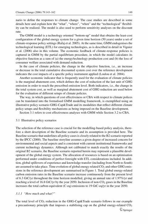
Climatic Change (2006) 79:143–162 149
nario to define the responses to climate change. The case studies are described in somedetails here and explain how the “what”, “where”, “when” and the “technological” flexibil-ity can be realized. The model is also used to perform sensitivity analyses on the discountrate.
The GMM model is a technology oriented “bottom-up” model that obtains the least-costconfiguration of the global energy system for a given time horizon (50 years) under a set ofclimate-response policy settings (Rafaj et al. 2005). At the same time, GMM endogenises thetechnological learning (ETL) for emerging technologies, as is described in detail in Viguieret al. (2006) also in this volume. The economic feedback of climate-response policies iscaptured in GMM by the partial equilibrium procedure, in which the model calculates itsobjective function as a sum of (a) the energy/technology production cost and (b) the loss ofconsumer welfare associated with demand reduction.
In the case of climate policies, the change in the objective function, i.e., an increaseor decrease in the total cumulative discounted system cost over the reference developmentindicates the cost impacts of a specific policy instrument applied (Loulou et al. 2004).
Another economic indicator that is frequently used for the evaluation of climate policiesis the marginal abatement cost, which defines the cost of reduction of the last unit of GHGemission in order to reach the prescribed emission level. Both indicators, i.e., the change inthe total system cost, as well as marginal abatement cost of GHG reduction are used belowfor the evaluation of different setups of climate policies.
The way, in which questions of cost effectiveness or CBA with respect to climate policescan be translated into the formalised GMM modelling framework, is exemplified using anillustrative policy scenario GHG-Cap&Trade and its modalities that reflect different climatepolicy setups and flexibility mechanisms as being imposed on the Baseline development.
Section 3.1 refers to cost effectiveness analyses with GMM while Section 3.2 to CBA.
3.1 Illustrative policy scenarios
The selection of the reference case is crucial for the modelling-based policy analysis, there-fore a short description of the Baseline scenario and its assumption is provided here. TheBaseline scenario that underlines all policy cases is closely related to the B2 scenario reportedby the IPCC (2000). The baseline storyline assumes a given degree of increased concern forenvironmental and social aspects and is consistent with current institutional frameworks andcurrent technology dynamics. Although not calibrated to match exactly the results of theoriginal B2 scenario, the Baseline scenario reported herein may represent a plausible devel-opment of the global energy system. The allocation of resources is based on an optimisationperformed under conditions of perfect foresight with ETL considerations included. In addi-tion, global spillovers of experience and knowledge transfer (including from North to South)are assumed to take place. Time evolution of global energy related CO2 and other GHG emis-sions in the reference development are summarised in Figure 1. Total global energy-relatedcarbon emission rates in the Baseline scenario increase continuously from the present levelof 6.3 GtC/yr throughout the time horizon modelled, giving an annual rate of 1.97%/yr andreaching a level of 16.8 GtC/yr by the year 2050. Inclusion of non-CO2 gases in the Baselineincreases the total carbon-equivalent (C-eq) emissions to 19 GtC-eq/yr in the year 2050.
3.1.1 “How much and what?”
The total level of CO2 reduction in the GHG-Cap&Trade scenario follows in our examplea precautionary principle that imposes a stabilising cap on the global energy-related CO2
Springer
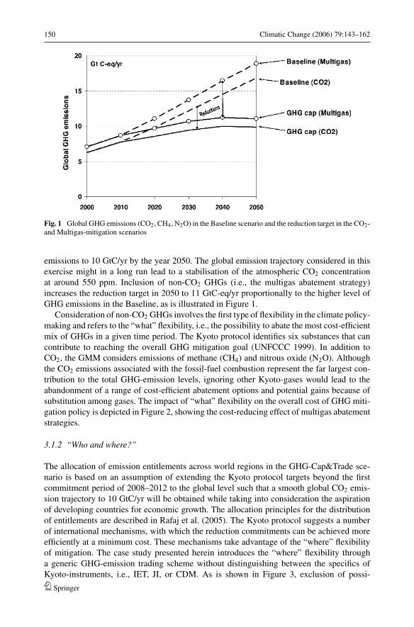
150 Climatic Change (2006) 79:143–162
Fig. 1 Global GHG emissions (CO2, CH4, N2O) in the Baseline scenario and the reduction target in the CO2-and Multigas-mitigation scenarios
emissions to 10 GtC/yr by the year 2050. The global emission trajectory considered in thisexercise might in a long run lead to a stabilisation of the atmospheric CO2 concentrationat around 550 ppm. Inclusion of non-CO2 GHGs (i.e., the multigas abatement strategy)increases the reduction target in 2050 to 11 GtC-eq/yr proportionally to the higher level ofGHG emissions in the Baseline, as is illustrated in Figure 1.
Consideration of non-CO2 GHGs involves the first type of flexibility in the climate policy-making and refers to the “what” flexibility, i.e., the possibility to abate the most cost-efficientmix of GHGs in a given time period. The Kyoto protocol identifies six substances that cancontribute to reaching the overall GHG mitigation goal (UNFCCC 1999). In addition toCO2, the GMM considers emissions of methane (CH4) and nitrous oxide (N2O). Althoughthe CO2 emissions associated with the fossil-fuel combustion represent the far largest con-tribution to the total GHG-emission levels, ignoring other Kyoto-gases would lead to theabandonment of a range of cost-efficient abatement options and potential gains because ofsubstitution among gases. The impact of “what” flexibility on the overall cost of GHG miti-gation policy is depicted in Figure 2, showing the cost-reducing effect of multigas abatementstrategies.
3.1.2 “Who and where?”
The allocation of emission entitlements across world regions in the GHG-Cap&Trade sce-nario is based on an assumption of extending the Kyoto protocol targets beyond the firstcommitment period of 2008–2012 to the global level such that a smooth global CO2 emis-sion trajectory to 10 GtC/yr will be obtained while taking into consideration the aspirationof developing countries for economic growth. The allocation principles for the distributionof entitlements are described in Rafaj et al. (2005). The Kyoto protocol suggests a numberof international mechanisms, with which the reduction commitments can be achieved moreefficiently at a minimum cost. These mechanisms take advantage of the “where” flexibilityof mitigation. The case study presented herein introduces the “where” flexibility througha generic GHG-emission trading scheme without distinguishing between the specifics ofKyoto-instruments, i.e., IET, JI, or CDM. As is shown in Figure 3, exclusion of possi-
Springer
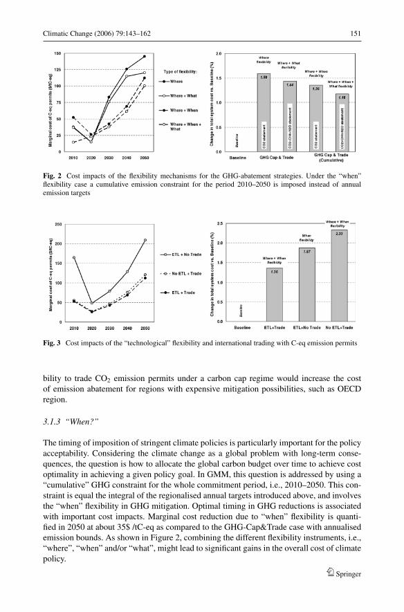
Climatic Change (2006) 79:143–162 151
Fig. 2 Cost impacts of the flexibility mechanisms for the GHG-abatement strategies. Under the “when”flexibility case a cumulative emission constraint for the period 2010–2050 is imposed instead of annualemission targets
Fig. 3 Cost impacts of the “technological” flexibility and international trading with C-eq emission permits
bility to trade CO2 emission permits under a carbon cap regime would increase the costof emission abatement for regions with expensive mitigation possibilities, such as OECDregion.
3.1.3 “When?”
The timing of imposition of stringent climate policies is particularly important for the policyacceptability. Considering the climate change as a global problem with long-term conse-quences, the question is how to allocate the global carbon budget over time to achieve costoptimality in achieving a given policy goal. In GMM, this question is addressed by using a“cumulative” GHG constraint for the whole commitment period, i.e., 2010–2050. This con-straint is equal the integral of the regionalised annual targets introduced above, and involvesthe “when” flexibility in GHG mitigation. Optimal timing in GHG reductions is associatedwith important cost impacts. Marginal cost reduction due to “when” flexibility is quanti-fied in 2050 at about 35$ /tC-eq as compared to the GHG-Cap&Trade case with annualisedemission bounds. As shown in Figure 2, combining the different flexibility instruments, i.e.,“where”, “when” and/or “what”, might lead to significant gains in the overall cost of climatepolicy.
Springer
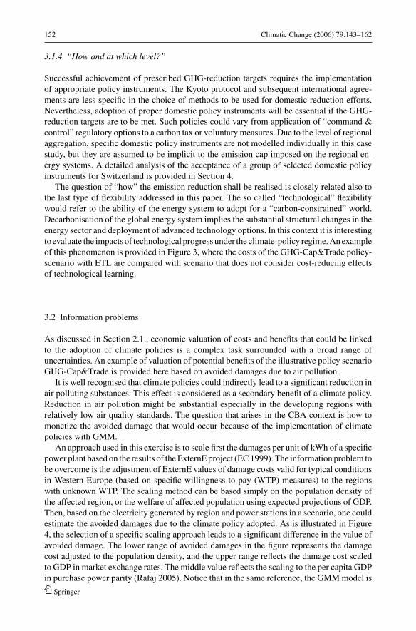
152 Climatic Change (2006) 79:143–162
3.1.4 “How and at which level?”
Successful achievement of prescribed GHG-reduction targets requires the implementationof appropriate policy instruments. The Kyoto protocol and subsequent international agree-ments are less specific in the choice of methods to be used for domestic reduction efforts.Nevertheless, adoption of proper domestic policy instruments will be essential if the GHG-reduction targets are to be met. Such policies could vary from application of “command &control” regulatory options to a carbon tax or voluntary measures. Due to the level of regionalaggregation, specific domestic policy instruments are not modelled individually in this casestudy, but they are assumed to be implicit to the emission cap imposed on the regional en-ergy systems. A detailed analysis of the acceptance of a group of selected domestic policyinstruments for Switzerland is provided in Section 4.
The question of “how” the emission reduction shall be realised is closely related also tothe last type of flexibility addressed in this paper. The so called “technological” flexibilitywould refer to the ability of the energy system to adopt for a “carbon-constrained” world.Decarbonisation of the global energy system implies the substantial structural changes in theenergy sector and deployment of advanced technology options. In this context it is interestingto evaluate the impacts of technological progress under the climate-policy regime. An exampleof this phenomenon is provided in Figure 3, where the costs of the GHG-Cap&Trade policy-scenario with ETL are compared with scenario that does not consider cost-reducing effectsof technological learning.
3.2 Information problems
As discussed in Section 2.1., economic valuation of costs and benefits that could be linkedto the adoption of climate policies is a complex task surrounded with a broad range ofuncertainties. An example of valuation of potential benefits of the illustrative policy scenarioGHG-Cap&Trade is provided here based on avoided damages due to air pollution.
It is well recognised that climate policies could indirectly lead to a significant reduction inair polluting substances. This effect is considered as a secondary benefit of a climate policy.Reduction in air pollution might be substantial especially in the developing regions withrelatively low air quality standards. The question that arises in the CBA context is how tomonetize the avoided damage that would occur because of the implementation of climatepolicies with GMM.
An approach used in this exercise is to scale first the damages per unit of kWh of a specificpower plant based on the results of the ExternE project (EC 1999). The information problem tobe overcome is the adjustment of ExternE values of damage costs valid for typical conditionsin Western Europe (based on specific willingness-to-pay (WTP) measures) to the regionswith unknown WTP. The scaling method can be based simply on the population density ofthe affected region, or the welfare of affected population using expected projections of GDP.Then, based on the electricity generated by region and power stations in a scenario, one couldestimate the avoided damages due to the climate policy adopted. As is illustrated in Figure4, the selection of a specific scaling approach leads to a significant difference in the value ofavoided damage. The lower range of avoided damages in the figure represents the damagecost adjusted to the population density, and the upper range reflects the damage cost scaledto GDP in market exchange rates. The middle value reflects the scaling to the per capita GDPin purchase power parity (Rafaj 2005). Notice that in the same reference, the GMM model is
Springer

Climatic Change (2006) 79:143–162 153
Fig. 4 Comparison of cost and secondary benefits for the GHG-Cap&Trade policy scenario expressed as achange in the cumulative discounted energy system cost relative to the Baseline scenario. (Note: dr = 5%)
used in a more formal CBA framework addressing simultaneously climate policies and theexternal costs associated with electricity generation.
Implications of the modelling results presented in Figure 4 can be highly relevant forpolicy-making efforts in the area of climate change, particularly for the developing countries,since they suggest that the secondary benefits of the CO2-abatement might offset the directcosts of mitigation.
3.3 Discounting issue in the GMM modelling framework
Given the controversy in the proper selection of the discount rate (dr) for climate policiesoutlined in Section 2.3., it is advisable to evaluate the cost impacts using different dr values.A 5% per annum discount rate has been used in the Baseline and policy scenarios reportedabove. Two sensitivity cases are analysed herein for the GHG-Cap&Trade scenario, using thevalues of 3% and 7%. The rate of 3% is indicated by IPCC (2001) as a rate based on “ethical”considerations. The latter value of 7% reflects more the present energy-market situation andthe dr value is used to approximate the cost of capital invested in more risky projects (see,e.g., AEN-NEA 2005).
Figure 5 shows the change in objective function over the Baseline for the GHG-Cap&Tradescenario applying different discount rates of 3, 5, and 7%. For consistency, the cumulativesystem cost in the policy scenarios is compared to the Baseline scenario, calculated by usingthe same discount rates as in the policy cases. Variations in the total discounted cumulativecost relative to the Baseline disclose a decreasing trend in the total cost for the sensitivityscenarios with an increasing dr. The 3%-discounting results in a total cost that is higher thanin the scenarios with dr of 5 and 7%. On the other hand, marginal costs (undiscounted) of C-eqpermits globally traded across world regions are the highest in the case of dr = 7%, whichreflects the increase in the cost of investments in the abatement options needed for reachingthe GHG-reduction target. This trend is pronounced in the second half of the computationalperiod, where the carbon constraint is the most stringent.
3.4 Final thoughts on the policy recommendations based on a modelling exercise
The purpose of the modelling exercise presented in this section was to provide an exampleof how to handle the critical issues raised by CBA as pointed out in Section 2. Clearly, the
Springer
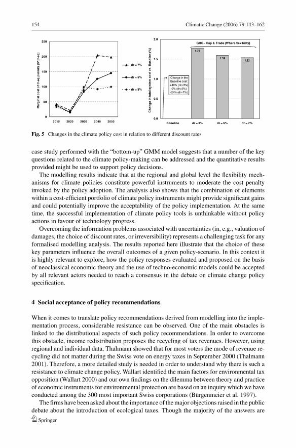
154 Climatic Change (2006) 79:143–162
Fig. 5 Changes in the climate policy cost in relation to different discount rates
case study performed with the “bottom-up” GMM model suggests that a number of the keyquestions related to the climate policy-making can be addressed and the quantitative resultsprovided might be used to support policy decisions.
The modelling results indicate that at the regional and global level the flexibility mech-anisms for climate policies constitute powerful instruments to moderate the cost penaltyinvoked by the policy adoption. The analysis also shows that the combination of elementswithin a cost-efficient portfolio of climate policy instruments might provide significant gainsand could potentially improve the acceptability of the policy implementation. At the sametime, the successful implementation of climate policy tools is unthinkable without policyactions in favour of technology progress.
Overcoming the information problems associated with uncertainties (in, e.g., valuation ofdamages, the choice of discount rates, or irreversibility) represents a challenging task for anyformalised modelling analysis. The results reported here illustrate that the choice of thesekey parameters influence the overall outcomes of a given policy-scenario. In this context itis highly relevant to explore, how the policy responses evaluated and proposed on the basisof neoclassical economic theory and the use of techno-economic models could be acceptedby all relevant actors needed to reach a consensus in the debate on climate change policyspecification.
4 Social acceptance of policy recommendations
When it comes to translate policy recommendations derived from modelling into the imple-mentation process, considerable resistance can be observed. One of the main obstacles islinked to the distributional aspects of such policy recommendations. In order to overcomethis obstacle, income redistribution proposes the recycling of tax revenues. However, usingregional and individual data, Thalmann showed that for most voters the mode of revenue re-cycling did not matter during the Swiss vote on energy taxes in September 2000 (Thalmann2001). Therefore, a more detailed study is needed in order to understand why there is such aresistance to climate change policy. Wallart identified the main factors for environmental taxopposition (Wallart 2000) and our own findings on the dilemma between theory and practiceof economic instruments for environmental protection are based on an inquiry which we haveconducted among the 300 most important Swiss corporations (Burgenmeier et al. 1997).
The firms have been asked about the importance of the major objections raised in the publicdebate about the introduction of ecological taxes. Though the majority of the answers are
Springer
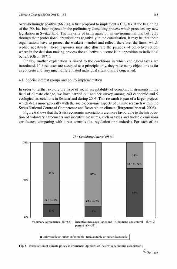
Climatic Change (2006) 79:143–162 155
overwhelmingly positive (66.7%), a first proposal to implement a CO2 tax at the beginningof the ‘90s has been rejected in the preliminary consulting process which precedes any newlegislation in Switzerland. The majority of firms agree on an environmental tax, but replythrough their professional organisations negatively in the consultation. It may be that theseorganisations have to protect the weakest member and reflect, therefore, the firms, whichreplied negatively. These responses may also illustrate the paradox of collective action,where in the decision-making process the collective outcome is in opposition to individualbeliefs (Olson 1971).
Finally, another explanation is linked to the conditions in which ecological taxes areintroduced. If these taxes are accepted as a principle only, they raise many objections as faras concrete and very much differentiated individual situations are concerned.
4.1 Special interest groups and policy implementation
In order to further explore the issue of social acceptability of economic instruments in thefield of climate change, we have carried out another survey among 240 economic and 9ecological associations in Switzerland during 2003. This research is part of a larger project,which deals more generally with the socio-economic aspects of climate research within theSwiss National Centre of Competence and Research on climate (Burgenmeier et al. 2006).
Figure 6 shows that the Swiss economic associations are more favourable to the introduc-tion of voluntary agreements and incentive measures, such as taxes and tradable emissionscertificates, comparing with direct controls (i.e. regulation or standards). For each of the
17% 15%
65%
83% 85%
35%
0%
50%
100%
Voluntary Agreements (N=53) Incentive measures (taxes andpermits) (N=53)
Command and control (N=49)
unfavorable or rather unfavorable favourable or rather favourable
CI = Confidence Interval (95 %)
CI = +/- 9% CI = +/- 9%
CI = +/- 12%
Fig. 6 Introduction of climate policy instruments: Opinions of the Swiss economic associations
Springer
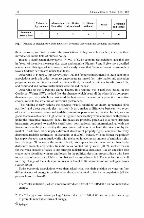
156 Climatic Change (2006) 79:143–162
VoluntaryAgreements
InformationEducation
Certificatesinternational
Certificatesnational
Taxes Commandand control
EconomicAssociations 1 2 3 4 5 6
Fig. 7 Ranking of preferences of forty-nine Swiss economic associations for economic instruments
three measure, we directly asked the associations if they were favorable (or not) to theirintroduction in the field of climate policy.
Indeed, a significant majority (85% +/−9%) of Swiss economic associations state they arein favour of incentive measures (i.e. taxes and permits). Figures 7 and 8 give more detailedresults about this type of instruments and clearly show that Swiss economic stakeholdersfavour tradable certificates rather than taxes.
According to Figure 7, our survey shows that the favourite instruments to these economicassociations are in this order: voluntary agreements are ranked first, information and educationprogrammes second, international certificates third, national certificates fourth, taxes fifth,and command and control instruments were ranked the last.
According to the N-Persons Game Theory, this ranking was established based on theCondorcet Winner (CW) method (i.e. the alternate which beats all the others if on comparesthem even per pair), which is considered the best one so the result of a game (i.e. collectivechoice) reflects the structure of individual preferences.
This ranking clearly reflects the previous results regarding voluntary agreements (firstposition) and direct controls (last position). It also makes a difference between two typesof incentive measures: taxes and tradable emissions permits or certificates. In fact, we canguess that taxes obtained a high score in Figure 6 because they were combined with permitsunder the “incentive measures” label. But taxes are probably perceived as a more stringentinstrument compared to tradable certificates, both national and international as with theformer measure the price is set by the government, whereas in the latter the price is set by themarket. In addition, taxes imply a different structure of property rights, compared to freelydistributed tradable certificates (cf. Baranzini et al. 2000). Indeed, with the former the polluterhas to pay for each ton emitted, while with the latter, it receives an amount of emission rightsfree of charge. Of course, at the emitter’s level, this implies that the tax is costlier than freelydistributed tradable certificates. In addition, as pointed out by Vatter (2002), another reasonfor the weak success of taxes is that stronger redistributive measures (like an emission tax)create more identified winners and losers. In the political decision process, those who haveto pay have often a strong lobby to combat such an amendment bill. The cost factors as wellas every change of the status quo represent a threat to the introduction of ecological taxes(Vatter 2002).
Swiss economic associations were then asked what was their position on votes on fourdifferent kinds of energy taxes that were already submitted to the Swiss population (all theproposals were refused):
1. The “Solar initiative”, which aimed to introduce a tax of Sfr. 0.05/kWh on non renewableenergy,
2. The “Energy conservation package” to introduce a Sfr. 0.03/kWh incentive tax on energyto promote renewable forms of energy,
Springer
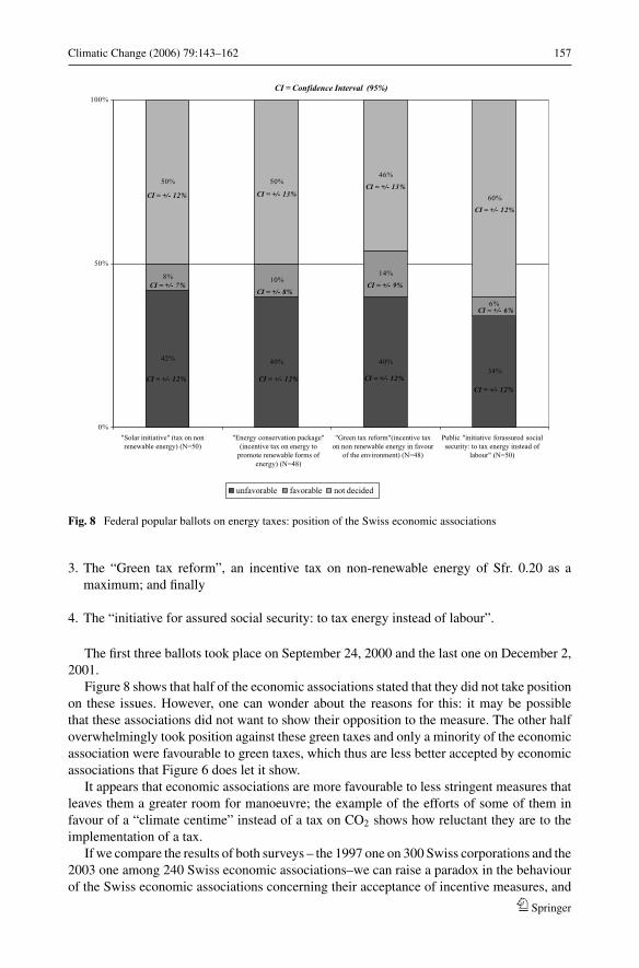
Climatic Change (2006) 79:143–162 157
42% 40% 40%34%
8% 10%14%
50% 50%46%
60%
6%
0%
50%
100%
"Solar initiative" (tax on nonrenewable energy) (N=50)
"Energy conservation package"(incentive tax on energy to
promote renewable forms ofenergy) (N=48)
"Green tax reform"(incentive taxon non renewable energy in favour
of the environment) (N=48)
Public "initiative forassured socialsecurity: to tax energy instead of
labour" (N=50)
unfavorable favorable not decided
CI = +/- 12% CI = +/- 13%
CI = +/- 12%
CI = +/- 7%CI = +/- 8%
CI = +/- 12% CI = +/- 12%
CI = +/- 9%
CI = +/- 13%
CI = +/- 12%
CI = +/- 6%
CI = +/- 12%
CI = Confidence Interval (95%)
Fig. 8 Federal popular ballots on energy taxes: position of the Swiss economic associations
3. The “Green tax reform”, an incentive tax on non-renewable energy of Sfr. 0.20 as amaximum; and finally
4. The “initiative for assured social security: to tax energy instead of labour”.
The first three ballots took place on September 24, 2000 and the last one on December 2,2001.
Figure 8 shows that half of the economic associations stated that they did not take positionon these issues. However, one can wonder about the reasons for this: it may be possiblethat these associations did not want to show their opposition to the measure. The other halfoverwhelmingly took position against these green taxes and only a minority of the economicassociation were favourable to green taxes, which thus are less better accepted by economicassociations that Figure 6 does let it show.
It appears that economic associations are more favourable to less stringent measures thatleaves them a greater room for manoeuvre; the example of the efforts of some of them infavour of a “climate centime” instead of a tax on CO2 shows how reluctant they are to theimplementation of a tax.
If we compare the results of both surveys – the 1997 one on 300 Swiss corporations and the2003 one among 240 Swiss economic associations–we can raise a paradox in the behaviourof the Swiss economic associations concerning their acceptance of incentive measures, and
Springer
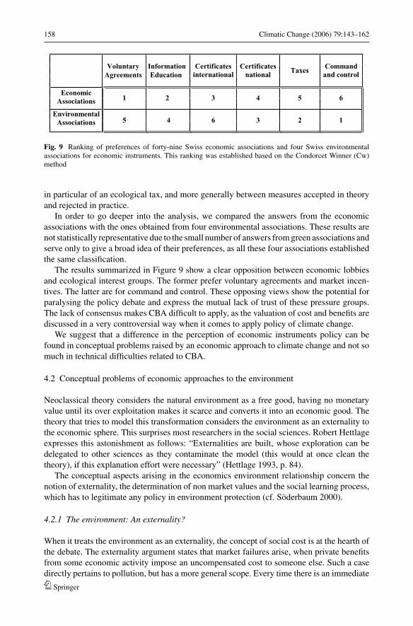
158 Climatic Change (2006) 79:143–162
VoluntaryAgreements
InformationEducation
Certificatesinternational
Certificatesnational
Taxes Commandand control
EconomicAssociations 1 2 3 4 5 6
EnvironmentalAssociations 5 4 6 3 2 1
Fig. 9 Ranking of preferences of forty-nine Swiss economic associations and four Swiss environmentalassociations for economic instruments. This ranking was established based on the Condorcet Winner (Cw)method
in particular of an ecological tax, and more generally between measures accepted in theoryand rejected in practice.
In order to go deeper into the analysis, we compared the answers from the economicassociations with the ones obtained from four environmental associations. These results arenot statistically representative due to the small number of answers from green associations andserve only to give a broad idea of their preferences, as all these four associations establishedthe same classification.
The results summarized in Figure 9 show a clear opposition between economic lobbiesand ecological interest groups. The former prefer voluntary agreements and market incen-tives. The latter are for command and control. These opposing views show the potential forparalysing the policy debate and express the mutual lack of trust of these pressure groups.The lack of consensus makes CBA difficult to apply, as the valuation of cost and benefits arediscussed in a very controversial way when it comes to apply policy of climate change.
We suggest that a difference in the perception of economic instruments policy can befound in conceptual problems raised by an economic approach to climate change and not somuch in technical difficulties related to CBA.
4.2 Conceptual problems of economic approaches to the environment
Neoclassical theory considers the natural environment as a free good, having no monetaryvalue until its over exploitation makes it scarce and converts it into an economic good. Thetheory that tries to model this transformation considers the environment as an externality tothe economic sphere. This surprises most researchers in the social sciences. Robert Hettlageexpresses this astonishment as follows: “Externalities are built, whose exploration can bedelegated to other sciences as they contaminate the model (this would at once clean thetheory), if this explanation effort were necessary” (Hettlage 1993, p. 84).
The conceptual aspects arising in the economics environment relationship concern thenotion of externality, the determination of non market values and the social learning process,which has to legitimate any policy in environment protection (cf. Soderbaum 2000).
4.2.1 The environment: An externality?
When it treats the environment as an externality, the concept of social cost is at the hearth ofthe debate. The externality argument states that market failures arise, when private benefitsfrom some economic activity impose an uncompensated cost to someone else. Such a casedirectly pertains to pollution, but has a more general scope. Every time there is an immediate
Springer
Climatic Change (2006) 79:143–162 159
benefit from an economic activity whose marginal cost is less than the expected marginalrevenue because a third party bears part of the total costs, we are confronted with marketfailure. No incentive to reduce or to stop such an activity exists. The total cost to society isgreater than the cost borne by the one who receives the private benefit. This situation callsfor government intervention. The recommended policy is to ask the government to invoicethe individual for the social cost created, for example through a CO2 tax. This method ofjustifying government intervention consistent with market rules raises a daunting question: towhat degree can the private marginal cost be compared to the social one? Such a comparisonwould only be conceptually acceptable if the costs could be measured objectively (Buchanan1969).
If pollution reduces this value and requires a tax to be introduced, it is followed by incometransfers, which ultimately cannot be evaluated without value judgements.
4.2.2 Non-market values
The value of the natural environment as determined by a market refers to an economic use ofit. Yet the value of the environment is also determined outside the market and independentlyof any economic use. Because the natural environment has an intrinsic value, the marketcannot exclusively determine its worth. Likewise, failure to subject the natural environmentto economic use–albeit possible on both a technological and a normative plane–can give theenvironment a “non-use” value that economists readily associate with an opportunity cost.This cost is part of every economic choice, and is defined by the fact that any economic de-cision related to managing scarce productive resources necessarily implies giving somethingup (cf. Fankhauser 1995).
Climate change policy essentially finds its legitimacy in the change of non-market valuesdetermined by its social perception. This change takes place over a long time, and is codifiedin laws, regulations, morals and customs, which reflect the fact that people are increasinglyaware of problems related to the protection of the environment, despite the fact that theintensity of this awareness can vary. Social concern about an undamaged environment canbe supplanted by other, temporarily more worrying problems such as unemployment.
It is therefore illusory to think that changing social perceptions of the natural environmentwill only change the institutions of a society and leave its perceptions of the economyuntouched. Accordingly, we cannot observe constant and inalterable economic behaviour,but rather a permanent interaction between social values and human behaviour. The originof changing motivations in individual as well as collective behaviour thus becomes crucialto the building of an operational climate change policy.
However, there is no scientific criterion that enables us to move from an individual to acollective level. Society’s economic welfare cannot be defined by simply adding up individualbehaviours, and then treated as a simple problem of factor allocation. A change in the socialutility function does not take into account of the factors, which induced it (Feldman 1983).
4.2.3 Environment protection: A social learning process
In practice, cost-benefit analysis assumes away those factors and relies on engineering ex-pertise. Even if, due to the complexity of the criteria used, impact assessments are made byteams, which also include social scientists, most analyses use a multi-criteria approach, wherethe weighting of the different explanatory factors becomes essential. Engineers apparentlyprefer the weighted sum approach, which does not differentiate between explanatory factorson a qualitative level. Thus, if one variable is considered less important, the low weighting
Springer
160 Climatic Change (2006) 79:143–162
assigned to it cannot do justice to cases where this variable – for example above a certainemission level and sometimes only in relation to another variable – can, during the valuationprocedure, take on a totally different meaning.
A learning aspect not only makes it likely that the value function of the criteria will bechanged, but also increases the information of the actors concerned by the project and theirknowledge of possible interactions between different variables. Consequently, we encountera problem that has become familiar by now, namely the estimation of the social values andcosts submitted to normative judgements, which varies according to the changing socialperception of climate change over time. In other words, taking the related costs into accountis a normative process, dependent on a politico-legal context, which is also supposed to reflectthese changes. This conclusion thus rules out any allegedly objective valuation method.
Recent developments try to weight the different criteria by a normalize approach involvingnon-scientists in the assessment effort (for a survey of the issues and methods used in thisfield, see Rotmans and van Asselt 2002). Therefore, the actors’ information improve duringthe negotiation. The normative dimension of policy recommendations becomes part of theanalysis. As our survey has shown, economic actors such as special interest groups stressthat any assessment must be combined with a negotiation process. They expect increasedtransparency in applying valuation criteria, as well as a learning effect for all the partnersconcerned by a policy recommendation, in order to improve the instruments that are to beintroduced with a view to enhancing climate change.
5 Conclusion: Towards a socially accepted policy mix
The debate about values, the internalisation of social costs and the explicit recognition ofethical aspects make a single minded, exclusive economic approach to climate change policyobsolete. Such an approach contributes to the problems of the social acceptance of economicinstruments. In order to overcome this obstacle the following two interrelated research strate-gies are followed:
� The first research strategy consists of conventional models, that take the environment intoaccount, either through public goods theory or through property rights theory. These twotheories cover the main issues in environmental economics.
� The second strategy refers to more global models, which try to feature relationships betweeneconomics and the biosphere. In the same way, models, which add a social dimension inorder to come closer to the concept of sustainable development (where these three levels:economic, environmental, social are included) also belong to this group, and cover the fieldof ecological economics.
Finally, the crucial point is the integration of the ethical dimension in the traditional the-oretical representations of the economy that society has adopted (Burgenmeier 1993). Thetrend is to delegate ethical questions to the human sciences and thereby to “clean” the eco-nomic model, which then constitutes the main reference. Ethics, as well as the environment,are then being treated as an externality to the market. This distinction makes it possible towork on a “scientific” level and root criteria in a positive sense. Theology and moral phi-losophy are assigned the task of maintaining the social representation of the workings ofthe economy as intact as possible, treating these aspects outside the economic sphere. Theintellectual challenge lies not only in preventing such a development (which is already wellunder way if one is to judge by the many institutes specialised in economical ethics), butalso in integrating ethical considerations in economic reasoning itself (Harsani 1955). The
Springer
Climatic Change (2006) 79:143–162 161
promotion of economic policies of climate change has to be completed by social policiesin order to catch such ethical aspects (Spash 2002). Such social policies not only includetransfers of income, but also basic values of the institutional setting of the market, such aslegal regulation of “fairness” and non-discriminatory practices. This extension inevitablyexposes economics to a dilemma.
� Economic reasoning tries to reduce pollution at the lowest possible cost. It proposes anoptimisation calculus that equalises the marginal cost with the marginal benefit of anyeconomic activity. If many actors on a market are responsible for a given polluting emission,it recommends a policy reducing these where the marginal costs of doing so are smallest.Following the efficiency criterion, economic reasoning therefore allows for a differentiatedtreatment of actors on a market according to their cost or utility functions.
� On the contrary, moral reasoning, often legally codified, is concerned with equality oftreatment, which originates in a normative judgement (for example, through the collectivememory of a community). This normative judgement may also come out of a politicalprocess. If this process is democratic, it is supposed to express the opinion of a majority.Once economic theory recognises that there may be as many normative judgements as actorson the markets (and as many individual actions), legal reasoning only refers to collectivepreferences. Therefore, implementation of climate change policies is normative by nature.Economic modelling has to be extended to the understanding of a political process.
References
AEN-NEA (Nuclear Energy Agency) (2005) Projected costs of generating electricity – 2005 update. OECD-Nuclear Energy Agency, OECD/IEA. Paris, France
Anaheim HA (2002), Impacts of climate change in monetary terms? Issues for Developing Countries. InBaranzini A, Buergenmeier B (Guest Editors) Climate change: issues and opportunities for developingcountries. Special Issue of the Int J Global Env Issues, November 2002, 2(3/4):223–239
Arrow KJ (1951) Social choice and individual values. Wiley, New YorkArrow KJ, Lind RC (1970) Uncertainty and the evaluation of public investment decisions. Am Econ Rev
60(3):364–378Arrow KJ, Parikh, J, Pillet G (1996) Decision-Making Frameworks for addressing climate change, in IPCC,
cit. below, pp 52–77Bahn O, Drouet L, Edwards N, Haurie A, Kypreos S, Stocker T, Vial J-P (2006a) Optimal economic growth
under climate change threats. Climatic Change, DOI 10.1007/s10584-006-9108-4, this issueBahn O, Edwards N, Knutti R, Stocker TF (2006b) Climate policy preventing an Atlantic thermohaline
collapse. Climatic Change (submitted)Baranzini A, Goldemberg J, Speck S (2000) A future for carbon taxes. Ecol Econ 32(3):395–412Baranzini A, Chesney M, Morisset J (2003) The impact of possible climate catastrophes on global warming
policy. Energy Policy 31(8):691–701Barde JP (1997) Economic instruments for environmental protection: experience in OECD countries. in
applying market-based instruments to environmental policies in China and OECD countries, Paris, OECD,pp 31–58
Buchanan J (1969) Cost and choice, an inquiry in economic theory. Chicago University Press, ChicagoBurgenmeier B (1993) Ethical aspects of environmental protection. In: Vernet JP (ed), Environmental con-
tamination, studies in environmental sciences, no. 55. Amsterdam, Londres, New York, Tokyo: ElsevierBurgenmeier B, Harayama Y, Wallart N (1997), Theorie et pratique des taxes environmentales, Economica,
ParisBurgenmeier B (2003) Modelling equity: a debate about values, in Environment Modelling and Assessment,
No 8, pp. 165–174Burgenmeier B, Ferrier C, Germond-Duret C, Ingold K, Perret S (2006) Acceptation des instruments de
marche dans la politique climatique suisse: enquete aupres des principaux acteurs economiques suisses,forthcoming (see also Perret S (2004) “L’acceptabilite des instruments economiques dans le domaine dela politique climatique en Suisse: resultats preliminaires”, Working Paper, No WP4–25
Springer
162 Climatic Change (2006) 79:143–162
Cropper M (2000) Has economic research answered the needs of environmental policy?. J Environ EconManag 39:328–350
Falk I, Mendelsohn R (1993) The economics of controlling stock pollutants: an efficient strategy for greenhousegases. J Environ Econ Manag 25:76–88
Fankhauser S (1995) Valuing climate change. the economics of the greenhouse. Earthscan, LondonFuntowicz SO, Ravetz JR (1994) The worth of a songbird: ecological economics as a post-normal science.
Ecol Econ 10:197–207Henry C (1974) Investment decisions under uncertainty: the irreversibility effect. Am Econ Rev 64(6):1006–
1012Hettlage R (1993) Okonomie auf dem Weg zur Sozialwissenschaft? Revue Suisse de Sociologie 19(1)Intergovernmental Panel on Climate Change (IPCC) (1996) climate change 1995. economic and social di-
mensions of climate change. contribution of working group iii to the 2nd assessment report of the IPCC.WMO and UNEP, New York, Cambridge (U.K.): Cambridge University Press
Intergovernmental Panel on Climate Change (IPCC) (2000) special report on emission scenarios, a specialreport of the working group iii. of intergovernmental panel on climate change, Cambridge UniversityPress, Cambridge (U.K.)
Intergovernmental Panel on Climate Change (IPCC) (2001) climate change 2001: mitigation. contributionof working group iii to the third assessment report of the intergovernmental panel on climate change,Cambridge University Press
Knutti R, Stocker TF, Joos F, Plattner G-K (2002) Constraints on radiative forcing and future climate changefrom observations and climate model ensembles. Nature 416:719–723
Loulou R, Goldstein G, Noble K (2004). Documentation for the MARKAL family of models. Energy Tech-nology Systems Analysis Programme (ETSAP), October 2004
Maddison D (1995) A cost-benefit analysis of slowing climate change. Energy Policy 23(4/5):337–346Manne AS, Richels RG (2005) Global climate decisions under uncertainty. a paper presented at annual meeting
of the international energy workshop 2005, 5–7 July 2005 at the Pa-lu-lu Plaza Kyoto, Kyoto, JapanMishan EJ (1980) How valid are economic evaluations of allocative changes? J Econ Issues XIV(1):143–161National Research Council (2002), Abrupt climate change: inevitable surprises. The National Academics
Press, Washington, DCNordhaus, WD (1993) Rolling the DICE: an optimal transition path for controlling greenhouse gases. Resou
Energy Econ 15:27–50Olson M (1971) Logic of collective action: public goods and the theory of groups. Harvard Universty Press,
revised edition, Cambridge (Mass.)Rafaj P (2005): Analysis of policies contributing to sustainability of the global energy system using the global
multi-regional MARKAL model (GMM), Ph.D. Thesis, Nr. 16122, ETH Zurich 2005Rafaj P, Kypreos S, Barreto L (2005) Flexible carbon mitigation policies: Analysis with a global multi-
regional MARKAL model. In: Haurie A, Viguier L (eds), Coupling climate and economic dynamics.Kluwer Academic Publishers, Dordrecht, The Netherlands, pp 237–66
Rotmans J, van Asselt MBA (2002) Integrated assessment: current practices and challenges for the future. inAbaza H, Baranzini A (eds) implementing sustainable development. integrated assessment and participa-tory decision-making processes. Edward Elgar, Cheltenham, UK, pp 78–116
Soderbaum P (2000) Ecological economics. Earthcan, LondonSpash CL, Carter C (2001) Environmental valuation in Europe: findings from the concerted action, policy
research brief, No 11, European Commission DG-XII, Cambridge Research for Environment (CRE)Spash CL (2002) Greenhouse economics, value and ethics, Routledge, LondonThalmann, Ph (2001) The public acceptance of green taxes: two million voters express their opinion. NCCR
– WP4 Working Paper 1United Nations Framework Convention on Climate Change (UNFCCC): 1999, The Kyoto protocol to the
convention on climate change, UNFCCC Climate Change Secretariat and UNEP, UNEP/IUC/99/10,Geneva, Switzerland
Vatter A (2002), Erfolgsfaktoren klimapolitischer Abstimmungsvorlagen, Buro VatterViguier L, Barreto L, Haurie A, Kypreos S, Rafaj P (2006) Modelling endogenous learning and imperfect
competition effects in climate change economics. Climatic Change, DOI 10.1007/s10584-006-9070-1,this issue
Wallart N (2000), The political economy of environmental taxes. Edgar Elgar, Cheltenham
Springer