climate change: causes, effects, and solutions
TRANSCRIPT

Climate
Change

This Page Intentionally Left Blank
Climate
Change
Causes, Effects,and Solutions
John T. HardyChair, Department of Environmental SciencesHuxley College of the EnvironmentWestern Washington UniversityBellingham, WashingtonUSA
Copyright 2003 John Wiley & Sons Ltd, The Atrium, Southern Gate, Chichester,West Sussex PO19 8SQ, England
Telephone (+44) 1243 779777
Email (for orders and customer service enquiries): [email protected] our Home Page on www.wileyeurope.com or www.wiley.com
All Rights Reserved. No part of this publication may be reproduced, stored in a retrieval system or transmitted inany form or by any means, electronic, mechanical, photocopying, recording, scanning or otherwise, except under theterms of the Copyright, Designs and Patents Act 1988 or under the terms of a licence issued by the CopyrightLicensing Agency Ltd, 90 Tottenham Court Road, London W1T 4LP, UK, without the permission in writing of thePublisher. Requests to the Publisher should be addressed to the Permissions Department, John Wiley & Sons Ltd,The Atrium, Southern Gate, Chichester, West Sussex PO19 8SQ, England, or emailed to [email protected], orfaxed to (+44) 1243 770620.
This publication is designed to provide accurate and authoritative information in regard to the subject mattercovered. It is sold on the understanding that the Publisher is not engaged in rendering professional services. Ifprofessional advice or other expert assistance is required, the services of a competent professional should be sought.
Other Wiley Editorial Offices
John Wiley & Sons Inc., 111 River Street, Hoboken, NJ 07030, USA
Jossey-Bass, 989 Market Street, San Francisco, CA 94103-1741, USA
Wiley-VCH Verlag GmbH, Boschstr. 12, D-69469 Weinheim, Germany
John Wiley & Sons Australia Ltd, 33 Park Road, Milton, Queensland 4064, Australia
John Wiley & Sons (Asia) Pte Ltd, 2 Clementi Loop #02-01, Jin Xing Distripark, Singapore 129809
John Wiley & Sons Canada Ltd, 22 Worcester Road, Etobicoke, Ontario, Canada M9W 1L1
Wiley also publishes its books in a variety of electronic formats. Some content that appearsin print may not be available in electronic books.
British Library Cataloguing in Publication Data
A catalogue record for this book is available from the British Library
ISBN 0-470-85018-3 (HB)ISBN 0-470-85019-1 (PB)
Typeset in 10.5/13pt Times by Laserwords Private Limited, Chennai, IndiaPrinted and bound in Great Britain by Antony Rowe Ltd, Chippenham, WiltshireThis book is printed on acid-free paper responsibly manufactured from sustainable forestryin which at least two trees are planted for each one used for paper production.
Some images in the original version of this book are not available for inclusion in the eBook.
Contents
Preface, ix
Section I Climate Change – Past, Present, and Future, 1
1 Earth and the Greenhouse Effect, 3Introduction, 3The Greenhouse Effect, 3Large-Scale Heat Redistribution, 8Greenhouse Gases, 11Warming Potentials, 19Summary, 20
2 Past Climate Change: Lessons from History, 23Introduction, 23Past Climate Change – Six Historic Periods, 24Methods of Determining Past Climates and Ecosystems, 29Rapid Climate Change, 34Lessons of Past Climate Change, 35Summary, 36
3 Recent Climate Change: The Earth Responds, 39Introduction, 39Atmospheric Temperatures, 40Water Vapor and Precipitation, 43Clouds and Temperature Ranges, 43Ocean Circulation Patterns, 45Snow and Ice, 46Sea-Level Rise, 48Animal Populations, 49Vegetation, 50Attribution, 51Summary, 52
4 Future Climate Change: The Twenty-First Century and Beyond, 55Introduction, 55Global Climate Models, 56
v
vi CONTENTS
Feedback Loops and Uncertainties, 60Scenario-Based Climate Predictions, 67Regional Climates and Extreme Events, 70The Persistence of a Warmer Earth, 71Summary, 73
Section II Ecological Effects of Climate Change, 75
5 Effects on Freshwater Systems, 77Introduction, 77Surface and Groundwater, 78Drought and Soil Moisture, 86Lake and Stream Biota, 86Human Infrastructure, 89Wetlands, 89The Cryosphere, 89Managing Water, 93Summary, 95
6 Effects on Terrestrial Ecosystems, 99Introduction, 99Geographic Shifts in Terrestrial Habitats, 101Vegetation–Climate Interactions, 107Effects of Disturbances, 108Loss of Biodiversity, 109Implications for Forest Management and Conservation Policy, 112Summary, 114
7 Climate Change and Agriculture, 117Introduction, 117Effects of Agriculture on Climate Change, 118Effects of Climate Change on Agriculture, 120US Agriculture, 121Global Agriculture, 123Summary, 128
8 Climate Change and the Marine Environment, 131Introduction, 131Sea-Level Rise, 132Ocean Currents and Circulation, 135Marine Biogeochemistry, 138Marine Ecosystems, 140Summary, 148
CONTENTS vii
Section III Human Dimensions of Climate Change, 151
9 Impacts on Human Settlement and Infrastructure, 153Introduction, 153Energy, 154Environmental Quality, 158Extreme Climatic Events, 159Human Settlements, 160Infrastructure, 162Summary, 167
10 Effects of Climate Change on Human Health, 171Introduction, 171Direct Effects of Heat Stress, 172Infectious Diseases, 174Air Quality, 179Interactions and Secondary Effects, 181Summary, 181
11 Mitigation: Reducing the Impacts, 187Introduction, 187Capture or Sequester Carbon Emissions, 187Reduce Global Warming or Its Effects by Geoengineering, 188Enhance Natural Carbon Sinks, 190Convert to Carbon-Free and Renewable Energy Technologies, 191Conserve Energy and Use It More Efficiently, 201Adapt to Climate Change, 206Taking Action, 206Summary, 208
12 Policy, Politics, and Economics of Climate Change, 211Introduction, 211International Cooperation – From Montreal to Kyoto, 212Meeting Kyoto Targets, 214Post-Kyoto Developments, 217The Politics of Climate Change, 220Kyoto Without the United States, 221Benefits and Costs of Mitigating Climate Change, 224The Future – What is Needed?, 227Summary, 227
Appendixes
A Units, 231
B Abbreviations and Chemical Symbols, 233

viii CONTENTS
C Websites on Climate Change, 235General, 235Journal Articles and Literature on Climate Change, 236Climate Change Education, 236Websites by Chapter Subject Area, 236Conservation and Environmental Action Groups, 240Industry Groups, 240
Index, 241
Preface
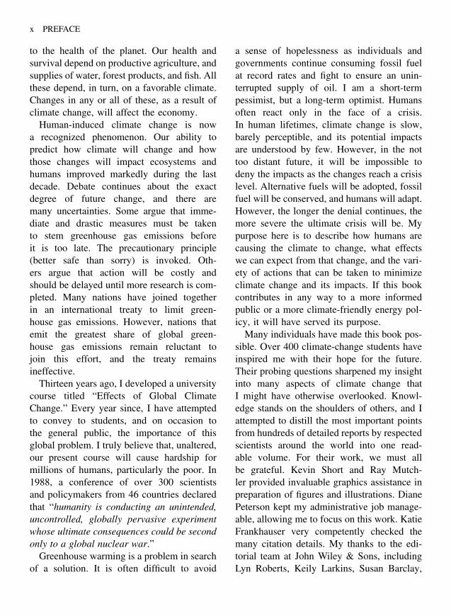
“The greenhouse effect is the most significant economic,political, environmental and human problem facing the 21st Century.”
Timothy Wirth, former US Senator and Undersecretary of State for Global Affairs
Unprecedented changes in climate are tak-ing place. If we continue on our presentcourse, life on Earth will be inextrica-bly altered. The very sustainability of theEarth’s life-support system is now in ques-tion. How did we arrive at this pivotal pointin our history?
For millennia, the Earth’s climate remainedlittle changed. Early humans thrived, living onan abundance of plants and animals, some ofwhich they domesticated for their own use.They cooked their food and warmed theirdwellings largely with wood. This wood wasthe product of photosynthesis – the removalof carbon dioxide from the atmosphere and itsconversion to living organic matter. Burningthe wood returned this same quantity ofcarbon to the atmosphere. Human activitieshad little more than local impacts. Naturalchanges occurred in the Earth’s climate, butthey were gradual, occurring over tens ofthousands to millions of years.
Suddenly, 200 years ago, things began tochange. Modern medicine and improvementsin technology led to a human population
explosion. Ninety-nine percent of all humanbeings who ever lived are alive today. Atthe same time, fossil fuel (first coal, andthen oil and gas) became the energy sourceof choice – facilitating rapid industrializationand further fossil-fuel consumption. Unlikewood, the carbon in fossil fuel was slowlyformed from decaying plants millions of yearsago and was stored in the Earth’s crust. Itsburning over the past 150 years has increasedthe level of atmospheric carbon dioxide by33%. Carbon dioxide is a greenhouse gas thattraps heat in the lower atmosphere, keepingour planet warm. However, like many thingsin nature, a little is good, but more is notnecessarily better.
If we continue our heavy dependence onfossil fuel, we will double the preindustrialatmosphere’s carbon dioxide level in a fewdecades and perhaps triple it by the end of thiscentury. As a consequence, by most estimates,the planet will rapidly warm to a level neverexperienced by human beings. There will beconsequences. In our hurried modern lives, weforget that our welfare is still closely linked
ix
x PREFACE
to the health of the planet. Our health andsurvival depend on productive agriculture, andsupplies of water, forest products, and fish. Allthese depend, in turn, on a favorable climate.Changes in any or all of these, as a result ofclimate change, will affect the economy.
Human-induced climate change is nowa recognized phenomenon. Our ability topredict how climate will change and howthose changes will impact ecosystems andhumans improved markedly during the lastdecade. Debate continues about the exactdegree of future change, and there aremany uncertainties. Some argue that imme-diate and drastic measures must be takento stem greenhouse gas emissions beforeit is too late. The precautionary principle(better safe than sorry) is invoked. Oth-ers argue that action will be costly andshould be delayed until more research is com-pleted. Many nations have joined togetherin an international treaty to limit green-house gas emissions. However, nations thatemit the greatest share of global green-house gas emissions remain reluctant tojoin this effort, and the treaty remainsineffective.
Thirteen years ago, I developed a universitycourse titled “Effects of Global ClimateChange.” Every year since, I have attemptedto convey to students, and on occasion tothe general public, the importance of thisglobal problem. I truly believe that, unaltered,our present course will cause hardship formillions of humans, particularly the poor. In1988, a conference of over 300 scientistsand policymakers from 46 countries declaredthat “humanity is conducting an unintended,uncontrolled, globally pervasive experimentwhose ultimate consequences could be secondonly to a global nuclear war.”
Greenhouse warming is a problem in searchof a solution. It is often difficult to avoid
a sense of hopelessness as individuals andgovernments continue consuming fossil fuelat record rates and fight to ensure an unin-terrupted supply of oil. I am a short-termpessimist, but a long-term optimist. Humansoften react only in the face of a crisis.In human lifetimes, climate change is slow,barely perceptible, and its potential impactsare understood by few. However, in the nottoo distant future, it will be impossible todeny the impacts as the changes reach a crisislevel. Alternative fuels will be adopted, fossilfuel will be conserved, and humans will adapt.However, the longer the denial continues, themore severe the ultimate crisis will be. Mypurpose here is to describe how humans arecausing the climate to change, what effectswe can expect from that change, and the vari-ety of actions that can be taken to minimizeclimate change and its impacts. If this bookcontributes in any way to a more informedpublic or a more climate-friendly energy pol-icy, it will have served its purpose.
Many individuals have made this book pos-sible. Over 400 climate-change students haveinspired me with their hope for the future.Their probing questions sharpened my insightinto many aspects of climate change thatI might have otherwise overlooked. Knowl-edge stands on the shoulders of others, and Iattempted to distill the most important pointsfrom hundreds of detailed reports by respectedscientists around the world into one read-able volume. For their work, we must allbe grateful. Kevin Short and Ray Mutch-ler provided invaluable graphics assistance inpreparation of figures and illustrations. DianePeterson kept my administrative job manage-able, allowing me to focus on this work. KatieFrankhauser very competently checked themany citation details. My thanks to the edi-torial team at John Wiley & Sons, includingLyn Roberts, Keily Larkins, Susan Barclay,

PREFACE xi
and the staff at Laserwords for ably facil-itating the timely completion of this work.I am grateful to my parents who instilledpersistence to see a job to completion. Tomy wife Kathie, my appreciation goes farbeyond the typical author’s appreciation of
patience. Her insightful comments helpedturn a technical treatise into (hopefully) areadable book. Without her inspiration andsupport, none of this would have been writ-ten. Finally, to Kevin, Amy, and Tanya – itsyour planet now.

This Page Intentionally Left Blank

SECTION I
Climate Change – Past, Present,and Future
1

This Page Intentionally Left Blank
Chapter 1
Earth and theGreenhouse Effect
“. . . if the carbonic acid content of the air [atmospheric CO2] rises to 2 [i.e.doubles] the average value of the temperature change will be. . . +5.7 degrees C”
Svante Arrhenius 1896
Introduction
The physics and chemistry of the Earth’satmosphere largely determines our climate(Lockwood 1979). Although the atmosphereseems like a huge reservoir capable of absorb-ing almost limitless quantities of our industrialemissions, it is really only a thin film. Indeed,if the Earth were shrunk to the size of a grape-fruit, its atmosphere would be thinner than theskin of the grapefruit. Our understanding ofhow the chemistry and physics of the atmo-sphere affect climate developed over manycenturies, but has greatly accelerated duringthe past few decades (Box 1.1).
The Earth’s atmosphere is layered. In thelower atmosphere, from the surface up toabout 11-km altitude (troposphere), temper-ature decreases with increasing altitude. Thislayer is only about 1/1,200 of the diameterof the globe, but its physics and chemistryare crucial to sustaining life on the planet.Because cold dense air on top of warm lessdense air is unstable, the layer is fairly turbu-lent and well mixed. It contains 99% of the
atmospheric mass. From 15 to 50 km, the tem-perature increases with altitude, resulting ina stable upper atmosphere (stratosphere) withalmost 1% of the atmospheric mass. Above50 km are the mesosphere and the thermo-sphere, which have little effect on climate(Figure 1.1).
During the past 100 years we humans, as aresult of burning coal, oil, and gas and clear-ing forests, have greatly changed the chemicalcomposition of this thin atmospheric layer.These changes in chemistry, as described insubsequent chapters, have far-reaching con-sequences for the climate of the Earth, theecosystems that are sustained by our climate,and our own human health and economy.
The Greenhouse Effect
Three primary gases make up 99.9% byvolume of the Earth’s atmosphere – nitrogen(78.09%), oxygen (20.95%), and argon(0.93%). However, it is the rare trace gases,that is, carbon dioxide (CO2), methane(CH4), carbon monoxide (CO), nitrogen
Climate Change: Causes, Effects, and Solutions John T. Hardy 2003 John Wiley & Sons, Ltd ISBNs: 0-470-85018-3 (HB); 0-470-85019-1 (PB)
3
4 CLIMATE CHANGE
Box 1.1 The history of atmospheric science
Our current understanding of the chemistry and physics of the atmosphere has a long andfascinating history (Crutzen and Ramanathan 2000). Some highlights of this history includethe following:
340 B.C. – The Greek philosopher Aristotle publishes Meteorologica; its theoriesremain unchallenged for nearly 2000 years.
1686 – Edmond Halley shows that low latitudes receive more solar radiation thanhigher ones and proposes that this heat gradient drives the majoratmospheric circulation.
1750s – Joseph Black identifies CO2 in the air.1781 – Henry Cavendish measures the percentage composition of nitrogen and
oxygen in air.1859 – John Tyndall suggests that water vapor, CO2, and other radiatively active
ingredients could contribute to keeping the Earth warm.1896 – Svante Arrhenius publishes a climate model demonstrating the sensitivity
of surface temperature to atmospheric CO2 levels.1938 – GS Callendar calculates that 150 billion tons of CO2 was added to the
atmosphere during the past half century, increasing the Earth’stemperature by 0.005 ◦C per year during that period.
1920 – Milutin Milankovitch publishes his theory of ice ages based on variationsin the Earth’s orbit.
1957 – Roger Revelle and Hans Suess, renowned oceanographers, proclaim that“human beings are now carrying out a large-scale geophysicalexperiment,” that is, altering the chemistry of the atmosphere withoutknowing the result.
1959 – Explorer Satellites provide images of cloud cover. Verner Suomi estimatesthe global radiation heat budget.
1967 – Syukuro Manabe and Richard Wetherald develop the one-dimensionalradiative-convective atmospheric model and show that a doubling ofatmospheric CO2 can warm the planet about 3 ◦C.
1970–1974 – Destruction of stratospheric ozone by man-made chlorofluorocarbons isdescribed through the work of several researchers.
1985 – The British Antarctic Survey reports a 40% drop in springtimestratospheric ozone between 1956 and 1985.
1986 – Many countries sign the Montreal Protocol on Substances that Deplete theOzone Layer.
1990s – Researchers discover the cooling effect of atmospheric aerosols and theirimportance in offsetting the greenhouse effect. The global warmingtrend continues and record temperatures are repeatedly set.

EARTH AND THE GREENHOUSE EFFECT 5
10−13
10−8
10−3
10−1
1−100 −50 0
Temperature (°C)
Pre
ssur
e (a
tm)
Alti
tude
(km
)
50 100
1000
500
200
100
50
20
10
5
2
1
0
Thermosphere
Mesopause
Stratopause
Tropopause
Troposphere
Mount Everest
Altocumulus cloud
Cumulus cloud
Stratus cloud
Cirrus cloud
Mesosphere
StratosphereOzoneregion
Fig. 1.1 Vertical temperature and pressure structure of the Earth’s atmosphere (From Graedel TE andCrutzen PJ 1997. Atmosphere, Climate, and Change. Scientific American Library, New York:W.H. Freeman and Co, p. 3. Henry Holt & Co.).
oxides (NOx), chlorofluorocarbons (CFCs),and ozone (O3) that have the greatest effecton our climate. Water vapor, with highlyvariable abundance (0.5–4%), also has astrong influence on climate. These trace gasesare known as greenhouse gases or radiativelyimportant trace species (RITS). They areradiatively important because they influencethe radiation balance or net heat balance ofthe Earth.
Thermonuclear reactions taking place on ournearest star, the Sun, produce huge quantities ofradiation that travel through space at the speedof light. This solar radiation includes energydistributed across a wide band of the elec-tromagnetic spectrum from short-wavelengthX rays to medium-wavelength visible light,
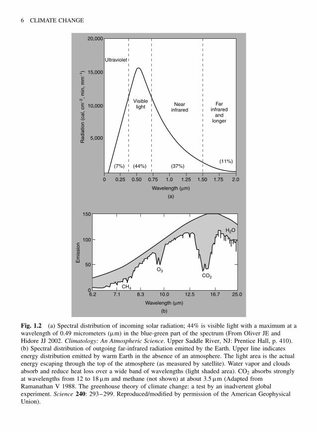
to longer-wavelength infrared. The greatestamount of energy (44%) is in the spectralregion, visible to the human eye from 0.4 (vio-let) to 0.7 µm (red) (Figure 1.2a).
As incoming solar radiation passes throughthe atmosphere, particles and gases absorbenergy. Owing to its physical or chemicalstructure, each particle or gas has specificwavelength regions that transmit energy andother regions that absorb energy. For example,ozone in the stratosphere absorbs short- andmiddle-wavelength ultraviolet radiation. Alarge percentage of incoming solar radiationis in the visible region. Atmospheric watervapor, carbon dioxide, and methane have lowabsorption in this region and allow most ofthe visible light to reach the Earth’s surface.
6 CLIMATE CHANGE
20,000
15,000
10,000
5,000
0.25 0.50 0.75 1.0
Wavelength (µm)
(a)
Rad
iatio
n (c
al, c
m−2
, min
, mm
−1)
1.25 1.50 1.75 2.00
Ultraviolet
Visiblelight
(7%) (44%) (37%)(11%)
Nearinfrared
Farinfrared
andlonger
150
100
50
06.2 7.1 8.3 10.0
Wavelength (µm)
(b)
Em
issi
on
12.5 16.7 25.0
CO2
H2O
CH4
O3
Fig. 1.2 (a) Spectral distribution of incoming solar radiation; 44% is visible light with a maximum at awavelength of 0.49 micrometers (µm) in the blue-green part of the spectrum (From Oliver JE andHidore JJ 2002. Climatology: An Atmospheric Science. Upper Saddle River, NJ: Prentice Hall, p. 410).(b) Spectral distribution of outgoing far-infrared radiation emitted by the Earth. Upper line indicatesenergy distribution emitted by warm Earth in the absence of an atmosphere. The light area is the actualenergy escaping through the top of the atmosphere (as measured by satellite). Water vapor and cloudsabsorb and reduce heat loss over a wide band of wavelengths (light shaded area). CO2 absorbs stronglyat wavelengths from 12 to 18 µm and methane (not shown) at about 3.5 µm (Adapted fromRamanathan V 1988. The greenhouse theory of climate change: a test by an inadvertent globalexperiment. Science 240: 293–299. Reproduced/modified by permission of the American GeophysicalUnion).
EARTH AND THE GREENHOUSE EFFECT 7
After absorption by the Earth’s surface,visible energy is transformed and radiatedback in the far-infrared (heat) region ofthe spectrum at wavelengths greater than1.5 µm (Figure 1.2b). The transparency of theatmosphere to outgoing far-infrared radiation(heat) determines how much heat can escapefrom the Earth back into space and how muchis trapped. The important feature of green-house gases is that they absorb (are opaqueto) certain infrared wavelengths. Water vapor,carbon dioxide, and methane, the same gasesthat transmit visible wavelengths, absorb
strongly in the far infrared (Figure 1.2b).Thus, they trap heat in the troposphere andstop it from escaping to space. Window glassused to trap heat in a greenhouse has similarabsorption and transmission properties; hence,the term “greenhouse gases.”
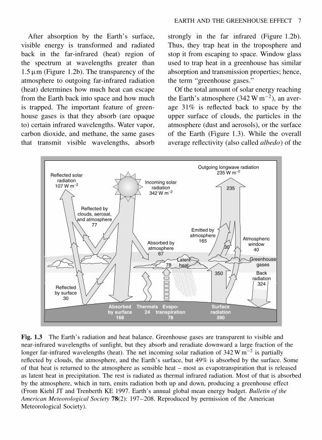
Of the total amount of solar energy reachingthe Earth’s atmosphere (342 W m−2), an aver-age 31% is reflected back to space by theupper surface of clouds, the particles in theatmosphere (dust and aerosols), or the surfaceof the Earth (Figure 1.3). While the overallaverage reflectivity (also called albedo) of the
Reflected solarradiation
107 W m−2 Incoming solarradiation
342 W m−2
Outgoing longwave radiation235 W m−2
Absorbed byatmosphere
67
Emitted byatmosphere
165 Atmosphericwindow
40
Reflected byclouds, aerosal,and atmosphere
77
78Latentheat
30
350
235
Greenhousegases
Backradiation
324Reflectedby surface
30
Absorbedby surface
168
Thermals24
Evapo-transpiration
78
Surfaceradiation
390
Fig. 1.3 The Earth’s radiation and heat balance. Greenhouse gases are transparent to visible andnear-infrared wavelengths of sunlight, but they absorb and reradiate downward a large fraction of thelonger far-infrared wavelengths (heat). The net incoming solar radiation of 342 W m−2 is partiallyreflected by clouds, the atmosphere, and the Earth’s surface, but 49% is absorbed by the surface. Someof that heat is returned to the atmosphere as sensible heat – most as evapotranspiration that is releasedas latent heat in precipitation. The rest is radiated as thermal infrared radiation. Most of that is absorbedby the atmosphere, which in turn, emits radiation both up and down, producing a greenhouse effect(From Kiehl JT and Trenberth KE 1997. Earth’s annual global mean energy budget. Bulletin of theAmerican Meteorological Society 78(2): 197–208. Reproduced by permission of the AmericanMeteorological Society).
8 CLIMATE CHANGE
Earth is 31%, albedo differs greatly betweensurfaces. Clouds, with an albedo of 40 to 90%,are by far the most important reflectors ofincoming solar radiation. The albedo of freshsnow is 75 to 90%, forests 5 to 15%, andthat of water, which depends on the angleof inclination of the Sun, ranges from 2 to>99%. Incoming energy that is not reflected(the remaining 69%) is absorbed by the tro-posphere and the Earth’s surface (Figure 1.3).Evaporation of water requires a considerableamount of energy. This energy is essentiallystored as “latent heat” in water vapor andreleased back into the air as heat when watervapor condenses (Figure 1.3).
Of the total far-infrared (heat) energy rera-diated from the Earth’s surface, 83% is back-radiated and does not directly escape theatmosphere. This back radiation is about dou-ble the amount of energy absorbed by thesurface directly from the Sun. This additionalatmospheric energy warms the Earth to itspresent temperature. Without the greenhousewarming effect of the atmosphere, the Earth’saverage surface temperature would be about−20 ◦C (−4 ◦F) instead of 15 ◦C (59 ◦F). Sim-ply put, greenhouse gases trap solar heat inthe lower atmosphere and keep the Earthwarm. As long as the amount of incomingsolar energy and the amount of greenhousegas in the atmosphere remain fairly constant,the Earth’s temperature remains in balance(Figure 1.3). However, the greater the con-centration of greenhouse gases, the greater theamount of long-wave (heat) radiation trappedin the lower atmosphere.
Large-Scale Heat RedistributionThe Earth’s temperature is not uniformbut differs greatly – geographically (horizon-tally), by elevation (vertically), and over time(seasons and decades). To understand climateand how it might change over decades to cen-turies in the future, we need to understand
Atmosphere
Earth'ssurface Sun
Arctic Circle
Tropic ofCancer
Tropic ofCapricornAntarcticCircle
(a)
(b)
(c)
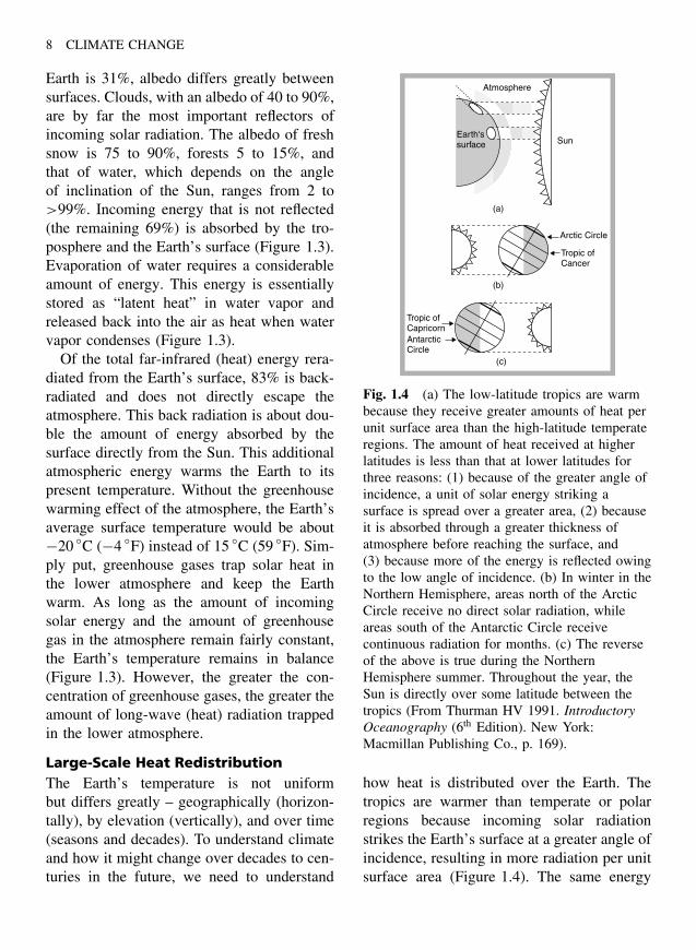
Fig. 1.4 (a) The low-latitude tropics are warmbecause they receive greater amounts of heat perunit surface area than the high-latitude temperateregions. The amount of heat received at higherlatitudes is less than that at lower latitudes forthree reasons: (1) because of the greater angle ofincidence, a unit of solar energy striking asurface is spread over a greater area, (2) becauseit is absorbed through a greater thickness ofatmosphere before reaching the surface, and(3) because more of the energy is reflected owingto the low angle of incidence. (b) In winter in theNorthern Hemisphere, areas north of the ArcticCircle receive no direct solar radiation, whileareas south of the Antarctic Circle receivecontinuous radiation for months. (c) The reverseof the above is true during the NorthernHemisphere summer. Throughout the year, theSun is directly over some latitude between thetropics (From Thurman HV 1991. IntroductoryOceanography (6th Edition). New York:Macmillan Publishing Co., p. 169).
how heat is distributed over the Earth. Thetropics are warmer than temperate or polarregions because incoming solar radiationstrikes the Earth’s surface at a greater angle ofincidence, resulting in more radiation per unitsurface area (Figure 1.4). The same energy
EARTH AND THE GREENHOUSE EFFECT 9
Polar high
60Polarfront
30
0
Equatorial low
SE Trade Winds
High
NE Trade Winds
Westerlies
Polar easterlies
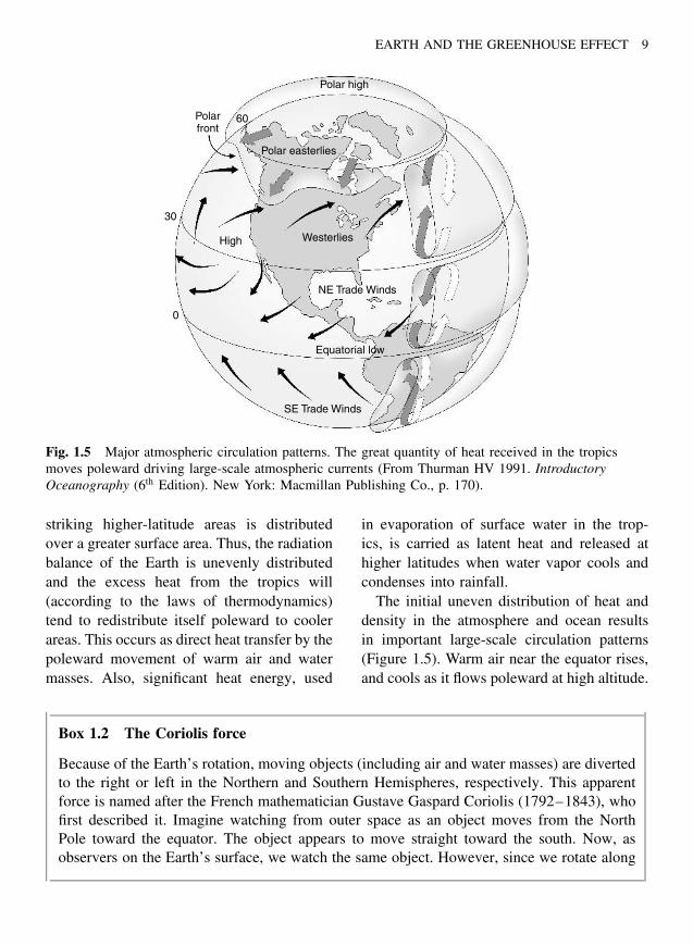
Fig. 1.5 Major atmospheric circulation patterns. The great quantity of heat received in the tropicsmoves poleward driving large-scale atmospheric currents (From Thurman HV 1991. IntroductoryOceanography (6th Edition). New York: Macmillan Publishing Co., p. 170).
striking higher-latitude areas is distributedover a greater surface area. Thus, the radiationbalance of the Earth is unevenly distributedand the excess heat from the tropics will(according to the laws of thermodynamics)tend to redistribute itself poleward to coolerareas. This occurs as direct heat transfer by thepoleward movement of warm air and watermasses. Also, significant heat energy, used
in evaporation of surface water in the trop-ics, is carried as latent heat and released athigher latitudes when water vapor cools andcondenses into rainfall.
The initial uneven distribution of heat anddensity in the atmosphere and ocean resultsin important large-scale circulation patterns(Figure 1.5). Warm air near the equator rises,and cools as it flows poleward at high altitude.
Box 1.2 The Coriolis force
Because of the Earth’s rotation, moving objects (including air and water masses) are divertedto the right or left in the Northern and Southern Hemispheres, respectively. This apparentforce is named after the French mathematician Gustave Gaspard Coriolis (1792–1843), whofirst described it. Imagine watching from outer space as an object moves from the NorthPole toward the equator. The object appears to move straight toward the south. Now, asobservers on the Earth’s surface, we watch the same object. However, since we rotate along
10 CLIMATE CHANGE
with the Earth (in an easterly direction), under the path of the object, it appears to usto veer in a curve toward the right (in a westerly direction), with respect to its directionof movement.
The Coriolis force manifests itself in a number of ways, from riverbanks that erode deeperon one side than the other to winds that rotate counterclockwise around low-pressure areasin the Northern Hemisphere and clockwise in the Southern Hemisphere. The large-scalecirculation of the atmosphere and ocean is strongly affected by the Coriolis force. Usefulgraphical animations of the Coriolis force have been presented by a number of authors (e.g.http://www.windpower.dk or http://satftp.soest.hawaii.edu/ocn620/coriolis/ ).
At about 30◦ latitude, it sinks and flows south-ward again at lower altitudes. To replacethe sinking air mass, air is drawn frompolar latitudes, flows south at high altitudes,sinks, and then flows poleward near the sur-face. These patterns are modified by the
Coriolis force, which pushes the circulationclockwise in the Northern Hemisphere andcounterclockwise in the Southern Hemisphere(Box 1.2). This results in major surface windpatterns at lower altitudes including, forexample, in the Northern Hemisphere, the
Heat transferfrom sea to air
AtlanticOcean
IndianOcean
PacificOcean
Cold, salty, deep current Cold, salty, deep current
Warm, shallow current
Warm, shallow current
Warm
, shallowcurrent
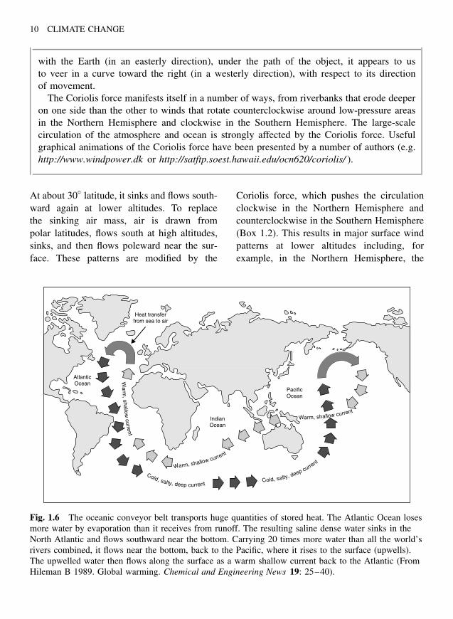
Fig. 1.6 The oceanic conveyor belt transports huge quantities of stored heat. The Atlantic Ocean losesmore water by evaporation than it receives from runoff. The resulting saline dense water sinks in theNorth Atlantic and flows southward near the bottom. Carrying 20 times more water than all the world’srivers combined, it flows near the bottom, back to the Pacific, where it rises to the surface (upwells).The upwelled water then flows along the surface as a warm shallow current back to the Atlantic (FromHileman B 1989. Global warming. Chemical and Engineering News 19: 25–40).
EARTH AND THE GREENHOUSE EFFECT 11
temperate westerly and northeast trade winds(Figure 1.5).
In the ocean, wind patterns, along withdensity (salinity) differences drive the majorcirculation currents such as the Gulf Streamin the North Atlantic and the Koroshio Cur-rent in the North Pacific. Huge quantitiesof heat are transported with the surfacecurrents from south to north in the West-ern Atlantic and Pacific Oceans by whathas been termed the oceanic conveyor belt(Figure 1.6). Thus, major ocean and atmo-sphere circulation patterns are closely tied tothe Earth’s heat balance and any disruptionof these patterns could cause rapid changes inglobal climate.
Greenhouse Gases
Historically, greenhouse gas concentrations inthe Earth’s atmosphere have undergone naturalchanges over time and those changes havebeen closely followed by changes in climate.Warmer periods were associated with higheratmospheric greenhouse gas concentrationsand cooler periods with lower greenhouse gasconcentrations. However, those changes werepart of natural cycles and occurred over periodsof tens of thousands to millions of years(Chapter 2). Recent human-induced changesin atmospheric chemistry have occurred overdecades (Ramanathan 1988). When referring tothe postindustrial era, scientists generally usethe term climate change in the way definedby The UN Framework Convention on ClimateChange. Thus, “climate change” is a change ofclimate that is attributed directly or indirectlyto human activity that alters the composition ofthe global atmosphere and which is, in additionto natural climate variability, observed overcomparable time periods.
Human activities generate several differentgreenhouse gases that contribute to climaticchange. To determine the individual and
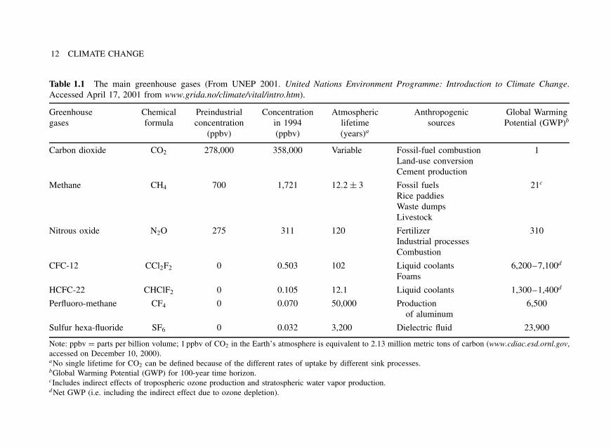
cumulative effects of these gases on theEarth’s climate, we need to examine theirtotal quantity, their natural and human sourcesto the atmosphere, their rates of loss tonatural sinks, their past and projected rates ofincrease, and their individual and cumulativeheating capacities (Table 1.1).
Water vapor traps heat in the atmosphereand makes the greatest contribution to thegreenhouse effect. Its level in the atmosphereis not directly the result of human activities.However, because warmer air can hold morewater vapor, an increase in the Earth’stemperature resulting from other greenhousegases produces a “positive feedback,” that is,more warming means more water vapor inthe atmosphere, which in turn contributes tofurther warming (Chapter 3).
Carbon dioxide is a natural componentof the atmosphere and is very biologicallyreactive. It can be reduced to organic car-bon biomass through photosynthetic uptakein plants and, through biological oxidation(respiration), converted back to gaseous CO2
and returned to the atmosphere. Major naturalsources to the atmosphere are animal respi-ration, microbial breakdown of dead organicmatter and soil carbon, and ocean to atmo-sphere exchange (flux). Sinks include photo-synthetic uptake by plants and atmosphere toocean flux. These natural cycles maintainedthe atmospheric concentration of CO2 at about280 ± 10 ppmv (parts per million by volume)for several thousand years prior to industrial-ization in the mid-nineteenth century.
During the past 150 years, and especiallyduring the last few decades, humans greatlyincreased the concentration of atmosphericCO2. Huge reservoirs of carbon, stored formillions of years as fossilized organic car-bon (coal, oil, and gas) in the Earth’s crust,have been removed and burned for fuel.When carbon fuels burn, they combine with
12 CLIMATE CHANGE
Table 1.1 The main greenhouse gases (From UNEP 2001. United Nations Environment Programme: Introduction to Climate Change.Accessed April 17, 2001 from www.grida.no/climate/vital/intro.htm).
Greenhousegases
Chemicalformula
Preindustrialconcentration
(ppbv)
Concentrationin 1994(ppbv)
Atmosphericlifetime(years)a
Anthropogenicsources
Global WarmingPotential (GWP)b
Carbon dioxide CO2 278,000 358,000 Variable Fossil-fuel combustionLand-use conversionCement production
1
Methane CH4 700 1,721 12.2 ± 3 Fossil fuelsRice paddiesWaste dumpsLivestock
21c
Nitrous oxide N2O 275 311 120 FertilizerIndustrial processesCombustion
310
CFC-12 CCl2F2 0 0.503 102 Liquid coolantsFoams
6,200–7,100d
HCFC-22 CHClF2 0 0.105 12.1 Liquid coolants 1,300–1,400d
Perfluoro-methane CF4 0 0.070 50,000 Productionof aluminum
6,500
Sulfur hexa-fluoride SF6 0 0.032 3,200 Dielectric fluid 23,900
Note: ppbv = parts per billion volume; 1 ppbv of CO2 in the Earth’s atmosphere is equivalent to 2.13 million metric tons of carbon (www.cdiac.esd.ornl.gov,accessed on December 10, 2000).aNo single lifetime for CO2 can be defined because of the different rates of uptake by different sink processes.bGlobal Warming Potential (GWP) for 100-year time horizon.cIncludes indirect effects of tropospheric ozone production and stratospheric water vapor production.dNet GWP (i.e. including the indirect effect due to ozone depletion).
EARTH AND THE GREENHOUSE EFFECT 13
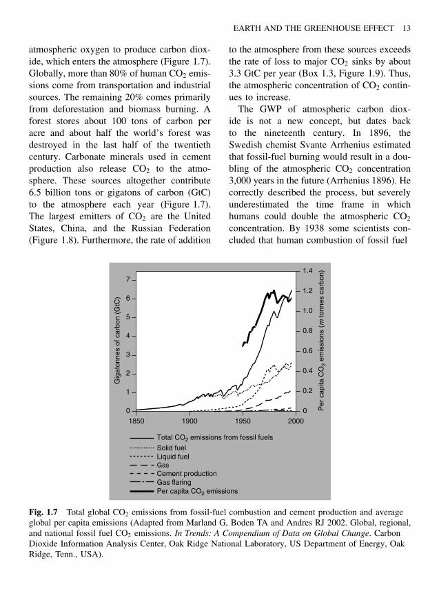
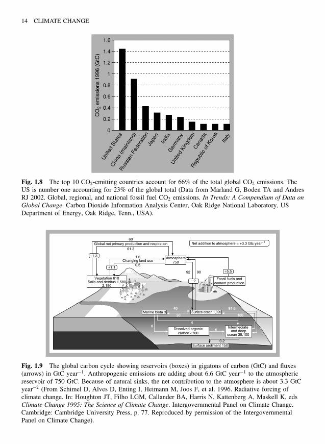
atmospheric oxygen to produce carbon diox-ide, which enters the atmosphere (Figure 1.7).Globally, more than 80% of human CO2 emis-sions come from transportation and industrialsources. The remaining 20% comes primarilyfrom deforestation and biomass burning. Aforest stores about 100 tons of carbon peracre and about half the world’s forest wasdestroyed in the last half of the twentiethcentury. Carbonate minerals used in cementproduction also release CO2 to the atmo-sphere. These sources altogether contribute6.5 billion tons or gigatons of carbon (GtC)to the atmosphere each year (Figure 1.7).The largest emitters of CO2 are the UnitedStates, China, and the Russian Federation(Figure 1.8). Furthermore, the rate of addition
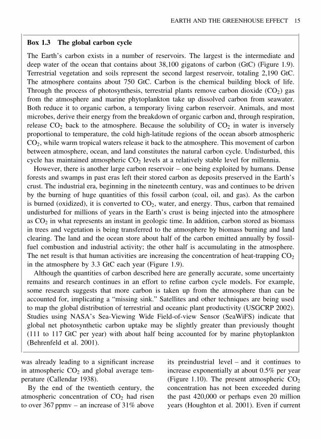
to the atmosphere from these sources exceedsthe rate of loss to major CO2 sinks by about3.3 GtC per year (Box 1.3, Figure 1.9). Thus,the atmospheric concentration of CO2 contin-ues to increase.
The GWP of atmospheric carbon diox-ide is not a new concept, but dates backto the nineteenth century. In 1896, theSwedish chemist Svante Arrhenius estimatedthat fossil-fuel burning would result in a dou-bling of the atmospheric CO2 concentration3,000 years in the future (Arrhenius 1896). Hecorrectly described the process, but severelyunderestimated the time frame in whichhumans could double the atmospheric CO2
concentration. By 1938 some scientists con-cluded that human combustion of fossil fuel
7
6
5
4
3
2
1
0
1.4
1.2
1.0
0.8
0.6
0.4
0.2
0
1850 1900 1950 2000
Gig
aton
nes
of c
arbo
n (G
tC)
Per
cap
ita C
O2
emis
sion
s (m
tonn
es c
arbo
n)
Total CO2 emissions from fossil fuels
Solid fuelLiquid fuelGasCement productionGas flaringPer capita CO2 emissions
Fig. 1.7 Total global CO2 emissions from fossil-fuel combustion and cement production and averageglobal per capita emissions (Adapted from Marland G, Boden TA and Andres RJ 2002. Global, regional,and national fossil fuel CO2 emissions. In Trends: A Compendium of Data on Global Change. CarbonDioxide Information Analysis Center, Oak Ridge National Laboratory, US Department of Energy, OakRidge, Tenn., USA).
14 CLIMATE CHANGE
1.6
1.4
1.2
1
0.8
0.6
0.4
0.2
0
CO
2 em
issi
ons
1996
(G
tC)
Uni
ted
Stat
esC
hina
(mai
nlan
d)
Rus
sian
Fed
erat
ion
Japa
nIn
dia
Ger
man
y
Can
ada
Italy
Rep
ublic
of K
orea
Uni
ted
King
dom
Fig. 1.8 The top 10 CO2-emitting countries account for 66% of the total global CO2 emissions. TheUS is number one accounting for 23% of the global total (Data from Marland G, Boden TA and AndresRJ 2002. Global, regional, and national fossil fuel CO2 emissions. In Trends: A Compendium of Data onGlobal Change. Carbon Dioxide Information Analysis Center, Oak Ridge National Laboratory, USDepartment of Energy, Oak Ridge, Tenn., USA).
Global net primary production and respiration60
61.3
1.6
92 90
0.5Changing land use
Atmosphere750
Fossil fuels andcement production
Net addition to atmosphere = +3.3 Gtc year−1
Vegetation 610Soils and detritus 1,580
2,190
−1.3
−2
+5.5+1.1
Marine biota 3
Dissolved organiccarbon <700
Surface sediment 150
Intermediate and deep
ocean 38,100
Surface ocean 1,020
0.2
6
40 91.6
100
4
50
Fig. 1.9 The global carbon cycle showing reservoirs (boxes) in gigatons of carbon (GtC) and fluxes(arrows) in GtC year−1. Anthropogenic emissions are adding about 6.6 GtC year−1 to the atmosphericreservoir of 750 GtC. Because of natural sinks, the net contribution to the atmosphere is about 3.3 GtCyear−2 (From Schimel D, Alves D, Enting I, Heimann M, Joos F, et al. 1996. Radiative forcing ofclimate change. In: Houghton JT, Filho LGM, Callander BA, Harris N, Kattenberg A, Maskell K, edsClimate Change 1995: The Science of Climate Change. Intergovernmental Panel on Climate Change.Cambridge: Cambridge University Press, p. 77. Reproduced by permission of the IntergovernmentalPanel on Climate Change).
EARTH AND THE GREENHOUSE EFFECT 15
Box 1.3 The global carbon cycle
The Earth’s carbon exists in a number of reservoirs. The largest is the intermediate anddeep water of the ocean that contains about 38,100 gigatons of carbon (GtC) (Figure 1.9).Terrestrial vegetation and soils represent the second largest reservoir, totaling 2,190 GtC.The atmosphere contains about 750 GtC. Carbon is the chemical building block of life.Through the process of photosynthesis, terrestrial plants remove carbon dioxide (CO2) gasfrom the atmosphere and marine phytoplankton take up dissolved carbon from seawater.Both reduce it to organic carbon, a temporary living carbon reservoir. Animals, and mostmicrobes, derive their energy from the breakdown of organic carbon and, through respiration,release CO2 back to the atmosphere. Because the solubility of CO2 in water is inverselyproportional to temperature, the cold high-latitude regions of the ocean absorb atmosphericCO2, while warm tropical waters release it back to the atmosphere. This movement of carbonbetween atmosphere, ocean, and land constitutes the natural carbon cycle. Undisturbed, thiscycle has maintained atmospheric CO2 levels at a relatively stable level for millennia.
However, there is another large carbon reservoir – one being exploited by humans. Denseforests and swamps in past eras left their stored carbon as deposits preserved in the Earth’scrust. The industrial era, beginning in the nineteenth century, was and continues to be drivenby the burning of huge quantities of this fossil carbon (coal, oil, and gas). As the carbonis burned (oxidized), it is converted to CO2, water, and energy. Thus, carbon that remainedundisturbed for millions of years in the Earth’s crust is being injected into the atmosphereas CO2 in what represents an instant in geologic time. In addition, carbon stored as biomassin trees and vegetation is being transferred to the atmosphere by biomass burning and landclearing. The land and the ocean store about half of the carbon emitted annually by fossil-fuel combustion and industrial activity; the other half is accumulating in the atmosphere.The net result is that human activities are increasing the concentration of heat-trapping CO2
in the atmosphere by 3.3 GtC each year (Figure 1.9).Although the quantities of carbon described here are generally accurate, some uncertainty
remains and research continues in an effort to refine carbon cycle models. For example,some research suggests that more carbon is taken up from the atmosphere than can beaccounted for, implicating a “missing sink.” Satellites and other techniques are being usedto map the global distribution of terrestrial and oceanic plant productivity (USGCRP 2002).Studies using NASA’s Sea-Viewing Wide Field-of-view Sensor (SeaWiFS) indicate thatglobal net photosynthetic carbon uptake may be slightly greater than previously thought(111 to 117 GtC per year) with about half being accounted for by marine phytoplankton(Behrenfeld et al. 2001).
was already leading to a significant increasein atmospheric CO2 and global average tem-perature (Callendar 1938).
By the end of the twentieth century, theatmospheric concentration of CO2 had risento over 367 ppmv – an increase of 31% above
its preindustrial level – and it continues toincrease exponentially at about 0.5% per year(Figure 1.10). The present atmospheric CO2
concentration has not been exceeded duringthe past 420,000 or perhaps even 20 millionyears (Houghton et al. 2001). Even if current
16 CLIMATE CHANGE
3601.5
1.0
0.5
0.0
0.5
0.4
0.3
0.2
0.1
0.0
0.15
0.10
0.05
0.0
340
320
300
280
260
1,750
1,550
1,250
1,000
750
310
290
270
2501000 1200
200
100
01600 1800
Year
2000
1400 1600 1800 2000
Carbon dioxide
Global atmospheric concentrationsof three greenhouse gases
Sulfate aerosols deposited in Greenland ice
Year
Methane
Nitrous oxide
CO
2 (p
pm)
N2O
(pp
b)A
tmos
pher
ic c
once
ntra
tion
CH
4 (p
pb)
Sul
fate
con
cent
ratio
n(m
g S
O42−
per
tonn
e of
ice)
Rad
iativ
e fo
rcin
g (W
m−2
)
Sulfur
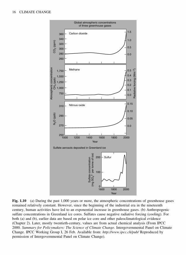
Fig. 1.10 (a) During the past 1,000 years or more, the atmospheric concentrations of greenhouse gasesremained relatively constant. However, since the beginning of the industrial era in the nineteenthcentury, human activities have led to an exponential increase in greenhouse gases. (b) Anthropogenicsulfate concentrations in Greenland ice cores. Sulfates cause negative radiative forcing (cooling). Forboth (a) and (b), earlier data are based on polar ice core and other paleoclimatological evidence(Chapter 2). Later, mostly twentieth-century, values are from actual chemical analysis (From IPCC2000. Summary for Policymakers: The Science of Climate Change. Intergovernmental Panel on ClimateChange. IPCC Working Group I, 26 Feb. Available from: http://www.ipcc.ch/pub/ Reproduced bypermission of Intergovernmental Panel on Climate Change).
EARTH AND THE GREENHOUSE EFFECT 17
CO2 emissions are reduced and maintainedat or near 1994 rates, the atmospheric con-centration will reach 500 ppmv (nearly dou-ble the preindustrial level) by the end ofthis century – far sooner than Arrhenius couldhave imagined. The major long-term reservoir(sink) for CO2 is the deep ocean. Carbon diox-ide produced today will take more than 100years to be absorbed by this reservoir. Thus,even if all emissions ceased today, atmo-spheric CO2 would remain above its prein-dustrial level for the next 100 to 300 years.
Fossil fuels are nonrenewable and theirsupply is finite. However, current supplies areabundant, relatively inexpensive, and couldlast for another 40 to 200 years (Table 1.2).If we continue to burn the carbon remainingin tropical rainforests, oil, gas, and coalreserves, we could more than quadruple theconcentration of atmospheric CO2 in the nextfew centuries.
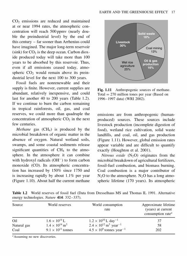
Methane gas (CH4) is produced by themicrobial breakdown of organic matter in theabsence of oxygen. Natural wetland soils,swamps, and some coastal sediments releasesignificant quantities of CH4 to the atmo-sphere. In the atmosphere it can combinewith hydroxyl radicals (OH−) to form carbonmonoxide (CO). Its atmospheric concentra-tion has increased by 150% since 1750 andis increasing rapidly by about 1.1% per year(Figure 1.10). About half the current methane
Livestock30%
Solid waste16%
Oil & gasproduction
16%
Wet riceagriculture
25%
Coal mining13%
Fig. 1.11 Anthropogenic sources of methane.Total = 270 million tones per year (Based on1996–1997 data) (WRI 2002).
emissions are from anthropogenic (human-produced) sources. These sources includelivestock production (incomplete digestion offood), wetland rice cultivation, solid wastelandfills, and coal, oil, and gas production(Figure 1.11). However, global emission ratesappear variable and are difficult to quantifyexactly (Houghton et al. 2001).
Nitrous oxide (N2O) originates from themicrobial breakdown of agricultural fertilizers,fossil-fuel combustion, and biomass burning.Coal combustion is a major contributor ofN2O to the atmosphere. N2O has a long atmo-spheric lifetime (170 years). Its atmospheric
Table 1.2 World reserves of fossil fuel (Data from Dresselhaus MS and Thomas IL 1991. Alternativeenergy technologies. Nature 414: 332–337).
Source World reserves World consumptionrate
Approximate lifetime(years) at currentconsumption ratea
Oil 1.6 × 10¹⁴ L 1.2 × 10¹⁰ L day−1 37Natural gas 1.4 × 10¹⁴ m3 2.4 × 10¹² m3 year−1 58Coal 9.1 × 10¹¹ tonnes 4.5 × 10⁹ tonnes year−1 202
aAssuming no new discoveries.

18 CLIMATE CHANGE
concentration has increased since the preindus-trial era by 16%, and it continues to increaseby about 0.25% per year. It makes a signifi-cant contribution to the overall global warming(Figure 1.10).
Chlorofluorocarbons (CFCs) and hydro-chlorofluorocarbons (HCFCs) are a rela-tively inert class of manufactured industrialcompounds containing carbon, fluorine, andchlorine atoms. They are used as coolantsin refrigerators and air conditioners, and infoam insulation, aerosol sprays, and industrialcleaning solvents. These compounds escape tothe atmosphere where they destroy the strato-spheric ozone layer that shields the Earth from
harmful ultraviolet radiation. Their role inozone depletion led to the first comprehen-sive international environmental treaty – theMontreal Protocol – to phase out the useof chlorofluorocarbons. However, CFCs andHCFCs are also greenhouse gases. The atmo-spheric concentration of CFCs has increasedrapidly since the 1960s. Although they areinvolved in the destruction of the strato-spheric ozone layer (Box 1.4), which leadsto some cooling, they still make an overallpositive contribution to greenhouse warming.The Montreal Protocol now restricts their use.However, because of their long lifetimes inthe atmosphere (60 to >100 years), they must
Box 1.4 Stratospheric ozone
The stratospheric ozone layer extends upward from about 10 to 30 miles and protects life onEarth from the Sun’s harmful ultraviolet-b radiation (UV-b, 280- to 320-nm wavelength).Ozone occurs naturally in the stratosphere and is produced and destroyed at a constantrate. But, man-made chemicals, CFCs, and halons (used in coolants, foaming agents, fireextinguishers, and solvents) are gradually destroying this “good” ozone. These ozone-depleting substances degrade slowly and can remain intact for many years as they movethrough the troposphere until they reach the stratosphere. There they are broken downby the intensity of the Sun’s ultraviolet rays and release chlorine and bromine molecules,which destroy “good” ozone. One chlorine or bromine molecule can destroy 100,000 ozonemolecules, causing ozone to disappear much faster than nature can replace it. It can takeyears for ozone-depleting chemicals to reach the stratosphere, and even though we havereduced the use of many CFCs, their impact from years past is just starting to affect theozone layer. Substances released into the air today will contribute to ozone destruction wellinto the future. Satellite observations indicate a worldwide thinning of the protective ozonelayer. The most noticeable losses occur over the North and South Poles because ozonedepletion accelerates in extremely cold weather conditions. As the stratospheric ozone layeris depleted, higher UV-b levels reach the Earth’s surface. Increased UV-b can lead to morecases of skin cancer, cataracts, and impaired immune systems. Damage to UV-b-sensitivecrops, such as soybeans, reduces yield. High-altitude ozone depletion is suspected to causedecreases in phytoplankton, a plant that grows in the ocean. Phytoplankton are an importantlink in the marine food chain and, therefore, food populations could decline. Because plants“breathe in” carbon dioxide and “breathe out” oxygen, carbon dioxide levels in the air couldalso increase. Increased UV-b radiation can be instrumental in forming more ground-level(tropospheric) or “bad” ozone pollution (Box 10.1).
EARTH AND THE GREENHOUSE EFFECT 19
be considered as significant greenhouse gases.Also, hydrofluorocarbons (HFCs), a CFC sub-stitute, and related chemicals [perfluorocarbon(PFC) and sulfur hexafluoride (SF6)] cur-rently contribute little to warming, but theirincreasing use could contribute several per-cent to warming during the twenty-first cen-tury (IPCC 2000).
Tropospheric ozone (O3) – motor vehicleemissions are the major source of this green-house gas. On clear warm days with a stableatmosphere, vehicle combustion hydrocarbonsand nitrogen oxides undergo a photochemicalreaction to produce a hazy air pollution con-dition (smog) with high concentrations ofO3 (Box 10.1). The atmospheric concentra-tion increased an estimated 20 to 50% dur-ing the twentieth century and continues toincrease at about 1% per year (Beardsley1992). In the atmosphere, chemical reactionwith hydroxyl radicals OH− results in lossof O3; however, as a result of other reac-tions, increasing atmospheric CO2 will prob-ably decrease this removal process. Globally,the degree of warming due to O3 is notwell known, but believed to be on theorder of 15% of the total warming. Tropo-spheric ozone (bad ozone) is not to be con-fused with the natural stratospheric ozonelayer (good ozone) that protects the Earthfrom excess damaging ultraviolet radiation(Box 1.4).
Aerosols are small microscopic particlesresulting from fossil-fuel and biomass com-bustion, and ore smelting. They are formedlargely from sulfur, a constituent of somefuels, particularly some high-sulfur coal andoil. Sulfate aerosols increase the acidity ofthe atmosphere and form acid rain. Theyalso reflect solar energy over a broadband,including the infrared, and thus have anegative radiative forcing or cooling effecton the atmosphere. Sulfate aerosols, unlike
the greenhouse gases discussed above, havea short lifetime in the atmosphere (daysto weeks). Globally, sulfate aerosols maybe responsible for counteracting 20 to 30%of human-induced greenhouse warming. Insome regions of the industrialized North-ern Hemisphere, the sulfate-induced coolingappears to be great enough to completely off-set the current warming effect of greenhousegases. Natural sources of aerosols such as vol-canic eruptions can also inject particles intothe atmosphere, resulting in temporary global-scale cooling events, lasting months to sev-eral years.
Other greenhouse gases in total accountfor approximately 9% the total net warming.These include carbon monoxide (CO) andnitrogen oxides (NOx) – both largely fromfossil-fuel and biomass combustion.
Black carbon (soot), from the incompletecombustion of fossil fuel, may contributesubstantially to greenhouse warming, at leaston a regional scale (Chameides and Bergin2002). It is not a gas, but the black particlesmaking up soot absorb solar radiation. Itslifetime in the atmosphere is short comparedto most greenhouse gases and its warmingpotential depends on the source and itsfate on the atmosphere. Recent studies areassessing the contribution of black carbon toglobal warming.
Warming Potentials
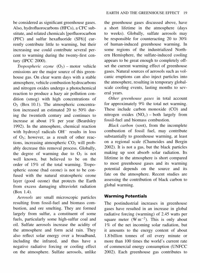
The postindustrial increases in greenhousegases have resulted in an increase in globalradiative forcing (warming) of 2.45 watts persquare meter (W m−2). This is only about1% of the net incoming solar radiation, butit amounts to the energy content of about1.8 billion tonnes of oil every minute ormore than 100 times the world’s current rateof commercial energy consumption (UNFCC2002). Each greenhouse gas contributes to
20 CLIMATE CHANGE
2.5
Rad
iativ
e fo
rcin
g w
atts
m−2
1.5
0.5
−0.5
2
1
0
CO 2CH 4
NO 2
CFCs & H
CFs
Trop
osph
eric
ozon
e
Aeros
ols
Other
gas
es
Net to
tal
Fig. 1.12 Relative contribution of anthropogenic increases in atmospheric greenhouse gasconcentrations to global radiative forcing (warming) (Data from IPCC 2000. Summary for Policymakers:The Science of Climate Change. Intergovernmental Panel on Climate Change. IPCC Working Group I,26 Feb. Available from: http://www.ipcc.ch/pub/).
this warming. Equal quantities of differentgreenhouse gases have widely different warm-ing potentials (Table 1.1). Also, the lifetimeof the gas in the atmosphere affects its resul-tant concentration and warming potential. Forexample, carbon dioxide, nitrous oxide, andCFCs have average lifetimes of 100 years ormore, whereas methane has a lifetime of 5 to10 years and carbon monoxide only 5 months.Each greenhouse gas has a characteristicper molecule greenhouse effect or warmingpotential. For example, one molecule of CFC-11 or CFC-12 traps 6 to 7 thousand timesmore heat than one molecule of CO2 andone molecule of methane traps 21 times moreheat than one molecule of CO2. However,because CO2 is much more abundant, about60% of the current human-induced green-house warming results from CO2, 15 to 20%from methane, and the remaining 20% or sofrom nitrous oxide, chlorofluorocarbons, andtropospheric ozone (Figure 1.12).
Summary
A thin layer of mixed gases surrounds theEarth. The greenhouse gases (CO2, CH4, N2O,CFCs, and O3), although less than 0.1% ofthe atmospheric volume, have a profoundinfluence on the Earth’s climate. These gases,most importantly carbon dioxide and methane,allow sunlight to penetrate, but trap outgo-ing heat. A large quantity of heat, received inthe tropics, is redistributed to higher latitudesby major atmospheric and oceanic currents.During the past 150 years, human activitieshave led to an exponential growth in green-house gas emissions. These activities includeextracting and burning fossilized carbon (coal,oil, and gas) for fuel, forest clearing and burn-ing, wetland rice cultivation, livestock rearing,solid waste landfilling, and nitrogen fertil-ization of agriculture. The result has been amajor increase in the concentrations of green-house gases, with a consequent increase in
EARTH AND THE GREENHOUSE EFFECT 21
the warming potential (heat-trapping ability)of the atmosphere.
References
Arrhenius S 1896 On the influence of carbonic acidin the air upon the temperature of the ground.Philosophical Magazine and Journal of Science,Series 5 41(251): 237–276.
Beardsley T 1992 Add ozone to the global warmingequation. Scientific American 266(3): 29.
Behrenfeld MJ, Randerson JT, McClain CR, Feld-man GC, Los SO, Tucker CJ, et al. 2001 Bio-spheric primary production during an ENSOtransition. Science 291: 2594–2597.
Callendar GS 1938 The artificial production of car-bon dioxide and its influence on temperature.Quarterly Journal of the Royal MeteorologicalSociety 64: 223–240.
CDIAC 2000 Carbon Dioxide Information AnalysisCenter, US Department of Energy, Oak RidgeNational Laboratory, http://cdiac.esd.ornl.gov.
Chameides WL and Bergin M 2002. Soot takescenter stage. Science 297: 2214, 2215.
Crutzen PJ and Ramanathan V 2000 The ascent ofatmospheric sciences. Science 290: 299–304.
Graedel TE and Crutzen PJ 1997 Atmosphere, Cli-mate, and Change. Scientific American Library,New York: W.H. Freeman, p. 3.
Hileman B 1989 Global warming. Chemical andEngineering News 19: 25–40.
IPCC 2000 Summary for Policymakers: The Scienceof Climate Change. Intergovernmental Panel onClimate Change. IPCC Working Group I, 26 Feb.Available from: http://www.ipcc.ch/pub/.
Houghton JT, Ding Y, Griggs DJ, Noguer M, vander Linden PJ, Dai X, et al. 2001 Climate change
2001: The Scientific Basis . Intergovernmental Panelon Climate Change. IPCC. Cambridge: CambridgeUniversity Press, p. 39.
Lockwood JG 1979 Causes of Climate. New York:Halsted Press, John Wiley & Sons.
Oliver JE and Hidore JJ 2002 Climatology: An Atmo-spheric Science. Upper Saddle River, NJ: PrenticeHall, p. 23.
Ramanathan V 1988 The greenhouse theory of cli-mate change: a test by an inadvertent global exper-iment. Science 240: 293–299.
Schimel D, Alves D, Enting I, Heimann M, Joos F,et al. 1996 Radiative forcing of climate change.In: Houghton JT, Filho LGM, Callander BA,Harris N, Kattenberg A, Maskell K, eds Cli-mate Change 1995: The Science of ClimateChange. Intergovernmental Panel on ClimateChange. Cambridge: Cambridge University Press,p. 77.
Thurman HV 1991 Introductory Oceanography (6th
Edition). New York: Macmillan Publishing Co.Trenberth KE, Houghton JT and Filho LGM 1995
The climate system: overview. In: Houghton JTed Climate Change 1995: The Science of Cli-mate Change. Intergovernmental Panel on ClimateChange. Cambridge: Cambridge University Press,pp. 50–64.
UNEP 2001 United Nations Environment Pro-gramme: Introduction to Climate Change. Access-ed April 17, 2001 from: www.grida.no/climate/vital/intro.htm.
UNFCC 2002 United Nations Framework Conventionon Climate Change, http://unfcc.int/resource.
USGCRP 2002 U. S. Global Change Research Pro-gram Carbon Cycle Program: An InteragencyPartnership, http://www.carboncyclescience.gov.
WRI 2002. World Resources Institute, Washington,DC, http://wri.igc.org/wri/.

This Page Intentionally Left Blank

Chapter 2
Past ClimateChange: Lessonsfrom History
“The farther backward you can look,the farther forward you are likely to see.”
Winston Churchill
“From the experience of the past we derive instructive lessons for the future.”
John Quincy Adams: US Presidential Inaugural Addresses, 1789
Introduction
Since the Earth formed more than fourbillion years ago, its climate has periodi-cally shifted from warm to cool and backagain – sometimes dramatically. Fossils, pre-served in ancient sedimentary rocks, provideevidence that populations of tropical plantsand animals once thrived in Europe and else-where, where today’s climate is cool and tem-perate. Sheets of glacial ice, a mile thick,covered much of North America only 20,000years ago. About 8,000 years ago SaharanNorth Africa, now an arid desert, was hometo numerous wetlands and lakes dotted withshoreline human settlements.
More recently, very small climate changesover the past few thousand years have greatlyimpacted human civilization. Only 1,100
years ago, Viking settlers took advantage ofa particularly mild and warm period to colo-nize a temperate area that they named “Green-land.” From there they explored, and for sometime settled in, North America. At that sametime, the great Mayan civilization of Cen-tral America collapsed. Climate change andprolonged drought is one of several compet-ing theories attempting to explain the suddenand mysterious collapse of the Maya (NOAA2002). Europe in 1816 experienced “the yearwithout a summer,” and widespread crop fail-ures resulted in food shortages and politicalunrest (Gore 1993). In New England in thatsame year, it snowed in June. The immediatecause of this global cold spell was a seriesof massive volcanic eruptions in Indonesia,which released huge quantities of dust into
Climate Change: Causes, Effects, and Solutions John T. Hardy 2003 John Wiley & Sons, Ltd ISBNs: 0-470-85018-3 (HB); 0-470-85019-1 (PB)
23
24 CLIMATE CHANGE
the atmosphere and reduced the amount ofsunlight reaching the Earth. Although coolingprobably only averaged a degree or so glob-ally, the effects were dramatic. In East Africa,written documents and oral histories coveringthe past 1,000 years suggest that local civi-lizations prospered during periods of greaterprecipitation and suffered during periods ofdrought (Verschuren et al. 2000).
Past climate changes, more than 150 yearsbefore the present (BP), occurred prior tohuman emissions of greenhouse gases. Wecan learn much about the future of ourclimate by examining past climate change.What were the extremes of past climate?How rapidly did past changes occur? Whattriggered such changes? How did past changeaffect populations of plants and animalsincluding humans? Can we use past changesto validate and test our predictive models offuture climate (Chapter 4)? In this chapterwe examine these questions and evaluate thelessons we might learn from the field ofpaleoclimatology – the study of past climates(e.g. Crowley and North 1991).
Past Climate Change – Six HistoricPeriods
Climate change occurs over time, and thedegree of change depends on the timescale wechoose to examine. Changes in the last decadeseem insignificant when compared to thoseover the past million years. Computer modelsare used to predict how human emissionsof greenhouse gases will change our climateover the next century or more (Chapter 4). Toput these predictions into context, we mustfirst examine how past climate changes havealtered the chemistry of the atmosphere andinfluenced the plants and animals of the Earth.Climate change can be described in terms ofsix major time periods (Kutzbach 1989).
First, a major cooling trend occurred morethan one billion years ago with the beginningof photosynthetic organisms. The atmospherehad a relatively high concentration of CO2,and owing to the greenhouse effect, the Earthwas correspondingly warm. However, withthe appearance of photosynthetic plants, CO2
was removed from the atmosphere and storedas organic carbon. This reduced the heat-trapping capacity of the atmosphere and ledto a major cooling trend.
Second, several hundred million years ago,the Earth experienced a period of intense tec-tonic activity involving crustal movements,continental drift, and volcanic eruptions. Mas-sive outgassing of CO2 from the Earth’s crustled to an enhanced greenhouse effect withtemperatures on average 5 ◦C warmer thannow. There was a general rise in the diversityof life forms, but at least five periods of majorspecies extinctions have occurred since.
Third, beginning about 100 million yearsago, tectonic activity subsided. Outgassingof CO2 decreased, lessening the greenhouseeffect of the atmosphere, and the climatecooled once more.
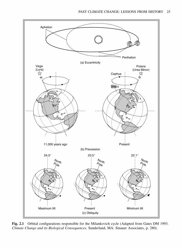
Fourth, during the past million years,shorter-term alternating cool and warm peri-ods occurred on a scale of tens of thousandsof years. These are the glacial–interglacialcycles resulting from a natural fluctuating pat-tern in the orbital configuration of the Earthwith respect to the Sun. The elliptical pathof the Earth around the Sun (eccentricity)brings it closer to or farther from the Sunevery 100,000 years (Figure 2.1a). Also, theEarth like a spinning top wobbles as it rotateson its axis, exposing more or less of eachhemisphere to the direct rays of the Sun. Itdoes this, in a process called precession, witha periodicity of 20,000 years (Figure 2.1b).Finally, the tilt of the Earth’s axis with respectto the Sun (obliquity) changes over a period
PAST CLIMATE CHANGE: LESSONS FROM HISTORY 25
Aphelion
Perihelion
(a) Eccentricity
24.5°NorthPole
Maximum tilt
23.5°NorthPole
Present
22.1°NorthPole
Minimum tilt
(c) Obliquity
(b) Precession
Vega(Lyra)
N
11,000 years ago
Cephus
Polaris(Ursa Minor)
N
Draco
Present
Fig. 2.1 Orbital configurations responsible for the Milankovich cycle (Adapted from Gates DM 1993.Climate Change and its Biological Consequences. Sunderland, MA: Sinauer Associates, p. 280).
26 CLIMATE CHANGE
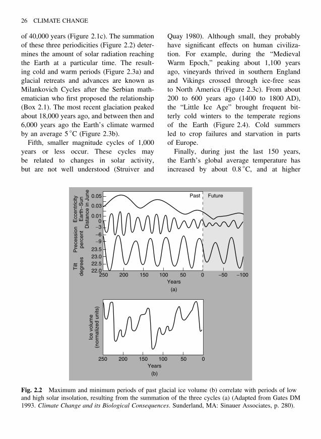
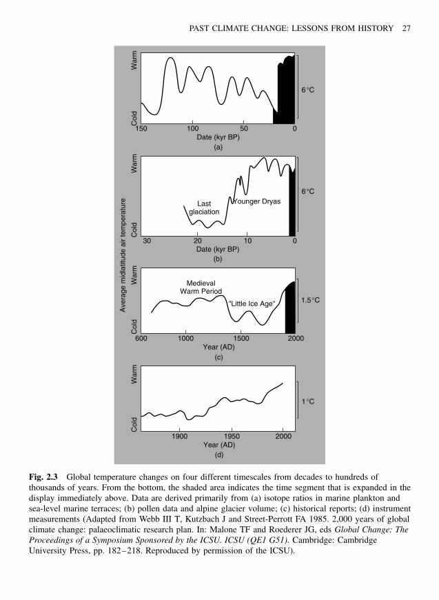
of 40,000 years (Figure 2.1c). The summationof these three periodicities (Figure 2.2) deter-mines the amount of solar radiation reachingthe Earth at a particular time. The result-ing cold and warm periods (Figure 2.3a) andglacial retreats and advances are known asMilankovich Cycles after the Serbian math-ematician who first proposed the relationship(Box 2.1). The most recent glaciation peakedabout 18,000 years ago, and between then and6,000 years ago the Earth’s climate warmedby an average 5 ◦C (Figure 2.3b).
Fifth, smaller magnitude cycles of 1,000years or less occur. These cycles maybe related to changes in solar activity,but are not well understood (Struiver and
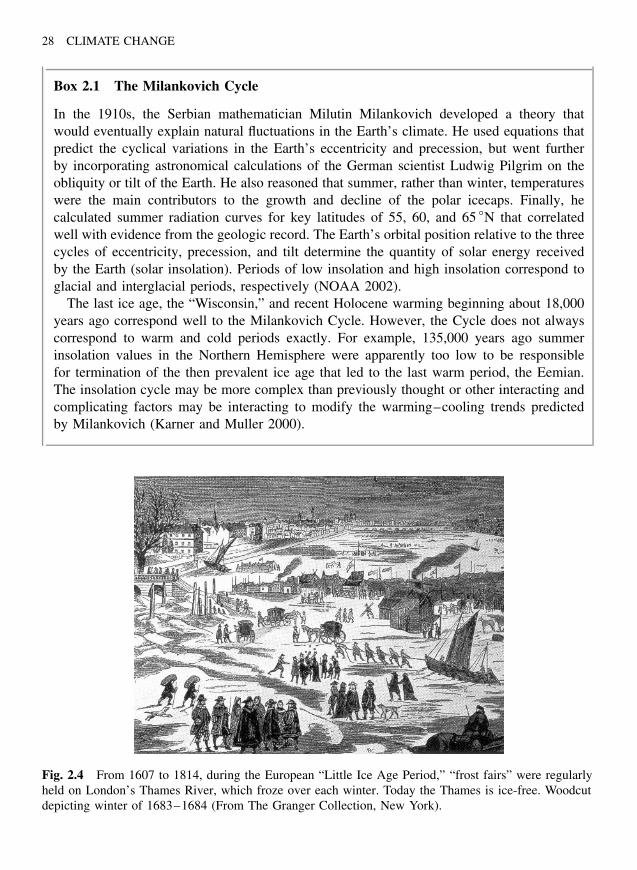
Quay 1980). Although small, they probablyhave significant effects on human civiliza-tion. For example, during the “MedievalWarm Epoch,” peaking about 1,100 yearsago, vineyards thrived in southern Englandand Vikings crossed through ice-free seasto North America (Figure 2.3c). From about200 to 600 years ago (1400 to 1800 AD),the “Little Ice Age” brought frequent bit-terly cold winters to the temperate regionsof the Earth (Figure 2.4). Cold summersled to crop failures and starvation in partsof Europe.
Finally, during just the last 150 years,the Earth’s global average temperature hasincreased by about 0.8 ◦C, and at higher
250 200 150 100 050Years
Ice
volu
me
(nor
mal
ized
uni
ts)
(b)
0.05
0.03
0.010
−3−6−9
23.523.022.522.0
250 200 150 100 050Years
(a)
−50 −100
Ecc
entr
icity
Ear
th−S
unD
ista
nce
in J
une
Pre
cess
ion
perc
ent
Tilt
degr
ees
Past Future
Fig. 2.2 Maximum and minimum periods of past glacial ice volume (b) correlate with periods of lowand high solar insolation, resulting from the summation of the three cycles (a) (Adapted from Gates DM1993. Climate Change and its Biological Consequences. Sunderland, MA: Sinauer Associates, p. 280).
PAST CLIMATE CHANGE: LESSONS FROM HISTORY 27
150 100 50Date (kyr BP)
(a)
0W
arm
Col
d
6°C
War
mC
old
1°C
1900 1950Year (AD)
(d)
2000
War
mC
old
1.5°C
600 1000 1500Year (AD)
(c)
2000
War
mC
old
6°C
30 20 10Date (kyr BP)
(b)
0
Younger DryasLastglaciation
Ave
rage
mid
latit
ude
air
tem
pera
ture
MedievalWarm Period
"Little Ice Age"
Fig. 2.3 Global temperature changes on four different timescales from decades to hundreds ofthousands of years. From the bottom, the shaded area indicates the time segment that is expanded in thedisplay immediately above. Data are derived primarily from (a) isotope ratios in marine plankton andsea-level marine terraces; (b) pollen data and alpine glacier volume; (c) historical reports; (d) instrumentmeasurements (Adapted from Webb III T, Kutzbach J and Street-Perrott FA 1985. 2,000 years of globalclimate change: palaeoclimatic research plan. In: Malone TF and Roederer JG, eds Global Change: TheProceedings of a Symposium Sponsored by the ICSU. ICSU (QE1 G51). Cambridge: CambridgeUniversity Press, pp. 182–218. Reproduced by permission of the ICSU).
28 CLIMATE CHANGE
Box 2.1 The Milankovich Cycle
In the 1910s, the Serbian mathematician Milutin Milankovich developed a theory thatwould eventually explain natural fluctuations in the Earth’s climate. He used equations thatpredict the cyclical variations in the Earth’s eccentricity and precession, but went furtherby incorporating astronomical calculations of the German scientist Ludwig Pilgrim on theobliquity or tilt of the Earth. He also reasoned that summer, rather than winter, temperatureswere the main contributors to the growth and decline of the polar icecaps. Finally, hecalculated summer radiation curves for key latitudes of 55, 60, and 65 ◦N that correlatedwell with evidence from the geologic record. The Earth’s orbital position relative to the threecycles of eccentricity, precession, and tilt determine the quantity of solar energy receivedby the Earth (solar insolation). Periods of low insolation and high insolation correspond toglacial and interglacial periods, respectively (NOAA 2002).
The last ice age, the “Wisconsin,” and recent Holocene warming beginning about 18,000years ago correspond well to the Milankovich Cycle. However, the Cycle does not alwayscorrespond to warm and cold periods exactly. For example, 135,000 years ago summerinsolation values in the Northern Hemisphere were apparently too low to be responsiblefor termination of the then prevalent ice age that led to the last warm period, the Eemian.The insolation cycle may be more complex than previously thought or other interacting andcomplicating factors may be interacting to modify the warming–cooling trends predictedby Milankovich (Karner and Muller 2000).
Fig. 2.4 From 1607 to 1814, during the European “Little Ice Age Period,” “frost fairs” were regularlyheld on London’s Thames River, which froze over each winter. Today the Thames is ice-free. Woodcutdepicting winter of 1683–1684 (From The Granger Collection, New York).
PAST CLIMATE CHANGE: LESSONS FROM HISTORY 29
latitudes has increased by several degrees Cel-sius. Although small in magnitude, this is avery rapid rate of increase, unprecedented inthe Earth’s long history.
Thus, the Earth has undergone periodicnatural fluctuations in climate of about ±1 to6 ◦C. We are currently in a warm interglacialperiod and the Earth is about as warm as ithas been for 140,000 years.
Methods of Determining PastClimates and Ecosystems
One million or even ten thousand years ago,humans were not collecting climatologicaldata. So, how do we know what the climate waslike long ago? Scientists use a number of tech-niques, each appropriate for different periodsof the past. Fossilized remains of ancient life
Box 2.2 Isotopic temperature and age determinations
Oxygen – Three isotopes of oxygen occur naturally: 16O, 17O, and 18O. Water (H2O) containsboth the light isotope (16O) and the much rarer heavy isotope (18O). These oxygen isotopescan be used to indicate past temperature and water evaporation patterns. When waterevaporates, the lighter isotope (H16
2 O) evaporates at a faster rate. Therefore, the ratio of18O to 16O in rain, snow, and ice decreases as the air temperature, and thus evaporation,increases. The reverse happens when water condenses and the heavier H18
2 O preferentiallycondenses compared to H16
2 O. Thus, the ratio of 18O to 16O in lake water is controlledmainly by the balance between evaporation and precipitation.
Carbonates – Foraminifera are tiny animals that form part of the marine planktoncommunity. When living, they deposit calcium carbonate (CaCO3) from seawater to formtheir cell walls. When they die, they settle and form ocean floor deposits. In core samplesfrom the ocean floor, the deeper ocean sediments contain the oldest deposits. The 18O/16Oratio in the CaCO3 shells of the foraminifera indicates the isotopic composition and henceseawater temperature at the time they lived. Similarly, reef-building corals deposit calciumcarbonate skeletons, and cores from old reefs can reveal the temperature of the ocean at thetime the animals lived.
Alkenones – some marine phytoplankton produce straight chain hydrocarbons calledalkenones. The colder the temperature where the phytoplankton lives, the greater the numberof double bonds in the alkenone chains of their cell membranes. When the plankton die,they settle to the ocean bottom and their alkenones are incorporated in the sediment. Thus,analysis of the ratio of different alkenones in ocean sediments indicates the past temperatureof the seawater.
Carbon – Carbon-14 is a radioactive isotope that occurs naturally in the atmospherein very low concentrations, and through photosynthesis, is incorporated in plants alongwith the much more abundant and stable 12C form of carbon. When an organism diesand is no longer accumulating carbon, the 14C slowly decays to 12C over time with ahalf-life (the time for 1/2 of the original amount to decay) of 5,730 years. Thus, theratio of 14C/12C declines over time and can be used to date the age of the animal orplant remains.

30 CLIMATE CHANGE
forms, preserved in rock formations, can indi-cate the types of species inhabiting a regionmillions of years ago. Their relationship topresent-day tropical or temperate species, or todesert or rainforest species, along with infor-mation on continental drift, can suggest thetype of climate that existed at that time.
Oxygen isotope ratios are used to determinepast temperatures and rates of precipitationand evaporation that occurred tens of thou-sands to a million years ago (Box 2.2).Oxygen bubbles trapped in ancient polar
ice deposits indicate past climate conditions.Samples of calcium carbonate, depositedby living organisms such as corals andmarine plankton, and subsequently preservedin reef structures or sediments, can revealpast ocean temperatures during the life ofthe organism (Figure 2.5). For example, esti-mates of past sea-surface temperatures fromfossil coral indicate that 10,200 years ago,waters of the tropical southwestern PacificOcean were 5 ◦C colder than today (Becket al. 1992).
Fig. 2.5 Scientists drilling a core from a large colony of the coral Porites lobata at Clipperton Atoll inthe Pacific. The core will be sectioned, age-dated, and the oxygen isotope ratios preserved in the CaCO3
skeleton at the time of live deposition, which is used to construct a record of past ocean temperatures(From NOAA 2002. National Oceanic and Atmospheric Administration Paleoclimatology Program,http://www.ngdc.noaa.gov/paleo/slides).
PAST CLIMATE CHANGE: LESSONS FROM HISTORY 31
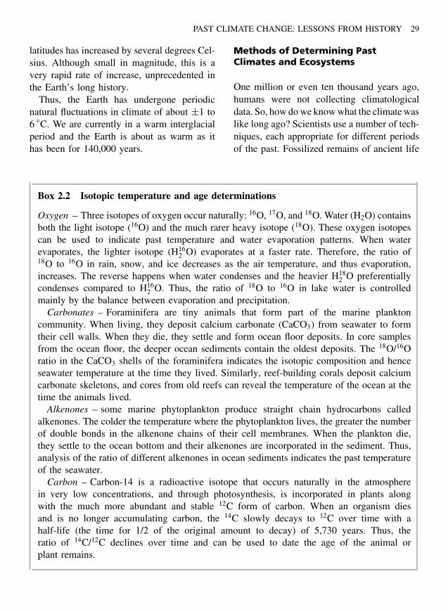
Polar ice cores have provided invaluableinsights to climate over the past 150,000years. Each year, snow deposits to formsurface ice, which is then buried the nextyear. The ice thus provides a stratigraphicrecord from the recent (shallow) to the dis-tant past (deep). In 1982, Russian scientists,using techniques similar to drilling an oilwell, removed cores of ice from the Antarc-tic ice sheet down to a depth of 2,083 m.
Sections of the “Vostok” core and from sub-sequent deep ice cores provide material forseveral types of analyses (Figure 2.6) (Ray-naud et al. 1993). Analysis of the concentra-tions of CO2 and methane (CH4) in the airbubbles trapped within the ice indicated thatof these the greenhouse gases showed simi-lar parallel fluctuations in atmospheric con-centration over different depths (past times)(Figure 2.7).
Fig. 2.6 Removing ice from a core just recovered from 90 m deep at Siple Dome, Antarctica. The drillis on the sled beside the core. In the background is the support tower for a larger drill that can recovercores to a depth of 1,000 m (From Taylor K 1999. Rapid climate change. American Scientist 87:320–327).
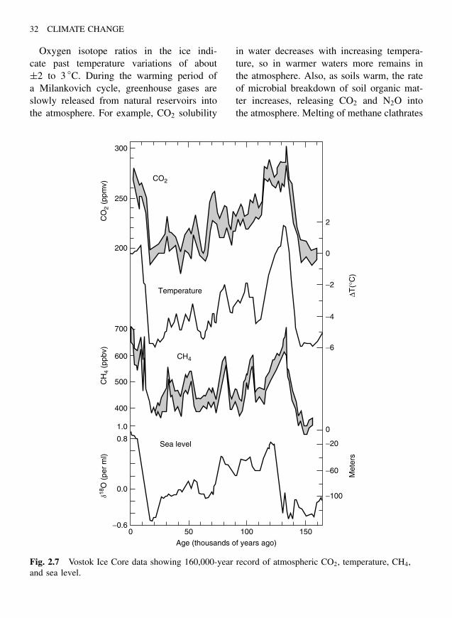
32 CLIMATE CHANGE
Oxygen isotope ratios in the ice indi-cate past temperature variations of about±2 to 3 ◦C. During the warming period ofa Milankovich cycle, greenhouse gases areslowly released from natural reservoirs intothe atmosphere. For example, CO2 solubility
in water decreases with increasing tempera-ture, so in warmer waters more remains inthe atmosphere. Also, as soils warm, the rateof microbial breakdown of soil organic mat-ter increases, releasing CO2 and N2O intothe atmosphere. Melting of methane clathrates
300
250
200
700
600
500
400
1.0
0.8
0.0
−0.60 50 100
Age (thousands of years ago)
150
CO2
CH4
Temperature
Sea level
2
0
−2
−4
−6
−20
−60
−100
0
∆T(°
C)
Met
ers
CO
2 (p
pmv)
CH
4 (p
pbv)
d18O
(pe
r m
l)
Fig. 2.7 Vostok Ice Core data showing 160,000-year record of atmospheric CO2, temperature, CH4,and sea level.
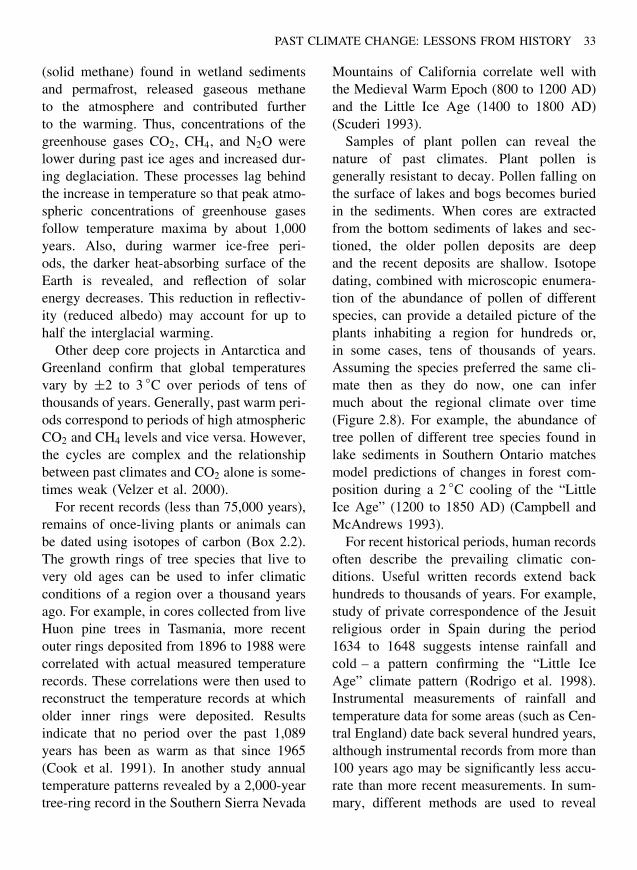
PAST CLIMATE CHANGE: LESSONS FROM HISTORY 33
(solid methane) found in wetland sedimentsand permafrost, released gaseous methaneto the atmosphere and contributed furtherto the warming. Thus, concentrations of thegreenhouse gases CO2, CH4, and N2O werelower during past ice ages and increased dur-ing deglaciation. These processes lag behindthe increase in temperature so that peak atmo-spheric concentrations of greenhouse gasesfollow temperature maxima by about 1,000years. Also, during warmer ice-free peri-ods, the darker heat-absorbing surface of theEarth is revealed, and reflection of solarenergy decreases. This reduction in reflectiv-ity (reduced albedo) may account for up tohalf the interglacial warming.
Other deep core projects in Antarctica andGreenland confirm that global temperaturesvary by ±2 to 3 ◦C over periods of tens ofthousands of years. Generally, past warm peri-ods correspond to periods of high atmosphericCO2 and CH4 levels and vice versa. However,the cycles are complex and the relationshipbetween past climates and CO2 alone is some-times weak (Velzer et al. 2000).
For recent records (less than 75,000 years),remains of once-living plants or animals canbe dated using isotopes of carbon (Box 2.2).The growth rings of tree species that live tovery old ages can be used to infer climaticconditions of a region over a thousand yearsago. For example, in cores collected from liveHuon pine trees in Tasmania, more recentouter rings deposited from 1896 to 1988 werecorrelated with actual measured temperaturerecords. These correlations were then used toreconstruct the temperature records at whicholder inner rings were deposited. Resultsindicate that no period over the past 1,089years has been as warm as that since 1965(Cook et al. 1991). In another study annualtemperature patterns revealed by a 2,000-yeartree-ring record in the Southern Sierra Nevada
Mountains of California correlate well withthe Medieval Warm Epoch (800 to 1200 AD)and the Little Ice Age (1400 to 1800 AD)(Scuderi 1993).
Samples of plant pollen can reveal thenature of past climates. Plant pollen isgenerally resistant to decay. Pollen falling onthe surface of lakes and bogs becomes buriedin the sediments. When cores are extractedfrom the bottom sediments of lakes and sec-tioned, the older pollen deposits are deepand the recent deposits are shallow. Isotopedating, combined with microscopic enumera-tion of the abundance of pollen of differentspecies, can provide a detailed picture of theplants inhabiting a region for hundreds or,in some cases, tens of thousands of years.Assuming the species preferred the same cli-mate then as they do now, one can infermuch about the regional climate over time(Figure 2.8). For example, the abundance oftree pollen of different tree species found inlake sediments in Southern Ontario matchesmodel predictions of changes in forest com-position during a 2 ◦C cooling of the “LittleIce Age” (1200 to 1850 AD) (Campbell andMcAndrews 1993).
For recent historical periods, human recordsoften describe the prevailing climatic con-ditions. Useful written records extend backhundreds to thousands of years. For example,study of private correspondence of the Jesuitreligious order in Spain during the period1634 to 1648 suggests intense rainfall andcold – a pattern confirming the “Little IceAge” climate pattern (Rodrigo et al. 1998).Instrumental measurements of rainfall andtemperature data for some areas (such as Cen-tral England) date back several hundred years,although instrumental records from more than100 years ago may be significantly less accu-rate than more recent measurements. In sum-mary, different methods are used to reveal
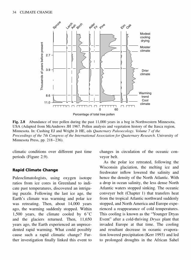
34 CLIMATE CHANGE
2.7
3.9
8.6
11.0
0 60
Percentage of total tree pollen
Spruc
e
Larc
hAsh Birc
hAlde
rFir Pine Elm Oak
Modestcoolingdrying
Moisterclimate
Drierclimate
Tho
usan
ds o
f yea
rs b
efor
e pr
esen
t
WarmingtrendCool
climate
Fig. 2.8 Abundance of tree pollen during the past 11,000 years in a bog in Northwestern Minnesota,USA (Adapted from McAndrews JH 1967. Pollen analysis and vegetation history of the Itasca region,Minnesota. In: Cushing EJ and Wright Jr HE, eds Quaternary Paleoecology. Volume 7 of theProceedings of the 7th Congress of the International Association for Quaternary Research. University ofMinnesota Press, pp. 218–236).
climatic conditions over different past timeperiods (Figure 2.9).
Rapid Climate Change
Paleoclimatologists, using oxygen isotoperatios from ice cores in Greenland to indi-cate past temperatures, discovered an intrigu-ing puzzle. Following the last ice age, theEarth’s climate was warming and polar icewas retreating. Then, about 14,000 yearsago, the warming suddenly stopped. Within1,500 years, the climate cooled by 6 ◦Cand the glaciers returned. Then, 11,650years ago, the Earth experienced an unprece-dented rapid warming. What could possiblycause such a rapid climatic change? Fur-ther investigation finally linked this event to
changes in circulation of the oceanic con-veyor belt.
As the polar ice retreated, following theWisconsin glaciation, the melting ice andfreshwater inflow lowered the salinity andhence the density of the North Atlantic. Witha drop in ocean salinity, the less dense NorthAtlantic waters stopped sinking. The oceanicconveyer belt (Chapter 1) that transfers heatfrom the tropical Atlantic northward suddenlystopped, and North America and Europe expe-rienced a reappearance of cold temperatures.This cooling is known as the “Younger DryasEvent” after a cold-thriving Dryas plant thatinvaded Europe at that time. The coolingand resultant decrease in oceanic evapora-tion lowered precipitation (Kerr 1993) and ledto prolonged droughts in the African Sahel
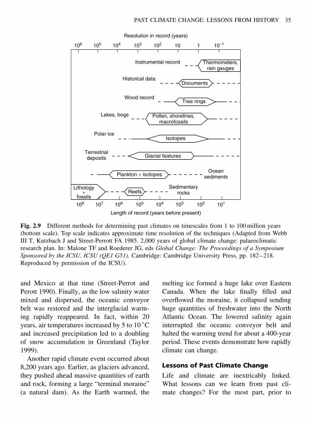
PAST CLIMATE CHANGE: LESSONS FROM HISTORY 35
106 105 104 103
Instrumental record
Historical data
Wood record
Lakes, bogs
Polar ice
102 10−110 1
108 107 106 105 104
Length of record (years before present)
Resolution in record (years)
101103 102
Terrestrialdeposits
Thermometers,rain gauges
Documents
Tree rings
Pollen, shorelines,macrofossils
Isotopes
Glacial features
Oceansediments
Sedimentaryrocks
Plankton + isotopes
ReefsLithology
+fossils
Fig. 2.9 Different methods for determining past climates on timescales from 1 to 100 million years(bottom scale). Top scale indicates approximate time resolution of the techniques (Adapted from WebbIII T, Kutzbach J and Street-Perrott FA 1985. 2,000 years of global climate change: palaeoclimaticresearch plan. In: Malone TF and Roederer JG, eds Global Change: The Proceedings of a SymposiumSponsored by the ICSU. ICSU (QE1 G51). Cambridge: Cambridge University Press, pp. 182–218.Reproduced by permission of the ICSU).
and Mexico at that time (Street-Perrot andPerott 1990). Finally, as the low salinity watermixed and dispersed, the oceanic conveyorbelt was restored and the interglacial warm-ing rapidly reappeared. In fact, within 20years, air temperatures increased by 5 to 10 ◦Cand increased precipitation led to a doublingof snow accumulation in Greenland (Taylor1999).
Another rapid climate event occurred about8,200 years ago. Earlier, as glaciers advanced,they pushed ahead massive quantities of earthand rock, forming a large “terminal moraine”(a natural dam). As the Earth warmed, the
melting ice formed a huge lake over EasternCanada. When the lake finally filled andoverflowed the moraine, it collapsed sendinghuge quantities of freshwater into the NorthAtlantic Ocean. The lowered salinity againinterrupted the oceanic conveyor belt andhalted the warming trend for about a 400-yearperiod. These events demonstrate how rapidlyclimate can change.
Lessons of Past Climate Change
Life and climate are inextricably linked.What lessons can we learn from past cli-mate changes? For the most part, prior to
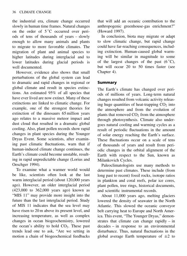
36 CLIMATE CHANGE
the industrial era, climate change occurredslowly in human time frames. Natural changeson the order of 5 ◦C occurred over peri-ods of tens of thousands of years – slowlyenough to allow many animals and plantsto migrate to more favorable climates. Themigration of plant and animal species tohigher latitudes during interglacial and tolower latitudes during glacial periods iswell documented.
However, evidence also shows that smallperturbations of the global system can leadto dramatic and rapid changes in regional orglobal climate and result in species extinc-tions. An estimated 95% of all species thathave ever lived are now extinct. Many of theseextinctions are linked to climatic change. Forexample, one of the strongest theories forextinction of the dinosaurs 65 million yearsago relates to a massive meteor impact anddust cloud that resulted in a dramatic globalcooling. Also, plant pollen records show rapidchanges in plant species during the YoungerDryas Event. Some scientists, after examin-ing past climatic fluctuations, warn that ifhuman-induced climate change continues, theEarth’s climate could become unstable, result-ing in rapid unpredictable change (Lorius andOeschger 1994).
To examine what a warmer world wouldbe like, scientists often look at the lastwarm interglacial period (about 120,000 yearsago). However, an older interglacial period(423,000 to 362,000 years ago) known as“MIS 11” may provide more insight into thefuture than the last interglacial period. Studyof MIS 11 indicates that the sea level mayhave risen to 20 m above its present level, andincreasing temperature, as well as complexchanges in ocean biogeochemistry, loweredthe ocean’s ability to hold CO2. These pasttrends lead one to ask, “Are we setting inmotion a chain of biogeochemical feedbacks
that will add an oceanic contribution to theanthropogenic greenhouse-gas enrichment?”(Howard 1997).
In conclusion, biota may migrate or adaptto slow climatic change, but rapid changecould have far-reaching consequences, includ-ing extinction. Human-caused global warm-ing will be similar in magnitude to someof the largest changes of the past (6 ◦C),but will occur 20 to 50 times faster (seeChapter 4).
Summary
The Earth’s climate has changed over peri-ods of millions of years. Long-term naturalchanges resulted from volcanic activity releas-ing huge quantities of heat-trapping CO2 intothe atmosphere and from the evolution ofplants that removed CO2 from the atmospherethrough photosynthesis. Climate also under-goes natural cooling and warming cycles as aresult of periodic fluctuations in the amountof solar energy reaching the Earth’s surface.These fluctuations occur on a scale of tensof thousands of years and result from peri-odic changes in the orbital alignment of theEarth with respect to the Sun, known asMilankovich Cycles.
Paleoclimatologists use many methods todetermine past climates. These include (fromlong past to recent) fossil rocks, isotope ratiosin plankton and coral reefs, polar ice cores,plant pollen, tree rings, historical documents,and scientific instrumental records.
About 11,000 years ago, melting glacierslowered the density of seawater in the NorthAtlantic. This slowed the oceanic conveyorbelt carrying heat to Europe and North Amer-ica. This event, “The Younger Dryas,” demon-strates that climate can change rapidly – indecades – in response to an environmentaldisturbance. Thus, natural fluctuations in theglobal average Earth temperature of ±2 to
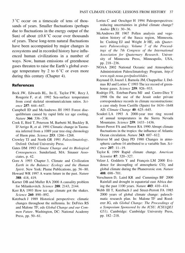
PAST CLIMATE CHANGE: LESSONS FROM HISTORY 37
3 ◦C occur on a timescale of tens of thou-sands of years. Smaller fluctuations (perhapsdue to fluctuations in the energy output of theSun) of about ±0.8 ◦C occur over thousandsof years. These long-term natural fluctuationshave been accompanied by major changes inecosystems and in recorded history have influ-enced human civilizations in a number ofways. Now, human emissions of greenhousegases threaten to raise the Earth’s global aver-age temperature by 2 to 6 ◦C or even moreduring this century (Chapter 4).
References
Beck JW, Edwards RL, Ito E, Taylor FW, Recy J,Rougerie F, et al. 1992 Sea-surface temperaturefrom coral skeletal strontium/calcium ratios. Sci-ence 257: 644–647.
Campbell ID and McAndrews JH 1993 Forest dise-quilibrium caused by rapid little ice age cooling.Nature 366: 336–338.
Cook E, Bird T, Peterson M, Barbetti M, Buckley B,D’Arrigo R, et al. 1991 Climatic change in Tasma-nia inferred from a 1089 year tree-ring chronologyof Huon pine. Science 253: 1266–1268.
Crowley TJ and North GR 1991 Paleoclimatology .Oxford: Oxford University Press.
Gates DM 1993 Climate Change and its BiologicalConsequences . Sunderland, MA: Sinauer Asso-ciates, p. 42.
Gore A 1993 Chapter 3, Climate and CivilizationEarth in the Balance: Ecology and the HumanSpirit . New York: Plume Publications, pp. 56–80.
Howard WR 1997 A warm future in the past. Nature388: 418, 419.
Karner DB and Muller RA 2000 A causality problemfor Milankovitch. Science 288: 2143, 2144.
Kerr RA 1993 How ice age climate got the shakes.Science 260: 890–892.
Kutzbach J 1989 Historical perspectives: climaticchanges throughout the millennia. In: DeFries RSand Malone TF, eds Global Change and our Com-mon Future. Washington, DC: National AcademyPress, pp. 50–61.
Lorius C and Oeschger H 1994 Paleoperspectives:reducing uncertainties in global climate change?Ambio 23(1): 30–36.
McAndrews JH 1967 Pollen analysis and vege-tation history of the Itasca region, Minnesota.In: Cushing EJ and Wright Jr HE, eds Quater-nary Paleoecology. Volume 7 of the Proceed-ings of the 7th Congress of the InternationalAssociation for Quaternary Research . Univer-sity of Minnesota Press, Minneapolis, USA,pp. 218–236.
NOAA 2002 National Oceanic and AtmosphericAdministration Paleoclimatology Program, http://www.ngdc.noaa.gov/paleo/slides .
Raynaud D, Jouzel J, Barnola JM, Chappellaz J, Del-mas RJ and Lorius C 1993 The ice record of green-house gases. Science 259: 926–933.
Rodrigo FS, Esteban-Parra MJ and Castro-Diez Y1998 On the use of the Jesuit order privatecorrespondence records in climate reconstructions:a case study from Castille (Spain) for 1634–1648AD. Climate Change 40: 625–645.
Scuderi LA 1993 A 2000-year tree ring recordof annual temperatures in the Sierra NevadaMountains. Science 259: 1433–1436.
Street-Perrot FA and Perrot RA 1990 Abrupt climatefluctuations in the tropics: the influence of AtlanticOcean circulation. Nature 343: 607–612.
Struiver M and Quay PD 1980 Changes in atmo-spheric carbon-14 attributed to a variable Sun. Sci-ence 207: 11–19.
Taylor K 1999 Rapid climate change. AmericanScientist 87: 320–327.
Velzer J, Godderis Y and Francois LM 2000 Evi-dence for decoupling of atmospheric CO2 andglobal climate during the Phanerozoic eon. Nature408: 698–701.
Verschuren D, Laird KR and Cummings BF 2000Rainfall and drought in equatorial east Africa dur-ing the past 1100 years. Nature 403: 410–414.
Webb III T, Kutzbach J and Street-Perrott FA 19852000 years of global climate change: paleocli-matic research plan. In: Malone TF and Roed-erer JG, eds Global Change: The Proceedings ofa Symposium Sponsored by the ICSU. ICSU(QE1G51). Cambridge: Cambridge University Press,pp. 182–218.

This Page Intentionally Left Blank

Chapter 3
Recent ClimateChange: The EarthResponds
“The body of statistical evidence . . . now points towards a discernible humaninfluence on global climate”
Intergovernmental Panel on Climate Change, 1995
Introduction
The Earth’s climate changed substantiallyover periods of thousands to millions of years(Chapter 2). How does recent climate changeduring the past 100 to 150 years comparewith the natural long-term fluctuations of thepast? More importantly, are recent climatechanges caused by human emissions of green-house gases?
Glaciers in the European Alps are meltingrapidly and have lost more than half theirvolume since 1850. The major water reservoirsupplying Athens, Greece, suffered nearly adecade of drought in the 1990s that leftthe lake reservoir low and threatened thewater supply of four million people. Globally,the 1998 average annual temperature wasthe greatest and that for 2001 the secondgreatest since 1860. Of the 15 warmestyears recorded during the past 150 years,10 were in the 1990s. In fact, the last
decade of the twentieth century was thewarmest in the entire global instrumentaltemperature record.
Anecdotal examples of recent unusuallywarm, dry, or wet climate extremes likethese abound (Box 3.1). They suggest thatthe climate is undergoing unnatural change.However, scientific detection of an unnatu-ral change requires demonstrating that theobserved change is significantly (in a sta-tistical sense) different from the naturalpattern of variation. Even then, establish-ing a cause–effect relationship (attribution)between human greenhouse gas emissions andglobal greenhouse warming would requireadditional evidence. Perhaps, human respon-sibility for recent climatic trends can be“proven,” as in some criminal jury trials,only by examining a large number of indi-vidual circumstantial pieces of evidence, thepreponderance of which indicate unusual,
Climate Change: Causes, Effects, and Solutions John T. Hardy 2003 John Wiley & Sons, Ltd ISBNs: 0-470-85018-3 (HB); 0-470-85019-1 (PB)
39

40 CLIMATE CHANGE
Box 3.1 Anecdotal evidence of recent unusual climate change
1995–February – Los Angeles, USA, has a record high temperature of 35 ◦C (95 ◦F),which is repeated the following year.
1996–April 4 – Seattle, USA, temperature is 5.6 ◦C (10 ◦F) greater than average andmountain snow level elevation is much greater than normal.
1998–Summer – Uncontrolled wildfires sweep through large areas of Florida, USA.1998–August – Forty-one people die of heat-related stress in Louisiana – more than
double the previous record since the state began keeping suchstatistics in 1986.
1999–July – Heat-related deaths in the US midwest climb to 250.2000–2001 – Record rainfall in the United Kingdom causes widespread flooding.2001 – The second warmest year (next to 1998) globally, since records began
(142 years).2001–2002 – November, December, and January is the warmest US winter on
record. Drought conditions prevail in 15 states from Georgia toMaine and water reservoirs in New York State are 30% belownormal.
2002–Spring – A new lake formed at the base of the rapidly melting BelvedereGlacier in the Italian Alps.
On April 15 and 16, 70 record high temperatures are set in the UnitedStates, and in New York City the temperature is 16 ◦C (29 ◦F) abovenormal. On April 25, five Western US states have droughtemergencies, mountain snow packs are 80% below normal, andmoisture levels are at record lows. April 29 – severe tornadoes hitthe Eastern United States, leaving six dead.
2002–August – The worst floods in 200 years hit central Europe with four times theaverage rainfall, leaving over 100 dead and more than $20 billionin damage.
that is, unnatural, trends. Researchers haverecently uncovered such evidence by identify-ing numerous alarming changes in the Earth’sland, air, oceans, and biota that occurred dur-ing the past 150 years. Furthermore, theserecent changes have occurred over decades,rather than over hundreds of thousands ofyears, proving human-induced climate change“beyond a reasonable doubt.”
Atmospheric TemperaturesThe twentieth century was the warmest century,and 1990 to 2000 was the warmest decade, of
the past millennium (Figure 3.1a). During thepast 150 years, the global average annual tem-perature of the Earth’s lower atmosphere, thetroposphere, has warmed about 0.6 ± 0.2 ◦C(Figure 3.1b). The recent temperature increaseis evident as a time-series anomaly (Box 3.2).Thousands of individual measurements ofnear-ground air temperatures using standardthermometers at numerous sites located aroundthe world have supported the existence of thiswarming trend (Hansen and Lebedoff 1987,Jones et al. 1999, Nicholls et al. 1996).
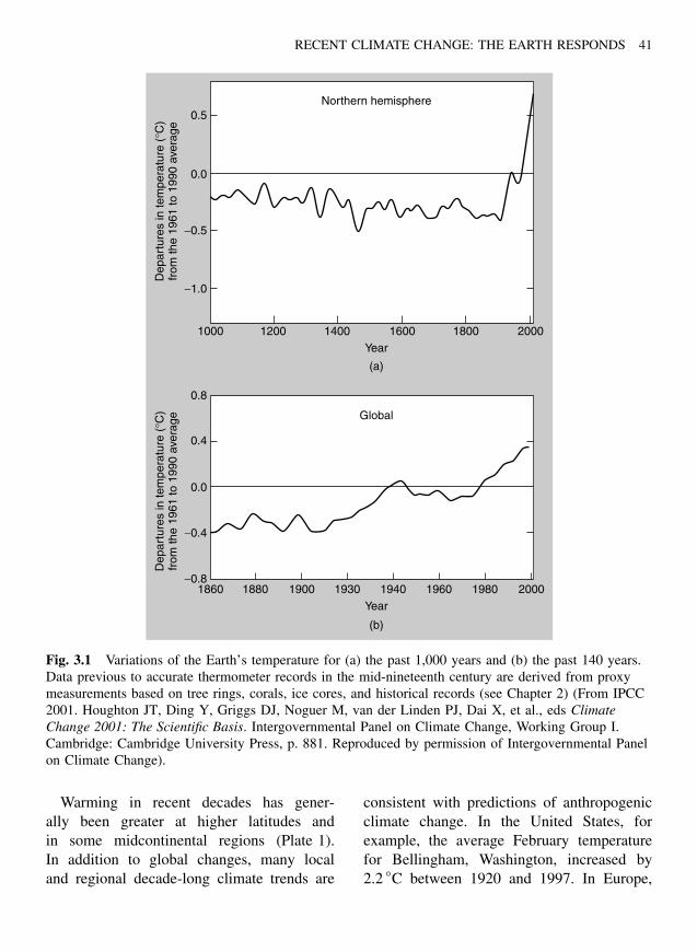
RECENT CLIMATE CHANGE: THE EARTH RESPONDS 41
0.5
0.0
0.8
0.4
0.0
−0.4
−0.8
−0.5
−1.0
1000 1200 1400 1600Year
(a)
Northern hemisphere
Dep
artu
res
in te
mpe
ratu
re (
°C)
from
the
1961
to 1
990
aver
age
Dep
artu
res
in te
mpe
ratu
re (
°C)
from
the
1961
to 1
990
aver
age
1800 2000
1860 1880 1900 1930Year
(b)
Global
1940 1960 1980 2000
Fig. 3.1 Variations of the Earth’s temperature for (a) the past 1,000 years and (b) the past 140 years.Data previous to accurate thermometer records in the mid-nineteenth century are derived from proxymeasurements based on tree rings, corals, ice cores, and historical records (see Chapter 2) (From IPCC2001. Houghton JT, Ding Y, Griggs DJ, Noguer M, van der Linden PJ, Dai X, et al., eds ClimateChange 2001: The Scientific Basis. Intergovernmental Panel on Climate Change, Working Group I.Cambridge: Cambridge University Press, p. 881. Reproduced by permission of Intergovernmental Panelon Climate Change).
Warming in recent decades has gener-ally been greater at higher latitudes andin some midcontinental regions (Plate 1).In addition to global changes, many localand regional decade-long climate trends are
consistent with predictions of anthropogenicclimate change. In the United States, forexample, the average February temperaturefor Bellingham, Washington, increased by2.2 ◦C between 1920 and 1997. In Europe,
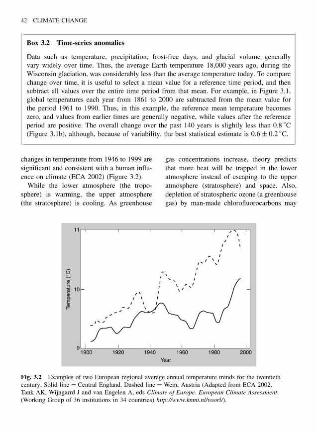
42 CLIMATE CHANGE
Box 3.2 Time-series anomalies
Data such as temperature, precipitation, frost-free days, and glacial volume generallyvary widely over time. Thus, the average Earth temperature 18,000 years ago, during theWisconsin glaciation, was considerably less than the average temperature today. To comparechange over time, it is useful to select a mean value for a reference time period, and thensubtract all values over the entire time period from that mean. For example, in Figure 3.1,global temperatures each year from 1861 to 2000 are subtracted from the mean value forthe period 1961 to 1990. Thus, in this example, the reference mean temperature becomeszero, and values from earlier times are generally negative, while values after the referenceperiod are positive. The overall change over the past 140 years is slightly less than 0.8 ◦C(Figure 3.1b), although, because of variability, the best statistical estimate is 0.6 ± 0.2 ◦C.
changes in temperature from 1946 to 1999 aresignificant and consistent with a human influ-ence on climate (ECA 2002) (Figure 3.2).
While the lower atmosphere (the tropo-sphere) is warming, the upper atmosphere(the stratosphere) is cooling. As greenhouse
gas concentrations increase, theory predictsthat more heat will be trapped in the loweratmosphere instead of escaping to the upperatmosphere (stratosphere) and space. Also,depletion of stratospheric ozone (a greenhousegas) by man-made chlorofluorocarbons may
11
10
91900 1920 1940 1960
Year
Tem
pera
ture
(°C
)
1980 2000
Fig. 3.2 Examples of two European regional average annual temperature trends for the twentiethcentury. Solid line = Central England. Dashed line = Wein, Austria (Adapted from ECA 2002.Tank AK, Wijngarrd J and van Engelen A, eds Climate of Europe. European Climate Assessment.(Working Group of 36 institutions in 34 countries) http://www.knmi.nl/voorl/).
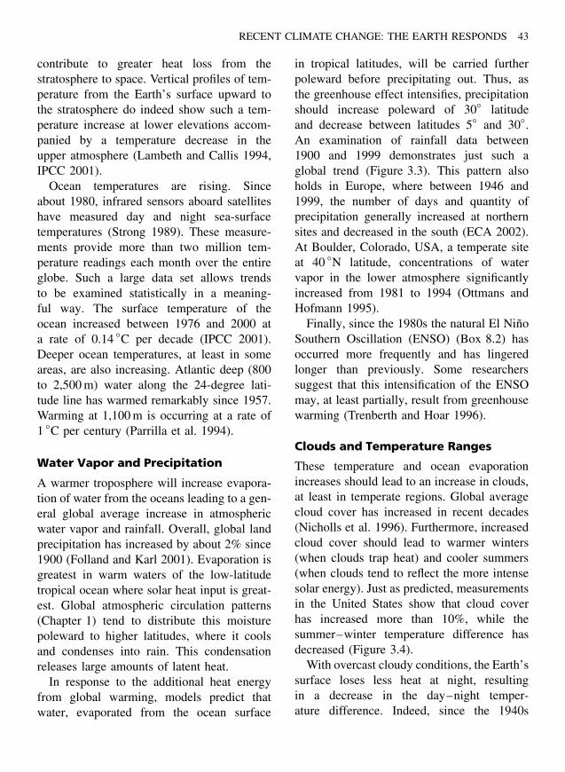
RECENT CLIMATE CHANGE: THE EARTH RESPONDS 43
contribute to greater heat loss from thestratosphere to space. Vertical profiles of tem-perature from the Earth’s surface upward tothe stratosphere do indeed show such a tem-perature increase at lower elevations accom-panied by a temperature decrease in theupper atmosphere (Lambeth and Callis 1994,IPCC 2001).
Ocean temperatures are rising. Sinceabout 1980, infrared sensors aboard satelliteshave measured day and night sea-surfacetemperatures (Strong 1989). These measure-ments provide more than two million tem-perature readings each month over the entireglobe. Such a large data set allows trendsto be examined statistically in a meaning-ful way. The surface temperature of theocean increased between 1976 and 2000 ata rate of 0.14 ◦C per decade (IPCC 2001).Deeper ocean temperatures, at least in someareas, are also increasing. Atlantic deep (800to 2,500 m) water along the 24-degree lati-tude line has warmed remarkably since 1957.Warming at 1,100 m is occurring at a rate of1 ◦C per century (Parrilla et al. 1994).
Water Vapor and Precipitation
A warmer troposphere will increase evapora-tion of water from the oceans leading to a gen-eral global average increase in atmosphericwater vapor and rainfall. Overall, global landprecipitation has increased by about 2% since1900 (Folland and Karl 2001). Evaporation isgreatest in warm waters of the low-latitudetropical ocean where solar heat input is great-est. Global atmospheric circulation patterns(Chapter 1) tend to distribute this moisturepoleward to higher latitudes, where it coolsand condenses into rain. This condensationreleases large amounts of latent heat.
In response to the additional heat energyfrom global warming, models predict thatwater, evaporated from the ocean surface
in tropical latitudes, will be carried furtherpoleward before precipitating out. Thus, asthe greenhouse effect intensifies, precipitationshould increase poleward of 30◦ latitudeand decrease between latitudes 5◦ and 30◦.An examination of rainfall data between1900 and 1999 demonstrates just such aglobal trend (Figure 3.3). This pattern alsoholds in Europe, where between 1946 and1999, the number of days and quantity ofprecipitation generally increased at northernsites and decreased in the south (ECA 2002).At Boulder, Colorado, USA, a temperate siteat 40 ◦N latitude, concentrations of watervapor in the lower atmosphere significantlyincreased from 1981 to 1994 (Ottmans andHofmann 1995).
Finally, since the 1980s the natural El NinoSouthern Oscillation (ENSO) (Box 8.2) hasoccurred more frequently and has lingeredlonger than previously. Some researcherssuggest that this intensification of the ENSOmay, at least partially, result from greenhousewarming (Trenberth and Hoar 1996).
Clouds and Temperature Ranges
These temperature and ocean evaporationincreases should lead to an increase in clouds,at least in temperate regions. Global averagecloud cover has increased in recent decades(Nicholls et al. 1996). Furthermore, increasedcloud cover should lead to warmer winters(when clouds trap heat) and cooler summers(when clouds tend to reflect the more intensesolar energy). Just as predicted, measurementsin the United States show that cloud coverhas increased more than 10%, while thesummer–winter temperature difference hasdecreased (Figure 3.4).
With overcast cloudy conditions, the Earth’ssurface loses less heat at night, resultingin a decrease in the day–night temper-ature difference. Indeed, since the 1940s
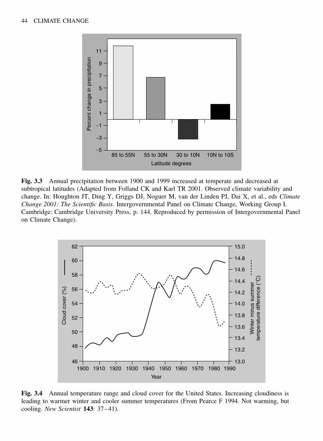
44 CLIMATE CHANGE
11
9
7
5
3
1
−1
−3
−585 to 55N 55 to 30N 30 to 10N
Latitude degrees
Per
cent
cha
nge
in p
reci
pita
tion
10N to 10S
Fig. 3.3 Annual precipitation between 1900 and 1999 increased at temperate and decreased atsubtropical latitudes (Adapted from Folland CK and Karl TR 2001. Observed climate variability andchange. In: Houghton JT, Ding Y, Griggs DJ, Noguer M, van der Linden PJ, Dai X, et al., eds ClimateChange 2001: The Scientific Basis. Intergovernmental Panel on Climate Change, Working Group I.Cambridge: Cambridge University Press, p. 144. Reproduced by permission of Intergovernmental Panelon Climate Change).
62
60
58
56
54
52
50
48
46
15.0
14.8
14.6
14.4
14.2
14.0
13.8
13.6
13.4
13.2
13.01900 1910 1920 1930 1940 1950
Year
Clo
ud c
over
(%
)
Win
ter
min
us s
umm
erte
mpe
ratu
re d
iffer
ence
(°C
)
1960 1970 1980 1990
Fig. 3.4 Annual temperature range and cloud cover for the United States. Increasing cloudiness isleading to warmer winter and cooler summer temperatures (From Pearce F 1994. Not warming, butcooling. New Scientist 143: 37–41).
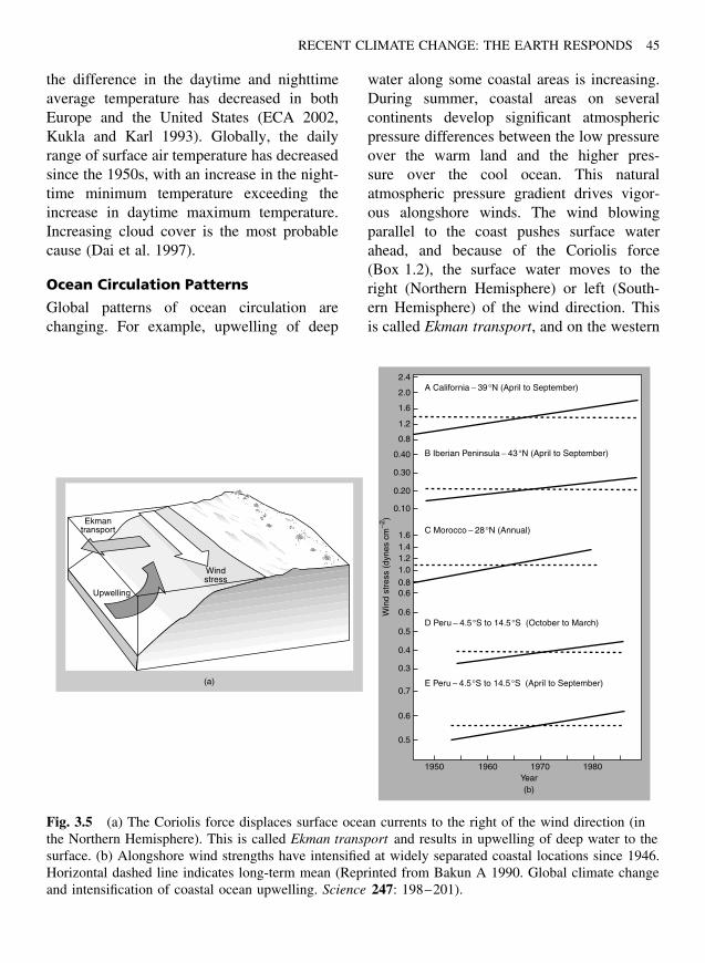
RECENT CLIMATE CHANGE: THE EARTH RESPONDS 45
the difference in the daytime and nighttimeaverage temperature has decreased in bothEurope and the United States (ECA 2002,Kukla and Karl 1993). Globally, the dailyrange of surface air temperature has decreasedsince the 1950s, with an increase in the night-time minimum temperature exceeding theincrease in daytime maximum temperature.Increasing cloud cover is the most probablecause (Dai et al. 1997).
Ocean Circulation Patterns
Global patterns of ocean circulation arechanging. For example, upwelling of deep
water along some coastal areas is increasing.During summer, coastal areas on severalcontinents develop significant atmosphericpressure differences between the low pressureover the warm land and the higher pres-sure over the cool ocean. This naturalatmospheric pressure gradient drives vigor-ous alongshore winds. The wind blowingparallel to the coast pushes surface waterahead, and because of the Coriolis force(Box 1.2), the surface water moves to theright (Northern Hemisphere) or left (South-ern Hemisphere) of the wind direction. Thisis called Ekman transport, and on the western
2.4A California − 39°N (April to September)
B Iberian Peninsula − 43°N (April to September)
C Morocco − 28°N (Annual)
D Peru − 4.5°S to 14.5°S (October to March)
E Peru − 4.5°S to 14.5°S (April to September)
2.0
1.6
1.2
0.8
0.40
0.30
0.20
0.10
1.61.41.21.0
0.80.6
0.6
0.5
0.4
0.3
0.7
0.6
0.5
1950 1960 1970Year(b)
Win
d st
ress
(dy
nes
cm−2
)
1980
Ekmantransport
Upwelling
Windstress
(a)
Fig. 3.5 (a) The Coriolis force displaces surface ocean currents to the right of the wind direction (inthe Northern Hemisphere). This is called Ekman transport and results in upwelling of deep water to thesurface. (b) Alongshore wind strengths have intensified at widely separated coastal locations since 1946.Horizontal dashed line indicates long-term mean (Reprinted from Bakun A 1990. Global climate changeand intensification of coastal ocean upwelling. Science 247: 198–201).
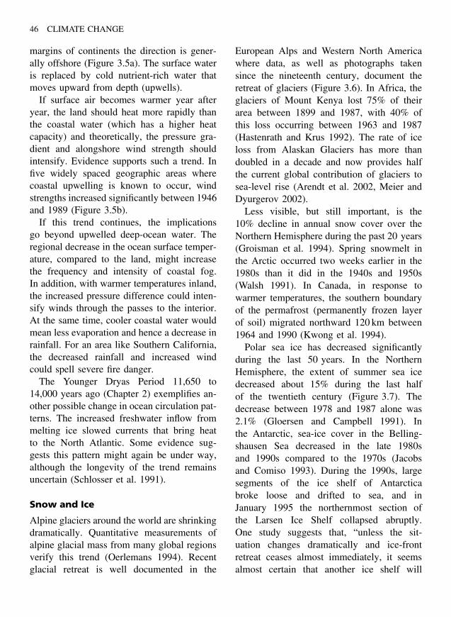
46 CLIMATE CHANGE
margins of continents the direction is gener-ally offshore (Figure 3.5a). The surface wateris replaced by cold nutrient-rich water thatmoves upward from depth (upwells).
If surface air becomes warmer year afteryear, the land should heat more rapidly thanthe coastal water (which has a higher heatcapacity) and theoretically, the pressure gra-dient and alongshore wind strength shouldintensify. Evidence supports such a trend. Infive widely spaced geographic areas wherecoastal upwelling is known to occur, windstrengths increased significantly between 1946and 1989 (Figure 3.5b).
If this trend continues, the implicationsgo beyond upwelled deep-ocean water. Theregional decrease in the ocean surface temper-ature, compared to the land, might increasethe frequency and intensity of coastal fog.In addition, with warmer temperatures inland,the increased pressure difference could inten-sify winds through the passes to the interior.At the same time, cooler coastal water wouldmean less evaporation and hence a decrease inrainfall. For an area like Southern California,the decreased rainfall and increased windcould spell severe fire danger.
The Younger Dryas Period 11,650 to14,000 years ago (Chapter 2) exemplifies an-other possible change in ocean circulation pat-terns. The increased freshwater inflow frommelting ice slowed currents that bring heatto the North Atlantic. Some evidence sug-gests this pattern might again be under way,although the longevity of the trend remainsuncertain (Schlosser et al. 1991).
Snow and Ice
Alpine glaciers around the world are shrinkingdramatically. Quantitative measurements ofalpine glacial mass from many global regionsverify this trend (Oerlemans 1994). Recentglacial retreat is well documented in the
European Alps and Western North Americawhere data, as well as photographs takensince the nineteenth century, document theretreat of glaciers (Figure 3.6). In Africa, theglaciers of Mount Kenya lost 75% of theirarea between 1899 and 1987, with 40% ofthis loss occurring between 1963 and 1987(Hastenrath and Krus 1992). The rate of iceloss from Alaskan Glaciers has more thandoubled in a decade and now provides halfthe current global contribution of glaciers tosea-level rise (Arendt et al. 2002, Meier andDyurgerov 2002).
Less visible, but still important, is the10% decline in annual snow cover over theNorthern Hemisphere during the past 20 years(Groisman et al. 1994). Spring snowmelt inthe Arctic occurred two weeks earlier in the1980s than it did in the 1940s and 1950s(Walsh 1991). In Canada, in response towarmer temperatures, the southern boundaryof the permafrost (permanently frozen layerof soil) migrated northward 120 km between1964 and 1990 (Kwong et al. 1994).
Polar sea ice has decreased significantlyduring the last 50 years. In the NorthernHemisphere, the extent of summer sea icedecreased about 15% during the last halfof the twentieth century (Figure 3.7). Thedecrease between 1978 and 1987 alone was2.1% (Gloersen and Campbell 1991). Inthe Antarctic, sea-ice cover in the Belling-shausen Sea decreased in the late 1980sand 1990s compared to the 1970s (Jacobsand Comiso 1993). During the 1990s, largesegments of the ice shelf of Antarcticabroke loose and drifted to sea, and inJanuary 1995 the northernmost section ofthe Larsen Ice Shelf collapsed abruptly.One study suggests that, “unless the sit-uation changes dramatically and ice-frontretreat ceases almost immediately, it seemsalmost certain that another ice shelf will
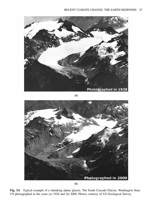
RECENT CLIMATE CHANGE: THE EARTH RESPONDS 47
(a)
(b)
Fig. 3.6 Typical example of a shrinking alpine glacier. The South Cascade Glacier, Washington StateUS photographed in the years (a) 1928 and (b) 2000. Photos courtesy of US Geological Survey.
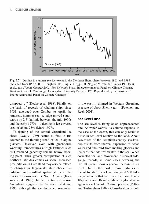
48 CLIMATE CHANGE
12
11
10
9
8
71900 1910 1920 1930 1940 1950
Year
Summer (JAS)
Sea
-ice
exte
nt (
106
km2 )
1960 1970 1980 1990 2000
Fig. 3.7 Decline in summer sea-ice extent in the Northern Hemisphere between 1901 and 1999(Adapted from IPCC 2001. Houghton JT, Ding Y, Griggs DJ, Noguer M, van der Linden PJ, Dai X,et al., eds Climate Change 2001: The Scientific Basis. Intergovernmental Panel on Climate Change,Working Group I. Cambridge: Cambridge University Press, p. 125. Reproduced by permission ofIntergovernmental Panel on Climate Change).
disappear. . .” (Doake et al. 1998). Finally, onthe basis of records of whaling ships since1931, averaged over October to April, theAntarctic summer sea-ice edge moved south-wards by 2.8◦ latitude between the mid-1950sand the early 1970s – a decline in ice-coveredarea of about 25% (Mare 1997).
Thickening of the central Greenland icesheet (Zwally 1989) seems at first to runcounter to the thinning trend of ice in alpineglaciers. However, even with greenhousewarming, temperatures at high latitudes suchas Greenland generally remain below freez-ing point. Thus, greater precipitation at suchnorthern latitudes comes as snow. Increasedprecipitation in Greenland may also be relatedto changes in large-scale atmospheric cir-culation and resultant spatial shifts in thetracks of storms over the North Atlantic (Kap-sner et al. 1995). In fact, a transect acrossGreenland suggests that between 1954 and1995, although the ice thickened somewhat
in the east, it thinned in Western Greenlandat a rate of about 31 cm year−1 (Paterson andReeh 2001).
Sea-Level Rise
The sea level is rising at an unprecedentedrate. As water warms, its volume expands. Inthe case of the ocean, this can only result ina rise in sea level relative to the land. Abouttwo-thirds of the twentieth-century sea-levelrise results from thermal expansion of oceanwater and one-third from melting glaciers andice caps that add freshwater to the sea. Whencorrected for land movement, historical tide-gauge records, in some cases covering thelast 100 years, show a general increase in sealevel. One of the most extensive studies ofrecent trends in sea level analyzed 500 tide-gauge records that had data for more than a10-year period. Results indicate a global aver-age sea-level rise of ±2.4 mm per year (Peltierand Tushingham 1989). Consideration of both
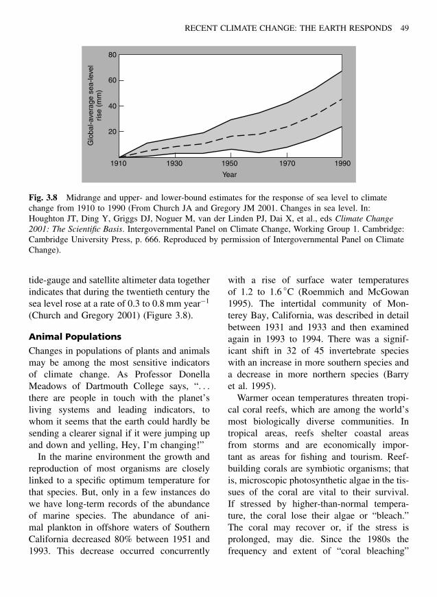
RECENT CLIMATE CHANGE: THE EARTH RESPONDS 49
80
60
40
20
1910 1930 1950
Year
Glo
bal-a
vera
ge s
ea-le
vel
rise
(mm
)
1970 1990
Fig. 3.8 Midrange and upper- and lower-bound estimates for the response of sea level to climatechange from 1910 to 1990 (From Church JA and Gregory JM 2001. Changes in sea level. In:Houghton JT, Ding Y, Griggs DJ, Noguer M, van der Linden PJ, Dai X, et al., eds Climate Change2001: The Scientific Basis. Intergovernmental Panel on Climate Change, Working Group 1. Cambridge:Cambridge University Press, p. 666. Reproduced by permission of Intergovernmental Panel on ClimateChange).
tide-gauge and satellite altimeter data togetherindicates that during the twentieth century thesea level rose at a rate of 0.3 to 0.8 mm year−1
(Church and Gregory 2001) (Figure 3.8).
Animal Populations
Changes in populations of plants and animalsmay be among the most sensitive indicatorsof climate change. As Professor DonellaMeadows of Dartmouth College says, “. . .there are people in touch with the planet’sliving systems and leading indicators, towhom it seems that the earth could hardly besending a clearer signal if it were jumping upand down and yelling, Hey, I’m changing!”
In the marine environment the growth andreproduction of most organisms are closelylinked to a specific optimum temperature forthat species. But, only in a few instances dowe have long-term records of the abundanceof marine species. The abundance of ani-mal plankton in offshore waters of SouthernCalifornia decreased 80% between 1951 and1993. This decrease occurred concurrently
with a rise of surface water temperaturesof 1.2 to 1.6 ◦C (Roemmich and McGowan1995). The intertidal community of Mon-terey Bay, California, was described in detailbetween 1931 and 1933 and then examinedagain in 1993 to 1994. There was a signif-icant shift in 32 of 45 invertebrate specieswith an increase in more southern species anda decrease in more northern species (Barryet al. 1995).
Warmer ocean temperatures threaten tropi-cal coral reefs, which are among the world’smost biologically diverse communities. Intropical areas, reefs shelter coastal areasfrom storms and are economically impor-tant as areas for fishing and tourism. Reef-building corals are symbiotic organisms; thatis, microscopic photosynthetic algae in the tis-sues of the coral are vital to their survival.If stressed by higher-than-normal tempera-ture, the coral lose their algae or “bleach.”The coral may recover or, if the stress isprolonged, may die. Since the 1980s thefrequency and extent of “coral bleaching”
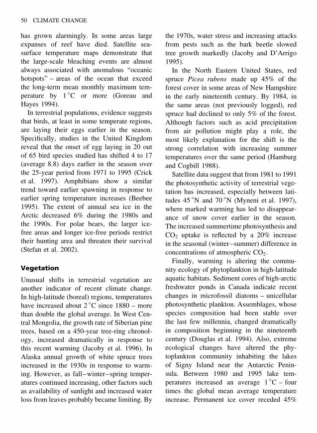
50 CLIMATE CHANGE
has grown alarmingly. In some areas largeexpanses of reef have died. Satellite sea-surface temperature maps demonstrate thatthe large-scale bleaching events are almostalways associated with anomalous “oceanichotspots” – areas of the ocean that exceedthe long-term mean monthly maximum tem-perature by 1 ◦C or more (Goreau andHayes 1994).
In terrestrial populations, evidence suggeststhat birds, at least in some temperate regions,are laying their eggs earlier in the season.Specifically, studies in the United Kingdomreveal that the onset of egg laying in 20 outof 65 bird species studied has shifted 4 to 17(average 8.8) days earlier in the season overthe 25-year period from 1971 to 1995 (Cricket al. 1997). Amphibians show a similartrend toward earlier spawning in response toearlier spring temperature increases (Beebee1995). The extent of annual sea ice in theArctic decreased 6% during the 1980s andthe 1990s. For polar bears, the larger ice-free areas and longer ice-free periods restricttheir hunting area and threaten their survival(Stefan et al. 2002).
Vegetation
Unusual shifts in terrestrial vegetation areanother indicator of recent climate change.In high-latitude (boreal) regions, temperatureshave increased about 2 ◦C since 1880 – morethan double the global average. In West Cen-tral Mongolia, the growth rate of Siberian pinetrees, based on a 450-year tree-ring chronol-ogy, increased dramatically in response tothis recent warming (Jacoby et al. 1996). InAlaska annual growth of white spruce treesincreased in the 1930s in response to warm-ing. However, as fall–winter–spring temper-atures continued increasing, other factors suchas availability of sunlight and increased waterloss from leaves probably became limiting. By
the 1970s, water stress and increasing attacksfrom pests such as the bark beetle slowedtree growth markedly (Jacoby and D’Arrigo1995).
In the North Eastern United States, redspruce Picea rubens made up 45% of theforest cover in some areas of New Hampshirein the early nineteenth century. By 1984, inthe same areas (not previously logged), redspruce had declined to only 5% of the forest.Although factors such as acid precipitationfrom air pollution might play a role, themost likely explanation for the shift is thestrong correlation with increasing summertemperatures over the same period (Hamburgand Cogbill 1988).
Satellite data suggest that from 1981 to 1991the photosynthetic activity of terrestrial vege-tation has increased, especially between lati-tudes 45 ◦N and 70 ◦N (Myneni et al. 1997),where marked warming has led to disappear-ance of snow cover earlier in the season.The increased summertime photosynthesis andCO2 uptake is reflected by a 20% increasein the seasonal (winter–summer) difference inconcentrations of atmospheric CO2.
Finally, warming is altering the commu-nity ecology of phytoplankton in high-latitudeaquatic habitats. Sediment cores of high-arcticfreshwater ponds in Canada indicate recentchanges in microfossil diatoms – unicellularphotosynthetic plankton. Assemblages, whosespecies composition had been stable overthe last few millennia, changed dramaticallyin composition beginning in the nineteenthcentury (Douglas et al. 1994). Also, extremeecological changes have altered the phy-toplankton community inhabiting the lakesof Signy Island near the Antarctic Penin-sula. Between 1980 and 1995 lake tem-peratures increased an average 1 ◦C – fourtimes the global mean average temperatureincrease. Permanent ice cover receded 45%
RECENT CLIMATE CHANGE: THE EARTH RESPONDS 51
since 1951 and the ice-free period increasedby 63 days between 1980 and 1993 (Quayleet al. 2002).
Attribution
The recent changes described above are con-sistent with a global-warming trend, but canthe warming trend be attributed to humanemissions of greenhouse gases? Human-induced changes are superimposed on naturalchanges. How can we sort out the human-induced variation (the signal) from the naturalbackground variation (the noise)? Actual attri-bution is most likely to come from an exam-ination of simultaneous patterns of changeover both space and time.
One approach is to ask if an observedchange, for example, an increase in globaltemperature, over some recent period, is sta-tistically different from any long-term natural(preindustrial) variation. Global mean tem-perature shows considerable variability on alltimescales and may show natural trends of upto 0.3 ◦C over intervals of up to 100 years.Although this natural variability is quite large,it is insufficient to explain the observed globalwarming during the twentieth century (Wigleyand Raper 1990). Several noted scientists,after examining such data, conclude that thereis an 80 to 95% probability that the globalaverage temperature increase over the past100 years is outside the range of natural vari-ation. The increase, instead, is due to humanemissions of greenhouse gases (Tol 1994,Schneider 1994).
A second approach to establishing a linkbetween global warming and human emis-sions of greenhouse gases is used by CynthiaKuo and others at the Bell Laboratories inNew Jersey. Using time-series statistics theyshow a strong positive correlation between theincreasing atmospheric concentration of car-bon dioxide and the increasing temperature
over the 30-year period that they examinedfrom 1958 to 1988. The probability that thelevel of coherence between the two variables(CO2 concentration and temperature) is due tochance alone is about 2 out of 1 million (Kuoet al. 1990).
A third approach to determining a humanlink to climate change is to compare model(expected owing to greenhouse gas increases)and observed patterns of change for a sin-gle variable (e.g. temperature) in four dimen-sions – over latitude, longitude, altitude, andtime. For example, the observed latitude ver-sus altitude changes in temperature over timefor the last few decades agree well withpatterns predicted by global climate models.Also, models predict less warming in areasof high sulfate aerosols. Observed spatial andtemporal patterns of high aerosol distributionare consistent with model predictions of areasof reduced warming (see Chapter 1).
Climate change involves much more thantemperature change. For example, in addi-tion to overall changes in temperature orprecipitation, at least five measures of cli-matic change are thought to be sensitiveto increased atmospheric concentrations ofgreenhouse gases. Multivariate statistics areused to correlate simultaneous changes inmultiple variables. Such changes includeunequal increases in maximum and minimumtemperature, increases in cold season precip-itation, severe summertime drought, and theproportion of total precipitation that is derivedfrom extreme daily precipitation events, anddecreases in day-to-day temperature varia-tions. For example, the Greenhouse ClimateResponse Index, an analysis of such changesin the United States over time since about1910, indicates that the probability that theincrease in the index since 1910 is due purelyto natural causes is only 1 to 9% (Karlet al. 1996).
52 CLIMATE CHANGE
Summary
A great deal of circumstantial events duringthe past decade or two suggests thatthe Earth’s climate is changing. Moreimportantly, scientific research on climatetrends and the Earth’s responses during thepast 150 years indicate that change is nowoccurring much more rapidly than during pasthistorical periods. There can be little doubtthat during the twentieth century, humansaltered the Earth’s climate by emittinghuge quantities of greenhouse gases. Recentchanges include
• an historically rapid tropospheric warmingof almost 1 ◦C in global average surfacetemperature and increased average sea-surface temperature;
• a stratospheric cooling, resulting fromincreased retention of heat trapped in thetroposphere due to higher greenhouse gasconcentrations;
• increased atmospheric water vapor at tem-perate latitudes, general increases in pre-cipitation poleward of 30◦ latitude, anddecreases in precipitation at lower latitudes;
• increased cloudiness and decreased day–night temperature differences at temperatelocations;
• increased coastal winds, ocean surfacecurrents, and upwelling of cold deep-ocean water along the western marginsof continents;
• decreases in snow and ice cover, shrinkingalpine glaciers, and increases in the frost-free season in temperate regions;
• an average global sea-level rise of about2.4 cm per decade;
• changes in animal populations includinggeographic shifts (poleward) of coastal
marine species populations, and earlierspring breeding of birds and amphibians;
• a dramatic increase in “bleaching” andmass mortality of coral reefs;
• changes in terrestrial and aquatic vegeta-tion, including changing growth patternsin trees and altered species composition inaquatic phytoplankton.
Statistical analyses indicate that many ofthese changes are outside the range of nat-ural variation and are consistent with modelpredictions of human-induced greenhousewarming. Predicting the magnitude of futurehuman-induced climate change remains diffi-cult and will probably come slowly as com-puter models improve (Chapter 4).
References
Arendt AA, Echelmeyer KA, Harrison WD, Lin-gle CS and Valentine VB 2002 Rapid wastage ofAlaska glaciers and their contribution to rising sealevel. Science 297: 382–386.
Bakun A 1990 Global climate change and intensi-fication of coastal ocean upwelling. Science 247:198–201.
Barry JP, Baxter CH, Sagarin RD and Gilman SE1995 Climate-related, long-term faunal changes ina California rock intertidal community. Science267: 672–674.
Beebee TJC 1995 Amphibian breeding and climate.Nature 374: 219–220.
Church JA and Gregory JM 2001 Changes in sealevel. In: Houghton JT, Ding Y, Griggs DJ,Noguer M, van der Linden PJ, Dai X, et al., eds.Climate Change 2001: The Scientific Basis . Inter-governmental Panel on Climate Change, WorkingGroup 1. Cambridge: Cambridge University Press,p. 666.
Crick HQP, Dudley C, Glue DE and Thompson DL1997 UK birds are laying eggs earlier. Nature388: 526.
Dai A, Del Genio AD and Fung IY 1997 Clouds,precipitation and temperature range. Nature 386:665, 666.
RECENT CLIMATE CHANGE: THE EARTH RESPONDS 53
de la Mare WK 1997 Abrupt mid-twentieth-centurydecline in Antarctic sea-ice extent from whalingrecords. Nature 389: 57–59.
Doake CS, Corr HFJ, Rott H, Skvarca P and YoungNW 1998 Breakup and conditions for stability ofthe northern Larsen Ice Shelf, Antarctica. Nature391: 778–780.
Douglas MSV, Smol JP and Blake Jr W 1994Marked post-18th century environmental change inhigh-arctic ecosystems. Science 266: 416–419.
ECA 2002 Tank AK, Wijngarrd J and van Enge-len A, eds Climate of Europe. European ClimateAssessment . (Working Group of 36 institutions in34 countries) http://www.knmi.nl/voorl/ .
Folland CK and Karl TR 2001 Observed climatevariability and change. In: Houghton JT, Ding Y,Griggs DJ, Noguer M, van der Linden PJ, Dai X,et al., eds Climate Change 2001: The Scien-tific Basis . Intergovernmental Panel on ClimateChange. Working Group I. Cambridge: CambridgeUniversity Press, pp. 99–181.
Gloersen P and Campbell WJ 1991 Recent variationsin Arctic and Antarctic sea-ice covers. Nature 352:33–36.
Goreau TJ and Hayes RL 1994 Coral bleaching andocean “Hot Spots”. Ambio 23(3): 176–180.
Groisman PY, Karl TR and Knight RW 1994Observed impact of snow cover on the heat balanceand the rise of continental spring temperatures.Science 263: 198–200.
Hamburg SP and Cogbill CV 1988 Historical declineof red spruce populations and climatic warming.Nature 331: 428–430.
Hansen J and Lebedoff S 1987 Global trends ofmeasured surface air temperature. Journal ofGeophysical Research 92(D11): 13,345–13,372.
Hastenrath S and Krus P 1992 The dramatic retreatof Mount Kenya’s glaciers between 1963 and1987: greenhouse forcing. Annals of Glaciology16: 127–133.
IPCC 2001 Houghton JT, Ding Y, Griggs DJ, NoguerM, van der Linden PJ, Dai X, et al., eds Cli-mate Change 2001: The Scientific Basis . Inter-governmental Panel on Climate Change. WorkingGroup I. Cambridge: Cambridge University Press.
Jacobs SS and Comiso JC 1993 A recent sea-iceretreat west of the Antarctic peninsula. Geophysi-cal Research Letters 20(12): 1171–1174.
Jacoby GC, D’Arrigo RD and Davaajamts T 1996Mongolian tree rings and 20th century warming.Science 273: 771–773.
Jacoby GC and D’Arrigo RD 1995 Tree-ring widthand density evidence of climatic and potentialforest change in Alaska. Global BiogeochemicalCycles 9(2): 227–234.
Jones PD, New M, Parker DE, Martin S and RigorIG 1999 Surface air temperature and its changesover the past 150 years. Reviews of Geophysics 37:173–199.
Kapsner WR, Aley RB, Schuman CA, Anandakrish-nan S and Grootes PM 1995 Dominant influenceof atmospheric circulation on snow accumulationin Greenland over the past 18,000 years. Nature373: 52–54.
Karl TR, Knight RW, Easterling DR and Quayle RG1996 Indices of climate change for the UnitedStates. Bulletin of the American MeteorologicalSociety 77(2): 279–292.
Kukla G and Karl TR 1993 Nighttime warming andthe greenhouse effect. Environmental Science andTechnology 27(8): 1468–1474.
Kuo C, Lindberg C and Thompson DJ 1990 Coher-ence established between atmospheric carbon diox-ide and global temperature. Nature 343: 709–713.
Kwong Y, John T and Gan TY 1994 Northwardmigration of permafrost along the Mackenziehighway and climatic warming. Climatic Change26: 399–419.
Lambeth JD and Callis LB 1994 Temperature vari-ations in the middle and upper stratosphere:1979–1992. Journal of Geophysical Research99(D10): 20,701–20,712.
Meier MF and Dyurgerov MB 2002 How Alaskaaffects the world. Science. 297: 350, 351.
Myneni RB, Keeling CD, Tucker CJ, Asrar G andNemani RR 1997 Increased plant growth in thenorthern high latitudes from 1981 to 1991. Nature386: 698–702.
Nicholls N, Gruza GV, Jouzel J, Karl TR, Ogallo,LA, and Parker DE 1996 Observed climate vari-ability and change. In: Houghton JT, Filho, LGM,Callander BA, Harris N, Kattenberg A and MaskellK, eds Climate Change 1995: The Science of Cli-mate Change. Intergovernmental Panel on ClimateChange. Cambridge: Cambridge University Press,p. 132–192.
Oerlemans J 1994 Quantifying global warming fromthe retreat of glaciers. Science 264: 243–245.
Ottmans SJ and Hofmann DJ 1995 Increase inlower-stratospheric water vapour at a mid-latitude
54 CLIMATE CHANGE
Northern Hemisphere site from 1981 to 1994.Nature 374: 146–149.
Parrilla G, Lavin A, Bryden H, Garcia M and Mil-lard R 1994 Rising temperatures in the subtropi-cal North Atlantic Ocean over the past 35 years.Nature 369: 48–51.
Paterson WSB and Reeh N 2001 Thinning of the icesheet in northwest Greenland over the past fortyyears. Nature 414: 60–62.
Pearce F 1994 Not warming, but cooling. NewScientist 143: 37–41.
Peltier WR and Tushingham AM 1989 Global sealevel rise and the greenhouse effect: might theybe connected? Science 244: 806–810.
Quayle WC, Peck LS, Peat H, Ellis-Evans JC andHarrigan PR 2002 Extreme responses to climatechange in Antarctic lakes. Science 295: 645.
Revkin A 1992 Global Warming: Understanding theForecast. American Museum of Natural Historyand Environmental Defense Fund . New York:Abbeville Press, p. 180.
Roemmich D and McGowan J 1995 Climatic warm-ing and the decline of Zooplankton in the Califor-nia current. Science 367: 1324–1326.
Schlosser P, Bonisch PG, Rhein M and Bayer R1991 Reduction of deepwater formation in the
Greenland sea during the 1980s: evidence fromtracer data. Science 251: 1054–1056.
Schneider S 1994 Detecting climatic change sig-nals: Are there any “fingerprints”? Science 263:341–347.
Stefan N, Rosentrater L and Eid PM 2002 PolarBears at Risk . World Wildlife Fund InternationalArctic Programme. Accessed May, 2002 from:http://www.panda.org/climate/pubs.cfm .
Strong AE 1989 Greater global warming revealedby satellite-derived sea-surface temperature trends.Nature 338: 642–645.
Tol RSJ 1994 Greenhouse Statistics . Time seriesanalyses, Pt II. Institute for Environmental Studies,Amsterdam (ISBN 90-5383-302-1) http://www.vu.nl/ivm/ .
Trenberth KE and Hoar TJ 1996 The 1990–1995 ElNino-Southern oscillation event: longest on record.Geophysical Research Letters 23(1): 57–60.
Walsh J 1991 The Arctic as a bellweather. Nature352: 19–20.
Wigley TML and Raper SCB 1990 Natural variabil-ity of the climate system and detection of thegreenhouse effect. Nature 344: 324–327.
Zwally HJ 1989 Growth of Greenland ice sheet:interpretation. Science 246: 1589–1591.
Chapter 4
Future ClimateChange: TheTwenty-FirstCentury and Beyond
“Prediction is very difficult, especially about the future.”
Niels Bohr (1885–1962)
Introduction
In 1896, the Swedish scientist Svante Arrhe-nius predicted that fossil-fuel burning (coal)would double atmospheric CO2 over the next3,000 years, leading to an increase in averageglobal temperature of about 5 ◦C (Arrhenius1896). Although his theory remains soundtoday, he underestimated the rate of thisincrease. The concentration of atmosphericCO2 has actually increased 30% in 100years – or about 18 times faster than Arrhe-nius predicted, and will double before the endof this century. Furthermore, this increase hasalready resulted in an historically unprece-dented rapid increase in global average tem-perature. Recent changes in sea level andprecipitation patterns also agree with thoseexpected from an enhanced greenhouse effect(Chapter 3).
Predictions of future climate, based oncomputer models, are increasing in accuracy
and precision. However, the Earth-climatesystem is complicated and our knowledge ofsome of the factors affecting climate remainsuncertain. Positive and negative feedbacks ofthe climate system could either increase ordecrease climatic change. Also, there is thequestion of sensitivity, that is, how much willthe Earth’s temperature rise in response to agiven increase in greenhouse gases? Finally,future rates of economic growth and fossil-fuel combustion are major uncertainties.
Most recent estimates indicate a 2 to 5 ◦Cglobal average rise in temperature for a dou-bling of atmospheric CO2 but suggest thatwarming at mid to high latitudes could bemuch greater. A 3 ◦C increase in global aver-age annual temperature would be unprece-dented in the history of human civilizationand would have serious consequences forhumans and the ecosystems on which wedepend. A 5 ◦C increase at midlatitudes would
Climate Change: Causes, Effects, and Solutions John T. Hardy 2003 John Wiley & Sons, Ltd ISBNs: 0-470-85018-3 (HB); 0-470-85019-1 (PB)
55
56 CLIMATE CHANGE
shift terrestrial habitats about 500 to 750 kmnorthward. Such a shift could change the cli-mate of Washington DC to that of Charleston,South Carolina, or that of Southern France toAlgeria. This rate of temperature increase is10 to 60 times faster than the natural increasefrom the end of the last ice age to the present.
Global Climate Models
Predictions of future climate rely on numeri-cal computer models, referred to as GeneralCirculation Models (GCMs), which simulatethe Earth’s climate system. Climate-modelingstudies are under way at universities andresearch institutes around the world and manyare large collaborative international efforts.They involve hundreds of scientists at cen-ters such as the Hadley Centre for ClimatePrediction and Research in the United King-dom; the Max Planck Institute in Germany;the Laboratory for Modeling of Climate andEnvironment in France; the Canadian Cli-mate Center; the National Oceanic and Atmo-spheric Administration (NOAA), GeophysicalFluid Dynamics Laboratory (GFDL), theNational Center for Atmospheric Research(NCAR), the National Aeronautics and SpaceAdministration (NASA), and Goddard Insti-tute for Space Studies (GISS) in the UnitedStates; and the World Climate ResearchProgram (WCRP) – a joint program of theUnited Nations, International Union for theConservation of Nature, and the Intergov-ernmental Oceanographic Commission. TheIntergovernmental Panel on Climate Change(IPCC), an international cooperative effortof hundreds of scientists sponsored by theWorld Meteorological Organization and theUnited Nations Environment Program, is inthe forefront of evaluating and summarizingworldwide studies on climate change, includ-ing modeling efforts.
Typically, GCMs represent the atmosphereand ocean (fluids) on a grid of 1 to 4◦
latitude by longitude with 10 to greater than200 vertical layers in each fluid (Figure 4.1).Inputs to each box within the model generallyinclude the physical factors that determine theclimate, such as solar radiation gain and lossrates, humidity, barometric pressure, oceantemperature, and salinity (which determinesdensity), and atmospheric gas concentrations(including the concentration of the greenhousegases) (Box 4.1). The models can be run withpast, current, or assumed future greenhousegas concentrations. After the models are “setin motion,” that is, given the initial conditions,they compute changes in temperature orprecipitation over time in intervals (timesteps) for each box in the global grid. Ateach time step, the model recomputes theposition and properties of the air and wateras it mixes in response to wind and densitydifferences.
Models are generally coupled, meaningthey include interactions between separatesubmodels of several systems such as theatmosphere, land surface, ocean, and cryos-phere (snow cover, glaciers, and polar caps).Submodels may use different timescales. Thefast climate system adjusts to changes inthe atmosphere in days or to the upperocean in months. The slow climate systemincludes the deep-ocean and perennial landice with responses of decades to centuries(Manabe 1998).
In “equilibrium simulations” the modelsare integrated for several decades – first withpresent and then with increased (often dou-bled) greenhouse gas concentrations. “Tran-sient simulations” incorporate external forcingover time, for example, a scenario mightinclude a CO2 concentration increasing grad-ually over time. This is obviously more real-istic, but also more complex.
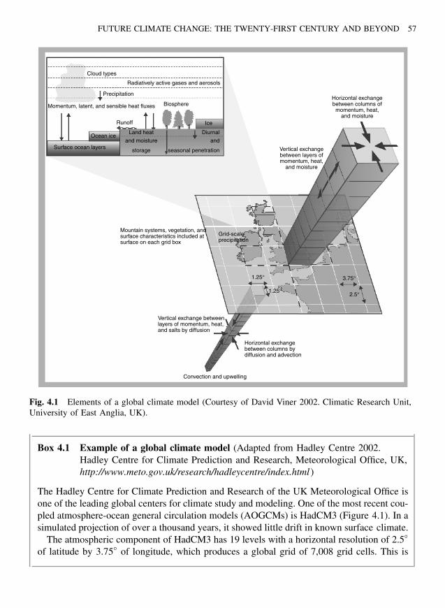
FUTURE CLIMATE CHANGE: THE TWENTY-FIRST CENTURY AND BEYOND 57
Cloud types
Precipitation
Runoff
Radiatively active gases and aerosols
Momentum, latent, and sensible heat fluxes Biosphere
Land heat
and moisture
storage
Ice
Diurnal
and
seasonal penetration
Horizontal exchangebetween columns ofmomentum, heat,
and moisture
Vertical exchangebetween layers ofmomentum, heat,
and moisture
Mountain systems, vegetation, andsurface characteristics included atsurface on each grid box
Vertical exchange betweenlayers of momentum, heat,and salts by diffusion
Grid-scaleprecipitation
1.25° 3.75°
2.5°1.25°
Horizontal exchangebetween columns bydiffusion and advection
Convection and upwelling
Surface ocean layers
Ocean ice
Fig. 4.1 Elements of a global climate model (Courtesy of David Viner 2002. Climatic Research Unit,University of East Anglia, UK).
Box 4.1 Example of a global climate model (Adapted from Hadley Centre 2002.Hadley Centre for Climate Prediction and Research, Meteorological Office, UK,http://www.meto.gov.uk/research/hadleycentre/index.html )
The Hadley Centre for Climate Prediction and Research of the UK Meteorological Office isone of the leading global centers for climate study and modeling. One of the most recent cou-pled atmosphere-ocean general circulation models (AOGCMs) is HadCM3 (Figure 4.1). In asimulated projection of over a thousand years, it showed little drift in known surface climate.
The atmospheric component of HadCM3 has 19 levels with a horizontal resolution of 2.5◦
of latitude by 3.75◦ of longitude, which produces a global grid of 7,008 grid cells. This is
58 CLIMATE CHANGE
equivalent to a surface resolution of about 417 km × 278 km at the equator, reducing to295 km × 278 km at 45◦ of latitude.
A radiation scheme includes six and eight spectral bands in the solar (short wave) andterrestrial thermal (long wave) wavelengths, respectively. The model represents the radiativeeffects of minor greenhouse gases as well as CO2, water vapor, and ozone and also includesa simple parameterization of background aerosol.
A land surface scheme includes a representation of the freezing and melting of soilmoisture, as well as surface runoff and soil drainage; the formulation of evaporation includesthe dependence of stomatal resistance in plant leaves on temperature, vapor pressure, andCO2 concentration. The surface albedo is a function of snow depth, vegetation type, andalso of temperature over snow and ice.
A penetrative convective scheme includes an explicit down-draught and the direct impactof convection on momentum. The large-scale precipitation and cloud scheme is formulated interms of an explicit cloud water variable. The effective radius of cloud droplets is a functionof cloud water content and droplet number concentration. The atmospheric component of themodel also permits the direct and indirect forcing effects of sulfate aerosols to be modeled,given scenarios for sulfur emissions and oxidants.
The oceanic component of HadCM3 has 20 levels with a horizontal resolution of1.25◦ × 1.25◦. At this resolution, it is possible to represent important details in oceaniccurrent structures. Because of its higher ocean resolution, it does not need flux adjustment(additional “artificial” heat and freshwater fluxes at the ocean surface) to produce a goodsimulation. Horizontal mixing is included and horizontal momentum varies with latitude.Regional adjustments in circulation are included in some areas such as the Denmark Straits,and the Iceland–Scotland, and Mediterranean–Atlantic connections.
The sea-ice model uses a simple thermodynamic scheme including snow cover. Thesurface ocean current advects ice, preventing convergence, when the depth exceeds 4 m.There is no explicit representation of iceberg calving, so a prescribed water flux is returnedto the ocean at a rate calibrated to balance the net snowfall accumulation on the ice sheets,geographically distributed within regions where icebergs are found. In order to avoid aglobal average salinity drift, surface water fluxes are converted to surface salinity fluxesusing a constant reference salinity of 35 parts per thousand.
The model is initialized directly from the observed ocean state at rest, with a suitableatmospheric and sea-ice state. The atmosphere and ocean exchange information once perday. Heat and water fluxes are conserved in the transfer between their different grids.
Model simulations can be compared torecent observed climate. Agreement betweenmodeled and observed change depends on therelationship between CO2 concentration andtemperature (temperature sensitivity) assumedin the model. For example, a doublingof CO2 could result in a temperature
increase of as little as 1.5 ◦C or as greatas 4.5 ◦C (Figure 4.2a). Also, correlationbetween observations and model predictionsincreases when the cooling effect of sulfateaerosols is included (Figure 4.2b).
GCMs have evolved and improved overthe past 40 years. Early GCMs treated the

FUTURE CLIMATE CHANGE: THE TWENTY-FIRST CENTURY AND BEYOND 59
0.75
0.50
OBS∆T2x = 1.5°∆T2x = 2.5°∆T2x = 4.5°
OBS∆T2x = 1.5°∆T2x = 2.5°∆T2x = 4.5°
0.25
0.00
−0.25
−0.501850 1880 1910 1940
Time (years)
Tem
pera
ture
ano
mal
y (°
C)
0.75
0.50
0.25
0.00
−0.25
−0.50
Tem
pera
ture
ano
mal
y (°
C)
(a)
1970 2000
1850 1880 1910 1940Time (years)
(b)
1970 2000
Fig. 4.2 Observed (solid line) and simulated global temperature for 2X CO2, dashed lines = threedifferent assumptions of temperature sensitivity to doubling of atmospheric CO2. (a) Model forcing withgreenhouse gases only; (b) greenhouse gases and cooling effect of sulfate aerosols (From IPCC 1996.Climate Change 1995: The Science of Climate Change. Intergovernmental Panel on Climate Change,World Meteorological Organization and United Nations Environment Program. Cambridge: CambridgeUniversity Press, p. 37. Reproduced by permission of Intergovernmental Panel on Climate Change).
ocean heat sink as a static “swamp,” withoutmixing. By 1987, GCMs incorporated clouds,seasonally changing sea ice, and a three-layered ocean with a surface-mixed layer thatserved as the primary heat exchange with theatmosphere (Schlesinger and Mitchell 1987).By 1993 scientists began to look at theimportant ocean component with more sophis-ticated models. A model developed by Albert
Semtner of the US Naval Post GraduateSchool and Robert Chervon of the NCARin the early 1990s divided the ocean intoone-quarter degree blocks and calculated theaverage properties within each. It used eightsupercomputers in parallel, capable of trillionsof calculations per second. Even so, giventhe complexity of the system, it took morethan 100 h of computer time to simulate just

60 CLIMATE CHANGE
one year of detailed ocean circulation. This“Transient Ocean Model” correctly simulatedthe vast looping oceanic conveyer belt cur-rent linking the Pacific, Indian, and AtlanticOceans (see Chapter 1 and Kerr 1993).
Dozens of newer coupled Atmosphere-Ocean General Circulation Models (AOGCMs)have now been developed and assessed. Anaccurate prediction of climate must incorpo-rate not only the physical climate system butthe biosphere as well. For example, the wayin which the biosphere (living matter) reactsto climate change may either dampen or mag-nify climate change. Photosynthesis is a majorsink for atmospheric CO2, the most impor-tant greenhouse gas. Microbes break downorganic matter (e.g. dead vegetation), and theirrelease of CO2 from respiration represents animportant source to the atmosphere. Microor-ganisms are also active in the biogeochemicalcycles of several radiatively important tracegases including methane, sulfur, and nitrogen.Some models now incorporate the interactionsof major biomes, for example, desert, savanna,rain forest, and so on, with the atmosphere(Baskin 1993). Linked climate/biosphere mod-els such as the Dynamic Global Phytogeogra-phy Model of the UK Meteorological Officedemonstrate that predictions of climate changeincluding life may be quite different from, andeven more severe than, climate-change predic-tions in the absence of life.
Several approaches are used to evaluatethe accuracy of climate models. Models aregenerally tested for their ability to simulatethe current global climate including seasonalcycles. They may also be tested to see if theyaccurately “predict” changes that occurredthousands of years ago (Chapter 2) or recenttrends in regional precipitation measured overthe past few decades (Figure 4.3). In gen-eral, most models do a good job in predict-ing atmospheric temperature, precipitation,
surface heat flux, and percent cloudiness. Forexample, 11 different GCMs give similar pre-dictions of mean precipitation patterns in rela-tion to latitude over the globe (Figure 4.4).However, models are less accurate at predict-ing the slow processes of changing ice coveror large-scale ocean circulation.
Feedback Loops and Uncertainties
Any attempt at predicting future conditions willcontain uncertainties. Given the complexity ofthe climate system, it is not surprising thatmodel predictions of global average warmingfor the period 1990 to 2100 range from 1.4to 5.8 ◦C (IPCC 2001). One variable is thatof setting the initial conditions, that is, howmuch anthropogenic change has occurred priorto the initial year of the model run. Also,there are errors in the data against which themodel is compared. For example, models canbe tested for their ability to replicate pastclimates under conditions present long ago, butthe methods used to construct the past climateshave inherent errors of their own.
A feedback is an interaction in which factorsthat produce the result are themselves modifiedby that result. Feedbacks are a common featureof the natural and the human-engineered world.For example, a household thermostat senses theroom temperature. When the room temperaturedrops below the thermostat setting, the thermo-stat triggers the furnace to start. As the roomheats up, the rising temperature, acting as anegative feedback, switches the heat supply offand ends the heating cycle. In a positive feed-back loop, a malfunctioning thermostat wouldrespond to increased temperatures by increas-ing its setting each time a higher temperaturewas reached. Positive feedbacks are of particu-lar concern because of the possible “runaway”behavior they produce. For example, warmingof wetlands could lead to increased microbio-logical activity in the sediments and increased
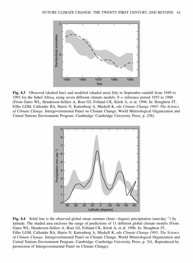
FUTURE CLIMATE CHANGE: THE TWENTY-FIRST CENTURY AND BEYOND 61
2
0
1950 1960 1970Year
Sta
ndar
dize
d an
omal
ies
1980 1990
Fig. 4.3 Observed (dashed line) and modeled (shaded area) July to September rainfall from 1949 to1993 for the Sahel Africa, using seven different climate models. 0 = reference period 1955 to 1988(From Gates WL, Henderson-Sellers A, Boer GJ, Folland CK, Kitoh A, et al. 1996. In: Houghton JT,Filho LGM, Callender BA, Harris N, Kattenberg A, Maskell K, eds Climate Change 1995: The Scienceof Climate Change. Intergovernmental Panel on Climate Change, World Meterological Organization andUnited Nations Environment Program. Cambridge: Cambridge University Press, p. 258).
9
8
7
6
5
4
3
2
1
080 60 40 20 −20 −40 −60 −800
Latitude (degrees)
Pre
cipi
tatio
n (m
m d
ay−1
)
Fig. 4.4 Solid line is the observed global mean summer (June–August) precipitation (mm day−1) bylatitude. The shaded area encloses the range of predictions of 11 different global climate models (FromGates WL, Henderson-Sellers A, Boer GJ, Folland CK, Kitoh A, et al. 1996. In: Houghton JT,Filho LGM, Callender BA, Harris N, Kattenberg A, Maskell K, eds Climate Change 1995: The Scienceof Climate Change. Intergovernmental Panel on Climate Change, World Meterological Organization andUnited Nations Environment Program. Cambridge: Cambridge University Press, p. 241. Reproduced bypermission of Intergovernmental Panel on Climate Change).
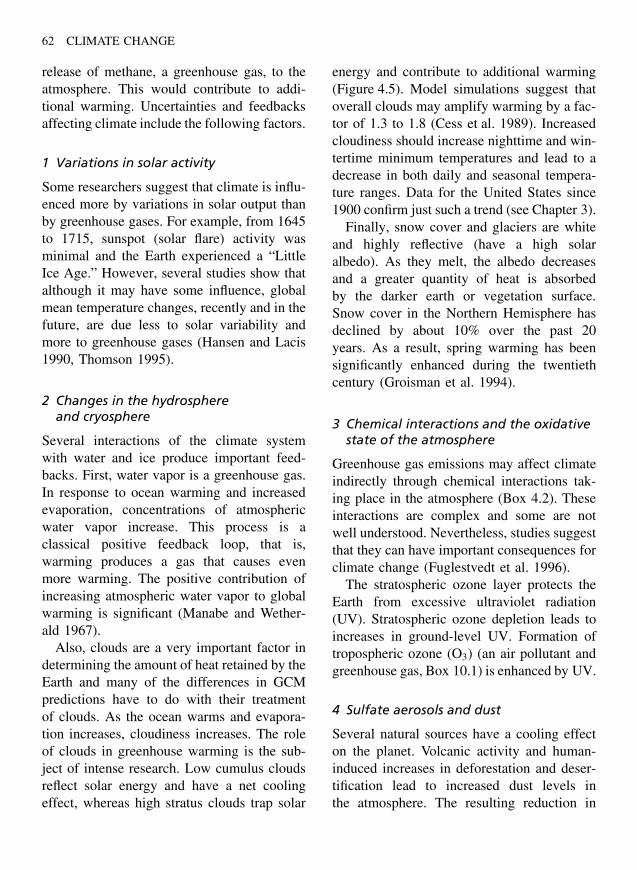
62 CLIMATE CHANGE
release of methane, a greenhouse gas, to theatmosphere. This would contribute to addi-tional warming. Uncertainties and feedbacksaffecting climate include the following factors.
1 Variations in solar activity
Some researchers suggest that climate is influ-enced more by variations in solar output thanby greenhouse gases. For example, from 1645to 1715, sunspot (solar flare) activity wasminimal and the Earth experienced a “LittleIce Age.” However, several studies show thatalthough it may have some influence, globalmean temperature changes, recently and in thefuture, are due less to solar variability andmore to greenhouse gases (Hansen and Lacis1990, Thomson 1995).
2 Changes in the hydrosphereand cryosphere
Several interactions of the climate systemwith water and ice produce important feed-backs. First, water vapor is a greenhouse gas.In response to ocean warming and increasedevaporation, concentrations of atmosphericwater vapor increase. This process is aclassical positive feedback loop, that is,warming produces a gas that causes evenmore warming. The positive contribution ofincreasing atmospheric water vapor to globalwarming is significant (Manabe and Wether-ald 1967).
Also, clouds are a very important factor indetermining the amount of heat retained by theEarth and many of the differences in GCMpredictions have to do with their treatmentof clouds. As the ocean warms and evapora-tion increases, cloudiness increases. The roleof clouds in greenhouse warming is the sub-ject of intense research. Low cumulus cloudsreflect solar energy and have a net coolingeffect, whereas high stratus clouds trap solar
energy and contribute to additional warming(Figure 4.5). Model simulations suggest thatoverall clouds may amplify warming by a fac-tor of 1.3 to 1.8 (Cess et al. 1989). Increasedcloudiness should increase nighttime and win-tertime minimum temperatures and lead to adecrease in both daily and seasonal tempera-ture ranges. Data for the United States since1900 confirm just such a trend (see Chapter 3).
Finally, snow cover and glaciers are whiteand highly reflective (have a high solaralbedo). As they melt, the albedo decreasesand a greater quantity of heat is absorbedby the darker earth or vegetation surface.Snow cover in the Northern Hemisphere hasdeclined by about 10% over the past 20years. As a result, spring warming has beensignificantly enhanced during the twentiethcentury (Groisman et al. 1994).
3 Chemical interactions and the oxidativestate of the atmosphere
Greenhouse gas emissions may affect climateindirectly through chemical interactions tak-ing place in the atmosphere (Box 4.2). Theseinteractions are complex and some are notwell understood. Nevertheless, studies suggestthat they can have important consequences forclimate change (Fuglestvedt et al. 1996).
The stratospheric ozone layer protects theEarth from excessive ultraviolet radiation(UV). Stratospheric ozone depletion leads toincreases in ground-level UV. Formation oftropospheric ozone (O3) (an air pollutant andgreenhouse gas, Box 10.1) is enhanced by UV.
4 Sulfate aerosols and dust
Several natural sources have a cooling effecton the planet. Volcanic activity and human-induced increases in deforestation and deser-tification lead to increased dust levels inthe atmosphere. The resulting reduction in

FUTURE CLIMATE CHANGE: THE TWENTY-FIRST CENTURY AND BEYOND 63
(a)
(b)
Fig. 4.5 (a) Cumulus clouds reflect solar energy back to space and have a cooling effect; (b) cirrusclouds allow solar energy through, but trap heat and have a warming effect. However, how globalwarming will affect clouds and, in turn, the overall radiation balance of the Earth remains one of thelargest uncertainties in global climate modeling.
sunlight reaching the Earth’s surface has acooling effect on climate.
Sulfur comes from both natural and anthro-pogenic sources. Natural sulfur compoundsare emitted by some plankton species in theocean and serve as cloud condensation nuclei(Charlson et al. 1987). Combustion of fos-sil fuel, especially high-sulfur coal, releasessulfur to the atmosphere. Such emissions are
expected to increase atmospheric sulfur by160 to 270% between 1994 and 2040. Inhala-tion of sulfur particles contributes to humanrespiratory illness and is a significant airpollutant causing acid rain and damage toecosystems.
These detrimental effects of atmosphericsulfur are offset to some degree by sulfur’srole in decreasing greenhouse warming. Small
64 CLIMATE CHANGE
Box 4.2 Feedbacks and uncertainties in atmospheric chemistry
Stratospheric ozone depletion increases the formation of hydroxyl radicals (OH−) in theatmosphere.
O3 + UV light −−→ O2 + O
O + H+ −−→ OH−
Reaction with hydroxyl radicals in turn is a primary sink for many gases including CO,CH4, and CFCs, and nonmethane hydrocarbons (NMHC), all of which decrease the oxidationstate of the atmosphere by neutralizing hydroxyl radicals. For example, methane is oxidizedto CO2 (which has only 1/20th of the per molecule warming potential as CH4):
CH4 + 6OH− ←−−→ CO + 5H2O
CO + OH− ←−−→ CO2 + H+
Counterbalancing this removal of OH− could be an increase in OH− from increasing amountsof water vapor in the atmosphere. The net result of these and other chemical interactionsare not well understood.
sulfur particles or aerosols in the atmospherereflect solar energy. In the Northern Hemi-sphere, the negative radiative forcing (cool-ing) due to sulfate aerosols is about equal tothe positive radiative forcing (warming) dueto anthropogenic greenhouse gases (Charlsonet al. 1992, Charlson and Wigley 1994). Thus,the current negative forcing from anthro-pogenic sulfur emissions substantially off-sets global greenhouse warming, especiallyin the Northern Hemisphere (Taylor and Pen-ner 1994, Figure 4.6). Ironically, reductions insulfur emission to improve public health andenvironmental quality will probably exacer-bate global warming.
5 The CO2 fertilization effect
Plants, through photosynthesis, take up CO2
and convert it to organic carbon. Studies, pri-marily in greenhouses, indicate that increasedatmospheric CO2 increases plant growth. Iftrue on a larger scale, this process could
act as a negative feedback on warming,since increased plant biomass would meanmore carbon stored organically rather thanas atmospheric CO2. Since the 1960s, theamplitude of the seasonal atmospheric CO2
variation, that is, low in summer as plantstake up CO2 and high in winter as plants die,has been increasing. This suggests that plantbiomass might indeed be increasing and hav-ing a greater effect on seasonal increases anddecreases in atmospheric CO2.
6 Changes in forest carbon
Forest harvesting releases huge quantities ofstored carbon into the atmosphere. Glob-ally, forests and their soils contain about2,000 billion tonnes (Gt) of carbon. The car-bon storage of the Amazon forest alone isequal to about 30 years of current fossil-fuelcombustion. Trees are converted to lumberand paper – products that store carbon formuch shorter time periods than forests. The
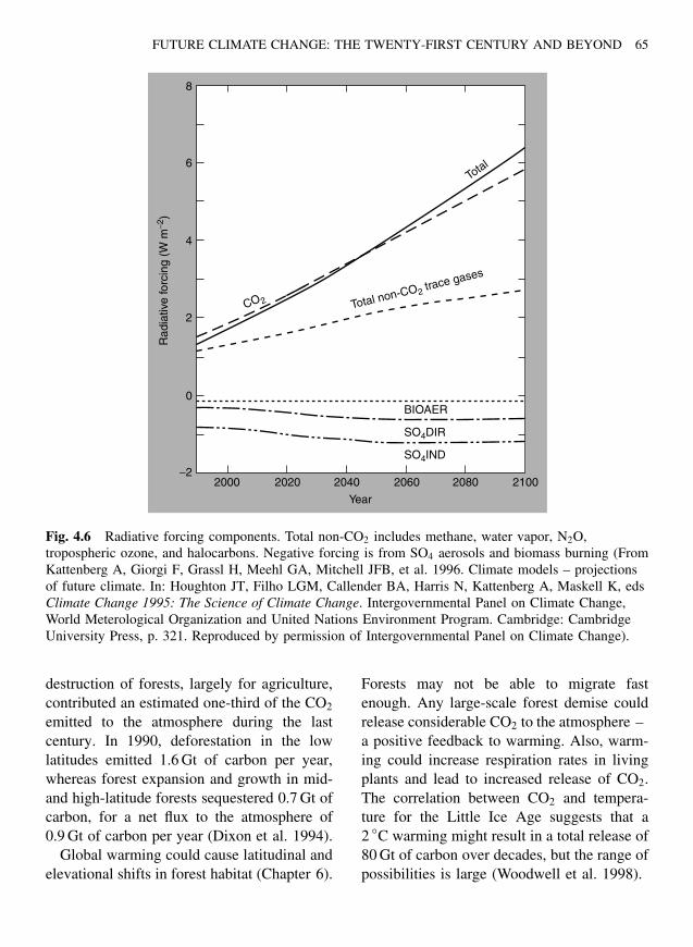
FUTURE CLIMATE CHANGE: THE TWENTY-FIRST CENTURY AND BEYOND 65
8
6
4
CO2
Total
2
0
−22000 2020 2040
Year
Rad
iativ
e fo
rcin
g (W
m−2
)
2060 2080 2100
Total non-CO2 trace gases
BIOAER
SO4DIR
SO4IND
Fig. 4.6 Radiative forcing components. Total non-CO2 includes methane, water vapor, N2O,tropospheric ozone, and halocarbons. Negative forcing is from SO4 aerosols and biomass burning (FromKattenberg A, Giorgi F, Grassl H, Meehl GA, Mitchell JFB, et al. 1996. Climate models – projectionsof future climate. In: Houghton JT, Filho LGM, Callender BA, Harris N, Kattenberg A, Maskell K, edsClimate Change 1995: The Science of Climate Change. Intergovernmental Panel on Climate Change,World Meterological Organization and United Nations Environment Program. Cambridge: CambridgeUniversity Press, p. 321. Reproduced by permission of Intergovernmental Panel on Climate Change).
destruction of forests, largely for agriculture,contributed an estimated one-third of the CO2
emitted to the atmosphere during the lastcentury. In 1990, deforestation in the lowlatitudes emitted 1.6 Gt of carbon per year,whereas forest expansion and growth in mid-and high-latitude forests sequestered 0.7 Gt ofcarbon, for a net flux to the atmosphere of0.9 Gt of carbon per year (Dixon et al. 1994).
Global warming could cause latitudinal andelevational shifts in forest habitat (Chapter 6).
Forests may not be able to migrate fastenough. Any large-scale forest demise couldrelease considerable CO2 to the atmosphere –a positive feedback to warming. Also, warm-ing could increase respiration rates in livingplants and lead to increased release of CO2.The correlation between CO2 and tempera-ture for the Little Ice Age suggests that a2 ◦C warming might result in a total release of80 Gt of carbon over decades, but the range ofpossibilities is large (Woodwell et al. 1998).
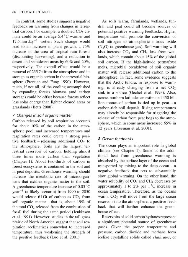
66 CLIMATE CHANGE
In contrast, some studies suggest a negativefeedback on warming from changes in terres-trial carbon. For example, a doubled CO2 cli-mate could be an average 5.4 ◦C warmer and17.5 mm day−1 wetter. Such change wouldlead to an increase in plant growth, a 75%increase in the area of tropical rain forests(discounting harvesting), and a reduction indesert and semidesert areas by 60% and 20%,respectively. The overall effect would be aremoval of 235 Gt from the atmosphere and itsstorage as organic carbon in the terrestrial bio-sphere (Prentice and Fung 1990). However,much, if not all, of the cooling accomplishedby expanding forests biomass (and carbonstorage) could be offset because forests reflectless solar energy than lighter cleared areas orgrasslands (Betts 2000).
7 Changes in soil organic matterCarbon released by soil respiration accountsfor about 10% of the carbon in the atmo-spheric pool, and increased temperatures andrespiration rates could create a strong posi-tive feedback – releasing additional CO2 tothe atmosphere. Soils are the largest ter-restrial reservoir of carbon, holding almostthree times more carbon than vegetation(Chapter 1). About two-thirds of carbon inforest ecosystems is contained in the soil andin peat deposits. Greenhouse warming shouldincrease the metabolic rate of microorgan-isms that oxidize organic matter in the soil.A greenhouse temperature increase of 0.03 ◦Cyear−1 (a likely scenario) from 1990 to 2050would release 61 Gt of carbon as CO2 fromsoil organic matter – that is, about 19% ofthe total CO2 released from the combustion offossil fuel during the same period (Jenkinsonet al. 1991). However, studies in the tall grassprairie of North America suggest that soil res-piration acclimatizes somewhat to increasedtemperature, thus weakening the strength ofthe positive feedback (Luo et al. 2001).
As soils warm, farmlands, wetlands, tun-dra, and peat could all become sources ofpotential positive warming feedbacks. Highertemperature will promote the conversion ofsoil nitrogen to atmospheric nitrous oxide(N2O) (a greenhouse gas). Soil warming willalso increase CO2 and CH4 loss from wet-lands, which contain about 15% of the globalsoil carbon. If the high-latitude permafrostmelts, microbial breakdown of soil organicmatter will release additional carbon to theatmosphere. In fact, some evidence suggeststhat the Arctic tundra, in response to warm-ing, is already changing from a net CO2
sink to a source (Oechel et al. 1993). Also,across northern latitudes an estimated 450 bil-lion tonnes of carbon is tied up in peat – acarbon-rich soil deposit. Rising temperaturesmay already be responsible for triggering therelease of carbon from peat bogs to the atmo-sphere, which in some areas increased 65% in12 years (Freeman et al. 2001).
8 Ocean feedbacks
The ocean plays an important role in globalclimate (see Chapter 1). Some of the addi-tional heat from greenhouse warming isabsorbed by the surface layer of the ocean andtransported by mixing to the deep ocean – anegative feedback that acts to substantiallyslow global warming. On the other hand, thewater solubility of CO2 and CH4 decreases byapproximately 1 to 2% per 1 ◦C increase inocean temperature. Therefore, as the oceanswarm, CO2 will move from the large oceanreservoir into the atmosphere, a positive feed-back that will further enhance the green-house effect.
Reservoirs of solid carbon hydrates representa significant potential source of greenhousegases. Given the proper temperature andpressure, carbon dioxide and methane formicelike crystalline solids called clathrates, or

FUTURE CLIMATE CHANGE: THE TWENTY-FIRST CENTURY AND BEYOND 67
gas hydrates. These forms of carbon occur insome shallow sea sediments and tundra. Warm-ing could melt these clathrates, releasing largequantities of methane or carbon dioxide intothe water column and from there into the atmo-sphere, increasing global warming (Wilde andQuinby-Hunt 1997).
Studies using a coupled ocean-atmospheremodel suggest that increased rainfall fromgreenhouse warming will result in surfacefreshening (decreased density) and stratifica-tion of seawater over a large area of theSouthern Ocean. The decrease in downwardmixing and transport of heat and carbon tothe deep ocean could substantially decreasethe oceanic uptake of CO2 over the next fewdecades (Sarmiento et al. 1998).
9 Overall climate carbon cycle feedbacks
At least one study linking a carbon cycle modelto an AOGCM suggests that global warmingwill reduce both terrestrial and oceanic uptakeof CO2. Net ecosystem productivity (carbonstorage) will be strongly reduced in the sub-tropics by increases in soil aridity. At thesame time, three factors will reduce oceanicuptake of carbon, especially at high latitudes:(1) decreased solubility of CO2 at higher tem-peratures, (2) increased density stratificationwith warm waters lying on the surface thatreduce vertical mixing and transport of CO2 tothe deep ocean, and (3) changes in the biogeo-chemical cycle of CO2. The gain in atmosphericCO2 from these feedbacks is 10% with a dou-bled and 20% with a quadrupled CO2 atmo-sphere. This translates into a 15% higher meanglobal temperature increase than would occurin the absence of these feedbacks (Friedling-stein et al. 2001).
10 The human dimension
Perhaps the greatest sources of uncertainty inpredicting future climate change arise from
the human dimension (Chapters 9 to 12).Future greenhouse gas emissions depend onhuman population and economic growth, andper capita emissions. New technologies mightdirectly reduce or sequester greenhouse gasemissions from fossil-fuel combustion. Con-tinued increases in energy efficiency and useof alternative (nonfossil fuel) energy couldreduce emission growth rates. Mitigation andadaptation could, in a variety of ways, offsetthe negative impacts of climate change. Con-tinuing attempts at international agreementscould fail or could succeed in greatly reducinggreenhouse gas emissions.
Scenario-Based Climate Predictions
Despite the complexity of the Earth-climatesystem and the uncertainties involved in mod-eling, our ability to predict the climatic effectsof greenhouse gas emissions continues toimprove. New models consider the effectsof sulfate aerosol cooling, of changes in theEarth’s albedo due to melting ice, and thechanges in atmospheric trace gas concentra-tions other than CO2. The ability to “predict”changes that already occurred during the twen-tieth century or earlier has led to improvedconfidence in these models. Nevertheless, mod-els often differ significantly in their predictedoutputs. The Intergovernmental Panel on Cli-mate Change (IPCC), to encompass the rangeof uncertainty in predicted changes, collectedresults from numerous models incorporatingtransient increases in greenhouse gases. Moststudies assume a 1% per year increase in atmo-spheric greenhouse gas concentrations untilCO2 doubling, tripling, or quadrupling. In addi-tion, the IPCC developed a series of emissionscenarios (SRES) to encompass possible rangesof future human population and economicgrowth that influence fossil-fuel consumption(Box 4.3).
68 CLIMATE CHANGE
Box 4.3 Emission scenarios (SRES)
In earlier studies, the IPCC used a set of scenarios called IS92 for a range of futureeconomic and population assumptions. For example, IS92a, often called the business asusual scenario, assumes continuation of current rates of population and economic growth.Following 1996, the IPCC developed a set of 40 new scenarios covering a wide rangeof possible future demographic, economic, and technological forces that influence futuregreenhouse gas and aerosol emissions. In the Special Report on Emission Scenarios (SRES),each scenario represents a specific quantification of four primary “storylines.” However, forillustrative purposes, six Illustrative Marker Scenarios are most often cited (A1B, A1T,A1FI, A2, B1, and B2). Detailed definitions and references to these scenarios can be foundin IPCC (2001).A1. The A1 storyline and scenario family describes a future world of very rapid economicgrowth, global population that peaks in midcentury and declines thereafter, and therapid introduction of new and more efficient technologies. Major underlying themes areconvergence among regions, infrastructure capacity building, and increased cultural andsocial interactions, with substantial reduction in regional differences in per capita income.The A1 scenario family develops into three groups that describe alternative directionsof technological change in the energy system. The three A1 groups are distinguished bytheir technological emphasis: fossil-intensive (A1FI), nonfossil energy sources (A1T), or abalance across all sources (A1B) (where balance is defined as not relying too heavily onone particular energy source, on the assumption that similar improvement rates apply to allenergy supply and end-use technologies).
A2. The A2 storyline and scenario family describe a very heterogeneous world. Theunderlying theme is self-reliance and preservation of local identities. Fertility patternsacross regions converge very slowly, which results in continuously increasing populations.Economic development is primarily region-oriented, and per capita economic growth andtechnological change are more fragmented and slower than in other storylines.
B1. The B1 storyline and scenario family describes a convergent world with thesame global population that peaks in midcentury and declines thereafter, as in the A1storyline, but with rapid change in economic structures toward a service and informationeconomy, with reduction in material intensity and the introduction of clean and resource-efficient technologies. The emphasis is on global solutions to economic, social, andenvironmental sustainability, including improved equity, but without additional climateinitiatives.
B2. The B2 storyline and scenario family describe a world in which the emphasis is onlocal solutions to economic, social, and environmental sustainability. It is a world withcontinuously increasing global population, at a rate lower than A2, intermediate levels ofeconomic development, and less rapid and more diverse technological change than in theB1 and A1 storylines. While the scenario is also oriented toward environmental protectionand social equity, it focuses on local and regional levels.
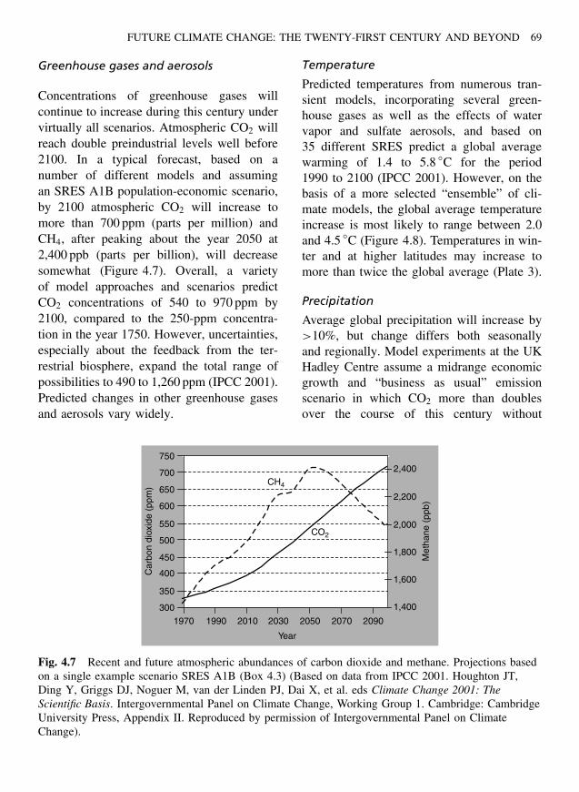
FUTURE CLIMATE CHANGE: THE TWENTY-FIRST CENTURY AND BEYOND 69
Greenhouse gases and aerosols
Concentrations of greenhouse gases willcontinue to increase during this century undervirtually all scenarios. Atmospheric CO2 willreach double preindustrial levels well before2100. In a typical forecast, based on anumber of different models and assumingan SRES A1B population-economic scenario,by 2100 atmospheric CO2 will increase tomore than 700 ppm (parts per million) andCH4, after peaking about the year 2050 at2,400 ppb (parts per billion), will decreasesomewhat (Figure 4.7). Overall, a varietyof model approaches and scenarios predictCO2 concentrations of 540 to 970 ppm by2100, compared to the 250-ppm concentra-tion in the year 1750. However, uncertainties,especially about the feedback from the ter-restrial biosphere, expand the total range ofpossibilities to 490 to 1,260 ppm (IPCC 2001).Predicted changes in other greenhouse gasesand aerosols vary widely.
Temperature
Predicted temperatures from numerous tran-sient models, incorporating several green-house gases as well as the effects of watervapor and sulfate aerosols, and based on35 different SRES predict a global averagewarming of 1.4 to 5.8 ◦C for the period1990 to 2100 (IPCC 2001). However, on thebasis of a more selected “ensemble” of cli-mate models, the global average temperatureincrease is most likely to range between 2.0and 4.5 ◦C (Figure 4.8). Temperatures in win-ter and at higher latitudes may increase tomore than twice the global average (Plate 3).
Precipitation
Average global precipitation will increase by>10%, but change differs both seasonallyand regionally. Model experiments at the UKHadley Centre assume a midrange economicgrowth and “business as usual” emissionscenario in which CO2 more than doublesover the course of this century without
750
700
650
600
550
500
450
400
350
300
1970 1990 2010 2030
Year
Car
bon
diox
ide
(ppm
)
Met
hane
(pp
b)
2050 2070 2090
1,400
1,600
1,800
2,000
2,200
2,400CH4
CO2
Fig. 4.7 Recent and future atmospheric abundances of carbon dioxide and methane. Projections basedon a single example scenario SRES A1B (Box 4.3) (Based on data from IPCC 2001. Houghton JT,Ding Y, Griggs DJ, Noguer M, van der Linden PJ, Dai X, et al. eds Climate Change 2001: TheScientific Basis. Intergovernmental Panel on Climate Change, Working Group 1. Cambridge: CambridgeUniversity Press, Appendix II. Reproduced by permission of Intergovernmental Panel on ClimateChange).
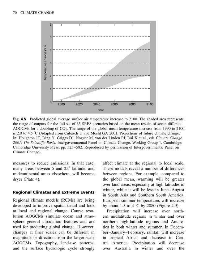
70 CLIMATE CHANGE
6
5
4
3
2
1
02000 2020 2040
Year
Tem
pera
ture
cha
nge
(°C
)
2060 2080 2100
Fig. 4.8 Predicted global average surface air temperature increase to 2100. The shaded area representsthe range of outputs for the full set of 35 SRES scenarios based on the mean results of seven differentAOGCMs for a doubling of CO2. The range of the global mean temperature increase from 1990 to 2100is 2.0 to 4.5 ◦C (Adapted from Cubasch U and Meehl GA 2001. Projections of future climate change.In: Houghton JT, Ding Y, Griggs DJ, Noguer M, van der Linden PJ, Dai X et al., eds Climate Change2001: The Scientific Basis. Intergovernmental Panel on Climate Change, Working Group 1. Cambridge:Cambridge University Press, pp. 525–582. Reproduced by permission of Intergovernmental Panel onClimate Change).
measures to reduce emissions. In that case,many areas between 5 and 25◦ latitude, andmidcontinental areas elsewhere, will becomedryer (Plate 4).
Regional Climates and Extreme Events
Regional climate models (RCMs) are beingdeveloped to improve spatial detail and lookat local and regional change. Course reso-lution AOGCMs simulate ocean and atmo-sphere general circulation features and areused for predicting global change. However,changes at finer scales can be different inmagnitude or direction from the larger-scaleAOGCMs. Topography, land-use patterns,and the surface hydrologic cycle strongly
affect climate at the regional to local scale.These models reveal a number of differencesbetween regions. For example, compared tothe global mean, warming will be greaterover land areas, especially at high latitudes inwinter, while it will be less in June–Augustin South Asia and Southern South America.European summer temperatures will increaseby about 1.5 to 4 ◦C by 2080 (Figure 4.9).
Precipitation will increase over north-ern midlatitude regions in winter and overnorthern high-latitude regions and Antarc-tica in both winter and summer. In Decem-ber–January–February, rainfall will increasein tropical Africa and decrease in Cen-tral America. Precipitation will decreaseover Australia in winter and over the
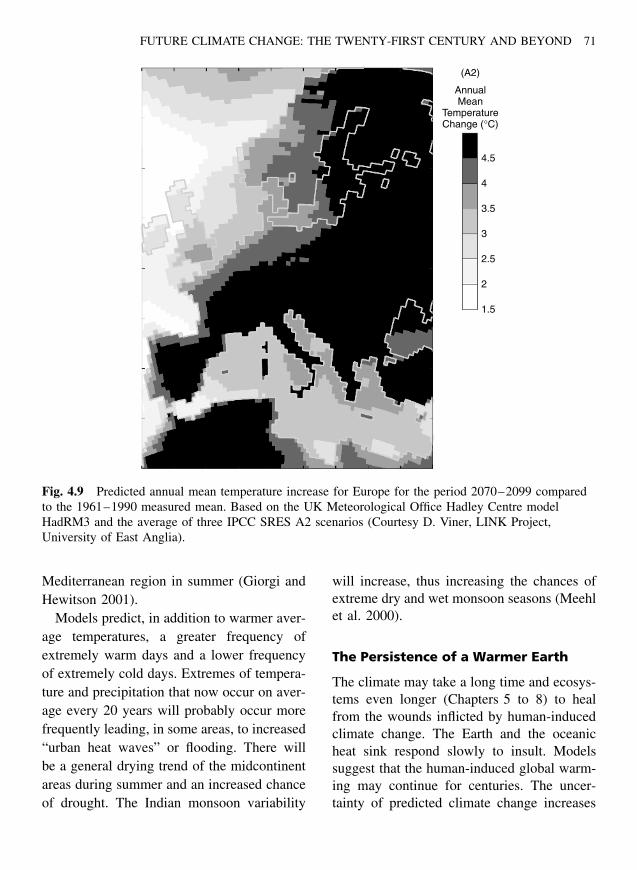
FUTURE CLIMATE CHANGE: THE TWENTY-FIRST CENTURY AND BEYOND 71
(A2)
1.5
2
2.5
3
3.5
4
4.5
AnnualMean
TemperatureChange (°C)
Fig. 4.9 Predicted annual mean temperature increase for Europe for the period 2070–2099 comparedto the 1961–1990 measured mean. Based on the UK Meteorological Office Hadley Centre modelHadRM3 and the average of three IPCC SRES A2 scenarios (Courtesy D. Viner, LINK Project,University of East Anglia).
Mediterranean region in summer (Giorgi andHewitson 2001).
Models predict, in addition to warmer aver-age temperatures, a greater frequency ofextremely warm days and a lower frequencyof extremely cold days. Extremes of tempera-ture and precipitation that now occur on aver-age every 20 years will probably occur morefrequently leading, in some areas, to increased“urban heat waves” or flooding. There willbe a general drying trend of the midcontinentareas during summer and an increased chanceof drought. The Indian monsoon variability
will increase, thus increasing the chances ofextreme dry and wet monsoon seasons (Meehlet al. 2000).
The Persistence of a Warmer Earth
The climate may take a long time and ecosys-tems even longer (Chapters 5 to 8) to healfrom the wounds inflicted by human-inducedclimate change. The Earth and the oceanicheat sink respond slowly to insult. Modelssuggest that the human-induced global warm-ing may continue for centuries. The uncer-tainty of predicted climate change increases
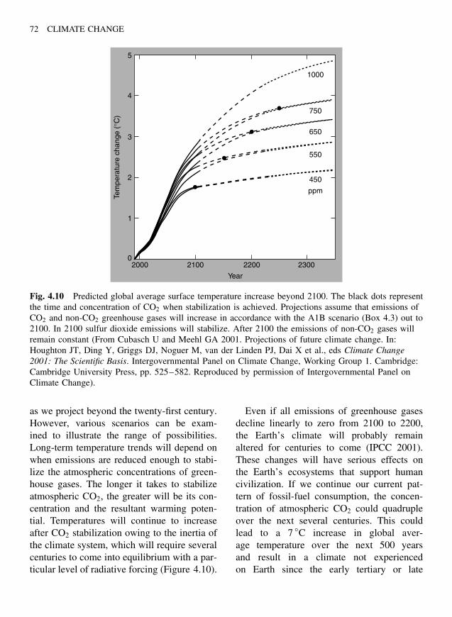
72 CLIMATE CHANGE
5
4
3
2
1
02000 2100 2200
Year
Tem
pera
ture
cha
nge
(°C
)
2300
1000
750
650
550
450
ppm
Fig. 4.10 Predicted global average surface temperature increase beyond 2100. The black dots representthe time and concentration of CO2 when stabilization is achieved. Projections assume that emissions ofCO2 and non-CO2 greenhouse gases will increase in accordance with the A1B scenario (Box 4.3) out to2100. In 2100 sulfur dioxide emissions will stabilize. After 2100 the emissions of non-CO2 gases willremain constant (From Cubasch U and Meehl GA 2001. Projections of future climate change. In:Houghton JT, Ding Y, Griggs DJ, Noguer M, van der Linden PJ, Dai X et al., eds Climate Change2001: The Scientific Basis. Intergovernmental Panel on Climate Change, Working Group 1. Cambridge:Cambridge University Press, pp. 525–582. Reproduced by permission of Intergovernmental Panel onClimate Change).
as we project beyond the twenty-first century.However, various scenarios can be exam-ined to illustrate the range of possibilities.Long-term temperature trends will depend onwhen emissions are reduced enough to stabi-lize the atmospheric concentrations of green-house gases. The longer it takes to stabilizeatmospheric CO2, the greater will be its con-centration and the resultant warming poten-tial. Temperatures will continue to increaseafter CO2 stabilization owing to the inertia ofthe climate system, which will require severalcenturies to come into equilibrium with a par-ticular level of radiative forcing (Figure 4.10).
Even if all emissions of greenhouse gasesdecline linearly to zero from 2100 to 2200,the Earth’s climate will probably remainaltered for centuries to come (IPCC 2001).These changes will have serious effects onthe Earth’s ecosystems that support humancivilization. If we continue our current pat-tern of fossil-fuel consumption, the concen-tration of atmospheric CO2 could quadrupleover the next several centuries. This couldlead to a 7 ◦C increase in global aver-age temperature over the next 500 yearsand result in a climate not experiencedon Earth since the early tertiary or late
FUTURE CLIMATE CHANGE: THE TWENTY-FIRST CENTURY AND BEYOND 73
Cretaceous period – over 140,000 years ago(Manabe 1998).
Summary
The science of climate prediction has im-proved immensely during the past few decades.New and more refined models, incorporatingmany of the known feedbacks, indicate thatthe climate is already warming in responseto anthropogenic emissions of greenhousegases. Furthermore, changes in temperatureand precipitation patterns will continue andaccelerate during this century and possibly forcenturies to come. Several important uncer-tainties in the current numerical models frus-trate predictions of climate. Chief among theseis the prediction of human behavior. How willhuman population growth, economic change,and improvements in technology alter our con-sumption of fossil fuel? Despite the uncertain-ties, policy decisions to deal with fossil-fuelemissions must be made (see Chapter 12). Wecould decide to reduce emissions immediatelyas an insurance policy against future damage.On the other hand, we could wait until predic-tions are even more certain, delaying immedi-ate costs of emissions reductions, but riskingthe possibility of environmental catastrophe.Our choice will be critical in determining thefuture health of the Earth’s ecosystems and thehuman population.
References
Arrhenius S 1896 On the influence of carbonic acidin the air upon the temperature of the ground.Philosophical Magazine and Journal of Science.Series 5 41(251): 237–276.
Baskin Y 1993 Ecologists put some life into modelsof a changing world. Science 259: 1694–1696.
Betts RA 2000 Offset of the potential carbon sinkfrom boreal forestation by decreases in surfacealbedo. Nature 408: 187–190.
Cess RD, Potter GL, Blanchet JP, Boer GJ, Ghan SJ,Kiehl JT, et al. 1989 Interpretation of cloud-climate feedback as produced by 14 atmosphericcirculation models. Science 245: 513–516.
Charlson RJ, Lovelock JE, Andreae MO and War-ren SG 1987 Oceanic phytoplankton, atmo-spheric sulphur, cloud albedo and climate. Nature326(6114): 655–661.
Charlson RJ, Schwartz SE, Hales JM, Cess RD,Coakley Jr JA, Hansen JE, et al. 1992 Climateforcing by anthropogenic aerosols. Science 255:423–430.
Charlson RJ and Wigley TML 1994 Sulfate aerosoland climatic change. Scientific American Febru-ary: 48–57.
Cubasch U and Meehl GA 2001 Projections offuture climate change. In: Houghton JT, Ding Y,Griggs DJ, Noguer M, van der Linden PJ, Dai X,et al. eds Climate Change 2001: The Scien-tific Basis . Intergovernmental Panel on ClimateChange, Working Group 1. Cambridge: CambridgeUniversity Press, pp. 525–582.
Dixon RK, Brown S, Houghton RA, Solomon AM,Trexler MC and Wisniewski J 1994 Carbon poolsand flux of global forest ecosystems. Science 263:185–190.
Freeman C, Evans CD, Monteith DT, Reynolds Band Fenner N 2001 Export of organic carbon frompeat soils. Nature 412: 785.
Friedlingstein P, Fairhead L, LeTreut H, Monfray Pand Orr J 2001 Positive feedback between futureclimate change and the carbon cycle. GeophysicalResearch Letters 28(8): 1543–1546.
Fuglestvedt JS, Isaksen ISA and Wang WC 1996Estimates of indirect global warming potentialsfor CH4, CO and NOX. Climatic Change 34:405–437.
Gates WL, Henderson-Sellers A, Boer GJ, FollandCK, Kitoh A, et al. 1996 In: Houghton JT, FilhoLGM, Callender BA, Harris N, Kattenberg A,Maskell K, eds Climate Change 1995: TheScience of Climate Change. IntergovernmentalPanel on Climate Change, World MeterologicalOrganization and United Nations EnvironmentProgram. Cambridge: Cambridge University Press,pp. 228–284.
Giorgi F and Hewitson B 2001 Regional cli-mate information – evaluation and projections. In:Houghton JT, Ding Y, Griggs DJ, Noguer M, vander Linden PJ, Dai X, et al. eds Climate Change2001: The Scientific Basis . Intergovernmental
74 CLIMATE CHANGE
Panel on Climate Change, Working Group 1. Cam-bridge: Cambridge University Press, pp. 583–638.
Groisman PY, Karl TR and Knight RW 1994Observed impact of snow cover on the heat balanceand the rise of spring continental temperatures.Science 263: 198–200.
Hadley Centre 2002 Hadley Centre for Climate Pre-diction and Research , UK: Meteorological Office,http://www.meto.gov.uk/research/hadleycentre/index.html .
Hansen JE and Lacis AA 1990 Sun and dust versusthe greenhouse gases: an assessment of theirrelative roles in global climate change. Nature 346:713–719.
Hulme M and Carter TR 2000 The changing climateof Europe. In: Parry ML, ed. Assessment of Poten-tial Effects and Adaptations for Climate Change inEurope: The Europe ACACIA Project . Norwich,UK: The Jackson Environment Institute, UEA,pp. 47–84.
IPCC 1996 Climate Change 1995: The Science of Cli-mate Change. Intergovernmental Panel on ClimateChange, World Meteorological Organization andUnited Nations Environment Program. Cambridge:Cambridge University Press, p. 37.
IPCC 2001 Houghton JT, Ding Y, Griggs DJ, NoguerM, van der Linden PJ, Dai X, et al. eds Cli-mate Change 2001: The Scientific Basis . Inter-governmental Panel on Climate Change, Work-ing Group 1. Cambridge: Cambridge UniversityPress.
Jenkinson DS, Adams DE and Wild A 1991 Modelestimates of CO2 emissions from soil in responseto global warming. Nature 361: 304–306.
Kattenberg A, Giorgi F, Grassl H, Meehl GA,Mitchell JFB, et al. 1996 Climate models –projections of future climate. In: Houghton JT,Filho LGM, Callender BA, Harris N, Katten-berg A, Maskell K, eds Climate Change 1995:The Science of Climate Change. Intergovernmen-tal Panel on Climate Change, World Meterologi-cal Organization and United Nations EnvironmentProgram. Cambridge: Cambridge University Press,pp. 285–357.
Kerr RA 1993 Ocean-in-a-machine starts looking likethe real thing. Science 260: 32,33.
Luo Y, Wan S, Hui D and Wallace LL 2001 Acclimatization of soil respiration to warming in a tallgrass prairie. Nature 413: 622–624.
Manabe S 1998 Study of global warming by GFDLclimate models. Ambio 27(3): 182–186.
Manabe S and Wetherald RT 1967 Thermal equilib-rium of the atmosphere with a given distributionof relative humidity. Journal of the AtmosphericSciences 24: 241–259.
Meehl GA, Zwiers F, Evans J, Knutson T, Mearns Land Whetton P 2000 Trends in extreme weatherand climate events: issues related to modelingextremes in projections of future climatic change.Bulletin of the American Meteorological Society81(3): 427–436.
Oechel WC, Hastings SJ, Vourlitis G, Jenkins M,Riechers G and Grulke N 1993 Recent evidence ofArctic tundra ecosystems from a net carbon dioxidesink to a source. Science 361: 520–523.
Prentice K and Fung IY 1990 The sensitivity of car-bon storage to climate change. Nature 346: 48–51.
Sarmiento JL, Hughes TMC, Stouffer RJ and Man-abe S 1998 Simulated response of the ocean car-bon cycle to anthropogenic warming. Nature 393:245–249.
Schlesinger ME and Mitchell JFB 1987 Climatemodel simulations of the equilibrium climaticresponse to increased carbon dioxide. Reviews ofGeophysics 25: 760–798.
Taylor KE and Penner JE 1994 Response of the cli-mate system to atmospheric aerosols and green-house gases. Nature 369: 734–737.
Thomson DJ 1995 The seasons, global temperature,and precession. Science 268: 59–69.
Viner D 2002 Elements of a Global Climate Model .Norwich, UK: Climatic Research Unit, Universityof East Anglia, http://www.cru. uea.ac.uk/cru/info/modelcc/.
Wilde P and Quinby-Hunt MS 1997 Methane clathrateoutgassing and anoxic expansion in southeast Asiandeeps due to global warming. Environmental Mon-itoring and Assessment 44: 149–153.
Woodwell GM, MacKensie FT, Houghton RA,Apps M, Gorham E and Davidson E 1998 Bioticfeedbacks in the warming of the Earth. ClimaticChange 40: 495–518.

SECTION II
Ecological Effects of Climate Change
75

This Page Intentionally Left Blank
Chapter 5
Effects onFreshwater Systems
“A greenhouse warming is certain to have major impactson both water availability and water quality.”
Kenneth Frederick and Peter Gleick
Introduction
Climate-induced changes in precipitation, sur-face runoff, and soil moisture will probablyhave profound impacts on natural systemsand human populations. Life on land, instreams, and in lakes depends on the avail-ability of freshwater. Globally, precipita-tion averages about 86 cm (34 inches) peryear, and ranges from 25 to 254 cm (10 to100 inches) per year over most of the world.These differences in precipitation patterns,along with temperature, largely determinethe geographic distribution of major terres-trial ecosystems (biomes) from deserts torain forests (Chapter 6). Surface and ground-water sources supply water to humans fordomestic use, agricultural irrigation, indus-try, transportation, recreation, waste disposal,and hydroelectric power generation. Humansettlements have been, and continue to be,linked closely to the availability of freshwa-ter. In fact, many historians believe successful
early agricultural civilizations such as those inAfrica (Egypt) or Central America (Mayan)developed out of the social organizationnecessary for large-scale water-managementprojects. Today, about 1.7 billion people orone-third of the world’s population live inareas of water scarcity, that is, where theyuse more than 20% of their renewable watersupply. This number is projected to grow,depending on population growth rates, toabout 5 billion by 2025.
Because of the basic importance of waterto living systems, changes in water availabil-ity represent one of the most serious poten-tial consequences of greenhouse warming.Global warming could create new challengesfor areas already facing water supply prob-lems. Warming will accelerate oceanic evap-oration and increase overall global averageprecipitation. On the basis of the SRES A2scenario (see Chapter 4), the 30-year aver-age precipitation for the period 2071 to 2100will be 3.9% (range = 1.3 to 6.8%) greater
Climate Change: Causes, Effects, and Solutions John T. Hardy 2003 John Wiley & Sons, Ltd ISBNs: 0-470-85018-3 (HB); 0-470-85019-1 (PB)
77
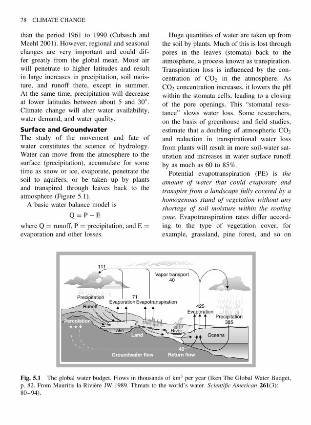
78 CLIMATE CHANGE
than the period 1961 to 1990 (Cubasch andMeehl 2001). However, regional and seasonalchanges are very important and could dif-fer greatly from the global mean. Moist airwill penetrate to higher latitudes and resultin large increases in precipitation, soil mois-ture, and runoff there, except in summer.At the same time, precipitation will decreaseat lower latitudes between about 5 and 30◦.Climate change will alter water availability,water demand, and water quality.
Surface and GroundwaterThe study of the movement and fate ofwater constitutes the science of hydrology.Water can move from the atmosphere to thesurface (precipitation), accumulate for sometime as snow or ice, evaporate, penetrate thesoil to aquifers, or be taken up by plantsand transpired through leaves back to theatmosphere (Figure 5.1).
A basic water balance model is
Q = P − E
where Q = runoff, P = precipitation, and E =evaporation and other losses.
Huge quantities of water are taken up fromthe soil by plants. Much of this is lost throughpores in the leaves (stomata) back to theatmosphere, a process known as transpiration.Transpiration loss is influenced by the con-centration of CO2 in the atmosphere. AsCO2 concentration increases, it lowers the pHwithin the stomata cells, leading to a closingof the pore openings. This “stomatal resis-tance” slows water loss. Some researchers,on the basis of greenhouse and field studies,estimate that a doubling of atmospheric CO2
and reduction in transpirational water lossfrom plants will result in more soil-water sat-uration and increases in water surface runoffby as much as 60 to 85%.
Potential evapotranspiration (PE) is theamount of water that could evaporate andtranspire from a landscape fully covered by ahomogenous stand of vegetation without anyshortage of soil moisture within the rootingzone. Evapotranspiration rates differ accord-ing to the type of vegetation cover, forexample, grassland, pine forest, and so on
111
71Evaporation Evapotranspiration
Vapor transport40
Precipitation
Runoff
Lake River
Percolation
Land
Groundwater flow40
Return flow
425Evaporation
Precipitation385
Oceans
Fig. 5.1 The global water budget. Flows in thousands of km3 per year (Iken The Global Water Budget,p. 82. From Mauritis la Riviere JW 1989. Threats to the world’s water. Scientific American 261(3):80–94).
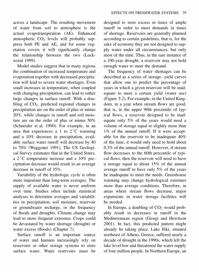
EFFECTS ON FRESHWATER SYSTEMS 79
across a landscape. The resulting movementof water from soil to atmosphere is theactual evapotranspiration (AE). Enhancedatmospheric CO2 levels will probably sup-press both PE and AE, and for some veg-etation covers it will significantly changethe relationship between the two (Lock-wood 1999).
Model studies suggest that in many regionsthe combination of increased temperature andevaporation together with decreased precipita-tion will lead to severe water shortages. Evensmall increases in temperature, when coupledwith changing precipitation, can lead to ratherlarge changes in surface runoff. With a dou-bling of CO2, predicted regional changes inprecipitation are on the order of plus or minus20%, while changes in runoff and soil mois-ture are on the order of plus or minus 50%(Schneider et al. 1990). For example, in anarea that experiences a 1 to 2 ◦C warmingand a 10% decrease in precipitation, avail-able surface water runoff will decrease by 40to 70% (Waggoner 1991). The US Geologi-cal Survey estimates that in the United States,a 2 ◦C temperature increase and a 10% pre-cipitation decrease would result in an averagedecrease in runoff of 35%.
Variability of the hydrologic cycle is oftenmore important than long-term averages. Thesupply of available water is never uniformover time. Studies often include statisticalanalyses to determine averages and variabili-ties in precipitation, soil moisture, reservoiror groundwater recharge, or the frequencyof floods and droughts. Climate change maylead to more frequent extremes. Crops couldbe devastated by water shortage (drought) orwater excess (floods) (Chapter 7).
Surface runoff is an important sourceof water and humans increasingly rely onreservoirs or other storage systems to storesurface water. Water reservoirs must be
designed to store excess in times of amplerunoff in order to meet demands in timesof shortage. Reservoirs are generally plannedaccording to certain guidelines, that is, for thesake of economy they are not designed to sup-ply water under all circumstances, but onlymost of the time. Thus, in the rare instance ofa 100-year drought, a reservoir may not holdenough water to meet the demand.
The frequency of water shortages can bedescribed as a series of storage–yield curvesthat allow one to predict the percentage ofyears in which a given reservoir will be inad-equate to meet a certain yield (water use)(Figure 5.2). For example, in the United King-dom, in a year when stream flows are good,that is, in the upper 90th percentile of typ-ical flows, a reservoir designed to be inad-equate only 5% of the years would need avolume of storage equal to slightly more than1% of the annual runoff. If it were accept-able for the reservoir to be inadequate 40%of the time, it would only need to hold about0.3% of the annual runoff. However, if streamflow decreases to the 60th percentile of typi-cal flows, then the reservoir will need to havea storage equal to about 15% of the annualaverage runoff to have only 5% of the yearsbe inadequate to meet the needs. Greenhousewarming may change hydrological extremesmore than average conditions. Therefore, inareas where stream flows decrease, majorexpansions in water storage facilities willbe needed.
In Europe, a doubling of CO2 would prob-ably result in decreases in runoff in theMediterranean region (Giorgi and Hewitson2001). In fact, this predicted pattern mightalready be taking place. Lake Iliki, situatednortheast of Athens, Greece, suffered nearly adecade of drought in the 1990s, which left thelake level low and threatened the water supplyof four million people. In Northern Europe, an
80 CLIMATE CHANGE
20
10
5
2
1
0.5
0.2
50 40 30 20 10
Percentage of years in which given reservoir wouldbe inadequate to supply the stated yield
Vol
ume
of s
tora
ge a
s pe
rcen
tage
of a
nnua
l ave
rage
run
off
5 2 1
Yield = 60 percentile flow
Yield = 80 percentile flow
Yield = 90 percentile flow
Fig. 5.2 Volume of reservoir storage needed in the United Kingdom for an adequate supply in yearswith different stream flows (Beran M 1986. The water resource impact of future climate change andvariability. In: Titus JG, ed. Effects of Changes in Stratospheric Ozone and Global Climate: Vol. 1. US.EPA, pp. 299–328).
analysis of 19 climate model projections sug-gests that extreme winter rainfall events willbecome five times more likely within the next50 to 100 years (Palmer and Raisanen 2002).
In Britain, climate models predict sig-nificant regional changes in precipitationand potential evaporation by 2050. Averageannual surface runoff will increase in thenorth. However, annual potential evaporationin Southern Britain will increase by 30% andaverage annual runoff will decrease by 20%(Figure 5.3). Summer runoff in Britain willdecrease by up to 50% in the south andeast, and groundwater recharge will decrease(Arnell 1998). Increasing stream temperatures
in Britain would shrink the optimum ther-mal habitat for some fish and lower streamflows. Reduced flow would, in turn, allow thebuildup of pollutants. Even as precipitationand runoff in the south decrease, the demandfor water will substantially increase. Forexample, with climate change, the demand forspray irrigation could increase 115% between1991 and 2021 (Herrington 1996). However,winter precipitation and flooding in most areasof Britain will increase. By 2050, extremefloods with historical frequencies of 20 yearswould occur, on average, every five years.These changes in hydrology in Britain mayhave serious implications for everything from
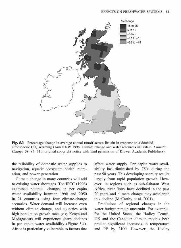
EFFECTS ON FRESHWATER SYSTEMS 81
15 to 255 to 15−5 to 5−15 to −5−25 to −15
% change
Fig. 5.3 Percentage change in average annual runoff across Britain in response to a doubledatmospheric CO2 warming (Arnell NW 1998. Climate change and water resources in Britain. ClimaticChange 39: 83–110, original copyright notice with kind permission of Kluwer Academic Publishers).
the reliability of domestic water supplies tonavigation, aquatic ecosystem health, recre-ation, and power generation.
Climate change in many countries will addto existing water shortages. The IPCC (1996)examined potential changes in per capitawater availability between 1990 and 2050in 21 countries using four climate-changescenarios. Water demand will increase evenwithout climate change, and countries withhigh population growth rates (e.g. Kenya andMadagascar) will experience sharp declinesin per capita water availability (Figure 5.4).Africa is particularly vulnerable to factors that
affect water supply. Per capita water avail-ability has diminished by 75% during thepast 50 years. This developing scarcity resultslargely from rapid population growth. How-ever, in regions such as sub-Saharan WestAfrica, river flows have declined in the past20 years and climate change may acceleratethis decline (McCarthy et al. 2001).
Predictions of regional changes in thewater budget remain uncertain. For example,for the United States, the Hadley Centre,UK and the Canadian climate models bothpredict significant increases in temperatureand PE by 2100. However, the Hadley
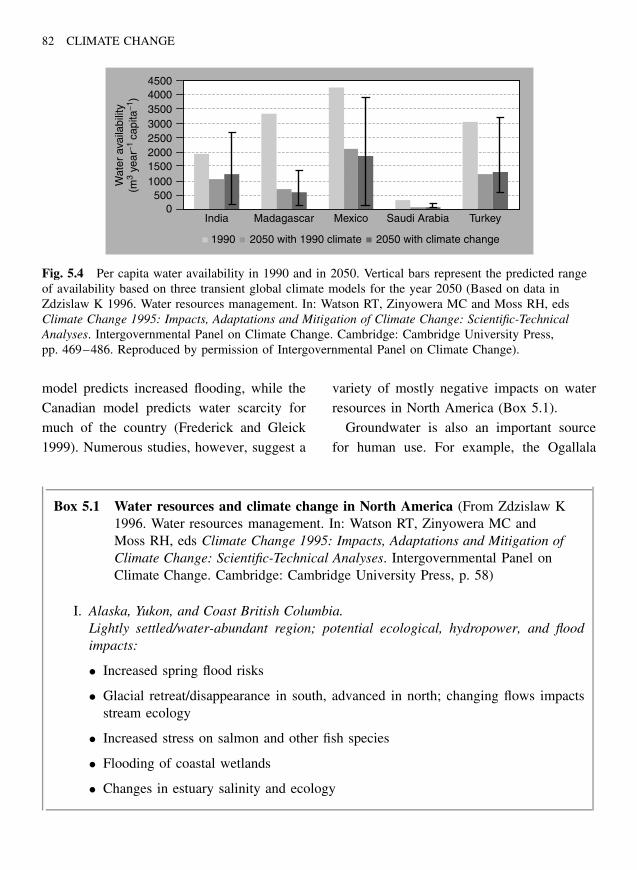
82 CLIMATE CHANGE
45004000350030002500200015001000
5000
India Madagascar
Wat
er a
vaila
bilit
y(m
3 ye
ar−1
cap
ita−1
)
Mexico Saudi Arabia Turkey
1990 2050 with 1990 climate 2050 with climate change
Fig. 5.4 Per capita water availability in 1990 and in 2050. Vertical bars represent the predicted rangeof availability based on three transient global climate models for the year 2050 (Based on data inZdzislaw K 1996. Water resources management. In: Watson RT, Zinyowera MC and Moss RH, edsClimate Change 1995: Impacts, Adaptations and Mitigation of Climate Change: Scientific-TechnicalAnalyses. Intergovernmental Panel on Climate Change. Cambridge: Cambridge University Press,pp. 469–486. Reproduced by permission of Intergovernmental Panel on Climate Change).
model predicts increased flooding, while theCanadian model predicts water scarcity formuch of the country (Frederick and Gleick1999). Numerous studies, however, suggest a
variety of mostly negative impacts on waterresources in North America (Box 5.1).
Groundwater is also an important sourcefor human use. For example, the Ogallala
Box 5.1 Water resources and climate change in North America (From Zdzislaw K1996. Water resources management. In: Watson RT, Zinyowera MC andMoss RH, eds Climate Change 1995: Impacts, Adaptations and Mitigation ofClimate Change: Scientific-Technical Analyses. Intergovernmental Panel onClimate Change. Cambridge: Cambridge University Press, p. 58)
I. Alaska, Yukon, and Coast British Columbia.Lightly settled/water-abundant region; potential ecological, hydropower, and floodimpacts:
• Increased spring flood risks
• Glacial retreat/disappearance in south, advanced in north; changing flows impactsstream ecology
• Increased stress on salmon and other fish species
• Flooding of coastal wetlands
• Changes in estuary salinity and ecology
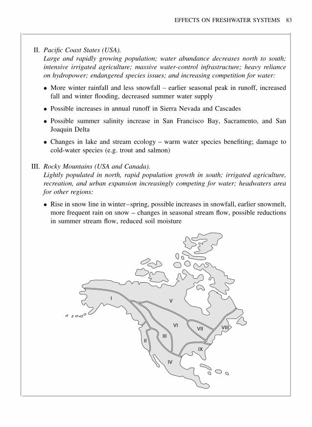
EFFECTS ON FRESHWATER SYSTEMS 83
II. Pacific Coast States (USA).Large and rapidly growing population; water abundance decreases north to south;intensive irrigated agriculture; massive water-control infrastructure; heavy relianceon hydropower; endangered species issues; and increasing competition for water:
• More winter rainfall and less snowfall – earlier seasonal peak in runoff, increasedfall and winter flooding, decreased summer water supply
• Possible increases in annual runoff in Sierra Nevada and Cascades
• Possible summer salinity increase in San Francisco Bay, Sacramento, and SanJoaquin Delta
• Changes in lake and stream ecology – warm water species benefiting; damage tocold-water species (e.g. trout and salmon)
III. Rocky Mountains (USA and Canada).Lightly populated in north, rapid population growth in south; irrigated agriculture,recreation, and urban expansion increasingly competing for water; headwaters areafor other regions:
• Rise in snow line in winter–spring, possible increases in snowfall, earlier snowmelt,more frequent rain on snow – changes in seasonal stream flow, possible reductionsin summer stream flow, reduced soil moisture
I V
VIVII
IIIII
IV
IX
VIII

84 CLIMATE CHANGE
• Stream temperature changes affecting species composition; increased isolation ofcold-water stream fish
IV. Southwest.Rapid population growth; dependence on limited groundwater and surface watersupplies; water quality concerns in border region; endangered species concerns;vulnerability to flash flooding:
• Possible changes in snowpacks and runoff
• Possible declines in groundwater recharge – reduced water supplies
• Increased water temperatures – further stress on aquatic species
• Increased frequency of intense precipitation events – increased risk of flashfloods
V. Sub-Arctic and Arctic.Sparse population (many dependent on natural systems); winter ice cover importantfeature of hydrologic cycle:
• Thinner ice cover, one- to three-month increase in ice-free season, increased extentof open water
• Increased lake-level variability, possible complete drying of some delta lakes
• Changes in aquatic ecology and species distribution as a result of warmertemperatures and longer growing season
VI. Midwest USA and Canadian Prairies.Agricultural heartland – mostly rain-fed, with some areas relying heavily on irrigation:
• Annual stream flow decreasing/increasing; possible large declines in summerstream flow
• Increasing likelihood of severe droughts
• Possible increasing aridity in semiarid zones
• Increases or decreases in irrigation demand and water availability – uncertainimpacts on farm-sector income, groundwater levels, stream flows, and water quality
VII. Great Lakes.Heavily populated and industrialized region; variations in lake levels/flows now affecthydropower, shipping, and shoreline structures:
• Possible precipitation increases coupled with reduced runoff and lake-leveldeclines
• Reduced hydropower production; reduced channel depths for shipping

EFFECTS ON FRESHWATER SYSTEMS 85
• Decreases in lake ice extent – some years without ice cover
• Changes in phytoplankton/zooplankton biomass, northward migration of fishspecies, possible extinctions of cold-water species
VIII. Northeast USA and Eastern Canada.Large, mostly urban population – generally adequate water supplies; large number ofsmall dams but limited total reservoir capacity; heavily populated floodplains:
• Decreased snow cover amount and duration
• Possible large reductions in stream flow
• Accelerated coastal erosion, saline intrusion into coastal aquifers
• Changes in magnitude, timing of ice freeze-up/breakup, with impacts onspring flooding
• Possible elimination of bog ecosystems
• Shifts in fish species distributions, migration patterns
IX. Southeast, Gulf, and Mid-Atlantic USA.Increasing population – especially in coastal areas; water quality/nonpoint sourcepollution problems; stress on aquatic ecosystems:
• Heavily populated coastal floodplains at risk to flooding from extreme precipitationevents, hurricanes
• Possible lower base flows, large peak flows, longer droughts
• Possible precipitation increase – possible increases or decreases in runoff/riverdischarge, increased flow variability
• Major expansion of northern Gulf of Mexico hypoxic zone possible – otherimpacts on coastal systems related to changes in precipitation/nonpoint sourcepollutant loading
• Changes in estuary systems and wetland extent, biotic processes, speciesdistribution.
Aquifer underlying the US Great Plains pro-vides water for about 20% of the irrigatedland in the United States. It is fully utilizedand is currently being depleted because the20 km3 of water withdrawn annually exceedsthe long-term recharge rate. Researchers atthe Pacific Northwest National Laboratoryand the US Department of Agriculture usedthree global climate models and evaluated the
effects of three different future atmosphericCO2 concentrations. Outputs from the cli-mate models, such as predicted precipitation,were linked to a hydrologic model that esti-mates parameters such as surface runoff andgroundwater recharge. Recharge of the aquiferwill be reduced under all three severities ofclimate change. For example, assuming anatmospheric CO2 concentration of 560 ppmv
86 CLIMATE CHANGE
and a global mean temperature increase of2.5 ◦C, recharge decreases by 18 to 45% overthe two major drainage basins feeding theaquifer. Climate change, forced by globalwarming, will make mining the aquifer’swater even less sustainable than it is now(Rosenberg et al. 1999).
Drought and Soil Moisture
Greenhouse warming, in some areas, will leadto higher surface air temperatures, greaterevapotranspiration, lower soil moisture, andincreasingly frequent droughts. A “droughtindex,” based on the atmospheric supply ofmoisture minus the atmospheric demand formoisture, can be used together with climatemodel outputs of precipitation and potentialevapotranspiration to evaluate the probableoccurrence of droughts. Summer droughts willbecome increasingly frequent at low latitudesand less frequent at high-latitude areas suchas Canada and Siberia (Plate 5).
Soil moisture is often the most importantfactor controlling plant growth and agri-cultural production. Globally, models pre-dict significant soil moisture changes withdecreases in some regions and increases inothers (Plate 6). Large reductions in summersoil moisture will occur in midcontinentalregions of mid to high latitudes, for example,the North American Great Plains, WesternEurope, Northern Canada, and Siberia (Man-abe et al. 1981). For example, researchers atthe University of Delaware (Mather and Fed-dema 1986) examined the effects of a dou-bling of CO2 on soil moisture at 12 selectedregions of the globe. They applied two globalclimate models to the climatic water budgeton a course grid of 8 × 10 or 4 × 5 degreeslatitude by longitude and calculated the soilmoisture index (Im):
Im = 100 [(P/PE) − 1]
where P = precipitation, PE = potential evap-otranspiration (based on field capacity of thesoil and air temperatures).
Their results for the region of North Amer-ica covering Southeastern Texas and NorthernMexico indicate that, under changed condi-tions, the months of May through Septemberwill experience no more than 5 cm of precip-itation and that peak summer evapotranspira-tion will increase by 27%. Of the 12 globalregions examined, they predict an increase inPE in all regions. Because of low tempera-tures, the warming would have little influ-ence on evapotranspiration in winter at higherlatitudes. Precipitation would increase over-all, but the additional water will be less thanthe loss due to evapotranspiration. Therefore,the annual water deficit would increase in allregions except south central Canada (NOAAmodel) and the Ukraine (GISS model). In 7 of12 areas, both models agree on a shift to drierconditions, most markedly in the upper Mid-west of the United States, the Texas–Mexicoarea, and Northeast Brazil. Overall, they con-clude that water demand will increase morethan precipitation and most regions will expe-rience an increase in annual water deficit,a decrease in annual water surplus, and adecrease in summer soil moisture storage.They predict changes in vegetation to moredrought-tolerant species in about two-thirds ofthe 12 regions studied, the exceptions beingthe Pacific Northwest, the Ukraine, and WestCentral Africa.
Finally, greenhouse warming will lead togreater heating in the eastern tropical Pacificthan in the western tropical Pacific, that is,an intensification of the El Nino pattern. Thiswill increase the intensity of future droughtsin the Australasian region (Meehl 1997).
Lake and Stream BiotaContinued warming will alter the thermal struc-ture of lakes and the impacts on lake biota are
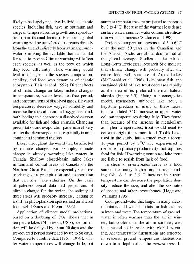
EFFECTS ON FRESHWATER SYSTEMS 87
likely to be largely negative. Individual aquaticspecies, including fish, have an optimum andrange of temperatures for growth and reproduc-tion (their thermal habitat). Heat from globalwarming will be transferred to streams directlyfromtheair and indirectly fromwarmerground-water, shrinking the available thermal habitatfor aquatic species. Climate warming will affecteach species, as well as the prey on whichthey feed, differently. Thus, warming wouldlead to changes in the species composition,stability, and food web dynamics of aquaticecosystems (Beisner et al. 1997). Direct effectsof climatic change on lakes include changesin temperature, water level, ice-free period,and concentrations of dissolved gases. Elevatedtemperatures decrease oxygen solubility andincrease the rates of microbial oxygen demand,both leading to a decrease in dissolved oxygenavailable for fish and other animals. Changingprecipitation and evaporation patterns are likelytoalter thechemistryof lakes, especially inmid-continental semiarid regions.
Lakes throughout the world will be affectedby climate change. For example, climatechange is already warming lake waters inCanada. Shallow closed-basin saline lakesin semiarid central areas of Canada on theNorthern Great Plains are especially sensitiveto changes in precipitation and evaporationthat can alter lake salinities. On the basisof paleoecological data and projections ofclimate change for the region, the salinity ofthese lakes will probably increase, leading toa shift in phytoplankton species and an alteredfood web (Evans and Prepas 1996).
Application of climate model projections,based on a doubling of CO2, shows that intemperate lakes (Minnesota, USA), ice forma-tion will be delayed by about 20 days and theice-covered period shortened by up to 58 days.Compared to baseline data (1961–1979), win-ter water temperatures will change little, but
summer temperatures are projected to increaseby 3 to 4 ◦C. Because of the warmer less densesurface water, summer water column stratifica-tion will also increase (Stefan et al. 1998).
Projected temperature increases of 3 to 6 ◦Cover the next 50 years in the Canadian andthe Alaskan Arctic are about double that ofthe global average. Studies at the AlaskaLong-Term Ecological Research Site indicatethat climate change will probably alter theentire food web structure of Arctic Lakes(McDonald et al. 1996). Like most fish, thesustained yield of lake trout decreases rapidlyas the area of its preferred thermal habitatshrinks (Figure 5.5). Using a bioenergeticsmodel, researchers subjected lake trout, akeystone predator in many of these lakes,to a simulated 3 ◦C increase in upper watercolumn temperatures during July. They foundthat, because of the increase in metabolismat higher temperatures, trout would need toconsume eight times more food. Toolik Lake,used in the study, has warmed over a recent16-year period by 3 ◦C and experienced adecrease in primary productivity that suppliesfood for fish. If warming continues, lake troutare liable to perish from lack of food.
In streams, invertebrates serve as a foodsource for many higher organisms includ-ing fish. A 2 to 3.5 ◦C increase in streamtemperature can decrease the population den-sity, reduce the size, and alter the sex ratioof insects and other invertebrates (Hogg andWilliams 1996).
Cool groundwater discharge, in many areas,maintains cold-water habitats for fish such assalmon and trout. The temperature of ground-water is often warmer than the air in win-ter, but cooler than the air in summer, andis expected to increase with global warm-ing. Air temperature fluctuations are reflectedin seasonal ground temperature fluctuationsdown to a depth called the neutral zone. In
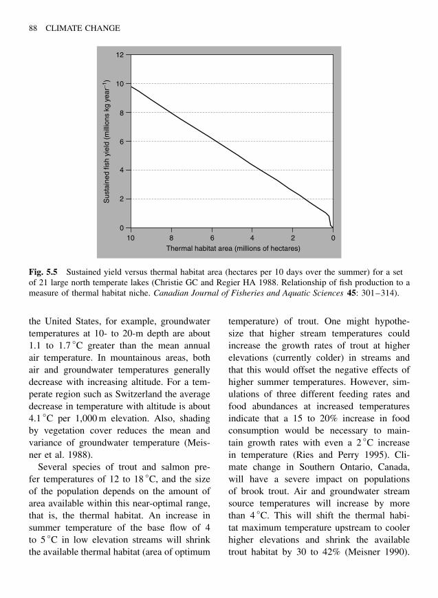
88 CLIMATE CHANGE
10
8
6
4
2
010 8 6 4
Thermal habitat area (millions of hectares)
Sus
tain
ed fi
sh y
ield
(m
illio
ns k
g ye
ar−1
)
2 0
12
Fig. 5.5 Sustained yield versus thermal habitat area (hectares per 10 days over the summer) for a setof 21 large north temperate lakes (Christie GC and Regier HA 1988. Relationship of fish production to ameasure of thermal habitat niche. Canadian Journal of Fisheries and Aquatic Sciences 45: 301–314).
the United States, for example, groundwatertemperatures at 10- to 20-m depth are about1.1 to 1.7 ◦C greater than the mean annualair temperature. In mountainous areas, bothair and groundwater temperatures generallydecrease with increasing altitude. For a tem-perate region such as Switzerland the averagedecrease in temperature with altitude is about4.1 ◦C per 1,000 m elevation. Also, shadingby vegetation cover reduces the mean andvariance of groundwater temperature (Meis-ner et al. 1988).
Several species of trout and salmon pre-fer temperatures of 12 to 18 ◦C, and the sizeof the population depends on the amount ofarea available within this near-optimal range,that is, the thermal habitat. An increase insummer temperature of the base flow of 4to 5 ◦C in low elevation streams will shrinkthe available thermal habitat (area of optimum
temperature) of trout. One might hypothe-size that higher stream temperatures couldincrease the growth rates of trout at higherelevations (currently colder) in streams andthat this would offset the negative effects ofhigher summer temperatures. However, sim-ulations of three different feeding rates andfood abundances at increased temperaturesindicate that a 15 to 20% increase in foodconsumption would be necessary to main-tain growth rates with even a 2 ◦C increasein temperature (Ries and Perry 1995). Cli-mate change in Southern Ontario, Canada,will have a severe impact on populationsof brook trout. Air and groundwater streamsource temperatures will increase by morethan 4 ◦C. This will shift the thermal habi-tat maximum temperature upstream to coolerhigher elevations and shrink the availabletrout habitat by 30 to 42% (Meisner 1990).
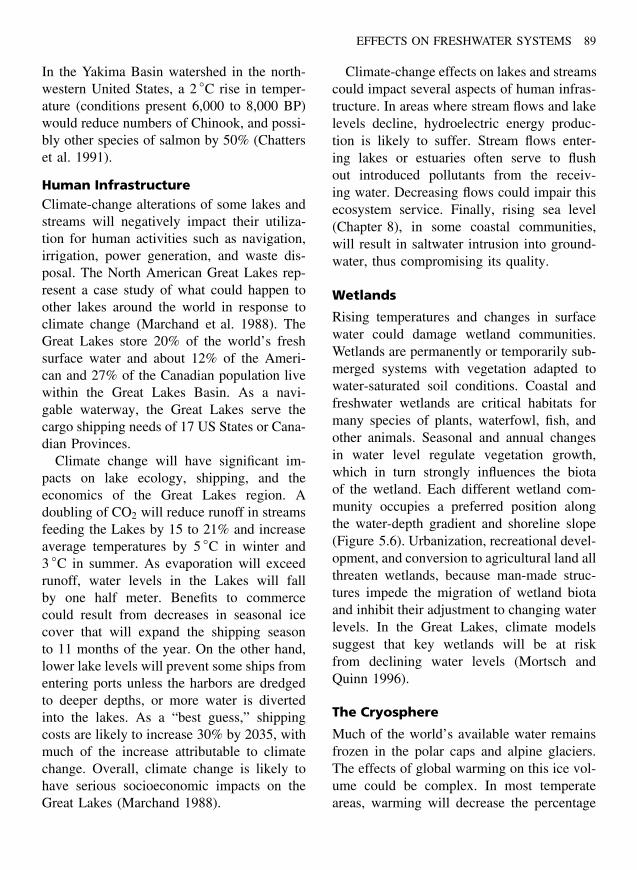
EFFECTS ON FRESHWATER SYSTEMS 89
In the Yakima Basin watershed in the north-western United States, a 2 ◦C rise in temper-ature (conditions present 6,000 to 8,000 BP)would reduce numbers of Chinook, and possi-bly other species of salmon by 50% (Chatterset al. 1991).
Human InfrastructureClimate-change alterations of some lakes andstreams will negatively impact their utiliza-tion for human activities such as navigation,irrigation, power generation, and waste dis-posal. The North American Great Lakes rep-resent a case study of what could happen toother lakes around the world in response toclimate change (Marchand et al. 1988). TheGreat Lakes store 20% of the world’s freshsurface water and about 12% of the Ameri-can and 27% of the Canadian population livewithin the Great Lakes Basin. As a navi-gable waterway, the Great Lakes serve thecargo shipping needs of 17 US States or Cana-dian Provinces.
Climate change will have significant im-pacts on lake ecology, shipping, and theeconomics of the Great Lakes region. Adoubling of CO2 will reduce runoff in streamsfeeding the Lakes by 15 to 21% and increaseaverage temperatures by 5 ◦C in winter and3 ◦C in summer. As evaporation will exceedrunoff, water levels in the Lakes will fallby one half meter. Benefits to commercecould result from decreases in seasonal icecover that will expand the shipping seasonto 11 months of the year. On the other hand,lower lake levels will prevent some ships fromentering ports unless the harbors are dredgedto deeper depths, or more water is divertedinto the lakes. As a “best guess,” shippingcosts are likely to increase 30% by 2035, withmuch of the increase attributable to climatechange. Overall, climate change is likely tohave serious socioeconomic impacts on theGreat Lakes (Marchand 1988).
Climate-change effects on lakes and streamscould impact several aspects of human infras-tructure. In areas where stream flows and lakelevels decline, hydroelectric energy produc-tion is likely to suffer. Stream flows enter-ing lakes or estuaries often serve to flushout introduced pollutants from the receiv-ing water. Decreasing flows could impair thisecosystem service. Finally, rising sea level(Chapter 8), in some coastal communities,will result in saltwater intrusion into ground-water, thus compromising its quality.
Wetlands
Rising temperatures and changes in surfacewater could damage wetland communities.Wetlands are permanently or temporarily sub-merged systems with vegetation adapted towater-saturated soil conditions. Coastal andfreshwater wetlands are critical habitats formany species of plants, waterfowl, fish, andother animals. Seasonal and annual changesin water level regulate vegetation growth,which in turn strongly influences the biotaof the wetland. Each different wetland com-munity occupies a preferred position alongthe water-depth gradient and shoreline slope(Figure 5.6). Urbanization, recreational devel-opment, and conversion to agricultural land allthreaten wetlands, because man-made struc-tures impede the migration of wetland biotaand inhibit their adjustment to changing waterlevels. In the Great Lakes, climate modelssuggest that key wetlands will be at riskfrom declining water levels (Mortsch andQuinn 1996).
The Cryosphere
Much of the world’s available water remainsfrozen in the polar caps and alpine glaciers.The effects of global warming on this ice vol-ume could be complex. In most temperateareas, warming will decrease the percentage
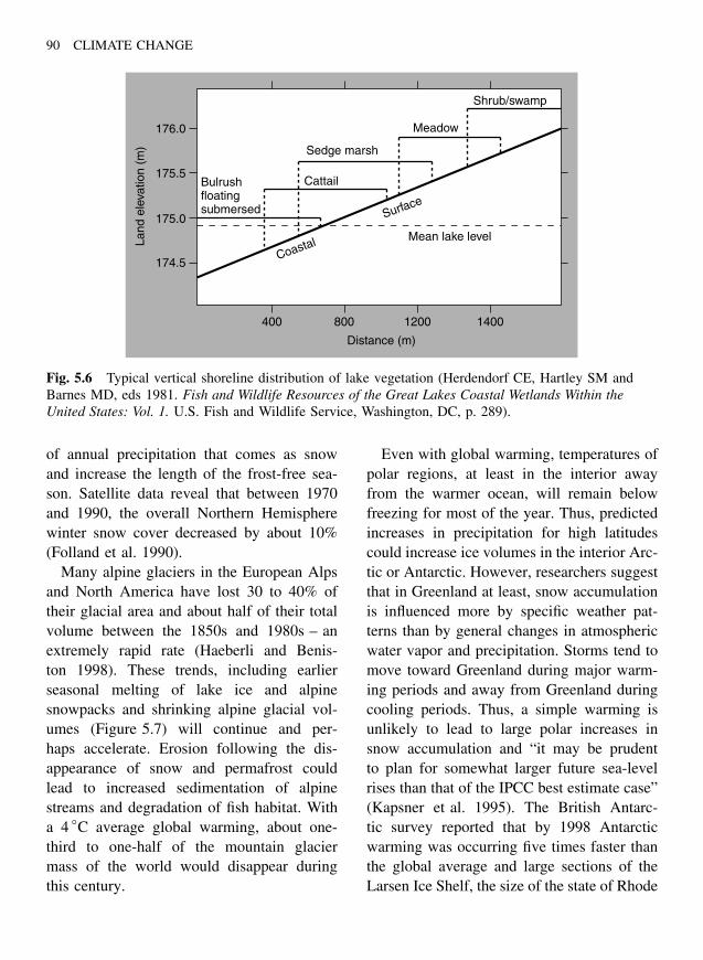
90 CLIMATE CHANGE
176.0
175.5
175.0
174.5
400 800 1200
Distance (m)
Land
ele
vatio
n (m
)
1400
Bulrushfloatingsubmersed
Sedge marsh
Cattail
Coastal
Surface
Meadow
Shrub/swamp
Mean lake level
Fig. 5.6 Typical vertical shoreline distribution of lake vegetation (Herdendorf CE, Hartley SM andBarnes MD, eds 1981. Fish and Wildlife Resources of the Great Lakes Coastal Wetlands Within theUnited States: Vol. 1. U.S. Fish and Wildlife Service, Washington, DC, p. 289).
of annual precipitation that comes as snowand increase the length of the frost-free sea-son. Satellite data reveal that between 1970and 1990, the overall Northern Hemispherewinter snow cover decreased by about 10%(Folland et al. 1990).
Many alpine glaciers in the European Alpsand North America have lost 30 to 40% oftheir glacial area and about half of their totalvolume between the 1850s and 1980s – anextremely rapid rate (Haeberli and Benis-ton 1998). These trends, including earlierseasonal melting of lake ice and alpinesnowpacks and shrinking alpine glacial vol-umes (Figure 5.7) will continue and per-haps accelerate. Erosion following the dis-appearance of snow and permafrost couldlead to increased sedimentation of alpinestreams and degradation of fish habitat. Witha 4 ◦C average global warming, about one-third to one-half of the mountain glaciermass of the world would disappear duringthis century.
Even with global warming, temperatures ofpolar regions, at least in the interior awayfrom the warmer ocean, will remain belowfreezing for most of the year. Thus, predictedincreases in precipitation for high latitudescould increase ice volumes in the interior Arc-tic or Antarctic. However, researchers suggestthat in Greenland at least, snow accumulationis influenced more by specific weather pat-terns than by general changes in atmosphericwater vapor and precipitation. Storms tend tomove toward Greenland during major warm-ing periods and away from Greenland duringcooling periods. Thus, a simple warming isunlikely to lead to large polar increases insnow accumulation and “it may be prudentto plan for somewhat larger future sea-levelrises than that of the IPCC best estimate case”(Kapsner et al. 1995). The British Antarc-tic survey reported that by 1998 Antarcticwarming was occurring five times faster thanthe global average and large sections of theLarsen Ice Shelf, the size of the state of Rhode
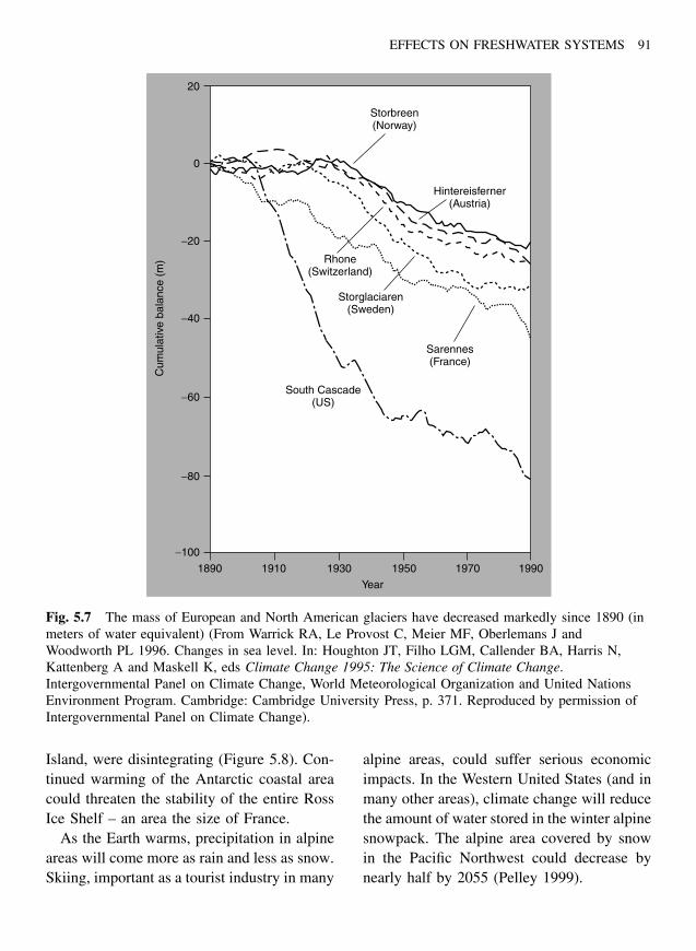
EFFECTS ON FRESHWATER SYSTEMS 91
20
−20
−40
−60
−80
−100
0
1890 1910 1930 1950
Year
1970 1990
Storbreen(Norway)
Hintereisferner(Austria)
Rhone(Switzerland)
Storglaciaren(Sweden)
Sarennes(France)
South Cascade(US)
Cum
ulat
ive
bala
nce
(m)
Fig. 5.7 The mass of European and North American glaciers have decreased markedly since 1890 (inmeters of water equivalent) (From Warrick RA, Le Provost C, Meier MF, Oberlemans J andWoodworth PL 1996. Changes in sea level. In: Houghton JT, Filho LGM, Callender BA, Harris N,Kattenberg A and Maskell K, eds Climate Change 1995: The Science of Climate Change.Intergovernmental Panel on Climate Change, World Meteorological Organization and United NationsEnvironment Program. Cambridge: Cambridge University Press, p. 371. Reproduced by permission ofIntergovernmental Panel on Climate Change).
Island, were disintegrating (Figure 5.8). Con-tinued warming of the Antarctic coastal areacould threaten the stability of the entire RossIce Shelf – an area the size of France.
As the Earth warms, precipitation in alpineareas will come more as rain and less as snow.Skiing, important as a tourist industry in many
alpine areas, could suffer serious economicimpacts. In the Western United States (and inmany other areas), climate change will reducethe amount of water stored in the winter alpinesnowpack. The alpine area covered by snowin the Pacific Northwest could decrease bynearly half by 2055 (Pelley 1999).
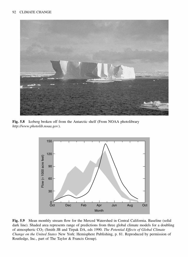
92 CLIMATE CHANGE
Fig. 5.8 Iceberg broken off from the Antarctic shelf (From NOAA photolibraryhttp://www.photolib.noaa.gov ).
150
120
90
60
30
0Oct Dec Feb Apr
Month
Flo
w (
× 10
00 a
cre
feet
)
Jun Aug Oct
Fig. 5.9 Mean monthly stream flow for the Merced Watershed in Central California. Baseline (soliddark line). Shaded area represents range of predictions from three global climate models for a doublingof atmospheric CO2 (Smith JB and Tirpak DA, eds 1990. The Potential Effects of Global ClimateChange on the United States New York: Hemisphere Publishing, p. 81. Reproduced by permission ofRoutledge, Inc., part of The Taylor & Francis Group).
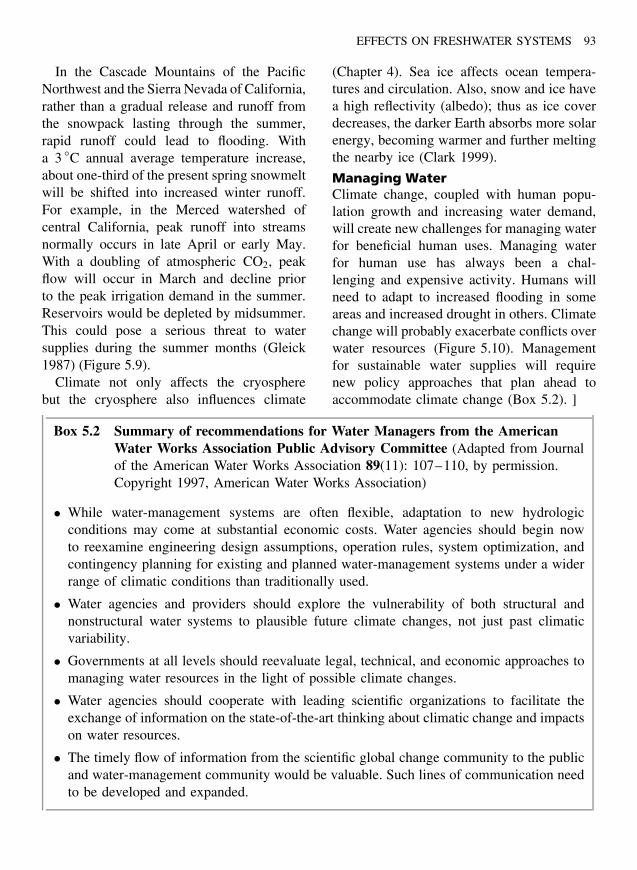
EFFECTS ON FRESHWATER SYSTEMS 93
In the Cascade Mountains of the PacificNorthwest and the Sierra Nevada of California,rather than a gradual release and runoff fromthe snowpack lasting through the summer,rapid runoff could lead to flooding. Witha 3 ◦C annual average temperature increase,about one-third of the present spring snowmeltwill be shifted into increased winter runoff.For example, in the Merced watershed ofcentral California, peak runoff into streamsnormally occurs in late April or early May.With a doubling of atmospheric CO2, peakflow will occur in March and decline priorto the peak irrigation demand in the summer.Reservoirs would be depleted by midsummer.This could pose a serious threat to watersupplies during the summer months (Gleick1987) (Figure 5.9).
Climate not only affects the cryospherebut the cryosphere also influences climate
(Chapter 4). Sea ice affects ocean tempera-tures and circulation. Also, snow and ice havea high reflectivity (albedo); thus as ice coverdecreases, the darker Earth absorbs more solarenergy, becoming warmer and further meltingthe nearby ice (Clark 1999).
Managing WaterClimate change, coupled with human popu-lation growth and increasing water demand,will create new challenges for managing waterfor beneficial human uses. Managing waterfor human use has always been a chal-lenging and expensive activity. Humans willneed to adapt to increased flooding in someareas and increased drought in others. Climatechange will probably exacerbate conflicts overwater resources (Figure 5.10). Managementfor sustainable water supplies will requirenew policy approaches that plan ahead toaccommodate climate change (Box 5.2). ]
Box 5.2 Summary of recommendations for Water Managers from the AmericanWater Works Association Public Advisory Committee (Adapted from Journalof the American Water Works Association 89(11): 107–110, by permission.Copyright 1997, American Water Works Association)
• While water-management systems are often flexible, adaptation to new hydrologicconditions may come at substantial economic costs. Water agencies should begin nowto reexamine engineering design assumptions, operation rules, system optimization, andcontingency planning for existing and planned water-management systems under a widerrange of climatic conditions than traditionally used.
• Water agencies and providers should explore the vulnerability of both structural andnonstructural water systems to plausible future climate changes, not just past climaticvariability.
• Governments at all levels should reevaluate legal, technical, and economic approaches tomanaging water resources in the light of possible climate changes.
• Water agencies should cooperate with leading scientific organizations to facilitate theexchange of information on the state-of-the-art thinking about climatic change and impactson water resources.
• The timely flow of information from the scientific global change community to the publicand water-management community would be valuable. Such lines of communication needto be developed and expanded.
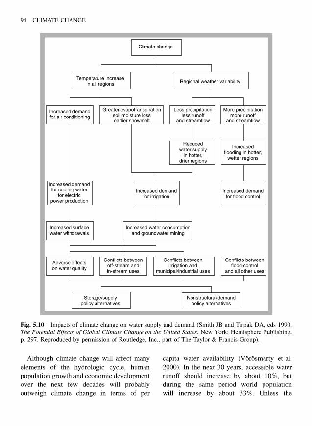
94 CLIMATE CHANGE
Climate change
Temperature increasein all regions Regional weather variability
Increased demandfor air conditioning
Greater evapotranspirationsoil moisture lossearlier snowmelt
Less precipitationless runoff
and streamflow
More precipitationmore runoff
and streamflow
Reducedwater supply
in hotter,drier regions
Increased demandfor cooling water
for electricpower production
Increased surfacewater withdrawals
Adverse effectson water quality
Storage/supplypolicy alternatives
Nonstructural/demandpolicy alternatives
Conflicts betweenoff-stream andin-stream uses
Conflicts betweenirrigation and
municipal/industrial uses
Conflicts betweenflood control
and all other uses
Increased water consumptionand groundwater mining
Increased demandfor irrigation
Increased demandfor flood control
Increasedflooding in hotter,
wetter regions
Fig. 5.10 Impacts of climate change on water supply and demand (Smith JB and Tirpak DA, eds 1990.The Potential Effects of Global Climate Change on the United States. New York: Hemisphere Publishing,p. 297. Reproduced by permission of Routledge, Inc., part of The Taylor & Francis Group).
Although climate change will affect manyelements of the hydrologic cycle, humanpopulation growth and economic developmentover the next few decades will probablyoutweigh climate change in terms of per
capita water availability (Vorosmarty et al.2000). In the next 30 years, accessible waterrunoff should increase by about 10%, butduring the same period world populationwill increase by about 33%. Unless the

EFFECTS ON FRESHWATER SYSTEMS 95
efficiency of water use can be dramaticallyincreased, per capita freshwater availabilitywill decline further. Recognizing the growingimportance of water resources and theirmanagement, UNESCO established the WorldWater Assessment Programme. The objectivesof the Programme are to develop the tools andskills needed to achieve a better understandingof basic processes, management practices, andpolicies that will help improve the supplyand quality of global freshwater resources(UNESCO 2002).
Summary
The US EPA summarized the results ofnumerous studies on the effects of climatechange on water resources of the UnitedStates (Smith and Tirpak, 1990, p. 281). Theirfindings, for the most part, still hold notonly for the United States but also for theworld. Climatic change during this centurywill probably lead to the following:
Global and regional changes in precipita-tion and evaporation:
• increasing precipitation at higher latitudesleading to increased winter/spring runoffand flooding in some areas;
• decreasing precipitation and increasingdrought frequencies at lower latitudes;
• increased summer-time evaporation anddecreasing surface flow and soil moistureat mid to high latitudes;
• decreasing lake levels in some areas;
• changes in wetland communities;
• decreasing per capita water availability,particularly in low-latitude countries withhigh population growth rates.
Higher temperatures in lakes, streams, andgroundwater sources:
• decreases in dissolved oxygen;
• changes in freshwater invertebrate and fishspecies populations.
Continued and possibly accelerated shrink-ing of snow and ice cover:
• earlier spring melting of ice cover in somelakes and polar seas;
• increased exposure of darker land massesand decreased reflectivity positively con-tributing to further warming;
• earlier runoff of spring melt water fromalpine areas.
Altogether, the changes imposed on fresh-water systems by climate change translateinto major regional impacts. In subsequentchapters we consider how these changes infreshwater, along with other changes, willinfluence natural ecosystems, agriculture, andhuman settlements and infrastructure.
References
AWWA 1997 Climate change and water resources.Committee report of the American Water WorksAssociation Public Advisory Forum. Journal ofthe American Water Works Association 89(11):107–110.
Arnell NW 1998 Climate change and water resourcesin Britain. Climatic Change 39: 83–110.
Beran M 1986 The water resource impact of futureclimate change and variability. In: Titus JG, ed.Effects of Changes in Stratospheric Ozone andGlobal Climate: Vol. 1. US. EPA, pp. 299–328.
Beisner BE, McCauley E and Wrona FJ 1997 Theinfluence of temperature and food chain lengthon plankton predator-prey dynamics. CanadianJournal of Fisheries and Aquatic Science 54:586–595.
Chatters JC, Neitzel DA, Scott MJ and Shankle SA1991 Potential impacts of global climate change onPacific Northwest Chinook salmon (Oncorhynchustshawytschia): an exploratory case study. TheNorthwest Environmental Journal 7: 71–92.
96 CLIMATE CHANGE
Christie GC and Regier HA 1988 Relationship offish production to a measure of thermal habitatniche. Canadian Journal of Fisheries and AquaticSciences 45: 301–314.
Clark PU, Alley RB and Pollard D 1999 NorthernHemisphere ice-sheet influences on global climatechange. Science 286(5442): 1104–1111.
Cubasch U and Meehl GA Projections of future cli-mate change. In: Houghton JT, Ding Y, Griggs DJ,Noguer M, van der Linden PJ, Dai X, et al., edsClimate Change 2001: The Scientific Basis Inter-governmental Panel on Climate Change, WorkingGroup 1 . Cambridge: Cambridge University Press,pp. 525–582.
Evans C and Prepas EE 1996 Potential effects of cli-mate change on ion chemistry and phytoplanktoncommunities in prairie saline lakes. Limnology andOceanography 41(5): 1063–1066.
Frederick KD and Gleick PH, Pew Center on GlobalClimate Change, 1999 Water and Global ClimateChange: Potential Impacts on US Water Resources ,p. 48.
Folland CK, Karl TR and Vinnikov KYO 1990Observed climate variations and change. In:Houghton JT, Jenkins GJ, and Ephraums JJ, edsClimate Change: the IPCC Scientific Assess-ment . Cambridge: Cambridge University Press,pp. 194–238.
Giorgi F and Hewitson B 2001 Regional cli-mate information – evaluation and projections. In:Houghton JT, Ding Y, Griggs DJ, Noguer M, vander Linden PJ, Dai X, et al. eds. Climate Change2001: The Scientific Basis. IntergovernmentalPanel on Climate Change, Working Group 1 Cam-bridge: Cambridge University Press, pp. 583–638.
Gleick PH 1987 The development and testing of awater balance model for climate impact assess-ment: modeling the Sacramento Basin. WaterResources Research 23: 1049–1061.
Haeberli W and Beniston M 1998 Climate changeand its impact on glaciers and permafrost in theAlps. Ambio 27(4): 258–265.
Herdendorf CE, Hartley SM and Barnes MD, eds1981 Fish and Wildlife Resources of the GreatLakes Coastal Wetlands Within the United States .Vol. 1. Washington, DC: U.S. Fish and WildlifeService, p. 289.
Herrington P 1996 Climate Change and the Demandfor Water London: HMSO.
Hogg ID and Williams DD 1996 Response of streaminvertebrates to a global-warming thermal regime:
an ecosystem-level manipulation. Ecology 77(2):395–407.
Kapsner WR, Alley RB, Shuman CA, Anandakrish-nan S and Grootes PM 1995 Dominant influenceof atmospheric circulation on snow accumulationin Greenland over the past 18,000 years. Nature373: 52–54.
Lockwood, JG 1999 Is potential evapotranspirationand its relationship with actual evapotranspirationsensitive to elevated atmospheric CO2 levels?Climatic Change 41: 193–212.
Manabe S, Wetherald RT and Stouffer RJ 1981 Sum-mer dryness due to an increase of atmospheric CO2
concentration. Climatic Change 3: 347–385.Marchand D, Sanderson M, Howe D and Alpaugh C
1988 Climatic change and great lakes levelsthe impact on shipping. Climatic Change 12:107–133.
Mather JR and Feddema J 1986 Hydrologic conse-quences of increases in trace gases and CO2 in theatmosphere. In: Titus JG, ed. Effects of Changesin Stratospheric Ozone and Global Climate, Vol. 3:Climate Change. Proceedings of the InternationalConference on Health and Environmental Effects ofOzone Modification and Climate Change, October1986. UNEP and US EPA, pp. 251–271.
Mauritis la Riviere JW 1989 Threats to the world’swater. Scientific American 261(3): 80–94.
McCarthy JJ, Canziani OF, Leary NA, Dokken DJand White KS, eds Climate Change 2001: Impacts,Adaptation and Vulnerability. IntergovernmentalPanel on Climate Change, Working Group II.Cambridge: Cambridge University Press, p. 45.
McDonald ME, Hershey AE and Miller MC 1996Global warming impacts on lake trout in arc-tic lakes. Limnology and Oceanography 41(5):1102–1108.
Meehl GA 1997 Pacific region climate change.Ocean and Coastal Management 37(1): 137–147.
Meisner JD 1990 Potential loss of thermal habitatfor brook trout, due to climatic warming, in twosouthern Ontario streams. Trans. Amer. FisheriesSoc. 119: 282–291.
Meisner JD, Rosenfeld JS and Regier HA 1988 Therole of groundwater in the impact of climatewarming on stream salmonids. Fisheries 13(3):2–7.
Mortsch L and Quinn F 1966 Climate change sce-narios for Great Lakes Basin ecosystem studies.Limnology and Oceanography 41: 903–911.
EFFECTS ON FRESHWATER SYSTEMS 97
Palmer T and Raisanen J 2002 Quantifying the riskof extreme seasonal precipitation events in achanging climate. Nature 415: 512–514.
Pelley J 1999 Predicted summer water shortagesattributed to climate change. Environ. Sci. Technol.33(15): 305A.
Ries RD and Perry SA 1995 Potential effects ofglobal climate warming on brook trout growth andprey consumption in central Appalachian streams,USA. Climate Research 5(3): 197–206.
Rind D, Goldberg R, Hansen J, Rosenweig C andRuedy R 1990 Potential evapotranspiration and thelikelihood of future drought. Journal of Geophys.Res. 95: 9983–10004.
Rosenberg NJ, Epstein DJ, Wang D, Vail L, Srini-vasan R and Arnold JG 1999 Possible impactsof global warming on the hydrology of theOgallala aquifer region. Climatic Change 42:677–692.
Schneider SH, Gleick PH and Mearns LO 1990Prospects for climate change. In: Waggoner PE, ed.Climate Change and U.S. Water Resources NewYork: John Wiley and Sons, pp. 41–73.
Smith JB and Tirpak DA, eds 1990 The PotentialEffects of Global Climate Change on the UnitedStates New York: Hemisphere Publishing.
Stefan HG, Fang X and Hondzo M 1998 Simulatedclimate change effects on year-round water tem-
peratures in temperate zone lakes. Climatic Change40: 547–576.
UNESCO 2002 World Water Assessment Programme.Available from: http://www.unesco.org/water/wwap/.
Vorosmarty CJ, Green P, Salisbury J and LammersRB 2000 Global water resources: vulnerabilityfrom climate change and population growth. Sci-ence 289: 284–288.
Waggoner PE 1991 U.S. water resources versus anannounced but uncertain climate change. Science251: 1002.
Warrick RA, Le Provost C, Meier MF, Oberlemans Jand Woodworth PL 1996. Changes in sea level.In: Houghton JT, Filho LGM, Callender BA, Har-ris N, Kattenberg A and Maskell K, eds ClimateChange 1995: The Science of Climate Change.Intergovernmental Panel on Climate Change, WorldMeteorological Organization and United NationsEnvironment Program. Cambridge: CambridgeUniversity Press, p. 371.
Zdzislaw K 1996 Water resources management. In:Watson RT, Zinyowera MC and Moss RH, edsClimate Change 1995: Impacts, Adaptions andMitigation of Climate Change: Scientific-TechnicalAnalyses . Intergovernmental Panel on ClimateChange. Cambridge: Cambridge University Press,pp. 469–486.

This Page Intentionally Left Blank
Chapter 6
Effects onTerrestrialEcosystems
“As I did stand my watch upon the hill,I look’d toward Birnam, and anon, methought,
The wood began to move.”
William Shakespeare, Macbeth
Introduction
Climate, primarily temperature and precipi-tation, determine the geographic distributionof major terrestrial ecosystems (biomes) fromdeserts to rain forests. Local and regionaldifferences in soil types, watershed condi-tions, and slope angle (sun exposure) influ-ence the success of different plants. However,seasonal patterns of rainfall and temperaturelargely dictate the type of plant associationsthat dominate an area – associations we calltundra, desert, grassland, rainforest, and soon. (Figure 6.1). Each plant association hasan optimum “climate space,” that is, a specificcombination of temperature and precipitationconditions in which it best thrives.
Terrestrial ecosystems are an integral partof the global carbon cycle. Grasslands andforests sequester atmospheric carbon (CO2)
through photosynthesis and store it temporarilyas organic carbon. Below ground, organiccarbon is decomposed by microorganisms andreleased back into the atmosphere. Both theseprocesses are influenced by temperature andcould be altered by global warming.
Forests and other terrestrial biomes providehabitats for a diversity of plants and animals.If the forest is damaged or removed, habitatloss can endanger the survival of the asso-ciated living organisms. Climate change candirectly affect many plants and animals byaltering the growing season or temperaturepatterns that trigger life cycle changes.
In some countries, forests occupy a majorportion of the total land area (e.g. 33% inthe United States) and serve many importantfunctions. They influence the availability andrunoff of water (see Chapter 5) and providesites for recreation and for the harvesting
Climate Change: Causes, Effects, and Solutions John T. Hardy 2003 John Wiley & Sons, Ltd ISBNs: 0-470-85018-3 (HB); 0-470-85019-1 (PB)
99
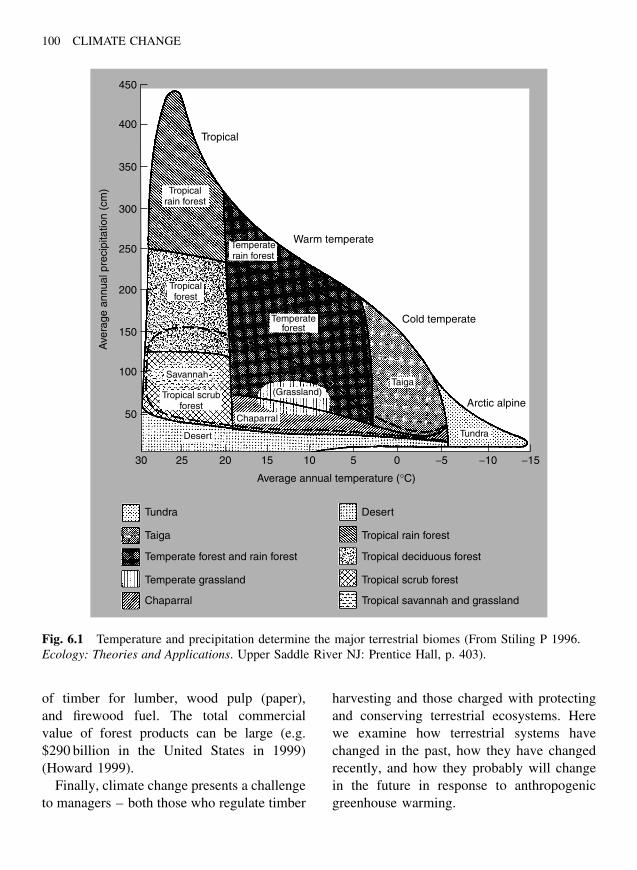
100 CLIMATE CHANGE
450
400
350
300
250
200
150
100
50
30 25 20 15 10 5
Average annual temperature (°C)
Ave
rage
ann
ual p
reci
pita
tion
(cm
)
0 −5 −10 −15
Tropicalrain forest
Temperaterain forest
Tropicalforest
Temperateforest
Savannah
Tropical scrubforest
Chaparral
Desert
(Grassland)Taiga
Tundra
Tropical
Warm temperate
Cold temperate
Arctic alpine
Desert
Tropical rain forest
Tropical deciduous forest
Tropical scrub forest
Tropical savannah and grassland
Tundra
Taiga
Temperate forest and rain forest
Temperate grassland
Chaparral
Fig. 6.1 Temperature and precipitation determine the major terrestrial biomes (From Stiling P 1996.Ecology: Theories and Applications. Upper Saddle River NJ: Prentice Hall, p. 403).
of timber for lumber, wood pulp (paper),and firewood fuel. The total commercialvalue of forest products can be large (e.g.$290 billion in the United States in 1999)(Howard 1999).
Finally, climate change presents a challengeto managers – both those who regulate timber
harvesting and those charged with protectingand conserving terrestrial ecosystems. Herewe examine how terrestrial systems havechanged in the past, how they have changedrecently, and how they probably will changein the future in response to anthropogenicgreenhouse warming.
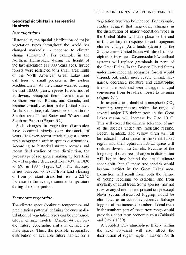
EFFECTS ON TERRESTRIAL ECOSYSTEMS 101
Geographic Shifts in TerrestrialHabitats
Past migrations
Historically, the spatial distribution of majorvegetation types throughout the world haschanged markedly in response to climatechange (Chapter 3). For example, in theNorthern Hemisphere during the height ofthe last glaciation (18,000 years ago), spruceforests were restricted to a small area southof the North American Great Lakes andoak trees to small pockets in the easternMediterranean. As the climate warmed duringthe last 18,000 years, spruce forests movednorthward, occupied their present area inNorthern Europe, Russia, and Canada, andbecame virtually extinct in the United States.At the same time, oak forests expanded in theSoutheastern United States and Western andSouthern Europe (Figure 6.2).
Such changes in vegetation distributionhave occurred slowly over thousands ofyears. However, recent trends suggest a morerapid geographic shift in species distributions.According to historical written records andrecent field studies of tree distribution, thepercentage of red spruce making up forests inNew Hampshire decreased from 40% in 1830to 6% in 1987 (Figure 6.3). The decreaseis not believed to result from land clearingor from pollutant stress but from a 2.2 ◦Cincrease in the average summer temperatureduring the same period.
Temperate vegetation
The climate space (optimum temperature andprecipitation patterns) defining the current dis-tribution of vegetation types can be measured.Global climate models (Chapter 4) can pre-dict future geographic shifts in defined cli-mate spaces. Thus, the possible geographicdistribution of available future habitat for a
vegetation type can be mapped. For example,studies suggest that large-scale changes inthe distribution of major vegetation types inthe United States will take place by the endof this century in response to anthropogenicclimate change. Arid lands (desert) in theSouthwestern United States will shrink as pre-cipitation increases. Savanna/shrub/woodlandsystems will replace grasslands in parts ofthe Great Plains. In the Eastern United Statesunder more moderate scenarios, forests wouldexpand, but, under more severe climate sce-narios, decreased moisture and catastrophicfires in the southeast would trigger a rapidconversion from broadleaf forest to savanna(Figure 6.4).
In response to a doubled atmospheric CO2
warming, temperatures within the range ofseveral major US timber trees in the GreatLakes region will increase by 7 to 10 ◦C.This will exceed the climatic tolerance of anyof the species under any moisture regime.Beech, hemlock, and yellow birch will allbe reduced in abundance in the Great Lakesregion and their optimum habitat space willshift northwest into Canada. Because of thelongevity of such trees, changes in distributionwill lag in time behind the actual climatespace shift, but all these tree species wouldbecome extinct in the Great Lakes area.Extinction will result from both the failureof young seedlings to establish and frommortality of adult trees. Some species may notsurvive anywhere in their present range exceptNova Scotia. Hardwood logging would beeliminated as an economic resource. Salvagelogging of the increased number of dead treesin the southern part of the current range wouldprovide a short-term economic gain (Zabinskiand Davis 1989).
A doubled CO2 atmosphere (likely withinthe next 50 years) will also affect thedistribution of sugar maple in Eastern North
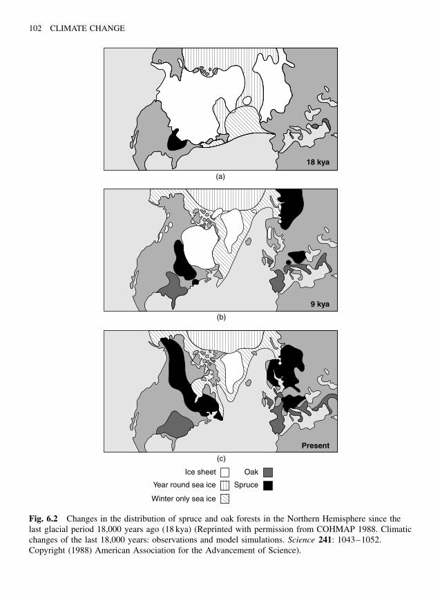
102 CLIMATE CHANGE
18 kya
9 kya
Present
Ice sheet
Year round sea ice
Oak
Spruce
Winter only sea ice
(a)
(b)
(c)
Fig. 6.2 Changes in the distribution of spruce and oak forests in the Northern Hemisphere since thelast glacial period 18,000 years ago (18 kya) (Reprinted with permission from COHMAP 1988. Climaticchanges of the last 18,000 years: observations and model simulations. Science 241: 1043–1052.Copyright (1988) American Association for the Advancement of Science).

EFFECTS ON TERRESTRIAL ECOSYSTEMS 103
45 21
20
19
18
17
40
35
30
25
20
15
10
5
01770
Picea rubens
1870
Year (AD)
Per
cent
Pic
ea r
uben
s
Mea
n su
mm
er te
mpe
ratu
re (
°C)
1970
Mean summer temperature (°C)
Fig. 6.3 Decrease in percent of red spruce (Picea rubens) in old growth stands in New England inresponse to increasing temperature since 1770 (Based on data from Hamburg SP and Coghill CV 1988.Historical decline in red spruce populations and climatic warming. Nature 331: 428–431. Copyright(1988) Macmillan Magazines Limited).
America. Increased temperature, combinedwith a decrease in soil moisture, will shiftsugar maple habitat northeast. The specieswill completely disappear from much of itscurrent range and survive only in a much-reduced area to the northeast (Figure 6.5).
In the wet coastal mountains of Californiaand Oregon, Douglas fir will shrink in thelowlands and be replaced by more drought-tolerant western pine species. In the SierraNevada mountains of California and the Cas-cade mountains of Oregon and Washington,a 2.5 to 5 ◦C warming will shift the cur-rent species composition. The postwarmingspecies composition on the west slope willmore closely match that of the currently lessdense east slope forests, reducing biomass toabout 60% of present levels (Franklin et al.1991). Current east slope forests will grad-ually shift to a drier juniper and sagebrushsystem (Figure 6.6). Overall, in the Western
United States, climate shifts will favor moredrought-tolerant species such as pine at theexpense of other species. The frequency offorest fires could increase, reducing the totalforest area.
However, considering shifting climatespaces alone may be misleading when itcomes to predicting future plant distribu-tion. Microcosm research suggests that dis-persal mechanisms and species interactionsare important and must be included for accu-rate predictions of biotic change in rela-tion to climate (Davis et al. 1998). Duringpast glacial–interglacial climatic changes, treespecies populations expanded into favorableregions at rates averaging 10 to 40 km per cen-tury. Geographic shifts in climate space result-ing from anthropogenic climate change willbe much more rapid. Thus, rates of seed dis-persal and colonization will be important lim-iting factors in forest survival in this century.
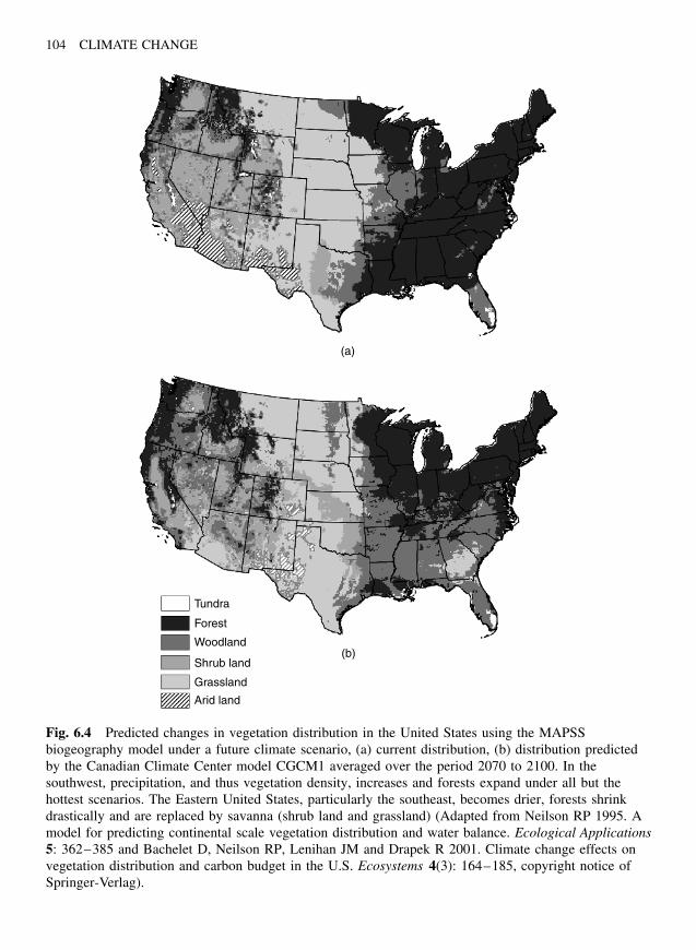
104 CLIMATE CHANGE
(a)
(b)
Tundra
Forest
Woodland
Shrub land
Grassland
Arid land
Fig. 6.4 Predicted changes in vegetation distribution in the United States using the MAPSSbiogeography model under a future climate scenario, (a) current distribution, (b) distribution predictedby the Canadian Climate Center model CGCM1 averaged over the period 2070 to 2100. In thesouthwest, precipitation, and thus vegetation density, increases and forests expand under all but thehottest scenarios. The Eastern United States, particularly the southeast, becomes drier, forests shrinkdrastically and are replaced by savanna (shrub land and grassland) (Adapted from Neilson RP 1995. Amodel for predicting continental scale vegetation distribution and water balance. Ecological Applications5: 362–385 and Bachelet D, Neilson RP, Lenihan JM and Drapek R 2001. Climate change effects onvegetation distribution and carbon budget in the U.S. Ecosystems 4(3): 164–185, copyright notice ofSpringer-Verlag).
EFFECTS ON TERRESTRIAL ECOSYSTEMS 105
0 400 km 0 400 km
Prediction based on increased temperature Prediction based on increased temperatureand moisture reduction
Present range Predicted rangeOverlap
Fig. 6.5 Predicted shift in the geographic distribution of sugar maple in North America in response toa doubling of atmospheric carbon dioxide (Adapted from Davis MB and Zabinski C 1992. Changes ingeographical range resulting from greenhouse warming: effects on biodiversity of forests. In: Peters RLand Lovejoy TE, eds Global Warming and Biological Diversity. New Haven: Yale University Press,pp. 297–308).
Boreal and alpine vegetation
Future climate changes will probably begreater at high latitudes (Chapter 4). Paleo-climatological records show past dramaticshifts in the distribution of vegetation athigh latitudes. Northern Canada and Alaskaare already experiencing rapid warming andreductions in ice cover (Chapter 3). A warmerand wetter climate at high latitudes willshift the vegetation away from cold-lovingtundra plants toward more temperate forestspecies (Starfield and Chapin 1996). Tundra,taiga, and temperate forest systems will allmigrate poleward (Monserud et al. 1993). Forexample, the distribution and area cover ofnine different vegetation types in Siberia will
be “almost completely changed” by a doubledCO2 climate (Figure 6.7).
As the climate warms, alpine plant speciesmay be forced to occupy higher mountainelevations. Studies in the European Alpssuggest that such a trend may already beunder way with the number of species ofalpine plants increasing at higher elevations(Grabherr et al. 1994). Eventually, as theirhabitat shrinks to small mountaintops, plantscould be forced to extinction.
Grassland and shrub land
Changes in precipitation and moisture willalter the composition and distribution ofgrasslands and shrub lands. Semiarid grassand shrub lands are under stress from human
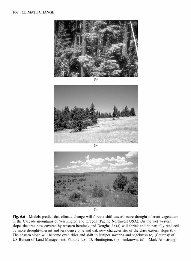
106 CLIMATE CHANGE
(a)
(b)
(c)
Fig. 6.6 Models predict that climate change will force a shift toward more drought-tolerant vegetationin the Cascade mountains of Washington and Oregon (Pacific Northwest USA). On the wet westernslope, the area now covered by western hemlock and Douglas fir (a) will shrink and be partially replacedby more drought-tolerant and less dense pine and oak now characteristic of the drier eastern slope (b).The eastern slope will become even drier and shift to Juniper savanna and sagebrush (c) (Courtesy ofUS Bureau of Land Management. Photos: (a) – D. Huntington, (b) – unknown, (c) – Mark Armstrong).
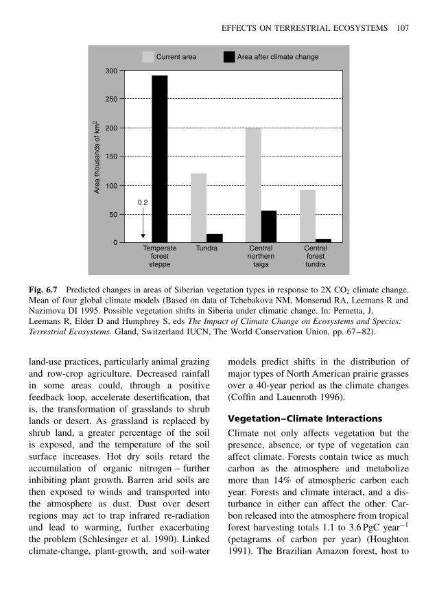
EFFECTS ON TERRESTRIAL ECOSYSTEMS 107
300
Current area Area after climate change
250
200
150
100
50
0Temperate
foreststeppe
Tundra Centralnorthern
taiga
Centralforesttundra
0.2
Are
a th
ousa
nds
of k
m2
Fig. 6.7 Predicted changes in areas of Siberian vegetation types in response to 2X CO2 climate change.Mean of four global climate models (Based on data of Tchebakova NM, Monserud RA, Leemans R andNazimova DI 1995. Possible vegetation shifts in Siberia under climatic change. In: Pernetta, J,Leemans R, Elder D and Humphrey S, eds The Impact of Climate Change on Ecosystems and Species:Terrestrial Ecosystems. Gland, Switzerland IUCN, The World Conservation Union, pp. 67–82).
land-use practices, particularly animal grazingand row-crop agriculture. Decreased rainfallin some areas could, through a positivefeedback loop, accelerate desertification, thatis, the transformation of grasslands to shrublands or desert. As grassland is replaced byshrub land, a greater percentage of the soilis exposed, and the temperature of the soilsurface increases. Hot dry soils retard theaccumulation of organic nitrogen – furtherinhibiting plant growth. Barren arid soils arethen exposed to winds and transported intothe atmosphere as dust. Dust over desertregions may act to trap infrared re-radiationand lead to warming, further exacerbatingthe problem (Schlesinger et al. 1990). Linkedclimate-change, plant-growth, and soil-water
models predict shifts in the distribution ofmajor types of North American prairie grassesover a 40-year period as the climate changes(Coffin and Lauenroth 1996).
Vegetation–Climate Interactions
Climate not only affects vegetation but thepresence, absence, or type of vegetation canaffect climate. Forests contain twice as muchcarbon as the atmosphere and metabolizemore than 14% of atmospheric carbon eachyear. Forests and climate interact, and a dis-turbance in either can affect the other. Car-bon released into the atmosphere from tropicalforest harvesting totals 1.1 to 3.6 PgC year−1
(petagrams of carbon per year) (Houghton1991). The Brazilian Amazon forest, host to
108 CLIMATE CHANGE
Box 6.1 How vegetation changes affect climate
Deforestation will probably have serious long-term irreversible effects on the climate ofthe Amazon Basin. Assuming that current trends in human habitat alteration continue, thetropical Amazon rainforest will be completely replaced by pastureland in a few decades.Researchers applied a climate model to describe the temperature, wind, and humidity of theAmazon at 18 elevations between the ground surface and 30-km altitude. The horizontalresolution was 1.8 by 2.8 km (Shulka et al. 1990). Within each grid, the vegetation wasdefined as 1 of 12 different vegetation types. They first ran the model under the presentconditions of vegetation distribution and then, with the forest converted to pasture. Comparedto the forest system, the pasture has a much greater stomatal resistance, that is, lesscapacity for transporting water from the soil to the atmosphere through plants and theirleaves. A shallower, sparser root system results in a greatly reduced soil-water storagecapacity. The surface and soil temperatures will be 1 to 3 ◦C warmer after deforestation.Less evapotranspiration leads to a reduction in atmospheric moisture, cloud formation, andprecipitation over the entire Amazon region. The overall disruption of the hydrologic cyclewill have negative impacts on plant–animal relationships. Once removed, the Amazonforest will be unable to reestablish itself. Deforestation of tropical rainforests elsewherewill probably have similar effects on regional climates.
half the world’s species, and a storehouse ofan estimated 70 PgC, is being deforested at arate of 25,000 to 50,000 km2 per year – muchof it being converted to pastureland. Thisconversion will alter the regional climate(Box 6.1).
When old-growth forests are harvested andreplaced by young forests, carbon storage asbiomass decreases substantially. Even whenstorage of carbon as lumber in wooded build-ings is included, timber harvesting results in anet positive flux of carbon to the atmosphere.In the United States, harvest of old-growthtimber in Western Washington and Oregonalone over the last 100 years has added 1.5to 1.8 PgC to the atmosphere (Harmon et al.1990). One modeling strategy uses satelliteimagery to map forest harvest activity andlink it to a carbon flux model. This approachsuggests that a single 1.2 million hectare areaof Western Oregon used for timber lands con-tributed 0.018 PgC to the atmosphere between
1972 and 1991 or about 1.13 million g C ha−1
year−1 (Cohen et al. 1996).Increasing atmospheric CO2 generally in-
creases photosynthetic rates in individualplants. However, this increased productivitydoes not necessarily benefit plants. When sev-eral species are grown together, increasedcompetition and nutrient availability dimin-ishes any benefit of enhanced atmosphericCO2. Overall, the effects of a CO2-enhancedatmosphere on communities of vegetation arecomplex and not well understood (Bazzaz andFajer 1992).
Effects of Disturbances
Greenhouse warming will increase the fre-quency of disturbance events that impact mid-latitude temperate forests (Overpeck et al.1990). Models suggest increases in “dis-turbance weather,” that is, summer/autumndrought and thunderstorms. These changingweather patterns with increases in lightning

EFFECTS ON TERRESTRIAL ECOSYSTEMS 109
4
3
2
1
0
70
60
50
40
30
20
10
01960s 1970s 1980s 1990s
Area burned Carbon emissions
Are
a bu
rned
(mill
ion
ha y
ear−1
)
Car
bon
emis
sion
s(m
illio
n to
ns y
ear−1
)
Fig. 6.8 In North American boreal forests, the average forest area that burned in 10-year periodsdoubled over 30 years. Carbon emissions into the atmosphere increased from 21 to 53 million tons peryear (Senkowsky S 2001. A burning interest in boreal forests: researchers in Alaska link fires withclimate change. Bioscience 51(11): 916–921. Copyright, American Institute of Biological Sciences).
and wind, along with decreasing soil mois-ture, will lead to increases in forest fires. Winddamage from hurricanes and flooding fromcoastal seawater rise will also have negativeimpacts in some areas.
In response to climate change, the fre-quency and intensity of forest fires will prob-ably increase in many regions of the world.In the tropics, fires in the Amazon willincrease as a result of a longer dry sea-son (Box 6.1). Also, in Borneo and Indone-sia, strong El Ninos, possibly the result ofglobal warming, have already increased theincidence and extent of forest fires. In tem-perate and boreal regions of North Amer-ica and Russia, a number of studies suggestclimate change induced increases in forestfire seasonal severity, seasonal length, andareal extent (Stocks et al. 1998). Forest fires,through a positive feedback loop, could sig-nificantly affect climate. Warmer tempera-tures lead to more fires. These fires releasegreenhouse gases and contribute to additional
warming. In fact, an increase in forest fires isalready responsible for increasing releases ofCO2 into the atmosphere (Figure 6.8). Also,in boreal regions, soils and subsurface per-mafrost represent a large carbon reservoir.Fires remove the insulating vegetation coverthat keeps the permafrost frozen. The subse-quent microbial breakdown of the soil carboncan release large quantities of CO2 into theatmosphere (Senkowsky 2001).
Loss of Biodiversity
Climate change threatens the very survival ofsome terrestrial species. Dominant forest treespecies are the backbone of the actual forestecosystem. Tree cover provides a habitat fornumerous herbaceous plants, fungi, lichens,and small and large animals. Thus, loss of thetree species will affect virtually all the speciesthat make up a complex forest ecosystem. Thesurvival of species during climatic change willlargely depend on their ability to migrate fast

110 CLIMATE CHANGE
enough to keep up with their preferred cli-mate space.
Studies using seven general circulation cli-mate models (GCMs) and two biogeographicmodels suggest that very high (compared tofossil and historical records) migration rateswill be necessary to keep pace with anthro-pogenic climate change. After the last glacia-tion, migration rates in North America wereabout 200 km or 20 km per century for spruceor beech trees, respectively. Projections sug-gest they will not be able to keep pace withan estimated 500-km migration needed dur-ing this century (Roberts 1988). Thus, climatechange will radically increase species loss andreduce biodiversity, particularly in the higherlatitudes of the Northern Hemisphere (Mal-colm and Markham 2000).
Global warming has the potential dur-ing this century to significantly alter 35%of the world’s existing terrestrial habitats(Figure 6.9). Warming will probably favorthe most mobile species and eliminate themost sedentary ones. Populations at great-est risk are those that are rare and isolated
species in fragmented habitats or those thatare bounded by water bodies, human settle-ments, or agricultural areas. In northern coun-tries, such as Russia, Sweden, and Finland, aswell as in seven Canadian Provinces, half theexisting terrestrial habitats are at risk. In Mex-ico, by 2055, the habitat area for many animalspecies will shrink significantly as a result ofclimate change. A predicted 2.4% of specieswill lose 90% of their range and be threatenedwith extinction. In the Chihuahuan desert, thehabitat of about half of all species will prob-ably disappear (Peterson et al. 2002). In theJames and Hudson Bay areas of Canada, pro-longed ice melt periods will delay the returnof polar bears to their feeding areas. This,together with potential declines in seal popu-lations, will put bears under nutritional stress(Stirling 1993). Rapid reductions in green-house gas emissions will be necessary toreduce the threat to global biodiversity.
Finally, temperature directly affects numer-ous functions of individual animals as wellas the interactions between animal popula-tions. Studies of plant and animal migrations
0−10%10−20%20−30%30−40%40−50%
50−60%60−70%70−80%80−90%90−100%
Fig. 6.9 Terrestrial biomes will probably change in response to a doubling of atmospheric CO2. Shadesindicate the percent of climate models that predict a change in the biome in that area (From Malcolm JRand Markham A 2000. Global Warming and Terrestrial Biodiversity Decline. Report of the WorldWildlife Fund, Gland, Switzerland, p. 22).
EFFECTS ON TERRESTRIAL ECOSYSTEMS 111
during past climate changes suggest that habi-tats, along with their resident organisms, willnot simply shift northward in response towarming. Rather, plant and animal commu-nities will experience complex reorganiza-tions. Invasive species with rapid reproductivecycles are likely to be favored in a changing
environment. Weed species and pests couldbecome more dominant in some areas (Mal-colm and Markham 2000). Thus, changingclimate may have many subtle and unforeseeneffects on natural periodic events that occur inthe life cycles of plants and animals (Box 6.2,Figure 6.10).
Box 6.2 Phenological changes
The natural periodic events (phenology) that occur as part of the life cycle of most organismsare closely linked to daily, seasonal, and long-term climate cycles. Temperature affects plantsin many ways, including the length of the growing season, flowering time, and coordinationwith insect pollinators. The mating and migration times of many animals are closely linkedto temperature. For example, in many reptiles, the male:female sex ratio of offspring istemperature-dependent. In the painted turtle, an increase of 2 ◦C in mean temperature maydrastically increase this ratio and a climate change of 4 ◦C would effectively eliminatethe production of male offspring and hence lead to species extinction (Janzen 1994). Likereptiles, the reproductive cycles of cold-blooded amphibians are also sensitive to climaticchange. Thus, the migration to breeding ponds and time of spawning of two species oftoad and frog in England has occurred earlier in recent years. During the period of study,from 1978 to 1994, the time for this reproductive behavior decreased 9 to 10 days per1 ◦C increase in maximum temperature (Beebee 1995). Numerous studies suggest thatphenological changes are already occurring in plants and animals in response to climatechange (adapted from Penuelas and Filella 2001):
• Mediterranean deciduous plants now leaf out 16 days earlier and fall 13 days later than50 years ago.
• In Western Canada, trees (Populus tremuloides) bloom 26 days earlier than a century ago.
• In Europe and North America, biological spring occurs a week or more earlier.
• The growing season has increased 18 days in Eurasia and 12 days in North America overthe past two decades.
• For many plants in the temperate zone, spring flowering is occurring earlier in the season.
• Insect larval development has accelerated, for example, 3 to 6 day advancement in the lifecycle of aphids in the United Kingdom, over the past 25 years. Numbers of aphid eggslaid in Spitsbergen, Norway, increase greatly when small areas are artificially warmed(Young 1994).
• Butterflies in this decade metamorphose 11 days earlier in Northeast Spain than theydid in 1952.
112 CLIMATE CHANGE
• Bird species surveyed in the United Kingdom shifted their egg laying to nine days earlierbetween 1971 and 1995.
• In New York State, frog calling occured an average 10 days earlier during 1990 to 1999than in 1900 to 1912.
• In many areas of the world, dates for migratory birds to move have changed significantly.
Such phenological changes can have a number of detrimental consequences. One of the pri-mary impacts may be a decoupling of species interactions, for example, between plants andtheir pollinators, or between birds or predators and their food supply. Phenological effectsof climate change will probably be numerous, but at the same time, often subtle and difficultto detect. However, the changes described above, as well as many others, have occurred inresponse to a warming that is only 50% of what is expected for the twenty-first century.
Implications for Forest Managementand Conservation Policy
Predicted changes raise numerous policyquestions relevant to forest management.Long-term plans for forest management willneed to take into account the likely effectsof anthropogenic climate change. Changes inforest boundaries, brought about by climatechange, will complicate land-use policies.If timber production is reduced by climatechange, should governments open up cur-rently protected parks and wilderness areas toensure timber supplies?
It is unlikely that dispersal of most treespecies will be able to keep up with theshifting climate space. Mitigation attemptsmay include artificial seed dispersal into cli-matically suitable regions. Transplantation ofspecies into new areas may aid in preserv-ing vegetation communities under the stress ofshifting climate spaces. Such attempts, how-ever, may be frustrated by the lack of suitablesoil conditions in newer areas.
Should massive reforestation be undertakennow to help sequester CO2 added to the atmo-sphere by fossil-fuel combustion? Estimatesfor the United States indicate that to keep
pace with CO2 emissions, reforestation effortswill need to be doubled or tripled at costsof hundreds of millions of dollars. It wouldtake an estimated 100 years to reforest 40%of US forest lands. Such an effort would alsorequire changes in the complex ownershippatterns of forests. Application of new tech-nologies of plant breeding, bioengineering,transplantations, fertilization, and irrigationcould aid in mitigation. But who should paythe additional costs incurred for implement-ing new policies – landowners, forest users,consumers, or all taxpayers? Tropical forestsare being harvested at a rapid pace. Anyattempt at reversing this trend and using trop-ical forestation to sequester carbon will failunless they address the economic, social, andpolitical needs of the local people (Cairns andMeganck 1994).
There is even some doubt that massivereforestation will help mitigate greenhousewarming. The albedo (reflectivity) of forestedland is usually much lower than agriculturalor other types of land cover. Thus, convert-ing high albedo land to forest may increasewarming and offset much of the benefits ofadded carbon sequestration (Betts 2000).
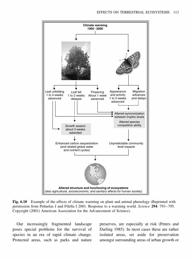
EFFECTS ON TERRESTRIAL ECOSYSTEMS 113
Climate warming1950−2000
Leaf unfolding1 to 4 weeks
advanced
Leaf fall1 to 2 weeks
delayed
FloweringAbout 1 week
advanced
Appearanceand activity
1 to 2 weeksadvanced
Migrationadvancesand delays
Growth seasonabout 3 weeks
extended
Altered syncronizationbetween trophic levels
Altered speciescompetitive ability
Enhanced carbon sequestration(and related global water
and nutrient cycles)
Unpredictable communitylevel impacts
Altered structure and functioning of ecosystems(also agricultural, socioeconomic, and sanitary effects for human society)
Fig. 6.10 Example of the effects of climate warming on plant and animal phenology (Reprinted withpermission from Penuelas J and Filella I 2001. Response to a warming world. Science 294: 793–795.Copyright (2001) American Association for the Advancement of Science).
Our increasingly fragmented landscapeposes special problems for the survival ofspecies in an era of rapid climate change.Protected areas, such as parks and nature
preserves, are especially at risk (Peters andDarling 1985). In most cases these are ratherisolated areas, set aside for preservationamongst surrounding areas of urban growth or
114 CLIMATE CHANGE
agricultural activity. As the climate changes,these nature reserves will be subject tounprecedented pressure. Only in areas withconnecting corridors will species be able tomigrate. Such a scenario suggests that newmanagement and park design strategies maybe necessary in order to preserve biodiversity.
Summary
The geographic distributions of major ter-restrial ecosystems (desert, savanna, forest,etc.) are largely governed by patterns of tem-perature and precipitation. Such systems canmigrate hundreds or thousands of kilome-ters over thousands of years in response tonatural climate change, for example, duringglacial–interglacial periods. However, suchpast migration rates are far too slow tokeep pace with the rapid geographic shifts inregional climate expected from anthropogenicgreenhouse warming. Some species may beable to migrate and keep pace with climatechange, but many may not.
There can be little doubt that climatechange during this century will signifi-cantly alter the distribution and abundanceof terrestrial species. Additional research willundoubtedly provide even more accurate sce-narios for the future. The interactions andfeedbacks between vegetation and climateneed to be more fully understood. As forestsare weakened and stressed by climate change,will their susceptibility to insect and pathogendamage, air pollution, acid rain, and forestfires result in greatly increased mortality, andwhat will be the combined effects of all suchstresses?
Changing climate appears to be responsi-ble for many documented phenological (lifecycle) changes in plants and animals over thepast 50 years or more. Future climate changecould further alter life cycle elements such as
the timing of flowering in plants, metamor-phosis in insects, or migration of animals.
Finally, if significant areas of forest arelost, what will this mean to the survivalof the numerous animal species that inhabitthe forests or streams that form part of theecosystem? Predicted changes raise manyquestions regarding the best strategy formanaging terrestrial ecosystems.
References
Bachelet D, Neilson RP, Lenihan JM and Drapek R2001 Climate change effects on vegetation distri-bution and carbon budget in the U.S. Ecosystems4(3): 164–185.
Bazzaz FA and Fajer ED 1992 Plant life in a CO2
rich world. Scientific American January: 68–74.Beebee TJC 1995 Amphibian breeding climate.
Nature 374: 219, 220.Betts RA 2000 Offset of the potential carbon sink
from boreal forestation by decreases in surfacealbedo. Nature 408: 187–190.
Cairns MA and Meganck RA 1994 Carbon seques-tration, biological diversity, sustainable develop-ment: integrated forest management. Environmen-tal Management 18(1): 13.
Coffin DP and Lauenroth WK 1996 Transientresponses of North-American grasslands to changesin climate. Climatic Change 34: 269–278.
Cohen WB, Harmon ME, Wallin DO and Fiorella M1996 Two decades of carbon flux from forestsof the Pacific Northwest. Bioscience 46(11):836–844.
COHMAP 1988 Climatic changes of the last 18,000years: observations and model simulations. Science241: 1043–1052.
Davis MB and Zabinski C 1992 Changes in geo-graphical range resulting from greenhouse warm-ing: effects on biodiversity of forests. In: Peters RLand Lovejoy TE, eds Global Warming and Biolog-ical Diversity . New Haven: Yale University Press,pp. 297–308.
Davis AJ, Jenkinson LS, Lawton JH, Shorrocks Band Wood S 1998 Making mistakes when predict-ing shifts in species range in response to globalwarming. Nature 391: 783–786.
Franklin JF, Swanson FJ, Harmon ME, Perry DA,Spies TA, Dale VH, et al. 1991 Effects of global
EFFECTS ON TERRESTRIAL ECOSYSTEMS 115
climate change on forests of northwestern NorthAmerica. The Northwest Environmental Journal 7:233–254.
Grabherr G, Gottfried M and Pauli H 1994 Climateeffects on mountain plants. Nature 369: 448.
Hamburg SP and Coghill CV 1988 Historical declinein red spruce populations and climatic warming.Nature 331: 428–431.
Harmon ME, Ferrell WK and Franklin JF 1990Effects on carbon storage of conversion of old-growth forests to young forests. Science 247:699–701.
Houghton RA 1991 Tropical deforestation and atmo-spheric carbon dioxide. Climatic Change 19:99–118.
Howard JL 1999 U.S. timber production, trade con-sumption, and price statistics 1965–1997 . GeneralTechnical Report FPL–GTR–116. Madison, WI:US Department of Agriculture, Forest Service, For-est Products Laboratory, p. 76.
Janzen FJ 1994 Climate change and temperature-dependent sex determination in reptiles. Proceed-ings of the National Academy of Sciences 91:7487–7490.
Malcolm JR and Markham A 2000 Global Warmingand Terrestrial Biodiversity Decline. Report of theWorld Wildlife Fund, Gland, Switzerland, p. 22.
Monserud RA, Tchebakova NM and Leemans R 1993Global vegetation change predicted by the modifiedBudyko model. Climatic Change 25: 59–83.
Neilson RP 1995 A model for predicting continentalscale vegetation distribution and water balance.Ecological Applications 5: 362–385.
Overpeck JT, Rind D and Goldberg R 1990 Climate-induced changes in forest disturbance and vegeta-tion. Nature 343: 51–53.
Penuelas J and Filella I 2001 Response to a warmingworld. Science 294: 793–795.
Peters RL and Darling DS 1985 The greenhouseeffect and nature reserves. Bioscience 35(11):707–717.
Peterson AT, Ortega-Huerta MA, Bartley J, Sanchez-Cordero V, Soberon J, Buddemeier RH, et al.2002 Future projections for Mexican faunas under
global climate change scenarios. Nature 416:626–629.
Roberts L 1988 Is there life after climate change?Science 242: 1010–1012.
Schlesinger WH, Reynolds JF, Cunningham GL,Huenneke LF, Jarrell WM, Virginia RA, et al.1990 Biological feedbacks in global desertification.Science 247: 1043–1048.
Senkowsky S 2001 A burning interest in borealforests: researchers in Alaska link fires withclimate change. Bioscience 51(11): 916–921.
Shulka J, Nobre C and Sellers P 1990 Amazondeforestation and climate change. Science 247:1322–1325.
Starfield A and Chapin III FS 1996 Model of tran-sient changes in arctic and boreal vegetation inresponse to climate and land use change. Ecologi-cal Applications 6(3): 842–864.
Stiling P 1996 Ecology: Theories and Applica-tions . Upper Saddle River NJ: Prentice Hall,p. 255.
Stirling I 1993 Possible impacts of climatic warmingon polar bears. Canadian Wildlife Survey 16(3):21–26.
Stocks BJ, Fosberg MA, Lynham TJ, Mearns L, Wot-ton BM, Yang Q, et al. 1998 Climate change andforest fire potential in Russian and Canadian borealforests. Climate Change 38: 1–13.
Tchebakova NM, Monserud RA, Leemans R andNazimova DI 1995 Possible vegetation shifts inSiberia under climatic change. In: Pernetta J,Leemans R, Elder D and Humphrey S, eds TheImpact of Climate Change on Ecosystems andSpecies: Terrestrial Ecosystems . Gland, Switzer-land: IUCN, The World Conservation Union,pp. 67–82.
Young S 1994 Insects that carry a global warning.New Scientist 142(1923): 32–35.
Zabinski K and Davis MB 1989 Hard Times Aheadfor Great Lakes Forests: A Climate ThresholdModel Predicts Responses to CO2-Induced ClimateChange.Contract No. CR-814607-01-0, Sponsoredby the US EPA, Research Report. Minneapolis:University of Minnesota, pp. 5-1–5-19.

This Page Intentionally Left Blank
Chapter 7
Climate Changeand Agriculture
“What we eat. . . ties us to the economic, politicaland ecological order of our whole planet.”
Frances Moore Lappe 1982
Introduction
Productive agriculture is essential to feeda growing population and sustain moderncivilization. World population will probablydouble over the next 100 years. Historically,cultivation of crops arose independently inseveral areas of the world 2,500 to 8,500 yearsago. Compared to hunter-gatherers, farm-ers could harvest more food per area ofland. Agriculture supported greater popula-tion densities than hunting and gathering,and provided the excess wealth to supportskilled craftsman, governments, and armiesof conquest (Diamond 1999). Agriculturalproductivity remains at the heart of mod-ern economies.
Climate affects agriculture, a fact wellknown to every farmer. Year-to-year vari-ations in harvest are largely due to varia-tions in temperature and precipitation thatcan make the difference between bounti-ful “bumper” crops and economic ruin. For
example, the North American Great Plains – abreadbasket of cereal crops – experienced aprolonged drought in the 1930s that turned ahuge area into a “dust bowl.” The economiceffects were devastating – farmers, unable tomeet mortgage payments, lost their farmsand many migrated elsewhere in search ofwork. Again, droughts in the Central UnitedStates in 1980 and 1988 greatly reducedthe yield of corn. Animal husbandry alsodepends on favorable climatic conditions. Forexample, the area of land needed to sustaincattle production in North America increasesvery rapidly in response to decreased rainfall(Figure 7.1).
Agriculture also affects climate. Forests,a major terrestrial sink for CO2, have beengreatly reduced by agricultural land clearing.Modern agriculture depends on fossil-fuelenergy and contributes to greenhouse gasemissions. This is clearly evident in grain-fedlivestock production, where about 20,000 calof fossil fuel (for farm machinery, etc.) are
Climate Change: Causes, Effects, and Solutions John T. Hardy 2003 John Wiley & Sons, Ltd ISBNs: 0-470-85018-3 (HB); 0-470-85019-1 (PB)
117
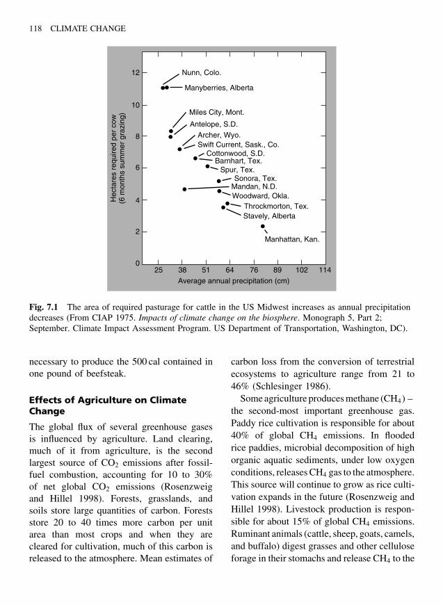
118 CLIMATE CHANGE
12
10
8
6
4
2
025 38 51 64
Average annual precipitation (cm)
Hec
tare
s re
quire
d pe
r co
w(6
mon
ths
sum
mer
gra
zing
)
76 89 102 114
Nunn, Colo.
Manyberries, Alberta
Miles City, Mont.
Antelope, S.D.
Archer, Wyo.Swift Current, Sask., Co.
Cottonwood, S.D.Barnhart, Tex.
Spur, Tex.Sonora, Tex.
Mandan, N.D.Woodward, Okla.
Throckmorton, Tex.Stavely, Alberta
Manhattan, Kan.
Fig. 7.1 The area of required pasturage for cattle in the US Midwest increases as annual precipitationdecreases (From CIAP 1975. Impacts of climate change on the biosphere. Monograph 5, Part 2;September. Climate Impact Assessment Program. US Department of Transportation, Washington, DC).
necessary to produce the 500 cal contained inone pound of beefsteak.
Effects of Agriculture on ClimateChange
The global flux of several greenhouse gasesis influenced by agriculture. Land clearing,much of it from agriculture, is the secondlargest source of CO2 emissions after fossil-fuel combustion, accounting for 10 to 30%of net global CO2 emissions (Rosenzweigand Hillel 1998). Forests, grasslands, andsoils store large quantities of carbon. Forestsstore 20 to 40 times more carbon per unitarea than most crops and when they arecleared for cultivation, much of this carbon isreleased to the atmosphere. Mean estimates of
carbon loss from the conversion of terrestrialecosystems to agriculture range from 21 to46% (Schlesinger 1986).
Some agriculture produces methane (CH4) –the second-most important greenhouse gas.Paddy rice cultivation is responsible for about40% of global CH4 emissions. In floodedrice paddies, microbial decomposition of highorganic aquatic sediments, under low oxygenconditions, releases CH4 gas to the atmosphere.This source will continue to grow as rice culti-vation expands in the future (Rosenzweig andHillel 1998). Livestock production is respon-sible for about 15% of global CH4 emissions.Ruminant animals (cattle, sheep, goats, camels,and buffalo) digest grasses and other celluloseforage in their stomachs and release CH4 to the
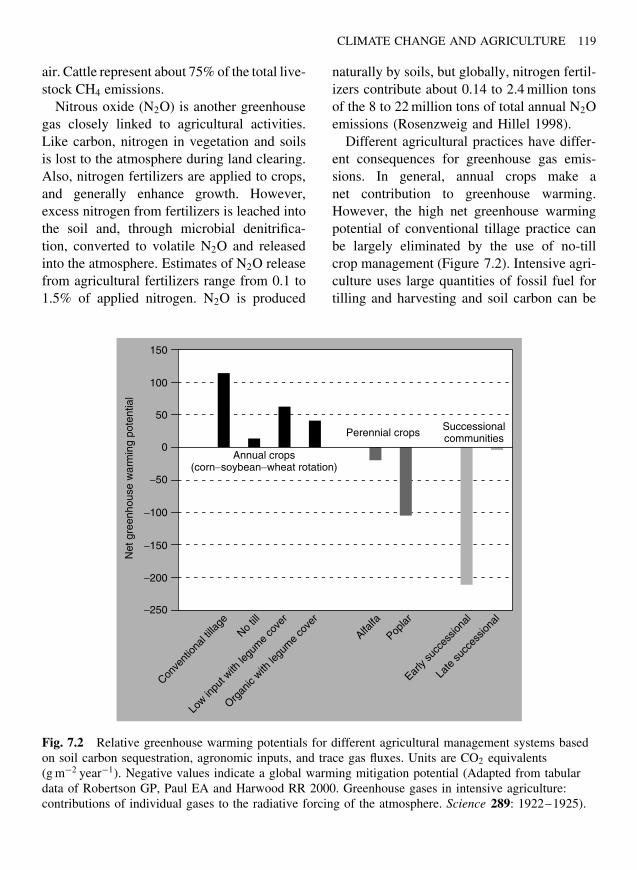
CLIMATE CHANGE AND AGRICULTURE 119
air. Cattle represent about 75% of the total live-stock CH4 emissions.
Nitrous oxide (N2O) is another greenhousegas closely linked to agricultural activities.Like carbon, nitrogen in vegetation and soilsis lost to the atmosphere during land clearing.Also, nitrogen fertilizers are applied to crops,and generally enhance growth. However,excess nitrogen from fertilizers is leached intothe soil and, through microbial denitrifica-tion, converted to volatile N2O and releasedinto the atmosphere. Estimates of N2O releasefrom agricultural fertilizers range from 0.1 to1.5% of applied nitrogen. N2O is produced
naturally by soils, but globally, nitrogen fertil-izers contribute about 0.14 to 2.4 million tonsof the 8 to 22 million tons of total annual N2Oemissions (Rosenzweig and Hillel 1998).
Different agricultural practices have differ-ent consequences for greenhouse gas emis-sions. In general, annual crops make anet contribution to greenhouse warming.However, the high net greenhouse warmingpotential of conventional tillage practice canbe largely eliminated by the use of no-tillcrop management (Figure 7.2). Intensive agri-culture uses large quantities of fossil fuel fortilling and harvesting and soil carbon can be
Conve
ntion
al till
age
No till
Low in
put w
ith le
gum
e co
ver
Organ
ic with
legu
me
cove
r
Alfalfa
Poplar
Early
succ
essio
nal
Late
succ
essio
nal
150
100
50
−50
−100
−150
−200
−250
0Annual crops
(corn−soybean−wheat rotation)
Perennial crops
Net
gre
enho
use
war
min
g po
tent
ial
Successionalcommunities
Fig. 7.2 Relative greenhouse warming potentials for different agricultural management systems basedon soil carbon sequestration, agronomic inputs, and trace gas fluxes. Units are CO2 equivalents(g m−2 year−1). Negative values indicate a global warming mitigation potential (Adapted from tabulardata of Robertson GP, Paul EA and Harwood RR 2000. Greenhouse gases in intensive agriculture:contributions of individual gases to the radiative forcing of the atmosphere. Science 289: 1922–1925).
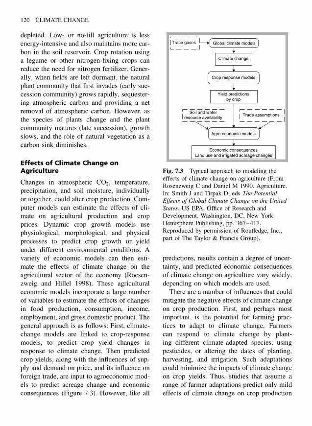
120 CLIMATE CHANGE
depleted. Low- or no-till agriculture is lessenergy-intensive and also maintains more car-bon in the soil reservoir. Crop rotation usinga legume or other nitrogen-fixing crops canreduce the need for nitrogen fertilizer. Gener-ally, when fields are left dormant, the naturalplant community that first invades (early suc-cession community) grows rapidly, sequester-ing atmospheric carbon and providing a netremoval of atmospheric carbon. However, asthe species of plants change and the plantcommunity matures (late succession), growthslows, and the role of natural vegetation as acarbon sink diminishes.
Effects of Climate Change onAgriculture
Changes in atmospheric CO2, temperature,precipitation, and soil moisture, individuallyor together, could alter crop production. Com-puter models can estimate the effects of cli-mate on agricultural production and cropprices. Dynamic crop growth models usephysiological, morphological, and physicalprocesses to predict crop growth or yieldunder different environmental conditions. Avariety of economic models can then esti-mate the effects of climate change on theagricultural sector of the economy (Roesen-zweig and Hillel 1998). These agriculturaleconomic models incorporate a large numberof variables to estimate the effects of changesin food production, consumption, income,employment, and gross domestic product. Thegeneral approach is as follows: First, climate-change models are linked to crop-responsemodels, to predict crop yield changes inresponse to climate change. Then predictedcrop yields, along with the influences of sup-ply and demand on price, and its influence onforeign trade, are input to agroeconomic mod-els to predict acreage change and economicconsequences (Figure 7.3). However, like all
Trace gases Global climate models
Climate change
Crop response models
Yield predictionsby crop
Agro-economic models
Economic consequencesLand use and irrigated acreage changes
Soil and waterresource availability
Trade assumptions
Fig. 7.3 Typical approach to modeling theeffects of climate change on agriculture (FromRosenzweig C and Daniel M 1990. Agriculture.In: Smith J and Tirpak D, eds The PotentialEffects of Global Climate Change on the UnitedStates. US EPA, Office of Research andDevelopment, Washington, DC, New York:Hemisphere Publishing, pp. 367–417.Reproduced by permission of Routledge, Inc.,part of The Taylor & Francis Group).
predictions, results contain a degree of uncer-tainty, and predicted economic consequencesof climate change on agriculture vary widely,depending on which models are used.
There are a number of influences that couldmitigate the negative effects of climate changeon crop production. First, and perhaps mostimportant, is the potential for farming prac-tices to adapt to climate change. Farmerscan respond to climate change by plant-ing different climate-adapted species, usingpesticides, or altering the dates of planting,harvesting, and irrigation. Such adaptationscould minimize the impacts of climate changeon crop yields. Thus, studies that assume arange of farmer adaptations predict only mildeffects of climate change on crop production
CLIMATE CHANGE AND AGRICULTURE 121
(Mendelsohn et al. 1994). However, farmers,even in developed countries, are not gener-ally influenced enough by long-term, subtleclimatic changes to consciously alter theirfarming operations (Smit et al. 1996). Studiesthat assume little or no farmer adaptation sug-gest very negative impacts of climate change(Rosenzweig and Parry 1994).
Second, increased atmospheric CO2 couldalso reduce the effects of climate changeon agriculture. Higher atmospheric CO2 lev-els could stimulate photosynthesis and cropproduction – a process called the CO2 fer-tilization effect. However, the magnitude ofsuch an effect is still under investigation.Greenhouse experiments on individual plantspecies demonstrate significant increases inyield. However, field experiments in whichother factors such as water and nutrient short-ages come into play often fail to show anyenhanced yields.
Third, a differential day–night warmingpattern would lessen the impacts of cli-mate change on crops. In many crops,a significant increase in daytime temper-ature maxima during the growing seasonreduces photosynthesis and increases evapo-transpiration, leading to a reduction in yield.However, recent trends and model predic-tions indicate increased cloud cover anda resulting differential warming (i.e. night-time warming increasing faster than day-time warming) (see Chapter 4). If warmingdoes occur primarily at night, rather thanduring the day, this could greatly reducethe negative impacts of climate change oncrop productivity (Dhakhwa and Campbell1998). Finally, the substitution or increaseduse of warmth-tolerant or drought-resistantcrops could mitigate the impacts of climatechange in certain areas.
However, a number of potential climateeffects could have additive or synergistic
effects, causing even more severe impactsthan most models predict. For example, onlyabout 20% of the world’s croplands areirrigated, but this land accounts for about40% of global crop production. Thus, anydecrease in water availability would result indecreased food production in regions wherewater becomes critical. Also, as crops arestressed by climate change they become morevulnerable to damaging pests and diseases.The risk of crop loss in temperate regionsmay increase as crop pests move polewardwith global warming (Porter et al. 1991).For example, aphids are a group of her-bivorous insects that can, under the rightenvironmental conditions, cause major lossesto many agricultural crops. Model ecosys-tem studies suggest that the abundance ofcertain aphids can increase dramatically inresponse to both enhanced atmospheric CO2
and increased temperature (Bezemer et al.1998). A major pest of soybeans, the potatoleafhopper Empoasca fabae, overwinters ina narrow band along the Gulf coast of theUnited States. Warmer winters would sig-nificantly expand the habitat of this pestnorthward and bring invasions earlier in thegrowing season (Figure 7.4).
Climate also affects animal husbandry.Indirect effects include climate-induced chan-ges in the availability and price of feedgrain and in pasture and forage crop yields.Extreme heat can affect the health of ani-mals. For example, heat waves can kill poul-try and decrease milk production in cows.Also, climate controls the distribution of live-stock pests and diseases (Rotter and Van deGeijn 1999).
US Agriculture
The effect of climate change on US agricul-ture is particularly important and needs to beconsidered in the global context. The United

122 CLIMATE CHANGE
States, with large areas of rich soil, favorableclimate, and modern technology, providesabout $42 billion in food exports to the world.In fact, food production and processing is theUnited States’s largest employer. Numerousstudies on the effects of climate change onagriculture have focused on the United States.
Modern large-scale agriculture is primarilymonoculture, that is, the growing of one ora few crop varieties. In the United States theeconomic value of just three crops – wheat,
corn, and soybeans – equals the value of allother crops combined (Table 7.1). With only afew species, often with specific environmentalrequirements, the practice of monoculture isparticularly vulnerable to stress, whether fromdisease, climate change, or a combinationof factors.
Studies linking climate models, crop pro-duction models, and economic models pre-dict major changes in the yield and economicvalue of US crops in response to climate
PresentFuture
Fig. 7.4 The present and future (doubled atmospheric CO2 GISS model) overwintering range of thepotato leafhopper in the Southern United States, a major pest of soybeans (From Rosenzweig C andDaniel M 1990. Agriculture. In: Smith J and Tirpak D, eds The Potential Effects of Global ClimateChange on the United States. US EPA, Office of Research and Development, Washington, DC, NewYork: Hemisphere Publishing, pp. 367–417. Reproduced by permission of Routledge, Inc., part of TheTaylor & Francis Group).
Table 7.1 Major US crops (From Myers N 1979. The Sinking Ark: A New Look atthe Problem of Disappearing Species. New York: Pergamon Press, p. 64. Reproducedwith permission of Norman Myers).
Hectares(millions
1976)
Value(millions$ 1976)
Totalvarieties
Majorvarieties
Hectarage,% of major
varieties
Corn 33,664 14,742 197 6 71Wheat 28,662 6,201 269 10 55Soybean 20,009 8,487 62 6 56Cotton 4,411 3,350 50 3 53Rice 1,012 770 14 4 65Potato 556 1,182 82 4 72Peanut 611 749 15 9 95Peas 51 22 50 2 96

CLIMATE CHANGE AND AGRICULTURE 123
change (Rosenzweig and Daniel 1990). Pro-duction of most crops will be reduced, withthe greatest reductions in sorghum (−20%),corn (−13%), and rice (−11%). Crop priceswill rise as the availability of water insome areas becomes critical and irrigation isrequired. If CO2 fertilization is considered,some areas may gain in productivity. But,nonirrigated soybean and corn yields, partic-ularly in the southeast, will drop dramatically(Figure 7.5a and 7.5b). Overall, the agricul-tural economy will shift northward in theGreat Plains and decrease in the SoutheastUnited States. In the US Midwestern GreatLakes region, an atmospheric CO2 increase to555 pmv will cause soybean yields to decreaseslightly in the south, but increase in thenorth, with an overall beneficial 40% increasein yield for the region as a whole (South-worth et al. 2002). This shift of the opti-mal production area northward in the UnitedStates will have important implications forregional economies.
Studies using three different climate mod-els and 1990 economic and agronomic condi-tions predict a range of economic impacts onUS Agriculture (Adams et al. 1995). Assum-ing a beneficial CO2 fertilization effect, overall,impacts represent only a small percentage ofthe economy. Regional differences are sig-nificant. Agroeconomies in the mountain andNorthern Plains regions gain significantly,while Eastern and Southern States experi-ence significant economic losses. Incorporat-ing technologies such as higher-yielding cropvarieties, fertilizers, herbicides, pesticides, andCO2 fertilization into models offsets most-predicted negative effects of climate change oncrop production. Conversely, most technologi-cal improvements could be offset by the addedstress of climate change. Economically, farm-ers could gain from higher crop prices, whileconsumers could lose (Figure 7.6).
A number of environmental concerns arisefrom climate impacts on US agriculture. For,example, the demand for additional agricul-tural acreage in some more northern areas,such as Minnesota and North Dakota, willput pressure on water resources and natu-ral habitats. As favorable climates move intoareas with less desirable soil, the increasedneed for fertilizers and chemicals could addto watershed or groundwater pollution. As soilmoisture decreases, the demand for irrigationwater and the energy to pump it will increasedramatically, especially in California and theGreat Plains. This will necessitate additionalinvestment in dams, irrigation projects, andpower sources. Major domestic food shortagesare unlikely, as technology is applied to offsetlosses from climate change. However, exportswill decline by about 40% as food supplies areretained for domestic consumption. ReducedUS food exports will have global economicimpacts, especially in developing countries.
Global Agriculture
Climate change will have serious impacts onworld food supplies, especially in the less-developed countries. Global warming willprobably shift growing areas by several hun-dred kilometers per degree increase in tem-perature, increasing agricultural productivityin some areas of the world, while drasticallydecreasing it in others.
In the developed countries of the TemperateZone, climate change will probably have lit-tle negative impact on agricultural production.In fact, in many temperate regions, climatewarming and an extended growing seasoncould be beneficial. In Northern Europe, cli-mate change could increase winter wheatproduction in Southern Sweden 10 to 20%over current levels by 2050. However, suchpredicted increases include many assumptions
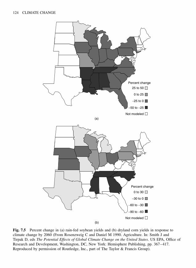
124 CLIMATE CHANGE
Percent change
25 to 50
0 to 25
−25 to 0
−50 to −25
Not modeled(a)
(b)
Percent change
0 to 30
−30 to 0
−60 to −30
−90 to −60
Not modeled
Fig. 7.5 Percent change in (a) rain-fed soybean yields and (b) dryland corn yields in response toclimate change by 2060 (From Rosenzweig C and Daniel M 1990. Agriculture. In: Smith J andTirpak D, eds The Potential Effects of Global Climate Change on the United States. US EPA, Office ofResearch and Development, Washington, DC, New York: Hemisphere Publishing, pp. 367–417.Reproduced by permission of Routledge, Inc., part of The Taylor & Francis Group).

CLIMATE CHANGE AND AGRICULTURE 125
70
60
50
40
30
20
10
−10
−20
0
Consumers US economy
Farmers
Net
cos
t in
billi
ons
of d
olla
rs
Fig. 7.6 Cost of climate change to US food-consumers, farmers, and net overall cost to economy.Negative value indicates benefit to farmers. Average predicted by two climate models. Includes changesin crop yields and supply and demand for irrigation water. Adjusted to 2001 US dollars (Adapted fromdata of Rosenzweig C and Daniel M 1990. Agriculture. In: Smith J and Tirpak D, eds The PotentialEffects of Global Climate Change on the United States. US EPA, Office of Research and Development,Washington, DC, New York: Hemisphere Publishing, pp. 367–417. Reproduced by permission ofRoutledge, Inc., part of The Taylor & Francis Group).
about the efficiency of photosynthesis, stom-atal conductance of the plants, and tempera-ture and precipitation change (Eckersten et al.2001). Australian wheat yields have increasedover the past 50 years owing to new culti-vars and changes in management practices.However, 30 to 50% of the observed increasehas been attributed to climate change, withincreases in minimum temperatures being thedominant influence (Neville 1997).
In Southern Quebec, Canada, researchersapplied the Canadian Climate Center Gen-eral Circulation Model (GCM) to examineclimatic change in response to a 2X CO2
atmosphere. They predict increases during thegrowing season in precipitation of 20 to 30%,in temperature of about 2.5 ◦C, and in grow-ing degree-days of at least 50%. The outputfrom the GCM was input to a crop model toestimate potential yield changes for a varietyof crops. Depending on the agricultural zone
and crop type, the yields increase (e.g. cornand sorghum 20%) or decrease (e.g. wheatand soybean 20 to 30%) (Singh et al. 1998).
In tropical and subtropical areas, predictedimpacts on agriculture are mostly negative.For example, in the Mediterranean region ofSouthern Europe, grain yields will probablydecrease as an increased need for irrigationplaces added demands on areas already suf-fering from acute water shortages. In poorerregions of the tropics, populations are oftenmore directly dependent on agricultural pro-duction and more affected by its failure.Certain of these regions may be particu-larly vulnerable to climate change. Low-lying coastal regions, river deltas, and islandsmay be subject to flooding by sea-level rise(Chapter 8), in which case their agriculturewould be impacted.
Water-stressed and marginal agriculturalregions (e.g. in sub-Saharan Africa, Northern

126 CLIMATE CHANGE
Mexico, the Middle East, Northeast Brazil,and Australia) may be pushed completelyout of production by climate change. InEgypt, for example, agricultural productionwill be greatly threatened by rising sealevel in the Nile Delta and by an increasedneed for irrigation from the Nile River.Model simulations suggest that wheat yieldsmay decline in the Delta by 30% and inMiddle Egypt by more than 50% – all thisin the face of a rapid growth in populationand food demand (Eid 1994). In Trinidad,combined climate change and crop modelspredict significant decreases in sugarcaneyields because of warming and increased soilmoisture stress (Singh and El Maayar 1998).
In many global regions, human-induceddeterioration of agricultural lands represents asignificant negative influence on future agri-cultural productivity. These impacts must beadded to estimates of damage from climatechange. For example, Latin America has 23%
of the world’s arable land and 30 to 40% ofthe population relies on income from agri-culture. However, 14% of the land suffersfrom moderate to extreme deterioration as aresult of overgrazing, erosion, or alkalization(a buildup of alkaline minerals in soils asa result of continued irrigation and evapora-tion). Forty seven percent of the gazing landsoils have lost their fertility. In Mexico, pre-dicted shifts toward a warmer drier climate, ina country already stressed by low and variablerainfall, could spell economic disaster. Moststudies of Latin America linking GCMs tocrop models predict major decreases in yieldfor a variety of crops (Figure 7.7).
Many areas in the Middle East and aridAsia have rapid population growth rates andare highly dependent on grazing animals andirrigated crop production. Future predictedincreases in regional water shortages, wheresmall increases in precipitation are inade-quate to counter higher evapotranspiration,
Whe
at—
Urugu
ayW
heat
—Arg
entin
aM
aize—
Argen
tina
Maiz
e—Bra
zil
Whe
at—
Brazil
Soybe
an—
Brazil
Maiz
e—M
exico
4030
2010
−10−20
−30−40
−50−60
0
Per
cent
cha
nge
in y
ield
Fig. 7.7 Percent change in crop yields in Latin America in response to climate change. Range ofestimates based on different GCMs under current conditions of technology and management (Adaptedfrom Canziani O and Diaz S 1998. Latin America. In: Watson RT, Zinyowera MC and Moss RH, edsThe Regional Impacts of Climate Change: An Assessment of Vulnerability. Special Report of IPCCWorking Group II. Cambridge: Cambridge University Press, pp. 186–230).
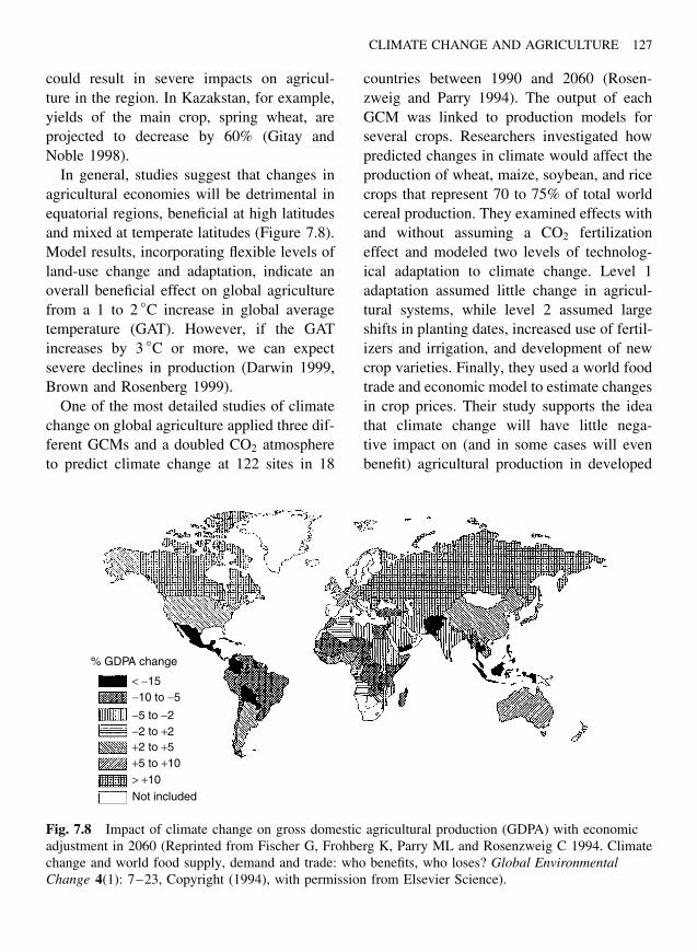
CLIMATE CHANGE AND AGRICULTURE 127
could result in severe impacts on agricul-ture in the region. In Kazakstan, for example,yields of the main crop, spring wheat, areprojected to decrease by 60% (Gitay andNoble 1998).
In general, studies suggest that changes inagricultural economies will be detrimental inequatorial regions, beneficial at high latitudesand mixed at temperate latitudes (Figure 7.8).Model results, incorporating flexible levels ofland-use change and adaptation, indicate anoverall beneficial effect on global agriculturefrom a 1 to 2 ◦C increase in global averagetemperature (GAT). However, if the GATincreases by 3 ◦C or more, we can expectsevere declines in production (Darwin 1999,Brown and Rosenberg 1999).
One of the most detailed studies of climatechange on global agriculture applied three dif-ferent GCMs and a doubled CO2 atmosphereto predict climate change at 122 sites in 18
countries between 1990 and 2060 (Rosen-zweig and Parry 1994). The output of eachGCM was linked to production models forseveral crops. Researchers investigated howpredicted changes in climate would affect theproduction of wheat, maize, soybean, and ricecrops that represent 70 to 75% of total worldcereal production. They examined effects withand without assuming a CO2 fertilizationeffect and modeled two levels of technolog-ical adaptation to climate change. Level 1adaptation assumed little change in agricul-tural systems, while level 2 assumed largeshifts in planting dates, increased use of fertil-izers and irrigation, and development of newcrop varieties. Finally, they used a world foodtrade and economic model to estimate changesin crop prices. Their study supports the ideathat climate change will have little nega-tive impact on (and in some cases will evenbenefit) agricultural production in developed
% GDPA change
< −15−10 to −5
−5 to −2−2 to +2+2 to +5+5 to +10> +10Not included
Fig. 7.8 Impact of climate change on gross domestic agricultural production (GDPA) with economicadjustment in 2060 (Reprinted from Fischer G, Frohberg K, Parry ML and Rosenzweig C 1994. Climatechange and world food supply, demand and trade: who benefits, who loses? Global EnvironmentalChange 4(1): 7–23, Copyright (1994), with permission from Elsevier Science).

128 CLIMATE CHANGE
1,600
1,400
1,200
1,000
800
600
400
200
0
Add
ition
al m
illio
n pe
ople
Withoutcarbon dioxide
fertilizationeffects
Withcarbon dioxide
fertilizationeffects
Techadaptation 1
Techadaptation 2
Fig. 7.9 Additional people at risk of hunger from climate change (Reprinted from Fischer G,Frohberg K, Parry ML and Rosenzweig C 1994. Climate change and world food supply, demand andtrade: who benefits, who loses? Global Environmental Change 4(1): 7–23, Copyright (1994), withpermission from Elsevier Science).
countries. However, in the poorer nations,the lack of technological adaptation and otherfactors will lead to a substantial decline inagricultural production (Plate 2). Because ofchanges in world food supply and demand,cereal prices will increase and the number ofpeople at risk of hunger will increase by 10sto 100s of millions (Figure 7.9).
Other case studies for different regionsof the world suggest the following (Parryet al. 1988):
• a significant increase in rice productionin Japan;
• increased droughts and crop stress in Aus-tralia, Brazil, India, and parts of Africaresulting from an intensified El Nino;
• dramatic losses in farm production inthe central plains of the United Statesand Canada as it returns to “dust bowl”conditions similar to the 1930s;
• increased production in temperate countriessuch as Finland and the Russian Federationif technological improvements can takeadvantage of warmer conditions.
Summary
Large increases in agricultural production dur-ing this century will be necessary to feed theworld’s growing human population. Crop pro-duction is very sensitive to climate conditions.Thus, increased production in many areas willbe even more difficult in the face of global cli-mate change. In the United States, food short-ages are unlikely, but investments required forirrigation and other technologies will increasefood costs and lead to decreased exports.Globally, developed countries will face thesame challenges as the United States, andcrop prices are likely to increase. The less-developed countries will be unable to applyexpensive technologies to maintain agricul-tural production and some will experiencefood shortages and increased hunger.
Many agro-climatologists cited here arepessimistic about the effects of climate changeon world agriculture. However, some sci-entists remain confident that humans canand will adapt agricultural practices so thatclimate-change impacts will be minimal oreven beneficial. Examples exist for several
CLIMATE CHANGE AND AGRICULTURE 129
grain crops. The belt for hard red winterwheat has expanded northwestward from Cen-tral United States by hundreds of kilometersduring the last part of the twentieth cen-tury through the use of different cultivarsand agronomic practices. In the case of ricebreeding, 40 to 50 selection cycles could becompleted before atmospheric CO2 reaches600 ppm (Seshu et al. 1989).
Major findings concerning the effects ofclimate change on agriculture can be summa-rized as follows:
• For a doubling of atmospheric CO2, overallglobal agricultural production seems sus-tainable. However, responses differ greatlybetween regions. Low-latitude, low-incomeareas will experience the greatest impacts.
• Sub-Saharan Africa – This arid to semi-arid region where 60% of the populationdepends directly on farming appears mostvulnerable to climate change.
• South and Southeast Asia – More than 30%of the GDP comes from agriculture andthese regions may be vulnerable.
• Pacific Island Nations – Sea-level rise andassociated saltwater intrusion could nega-tively impact agriculture.
• Technological adaptation – Increased irri-gation (where water is available), adop-tion of alternate crop varieties, and so onwill minimize impacts for those countriesthat can afford it. However, climate changecould seriously impact agriculture in devel-oping countries.
• Government agricultural policies – Manypresent policies discourage adaptation andtechnological innovation and may impedeadaptation to climate change.
References
Adams RM, Fleming RA, Chang C-C and McCarl B1995 A reassessment of the economic effects ofglobal climate change on U.S. agriculture. ClimaticChange 30: 147–167.
Bezemer TM, Hefin T and Knight KJ 1998 Long-term effects of elevated CO2 and temperatureon populations of the peach potato aphid Myzuspersicae and its parasitoid Apphidius matricariae.Oecologia 116: 128–135.
Brown RA and Rosenberg NJ 1999 Climate changeimpacts on the potential productivity of cornand winter wheat in their primary United Statesgrowing regions. Climatic Change 41: 73–107.
CIAP 1975 Impacts of Climate Change on theBiosphere. Monograph 5, Part 2; September. USDepartment of Transportation, Washington, DC.
Canziani O and Diaz S 1998 Latin America. In:Watson RT, Zinyowera MC and Moss RH, edsThe Regional Impacts of Climate Change: AnAssessment of Vulnerability . Special Report ofIPCC Working Group II. Cambridge: CambridgeUniversity Press, pp. 186–230.
Darwin R 1999 A farmer’s view of the Ricardianapproach to measuring agricultural effects ofclimatic change. Climatic Change 43: 371–411.
Dhakhwa GB and Campbell CL 1998 Potentialeffects of differential day-night warming in globalclimatic change on crop production. ClimaticChange 40: 647–667.
Diamond J 1999 Guns, Germs and Steel: The Fates ofHuman Societies . New York: W.W. Norton & Co.
Eckersten H, Blomback K, Katterer T and Nyman P2001 Modelling C, N, water and heat dynamicsin winter wheat under climate change in SouthernSweden. Agriculture Ecosystems and Environment86(3): 221–236.
Eid HM 1994 Impact of climate change on sim-ulated wheat and maize yields in Egypt. In:Rosenzweig C and Iglesias A, eds Implicationsof Climate Change for International Agriculture:Crop Modeling Study . Washington, DC: US EPA,pp. 1–14.
Fischer G, Frohberg K, Parry ML and Rosenzweig C1994 Climate change and world food supply,demand and trade: who benefits, who loses? GlobalEnvironmental Change 4(1): 7–23.
Gitay H and Noble IR 1998 Middle East andArid Asia. In: Watson RT, Zinyowera MC andMoss RH eds, The Regional Impacts of Climate
130 CLIMATE CHANGE
Change: An Assessment of Vulnerability . SpecialReport of IPCC Working Group II. Cambridge:Cambridge University Press, pp. 231–252.
Lappe FM 1982 Diet for a Small Planet . New York:Ballantine Books, p. 8.
Mendelsohn R, Nordhaus RW and Shaw D 1994The impact of global warming on agriculture:a Ricardian analysis. American Economic Review84(4): 753–771.
Myers N 1979 The Sinking Ark: A New Look atthe Problem of Disappearing Species . New York:Pergamon Press, p. 64.
Neville N 1997 Increased Australian wheat yield dueto recent climate trends. Nature 387: 484, 485.
Parry ML, Carter TR and Konijn N, eds 1988 TheImpact of Climatic Variations on Agriculture.Vol. 1: Assessments in Cool, Temperate and ColdRegions; Vol. 2: Assessments in Semi-Arid Regions .Boston: Kluwer Academic Publishers.
Porter JH, Parry ML and Carter TR 1991 The poten-tial effects of climate change on agriculturalinsect pests. Agricultural/Forest Meteorology 57:221–240.
Robertson GP, Paul EA and Harwood RR 2000Greenhouse gases in intensive agriculture: contri-butions of individual gases to the radiative forcingof the atmosphere. Science 289: 1922–1925.
Rosenzweig C, Daniel M and US EPA, Office ofResearch and Development 1990 Agriculture.In: Smith J and Tirpak D, eds The PotentialEffects of Global Climate Change on the UnitedStates . Washington, DC: Hemisphere Publishing,pp. 367–417.
Rosenzweig CR and Hillel D 1998 Climate Changeand the Global Harvest: Potential Impacts of theGreenhouse Effect on Agriculture. Oxford: OxfordUniversity Press.
Rosenzweig C and Parry M 1994 Potential impact ofclimate change on world food supply. Nature 367:133–138.
Rotter R and Van de Geijn SC 1999 Climate changeeffects on plant growth, crop yield and livestock.Climatic Change 43: 651–681.
Schlesinger WH 1986 Changes in soil carbon storageand associated properties with disturbance andrecovery. In: Trabalka JR and Reichle DE, eds TheChanging Carbon Cycle: A Global Analysis . NewYork: Springer-Verlag, pp. 194–220.
Seshu DV, Woodhead T, Garrity DP and Olde-man LR 1989 Effect of weather and climate onproduction and vulnerability of rice. Climate andFood Security. International Symposium on Cli-mate Variability and Food Security in Develop-ing Countries , 5–9 February 1987, New Delhi,India, Manila: International Rice Research Insti-tute, pp. 93–113.
Singh B and El Maayar M 1998 Potential impacts ofgreenhouse gas climate change scenarios on sugarcane yields in Trinidad. Tropical Agriculture 75(3):348–354.
Singh B, El Maayar M, Andre P, Bryant CR andThouez J-P 1998 Impacts of a GHG-induced cli-mate change on crop yields: effects of accelerationin maturation, moisture stress and optimal temper-ature. Climatic Change 38: 51–86.
Smit B, McNabb D and Smithers J 1996 Agriculturaladaptation to climatic variation. Climatic Change33: 7–29.
Southworth J, Pfeifer RA, Habeck M, Randolph JC,Doering OC, Johnston JJ, et al. 2002 Changes insoybean yields in the midwestern United Statesas a result of future changes in climate, climatevariability, and CO2 fertilization. Climatic Change53: 447–475.

Chapter 8
Climate Changeand the MarineEnvironment
“We have been sustained by the ocean for two millennia. . . this harmony may beinterrupted by the action of nations very distant from our shores. I hope that thepeoples of the Pacific [Islands] can help convince the industrialized nations to
discontinue their profligate contamination of the atmosphere.”
Amata Kabua, President of the Marshall Islands, 1989
Introduction
Humans depend on the sea. Climate changecould affect sea-level ocean–atmosphereinteractions, ocean heat transport, biogeo-chemical cycles, and marine ecosystemsincluding fisheries. Two-thirds of the Earth’ssurface is covered by ocean. As it warms,the ocean’s volume expands. This expansion,together with additional water from meltingglaciers, will raise the sea level. Higher sealevel will affect shallow water marine com-munities and greatly impact human coastalpopulations.
Physical interactions between the atmo-sphere and hydrosphere (ocean), which playa key role in determining climate, will prob-ably be altered themselves by climate change(Bigg 1996). Increasing water temperatureincreases the movement of water vapor fromthe ocean to the atmosphere (evaporation) and
decreases the solubility of atmospheric green-house gases (Chapter 1). Changes in oceantemperature and/or salinity will alter density-driven ocean currents and heat transport.Marine biogeochemical processes in the oceansuch as photosynthesis, organosulfide produc-tion, and calcium carbonate formation areinfluenced by climate. Changes in these pro-cesses, through complicated feedbacks, willsignificantly add to climate-change impacts.
Finally, global climate change will alterthe available habitat and population distribu-tion of marine plankton, invertebrates, fish,and marine mammals. Warmer temperaturesmay increase the incidence of toxic algalblooms and marine diseases. Here we exam-ine the effects of greenhouse warming on theworld’s oceans and describe how marine biotaand human communities will be affected bychanging ocean conditions.
Climate Change: Causes, Effects, and Solutions John T. Hardy 2003 John Wiley & Sons, Ltd ISBNs: 0-470-85018-3 (HB); 0-470-85019-1 (PB)
131
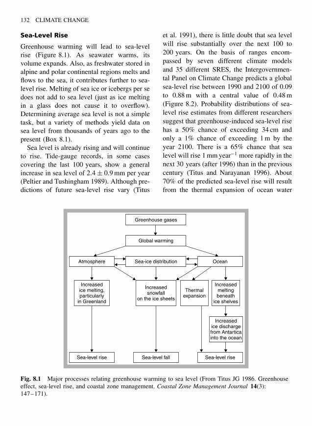
132 CLIMATE CHANGE
Sea-Level Rise
Greenhouse warming will lead to sea-levelrise (Figure 8.1). As seawater warms, itsvolume expands. Also, as freshwater stored inalpine and polar continental regions melts andflows to the sea, it contributes further to sea-level rise. Melting of sea ice or icebergs per sedoes not add to sea level (just as ice meltingin a glass does not cause it to overflow).Determining average sea level is not a simpletask, but a variety of methods yield data onsea level from thousands of years ago to thepresent (Box 8.1).
Sea level is already rising and will continueto rise. Tide-gauge records, in some casescovering the last 100 years, show a generalincrease in sea level of 2.4 ± 0.9 mm per year(Peltier and Tushingham 1989). Although pre-dictions of future sea-level rise vary (Titus
et al. 1991), there is little doubt that sea levelwill rise substantially over the next 100 to200 years. On the basis of ranges encom-passed by seven different climate modelsand 35 different SRES, the Intergovernmen-tal Panel on Climate Change predicts a globalsea-level rise between 1990 and 2100 of 0.09to 0.88 m with a central value of 0.48 m(Figure 8.2). Probability distributions of sea-level rise estimates from different researcherssuggest that greenhouse-induced sea-level risehas a 50% chance of exceeding 34 cm andonly a 1% chance of exceeding 1 m by theyear 2100. There is a 65% chance that sealevel will rise 1 mm year−1 more rapidly in thenext 30 years (after 1996) than in the previouscentury (Titus and Narayanan 1996). About70% of the predicted sea-level rise will resultfrom the thermal expansion of ocean water
Atmosphere
Sea-level rise
Greenhouse gases
Global warming
OceanSea-ice distribution
Increasedsnowfall
on the ice sheets
Increasedice melting,particularly
in Greenland
Thermalexpansion
Increasedmeltingbeneath
ice shelves
Increasedice dischargefrom Antarticainto the ocean
Sea-level fall Sea-level rise
Fig. 8.1 Major processes relating greenhouse warming to sea level (From Titus JG 1986. Greenhouseeffect, sea-level rise, and coastal zone management. Coastal Zone Management Journal 14(3):147–171).
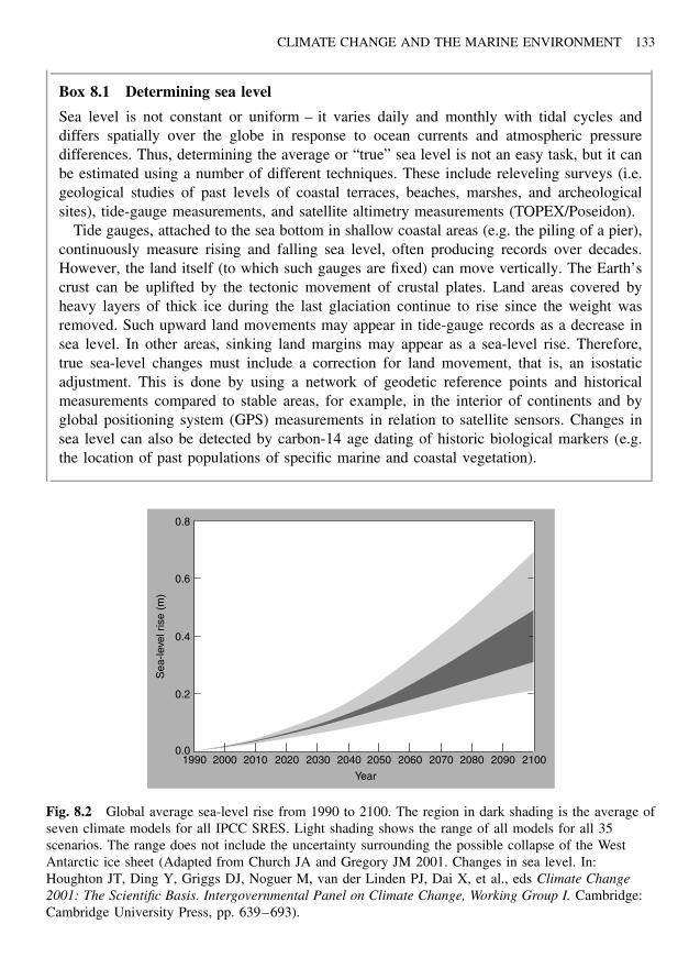
CLIMATE CHANGE AND THE MARINE ENVIRONMENT 133
Box 8.1 Determining sea level
Sea level is not constant or uniform – it varies daily and monthly with tidal cycles anddiffers spatially over the globe in response to ocean currents and atmospheric pressuredifferences. Thus, determining the average or “true” sea level is not an easy task, but it canbe estimated using a number of different techniques. These include releveling surveys (i.e.geological studies of past levels of coastal terraces, beaches, marshes, and archeologicalsites), tide-gauge measurements, and satellite altimetry measurements (TOPEX/Poseidon).
Tide gauges, attached to the sea bottom in shallow coastal areas (e.g. the piling of a pier),continuously measure rising and falling sea level, often producing records over decades.However, the land itself (to which such gauges are fixed) can move vertically. The Earth’scrust can be uplifted by the tectonic movement of crustal plates. Land areas covered byheavy layers of thick ice during the last glaciation continue to rise since the weight wasremoved. Such upward land movements may appear in tide-gauge records as a decrease insea level. In other areas, sinking land margins may appear as a sea-level rise. Therefore,true sea-level changes must include a correction for land movement, that is, an isostaticadjustment. This is done by using a network of geodetic reference points and historicalmeasurements compared to stable areas, for example, in the interior of continents and byglobal positioning system (GPS) measurements in relation to satellite sensors. Changes insea level can also be detected by carbon-14 age dating of historic biological markers (e.g.the location of past populations of specific marine and coastal vegetation).
0.8
0.6
0.4
0.2
0.01990 2000 2010 2020 2030 2040 2050
Year
Sea
-leve
l ris
e (m
)
2060 2070 2080 2090 2100
Fig. 8.2 Global average sea-level rise from 1990 to 2100. The region in dark shading is the average ofseven climate models for all IPCC SRES. Light shading shows the range of all models for all 35scenarios. The range does not include the uncertainty surrounding the possible collapse of the WestAntarctic ice sheet (Adapted from Church JA and Gregory JM 2001. Changes in sea level. In:Houghton JT, Ding Y, Griggs DJ, Noguer M, van der Linden PJ, Dai X, et al., eds Climate Change2001: The Scientific Basis. Intergovernmental Panel on Climate Change, Working Group I. Cambridge:Cambridge University Press, pp. 639–693).
134 CLIMATE CHANGE
as it warms and 30% from melting glaciersand ice caps that add freshwater to the sea.Sea-level rise will lag the global tempera-ture increase; thus sea level could continue torise for several centuries beyond 2100 to sev-eral meters above its current level. However,predictions of sea-level rise contain severaluncertainties. If the West Antarctic ice sheetmelts and collapses (a less likely, but possi-ble, scenario), sea level could increase by 6 m.Also, any changes in atmospheric circulationin the North Atlantic could alter precipitationand snow and ice accumulation in Greenland(Bromwich 1995).
Sea-level rise will have a number of impor-tant impacts on ecosystems and humans. Abouthalf the world’s population lives within 200 kmof the ocean, and many millions live in coastalareas that are less than 5 m above sea level. Sea-level rise impacts include increased beach ero-sion, saltwater intrusion into groundwater, andflooding of coastal habitats. Generally, beachloss from erosion will far exceed that expectedfrom direct inundation. The area eroded willdepend upon the average slope of the beach outto a water depth where waves cease to impactthe bottom (generally about 10 m deep) (Brunn1962). This means that in many areas a 1-cmrise in sea level would result in a shorelineretreat of 1 m, that is, sea-level rise to beachloss ratio of 1 : 100. In areas of stronger waveaction, the shore retreat would be even greater,and in areas of low beach slope, for example,parts of Florida, it could mean a sea-level rise tobeach retreat ratio of 1 : 1000. In such an area, a1-m rise in sea level would mean a 1-km retreatof the shore. For a property owner with 2 km ofbeachfront, this would mean a loss in land areaof 50%.
In many areas, beaches represent a valuableeconomic resource based on tourism. The pro-tection, stabilization, and replenishment of
these beaches will require massive invest-ments of capital to retain their economicvalue. Financial institutions are already we-ighing the risk of investing in and insuringlow-lying coastal properties (Chapter 9).
Many coastal and island communities drawtheir freshwater from groundwater wells.Because it is less dense than saltwater,fresh groundwater generally collects beneathcoastal areas or islands as a “freshwaterlens” floating on top of intruding subsurfaceseawater. As sea level rises, such freshwaterlenses will be squeezed into smaller volumes,that is, saltwater will intrude into the freshgroundwater.
Certain regions are particularly vulnerableto the effects of sea-level rise. For islandnations of the Pacific, the Indian Ocean, andthe Caribbean, erosion, flooding, and saltwaterintrusion into water supplies all threaten thesocial and economic viability of island states(Roy and Connell 1991). For example, mostof the land area of the atoll island states ofKiribati, Maldives, Marshall Islands, Tokelau,and Tuvalu, with a combined population ofgreater than 300,000, is less than 3 m abovesea level. These islands could lose muchor all of their land area to the sea. Onestudy recommends that plans be drawn upfor the relocation of major Pacific islandsettlements (Nunn 1988). Island people maybecome the first environmental refugees of thegreenhouse era.
Other areas sensitive to sea-level rise arelow-lying river deltas, for example, the Mis-sissippi, Nile, Ganges, Orinoco, and numer-ous others. A 1-m sea-level rise would dra-matically change the physical character ofthe San Francisco Bay and delta. Assuminglevee constructions were only able to pro-tect urban areas, the area of the bay–deltasystem would approximately double by 2100,

CLIMATE CHANGE AND THE MARINE ENVIRONMENT 135
creating a large inland sea area. Tidal cir-culation patterns would change, and salinitywould increase, drastically affecting Califor-nia’s irrigated agriculture in the San JoaquinValley and Southern California’s water supply(Williams 1985).
In the United States, a 1-m sea-levelrise would have serious consequences (Tituset al. 1991):
• 30,000 km2 of coastal area will be inun-dated;
• 26 to 82% of the US coastal wetlands willbe eliminated;
• if unprotected, 13,000 to 26,000 km2 ofdryland shores will be inundated;
• the loss of wetlands and undeveloped low-lands, together with the costs of protect-ing areas with beach (sand) replenishment,bulkheads, and levees (ignoring futuredevelopment) would be $270 to 475 billion.
Faced with rising sea level, and its potentialeffects on major urban areas (London, Ams-terdam, New York, and Washington, DC toname a few), developed countries will spendtrillions of dollars to construct seawalls anddikes to hold back the advancing sea. Forexample, the very existence of Venice, Italy,has depended for centuries on a series of engi-neering solutions to exclude floods from thesea. An estimated local 30-cm rise in sea levelfrom greenhouse warming during this centurymeans that, unless something is done, the cen-tral Piazza San Marco would be under wateralmost everyday during the flooding season.One solution being pursued at a cost of $2.5to $3 billion is the construction of a series ofmovable floodgates separating the city and thelagoon from the sea (Harleman et al. 2000).In the Netherlands, seawall protection against
a 0.5-m sea-level rise could cost $3.5 trillion(WWF 2002).
However, poorer developing countries willnot be able to afford such gigantic engineer-ing projects. The Nile Delta, South China,and Bangladesh are examples of regions withvery dense human populations that could bedisplaced by a rising sea. Bangladesh, in par-ticular, has already experienced mortalitiesin the millions from flooding and cyclone-driven storm surges. A 1.5-m sea-level risethere would flood about 16% of the land areaand displace 17 million people (UNEP 2002)(Figure 8.3). Even a 0.5-m sea-level rise(expected by 2100) in the Nile Delta of Egyptwould displace 3.8 million people and inun-date 1,800 km2 of cropland (UNEP 2002).
Ocean Currents and Circulation
Changes in global precipitation and temper-ature patterns could alter large-scale oceaniccirculation patterns (Weaver 1993). Oceanicwater masses flow from areas of high density(e.g. colder and/or more saline) to areas oflower density (e.g. warmer and/or less saline).Thus, density differences drive the large-scaleocean currents. Model predictions suggest thatgreenhouse warming will be greater at lowerlatitudes, that is, further north and south.As a result, latitudinal temperature gradients,along with the intensity of large-scale atmo-spheric and ocean surface circulation drivenby these gradients, should lessen. However,the recent increasing temperature contrastsbetween coastal regions and adjacent conti-nental landmasses, together with the along-shore winds they generate (Chapter 3), shouldcontinue to strengthen (Bakun 1992). In addi-tion, global warming may increase the fre-quency and intensity of El Nino SouthernOscillation (ENSO) cycles in the centralPacific Ocean (Box 8.2, Plate 7).
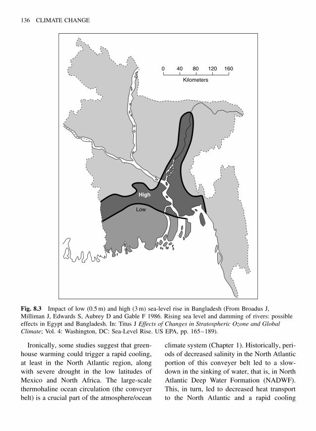
136 CLIMATE CHANGE
0 40 80
Kilometers
120 160
High
Low
Fig. 8.3 Impact of low (0.5 m) and high (3 m) sea-level rise in Bangladesh (From Broadus J,Milliman J, Edwards S, Aubrey D and Gable F 1986. Rising sea level and damming of rivers: possibleeffects in Egypt and Bangladesh. In: Titus J Effects of Changes in Stratospheric Ozone and GlobalClimate; Vol. 4: Washington, DC: Sea-Level Rise. US EPA, pp. 165–189).
Ironically, some studies suggest that green-house warming could trigger a rapid cooling,at least in the North Atlantic region, alongwith severe drought in the low latitudes ofMexico and North Africa. The large-scalethermohaline ocean circulation (the conveyerbelt) is a crucial part of the atmosphere/ocean
climate system (Chapter 1). Historically, peri-ods of decreased salinity in the North Atlanticportion of this conveyer belt led to a slow-down in the sinking of water, that is, in NorthAtlantic Deep Water Formation (NADWF).This, in turn, led to decreased heat transportto the North Atlantic and a rapid cooling

CLIMATE CHANGE AND THE MARINE ENVIRONMENT 137
Box 8.2 Decadal oceanographic oscillations
Changes resulting from natural cycles can provide information on how the Earth and humansmay respond to anthropogenic greenhouse warming. A number of natural periodic cycleslink the atmosphere and the ocean and greatly influence regional and even global climate.Cycles on periods of decades or so (decadal oscillations) alter the transport of heat andgreenhouse gases from the surface to the deep ocean or between the ocean surface and theatmosphere, affect regional evaporation and precipitation patterns, and alter the productivityof plankton, invertebrate, and fish populations. Oscillation-induced changes in drought andflood affect many human activities, particularly fisheries, forestry, and agriculture. Globalclimate change could alter the frequency and the intensity of these periodic events.
The best-known cycle is the El Nino Southern Oscillation (ENSO) – a naturally occurringcyclic change in ocean currents and heat transport in the Equatorial Pacific Ocean (NOAA2002). ENSO is an alternation between a high atmospheric pressure center in the EasternPacific and a low-pressure center over Indonesia and Northern Australia. In normal periods,this pressure difference drives trade winds from east to west along the Equator (Plate 7a). Thisforces warm water to pile up (sea level actually increases by about 40 cm) in the west anddepresses the thermocline (the depth where warm water above transits to more colder waterbelow) to about 200 m deep. The warm water and evaporation results in heavy rains in theWestern Pacific and dry air over South America. Also, along the west coast of South America,water is driven offshore and replaced by the upwelling of cool nutrient-rich deep water.
In contrast, in El Nino periods, the east–west pressure difference becomes low and thetrade winds weaken in the Western Pacific. The warm water piled up in the Western Pacificnow flows back toward the east and subsurface (Kelvin) waves travel across the Pacific todepress the thermocline off South America (Plate 7b). The result is a general warming andincrease in precipitation in the Central to Eastern Pacific and dry conditions in the west.La Nina is the cold counterpart of El Nino – the other extreme of the ENSO cycle wheresea-surface temperatures in the tropical Pacific drop below normal (Plate 7c).
During the past 5,000 years, ENSO events occurred on average once or twice per decade,but since the mid-1970s, they have occurred more often and persisted longer (Rodbellet al. 1999). Some scientists believe the increasing frequency and intensity of the ENSOis a result of anthropogenic global greenhouse warming (Trenberth and Hoar 1996). Somechanges associated with El Nino include reduced productivity of the giant kelp (seaweed)in California, increased diseases in marine organisms, coral bleaching, and release of largequantities of CO2 from the Central Pacific into the atmosphere. The economic cost fromfloods, hurricanes, drought, and fire as a result of the 1982 to 1983 ENSO is estimated at$8.1 billion (UCAR/NOAA 1994).
In the North Atlantic region, a decadal scale oscillation occurs known as the North AtlanticOscillation (NAO). In a high NAO state, a high-pressure center near the Azores (west ofPortugal) and a low-pressure center in the North Atlantic near Greenland and Iceland createwinds that blow from North America to Europe. In a low NAO cycle, the Icelandic lowpressure moves south off Newfoundland and a high pressure forms over Northern Greenland.
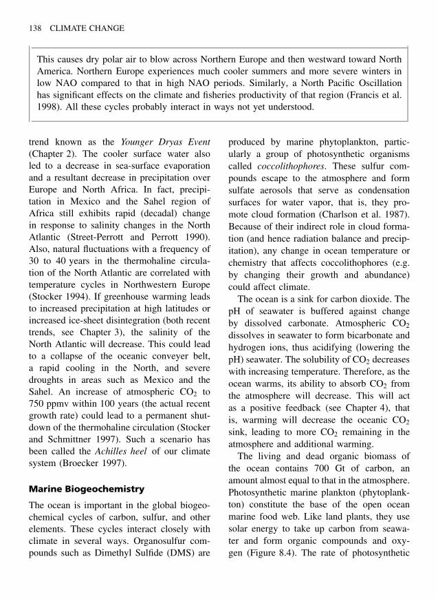
138 CLIMATE CHANGE
This causes dry polar air to blow across Northern Europe and then westward toward NorthAmerica. Northern Europe experiences much cooler summers and more severe winters inlow NAO compared to that in high NAO periods. Similarly, a North Pacific Oscillationhas significant effects on the climate and fisheries productivity of that region (Francis et al.1998). All these cycles probably interact in ways not yet understood.
trend known as the Younger Dryas Event(Chapter 2). The cooler surface water alsoled to a decrease in sea-surface evaporationand a resultant decrease in precipitation overEurope and North Africa. In fact, precipi-tation in Mexico and the Sahel region ofAfrica still exhibits rapid (decadal) changein response to salinity changes in the NorthAtlantic (Street-Perrott and Perrott 1990).Also, natural fluctuations with a frequency of30 to 40 years in the thermohaline circula-tion of the North Atlantic are correlated withtemperature cycles in Northwestern Europe(Stocker 1994). If greenhouse warming leadsto increased precipitation at high latitudes orincreased ice-sheet disintegration (both recenttrends, see Chapter 3), the salinity of theNorth Atlantic will decrease. This could leadto a collapse of the oceanic conveyer belt,a rapid cooling in the North, and severedroughts in areas such as Mexico and theSahel. An increase of atmospheric CO2 to750 ppmv within 100 years (the actual recentgrowth rate) could lead to a permanent shut-down of the thermohaline circulation (Stockerand Schmittner 1997). Such a scenario hasbeen called the Achilles heel of our climatesystem (Broecker 1997).
Marine Biogeochemistry
The ocean is important in the global biogeo-chemical cycles of carbon, sulfur, and otherelements. These cycles interact closely withclimate in several ways. Organosulfur com-pounds such as Dimethyl Sulfide (DMS) are
produced by marine phytoplankton, partic-ularly a group of photosynthetic organismscalled coccolithophores. These sulfur com-pounds escape to the atmosphere and formsulfate aerosols that serve as condensationsurfaces for water vapor, that is, they pro-mote cloud formation (Charlson et al. 1987).Because of their indirect role in cloud forma-tion (and hence radiation balance and precip-itation), any change in ocean temperature orchemistry that affects coccolithophores (e.g.by changing their growth and abundance)could affect climate.
The ocean is a sink for carbon dioxide. ThepH of seawater is buffered against changeby dissolved carbonate. Atmospheric CO2
dissolves in seawater to form bicarbonate andhydrogen ions, thus acidifying (lowering thepH) seawater. The solubility of CO2 decreaseswith increasing temperature. Therefore, as theocean warms, its ability to absorb CO2 fromthe atmosphere will decrease. This will actas a positive feedback (see Chapter 4), thatis, warming will decrease the oceanic CO2
sink, leading to more CO2 remaining in theatmosphere and additional warming.
The living and dead organic biomass ofthe ocean contains 700 Gt of carbon, anamount almost equal to that in the atmosphere.Photosynthetic marine plankton (phytoplank-ton) constitute the base of the open oceanmarine food web. Like land plants, they usesolar energy to take up carbon from seawa-ter and form organic compounds and oxy-gen (Figure 8.4). The rate of photosynthetic
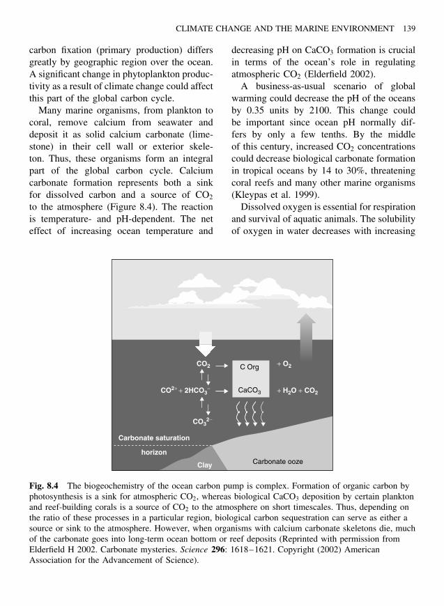
CLIMATE CHANGE AND THE MARINE ENVIRONMENT 139
carbon fixation (primary production) differsgreatly by geographic region over the ocean.A significant change in phytoplankton produc-tivity as a result of climate change could affectthis part of the global carbon cycle.
Many marine organisms, from plankton tocoral, remove calcium from seawater anddeposit it as solid calcium carbonate (lime-stone) in their cell wall or exterior skele-ton. Thus, these organisms form an integralpart of the global carbon cycle. Calciumcarbonate formation represents both a sinkfor dissolved carbon and a source of CO2
to the atmosphere (Figure 8.4). The reactionis temperature- and pH-dependent. The neteffect of increasing ocean temperature and
decreasing pH on CaCO3 formation is crucialin terms of the ocean’s role in regulatingatmospheric CO2 (Elderfield 2002).
A business-as-usual scenario of globalwarming could decrease the pH of the oceansby 0.35 units by 2100. This change couldbe important since ocean pH normally dif-fers by only a few tenths. By the middleof this century, increased CO2 concentrationscould decrease biological carbonate formationin tropical oceans by 14 to 30%, threateningcoral reefs and many other marine organisms(Kleypas et al. 1999).
Dissolved oxygen is essential for respirationand survival of aquatic animals. The solubilityof oxygen in water decreases with increasing
CO2 + O2
+ H2O + CO2CO2+ + 2HCO3−
Clay
Carbonate saturation
horizon
CO32−
C Org
Carbonate ooze
CaCO3
Fig. 8.4 The biogeochemistry of the ocean carbon pump is complex. Formation of organic carbon byphotosynthesis is a sink for atmospheric CO2, whereas biological CaCO3 deposition by certain planktonand reef-building corals is a source of CO2 to the atmosphere on short timescales. Thus, depending onthe ratio of these processes in a particular region, biological carbon sequestration can serve as either asource or sink to the atmosphere. However, when organisms with calcium carbonate skeletons die, muchof the carbonate goes into long-term ocean bottom or reef deposits (Reprinted with permission fromElderfield H 2002. Carbonate mysteries. Science 296: 1618–1621. Copyright (2002) AmericanAssociation for the Advancement of Science).
140 CLIMATE CHANGE
temperature and salinity. Also, oxygen tendsto become depleted by bacterial respirationin waters loaded with organic material. Somecoastal waters may experience oxygen deple-tion as a result of greenhouse warming. Forexample, discharge of organic material andfreshwater from the Mississippi River createsa large (16,500 km2) zone of hypoxia (lowoxygen) below the surface mixed layer of theNorthern Gulf of Mexico. Model simulationsfor a doubled-CO2 climate predict a 30 to 60%decrease in oxygen below this mixed layer,leading to enlargement of the oxygen-depleted(dead) zone of the Gulf of Mexico (Justic’et al. 1996).
Finally, research is only beginning toexplore the complicated interactions betweenglobal warming, oceanic circulation, biota,and carbon cycle feedbacks. According tomodel simulations, the North Atlantic DeepWater Formation will weaken, and at highlevels of atmospheric CO2, it will collapse.Weakened heat transport to deep water willresult in warmer surface water and thus lowerCO2 solubility. The net effect of this feed-back will be an additional increase in atmo-spheric CO2 of 4% by 2100 and 20% by 2500,although a range of possible scenarios couldoccur (Joos et al. 1999).
Marine Ecosystems
Plankton
Each plankton species has its own optimalenvironmental conditions for photosynthesis,growth, and reproduction. A 2 ◦C rise in aver-age ocean surface temperature would proba-bly bring about major shifts in the abundanceand distribution of individual plankton species(Fogg 1991) and affect the abundance of her-bivores and fish further up the food web. Inoffshore waters of Southern California, mea-surements from 1951 to 1993 indicate an 80%
decrease in the abundance of animal plank-ton concurrent with a rise in surface watertemperatures of 1.2 to 1.6 ◦C (Roemmich andMcGowan 1995).
Fish
Global warming could devastate some of theworld’s most productive fisheries. Four pri-mary factors control fish populations: thenumber of fish spawning, the availability offood for young fish larvae, the physical trans-port of larvae in the water, and predationon larvae and juveniles. All these processesare affected by temperature. The availabilityof plankton food is critical to young devel-oping larvae, and fisheries yield decreasesexponentially with decreases in plankton pro-duction (Figure 8.5). This means that a smalldecrease in plankton production, for example,in response to climatic change, could lead toa large decrease in fish production.
Since the success of fish populations isclosely linked to water temperature, it is notsurprising that most fish populations are dis-tributed regionally or globally, within a char-acteristic temperature range (thermal habitat)that can be mapped as temperature isotherms(lines of equal temperature). Changes in oceantemperature are likely to lead to changes infish populations. Generally, increasing tem-peratures are favorable to fish stocks that existat the higher-latitude end of their temperaturerange and detrimental to stocks that live at thelower-latitude end of their temperature range.
Although overfishing can devastate fishstocks, major changes in fish populationsalso often result from changing environmen-tal conditions including water temperature.The catch from several widely separated pop-ulations of sardines in the Pacific increasesduring periods of cold water and decreasesdramatically during periods of warm water(Figure 8.6). Norwegian scientists have also
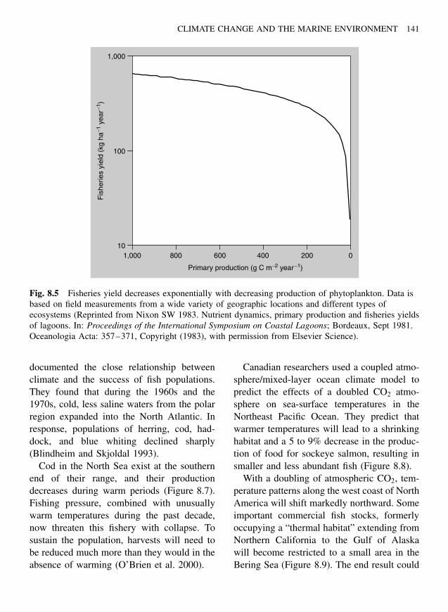
CLIMATE CHANGE AND THE MARINE ENVIRONMENT 141
1,000
100
101,000 800 600 400
Primary production (g C m−2 year−1)
Fis
herie
s yi
eld
(kg
ha−1
yea
r−1)
200 0
Fig. 8.5 Fisheries yield decreases exponentially with decreasing production of phytoplankton. Data isbased on field measurements from a wide variety of geographic locations and different types ofecosystems (Reprinted from Nixon SW 1983. Nutrient dynamics, primary production and fisheries yieldsof lagoons. In: Proceedings of the International Symposium on Coastal Lagoons; Bordeaux, Sept 1981.Oceanologia Acta: 357–371, Copyright (1983), with permission from Elsevier Science).
documented the close relationship betweenclimate and the success of fish populations.They found that during the 1960s and the1970s, cold, less saline waters from the polarregion expanded into the North Atlantic. Inresponse, populations of herring, cod, had-dock, and blue whiting declined sharply(Blindheim and Skjoldal 1993).
Cod in the North Sea exist at the southernend of their range, and their productiondecreases during warm periods (Figure 8.7).Fishing pressure, combined with unusuallywarm temperatures during the past decade,now threaten this fishery with collapse. Tosustain the population, harvests will need tobe reduced much more than they would in theabsence of warming (O’Brien et al. 2000).
Canadian researchers used a coupled atmo-sphere/mixed-layer ocean climate model topredict the effects of a doubled CO2 atmo-sphere on sea-surface temperatures in theNortheast Pacific Ocean. They predict thatwarmer temperatures will lead to a shrinkinghabitat and a 5 to 9% decrease in the produc-tion of food for sockeye salmon, resulting insmaller and less abundant fish (Figure 8.8).
With a doubling of atmospheric CO2, tem-perature patterns along the west coast of NorthAmerica will shift markedly northward. Someimportant commercial fish stocks, formerlyoccupying a “thermal habitat” extending fromNorthern California to the Gulf of Alaskawill become restricted to a small area in theBering Sea (Figure 8.9). The end result could
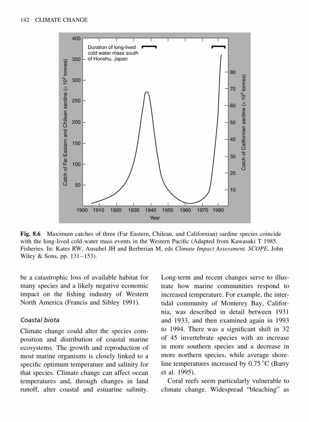
142 CLIMATE CHANGE
400
350
300
250
200
150
100
50
1900 1910 1920 1930 1940
Year
Cat
ch o
f Far
Eas
tern
and
Chi
lean
sar
dine
(×
103
tonn
es)
Cat
ch o
f Cal
iforn
ian
sard
ine
(× 1
03 to
nnes
)
1950 1960 1970 1980
80
70
60
50
40
30
20
10
Duration of long-livedcold water mass southof Honshu, Japan
Fig. 8.6 Maximum catches of three (Far Eastern, Chilean, and Californian) sardine species coincidewith the long-lived cold-water mass events in the Western Pacific (Adapted from Kawasaki T 1985.Fisheries. In: Kates RW, Ausubel JH and Berberian M, eds Climate Impact Assessment. SCOPE. JohnWiley & Sons, pp. 131–153).
be a catastrophic loss of available habitat formany species and a likely negative economicimpact on the fishing industry of WesternNorth America (Francis and Sibley 1991).
Coastal biota
Climate change could alter the species com-position and distribution of coastal marineecosystems. The growth and reproduction ofmost marine organisms is closely linked to aspecific optimum temperature and salinity forthat species. Climate change can affect oceantemperatures and, through changes in landrunoff, alter coastal and estuarine salinity.
Long-term and recent changes serve to illus-trate how marine communities respond toincreased temperature. For example, the inter-tidal community of Monterey Bay, Califor-nia, was described in detail between 1931and 1933, and then examined again in 1993to 1994. There was a significant shift in 32of 45 invertebrate species with an increasein more southern species and a decrease inmore northern species, while average shore-line temperatures increased by 0.75 ◦C (Barryet al. 1995).
Coral reefs seem particularly vulnerable toclimate change. Widespread “bleaching” as
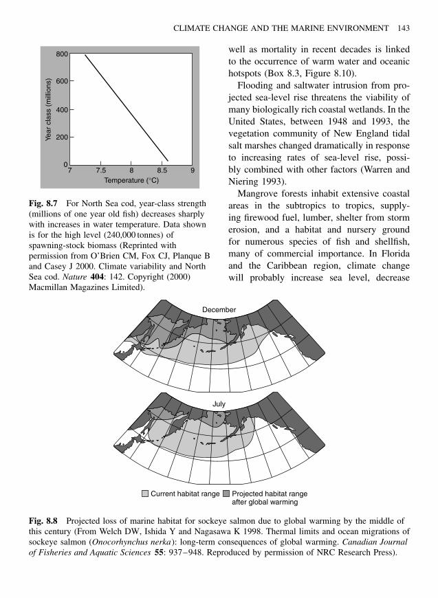
CLIMATE CHANGE AND THE MARINE ENVIRONMENT 143
800
600
400
200
07 7.5 8
Temperature (°C)
Year
cla
ss (
mill
ions
)
8.5 9
Fig. 8.7 For North Sea cod, year-class strength(millions of one year old fish) decreases sharplywith increases in water temperature. Data shownis for the high level (240,000 tonnes) ofspawning-stock biomass (Reprinted withpermission from O’Brien CM, Fox CJ, Planque Band Casey J 2000. Climate variability and NorthSea cod. Nature 404: 142. Copyright (2000)Macmillan Magazines Limited).
well as mortality in recent decades is linkedto the occurrence of warm water and oceanichotspots (Box 8.3, Figure 8.10).
Flooding and saltwater intrusion from pro-jected sea-level rise threatens the viability ofmany biologically rich coastal wetlands. In theUnited States, between 1948 and 1993, thevegetation community of New England tidalsalt marshes changed dramatically in responseto increasing rates of sea-level rise, possi-bly combined with other factors (Warren andNiering 1993).
Mangrove forests inhabit extensive coastalareas in the subtropics to tropics, supply-ing firewood fuel, lumber, shelter from stormerosion, and a habitat and nursery groundfor numerous species of fish and shellfish,many of commercial importance. In Floridaand the Caribbean region, climate changewill probably increase sea level, decrease
December
July
Current habitat range Projected habitat rangeafter global warming
Fig. 8.8 Projected loss of marine habitat for sockeye salmon due to global warming by the middle ofthis century (From Welch DW, Ishida Y and Nagasawa K 1998. Thermal limits and ocean migrations ofsockeye salmon (Onocorhynchus nerka): long-term consequences of global warming. Canadian Journalof Fisheries and Aquatic Sciences 55: 937–948. Reproduced by permission of NRC Research Press).
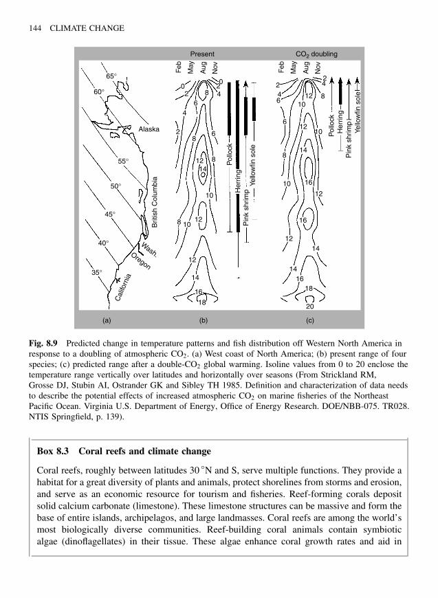
144 CLIMATE CHANGE
65°
60°
55°
45°
35°
Cal
iforn
ia
40°
50°
Alaska
Oregon
Wash.
Brit
ish
Col
umbi
a
02 8 4
4
20 2
6
28
6
1214
8
10
8 1012
12
14
16
18
Feb
May
Aug
Nov Feb
May
Aug
Nov
Present CO2 doubling
Pol
lock
Pol
lock
Her
ring
Her
ring
Pin
k sh
rimp
Pin
k sh
rimp
Yello
wfin
sol
e
Yello
wfin
sol
e46
24
81210
612
10
148
10 16
12
16
1214
1416
18
20
(a) (b) (c)
Fig. 8.9 Predicted change in temperature patterns and fish distribution off Western North America inresponse to a doubling of atmospheric CO2. (a) West coast of North America; (b) present range of fourspecies; (c) predicted range after a double-CO2 global warming. Isoline values from 0 to 20 enclose thetemperature range vertically over latitudes and horizontally over seasons (From Strickland RM,Grosse DJ, Stubin AI, Ostrander GK and Sibley TH 1985. Definition and characterization of data needsto describe the potential effects of increased atmospheric CO2 on marine fisheries of the NortheastPacific Ocean. Virginia U.S. Department of Energy, Office of Energy Research. DOE/NBB-075. TR028.NTIS Springfield, p. 139).
Box 8.3 Coral reefs and climate change
Coral reefs, roughly between latitudes 30 ◦N and S, serve multiple functions. They provide ahabitat for a great diversity of plants and animals, protect shorelines from storms and erosion,and serve as an economic resource for tourism and fisheries. Reef-forming corals depositsolid calcium carbonate (limestone). These limestone structures can be massive and form thebase of entire islands, archipelagos, and large landmasses. Coral reefs are among the world’smost biologically diverse communities. Reef-building coral animals contain symbioticalgae (dinoflagellates) in their tissue. These algae enhance coral growth rates and aid in
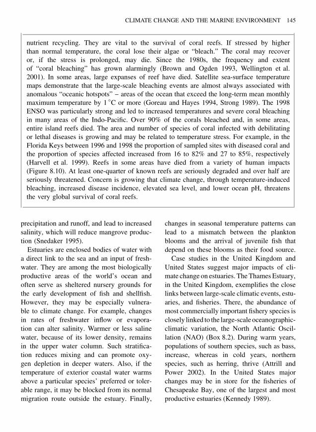
CLIMATE CHANGE AND THE MARINE ENVIRONMENT 145
nutrient recycling. They are vital to the survival of coral reefs. If stressed by higherthan normal temperature, the coral lose their algae or “bleach.” The coral may recoveror, if the stress is prolonged, may die. Since the 1980s, the frequency and extentof “coral bleaching” has grown alarmingly (Brown and Ogden 1993, Wellington et al.2001). In some areas, large expanses of reef have died. Satellite sea-surface temperaturemaps demonstrate that the large-scale bleaching events are almost always associated withanomalous “oceanic hotspots” – areas of the ocean that exceed the long-term mean monthlymaximum temperature by 1 ◦C or more (Goreau and Hayes 1994, Strong 1989). The 1998ENSO was particularly strong and led to increased temperatures and severe coral bleachingin many areas of the Indo-Pacific. Over 90% of the corals bleached and, in some areas,entire island reefs died. The area and number of species of coral infected with debilitatingor lethal diseases is growing and may be related to temperature stress. For example, in theFlorida Keys between 1996 and 1998 the proportion of sampled sites with diseased coral andthe proportion of species affected increased from 16 to 82% and 27 to 85%, respectively(Harvell et al. 1999). Reefs in some areas have died from a variety of human impacts(Figure 8.10). At least one-quarter of known reefs are seriously degraded and over half areseriously threatened. Concern is growing that climate change, through temperature-inducedbleaching, increased disease incidence, elevated sea level, and lower ocean pH, threatensthe very global survival of coral reefs.
precipitation and runoff, and lead to increasedsalinity, which will reduce mangrove produc-tion (Snedaker 1995).
Estuaries are enclosed bodies of water witha direct link to the sea and an input of fresh-water. They are among the most biologicallyproductive areas of the world’s ocean andoften serve as sheltered nursery grounds forthe early development of fish and shellfish.However, they may be especially vulnera-ble to climate change. For example, changesin rates of freshwater inflow or evapora-tion can alter salinity. Warmer or less salinewater, because of its lower density, remainsin the upper water column. Such stratifica-tion reduces mixing and can promote oxy-gen depletion in deeper waters. Also, if thetemperature of exterior coastal water warmsabove a particular species’ preferred or toler-able range, it may be blocked from its normalmigration route outside the estuary. Finally,
changes in seasonal temperature patterns canlead to a mismatch between the planktonblooms and the arrival of juvenile fish thatdepend on these blooms as their food source.
Case studies in the United Kingdom andUnited States suggest major impacts of cli-mate change on estuaries. The Thames Estuary,in the United Kingdom, exemplifies the closelinks between large-scale climatic events, estu-aries, and fisheries. There, the abundance ofmost commercially important fishery species isclosely linked to the large-scale oceanographic-climatic variation, the North Atlantic Oscil-lation (NAO) (Box 8.2). During warm years,populations of southern species, such as bass,increase, whereas in cold years, northernspecies, such as herring, thrive (Attrill andPower 2002). In the United States majorchanges may be in store for the fisheries ofChesapeake Bay, one of the largest and mostproductive estuaries (Kennedy 1989).
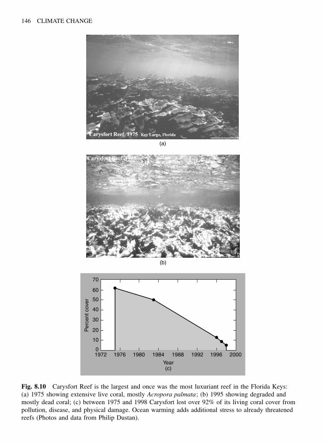
146 CLIMATE CHANGE
70
60
50
40
30
20
10
01972 1976 1980 1984 1988
Year
Per
cent
cov
er
(c)
1992 1996 2000
(a)
(b)
Fig. 8.10 Carysfort Reef is the largest and once was the most luxuriant reef in the Florida Keys:(a) 1975 showing extensive live coral, mostly Acropora palmata; (b) 1995 showing degraded andmostly dead coral; (c) between 1975 and 1998 Carysfort lost over 92% of its living coral cover frompollution, disease, and physical damage. Ocean warming adds additional stress to already threatenedreefs (Photos and data from Philip Dustan).
CLIMATE CHANGE AND THE MARINE ENVIRONMENT 147
Marine mammals
Many marine mammals are threatened byhabitat destruction and fragmentation. Globalwarming will put additional pressure on theirability to survive (Harwood 2001). Manymarine mammals serve as keystone speciesin the food web. Depletion of their numberscan result in a cascade of changing abundancein other species. The extent of sea ice hasdeclined and will probably decline another40% or more by 2100 (Hadley Centre 2002).This will shrink the available habitat ofpinnipeds (seals and sea lions) and polarbears that rely on sea ice for resting andpupping and of cetaceans such as the bowheadwhale that rely on high levels of planktonproductivity associated with the ice edge.Earlier breakup of sea ice in Western HudsonBay may already be responsible for thedeclining condition of polar bears in thatregion (Stirling et al. 1999). However, themost threatened aquatic mammals may becertain species of seals that are endemicto inland seas and large lakes such as theCaspian Sea in Southwestern Asia and LakeBaikal in Southern Siberia. If adequate icedoes not develop, these seals will not haveenough habitat for breeding. In fact, thissituation may already be under way in theCaspian, where recent small ice areas haveled to crowding during the breeding seasonand mass mortality from disease (Kennedyet al. 2000).
Marine diseases
Environmental stress, whether from pollu-tion or from climate change, can weakenorganisms, making them more susceptible todisease. The incidence of disease in manymarine species is increasing around the world(Harvell et al. 1999). These disease out-breaks often result in mass mortalities ofmarine plants, invertebrates, and vertebrates.
For example, the pathogenic infection anddie-off of the dominant sea urchin and key-stone herbivore Diadema antillarum in theCaribbean in the 1980s led to a massive phaseshift. In the absence of herbivorous urchins,algae thrived and covered and killed the coral.The result was a shift from coral- to algal-dominated reefs. Coral reefs are also dyingfrom temperature stress and more frequentand widespread marine diseases (Box 8.2).
An almost 25-year warming trend on theeast coast of the United States may be respon-sible for the spread of several diseases andmass mortalities in oyster populations. Also,mass mortalities of seals in recent yearsin Northern Europe resulted from infectionwith a pathogenic virus known as phocinedistemper virus. As temperatures rise, sealsspend more time on the beach as opposed tothe water and congregate in dense aggrega-tions. This sets the stage for the rapid spreadof the opportunistic pathogen (Lavigne andSchmitz 1990).
Diseases, spread through the marine envi-ronment, are not restricted to marine species.Many human pathogens such as cholera arenaturally active in coastal waters, or follow-ing introduction via sewage or storm wateroutfalls, remain dormant for a period of time.Warm water may trigger them to emerge inan infectious state.
Blooms of algae, particularly toxic andundesirable species, have increased in manyregions of the world (Smayda and Shimizu1993) and seem linked to warming oceantemperatures (Epstein et al. 1994). Theseblooms are implicated in mass mortalitiesof marine mammals and fish. For example,a toxic phytoplankton (Gymnodinium catena-tum) killed 70% of the Mediterranean monkseal population on the coast of the West-ern Sahara in 1997 (Forcada et al. 1999).In addition, changing temperature and ocean
148 CLIMATE CHANGE
currents along the northwest coast of Spainare expected to lead to an increase in bloomsof the toxic single-celled algal dinoflagellatesresponsible for paralytic shellfish poisoning(Fraga and Bakun 1993).
Summary
Recent changes in the marine environment inresponse to greenhouse warming will prob-ably continue and even accelerate. Predictedchanges, by the end of this century, includethe following:
A global average sea-level rise of about 0.2to 0.7 m resulting in
• increased beach erosion and coastalflooding;
• loss of coastal ecosystems such as man-groves and wetlands;
• displacement of human populations awayfrom low-lying areas;
• saltwater intrusion into coastal aquiferwater supplies.
Possible changes in large-scale ocean circu-lation patterns:
• a possible collapse of the oceanic conveyerbelt, followed by rapid climate coolingand decreased precipitation in the Mediter-ranean and the African Sahel region;
• intensified upwelling of cool water alongthe western coasts of the Americas, South-ern Europe, and Africa.
Alteration of important oceanic biogeo-chemical cycles:
• a warming-induced decrease in the abilityof the ocean to absorb CO2;
• a decrease in bio-carbonate formation nec-essary for reef-forming corals and othermarine species;
• lower concentrations of life-supporting dis-solved oxygen in some marine waters.
Direct impacts on marine ecosystems:
• changes in the species population abun-dance of plankton that form the base of themarine food web;
• changes in the geographic distribution andspecies composition of coastal ecosystems;
• additional temperature stress on communi-ties already threatened by human impacts,for example, coral reefs and mangroves;
• decreased productivity and altered distribu-tions of fish and marine mammals.
References
Attrill MJ and Power M 2002 Climatic influence ona marine fish assemblage. Nature 417: 275–278.
Bakun A 1992 Global greenhouse effects, multi-decadal wind trends, and potential impacts oncoastal pelagic fish populations. InternationalCouncil for Exploration of the Sea Marine Sci-ence Symposium: Hydrobiological Variability inthe ICES Area 1980–1989 , Mariehamn 1991:316–325.
Barry JP, Baxter CH, Sagarin RD and Gilman SE1995 Climate-related, long-term faunal changes ina California rocky intertidal community. Science267: 672–675.
Bigg GR 1996 The Oceans and Climate. Cambridge.Cambridge University Press.
Blindheim J and Skjoldal HR 1993 Effects of climaticchange on the biomass yield of the Barents Sea,Norwegian Sea, and West Greenland large marineecosystems. In: Proceedings of the InternationalConference on Large Marine Ecosystems: Stress,Mitigation and Sustainability . Monaco, IUCN: TheWorld Conservation Union, pp. 185–198.
Broadus J, Milliman J, Edwards S, Aubrey D andGable F 1986 Rising sea level and damming ofrivers: possible effects in Egypt and Bangladesh.
CLIMATE CHANGE AND THE MARINE ENVIRONMENT 149
In: Titus J, ed. Effects of Changes in StratosphericOzone and Global Climate; Vol. 4: Sea Level Rise.Washington, DC: US EPA, pp. 165–189.
Broecker WS 1997 Thermohaline circulation, theAchilles heel of our climate system: will man-made CO2 upset the current balance? Science 278:1582–1588.
Bromwich D 1995 Ice sheets and sea level. Nature373: 18,19.
Brown B and Ogden JC 1993 Coral bleaching.Scientific American January: 63–70.
Brunn P 1962 Sea level rise as a cause of shore ero-sion. Journal of Waterways and Harbors Division(ASCE) 1: 116–130.
Charlson R, Lovelock J, Andrae M and Warren S1987 Oceanic phytoplankton, atmospheric sulphur,cloud albedo and climate. Nature 326: 655–661.
Church JA and Gregory JM 2001 Changes in sealevel. In: Houghton JT, Ding Y, Griggs DJ, NoguerM, van der Linden PJ, Dai X, et al., eds Cli-mate Change 2001: The Scientific Basis. Inter-governmental Panel on Climate Change, WorkingGroup I . Cambridge: Cambridge University Press,pp. 639–693.
Elderfield H 2002 Carbonate mysteries. Science 296:1618–1621.
Epstein PR, Ford TE and Colwell R 1994 Marineecosystems. In: Health and Climate Change. TheLancet, London, pp. 14–17.
Fogg GE 1991 Changing productivity of the oceansin response to a changing climate. Annals of Botany67(Suppl. 1): 57–60.
Forcada J, Hammond P and Aguilar A 1999 Thestatus of the Mediterranean monk seal in theWestern Sahara and the implications of a massmortality. Marine Ecology Progress Series 188:249–261.
Fraga S and Bakun A 1993 Global climate changeand harmful algal blooms: the example of Gymno-dinium catenatum on the Galacian coast. In:Smayda TJ and Shimizu Y, eds Toxic Phytoplank-ton Blooms in the Sea: Proceedings of the FifthInternational Conference on Toxic Marine Phyto-plankton; Newport, Rhode Island; 28 October-1November 1991 . Amsterdam. Elsevier, pp. 59–65.
Francis RC and Sibley TH 1991 Climate changeand fisheries: what are the real issues? NorthwestEnvironmental Journal 7: 295–307.
Francis RC, Hare SR, Hollowed AB and Wooster WS1998 Effects of interdecadal climate variability on
the oceanic ecosystems of the NE Pacific. FisheriesOceanography 7: 1–21.
Goreau TJ and Hayes RL 1994 Coral Bleaching andOcean “Hot Spots”. Ambio 23(3): 176–180.
Hadley Centre 2002 Meteorological Office, UnitedKingdom http://www.meto.govt.uk/research/hadleycentre/models/modeldata.html
Harleman DRF, Bras RL, Rinaldo A and MalanotteP 2000 Blocking the tide. Civil EngineeringOctober: 52–57.
Harvell CD, Kim K, Burkholder JM, Colwell RR,Epstein PR, Grimes DJ, et al. 1999 Emergingmarine diseases-climate links and anthropogenicfactors. Science 285: 1505–1510.
Harwood J 2001 Marine mammals and their environ-ment in the twenty-first century. Journal of Mam-malogy 82(3): 630–640.
Joos F, Plattner G-K, Stocker TF, Marchal O andSchmittner A 1999 Global warming and marinecarbon cycle feedbacks on future atmospheric CO2.Science 284: 464–467.
Justic’ D, Rabalais NN and Turner RE 1996 Effectsof climate change on hypoxia in coastal waters:a doubled CO2 scenario for the northern Gulfof Mexico. Limnology and Oceanography 41:992–1003.
Kawasaki T 1985 Fisheries. In: Kates RW, AusubelJH and Berberian M, eds Climate Impact Assess-ment. SCOPE . Chichester, UK, John Wiley &Sons, pp. 131–153.
Kennedy V 1989 Potential effects of climate changeon Chesapeake Bay animals and fisheries. In: Top-ping JC, ed. Coping With Climate Change: Pro-ceedings of the Second North American Confer-ence on Preparing for Climate Change. Decem-ber 6–8, Washington, DC: The Climate Institute,pp. 509–513.
Kennedy S, Kuiken T, Jepson PD, Deaville R,Forsyth M, Barrett T, et al. 2000 Mass die-off ofCaspian seals caused by canine distemper virus.Emerging Infectious Diseases 6(6): 637–639.
Kleypas JA, Buddemeier RW, Archer D, Gattuso J-P, Langdon C and Opdyke BN 1999 Geochemicalconsequences of increased atmospheric carbondioxide on coral reefs. Science 284: 118–120.
Lavigne DM and Schmitz OJ 1990 Global warmingand increasing population densities: a prescriptionfor seal plagues. Marine Pollution Bulletin 21:280–284.
Nixon SW 1982 Nutrient dynamics, primary produc-tion and fisheries yields of lagoons. In Proceedings
150 CLIMATE CHANGE
International Symposium on Coastal Lagoons. Bor-deaux, Sept 1981. Oceanologia Acta 357–371.
El Nino 2002 National Oceanic and AtmosphericAdministration . Available from: http://www.pmel.noaa.gov/tao/elnino/nino-home.html
Nunn PD 1988 Future sea-level rise in the Pacific:Effects on selected parts of Cook Islands, Fiji, Kiri-bati, Tonga and Western Samoa. Technical Report .Suva, Fiji, School of Social and Economic Devel-opment, University of the South Pacific, p. 46.
O’Brien CM, Fox CJ, Planque B and Casey J 2000Climate variability and North Sea cod. Nature404: 142.
Peltier WR and Tushingham AM 1989 Global sealevel rise and the greenhouse effect: might they beconnected? Science 244: 806–810.
Rodbell DT, Seltzer GO, Anderson DM, Abbott MB,Enfield DB and Newman JH 1999 A similar to15,000-year record of El Nino-driven alluviationin southwestern Ecuador. Science 283: 516–520.
Roemmich D and McGowan J 1995 Climatic warm-ing and the decline of zooplankton in the CaliforniaCurrent. Science 267: 1324–1326.
Roy P and Connell J 1991 Climatic change and thefuture of atoll states. Journal of Coastal Research7(4): 1057–1075.
Smayda TJ and Shimizu Y, eds 1993 Toxic Phyto-plankton Blooms in the Sea: Proceedings of theFifth International Conference on Toxic MarinePhytoplankton; Newport, Rhode Island; 28 Octo-ber-1 November 1991 . Amsterdam, Elsevier.
Snedaker SC 1995 Mangroves and climate change inthe Florida and Caribbean Region: scenarios andhypotheses. Hydrobiologia 295: 43–49.
Stocker TF 1994 The variable ocean. Nature 367:221–222.
Stocker TF and Schmittner A 1997 Influence of CO2
emission rates on the stability of the thermohalinecirculation. Nature 388: 862–865.
Stirling I, Lunn N and Iacozza J 1999 Long-termtrends in the population ecology of polar bears inwestern Hudson Bay in relation to climate change.Arctic 52: 294–306.
Street-Perrott FA and Perrott RA 1990 Abrupt climatefluctuations in the tropics. The influence of Atlanticocean circulation. Nature 343: 607–612.
Strickland RM, Grosse DJ, Stubin AI, Ostrander GKand Sibley TH 1985 Definition and characteriza-
tion of data needs to describe the potential effectsof increased atmospheric CO2 on marine fisheriesof the Northeast Pacific Ocean . Virginia, U.S.Department of Energy, Office of Energy Research.DOE/NBB-075. TR028. NTIS Springfield, p. 78.
Strong AE 1989 Greater global warming revealedby satellite-derived sea-surface temperature trends.Nature 338: 642–645.
Titus JG 1986 Greenhouse effect, sea level rise, andcoastal zone management. Coastal Zone Manage-ment Journal 14(3): 147–171.
Titus JG and Narayanan V 1996 The risk of sea levelrise. Climatic Change 33: 151–212.
Titus JG, Park RA, Leatherman SP, Weggel JR,Greene MS, Mausel PW, et al. 1991 Greenhouseeffect and sea level rise: the cost of holding backthe sea. Coastal Management 19: 171–204.
Trenberth KE and Hoar TJ 1996 The 1990–1995El Nino-Southern Oscillation event: Longeston record. Geophysical Research Letters 23(1):57–60.
UCAR/NOAA 1994 University Center for Atmo-spheric Research and National Oceanic and Atmo-spheric Administration. Boulder Colorado andWashington, DC. http://www.ucar.edu/ucar/index.html
UNEP 2002 Available from: http://www.grida.no/climate/vital/impacts.htm
Warren RS and Niering WA 1993 Vegetation changeon a Northeast tidal marsh: interaction of sea-levelrise and marsh accretion. Ecology 74(1): 96–103.
Weaver AJ 1993 The oceans and global warming.Nature 364: 192–193.
Welch DW, Ishida Y and Nagasawa K 1998 Thermallimits and ocean migrations of sockeye salmon(Onocorhynchus nerka): long-term consequencesof global warming. Canadian Journal of Fisheriesand Aquatic Sciences 55: 937–948.
Wellington GM, Glynn PW, Strong AE, NavarreteSA, Wieters E and Hubbard D 2001 Crisis on coralreefs linked to climate change. EOS, Transactionsof the American Geophysical Union 82(1): 1–5.
Williams PB 1985 An overview of the impact ofaccelerated sea level rise on San Francisco Bay.Report on Project 256. December 20 . San Fran-cisco, Phillip Williams & Associates.
WWF 2002 Available from: http://www.panda.org/climate/

SECTION III
Human Dimensions of Climate Change
151

This Page Intentionally Left Blank
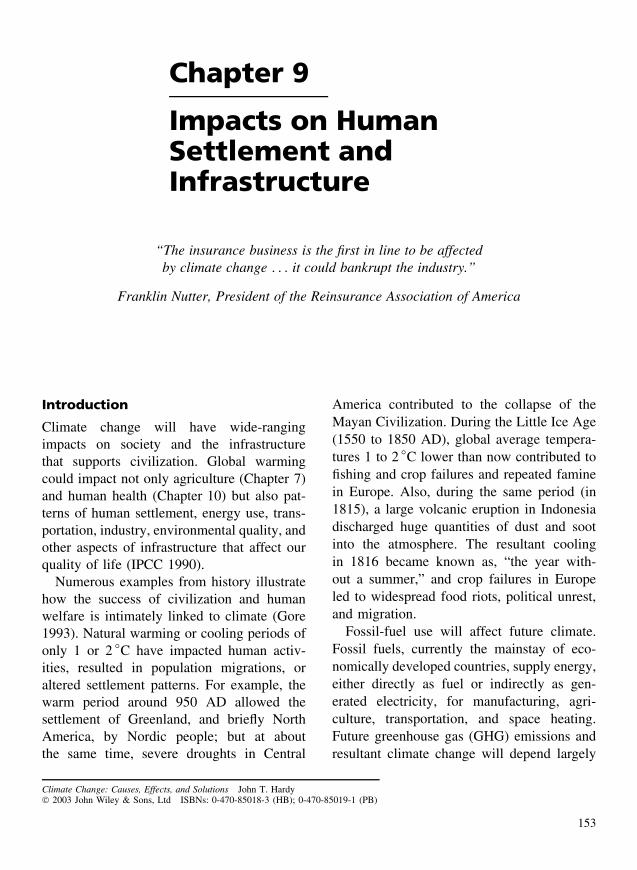
Chapter 9
Impacts on HumanSettlement andInfrastructure
“The insurance business is the first in line to be affectedby climate change . . . it could bankrupt the industry.”
Franklin Nutter, President of the Reinsurance Association of America
Introduction
Climate change will have wide-rangingimpacts on society and the infrastructurethat supports civilization. Global warmingcould impact not only agriculture (Chapter 7)and human health (Chapter 10) but also pat-terns of human settlement, energy use, trans-portation, industry, environmental quality, andother aspects of infrastructure that affect ourquality of life (IPCC 1990).
Numerous examples from history illustratehow the success of civilization and humanwelfare is intimately linked to climate (Gore1993). Natural warming or cooling periods ofonly 1 or 2 ◦C have impacted human activ-ities, resulted in population migrations, oraltered settlement patterns. For example, thewarm period around 950 AD allowed thesettlement of Greenland, and briefly NorthAmerica, by Nordic people; but at aboutthe same time, severe droughts in Central
America contributed to the collapse of theMayan Civilization. During the Little Ice Age(1550 to 1850 AD), global average tempera-tures 1 to 2 ◦C lower than now contributed tofishing and crop failures and repeated faminein Europe. Also, during the same period (in1815), a large volcanic eruption in Indonesiadischarged huge quantities of dust and sootinto the atmosphere. The resultant coolingin 1816 became known as, “the year with-out a summer,” and crop failures in Europeled to widespread food riots, political unrest,and migration.
Fossil-fuel use will affect future climate.Fossil fuels, currently the mainstay of eco-nomically developed countries, supply energy,either directly as fuel or indirectly as gen-erated electricity, for manufacturing, agri-culture, transportation, and space heating.Future greenhouse gas (GHG) emissions andresultant climate change will depend largely
Climate Change: Causes, Effects, and Solutions John T. Hardy 2003 John Wiley & Sons, Ltd ISBNs: 0-470-85018-3 (HB); 0-470-85019-1 (PB)
153

154 CLIMATE CHANGE
on future rates of fossil-fuel consumption.Many complex and interacting factors deter-mine the consumption rate of fossil fuels.Demand is a result of population growth rate,availability of fossil fuel, energy efficiency,conservation measures, use of nonfossil en-ergy sources, general industrial productivity,and energy policy. All these factors will affectfossil-fuel utilization rates and future climate.
Future climate, in turn, will affect fossil-fuel use. As climate changes, patterns ofenergy use will change. Humans living in coldclimates require large quantities of energy forspace heating of residential and commercialbuildings. These requirements will decreasein response to warmer winters. In warm cli-mates, energy is needed for air condition-ing, and in arid regions, irrigated agriculturerequires energy for pumping water. Energydemand for these activities could increase.
The impacts of climate change on humansettlement patterns and infrastructure will dif-fer regionally and could range from insignif-icant to catastrophic. The costs of mitigatingthese impacts will vary greatly (Chapters 11and 12), but are likely to be felt mostby developing nations. Important links existbetween global climate, extreme climateevents, energy use, environmental quality,human settlement patterns, and the transporta-tion and industrial infrastructure.
Energy
The effects of energy use on climate
The United Nations Framework Conventionon Climate Change (UNFCCC 2002) calls for“stabilization of greenhouse gas concentra-tions in the atmosphere at a level that wouldprevent dangerous anthropogenic interferencewith the climate system. . . .” Can this goal bemet? The actual level at which atmosphericCO2 stabilization is achieved will depend on
the product of several factors, known togetheras the Kaya identity (Hoffert et al. 1998):
Mc = N(GDP/N)(E/GDP)(C/E);
whereMc = CO2 emitted from fossil-fuel
combustionN = population
GDP = gross domestic productE/GDP = energy intensity in W year $−1
C/E = carbon intensity = the weightedaverage of the carbon-to-energyemission factors of all energysources in kg C W−1 year−1.
Thus, global 1990 fossil-fuel CO2 emis-sions can be estimated as
5.3 × 10⁹ persons × 4,100$ per person year−1
× 0.49 W year $−1 × 0.56 kg C W−1year−1
= 6 × 10¹² kg C (6.0 gigatons of carbon)
The level of atmospheric CO2 stabiliza-tion that can be achieved in this century willdepend on all these factors (Hoffert et al.1998). The IPCC developed a number ofpossible GHG emission scenarios based onsocioeconomic projections. The business asusual scenario (IS92a) assumes current ratesof population and economic growth with nonew climate-change policies. On the basisof such a scenario, population and GDP percapita will increase, while energy intensityand carbon intensity should decrease (i.e.improve) (Figure 9.1). Nevertheless, despiteimprovement in these last two factors, therate of atmospheric CO2 emissions will dou-ble by 2050 and more than triple by 2100(Figure 9.2a). To meet the economic assump-tions of “business as usual,” total power willneed to increase greatly during this century.In the developing world, because of the pro-jected rapid growth rate in energy use, achiev-able increases in energy efficiency will have
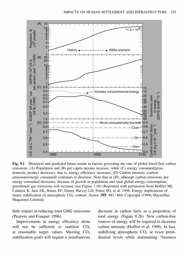
IMPACTS ON HUMAN SETTLEMENT AND INFRASTRUCTURE 155
15
10865432
13020
1086432
10.60.80.60.50.4
0.3
0.2
1.00.90.8
0.7
0.6
0.5
0.41900 2000 2100
1215202530
40506070800.90.8
0.7
0.6
0.5
0.4
History IS92a scenario
Includes noncommerical energy
11.3 × 10⁹
Wood (unsustainably burned)
Coal
Oil
Gas
(A)
(B)
(C)
(D)
Pop
ulat
ion,
N(1
09 pe
ople
)G
DP
/N (
103
US
$pe
r pe
rson
yea
r−1)
(199
0)E
/GD
P (
W y
ear−1
per
US
$)
(199
0)C
/E (
Gt C
TW
−1 y
ear−1
)
Eco
nom
ic y
ield
of e
nerg
y,G
DP
/E (
$ kW
−1 h
−1)
Car
bon
emis
sion
fact
or,
C/E
(kg
C W
−1 y
ear−1
)
Fig. 9.1 Historical and predicted future trends in factors governing the rate of global fossil-fuel carbonemissions. (A) Population and (B) per capita income increase, while (C) energy consumed/grossdomestic product decreases, that is, energy efficiency increases. (D) Carbon intensity (carbonemissions/energy consumed) continues to decrease. Note that in (D), although carbon emissions perenergy consumed decreases, because of growth in population and total global energy consumption,greenhouse gas emissions will increase (see Figure 1.10) (Reprinted with permission from Hoffert MI,Caldeira K, Jain AK, Haites EF, Danny Harvey LD, Potter SD, et al. 1998. Energy implications offuture stabilization of atmospheric CO2 content. Nature 395: 881–884. Copyright (1998) MacmillanMagazines Limited).
little impact in reducing total GHG emissions(Pearson and Fouquet 1996).
Improvements in energy efficiency alonewill not be sufficient to stabilize CO2
at reasonable target values. Meeting CO2
stabilization goals will require a simultaneous
decrease in carbon fuels as a proportion oftotal energy (Figure 9.2b). New carbon-freesources of energy will be required to decreasecarbon intensity (Hoffert et al. 1998). In fact,stabilizing atmospheric CO2 at twice prein-dustrial levels while maintaining “business
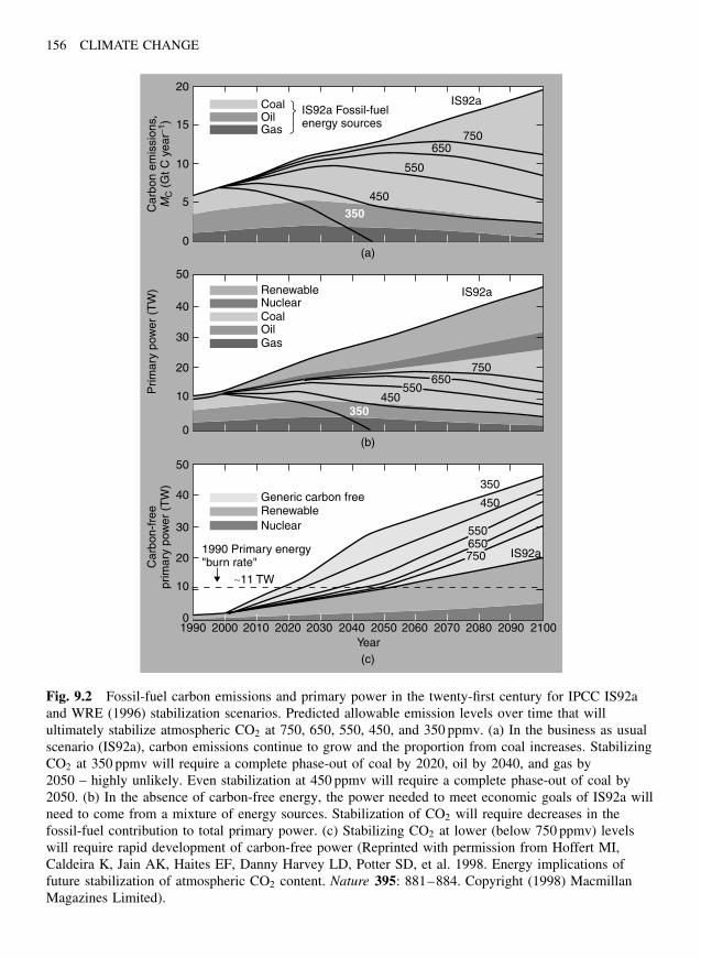
156 CLIMATE CHANGE
20
(a)
(b)
(c)
15
10
5
50
40
30
20
10
50
40
30
20
10
01990 2000 2010 2020 2030 2040
Year2050 2060 2070 2080 2090 2100
0
0
Coal
Renewable
Generic carbon freeRenewableNuclear
NuclearCoalOilGas
OilGas
IS92a Fossil-fuelenergy sources
IS92a
IS92a
750
350
450
550650750 IS92a
650550
450
750650
550
450
350
350
1990 Primary energy"burn rate"
∼11 TW
Car
bon
emis
sion
s,M
C (
Gt C
yea
r−1)
Prim
ary
pow
er (
TW
)C
arbo
n-fr
eepr
imar
y po
wer
(T
W)
Fig. 9.2 Fossil-fuel carbon emissions and primary power in the twenty-first century for IPCC IS92aand WRE (1996) stabilization scenarios. Predicted allowable emission levels over time that willultimately stabilize atmospheric CO2 at 750, 650, 550, 450, and 350 ppmv. (a) In the business as usualscenario (IS92a), carbon emissions continue to grow and the proportion from coal increases. StabilizingCO2 at 350 ppmv will require a complete phase-out of coal by 2020, oil by 2040, and gas by2050 – highly unlikely. Even stabilization at 450 ppmv will require a complete phase-out of coal by2050. (b) In the absence of carbon-free energy, the power needed to meet economic goals of IS92a willneed to come from a mixture of energy sources. Stabilization of CO2 will require decreases in thefossil-fuel contribution to total primary power. (c) Stabilizing CO2 at lower (below 750 ppmv) levelswill require rapid development of carbon-free power (Reprinted with permission from Hoffert MI,Caldeira K, Jain AK, Haites EF, Danny Harvey LD, Potter SD, et al. 1998. Energy implications offuture stabilization of atmospheric CO2 content. Nature 395: 881–884. Copyright (1998) MacmillanMagazines Limited).
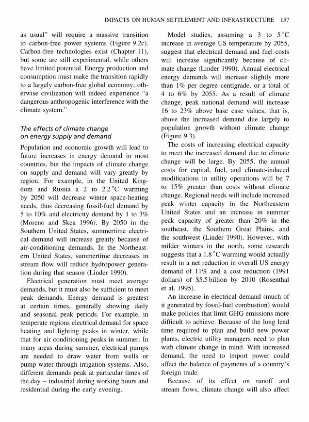
IMPACTS ON HUMAN SETTLEMENT AND INFRASTRUCTURE 157
as usual” will require a massive transitionto carbon-free power systems (Figure 9.2c).Carbon-free technologies exist (Chapter 11),but some are still experimental, while othershave limited potential. Energy production andconsumption must make the transition rapidlyto a largely carbon-free global economy; oth-erwise civilization will indeed experience “adangerous anthropogenic interference with theclimate system.”
The effects of climate changeon energy supply and demand
Population and economic growth will lead tofuture increases in energy demand in mostcountries, but the impacts of climate changeon supply and demand will vary greatly byregion. For example, in the United King-dom and Russia a 2 to 2.2 ◦C warmingby 2050 will decrease winter space-heatingneeds, thus decreasing fossil-fuel demand by5 to 10% and electricity demand by 1 to 3%(Moreno and Skea 1996). By 2050 in theSouthern United States, summertime electri-cal demand will increase greatly because ofair-conditioning demands. In the Northeast-ern United States, summertime decreases instream flow will reduce hydropower genera-tion during that season (Linder 1990).
Electrical generation must meet averagedemands, but it must also be sufficient to meetpeak demands. Energy demand is greatestat certain times, generally showing dailyand seasonal peak periods. For example, intemperate regions electrical demand for spaceheating and lighting peaks in winter, whilethat for air conditioning peaks in summer. Inmany areas during summer, electrical pumpsare needed to draw water from wells orpump water through irrigation systems. Also,different demands peak at particular times ofthe day – industrial during working hours andresidential during the early evening.
Model studies, assuming a 3 to 5 ◦Cincrease in average US temperature by 2055,suggest that electrical demand and fuel costswill increase significantly because of cli-mate change (Linder 1990). Annual electricalenergy demands will increase slightly morethan 1% per degree centigrade, or a total of4 to 6% by 2055. As a result of climatechange, peak national demand will increase16 to 23% above base case values, that is,above the increased demand due largely topopulation growth without climate change(Figure 9.3).
The costs of increasing electrical capacityto meet the increased demand due to climatechange will be large. By 2055, the annualcosts for capital, fuel, and climate-inducedmodifications in utility operations will be 7to 15% greater than costs without climatechange. Regional needs will include increasedpeak winter capacity in the NortheasternUnited States and an increase in summerpeak capacity of greater than 20% in thesoutheast, the Southern Great Plains, andthe southwest (Linder 1990). However, withmilder winters in the north, some researchsuggests that a 1.8 ◦C warming would actuallyresult in a net reduction in overall US energydemand of 11% and a cost reduction (1991dollars) of $5.5 billion by 2010 (Rosenthalet al. 1995).
An increase in electrical demand (much ofit generated by fossil-fuel combustion) wouldmake policies that limit GHG emissions moredifficult to achieve. Because of the long leadtime required to plan and build new powerplants, electric utility managers need to planwith climate change in mind. With increaseddemand, the need to import power couldaffect the balance of payments of a country’sforeign trade.
Because of its effect on runoff andstream flows, climate change will also affect
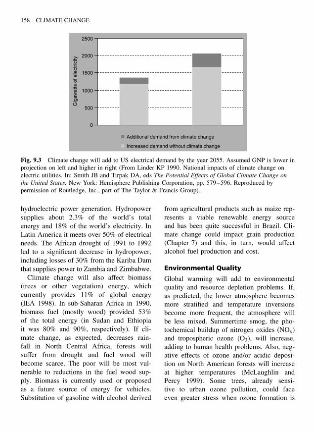
158 CLIMATE CHANGE
2500
2000
1500
1000
500
0
Additional demand from climate change
Gig
awat
ts o
f ele
ctric
ity
Increased demand without climate change
Fig. 9.3 Climate change will add to US electrical demand by the year 2055. Assumed GNP is lower inprojection on left and higher in right (From Linder KP 1990. National impacts of climate change onelectric utilities. In: Smith JB and Tirpak DA, eds The Potential Effects of Global Climate Change onthe United States. New York: Hemisphere Publishing Corporation, pp. 579–596. Reproduced bypermission of Routledge, Inc., part of The Taylor & Francis Group).
hydroelectric power generation. Hydropowersupplies about 2.3% of the world’s totalenergy and 18% of the world’s electricity. InLatin America it meets over 50% of electricalneeds. The African drought of 1991 to 1992led to a significant decrease in hydropower,including losses of 30% from the Kariba Damthat supplies power to Zambia and Zimbabwe.
Climate change will also affect biomass(trees or other vegetation) energy, whichcurrently provides 11% of global energy(IEA 1998). In sub-Saharan Africa in 1990,biomass fuel (mostly wood) provided 53%of the total energy (in Sudan and Ethiopiait was 80% and 90%, respectively). If cli-mate change, as expected, decreases rain-fall in North Central Africa, forests willsuffer from drought and fuel wood willbecome scarce. The poor will be most vul-nerable to reductions in the fuel wood sup-ply. Biomass is currently used or proposedas a future source of energy for vehicles.Substitution of gasoline with alcohol derived
from agricultural products such as maize rep-resents a viable renewable energy sourceand has been quite successful in Brazil. Cli-mate change could impact grain production(Chapter 7) and this, in turn, would affectalcohol fuel production and cost.
Environmental Quality
Global warming will add to environmentalquality and resource depletion problems. If,as predicted, the lower atmosphere becomesmore stratified and temperature inversionsbecome more frequent, the atmosphere willbe less mixed. Summertime smog, the pho-tochemical buildup of nitrogen oxides (NOx)and tropospheric ozone (O3), will increase,adding to human health problems. Also, neg-ative effects of ozone and/or acidic deposi-tion on North American forests will increaseat higher temperatures (McLaughlin andPercy 1999). Some trees, already sensi-tive to urban ozone pollution, could faceeven greater stress when ozone formation is
IMPACTS ON HUMAN SETTLEMENT AND INFRASTRUCTURE 159
enhanced by increased temperature and mois-ture from greenhouse warming (McLaughlinand Downing 1995). In regions where cli-mate change decreases precipitation, the inci-dence and intensity of brush and forest fireswill increase.
If, as models suggest, climate changeincreases the need for electricity, and addi-tional power capacity is required, then neg-ative environmental impacts could includethe following:
• decreased air quality (e.g. additional emis-sions of sulfur dioxide, nitrogen oxides, andother pollutants);
• increased land use for new power plantsites, fuel extraction and storage, and solidwaste disposal;
• increased water demand (e.g. for powerplant cooling and fuel processing);
• resource depletion of nonrenewable fuelssuch as natural gas.
On the other hand, reduction in fossil-fuel combustion, if achieved, would have theadded benefit of avoiding the costs of theseenvironmental impacts.
Extreme Climatic Events
Climate model projections for the twenty-firstcentury predict more extreme high temper-atures, fewer extreme low temperatures, areduced diurnal temperature range, increasedintensity of precipitation events, and midcon-tinental reductions in soil moisture. Changesin the frequency of occurrence and intensityof temperature and precipitation extremes canbe more important than changing long-termaverages. During the twentieth century, theincidence of climate extremes changed sig-nificantly (Easterling et al. 2000). Some areasexperienced fewer days of extreme cold or
precipitation, and some more days of extremeheat or precipitation, but these trends werenot universal. One widespread trend was anincrease in the average minimum temperatureand a decrease in the number of frost days.Also, one-day and multiday heavy precipi-tation events increased in many regions. InEurope, the warming trend between 1946 and1999 was generally accompanied by a slightincrease in wet extremes (ECAP 2002). In theUnited Kingdom, heavy precipitation eventsincreased in the winter and decreased in thesummer. Elsewhere, for example, the Sahelregion of Africa and China, the frequency andarea affected by drought increased. World-wide economic losses from storms increasedgreatly during the twentieth century. How-ever, these growing losses result more frompopulation growth and demographic shifts tomore storm-prone locations rather than fromgreater storm intensities.
Natural systems are vulnerable to increasesin climate extremes and the occurrence of cli-matic disturbances. The development or lifecycle of numerous organisms will be affectedby climate change (Box 6.2). For example,the maximum temperature experienced duringembryonic development determines the adultsex of many turtle species. In Britain andScandinavia, populations of birds, amphib-ians, and deer are affected by the periodicityand severity of the North Atlantic Oscillation(Box 8.2).
Some climate models suggest that a warmeratmosphere and ocean will add momen-tum to the sea–air exchange of energyand, thus, increase the frequency of tropi-cal cyclones, thunderstorms, tornadoes, hail-storms, droughts, and wildfires. For example,a doubling of CO2 may increase the inten-sity of tropical hurricanes and cyclones byas much as 40% (Emanuel 1987). In areaslike the Caribbean, the economic impacts
160 CLIMATE CHANGE
of such storms could increase significantly.These events could be made even more severein coastal areas by rising sea level.
Some models suggest an increase in theintensity of El Nino events, but othersdo not. Global models generally show lit-tle agreement when predicting changes inthe frequency or location of midlatitudestorms or tropical cyclones. However, morehigh-resolution regional models do suggestincreases in tropical cyclone intensities. Areview of numerous observed and predictedclimate extremes (Easterling et al. 2000) indi-cates the probability of changes during thiscentury, which include the following:
• very likely – higher maximum tempera-tures, more hot summer days, increase inthe heat index (combined temperature andhumidity), higher minimum temperatures,more heavy one-day and multiday precip-itation events, more heat waves, droughts,and reduced soil moisture at midlatitudes;
• likely – higher minimum temperatures andfewer frost days;
• possible – more intense tropical storms andEl Nino events.
Heavy precipitation events can cause flood-ing, erosion, and in mountainous regions,mudslides. Model predictions suggest that, formany temperate countries, heavy summer pre-cipitation events will increase by about 20%during this century – nearly four times theaverage overall precipitation increase (Gro-isman et al. 1999). Increased precipitationand runoff in some regions will lead to anincreased frequency and/or intensity of flood-ing with consequent economic costs. Forexample, model studies of New South Wales,Australia, predict that a CO2 doubling willresult in an increase in extremely heavy rain-fall events by a factor of 2 to 4. If the 1-in-400
year flood becomes the 1-in-100 year flood,combined residential and commercial dam-age in New South Wales would increase by$54 million to $313 million and the numberof residences flooded would double to quadru-ple (Smith and Hennessy 2002). In mountainregions people often live in settlements onsteep and potentially unstable hillsides. Land-slides from extreme rainfall events can havedevastating consequences.
Extreme climate events could significantlyincrease property insurance costs (Baker2002). Insurance companies are among theworld’s largest investors and have exten-sive real-state holdings. In 1992, total finan-cial losses from weather-related disasters costthe insurance industry a record $23 billion.With climate change, costs to insure againstextreme events and sea-level rise will surelyescalate. Some insurance companies, in res-ponse to climate-change forecasts, are dec-reasing their investments in coastal real estate,wildfire areas like Southern California, andflood-prone valleys. Eighty insurers fromaround the world signed the 2001 UnitedNations Environment Program, “Statement ofEnvironmental Commitment by the InsuranceIndustry” concerning global change and theenvironment. Skeptics argue that mitigativepolicy responses should wait until we aremore certain about the reality of climatechange. However, disaster insurers believethat these uncertainties make a compellingargument for taking climate change seriously.Without insurance, taxpayers and/or individ-uals will be called upon to pay the price ofclimate-induced disasters.
Human Settlements
Climate change will alter regional agriculturaland industrial potential and could triggerlarge-scale migrations and redistributions ofpeople. Such population displacements can

IMPACTS ON HUMAN SETTLEMENT AND INFRASTRUCTURE 161
result in serious socioeconomic disruptions,negative health impacts, and increased humansuffering (similar to the mass movement ofwar-related refugees). The lifestyle of mosthuman populations is adapted to a verynarrow range of climatic conditions. Humansettlements generally concentrate in areasof high industrial or agricultural potential,that is, areas with hospitable climates, nearcoastlines, in river and lake basins, or closeto major transportation routes.
Living patterns and technologies of partic-ular populations have evolved to cope withoccasional storms or disasters or slow nat-ural climate change, but not with rapid cli-mate change. Tens of thousands of yearsago, North Africa contained numerous largelakeside human settlements. As the climatechanged after the last glaciation, these pop-ulations gradually adapted by assuming anomadic way of life. However, a more rapid“desertification” of some semitropical regionsdue to climate change (Chapter 6) will notprovide time for such a gradual adaptation.
Desertification from tree removal, overgraz-ing, and other detrimental land-use practices isalready a global crisis. In sub-Saharan Africa,millions suffer from frequent drought-relatedcrop failures. Climate change will proba-bly accelerate this crisis. In other regions,as increased precipitation results in flood-ing, populations will need to abandon long-inhabited floodplains or construct expensivedam or levee systems.
Climate change, according to most sce-narios, will place added demands on urbaninfrastructures (Box 9.1). Urban populationsin much of the world are already experienc-ing explosive growth. Climate change couldaccelerate urbanization, as people migrateaway from low-lying coastal to interior areasor from drought-stricken farms to cities(IPCC 1990). Unabated, sea-level rise willhave devastating consequences for denselypopulated river delta areas in Egypt, India,Bangladesh, and elsewhere. Inhabitants willneed to migrate to mainland interior areas toescape flooding. For example, a 1-m sea-level
Box 9.1 Modeling infrastructure effects
The US EPA sponsors research on regional climate change in the United States, includingeffects on urban infrastructures. One project examines the future evolution of infrastructure inthe Boston Metropolitan Area. The project, Climate’s Long-Term Impacts on Metro Boston(CLIMB), attempts to document the present infrastructure and determine how climate changewill affect such things as flooding and drainage, water supply, water quality, built environment,energy, transportation, communication, and public health. A research team is formulating acomputer model to provide a tool for scenario analysis and policy development. The modelexamines effects over the period 2000 to 2100 and calculates three types of costs associatedwith climate-induced changes in infrastructure systems and services: loss of service cost, repairor replacement cost, and adaptation cost (CLIMB Project 2002). Preliminary results suggest anumber of significant effects of climate change on infrastructure.
Another study, the Metropolitan East Coast Assessment (MEC), covers areas of New York,Connecticut, and New Jersey with a regional population of 19.6 million. The MEC Projectfocuses on seven sectors: wetlands, transportation, infrastructure, water supply, public health,energy, and land-use decision-making (MEC 2002).
162 CLIMATE CHANGE
rise would seriously affect nearly a hundredmillion people along the coasts of Chinaalone (Han 1989). In some sea-level risescenarios, low-lying island nations virtuallycease to exist (Chapter 8). Migrating popu-lations would create infrastructure problemsfor regions suddenly faced with large numbersof “climate-change immigrants.” Additionalinfrastructure requirements would includemore housing, medical facilities, and otheressential urban services.
Infrastructure
Transportation
Climate change will impact the transportationsector in a number of ways. Industrial oragricultural relocations in response to climatechange will require additional investmentsin transportation – from new highways orrail links to new shipping ports. In manydeveloping countries the percentage of pavedroads is very low (the average for 15 differentAfrican countries is only 23%). In areas ofpredicted precipitation increases, landslidesand road erosion will raise maintenancecosts. Also, long-distance power and pipelineswill be threatened in areas of increasedprecipitation owing to slope instability andlandslides, and in arctic regions by warmingand melting of the supporting permafrost(Nelson et al. 2001).
Ship and barge transport are affected byclimate. Regional decreases in precipitationand runoff could reduce transport and nav-igation on rivers. For example, during theUS drought of 1988, low water in the Mis-sissippi River impeded barge traffic for sev-eral months. The reverse can also be true;increased flooding can lead to more siltationand impede river navigation. Marine ports inhigh-latitude areas, such as the oil fields ofPrudhoe Bay Alaska or Siberia, may bene-fit from a longer ice-free season following
global warming. In the US Great Lakes, mod-els suggest a longer ice-free shipping period.However, at the same time, lower precipita-tion and runoff will lead to lower lake lev-els and increased costs for dredging of GreatLakes ports (Smith 1990).
The growing number of automobiles in theworld, an expected increase from 400 millionto over 1 billion by the year 2030, will greatlyadd to GHG emissions, unless transportationalternatives are adopted soon. The average caremits 50 to 80 tons of CO2 over its full life,and the transportation infrastructure is respon-sible for a large percentage of CO2 emissions(35% in the United States and about 27%globally). The quantity of these emissionsper vehicle is a function of fuel efficiency.Automobile gasoline efficiency will need toincrease to 25 km L−1 (60 miles gallon−1) by2030 to maintain present fuel consumptionrates (Sierra Club 2002). Individual choicesand government policies regarding transporta-tion options have significant impacts on GHGemissions and resultant climate change. Forexample, a person traveling in a single occu-pant vehicle emits over five times the quantityof CO2 per distance traveled as a passengerusing a train or a bus (Figure 9.4).
Automobile commuting relates to urbanplanning and human settlement patterns. Inthe United States and Australia, decades oftown planning have led to suburban sprawland creation of the “Car City” where highintensities of auto commuting result in highlevels of GHG emissions. In contrast, citiesin Europe and Asia have generally remainedmore compact, and with greater public trans-port, more energy-efficient. Generally, com-muters tend to use automobiles less frequentlywhen there are more people and jobs per area(Figure 9.5). However, some city planners inthe United States and Australia are taking anew approach – designing urban centers that
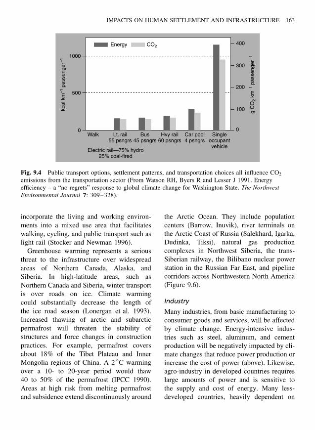
IMPACTS ON HUMAN SETTLEMENT AND INFRASTRUCTURE 163
1000
500
0
400
300
200
100
0Walk Lt. rail
55 psngrsBus
45 psngrsHvy rail
60 psngrs
kcal
km
−1 p
asse
nger
−1
g C
O2
km−1
pas
seng
er−1
Car pool4 psngrs
Singleoccupantvehicle
Electric rail—75% hydro25% coal-fired
Energy CO2
Fig. 9.4 Public transport options, settlement patterns, and transportation choices all influence CO2
emissions from the transportation sector (From Watson RH, Byers R and Lesser J 1991. Energyefficiency – a “no regrets” response to global climate change for Washington State. The NorthwestEnvironmental Journal 7: 309–328).
incorporate the living and working environ-ments into a mixed use area that facilitateswalking, cycling, and public transport such aslight rail (Stocker and Newman 1996).
Greenhouse warming represents a seriousthreat to the infrastructure over widespreadareas of Northern Canada, Alaska, andSiberia. In high-latitude areas, such asNorthern Canada and Siberia, winter transportis over roads on ice. Climate warmingcould substantially decrease the length ofthe ice road season (Lonergan et al. 1993).Increased thawing of arctic and subarcticpermafrost will threaten the stability ofstructures and force changes in constructionpractices. For example, permafrost coversabout 18% of the Tibet Plateau and InnerMongolia regions of China. A 2 ◦C warmingover a 10- to 20-year period would thaw40 to 50% of the permafrost (IPCC 1990).Areas at high risk from melting permafrostand subsidence extend discontinuously around
the Arctic Ocean. They include populationcenters (Barrow, Inuvik), river terminals onthe Arctic Coast of Russia (Salekhard, Igarka,Dudinka, Tiksi), natural gas productioncomplexes in Northwest Siberia, the trans-Siberian railway, the Bilibano nuclear powerstation in the Russian Far East, and pipelinecorridors across Northwestern North America(Figure 9.6).
Industry
Many industries, from basic manufacturing toconsumer goods and services, will be affectedby climate change. Energy-intensive indus-tries such as steel, aluminum, and cementproduction will be negatively impacted by cli-mate changes that reduce power production orincrease the cost of power (above). Likewise,agro-industry in developed countries requireslarge amounts of power and is sensitive tothe supply and cost of energy. Many less-developed countries, heavily dependent on
164 CLIMATE CHANGE
Fig. 9.5 Auto commuting and fuel consumption decreases with increasing urban population density(Reproduced from Stocker L and Newman P 1996. Urban design and transport options: strategies todecrease greenhouse gas emissions. In: Bouma WJ, Pearman GI and Manning MR, eds Greenhouse:Coping With Climate Change. Collingwood, VIC 3006, Australia: CSIRO Publishing, by permission ofCSIRO Publishing).
subsistence food and fiber production, are par-ticularly vulnerable to climate change. In con-trast, climate change may have little directeffect on food supplies in oil-rich countries ofthe Middle East, where domestic agriculturalproduction is small (Pilifosova 1998).
Industries, in some areas, will need to relo-cate to avoid flooding from sea-level rise ordrought-induced water shortages. In high lat-itudes, such as Canada and Siberia, climatewarming could lead to an increase in agri-culture, forestry, mining, industry, and human
Image Not Available
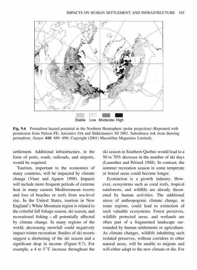
IMPACTS ON HUMAN SETTLEMENT AND INFRASTRUCTURE 165
Stable Low HighModerate
Fig. 9.6 Permafrost hazard potential in the Northern Hemisphere (polar projection) (Reprinted withpermission from Nelson FE, Anisimov OA and Shiklomanov NI 2001. Subsidence risk from thawingpermafrost. Nature 410: 889–890. Copyright (2001) Macmillan Magazines Limited).
settlement. Additional infrastructure, in theform of ports, roads, railroads, and airports,would be required.
Tourism, important to the economies ofmany countries, will be impacted by climatechange (Viner and Agnew 1999). Impactswill include more frequent periods of extremeheat in many eastern Mediterranean resortsand loss of beaches or reefs from sea-levelrise. In the United States, tourism in NewEngland’s White Mountain region is related tothe colorful fall foliage season, ski season, andrecreational fishing – all potentially affectedby climate change. In many regions of theworld, decreasing snowfall could negativelyimpact winter recreation. Studies of ski resortssuggest a shortening of the ski season and asignificant drop in income (Figure 9.7). Forexample, a 4 to 5 ◦C increase throughout the
ski season in Southern Quebec would lead to a50 to 70% decrease in the number of ski days(Lamother and Periard 1988). In contrast, thesummer recreation season in some temperateor boreal areas could become longer.
Ecotourism is a growth industry. How-ever, ecosystems such as coral reefs, tropicalrainforests, and wildlife are already threat-ened by human activities. The additionalstress of anthropogenic climate change, insome regions, could lead to extinction ofsuch valuable ecosystems. Forest preserves,wildlife protected areas, and wetlands areoften part of a fragmented landscape sur-rounded by human settlements or agriculture.As climate changes, wildlife inhabiting suchisolated preserves, without corridors to othernatural areas, will be unable to migrate andwill either adapt to the new climate or die. For
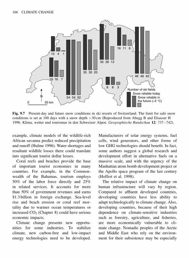
166 CLIMATE CHANGE
0 50 km
N
15
19 16 7
4 1
35 30 20
8 8 3
35 26 13
46 46 42
16 11 6
54 54 52
Number of ski fieldsSnow reliable today
Snow reliable inthe future (+2 °C)
Fig. 9.7 Present-day and future snow conditions in ski resorts of Switzerland. The limit for safe snowconditions is set at 100 days with a snow depth >30 cm (Reproduced from Abegg B and Elsasser H1996. Klima, wetter und tourismus in den Schweizer Alpen. Geographische Rundschau 12: 737–742).
example, climate models of the wildlife-richAfrican savanna predict reduced precipitationand runoff (Hulme 1996). Water shortages andresultant wildlife losses there could translateinto significant tourist dollar losses.
Coral reefs and beaches provide the baseof important tourist economies in manycountries. For example, in the Common-wealth of the Bahamas, tourism employs50% of the labor force directly and 25%in related services. It accounts for morethan 50% of government revenues and earns$1.3 billion in foreign exchange. Sea-levelrise and beach erosion or coral reef mor-tality due to warmer ocean temperatures orincreased CO2 (Chapter 8) could have seriouseconomic impacts.
Climate change presents new opportu-nities for some industries. To stabilizeclimate, new carbon-free and low-impactenergy technologies need to be developed.
Manufacturers of solar energy systems, fuelcells, wind generators, and other forms oflow GHG technologies should benefit. In fact,some authors suggest a global research anddevelopment effort in alternative fuels on amassive scale, and with the urgency of theManhattan atom bomb development project orthe Apollo space program of the last century(Hoffert et al. 1998).
The relative impact of climate change onhuman infrastructure will vary by region.Compared to affluent developed countries,developing countries have less ability toadapt technologically to climate change. Also,developing countries, because of their highdependence on climate-sensitive industriessuch as forestry, agriculture, and fisheries,are more economically vulnerable to cli-mate change. Nomadic peoples of the Arcticand Middle East who rely on the environ-ment for their subsistence may be especially
IMPACTS ON HUMAN SETTLEMENT AND INFRASTRUCTURE 167
vulnerable. In the United States, while Cleve-land, Ohio, may expect to save $4.5 milliona year in reduced snow and ice removalcosts, Miami, Florida, may need to invest$600 million during this century to deal withproblems of sea-level rise (Miller 1989).Venice, Italy, is again reviewing a pro-posed $2 billion floodgate system, as well asother measures, to factor in sea-level rise(Chapter 8). Also, urban areas, because ofpavement cover, buildings, and air pollution,suffer from the “urban heat island effect.”Cities such as Shanghai, China, can experi-ence temperatures of 5 ◦C or more greater thanthe surrounding countryside. Climate changemay enhance this effect and add to poten-tial health problems related to heat stress(Chapter 10).
Summary
Climate will probably lead to shifts inregional patterns of energy use. These includesome reduction in space-heating requirementsin temperate regions and increased energyrequirements for air conditioning and irri-gation in less temperate regions. Additionalenergy consumption could further compro-mise environmental quality. To avoid a dan-gerous anthropogenic interference with theclimate system, a massive shift to carbon-freepower systems must be accomplished.
Human populations are heavily concen-trated in urban centers and more than 80% livewithin 300 km of coastlines. Models predictincreases in extreme climatic events, such aswindstorms, heavy precipitation and flooding,heat waves, and droughts. This could resultin even greater impacts on human settlementpatterns and infrastructure with serious eco-nomic consequences. Settlement patterns willprobably shift in some regions in responseto decreasing rainfall (desertification) and in
other regions in response to increasing rain-fall (flooding). Millions living near low-lyingcoastal areas will be displaced if the projected100-year rise in global sea level is not averted.
Transportation depends on highways, brid-ges, and rivers. Shifting settlement patterns,more frequent extreme weather events, ormelting permafrost could challenge transportsystems. Industries, especially those heav-ily dependent on resources or the environ-ment, such as agriculture, forestry, fisheries,and tourism (often the case in developingcountries), are especially vulnerable to cli-mate change. Many industries, including elec-tric utilities, insurance, resource harvesting(forestry and fisheries), and tourism are ana-lyzing and planning their possible options foradapting to or reducing their vulnerability toclimate change.
References
Abegg B and Elsasser H 1996 Klima, wetter undtourismus in den Schweizer Alpen. GeographischeRundschau 12: 737–742.
Baker JD 2002 Climate change and the re-insuranceindustry. Presentation to the Reinsurance Associ-ation of America, May 24, 2000. Available from:http://www.noaa.gov/baker/reinsure/speech1.html.
CLIMB Project 2002 Available from: http://www.tufts.edu/tie/climb/.
Easterling DR, Meehl GA, Parmesan C, ChangnonSA, Karl TR and Mearns LO 2000 Climateextremes: observations, modeling, and impacts.Science 289: 2068–2074.
Emanuel KA 1987 The dependence of hurricaneintensity on climate. Nature 326: 483–485.
ECAP 2002 Available from: http://www.knmi.nl/voorl/.
Gore A 1993 Chapter 3, Climate and civilization,Earth in the Balance: Ecology and the HumanSpirit . New York: Plume Publishing, pp. 56–80.
Groisman PY, Karl TR, Easterling DR, Knight RW,Jamason PF, Hennessay KJ, et al. 1999 Changesin the probability of heavy precipitation: importantindicators of climatic change. Climatic Change 42:243–283.
168 CLIMATE CHANGE
Han M 1989 Global warming induced sea level risein China: response and strategies. Presentationto World Conference on Preparing for ClimateChange December 19, Cairo, Egypt.
Hoffert MI, Caldeira K, Jain AK, Haites EF, DannyHarvey LD, Potter SD, et al. 1998 Energy impli-cations of future stabilization of atmospheric CO2
content. Nature 395: 881–884.Hulme M 1996 Chapter 5, Climatic change within
the period of meteorological records. In: AdamsWM, Goudie AS and Orme AR, eds The PhysicalGeography of Africa . Oxford: Oxford UniversityPress, pp. 88–102.
IEA 1998 Biomass Energy: Data, Analysis, andTrends . Paris: International Energy Agency, p. 339,http://www.iea.org/index.html .
IPCC 1990 Potential impacts of climate change:human settlement; energy, transport and industrialsectors; human health; air quality, and changesin ultraviolet-B radiation . Intergovernmental Panelon Climate Change, Working Group II (A. Izrael,Chair). Geneva WMO/UNEP, p. 34.
Lamother AM and Periard G 1988 Implications ofclimate change for downhill skiing in Quebec.Climate Change Digest: CCD 88-03. Downsview .Ontario: Environment Canada, p. 12.
Linder KP 1990 National impacts of climate changeon electric utilities. In: Smith JB and Tirpak DA,eds The Potential Effects of Global Climate Changeon the United States . New York: HemispherePublishing Corporation, pp. 579–596.
Lonergan S, DiFrancesco R and Woo M 1993Climate change and transportation in NorthernCanada: an integrated impact assessment. ClimaticChange 24(4): 331–351.
McLaughlin SB and Downing DJ 1995 Interactiveeffects of ambient ozone and climate measuredon growth of mature forest trees. Nature 374:252–254.
McLaughlin S and Percy K 1999 Forest health inNorth America: some perspectives on actual andpotential roles of climate and air pollution. Waterand Soil Pollution 116(1–2): 151–197.
MEC 2002 Metropolitan East Coast Assessment.New York: Center for International Earth ScienceInformation Network (CIESIN) Columbia Uni-versity, Available from: http://metroeast climate.ciesin.columbia.edu/ .
Miller TR 1989 Impacts of global climate changeon metropolitan infrastructure. In: Topping Jr JC,ed. Coping With Climate Change. Proceedings of
the Second North American Conference on Prepar-ing for Climate Change. Washington, DC: ClimateInstitute, 6–8 December, pp. 366–376.
Moreno RA and Skea J 1996 Industry, Energy,and Transportation: Impacts and Adaptation,Chapter 11. In: Houghton JT, Meira LG, Callan-der BA, Harris N, Kattenberg A, Maskell K, edsClimate Change 1995: The Science of ClimateChange. Intergovernmental Panel on ClimateChange. Cambridge: Cambridge University Press,pp. 365–398.
Nelson FE, Anisimov OA and Shiklomanov NI 2001Subsidence risk from thawing permafrost. Nature410: 889,890.
Pearson PJG and Fouquet R 1996 Energy efficiency,economic efficiency and future CO2 emissionsfrom the developing world. The Energy Journal17(4): 135–159.
Pilifosova O 1998 Middle East and Arid Asia.Chapter 7. In: Watson RT, Zinyowera MC andMoss RH, eds The Regional Impacts of Cli-mate Change: An Assessment of Vulnerability.Intergovernmental Panel on Climate Change.Cambridge: Cambridge University Press, pp. 231–252.
Rosenthal DH, Gruenspecht HK and Moran E 1995Effects of global warming on energy use for spaceheating and cooling in the United States. EnergyJournal 16(2): 77–96.
Sierra Club 2002 Available from: http://www.sierraclub.org/global-warming.
Smith DI and Hennessy K 2002 Climate change,flooding and urban infrastructure. AustralianNational University and CSIRO AtmosphericResearch. Available from: http://dar.csiro.au/res/cm/c7.htm.
Smith J 1990 Great lakes. In: Smith JB and Tir-pak DA, eds The Potential Effects of Global Cli-mate Change on the United States . US EPA, Wash-ington, DC: Hemisphere Publishing Corporation,pp. 121–182.
Stocker L and Newman P 1996 Urban design andtransport options: strategies to decrease greenhousegas emissions. In: Bouma WJ, Pearman GI andManning MR, eds Greenhouse: Coping With Cli-mate Change. Collingwood, VIC 3006, Australia:CSIRO Publishing, pp. 520–537.
UNFCCC 2002 Available from: http://unfccc.int/.

IMPACTS ON HUMAN SETTLEMENT AND INFRASTRUCTURE 169
Viner D and Agnew M 1999 Climate change and itsimpact on tourism. Report prepared for the WorldWildlife Fund. UK: Climate Change ResearchUnit, University of East Anglia, p. 50.
Watson RH, Byers R and Lesser J 1991 Energy effi-ciency – a “no regrets” response to global climatechange for Washington State. The Northwest Envi-ronmental Journal 7: 309–328.

This Page Intentionally Left Blank
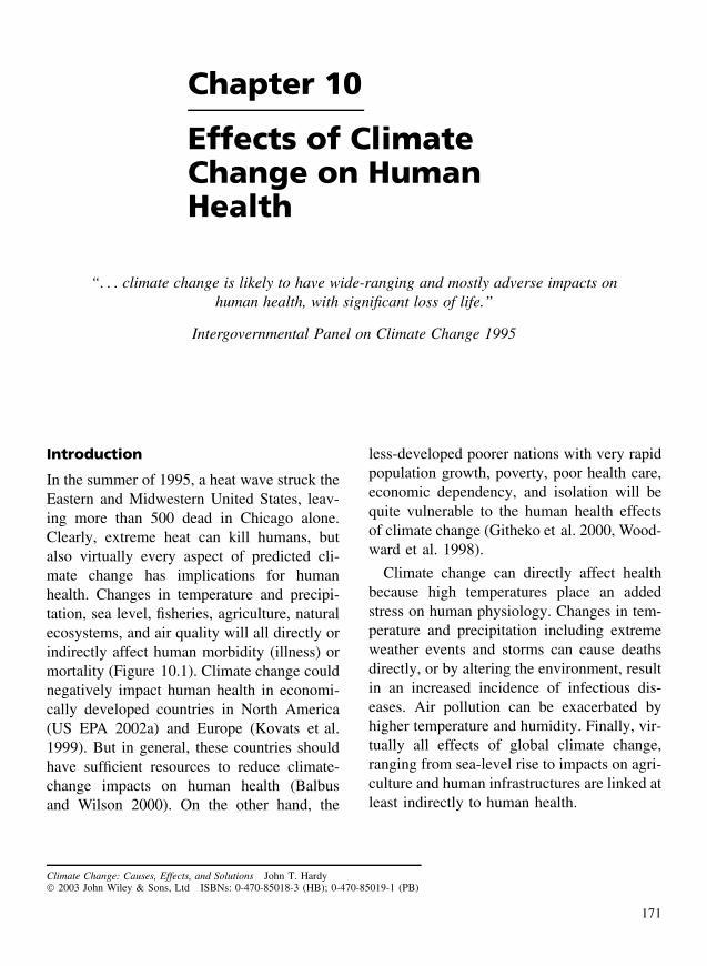
Chapter 10
Effects of ClimateChange on HumanHealth
“. . . climate change is likely to have wide-ranging and mostly adverse impacts onhuman health, with significant loss of life.”
Intergovernmental Panel on Climate Change 1995
Introduction
In the summer of 1995, a heat wave struck theEastern and Midwestern United States, leav-ing more than 500 dead in Chicago alone.Clearly, extreme heat can kill humans, butalso virtually every aspect of predicted cli-mate change has implications for humanhealth. Changes in temperature and precipi-tation, sea level, fisheries, agriculture, naturalecosystems, and air quality will all directly orindirectly affect human morbidity (illness) ormortality (Figure 10.1). Climate change couldnegatively impact human health in economi-cally developed countries in North America(US EPA 2002a) and Europe (Kovats et al.1999). But in general, these countries shouldhave sufficient resources to reduce climate-change impacts on human health (Balbusand Wilson 2000). On the other hand, the
less-developed poorer nations with very rapidpopulation growth, poverty, poor health care,economic dependency, and isolation will bequite vulnerable to the human health effectsof climate change (Githeko et al. 2000, Wood-ward et al. 1998).
Climate change can directly affect healthbecause high temperatures place an addedstress on human physiology. Changes in tem-perature and precipitation including extremeweather events and storms can cause deathsdirectly, or by altering the environment, resultin an increased incidence of infectious dis-eases. Air pollution can be exacerbated byhigher temperature and humidity. Finally, vir-tually all effects of global climate change,ranging from sea-level rise to impacts on agri-culture and human infrastructures are linked atleast indirectly to human health.
Climate Change: Causes, Effects, and Solutions John T. Hardy 2003 John Wiley & Sons, Ltd ISBNs: 0-470-85018-3 (HB); 0-470-85019-1 (PB)
171
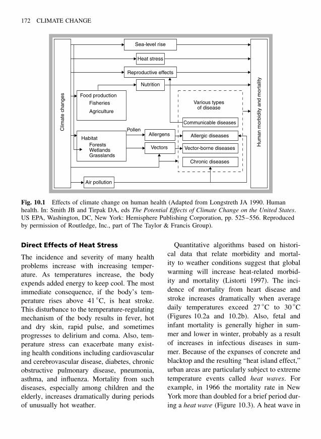
172 CLIMATE CHANGE
Sea-level rise
Heat stress
Nutrition
Air pollution
Reproductive effects
Food production
Fisheries
Agriculture
ForestsWetlandsGrasslands
Habitat
PollenAllergens
Vectors
Various typesof disease
Communicable diseases
Allergic diseases
Vector-borne diseases
Chronic diseases
Clim
ate
chan
ges
Hum
an m
orbi
dity
and
mor
talit
y
Fig. 10.1 Effects of climate change on human health (Adapted from Longstreth JA 1990. Humanhealth. In: Smith JB and Tirpak DA, eds The Potential Effects of Climate Change on the United States.US EPA, Washington, DC, New York: Hemisphere Publishing Corporation, pp. 525–556. Reproducedby permission of Routledge, Inc., part of The Taylor & Francis Group).
Direct Effects of Heat Stress
The incidence and severity of many healthproblems increase with increasing temper-ature. As temperatures increase, the bodyexpends added energy to keep cool. The mostimmediate consequence, if the body’s tem-perature rises above 41 ◦C, is heat stroke.This disturbance to the temperature-regulatingmechanism of the body results in fever, hotand dry skin, rapid pulse, and sometimesprogresses to delirium and coma. Also, tem-perature stress can exacerbate many exist-ing health conditions including cardiovascularand cerebrovascular disease, diabetes, chronicobstructive pulmonary disease, pneumonia,asthma, and influenza. Mortality from suchdiseases, especially among children and theelderly, increases dramatically during periodsof unusually hot weather.
Quantitative algorithms based on histori-cal data that relate morbidity and mortal-ity to weather conditions suggest that globalwarming will increase heat-related morbid-ity and mortality (Listorti 1997). The inci-dence of mortality from heart disease andstroke increases dramatically when averagedaily temperatures exceed 27 ◦C to 30 ◦C(Figures 10.2a and 10.2b). Also, fetal andinfant mortality is generally higher in sum-mer and lower in winter, probably as a resultof increases in infectious diseases in sum-mer. Because of the expanses of concrete andblacktop and the resulting “heat island effect,”urban areas are particularly subject to extremetemperature events called heat waves. Forexample, in 1966 the mortality rate in NewYork more than doubled for a brief period dur-ing a heat wave (Figure 10.3). A heat wave in

EFFECTS OF CLIMATE CHANGE ON HUMAN HEALTH 173
Fig. 10.2 Relationship of temperature and mortality from (a) heart disease and (b) stroke (From RogotE and Padgett SJ 1976. Associations of coronary and stroke mortality with temperature and snowfall inselected areas of the United States 1962–1966. American Journal of Epidemiology 103: 565–575, bypermission of Oxford University Press).
Image Not Available
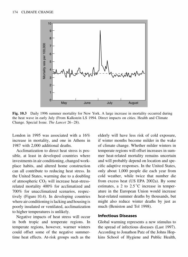
174 CLIMATE CHANGE
May June July August
10
9
8
7
6
5
4
3
2
1
0
Mor
talit
y ra
te p
er 1
00,0
00
Fig. 10.3 Daily 1996 summer mortality for New York. A large increase in mortality occurred duringthe heat wave in early July (From Kalkstein LS 1994. Direct impacts on cities. Health and ClimateChange. Special Issue. The Lancet 26–28).
London in 1995 was associated with a 16%increase in mortality, and one in Athens in1987 with 2,000 additional deaths.
Acclimatization to direct heat stress is pos-sible, at least in developed countries whereinvestments in air conditioning, changed work-place habits, and altered home constructioncan all contribute to reducing heat stress. Inthe United States, warming due to a doublingof atmospheric CO2 will increase heat-stress-related mortality 400% for acclimatized and700% for unacclimatized scenarios, respec-tively (Figure 10.4). In developing countrieswhere air conditioning is lacking and housing ispoorly insulated or ventilated, acclimatizationto higher temperatures is unlikely.
Negative impacts of heat stress will occurin both tropic and temperate regions. Intemperate regions, however, warmer winterscould offset some of the negative summer-time heat effects. At-risk groups such as the
elderly will have less risk of cold exposure,if winter months become milder in the wakeof climate change. Whether milder winters intemperate regions will offset increases in sum-mer heat-related mortality remains uncertainand will probably depend on location and spe-cific adaptive responses. In the United States,only about 1,000 people die each year fromcold weather, while twice that number diefrom excess heat (US EPA 2002a). By someestimates, a 2 to 2.5 ◦C increase in temper-ature in the European Union would increaseheat-related summer deaths by thousands, butmight also reduce winter deaths by just asmuch (Beniston and Tol 1998).
Infectious Diseases
Global warming represents a new stimulus tothe spread of infectious diseases (Last 1997).According to Jonathon Patz of the Johns Hop-kins School of Hygiene and Public Health,
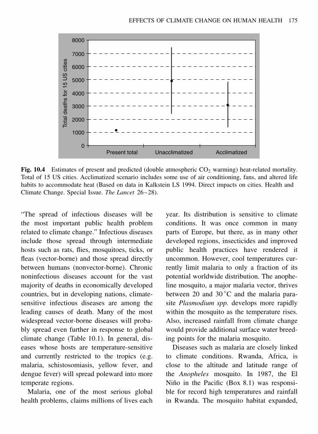
EFFECTS OF CLIMATE CHANGE ON HUMAN HEALTH 175
8000
7000
6000
5000
4000
3000
2000
1000
0Present total Unacclimatized
Tota
l dea
ths
for
15 U
S c
ities
Acclimatized
Fig. 10.4 Estimates of present and predicted (double atmospheric CO2 warming) heat-related mortality.Total of 15 US cities. Acclimatized scenario includes some use of air conditioning, fans, and altered lifehabits to accommodate heat (Based on data in Kalkstein LS 1994. Direct impacts on cities. Health andClimate Change. Special Issue. The Lancet 26–28).
“The spread of infectious diseases will bethe most important public health problemrelated to climate change.” Infectious diseasesinclude those spread through intermediatehosts such as rats, flies, mosquitoes, ticks, orfleas (vector-borne) and those spread directlybetween humans (nonvector-borne). Chronicnoninfectious diseases account for the vastmajority of deaths in economically developedcountries, but in developing nations, climate-sensitive infectious diseases are among theleading causes of death. Many of the mostwidespread vector-borne diseases will proba-bly spread even further in response to globalclimate change (Table 10.1). In general, dis-eases whose hosts are temperature-sensitiveand currently restricted to the tropics (e.g.malaria, schistosomiasis, yellow fever, anddengue fever) will spread poleward into moretemperate regions.
Malaria, one of the most serious globalhealth problems, claims millions of lives each
year. Its distribution is sensitive to climateconditions. It was once common in manyparts of Europe, but there, as in many otherdeveloped regions, insecticides and improvedpublic health practices have rendered ituncommon. However, cool temperatures cur-rently limit malaria to only a fraction of itspotential worldwide distribution. The anophe-line mosquito, a major malaria vector, thrivesbetween 20 and 30 ◦C and the malaria para-site Plasmodium spp. develops more rapidlywithin the mosquito as the temperature rises.Also, increased rainfall from climate changewould provide additional surface water breed-ing points for the malaria mosquito.
Diseases such as malaria are closely linkedto climate conditions. Rwanda, Africa, isclose to the altitude and latitude range ofthe Anopheles mosquito. In 1987, the ElNino in the Pacific (Box 8.1) was responsi-ble for record high temperatures and rainfallin Rwanda. The mosquito habitat expanded,
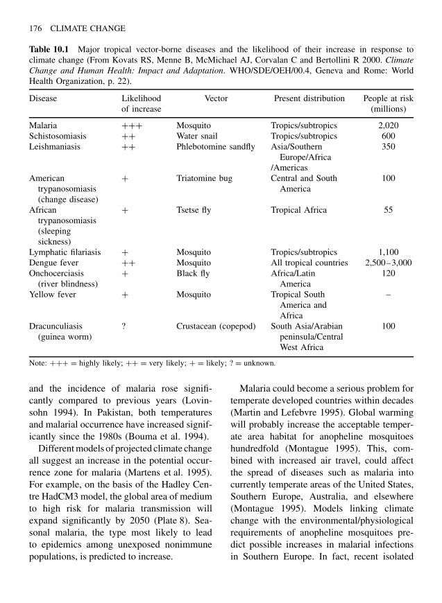
176 CLIMATE CHANGE
Table 10.1 Major tropical vector-borne diseases and the likelihood of their increase in response toclimate change (From Kovats RS, Menne B, McMichael AJ, Corvalan C and Bertollini R 2000. ClimateChange and Human Health: Impact and Adaptation. WHO/SDE/OEH/00.4, Geneva and Rome: WorldHealth Organization, p. 22).
Disease Likelihoodof increase
Vector Present distribution People at risk(millions)
Malaria +++ Mosquito Tropics/subtropics 2,020Schistosomiasis ++ Water snail Tropics/subtropics 600Leishmaniasis ++ Phlebotomine sandfly Asia/Southern
Europe/Africa/Americas
350
Americantrypanosomiasis(change disease)
+ Triatomine bug Central and SouthAmerica
100
Africantrypanosomiasis(sleepingsickness)
+ Tsetse fly Tropical Africa 55
Lymphatic filariasis + Mosquito Tropics/subtropics 1,100Dengue fever ++ Mosquito All tropical countries 2,500–3,000Onchocerciasis
(river blindness)+ Black fly Africa/Latin
America120
Yellow fever + Mosquito Tropical SouthAmerica andAfrica
–
Dracunculiasis(guinea worm)
? Crustacean (copepod) South Asia/Arabianpeninsula/CentralWest Africa
100
Note: +++ = highly likely; ++ = very likely; + = likely; ? = unknown.
and the incidence of malaria rose signifi-cantly compared to previous years (Lovin-sohn 1994). In Pakistan, both temperaturesand malarial occurrence have increased signif-icantly since the 1980s (Bouma et al. 1994).
Different models of projected climate changeall suggest an increase in the potential occur-rence zone for malaria (Martens et al. 1995).For example, on the basis of the Hadley Cen-tre HadCM3 model, the global area of mediumto high risk for malaria transmission willexpand significantly by 2050 (Plate 8). Sea-sonal malaria, the type most likely to leadto epidemics among unexposed nonimmunepopulations, is predicted to increase.
Malaria could become a serious problem fortemperate developed countries within decades(Martin and Lefebvre 1995). Global warmingwill probably increase the acceptable temper-ate area habitat for anopheline mosquitoeshundredfold (Montague 1995). This, com-bined with increased air travel, could affectthe spread of diseases such as malaria intocurrently temperate areas of the United States,Southern Europe, Australia, and elsewhere(Montague 1995). Models linking climatechange with the environmental/physiologicalrequirements of anopheline mosquitoes pre-dict possible increases in malarial infectionsin Southern Europe. In fact, recent isolated
EFFECTS OF CLIMATE CHANGE ON HUMAN HEALTH 177
cases of malaria in Italy and the EasternUnited States are consistent with this hypoth-esis (Martens 1999).
In many areas, malaria is limited to warmerlowland elevations and excluded by the coolertemperatures of highland elevations. In the-ory, a small increase in temperature couldopen highland areas of many countries tothe malaria parasite. However, no correlationseems to exist between recent climate changeand malaria resurgence at high-altitude sitesin East Africa (Hay et al. 2002).
Climate-change models (HadCM3) pre-dict an additional 300 million cases ofP. falciparum and 150 million cases ofP. vivax types of malaria worldwide by 2080(Martens et al. 1999). The greatest increasein potential transmission for malaria will bein Central Asia, North America, and Europe,where the vector mosquitoes are present,but where current climates are too cold fortransmission. In South America, the numberof persons at risk of infection from year-round malaria transmission will double from25 million to 50 million between 2020 and2080 (Martens et al. 1999).
The range of dengue fever will probablyexpand in response to climate change. Denguefever, spread by the mosquito Aedes aegypti,is the most important vector-borne viral dis-ease in the world with up to 100 millioncases per year (Kovats et al. 1999). Highertemperatures increase the efficiency of Aedesmosquitoes in transmitting the dengue virus(Watts et al. 1987). Model predictions sug-gest that in response to climate change, themosquito will expand its latitudinal distribu-tion during the warmer months (Hopp andFoley 2001). Freezing temperatures kill themosquito eggs, but as the minimum temper-ature – for overwintering its eggs and lar-vae – moves poleward with climate change,much of Central and Southern Europe (Ward
and Burgess 1993) as well as the United Statescould be at risk. Climate-change models pre-dict increases in rainfall and temperature forparts of Australia that could increase the threatof several mosquito-borne viruses, includingdengue fever, by extending the season of themosquito vectors (Russell 1998).
Increasing global travel and trade has ledto the spread of disease vectors to new areas.The major vector of dengue fever, Aedesalbopictus, was introduced into the UnitedStates from East Asia in shipments of usedcar tires and has now spread through much ofNorth America. In Italy, the same mosquitohas spread to 22 northern provinces sinceits appearance in about 1992. West Nileviral encephalitis, another sometimes deadlydisease carried by Culex mosquitoes, andhosted by birds, broke out in France inthe 1960s. Perhaps in response to a verywarm summer along the east coast of NorthAmerica, it appeared in New York in 1999.It is now spreading across the United States.Its link to climate change remains unclear, butcertainly warmer temperatures could enhanceits spread.
Schistosomiasis (Bilharzia), another vector-borne disease, infects perhaps as many as200 million people worldwide. It is a water-borne parasitic worm whose eggs enter watersupplies by way of human feces or urine. Theparasitic worm and its intermediate host, asnail, thrive in warm water. In countries likeEgypt, the snail population declines duringthe cooler months, but climate warming willextend the season and incidence of infection.
Hantavirus is spread though the saliva andfeces of deer mice. In the SouthwesternUnited States in 1993, heavy rains followinga six-year drought provided an abundant foodsupply of pine nuts and ideal conditions fora rodent vector population explosion. Thiswas followed by an outbreak of the deadly
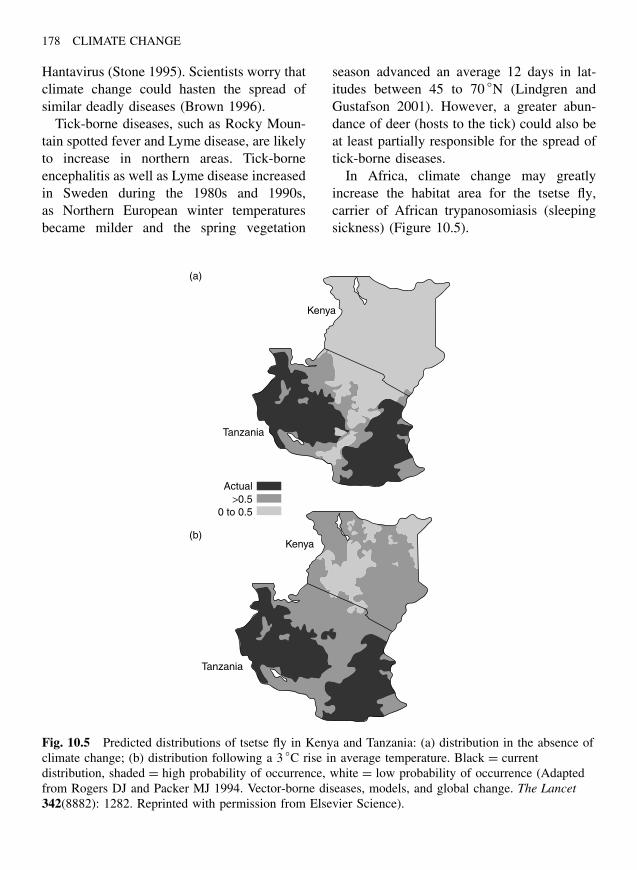
178 CLIMATE CHANGE
Hantavirus (Stone 1995). Scientists worry thatclimate change could hasten the spread ofsimilar deadly diseases (Brown 1996).
Tick-borne diseases, such as Rocky Moun-tain spotted fever and Lyme disease, are likelyto increase in northern areas. Tick-borneencephalitis as well as Lyme disease increasedin Sweden during the 1980s and 1990s,as Northern European winter temperaturesbecame milder and the spring vegetation
season advanced an average 12 days in lat-itudes between 45 to 70 ◦N (Lindgren andGustafson 2001). However, a greater abun-dance of deer (hosts to the tick) could also beat least partially responsible for the spread oftick-borne diseases.
In Africa, climate change may greatlyincrease the habitat area for the tsetse fly,carrier of African trypanosomiasis (sleepingsickness) (Figure 10.5).
Kenya
Kenya
Tanzania
Tanzania
Actual>0.5
0 to 0.5
(a)
(b)
Fig. 10.5 Predicted distributions of tsetse fly in Kenya and Tanzania: (a) distribution in the absence ofclimate change; (b) distribution following a 3 ◦C rise in average temperature. Black = currentdistribution, shaded = high probability of occurrence, white = low probability of occurrence (Adaptedfrom Rogers DJ and Packer MJ 1994. Vector-borne diseases, models, and global change. The Lancet342(8882): 1282. Reprinted with permission from Elsevier Science).
EFFECTS OF CLIMATE CHANGE ON HUMAN HEALTH 179
Some nonvector-borne diseases could alsoincrease in response to climate change. Pop-ulation explosions of certain toxin-containingmarine algae, “toxic algal blooms,” are increas-ing globally. In fact, the world seems to beexperiencing a “global epidemic” of harmfulcoastal algal blooms (Epstein et al. 1994, VanDolah 2000). Humans are poisoned from eatingalgal-contaminated shellfish or from breath-ing marine aerosols containing such algae.Cholera (Vibrio cholerae) is a waterborne dis-ease, which in its dormant state is quite salt-tolerant. Some evidence suggests that choleraoutbreaks in several coastal areas may be linkedto warm-water events and associated planktonblooms that concentrate the pathogen (Colwelland Huq 1994). In 1992, a new strain of choleraemerged in coastal areas of India and beganspreading in Asia. Finally, food-related infec-tions, such as food poisoning from salmonel-losis, thrive at warmer temperatures and couldbecome more common (UKDH 2001).
Air Quality
Air pollution, an exacerbating factor forpulmonary health conditions such as asthma
and cardiorespiratory disorders, will proba-bly increase as a result of climate change.Increased energy demand (Chapter 9) will addto fossil-fuel combustion. This will increaseemissions of particulates (a cause of respira-tory problems), toxic aromatic hydrocarbons(carcinogens), and sulfur dioxide (acid rain).Air quality is a function not only of pollu-tant emissions but also of atmospheric circu-lation and mixing. Thus, if climate changecauses increased atmospheric stratification,pollutants will tend to accumulate near theEarth’s surface.
Climate change will increase ozone pollu-tion. Increased temperature and water vapor,along with increased ultraviolet-b (UV-b)radiation from stratospheric ozone deple-tion, will accelerate the chemical transfor-mations that form tropospheric ozone (smog)(Box 10.1). Ozone and the photochemicalproducts formed, such as peroxides, arelung irritants. Global climate models predictabout a 20-ppbv (parts per billion by vol-ume) or 40% increase in the atmosphericconcentration of ozone in midsummer in Cen-tral England between 1990 and 2100 (UKDH
Box 10.1 Ozone and photochemical smog formation (Adapted from US EPA 2002b.Air Quality Planning and Standards. Unites States Environmental ProtectionAgency. Available from: http://www.epa.gov/oar/oaqps)
Tropospheric Ozone – Tropospheric ozone, “bad ozone,” is an air pollutant. It shouldnot be confused with “good ozone,” present in the stratosphere, which protects life fromthe damaging effects of ultraviolet radiation (Box 1.4). Motor vehicle exhaust, industrialemissions, gasoline vapors, and chemical solvents release nitrogen oxides (NOx) and volatileorganic compounds (VOC). Strong sunlight and hot weather promote the transformation ofthese chemicals and the formation of tropospheric ozone. Many urban areas tend to have highlevels of “bad” ozone, but other areas are also subject to high ozone levels as winds carryNOx emissions hundreds of miles away from their original sources. Ozone concentrationscan vary from year to year. Changing weather patterns (especially the number of hot, sunnydays), periods of air stagnation, and other factors that contribute to ozone formation makelong-term predictions difficult.
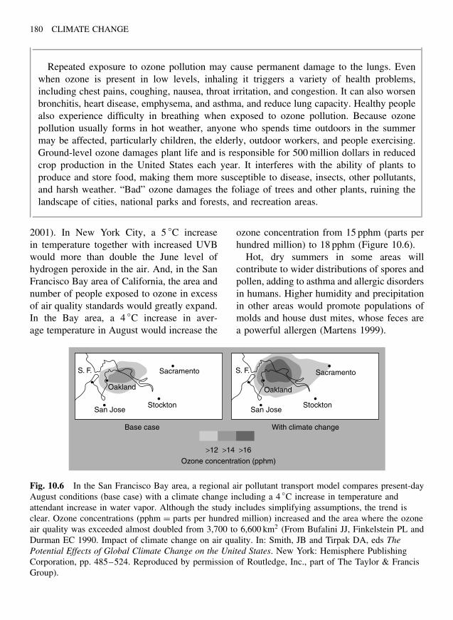
180 CLIMATE CHANGE
Repeated exposure to ozone pollution may cause permanent damage to the lungs. Evenwhen ozone is present in low levels, inhaling it triggers a variety of health problems,including chest pains, coughing, nausea, throat irritation, and congestion. It can also worsenbronchitis, heart disease, emphysema, and asthma, and reduce lung capacity. Healthy peoplealso experience difficulty in breathing when exposed to ozone pollution. Because ozonepollution usually forms in hot weather, anyone who spends time outdoors in the summermay be affected, particularly children, the elderly, outdoor workers, and people exercising.Ground-level ozone damages plant life and is responsible for 500 million dollars in reducedcrop production in the United States each year. It interferes with the ability of plants toproduce and store food, making them more susceptible to disease, insects, other pollutants,and harsh weather. “Bad” ozone damages the foliage of trees and other plants, ruining thelandscape of cities, national parks and forests, and recreation areas.
2001). In New York City, a 5 ◦C increasein temperature together with increased UVBwould more than double the June level ofhydrogen peroxide in the air. And, in the SanFrancisco Bay area of California, the area andnumber of people exposed to ozone in excessof air quality standards would greatly expand.In the Bay area, a 4 ◦C increase in aver-age temperature in August would increase the
ozone concentration from 15 pphm (parts perhundred million) to 18 pphm (Figure 10.6).
Hot, dry summers in some areas willcontribute to wider distributions of spores andpollen, adding to asthma and allergic disordersin humans. Higher humidity and precipitationin other areas would promote populations ofmolds and house dust mites, whose feces area powerful allergen (Martens 1999).
S. F. S. F.
Oakland Oakland
San Jose San JoseStockton Stockton
Sacramento Sacramento
Base case
>12 >14 >16
Ozone concentration (pphm)
With climate change
Fig. 10.6 In the San Francisco Bay area, a regional air pollutant transport model compares present-dayAugust conditions (base case) with a climate change including a 4 ◦C increase in temperature andattendant increase in water vapor. Although the study includes simplifying assumptions, the trend isclear. Ozone concentrations (pphm = parts per hundred million) increased and the area where the ozoneair quality was exceeded almost doubled from 3,700 to 6,600 km2 (From Bufalini JJ, Finkelstein PL andDurman EC 1990. Impact of climate change on air quality. In: Smith, JB and Tirpak DA, eds ThePotential Effects of Global Climate Change on the United States. New York: Hemisphere PublishingCorporation, pp. 485–524. Reproduced by permission of Routledge, Inc., part of The Taylor & FrancisGroup).
EFFECTS OF CLIMATE CHANGE ON HUMAN HEALTH 181
Reduction in greenhouse gas emissionscould, in addition to reducing global warm-ing, have many ancillary benefits for humanhealth. Each year about 700,000 deaths world-wide result from air pollution, and the WorldHealth Organization has ranked air pollu-tion as one of the top 10 causes of disabil-ity. Reduction of greenhouse gas emissionswill also result in reductions in associ-ated copollutants such as particulate mat-ter and ozone that negatively affect humanhealth. Thus, adoption of effective green-house gas mitigation technologies over twodecades in only four cities in the Amer-icas (Mexico City, New York, Santiago,and Sao Paulo) could prevent about 64,000premature deaths, 65,000 chronic bronchi-tis cases, and 37 million person-days ofrestricted activity or work loss (Cifuenteset al. 2001).
Interactions and Secondary Effects
Many of the effects of climate change dis-cussed elsewhere in this volume have impli-cations for human health or well-being.Several aspects of predicted climate changecould indirectly place additional burdens onpublic health systems. Climate change willhave numerous direct effects on water andfood supplies, ecosystems, sea level, extremeweather events, and human infrastructure (seeother chapters). In fact, the direct effects ofincreased heat stress and air pollution onhuman health will probably be outweighedby impacts resulting from complex changesin ecosystems and altered patterns of disease(McMichael and Haines 1997). More severestorms, droughts, or floods would increasehuman deaths and provide beneficial con-ditions for the spread of certain diseases.For example, during the summers of 1997and again in 2002, record-breaking floods inCentral Europe killed hundreds, forced the
evacuation of hundreds of thousands, andcaused billions of dollars in damage.
Malnutrition and unsafe drinking water,the two greatest risk factors enhancing dis-ease in the developing world, could increasein response to climate change. Crop pro-duction in some regions will suffer fromclimate change (Chapter 7) and subsequentmalnutrition could increase human suscepti-bility to infectious diseases. In 1990 about1.1 billion people lacked access to safe drink-ing water (Kovats et al. 2000). Poor waterquality accounts for less than 1% of the deathsin the developed economies, but nearly 11%in sub-Saharan Africa and 9% in India (Mur-ray and Lopez 1996). A decrease in wateravailability as a result of climate change(Chapter 5) will further compromise sanitarystandards and allow waterborne pathogensto spread.
Sea-level rise and flooding of coastal areaswould lead to intrusion of saltwater intogroundwater supplies and could interfere withcoastal wastewater treatment plants. The salt-water malaria mosquito, Anopheles sundaicus,would be able to move further inland. Climatechange could also trigger a mass movementof environmental refugees (e.g. from coastalareas flooded by sea-level rise) and place anadded burden on the public health system(Chapter 8). Potential increases in extremeweather events, such as storms, floods, ordrought, could lead to increased loss ofhuman life.
Summary
Human health will suffer from many aspectsof climate change (Box 10.2). Direct impactsinclude increasing incidences of thermalstress, leading to cardiovascular and res-piratory morbidity and mortality. Indirectimpacts will probably result from increasesin certain vector-borne diseases (e.g. malaria,
182 CLIMATE CHANGE
Box 10.2 Effects of climate change on health – A case study of The United Kingdom
The UK Department of Health performed one of the most comprehensive studies of thepotential impact of climate change on human health (UKDH 2001). The report acknowledgesthat there are considerable uncertainties relating to predictions, but they conclude on the basisof a medium to high climate-change scenario (i.e. 1% per year increase in greenhouse gasconcentrations) that in the United Kingdom, by the 2050s
• cold-related winter deaths are likely to decline substantially, by perhaps 20,000cases annually;
• heat-related summer deaths are likely to increase, by around 2,800 cases annually;
• because of warmer incubation temperatures, cases of food poisoning are likely to increasesignificantly, by perhaps 10,000 cases annually;
• vector-borne diseases may present local problems, but the increase in their overall impactis likely to be small;
• waterborne diseases may increase but, again, the overall impact is likely to be small;
• the risk of major disasters caused by severe winter gales and coastal flooding is likely toincrease significantly;
• in general, the effects of air pollutants on health are likely to decline, but the effects ofozone, during the summer, are likely to increase: several thousand additional deaths anda similar number of hospital admissions may occur each year;
• because of stratospheric ozone depletion and increasing ultraviolet radiation, cases of skincancer are likely to increase by perhaps 5,000 cases per year and cataracts by 2,000 casesper year;
• measures taken to reduce the rate of climate change by reducing greenhouse gas emissionscould produce secondary beneficial effects on health.
dengue, and schistosomiasis), marine-bornediseases (cholera and toxic algae), decreasesin food productivity (malnutrition or increasedstarvation), increased air pollution (asthmaand cardiorespiratory disorders), and weatherdisasters, and sea-level rise (deaths, injuries,and infectious diseases).
The urban poor will be particularly subjectto negative health effects of climate change.The percentage of the world’s population liv-ing in cities is expected to increase to 60% by
the latter half of this century. This trend willcertainly increase the risks to human healthfrom disease and air pollution. New invest-ments in potable water supplies, air quality,and sanitary waste disposal will be necessaryto minimize health risks.
The medical community and the WorldHealth Organization are beginning to recognizethe serious public health challenge of globalwarming. Many physicians and health careprofessionals now believe that unmitigated
EFFECTS OF CLIMATE CHANGE ON HUMAN HEALTH 183
Box 10.3 Physicians’ statement on global climate change and human health(Excerpts from PSR 2002. Physicians for Social Responsibility. Available fromhttp://www.psr.org)
More than 1,100 individual physicians and health professionals from 25 countries, includingeight Nobel Laureates in Medicine, have signed the following statement:
As physicians and health professionals, we are concerned about the potentiallydevastating and possible irreversible effects of climate change on human health andthe environment. We urge the U.S. and other nations of the word to take prompt andeffective actions – both domestically and internationally – to achieve significant reductionsin greenhouse gas emissions.
There is mounting evidence that climate change, of the scale currently projected, wouldhave pervasive adverse impacts on human health and result in significant loss of life.Potential impacts include increased mortality and illness due to heat stress and worsenedair pollution, and increased incidence of vector-borne infectious diseases, such as malaria,schistosomiasis and dengue, diseases related to water supply and sanitation, and food-borne illnesses. Expanding populations of pest species, impaired food production andnutrition, and extreme weather events such as floods, droughts, forest fires and windstormswould pose additional risks to human health. Infants, children, and other vulnerablepopulations – especially in already-stressed regions of the world – would likely probablysuffer disproportionately from these impacts.
As public health professionals who believe firmly in the wisdom of preventive action, weendorse strong policy measures to stabilize greenhouse gas concentrations in the atmosphereat a level that would prevent dangerous anthropogenic interference with the climate system,as called for in the United Nations Framework Convention on Climate Change.
The time has come for the nations of the world to act. The science is credible, and thepotential impacts profound. Prudence – and a commitment to act responsibly on the behalfof the world’s children and all future generations – dictate a prompt and effective responseto climate change.
human-induced climate change will result inincreased death and disease (Box 10.3).
References
Balbus JM and Wilson ML 2000 Human Health andGlobal Climate Change: A Review of PotentialImpacts in the United States . Arlington, VA: PEWCenter on Global Climate Change, p. 43 Availablefrom: http://www.pewclimate.org .
Beniston M and Tol RSJ 1998 Europe. In: Wat-son RT, Zinyowera MC and Moss RH, eds The
Regional Impacts of Climate Change. Intergovern-mental Panel on Climate Change. Cambridge: Cam-bridge University Press, pp. 149–185.Bouma MJ, Sondorp HE and van der Kaay HJ 1994Climate change and periodic epidemic malaria (letter).Lancet 343: 1440.Brown KS 1996 Do disease cycles follow changes in
weather? Bioscience 46(7): 479–481.Bufalini JJ, Finkelstein PL and Durman EC 1990
Impact of climate change on air quality. In:Smith JB and Tirpak DA, eds The PotentialEffects of Global Climate Change on the UnitedStates . New York, NY: Hemisphere PublishingCorporation, pp. 485–524.
184 CLIMATE CHANGE
Cifuentes L, Borja-Aburto VH, Gouveia N, Thur-ston G and Davis DL 2001 Hidden health ben-efits of greenhouse gas mitigation. Science 293:1257–1259.
Colwell RR and Huq A 1994 Environmental reser-voir of Vibrio cholerae. In: Wilson ME, Levins Rand Spielman A, eds Disease in Evolution: GlobalChanges and Emergence of Infectious Diseases.Annals of the New York Academy of Sciences 740:44–54.
Epstein PR, Ford TE and Colwell RR 1994 Marineecosystems. Health and Climate Change. SpecialIssue. The Lancet 14–17.
Githeko AK, Lindsay SW, Confalonieri UE and PatzJA 2000 Climate change and vector-borne dis-eases: a regional analysis. Bulletin of the WorldHealth Organization 78(9): 1136–1146.
Hay SI, Cox J, Rogers DJ, Randolph SE, Stern DI,Shanks GD, et al. 2002 Climate change and theresurgence of malaria in the East African high-lands. Nature 415: 905–909.
Hopp MJ and Foley JA 2001 Global-scale relation-ships between climate and the dengue fever vectorAedes aegypti . Climatic Change 48: 441–463.
Kalkstein LS 1994 Direct impacts on cities. Health andClimate Change. Special Issue. The Lancet 26–28.Kovats RS, Haines A, Stanwell-Smith R, Martens P,
Menne B and Bertollini R 1999 Climate changeand human health in Europe. British MedicalJournal 318: 1682–1685.
Kovats RS, Menne B, McMichael AJ, Corvalan Cand Bertollini R 2000 Climate Change and HumanHealth: Impact and Adaptation . WHO/SDE/OEH/00.4, Geneva and Rome: World Health Organiza-tion, p. 22.
Last JM 1997 New causes for new diseases. WorldHealth 50: 12–13.
Lindgren E and Gustafson R 2001 Tick-borneencephalitis in Sweden and climate change. TheLancet 358: 16–18.
Listorti JA 1997 Environmental health dimensionsof climate change and ozone depletion. EnergyEnvironment Monitor 13: 103–120.
Longstreth JA and US EPA 1990 Human health. In:Smith JB and Tirpak DA, eds The Potential Effectsof Climate Change on the United States . Washing-ton, DC. New York: Hemisphere Publishing Cor-poration, pp. 525–556.
Lovinsohn ME 1994 Climatic warming and increasedmalaria incidence in Rwanda. The Lancet 343:714–718.
Martens P 1999 How will climate change affecthuman health? American Scientist 87: 534–541.
Martens WJM, Niessen LW, Rotmans J, Jetten THand McMichael AJ 1995 Potential impact of globalclimate change on malaria risk. EnvironmentalHealth Perspectives 103: 458–464.
Martens P, Kovats RS, Nijhof S, de Vries P, Liver-more MTJ, Bradley DJ, et al. 1999 Climate changeand future populations at risk of malaria. GlobalEnvironmental Change 9: S89–S107.
Martin P and Lefebvre M 1995 Malaria and climate:sensitivity of malaria potential transmission toclimate. Ambio 24: 200–207.
McMichael AJ and Haines A 1997 Global climatechange: the potential effects on health. BritishMedical Journal 315: 805–809.
Montague P 1995 Climate and infectious disease,Part 1. Rachel’s Environment and Health Weekly466: 1–9. Available from: http://www.monitor.net/rachel/r466.html .
Murray CJL and Lopez AD 1996 Estimating causesof death: new methods and global and regionalapplications for 1990. In: Murray CJL andLopez AD, eds The Global Burden of Disease.Cambridge: Harvard School of Public Health,pp. 118–200.
PSR 2002 Physicians for Social Responsibility . Avail-able from: http://www.psr.org .
Rogers DJ and Packer MJ 1994 Vector-borne dis-eases, models, and global change. The Lancet342(8882): 1282.
Rogot E and Padgett SJ 1976 Associations of coro-nary and stroke mortality with temperature andsnowfall in selected areas of the United States1962–1966. American Journal of Epidemiology103: 565–575.
Russell RC 1998 Mosquito-borne arboviruses inAustralia: the current scene and implications ofclimate change for human health. InternationalJournal of Parasitology 28(6): 955–969.
Stone R 1995 If the mercury soars, so may healthhazards. Science 267: 957,958.
UKDH 2001 Health Effects of Climate Change inthe UK: An Expert Review for Comment . Report22452. London: Expert Group on Climate Changeand Health in the UK. UK Department of Health,p. 290 Available from: http://www.doh.gov.uk/hef/airpol/climatechange/index.htm .
US EPA 2002a Global Warming. United StatesEnvironmental Protection Agency. Available from:http://www.epa.gov/globalwarming .

EFFECTS OF CLIMATE CHANGE ON HUMAN HEALTH 185
US EPA 2002b Air Quality Planning and Standards.United States Environmental Protection Agency.Available from: http://www.epa.gov/oar/oaqps .
Van Dolah FM 2000 Marine algal toxins: origins,health effects, and their increased occurrence.Environmental Health Perspectives 108: 133–141.
Ward MA and Burgess NR 1993 Aedes albopictus :a new disease vector for Europe? Journal of theRoyal Army Medical Corps 139: 109–111.
Watts DM, Burke DS, Harrison BA, Whitmire REand Nisalak A 1987 Effect of temperature on thevector efficiency of Aedes aegypti for Dengue-2virus. American Journal of Tropical Medicine andHygiene 36: 143–152.
Woodward A, Hales S and Weinstein P 1998 Climatechange and human health in the Asia Pacificregion: who will be most vulnerable? ClimateResearch 11(1): 31–38.

This Page Intentionally Left Blank
Chapter 11
Mitigation:Reducing theImpacts
“. . . a prudent society hedges against potentially dangerous future outcomes, just asa prudent person buys health insurance.”
Stephen SchneiderNational Center for Atmospheric Research, 1988
Introduction
If actions are not taken soon to reduce (ormitigate) the impacts of human-induced cli-mate change, the consequences could be farreaching. Even though we may be uncertainof the exact magnitude of climate changeor its specific effects, the impacts on humansociety could range from slight to catas-trophic. Caution is called for. Many scientistsurge application of the “precautionary princi-ple” or more simply stated: better safe thansorry. How can the risk of serious impactsbe reduced? How can we avoid or lessen theconsequences of our large profligate emissionof greenhouse gases? There are several possi-ble approaches to reduce or mitigate human-induced climate change. We could:
• capture or sequester carbon emissions,
• reduce global warming or its effects throughgeoengineering,
• enhance natural carbon sinks,
• convert to carbon-free and renewable en-ergy technologies,
• conserve energy and use it more efficiently,
• adapt to climate change.
Capture or Sequester CarbonEmissionsIf we could reduce CO2 emissions at thesource, we could eliminate much of the green-house warming potential, but this is easiersaid than done. Removing large quantitiesof CO2 from the air is difficult. Consider,for example, the self-contained underwaterrebreathing apparatus. In this system usedby navy divers (and less frequently by sportdivers), the diver’s exhaled air is filteredthrough a chemical cartridge containing sodalime (mostly calcium hydroxide, with smallamounts of sodium and potassium hydroxide)
Climate Change: Causes, Effects, and Solutions John T. Hardy 2003 John Wiley & Sons, Ltd ISBNs: 0-470-85018-3 (HB); 0-470-85019-1 (PB)
187
188 CLIMATE CHANGE
to remove CO2, and then the air is rebreathed.Unlike the more popular SCUBA system, noair bubbles are released into the surroundingwater. Thus, chemical filters can economicallyremove small quantities of CO2.
Mobile sources, that is, motor vehicles, arerelatively compact and preclude addition oflarge bulky CO2-absorbing filtration equip-ment. An average US passenger car emitsabout 14.3 kg (31.4 pounds) of CO2 per day(US EPA 2000). Applying the current tech-nology of lime Ca(OH)2, as a chemical CO2
absorber, the average passenger car wouldrequire about 8,778 kg of lime per year toabsorb its CO2 emissions. The lime wouldthen need to be disposed of or treated toremove CO2 before it could be reused. Formobile sources, both the volume of materialand the cost are prohibitive.
For stationary sources such as power plants,carbon-sequestering technologies offer morepromise of success. Today, capturing emissionsat the source is not very efficient (3 to 5%in gas plants and 13 to 15% in coal plants)and the cost of doing so is high. However,new technologies are being developed (Herzog2001). Agencies such as the US Department ofEnergy (US DOE 2002a) and the InternationalEnergy Agency (IEA 2002), as well as nineof the world’s largest energy companies areactively researching new energy technologies,some of which are fossil-fuel–based. Forexample, in the integrated coal gasificationcombined cycle plant, coal is gasified to COand H2. The CO reacts with steam to formCO2 and H2. The CO2 is removed and the H2
is used in a gas turbine. The organic solventmonoethanolamine (MEA) effectively absorbsCO2 (CO2 Capture Project 2002).
Carbon dioxide can be stored undergroundin deep geologic formations or in the deepocean. Under high pressure (e.g. in the deepocean) one molecule of liquid CO2 combines
with seven molecules of water and forms asolid. At the Sleipner oil and gas field in theNorth Sea, CO2 (a by-product of natural gasextraction) is compressed and pumped intoa subsurface sandstone layer 1,000 m belowthe seabed.
An analysis of different carbon captureand sequestration technologies suggests thatcapturing 90% of the CO2 from a power plantwould add about 2 cents per kilowatt-hour tothe cost of electricity, a level that competesfavorably with the current costs of renewableand nuclear energy (David 2000).
Despite these promising technologies, large-scale carbon sequestration, even from station-ary sources, poses a number of problems.First, the quantity of carbon to be sequesteredis enormous. Gas and coal-fired electric powerplants emit huge quantities of CO2 andaccount for about 33% of worldwide emis-sions. A typical 500-MW coal-fired powerplant emits (depending on efficiency) about10,560 metric tonnes of CO2 per day (Stultzand Kitto 1992). Second, there are envi-ronmental and safety concerns. Ocean stor-age involves environmental questions suchas acidification of the seawater when theCO2 is dissolved. Also, the lifetime of solidCO2 stored in the deep sea is not known.It might form bubbles and return to the sur-face. Underground terrestrial storage involvessafety questions. Leaking CO2 could, in highenough concentrations, suffocate nearby ani-mal and human populations.
Reduce Global Warming or its Effectsby Geoengineering
Many proposed technical solutions to dealwith human-induced warming fall under theheading of “earth systems engineering andmanagement” or “geoengineering,” that is,large-scale schemes to manipulate the Earth’sclimate and mitigate the effects of greenhouse
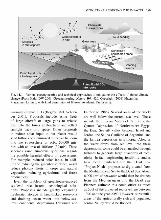
MITIGATION: REDUCING THE IMPACTS 189
Aerosolsin stratosphere
Giant reflectorsin orbit
Iron fertilization of sea
Pump liquid CO2into deep sea
Grow trees
Chemicalsto save ozone
Cloud seeding
Geneticallyengineered crops
Greeningdeserts
Drain ocean
Pump liquid CO2into rocks
Fig. 11.1 Various geoengineering and technical approaches to mitigating the effects of global climatechange (From Keith DW 2001. Geoengineering. Nature 409: 420. Copyright (2001) MacmillanMagazines Limited, with kind permission of Kluwer Academic Publishers).
warming (Figure 11.1) (Begley 1991, Schnei-der 2001). Proposals include using fleetsof large aircraft or large guns to releasedust into the lower stratosphere and reflectsunlight back into space. Other proposalsto reduce solar input to our planet wouldsend billions of aluminized reflective balloonsinto the stratosphere or orbit 50,000 mir-rors with an area of 100 km2 (39 mi2). Theseschemes raise numerous questions regard-ing possible harmful effects on ecosystems.For example, reduced solar input, in addi-tion to reducing the greenhouse effect, mightreduce photosynthesis in crops and naturalvegetation, reducing agricultural and forestproductivity.
Even the problem of greenhouse-inducedsea-level rise fosters technological solu-tions. Proposals include greatly expandingfreshwater storage in land-locked reservoirsand draining ocean water into below-sea-level continental depressions (Newman and
Fairbridge 1986). Several areas of the worldare well below the current sea level. Theseinclude the Imperial Valley of California, theQattara Depression of Northwestern Egypt,the Dead Sea rift valley between Israel andJordan, the Salina Gaulicho of Argentina, andthe Eritrea depression in Ethiopia. Also, asthe water drops from sea level into thesedepressions, some could be channeled throughturbines to generate large quantities of elec-tricity. In fact, engineering feasibility studieshave been conducted for the Dead Sea.“Project Noah” proposes to dig a canal fromthe Mediterranean Sea to the Dead Sea. About6,000 km2 of seawater would then be drainedfrom the Mediterranean into the Dead Sea.Planners estimate this could offset as muchas 50% of the projected sea-level rise between1990 and the year 2050. However, substantialareas of the agriculturally rich and populatedJordan Valley would be flooded.
190 CLIMATE CHANGE
Large-scale technological fixes to environ-mental problems such as greenhouse warm-ing should not be ignored. Further researchmay discover an effective and at least par-tial solution. However, even if possible, theirhigh cost generally makes them economicallyunfeasible. Furthermore, technology has cre-ated these problems and changed our planetin ways we do not fully understand. In ourrush to find a “quick fix” for the problemswe have created, we must be careful not tocreate additional problems. Such technologi-cal approaches deal with the end results, ratherthan the root cause (world dependence on fos-sil fuel) of global greenhouse warming.
Enhance Natural Carbon Sinks
If natural sinks of CO2 could be enlarged,they would remove more CO2 from the atmo-sphere. The ocean’s role as a significantsink for CO2 might be enhanced (Chapters 1and 8). Phytoplankton, in the lighted sur-face layers of the ocean, assimilate dissolvedCO2, and through photosynthesis, convert it toorganic carbon (biomass). Also, some species,most notably the coccolithophores, use CO2
to build exoskeletons of solid CaCO3 (cal-cium carbonate). When phytoplankton die,they sink, and a proportion of the fixedcarbon is removed to the deep ocean forlong-term (>200 years) storage. Phytoplank-ton, like other plants, require nutrients forgrowth. One nutrient that often limits thegrowth of oceanic phytoplankton is iron. Theexperimental addition of iron to small vol-umes of seawater often stimulates a rapidgrowth or bloom of phytoplankton.
Some scientists give serious considera-tion to the idea of dumping large quan-tities of iron into the ocean to stimulatealgal blooms and promote the removal ofdissolved CO2 to the deep ocean. In pilotexperiments (IRONEX) in the Pacific and
Antarctic Ocean, tons of iron were dumpedfrom ships and the effects on phytoplank-ton monitored (Monastersky 1995, Boyd et al.2000). The plankton bloomed, but the effectswere transient and disappointing. However,some researchers believe this approach isworth pursuing and patents for ocean fertil-ization procedures have been filed in anticipa-tion of a global market for carbon mitigationcredits.
To be effective on a large scale, such ascheme would need to involve hundreds, ifnot thousands, of ships dumping iron fulltime, and would be exceedingly costly. Also,adding iron to the ocean would probablycause a major change in the structure of openocean ecosystems that support fish, includ-ing those fish that are commercially har-vested. Nevertheless, the debate continueswithin the scientific community as to whetherthis scheme represents a feasible and worth-while mitigation option (Johnson and Karl2002) or a misguided and possibly danger-ous alteration of ocean systems (Chisholmet al. 2001).
Forest carbon sinks could be enhanced.Trees, through photosynthesis, remove CO2
from the atmosphere and store it as organiccarbon until the tree dies and decays, or isburned, releasing the carbon back into theatmosphere as CO2. The World’s vegetationand forests currently store about 610 Gt ofcarbon. Young growing forests shift carbonfrom the atmosphere into temporarily storedorganic biomass, but a mature old-growth for-est is probably close to equilibrium, giving offas much carbon to the atmosphere (as trees dieand decay) as it removes through photosyn-thesis. Planting a new tree could effectivelyoffset some CO2 emissions for the life ofthe tree, often 100 to 300 years, and large-scale reforestation could significantly reducethe rate of CO2 buildup in the atmosphere.
MITIGATION: REDUCING THE IMPACTS 191
If we could double our current rate of refor-estation each year, we could delay greenhousewarming for a decade or two, possiblylong enough to develop alternative sourcesof energy (Botkin 1989). Estimates for theUnited States suggest that reforestation of30 million hectares of economically marginalcrop, pasture, and non-Federal forest land(about 3% of US land area) could sequesterabout 5% of 1990 US CO2 emissions at a costof $7 per ton of CO2. Large-scale reforesta-tion will be difficult and expensive. It may bedifficult to find large enough areas suitablefor reforestation on this scale (Rubin et al.1992). However, reforestation should formone component of a broad strategy to addressgreenhouse warming. Again, caution is calledfor. Some scientists suggest that more forestscould decrease the Earth’s albedo so that thedarker surface would absorb more heat andadd to global warming.
Convert to Carbon-Free andRenewable Energy Technologies
Alternative (renewable nonfossil fuel) energysources could significantly reduce greenhousegas (GHG) emissions. Many are alreadyproven and effective sources of energy, butthey are dwarfed in magnitude by our con-sumption of coal, oil, and gas. Hydroelec-tricity from rivers and streams currentlysupplies 20% of global electrical demand.However, many streams remain untapped andthis source could be expanded, particularlythrough the use of multiple small-stream gen-erators on local scales. The Three GorgesDam in China, the largest hydroelectric damin the world, when completed, will generate84 billion kWh of electricity – an amount ofenergy equivalent to 40 to 50 million tons ofcoal per year. However, dams and hydroelec-tric plants have their own set of environmen-tal impacts, ranging from human population
displacement (1.9 million people in the caseof Three Gorges) to interference with migrat-ing fish and decreased downstream water flowand sedimentation.
Wood and plant fiber represent biomassthat can be burned and converted to heatto warm buildings, drive steam turbines togenerate electricity, or power motor vehicles(US DOE 2002b). Wood burning for cookingand space heating is probably the oldestsource of energy used by humans. In theburning process, organic carbon is convertedto CO2 and released into the atmosphere.However, burning simply releases CO2 thatwas captured during photosynthesis. If thesame number of trees are replanted, there is nonet effect on atmospheric CO2 concentration.
Plants can also be fermented to produceliquid fuels. Wood fiber can be converted tomethyl alcohol and burned. Currently, mostmotor vehicles in Brazil run on 100% ethylalcohol, mostly derived from the fermentationof maize. Large-scale wood or fiber farms couldcapture solar energy and convert it into biomassfuel, thus reducing our reliance on fossil fuel.Biodiesel is a fuel made from vegetable oil, forexample, soybean oil or from modified usedrestaurant grease. It can be burned either pureor as a mixture with petroleum-derived dieselfuel in standard diesel engines. In Europe,34% of all cars currently have diesel engines,and biodiesel made from rapeseed (canola)oil is sold in over 1,000 stations in Germanyalone. Converting prime agricultural land fromfood production to fuel production is probablyundesirable. However, large areas of arid ormarginal land could be used to raise less-demanding biomass crops.
Wind, essentially a form of solar energydriven by differences in atmospheric pressurebetween one area and another, representsanother promising source of alternative power.Humans have used wind power for millennia.
192 CLIMATE CHANGE
Sailing ships traveled the world, carryinghumans and their cargo from one conti-nent to another. Windmills have been usedfor centuries to pump water and to drivelarge stone grinding wheels to mill grain.New technology provides an effective meansfor windmills to drive electrical genera-tors, and wind generators are being installedat locations around the globe (Box 11.1;Figure 11.2).
Large wind farms, consisting of hundredsof wind generators capable of generatingsignificant quantities of electricity are nowfairly common. There are over 35,000 wind tur-bines worldwide, providing over 12,000 MWof total global generating capacity (AWEA2002). In the United States, wind-generatedelectricity currently represents a small fractionof the total electrical capacity, but accordingto Battelle’s Pacific Northwest Laboratory,
Box 11.1 Wind power (From AWEA 2002. American Wind Energy Association. 122CStreet NW, Washington DC 2001. Available from: http://www.awea.org)
What is a wind turbine and how does it work?
A wind energy system transforms the kinetic energy of the wind into mechanical or electricalenergy that can be harnessed for practical use. Mechanical energy is most commonly usedfor pumping water in rural or remote locations. Wind electric turbines generate electricityfor homes and businesses and for sale to utilities. Turbine subsystems include
• a rotor, or blades, which convert the wind’s energy into rotational shaft energy;
• a nacelle (enclosure) containing a drive train, usually including a gearbox and a generator;
• a tower to support the rotor and drive train; and
• electronic equipment such as controls, electrical cables, ground support equipment, andinterconnection equipment.
How much electricity can one wind turbine generate?
The ability to generate electricity is measured in watts. Watts are very small units, sothe terms kilowatt (kW, 1,000 watts), megawatt (MW, 1 million watts), and gigawatt(GW = 1 billion watts) are most commonly used to describe the capacity of generatingunits such as wind turbines or other power plants.
Electricity production and consumption are most commonly measured in kilowatt-hours(kWh). A kilowatt-hour is one kilowatt (1,000 watts) of electricity produced or consumedfor one hour. One 50-W light bulb left on for 20 h consumes one kilowatt-hour of electricity(50 W × 20 h = 1,000 Wh = 1 kWh). Wind turbines being manufactured now have powerratings ranging from about 250 W to 1.8 megawatts (MW). The output of a wind turbinedepends on the turbine’s size and the wind’s speed through the rotor. A 10-m-diameterrotor would generate 25 kW or 45 MWh, while a 71-m rotor would produce 1,650 kW or5,600 MWh.

MITIGATION: REDUCING THE IMPACTS 193
A 10-kW wind turbine can generate about 16,000 kWh annually, more than enough topower a typical household. A 1.8-MW turbine can produce more than 5.2 million kWh in ayear – enough to power more than 500 households. The average US household consumesabout 10,000 kWh of electricity each year.
World Growth
Some 6,500 MW of new wind energy generating capacity were installed worldwide in 2001,amounting to annual sales of about $7 billion. This is the largest increase ever in globalwind energy installations, well above the capacity added in 2000 (3,800 MW) and 1999(3,900 MW). The world’s wind energy–generating capacity at the close of 2001 stood atabout 24,000 MW.
Germany set a world and national record of more than 2,600 MW of new generatingcapacity installed during the year. Germany, Denmark, and Spain are demonstrating thatwind can reliably provide 10 to 25% and more of a region or country’s electricity supply.
In the United States, the wind energy industry exceeded previous national records in2001, installing nearly 1,700 MW or $1.7 billion worth of new generating equipment. Thenew installations account for close to a third of the world wind energy generating capacityadded in 2001.
The global wind energy market continues to be dominated by the “big five” countries withover 1,000 MW of generating capacity each: Germany, the United States, Spain, Denmark,and India. The number of countries with several hundred megawatts is growing larger,however, and it may be that in the next several years – if the current rafts of proposedprojects are developed – Brazil and the United Kingdom will see their own wind-generatingcapacity exceed the 1,000-MW mark.
wind could potentially supply about 20% ofthe nation’s electricity. Furthermore, wind-generated electricity could be greatly ex-panded. A recent study performed by Den-mark’s BTM Consult for the European WindEnergy Association and Greenpeace found thatby the year 2017, wind could provide 10%of the world’s electricity. However, there arelimitations. Desirable wind-generating sites arelimited to those areas that have winds of con-sistent moderate to strong speed without strongmaxima and minima.
The huge potential energy of the Sun offersanother alternative to fossil fuel. The averageannual amount of solar energy reaching the
Earth’s surface (198 W m−2) far exceeds allcurrent human energy requirements. Withproper architectural design, passive solarspace heating of buildings could be greatlyexpanded. The feasibility of this low-techapproach is generally underestimated. It requi-res no new technology and can usuallybe accomplished for about the cost ofconventional building construction. It onlyrequires an adequate area of south-facingglass windows, proper roof overhang to shadesummer sun, good insulation, and some ther-mal mass such as concrete or water insidethe building for heat storage (Kachadorian1997). Even in northern temperate latitudes,
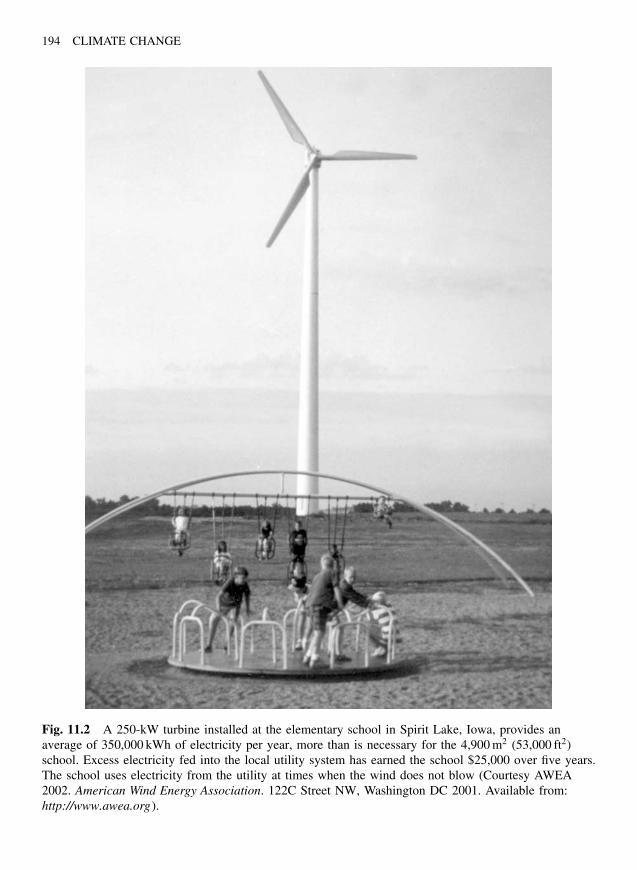
194 CLIMATE CHANGE
Fig. 11.2 A 250-kW turbine installed at the elementary school in Spirit Lake, Iowa, provides anaverage of 350,000 kWh of electricity per year, more than is necessary for the 4,900 m2 (53,000 ft2)school. Excess electricity fed into the local utility system has earned the school $25,000 over five years.The school uses electricity from the utility at times when the wind does not blow (Courtesy AWEA2002. American Wind Energy Association. 122C Street NW, Washington DC 2001. Available from:http://www.awea.org).
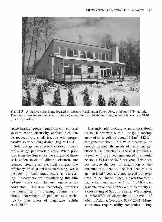
MITIGATION: REDUCING THE IMPACTS 195
Fig. 11.3 A passive solar home located in Western Washington State, USA, at about 48 ◦N latitude.The annual cost for supplemental (nonsolar) energy in this cloudy and rainy location is less than $150(Photo by author).
space-heating requirements from conventionalsources (wood, electricity, or fossil fuel) canbe reduced to a small fraction with properpassive solar building design (Figure 11.3).
Solar energy can also be converted to elec-tricity using photovoltaic cells. When pho-tons from the Sun strike the surface of thesecells (often made of silicon), electrons arereleased creating an electrical current. Theefficiency of solar cells is increasing, whilethe cost of their manufacture is decreas-ing. Researchers are investigating thin-film“plastic” solar cells that use organic semi-conductors. This new technology promisesthe possibility of increasing quantum effi-ciency (conversion of photons to electric-ity) by five orders of magnitude (Schonet al. 2000).
Currently, photovoltaic systems cost about$5 to $6 per watt output. Today, a rooftoparray of solar cells of about 13.2 m2 (142 ft2)can generate about 1,500 W of electricity, orenough to meet the needs of many energy-efficient US households. The cost for such asystem with a 20-year guaranteed life wouldbe about $9,000 or $428 per year. This doesnot include the cost of installation or thediscount rate, that is, the fact that this isan “up-front” cost and not spread out overtime. In the United States, a fixed (nonrotat-ing) solar panel area of 45 m2 (484 ft2) cangenerate an annual 4,899 kWh of electricity ata cost saving of $250 in Seattle, Washington,or 6,786 kWh of electricity at a saving of$461 in Atlanta, Georgia (NCPV 2002). Manystates now require utility companies to buy
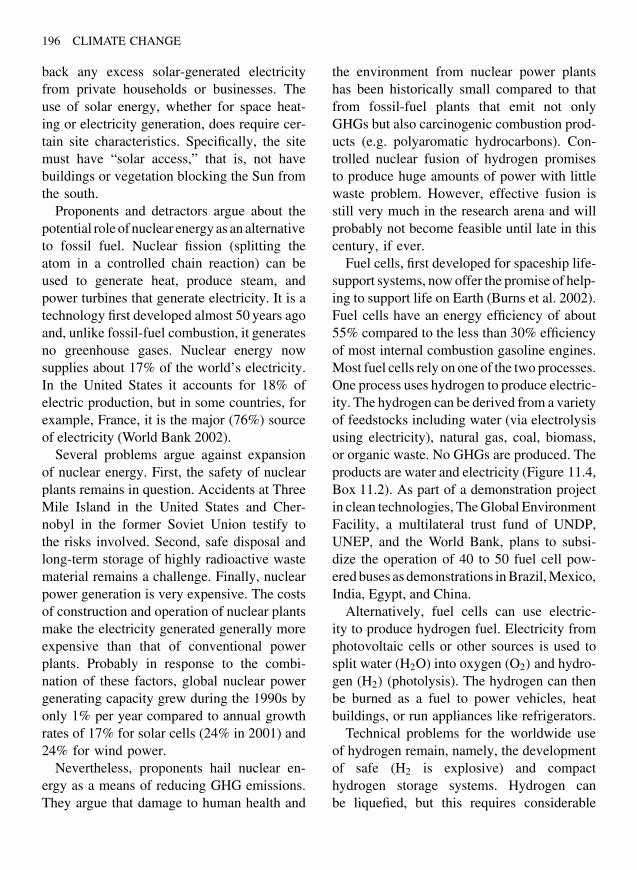
196 CLIMATE CHANGE
back any excess solar-generated electricityfrom private households or businesses. Theuse of solar energy, whether for space heat-ing or electricity generation, does require cer-tain site characteristics. Specifically, the sitemust have “solar access,” that is, not havebuildings or vegetation blocking the Sun fromthe south.
Proponents and detractors argue about thepotential role of nuclear energy as an alternativeto fossil fuel. Nuclear fission (splitting theatom in a controlled chain reaction) can beused to generate heat, produce steam, andpower turbines that generate electricity. It is atechnology first developed almost 50 years agoand, unlike fossil-fuel combustion, it generatesno greenhouse gases. Nuclear energy nowsupplies about 17% of the world’s electricity.In the United States it accounts for 18% ofelectric production, but in some countries, forexample, France, it is the major (76%) sourceof electricity (World Bank 2002).
Several problems argue against expansionof nuclear energy. First, the safety of nuclearplants remains in question. Accidents at ThreeMile Island in the United States and Cher-nobyl in the former Soviet Union testify tothe risks involved. Second, safe disposal andlong-term storage of highly radioactive wastematerial remains a challenge. Finally, nuclearpower generation is very expensive. The costsof construction and operation of nuclear plantsmake the electricity generated generally moreexpensive than that of conventional powerplants. Probably in response to the combi-nation of these factors, global nuclear powergenerating capacity grew during the 1990s byonly 1% per year compared to annual growthrates of 17% for solar cells (24% in 2001) and24% for wind power.
Nevertheless, proponents hail nuclear en-ergy as a means of reducing GHG emissions.They argue that damage to human health and
the environment from nuclear power plantshas been historically small compared to thatfrom fossil-fuel plants that emit not onlyGHGs but also carcinogenic combustion prod-ucts (e.g. polyaromatic hydrocarbons). Con-trolled nuclear fusion of hydrogen promisesto produce huge amounts of power with littlewaste problem. However, effective fusion isstill very much in the research arena and willprobably not become feasible until late in thiscentury, if ever.
Fuel cells, first developed for spaceship life-support systems, now offer the promise of help-ing to support life on Earth (Burns et al. 2002).Fuel cells have an energy efficiency of about55% compared to the less than 30% efficiencyof most internal combustion gasoline engines.Most fuel cells rely on one of the two processes.One process uses hydrogen to produce electric-ity. The hydrogen can be derived from a varietyof feedstocks including water (via electrolysisusing electricity), natural gas, coal, biomass,or organic waste. No GHGs are produced. Theproducts are water and electricity (Figure 11.4,Box 11.2). As part of a demonstration projectin clean technologies, The Global EnvironmentFacility, a multilateral trust fund of UNDP,UNEP, and the World Bank, plans to subsi-dize the operation of 40 to 50 fuel cell pow-ered buses as demonstrations in Brazil, Mexico,India, Egypt, and China.
Alternatively, fuel cells can use electric-ity to produce hydrogen fuel. Electricity fromphotovoltaic cells or other sources is used tosplit water (H2O) into oxygen (O2) and hydro-gen (H2) (photolysis). The hydrogen can thenbe burned as a fuel to power vehicles, heatbuildings, or run appliances like refrigerators.
Technical problems for the worldwide useof hydrogen remain, namely, the developmentof safe (H2 is explosive) and compacthydrogen storage systems. Hydrogen canbe liquefied, but this requires considerable
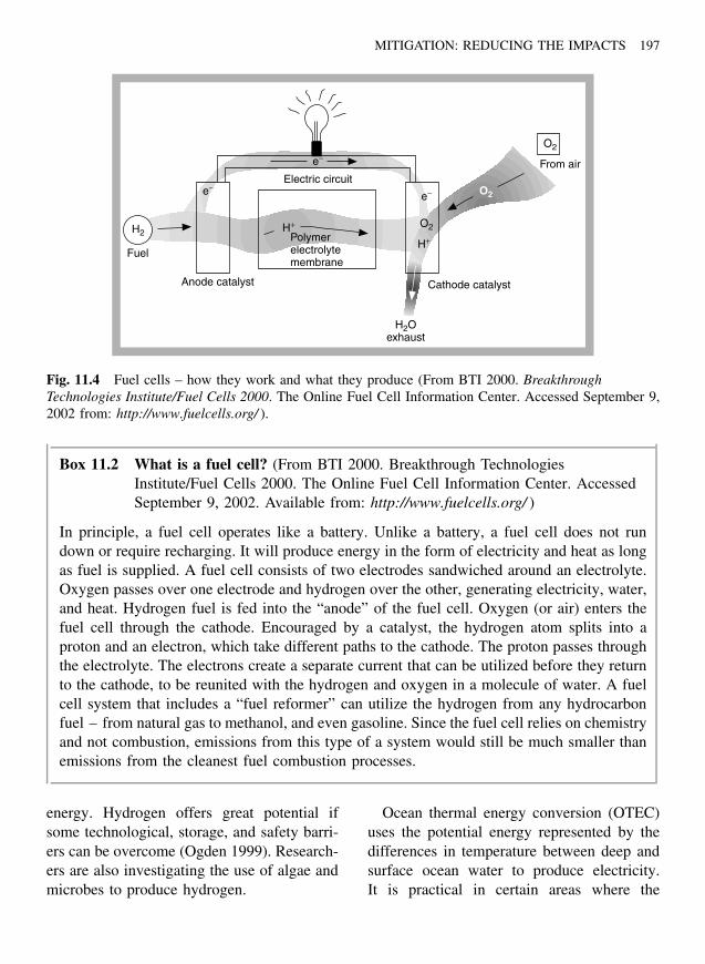
MITIGATION: REDUCING THE IMPACTS 197
Anode catalyst
Fuel
H2
H2Oexhaust
O2
From air
Cathode catalyst
Electric circuit
e−
H+
Polymerelectrolytemembrane
e−e−
O2
H+
O2
Fig. 11.4 Fuel cells – how they work and what they produce (From BTI 2000. BreakthroughTechnologies Institute/Fuel Cells 2000. The Online Fuel Cell Information Center. Accessed September 9,2002 from: http://www.fuelcells.org/ ).
Box 11.2 What is a fuel cell? (From BTI 2000. Breakthrough TechnologiesInstitute/Fuel Cells 2000. The Online Fuel Cell Information Center. AccessedSeptember 9, 2002. Available from: http://www.fuelcells.org/ )
In principle, a fuel cell operates like a battery. Unlike a battery, a fuel cell does not rundown or require recharging. It will produce energy in the form of electricity and heat as longas fuel is supplied. A fuel cell consists of two electrodes sandwiched around an electrolyte.Oxygen passes over one electrode and hydrogen over the other, generating electricity, water,and heat. Hydrogen fuel is fed into the “anode” of the fuel cell. Oxygen (or air) enters thefuel cell through the cathode. Encouraged by a catalyst, the hydrogen atom splits into aproton and an electron, which take different paths to the cathode. The proton passes throughthe electrolyte. The electrons create a separate current that can be utilized before they returnto the cathode, to be reunited with the hydrogen and oxygen in a molecule of water. A fuelcell system that includes a “fuel reformer” can utilize the hydrogen from any hydrocarbonfuel – from natural gas to methanol, and even gasoline. Since the fuel cell relies on chemistryand not combustion, emissions from this type of a system would still be much smaller thanemissions from the cleanest fuel combustion processes.
energy. Hydrogen offers great potential ifsome technological, storage, and safety barri-ers can be overcome (Ogden 1999). Research-ers are also investigating the use of algae andmicrobes to produce hydrogen.
Ocean thermal energy conversion (OTEC)uses the potential energy represented by thedifferences in temperature between deep andsurface ocean water to produce electricity.It is practical in certain areas where the

198 CLIMATE CHANGE
temperature difference between warm surfacewater and deep water differs by at least 20 ◦C.In an open-cycle OTEC system, warm seawa-ter is “flash” evaporated in a vacuum chamberto produce steam. The steam expands througha low-pressure turbine that is coupled to agenerator to produce electricity. The steamexiting the turbine is condensed by cold sea-water pumped from the ocean’s depths. Ifa surface condenser is used in the system,the condensed steam remains separated fromthe cold seawater and provides a supply ofdesalinated water (Figure 11.5). The technol-ogy was field-tested in Hawaii in 1993, wherean OTEC plant at Keahole Point, Hawaii, pro-duced 50,000 W of electricity. The potentialis great, but considerable research needs tobe completed before this technology becomespractical. Nevertheless, OTEC could providepower to selected coastal or island communi-ties located near deep water (NREL 2002).
Lunar and solar cycles drive ocean tides,and winds create ocean surface waves. Tidalenergy can be exploited in two ways. “Bar-rages” allow tidal waters to fill an estuaryvia sluices and to empty through turbines.Tidal streams harness offshore underwatertidal currents with devices similar to windturbines. Both are limited to areas that expe-rience high tidal ranges. Tidal stream tech-nology is in its infancy, with only oneprototype 5-kW machine operational in theworld. The exploitable tidal energy poten-tial in Europe is 105 TWh year−1 (TWh =terawatt hours = 1012 watt hours) from tidalbarrages (mostly in France and the UnitedKingdom) and 48 TWh year−1 from tidalstream turbines (mostly around UK shores).A 240-MW barrage has been operational atLa Rance in France since 1967. Both tech-nologies are currently not economically com-petitive with other forms of energy and nofurther deployments are anticipated before
2010 (E.C. 2002). Also, tidal energy schemesaffect the environment, influencing water lev-els, currents, and sediment transport.
Ocean waves contain huge amounts ofenergy (Falnes and Lovseth 1991). Wavesare another form of stored solar energy,since the winds that produce waves arecaused by pressure differences in the atmo-sphere arising from solar heating. Globally,total wave power generating potential isabout 2,000 TWh year−1 (E.C. 2002) or morethan 150 times more energy than the totalglobal electrical consumption of 13.7 TWhfor the year 2,000 (US DOE 2002c). Waveenergy potentials in the European Union areaalone have been estimated conservatively at120 to 190 TWh year−1 (offshore) and 34 to46 TWh year−1 (nearshore).
A great variety of wave energy deviceshave been proposed and several have beendeployed in the sea as prototypes ordemonstration schemes. The pendulum device(Figure 11.6a) consists of a rectangular boxthat is open to the sea at one end. Apendulum flap is hinged over this opening,so that the action of the waves causes itto swing back and forth. This motion isthen used to power a hydraulic pump andgenerator. Only small devices have beendeployed and tested. Another example is theoscillating water column device composedof a partly submerged concrete or steelstructure, which has an opening to the seabelow the water line, thereby enclosing acolumn of air above a column of water. Aswaves impinge on the device, they causethe water column to rise and fall, whichalternately compresses and depressurizes theair column (Figure 11.6b). This air is allowedto flow to and from the atmosphere througha turbine, which drives an electric generator.The tapered channel system (Figure 11.6c)consists of a gradually narrowing channel

MITIGATION: REDUCING THE IMPACTS 199
Warmseawater in
Noncondensablegases
Coldseawaterdischarge
to sea
Desalinatedwater
(optional)
Coldseawater inWarm
seawaterdischarge
to sea
Noncondensablegases
Desalinatedwater vapor
(unsaturated)
Desalinatedwater vapor(saturated)
Deaeration(optional)
Turbo-generator Condenser
Vacuumchamber
flashevaporator
(a)
HMTEA/NPPEOpen-cycle
OTEC system
Misteliminator
Diffuser
Spoutevaporator
Drains
Supplies
Warm
Warm
Cold
Cold
Synchronousgenerator
Steam
Radial inflowturbine
Directcontactcondenser
Vacuumexhaust
(b)
Fig. 11.5 An open-cycle ocean thermal energy conversion system (OTEC). In tropical waters, oceansurface temperatures may reach 80 ◦F, while at depths of 5,000 feet, temperatures are near freezing.Warm surface water is pumped to a vacuum chamber to produce steam that drives a turbine. At thesame time, a heat exchanger uses cold water pumped from depths to condense spent steam intodrinkable water (Part (a) reproduced with permission of U.S. Department of Energy, NationalRenewable Energy Laboratory, Golden, Colorado, USA http://www.nrel.gov/otec/).
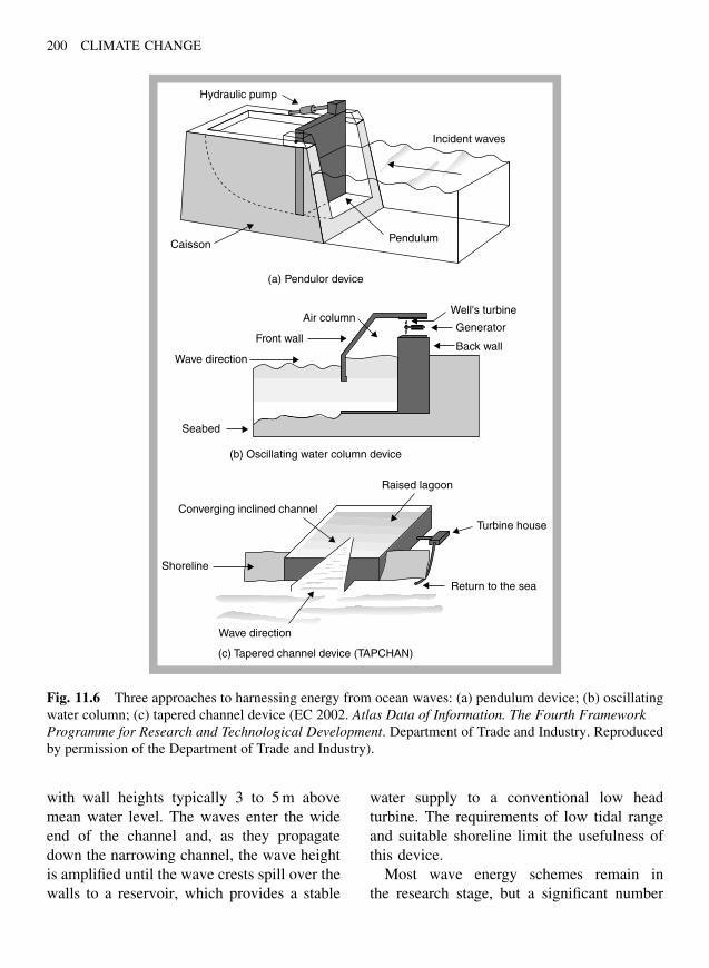
200 CLIMATE CHANGE
Hydraulic pump
Incident waves
PendulumCaisson
(a) Pendulor device
(b) Oscillating water column device
(c) Tapered channel device (TAPCHAN)
Converging inclined channel
Air column
Front wall
Wave direction
Seabed
Well's turbine
Generator
Back wall
Raised lagoon
Turbine house
Return to the sea
Wave direction
Shoreline
Fig. 11.6 Three approaches to harnessing energy from ocean waves: (a) pendulum device; (b) oscillatingwater column; (c) tapered channel device (EC 2002. Atlas Data of Information. The Fourth FrameworkProgramme for Research and Technological Development. Department of Trade and Industry. Reproducedby permission of the Department of Trade and Industry).
with wall heights typically 3 to 5 m abovemean water level. The waves enter the wideend of the channel and, as they propagatedown the narrowing channel, the wave heightis amplified until the wave crests spill over thewalls to a reservoir, which provides a stable
water supply to a conventional low headturbine. The requirements of low tidal rangeand suitable shoreline limit the usefulness ofthis device.
Most wave energy schemes remain inthe research stage, but a significant number
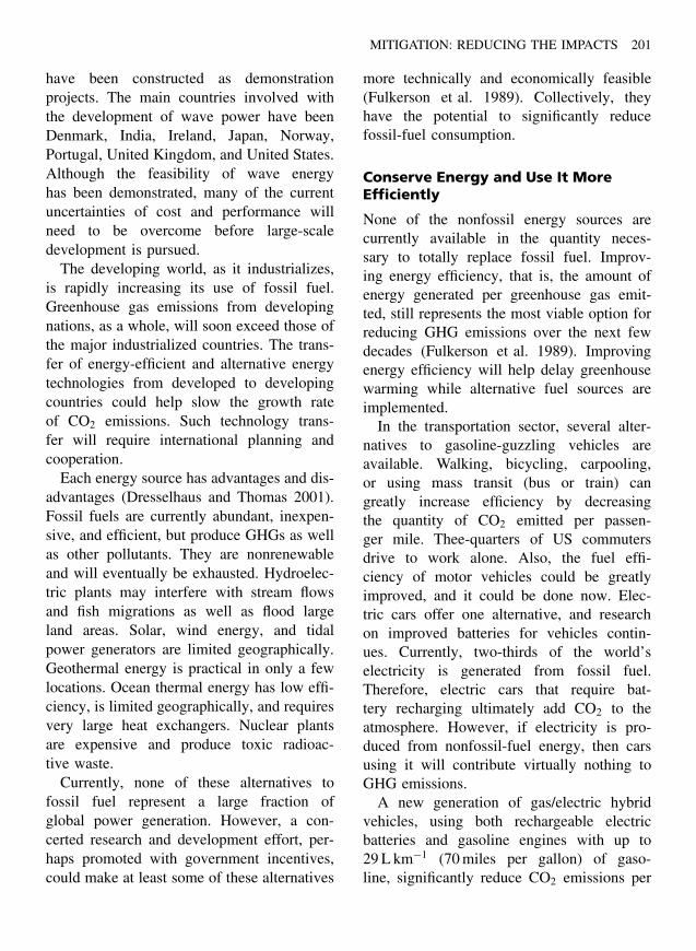
MITIGATION: REDUCING THE IMPACTS 201
have been constructed as demonstrationprojects. The main countries involved withthe development of wave power have beenDenmark, India, Ireland, Japan, Norway,Portugal, United Kingdom, and United States.Although the feasibility of wave energyhas been demonstrated, many of the currentuncertainties of cost and performance willneed to be overcome before large-scaledevelopment is pursued.
The developing world, as it industrializes,is rapidly increasing its use of fossil fuel.Greenhouse gas emissions from developingnations, as a whole, will soon exceed those ofthe major industrialized countries. The trans-fer of energy-efficient and alternative energytechnologies from developed to developingcountries could help slow the growth rateof CO2 emissions. Such technology trans-fer will require international planning andcooperation.
Each energy source has advantages and dis-advantages (Dresselhaus and Thomas 2001).Fossil fuels are currently abundant, inexpen-sive, and efficient, but produce GHGs as wellas other pollutants. They are nonrenewableand will eventually be exhausted. Hydroelec-tric plants may interfere with stream flowsand fish migrations as well as flood largeland areas. Solar, wind energy, and tidalpower generators are limited geographically.Geothermal energy is practical in only a fewlocations. Ocean thermal energy has low effi-ciency, is limited geographically, and requiresvery large heat exchangers. Nuclear plantsare expensive and produce toxic radioac-tive waste.
Currently, none of these alternatives tofossil fuel represent a large fraction ofglobal power generation. However, a con-certed research and development effort, per-haps promoted with government incentives,could make at least some of these alternatives
more technically and economically feasible(Fulkerson et al. 1989). Collectively, theyhave the potential to significantly reducefossil-fuel consumption.
Conserve Energy and Use It MoreEfficiently
None of the nonfossil energy sources arecurrently available in the quantity neces-sary to totally replace fossil fuel. Improv-ing energy efficiency, that is, the amount ofenergy generated per greenhouse gas emit-ted, still represents the most viable option forreducing GHG emissions over the next fewdecades (Fulkerson et al. 1989). Improvingenergy efficiency will help delay greenhousewarming while alternative fuel sources areimplemented.
In the transportation sector, several alter-natives to gasoline-guzzling vehicles areavailable. Walking, bicycling, carpooling,or using mass transit (bus or train) cangreatly increase efficiency by decreasingthe quantity of CO2 emitted per passen-ger mile. Thee-quarters of US commutersdrive to work alone. Also, the fuel effi-ciency of motor vehicles could be greatlyimproved, and it could be done now. Elec-tric cars offer one alternative, and researchon improved batteries for vehicles contin-ues. Currently, two-thirds of the world’selectricity is generated from fossil fuel.Therefore, electric cars that require bat-tery recharging ultimately add CO2 to theatmosphere. However, if electricity is pro-duced from nonfossil-fuel energy, then carsusing it will contribute virtually nothing toGHG emissions.
A new generation of gas/electric hybridvehicles, using both rechargeable electricbatteries and gasoline engines with up to29 L km−1 (70 miles per gallon) of gaso-line, significantly reduce CO2 emissions per
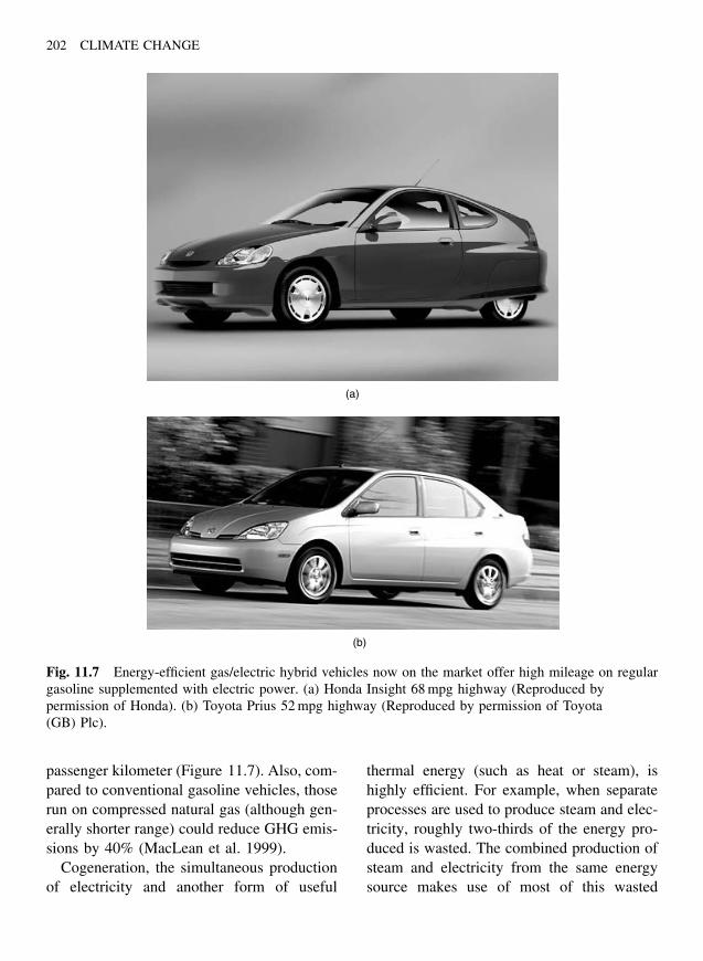
202 CLIMATE CHANGE
(a)
(b)
Fig. 11.7 Energy-efficient gas/electric hybrid vehicles now on the market offer high mileage on regulargasoline supplemented with electric power. (a) Honda Insight 68 mpg highway (Reproduced bypermission of Honda). (b) Toyota Prius 52 mpg highway (Reproduced by permission of Toyota(GB) Plc).
passenger kilometer (Figure 11.7). Also, com-pared to conventional gasoline vehicles, thoserun on compressed natural gas (although gen-erally shorter range) could reduce GHG emis-sions by 40% (MacLean et al. 1999).
Cogeneration, the simultaneous productionof electricity and another form of useful
thermal energy (such as heat or steam), ishighly efficient. For example, when separateprocesses are used to produce steam and elec-tricity, roughly two-thirds of the energy pro-duced is wasted. The combined production ofsteam and electricity from the same energysource makes use of most of this wasted
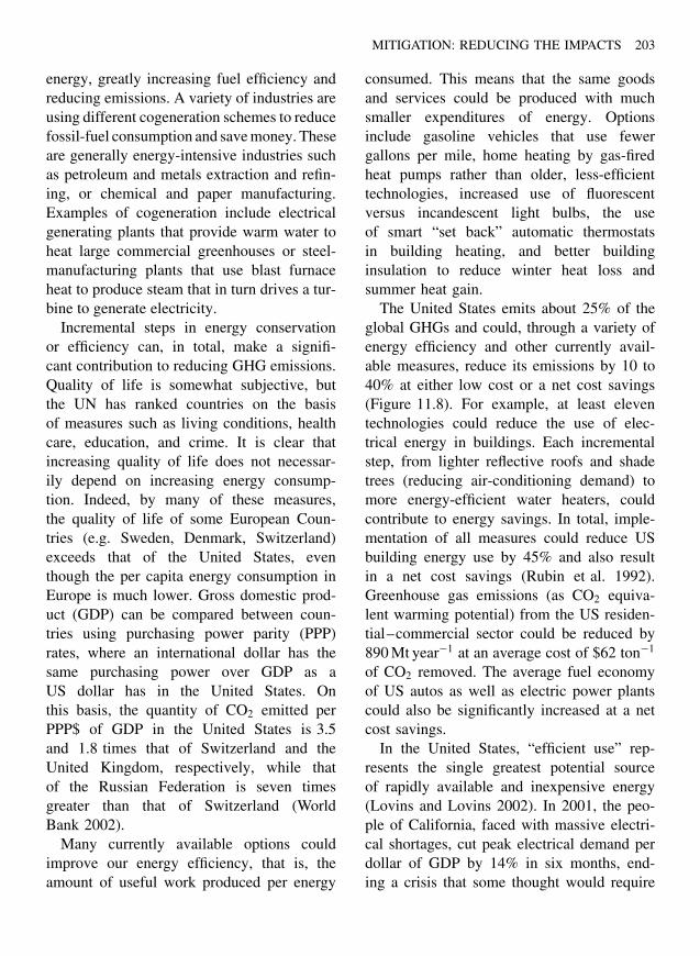
MITIGATION: REDUCING THE IMPACTS 203
energy, greatly increasing fuel efficiency andreducing emissions. A variety of industries areusing different cogeneration schemes to reducefossil-fuel consumption and save money. Theseare generally energy-intensive industries suchas petroleum and metals extraction and refin-ing, or chemical and paper manufacturing.Examples of cogeneration include electricalgenerating plants that provide warm water toheat large commercial greenhouses or steel-manufacturing plants that use blast furnaceheat to produce steam that in turn drives a tur-bine to generate electricity.
Incremental steps in energy conservationor efficiency can, in total, make a signifi-cant contribution to reducing GHG emissions.Quality of life is somewhat subjective, butthe UN has ranked countries on the basisof measures such as living conditions, healthcare, education, and crime. It is clear thatincreasing quality of life does not necessar-ily depend on increasing energy consump-tion. Indeed, by many of these measures,the quality of life of some European Coun-tries (e.g. Sweden, Denmark, Switzerland)exceeds that of the United States, eventhough the per capita energy consumption inEurope is much lower. Gross domestic prod-uct (GDP) can be compared between coun-tries using purchasing power parity (PPP)rates, where an international dollar has thesame purchasing power over GDP as aUS dollar has in the United States. Onthis basis, the quantity of CO2 emitted perPPP$ of GDP in the United States is 3.5and 1.8 times that of Switzerland and theUnited Kingdom, respectively, while thatof the Russian Federation is seven timesgreater than that of Switzerland (WorldBank 2002).
Many currently available options couldimprove our energy efficiency, that is, theamount of useful work produced per energy
consumed. This means that the same goodsand services could be produced with muchsmaller expenditures of energy. Optionsinclude gasoline vehicles that use fewergallons per mile, home heating by gas-firedheat pumps rather than older, less-efficienttechnologies, increased use of fluorescentversus incandescent light bulbs, the useof smart “set back” automatic thermostatsin building heating, and better buildinginsulation to reduce winter heat loss andsummer heat gain.
The United States emits about 25% of theglobal GHGs and could, through a variety ofenergy efficiency and other currently avail-able measures, reduce its emissions by 10 to40% at either low cost or a net cost savings(Figure 11.8). For example, at least eleventechnologies could reduce the use of elec-trical energy in buildings. Each incrementalstep, from lighter reflective roofs and shadetrees (reducing air-conditioning demand) tomore energy-efficient water heaters, couldcontribute to energy savings. In total, imple-mentation of all measures could reduce USbuilding energy use by 45% and also resultin a net cost savings (Rubin et al. 1992).Greenhouse gas emissions (as CO2 equiva-lent warming potential) from the US residen-tial–commercial sector could be reduced by890 Mt year−1 at an average cost of $62 ton−1
of CO2 removed. The average fuel economyof US autos as well as electric power plantscould also be significantly increased at a netcost savings.
In the United States, “efficient use” rep-resents the single greatest potential sourceof rapidly available and inexpensive energy(Lovins and Lovins 2002). In 2001, the peo-ple of California, faced with massive electri-cal shortages, cut peak electrical demand perdollar of GDP by 14% in six months, end-ing a crisis that some thought would require

204 CLIMATE CHANGE
0
8
6
4
2
00 10 20 30 40 50
100 200 300Reduction in CO2 emissions (MT/yr−1)
Percent savings in building electricity use
1. White roofs & trees2. Residential lighting-replace with compact fluorescents3. More efficient residential water heaters4. More efficient commercial water heating5. Commercial lighting6. Commercial cooking7. Commercial cooling8. Commercial refrigeration9. Residential appliances10. Residential space heating11. Comm & indust. space heating12. Comm. ventilation and fuel efficiency
Cos
t of e
lect
ricity
effi
cien
cy m
easu
res
(cen
ts/k
Wh−1
)
Net
impl
emen
tatio
n co
st
All-sector electricity price (1989) = 6.4 cents/kWh
400 500
20
0
−20
−40
−60
−80
12
3 4 5 67
8
910
11
12
3%
6%
d = 10%
Fig. 11.8 Currently available technological changes in 12 different end uses of electricity could reducebuilding energy use by 734 billion kWh or 45% of the US demand at a net cost savings. Each step is theannualized investment cost of a given technological option numbered at left. For example, white roofsand trees (1) could decrease air-conditioning requirements, and reduce CO2 emissions by 40 mt year−1,saving 4% in building electrical use and 0.5 cents per kWh (Reprinted with permission from Rubin ES,Cooper RN, Frosch RA, Lee TH, Marland G, Rosenfeld AH, et al. 1992. Realistic mitigation options forglobal warming. Science 257: 148–149 & 261–266. Copyright (1992) American Association for theAdvancement of Science).
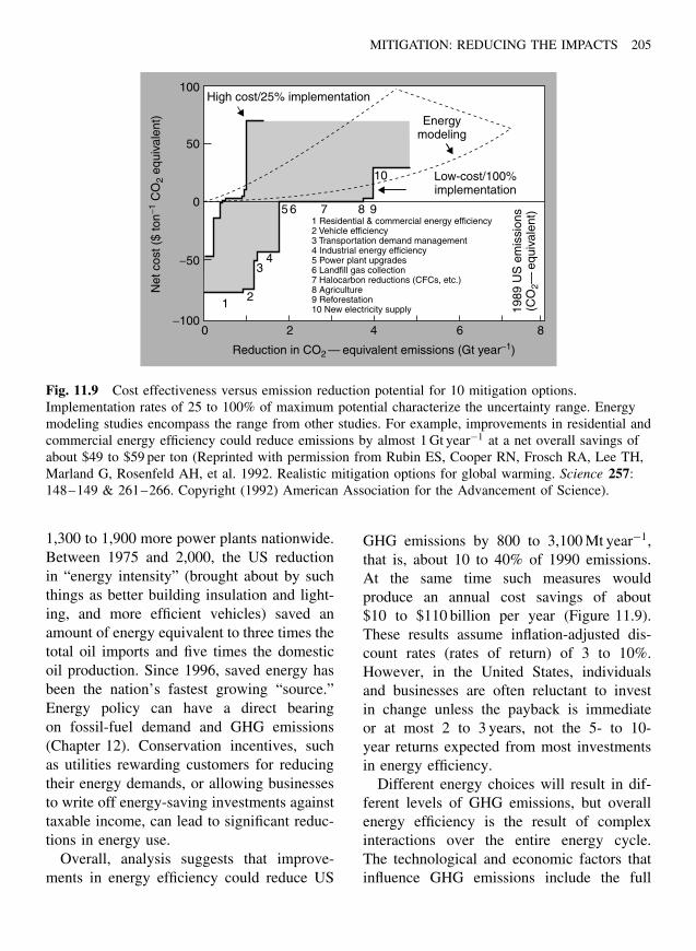
MITIGATION: REDUCING THE IMPACTS 205
100High cost/25% implementation
1 Residential & commercial energy efficiency2 Vehicle efficiency3 Transportation demand management4 Industrial energy efficiency5 Power plant upgrades6 Landfill gas collection7 Halocarbon reductions (CFCs, etc.)8 Agriculture9 Reforestation10 New electricity supply
50
−50
−1000 2 4
Reduction in CO2 — equivalent emissions (Gt year−1)
Net
cos
t ($
ton−1
CO
2 eq
uiva
lent
)
6 8
0
Energymodeling
Low-cost/100%implementation
1989
US
em
issi
ons
(CO
2—eq
uiva
lent
)
10
98765
43
21
Fig. 11.9 Cost effectiveness versus emission reduction potential for 10 mitigation options.Implementation rates of 25 to 100% of maximum potential characterize the uncertainty range. Energymodeling studies encompass the range from other studies. For example, improvements in residential andcommercial energy efficiency could reduce emissions by almost 1 Gt year−1 at a net overall savings ofabout $49 to $59 per ton (Reprinted with permission from Rubin ES, Cooper RN, Frosch RA, Lee TH,Marland G, Rosenfeld AH, et al. 1992. Realistic mitigation options for global warming. Science 257:148–149 & 261–266. Copyright (1992) American Association for the Advancement of Science).
1,300 to 1,900 more power plants nationwide.Between 1975 and 2,000, the US reductionin “energy intensity” (brought about by suchthings as better building insulation and light-ing, and more efficient vehicles) saved anamount of energy equivalent to three times thetotal oil imports and five times the domesticoil production. Since 1996, saved energy hasbeen the nation’s fastest growing “source.”Energy policy can have a direct bearingon fossil-fuel demand and GHG emissions(Chapter 12). Conservation incentives, suchas utilities rewarding customers for reducingtheir energy demands, or allowing businessesto write off energy-saving investments againsttaxable income, can lead to significant reduc-tions in energy use.
Overall, analysis suggests that improve-ments in energy efficiency could reduce US
GHG emissions by 800 to 3,100 Mt year−1,that is, about 10 to 40% of 1990 emissions.At the same time such measures wouldproduce an annual cost savings of about$10 to $110 billion per year (Figure 11.9).These results assume inflation-adjusted dis-count rates (rates of return) of 3 to 10%.However, in the United States, individualsand businesses are often reluctant to investin change unless the payback is immediateor at most 2 to 3 years, not the 5- to 10-year returns expected from most investmentsin energy efficiency.
Different energy choices will result in dif-ferent levels of GHG emissions, but overallenergy efficiency is the result of complexinteractions over the entire energy cycle.The technological and economic factors thatinfluence GHG emissions include the full
206 CLIMATE CHANGE
fuel cycle, that is, conversion from theprimary energy source to actual end useincluding different conversion, transport, andend-use systems (Nakic′enovic′ 1993). Inthe industrialized countries, energy intensity(watts year−1 dollar−1) has been increasingabout 1% per year since the 1860s. Inaddition, energy use has undergone “decar-bonization,” that is, a shift from fuels ofhigh carbon content (coal) to those oflower carbon content such as oil, naturalgas, or carbon-free nuclear energy. How-ever, with economic output increasing at3% per year, the improvement in inten-sity will not keep pace with the growthin CO2 emissions. Computer models of thefull fuel cycle suggest that choices in howa service (e.g. building lighting) is pro-vided can result in differences in CO2 emis-sions of 90%. Thus, CO2 emissions couldbe reduced substantially using currently avail-able technology.
Adapt to Climate Change
Even if GHG emissions were drasticallyreduced today, the Earth’s climate wouldprobably continue to warm for some time.Regardless of the rate of fossil-fuel com-bustion, if all the known fossil-fuel reserves(about 4,000 GtC) are burned, CO2 will reachabout 1,000 ppmv and the Earth will bewarmed by >5 ◦C by the end of the mil-lennium (Lenton and Cannell 2002). Hence,some scientists and politicians argue that wemust prepare to adapt to the inevitable cli-mate change. Research funded by the ElectricPower Research Institute suggests that a vari-ety of adaptation measures, from better build-ing insulation to altered crop species, couldbe instituted to lessen the impacts of climatechange on a variety of sectors (Table 11.1).
Adaptation can be effective, especially ifthe value of the resulting benefit is greater
than the cost of the adaptation. The net eco-nomic impact of climate change may belessened in the case of efficient adaptationmeasures, but may be increased by inefficientmeasures. Building new seawalls to protectagainst sea-level rise can be very expensive,but if it saves a valuable tourist beach or thehomes of many people, then it may be worth-while. On the other hand, investing billionsin fossil fuel–powered air conditioning mightbring some reduction in medical costs asso-ciated with heatstroke, but it could add evenmore to a variety of costs related to furtherGHG emissions and global warming. Adap-tation obviously does not solve the long-termproblem of damage and increased costs fromcontinued GHG emissions.
Taking ActionMany actions can be taken that wouldgreatly reduce GHG emissions and or reducethe impacts of greenhouse warming. Theseactions can be undertaken globally, nationally,and individually. Policies related to energyand GHG emissions are discussed morefully in Chapter 12. Globally, we need tostrengthen and adhere to international treatieson climate change. The climate problem isglobal and its mitigation will require inter-national cooperation. Although US delegatessigned the 1997 Kyoto Protocol (Chapter 12),Congress never ratified the treaty, and theUnited States has fallen far short of the emis-sion reduction goals it agreed to in Kyoto.
Nationally, individual countries need toinstitute good faith efforts of their own, per-haps going beyond international agreementsto mitigate as much as they possibly can. Car-bon taxes, expanded mass transit systems, andincreased use of alternative energy sourcesmay be expensive in the short term, but couldhave numerous long-term benefits in air qual-ity and human health while, at the same time,mitigating climate change.
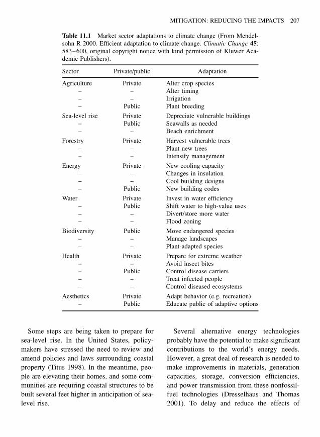
MITIGATION: REDUCING THE IMPACTS 207
Table 11.1 Market sector adaptations to climate change (From Mendel-sohn R 2000. Efficient adaptation to climate change. Climatic Change 45:583–600, original copyright notice with kind permission of Kluwer Aca-demic Publishers).
Sector Private/public Adaptation
Agriculture Private Alter crop species– – Alter timing– – Irrigation– Public Plant breeding
Sea-level rise Private Depreciate vulnerable buildings– Public Seawalls as needed– – Beach enrichment
Forestry Private Harvest vulnerable trees– – Plant new trees– – Intensify management
Energy Private New cooling capacity– – Changes in insulation– – Cool building designs– Public New building codes
Water Private Invest in water efficiency– Public Shift water to high-value uses– – Divert/store more water– – Flood zoning
Biodiversity Public Move endangered species– – Manage landscapes– – Plant-adapted species
Health Private Prepare for extreme weather– – Avoid insect bites– Public Control disease carriers– – Treat infected people– – Control diseased ecosystems
Aesthetics Private Adapt behavior (e.g. recreation)– Public Educate public of adaptive options
Some steps are being taken to prepare forsea-level rise. In the United States, policy-makers have stressed the need to review andamend policies and laws surrounding coastalproperty (Titus 1998). In the meantime, peo-ple are elevating their homes, and some com-munities are requiring coastal structures to bebuilt several feet higher in anticipation of sea-level rise.
Several alternative energy technologiesprobably have the potential to make significantcontributions to the world’s energy needs.However, a great deal of research is needed tomake improvements in materials, generationcapacities, storage, conversion efficiencies,and power transmission from these nonfossil-fuel technologies (Dresselhaus and Thomas2001). To delay and reduce the effects of
208 CLIMATE CHANGE
greenhouse warming, research and technologydevelopment efforts should match, or exceedin scale, previous efforts such as the Man-hattan Project to develop the atomic bomb orthe Apollo Project to land human beings onthe Moon.
Individually, each person must take respon-sibility for his or her own contribution toglobal climate change. Small incrementalchanges, based on individual choices, can addup to substantial change. Individuals shouldconsider, whenever possible, choosing a fuel-efficient car, reducing automobile use, mak-ing their home more energy-efficient, plantingtrees, recycling, and reducing consumption.Individuals have a responsibility to learn moreabout climate change and educate others. Indemocratic nations, individuals should insistthat political candidates reveal their views onclimate change and its mitigation and choosethose candidates who are well informed.
Specifically, individuals can
• turn off electric lights and appliances whennot in use;
• set home and workplace thermostats lowerat night or when gone and higher when airconditioning is used;
• turn water heaters down when gone for aperiod of time;
• set refrigerators no lower than 5 ◦C (41 ◦F)and check the door gasket;
• unplug idle electric appliances;
• replace incandescent light bulbs withenergy-efficient fluorescents;
• wash full loads of clothes and dishes usingcold-water rinse and preferably after 8 pmor during other off-peak hours;
• use a microwave rather than a conventionaloven when possible;
• install improved insulation and seals inyour home;
• walk, bicycle, carpool, or use mass transitwhen possible instead of a single passen-ger vehicle;
• select an energy-efficient automobile andcombine tasks to reduce the number oftrips;
• encourage others to adopt energy-savingpractices.
The exact impacts of climate change arenot, and may not be, totally predictable. Sowhy take mitigative actions that may beexpensive in the face of uncertainty? Thereare several reasons that argue in favor of act-ing sooner rather than later. First, althoughexact effects are not predictable and could insome instances be minimal, it is also true thatsuch uncertainty means that effects could bevery serious or even catastrophic. Second, wehave already committed the Earth to signif-icant climate change; the longer we wait tosubstantially reduce GHG emissions, the moreserious, difficult, and expensive that changewill be. Third, many of the suggested mitiga-tive measures, such as increased energy effi-ciency, will have positive environmental (e.g.improved air quality) and economic benefits.Finally, we have a responsibility to future gen-erations to hand over the planet with a climatethat can sustain the quality of life that we our-selves have experienced, rather than a planetwith a serious problem requiring huge coststo repair.
Summary
Reducing the negative impacts of human-induced climate change on natural ecosystemsand humans represents the greatest environ-mental challenge of this century. At leastfive courses of action could potentially slow
MITIGATION: REDUCING THE IMPACTS 209
the rate of greenhouse warming. All are cur-rently the subject of extensive research bygovernment institutions and private industries.Capturing or sequestering the carbon diox-ide from fossil-fuel combustion at the sourceis technically feasible, at least for station-ary sources, but currently represents a signif-icant added cost for manufacturing or powergeneration. Some large-scale geoengineeringproposals to reduce warming or deal withits effects may be worth further research.However, many are unproven, probably veryexpensive, and probably carry high risks ofenvironmental damage. Natural carbon sinks,for example forests, can be enhanced toabsorb more anthropogenic CO2 emissions.However, reforestation is needed on a hugescale to significantly offset growing carbonemissions. New carbon-free and renewableenergy technologies could each contribute ashare of our growing energy needs whilecontributing little or nothing to atmosphericCO2 levels. Research will continue to improvethe potential of these sources, while reduc-ing their costs. Energy conservation andincreasing energy efficiency, represented byactions of government agencies, industries,and individuals, currently represent the leastexpensive “supply” of carbon-emission-freeenergy. However, efficiency increases alonewill not provide enough energy to sustaincurrent levels of economic growth. Substan-tially meaningful reductions in total globalGHG emissions and stabilization of atmo-spheric CO2 can only be achieved by a con-certed worldwide effort combining differentmitigation approaches.
References
AWEA 2002 American Wind Energy Association .122C Street NW, Washington, DC 2001. Availablefrom: http://www.awea.org.
Begley S 1991 On the wings of Icarus. NewsweekMay: 64,65.
Botkin DB 1989 Can we plant enough trees to absorball the greenhouse gases? Paper presented at theUniversity of California Workshop on EnergyPolicies to Address Global Warming, September6–8, Davis, California.
Boyd PW, Watson AJ, Law CS, Abraham ER,Truli T, Murdoch R, et al. 2000 A mesoscale phy-toplankton bloom in the polar Southern Oceanstimulated by iron fertilization. Nature 407: 695–702.
BTI 2000 Breakthrough Technologies Institute/FuelCells 2000. The Online Fuel Cell Informa-tion Center. Accessed September 9, 2002, from:http://www.fuelcells.org/.
Burns LD, McCormick JB and Borroni-Bird CE2002 Vehicle of change. Scientific American Octo-ber: 64–73.
Chisholm SW, Falkowski PG and Cullen JJ 2001Dis-crediting ocean fertilization. Science 294:309–310.
CO2 Capture Project 2002 An International EffortFunded by Nine of the World’s Leading EnergyCompanies. Accessed September 7, 2002, from:http://www.co2captureproject.org.
David J 2000 Economic Evaluation of LeadingTechnology Options for Sequestration of Car-bon Dioxide [Masters Thesis]. Cambridge: Mas-sachusetts Institute of Technology. Available from:http://sequestration.mit.edu/bibliography/.
Dresselhaus MS and Thomas IL 2001 Alternativeenergy technologies. Nature 414: 332–337.
EC 2002 Atlas Data of Information. The FourthFramework Programme for Research and Techno-logical Development. The European Commission.Accessed September 7, 2002 from: http://europa.eu.int/comm/energy transport/atlas/homeu.html.
Falnes L and Lovseth J 1991 Ocean wave energy.Energy Policy 19(8): 768–775.
Fulkerson W, Reister DB, Perry AM, Crane AT,Kash DE and Auerbach SI 1989 Global warming:an energy technology R&D challenge. Science246: 868–869.
Herzog HJ 2001 What future for carbon captureand sequestration? Environmental Science andTechnology 35(7): 148–153.
IEA 2002 International Energy Agency. Availablefrom: www.ieagreen.org.uk.
Johnson KS and Karl DM 2002 Is ocean fertilizationcredible or creditable? Science 296: 467, 468.
210 CLIMATE CHANGE
Kachadorian J 1997 The Passive Solar House.White River Junction, Vermont, USA: ChelseaGreen Publishing Company.
Keith DW 2001 Geoengineering. Nature 409: 420.Lovins AB and Lovins LH 2002 Mobilizing energy
solutions. The American Prospect 13(2): 18–21.MacLean H, Heather L and Lave LB 1999 Envi-
ronmental implications of alternative-fueled auto-mobiles: air quality and greenhouse gas trade-offs. Environmental Science and Technology 34:225–231.
Mendelsohn R 2000 Efficient adaptation to climatechange. Climatic Change 45: 583–600.
Monastersky R 1995 Iron versus the greenhouse:oceanographers cautiously explore a global warm-ing therapy. Science News 148: 220–222.
Lenton TM and Cannell MGR 2002 Mitigating therate and extent of global warming: an editorialessay. Climatic Change 52: 255–262.
Nakic′enovic′ N 1993 CO2 mitigation: measures andoptions. Environmental Science and Technology27(10): 1986–1989.
NCPV 2002 National Center for Photovoltaics. U.S.Department of Energy, Washington DC. AccessedSeptember 7. from: http://www.nrel.gov/ncpv/.
Newman WS and Fairbridge RW 1986 The manage-ment of sea-level rise. Nature 320: 319–321.
NREL 2002 National Renewable Energy Labo-ratory. U.S. Department of Energy, Washing-ton, DC. Accessed September 7, 2002 from:http://www.nrel.gov.
Ogden JM 1999 Prospects for building a hydrogenenergy infrastructure. Annual Review of Energy andthe Environment 24: 227–279.
Rubin ES, Cooper RN, Frosch RA, Lee TH, Mar-land G, Rosenfeld AH, et al., 1992 Realistic mit-igation options for global warming. Science 257:148, 149, 261–266.
Schneider SH 2001 Earth systems engineering andmanagement. Science 409: 417–421.
Schon JH, Kloc C, Bucher E and Batlogg B 2000Efficient organic photovoltaic diodes based ondoped pentacene. Nature 403: 408–410.
Stultz SC and Kitto JB, eds 1992 Steam: Its Gen-eration and Use. (40th Edition). New York, NY:Babcock and Wilcox Company, Barberton, Ohio,pp. 24-1–24-13.
Titus JG 1998 Rising seas, coastal erosion, and thetakings clause: how to save wetlands and beacheswithout hurting property owners. Maryland LawReview 57: 1279–1399.
U.S. DOE 2002a U.S. Department of Energy, Officeof Science, Carbon Sequestration Program, Wash-ington, DC. Available from: http://cdiac2.esd.ornl.gov.
U.S. DOE 2002b U.S. Department of Energy BiofuelsProgram, Washington, DC. Accessed September 7,2002b from: http://www.ott.doe.gov/biofuels/.
U.S. DOE 2002c U.S. Department of Energy, Wash-ington, DC. http://www.energy.gov/sources/index.html.
U.S. EPA 2000 Average Annual Emissions and FuelConsumption for Passenger Cars and Light Trucks.Air and Radiation, Office of Transportation and AirQuality. EPA420-F-00-013.
World Bank 2002 World Development Indicators2001. Available from: http://www.worldbank.org.
Chapter 12
Policy, Politics,and Economicsof Climate Change
“The economy is a wholly-owned subsidiary of the environment.”
Timothy Wirth, Former US Senator
“We discredit the White House claim that protectingthe climate will harm the economy.”
Heidi Wills, Chair of the City Council Energy and Environmental Policy Committee,Seattle, Washington, February 21, 2002
Introduction
Humans are altering the Earth’s climate. Theproblem is global. The greenhouse emissionsof one country impact all countries. The solu-tion to such a global problem can only comethrough international cooperation. Coopera-tive efforts to solve the problem are underway. However, modern economies depend onfossil-fuel energy, and reducing this depen-dence and greenhouse gas (GHG) emissionsis likely to take considerable time. Also, pol-icy makers, even if they agree on the severityof the problem, often disagree on the bestapproach to solve the problem.
The science of climate change, like allscience, contains some degree of uncertainty.
Conclusions are always subject to modificationas new information is discovered. However,most climate scientists agree that if recent ratesof GHG emissions continue, the result will bewidespread serious damage to ecosystems andhuman enterprises.
In the face of uncertainty, many policy-makers, as well as scientists and individuals,advocate the precautionary principle. Thus,they argue, reducing GHG emissions involvessome costs, but it will also produce benefits.Assuming worst-case climate change predic-tions, reducing GHG emissions now is aninsurance policy against a possible globalenvironmental catastrophe. Taking action nowwill be less costly than waiting until later.
Climate Change: Causes, Effects, and Solutions John T. Hardy 2003 John Wiley & Sons, Ltd ISBNs: 0-470-85018-3 (HB); 0-470-85019-1 (PB)
211
212 CLIMATE CHANGE
To achieve GHG emission reductions, gov-ernments have formulated national policiesand signed international agreements. Almost100 countries have agreed to an internationaltreaty – the 1997 Kyoto Protocol – to reduceGHG emissions and lessen the rate of cli-mate change. However, some argue that sci-ence has not yet proven beyond a doubt thatclimate change will result in significant dam-age to ecosystems or economies. They believethat reducing fossil-fuel use will place toolarge a burden on industry and the economy.
Thus, the climate-change debate has movedinto the political and policy arena. The eco-nomic costs and benefits of different pol-icy options are an active ongoing area ofresearch and debate by opposing groups. Onthe one hand, most conservation groups andsome scientists, economists, and politicians,through reports, presentations, and lobbyingactively, promote policies to mitigate climatechange. On the other hand, many fossil fueland energy trade groups and a few scientists,economists, and politicians argue for unre-stricted fossil-fuel emissions or policies ofminimal climate-change action.
Meanwhile, one thing remains clear –unless the largest contributing countriessharply reduce their emissions, atmosphericGHG concentrations will continue to increaserapidly. The consequences of not achieving aglobal agreement to reduce GHG emissions,although not certain, are likely to be costly.
International Cooperation – FromMontreal to Kyoto
Climate change is a global problem and canonly be solved through international cooper-ation (Luterbacher and Sprinz 2001). Interna-tional cooperative efforts to study the Earth’sclimate have grown since the founding ofthe International Meteorological Organization(IMO) in 1873, culminating in international
agreements to mitigate anthropogenic climatechange (Table 12.1).
The 1987 Montreal Protocol regardingstratospheric ozone depletion by chloroflu-orocarbons was a landmark in internationalgovernmental cooperation on the environment(UNEP 2001). For the first time, countriesfrom around the world approved an inter-national agreement on environmental protec-tion. They agreed to reduce the productionand consumption of 96 chemicals (mostlychlorofluorocarbons and halons) that depletethe stratospheric ozone layer and lead toincreases in damaging ultraviolet radiation.One hundred and eighty countries have rat-ified the Montreal Protocol, but ratificationof subsequent amendments that accelerate thechlorofluorocarbon phase-out with strongercontrol measures lag far behind. The agree-ment significantly reduced the rate of ozonedepletion and avoided tens of millions ofcases of human cancer that would have other-wise resulted from increased ultraviolet radi-ation (UNEP 2001). Perhaps as important,the Protocol provided an example of effec-tive international cooperation to solve a globalenvironmental problem. This example wouldsubsequently be applied in addressing globalgreenhouse warming. In particular, Montrealdemonstrated the usefulness of the “precau-tionary principle,” that is, waiting for com-plete scientific proof can delay action to thepoint at which damage is irreversible.
June 1992 marked an important first stepin international efforts to address climatechange. One hundred and ninety six coun-tries met at Rio de Janeiro, Brazil and throughnegotiation agreed on a “Framework Conven-tion on Climate Change” (UNFCCC 2003).The goal of the convention was to “stabilizegreenhouse gas concentrations in the atmo-sphere at a level that will prevent a dangerousanthropogenic interference with the climate
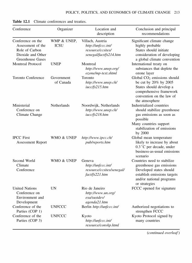
POLICY, POLITICS, AND ECONOMICS OF CLIMATE CHANGE 213
Table 12.1 Climate conferences and treaties.
Conference Organizer Location anddescription
Conclusion and principalrecommendations
Conference on theAssessment of theRole of CarbonDioxide and OtherGreenhouse Gases
WMP & UNEP,ICSU
Villach, Austriahttp://unfccc.int/resource/ccsites/senegal/fact/fs214.htm
Significant climate changehighly probableStates should initiateconsideration of developinga global climate convention
Montreal Protocol UNEP Montrealhttp://www.unep.org/ozone/mp-text.shtml
International treaty onsubstances that deplete theozone layer
Toronto Conference Governmentof Canada
Torontohttp://www.unep.ch/iucc/fs215.htm
Global CO2 emissions shouldbe cut by 20% by 2005States should develop acomprehensive frameworkconvention on the law ofthe atmosphere
MinisterialConference onClimate Change
Netherlands Noordwijk, Netherlandshttp://www.unep.ch/iucc/fs218.htm
Industrialized countriesshould stabilize greenhousegas emissions as soon aspossible
Many countries supportstabilization of emissionsby 2000
IPCC FirstAssessment Report
WMO & UNEP http://www.ipcc.ch/pub/reports.htm
Global mean temperaturelikely to increase by about0.3 ◦C per decade, underbusiness-as-usual emissionsscenario
Second WorldClimateConference
WMO & UNEP Genevahttp://unfccc.int/resource/ccsites/senegal/fact/fs221.htm
Countries need to stabilizegreenhouse gas emissionsDeveloped states shouldestablish emissions targetsand/or national programsor strategies
United NationsConference onEnvironment andDevelopment
UN Rio de Janeirohttp://www.un.org/esa/sustdev/agenda21.htm
FCCC opened for signature
Conference of theParties (COP 1)
UNFCCC Berlin http://unfccc.int/ Authorized negotiations tostrengthen FCCC
Conference of theParties (COP 3)
UNFCCC Kyotohttp://unfccc.int/resource/convkp.html
Kyoto Protocol signed bymany countries
(continued overleaf )
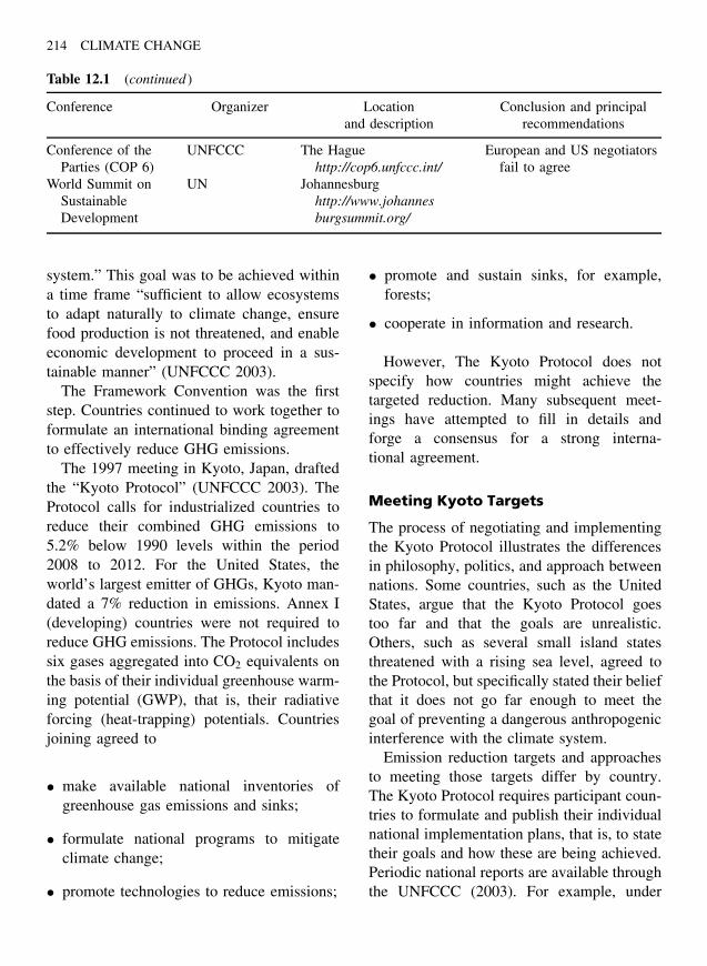
214 CLIMATE CHANGE
Table 12.1 (continued )
Conference Organizer Locationand description
Conclusion and principalrecommendations
Conference of theParties (COP 6)
UNFCCC The Haguehttp://cop6.unfccc.int/
European and US negotiatorsfail to agree
World Summit onSustainableDevelopment
UN Johannesburghttp://www.johannesburgsummit.org/
system.” This goal was to be achieved withina time frame “sufficient to allow ecosystemsto adapt naturally to climate change, ensurefood production is not threatened, and enableeconomic development to proceed in a sus-tainable manner” (UNFCCC 2003).
The Framework Convention was the firststep. Countries continued to work together toformulate an international binding agreementto effectively reduce GHG emissions.
The 1997 meeting in Kyoto, Japan, draftedthe “Kyoto Protocol” (UNFCCC 2003). TheProtocol calls for industrialized countries toreduce their combined GHG emissions to5.2% below 1990 levels within the period2008 to 2012. For the United States, theworld’s largest emitter of GHGs, Kyoto man-dated a 7% reduction in emissions. Annex I(developing) countries were not required toreduce GHG emissions. The Protocol includessix gases aggregated into CO2 equivalents onthe basis of their individual greenhouse warm-ing potential (GWP), that is, their radiativeforcing (heat-trapping) potentials. Countriesjoining agreed to
• make available national inventories ofgreenhouse gas emissions and sinks;
• formulate national programs to mitigateclimate change;
• promote technologies to reduce emissions;
• promote and sustain sinks, for example,forests;
• cooperate in information and research.
However, The Kyoto Protocol does notspecify how countries might achieve thetargeted reduction. Many subsequent meet-ings have attempted to fill in details andforge a consensus for a strong interna-tional agreement.
Meeting Kyoto Targets
The process of negotiating and implementingthe Kyoto Protocol illustrates the differencesin philosophy, politics, and approach betweennations. Some countries, such as the UnitedStates, argue that the Kyoto Protocol goestoo far and that the goals are unrealistic.Others, such as several small island statesthreatened with a rising sea level, agreed tothe Protocol, but specifically stated their beliefthat it does not go far enough to meet thegoal of preventing a dangerous anthropogenicinterference with the climate system.
Emission reduction targets and approachesto meeting those targets differ by country.The Kyoto Protocol requires participant coun-tries to formulate and publish their individualnational implementation plans, that is, to statetheir goals and how these are being achieved.Periodic national reports are available throughthe UNFCCC (2003). For example, under
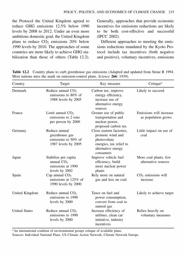
POLICY, POLITICS, AND ECONOMICS OF CLIMATE CHANGE 215
the Protocol the United Kingdom agreed toreduce GHG emissions 12.5% below 1990levels by 2008 to 2012. Under an even moreambitious domestic goal, the United Kingdomplans to reduce CO2 emissions 20% below1990 levels by 2010. The approaches of somecountries are more likely to achieve GHG sta-bilization than those of others (Table 12.2).
Generally, approaches that provide economicincentives for emissions reductions are likelyto be both cost-effective and successful(IPCC 2002).
Different approaches to meeting the emis-sions reductions mandated by the Kyoto Pro-tocol include tax incentives (both negativeand positive), voluntary incentives, emissions
Table 12.2 Country plans to curb greenhouse gas emissions (Adapted and updated from Stone R 1994.Most nations miss the mark on emission-control plans. Science 266: 1939).
Country Target Key measure Critiquea
Denmark Reduce annual CO2
emissions to 80% of1988 levels by 2005
Carbon tax, improveenergy efficiency,increase use ofalternative energysources
Likely to succeed
France Limit annual CO2
emissions to 2 tonsper person by 2000
Greater use of publictransportation andnuclear power,proposed carbon tax
Emissions will increaseas population grows
Germany Reduce annualgreenhouse gasemissions to 50% of1987 levels by 2005
Close eastern factories,promote wind andphotovoltaicenergies, tax relief toalternative energyconsumers
Little impact on use ofcoal
Japan Stabilize per capitaannual CO2
emissions at 1990levels by 2002
Improve vehicle fuelefficiency, buildmore nuclear powerplants
More coal plants, fewalternative sources
Spain Cap annual CO2
emissions at 125% of1990 levels by 2000
Rely more on naturalgas and less on coal
CO2 emissions willincrease
United Kingdom Reduce annual CO2
emissions to 1990levels by 2000
Taxes on fuel andpower consumption,convert from coal tonatural gas
Likely to achieve target
United States Reduce annual CO2
emissions to 1990levels by 2000
Increase efficiency ofutilities, clean carinitiative, industryincentives
Relies heavily onvoluntary measures
aAn international coalition of environmental groups critique of available plans.Sources: Individual National Plans, US Climate Action Network, Climate Network Europe.
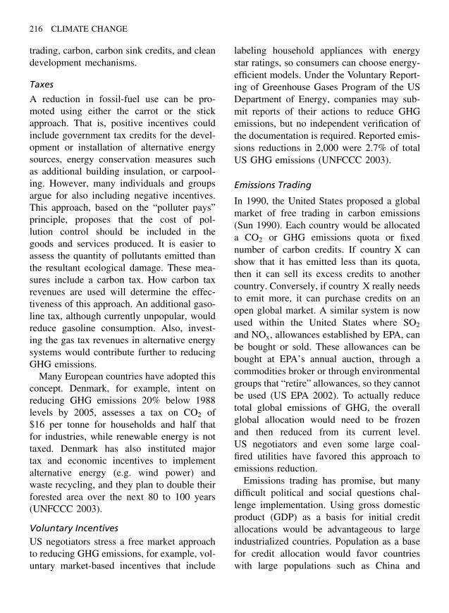
216 CLIMATE CHANGE
trading, carbon, carbon sink credits, and cleandevelopment mechanisms.
Taxes
A reduction in fossil-fuel use can be pro-moted using either the carrot or the stickapproach. That is, positive incentives couldinclude government tax credits for the devel-opment or installation of alternative energysources, energy conservation measures suchas additional building insulation, or carpool-ing. However, many individuals and groupsargue for also including negative incentives.This approach, based on the “polluter pays”principle, proposes that the cost of pol-lution control should be included in thegoods and services produced. It is easier toassess the quantity of pollutants emitted thanthe resultant ecological damage. These mea-sures include a carbon tax. How carbon taxrevenues are used will determine the effec-tiveness of this approach. An additional gaso-line tax, although currently unpopular, wouldreduce gasoline consumption. Also, invest-ing the gas tax revenues in alternative energysystems would contribute further to reducingGHG emissions.
Many European countries have adopted thisconcept. Denmark, for example, intent onreducing GHG emissions 20% below 1988levels by 2005, assesses a tax on CO2 of$16 per tonne for households and half thatfor industries, while renewable energy is nottaxed. Denmark has also instituted majortax and economic incentives to implementalternative energy (e.g. wind power) andwaste recycling, and they plan to double theirforested area over the next 80 to 100 years(UNFCCC 2003).
Voluntary IncentivesUS negotiators stress a free market approachto reducing GHG emissions, for example, vol-untary market-based incentives that include
labeling household appliances with energystar ratings, so consumers can choose energy-efficient models. Under the Voluntary Report-ing of Greenhouse Gases Program of the USDepartment of Energy, companies may sub-mit reports of their actions to reduce GHGemissions, but no independent verification ofthe documentation is required. Reported emis-sions reductions in 2,000 were 2.7% of totalUS GHG emissions (UNFCCC 2003).
Emissions Trading
In 1990, the United States proposed a globalmarket of free trading in carbon emissions(Sun 1990). Each country would be allocateda CO2 or GHG emissions quota or fixednumber of carbon credits. If country X canshow that it has emitted less than its quota,then it can sell its excess credits to anothercountry. Conversely, if country X really needsto emit more, it can purchase credits on anopen global market. A similar system is nowused within the United States where SO2
and NOx, allowances established by EPA, canbe bought or sold. These allowances can bebought at EPA’s annual auction, through acommodities broker or through environmentalgroups that “retire” allowances, so they cannotbe used (US EPA 2002). To actually reducetotal global emissions of GHG, the overallglobal allocation would need to be frozenand then reduced from its current level.US negotiators and even some large coal-fired utilities have favored this approach toemissions reduction.
Emissions trading has promise, but manydifficult political and social questions chal-lenge implementation. Using gross domesticproduct (GDP) as a basis for initial creditallocations would be advantageous to largeindustrialized countries. Population as a basefor credit allocation would favor countrieswith large populations such as China and
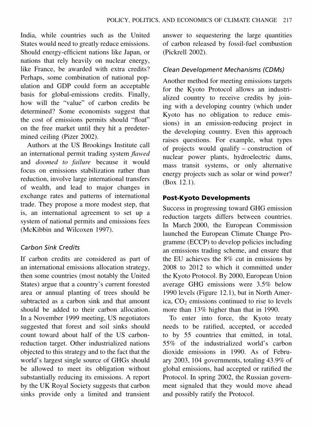
POLICY, POLITICS, AND ECONOMICS OF CLIMATE CHANGE 217
India, while countries such as the UnitedStates would need to greatly reduce emissions.Should energy-efficient nations like Japan, ornations that rely heavily on nuclear energy,like France, be awarded with extra credits?Perhaps, some combination of national pop-ulation and GDP could form an acceptablebasis for global-emissions credits. Finally,how will the “value” of carbon credits bedetermined? Some economists suggest thatthe cost of emissions permits should “float”on the free market until they hit a predeter-mined ceiling (Pizer 2002).
Authors at the US Brookings Institute callan international permit trading system flawedand doomed to failure because it wouldfocus on emissions stabilization rather thanreduction, involve large international transfersof wealth, and lead to major changes inexchange rates and patterns of internationaltrade. They propose a more modest step, thatis, an international agreement to set up asystem of national permits and emissions fees(McKibbin and Wilcoxen 1997).
Carbon Sink Credits
If carbon credits are considered as part ofan international emissions allocation strategy,then some countries (most notably the UnitedStates) argue that a country’s current forestedarea or annual planting of trees should besubtracted as a carbon sink and that amountshould be added to their carbon allocation.In a November 1999 meeting, US negotiatorssuggested that forest and soil sinks shouldcount toward about half of the US carbon-reduction target. Other industrialized nationsobjected to this strategy and to the fact that theworld’s largest single source of GHGs shouldbe allowed to meet its obligation withoutsubstantially reducing its emissions. A reportby the UK Royal Society suggests that carbonsinks provide only a limited and transient
answer to sequestering the large quantitiesof carbon released by fossil-fuel combustion(Pickrell 2002).
Clean Development Mechanisms (CDMs)
Another method for meeting emissions targetsfor the Kyoto Protocol allows an industri-alized country to receive credits by join-ing with a developing country (which underKyoto has no obligation to reduce emis-sions) in an emission-reducing project inthe developing country. Even this approachraises questions. For example, what typesof projects would qualify – construction ofnuclear power plants, hydroelectric dams,mass transit systems, or only alternativeenergy projects such as solar or wind power?(Box 12.1).
Post-Kyoto Developments
Success in progressing toward GHG emissionreduction targets differs between countries.In March 2000, the European Commissionlaunched the European Climate Change Pro-gramme (ECCP) to develop policies includingan emissions trading scheme, and ensure thatthe EU achieves the 8% cut in emissions by2008 to 2012 to which it committed underthe Kyoto Protocol. By 2000, European Unionaverage GHG emissions were 3.5% below1990 levels (Figure 12.1), but in North Amer-ica, CO2 emissions continued to rise to levelsmore than 13% higher than that in 1990.
To enter into force, the Kyoto treatyneeds to be ratified, accepted, or accededto by 55 countries that emitted, in total,55% of the industrialized world’s carbondioxide emissions in 1990. As of Febru-ary 2003, 104 governments, totaling 43.9% ofglobal emissions, had accepted or ratified theProtocol. In spring 2002, the Russian govern-ment signaled that they would move aheadand possibly ratify the Protocol.

218 CLIMATE CHANGE
Box 12.1 Get a higher return on your investments in sustainable energy and energyefficiency
Senter International, an agency of the Netherlands Ministry of Economic Affairs, helpscompanies investing in renewable energy and energy efficiency in developing countries or inCentral and Eastern Europe improve the return on their investments. The Dutch governmentbuys the reduction in greenhouse gas emissions (carbon credits) that these projects generate,thus creating an additional source of income to boost the economic feasibility of projectsand accelerate their implementation (Carboncredits.nl 2002).
Spain
Ireland
Portugal
Belgium
Austria
Denmark
Greece
Italy
Netherlands 5.6
7.2
8.7
8.8
9.2
10.0
16.6
17.5
26.2
France −1.7
Sweden −3.9
Finland −4.1
United Kingdom −6.3
Germany −8.6
Luxembourg
EU-15
−40.0 −30.0 −20.0 −10.0 0.0
DTI
10.0 20.0 30.0
−31.1
0.5
Fig. 12.1 In 2000, total EU greenhouse gas emissions were 3.5% below their 1990 level. Thedistance-to-target indicator (DTI)1 is a measure of the deviation of actual greenhouse gas emissions in2,000 from the linear target path between 1990 and the Kyoto Protocol target for 2008 to 2012,assuming that only domestic measures will be used (From EEA 2002. European Environment Agency.http://www.eea.eu.int/).
The United States initially signed the treaty,but later President George W. Bush announcedthat the US administration would neithersupport ratification of the Kyoto Protocol
1 The Danish DTI is 0.7 index points if Danish greenhousegas emissions are adjusted for electricity trade in 1990.This methodology is used by Denmark to monitor progresstoward its national target under the EU “burden sharing”agreement. For the EU emissions, total nonadjusted Danishdata have been used.
nor enforce emission reduction measures inthe United States. This policy apparentlystems from concerns about negative economicimpacts due to costs of emissions reductions.The United States also objected to the factthat mandatory reductions were limited toindustrialized nations and that developingcountries would not need to meet Protocolemission reduction targets. President GeorgeW. Bush called for more research to reduce

POLICY, POLITICS, AND ECONOMICS OF CLIMATE CHANGE 219
the uncertainties about global warming. Inresponse, the National Academies of Scienceof 17 countries reaffirmed the science alreadyconducted by the IPCC. They stated that, “Thebalance of the scientific evidence demandseffective steps now to avert damaging changesto Earth’s climate” (Science 2002).
In Bonn in July 2001, 180 governmentsagreed to revisions of the Kyoto rules.Revised mechanisms for implementationincluded emissions trading and limitedallowances for carbon sinks such as forests(Giles 2001). However, environmental groupsargued that, by subtracting carbon sinks fromemissions allowances, targets are effectivelyreduced from the 5.2% of the 1990 levelagreed on at Kyoto to something more like1.8% (WWF 2002).
Also, in Bonn, the European Union placedclimate change among its top environmentalpriorities, and established the ECCP to imple-ment policies to meet the goals of Kyoto (EU2002). Several cooperative European effortsare under way. For example, the EuropeanAutomobile Manufacturers Association hascommitted itself to reducing CO2 emissionsfrom automobiles 25% by 2008. Studies bythe European Union estimate that their costof meeting Protocol emission reduction goalswould be reduced 25 to 30% by adoption of aregional EU-wide emissions trading scheme.The EU intends to implement a cap-and-tradesystem covering 46% of all CO2 emissions in2010 (EU 2002).
On August 1, 2001, the US Senate Com-mittee on Foreign Relations voted 19 to 0in favor of US participation in future cli-mate negotiations. The committee stated thatthe United States should not abandon “. . . itsshared responsibility to help find a solution tothe global climate change dilemma.” Perhapsin response, on February 14, 2002, President
Bush announced a new climate-change strat-egy that would set a voluntary “greenhousegas intensity” target for the United States.The greenhouse gas intensity is the ratio ofgreenhouse gas emissions (GHG) to economicoutput (GDP). This ratio has already beendecreasing for decades as energy efficiencyimproves (see Chapter 11). However, eventhough this ratio is decreasing, because ofeconomic and population growth, total GHGemissions continue to rise.
Some have called this US strategy ineffec-tive “. . . blowing smoke,” and emphasizedthat, at the very least, any effective reportingscheme must be mandatory (The Economist2002) (Figure 12.2). The US administration’starget of an 18% reduction in energy intensitybetween 2002 and 2012 will actually allowtotal emissions to increase 12% over the sameperiod – about the same as usual. Current pro-jections of GHG emissions for the UnitedStates indicate an increase of 39% (or withintensity improvements about 33%) over 1990levels by 2012 (EU 2002).
On June 11, 2002, President GeorgeW. Bush spoke about global climate changeand hinted at a more active role for the UnitedStates in solving the climate-change problem.He noted that the recent warming trend was“due in large part to human activity.”
In May 2002, the European Commissionand its 15 member nations ratified the KyotoProtocol. This raised the total number ofparticipating countries to 69 and met thefirst requirement for the treaty to becomeinternational law, that is, ratification by atleast 55 countries. However, ratification byadditional countries will be needed to meetthe second criteria – inclusion of countriesemitting 55% of the global 1990 emissions.As of February 2003, countries representingan additional 11.1% of 1990 emissions wereneeded. The 55% goal could be met through
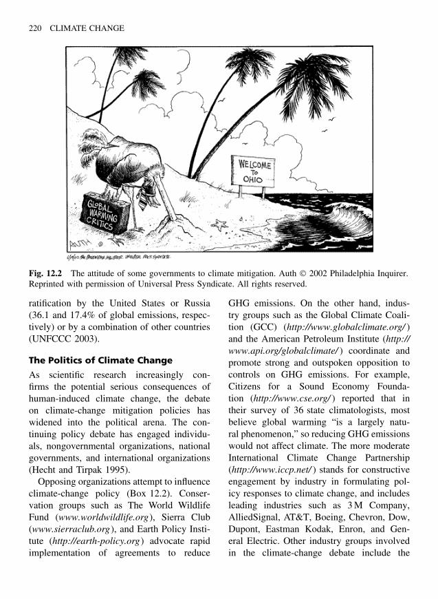
220 CLIMATE CHANGE
Fig. 12.2 The attitude of some governments to climate mitigation. Auth 2002 Philadelphia Inquirer.Reprinted with permission of Universal Press Syndicate. All rights reserved.
ratification by the United States or Russia(36.1 and 17.4% of global emissions, respec-tively) or by a combination of other countries(UNFCCC 2003).
The Politics of Climate Change
As scientific research increasingly con-firms the potential serious consequences ofhuman-induced climate change, the debateon climate-change mitigation policies haswidened into the political arena. The con-tinuing policy debate has engaged individu-als, nongovernmental organizations, nationalgovernments, and international organizations(Hecht and Tirpak 1995).
Opposing organizations attempt to influenceclimate-change policy (Box 12.2). Conser-vation groups such as The World WildlifeFund (www.worldwildlife.org), Sierra Club(www.sierraclub.org), and Earth Policy Insti-tute (http://earth-policy.org) advocate rapidimplementation of agreements to reduce
GHG emissions. On the other hand, indus-try groups such as the Global Climate Coali-tion (GCC) (http://www.globalclimate.org/ )and the American Petroleum Institute (http://www.api.org/globalclimate/ ) coordinate andpromote strong and outspoken opposition tocontrols on GHG emissions. For example,Citizens for a Sound Economy Founda-tion (http://www.cse.org/ ) reported that intheir survey of 36 state climatologists, mostbelieve global warming “is a largely natu-ral phenomenon,” so reducing GHG emissionswould not affect climate. The more moderateInternational Climate Change Partnership(http://www.iccp.net/ ) stands for constructiveengagement by industry in formulating pol-icy responses to climate change, and includesleading industries such as 3 M Company,AlliedSignal, AT&T, Boeing, Chevron, Dow,Dupont, Eastman Kodak, Enron, and Gen-eral Electric. Other industry groups involvedin the climate-change debate include the
POLICY, POLITICS, AND ECONOMICS OF CLIMATE CHANGE 221
Box 12.2 Opposing views
The following excerpts are from the websites of two nongovernmental organizations.
The Global Climate Coalition
“. . . the coalition. . . opposed Senate ratification of the Kyoto Protocol that would assignsuch stringent targets. . . that economic growth in the US would be severely hampered andenergy prices for consumers would skyrocket. The GCC also opposed the treaty because itdoes not require the largest developing countries to make cuts in their emissions.”
World Wildlife Fund
“Climate change and global warming. . . threaten the survival of nature and the well-beingof people around the world. . . reducing CO2 emissions . . . can help prevent unnecessaryloss of life, reduce human suffering and economic disruption from global warming and saveplants and animals from being wiped out over huge areas in the future.”
World Business Council for SustainableDevelopment (http://www.wbcsd.ch/ ) and theBusiness Council for Sustainable Energy(http://www.bcse.org/ ) that promote environ-mentally responsible development and cleanenergy technologies. All groups, through pub-lications and talks, attempt to influence energyand climate-change policy.
Kyoto Without the United States
US politics surrounding the climate-changeissue represent a tug-of-war between thosewho fear potential economic damage fromrestrictions on fossil-fuel combustion andthose who fear for the health of the planetand the longer-term economic consequencesresulting from climate change. Policies haveswung from one pole to another witheach new US administration (Box 12.3). InMarch 2001, US President George W. Bushannounced that the US administration wouldnot support ratification of the Kyoto Protocoland on June 11, 2001, he called the treaty“fatally flawed.” “No one can say forcertainty what constitutes a dangerous level
of warming, and therefore what level mustbe avoided.” He also attacked the agreementfor not including developing countries, likeChina, the world’s second-largest source ofgreenhouse gases. Thus, Protocol participantswere left with two options: (1) adjust theProtocol to meet US objections, that is, forcedeveloping nations to also reduce emissionsor (2) ratify the Protocol without the UnitedStates. Some European groups point to thehuge investment in intellectual and researcheffort that has gone into achieving the KyotoProtocol. Renegotiating a new agreementwould not necessarily improve the agreementand would delay implementation for years.
In a July 2001 survey of four Europeancountries, 80% of respondents agreed thatEuropean governments should begin makingGHG emission cuts in line with the KyotoProtocol whether the United States doesor not (WWF 2002). An analysis of theeconomic implications of unilateral Europeanratification suggests several things (Harmelinket al. 2002). First, without emissions trading,different countries would experience a 0.3 to
222 CLIMATE CHANGE
Box 12.3 History of US climate and energy policy
Climate change is a global problem. However, as the world’s largest single emitter ofgreenhouse gases (GHGs), the policies and politics surrounding this issue in the UnitedStates are particularly critical. In the post-WW II era, US energy consumption exploded. By1973, energy consumption was growing three times faster than the population. Autos weregetting 10% less gas mileage than in 1961 and refrigerators used five times more energythan in the 1940s.
Then, in 1973, one event sparked an abrupt halt to this energy binge. The Organizationof Petroleum Exporting Counties (OPEC) reduced oil production. Because of the high rateof consumption in the United States, shortages quickly developed, resulting in long linesat auto gasoline stations. Some in the US Congress suggested that a major commitment toalternative energy development and energy conservation would need to be undertaken. Thescope of this commitment would need to match that of the Manhattan Project (to developthe atom bomb in WW II) or the Apollo Project (to land a human on the Moon). Thefederal government (Carter administration) instituted major energy conservation measures,including tax benefits for upgrading residential insulation, installation of solar water heaters,wind power generators, and so on. However, by 1980, with oil supplies again abundant, theReagan Administration put any idea of energy conservation on hold. By the mid 1980s, allalternative energy sources together added up to less than 3% of US energy needs. As onepolitician stated, the entire alternative energy budget “. . . is not enough to buy a boosterrocket on the space shuttle.”
In 1987, the US Congress approved, and President Ronald Reagan signed the US ClimateProtection Act (PL 100–204). This law directed the EPA and the Department of State toprepare a report describing the scientific understanding of climate change and the policyoptions for dealing with it. This legislation recognized the importance of protecting theEarth’s climate from human-induced change. Unfortunately, it fell far short of any actualactions or regulations that might mitigate such change.
1988 was a critical year in the politics of climate change. In response to a severe droughtin Central North America and high summer temperatures almost everywhere, many peoplebegan to ask the question – is a radical shift in climate actually under way? The wholeissue of human-induced climate change was thrown into the forefront of public debate.US Senator Timothy Wirth called the greenhouse effect “the most significant economic,political, environmental and human problem facing the 21st Century.” Senator Albert Gorestudied the climate issue, traveled to the Antarctic to observe ozone depletion research andspoke at meetings and conferences on climate change.
During the Presidential candidate debates and the campaign leading up to the election of1988, candidate George Bush (senior) said, if elected, “. . . the greenhouse effect will bematched by the White House effect.” In July 1988, 16 senators unveiled a comprehensiveplan to combat global warming. It would have forced reductions in CO2 emissions of 20%by the year 2000 and required the administration to draft a national energy plan emphasizingways to reduce fossil-fuel use. The bill authorized $1 billion through 1992 for research and
POLICY, POLITICS, AND ECONOMICS OF CLIMATE CHANGE 223
development on solar energy and safer nuclear reactors. It also authorized $1.5 billion toprovide birth control information internationally, but Congress defeated the bill.
Even individual state governments began a flurry of climate-related research andlegislation. For example, the 1988 Washington State Legislature held workshops and heardexpert testimony on climate change. On February 2, 1989, the state approved a resolutionadvising the US Congress to support research on climate change.
In 1989, the US Congress held a hearing chaired by Senator Joseph Lieberman on“Responding to the Problem of Global Warming” (CEPW 1989). The committee gatheredinformation and took testimony from experts about the problem of global warming. However,the new Republican administration suggested that much more research was needed beforeany action to stem GHG emissions could be justified. Indeed, through the Department ofEnergy, the Republican Administration requested a 50% reduction in the national energyconservation program – a budget that had already been cut almost 70% from 1980 levels.
By 1990, many in the United States recognized the need to increase detailed research onclimate change. A National Academy of Sciences Panel on Global Change was formed andchaired by former Washington State Governor Daniel Evans. Also, the US Global ChangeResearch Program was formed to coordinate research among 10 federal agencies. Overall,US funding for research on climate change has grown substantially since 1990. By fiscalyear 2001–2002, this program had a budget of $1.64 billion to study climate change, almosta tenfold increase since 1989–1990 (USGCRP 2002).
However, in terms of energy consumption, little has changed in the past few decades;refrigerators use 600 kWh year−1 when 300 kWh year−1 is possible and the United Stateslags far behind Japan and Europe in energy efficiency. Automobiles achieve an average10 km L−1 (24 mpg) of gas when 30 km L−1 (70 mpg) is possible.
The new administration of George W. Bush, in May 2001, announced a new US energyplan. The plan contained some elements of energy efficiency (e.g. tax credits for alternativeenergy sources and funds for fuel cell research), but emphasized expanding supplies of fossilfuels. Among other things, it recommended that the United States
• study impediments to federal oil and gas exploration and development;
• consider economic incentives for offshore oil and gas development;
• reexamine the current federal, legal, and policy regime regarding siting of energy facilitiesin the coastal zone and Outer Continental Shelf;
• consider oil and gas exploration and development in the Arctic National Wildlife Reserve;
• expedite renewal of the Trans-Alaska Pipeline System rights-of-way;
• invest $2 billion over 10 years in research on coal technology;
• reduce the time and cost of the hydropower licensing process;
• support the expansion of nuclear energy as a major component of our nationalenergy policy.
224 CLIMATE CHANGE
Energy policy has become a hot topic for debate in the United States. Generally, Republicansfavor expansion of fossil-fuel supplies by such measures as opening the Arctic NationalWildlife Refuge to oil drilling, while Democrats favor increasing renewable energy suppliesand increasing auto gasoline efficiency requirements. Republicans charge that Democrats“. . . completely ignored harsh realities in favor of their distant dreams” (Adams 2001).
On March 13, 2002, the US Senate debated raising the Corporate Average Fuel Economy(CAFE) standards for passenger cars from 24 to 36 miles per gallon over a 13-year period. Itwould have been the first increase in standards in 25 years. The Bush administration opposedthe change and the house rejected it.
In contrast to this Republican “supply-side” energy policy, many European and othercountries, as well as some parties in the United States, advocate policies that promoteenergy efficiency and conservation (see Chapter 11). These policies include taxes on fossil-fuel consumption (i.e. a carbon tax), greatly expanding mass transit, conducting large-scalereforestation programs, and providing tax incentives for alternative energy research orinstallation (hydropower, biomass fuel, wind energy, solar energy, fuel cells).
1.9% lower economic growth by 2010 as aresult of implementing the Kyoto ProtocolCO2 reductions. Second, if emissions trading,along with reductions in other GHGs wereconsidered, most industrialized countries willexperience only a 0.1% (or for the UnitedStates about 0.2%) reduction in GDP in2010. Third, the majority of implementationcosts would be compensated for by overallreductions in air pollution control costs, thatis, by reducing CO2 emissions, other airpollutants are reduced at the same time.Finally, the study concluded that 85 to 95%of the reduction target for the EuropeanUnion could be achieved without affecting itseconomic competitiveness. In some scenarios,the European Union, because of increasedenergy efficiency and trade competitiveness,could actually benefit economically from USrejection of the Kyoto Protocol.
A growing number of city and local govern-ments around the world are addressing climatechange. Cities for Climate Protection (CCP)is a campaign of the International Councilfor Local Environmental Initiatives (ICLEI
2002). The CCP offers a framework for localgovernments to develop a strategic agenda toreduce emissions and global warming. Fivehundred local governments, representing 8%of global GHG emissions, are participatingin the Campaign. For example, in the UnitedStates, the Seattle City Council unanimouslypassed a resolution to fully eliminate or mit-igate fossil fuels associated with the City’selectric supply. They also passed a “Kyoto”resolution to inventory all city GHG emis-sions and reduce them, through a variety ofactions, to 7% below 1990 levels, as proposedfor the United States by the Kyoto Protocol.
Benefits and Costs of MitigatingClimate Change
How much we benefit economically frommitigating climate change depends on whatthe costs would be if we do not. However,climate models are somewhat uncertain tobegin with, and when their output is coupledto economic models and regional differences,the uncertainties loom even larger. Thus, thetotal global cost of climate change is not
POLICY, POLITICS, AND ECONOMICS OF CLIMATE CHANGE 225
known. We must rely on individual sector-by-sector (e.g. agriculture, fisheries, etc.) andnational estimates of damage.
One of the direct benefits of implementingan agreement like the Kyoto Protocolis reduced fossil-fuel consumption. Thisalone would have several consequences. Formany industrialized countries, benefits wouldinclude increased energy security resultingfrom a decreased need for oil imports,new business opportunities for companiesproducing alternative energy technologies,and increased energy efficiency and economiccompetitiveness.
The benefits of policies to mitigate climatechange extend beyond direct effects on cli-mate to what are termed ancillary benefits(OECD 2000). These include health, ecolog-ical, economic, and social benefits. If thesebenefits can be given monetary value, theycan then be subtracted from the costs of mit-igation. For example, sulfur dioxide (SO2), acommon air pollutant from fossil-fuel com-bustion, causes acidic rain damage to habitats,and as a lung irritant impacts human health.Therefore, money spent reducing fossil-fuelemissions not only has the benefit of reduc-ing global warming but also of reducing otherair pollutants such as SO2. Economically, thismeans a reduction in SO2 abatement costs aswell as a reduction in health costs related toair quality. In fact, a 15% reduction in CO2
emissions would result in reductions in manyharmful pollutants including ozone, particu-late matter, and SO2 (Figure 12.3).
Another benefit of emissions reductionswill be a decrease in costs for repair-ing the ecological and health damages ofclimate change (Chapters 5–10). An interna-tional insurance agency estimates that morefrequent tropical storms, sea-level rise, anddamage to food and water supplies resultingfrom a doubling of atmospheric CO2 will
cost more than $300 billion per year (MunichRe 2002).
The costs to meet Kyoto emission reduc-tion targets are difficult to estimate. Numerousstudies using computer models that incorpo-rate economic and energy parameters predicta variety of outcomes. Modeling approachesincluding bargaining and game theory (Nash1953) are numerous, complex, and beyondthe scope of this chapter (see Mabey et al.1997). However, many estimated costs forindividual economic sectors have been pub-lished. For example, climate-change mitiga-tion may involve a shift from other fossilfuels to cleaner and more efficient natural gas,requiring tens of thousands of new kilometersof gas pipelines and tripling the cost of elec-tric generation (Anon 2000).
Costs for the United States to meet Kyototargets range from about 0.2 to 4% of GDPper year with typical estimates of about 1to 2.5% of GDP. The GCC, the industrygroup that generally opposes Kyoto, estimatesthat US economic losses from the Protocolby 2010 would range from $120 billion to$440 billion dollars per year. If US growthin GDP continues to grow at rates similarto the past 20 years, this would mean a0.9 to 3.4% decrease in 2010. In otherwords, the GCC estimate of costs agrees withthose of other studies. In the United States,an innovative energy plan, exceeding KyotoProtocol goals by reducing emissions 10%below 1990 levels, could be achieved at a netcost of $530 per household (Alliance to SaveEnergy et al. 1997).
Thus, the costs of meeting Kyoto targetscould be significant. However, the costs of notmeeting the targets may be just as great. Forexample, The American Solar Energy Societyestimates that continued use of fossil fuelswill cost the United States about $100 billion(1989 dollars) a year in environmental and
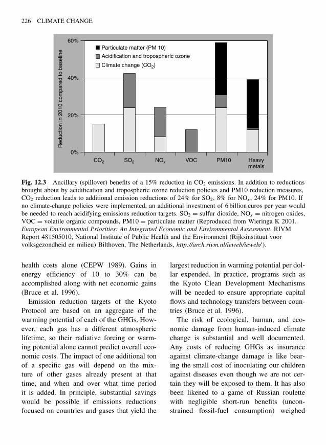
226 CLIMATE CHANGE
60%
40%
20%
0%CO2 SO2 NOx VOC
Red
uctio
n in
201
0 co
mpa
red
to b
asel
ine
PM10 Heavymetals
Particulate matter (PM 10)
Acidification and tropospheric ozone
Climate change (CO2)
Fig. 12.3 Ancillary (spillover) benefits of a 15% reduction in CO2 emissions. In addition to reductionsbrought about by acidification and tropospheric ozone reduction policies and PM10 reduction measures,CO2 reduction leads to additional emission reductions of 24% for SO2, 8% for NOx , 24% for PM10. Ifno climate-change policies were implemented, an additional investment of 6 billion euros per year wouldbe needed to reach acidifying emissions reduction targets. SO2 = sulfur dioxide, NOx = nitrogen oxides,VOC = volatile organic compounds, PM10 = particulate matter (Reproduced from Wieringa K 2001.European Environmental Priorities: An Integrated Economic and Environmental Assessment. RIVMReport 481505010, National Institute of Public Health and the Environment (Rijksinstituut voorvolksgezondheid en milieu) Bilthoven, The Netherlands, http://arch.rivm.nl/ieweb/ieweb/ ).
health costs alone (CEPW 1989). Gains inenergy efficiency of 10 to 30% can beaccomplished along with net economic gains(Bruce et al. 1996).
Emission reduction targets of the KyotoProtocol are based on an aggregate of thewarming potential of each of the GHGs. How-ever, each gas has a different atmosphericlifetime, so their radiative forcing or warm-ing potential alone cannot predict overall eco-nomic costs. The impact of one additional tonof a specific gas will depend on the mix-ture of other gases already present at thattime, and when and over what time periodit is added. In principle, substantial savingswould be possible if emissions reductionsfocused on countries and gases that yield the
largest reduction in warming potential per dol-lar expended. In practice, programs such asthe Kyoto Clean Development Mechanismswill be needed to ensure appropriate capitalflows and technology transfers between coun-tries (Bruce et al. 1996).
The risk of ecological, human, and eco-nomic damage from human-induced climatechange is substantial and well documented.Any costs of reducing GHGs as insuranceagainst climate-change damage is like bear-ing the small cost of inoculating our childrenagainst diseases even though we are not cer-tain they will be exposed to them. It has alsobeen likened to a game of Russian roulettewith negligible short-run benefits (uncon-strained fossil-fuel consumption) weighed
POLICY, POLITICS, AND ECONOMICS OF CLIMATE CHANGE 227
against huge potential losses (from climate-related disasters). “Even worse, the gun ispointed not so much at us as at our children”(DeCanio 1997).
The Future – What is Needed?
Many now consider the Kyoto Protocol onlyas a first step in what may be a negotiatingprocess lasting decades. Even if the Protocolwere fully implemented soon, and industri-alized countries held their emissions at thetargeted levels for the rest of the twenty-firstcentury, GHG concentrations in the atmo-sphere will continue to rise. The time at whichglobal CO2 exceeds twice the preindustriallevel would only be delayed by about a decade(Dooley and Runci 2000). Long-term GHGstabilization will require application of newenergy technologies; yet in many industri-alized countries, investment in publicly andprivately funded energy research and develop-ment is actually declining (Dooley and Runci2000). For example, between 1985 and 1998,the United States, the European Union, andthe United Kingdom collectively reduced theirpublic sector investments in energy R&D by35% in real terms, and US private sectorinvestments fell 53%.
To understand climate change and its effectsrequires large multidisciplinary research pro-grams. Many nations are indeed expandingtheir research efforts to meet the chal-lenge. For example, in the United King-dom, the National Research Councils havecome together to create the multibillion-dollar Tyndall Centre for Climate ChangeResearch. The Centre integrates scientific,social, and technological research and devel-ops sustainable solutions to the societal chal-lenges of climate change. In the UnitedStates, the US Global Change Research Pro-gram, within the Executive Office of Sci-ence and Technology Policy, coordinates
research among federal agencies to provide asound scientific basis for national and inter-national decision making on global changeissues.
Developing countries will contribute anincreasing share of global GHG emissions.For example, China’s contribution to totalglobal carbon emissions is expected to in-crease from 7% in 1990 to 25% in 2020. ForSoutheast Asia, this percentage will increasefrom 7% in 1990 to 25% in 2065. In all,the developing world will account for about75% of future energy growth and most ofthis will come from fossil fuel. This meansthat participation of developing countries ininternational agreements and capacity build-ing in terms of non-fossil-fuel technology iscritical to stabilizing GHGs. Some authorsargue for a century-long plan with a target ofreducing emissions to 50% of their 1990 lev-els by 2100 and thus stabilizing atmosphericCO2 at about 550 ppmv while accommodat-ing significant growth in per capita income(Dooley and Runci 2000). Future agreementsmight include a “graduation” or “ability topay” clause in which non-Annex 1 coun-tries (developing nations) agree that once theireconomy reaches a certain per capita income,they automatically become bound by agreed-on emission reduction targets. By 2100, mostcountries could potentially “graduate” to thiseconomic level (Edmonds and Wise 1999).
In 1997, a group of 2,500 US economists,including 8 Nobel Laureates, signed a publicpronouncement calling for preventative stepsto deal with the threats of global warming(Box 12.4).
Summary
Climate change has emerged as a major polit-ical issue. Some industry groups point tothe uncertainties of climate-change scienceand the economic costs involved in reducing
228 CLIMATE CHANGE
Box 12.4 Statement endorsed by over 2,500 economists including 8 Nobel Laureates
1. The review conducted by a distinguished international panel of scientists under the aus-pices of the Intergovernmental Panel on Climate Change has determined that “the balanceof evidence suggests a discernible human influence on global climate.” As economists,we believe that global climate change carries with it significant environmental, economic,social, and geopolitical risks, and that preventive steps are justified.
2. Economic studies have found that there are many potential policies to reduce greenhousegas emissions for which the total benefits outweigh the total costs. For the United Statesin particular, sound economic analysis shows that there are policy options that wouldslow climate change without harming American living standards, and these measuresmay in fact improve US productivity in the longer run.
3. The most efficient approach to slowing climate change is through market-basedpolicies. In order for the world to achieve its climatic objectives at minimum cost, acooperative approach among nations is required – such as an international emissionstrading agreement. The United States and other nations can most efficiently implementtheir climate policies through market mechanisms, such as carbon taxes or the auctionof emissions permits. The revenues generated from such policies can effectively be usedto reduce the deficit or to lower existing taxes.
The original drafters of this statement are Kenneth Arrow, Stanford University; DaleJorgenson, Harvard University; Paul Krugman, MIT; William Nordhaus, Yale University;and Robert Solow, MIT.
The Nobel Laureate signatories are Kenneth Arrow, Stanford University; GerardDebreu, University of California, Berkeley; John Harsanyi, University of California,Berkeley; Lawrence Klein, University of Pennsylvania; Wassily Leontief, New YorkUniversity; Franco Modigliani, MIT; Robert Solow, MIT; and James Tobin, Yale University.
All signatories endorse this statement as individuals and not on behalf of their institutions.
fossil-fuel consumption. Others, especiallyconservation groups, respected climate scien-tists, and economists, argue that the poten-tially high cost of climate change to ecosys-tems and humans necessitates reduction inGHG emissions now, even in the face ofuncertainty.
The 1992 Framework Convention for Cli-mate Change formed the basis for continu-ing international cooperative efforts to reduceGHG emissions. The subsequent Kyoto Pro-tocol proposes to reduce overall global GHG
emissions below 1990 levels through a vari-ety of mechanisms. It forms the basis forcontinuing negotiations that may eventuallylead to an effective binding internationaltreaty.
Estimates of the costs of mitigating climatechange range from moderately substantial tonegative (i.e. a cost benefit). Predictions thatactions similar to those proposed by the KyotoProtocol will result in economic disaster seemunscientific. In fact, many of the world’s mostnotable economists believe that actions to
POLICY, POLITICS, AND ECONOMICS OF CLIMATE CHANGE 229
reduce GHG emissions will have a long-termnet economic benefit.
References
ACEA 2002 European Automobile ManufacturersAssociation http://www.acea.be/ACEA/index.html.
Adams R 2001 Senate’s Energy Policy Rift Grows asDemocrats Unfurl their Bill and GOP Loses ANWRVote. Congressional Quarterly Dec. 8, p. 2907.Available from: http://www.cq.com.
Alliance to Save Energy, American Council foran Energy-Efficient Economy, Natural ResourcesDefense Council, Tellus Institute, and Union ofConcerned Scientists, 1997 Energy Innovations: AProsperous Path to a Clean Environment. Wash-ington, DC, p. 172, http://www.ase.org/.
Anon 2000 Greenhouse gas reduction news. ElectricPerspectives 25(2): 4–6.
API 2002 American Petroleum Institute Availablefrom: http://www.api.org/globalclimate/.
Bruce JP, Lee H and Haites EF, eds 1996 Cli-mate Change 1995: Economic and Social Dimen-sions of Climate Change. Contribution of Work-ing Group III to the Second Assessment Report ofthe Intergovernmental Panel on Climate Change.Cambridge: Cambridge University Press.
Carboncredits.nl 2002 Senter International, Nether-lands Ministry of Economic Affairs. http://www.senter.nl/asp/page.asp?id=i001003&alias=erupt.
CEPW 1989 Responding to the Problem of GlobalWarming. Committee on Environment and Pub-lic Works, United States Senate. Hearing beforethe Subcommittee on Environmental Protection;August 10. Superintendent of Documents, Wash-ington, DC, p. 122.
DeCanio SJ 1997 The Economics of Climate Change.San Francisco: Redefining Progress. Availablefrom: www.rprogress.org.
Dooley JJ and Runci PJ 2000 Developing nations,energy R&D, and the provision of a planetarypublic good: a long-term strategy for addressingclimate change. Journal of Environment and Devel-opment 9(3): 215–239.
Edmonds J and Wise M 1999 Exploring a technol-ogy strategy for stabilizing atmospheric CO2. In:Carraro C, ed. International Environmental Agree-ments on Climate Change. Boston: Kluwer Aca-demic Publishers, pp. 131–154.
EEA 2002 European Environment Agency, http://www.eea.eu.int/.
EU 2002 European Union, Available from: http://www.europa.eu.int/comm/environment/climat/home en.htm.
Giles J 2001 “Political fix” saves Kyoto deal fromcollapse. Nature 412: 365.
Harmelink M, Phylipsen D, de Jager D and Blok K2002 Kyoto without the U.S.: costs and benefits ofEU ratification of the Kyoto Protocol. ECOFYSEnergy and Environment, Utrecht, The Nether-lands. A report to the World Wildlife Fund. Avail-able from: www.ecofys.com/climate.
Hecht AD and Tirpak D 1995 Framework agreementon climate change: a scientific and policy history.Climatic Change 29: 371–402.
ICLEI 2002 The International Council for LocalEnvironmental Initiatives. Available from: http://www.iclei.org/.
IPCC 2002 Intergovernmental Panel on ClimateChange. United Nations Environment Programmeand World Meteorological Organization, Availablefrom: http://www.ipcc.ch/.
Luterbacher U and Sprinz DF, eds 2001 InternationalRelations and Global Climate Change. Cambridge:MIT Press.
Mabey N, Hall S, Smith C and Gupta S 1997 Argu-ment in the Greenhouse: The International Eco-nomics of Controlling Global Warming . London:Routledge.
McKibbin WJ and Wilcoxen PJ 1997 A Better Way toSlow Global Climate Change. Policy Brief 17, June1997. Washington, DC: The Brookings Institution.Available from: http://www.brook.edu.
Munich Re 2002 Munich Re Group, Munich, Ger-many, Available from: www.munichre.com.
Nash JF 1953 The bargaining problem. Econometrica21: 128–140.
OECD 2000 Ancillary Benefits and Costs of Green-house Gasmitigation. Organization for EconomicCooperation and Development, Proceedings ofan IPCC Co-Sponsored Workshop. 27–29 March,Washington, DC, p. 583, Available from: http://www.oecd.org/env/cc.
Pickrell J 2002 Scientists shower climate change del-egates with paper. Science 293: 200.
Pizer W 2002 Resources for the Future, Availablefrom: http://www.rff.org.
Wieringa K 2001 European Environmental Priori-ties: An Integrated Economic and Environmental
230 CLIMATE CHANGE
Assessment. RIVM Report 481505010, NationalInstitute of Public Health and the Environment(Rijksinstituut voor volksgezondheid en milieu)Bilthoven, The Netherlands, http://arch.rivm.nl/ieweb/ieweb/.
Science 2002 The science of climate change. Edito-rial 292: 1261.
Stone R 1994 Most nations miss the mark onemission-control plans. Science 266: 1939.
Sun M 1990 Emissions trading goes global. Science247: 520–521.
The Economist 2002 United States: blowing smoke.Climate Change 362(8260): 27–28.
UNEP 2001 United Nations Environment Programme.Backgrounder: Basic Facts and Data on the Sci-
ence and Politics of Ozone Protection. http://www.unep.org/ozone/mp-text.shtml.
UNFCCC 2003 United Nations Framework Conven-tion on Climate Change, Available from: http://unfccc.int/.
U.S. EPA 2002 http://www.epa.gov/airmarkets/index.html.
USGCRP 2002 Our Changing Planet: The FY 2002US Global Change Research Program. Report bythe Subcommittee on Global Change Research,Committee on Environment and Natural Resourcesof the National Science and Technology Council,Available from: http://www.usgcrp.gov/.
WWF 2002 World Wildlife Fund. Policy News,Available from: www.worldwildlife.org.
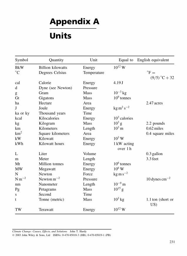
Appendix A
Units
Symbol Quantity Unit Equal to English equivalent
BkW Billion kilowatts Energy 1012 W◦C Degrees Celsius Temperature ◦F =
(9/5)◦C + 32
cal Calorie Energy 4.19 Jd Dyne (see Newton) Pressureg Gram Mass 10−3 kgGt Gigatons Mass 109 tonnesha Hectare Area 2.47 acresJ Joule Energy kg m2 s−2
ka or ky Thousand years Timekcal Kilocalories Energy 103 calorieskg Kilogram Mass 103 g 2.2 poundskm Kilometers Length 103 m 0.62 mileskm2 Square kilometers Area 0.4 square mileskW Kilowatt Energy 103 WkWh Kilowatt hours Energy 1 kW acting
over 1 hL Liter Volume 0.3 gallonm Meter Length 3.3 feetMt Million tonnes Energy 106 tonnesMW Megawatt Energy 106 WN Newton Force kg m s−2
N m−2 Newton m−2 Pressure 10 dynes cm−2
nm Nanometer Length 10−9 mPg Petagrams Mass 1015 gs Second Timet Tonne (metric) Mass 103 kg 1.1 ton (short or
US)TW Terawatt Energy 1012 W
Climate Change: Causes, Effects, and Solutions John T. Hardy 2003 John Wiley & Sons, Ltd ISBNs: 0-470-85018-3 (HB); 0-470-85019-1 (PB)
231

232 CLIMATE CHANGE
Symbol Quantity Unit Equal to English equivalent
µm Micron Length 10−6 mW Watt Power J s−1 = kg m2 s−3
y Year Time

Appendix B
Abbreviations andChemical Symbols
AOGCM Atmosphere-ocean general circulation modelBP Before the present time12C Carbon 12 – most abundant stable isotope14C Carbon 14 – rarer radioactive isotopeCaCO3 Calcium carbonate (limestone)Ca(OH)2 Calcium hydroxide (lime)CFC(s) ChlorofluorocarbonCH4 MethaneCO Carbon monoxideCO2 Carbon dioxide gasDelta �t2x Change in temperature from a doubling of atmospheric CO2
DMS Dimethyl sulfideENSO El Nino Southern OscillationGAT Global average temperatureGCM General circulation (climate) modelGDP Gross domestic productGDPA Gross domestic product agricultureGWP Greenhouse warming potentialHadCM3 Hadley Center for Climate ResearchHCFC(s) HydrochlorofluorocarbonIPCC Intergovernmental Panel on Climate ChangeN2O Nitrous oxideNAO North Atlantic OscillationNOx Nitrogen oxide(s)16O Oxygen – most abundant isotope18O Oxygen – less abundant heavy isotopeO3 OzoneOH− Hydroxyl radicalPFC(s) Perfluorocarbonppb Parts per billion by massppbv Parts per billion by volume
Climate Change: Causes, Effects, and Solutions John T. Hardy 2003 John Wiley & Sons, Ltd ISBNs: 0-470-85018-3 (HB); 0-470-85019-1 (PB)
233

234 CLIMATE CHANGE
pphm Parts per hundred millionppmv Parts per million by volumeRCM Regional climate modelSF6 Sulfur hexafluorideSRES Special Report on Emissions Scenarios by IPCCUNESCO United Nations Education, Scientific, and Cultural OrganizationUNFCCC United Nations Framework Convention on Climate ChangeUV-b Ultraviolet-b radiation (280- to 320-nm wavelength)
Appendix C
Websites onClimate Change
General
US Global Change InformationOffice – Links to a great variety ofinformation on greenhouse warming andclimate change, especially for the UnitedStates. See, for example, “Ask Dr GlobalChange” and your questions will beanswered in a few days.http://www.gcrio.org/
Intergovernmental Panel on Climate Change(IPCC) – The authoritative UN sciencegroup under the auspices of WMO andUNEP. A good site for reviewing currentresearch on climate change. Publicationsand reports are available. See, forexample, full text of “Regional Effects ofClimate Change.”http://www.ipcc.ch/
US EPA Global Climate Website – A goodsource of basic information and references,especially focusing on the United States.http://www.epa.gov/globalwarming/
US Global Change ResearchProgram – Describes agency initiativesand budgets for research and developmentrelated to climate change.http://www.usgcrp.gov/
Energy Information Agency – US DOE linkto many sources of information on bothfossil and nonfossil energy.http://www.eia.doe.gov
European Union – Climate Change Researchand Programs in Europe.http://www.europa.eu.int/comm/enviro-nment/climat/home en.htm
Government of Canada Global ClimateChangehttp://www.climatechange.gc.ca/english/actions/action−fund/index.shtml
Natural Resources Canadahttp://climatechange.nrcan.gc.ca/english/index.asp
United Nations Development Fund andGlobal Environment Facility – Descriptionof project funding on climate changeissues.http://www.undp.org/gef/portf/climate.htm
United States Geological Survey(USGS) – Global Climate Changehttp://GeoChange.er.usgs.gov/
Climate Network Europe – Provides manylinks to other climate information sites.http://sme.belgium.eu.net/∼mli10239/links.htm
Climate Change: Causes, Effects, and Solutions John T. Hardy 2003 John Wiley & Sons, Ltd ISBNs: 0-470-85018-3 (HB); 0-470-85019-1 (PB)
235
236 CLIMATE CHANGE
NOAA Global Warming Home Pagehttp://lwf.ncdc.noaa.gov/oa/climate/globalwarming.html
Journal Articles and Literature onClimate Change
NOAA Links to Climate Products andServices on the WWWhttp://www.pmel.noaa.gov/constituents/climate-services.html
Renewable Energy World Magazinehttp://www.jxj.com/magsandj/rew/2001−01/index.html
The New Scientist – Journal web page withbrief articles and links on all aspects ofclimate change.http://www.newscientist.com/hottopics/climate/
Nature The journal Nature – article abstractsand some full-text articles covering thebreadth of science with some on climatechange.http://www.nature.com/nature/
Environmental Science &Technology – Journal of the AmericanChemical Society. On-line abstract andfull-text articles, some dealing withclimate change.http://pubs.acs.org/journals/esthag/index.html
Global Change – Electronic version ofresearch journal with articles on manyaspects of climate change.http://www.globalchange.org/default.htm
Global Change Master Directory – NASASearchable databases on many aspects ofclimate change.http://gcmd.nasa.gov/
Climate Change Education
UNEP Vital Climate Graphicshttp://www.grida.no/climate/vital/index.htm
US Department of Energy Global ChangeEducation – Information on graduatefellowships and undergraduate summerinternships dealing with climate changeresearch.http://www.atmos.anl.gov/GCEP/
NASA Globe website for Earth Imageshttp://viz.globe.gov/viz-bin/home.cgi
Websites by Chapter Subject Area
Section I Climate Change – Past, Present,and Future
Chapter 1 – Earth and the Greenhouse Effect
University of Reading – AtmosphericRadiation and Climatehttp://www.met.rdg.ac.uk/∼radiation/
NOAA Pacific Marine EnvironmentalLaboratory – Atmospheric Chemistryand Global Changehttp://saga.pmel.noaa.gov/atmochem.html
Carbon Dioxide Information and AnalysisCenterhttp://cdiac.esd.ornl.gov/
Chapter 2 – Past Climate Change: LessonsFrom History
Civilization and past effects of climatehttp://www.msnbc.com/news/564306.asp
Chapter 3–Recent Climate Change: TheEarth Responds
Climate Trend – Data for specificlocations worldwide from the IPCCData Centerhttp://www.climatetrend.com/
APPENDIX C: WEBSITES ON CLIMATE CHANGE 237
NASA – Earth Observatoryhttp://earthobservatory.nasa.gov/Study/GlobalWarm1999/
NOAA Data Center – Portal for searchingand downloading climate data of theNational Oceanic and AtmosphericAdministrationhttp://www.epic.noaa.gov/cgi-bin/NOAAServer?stype=HTML3
Chapter 4 – Future Climate Change: TheTwenty-First Century and Beyond
IPCC Data Distribution Center – A sourceof recent research and data on climatechange with links to specific reports andother sites.http://ipcc-ddc.cru.uea.ac.uk/
Climatic Research Unit University of EastAnglia – Information on climate changeand links to other sites.http://www.cru.uea.ac.uk/
NASA Climate Modeling GoddardInstitute for Space Studieshttp://www.giss.nasa.gov/research/modeling/
Hadley Center for Climate PredictionUK – Part of the UK MeteorologicalOffice. This is an excellent site toreview global climate modelpredictions.http://www.met-office.gov.uk/research/hadleycentre/index.html
National Center for Atmospheric Research(USA)http://www.ncar.ucar.edu/ncar/index.html
Population Action International – This siteparticularly highlights the links betweenworld population growth and recent andfuture climate change.http://www.cnie.org/pop/CO2/intro.htm
Section II Ecological Effects of ClimateChange
Climate Change Impact on Species andEcosystems – A bibliographic list ofresearch articles.http://eelink.net/∼asilwildlife/CCWildlife.html
Chapter 5 – Effects on Freshwater Systems
US Geological Survey Website on ClimateChange – Information on USclimate-change research, particularlythat dealing with soils and waterresources.http://GeoChange.er.usgs.gov/
NASA Global Hydrology and ClimateCenterhttp://wwwghcc.msfc.nasa.gov
Chapter 6 – Effects on Terrestrial Systems
US Forest Service – How the distributionof trees will be affected by climatechangehttp://www.fs.fed.us/ne/delaware/4153/global/global.html
Canadian Forest Service Climate ChangeInformationhttp://www.nrcan.gc.ca/cfs-scf/science/resrch/climatechange−e.html
Chapter 7 – Effects on Agriculture
US Department of Agriculture – NRCS,Agriculture, and Climate Changehttp://www.nrcs.usda.gov/technical/land/pubs/ib3text.html
Global Climate Change and AgriculturalProduction – FAO Book edited by F.Bazzaz.http://www.fao.org/docrep/W5183E/W5183E00.htm
238 CLIMATE CHANGE
Two Essays on Climate Change andAgriculture. UN FAO Economic andSocial Development Paperhttp://www.fao.org/DOCREP/003/X8044E/X8044E00.HTM
Chapter 8 – Effects on the MarineEnvironment
US National Oceanic and AtmosphericOrganization – NOAA Office of GlobalProgramshttp://www.ogp.noaa.gov/enso/
Section III Human Dimensions of ClimateChange
Chapter 9 – Effects on Human Infrastructure
Cities for Climate Protectionhttp://www.iclei.org/co2/index.htm
Electric Power Research Institutehttp://www.epri.com/
US Department of Energy – NationalEnergy Policy and other energy-relatedinformation.http://www.energy.gov/
International Energy Agency –Information on world energy suppliesand policies. http://www.iea.org/
Population Action International – This siteparticularly highlights the links betweenworld population growth and climatechangehttp://www.cnie.org/pop/CO2/intro.htm
Chapter 10 – Effects on Human Health
Program of the Health Effects on GlobalClimate Change of Johns HopkinsUniversity – Lists of publications andlinks to information on health effects.http://www.jhu.edu/∼climate/
Health Canada, Climate Change andHealth Office – Information on healtheffects of climate change.http://www.hc-sc.gc.ca/hecs-sesc/hecs/climate/
World Health Organization – Informationon health effects of climate change, listsof reports and conferences,downloadable articles.http://www.who.int/peh/climate/climate−and−health.htm
Chapter 11 – Mitigation: Reducing theImpacts
American Forests – A nonprofitconservation group. This website allowsindividuals to enter information on oftheir own energy consumption andestimate the number of trees that needto be planted to offset their greenhousegas emissions.http://www.americanforests.org/resources/ccc/
US Department of Energy – SustainableDevelopmenthttp://www.sustainable.doe.gov/
Carbon sequestration bibliographyhttp://sequestration.mit.edu/bibliography/
US Department of Energy – Office ofEnergy Efficiency and RenewableEnergyhttp://www.eren.doe.gov/
Canada – Transportation Initiativeshttp://www.ec.gc.ca/press/clim4−b−e.htm
Photovoltaics – US Dept of Energy,National Center for Photovoltaics.Provides information and interactive
APPENDIX C: WEBSITES ON CLIMATE CHANGE 239
models to calculate energy output andcost savings for any selected area of theUnited States.http://www.nrel.gov/ncpv/
European Commission – EnergySite – Contains information onrenewable sources of energy.http://europa.eu.int/comm/energy−transport/atlas/homeu.html
The Online Fuel Cell InformationCenter – Information on all aspects offuel cells as an energy source.http://www.fuelcells.org/
Biofuels – US Department of Energyinformation on biofuel sources andresearch.http://www.ott.doe.gov/biofuels/
Carbon DioxideSequestration – Description of thecarbon dioxide capture project and otheraspects of CO2 sequestration.http://www.co2captureproject.org
Energy Information Agency – Informationon renewable and fossil and alternativefuels. Good links to other sources.http://www.eia.doe.gov
American Wind EnergyAssociation – Great site for informationon wind energy in general and windenergy projects in the United States.http://www.awea.org
Renewable Energy – The US Departmentof Energy’s laboratory for renewableenergy and energy efficiency researchand development.http://www.nrel.gov/
Danish Wind Industry Association – Allabout wind energy.http://www.windpower.org/core.htm
US Department of Energy – Wind EnergyProgramhttp://www.eren.doe.gov/wind/
American Wind Energy Associationhttp://www.awea.org/default.htm
Alternative Fuels Data Center – USDepartment of Energy Website withinformation on a variety of renewableand noncarbon energy technologies andlinks to related sites.http://www.afdc.doe.gov/altfuels.html
Renewables – European Commission siteon energy.http://europa.eu.int/comm/energy−transport/atlas/htmlu/renewables.html
Chapter 12 – Policy, Politics, and Economics
United Nations Framework Convention onClimate Change (UNFCCC) – The sitefor current information on UN andinternational efforts at global treaties toreduce greenhouse gas emissions andclimate-change effects.http://www.unfccc.de/
US Department of State – site for policyaspects of climate change.http://www.state.gov/g/oes/climate/
Resources for the Futurehttp://www.rff.org/books/descriptions/climatechange−anthology.htm
Indiana University – A WelfareEconomics Perspectivehttp://www.spea.indiana.edu/richards/Welfare−Economics/
Ohio State University – Climate Change:Science, Policy, and Economicshttp://ohioline.osu.edu/ae-fact/0003.html
240 CLIMATE CHANGE
Resources for the Future – Weathervane,A Digital Forum on Climate ChangePolicyhttp://www.weathervane.rff.org/
World Summit on SustainableDevelopment Johannesburg 2002http://www.johannesburgsummit.org/
The Pew Center – Climate Policyhttp://www.pewclimate.org/policy/
Climate Action Network Europehttp://www.climnet.org/
Conservation and EnvironmentalAction Groups
World Wildlife Campaign Climate Changehttp://www.panda.org/climate/
Sierra Club www.sierraclub.org
Earth Policy Institutehttp://earth-policy.org
Hot Earth – An environmental actiongroup dedicated to reducing potentialsfor human-induced climate changehttp://environet.policy.net/warming/index.vtml
Greenpeace – Climate Change Campaignhttp://www.greenpeace.org/campaigns/intro?campaign−id=3937
Industry Groups
Global Climate Coalitionhttp://www.globalclimate.org/
American Petroleum Institutehttp://www.api.org/globalclimate/
Citizens for a Sound Economy Foundationhttp://www.cse.org/
International Climate Change Partnershiphttp://www.iccp.net/
World Business Council for SustainableDevelopmenthttp://www.wbcsd.ch/
Business Council for Sustainable Energyhttp://www.bcse.org/
Global Environmental ManagementInitiative – What business and privateindustry is doing related to globalclimate change.http://www.businessandclimate.org/
Index
acclimatization, 174aerosol(s), 19, 62–65agriculture, 117–130, see also economics
adaptations, farmer, 120, 129animal husbandry, 117, 118, 121crop production, 120, 123
global regions, 123, 125–128United States, 121–125
effects of agriculture on climate, 118effects of climate on agriculture, 120management systems, 119pests and diseases, 121
albedo, 7–8change from re-forestation, 112reduction from ice-melting, 33, 62, 93
algae, toxic blooms, 147alkenones, 29amphibians, 50, 112animal populations, see also ecosystems
future of marine, 140–147future of terrestrial, 110–112life cycle changes, 111recent changes in, 49–50wildlife, 165
anomaliestime-series measurement of, 42
Antarctic, see ice, ozone stratosphericdepletion
Arctic, see ice, permafrost, temperatureArrhenius, Svante, 13, 55atmosphere
chemical composition of, 3–5changes in, 62
circulation patterns, 9history of research on, 4structure of, 5
auto, see vehicle
bears polar, 50, 110biodiversity, 109–112biomass
energy, 158, 191–193global vegetation increase change, 64
birds, 50, 112Bush
President George Wclimate policy, 218, 219, 221
President Herbert W, 222
calcium carbonate, see carbonate calciumcar, see vehiclecarbon
black, 19C-14 age dating, 29credits, 217emissions
from deforestation, 108–109from forest fires, 109
forest, future change in, 64global cycle of, 14–15
feedbacks in, 67intensity, 154sequestration of
agriculture, 119ocean fertilization (ironex), 190reforestation, 112, 190–191
soil, 64, 67tax, 216
carbon dioxide (CO2), see also carbonatmospheric
concentration, 11–12lifetime, 12, 17increase, 13, 15, 69
emissionsagriculture, 118automobile, 162
Climate Change: Causes, Effects, and Solutions John T. Hardy 2003 John Wiley & Sons, Ltd ISBNs: 0-470-85018-3 (HB); 0-470-85019-1 (PB)
241
242 INDEX
carbon dioxide (CO2), see also carbon (Continued )country specific, 13–14from deforestation, 65future, 17, 154from vegetation due to warming, 66sources, 13stabilization of, 72total global, 154
fertilization effect, 64, 108, 121, 127global warming potential, 12ocean source and sink, 17, 138–139phytoplankton uptake, 15reservoirs, 14, 66solubility, 15, 140sequestration, see also economics
ocean storage, 188underground storage, 188forests, 108
stabilization, 154–156, 227carbonate(s)
calcium carbonate (CaCO3), 29, 30, 139cement production and co2 release, 13
chlorofluorocarbons (CFCs), 5, 18, 212, see alsoozone depletion
greenhouse warming potential of, 19–20climate, see also climate change
extremes, 159–160 see also economics ofclimate change
drought, 161flooding, 161heat waves, 172, 174and insurance costs, 160methods of determining past, 29–35monsoon, 71regional, 70
prediction, see also modeling climatesolar activity, 62cryosphere changes and, 62hydrosphere changes and, 62uncertainty from human dimension, 67scenario-based, 67
space of major terrestrial biomes, 99, 100, 110climate change, see also economics, modeling
adaptation to, 206–207attribution of, 51air quality, 159anecdotal evidence of, 40definition of, 11electricity supply and demand, 157–159Great Lakes, US, 89industry, 163–167
land use, 159past, 23–37policy debate, 220–221probability of human induced, 51Protection Act of 1987, 222rapid past, see Younger Dryas Eventrecent, 39–54research programs, 227resource depletion, 159risks of, 226transportation, 162water demand, 159
cloudseffect on climate, 62–63recent increase in, 43–45solar energy reflection, 7
coalcontribution to future GHG emissions,
155–156gasification, 188power plants, 188reserves and lifetime, 17sulfur emissions, 63–64technology and US policy, 223
coral reefsbleaching, 49–50, 142, 145calcium carbonate, 144degradation, 146diseases, 145, 147past climate, 30recent changes in, 49–50
Coriolis force, 9–10, 45costs, see economicscrops, see agriculturecryosphere, see ice, polar, snow
desertification, 107, 161diseases,
crops, diseases and pests, 121–122human non vector-borne, 179
cholera, 179toxic algal blooms, 179
human vector-borne, 175–176dengue fever, 177hantavirus, 177lyme disease, 178malaria, 175–177schistosomiasis, 177trypansomiasis, 179
marine, 147drought, see water
INDEX 243
economic(s), 221–227agriculture, 120–123, 127–128costs of climate change:
adaptation, 206, 207avoiding by fossil fuel reductions, 159carbon sequestration and storage, 188climate extremes, 159–160electricity, 157, 159energy efficiency saving, 203, 205ENSO, 137fishing industry, 142Great Lakes, 89human health, 183industry 163–167infrastructure, 161insurance, 160mitigation, 225reforestation, 112, 191road maintenance, 162sea-level rise, 135, 166–167tourism, 165–167
Kytoto Protocol costs and benefits of, 224–226ecosystems, see also, coral reefs, fish, plankton,
forests, lakes, wetlandsfreshwater, 87–88landscape fragmentation, 113marine
intertidal community, 49, 142mangrove forests, 143salt marshes, 143
terrestrial, 50, 99–115, see also forest(s) andvegetation
savanna, 166wildlife, 166
thermal habitat, 87Ekman transport, see ocean currents and
circulationEl Nino southern oscillation (ENSO)
drought, 86economic cost, 137forest fire increase, 109intensification of, 43, 135, 160malaria, 175–176
energy, 154, see also biomass, fuel cells,hydroelectric, nuclear, solar, tidal, wave,wind
alternative, advantages and disadvantages, 201electrical demand, 157cogeneration, 202–203conservation and efficiency, 201–206intensity, 154, 206
ocean thermal energy conversion (OTEC),197–199
production effects on climate, 154renewable technologies, 191research and development expenditures, 227United States
demand, 157policy, 222–224
environmental quality, 158–159estuaries, 145–147
Chesapeake Bay, 145fisheries, 145impacts of climate change on, 145North Atlantic oscillation and, 145oxygen depletion in, 145Thames estuary, 145
evapotranspiration, 78
feedbacks, see also global carbon cycle, albedodeforestation, 65reforestation, 112, 191
fishchange in distribution, 144fisheries yield, 140north Atlantic, 141northeast PacificNorth Sea cod, 141, 142salmon, 88, 141, 143sardine, 142thermal habitat, 87–88, 140–141trout, 87–88water temperature, 140
flood (s)(ing), see waterforaminifera, 29forest(s), see also vegetation
carbon storage, 13, 108economic value of US, 100fires, 103, 109management and conservation, 112past shifts in distribution in northern hemisphere,
102–103future shifts in US, 103–104reforestation, 190–191Great Lakes, 101spruce, 101US western, 103
fossil fuelglobal reserves, consumption, and lifetime, 17
Framework Convention on Climate Change, seeUnited Nations
fuel cells, 196–197
244 INDEX
geoengineering, 188–190glaciers (glacial)
MIS-11 interglacial warming, 36periods and Earth’s orbital configurations,
24–28retreat of, 46–48, 90
global carbon cycle, see carbon global cycleGore, Albert, 223grassland, see vegetationGreat Lakes
forests, 101infrastructure, 89shipping, 162wetlands, 89
greenhouse effect, 3–8greenhouse gases (GHGs), see also carbon dioxide,
chlorofluorocarbons, methane, nitrous oxide,water vapor
link to recent climate change, 51other GHGs, 19post-industrial atmospheric increase in, 17pre-industrial atmospheric concentration, 11spectral absorption of, 5–8characteristics, 3–5
greenhouse gas (GHG) emissionsair pollution, 181agriculture, 118–119developing countries, 227full fuel cycle, 205–206per capita, 203reduction in, 206, 228
benefits of, 159, 181carbon credits, 217clean development mechanisms, 217endorsement by economists, 228European Union, 217–218energy efficiency, 203, 205–206individual, 208taxes and, 216voluntary incentives for, 216
scenarios of future (SRES), 68–69soils and, 32
warming and increase in 66–67stabilization of, 72, 215, 227trading, 216United States, 219
greenhouse warming potential(s) (GWP), 12–13,19–20
and agriculture, 119Greenland, 48, 90, see also ice
habitat, see also ecosystemfragmentation, 113terrestrial alteration, 110–111
heatacclimatization to, 174global distribution, 8–11infrared, 78latent, 8stroke, 172wave, 172
human health, see also diseasesdirect effects of climate change on humans
171–185acclimatization, 174heart disease, 172–173, 180ozone pollution, 179–180skin cancer, 182stroke, 172–173
interactions and secondary effects, 181United Kingdom effects, 182
human populationcarbon dioxide emissions and, 154drought and flooding effects on, 161migration, 162settlement and infrastructure, 153–169
hydroelectric power, 89, 158, 191hydrology, see waterhydroxyl radical (OH−), 17, 19
iceAntarctic, 90cores and past climate, 31–33Greenland, 48lake, 87, 90sea ice, recent decline of, 46–48
industry, 163–167infrared, see heatinsurance industry, 160infrastructures, 161–162Intergovernmental Panel on Climate Change (IPCC)
assessment reports, 213–214urges action, 219
invertebrates, 111–112, 142
Kaya identity, 154Kyoto Protocol
clean development mechanisms, 217, 226developing countries, 214, 221economic costs and benefits of, 224–226effect on future GHG emissions, 227emissions targets of, 214–218European Union, 224
INDEX 245
ratification of, 219–220requirements of, 217United States policy and, 218–221
lake, sea also icebiota, 86–88
La Nina, see also El Nino southern oscillationeconomic cost, 137
latent heat, see heat latentLiberman, Joseph, 223Little Ice Age, 26, 33livestock, 117–118
malaria, see diseases vector bornemarine environment, 131–150. see also sea-level
risemarine mammals, 147Medieval Warm Epoch, 26, 33methane (CH4)
clathrates (solid methane), 32, 66emissions from agriculture, 118–119future change in, 17, 69greenhouse warming potential of, 19–20radiative forcing global, 20recent increases in, 16sources and atmospheric concentration, 17
Milankovich cycle, 4, 25–28, 32, see also glacialperiods
mitigation 187–210costs, see economicsendorsement by physicians, 183individual actions, 208Kyoto Protocol, 206
modelingagriculture, 120atmosphere-ocean general circulation models
(AOGCMs), 60biogeochemical cycles, 60example of climate, 57–58general circulation models (GCMs), 56–60
historical development of, 58–60validation and testing of, 60–61
research centers for climate, 56temperature sensitivity of climate, 58–59uncertainties in climate, 62–67
Montreal Protocol, 4, 18, 212–213, see also ozonestratospheric
nitrogen oxides (NOx), 179nitrous oxide (N2O), 17, 119nuclear energy, 196
oceanbiogeochemistry, 138–140carbon dioxide (CO2)
source and sink, 14, 66, 139storage of CO2, 188
currents and circulation, 11, see also El NinoSouthern Oscillation (ENSO)
oceanic conveyor belt, see thermohaline oceancirculation
Ekman transport, 45North Atlantic Oscillation, 137North Pacific Oscillation, 138recent changes in, 45–46thermohaline ocean circulation, 136, 138upwelling, 45
fertilization, 190hotspots, 145ph, 139
oxygenisotope ratios and past temperatures, 29–30solubility and depletion in water, 87, 139–140
ozonetropospheric (smog, or “bad ozone”), see also
greenhouse gasesincrease from global warming, 158pollution, 19, 179–180
stratospheric (“good ozone”)depletion, 4, 18, 182, 212, see also Montreal
Protocolultraviolet radiation, 212
and skin cancer, 182
permafrostforest fire effects on, 109response to warming, 66increased stream sediment from melting of, 90and infrastructure, 163
phenology of plants and animals, 111–112plankton, 50, 140
CO2 uptakeand ocean fertilization, 190phytoplankton, recent change in, 51photosynthetic carbon fixation (primary
production), 139polar, see ice, permafrost, temperaturepolicy on climate change, 212–220
European Union, 219United States, 219, 222–223
politics of climate change, 220–224conservation groups, 220industry, 220–221opposing views, 221
246 INDEX
pollenpast climate determination using, 33–35and Younger Dryas Event, 36
population(s), see animal populations or humanpopulations
precipitationfuture global increase in, 70, 77–78global average and range, 77recent trends in, 43
radiative forcing, 19–20future changes in, 65
rainfall, see precipitation
scenariosSpecial Report on Emission Scenarios (SRES),
68–69sea-ice, see icesea-level rise, 132–136
costs of, 135, 167determining sea-level, 133
isostatic adjustment, 133prediction uncertainties, 134
impactsbeach erosion, 134, 135densely populated areas, 135economic, 167ecosystems and humans, 134groundwater (saltwater intrusion), 89island states, 134river deltas, 134United States, 135–136
melting glacier and ice cap contribution to,134
mitigation of, 189recent increase in, 48–49thermal expansion of oceans contribution
to, 132seals, 147skiing, see tourismsmog, see ozone troposphericsnow
alpine snowpack, 91water runoff and irrigation, 91–93
recent decline in cover of, 46, 62, 90solar energy, 193, 195–196
photovoltaic, 195solar radiation
past cycles in, 28spectral distribution of, 5, 6
SRES, see scenarios
stratospherecooling, 42depletion, see chlorofluorocarbonsozone, see ozone stratospheric
stream, see also waterhabitats, 88
sulfate aerosols, see aerosols
technology transfer, 201temperature
Arctic warming, 87change in daily range of, 45, 62change in seasonal range of, 62clouds from increase in, 44–45decrease with elevation, 88Europe 40–42, 70–72future increase in, 55, 69, 72groundwater, 87–88ocean increase, 43past natural variation in global, 26–29, 32, 36persistence of future warmer, 71–72recent trends 40–43sensitivity to increased CO2, 59thermal habitat, 86–87
thermohaline ocean circulation, 11, 35, 136, 138tidal energy, 198time-series, see anomaliestourism, 165–167
ecotourism, 165skiing, 165
transpiration, see evapotranspirationtransportation, 162–163
benefits of climate change, 162carbon dioxide (CO2) emissions, 162efficiency, 201electric cars, 201–202fuel efficiency, 162infrastructure costs, 162, 165road maintenance, 162
treepollen and past climate, 33–35rings and past climate, 33–35
tropospheric ozone, see ozone tropospheric
ultraviolet-b (UV-b) radiationand stratospheric ozone depletion, 18smog formation, 19, 179
United Nations Framework Convention on ClimateChange, 154, 212–213, see also KyotoProtocol
INDEX 247
vegetationboreal and alpine, 105climate space, 101effects on climate, 107–108future shifts in US, 101–106grassland and shrubland, 105–107lake, 90life-cycle changes in, 111past migration, 101, 103recent changes in, 50–51Siberia, 105
vehicle(s)electric, 201–202emissions, 162, 188European Union emission target, 219fuel cell, 196US average emissions of, 224
Vostok, see ice cores
warming, see also temperaturepotential(s), see greenhouse warming potentialspersistence of, 71–72
waterbudget, 78drought, 86, 161flooding, 161management, 93–94North American regions, 82–85per capita availability, 81, 93reservoirs, 79soil moisture, 86surface runoff, 79
Great Britain, 80vapor, 5, 11
recent trends in, 43–45variability, 79World Water Assessment Program,
95wave energy, 198, 200–201wetlands, 90wind energy, 191–194
Younger Dryas Event, 34effect on ocean currents, 46
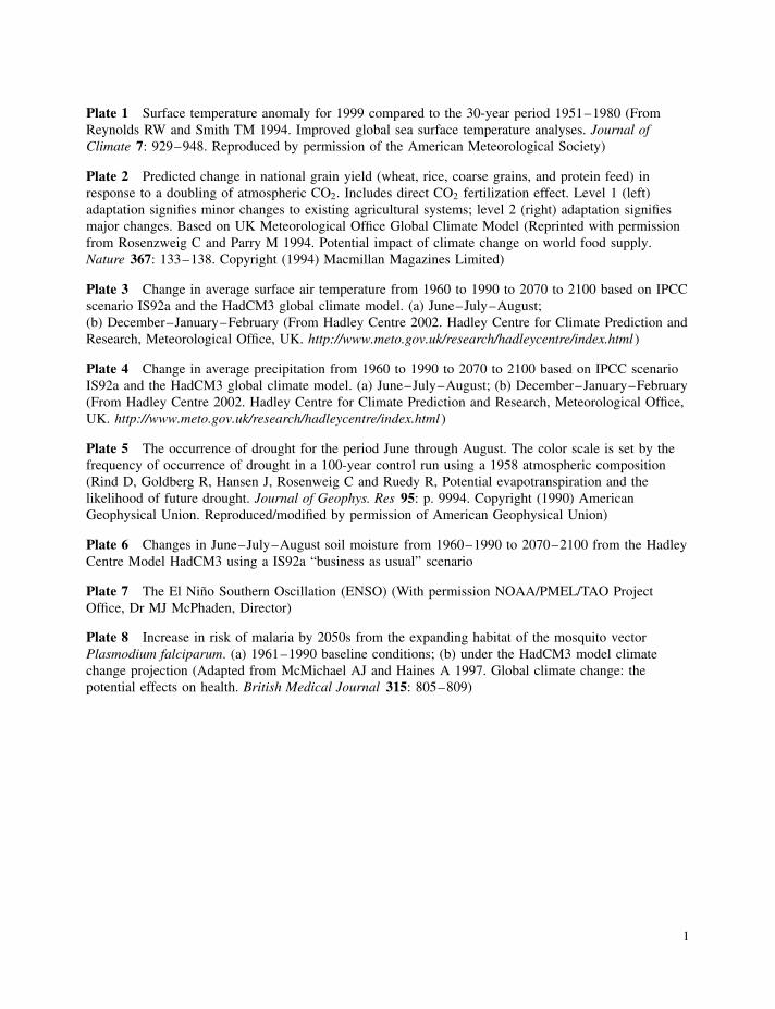
Plate 1 Surface temperature anomaly for 1999 compared to the 30-year period 1951–1980 (FromReynolds RW and Smith TM 1994. Improved global sea surface temperature analyses. Journal ofClimate 7: 929–948. Reproduced by permission of the American Meteorological Society)
Plate 2 Predicted change in national grain yield (wheat, rice, coarse grains, and protein feed) inresponse to a doubling of atmospheric CO2. Includes direct CO2 fertilization effect. Level 1 (left)adaptation signifies minor changes to existing agricultural systems; level 2 (right) adaptation signifiesmajor changes. Based on UK Meteorological Office Global Climate Model (Reprinted with permissionfrom Rosenzweig C and Parry M 1994. Potential impact of climate change on world food supply.Nature 367: 133–138. Copyright (1994) Macmillan Magazines Limited)
Plate 3 Change in average surface air temperature from 1960 to 1990 to 2070 to 2100 based on IPCCscenario IS92a and the HadCM3 global climate model. (a) June–July–August;(b) December–January–February (From Hadley Centre 2002. Hadley Centre for Climate Prediction andResearch, Meteorological Office, UK. http://www.meto.gov.uk/research/hadleycentre/index.html )
Plate 4 Change in average precipitation from 1960 to 1990 to 2070 to 2100 based on IPCC scenarioIS92a and the HadCM3 global climate model. (a) June–July–August; (b) December–January–February(From Hadley Centre 2002. Hadley Centre for Climate Prediction and Research, Meteorological Office,UK. http://www.meto.gov.uk/research/hadleycentre/index.html )
Plate 5 The occurrence of drought for the period June through August. The color scale is set by thefrequency of occurrence of drought in a 100-year control run using a 1958 atmospheric composition(Rind D, Goldberg R, Hansen J, Rosenweig C and Ruedy R, Potential evapotranspiration and thelikelihood of future drought. Journal of Geophys. Res 95: p. 9994. Copyright (1990) AmericanGeophysical Union. Reproduced/modified by permission of American Geophysical Union)
Plate 6 Changes in June–July–August soil moisture from 1960–1990 to 2070–2100 from the HadleyCentre Model HadCM3 using a IS92a “business as usual” scenario
Plate 7 The El Nino Southern Oscillation (ENSO) (With permission NOAA/PMEL/TAO ProjectOffice, Dr MJ McPhaden, Director)
Plate 8 Increase in risk of malaria by 2050s from the expanding habitat of the mosquito vectorPlasmodium falciparum. (a) 1961–1990 baseline conditions; (b) under the HadCM3 model climatechange projection (Adapted from McMichael AJ and Haines A 1997. Global climate change: thepotential effects on health. British Medical Journal 315: 805–809)
1

This Page Intentionally Left Blank

Plate 1MSurface temperature anomaly for 1999 compared to the 30-year period 1951–1980. From NASA EarthObservatory http://earthobservatory.nasa.gov/Study/GlobalWarm1999. (See Chapter 3).
Plate 2MPredicted change in national grain yield (wheat, rice, coarse grains, and protein feed) in response to a doublingof atmospheric CO2. Includes direct CO2 fertilization effect. Level 1 (left) adaptation signifies minor changes to existingagricultural systems; level 2 (right) adaptation signifies major changes. Based on UK Meteorological Office GlobalClimate Model. Reproduced with permission from Rosenzweig C and Parry M 1994, Potential impact of climate changeon world food supply. Nature 367: 133–138. Copyright © 1994 Macmillan Magazines Limited. (See Chapter 7).
–3 –2 –1.5 –1 –0.5 –0.2 0.2 0.5 1 1.5 2 3.0
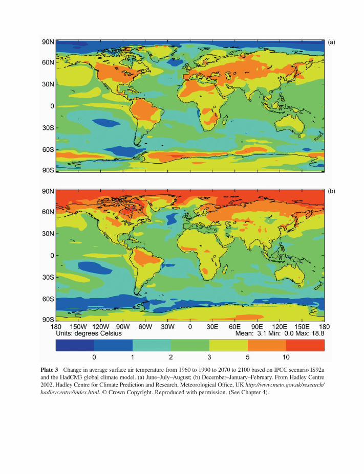
Plate 3MChange in average surface air temperature from 1960 to 1990 to 2070 to 2100 based on IPCC scenario IS92aand the HadCM3 global climate model. (a) June–July–August; (b) December–January–February. From Hadley Centre2002, Hadley Centre for Climate Prediction and Research, Meteorological Office, UK http://www.meto.gov.uk/research/hadleycentre/index.html. © Crown Copyright. Reproduced with permission. (See Chapter 4).
(a)
(b)

Plate 4MChange in average precipitation from 1960 to 1990 to 2070 to 2100 based on IPCC scenario IS92a and theHadCM3 global climate model. (a) June–July–August; (b) December–January–February. From Hadley Centre 2002,Hadley Centre for Climate Prediction and Research, Meteorological Office, UK http://www.meto.gov.uk/research/hadleycentre/index.html. © Crown Copyright. Reproduced with permission. (See Chapter 4).
(a)
(b)
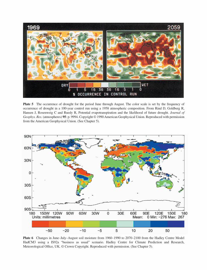
Plate 5MThe occurrence of drought for the period June through August. The color scale is set by the frequency ofoccurrence of drought in a 100-year control run using a 1958 atmospheric composition. From Rind D, Goldberg R,Hansen J, Rosenweig C and Ruedy R, Potential evapotranspiration and the likelihood of future drought. Journal ofGeophys. Res. (atmospheres) 95: p. 9994. Copyright © 1990 American Geophysical Union. Reproduced with permissionfrom the American Geophysical Union. (See Chapter 5).
Plate 6MChanges in June–July–August soil moisture from 1960–1990 to 2070–2100 from the Hadley Centre ModelHadCM3 using a IS92a “business as usual” scenario. Hadley Centre for Climate Prediction and Research,Meteorological Office, UK. © Crown Copyright. Reproduced with permission. (See Chapter 5).
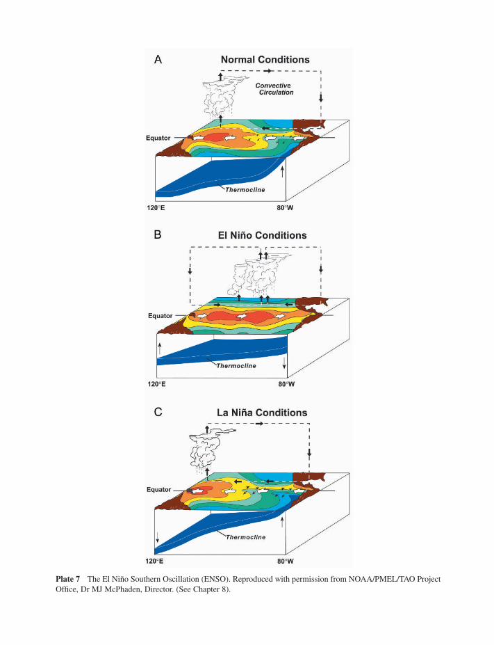
Plate 7MThe El Niño Southern Oscillation (ENSO). Reproduced with permission from NOAA/PMEL/TAO ProjectOffice, Dr MJ McPhaden, Director. (See Chapter 8).
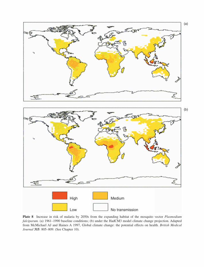
High
Low
Medium
No transmission
Plate 8MIncrease in risk of malaria by 2050s from the expanding habitat of the mosquito vector Plasmodiumfalciparum. (a) 1961–1990 baseline conditions; (b) under the HadCM3 model climate change projection. Adaptedfrom McMichael AJ and Haines A 1997, Global climate change: the potential effects on health. British MedicalJournal 315: 805–809. (See Chapter 10).
(a)
(b)