Climate change awareness:

Empirical evidence for the European Union

Donatella Baiardi and Claudio Morana

No 426/rev

FEBRUARY 2021 

Climate change awareness: Empirical evidence forthe European Union∗

Donatella Baiardi+and Claudio Morana∗†+University of Parma

∗University of Milano-Bicocca∗+Center for European Studies (CefES)

∗+Rimini Centre for Economic Analysis (RCEA)∗Center for Research on Pensions and Welfare Policies (CeRP)

February 2021

Abstract

In this paper, we assess public attitudes on climate change in Europe overthe last decade. Using aggregate figures from the Special Eurobarometer surveyson Climate Change, we find that environmental concern is directly related to percapita income, social trust, secondary education, the physical distress associatedwith hot weather, media coverage, the share of young people in the total popula-tion, and monetary losses caused by extreme weather episodes. It is also inverselyrelated to greenhouse gas emissions, relative power position of right-wing partiesin government and tertiary education. Moreover, we find a significant, oppositeimpact for two dummies for years 2017 and 2019, which we respectively associatewith the effects of Donald Trump’s denial campaigns and the U.S. Paris Agreementwithdrawal announcement, and Greta Thunberg’s environmental activism.Keywords: climate change, environmental attitudes/concern, mitigation policy,

EUJEL classification: Q50, Q54, Q58

∗A previous version of this paper was presented at the International workshop NESPUTT 2019(University of Milano-Bicocca), CREDIT 2020 (University of Venice), the 28th Annual Symposium ofthe Society for Nonlinear Dynamics and Econometrics, the 61th Meeting of the Italian EconomistsAssociation, the 4th International Conference on Computational and Financial Econometrics. We aregrateful to conference participants, P. Natale, N. Cassola, E. Ossola, L. Alessi, and three anonymousreviewers for constructive comments. We are also grateful to S. Walter and L. Tiozzo for help with thedata.†Address for correspondence: Claudio Morana, Università di Milano - Bicocca, Dipartimento di

Economia, Metodi Quantitativi e Strategie di Impresa, Piazza dell’Ateneo Nuovo 1, 20126, Milano,Italy. E-mail: claudio.morana@unimib.it.

1

1 IntroductionWhat are public perceptions of climate change? Initially at low levels in the early 1980s, whenthe issue started to be widely acknowledged in most industrialized countries, public concern forclimate change appears to have converged to consensus levels over the next two decades, as aconsequence of growing scientific evidence and higher mass media coverage and political debate(Nisbet and Myers, 2007; Boykoff and Yulsman, 2013). International consensus on the urgencyof climate change mitigation also appears to have been achieved by mid-2000s. Yet awarenessof the contribution of various human activities to the phenomenon, such as energy use, animalfarming, food miles and waste, does not appear to have risen much over time (Laiserowitz, 2008;Attari et al., 2010; Brechin, 2010; Whitmarsh et al., 2011; Bailey et al., 2014).

The 2015 “Paris Agreement”represents the highest level of worldwide consensus ever achievedsince the Rio Earth Summit in 1992, in relation to the existence of climate change, its human-made origin, and the urgent need to implement mitigation and adaptation policies. Under theagreement, 196 countries committed to the goal of keeping the increase in global average tem-perature well below 2◦C above pre-industrial levels and, in particular, to limit this increase to1.5◦C, in order to reduce the risks and impacts of climate change.

The Paris Agreement was even more remarkable as it followed a period of widespread skep-ticism. This had started in the late 2000s and intensified during Donald Trump’s campaign forthe U.S. Presidency, his election in 2016 and his announcement of U.S. withdrawal from theagreement in June 2017 (Laiserowitz et al., 2014; 2017). Donald Trump, who defined climatechange as a “hoax”, during his U.S. presidency consistently acted against the objectives of theParis Agreement and dismantled many environmental protection measures in the U.S.1

Recent evidence shows that, at current levels of greenhouse gas emissions, the carbon budgetfor meeting the Paris Agreement target of 2◦C will be exhausted in less than three decades,while less than a decade is left to limit the increase in global temperature to 1.5◦C.2 Yet thesescenarios might even be optimistic, since greenhouse gas emissions are still increasing globallyand there might in fact be no time left to avoid large-scale discontinuities in the climate system.It could be that there is no time left to avoid tipping points and that the only remainingpossibility is to limit damage as tipping points are reached: “The stability and resilience of ourplanet is in peril. International action -not just words- must reflect this”(Lenton et al., 2019).

In the light of this evidence, understanding the drivers of climate change attitudes is animportant and urgent task, since in democratic systems the legitimacy of political decisions onclimate change mitigation actions relies on the support of public opinion. This will be in favouronly where there is suffi cient concern for the economic, human and social implications of climatechange. In this paper we focus on the evolution in climate change concern in Europe over thelast decade. The period investigated is interesting, as it allows us to assess how Europeanclimate change attitudes have been affected by the “Paris Agreement”, the election of DonaldTrump as U.S. President, his denial campaigns and the environmentalists’ response led byGreta Thunberg and the “Fridays for future”movement. To the authors’knowledge, there areno studies in the literature focusing on data more recent than 2014. Moreover, our assessmentis based on the Special Eurobarometer surveys on Climate Change, which are in-depth thematic

1See the running list maintained by The National Geographic:https://www.nationalgeographic.com/news/2017/03/how-trump-is-changing-science-environment/.

2According to IPCC (2018), the atmosphere can absorb, calculated from end-2017, no more than 420(1,170) gigatonnes (Gt) of CO2 if it is to stay below the 1.5◦C (2◦C) threshold. Since around 42 Gt ofCO2 is emitted globally every year, i.e. 1,332 tonnes per second, this carbon budget is expected to beused up in about nine (twenty six) years.

2

studies integrated into Standard Eurobarometer’s polling waves and published every two yearssince 2009. Although the Special Eurobarometer surveys provide an accurate view of climatechange attitudes, they have been neglected in the literature so far. Finally, unlike previousstudies, our analysis focuses on aggregate survey results over different countries. This paperthus fills some important gaps in the literature.

We find that, over the last decade, climate change concern in Europe has increased with thelevel of per capita income. We name this relationship “climate change/environmental awarenesscurve”(CCA curve). This curve is theoretically motivated by the public good nature of envi-ronmental quality, for which demand increases with the level of income, and is well describedby a logistic function. This curve is also related to the “environmental Kuznets curve”, whichdescribes an inverse-U shaped relationship between greenhouse gas emissions and the level ofper capita income. Intuitively, once threshold income level is crossed, economic developmentbecomes sustainable, i.e. higher income levels are associated with lower emissions, and, in ourframework, also with higher climate change concern. Significant effects are also found for socialtrust, greenhouse gas emissions, education, the physical distress associated with hot weather,the share of young people in the total population, relative power position of right-wing parties ingovernment, media coverage and economic losses caused by extreme weather episodes. All thesevariables act as shift factors for the climate change awareness curve (in its awareness-incomespace), in some cases also impacting on its slope.

Moreover, we also find a significant impact for two temporal dummies for year 2017 and2019, accounting for a sizable drop and a sizable increase in environmental concern, respectively,ceteris paribus. While our study cannot establish causal linkages, consistent with our theoreticalframework and the available empirical evidence on political leader-follower linkages, in relationto climate change attitudes, we are inclined to associate these changes with Donald Trump’sdenial campaigns and politicization of climate change and Greta Thunberg’s environmentalactivism, respectively. By keeping in mind the above mentioned caveat on causality, in the lightof the estimated effects, the positive Thunberg effect appears to have prevailed over the negativeTrump effect. Climate change concern in the EU would have then risen as a consequence ofpublic controversy brought to the fore by the election of Donald Trump as U.S. President.

The rest of the paper is organized as follows. Section 2 reviews the existing literature onclimate change attitudes in Europe. Section 3 provides some stylized facts about climate changeattitudes for the EU member countries. Section 4 presents the environmental awareness/concerndissemination model and its econometric specification. Section 5 describes the data, Section 6presents the empirical results and Section 7 concludes.

2 Literature reviewPsychology has traditionally identified three components of mind: cognition, affect, and cona-tion. Cognition is the process of rationally understanding a phenomenon, through the acquisi-tion and processing of information. Affect refers to the emotional response to the acquisition ofthis knowledge. Conation refers to the personal, intentional action, i.e. the proactive behavioralresponse caused by the cognitive and affective experiences (Tallon, 1997). The literature on en-vironmental attitudes has explored all three of the above components, i.e. the understanding ofthe climate change phenomenon, the emotions associated with this knowledge and the actionstaken to mitigate its impact and adapt to its effects. Comprehensive surveys by Lorenzoni andPidgeon (2006), Upham et al. (2009) and Whitmarsh and Capstick (2018) provide a broadoverview of the field.

Concerning recent European evidence, Wicker and Beckern (2013) analyze Eurobarometer75.4 survey data, collected in June 2011 from a sample of 26,840 respondents. Survey questionsconcern the perceived severity of climate change, relative to concerns about energy availability

3

and the economic situation, and any personal action taken by respondents to fight climate changeduring the six months before the interview. For instance, questions cover the purchase of newlow fuel consumption cars or new low-energy homes, the consumption of locally produced andseasonal food, and transport habits in relation to alternatives to the use of private cars (walking,bike, public transport, car-sharing). By means of linear regression analysis, they find a positiveimpact of education, wealth and life satisfaction, as well as of concerns about economic, energyavailability and climatic conditions, on respondents’ proactive behavior. Socio-demographicfactors also matter, since women and young people appear to be more active in environmentalprotection than men and old people. The above findings are confirmed by Meyer (2015), usingdata from Eurobarometer 68.2 (November 2007-January 2008) and 75.2 (April-May 2011) andregression discontinuity analysis.

D’Amato et al. (2019) focus on determinants of environmentally-friendly behavior, in rela-tion to waste reduction, waste recycling, water saving and energy saving activities. The datainvestigated are from three Special Eurobarometer surveys on attitudes of European citizenstowards the environment, collected in 2008, 2011 and 2014. By means of a system of simul-taneous linear regressions, they find a positive influence of the level of information, especiallythrough internet sources, the level of trust on organization and scientists, the level of GDP, and,in some cases, the level of mean temperature, environmental expenditure and energy taxation,on environmentally-friendly behavior. However, a negative impact is found for tertiary educa-tion. Drews et al. (2018), using the same survey data, also find that respondents tend to vieweconomic growth and environmental protection as compatible objectives, even prioritizing theenvironment in a trade-off situation.

Poortinga et al. (2018) investigate data collected in Round 8 of the European Social Survey.The sample consists of 44,387 respondents in 23 European countries. The survey covers climatechange beliefs and concerns and environmental policy preferences. The evidence shows thatabout 90% of respondents believe that the climate is changing, partly as a consequence ofhuman activities. Moreover, although 70% of respondents, on average, expect climate changeeffects to be bad or very bad, only 25% state that they are very worried. Consistently with this,the majority of respondents say that it is less than likely that they will undertake mitigationactivities in the near future, for instance in relation to their energy use.

A larger international sample of European and non European countries is considered inFranzen and Vogl (2013) and Smith and Mayer (2018), who use data for 33 countries fromthe International Social Survey Programme (ISSP) on environmental protection, for the years1993, 2000, and 2010, and data for 35 countries from the Life in Transition II Study (LITS II)conducted by the World Bank and the European Bank for Reconstruction and Developmentin 2010, respectively. ISSP data are also employed by Lo and Chow (2015). In particular,Franzen and Vogl (2013) construct an index of environmental concern, accounting for both thecognitive and conative components of climate change attitudes, Smith and Mayer (2018) focuson the determinants of the willingness to act to fight climate change, and Lo and Chow (2015)consider the ranking of climate change in terms of its importance relative to other problemsand the danger associated with it in terms of sense of insecurity and risk. By means of panelregression techniques, Franzen and Vogl (2013) and Smith and Mayer (2018) find a positiveimpact of education, social and institutional trust, GDP or per capita GDP on environmentalattitudes. Moreover, by means of a multilevel logistic regression and using EU27 data, Harring(2014) finds that in relatively more corrupt and economically unequal (Southern European)countries, economic pro-environmental policy instruments (EIs) are considered less effectivethan in relatively less corrupt and economically unequal (Northern European) countries. Thisis consistent with the fact that corrupt public institutions tend to waste economic resources andto have lower levels of trust in public policy. These results are important, as public support forclimate mitigation action is high when the perceived policy effectiveness is also high. Smith and

4

Mayer (2018) also find a positive effect for the perceived gravity of climate change, while Franzenand Vogl (2013) also point to significant impacts of gender, age and political factors. On theother hand, Lo and Chow (2015) document a positive impact of per capita GDP on the relativeranking of climate change across challenges, but negative effects of per capita GDP, energy useand the Global Adaptation Notre-Dame Index (ND-GAIN) on its (absolute) perceived gravity.See also the earlier studies of Diekkman and Franzen (1999), Sandvik (2008) and Freymeyerand Johnson (2010), based on various international survey data on European and non Europeanconsumers’environmental attitudes.

Interesting results are also reported in Frondel et al. (2017) and Andor et al. (2018), basedon survey data collected by the German institute forsa Gesellschaft für Sozialforschung undstatistische Analysen. The survey counts more than 6,000 respondents, representative of thepopulation of German speaking households aged 14 and above. The survey is updated regularlyand available for various years and increasing sample size, i.e. 2012 (6,404 respondents), 2013(6,522 respondents), 2014 (6,602 respondents) and 2015 (7,077 respondents). In particular,Frondel et al. (2017) focus on the association of public perception of climate change withheat waves, storms and floods, and their financial and physical costs. Andor et al. (2018)consider the perceived importance of taking action against climate change. By means of orderedlogit regression estimation, they find that personal experience with adverse natural events,particularly personal losses, lead to higher environmental concern, and that older people arenot likely to personally engage in fighting climate change or supporting policy measures aimingat climate change mitigation. Survey data, based on about 1,000 respondents in Germany only,are also used in Schwirplies (2018). In particular, perceptions of climate change are assessed inrelation to global warming, climate change mitigation policies, i.e. the development of renewableenergy sources and energy-effi cient technologies, and climate change adaptation policies, i.e.the construction of infrastructures to protect against future natural disruptions. By meansof bivariate ordered probit regressions, she finds that support for mitigation and adaptationactions positively correlates with the recognition of the anthropogenic origin of climate change(responsibility factor), the view that these actions can still be effective and political supportfor the green party. On the other hand, a negative linkage is found for the level of income andmixed effects for education.

3 Stylized facts about climate change concern in theEuropean Union

Our proxy variables for climate change concern are based on aggregate country figures, retrievedfrom the Special Eurobarometer surveys on Climate Change, collected every two years, over theperiod 2009-2019. In particular, we consider results contained in Volume C (Country/socio-demographics). The issues investigated are no. 322 (2009), 372 (2011), 409 (2013), 435 (2015),459 (2017) and 490 (2019).3 The sample includes the 27 current EU member countries plus theUK.4 Hence, we provide an up to date assessment of climate change attitudes in Europe, basedon specialized surveys.

More specifically, our analysis focusses on the following questions: “Which of the followingdo you consider to be the single most serious problem facing the world as a whole?”, “Whichothers do you consider to be serious problems?”, “And how serious a problem do you thinkclimate change is at this moment?”. These questions cover the cognitive component of climate

3See, for instance, https://data.europa.eu/euodp/en/data/dataset/S2212_91_3_490_ENG.4Current EU Member States are Austria, Belgium, Bulgaria, Cyprus, Croatia, Czechia, Denmark,

Estonia, Finland, France, Germany, Greece, Hungary, Ireland, Italy, Latvia, Lithuania, Luxembourg,Malta, Netherlands, Poland, Portugal, Romania, Sweden, Slovakia, Slovenia and Spain.

5

change attitudes and, to some extent, its emotional component, assuming that a negative feelingis associated with environmental concern, and the intensity of the feeling is proportional to thedegree of perceived gravity of the environmental problem.

In the first two cases, we use the percentage of respondents that identify climate change asthe single most serious global challenge in each country (QB1a) or that rank climate change thesecond to fourth most serious global challenge (QB1b).5 For the third question, we select thoserespondents who consider climate change as a serious problem (QB2s) and as a very seriousproblem (QB2vs), by assigning scores within ranges 5-6 and 7-10, respectively (in a scale from 1to 10, with “1”meaning it is “not at all a serious problem”and “10”meaning it is “an extremelyserious problem”).

Moreover, we also aggregate the above figures and obtain three additional proxy variables.The aggregation of QB1a and QB1b yields the percentage of respondents who rank climatechange as one of the four most important global challenges (QB1). The aggregation of QB2sand QB2vs yields the percentage of respondents who consider climate change at least a seriousproblem (QB2), giving a score within the range 5-10. The interaction (product) of QB1 andQB2 yields an estimate of the percentage of respondents who rank climate change as one ofthe four most important challenges and at least of serious gravity (QB1QB2).6 All these seriesare used in our study as alternative proxy variables for environmental concern, i.e. yt = QB1a,QB1b, QB2s, QB2vs, QB1, QB2, QB1QB2.

3.1 The empirical evidenceAs shown in Table 1, (on average) 58% of the interviewed EU citizens in 2019 view climatechange as one of the four major global challenges (Panel C), and 22% of them rank it as thebiggest challenge (Panel A). As regards gravity, 16% of respondents view it as a serious problem(Panel D) and 77% of them as a very serious problem (Panel E).

The comparison with earlier Eurobarometer results shows that EU environmental attitudeshave not evolved linearly over time. For instance, (on average) climate change is ranked withinthe first four most important challenges by 50% of the respondents already in 2009 (Panel C).This figure does not alter sizably until 2019 (+6% (12%) relatively to 2009 (2017)), apart fromthe most sizable contraction occurred in 2017 (-7% relatively to 2009). Similarly, 18% of therespondents already rank climate change as the most important threat in 2009 (Panel A). Thisfigure then sizably raises in 2019 (+4% (9%) relative to 2009 (2017)). The perceived gravity ofthe phenomenon shows a steadier pattern, since 63% of the respondents consider climate changeat least a serious problem already in 2009 (Panel F). This figure then increases to about 67%over the three following survey periods, to 72% in 2017 and, eventually, to 77% in 2019. Similarinformation is provided by our overall climate change concern measure QB1QB2 (Panel G). Infact, according to interacted figures, (on average) in 2009 already 45% of respondents regard

5As well as climate change, the other possible responses are: international terrorism, poverty, hungerand lack of drinking water, spread of infectious diseases, the economic situation, proliferation of nuclearweapons, armed conflicts, increasing global population and other items.

6As we can access aggregated figures only, we cannot compute exactly the percentage of respondentswho simultaneously rank climate change as one of the four most important challenges (A) and assigneda score between 5 and 10 to its perceived gravity (B). In terms of probabilities, we have P (A ∩ B) =P (A)× P (B|A), which we estimate as P (A)× P (B). Yet 1) it is very likely that a respondent rankingclimate change as one of the four most important challenges will also consider it a threat of at leastserious gravity, i.e say P (B|A) > 0.9; 2) in our sample P (B) (across countries and time) ranges betweena minimum of 0.7 and a maximum of 0.99, taking a median value equal to 0.91. Then, we can concludethat using P (B) in the place of P (B|A) in our case might yield a satisfactory estimate of the unobservedquantity of interest. With this caveat in mind, in what follows we then simply refer to QB1QB2 as if itwere the actual measure, rather than the estimated measure, of the percentage of respondents who rankclimate change as one of the four most important challenges and at least of serious gravity.

6

climate change as one of the four most important challenges and at least of serious gravity. Asizable drop can then be noted in 2017 and an even more sizable increase in 2019 (+9% (14%)relative to 2009 (2017)).

In Figure 1 we compare cross-sectional distribution patterns in years 2009 and 2019. Den-sity estimation is performed through (Gaussian) kernel smoothing, under optimal bandwidthselection (Silverman, 1986). As shown in Figure 1, distributional dynamics provide additionalinsights on raising climate change concern in the EU over the last decade. For instance, evidenceof emerging polarization or bi-modality can be seen in the distribution of QB1a, consistent withthe formation of a group of (leading) countries for which climate change might have become themost important challenge. The shrinking dispersion in the distribution of QB1b sends a similarmessage. Over time, the perception that climate change is one of the four main important chal-lenges has become more homogeneous across countries. Consistently with this, the distributionof QB1 (sum of QB1a and QB1b) shows a clear-cut rightward shift in 2019 relative to 2009.

Moreover, just as the distribution of respondents seeing climate change as a very seriousproblem shows a rightward shift (QB2vs), the distribution of respondents seeing climate changeas an at least serious problem also shows a similar pattern. This indicates an overall increasein the number of Europeans concerned about the gravity of climate change. The distribution ofthe interacted variable QB1QB2 also shows a rightward shift, which still appears to be bimodalin 2019, yet of shrinking dispersion relative to 2009 figures.

However, as shown by the heat maps reported in Figure 2 for QB1QB2 and in Figure A1(in the Online Appendix) for the other proxy variables, geographical dispersion in attitudesis still sizable even in 2019. In particular, environmental concern appears to be highest forNorthern European countries and lowest for Eastern European countries. For instance, NorthernEuropean countries show the highest percentages of respondents who rank climate change as themost important challenge (Figure A1, Panel A); Western and Southern European countries showthe highest percentages of respondents who rank climate change between the second and fourthmost important challenges (Figure A1, Panel B); Northern and Southern European countriesshow the highest proportion of interviewed that rank climate change as a very serious threat(Figure A1, Panel D). Coherently, the shares of respondents who rank climate change as oneof the four most important challenges (Figure A1, Panel E), a threat of at least serious gravity(Figure A1, Panel F), and one of the four most important challenges, of at least serious gravity(Figure 2), are higher for Northern, Western and Southern European countries than EasternEuropean countries.

The overall conclusion from the above results is that concern for climate change in the EUhas risen over time, but neither in a linear nor a homogeneous manner. Most interesting are thesizable drop in 2017 and the even more sizable raise in 2019. In the light of recent events and thepotential effect of leadership cues on public polarization on environmental issues (Lewis-Becket al., 2011), we are inclined to associate these changes with Donald Trump’s denial campaignsand Greta Thunberg’s environmental activism, which have impacted on climate change atti-tudes worldwide over the last three years. In fact, the drop in concern in 2017 might possiblyreflect Donald Trump’s denial speeches and the U.S. Paris Agreement withdrawal announce-ment in June 2017. Withdrawal was not effective before November 2020, but the announcementalready impacted on the prospects of compliance by raising the cost of emission cuts for compli-ant countries and aggravating the leadership deficit in addressing climate change. Politicizationof climate change by the Trump administration to some extent also jeopardized the authorityof scientific evidence on climate change. On the other hand, the sizable upward shift in EUenvironmental attitudes in 2019 possibly reflects public response to Greta Thunberg’s envi-ronmental activism and the “Fridays for future movement”. Greta Thunberg’s “solo”protest,which started in September 2018, rapidly became a worldwide phenomenon, and involved about4 million people across 169 countries by September 2019. Over the last year, Greta Thunberg

7

has attended various high-profile events across Europe and the U.S., including U.N. climatemeetings. In March 2019 she was nominated for the Nobel Prize, in May 2019 was named oneof the world’s most influential people by the Time magazine and in December 2019 its Personof the Year.

This interpretation appears to be consistent with the very robust evidence on the politicalleader-follower linkage, in relation to climate change perceptions, already available for the U.S.For instance, Dunlap (2014) argues that conservative political leaders in the U.S. contribute todistrust in scientific evidence on climate change and to climate change skepticism among layconservatives. Brulle et al. (2012) and Carmichael and Brulle (2016) also find that Congres-sional attention on climate change, which in turn influences media coverage, is the single mostimportant determinant of public concern in the U.S. In this respect, the impact of elite opinionon mass opinion would be indeed mediated through media coverage. Similar conclusions arealso drawn in Egan and Mullin (2017); see also Björnberg et al. (2017).

4 The climate change awareness curveNonlinearity and the potential role played by opinion leaders, noted in the above descriptiveanalysis, are reminiscent of the “S -shaped” information dissemination model, recently repro-posed by Shiller (2017). This model predicts that an “innovation”, when the decision to adoptis voluntary, will spread among the members of a social system in an S-shaped curve (sigmoidcurve), in a manner similar to infection diseases. In our context, the S -shape, which describesthe evolution of climate change attitudes, is modelled through the following logistic function

y =1

1 + exp (−x′γ) , (1)

where y is a given proxy for climate change concern, x is a vector of socio-demographic, eco-nomic, political and climatological control variables and γ the associated vector of parameters.

Standard theory posits that the S -shape arises from the engagement of opinion leaders, whoactively diffuse the innovation and introduce it to other potential adopters, the characteristics(complexity) of the innovation and the capability of adoption of the social system, which dependson socio-demographic, economic and political characteristics. This dissemination process is alsoconsistent with leader-follower relations grounded on elite cues, whereby leaders influence theirrespective group identifiers by providing ‘cues’that help their followers to shape their beliefson specific issues (Lewis-Beck et al., 2011).

Adoption then proceeds through a multi-stage process of assessment, acceptance and as-similation. It takes time for new ideas and concepts to become widely accepted. The S -curveposits a very slow rate of dissemination for a new idea at its inception. But if the spread of thenew concept persists over time, what is initially accepted by only a few, and possibly ridiculedor even opposed by many, subsequently enters the mainstream and is accepted as self-evidentand given by the majority. This pattern is traditionally grounded in the Kermack-McKendrickmodel of epidemics of disease, but the progressive saturation process is also reminiscent of theearlier, more general view expressed by the German philosopher Arthur Schopenauer (1788-1860), in his important book, The World as Will and Representation: “The truth is alwaysdestined to have only one brief victory parade between two long time spans in which it is firstbeing condemned as paradoxical and then belittled as trivial.”7 This quotation fits the basis ofour theory of climate change attitudes, which can be specified mathematically by a functiondescribing logistic dissemination, conditional to a set of determining variables.

7Der Wahrheit ist allezeit nur ein kurzes Siegesfest beschieden zwischen den beiden langen Zeiträumen,wo sie als paradox und als trivial gering geschätzt wird. [The World as Will and Representation, Prefaceto the First Edition, p. xxv; German: Die Welt als Wille und Vorstellung].

8

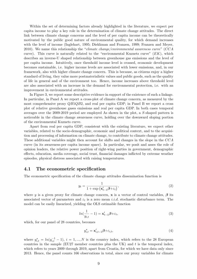
Within the set of determining factors already highlighted in the literature, we expect percapita income to play a key role in the determination of climate change attitudes. The directlink between climate change concerns and the level of per capita income can be theoreticallymotivated by the public good nature of environmental quality, for which demand increaseswith the level of income (Inglehart, 1995; Diekkman and Franzen, 1999; Franzen and Meyer,2010). We name this relationship the “climate change/environmental awareness curve”(CCAcurve). This curve is naturally related to the “environmental Kuznets curve” (EK), whichdescribes an inverse-U shaped relationship between greenhouse gas emissions and the level ofper capita income. Intuitively, once threshold income level is crossed, economic developmentbecomes sustainable, i.e. higher income levels are associated with lower emissions, and, in ourframework, also with higher climate change concern. This is because, as citizens enjoy a higherstandard of living, they value more postmaterialistic values and public goods, such as the qualityof life in general and of the environment too. Hence, income increases above threshold levelare also associated with an increase in the demand for environmental protection, i.e. with animprovement in environmental attitudes.

In Figure 3, we report some descriptive evidence in support of the existence of such a linkage.In particular, in Panel A we report a cross-plot of climate change concern, as measured by themost comprehensive proxy QB1QB2, and real per capita GDP; in Panel B we report a crossplot of relative greenhouse gases emissions and real per capita GDP. In both cases temporalaverages over the 2009-2019 period are employed As shown in the plot, a S -shaped pattern isnoticeable in the climate change awareness curve, holding over the downward sloping portionof the environmental Kuznets curve.

Apart from real per capita GDP, consistent with the existing literature, we expect othervariables, related to the socio-demographic, economic and political context, and to the acquisi-tion and processing of information on climate change, to contribute to climate change attitudes.These additional variables might then account for shifts and changes in the slope in the CCAcurve (in its awareness-per capita income space). In particular, we posit and asses the role ofopinion leaders, the relative power position of right-wing parties in government, demographiceffects, education, media coverage, social trust, financial damages inflicted by extreme weatherepisodes, physical distress associated with raising temperatures.

4.1 The econometric specificationThe econometric specification of the climate change attitudes dissemination function is

yt =1

1 + exp(x′t−1β+εt

) , (2)

where y is a given proxy for climate change concern, x is a vector of control variables, β itsassociated vector of parameters and εt is a zero mean i.i.d. stochastic disturbance term. Themodel can be easily linearized, yielding the OLS estimable function

ln(1

yi,t− 1) = x′t−1β+εt, (3)

which, for our panel of 28 countries, becomes

y∗i,t = x′i,t−1β+εi,t, (4)

where y∗i,t = ln(y−1i,t − 1), i = 1, ..., N is the country index, which refers to the 28 Europeancountries in the sample (EU27 member countries plus the UK) and t is the temporal index,which refers to years 2009 through 2019, apart from Croatia, for which we have data only since2013. Hence, the panel counts 166 observations in total, since our proxy variables for climate

9

change concern are available at a biannual frequency. Moreover, εi,t ∼ i.i.d.(0, σ2ε

). Then,

comparison between (1) and (2) yields γ = −β.The lead-lag model is a natural setting for the investigation of the data at hand, since

survey results are collected in March/April and therefore much earlier than the contemporaneouscontrol variables. Accordingly, all the regressors sampled at an annual frequency enter thespecification with a one year lag. When 2018 figures are missing, as in a few cases, they arereplaced with their 2017 values.

Since the conditioning regressors are predetermined, under poolability conditions, the OLSestimator is expected to provide consistent and asymptotically normal estimates.

Still within the above pooled specification, the panel data nature of our data can be taken intoaccount by the inclusion of some conditioning variables that are either time-invariant (allowingto control for stochastic country-effects) or country-invariant (allowing to control for stochastictime-effects).

Given the large set of potential regressors available, we implement a general to specificspecification strategy, which, through a sequential reduction procedure based on statisticaltesting, yields a final parsimonious econometric model describing the phenomenon of interest.

The specification in (4) can however be augmented to account also for unknown sources ofcross-sectional random effects (in addition to those already controlled for by the inclusion oftime-invariant regressors), yielding

y∗i,t = δi + x′i,t−1β+εi,t, (5)

where εi,t ∼ i.i.d.(0, σ2ε

), δi ∼ i.i.d.

(0, σ2δ

), and εi,t and δi are mutually independent. Moreover,

the regressors are still predetermined, and therefore not contemporaneously correlated with εi,tand δi. Under these conditions the OLS estimator of β is consistent, but delivers distortedstandard errors. Consistent and more accurate estimation can then the performed by means ofthe Estimable Generalized Least Squares Estimator (EGLS).

Since some of the potentially relevant regressors are time-invariant, the alternative fixedeffects approach cannot be implemented using the standard within transformation. Fixed effectscan however be accounted for, also when time-invariant regressors are included in the model,by following a general to specific procedure, implemented through an autometrics/saturationalgorithm (Hendry et al., 2008; Johansen and Nielsen, 2009; Doornik, 2009).8

The specification in (4) can then be augmented to account for deterministic country andtime effects, as well as for influential observations, yielding

y∗i,t = x∗′i,t−1β+

N∑j=1

dji,tδi+T∑s=1

τ stηs +

TN∑j=1s=1

ij,si,t θis + εi,t, (6)

where di,t = 1 if i = j and 0 else (step country-i effect), τ s,t = 1 if s = t and 0 else (year -s effect), ij,si,t = 1 if i = j, s = t and 0 else (impulse country-i at year-s effect), δi, ηs, θisare parameters, and εi,t ∼ i.i.d.

(0, σ2ε

). Since the regressors are predetermined, OLS yields

consistent and asymptotically normal estimation.Deterministic time and country effects are then selected, as for the other conditioning vari-

ables, through an automated general to specific reduction strategy. Hence, relative to standardpanel data modelling, our approach is also likely to yield effi ciency improvements, due to theparsimony ensured by the general to specific estimation strategy. Moreover, in the light of theresults of the descriptive analysis, the saturated regression analysis makes it possible to assess

8The econometric analysis and GETS specification analysis has been performed by meansof the OxMetrics 8 package by D.F. Hendry and J.Doornik. The package is available athttps://www.timberlake.co.uk/software/oxmetrics.html#products.

10

the robustness of our findings to potential sources of model misspecification, such as outliersand structural change. These can be attributed to events gone unaccounted in the model andto shifting distributions, for instance in terms of sudden location shifts and changes in the trendrate of growth, respectively.

Since the selected deterministic country effects are potentially large in our context, effi ciencyand estimation accuracy might be increased by combining the retained deterministic effects ina single variable, as delivered by their linear combination, with weights appropriately selected.This constrained version of model (4) is the restricted or constrained saturated model

y∗i,t = x∗′i,t−1β+αFCEi,t +

T∑s=1

τ stηs + εi,t, (7)

where

FCEi,t =N∑j=1

dji,tw(δi) +

TN∑j=1s=1

ij,si,tw(θis),

and w(δi), w(θis) are the weights employed in the linear combination of fixed country effectsFCEi,t. Upon testing the restrictions implicit in the construction of FCEi,t, the constrainedmodel in (7) can be consistently estimated by OLS. The constrained model grants the same fit,specification and robustness properties of its unconstrained version, yet a higher effi ciency andaccuracy, due to the larger number of degrees of freedom available.

Finally, notice that the transformed dependent variable y∗i,t, by construction, takes valuesin the [−∞,+∞] interval, making our linearized specification in principle compatible with anadditional assumption of conditional Gaussianity for the error term; this would grant to theOLS estimator the usual interpretation in terms of ML estimator, therefore ensuring consistent,asymptotically normal and asymptotically effi cient estimation.

Also, in the empirical implementation, in order to improve numerical accuracy, the non-negative explanatory variables are transformed according to the function

x∗ij,t =xij,t −min(xj)

max(xj)−min(xj),

where x∗ij,t is the country i, time period t panel observation for the generic regressor j; max(xj)and min(xj) are the maximum and minimum values for the generic regressor j over the panelsample, respectively. Thus, by construction, the transformed regressors take values in the [0, 1]interval.

5 The dataThe proxy variables for climate change attitudes are denoted by the variable yt = QB1a, QB1b,QB2s, QB2vs, QB1, QB2, QB1QB2. All these series are already described in Section 2. Onthe other hand, various control variables for the underlying socio-demographic, economic, andpolitical environment and (academic and non-academic) information sources are included in theset of regressors xt in (4).

Firstly, consistent with the direct linkage between environmental attitudes and standard ofliving described by climate change/environmental awareness curve, we include real per capitaGDP (GDP ). The series employed in the study is the chain linked volumes (2010) Euro percapita gross domestic product at market prices, available from Eurostat for each of the countriesin the sample.

Secondly, we posit a role for two opinion leaders, i.e. U.S. President Donald Trump (“brown”leader) and Greta Thunberg (“green” leader), whose activities might be best associated with

11

events occurring in 2017 and 2019, respectively. Hence, two dummy variables are included, i.e.,an impulse time dummy for year 2017 (DT ), to control for the potential impact of Donald Trumpdenial campaigns, dismantling of environmental protection in the U.S. and announcement ofthe U.S. withdrawal from the Paris Agreement in 2017; an impulse time dummy for year 2019(GT ), to control for the potential impact of Greta Thunberg’s environmental activism and the“Fridays for Future”movement, which, started in 2018, became a worldwide phenomenon inearly 2019.

Moreover, a lower environmental concern might be expected in countries ruled by right-wing/conservative parties, which generally represent the interests of business and industries inWestern countries (Franzen and Vogl, 2013; McCright et al., 2016).9 As a measure of Govern-ment political composition, we then include an index of relative power position of right-wingparties in government, based on their share of seats in parliament, measured as a percentage ofthe total parliamentary seat share of all governing parties, weighted by the number of days inoffi ce in a given year (GRP ). This index is available annually for each of the countries in thesample. The source is the Comparative Political Data Set 1960-2017, compiled by the Instituteof Political Science of the University of Berne (https://www.cpds-data.org/).

The dissemination process might also be expected to proceed at a quicker pace in countrieswith a relatively higher proportion of young people in the total population, as they are thegeneration most exposed to the impact of climate change, which will manifest in full only in theyears to come. To control for demographic effects, we thus include the ratio of young people inthe total population (Y TH), as measured by the ratio of population from 15 to 29 years old intotal population. The series is available annually for each of the countries in the sample fromEurostat.

Another potentially relevant variable is the degree of trust that the country’s citizen havein their institutions. This might follow from the nature of environmental protection as a publicgood. Greater trust in others might thus indicate greater concern for public goods, as well asthe belief that others will cooperate to provide and maintain them (Franzen and Vogl, 2013;Harring, 2014; Smith and Mayer, 2018). It can however also follow from "social trap" argument,whereby higher trust amplifies the effect of risk perceptions on climate policy support or climatebehaviors (Rothstein, 2014). We thus also include an overall social trust index in institutions(TRT ), computed by averaging the rating (0-10) of trust in police, the legal system, the politicalsystem and in others, by all citizens aged 16 years or over. The four component series of theindex are available from Eurostat for each of the countries in the sample for year 2013 only.Since this variable is time-invariant, it also controls for stochastic country effects.

There is also an interesting mechanism of taking responsibility for the human-made originof climate change and, therefore, of a country’s contribution to the phenomenon. This mightexplain the direct linkage existing between emissions and environmental concern (Schwirplies,2018). Yet, consistent with the linkage between the CCA and EK curves, the expected linkagemight also be negative, as beyond per capita income threshold level economic developmentbecomes sustainable, and therefore associated with lower GHG emissions. We thus include percapita greenhouse gas emissions (GHG) in order to control for a responsibility assumption effect,as well as coherent with our theoretical framework. The series comprise the total (all NACEactivities) greenhouse gases Kilogram per capita emissions (CO2, N2O in CO2 equivalent, CH4in CO2 equivalent).

The acquisition and processing of information might be expected to play a key role indeveloping the cognitive dimension of climate change attitudes (Franzen and Vogl, 2013; Smithand Mayer, 2018). Academic and non-academic sources of information are probably important.

9Right-wing/conservative’skepticism toward environmental sciences might also originate from a con-flict between specific ideological values and the proposed environmental solutions (Campbell and Kay,2014).

12

Information acquired during primary, secondary and tertiary education comes from academicsources. In general, education can make individuals more concerned with overall social welfare,including the external benefits of their actions. But the findings on the effects of tertiaryeducation are conflicting (Wicker and Beckern, 2013; D’Amato et al., 2019), and a negativelinkage might well originate from cultural polarization and conflict of interest (Kahan et al.,2011; Kahan et al., 2012), in addition to cognitive bias and self-denial. Therefore, we consider,as factors which might contribute to the accumulation of theoretical knowledge about climatechange, the levels of secondary and a tertiary education. These are measured by the percentagesof total population (aged from 15 to 64 years) with a secondary (SEC) and a tertiary (TER)education level, respectively. Both series are available annually for the various countries in thesample from Eurostat.

Printed and online media, such as blogs, magazines and newspapers, are non-academicsources of information. We then also consider a volume index for climate change media coveragein our analysis. The index is computed from the average monthly volume of media articles inwhich the words “climate change”are cited more than 3 times over the three months precedingthe survey, i.e. January, February and March. The index is available for years 2015, 2017 and2019, for 25 out of the 28 European countries in the sample (data are missing from Germany,Romania, Latvia). The source is the Centre for Advanced Studies of the European Commission,Joint Research Centre (unoffi cial database produced under the Big Data and Forecasting ofEconomic Developments (bigNOMICS) project). Given the time mismatch, this informationis included through three separate variables, one for each of the available years, i.e. MC15,MC17, MC19.

In addition to “theoretical” knowledge, direct “experience”of climate change should alsobe considered. This is associated with the appreciation of the human, monetary and physicalimpact of climate change, i.e. the damages and fatalities caused by extreme weather episodes,as well as direct experience of heatwaves, heavy rainfalls or floods, droughts, sandstorms, wind-storms, or avalanches (Andor et al., 2018; Bergquist and Warshaw, 2019; Konisky et al., 2016;Zaval et al, 2014; D’Amato et al., 2019; Kaufmann et al., 2017). Hence, concerning the factorswhich might contribute to the accumulation of practical knowledge about climate change, weinclude two proxy variables for the monetary impact of climate change. These data are availableannually in million Euro for the EU economy as a whole (EULOSS) and as per capita eurocumulative figures (1980-2017) for each of the countries in the sample (LOSS) from the Euro-pean Environment Agency (EEA) and Eurostat, respectively. The annual overall EU series isdeflated by means of the EU average harmonized consumer price index, which is also availablefrom Eurostat. Notice that EULOSS, by being country-invariant, also control for stochastictime effects. Moreover, by being time-invariant, LOSS controls for stochastic country effects.

Moreover, we include two indicators of perceived climatological change, in relation to itsphysical impact, i.e. the number of cooling degree days (COOL), which yields a measureof the intensity of the use of cooling facilities, and the negative component of the SouthernOscillation Index (SOI−), which corresponds to El Niño episodes. In Europe, El Niño episodesare associated with hotter summers and wetter and warmer autumns and early winters (King etal., 2018). While the El Niño-Souther Oscillation (ENSO) cycle is a natural phenomenon, globalwarming can be expected to enhance its intensity (see Morana and Sbrana (2019) and referencestherein). Hence, we also include SOI− as a source of additional information on climate change,in relation to perceived temperature increases over summers, autumns and early winters. Inthis respect, the more negative the realization in SOI− and the more intense the El Niño phase,the warmer summer to early winter weather will be. Cooling degree days data are availableannually for each of the countries in the sample from the European Environment Agency (EEA)and Eurostat. The Southern Oscillation Index is also available annually; since it is country-

13

invariant, it allows to account for stochastic time effects.10

In terms of γ parameters in (4), (5), (6), and (7), we thus expect a positive linkage be-tween climate change concern and percapita (GDP ), environmental activism (GT ), the shareof young people in the total population (Y TH), social trust (TRT ), the level of secondary edu-cation (SEC), media coverage (MC), financial losses associated with extreme weather episodes(LOSS, EULOSS), physical distress associated with raising temperatures (COOL), and anegative linkage for denial campaigns (DT ), the relative power position of right-wing partiesin government (GRP ), and the negative component of the Southern Oscillation Index (SOI−).On the other hand, we have no a priori assumptions concerning the level of tertiary education(TER) and greenhouse gases emissions (GHG). Full details on the variable employed in thestudy can be found in the Online Appendix.

6 Estimation resultsAs already mentioned in the methodological Section, given the large set of potential regressorsavailable, we implement a general to specific specification strategy, using a 5% target significancelevel. Through a sequential reduction procedure based on statistical testing, this approach yieldsa final parsimonious econometric model, describing the determination of climate change concern.Still within this framework, we also carry out an impulse saturation analysis (Hendry et al., 2008;Johansen and Nielsen, 2009; Doornik, 2009). The saturated regression analysis makes it possibleto assess the robustness of our findings to potential sources of model misspecification, such asoutliers and structural change. This is also the framework where we can handle deterministiccountry effects, given the inclusion of some time-invariant regressors in the model, which wouldprevent the implementation of standard approaches, such as least squares dummy variableestimation (LSDV). We double check the validity of the reduction process by carrying outvariable-by-variable omission tests in both the standard and saturated estimation settings.

The (final) econometric models are shown in Tables 2-4 and Table A3 in the Online Appen-dix, while the results of the omission tests in Tables A1, A2, A4, A5 in the Online Appendix.In all cases, results are reported for each of the proxy variables for climate change concern usedin the study, i.e. QB1a, QB1b, QB2s, QB2vs, QB1, QB2, QB1QB2. The tables also reportthe estimated γ parameters, as delivered by the transformation γ = −β.

6.1 Results for the benchmark proxy variableWe initially focus our discussion on our preferred proxy variable for climate change attitudesQB1QB2, which measures the percentage of respondents who rank climate change as one ofthe four most serious global threats (QB1) and view this challenge as at least of serious gravity(QB2). As shown in Table 2, the explanatory power of the pooled model (4), as measured byboth the adjusted (64%) and unadjusted (67%) coeffi cients of determination, is highly satisfac-tory.

Our results indicate that, over the last decade, concern for climate change has increasedwith the level of per capita income (GDP ), yet at a decreasing rate, as shown by the negativeimpact of its squared value (GDP2). This finding provides additional support to the descrip-tive evidence on the CCA curve already presented, which is then robust to the inclusion ofalternative/complementary determinants of climate change attitudes. Hence, since Europeancountries over the time span assessed belong to the downward sloping portion of the EK curve(Figure 3), we can then expect that further improvements in standard of living be associatedwith lower relative GHG/GDP emissions and higher environmental attitudes.

10SOI data are available at https://www.ncdc.noaa.gov/teleconnections/enso/indicators/soi/.

14

Significant effects are also found for social trust and greenhouse gas emissions, which enterthe regression function interacted with per capita income (TRUSTGDP and GHGGDP ).These variables affect the slope of the CCA curve, respectively amplifying and dampening theeffects of income. The first result is consistent with the nature of environmental protection as apublic good, as the higher social trust and concern for public goods, the greater the belief thatothers (citizens and institutions) will cooperate to provide and maintain public goods (Franzenand Vogl, 2013; Smith and Mayer, 2018). Moreover, the negative impact of greenhouse gasemissions is consistent with the posited linkage between the CCA and EK curves, and thedownward slope of the EK curve prevailing over the assessed sample (Figure 3). Moreover,we also find a significant impact for the time dummies for years 2017 and 2019, accounting fora sizable drop and a sizable increase in environmental concern, respectively, ceteris paribus.While our study cannot establish causal linkages, consistent with the expected role of opinionleaders in our theoretical framework, and the already available empirical evidence for the U.S.(Dunlap, 2014; Brulle et al., 2012; Carmichael and Brulle, 2016), we are inclined to associatethese changes with Donald Trump’s denial campaigns and Greta Thunberg’s environmentalactivism, respectively. While keeping in mind the above mentioned caveat on causality, inlight of the estimated impacts, the positive Thunberg effect appears to have prevailed over thenegative Trump effect. Consequently, concern for climate change in the EU would have risenthanks to the environmentalist response to Trump’s denial campaigns. The net effect is thusan upward shift in the environmental awareness curve in the income-awareness space.

Moreover, consistent with previous findings, we also find a significant impact of education onthe formation of environmental attitudes. We find a positive link between secondary education(SEC) and climate change concern (Franzen and Vogl, 2013; Smith and Mayer, 2018). However,a negative, dampening effect is found for tertiary education (TER) (see also D’Amato et al.,2019). This implies that, ceteris paribus, the higher the percentage of citizens with tertiaryeducation, the higher the country level of skepticism on climate change. This finding is fullyconsistent with previous evidence in the literature (Kahan et al., 2011; Kahan et al., 2012),pointing to various explanations, ranging from cognitive bias and self-denial to elitist culturalworldviews and conflict of interest.

Finally, we also detect a contribution to the change in attitudes of experience of climatechange effects, in relation to the physical distress associated with hot weather and damagescaused by extreme weather episodes. In particular, concerning the experience of raising temper-atures (global warming), our analysis points to cooling degree days (COOL), i.e. the intensityof usage of cooling devices, as an important explanatory variable. This is consistent with otherresults in the literature (Kaufmann et al., 2017; D’Amato et al., 2019), which show that theunderstanding of global warming might help to deepen perception of climate change. Similarconsiderations hold for the effects of extreme weather episodes (Andor et al., 2018), in terms ofthe financial loss caused (LOSS). Financial loss enters the econometric model also interactedwith GDP (LOSSGDP ) and provides a dampening mechanism for the effects of income, byflattening the slope of the CCA curve in the awareness-income space. This is consistent withthe fact that a country’s ability to face climate change is proportional to its level of income.The same amount of loss would contribute differently to climate change attitudes in countrieswith different levels of income, i.e. the higher the income, the lower the impact of the sameamount of loss on environmental concern. However, as for the understanding of global warmingand for education, loss also enters the specification non interacted with income, thus acting asa shift factor too.

6.1.1 Results for the random effects model

While the pooled specification shows a desirable fit and no evidence of misspecification in termsof the Pesaran residual cross-section test, it appears to fail the Honda test for omitted random

15

cross-country effects. This means that the included time-invariant regressor, i.e. cumulativefinancial losses from extreme weather (LOSS), might not be suffi cient to account for cross-country random variability.

In the light of this finding, in Table 3 we show results for EGLS estimation of a random-effectsmodel (5). When comparing the pooled and the random-effects models, two main differencesmight be noted, i.e. the omission of the interacted LOSSGDP regressor and the inclusion of theclimate change media coverage index for year 2019MC19. The latter enters the regression witha positive coeffi cients, confirming the view that focusing public attention on climate changeimproves environmental attitudes. Apart from the above mentioned changes, all the otherfindings obtained from the pooled model are confirmed, i.e. the positive and nonlinear impactof living standard, the positive (negative) impact of secondary (tertiary) education, the negativeimpact of GHG emissions and the positive impact of social trust (both interacted with GDP),the positive impact of distress associated with higher temperatures (cooling degree days), aswell as of financial losses caused by extreme weather. Also the Trump vs. Thunberg effectis fully confirmed for the cross-sectional random effects model. As shown by the coeffi cientof determination computed for the unweighted data, the random effects model has a similarexplanatory power to the pooled model and largely passes the Pesaran residual cross-sectionaldependence test, supporting the specification of the final econometric model delivered by thegeneral to specific reduction procedure.

6.1.2 Results for the fixed effects model

In order to assess the robustness of the above findings, in Tables A3 in the Online Appendix andTable 4 we report the results of OLS estimation of the fixed time and country effects models (6)and (7), implemented through the autometrics/saturation procedure. The autometrics proce-dure allows for accurate selection of potentially omitted deterministic country effects, also in theform of influential observations, as well as of potentially omitted deterministic time effects. Inparticular, in Table A3 in the Online Appendix we report the results for the unconstrained spec-ification (6), where the retained deterministic components are shown in Panel A, the retainedconditioning regressors are shown in Panel C, the linear combinations (FCEi,t) of the variousretained fixed country effects are shown in Panel B, as well as the restrictions implicit in theirconstruction and the p-value of their Wald test. Finally, in Table 4 we report the estimationresults for the constrained saturated model (7), obtained by imposing the restrictions holdingfor the retained fixed country effects, validated by the Wald test.

As shown in Table A3, Panel A, 16 deterministic country effects are retained in the speci-fication for QB1QB2. Of these, ten are step dummy country effects, pointing to higher thanaverage environmental concern for Belgium, Germany, Greece, Spain, France, Hungary, Malta,Sweden and Slovenia, and lower than average concern for Poland. The remaining impulse coun-try effects, point to higher than average environmental concern for Belgium, Cyprus, Greeceand Slovenia for year 2009; the Netherlands for year 2017; Latvia for year 2011. As shown inTable A3, Panel C, the retained conditioning variables are the same as those selected for thepooled model, also pointing to quantitatively similar results. In this respect, all the findingsobtained from the pooled model are fully confirmed, i.e. the positive and nonlinear effect ofliving standard, the positive (negative) effect of secondary (tertiary) education, the negativeeffect of GHG emissions and the positive effect of social trust (both interacted with GDP), thepositive effect of distress associated with higher temperatures (cooling degree days), as well asof financial losses caused by extreme weather. Moreover, also the Trump vs. Thunberg effect isfully confirmed. Relatively, to the random effects model, the media coverage variable for year2019 is not any longer included in the specification. While the variable appears to be statisti-cally significant, positively impacting on climate change attitudes, its exclusion is required bythe Schwarz-Bayes (SC) information criterion. Notice also that diagnostics and fit are sizably

16

better in the saturated specifications. In particular, the coeffi cient of determination shows anincrease of about 20% compared to the non-saturated models. Moreover, the Pesaran residu-als cross-dependence test is largely passed and no evidence of unaccounted random effects isdetected by the Honda LM test.

In Table A3, Panel B, we then report the proposed linear combination of the retained fixedcountry effects, the implicit null hypothesis supporting its construction, and the p-value of theassociated Wald test. In the light of the non rejection of the restrictions, the constrained satu-rated regression model is estimated by OLS. As reported in Table 4, the constrained saturatedregression model shows, relatively to its unconstrained form, the same fit, specification and ro-bustness properties than its unconstrained form. The constrained model however benefit fromhigher effi ciency and accuracy, due to the larger number of degrees of freedom available (153rather than 138, as for its unconstrained version).

6.1.3 Robustness results

In order to double check the validity of the reduction procedure used in the paper, t-ratio testsfor the omission of a relevant variable were also run. The tests were run variable-by-variable,for each of the regressors that were eventually omitted from the final econometric model. Theresults for the constrained saturated regression model are reported in Table A4 in the OnlineAppendix.11

As shown in Table A4, the validity of the reduction analysis is fully confirmed, as none ofthe omitted variables turns out to yield any improvement to the fit of the model in terms of theSC information criterion, even when turning statistically significant, as for the media coverageindex for year 2019 (MC19), or the step country dummy variables for Bulgaria and Denmark.

Finally, in Table A5 in the Online Appendix we also report the test for omission of additionalpotentially relevant variables, useful to characterize the underlying socio-economic and politicalcontext, such as the level of internet access (IA), the Notre-Dame Gain Index (NDG), thetotal environmental taxes to GDP ratio (ET ), an index of vegetarian/health attitudes (V H),an index of passengers cars effi ciency (CO2), an index of energy productivity (ENE), the En-vironmental Performance Index (EPI), an alternative political index measuring Governmentpolitical composition, in relation to preferences for right-wing parties (GRC), the Global GenderGap Index (GGG) and its Political Empowerment Subindex (PEG). Additional climatologicalvariables, such as the European temperature anomaly (TEMP ), heating degree days (HEAT ),the number of fatalities caused by extreme weather and climate related events (FAT ), the Accu-mulated Cyclone Energy Index (ACE) are also considered. Full details about the constructionof these variables can be found in the extended data section reported in the Online Appendix.As shown in the Table, none of these regressors is found to significantly contribute to climatechange attitudes over the sample considered.

6.2 Results for the other proxy variablesAs shown in Tables 2-4 and A3 in the Online Appendix, most of the above findings are fullyrobust to the climate change concern proxy and the estimation strategy employed. In thisrespect, the positive linkage between climate change concern and standard of living (GDP ) isfully confirmed across specifications and estimation methods; however, quadratic effects turnout to be significant only for QB1b (the percentage of respondents who rank climate changethe second to fourth most important challenge), and QB1 (the percentage of respondents whorank climate change as one of the four most important challenges).

11Selected results for the pooled and random effects models are available in Table A1 and A2 in OnlineAppendix.

17

Also fully confirmed is the dampening impact on the slope of the CCA curve of green housegas emissions (GHGGDP ), apart from QB1b, and the negative impact of tertiary education(TER). On the other hand, secondary education (SEC) appears to have a fully robust positiveimpact only for QB1b, and is retained in the model for QB1 only (pooled and random effectsmodels).

Moreover, fully robust is the impact of the Thunberg effect (GT ); on the other hand, con-cerning the Trump effect (DT ), a negative impact can only be found on the relative rankingof climate change among the various challenges, but not on the appreciation of its gravity. Infact, DT enters with a negative coeffi cient in the specification for QB1a (the percentage ofrespondents who rank climate change as the first most important challenge), as well as QB1band QB1. These results indicate that Trump’s denial campaigns might have then lowered theranking of climate change relative to the other potential major challenges. Yet DT enters witha positive coeffi cient in the specifications for QB2vs (the percentage of respondents who rankclimate change as a very serious threat) and for QB2 (the percentage of respondents who rankclimate change as at least a serious threat). This indicates that Trump’s denial campaigns mighthave not undermined, but enhanced the perceived seriousness of the climate change threat inEurope.

Also confirmed is the positive impact of physical distress in relation to raising temperatures,as measured by the use of cooling facilities (COOL), and of financial losses caused by extremeweather episodes (LOSS). Both variables cause an upward shift of the CCA curve for all thespecifications, apart from QB1a, which is positively affected by the other measure of monetarydamages caused by extreme weather, i.e. the aggregate EU figure EULOSS. In addition toQ1a, EULOSS exercises a positive impact also for QB2s (the percentage of respondents whorank climate change as a serious threat), QB2vs, and QB2. Interestingly, in the light of thepositive impact of EULOSS on Q1a, its negative (and less sizable) impact on Q1b (in thepooled and random effects specifications) suggests that the appreciation of monetary damagesinflicted by extreme weather episodes has upward shifted climate change in the ranking of themost important challenges, i.e. from the second to fourth most important challenge to the mostimportant one. Moreover, the appreciation of changing climate, as portrayed by the intensityof El Niño episodes, also seems to have had a positive impact on climate change concern forQB2 (SOI_ shows a negative coeffi cient).

Less clear-cut is the evidence for the impact of social trust (TRUSTGDP ) and financiallosses associated with extreme weather episodes (LOSSGDP ) on the slope of the CCA curve.For instance, a robust amplifying impact of social trust is found for QB1 and QB1a; a damp-ening effect of financial losses associated with extreme weather episodes is found for QB1, QB2and QB2vs, yet robust across estimation methods only for QB2vs.

Also not fully clear-cut is the impact of media coverage on climate change attitudes. Whilethe pooled specifications do not retain any of the media coverage variables, positive significantimpacts are found for MC19 for QB1, QB1a and QB2vs in the random effects and fixed effect(saturated) regressions. MC19 also enters significantly in the random effect specification forQB2s. Similarly for the saturated regression, albeit the media variable is there not retained,due to its impact on the SC information criterion (see Table A4 in the Online Appendix).Finally, a positive impact is also found for MC17 in the saturated regression for QB2vs only.

Interestingly, two additional regressors seem to have mattered concerning the ranking ofclimate change as the most important challenge (QB1a), i.e. the share of young people to totalpopulation (Y TH), which exercises a robust, positive impact; the relative power position ofright-wing parties in government (GRP ), which exercises a negative impact in the fixed effects(saturated) regression. These results are consistent with expectations, as well as with previousevidence for the U.S.. In fact, the positive impact of Y TH is consistent with the fact that youngpeople show a greater ability to adapt to changes, and are also the generation most exposed to

18

the impact of climate change (Franzen and Vogl, 2013). Moreover, the negative impact of GRPis consistent with previous evidence pointing to a lower environmental concern in countries ruledby right-wing/conservative parties (Franzen and Vogl, 2013; McCright et al., 2016).

Finally, the QB2s regression shows estimated coeffi cients with an opposite sign relative toany other regressions. This reflects the contraction in the percentage of respondents who viewclimate change as only a serious problem (QB2s) over time. Since there is an overall increase inthe percentage of respondents who view climate change at least as a serious problem (QB2), theincrease in the percentage of respondents who view climate change as a very serious problem,i.e. QB2vs, is stronger than the contraction in QB2s.

As for the results of the omission analysis, as shown in Table A4, we fully confirm thevalidity of the reduction strategy also for the additional proxy variables assessed in the study.In particular, few country step dummies turn out to be statistically significant at the 5% level(11 cases out of 196 across all the specifications), a deterministic time effect for year 2013 andthe Environmental Performance Index (EPI) for QB1b, the Political Empowerment Subindex(PEG) for QB2s. All these variables were not included in the final specifications, due to theirimpact on the SC information criterion. Similarly for the already mentioned significant impactof the media coverage variableMC19 for QB2s and QB1a;MC17 for QB1a;MC15 for QB2vs.While also these variables where not included in the final specifications, due to their impact onthe SC information criterion, overall they do provide additional support to the view that mediacoverage of climate change improves environmental attitudes, in relation to both the relativeranking of climate change as a global challenge and its perceived gravity.

7 ConclusionsAt current levels of greenhouse gas emissions, the carbon budget for meeting the Paris Agree-ment target of 2◦C will be depleted in less than three decades, while less than a decade is leftto limit the increase in global temperature to 1.5◦C (IPCC, 2018). Yet these scenarios mighteven be optimistic, since greenhouse gas emissions are still increasing globally and there mightin fact be only time left to contain - not to avoid - large-scale discontinuities in the climatesystem. International climate action is urgently needed. In the light of these considerations,understanding the drivers of climate change attitudes is an important and urgent task, since indemocratic systems the legitimacy of political decisions on climate change mitigation actionsrelies on the support of public opinion. And this will only support measures when there issuffi cient awareness of its environmental, economic, human and social implications. Our studycontributes to this effort, pinning down some key drivers of climate concern.

Using aggregate figures from the Special Eurobarometer surveys on Climate Change, we findthat the evolution of climate change attitudes over time is well described by the “S -shaped”information dissemination model, recently reproposed by Shiller (2017), conditional to varioussocioeconomic and climatological factors.

Specifically, we find that climate change concern has increased with the level of per capita in-come. We name this relationship “climate change/environmental awareness curve”. This curveis theoretically motivated by the public good nature of environmental quality, for which demandincreases with the level of income. This curve is also related to the “environmental Kuznetscurve”, which describes an inverse-U shaped relationship between greenhouse gas emissions andthe level of per capita income. Once threshold income level is crossed, economic developmentbecomes sustainable, i.e. higher income levels are associated with lower emissions, and, in ourframework, also with higher climate change concern.

Significant effects are also found for social trust and greenhouse gas emissions, which enterthe regression function interacted with per capita income. These variables affect the slope of theenvironmental awareness function, amplifying and dampening the effects of income. Moreover,

19

we find a positive linkage between media coverage, secondary education and climate changeconcern, but a negative effect for tertiary education. This latter finding surely raises questionsabout the role of cultural polarization, conflict of interest, cognitive bias and self-denial, in thespreading of a technophilic optimism about humankind’s ability to face the climate challenge.

We also detect significant effects from the experience of climate change, in relation to thephysical distress associated with hot weather and loss inflicted by extreme weather episodes.Financial loss enters the regression function also once interacted with income and provides adampening mechanism for the effects of income, by flattening the awareness function. The higherthe income of a country, the lower the impact of the same amount of damages on environmentalconcern.

Finally, we also find a significant impact for two temporal dummies for year 2017 and 2019,accounting for a sizable drop and a sizable increase in environmental concern, respectively, ce-teris paribus. While our study cannot establish causal linkages, consistent with the expectedrole of opinion leaders within our information dissemination model, as well as with robust ev-idence for the political leader-follower mechanism on environmental issues for the U.S., we areinclined to associate these changes with Donald Trump’s denial campaigns and politicizationof climate change and Greta Thunberg’s environmental activism, respectively. By keeping inmind the above mentioned caveat on causality, in the light of the estimated effects, the posi-tive Thunberg effect appears to have prevailed over the negative Trump effect. Environmentalconcern in the EU might have then risen as a consequence of the public controversy on climatechange following the election of President Trump. This interpretation is further supported bythe significant positive impact detected for the share of young people and media coverage in2019, and the negative impact of the relative power position of right-wing parties in government,on the ranking of climate change as the most important challenge currently facing humanity.

Two main policy implications follows from our study. Firstly, in the light of the key roleplayed by living standard in the determination of environmental concern, it appears that incomelevels should be preserved during any transition to a carbon neutral economy. This is even moreurgent in the light of the sizable worldwide economic contraction caused by the COVID-19pandemics, since, as also learned during the Great Recession, public’s concern about climatechange is negatively affected by economic insecurity (Scruggs and Benegal, 2012).

Secondly, in the light of the contribution of media coverage and education to environmentalawareness, it is important that scientific evidence about climate change be disseminated asbroadly as possible to citizens, through academic and non-academic channels. Moreover, inthe light of the contribution of the appreciation of financial losses caused by extreme weatherepisodes and the physical distress associated with raising temperatures, citizens should alsobe guided towards better connecting the “experience”of global warming and extreme weatherepisodes to climate change.

In this respect, the UK is a leading example for reforms to the education system, aiming toteach young people, at the primary and secondary school levels, about the urgency, severity andscientific basis of the environmental crisis, which can be easily imported in other countries.12

The negative impact of tertiary education on climate change attitudes might however be asignal that these efforts should be further pursued at the tertiary education level as well. Inthis respect, given the sizable economic, financial, social, and political consequences of climatechange, the inclusion of climate change education into academic curricula in social sciences

12For instance, in the UK, primary school children are taught about how human actions can affect theenvironment, while in secondary science they are taught about the sources of carbon dioxide emissions,including human activities, and their effects on the climate. Moreover, in GCSE science, they are taughtabout the evidence for human-made climate change, how greenhouse gases emissions can be reduced,and renewable energy sources. In GCSE geography, they are taught about the causes, consequencesand responses to extreme weather disruptions. Finally, since 2017, students have been able to take anenvironmental science A-level.

20

appears to be not only sound, but also extremely urgent.Moreover, a broader coverage and better reporting of climate research findings in the main-

stream media is also important. The underreporting of climate findings and natural disruptionsaround the world appears to be a major impediment to information dissemination, which dorequire media coverage, in order to foster climate change awareness and counterbalance con-trarian arguments, often channeled through nowcast media and electronically spread (Hamilton,2011). In this respect, citizens should also be helped to question climate change informationcampaigns, enacted or (openly or hiddenly) sponsored by industries which are highly responsiblefor greenhouse gas emissions and therefore in conflict of interest.13 This is also to contrast thepoliticization of climate change. While the fact that conservative political leaders contribute toclimate change skepticism among lay conservatives is a well established fact for the U.S., ourfindings do provide further empirical evidence for Europe as well.

8 References

Andor, M., Schmidt C., M., Sommer, S., 2018. Climate change, population ageing and publicspending: Evidence on individual preferences. Ecological Economics 151, 173-183.

Attari, S., DeKay, M., Davidson, C., De Bruin, W., 2010. Public perceptions of energy consumptionand savings. Proceedings of the National Academy of Sciences, 107, 16054-16059.

Bailey, R. Froggatt, A., Wellesley, L., 2014. Livestock - climate change’s forgotten sector. Globalpublic opinion on meat and dairy consumption. London: Chatham House.

Bergquist, P., Warshaw, C., 2019. Does Global Warming Increase Public Concern about ClimateChange?. The Journal of Politics 81, 686-691.

Björnberg, K.E., Karlosson, M., Gilek, M., Hansson, S.O.,2017. Climate and environmental sciencedenial: A review of the scientific literature published in 1990-2015. Journal of Cleaner Production 167,229-241.

Boykoff, M., T., Yulsman, T., 2013. Political economy, media, and climate change: Sinews of modernlife. Wiley Interdisciplinary Reviews: Climate Change 4, 359-371.

Brechin, S.R., 2010. Public opinion: A cross-national view. In C. Lever-Tracy (Ed.), The Routledgehandbook of climate change and society. New York: Routledge Press.

Brulle, R.J., Carmichael J., Jenkins, J.C., 2012. Shifting public opinion on climate change: anempirical assessment of factors influencing concern over climate change in the U.S., 2002—2010. ClimaticChange 114, 169-188

Campbell, T.H., Kay, A.C., 2014. Solution aversion: on the relation between ideology and motivateddisbelief. Journal of Personality and Social Psychology 107, 809-824.

Carmichael, J.T., Brulle, R.J., 2016. Elite cues, media coverage, and public concern: an integratedpath analysis of public opinion on climate change, 2001—2013, Environmental Politics 26, 1-21.

D’Amato, A., Giaccherini, M., Zoli, M., 2019. The role of information sources and providers inshaping green behaviors. Evidence from Europe. Ecological Economics 164, 106292.

Diekkman, A., Franzen, A., 1999. The wealth of nations and environmental concern. Environmentand Behavior 31, 540-549.

Drews, S., Antal, M., van den Bergh, J.C.J.M., 2018. Challenges in Assessing Public Opinion onEconomic Growth Versus Environment: Considering European and US Data. Ecological Economics 146,265-272.

Dunlap, R.E., 2014. Clarifying anti-reflexivity: conservative opposition to impact science and scien-tific evidence. Environmental Research Letters 9, 1-4.

Doornik, J. A., 2009. Autometrics. In J. L. Castle and N. Shephard (Eds.), The Methodology andPractice of Econometrics: Festschrift in Honour of David F. Hendry. Oxford: Oxford University Press.

13See for instance https://www.theguardian.com/business/2020/jan/08/oil-companies-climate-crisis-pr-spending.See also the Exxon’s climate change denial timeline maintained by Greepeace:

https://www.greenpeace.org/usa/global-warming/exxon-and-the-oil-industry-knew-about-climate-change/exxons-climate-denial-history-a-timeline/

21

Egan, P.J., Mullin, M., 2017. Climate change: US public opinion. Annual Review of Political Science20, 209-227.

Franzen, A, Meyer, R., 2010. Environmental attitudes in cross-vational perspective: A multilevelanalysis of the ISSP 1993 and 2000, European Sociological Review 84, 297-308.

Franzen, A., Vogl, D., 2013. Two decades of measuring environmental attitudes: a comparativeanalysis of 33 countries. Global Environmental Change 23, 1001-1008.

Frondel, M., Simora, M., Sommer, M., 2017. Risk perception of climate change: empirical evidencefor Germany. Ecological Economics 137, 173-183.

Hamilton, L.C., 2011. Education, politics and opinions about climate change evidence for interactioneffects. Climatic Change 104, 231-242.

Harring, N., 2014. Corruption, inequalities and the perceived effectiveness of economic pro-environmentalpolicy instruments: A European cross-national study, Environmental Science & Policy, 39, 119-128.

Hendry, D.F., Johansen, S. and Santos, C., 2008. Automatic selection of indicators in a fully satu-rated regression. Computational Statistics 33, 317-335. Erratum, 337-339.

Inglehart, R., 1995. Public support for environmental protection: objective problems and subjectivevalues in 43 societies. Political Science and Politics 28, 57-72.

IPCC, 2018. Impacts of 1.5oC global warming on natural and human systems. In: A Special Reporton the impacts of global warming of 1.5 ◦C above pre-industrial levels and related global greenhouse gasemission pathways, in the context of strengthening the global response to the threat of climate change,sustainable development, and efforts to eradicate poverty. [Masson-Delmotte, V., P. Zhai, H.-O. Pörtner,D. Roberts, J. Skea, P.R. Shukla, A. Pirani, W. Moufouma-Okia, C. Péan, R. Pidcock, S. Connors,J.B.R. Matthews, Y. Chen, X. Zhou, M.I. Gomis, E. Lonnoy, T. Maycock, M. Tignor, and T. Waterfield(eds.)]. Cambridge, UK/New York. In Press.

Johansen, S., Nielsen, B., 2016. Asymptotic theory of outlier detection algorithms for linear timeseries regression models. Scandinavian Journal of Statistics 43, 321-348.

Kahan, D.M, Jenkins-Smith, H, Braman, D., 2011. Cultural cognition of scientific consensus, Journalof Risk Research, 14, 147-174.

Kahan, D.M., Peters, E., Wittlin, M., Slovic, P., Ouellette, L.L., Braman, D. and Mandel, G., 2012.The polarizing impact of science literacy and numeracy on perceived climate change risks. Nature climatechange 2, 732-735.

Kaufmann, R. K., Mann, M. L., Gopal, S., Liederman J. A., Howe, P. D., Pretis, F., Tang, X.,Gilmore M., 2017. Spatial heterogeneity of climate change as an experiential basis for skepticism. Pro-ceedings of the National Academy of Sciences 114 (1), 67.

King, M.P, Herceg-Bulic, I., Bladé, I., García-Serrano, J., Keenlyside, N., Kucharski, F., Li, C.,Sobolowski, S., 2018. Importance of late fall ENSO teleconnection in the Euro-Atlantic sector. Bulletinof the American Meteorological Society 99, 1337-1343.

Konisky, D.M., Hughes, L., Kaylor, C.H., 2016. Extreme weather events and climate change concern.Climatic Change 134, 533-547.

Leisenrowitz, A., 2008. Public perception, opinion and understanding of climate change: Currentpatterns, trend and limitations. New York: United Nations Development Programme.

Leisenrowitz, A., Maibach, E., Roser-Renouf, C., Feinberg, G., Rosenthal, S., 2014. Climate Changein the American mind, April 2014. Available at: https://climatecommunication.yale.edu/publications/climate-change-in-the-american-mind-april-2014/

Leisenrowitz, A., Maibach, E., Roser-Renouf, C., Cutler, M., Rosenthal, S., 2017. Trump Voters& Global Warming. Yale University and George Mason University. New Haven, CT: Yale Program onClimate Change Communication.

Lenton, T.M., Rockström, J., Gaffney, O., Rahmstorf, S., Richardson, K., Steffen, W., Schellnhuber,H.J., 2019. Climate tipping points - too risky to bet against. Nature 575, 592-595.

Lewis-Beck, M., Jacoby, W., Norpoth, H., Weisberg, H., 2011. The American Voter Revisited.University of Michigan Press, Ann Arbor.

Lo A.Y., Chow, A.T., 2015. The relationship between climate change concern and national wealth.Climatic Change 131, 335-348.

Lorenzoni, I., Pidgeon, N.F., 2006. Public views on climate change: European and USA perspectives.Climatic Change 77, 73-95.

Morana, C., Sbrana, G., 2019. Climate change implications for the catastrophe bonds market: Anempirical analysis. Economic Modelling 81, 274-294.

22

Meyer, A., 2015. Does education increase pro-environmental behaviour? Evidence from Europe.Ecological Economics 116, 108-121.

Nisbet, M.C., Myers, T., 2007. The polls - Trends twenty years of public opinion about globalwarming. Public Opinion Quarterly 71, 444-470.

Poortinga, W., Fisher, S., Bohm, G., Steg, L., Whitmarsh, L., Ogunbode, C., 2018. Europeanattitudes to climate change and energy. ESS Topline Results Series no.9, September 2018.

Rothstein, B. 2014. Social Traps and the Problem of Trust. Cambridge, UK: Cambridge UniversityPress.

Schwirplies, C., 2018. Citizens’Acceptance of Climate Change Adaptation and Mitigation: A Surveyin China, Germany, and the U.S. Ecological Economics 145, 308-322.

Shiller, R.J., 2017. Narrative Economics. American Economic Review 107, 967-804.Silverman, B.W., 1986. Density Estimation for Statistics and Data Analysis. London: Chapman

and Hall.Smith, E.K., Mayer, A., 2018. A social trap for the climate? Collective action, trust and climate

change risk perception in 35 countries. Global Environmental Change 49, 140-153.Tallon, A., 1997. Head and heart: Affection, cognition, volition as triune consciousness. New York:

Fordham University.Upham, P., Whitmarsh, L., Poortinga, W., Purdam, K., Darnton, A., McLachlan, C., Devine-Wright,

P., 2009. Public attitudes to environmental change: a selective review of theory and practice. A ResearchSynthesis for the Living with Environmental Change Programme. Research Councils UK.

Whitmarsh, L., 2011. Scepticism and uncertainty about climate change: Dimension, determinantsand change over time. Global Environmental Change 21, 690-700.

Whitmarsh, L., Capstick, S., 2018. Perceptions of climate change. Psychology and Climate Change,13-33.

Wicker, P., Becken, S., 2013. Conscientious vs. ambivalent consumers: Do concerns about energyavailability and climate change influence consumer behaviour? Ecological Economics 88, 41-48.

Zaval, L., Keenan, E. A., Johnson, E. J.„Weber, E. U., 2014. How warm days increase belief inglobal warming. Nature Climate Change 4, 143.

23

Table 1: Cross‐sectional distribution of answers (Eurobarometer Climate Change surveys) Panel A: Climate change is the most important challenge faced by humanity 

QB1a  Min  Mean  Median  Max  Std. Dev.  Skewn  Ex‐Kurt 

2009  0.090  0.183  0.160  0.360  0.070  0.717  ‐0.287 2011  0.070  0.202  0.190  0.340  0.062  0.366  ‐0.198 2013  0.060  0.159  0.130  0.390  0.081  1.118  0.477 2015  0.050  0.168  0.150  0.370  0.074  0.813  0.281 2017  0.040  0.126  0.105  0.380  0.077  1.695  2.700 2019  0.100  0.216  0.190  0.500  0.101  1.211  1.091 

Panel B: Climate change is the second to fourth most important challenge faced by humanity QB1b  Min  Mean  Median  Max  Std. Dev.  Skewn  Ex‐Kurt 

2009  0.170  0.331  0.360  0.520  0.089  ‐0.162  ‐0.691 2011  0.150  0.302  0.310  0.460  0.076  ‐0.059  ‐0.510 2013  0.200  0.334  0.335  0.460  0.065  0.165  ‐0.710 2015  0.160  0.311  0.330  0.440  0.075  ‐0.402  ‐0.874 2017  0.170  0.305  0.300  0.440  0.074  0.006  ‐1.172 2019  0.260  0.360  0.365  0.440  0.052  ‐0.349  ‐0.847 

Panel C: Climate change is one of the four most important challenges faced by humanity QB1  Min  Mean  Median  Max  Std. Dev.  Skewn  Ex‐Kurt 

2009  0.280  0.515  0.500  0.750  0.144  ‐0.023  ‐1.217 2011  0.280  0.504  0.510  0.680  0.110  ‐0.236  ‐0.569 2013  0.290  0.493  0.460  0.820  0.129  0.727  ‐0.046 2015  0.240  0.479  0.460  0.760  0.139  0.145  ‐0.720 2017  0.230  0.432  0.425  0.770  0.140  0.748  ‐0.214 2019  0.370  0.576  0.575  0.850  0.127  0.297  ‐0.605 

Panel D: Climate change is a serious problem QB2s  Min  Mean  Median  Max  Std. Dev.  Skewn  Ex‐Kurt 

2009  0.100  0.226  0.230  0.330  0.052  ‐0.221  0.033 2011  0.080  0.204  0.200  0.320  0.062  ‐0.071  ‐0.478 2013  0.120  0.226  0.230  0.360  0.068  0.186  ‐0.757 2015  0.100  0.231  0.230  0.390  0.066  0.267  0.047 2017  0.090  0.192  0.180  0.300  0.055  0.430  ‐0.609 2019  0.060  0.155  0.150  0.280  0.054  0.260  ‐0.488 

Panel E: Climate change is a very serious problem QB2vs  Min  Mean  Median  Max  Std. Dev.  Skewn  Ex‐Kurt 

2009  0.420  0.633  0.660  0.840  0.109  ‐0.148  ‐0.769 2011  0.450  0.684  0.690  0.910  0.118  ‐0.104  ‐0.639 2013  0.370  0.660  0.675  0.850  0.115  ‐0.737  0.240 2015  0.340  0.667  0.690  0.870  0.117  ‐1.078  1.390 2017  0.490  0.721  0.730  0.860  0.094  ‐0.707  ‐0.084 2019  0.590  0.772  0.760  0.920  0.082  ‐0.335  ‐0.206 

Panel F: Climate change is at least a serious problem QB2  Min  Mean  Median  Max  Std. Dev.  Skewn  Ex‐Kurt 

2009  0.720  0.859  0.880  0.950  0.068  ‐0.572  ‐0.887 2011  0.750  0.889  0.900  0.990  0.062  ‐0.467  ‐0.496 2013  0.720  0.886  0.905  0.970  0.057  ‐1.113  0.743 2015  0.700  0.898  0.910  0.970  0.057  ‐1.893  3.712 2017  0.780  0.913  0.920  0.970  0.045  ‐1.033  0.810 2019  0.840  0.927  0.930  0.980  0.035  ‐0.617  ‐0.193 

Panel G: Climate change is one of the four most important challenges faced by humanity and it is at least a serious problem QB1QB2  Min  Mean  Median  Max  Std. Dev.  Skewn  Ex‐Kurt 2009  0.200  0.450  0.430  0.670  0.148  ‐0.061  ‐1.279 2011  0.240  0.451  0.450  0.650  0.109  ‐0.189  ‐0.807 2013  0.210  0.440  0.430  0.750  0.123  0.536  ‐0.039 2015  0.170  0.435  0.420  0.730  0.142  0.072  ‐0.763 2017  0.200  0.397  0.390  0.730  0.138  0.736  ‐0.167 2019  0.340  0.535  0.540  0.820  0.127  0.292  ‐0.496 

The Table reports descriptive statistics for the cross‐sectional distributions of the percentage of interviewed that indicated "climate change" as the answer to question "Which of the following do you consider to be the single most serious problem facing the world as a whole?" (QB1a) and to the question "Which others do you consider to be serious problems? (QB1b). Similarly for the percentage of interviewed that assigned a score in the range 5‐6 (QB2s) and 7‐10 (QB2vs), respectively, to the question  "And how serious a problem do you think climate change is at this moment? Please use a scale from 1 to 10, with '1' meaning it is "not at all a serious problem" and '10' meaning it is "an extremely serious problem" (QB2). In the table we also report descriptive statistics for the aggregate of the above percentages, i.e. the percentage of interviewed that indicated "climate change" among the answers provided to either questions QB1a or QB1b (the sum of QB1a and QB1b), meaning the percentage of respondents that consider climate change one of the four most important challenges; the percentage of interviewed that assigned a score in the range 5‐10 to answer Q2, meaning the percentage of interviewed that consider "climate change" at least a serious problem, and their interaction (QB1QB2), meaning the percentage of interviewed that view climate change as one of the four most important challenges and of at least serious gravity. The descriptive statistics are the sample minimum (min) and maximum (max), the sample mean (Mean), median (Median), standard deviation (Std. Dev.), skewness (Skewn) and excess kurtosis (Ex‐Kurt). 

Table2: Climate change awareness equations – Panel OLS estimation   QB1QB2  QB1  QB2  QB1a  QB1b  QB2s  QB2vs 

Const ‐1.685 (0.251) 

‐1.374 (0.238) 

1.341 (0.133) 

‐2.227 (0.102) 

‐1.751 (0.177) 

‐0.887 (0.089) 

0.050 (0.115) 

GDP 3.935 (0.667) 

3.320 (0.659) 

3.278 (0.466) 

0.952 (0.297) 

3.263 (0.469) 

‐1.934 (0.252) 

3.167 (0.354) 

GDP2 ‐1.944 (0.606) 

‐1.851 (0.602)  ‐  ‐ 

‐2.013 (0.446)  ‐  ‐ 

DT (2017) ‐0.228 (0.072) 

‐0.309 (0.069) 

0.098 (0.135) 

‐0.386 (0.080) 

‐0.088 (0.052) 

‐0.220 (0.064) 

0.316 (0.075) 

GT (2019) 0.343 (0.070) 

0.282 (0.067) 

0.614 (0.114) 

0.285 (0.082) 

0.177 (0.051) 

‐0.486 (0.074) 

0.574 (0.083) 

GHGGDP ‐2.200 (0.601) 

‐1.930 (0.590) 

‐2.420 (0.504) 

‐2.097 (0.387) 

‐0.704 (0.353) 

1.423 (0.272) 

‐2.398 (0.365) 

TRUSTGDP 3.057 (0.473) 

3.437 (0.468)  ‐ 

3.251 (0.387) 

0.970 (0.339)  ‐  ‐ 

TER ‐0.730 (0.162) 

‐0.670 (0.161) 

‐0.756 (0.185) 

‐0.354 (0.137) 

‐0.424 (0.119) 

0.526 (0.123) 

‐0.682 (0.162) 

SEC 0.696 (0.236) 

0.705 (0.225)  ‐  ‐ 

0.454 (0.166)  ‐  ‐ 

COOL 0.746 (0.188) 

0.595 (0.183) 

1.257 (0.178)  ‐ 

0.304 (0.138) 

‐0.767 (0.151) 

1.078 (0.161) 

SOI_  ‐  ‐ ‐0.811 (0.262)  ‐       

YTH  ‐  ‐  ‐ 0.498 (0.172)       

LOSS 1.024 (0.220) 

0.841 (0.216) 

1.005 (0.242)  ‐ 

0.901 (0.155) 

‐0.781 (0.160) 

1.132 (0.198) 

LOSSGDP ‐2.521 (0.863) 

‐1.842 (0.825) 

‐2.702 (0.913)  ‐ 

‐2.292 (0.584) 

2.105 (0.550) 

‐3.247 (0.721) 

EULOSS  ‐  ‐ 0.350 (0.138) 

0.273 (0.095) 

‐0.138 (0.068) 

‐0.164 (0.070) 

0.239 (0.100) 

 R2  0.665  0.693  0.514  0.626  0.549  0.546  0.585 Adj.R2  0.641  0.671  0.483  0.607  0.514  0.520  0.561 SC  ‐1.770  ‐1.842  ‐1.251  ‐1.776  ‐2.419  ‐2.163  ‐1.685 T  166  166  166  166  166  166  166 Normality  [0.2489]  [0.0768]  [0.0094]  [0.4358]  [0.3840]  [0.5842]  [0.9767] Het  [0.0803]  [0.0335]  [0.0934]  [0.0604]  [0.1229]  [0.0034]  [0.1955] Het‐X  [0.0010]  [0.0035]  [0.0002]  [0.0425]  [0.1280]  [0.1093]  [0.0570] RESET23  [0.8389]  [0.7114]  [0.3498]  [0.3170]  [0.0012]  [0.9026]  [0.0935] Cross‐Dep  [0.1713]  [0.4090]  [0.6486]  [0.2869]  [0.2787]  [0.3580]  [0.8942] H‐cross  [0.0000]  [0.0000]  [0.0000]  [0.0000]  [0.0000]  [0.0000]  [0.0000] H‐time  [0. 9129]  [0.7774]  [0.1016]  [0.8531]  [0.9524]  [0.9567]  [0.9008] 

The Table reports the estimated final econometric models for the various proxy variables for climate change awareness. i.e. QB1a, QB1b, QB2s, QB2vs, QB1, QB2, QB1QB2. Estimation is performed by OLS and heteroskedastic consistent standard errors (HCSE) are reported in round brackets. The regressors are per capita GDP (GDP) and  its squared value (GDP2), the Donald Trump (DT, year 2017) and Greta Thunberg (GT, year 2019) dummies, per capita greenhouse gas emissions (GHGGDP) and overall trust (TRUSTGDP) interacted  with per capita GDP, secondary (SEC) and tertiary (TER) education, cooling degree days (COOL), the negative component of the Southern Oscillation Index (SOI₋), the ratio of young people in the total population (YTH), cumulated monetary  damages (LOSS) also interacted with per capita GDP (LOSSGDP), aggregate EU monetary damages (EULOSS). The reported statistics are the unadjusted (R2) and adjusted (Adj. R2) coefficient of determination, the Schwarz‐Bayes    information criterion (SC), the sample size (T). Moreover, p‐values  for the Bera‐Jarque Normality Test (Normality), the White LM Heteroskedasticity Tests (Het, Het‐X), the Ramsey RESET LM  Test (RESET23), the Pesaran Residual Cross‐Section Dependence Test (Cross‐Dep), and the Honda (H) LM test for omitted random effects (cross‐country (cross) and time (time)) are reported in square brackets.  

  

 

 

 

 

 

 

 

Table 3: Climate change awareness equations – Cross‐section Random Effects – Panel EGLS estimation      QB1QB2  QB1  QB2  QB1a  QB1b  QB2s  QB2vs 

Const ‐1.566 (0.340) 

‐1.280 (0.312) 

1.570 (0.150) 

‐2.199 (0.143) 

‐1.667 (0.232) 

‐0.948 (0.115) 

0.134 (0.162) 

GDP 3.309 (1.054) 

3.009 (1.041) 

2.399 (0.516) 

0.900 (0.545) 

2.963 (0.545) 

‐1.771 (0.382) 

2.682 (0.594) 

GDP2 ‐1.512 (0.883) 

‐1.731 (0.865)  ‐  ‐ 

‐1.847 (0.555)  ‐  ‐ 

DT (2017) ‐0.184 (0.061) 

‐0.257 (0.058) 

0.075 (0.093) 

‐0.334 (0.077) 

‐0.070 (0.045) 

‐0.188 (0.062) 

0.217 (0.082) 

GT (2019) 0.355 (0.073) 

0.306 (0.069) 

0.723 (0.112) 

0.318 (0.085) 

0.193 (0.049) 

‐0.460 (0.069) 

0.656 (0.095) 

GHGGDP ‐1.544 (0.646) 

‐1.254 (0.634) 

‐1.441 (0.536) 

‐1.508 (0.604)  ‐ 

1.200 (0.390) 

‐1.735 (0.591) 

TRUSTGDP 2.564 (0.841) 

3.047 (0.805)  ‐ 

3.037 (0.676)  ‐  ‐  ‐ 

TER ‐1.070 (0.235) 

‐1.055 (0.230) 

‐1.042 (0.284) 

‐0.563 (0.199) 

‐0.530 (0.173) 

0.580 (0.167) 

‐0.890 (0.248) 

SEC 0.917 (0.341) 

0.881 (0.317)  ‐  ‐ 

0.602 (0.242)  ‐  ‐ 

COOL 0.799 (0.261) 

0.664 (0.249) 

1.225 (0.343)  ‐ 

0.357 (0.203) 

‐0.715 (0.261) 

1.009 (0.320) 

SOI_     ‐1.080 (0.236)  ‐  ‐  ‐ 

‐0.463 (0.228) 

YTH  ‐  ‐  ‐ 0.613 (0.215)  ‐  ‐  ‐ 

LOSS 0.464 (0.188) 

0.451 (0.176) 

0.409 (0.205)  ‐ 

0.373 (0.112) 

‐0.709 (0.237) 

0.875 (0.337) 

LOSSGDP  ‐  ‐  ‐  ‐  ‐ 1.921 (0.790) 

‐2.064 (1.170) 

EULOSS  ‐  ‐ 0.361 (0.124) 

0.273 (0.076) 

‐0.142 (0.060) 

‐0.158 (0.059) 

0.266 (0.086) 

MC19 0.441 (0.201) 

0.447 (0.192) 

‐  0.470 (0.120)  ‐ 

‐0.559 (0.273) 

0.462 (0.216) 

MC17  ‐ ‐  ‐ 

‐  ‐ ‐0.429 (0.231)  ‐ 

 R2  0.638  0.674  0.490  0.614  0.494  0.553  0.584 R2 w  0.497  0.529  0.383  0.528  0.338  0.485  0.488 Adj.R2 w  0.461  0.496  0.347  0.501  0.300  0.449  0.451 

Cross‐RD 0.442 (0.254) 

0.442 (0.242) 

0.336 (0.286) 

0.346 (0.218) 

0.377 (0.171) 

0.337 (0.172) 

0.383 (0.240) 

Idyo‐RD 0.558 (0.286) 

0.558 (0.273) 

0.664 (0.402) 

0.654 (0.300) 

0.623 (0.220) 

0.663 (0.242) 

0.617 (0.305) 

SC w  ‐2.213  ‐2.311  ‐1.588  ‐2.128  ‐2.800  ‐2.521  ‐2.061 T  166  166  166  166  166  166  166 Normality  [0.3129]  [0.2908]  [0.0496]  [0.6087]  [0.1557]  [0.4291]  [0.7929] Cross‐Dep  [0.1754]  [0.0890]  [0.9941]  [0.1014]  [0.3929]  [0.2535]  [0.8292] 

The Table reports the estimated final econometric models with cross‐section random effects for the various proxy variables for climate change awareness. i.e. QB1a, QB1b, QB2s, QB2vs, QB1, QB2, QB1QB2. Estimation  is performed by EGLS and heteroskedastic consistent standard errors  (HCSE) are reported in round brackets. The regressors are per capita GDP (GDP) and its squared value (GDP2), the Donald Trump (DT, year 2017) and Greta Thunberg (GT, year 2019) dummies, per capita greenhouse gas emissions (GHGGDP) and overall trust (TRUSTGDP) interacted  with per capita GDP, secondary (SEC) and tertiary (TER) education, cooling degree days (COOL), the ratio of young people in the total population (YTH), cumulated monetary  damages (LOSS) also  interacted with per capita GDP  (LOSSGDP), aggregate EU monetary damages (EULOSS). The reported statistics are the unadjusted coefficient of determination for unweighted data (R2), the unadjusted (R2 w) and adjusted (Adj. R2 w) coefficient of determination, and the Schwarz‐Bayes  information criterion (SC w) for weighted data, the sample size (T). Moreover, p‐values   for the Bera‐Jarque Normality Test (Normality) and the Pesaran Residual Cross‐Section Dependence Test  (Cross‐Dep) are reported  in square brackets.  In the Table we also report Swamy and Arora estimates of component variances and  their  share.  In particular, Cross‐RD  refers  to  cross‐section  random effects, while  Idyo‐RD  to  idiosyncratic  random effects. The  figures reported in the table are the shares of the estimated component variances, while the estimated component standard deviations are reported below in round brackets. 

 

 

 

 

 

Table 4: Climate change awareness equations, constrained saturated econometric models, Panel  OLS estimation   QB1QB2  QB1  QB2  QB1a  QB1b  QB2s  QB2vs 

Const ‐1.589 (0.142) 

‐0.916 (0.098) 

1.589 (0.084) 

‐2.167 (0.064) 

‐1.994 (0.096) 

‐1.043 (0.075) 

0.379 (0.082) 

GDP 2.016 (0.459) 

3.832 (0.441) 

2.372 (0.288) 

2.038 (0.226) 

2.968 (0.183) 

‐1.845 (0.214) 

2.155 (0.265) 

GDP2 ‐0.982 (0.433) 

‐2.235 (0.426) 

‐   ‐ 

‐1.639 (0.172)  ‐  ‐ 

DT (2017) ‐0.226 (0.046) 

‐0.307 (0.052) 

0.118 (0.069) 

‐0.333 (0.047) 

‐0.084 (0.038) 

‐0.255 (0.050) 

0.268 (0.057) 

GT (2019) 0.394 (0.064) 

0.248 (0.057) 

0.689 (0.071) 

0.274 (0.059) 

0.151 (0.038) 

‐0.497 (0.051) 

0.500 (0.057) 

GHGGDP ‐1.595 (0.396) 

‐2.196 (0.367) 

‐1.660 (0.313) 

‐2.141 (0.208) 

‐  

1.324 (0.243) 

‐1.496 (0.290) 

TRUSTGDP 3.702 (0.336) 

3.171 (0.324)  ‐ 

2.531 (0.241)  ‐  ‐  ‐ 

TER ‐0.633 (0.123) 

‐0.333 (0.106) 

‐0.877 (0.109) 

‐0.575 (0.098) 

‐0.554 (0.073) 

0.717 (0.095) 

‐0.773 (0.100) 

SEC 0.712 (0.141)  ‐  ‐  ‐ 

0.866 (0.104)  ‐  ‐ 

COOL 0.540 (0.093) 

0.569 (0.075) 

0.694 (0.082)  ‐ 

0.668 (0.078) 

‐0.633 (0.073) 

0.718 (0.087) 

SOI_  ‐  ‐ ‐0.823 (0.185)  ‐   ‐     

YTH  ‐  ‐  ‐ 0.594 (0.100)   ‐     

LOSS 0.844 (0.150) 

0.892 (0.155) 

1.518 (0.141)  ‐ 

0.479 (0.043) 

‐0.313 (0.131) 

1.121 (0.126) 

LOSSGDP ‐2.539 (0.550) 

‐3.658 (0.561) 

‐2.703 (0.548)  ‐  ‐ 

0.967 (0.476) 

‐2.142 (0.491) 

EULOSS  ‐  ‐ 0.246 (0.069) 

0.247 (0.058)  ‐ 

‐0.124 (0.053) 

0.231 (0.065) 

MC19  ‐ 0.490 (0.118)  ‐ 

0.453 (0.078)  ‐  ‐ 

0.839 (0.114) 

MC17 ‐  ‐  ‐  ‐  ‐  ‐  0.557 

(0.099) 

GRP ‐  ‐  ‐  ‐0.121 

(0.044) ‐  ‐  ‐ 

FCE 0.531 (0.035) 

0.829 (0.034) 

‐1.485 (0.061) 

‐0.901 (0.045) 

0.620 (0.030) 

‐0.976 (0.086) 

‐0.992 (0.049) 

 R2  0.841  0.859  0.848  0.866  0.814  0.743  0.824 Adj.R2  0.829  0.848  0.838  0.857  0.803  0.726  0.811 SC  ‐2.487  ‐2.591  ‐2.384  ‐2.711  ‐3.394  ‐2.701  ‐2.598 T  166  166  166  166  166  166  166 Normality  [0.7343]  [0.1999]  [0.8099]  [0.5793]  [0.4699]  [0.8436]  [0.4168] Hetero  [0.5933]  [0.0605]  [0.4348]  [0.5287]  [0.7001]  [0.1796]  [0.6815] Hetero‐X  [0.9297]  [0.3031]  [0.8761]  [0.8528]  [0.3087]  [0.4971]  [0.3908] RESET23  [0.3170]  [0.4208]  [0.4530]  [0.5241]  [0.4400]  [0.9611]  [0.9181] Cross‐Dep  [0.4439]  [0.5551]  [0.2614]  [0.1161]  [0.6505]  [0.1466]  [0.3737] H‐cross  [0.9778]  [0.9551]  [0.9135]  [0.9053]  [0.9748]  [0.7347]  [0.9776] H‐time  [0.8646]  [0.7178]  [0.9148]  [0.9336]  [0.7409]  [0.9386]  [0.8540] 

The Table reports the estimated final constrained saturated econometric models for the various proxy variables for climate change awareness. i.e. QB1a, QB1b, QB2s, QB2vs, QB1, QB2, QB1QB2. Estimation is performed by OLS and heteroskedastic consistent standard errors (HCSE) are reported in round brackets. The regressors are per capita GDP (GDP) and its squared value (GDP2), the Donald Trump (DT, year 2017) and Greta Thunberg (GT, year 2019) dummies, per capita greenhouse gas emissions (GHGGDP) and overall trust (TRUSTGDP) interacted  with per capita GDP, secondary (SEC) and tertiary (TER) education, cooling degree days (COOL), the negative component of the Southern Oscillation Index (SOI₋), the ratio of young people  in the total population (YTH), cumulated monetary  damages (LOSS) also interacted with per capita GDP (LOSSGDP), aggregate EU28 monetary damages (EULOSS), the volume  index  for  climate  change media  coverage  for years 2017 and 2019  (MC17, MC19)  ,  the  relative power position of  right‐wing parties  in government (GRP). Moreover, FCE is the overall fixed country effect variable, constructed by aggregating the impulse and step country dummy variables according  to  the  restrictions  reported  in Table A1, Panel B  in  the Appendix. The  reported  statistics are  the unadjusted  (R2) and adjusted  (Adj. R2) coefficient of determination, the Schwarz‐Bayes (SC) information criterion, the sample size (T). Moreover, p‐values  for the Bera‐Jarque Normality Test (Normality), the White LM Heteroskedasticity Tests (Het, Het‐X), the Ramsey RESET LM  Test (RESET23), the Pesaran Residual Cross‐Section Dependence Test (Cross‐Dep) , and the Honda (H) LM test for omitted random effects (cross‐country (cross) and time (time)) are reported in square brackets. 

 

 

 

Figure1: Cross-sectional distributions of climate change concern proxy variables: Kernel density estimates

The Figure reports kernel density estimates for the cross-sectional distribution of the answers provided to questions QB1a, QB1b and QB2, i.e. the percentage of interviewed that indicated "climate change" as the answer to question "Which of the following do you consider to be the single most serious problem facing the world as a whole?" (QB1a) and to question "Which others do you consider to be serious problems? (QB1b). Similarly for the percentage of interviewed that assigned a score in the range 5-6 (QB2s) and 7-10 (QB2vs), respectively, to the question "And how serious a problem do you think climate change is at this moment? Please use a scale from 1 to 10, with '1' meaning it is "not at all a serious problem" and '10' meaning it is "an extremely serious problem" (QB2). In the Figure we also report kernel density estimates for the aggregates of the above percentages, i.e. the percentage of interviewed that indicated "climate change" among the answers provided to either questions QB1a or QB1b (the sum of QB1a and QB1b), meaning the percentage of respondents that consider climate change one of the four most important challenges, the percentage of interviewed that assigned a score in the range 5-10 to answer Q2, meaning the percentage of interviewed that consider "climate change" at least a serious problem, and their interaction (QB1QB2), meaning the percentage of interviewed that view climate change as one of the four most important challenges and at least of serious gravity.

2009 2019

0.0 0.1 0.2 0.3 0.4 0.5 0.6

2

4

6 QB1a: "CC is the most important challenge"2009 2019 2009 2019

0.0 0.1 0.2 0.3 0.4

2.5

5.0

7.5 QB2s: "CC is a fairly serious problem"2009 2019

2009 2019

0.1 0.2 0.3 0.4 0.5 0.6

2.5

5.0

7.5 QB1b: "CC is the second to fourth most important challenge"2009 2019 2009 2019

0.3 0.4 0.5 0.6 0.7 0.8 0.9 1.0

2

4

QB2vs: "CC is a very serious problem"2009 2019

2009 2019

0.2 0.4 0.6 0.8 1.0

1

2

3 QB1: "CC is one of the first four most important challenges"2009 2019 2009 2019

0.7 0.8 0.9 1.0

5

10 QB2: "CC is a fairly to very serious problem"2009 2019

2009 2019

0.0 0.1 0.2 0.3 0.4 0.5 0.6 0.7 0.8 0.9 1.0

1

2

3 QB1xQB2: "CC is one of the first four most important challenges and of fairly to very serious gravity"2009 2019

Figure 2: QB1QB2 in 2019. Shares of respondents who rank climate change as one of the four most important challenges and of at least serious gravity.

(.6204,.816](.5397,.6204](.432,.5397][.3441,.432]No data

Figure 3, Panel A: The European climate change/environmental awareness curve. Cross plot of temporal averages with (Gaussian) kernel smoothing, under optimal bandwidth selection.

Figure 3, Panel B: The European environmental Kuznets curve (temporal averages). Cross plot of temporal averages with (Gaussian) kernel smoothing, under optimal bandwidth selection.

HR

BU RO

LVPL

HU

LT

EE

SK

CZ

PT

MT

SI

EL

CY

ES

IT UK

FR

DE

BE FIAT

NL

SE

IE

DK

LU

0,23

0,33

0,43

0,53

0,63

0,73

0 10000 20000 30000 40000 50000 60000 70000 80000

QB1

QB2

Per capita GDP

HR

BU

RO

LV

PL

HU

LT

EE

SK

CZ

PT

MT

SI

EL

CY

ES

IT

UK

FR

DE

BE

FI

AT

NL

SE

IE

DK

LU

0

0,2

0,4

0,6

0,8

1

1,2

1,4

0 10000 20000 30000 40000 50000 60000 70000 80000

GHG

em

issi

ons/

GDP

Per capita GDP