Climate change adaptation, agriculture and poverty: A general equilibrium analysis for

Nepal

Sudarshan Chalise1, Athula Naranpanawa and Jayatilleke S. Bandara

Abstract

This paper presents a model of climate change adaptation in the Nepalese economy and uses it

to simulate long-run impacts of climate change and cropland re-allocation on household poverty.

We develop a computable general equilibrium (CGE) model for Nepal, with a nested set of

constant elasticity of transformation (CET) functional forms to model the allocation of land

within different agricultural sectors. Supply of land depends on the magnitude of effects of

climate change on different crops. Land transformation elasticities in the CET functions reflect

the ease of switching from one crop to another based on their agronomic characteristics and

degree of impacts of climate change. The distinguishing feature of the model is flexibility of CET

values. Use of a set of CET values at the sectoral level thus captures the transformation effects

of agronomic feasibility and profitability of crops while, at the same time, retaining the role of

price relativity in the demand side of land along with other factors of production. The results

suggest that, in the long run, farmers tend to allocate land to crops that are comparatively less

impacted by climate change, such as paddy. Furthermore, the results reveal that land re-

allocation tends to reduce income disparity among household groups and poverty by significantly

moderating the income losses of marginal farmers.

JEL Classification: Q54, Q15, I32, C68 Keywords: Climate change adaptation; poverty; general equilibrium model; land re-allocation; Nepalese agriculture; South Asia

1 Corresponding author’s address: Department of Accounting, Finance and Economics, Griffith Business

School, Nathan Campus, Griffith University, 170 Kessels Road, Nathan, QLD 4111, Australia.

E-mail address: sudarshan.chalise@griffithuni.edu.au

1. Introduction

A significantly growing body of literature shows that climate change threatens the objective of

sustainable development eliminating poverty. This situation is alarmingly enhancing the

vulnerable people and developing countries to enter into a vicious poverty cycle. Given the

importance of agriculture to people’s livelihoods in these countries such as Nepal, climate change

induced loss of agricultural productivity is one of the main reasons behind such a continuous

poverty cycle. Other agriculture-related reasons for the escalating poverty in these developing

countries are: floods, or droughts; crop failure from reduced rainfall; and spikes in food prices

that follow extreme weather events (Chalise, Naranpanawa, Bandara, & Sarker, 2017). In this

situation, even optimal success in global action towards mitigating climate change will be

insufficient to build resilience and compensate for the damage cost (IPCC, 2013; Nelson &

Shively, 2014). An effective framework of potential adaptations is essential to eradicate the

escalating poverty in developing countries (Arndt, Robinson, & Willenbockel, 2011; UNFCCC,

2015). In the absence of such a consolidated framework of adaptation options, ending poverty

will not be possible if climate change and its effects on poor people are not accounted for and

managed in development and poverty-reduction policies.

Moreover, it is important to implement locally led adaptations to climate change in

agriculture, particularly, when smallholders have inadequate access to official strategies. In this

sense, farmers’ practices, which are based on their ad-hoc experiences, such as changing crop

patterns, improving grazing patterns, cultivating heat-resistant crops, using better fertilizers, and

using rain-water harvesting for irrigation, can help to reduce the impacts of climate change.

However, it is unknown what the maximum benefit smallholders in developing countries can

enjoy from such adaptations (Chalise & Naranpanawa, 2016).

Gradually re-allocating land from high-impact crops to low-impact ones is one of the best

adaptation options that farmers have been experimenting with to minimise the impacts of

climate change. As climate-induced impacts are highly variable among crops and croplands due

to different agronomic conditions, farmers tend to supply more land to less-impacted crops in

order to maximise their yields. Re-allocating land for climate-smart crops is crucial not only for

food security and the overall economic growth of the agricultural sector but also for helping the

poorest people in developing countries to escape the cycle of poverty. However, farmers in

developing countries are facing significant challenges in understanding the actual agronomic

feasibility of switching crops and viability of land-use change practices that maximise farm

revenue as well as overall economic wellbeing (Chalise & Naranpanawa, 2016). In this sense, a

study on assessing the impacts of climate change and the benefits of the land re-allocation as an

adaptation practice to reduce poverty will attempt to fill the gap in available literature.

Although there is clear evidence that agricultural systems in developing countries are highly

vulnerable to climate change, there have been relatively few detailed studies carried out to

examine the potential of climate-change adaptations on agriculture. Some partial equilibrium

studies (e.g., Kumar, 2011; Mendelsohn, 2007; Saito, 2012; Seo, Mendelsohn, Dinar, Hassan, &

Kurukulasuriya, 2009) have attempted to assess the impacts of climate change and possible

climate-change adaptations on agriculture at national and global levels. However, these studies

have three major limitations. First, their results are skewed towards individual perceptions and

practices, and the uncertainty and long timeframes allied with climate change limit the findings.

Second, most of these studies emphasise crop production as one of the major characteristics of

partial equilibrium analysis (as mentioned in Elbehri & Burfisher, 2015), and disregard direct and

indirect linkages with the overall economy. Third, none of these studies has investigated climate-

change adaptations in relation to differences between households and their level of poverty.

A few studies consider the economy-wide impacts of climate change on agriculture. In an

economy-wide approach, top-down computable general equilibrium (CGE) modelling is

generally used (e.g., Bandara & Cai, 2014; Bezabih, Chambwera, & Stage, 2011; Chalise &

Naranpanawa, 2016; Chalise et al., 2017; Eboli, Parrado, & Roson, 2010; Robinson et al., 2014)

for assessing the economic effects of climate change and evaluating the efficacy of climate

policies. These studies have found that unfavourable climate change in several developing

countries is not only likely to induce discrepancies in income and consumption but also bring

about a huge decline in their overall economic performance.

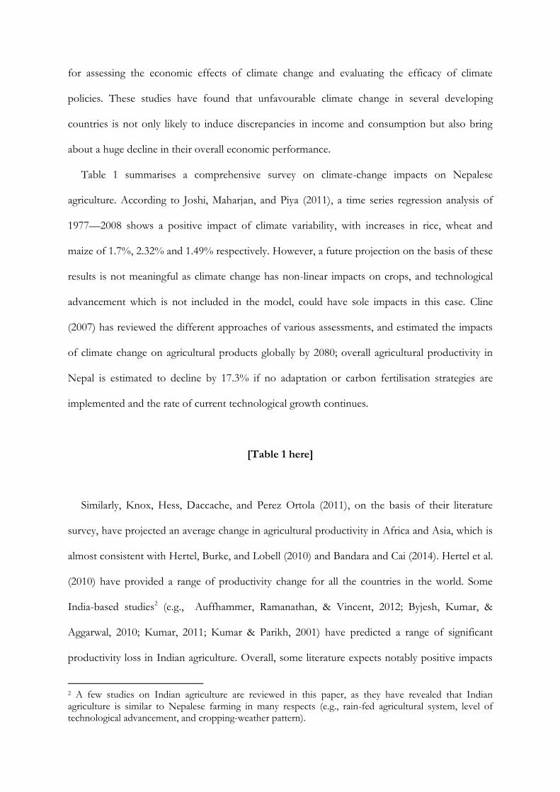
Table 1 summarises a comprehensive survey on climate-change impacts on Nepalese

agriculture. According to Joshi, Maharjan, and Piya (2011), a time series regression analysis of

1977—2008 shows a positive impact of climate variability, with increases in rice, wheat and

maize of 1.7%, 2.32% and 1.49% respectively. However, a future projection on the basis of these

results is not meaningful as climate change has non-linear impacts on crops, and technological

advancement which is not included in the model, could have sole impacts in this case. Cline

(2007) has reviewed the different approaches of various assessments, and estimated the impacts

of climate change on agricultural products globally by 2080; overall agricultural productivity in

Nepal is estimated to decline by 17.3% if no adaptation or carbon fertilisation strategies are

implemented and the rate of current technological growth continues.

[Table 1 here]

Similarly, Knox, Hess, Daccache, and Perez Ortola (2011), on the basis of their literature

survey, have projected an average change in agricultural productivity in Africa and Asia, which is

almost consistent with Hertel, Burke, and Lobell (2010) and Bandara and Cai (2014). Hertel et al.

(2010) have provided a range of productivity change for all the countries in the world. Some

India-based studies2 (e.g., Auffhammer, Ramanathan, & Vincent, 2012; Byjesh, Kumar, &

Aggarwal, 2010; Kumar, 2011; Kumar & Parikh, 2001) have predicted a range of significant

productivity loss in Indian agriculture. Overall, some literature expects notably positive impacts

2 A few studies on Indian agriculture are reviewed in this paper, as they have revealed that Indian agriculture is similar to Nepalese farming in many respects (e.g., rain-fed agricultural system, level of technological advancement, and cropping-weather pattern).

of climate change in certain crops. For example, rice yields are expected to increase till 2030, and

some assessments (e.g., Iglesias & Rosensweig, 2010; Thapa & Joshi, 2011) have projected a

positive impact of climate change on rice and wheat until 2080. Despite the variations in

estimates of productivity losses due to climate change in Nepalese agriculture, a range of these

estimations can be used as inputs for our simulation experiment.

In contrast to the existing comparative-static CGE assessments of climate-change impacts on

agriculture production (e.g., Arndt, Strzepeck, et al., 2011; Bosello & Zhang, 2005; Hertel, Rose,

Tol, Taylor, & Francis, 2009), the approach presented here is able to capture the possible land re-

allocation for several crops.

Although recent studies (e.g., Fujimori, Hasegawa, Masui, & Takahashi, 2014; Hertel et al.,

2010; Li, Taheripour, Preckel, & Tyner, 2012; Palatnik et al., 2011) have used CET in land

substitution systems, the results have some serious limitations. First, the results are limited to a

few agricultural sectors where, we argue, there is an extreme chance of an individual sector

controlling the overall model results. Second, these studies have not tested the possibility of crop

switching with a range of CET values. As CET parameters are not econometrically estimated a

sensitivity analysis of CET parameter values would give more robust results. These limitations

have created a serious gap in the evidence based policy recommendations, in which the

implication of such beneficial land re-allocation to local farmers is missing.

In this study we develop a multi-houshold CGE model for Nepal to analyse the impact of

climate change on the agriculture sector and also to examine the economic impact of land re-

allocation as an adaptation straergy to minimise the cost of climate change, and to reduce

poverty. A recent study on climate change adaptation (Chalise & Naranpanawa, 2016) has used a

framework of land-use change to see the benefits in Nepalese agricultural system, however, the

study has not analysed the changes in poverty level due to climate change impacts and

adpatation. To the best of our knowledge this is the first attempt in Nepal to analyse the

relationship of climate change impacts as well as an adaptation startegy with poverty, using the

general equilibrium framework. In this model we attempt to model the land supply using a

nested Constant Elasticity of Transformation (CET) functional form.

Therefore, the main objective of this paper is to modify the widely used assumption of “fixed

land supply for a given industry” in CGE models, by allowing farmers to supply land to crops

that are less affected by climate change, subject to any agronomic constraints; and to examine the

economy-wide impacts, industry impacts and household level impacts including household

poverty of climate change-induced agricultural loss both “with” and “without” land re-allocation

in Nepal.

The rest of the paper is organised as follows: next section illustrates the model, including the

modifications to land re-allocation function. Section 3 depicts the simulation results; and Section

4 presents some conclusions.

2. The Model

When quantifying climate-change impacts and possible adaptation strategies in agriculture, it

is difficult to assess the effects of all the factors that are being driven by climate change. The

CGE models have frequently been used to model the economy-wide impacts of different shocks

acting individually or collectively on a single country or multiple countries. Hence, a CGE model

makes an ideal analytical framework to model the climate change impacts and adaptation

strategies simultaneously on a single country. However, the recent studies which used global

CGE models (e.g., Hertel et al., 2010; Müller & Robertson, 2014; Nelson & Shively, 2014) and

South Asian CGE models (e.g., Ahmed & Suphachalasai, 2014; Bandara & Cai, 2014) to evaluate

climate-change impacts on agriculture have created a substantial research gap by ignoring the

potential impact of climate change adaptations by farmers. Thus, a single-country, multi-

household CGE model with the appropriate inclusion of potential adaptations in agriculture can

capture the discrepancies in income and consumption as well as changes in household-level

poverty due to climate-change-induced impacts in agriculture.

This paper uses a comparative-static CGE model, based on the ORANI-G model, following

the tradition of the applied general equilibrium approach pioneered by Dixon, Parmenter,

Sutton, and Vincent (1982). This Nepal CGE model (hereafter GEMNEP) modifies the South

African CGE model developed by Horridge et al. (1995), and closely follows the Nepalese CGE

model developed by Chalise and Naranpanawa (2016). As in any generic CGE model, producers

are assumed to maximise profits subject to resource constraints and consumers are assumed to

maximise utility subject to budget constraints. Moreover, this model also follows other

assumptions: export demand is negatively related to export prices; government expenditure is

exogenously determined; consumers, producers and other agents are assumed to be price takers,

not price makers; and the entire product and factor markets follow the market-clearing

assumption of demand equals supply.

This model consists of 57 industries, 57 commodities, 3 factors, 7 household groups and 10

skill/occupation types (see Appendix C and D). Household incomes are determined by their

possession of 3 production factors (land, labour and capital) and the market returns to these

factors. The model comprises a set of nested Constant Elasticity of Substitution (CES) functions

for specifying production technologies and consumer demands for final goods and services.

Households, government and the rest of the world are the major agents that demand the final

goods for their consumption. In the same way, we specify a CES function for an intermediate

mix. Production of final goods and services is the combination of intermediate inputs and

primary factors. The primary factors (land, labour and capital) are aggregated through a CES

function with a sub-set of CES functions for different types of occupations and a CET function

for land supply (see the CET specification in the next part of this section).

In order to incorporate the key characteristics of household types, occupational skills and

their linkages to the rest of the economy, we extend the basic CGE model in two dimensions.

First, given that a comparative analysis of climate-change impacts is important for identifying

winners and losers, we follow Horridge et al. (1995) and Chalise and Naranpanawa (2016) and

introduce seven types of households on the basis of their characteristics, such as hectares of

agricultural land that they hold and household head’s level of education (see Appendix C). The

purpose of defining household groups in this way is to introduce heterogeneity with respect to

urban/rural livelihood, mountain/hill/lowland topography, and high/low education. In doing

so, we use the Nepalese National Living Standard Survey database (CBS, 2011b) to disaggregate

households’ final consumption and returns from primary factors. Second, to allow for

differential effects in the employment of skill categories, we introduce 10 occupation types and

explicitly model the heterogeneity of levels of income.

[Diagram 1 here]

In this model, “Rest of the world” is an agent that links the exports and imports of goods and

services with the national economy. In this case, a CES function is also specified to represent

consumers’ choices/decisions between domestic and imported goods, aggregating the final

demand composite. The relative prices of goods and services are determined on the basis of real

exchange rate as a numeraire such that income in household level is influenced by relative prices

rather than absolute ones. To represent that saving equal investment, savings-driven income flow

is assumed analogous to investments that are used only for final commodities. Capital and labour

are perfectly mobile within the industry sectors. As there is a scientific consensus that the

impacts of climate change can be realised distinctly within a 30—40 year period, a long-run

closure (see Diagram 1) is set for our model simulation to avoid the uncertainty of transitional

projection. At the macro-level, GDP, household consumption, investment, public spending, real

wages and capital stock are treated as endogenous. Total employment, technical changes, capital

rate of return and terms of trade are treated as exogenous.

CET function of land re-allocation

The proposed model adds an important land supply equation to the original ORANI-G

model, including linearisation of profit maximisation subject to the cost of inputs. As land rentals

across different land usage suggest that land does not move freely between alternatives, the only

way to model land supply is to use a CET function. In doing so, we assume that producers seek

to maximise returns from land producing given levels of output by supplying extra land to

industries that experience significantly fewer impacts of climate change. Thus, the maximisation

of return can be presented as a constrained optimisation problem, where producers choose land,

Xi (i = 1… k……..n), to maximise the total returns from the inputs of producing a given output,

Y, subject to the CET production function:

𝑌 = [∑ 𝛿𝑖𝑛𝑖=1 𝑋𝑖

𝜌]

1/𝜌 (1)

and objective function: 𝑀𝑎𝑥 𝑇𝑅 = ∑ 𝑃𝑖𝑋𝑖𝑛𝑖=1

Where, 𝛿 is share of land, and 𝛿0. and 𝜌 are parameters, and 𝜌 1. 𝑋𝑖 is a plot of land

allocated, for i is equal to 1 to ‘n’ crops. Pi is profit of an effective land unit. 𝛿𝑖 and 𝜌 are

behavioural parameters and TR is the total revenue generated from the land. To solve the model

in the level forms, the values of 𝛿𝑖 are normally determined in a base-year calibration procedure.

The land area balance is therefore maintained in the base year. However, area balance is not

guaranteed if either the relationship among the nested land shares or the relative prices are

changed from the values used in the calibration. To fix the Xi, it is natural to allocate arbitrary

values to Pk, say 1. This simply sets appropriate units for the Xi (in base-period-dollars).

The Lagrangian equation for the above problem can be written as follows:

𝐿 = ∑ 𝑃𝑖𝑋𝑖𝑛𝑖=1 + 𝛬 [𝑌 − (∑ 𝛿𝑖

𝑛𝑖=1 𝑋𝑖

𝜌)

1

𝜌] (2)

From which (see Equation E3 to Equation E13 in Appendix D for the complete derivation),

we have, for a particular industry, k:

𝑋𝑘 = 𝑌 {∑ 𝛿𝑖 (𝑃𝑖𝛿𝑘

𝑃𝑘𝛿𝑖)

𝜌

(𝜌−1)𝑛𝑖=1 }

−1

𝜌

(3)

Equation (4) can be transformed into a linear percentage form as follows:

𝑥𝑘 = 𝑧 − 𝜎(𝑝𝑎𝑣𝑒 − 𝑝𝑘) (4)

Where, z is the total agricultural land, 𝑥𝑘 is the land allocated for a particular industry, k, and

maximising the return from a unit plot of land is the principal objective of the producers. This is

determined by farmers’ decisions with respect to the degree of impact of climate change to that

particular crop. 𝜎 is the CET parameter that is externally supplied in the model on the basis of

agronomic feasibility. Mathematically, 𝜎 = 1(𝜌 − 1)⁄ . Similarly, 𝑝𝑘 is the profitability per unit

of effective land and 𝑝𝑎𝑣𝑒 is the average profitability per unit of effective land. Mathematically,

𝑝𝑎𝑣𝑒 = ∑ 𝑆𝑖𝑖 𝑝𝑖, where, Si is the share of industry, i, in total land profitability.

In the linear form (Equation 4), 𝜎 has the most important and debatable role in determining

how each plot of land is allocated to particular crop. This is highly important because a small

change in 𝜎 significantly changes the amount of land allocated. It is debatable because its value is

supplied from outside. Unlike the CES function, the higher the value of 𝜎, the greater the chance

of allocating land to that particular crop. However, another factor determining the land

allocation to a particular crop is profitability (𝑝𝑘). Suppose that there is a hypothetical land plot

and its use is to be decided according to the profitability from the crop planted. In this case, a

detailed study on the agronomic feasibility of crop switching is required. It is irrelevant to use

historical crop yielding to determine the land’s profitability, as future impacts of climate change

can substantially change its status. Therefore, this paper has linked climate change—induced

productivity change with the profitability of crops in Nepal.

A problem with the CET function is that it implies that the elasticity of transformation is

identical for all pairs of crops (Powell & Gruen, 1968). It is almost impossible to use Equation 4

to address the heterogeneity of several agricultural sectors. The only way to deal with this

problem is by arranging the CET function in a nest. In doing so, the arguments of the function

are split into pairs. Again, a major problem in nested CET functions is how to choose the pairs

in a nest: this depends on agronomic characteristics and constraints. Because of these

constraints, a set of pairs may include different crops in different agro-ecological zones. To

address this issue, our model has used a set of CET parameters to test a range of climate change

impacts on the overall economy.

As the main objective of this paper is to develop and test a general framework of land re-

allocation, we develop a simple nest of CET functions with two levels. Out of 14 agricultural

sectors, a nest of the paddy sector and other agricultural sectors is developed. A set of CET

values is used to model the transferring the paddy land into the other 13 agricultural lands and

vice versa. Similarly, a set of CET values is used to model transferring land between other pairs

of crops within the 13 agricultural sectors. Although previous studies (e.g., Keeney & Hertel,

2009; Palatnik et al., 2011) have attempted to develop a nested set of agricultural sectors, their

results are seriously limited by not testing a range of CET values for a single pair. It is difficult to

recommend a land re-allocation framework without testing a set of feasibility parameters.

Therefore, we develop a wide range of CET values, from highly inelastic to elastic to highly

elastic, to test their feasibility and to recommend a framework to the local farmers of Nepal.

[Diagram 2 here]

In order to address the link between climate change—induced impacts in agricultural

productivity and other parameters in the overall economy, we focus on the 14 agricultural

industries3 (out of the 57 sectors in the GTAP database— see Appendix D) in Nepal. From the

impact assessment—related literature, a range of productivity shocks of rice, wheat, maize and

other agricultural products are employed in the CGE model developed for this study (see Table

3 Rice, wheat, cereal grains, vegetables fruits and nuts, oil seeds, sugar cane sugar beet, plant based fibers, other crops, bovine cattle sheep goats horses, animal products, raw milk, wool silk worms, forestry and fishing

2). The reasons for taking a range of impacts are, firstly, to address the irregular trend of

assessment developed in previous literature. Secondly, the previous assessments have a different

time frame of impact assessment, with the risk of extremely low or high estimations. Three

scenarios (highest, medium and lowest) are developed for the simulations in this paper. Each

scenario comprises three simulations. Diagram 2 presents the conceptual framework. Simulations

H1, M1 and L1 assume that normal land allocation prevails and there is no change in land supply

with respect to impacts of climate change. Each scenario has two other simulations, assuming

that the land is mobile among industries. The first simulations (H2, M2 and L2) assume that the

CET of paddy (CET1) is less than the CET of other agricultural sectors (CET2); and the second

that CET1 is greater than CET2. The results are compared and analysed on the basis of changes

in key macro-variables such as real GDP, real wages, household consumption and industry

output.

[Table 2 here]

To analyse the discrepancies in household poverty level, this study attempts to measure

income poverty within the seven household groups, namely, rural land-less households, rural

land-small households, rural land-medium households, rural land-large households, urban low-

education households, urban medium-education households and urban high-education

households. A reason of classifying the household groups in this way is that income in rural areas

of Nepal primarily depends on agricultural land owned by the households whereas urban

household-incomes depend on level of education hold by household head (see detail household

categories in Appendix C). In order to compare the pre- and post-simulation absolute poverty,

the most popular money metric poverty indices of Foster, Greer and Thorbecke (FGT) (Foster,

Greer, & Thorbecke, 1984) is considered. Changes in income due to climate-change impacts and

land re-allocation in different seven household groups are adjusted to compare the poverty level.

Poverty line also changes with changes in price level (Naranpanawa, Bandara, & Selvanathan,

2011). To address this issue of price change, changes in consumer price index (CPI) are used to

determine the poverty line for each household in each simulation.

The overall base year poverty line is obtained by aggregating the food and the non-food

poverty lines. The poverty line for Nepal, in average 2010–11 prices, has been estimated at Rs.

19,261; the food poverty line is Rs. 11,929 and the non-food poverty line is Rs. 7,332. The

aggregated poverty line is used for this study. However, a set of poverty lines is used for seven

different household groups for this study (see Table 3).

[Table 3 here]

3. Simulation Results

The results obtained from the simulations of the impacts of climate change and land re-

allocation on Nepalese agriculture are analysed in three different stages: (1) changes in the overall

macro-variables; (2) impacts at the industry level; and (3) impacts at the household level. As

mentioned in the model section, every result is compared to the baseline status and reported as a

percentage change. Deviation of the variables from the base year (a year without climate change

and land re-allocation; our model uses 2011 as the base year) to a future year (which is

determined with distinct climate-change impacts and land re-allocation; our model uses 2080) is

evaluated. As demonstrated in Diagram 2, three distinct climate change scenarios (highest,

medium and lowest) are simulated. In each climate change scenario, there are three simulations.

In simulation 1 of each climate change impact scenario, the effects of climate change on poverty

are analysed assuming that normal land allocation prevails and that the effects of land re-

allocation among agricultural sectors can be ignored. In simulation 2 and 3 of respective climate

change impact scenarios, crop switching by farmers to increase the availability of land to crops

less impacted by climate change is represented by changes in the amount of farmland under less-

impacted crops. As discussed in the previous section, simulation 2 and 3 are analysed with two

different experiments on the basis of CET ratio: simulation 2 has CET1 < CET2 and simulation

3 has CET1 > CET2 (CET values range from 0.05 to 20).

Impacts in macro-variables

The percentage change results of important macro-economic variables over the base year

values for above simulation experiments are summarised in Table 4.

[Table 4 here]

Real GDP is an important tool for evaluating a change in the overall economy due to the

impacts of climate change and land re-allocation on agriculture. Moreover, the use of real GDP

in terms of estimating changes in the Nepalese economy is important, as agriculture represents

around 36% of the national GDP. Table 4 shows that, without land re-allocation, the projected

impact of climate change on agricultural productivity affects real GDP negatively. In simulation

1, the real GDP is expected to decrease by 10.92% by 2080 in the highest impact scenario if

smallholders do not adopt the land re-allocation strategy. Similarly, land transformation from

paddy to other agricultural sectors may lead to a decrease in real GDP by 11.76%, which is again

a worse situation than before. However, a correct way of land transformation (for example,

simulations H3, M3 and L3) can lead to a better real GDP, such as a loss of only 9.66% in H3

simulation. In between simulation H2 and H3, the change in real GDP depends on the CET

ratio. The higher the CET ratio, the less are the impacts of climate change on real GDP. A

higher CET ratio means farmers are expected to re-allocate more land to less climate change

impacted crops, such as paddy, from high climate change impacted crops such as maize. A

similar trend of change in real GDP can be expected in the other two (medium and lowest)

scenarios (see Table 4). A major factor of such a significant fall in GDP is the substantial fall in

output of many agricultural products and other industrial outputs related to agriculture.

Regarding simulations 2 and 3, the change in real GDP depends on the CET ratio. The higher

the CET ratio, the less the impacts of climate change on real GDP.

In the long-run simulations, it is assumed that the aggregate employment is fixed and thus the

economy is in full employment. However, labour is allowed to be mobile between industries as

well as between different labour categories. Implications of the above simulations on these

labour movements are presented in terms of real wage (see Table 4). In the long-run closure, it is

assumed that real wages are determined endogenously. Table 4 demonstrates the improvement in

the real wages after simulation with land re-allocation strategy. The increase in real wages is due

to the increase in the derived demand for labour, as a result of considerable expansion in

activities of agricultural industries. Real GDP from the supply side is mainly determined by real

wages.

Land re-allocation as climate-change adaptation in the long run improves real GDP. To

understand the factors contributing to this change, the changes in each aggregate making up

GDP from expenditure side should be decomposed. On the expenditure side, growth is mainly

due to contributions from real household consumption (from -9.88% to -10.11% to -8.44% in

the highest impact scenario, from -7.61% to -8.27% to -6.98% in the medium impact scenario,

and from -2.36% to -3.18 to -1.97% in the lowest impact scenario). Consumer price index is also

improved while comparing without and with land re-allocation as climate change adaptation

strategy.

Impacts at industry level

Overall sectoral outputs are likely to be affected according to climate change—induced

productivity loss in Nepalese agriculture. Table 5 shows the decrease in sectoral output and the

improvement that can be achieved with land re-allocation. The climate-change impacts without

any adaptation strategy lead to an increase in the cost of production as domestic and imported

inputs become expensive. The implementation of land re-allocation as an adaptation strategy

against climate change reduces the cost of production, as inputs become less expensive than

without any sort of adaptation. As the consumer price index (CPI) goes high in the climate

change scenarios without land re-allocation, the nominal wage rate goes high. However, land re-

allocation helps to reduce CPI, resulting in a reduction in the nominal wage rate.

[Table 5 here]

As noted in Table 5, the manufacturing industries, along with the expansion of the

agricultural industries, are also expected to expand significantly when farmers allocate more land

to crops less impacted by climate change. In particular, industries such as dairy products, food

products and processed rice have shown a marked increase in output while increasing the CET

ratio, reflecting more land transformation possibilities. For example, the food production

industry has shown a significant increase in output, from -14.79% to -6.32% in the highest

impact scenario; from -11.47% to around -3% in the medium impact scenario; and from -2.42%

to 5.41% in the lowest impact scenario. These improvements are responsible for the overall

improvement in the manufacturing sector. Similarly, other industries such as dairy products and

vegetable oils and fats have made a slight improvement in the output while increasing the CET

ratio.

Impacts at household level

A substantial decrease in sectoral outputs, primarily in agricultural products, influences

household income and consumption. To understand the considerable loss in GDP requires an

estimation of the change in the individual parameters that determine the real GDP from the

income side: land rents, labour wages, capital interests, profits and taxes. The major components

of household income are rental income, wages and interest. We have to investigate the income of

rural and urban households separately. As total employment is constant in the long run closure

of the model, labour from other sectors moves to agriculture-based industries. As the cost of

living goes up due to extreme inflationary prices, overall real wages decrease significantly.

However, land re-allocation to climate-smart crops such as paddy can improve the loss in

sectoral outputs and recover some of the household income and expenditure (see Table 6 and 7).

[Table 6 here]

As real GDP (from the expenditure side—see the last row of Diagram 1) is determined by the

sum of household consumption, investment, government expenditure and net exports, the

significant decrease in household consumption results in a huge decline in real GDP. Overall

household consumption, which is shown in Table 4, clearly illustrates the important role of

household expenditure in maintaining a progressive GDP. To understand the full effects of

climate change—induced productivity loss, it is important to see the differences in impacts

between various households. Table 7 shows the changes in consumption for different household

groups. The table clearly differentiates the spread of impacts, as urban households are expected

to experience a significantly greater decrease in consumption than rural ones. This is because

urban households do not produce agricultural commodities and depend on highly priced

products from the producers, who primarily belong to rural households. However, the patterns

of consumptions are projected to improve if farmers allocate land to paddy as expected.

[Table 7 here]

[Table 8 here]

The FGT indicators are estimated and compared with the base case and their percentage

changes from the base case are reported in Table 8. Positive change of FGT index denotes an

increment in absolute poverty. As can be seen from this table under the base year simulation and

simulation without adaptation, the poverty headcount ratios have increased significantly among

all household groups. Simulation 3 of each climate change impact scenario shows how land re-

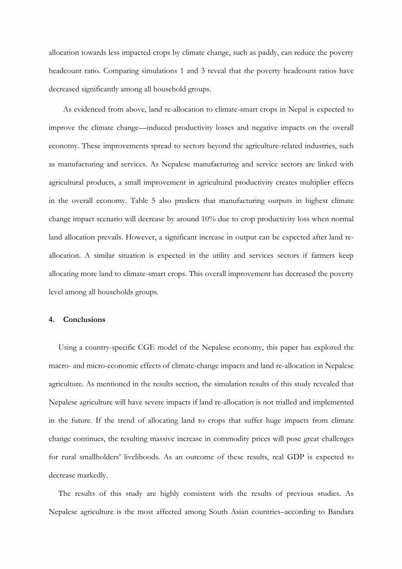
allocation towards less impacted crops by climate change, such as paddy, can reduce the poverty

headcount ratio. Comparing simulations 1 and 3 reveal that the poverty headcount ratios have

decreased significantly among all household groups.

As evidenced from above, land re-allocation to climate-smart crops in Nepal is expected to

improve the climate change—induced productivity losses and negative impacts on the overall

economy. These improvements spread to sectors beyond the agriculture-related industries, such

as manufacturing and services. As Nepalese manufacturing and service sectors are linked with

agricultural products, a small improvement in agricultural productivity creates multiplier effects

in the overall economy. Table 5 also predicts that manufacturing outputs in highest climate

change impact scenario will decrease by around 10% due to crop productivity loss when normal

land allocation prevails. However, a significant increase in output can be expected after land re-

allocation. A similar situation is expected in the utility and services sectors if farmers keep

allocating more land to climate-smart crops. This overall improvement has decreased the poverty

level among all households groups.

4. Conclusions

Using a country-specific CGE model of the Nepalese economy, this paper has explored the

macro- and micro-economic effects of climate-change impacts and land re-allocation in Nepalese

agriculture. As mentioned in the results section, the simulation results of this study revealed that

Nepalese agriculture will have severe impacts if land re-allocation is not trialled and implemented

in the future. If the trend of allocating land to crops that suffer huge impacts from climate

change continues, the resulting massive increase in commodity prices will pose great challenges

for rural smallholders’ livelihoods. As an outcome of these results, real GDP is expected to

decrease markedly.

The results of this study are highly consistent with the results of previous studies. As

Nepalese agriculture is the most affected among South Asian countries–according to Bandara

and Cai (2014) and Chalise et al. (2017), among others–the results of the simulation described

above show that climate-induced reduction in food production is projected to put an upward

pressure on food prices, resulting in a food security problem in Nepal. The prices of rice, wheat

and cereal grains—three major staple foods in Nepal—are expected to rise significantly at the

rate of around 26%, 36% and 44% per annum respectively. As Nepal imports most of its staples

foods from South Asian countries, the situation will become challenging as global food prices are

expected to increase significantly in the future (FAO, 2015; Hertel et al., 2010).

Some key policy implications related to climate change, particularly from a larger perspective,

can be drawn from this study. Nepal, as a member of the least-developed countries, can expect

the impacts of climate change to be severe. Mainly because of its static adaptation capacity,4 the

vulnerability projection according to the A2 emission scenario in 2050 (IPCC, 2000) places

Nepal in the significantly vulnerable category. Although farmers have already initiated some

useful adaptation practices on their own, without any support from government or any other

organisations, it is urgent to initiate large-scale planned strategies to support them. Based on the

results of this study, as well as the likelihood of more frequent flash floods in low-land paddy

farms and serious landslides in hilly maize farms in Nepal, it seems wise to invest more in

controlling excess water flows and on forest management technology. In addition, serious

consideration should be given to measures designed to prevent, mitigate and adapt to water

deficiency in Nepalese cropping agriculture. As Salami, Shahnooshi, and Thomson (2009)

suggest, cropping rotation and changes in the cropping-calendar, such as fairly simple

modifications in vegetable growing (changed planting dates, and different maturity-date

cultivars), can reduce likely climate change—induced losses in future decades.

To conclude, future research is recommended to address the limitations of this study. Our

study has not explored the bio-physical aspects of climate-change impacts in detail, including

4 According to the vulnerability projection report, vulnerability is a function of exposure, sensitivity and adaptive capacity.

those determining the actual cost of damage to crops and human capital, such as impacts in bio-

physical requirements due directly or indirectly to imbalances in water, or to labour productivity,

etc. Therefore, a study to evaluate all the factors responsible for productivity loss due to climate

change, and the adaptation practices that have been started in Nepal, is required. A numerical

assessment of the impacts and possible adaptation to climate change would require a much

expanded modelling framework, and/or considered assumptions of the extent and distribution

of such problems. Despite this study’s limitations, its results have evidenced that serious policy

planning and implementation of adaptation strategies in the near future is required to help

reduce the negative impact of climate change on agriculture and to reduce the level of poverty

among all household groups.

Appendix A

Table 1 Comprehensive literature survey on climate-change impacts in Nepalese agriculture

Source Methodology Crop Productivity change (%)

Kumar and Parikh (2001) Regression on net farm revenue All -8.4 (Projection in Indian crops- as of +2oC)

Cline (2007) Integrating all models

All Without carbon fertilisation = -17.3 With carbon fertilisation and adaptation = -4.8

Iglesias and Rosensweig (2010)

Crop simulations on the basis of carbon dioxide emission scenarios5

Rice Wheat Maize

2020 2050 2080 -2.23 +2.70 +6.67 -7.55 +9.58 +9.37 -7.75 -10.91 -4.98

Hertel et al. (2010) General equilibrium analysis based on GTAP

Rice Wheat Maize

Low Medium High -15 -5 +4 -10 -3 +4 -17 -10 -3

Joshi et al. (2011) Time Series Regression (1977-2008 as of +20C)

Rice Wheat Maize

+1.7 +2.32 +1.49

Knox et al. (2011) Crop models Rice Wheat Maize

2020 2050 2080 -2 -32 -60 (Indian crops) +10 (other SA countries)

Bandara and Cai (2014) Systematic literature review on all models

Rice Wheat Maize

-2 -13.7 -17 (2030 projection)

Note: This table is mainly based on a systematic literature survey and is adapted from Chalise et al. (2017)

5 The data are available for different CO2 emission scenarios of SRES (IPCC, 2000). The A2 scenario is employed for this study.

Diagram 1. Long-run closure used in the model. Note: The exogenous and endogenous variables used in this model closure are based on recent ORANI-G version. Source: Chalise et al. (2017)

Employment Technical Change Land

Tax rates Return to capital

Taxes

GDP

Consumption Government Investments

Capital

stocks

Return to

land Real wage

+

+ + + +

+ + +

Residual: Move together to satisfy

trade balance constraint

Follow sales Follow capital

stocks

Fixed share of

GDP

Key

Endogenous Exogenous

X - M Inventories

Diagram 2. Conceptual framework of the experiment Note: H1, H2, H3, M1, M2, M3, L1, L2 and L3 are simulations.

Table 2 Climate change induced productivity shocks used in the model (%)

Sector Highest climate change impact scenario (H)

Medium climate change impact scenario (M)

Lowest climate change impact scenario (L)

Paddy Rice -14.10% -10.81% -1.20%

Wheat -18.90% -14.16% -2.30%

Maize -24.70% -19.08% -6.90%

Other agricultural sectors -19.30% -14.67% -4.80%

Note: This table is mainly based on a systematic literature survey and is based on Table 1.

Database for year 2011 – without climate change

impacts and land re-allocation

BASELINE

RESULTS

GDP

Real wages

Households Consumption

Sectoral output

Total output

Poverty Level

Highest climate change impact scenario (H)

H1: NO ADAPTATION

Medium climate change impact scenario (M)

Lowest climate change

impact scenario (L)

H2: CET1<CET2

H3: CET1>CET2

M1: NO ADAPTATION

M2: CET1<CET2

M3: CET1>CET2

L1: NO ADAPTATION

L2: CET1<CET2

L3: CET1>CET2

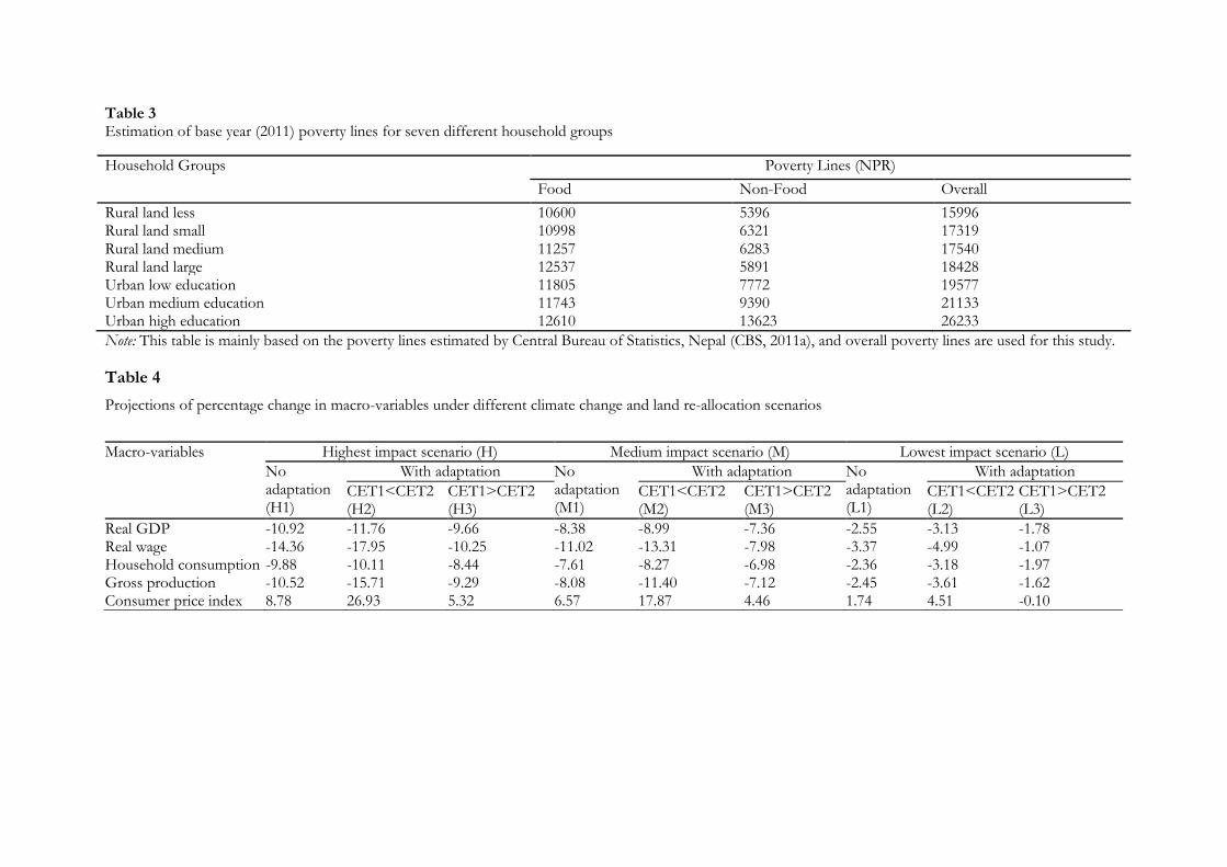
Table 3 Estimation of base year (2011) poverty lines for seven different household groups

Household Groups Poverty Lines (NPR)

Food Non-Food Overall

Rural land less 10600 5396 15996 Rural land small 10998 6321 17319 Rural land medium 11257 6283 17540 Rural land large 12537 5891 18428 Urban low education 11805 7772 19577 Urban medium education 11743 9390 21133 Urban high education 12610 13623 26233

Note: This table is mainly based on the poverty lines estimated by Central Bureau of Statistics, Nepal (CBS, 2011a), and overall poverty lines are used for this study.

Table 4

Projections of percentage change in macro-variables under different climate change and land re-allocation scenarios

Macro-variables Highest impact scenario (H) Medium impact scenario (M) Lowest impact scenario (L)

No adaptation (H1)

With adaptation No adaptation (M1)

With adaptation No adaptation (L1)

With adaptation

CET1<CET2 (H2)

CET1>CET2 (H3)

CET1<CET2 (M2)

CET1>CET2 (M3)

CET1<CET2 (L2)

CET1>CET2 (L3)

Real GDP -10.92 -11.76 -9.66 -8.38 -8.99 -7.36 -2.55 -3.13 -1.78 Real wage -14.36 -17.95 -10.25 -11.02 -13.31 -7.98 -3.37 -4.99 -1.07 Household consumption -9.88 -10.11 -8.44 -7.61 -8.27 -6.98 -2.36 -3.18 -1.97 Gross production -10.52 -15.71 -9.29 -8.08 -11.40 -7.12 -2.45 -3.61 -1.62 Consumer price index 8.78 26.93 5.32 6.57 17.87 4.46 1.74 4.51 -0.10

Table 5

Projections of percentage change in industry output of commodities under different climate change and land re-allocation scenarios

Sectors Highest impact scenario (H) Medium impact scenario (M) Lowest impact scenario (L)

No adaptation (H1)

With adaptation No adaptation (M1)

With adaptation No adaptation (L1)

With adaptation

CET1<CET2 (H2)

CET1>CET2 (H3)

CET1<CET2 (M2)

CET1>CET2 (M3)

CET1<CET2 (L2)

CET1>CET2 (L3)

Agriculture -12.99 -14.30 -11.35 -10.08 -10.95 -9.00 -3.24 -4.04 -2.36 Mining -13.96 -36.08 -12.08 -10.55 -24.52 -9.10 -2.95 -6.49 -1.48 Manufacture -10.07 -16.89 -8.77 -7.72 -12.07 -6.67 -2.30 -3.64 -1.32 Utilities -7.55 -7.84 -6.74 -5.76 -6.01 -5.22 -1.73 -2.12 -1.38 Services -8.13 -10.17 --7.11 -6.19 -7.53 -5.62 -1.84 -2.46 -1.42

Table 6

Projections of percentage change in total household income under different climate change and land re-allocation scenarios

Sectors Highest impact scenario (H) Medium impact scenario (M) Lowest impact scenario (L)

No adaptation (H1)

With adaptation No adaptation (M1)

With adaptation No adaptation (L1)

With adaptation

CET1<CET2 (H2)

CET1>CET2 (H3)

CET1<CET2 (M2)

CET1>CET2 (M3)

CET1<CET2 (L2)

CET1>CET2 (L3)

Rural land less -13.25 -13.53 -10.94 -10.20 -10.80 -8.69 -3.14 -3.71 -2.03 Rural land small -11.64 -12.42 -8.21 -8.94 -9.45 -6.70 -2.77 -3.76 -1.12 Rural land medium -11.02 -11.18 -8.84 -8.49 -8.74 -7.38 -2.65 -2.83 -1.90 Rural land large -11.04 -11.94 -9.76 -8.53 -8.87 -8.17 -2.67 -2.82 -2.51 Urban low education -15.17 -18.18 -11.74 -11.66 -13.60 -9.03 -3.56 -4.97 -1.56 Urban medium education -15.25 -15.40 -12.65 -11.74 -11.89 -9.89 -3.61 -4.39 -2.22 Urban high education -14.55 -14.67 -12.45 -11.22 -11.41 -9.89 -3.46 -3.82 -2.50

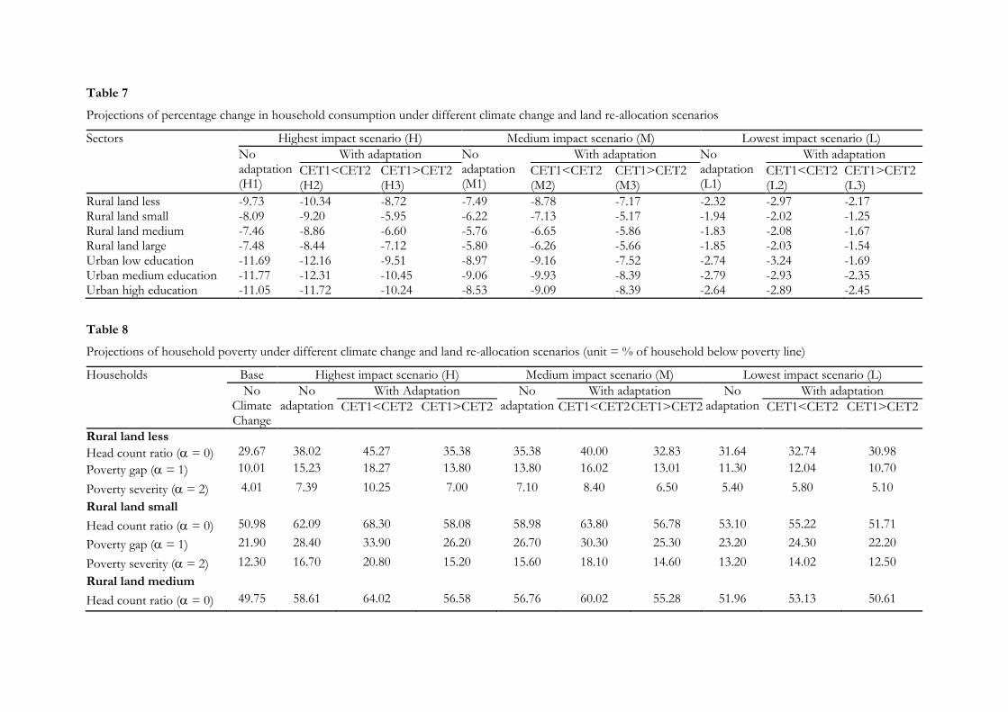
Table 7

Projections of percentage change in household consumption under different climate change and land re-allocation scenarios

Sectors Highest impact scenario (H) Medium impact scenario (M) Lowest impact scenario (L)

No adaptation (H1)

With adaptation No adaptation (M1)

With adaptation No adaptation (L1)

With adaptation

CET1<CET2 (H2)

CET1>CET2 (H3)

CET1<CET2 (M2)

CET1>CET2 (M3)

CET1<CET2 (L2)

CET1>CET2 (L3)

Rural land less -9.73 -10.34 -8.72 -7.49 -8.78 -7.17 -2.32 -2.97 -2.17 Rural land small -8.09 -9.20 -5.95 -6.22 -7.13 -5.17 -1.94 -2.02 -1.25 Rural land medium -7.46 -8.86 -6.60 -5.76 -6.65 -5.86 -1.83 -2.08 -1.67 Rural land large -7.48 -8.44 -7.12 -5.80 -6.26 -5.66 -1.85 -2.03 -1.54 Urban low education -11.69 -12.16 -9.51 -8.97 -9.16 -7.52 -2.74 -3.24 -1.69 Urban medium education -11.77 -12.31 -10.45 -9.06 -9.93 -8.39 -2.79 -2.93 -2.35 Urban high education -11.05 -11.72 -10.24 -8.53 -9.09 -8.39 -2.64 -2.89 -2.45

Table 8

Projections of household poverty under different climate change and land re-allocation scenarios (unit = % of household below poverty line)

Households Base Highest impact scenario (H) Medium impact scenario (M) Lowest impact scenario (L)

No Climate Change

No adaptation

With Adaptation No adaptation

With adaptation No adaptation

With adaptation

CET1<CET2 CET1>CET2 CET1<CET2 CET1>CET2 CET1<CET2 CET1>CET2

Rural land less

Head count ratio ( = 0) 29.67 38.02 45.27 35.38 35.38 40.00 32.83 31.64 32.74 30.98

Poverty gap ( = 1) 10.01 15.23 18.27 13.80 13.80 16.02 13.01 11.30 12.04 10.70

Poverty severity ( = 2) 4.01 7.39 10.25 7.00 7.10 8.40 6.50 5.40 5.80 5.10

Rural land small

Head count ratio ( = 0) 50.98 62.09 68.30 58.08 58.98 63.80 56.78 53.10 55.22 51.71

Poverty gap ( = 1) 21.90 28.40 33.90 26.20 26.70 30.30 25.30 23.20 24.30 22.20

Poverty severity ( = 2) 12.30 16.70 20.80 15.20 15.60 18.10 14.60 13.20 14.02 12.50

Rural land medium

Head count ratio ( = 0) 49.75 58.61 64.02 56.58 56.76 60.02 55.28 51.96 53.13 50.61

Poverty gap ( = 1) 22.30 28.20 32.07 26.66 26.76 29.24 25.81 23.61 24.43 22.88

Poverty severity ( = 2) 12.90 17.08 19.93 15.94 16.02 17.83 15.34 13.80 14.36 13.29

Rural land large

Head count ratio ( = 0) 37.79 46.41 51.67 43.06 43.06 46.88 42.58 39.23 40.19 38.75

Poverty gap ( = 1) 16.69 21.20 23.75 20.20 20.05 21.65 19.51 17.64 18.15 17.21

Poverty severity ( = 2) 9.96 12.97 14.67 12.29 12.19 13.27 11.82 10.58 10.91 10.30

Urban low education

Head count ratio ( = 0) 27.62 39.18 48.04 36.66 37.01 41.44 34.40 29.80 32.49 28.14

Poverty gap ( = 1) 11.86 16.72 21.35 15.22 15.36 18.14 14.34 12.75 13.50 12.10

Poverty severity ( = 2) 6.69 9.69 12.68 8.78 8.86 10.60 8.24 7.26 7.73 6.85

Urban med. education

Head count ratio ( = 0) 11.26 18.87 28.16 17.18 16.90 22.25 15.40 12.11 13.23 11.26

Poverty gap ( = 1) 4.49 6.77 9.25 6.10 6.07 7.31 5.65 4.86 5.12 4.63

Poverty severity ( = 2) 2.49 3.71 4.86 3.38 3.36 3.98 3.15 2.72 2.87 2.58

Urban high education

Head count ratio ( = 0) 5.43 10.04 12.97 7.11 7.11 10.46 7.11 5.85 6.27 5.43

Poverty gap ( = 1) 2.32 3.30 4.30 3.02 2.99 3.50 2.84 2.49 2.60 2.40

Poverty severity ( = 2) 1.40 1.93 2.37 1.80 1.78 2.02 1.70 1.50 1.56 1.45

Note: The poverty lines for each household and each simulation (base year poverty line for rural household = averagely NRs 92738/year and base year poverty line for urban households = averagely NRs 120995/year) are determined on the basis of the poverty report prepared by central bureau of statistics, Nepal (CBS, 2011a) and changes in consumer price index (CPI) reported in Table 4.

Appendix B

Figure B1 Projection of change in daily temperature and precipitation (1999 to 2080)

Note: The Figure is mainly based on projection by Cline (2007). P0 = daily precipitation of base year-1999, P1 = projected daily precipitation of 2080, T0 = temperature of base year-1999 and T1 = projected temperature of 2080.

Appendix C

Table C1 Household groups and occupation types

Grouping Household groups and their characteristics

Households 1. Rural landless households (no agricultural land) 2. Rural land small households (less than 0.5 Bigha*) 3. Rural land medium households (between 0.51 and 2.50 Bigha) 4. Rural land large households (more than 2.51 Bigha) 5. Urban low education (household head having less than class/grade 10 education) 6. Urban medium education (household head having both secondary school certificate and higher secondary certificate) 7. Urban high education (household head having bachelor and high degrees)

Jan Feb Mar Apr May Jun Jul Aug Sep Oct Nov Dec Avg

P0 0.67 0.93 1.13 1.64 2.89 6.55 11.18 9.37 6.6 1.94 0.33 0.48 3.64

P1 0.7 0.79 0.73 1.22 3.65 8.58 16.98 12.03 8.04 2.36 0.26 0.45 4.57

T0 4.15 5.75 10.17 14.53 17.17 19.18 19.13 18.71 17.5 13.79 9.17 5.56 12.9

T1 8.93 10.7 15.24 19.58 21.78 22.92 22.17 21.83 21.19 18.1 13.19 9.98 17.13

0

5

10

15

20

25

Dai

ly T

emp

erat

ure

(o

C)

&

pre

cip

itat

ion (

mm

)

Occupations 1. Self-employed labours 2. High skilled professionals and managers 3. Medium skilled professionals and technicians 4. Government and non-government office clerks (employees) 5. Workers (transport, mechanics and other industrial workers) 6. Artisans and handicraftsmen 7. Informal (street-vendors and non-economic services nes) 8. Agricultural owners/administrators 9. Agricultural workers 10. Agriculture subsistence farmers

Note: Bigha* is a unit of land mostly used in the rural part of Nepal. One Bigha = 0.16055846 Hectares. This table is adapted from Chalise et al. (2017)

Appendix D

Table D1 List of industries

Sectors Industries

Agriculture 1. Paddy rice 2. Wheat 3. Cereal grains nec 4. Vegetables, fruit and nuts 5. Oil seeds 6. Sugar cane, sugar beet 7. Plant-based fibers 8. Crops nec 9. Bovine cattle, sheep and goats, horses 10. Animal products nec 11. Raw milk 12. Wool, silk-worm cocoons 13. Forestry 14. Fishing

Mining 15. Coal 16. Oil 17. Gas 18. Minerals nec Manufacturing 19. Bovine cattle, sheep and goat, horse meat products 20. Meat products nec 21. Vegetable oils and fats 22. Dairy products 23.

Processed rice 24. Sugar 25. Food products nec 26. Beverages and tobacco products 27. Textiles 28 Wearing apparel 29. Leather products 30. Wood products 31. Paper products, publishing 32. Petroleum, coal products 33. Chemical, rubber, plastic products 34. Mineral products nec 35. Ferrous metals 36 Metals nec 37. Metal products 38. Motor vehicles and parts 39. Tranport equipment nec 40. Electronic equipment 41. Machinery and equipment nec 42. Manufacturers nec

Utilities 43. Electricity 44. Gas manufacture, distribution 45. Water Services 46. Construction 47. Trade 48. Transport nec 49. Water transport 50. Air transport 51. Communication 52. Financial services nec

53. Insurance 54. Business services nec 55. Recreational and other services 56. Public administration and defense, education, health 57. Dwellings

Note: This Table is based on global trade analysis project (GTAP) database for the base year- 2011 Source: Aguiar, Narayanan, and McDougall (2016).

Appendix E

Equation E Land re-allocation equations used in the model

𝑌 = [∑ 𝛿𝑖𝑛𝑖=1 𝑋𝑖

𝜌]

1/𝜌 (E1)

Where, 𝛿 = share of land and 𝛿0

𝑎𝑛𝑑 𝜌= parameter and 𝜌 1

𝑥𝑖= land allocation for i =1 to ‘n’ crops

Objective function: 𝑀𝑎𝑥 𝑇𝑅 = ∑ 𝑃𝑖𝑋𝑖𝑛𝑖=1

The Lagrangian equation for the above problem can be set up as follows:

𝐿 = ∑ 𝑃𝑖𝑋𝑖𝑛𝑖=1 + 𝛬 [𝑌 − (∑ 𝛿𝑖

𝑛𝑖=1 𝑋𝑖

𝜌)

1

𝜌] (E2)

The first order conditions are as follows:

𝜕𝐿

𝜕 𝑋𝑘= 𝑃𝑘 − 𝛬(∑ 𝛿𝑖𝑋𝑖

𝜌𝑛𝑖=1 )

(1−𝜌)

𝜌 𝛿𝑘𝑋𝑘(𝜌−1)

(E3)

Where, i = 1,…2,…..3,…..k,……to n industries

𝜕𝐿

𝜕𝛬= 𝑌 − (∑ 𝛿𝑖𝑋𝑖

𝜌𝑛𝑖=1 )

1

𝜌 (E4)

Since,

𝜕𝑌

𝜕 𝑋𝑘= (∑ 𝛿𝑖

𝑛𝑖=1 𝑋𝑖

𝜌)

(1−𝜌)

𝜌 𝛿𝑘𝑋𝑘(𝜌−1)

(E5)

𝑃𝑘 = 𝛬𝜕𝑌

𝜕 𝑋𝑘= 𝛬(∑ 𝛿𝑖

𝑛𝑖=1 𝑋𝑖

𝜌)

1−𝜌

𝜌 𝛿𝑘𝑋𝑘(𝜌−1)

(E6)

Hence,

𝑃𝑘

𝑃𝑖=

𝛬(∑ 𝛿𝑖𝑛𝑖=1 𝑋𝑖

𝜌)

1−𝜌𝜌 𝛿𝑘𝑋𝑘

(𝜌−1)

𝛬(∑ 𝛿𝑖𝑛𝑖=1 𝑋

𝑖𝜌

)1−𝜌

𝜌 𝛿𝑖𝑋𝑖(𝜌−1)

(E7)

Or

𝑃𝑘

𝑃𝑖=

𝛿𝑘

𝛿𝑖(

𝑋𝑘

𝑋𝑖)

(1−𝜌)

(E8)

By rearranging the above equation, we could obtain an equation for 𝑋𝑖𝜌

as follows:

𝑋𝑖(1+𝜌)

= 𝑃𝑖𝛿𝑘

𝑃𝑘𝛿𝑖 . 𝑋𝑘

(1+𝜌) (E9)

𝑋𝑖𝜌

= (𝑃𝑖𝛿𝑘

𝑃𝑘𝛿𝑖)

(𝜌

𝜌−1)

. 𝑋𝑘𝜌

(E10)

Using the CET function given by equation (E1) and substituting the equation (E10) back into the CET function, we obtain:

𝑌 = 𝑋𝑘 {∑ 𝛿𝑖 (𝑃𝑖𝛿𝑘

𝑃𝑘𝛿𝑖)

𝜌

(𝜌−1)𝑛𝑖=1 }

1

𝜌

(E11)

By rearranging equation (12), we can obtain the factor supply function as:

𝑋𝑘 = 𝑌

{∑ 𝛿𝑖(𝑃𝑘𝛿𝑖𝑃𝑖𝛿𝑘

)

𝜌(𝜌−1)𝑛

𝑖=1 }

1𝜌

(E12)

Or

𝑋𝑘 = 𝑌 {∑ 𝛿𝑖 (𝑃𝑖𝛿𝑘

𝑃𝑘𝛿𝑖)

𝜌

(𝜌−1)𝑛𝑖=1 }

−1

𝜌

(E13)

References

Aguiar, A., Narayanan, B., & McDougall, R. (2016). An Overview of the GTAP 9 Data Base. 2016, 1(1), 28. doi:10.21642/jgea.010103af

Ahmed, M., & Suphachalasai, S. (2014). Assessing the costs of climate change and adaptation in South Asia Retrieved from https://think-asia.org/handle/11540/46

Arndt, C., Robinson, S., & Willenbockel, D. (2011). Ethiopia's growth prospects in a changing climate: A stochastic general equilibrium approach. Global Environmental Change, 21(2), 701-710. doi:http://dx.doi.org/10.1016/j.gloenvcha.2010.11.004

Arndt, C., Strzepeck, K., Tarp, F., Thurlow, J., Fant, C. I. V., & Wright, L. (2011). Adapting to climate change: an integrated biophysical and economic assessment for Mozambique. Sustainability Science, 6(1), 7-20. doi:http://dx.doi.org/10.1007/s11625-010-0118-9

Auffhammer, M., Ramanathan, V., & Vincent, J. R. (2012). Climate change, the monsoon, and rice yield in India. Climatic Change, 111(2), 411-424. doi:http://dx.doi.org/10.1007/s10584-011-0208-4

Bandara, J. S., & Cai, Y. (2014). The impact of climate change on food crop productivity, food prices and food security in South Asia. Economic Analysis and Policy, 44(4), 451-465. doi:http://dx.doi.org/10.1016/j.eap.2014.09.005

Bezabih, M., Chambwera, M., & Stage, J. (2011). Climate change and total factor productivity in the Tanzanian economy. Climate Policy, 11(6), 1289-1302.

Bosello, F., & Zhang, J. (2005). Assessing Climate Change Impacts: Agriculture. Retrieved from http://papers.ssrn.com/sol3/papers.cfm?abstract_id=771245

Byjesh, K., Kumar, S., & Aggarwal, P. (2010). Simulating impacts, potential adaptation and vulnerability of maize to climate change in India. Mitigation and Adaptation Strategies for Global Change, 15(5), 413-431. doi:http://dx.doi.org/10.1007/s11027-010-9224-3

CBS. (2011a). CBS view on poverty in Nepal 2010-11. Retrieved from http://cbs.gov.np/nada/index.php/catalog/37

CBS. (2011b). Nepal living standards survey. Retrieved from http://cbs.gov.np/nada/index.php/catalog/37

Chalise, S., & Naranpanawa, A. (2016). Climate change adaptation in agriculture: A computable general equilibrium analysis of land-use change in Nepal. Land Use Policy, 59, 241-250. doi:http://dx.doi.org/10.1016/j.landusepol.2016.09.007

Chalise, S., Naranpanawa, A., Bandara, J. S., & Sarker, T. (2017). A general equilibrium assessment of climate change–induced loss of agricultural productivity in Nepal. Economic Modelling, 62, 43-50. doi:http://dx.doi.org/10.1016/j.econmod.2017.01.014

Cline, W. R. (2007). Global warming and agriculture, impact estimates by country Retrieved from http://www.cgdev.org/publication/9780881324037-global-warming-and-agriculture-impact-estimates-country

Dixon, P. B., Parmenter, B. R., Sutton, J., & Vincent, D. P. (1982). ORANI, a multisectoral model of the Australian economy. Amsterdam ; New York : New York, N.Y: North-Holland Pub. Co. ; Sole distributors for the U.S.A. and Canada, Elsevier Science Pub. Co.

Eboli, F., Parrado, R., & Roson, R. (2010). Climate-change feedback on economic growth: explorations with a dynamic general equilibrium model. Environment and Development Economics, 15(5), 515-533. doi:http://dx.doi.org/10.1017/S1355770X10000252

Elbehri, A., & Burfisher, M. (2015). Economic modelling of climate impacts and adaptation in agriculture: a survey of methods, results and gaps. In A. Elbehri (Ed.), Climate Change and Food Systems - Global Assessments and Implications for Food Security and Trade. Rome: FAO.

FAO. (2015). Climate Change and Food Systems - Global Assessments and Implications for Food Security and Trade. Retrieved from Rome:

Foster, J., Greer, J., & Thorbecke, E. (1984). A Class of Decomposable Poverty Measures. Econometrica, 52(3), 761-766. doi:10.2307/1913475

Fujimori, S., Hasegawa, T., Masui, T., & Takahashi, K. (2014). Land use representation in a global CGE model for long-term simulation: CET vs. logit functions. Food Security, 1-15. doi:http://dx.doi.org/10.1007/s12571-014-0375-z

Hertel, T. W., Burke, M. B., & Lobell, D. B. (2010). The poverty implications of climate-induced crop yield changes by 2030. Global Environmental Change, 20(4), 577-585. doi:http://dx.doi.org/10.1016/j.gloenvcha.2010.07.001

Hertel, T. W., Rose, S., Tol, R. S. J., Taylor, & Francis. (2009). Economic analysis of land use in global climate change policy (Vol. 14.). New York; London: Taylor and Francis.

Horridge, M., Parmenter, B. R., Cameron, M., Joubert, R., Suleman, A., & de Jongh, D. (1995). The macroeconomic, industrial, distributional and regional effects of government spending programs in South Africa. Retrieved from

Iglesias, A., & Rosensweig, C. (2010). Effects of Climate Change on Global Food Production from SRES Emissions and Socioeconomic Scenarios. from NASA Socioeconomic Data and Applications Center (SEDAC) http://sedac.ciesin.columbia.edu/data/set/crop-climate-effects-climate-global-food-production

IPCC. (2000). Emissions Scenarios. Retrieved from http://www.ipcc.ch/ipccreports/sres/emission/index.php?idp=0

IPCC. (2013). Climate Change 2013 Summary for Policymakers. Retrieved from http://www.ipcc.ch/report/ar5/wg1/

Joshi, N. P., Maharjan, K. L., & Piya, L. (2011). Effect of Climate Variables on Yield of Major Food-crops in Nepal. Journal of Contemporary India Studies: Space and Society, Hiroshima University, 1, 19-26.

Keeney, R., & Hertel, T. (2009). The Indirect Land Use Impacts of United States Biofuel Policies: The Importance of Acreage, Yield, and Bilateral Trade Responses. American Journal of Agricultural Economics, 91(4), 895-909. doi:http://dx.doi.org/10.1111/j.1467-8276.2009.01308.x

Knox, J. W., Hess, T. M., Daccache, A., & Perez Ortola, M. (2011). What are the projected impacts of climate change on food crop productivity in Africa and South Asia? DFID Systematic Review, Final Report (pp. 77 pp.). Cranfield, UK: Cranfield University.

Kumar, K. S. K. (2011). Climate sensitivity of Indian agriculture: do spatial effects matter? Cambridge Journal of Regions, Economy and Society, 4(2), 221-235. doi:http://dx.doi.org/10.1093/cjres/rsr004

Kumar, K. S. K., & Parikh, J. (2001). Indian agriculture and climate sensitivity. Global Environmental Change, 11(2), 147-154. doi:http://dx.doi.org/10.1016/S0959-3780(01)00004-8

Li, L., Taheripour, F., Preckel, P., & Tyner, W. E. (2012). Improvement of GTAP Cropland Constant Elasticity of Transformation Nesting Structure. Paper presented at the Agricultural and Applied Economics Association's 2012 AAEA Annual Meeting, Seattle, Washington.

Mendelsohn, R. (2007). Measuring Climate Impacts With Cross-Sectional Analysis. Climatic Change, 81(1), 1-7. doi:http://dx.doi.org/10.1007/s10584-005-9007-0

Müller, C., & Robertson, R. D. (2014). Projecting future crop productivity for global economic modeling. Agricultural Economics, 45(1), 37-50. doi:http://dx.doi.org/10.1111/agec.12088

Naranpanawa, A., Bandara, J. S., & Selvanathan, S. (2011). Trade and poverty nexus: A case study of Sri Lanka. Journal of Policy Modeling, 33(2), 328-346. doi:http://dx.doi.org/10.1016/j.jpolmod.2010.08.008

Nelson, G. C., & Shively, G. E. (2014). Modeling climate change and agriculture: an introduction to the special issue. Agricultural Economics, 45(1), 1-2. doi:http://dx.doi.org/10.1111/agec.12093

Palatnik, R. R., Kan, I., Rapaport-Rom, M., Ghermandi, A., Eboli, F., & Shechter, M. (2011). Land transformation analysis and application. Paper presented at the Annual Conference on Global Economic Analysis, Venice, Italy.

Powell, A. A., & Gruen, F. H. G. (1968). The Constant Elasticity of Transformation Production Frontier and Linear Supply System. International Economic Review, 9(3), 315-328. doi:http://dx.doi.org/10.2307/2556228

Robinson, S., van Meijl, H., Willenbockel, D., Valin, H., Fujimori, S., Masui, T., . . . von Lampe, M. (2014). Comparing supply-side specifications in models of global agriculture and the food system. Agricultural Economics, 45(1), 21-35. doi:http://dx.doi.org/10.1111/agec.12087

Saito, N. (2012). Mainstreaming climate change adaptation in least developed countries in South and Southeast Asia. Mitigation and Adaptation Strategies for Global Change, 18(6), 825-849. doi:http://dx.doi.org/10.1007/s11027-012-9392-4

Salami, H., Shahnooshi, N., & Thomson, K. J. (2009). The economic impacts of drought on the economy of Iran: An integration of linear programming and macroeconometric modelling approaches. Ecological Economics, 68(4), 1032-1039. doi:http://dx.doi.org/10.1016/j.ecolecon.2008.12.003

Seo, S. N., Mendelsohn, R., Dinar, A., Hassan, R., & Kurukulasuriya, P. (2009). A Ricardian Analysis of the Distribution of Climate Change Impacts on Agriculture across Agro-Ecological Zones in Africa. Environmental and Resource Economics, 43(3), 313-332. doi:http://dx.doi.org/10.1007/s10640-009-9270-z

Thapa, S., & Joshi, G. R. (2011). A Ricardian analysis of the climate change impact on Nepalese agriculture. Retrieved from https://ideas.repec.org/p/pra/mprapa/29785.html

UNFCCC. (2015). Adoption of the Paris agreement. Retrieved from https://unfccc.int/resource/docs/2015/cop21/eng/l09r01.pdf