Masaryk University

Faculty of Education

Climate and Flows of Substances

How the Earth's climate system works,why and how the climate is changing

Jan Hollan

Tomáš Miléř

Brno 2014

Climate and Flows of Substances – How the Earth's climate system works,why and how the climate is changing

Original version of this book is in Czech, updated and maintained as http://amper.ped.muni.cz/gw/aktivity/klima.pdf.

Translated to English by translate.google.com and Jan Hollan,corrected using recommendations of Nicholas Paul Orsillo

Hypertext version of this English book (which will updated in future as possible) is available as http://amper.ped.muni.cz/gw/aktivity/clima_fluxes.pdf

Figure at the envelope is taken from www.skepticalscience.com/graphics.php

This publication is intended to serve as a support to teachers and students in observations and experiments, through which they can better understand the flow of energy and matter in climate system of the Earth. It was created within the project:

Moduly jako prostředek inovace v integraci výuky moderní fyziky a chemiereg. č.: CZ.1.07/2.2.00/28.0182

© 2014 Jan Hollan, Tomáš Miléř

© 2014 Masaryk University

ISBN ...

Contents Introduction.........................................................................................................................................41 State of the scientific knowledge.......................................................................................................62 Why is climate changing and how to face it....................................................................................11

2.1 The effect of CO2 on the Earth's temperature.........................................................................122.2 Astronomical stimuli of the ice ages and the interglacial periods...........................................122.3 Why the climate is changing today..........................................................................................152.4 How the climate changes… it's not just average temperatures................................................182.5 Can we stop warming?.............................................................................................................22

3 Educating about global climate change...........................................................................................264 The solar “constant”........................................................................................................................31

4.1 The history of solar radiation measurement.............................................................................334.2 The influence of solar activity on the Earth's climate..............................................................344.3 Tasks: Measuring solar radiant flux density............................................................................35

4.3.1 One-time measurement....................................................................................................354.3.2 An attempt to arrive at the above-atmosphere radiant flux density.................................36

5 Radiation due to temperature; albedo..............................................................................................415.1 Visible and invisible radiation.................................................................................................415.2 Basic knowledge about radiation.............................................................................................415.3 Sample laboratory and outdoor measurements........................................................................445.4 Conclusions and discussion.....................................................................................................555.5 Remark: the Snowball Earth idea............................................................................................55

6 Biochar............................................................................................................................................566.1 Biomass as an energy source...................................................................................................566.2 Production of biochar and its benefits.....................................................................................576.3 How do wood-gas stoves work?..............................................................................................586.4 Task 1: Measuring the moisture content of a biomass sample.................................................596.5 Task 2: Measuring the yield of char from a wood gas stove...................................................60

7 Modelling the biosphere..................................................................................................................627.1 Task: Modelling the biosphere.................................................................................................657.2 A question to contemplate: Do we need trees to produce oxygen?.........................................67

8 Remote sensing................................................................................................................................718.1 A-train (Afternoon Train).........................................................................................................738.2 GRACE (Gravity Recovery and Climate Experiment)............................................................748.3 Use of remote sensing..............................................................................................................758.4 Task: Poster on environmental theme using Remote sensing..................................................75

9 Expressing quantities.......................................................................................................................769.1 Main principles of scientific language....................................................................................769.2 Visualisation: gnuplot and Inkscape.......................................................................................78

Glossary.............................................................................................................................................80 Summary............................................................................................................................................89 References.........................................................................................................................................90 Further recommended study materials..............................................................................................97 Appendix............................................................................................................................................99

Climate and flows of substances / Contents 3/108

IntroductionThe present book is an English version of the Czech publication Klima a koloběhy látek. Some partshave been adapted for English readers. Some serve just to illustrate the situation in Czechia, which might have analogies in another non-English speaking countries and may be useful to people understanding Czech a bit.

Many books have been written on material and energy fluxes in nature and on the Earth's climate system. But hardly any textbooks dealing with such topics are available in Czech, apart from some lecture notes within universities, not accessible to everybody. Of course, ecology textbooks mostly contain some part dedicated to biogeochemical cycles. An excellent book by Bedřich Moldan, Koloběh hmoty v přírodě (The Cycling of Matter in Nature, 1983) was unique in bringing a complex view of both the natural and anthropogenic processes in the Earth System. Since the publication of this book, however, the Earth has changed greatly, and scientific knowledge about natural processes and the influence of human activities on the Earth system have advanced.

A situation when substances flow in a cycle instead of disappearing from somewhere and accumulating elsewhere is a basic characteristics of a steady state. Such an almost steady state has reigned most of the time when civilisation developed. Extinction of large animal species due to hunting, deforestation, erosion and soil degradation were no cyclic processes of course and changedthe state of Earth in past millenia already. But technologies like ore and rock mining, long-distance commerce, faecal sewer system and finally mining and use of fossil fuels stand completely out of any cycles, they are non-reversible one-way flows. They have no match in geologic past. They are causing a tremendous global change which speeds up.

All of us are involved into such non-sustainable, sometimes even global non-cyclic fluxes. Most of us consume consume food that comes to us from all over the world. The next time you buy a bag of mixed of nuts, take a look at the packaging and see where they were all grown.

Global climate change is the result of the fact that the always existing cycles of carbon through biosphere and lithosphere have been supplemented by new flows due to human activity, most of these flows being non-cyclical. Scientific research on this problem began in the 19th century. As a part of the International Geophysical Year 1957-1958, educational documentary film was produced for the public entitled The Inconstant Air, see lasp.colorado.edu/igy_nas. It predicted the widespreadmelting of Arctic ice that we see today. It should be noted, however, that contemporary climate change is small compared to the changes that scientists expect to occur over the next decades and centuries. There is a large gap between the state of knowledge achieved by the competent part of thescientific community and the view prevailing in public. Communicating scientific knowledge about climate change (and warnings by scientists concerning its impacts) to the public and policymakers has largely failed. In order to successfully mitigate global warming by deliberately reducing greenhouse gases and soot emissions, or even by removing carbon dioxide from the air, and for individuals and humanity as a whole to adapt to the effects of climate change, the public must be climate literate. The media portrays the topic of global climate change as controversial, which is in sharp contrast with the consensus that has been reached in the scientific press (Oreskes 2004) (Cooket al. 2013). Therefore, to share what scientists really think, in this book we mainly draw information from prestigious journals (such as Science, Nature, PNAS). As an additional, easy-to-read source of information, we recommend the website www.skepticalscience.com, which is held inhigh esteem by the scientific community; section of this site have been translated into various languages, including Czech. In order to help define and explain some terms, we refer to English andGerman Wikipedia articles. We even link to other sources directly in the text as well; we omit the visible “http://” at beginning of the URL for better legibility (although some links of course mainain the ftp:// prefix). In other cases, the URL is left out completely, in favour of hyperlinks.

Climate and flows of substances / Introduction 4/108

Our book offers a summary of current scientific knowledge and suggestions for practical activities that university students can do. The issue of climate change and flows of substances is complex, as in the Earth System no process is isolated. It is a cross-cutting theme involving many disciplines. There are many ways to transform the large amount of knowledge available about this issue into teaching materials at universities; we have chosen to introduce selected topics we believe are important for understanding how the Earth works as a system.

Jan Hollan and Tomáš Miléř

Climate and flows of substances / Introduction 5/108

1 State of the scientific knowledgeMankind intervenes in many ways to the global ecosystem. We perform an uncontrolled experimentwith the Earth. Many changes in the Earth System, especially extinction of species of plants and animals, are irreversible. Human activities overcome natural geological processes (e.g., transport of rocks) in their scope and speed. Fossil fuels extraction and agriculture disrupted natural cycles of substances, especially cycling of carbon, nitrogen and phosphorus (Rockström et al. 2009). Technology advance has allowed precipitous population growth. At the beginning of the 21st century, people along with domesticated animals accounted for 90 % of the weight of all mammals on Earth (Smil 2003). Mankind probably exceeded ecological carrying capacity1 of the Earth in the late 1970s (Wackernagel et al. 2002).

One Czech economist once commented: “I see no destruction of the planet, nor have I never even seen it.” Today, everyone can see for himself or herself that the Earth truly is changing due to hu-man activities, by using the Google Earth software (see chapter 8 on remote sensing). Finding a place on Earth that is not being adversely influenced by man would be quite a task. The anthropo-sphere2 is spread to cover the Earth's entire surface, the atmosphere and the ocean floor. At present, the Earth is a human system with fragments of natural ecosystems. The figure below depicts changes in global land use, not including areas under permanent ice cover; natural ecosystems are receding at the expense of human settlements, cultivated land, grasslands and semi-natural areas3, which are subject to significant human interference.

During the last almost four billion years, a system of feedbacks between the pedosphere, the atmosphere and the hydrosphere has developed. Closely intertwined living and nonliving systems continue to affect the living conditions on Earth. Three billion years ago, blue-green algae first appeared in oceans and began to release oxygen from carbon dioxide (Lyons, Reinhard & Planavsky 2014), whilst the unoxidized carbon contained in dead biomass accumulated in the

1 The ecological (carriyng) capacity of the environment is the maximum size of a population that can exist in an area indefinitely without affecting its productive capacity.

2 The anthroposphere, in narrow sense, is a part of the Earth serving as the environment for humankind. In a broad sense, it is a part of Universe where humankind performs any activities.

3 More than 2/3 of European forests are semi-natural (see http://www.foresteurope.org/documentos/eforests_in_the_spotlight.pdf)

Climate and flows of substances / State of the scientific knowledge 6/108

Figure 1.1: The state of transformation of biosphere in single years – mankind uses more than a half of land free of ice (Ellis 2011). The graph was taken with permission of Macmillan Publishers Ltd. from a version in Nature (Jones 2011).

sediments. Later. the reaction of sunshine4 with oxygen in the stratosphere formed the ozone layer, which allowed the evolution of terrestrial organisms. In the 20th century, anthropogenic CFCs used in refrigeration systems caused extensive depletion of stratospheric ozone. The discovery of the ozone hole over Antarctica was published in Nature (Farman, Gardiner & Shanklin 1985), shockingthe scientific community and the general public worldwide. The process of decomposition of ozone has been described before (Molina a Rowland 1974), but the rate of its decline was surprising, and the necessity to act quickly became obvious. In 1987, an international agreement known as the “Montreal Protocol” restricting the production and use of substances that deplete the ozone layer was adopted. This agreement has been ratified by almost 200 countries („Status of Ratification for the Montreal Protocol and the Vienna Convention" 2014). It was successful because CFCs in refrigeration equipment can be easily replaced by other substances; thus, the depletion of the ozone layer has been halted. Some researchers (such as V. Ramanathan) have recently pointed out the needfor even stricter limitation on the global production of CFCs, which, in addition to directly depleting the ozone layer, are also strong greenhouse gases, contributing to global warming. Decomposition of stratospheric ozone happens at very low temperatures, which is the main reason why the ozone hole developed over the South Pole. The accumulation of greenhouse gases in the atmosphere causes the warming of bottom layer of atmosphere – the troposphere – while the stratosphere cools. Global warming may cause the ozone holes over the poles to expand again, threatening terrestrial life with the Sun's ultraviolet rays. Moreover, global warming causes more frequent occurrence of severe storms. Strong storms inject water vapour into the very dry stratosphere, and this vapour contributes to the destruction of ozone (Anderson et al. 2012). The above-described processes are examples of how complicated and interconnected global environmental problems are.

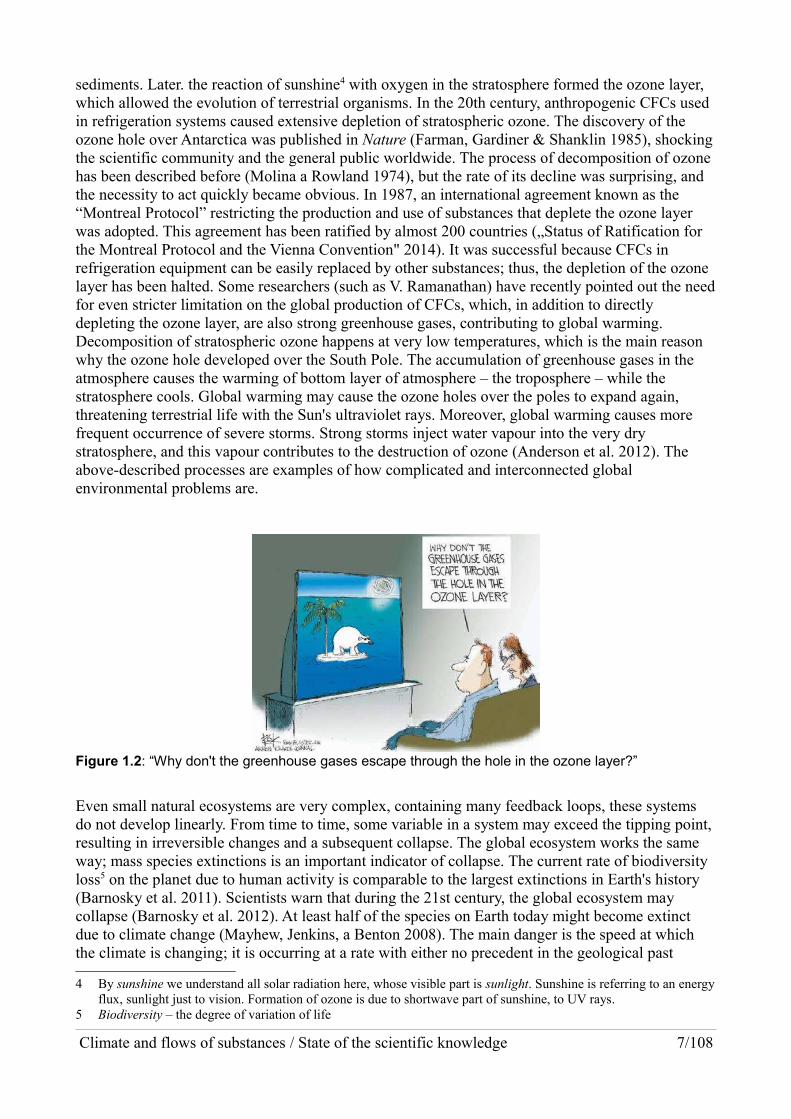
Figure 1.2: “Why don't the greenhouse gases escape through the hole in the ozone layer?”

Even small natural ecosystems are very complex, containing many feedback loops, these systems do not develop linearly. From time to time, some variable in a system may exceed the tipping point, resulting in irreversible changes and a subsequent collapse. The global ecosystem works the same way; mass species extinctions is an important indicator of collapse. The current rate of biodiversity loss5 on the planet due to human activity is comparable to the largest extinctions in Earth's history (Barnosky et al. 2011). Scientists warn that during the 21st century, the global ecosystem may collapse (Barnosky et al. 2012). At least half of the species on Earth today might become extinct due to climate change (Mayhew, Jenkins, a Benton 2008). The main danger is the speed at which the climate is changing; it is occurring at a rate with either no precedent in the geological past

4 By sunshine we understand all solar radiation here, whose visible part is sunlight. Sunshine is referring to an energyflux, sunlight just to vision. Formation of ozone is due to shortwave part of sunshine, to UV rays.

5 Biodiversity – the degree of variation of life

Climate and flows of substances / State of the scientific knowledge 7/108

(Kump 2011) or perhaps just one 56 Ma ago (Wright a Schaller 2013), starting the Paleocene-Eocene Thermal Maximum (PETM).

Anthropogenic global warming is beginning to trigger positive climate feedback loops, such as melting of Arctic sea ice and permafrost making the Earth to absorb more sunshine, or perhaps eventhawing of methane hydrates on Siberian shelf. In principle, the sum of such warming feedbacks could be even stronger than the primary anthropogenic impulse that initiated them. If a critical limit is exceeded, the climate system could go from being in a “warm” state to a “hot” one. The critical limit may be as low as a sustained atmospheric CO2 concentration over 350 ppm, a level which has been exceeded quarter a century ago (Hansen et al. 2008). If the fears of scientists come true, and the end of the 21st century sees a global temperature increase of 6 ºC, conditions on Earth will return to those that prevailed 40 million years ago. People have been walking the Earth for only 200,000 years6, so any ideas about humankind possibly adapting to such conditions are purely speculative. Although scientists' climate models usually just go up to 2100, such extreme global warming enhanced by feedbacks would continue further on in the coming centuries, together with rapid species extinction and diminishing habitability of Earth for humans. Such global warming is a threat comparable to the asteroid collisions and giant volcanic events in the Earth's past that played a significant role in previous extinctions. But even returning to 350 ppm and limiting global warming to below 2 K will not stop further sea level rise in the coming centuries.

At the beginning of the 20th century, global temperature increases were due to an increase in solar radiation and the diminished occurrence of large volcanic eruptions, but the effect of anthropogenic greenhouse gases was beginning to play a role too. When coal is burned, it emits not just CO2, but also pollutants as well, including sulphur oxides, which scatter solar radiation. When there is a greatamount of sulphur in the atmosphere, less sunshine can penetrate it and reach the Earth's surface, which is therefore less heated. The development of industry after World War 2 was accompanied by sulphur emissions produced by combusting coal. Sulphur oxides in the atmosphere contributed to a decline in global temperatures during this period,7 although concentrations of greenhouse gases increased significantly. The acid rains that damaged forests throughout the world were another sign of sulphur pollution. (The mountains in northwest of Bohemia were particularly affected.) In the 1970s, desulfurization equipment was installed in coal-fired power plants in Europe and the USA to stop this damage. Aerosols have a tropospheric lifetime of just a few weeks at most, while much CO2 lasts for centuries and millenia (Archer & Brovkin 2008). Once aerosols were cleared from the atmosphere, the increasing greenhouse effect began to prevail and global temperature started to rise again. Yet even today, the human addition to the greenhouse effect is masked by sulphurous aerosols from Asia, mainly from China, which is feeding its economic boom with more and more non-desulfurised coal plants (Kaufmann et al. 2011).

The first decade of the 21st century has been called a “decade of extremes” by scientists, due to the frequent occurrence and intensity of extreme events such as floods, droughts, heat waves and forest fires (Coumou a Rahmstorf 2012). Consistent with predictions, extreme events have become more common; in some cases, unprecedented extremes have been recorded. This trend will continue due to further global warming. Extreme weather events will increasingly cause economic damage and will make producing enough food to feed a growing population more and more difficult. Threat of disruption of natural ecosystems, such as from disturbances like deforestation, fires and droughts in Amazon rainforest, is serious (Davidson et al. 2012). The climate change that has started with the industrial era is significant in terms of the Holocene, yet it is still small compared to what awaits us in the coming decades.

6 The genus Homo is estimated to have appeared about 2.3 million years ago. The species Homo sapiens is 200,000years old and is the only living species of the genus Homo. To describe modern man, the subspecies Homo sapienssapiens is used, which evolved only 120,000 years ago at the beginning of the previous (Eem) interglacial.

7 The other factor in a break in temperature rise could be a negative phase of Pacific Decadal Oscillation, which seems to be favourable to more heat flux into ocean depths and less warming of its surface and atmosphere.

Climate and flows of substances / State of the scientific knowledge 8/108

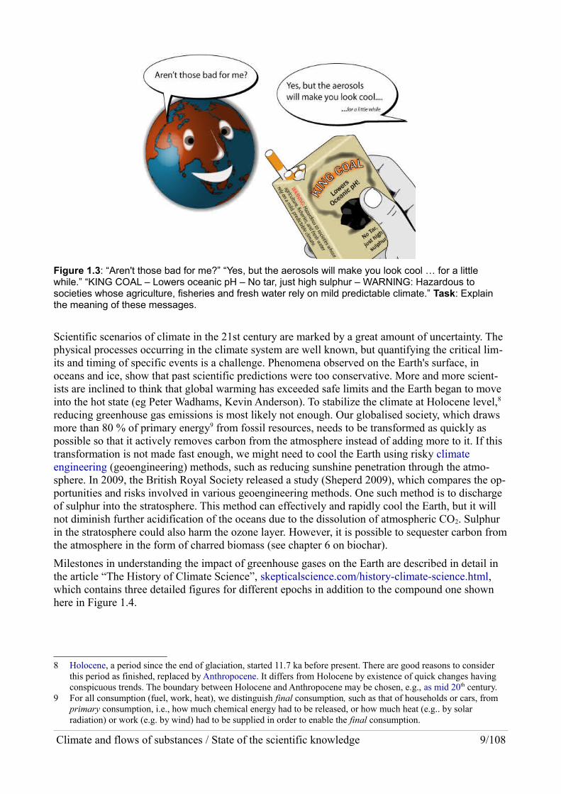
Figure 1.3: “Aren't those bad for me?” “Yes, but the aerosols will make you look cool … for a little while.” “KING COAL – Lowers oceanic pH – No tar, just high sulphur – WARNING: Hazardous to societies whose agriculture, fisheries and fresh water rely on mild predictable climate.” Task: Explain the meaning of these messages.

Scientific scenarios of climate in the 21st century are marked by a great amount of uncertainty. The physical processes occurring in the climate system are well known, but quantifying the critical lim-its and timing of specific events is a challenge. Phenomena observed on the Earth's surface, in oceans and ice, show that past scientific predictions were too conservative. More and more scient-ists are inclined to think that global warming has exceeded safe limits and the Earth began to move into the hot state (eg Peter Wadhams, Kevin Anderson). To stabilize the climate at Holocene level,8 reducing greenhouse gas emissions is most likely not enough. Our globalised society, which draws more than 80 % of primary energy9 from fossil resources, needs to be transformed as quickly as possible so that it actively removes carbon from the atmosphere instead of adding more to it. If this transformation is not made fast enough, we might need to cool the Earth using risky climate engineering (geoengineering) methods, such as reducing sunshine penetration through the atmo-sphere. In 2009, the British Royal Society released a study (Sheperd 2009), which compares the op-portunities and risks involved in various geoengineering methods. One such method is to discharge of sulphur into the stratosphere. This method can effectively and rapidly cool the Earth, but it will not diminish further acidification of the oceans due to the dissolution of atmospheric CO2. Sulphur in the stratosphere could also harm the ozone layer. However, it is possible to sequester carbon fromthe atmosphere in the form of charred biomass (see chapter 6 on biochar).

Milestones in understanding the impact of greenhouse gases on the Earth are described in detail in the article “The History of Climate Science”, skepticalscience.com/history-climate-science.html, which contains three detailed figures for different epochs in addition to the compound one shown here in Figure 1.4.

8 Holocene, a period since the end of glaciation, started 11.7 ka before present. There are good reasons to consider this period as finished, replaced by Anthropocene. It differs from Holocene by existence of quick changes having conspicuous trends. The boundary between Holocene and Anthropocene may be chosen, e.g., as mid 20th century.

9 For all consumption (fuel, work, heat), we distinguish final consumption, such as that of households or cars, from primary consumption, i.e., how much chemical energy had to be released, or how much heat (e.g.. by solar radiation) or work (e.g. by wind) had to be supplied in order to enable the final consumption.

Climate and flows of substances / State of the scientific knowledge 9/108

Climate and flows of substances / State of the scientific knowledge 10/108

Figure 1.4: Milestones in scientific understanding of what controls the temperature of Earth surface.

2 Why is climate changing and how to face itClimate, in the narrow sense, is weather statistics of all kinds (for details see chapter Glossary). This of course varies with daily cycle, as the sun warms the Earth's surface during the day and as the surface cools overnight. And in the annual cycle, as the duration and intensity of isolation changes.

Figure 2.1: An indirect indicator of insolation is the output of a photovoltaic system in Hostětín. The first 25 months of its existence are shown, mainly years 2009 (green) and 2010 (yellow; December 2008, when the first half of the power plant began operation, is orange). Insolation depends not just on the solar path over the sky, but on clouds too (see the graphs from the system online).

A statistics comprising one full year is, however, not so much changing from one year to other and the variation of such annual climates does not show any regularity. Take, for example, the average temperature in a particular year. It can be anomalously high in a region thousands of kilometres large, while it is anomalously low in another region. In layman's terms, this is the result of which way the wind was blowing and how cloudy it was here or there. This is a matter of course for everybody. More surprisingly, even the average surface temperature of Earth as a whole in a particular year may be a tenth of a kelvin (kelvin = degree Celsius) higher or lower than in the previous year. How is this possible when the sun shines almost always the same? In this case, it is not a matter of chaotic wind patterns, which carry heat from one region to other but cannot affect the global average this way. Instead, it is the solar heat that penetrates either a bit more into the depths of the ocean or a bit less, being more readily released from ocean surface into the air. Whether such storage or release of heat prevails, that depends on currents within the whole volume of the oceans. If the climate is in El Niño state, the surface of the eastern tropical Pacific and the air over it heat up, during La Niña episodes, deep ocean waters warm and the surface cools, cooling theair as well. Another variation of annual temperature anomalies is caused by changes in cloud cover, and thus in the Earth's albedo (see p. 52) and the portion of greenhouse effect caused by clouds. For more about the greenhouse effect, see Glossary and Diagram of the greenhouse effect and sources of greenhouse gases from human activities in the Appendix.

When much longer time intervals are used – in climatology, three-decade periods most commonly –the climate should remain very stable, little changing from one period to the next one, as oscillations of ocean currents have shorter time scales. And it used to be rather stable for almost 12,000 years, throughout the Holocene. At least in terms of global temperature anomaly. But what about earlier in the Quaternary, during the Pleistocene (see en.wikipedia.org/wiki/Ice_age)?

Climate and flows of substances / Why is climate changing and how to face it 11/108

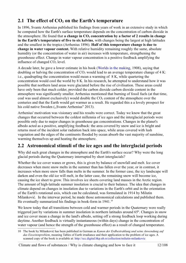
2.1 The effect of CO2 on the Earth's temperatureIn 1896, Svante Arrhenius published his findings from years of work in an extensive study in whichhe computed how the Earth's surface temperature depends on the concentration of carbon dioxide inthe atmosphere. He found that a change in CO2 concentration by a factor of 2 results in change in the Earth's temperature of five to six kelvins, with changes being the largest at high latitudes and the smallest in the tropics (Arrhenius 1896). Half of this temperature change is due to change in water vapour content. With relative humidity remaining roughly the same, absolute humidity (or the concentration of water in air) increases with temperature, strengthening the greenhouse effect. Change in water vapour concentration is a positive feedback amplifying the influence of changed CO2 level.

A decade later, he gave a lower estimate in his book (Worlds in the making, 1908), saying that doubling or halving the concentration of CO2 would lead to an average temperature change of 4 K: i.e., quadrupling the concentration would mean a warming of 8 K, while quartering the concentration would cool the world by 8 K. In his research, he attempted to understand how it was possible that northern land areas were glaciated before the rise of civilisation. These areas could have only been that much colder, provided the carbon dioxide carbon dioxide content in the atmosphere was significantly smaller. Arrhenius mentioned that burning of fossil fuels (at that time, coal was used almost exclusively) would double the CO2 content of the atmosphere over the centuries and that the Earth would get warmer as a result. He regarded this a a lovely prospect for his cold native Sweden („Svante Arrhenius" 2013).

Arrhenius' motivation was visionary and his results were correct. Today we know that the great changes that occurred between the coldest millennia of ice ages and the interglacial periods were possible only due to major changes in greenhouse gas concentrations. Changes in the planet's albedo acted as a positive, amplifying feedback: the area covered by snow and ice is bright and returns most of the incident solar radiation back into space, while areas covered with lush vegetation and the edges of the continents flooded by ocean absorb the vast majority of sunshine, warming themselves up and heating the atmosphere.

2.2 Astronomical stimuli of the ice ages and the interglacial periodsWhy did such great changes in the atmosphere and the Earth's surface occur? Why were the long glacial periods during the Quaternary interrupted by short interglacials?

Whether the ice cover wanes or grows, this is given by balance of snowfall and melt. Ice cover decreases when more snow melts in the summer than has fallen over the year, or in contrast, it increases when more snow falls than melts in the summer. In the former case, the icy landscape willdarken and even the old ice will melt, in the latter case, the remaining snow will become ice, causing the ice sheet to grow. This involves ice sheets covering land masses in the Arctic region. The amount of high-latitude summer insolation is crucial to their balance. The idea that changes in climate depend on changes in insolation due to variations in the Earth's orbit and in the orientation of the Earth's rotational axis, which can be calculated, was formulated in 1914 by Milutin Milanković. In the interwar period, he made those astronomical calculations and published them. He eventually summarized his findings in book-form in 1941.10

We know today that all transitions between cold and warmer periods in the Quaternary were really triggered just by variations in summer insolation in northern latitudes around 65º. Changes in snow and ice cover mean a change in the land's albedo, setting off a strong feedback loop working during daytime. Another feedback is virtually instantaneous (within days) change in the concentration of water vapour (and hence the strength of the greenhouse effect) as a result of changed temperature.

10 The book by Milanković has been published in German as Kanon der Erdbestrahlung und seine Anwendung auf das Eiszeitenproblem, meaning Tables of Earth irradiance and their application to the problem of ice ages. A scanned copy of the book is available at: http://scc.digital.bkp.nb.rs/collection/milutin-milankovic

Climate and flows of substances / Why is climate changing and how to face it 12/108

The temperature persistently altered that way led to a change of the concentration of the three naturally occurring long-lived greenhouse gases over time: of carbon dioxide, methane, and nitrous oxide.

When glacial had been warming to interglacial, carbon dioxide was released from the seas, as warmer water cannot hold as much of it (think of what happens to a fizzy drink or beer as it gets warmer). Methane was released from the warming soils and seabed of the Arctic and newly produced due to increased microbial activity in soils or wetlands; this production concerns also nitrous oxide. Elevated concentrations of these three greenhouse gases caused temperature changes not only in high northern latitudes during summer, but over the entire planet throughout the whole year. Global temperature changes then led to changes of albedo in the high southern latitudes. At both hemispheres, albedo decreased even in lower latitudes. All these changes greatly amplified the the impact of the initial astronomical trigger, the increased summer insolation.

Milanković was absolutely right that the impetus for change lies outside the climate system, being entirely astronomical in nature. He just did not realize that in order for insolation changes to have a global effect, a strong (positive) feedback, the increased greenhouse effect is necessary. He would certainly be pleased to discover that findings on the timing of past climate changes acquired from boreholes drilled in the ice sheets of Greenland and Antarctica and from the analysis of deep see sediments align perfectly with high-latitude insolation rises or decreases, according to his wise physical idea. Of course, the insolation of upper layers of the atmosphere in high northern latitudes is now calculated more accurately, by numerical modelling using computers. It can be said that today, climate changes in the Quaternary are understood quite well.

You may often encounter the term “Milanković cycles” – but these cycles concern three variables, namely the ecliptic longitude of perihelion, the inclination of the Earth's axis and the eccentricity of Earth's orbit. What really matters, however, is their combination resulting in changing irradiance of high northern latitudes in spring and summer. Unlike Earth's insolation as a whole, which does not change through millenia, high latitude summer irradiance varies significantly over the course of thousands and tens of thousands of years. The variation amounts to tens of watts per square metre, see Figure 2.2.

Maximum levels of irradiance lead to loss of snow and the volume of ice masses in the high northern latitudes, a decrease in albedo, warming and an increase in the concentration of carbon dioxide. Minimum levels put the opposite process in motion. But such whether such an astronomically initiated process leads to a significant change, that depends on the state of the climate system and its dynamics as well.

It turns out that the warming at the end of Pleistocene began by the thawing of the continental ice, resulting in covering the North Atlantic by less salty water, which suppressed the thermohaline circulation11 that supplies heat from southern hemisphere to the northern latitudes. This increased the temperature of the Southern Ocean. Water flow from depths of the Southern Ocean to its surfaceincreased too, as models show. This deep water released carbon dioxide. Increase of its content in the air then led to large warming of the whole planet (Shakun et al. 2012) (Tzedakis et al. 2012) („RealClimate: Unlocking the secrets to ending an Ice Age" 2012) (“CO2 Lags Temperature – WhatDoes It Mean?” 2012) (Meckler et al. 2013) (He et al. 2013).

Ice ages usually begin and end when the difference between maximum and minimum irradiance of high latitudes is particularly large. However, variation with a relatively small amplitude started and ended the long warm period 400 thousand years ago. The current warm period, the post-glacial started also with a swing of insolation which was not particularly large.

11 As the name suggests, this motion occurs due to changes in temperature and salinity, which cause density anomalies. See en.wikipedia.org/wiki/Thermohaline_circulation.

Climate and flows of substances / Why is climate changing and how to face it 13/108

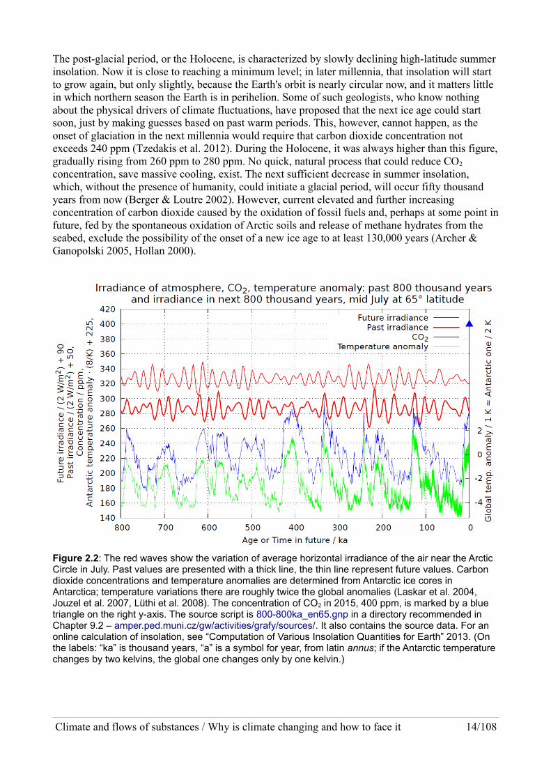
The post-glacial period, or the Holocene, is characterized by slowly declining high-latitude summer insolation. Now it is close to reaching a minimum level; in later millennia, that insolation will start to grow again, but only slightly, because the Earth's orbit is nearly circular now, and it matters little in which northern season the Earth is in perihelion. Some of such geologists, who know nothing about the physical drivers of climate fluctuations, have proposed that the next ice age could start soon, just by making guesses based on past warm periods. This, however, cannot happen, as the onset of glaciation in the next millennia would require that carbon dioxide concentration not exceeds 240 ppm (Tzedakis et al. 2012). During the Holocene, it was always higher than this figure,gradually rising from 260 ppm to 280 ppm. No quick, natural process that could reduce CO2 concentration, save massive cooling, exist. The next sufficient decrease in summer insolation, which, without the presence of humanity, could initiate a glacial period, will occur fifty thousand years from now (Berger & Loutre 2002). However, current elevated and further increasing concentration of carbon dioxide caused by the oxidation of fossil fuels and, perhaps at some point infuture, fed by the spontaneous oxidation of Arctic soils and release of methane hydrates from the seabed, exclude the possibility of the onset of a new ice age to at least 130,000 years (Archer & Ganopolski 2005, Hollan 2000).

Figure 2.2: The red waves show the variation of average horizontal irradiance of the air near the Arctic Circle in July. Past values are presented with a thick line, the thin line represent future values. Carbon dioxide concentrations and temperature anomalies are determined from Antarctic ice cores in Antarctica; temperature variations there are roughly twice the global anomalies (Laskar et al. 2004, Jouzel et al. 2007, Lüthi et al. 2008). The concentration of CO2 in 2015, 400 ppm, is marked by a blue triangle on the right y-axis. The source script is 800-800ka_en65.gnp in a directory recommended in Chapter 9.2 – amper.ped.muni.cz/gw/activities/grafy/sources/. It also contains the source data. For an online calculation of insolation, see “Computation of Various Insolation Quantities for Earth” 2013. (On the labels: “ka” is thousand years, “a” is a symbol for year, from latin annus; if the Antarctic temperature changes by two kelvins, the global one changes only by one kelvin.)

Climate and flows of substances / Why is climate changing and how to face it 14/108

Milankovitch theory explains well the alternation of ice ages and interglacials over the last three million years. Nevertheless, it has little or no bearing for future climate developments, because:

To initiate a new glaciation, the orbit of the Earth has to be very eccentric, and the northern hemisphere has to be inclined to Sun when Earth is at aphelion. Cool summers in the northern hemisphere then allow the accumulation of ice. Since the Earth orbit is close to being perfectly circular now, this mechanism is “switched off ”.

The condition under which glaciation can start is a combination of summer irradiance and the concentration of greenhouse gases. People burning fossil fuels have changed the atmosphere so much that glaciation due to changes in summer insolation is out of the question for at least the next 130,000 years.

The current global warming has no analogy during most of the Tertiary period, the nearest events itcan be compared with are the boundary Paleocene-Eocene 56 million years ago and the transition from Permian to Triassic 151 million years ago.

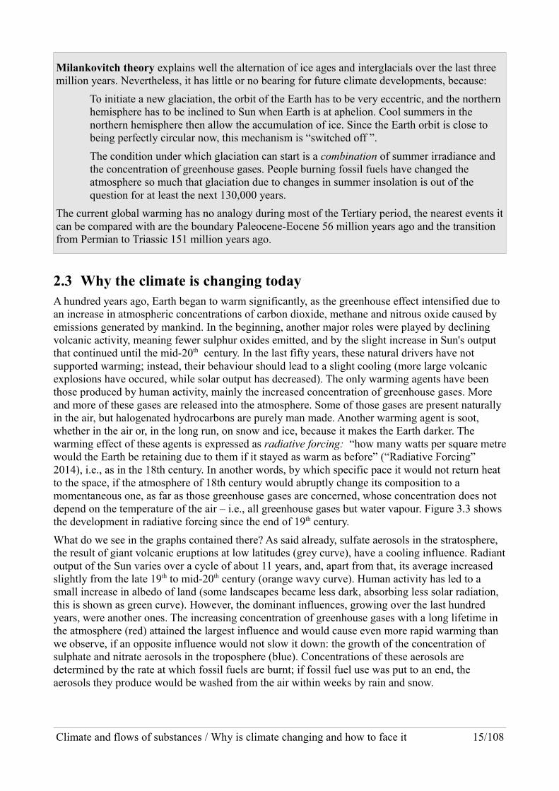
2.3 Why the climate is changing todayA hundred years ago, Earth began to warm significantly, as the greenhouse effect intensified due to an increase in atmospheric concentrations of carbon dioxide, methane and nitrous oxide caused by emissions generated by mankind. In the beginning, another major roles were played by declining volcanic activity, meaning fewer sulphur oxides emitted, and by the slight increase in Sun's output that continued until the mid-20th century. In the last fifty years, these natural drivers have not supported warming; instead, their behaviour should lead to a slight cooling (more large volcanic explosions have occured, while solar output has decreased). The only warming agents have been those produced by human activity, mainly the increased concentration of greenhouse gases. More and more of these gases are released into the atmosphere. Some of those gases are present naturally in the air, but halogenated hydrocarbons are purely man made. Another warming agent is soot, whether in the air or, in the long run, on snow and ice, because it makes the Earth darker. The warming effect of these agents is expressed as radiative forcing: “how many watts per square metrewould the Earth be retaining due to them if it stayed as warm as before” (“Radiative Forcing” 2014), i.e., as in the 18th century. In another words, by which specific pace it would not return heat to the space, if the atmosphere of 18th century would abruptly change its composition to a momentaneous one, as far as those greenhouse gases are concerned, whose concentration does not depend on the temperature of the air – i.e., all greenhouse gases but water vapour. Figure 3.3 shows the development in radiative forcing since the end of 19th century.

What do we see in the graphs contained there? As said already, sulfate aerosols in the stratosphere, the result of giant volcanic eruptions at low latitudes (grey curve), have a cooling influence. Radiantoutput of the Sun varies over a cycle of about 11 years, and, apart from that, its average increased slightly from the late 19th to mid-20th century (orange wavy curve). Human activity has led to a small increase in albedo of land (some landscapes became less dark, absorbing less solar radiation, this is shown as green curve). However, the dominant influences, growing over the last hundred years, were another ones. The increasing concentration of greenhouse gases with a long lifetime in the atmosphere (red) attained the largest influence and would cause even more rapid warming than we observe, if an opposite influence would not slow it down: the growth of the concentration of sulphate and nitrate aerosols in the troposphere (blue). Concentrations of these aerosols are determined by the rate at which fossil fuels are burnt; if fossil fuel use was put to an end, the aerosols they produce would be washed from the air within weeks by rain and snow.

Climate and flows of substances / Why is climate changing and how to face it 15/108

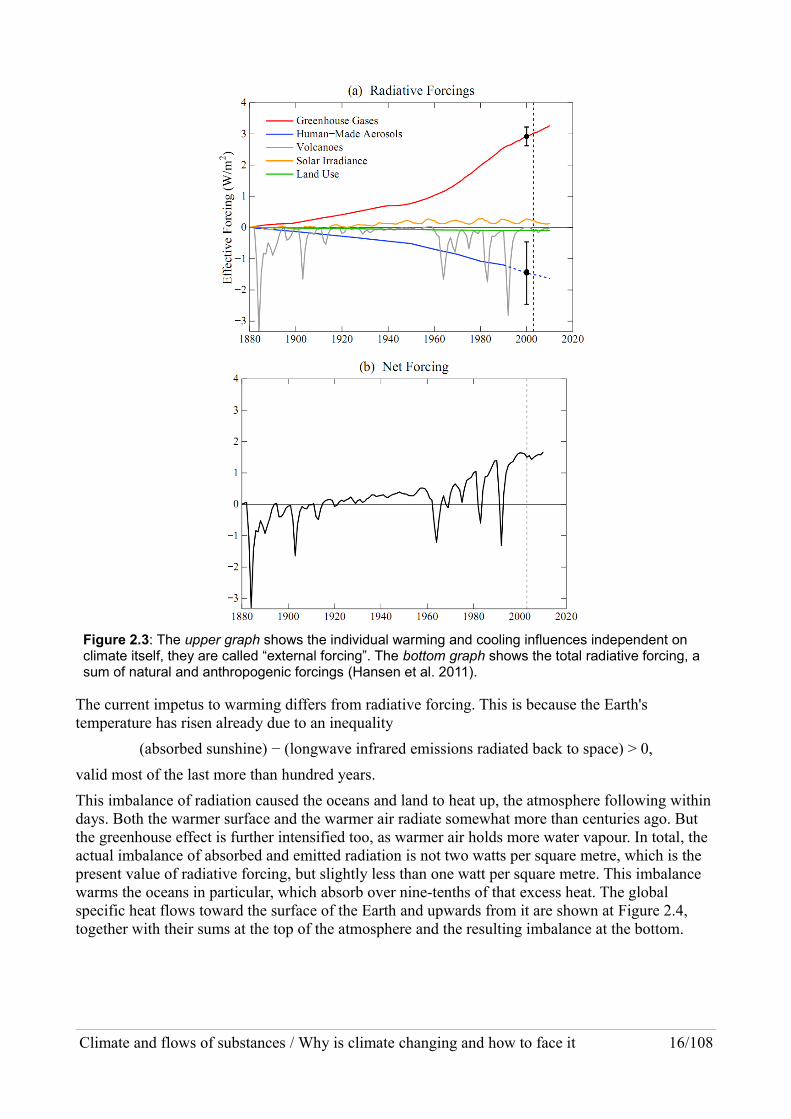
Figure 2.3: The upper graph shows the individual warming and cooling influences independent on climate itself, they are called “external forcing”. The bottom graph shows the total radiative forcing, a sum of natural and anthropogenic forcings (Hansen et al. 2011).

The current impetus to warming differs from radiative forcing. This is because the Earth's temperature has risen already due to an inequality

(absorbed sunshine) − (longwave infrared emissions radiated back to space) > 0,

valid most of the last more than hundred years.

This imbalance of radiation caused the oceans and land to heat up, the atmosphere following within days. Both the warmer surface and the warmer air radiate somewhat more than centuries ago. But the greenhouse effect is further intensified too, as warmer air holds more water vapour. In total, the actual imbalance of absorbed and emitted radiation is not two watts per square metre, which is the present value of radiative forcing, but slightly less than one watt per square metre. This imbalance warms the oceans in particular, which absorb over nine-tenths of that excess heat. The global specific heat flows toward the surface of the Earth and upwards from it are shown at Figure 2.4, together with their sums at the top of the atmosphere and the resulting imbalance at the bottom.

Climate and flows of substances / Why is climate changing and how to face it 16/108

Figure 2.4: Energy fluxes through Earth atmosphere taken globally, for 2000-2005 (Trenberth a Fasullo 2011).

Global warming caused by the disturbance of the previous radiative balance of the Earth is far from being spatially uniform. High northern latitudes in the Arctic are warming most rapidly. This is happening for two reasons. The air there has always been so cold (and still is) that it contains little water vapour, so increases in those greenhouse gases that are not dependent upon temperature independent and that are almost perfectly mixed in the troposphere have a more noticable impact there. Even more important though is the amplifying feedback: warming shrinks snow and ice coverof the sea and land, making these areas darker and thus absorbing more solar radiation. This positive feedback is made even stronger by black carbon (e.g., as core of soot particles) from diesel engines and other combustion processes. Black carbon decreases albedo of areas where the “eternal” snow and ice still remains, such as on the Greenland ice sheet.

In spite of that, the greatest Arctic warming is observed during the polar night. Not only that the better-insulating atmosphere does not let the land and sea cool down so quickly and strongly as decades before. The warmer ocean remains ice-free much longer into winter, preventing temperature fall of more than a couple kelvins below freezing point of sea water.

What we should devote our attention to primarily, is, of course, the dominant driver of warming of the Earth: rising concentration of carbon dioxide. The flow of carbon into the atmosphere caused directly by mankind, from fossil fuels, cement production, soil degradation (loss of organic matter, including humus) and deforestation is already ten billion tons per year (10 Gt/a) and rising. In comparison, the geological flow of carbon from sediments into the atmosphere, resulting from the subduction of the ocean floor and subsequent volcanic activity, is one hundred times smaller. An overview of these processes is presented in Figure 2, How people add carbon to the atmosphere and how to stop it, in the Appendix.

Climate and flows of substances / Why is climate changing and how to face it 17/108

The increase of carbon dioxide in the atmosphere (depicted by the Keeling curve) and the corresponding decrease of the oxygen content is plotted in Figure 7.2 in the chapter “A model of thebiosphere”. Commentary on it see in chapter 2.3.1 of the first volume of AR4. Extraordinarily impressive animation of CO2 concentration changes over time see (please!) at www.esrl.noaa.gov/gmd/ccgg/trends/history.html. (It's becoming more and more common that people call the Keeling curve the most important graph of all times – everybody should know it.)

Figure 2.5: The upper graph shows the global temperature anomalies of near-ground air temperature over land and of ocean surface temperature. Its bottom edge is marked by episodes of great volcanic eruptions which created a large layer of aerosols in the stratosphere. Blue bars represent estimates of 95 % confidence interval for comparing nearby years. The Nino Index shown in the following graph is based on detrended temperature in the Niño 3.4 region in the eastern tropical Pacific (Philander 2006). It is apparent that volcanic eruptions and negative Niño index values result in years that are globally colder. Positive index values lead to warmer years. The four anomaly maps show the seasons, from December 2011 to November 2012. The baseline period to which the temperature anomalies refer is the average for the years 1951-1980 (Hansen, Sato, a Ruedy 2013). (Index Niño 3.4 is the temperatureanomaly / 1 K in central to eastern equatorial Pacific, see link.)

2.4 How the climate changes… it's not just average temperaturesChanges in the average temperature of the Earth's surface (or in the case of continents, of the air above them at a height of 2 m) is the simplest indicator of climate change. However, as regards

Climate and flows of substances / Why is climate changing and how to face it 18/108

the imbalance between heat absorption and emission by the Earth as a whole, the increase of ocean temperatures is the critical indicator.

Figure 2.6: The upper graph classifies years according to a composite index describing the changing conditions on the ENSO index as positive, neutral and negative. Years in which global surface temperature anomaly decreased due to volcanic eruptions of El Chichon (1983-1985) and Mount Pinatubo (1992-1994) are marked as triangles. The forty-year growth trend is 0.15 to 0.16 kelvin per decade for all 3 lines (Nuccitelli 2012). For a more recent animated version of this graph see http://www.skepticalscience.com/graphics.php?g=67.

The lower graph shows the increase in the enthalpy of the oceans. The black curve describes the depths down to two kilometres, while the red one only covers the upper 700 m of the ocean. Both curves represent five-year running averages. In this depiction, the growth of enthalpy (and of ocean temperatures) would be monotonous, as long as there are no giant volcanic eruptions (US Department of Commerce 2013).

Task: Calculate the minimum possible imbalance between absorption and output of heat by the Earth averaged over the last twenty years. In reality, the imbalance would be larger, as the graph neglects thewarming of the oceans at depths below 2 km, as well as the heating of the continents, the atmosphere and melting of ice. Express the result also per unit area per second, in watts per square metre.

Climate and flows of substances / Why is climate changing and how to face it 19/108

The growth of the global (near-ground + sea surface) temperature anomaly is not uniform over time periods less than twenty years. This is due mainly to irregular periods of El Niño (when the Niño 3.4 index os over 0.5) or La Niña (a situation when the index is below −0.5) states of the climate system. But if we sort individual years into 3 groups according to strongly positive, neutral or strongly negative index values, then the warming of the Earth's surface is rather even in each group.However, the most telling data are not from the surface, but from the upper half of the volume of the oceans. For the bottom half – the average depth of the oceans is 4 km – data are still missing; however, from summer 2014, the invaluable project ARGO started to provide measurements down to 6 km depth (“Deep ARGO”).

You can often meet an argument that the early Holocene was warmer than today (an extreme example of such disinformation see http://www.skepticalscience.com/10000-years-warmer.htm). In the Central European geological tradition, this warm period referred to as the “Holocene Climate Optimum” – with the implication that developments are actually welcome. Global temperature anomaly throughout the Holocene, however, never exceeded the current anomaly, and its changes took place at up to two orders of magnitude slower then temperatures are currently rising. This is depicted in Figure 2.7.

Figure 2.7: Reconstruction of global temperature variations during the Holocene and the Anthropocene.Even for the last century indirect (proxy) indicators are employed; of course, they are in good agreement with measured temperatures. Elevated and rising concentrations of greenhouse gases will lead inevitably to further warming; current emission trends, if continued, would lead to warming of up to four kelvin this century. The graph (Romm 2013) is based on a temperature reconstruction published in Science (Marcott et al. 2013).

For human civilization and nature, changes in extremes are more important than changes of averages, whether this concerns temperature, precipitation, evaporation or wind. Extremes of both types (values unusually high or low) limit the habitability of various regions of the Earth. As average temperatures continue to grow, is can be expected that the number of cases where temperature in some area is extremely high rises too. However, the frequency of such hot extremes increases even faster, see Figure 2.8. This implies that temperatures are not only rising, but they are also becoming much more variable.

Climate and flows of substances / Why is climate changing and how to face it 20/108

Extremely high temperatures lasting a month or more present us with unprecedented challenges. If accompanied by a decrease in precipitation, then a drought results, worsened by a warmer air sucking more water from the soil and plants. Take, for example, the drought that affected the centralUSA in spring 2012 (see Figure 2.5). It generally holds true that with continued warming both highand low extremes in the water cycle grow. Dry areas are becoming drier; areas with plenty of precipitation are receiving more of it. Simple reasons for this development are as follows. Warmer air can transport more water vapour from the oceans. However, if the air has dried already by precipitation and warmed again, it sucks moisture more quickly from the land. And again, not just annual precipitation and evaporation are affected, but seasonal extremes are amplified as well – wet periods become wetter, as dry periods become drier. These changes are devastating for agriculture. In poor countries, where people are totally dependent on what they can grow themselves, this often means that people complete lose their livelihood and subsequently migrate to cities or even neighbouring countries. Current drought severity as well as projections for the future are shown in Figure 2.9. While Scandinavia will be wetter, cereal-producing areas of North Americaand the Mediterranean are already seriously affected. The general reason for the expansion and intensification of the subtropical drought belt is a growth in air rising from the tropics; after precipitation falls from it back to tropical latitudes, the air returns down to the surface at higher latitudes with very low relative humidity.

Figure 2.8: The frequency of occurrence of different average summer temperatures (i.e., average for the months of June, July and August) at six thousand stations in the northern hemisphere. The horizontal axis represents the deviation from the long-term average for the years 1951-1980, in units of “standard deviation” applicable to that station. In this first, reference period, summer temperature anomalies were distributed normally; cold, normal and warm summers, represented by different colours, each make about one third of cases. Summers with average temperatures exceeding three standard deviations occurred, in accordance with the course of the normal distribution, once per one thousand cases. In the following decades, the occurrence of hot summers climbed and that of cold ones waned. In this millennium, the number of cases where the summer temperature exceeded the average of the reference period by “three sigma”, or three standard deviations of the reference frequency distribution, amounted to almost ten percent. In other words, extremely hot three-month summer periods, which occurred just on one tenth of a percent of the area of the Northern Hemisphere's land mass, are now found in an area one hundred times larger (Hansen, Sato, a Ruedy 2013). (In Czech, see also a text from 2012 at http://amper.ped.muni.cz/gw/hansen).

Climate and flows of substances / Why is climate changing and how to face it 21/108

Figure 2.9: Drought severity index. Calculated on the basis of surface temperature, precipitation, relative humidity, net radiation and wind speed, as an average of 22 models assuming development scenario SRES A1B. Drought is a deviation from the former conditions in the region, index values of -4 (red) and less indicate extreme drought. (Dai 2010)

The rate of warming over the last four decades is, and also will be until at least the mid-21st century, at least ten times higher than at any time in the last 55 million years. This, among other things, has caused ocean temperatures to lag behind land surface temperatures; greater temperature contrasts can produce unusually strong storms. A new phenomenon, which has not occurred in at least the past five thousand years, is a much warmer Arctic ocean, in which the majority of ice cover breaks up during summer. The ocean then becomes a massive source of heat and water vapour until it freezes again (later in winter than decades ago). Arcticwarming is most pronounced in winter and spring, when it leads to early snow melt. This darker Arctic is then heated more by the sun. The reduced temperature contrast between the Arctic and temperate latitudes slows down the jet stream (en.wikipedia.org/wiki/Jet_stream) around the Arctic in the upper troposphere. Moreover, the stream meanders more to the north and south, and these so-called Rossby waves move more slowly to the east than in the past. As a result, cold air can penetrate far south, or vice versa warm air can spread northwards. Prolonged heavy rainfalls or hot and dry spells may be a consequence (Francis a Vavrus 2012). The much warmer, darker and further warming Arctic is fundamentally changing weather patterns in the zone where majority of mankind lives, which enjoyed a mild climate during the Holocene.

One of consequences of a warmer ocean surface in these areas are heavy snowfalls, affecting the eastern coast of the United States and the European Union, even though snowfall annual have diminished over the years. Greater evaporation and warmer air capable to hold more water vapour open the door to greater precipitation and at temperatures just below zero, it means snow. Therefore, during the winter half-year (October to March) snow will of course continue to fall in mid-latitudes, even if less often, throughout the 21st century.

2.5 Can we stop warming?Technically, the answer to this question is yes. Provided the use of fossil fuels is phased out by mid-century, warming might stop... Increasing exploitation of fossil fuels, however, has been bound to GDP growth – and without GDP growth and consumption growth, major industrial economies will have serious difficulties leading to social conflicts. Nevertheless, economic

Climate and flows of substances / Why is climate changing and how to face it 22/108

performance can be maintained even if fossil fuel consumption is reduced, as long as there is an abundance of good will and a consensus that investments may only be made in projects that do not increase fossil fuel consumption, if possible reduce it, and, even better, reduce consumption in general.

A typical example of such an investment is regeneration of buildings so that they approach as close to the passive house standard as possible, supplemented by the solar optimization of suitably oriented surfaces of buildings – if they are not fully occupied by windows, then they should be covered by hot water collectors or photovoltaic panels. Even a generous layer of thermal insulation can be designed so that its production demands smaller quantities of oil, natural gas and coal than corresponds to the mass of carbon bound in the very insulating material. This can be achieved by insulating with an appropriate type of biomass, most easily, straw (Haselsteiner et al. 2012). Other investments may minimize the use of car traffic, in favour of walking, cycling, public transportation(preferably powered by electricity), or even to reduce the transport of people and goods in general.

Artificial electric lighting, ever stronger, has been the very symbol of progress since its beginning. But at night, it is deleterious to health (Fonken a Nelson 2011) and its increase brings no more comfort. Night lighting that is no stronger than that used in the nineteenth century can now be achieved extremely cost-effectively by using light emitting diodes. To power them, no large power grid is needed, modest local, renewable sources combined with batteries are enough. The same applies to mobile phones and today's compact computers, which are just a bit heavier. There are several reasons the availability of these two technologies is a precondition for developing countries to escape from poverty. For example, the most effective measure against population explosion is higher rates of female education, and an access to internet and to reading after dusk can boost it a lot.

In practice, unfortunately, the so-called Jevons paradox applies (Missemer 2012), see en.wikipedia.org/wiki/Jevons_paradox, saying that increasing energy efficiency leads (through economic processes) to rapid resource depletion. For example, introduction of “energy-efficient” light sources often leads to stronger or completely unnecessary lighting. People who own fuel-efficient cars tend to drive more often and take longer trips, meaning that fuel consumption is not reduced, but instead, it may even increase (this is called rebound effect). Such consequences can be overcome by making a personal decision not to spend your income on consumption, but instead to donate a good part of it to a reasonable “charity” that supports development of the world towards sustainability. If such attitudes gain in society-wide popularity, then perhaps tax measures that will make consumption more costly, effectively taking money from those who themselves don't allocate it wisely, can be introduced. For a steady decline in consumption, energy efficiency measures have to be combined with a significant and gradually increasing fee levied on all extracted fossil carbon (and, if possible, an order of magnitude larger penalty for methane leaks) – for details see http://www.carbontax.org/. A large proportion of fee collected should be evenly distributed throughout population; people with low levels of consumption will profit, while for others it will be an incentive for introducing technological change or reducing consumption by altering their habits. Distribution of the entire income from the carbon fees to all residents is promoted by Dr. James Hansen, http://www.columbia.edu/~jeh1/ (as in his text from Dec 23, 2014, www.columbia.edu/~jeh1/mailings/2014/20141223_AssuringRealProgress.pdf). (Some Czech translations of his texts see at http://amper.ped.muni.cz/gw/hansen/; Czech texts on economy with declining consumption see p. 73-78 of doctoral thesis Fraňková 2012b and a brochure Fraňková 2012a. We stress the urgency of these approaches being made known even to people who don't study English texts.)

Virtually every country in the world has declared that global warming has to be limited so that it does not exceed two degrees: “no more than 2 K”. But no country yet had entered a path tomake its fair share of necessary changes in society a reality. Although the fact that the UK has

Climate and flows of substances / Why is climate changing and how to face it 23/108

legally bound itsldf to reducing its greenhouse gas emissions by four-fifths till 2050 is pleasing, thisdecrease is not enough for staying below the 2 K mark. Global greenhouse gas emissions are still rising and the rise even accelerates. Local British emissions are falling, but emissions attributable tothe British population are not, considering how much greenhouse gas is released to produce goods imported into Britain. And science has demonstrated that a rise in temperature of 2 K would betoo much, having bad and serious consequences for humankind and the entire biosphere, including a danger that further carbon would begin to be released from the surface layers of Arctic land and from shallow Siberian seabed.

Meeting the “no more than 2 K” goal is possible only through fundamental changes in global politics and the world economy. In principle, it is still possible to keep the warming below 1.5 K (Hansen, Kharecha, et al. 2013). The other important issue is the duration of such elevated temperatures. If emissions fall sufficiently, atmospheric concentrations will go down. If the proportion of CO2 in the atmosphere returns to somewhere below 350 ppm, (see 350.org) then temperatures will decrease instead rise. An even more reliable goal is 333 ppm goal (Ač 2013), see the petition at https://yourclimatechange.org/. Meeting this target may slow down or perhaps even stop the disintegration of the Greenland Ice Sheet. As far as the West Antarctic Ice Sheet is concerned, it seems that at least a partial collapse is inevitable (Rignot et al. 2014) (Joughin, Smith, a Medley 2014), but its pace can be reduced. The final rise in sea levels can still be limited to several metres instead of more than 10 m. In any case, if the warming is to be stopped, most deposits of fossil fuels that are currently being exploited should be abandoned, never mind accessing new ones. Carbon must no longer be released from sediments; instead a new era must begin in which carbon is redeposited from the atmopshere into the biosphere. This can be done through better agricultural and forestry practices. The should include a “new” way of using biomass: not by completely oxidising it (either by burning it, leaving it to spontaneously decompose, or deliberately composting it), but by turning some of the carbon it contains (taken from the atmosphere by photosynthesis) to char, which is incorporated to soil – see the chapter 6 Biochar.

Climate and flows of substances / Why is climate changing and how to face it 24/108

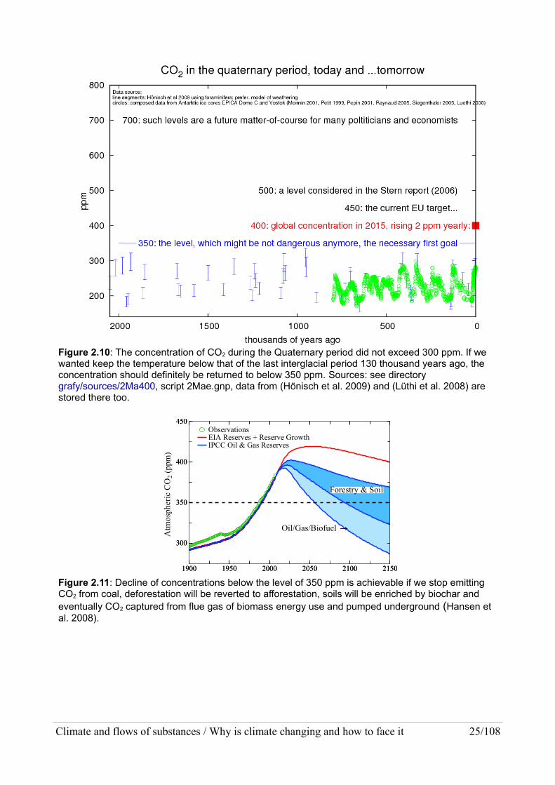
Figure 2.10: The concentration of CO2 during the Quaternary period did not exceed 300 ppm. If we wanted keep the temperature below that of the last interglacial period 130 thousand years ago, the concentration should definitely be returned to below 350 ppm. Sources: see directory grafy/sources/2Ma400, script 2Mae.gnp, data from (Hönisch et al. 2009) and (Lüthi et al. 2008) are stored there too.

1900 1950 2000 2050 2100 2150

300

350

400

450ObservationsEIA Reserves + Reserve GrowthIPCC Oil & Gas Reserves

Atm

osph

eric

CO

2(p

pm)

Forestry & Soil

Oil/Gas/Biofuel →

1900 1950 2000 2050 2100 2150

300

350

400

450

Figure 2.11: Decline of concentrations below the level of 350 ppm is achievable if we stop emitting CO2 from coal, deforestation will be reverted to afforestation, soils will be enriched by biochar and eventually CO2 captured from flue gas of biomass energy use and pumped underground (Hansen et al. 2008).

Climate and flows of substances / Why is climate changing and how to face it 25/108

3 Educating about global climate changeEducation should prepare people for life in a world that is the product of natural and human history. But what will the world look like in 20–30 years? What knowledge and skills will today's students need as adults? In the late 1960s, many people believed that in 2000s travelling to the moon would be common. At that time, development in space travel certainly suggested this would be so, yet nonetheless the last time a human being walked on the Moon was in 1972. At present, technology is progressing at a precipitous rate that has had profound effect on people's daily lives. One can get the feeling that this progress will last forever. People tend to predict the future based on their own experiences, but the world is not linear. There are many examples in history of when the entire world and life as people knew it changed fundamentally over a short period of time (e.g., the Great Depression and the two World Wars). There are good reasons to assume that the world is at such a turning point right now.

Task: Do you see any evidence in favour of this claim or against it? Let's discuss it!

Figure 3.1: Czech text: kindergarten, elementary school, secondary school, university. Author: Jozef “Danglár” Gertli

Advances in information and communication technologies may be fascinating, but although you could easily survive without a “smart phone”, the same cannot be said of not having food and water.The Achilles' heel of our civilization is agriculture, which must be capable to feed a rapidly growingpopulation. If global climate change continues to be an ever more dominant factor influencing changes in the biosphere, it is hard to imagine that our agriculture-based civilization would remain unaffected. Most agricultural production depends on cheap petroleum products, but half of the world's oil reserves have been used up already. What will farmers fuel their tractors with if oil will becomes too expensive for them? We are only a decade and a half into the 21st century and climate change has already repeatedly caused major crop losses; strategic food reserves are rapidly being depleted. City dwellers are used to buy from shelves loaded with cheap food. Will this last forever? If schools are to adequately prepare future generations for life, it is essential that society's expectations are not too at odds with reality.

We do not need a crystal ball to read the future. Scientists are modelling the climate system using powerful supercomputers. Unfortunately, even with all increase in computing power and complexity their Earth system models are far from perfect. Current observations show us that existing models are hardly able to match the reality. The climate system reacts to anthropogenic

Climate and flows of substances / Educating about global climate change 26/108

stimuli faster than projected. Accelerated melting of land-based ice masses, of Arctic sea ice and permafrost, rising sea levels, changes in ecosystems and many other indicators suggest that the climate system is shifting to a never witnessed, hot state faster than predicted by the IPCC report12 from 2007. Scientific research into climate change has advanced considerably in the last decade, and we can expect big changes in the climate system that will need to be taken into account by climate scientists.

It is not only future generations that will have to adapt to rapidly changing conditions; we, too, are faced with this task today. We can be rightly outraged that our educational system did not prepare usfor this. The state of scientific knowledge about the whole scope of climate change could be relayedto the public through the media. The media however often do not seek to make scientifically correctstatements; instead it is more interested in sensationalism. In order to be well informed on advances in climate science, you cannot rely on the popular media. To find relevant scientific information, you must examine academic sources. For example, if a newspaper mentions that certain scientists published a breakthrough discovery in the prestigious journal Nature, find the abstract of that paper at www.nature.com. You will often find that somewhere along the way from the peer-reviewed journal to the newspaper an erroneous translation or a twisting of facts has occurred, or that disinformation has been deliberately spread.

Scientists are not very successful at communicating the results of their research to the public and politicians. Articles published in scientific journals are poorly understood by laymen. There is a large knowledge gap between the scientific community and the general public that has failed to close. The topic of global climate change is perceived as controversial and politicized. Scientific institutions seek to remedy this situation through a variety of programs supporting education about climate change at all levels13.

For sure it is possible to teach almost any topic at various types/levels of schools, but the educational content and methods used need to meet the abilities of pupils and students. For example, the Solar system can be covered as early as in kindergarten (by drawing the planets), but itis also a challenging topic for college courses on faculties of science. Being able to explain complexmatter in a simple manner is a great art. Some people have an innate ability to do so; they are best positioned to become good teachers and popularizers of science. Transforming scientific knowledgeinto appropriate educational content is not an easy task. How can one know what is and what is not important about a given topic? What information can be left out and which is key? American teachers have been helped by AAAS14 which strives to increase science literacy. As part of an initiative named Project 206115 it has developed a large set of science literacy maps. They should assist teachers communicate a variety of complex topics to students in scientific, technical and social fields (AAAS Project 2061, 2007). These literacy maps, along with detailed commentary on them, have been published in a book entitled Atlas of Science Literacy (www.project2061.org/publications/atlas) and are available online at http://strandmaps.nsdl.org. Forthe topic covered in our textbook, the maps Weather and climate, strandmaps.nsdl.org/?id=SMS--MAP-1698 and Flow of Matter in Ecosystems, strandmaps.nsdl.org/?id=SMS-MAP-9001 are

12 IPCC – The Intergovernmental Panel on Climate Change is an institution that was established in 1988 by the UNEP(United Nations Environment Programme) and the WMO (World Meteorological Organization). The IPCC issues reports summarizing the state of scientific knowledge. Major assessment reports on Climate Change have been published in 1990, 1995, 2001, 2007 and 2013/2014, see the official pages of IPCC: www.ipcc.ch.

13 NASA is probably the most active institution in this respect. The international GLOBE program, initiated in 1995 by NASA (www.globe.gov/about-globe), has been implemented even in Czechia. In 2014, there have been well over 100 elementary and secondary Czech schools participating, see globe.terezanet.cz/seznam-skol-v-programu.html.

14 AAAS (The American Association for the Advancement of Science, www.aaas.org) is an international non-profit organization established 1848 with the aim to “advance science, engineering, and innovation throughout the world for the benefit of all people”. AAAS publishes the prestigious journal Science.

15 Project 2061, which supports science and technology literacy of Americans, was established 1985 at the occasion ofappearance of comet Halley, remembering its next apparition in 2061, www.project2061.org/about/.

Climate and flows of substances / Educating about global climate change 27/108

relevant. Information is organised into four levels: grades K2, 3-5, 6-8 and 9-12 (till the end of secondary school). The logical relationships between items are displayed by arrows, overreach into other topics (other maps) is marked as well. The online application also contains links to relevant additional resources that teachers may find useful when preparing their lessons. These conceptual maps are transferable to Czech etc. environments and can be recommended for Czech teachers to study, organize their own thoughts, they can be used even in teaching practice.

In education on Climate Change, substantial progress was made in 2007 when NOAA held a seminar for representatives of the scientific community and educational experts. An important outcome of this workshop was a definition of climate literacy: (“Climate Literacy: The Essential Principles of Climate Sciences” 2009):

Definition of Climate Science Literacy:

“Climate Science Literacy is an understanding of your influence on climate and climate’s influenceon you and society.

A climate-literate person:

• understands the essential principles of Earth’s climate system,

• knows how to assess scientifically credible information about climate,

• communicates about climate and climate change in a meaningful way, and

• is able to make informed and responsible decisions with regard to actions that may affect climate.

In the USA, since 2011 climate change has been a part of a pre-college Science education framework (A Framework for K-12 Science Education: Practices, Crosscutting Concepts, and CoreIdeas 2014). Climate change is represented explicitly in its chapter 7 – “Earth and Space Sciences”. Requirements on pupils' knowledge are defined as follows:

By the end of grade 5.

If Earth’s global mean temperature continues to rise, the lives of humans and other organisms will be affected in many different ways.

By the end of grade 8.

Human activities, such as the release of greenhouse gases from burning fossil fuels, are major factors in the current rise in Earth’s mean surface temperature (global warming). Reducing human vulnerability to whatever climate changes do occur depend on the understanding of climate sci-ence, engineering capabilities, and other kinds of knowledge, such as understanding of human be-havior and on applying that knowledge wisely in decisions and activities.

By the end of grade 12.

Global climate models are often used to understand the process of climate change because these changes are complex and can occur slowly over Earth’s history. Though the magnitudes of hu-mans’ impacts are greater than they have ever been, so too are humans’ abilities to model, predict, and manage current and future impacts. Through computer simulations and other studies, import-ant discoveries are still being made about how the ocean, the atmosphere, and the biosphere inter-act and are modified in response to human activities, as well as to changes in human activities. Thus science and engineering will be essential both to understanding the possible impacts of glob-al climate change and to informing decisions about how to slow its rate and consequences—for hu-manity as well as for the rest of the planet.

In Europe, education on climate change is inconsistent. European countries differ in their attitude toeducation on climate change, in how this issue is covered in educational legislation and in its actual implementation of it into teaching practice. Efforts at climate change education in Czechia reflect

Climate and flows of substances / Educating about global climate change 28/108

more the false, controversial image presented by the media than the actual state of scientific knowledge. Education legislation almost avoids the issue of climate change education. Climate change is only marginally represented in the Framework Education Programme for Elementary Education (www.nuv.cz/file/195) and the Framework Education Programme for Secondary General Education (Grammar Schools), being just mentioned in the context of cross-cutting theme Environmental Education. By introducing the 2007 Framework Programme into the Czech education system, teachers gained freedom for their work at last, but this implied also their great responsibility for educational results. Strictly set curricula were replaced by broad “educational areas” that needed to be covered. As long as cerainbt minimum certain minimum demands were met, material falling under these areas could be taught creatively and innovated as needed. Thus, a large space for teaching climate change opened up in cross-cutting themes, especially in the “educational areas” of Evironmental education, Education for thinking in European and global contexts and in Media education.

The absence of official guidelines on how to teach climate change created an arena for various non-profit organizations to run their own educational programs, hold educational events and publish educational materials. Unfortunately, such activites are often amateur projects that don't contribute much to improving the current situation and at worst directly cause harm. Some outcomes of them are in direct conflict with scientific knowledge and thus cause widely accepted myths becoming even more entrenched in society.

Climate science is highly complex and to understand it, a synthesis of information from many different disciplines is needed. This raises the question of which teachers are competent to teach it.Faculties of Education still lack systematic preparation of future teachers deliberately aiming at their climate literacy. Few teachers are comfortable teaching subjects which were absent in theirstudies and for which they have no approbation. However, today it should be possible for: physics teachers to teach the basic principles of the climate system (such as feedbacks, tipping points), glaciology and meteorology; chemistry teacher to explain flows of substances and air pollution; biology teachers to cover the stability of ecosystems and the extinction of species; and geography teachers to debate with students aspects of climate change concerning nature and society (Miléř 2012). If formal climate change education is to be effective, cooperation between teachers is called for, which, however, is not always the case in reality.

When introducing the topic of climate change into the existing education system, a way of continuous innovation of its educational content should be provided. A similar task has been resolved previously: the need of adequate teaching on rapidly evolving information and communication technologies. Teachers of informatics are expected to automatically educate themselves and keep up to date on technological developments. In science subjects in primary and secondary schools, very little new information is to be introduced into the picture of the state of scientific knowledge in their respective fields, to remain up to date. For example, physics is taught almost the same as it was 10 or 20 years ago; much of the physics knowledge covered in elementaryschool has not changed since the 19th century. Climate science also has its roots in the 19th century, but many fundamental discoveries have been made recently. Today's teachers can not rely that they will be provided with such learning materials, which would remain sufficient for their teaching next 20 years. It is essential that teachers invest time into learning the basics of climate change science, stay up-to-date on new discoveries (using quality sources) and continuously update lessons.

There is a scientific consensus on the influence of the composition of the atmosphere at the surface temperature of the Earth, on the causes of warming and on the necessity to avoid emitting greenhouse gases. But there is also organised pressure financed mainly by the fossil industry, denying the problem, arguing it being irrelevant and trying to delay any action. It has a great impacton the media and the general public. Public understanding of the Arrhenian scientific revolution

Climate and flows of substances / Educating about global climate change 29/108

then lags behind that of competent scientists – much as was the case of Copernician or Einsteinian revolutions (Sherwood 2011) (amper.ped.muni.cz/gw/clanky/pravda_vitezi_pomalu.htm in Czech).

The following chapters provide insight into the problems of the flows of substances and climate change through a number of selected topics using observations and experiments. The theoretical part of their text should contain the necessary information so that at least university students of physics or chemistry could understand the formulation of tasks. This course does not pretend to give an exhaustive overview of the issue. We would, however, be pleased if students welcome a chance to expand their horizons, find the topics as interesting and won't let fade their interest away.

Climate and flows of substances / Educating about global climate change 30/108

4 The solar “constant”The main source of energy driving the Earth system is sunshine. The Sun, which is now “middle-aged”, has slowly been increasing its output at a rate of 1/1000 each 12 million years over the last several billion years (Feulner 2012). In 5 billion years from now it will become later reaches a so-called red giant, its hot atmosphere engulfing the inner planets, maybe even the Earth. By that time, however, Earth will have long been lifeless. In Some three to four billion years in the future, solar radiation will be so strong that the Earth's oceans will evaporate, just as occurred on Venus eons ago. This is not something we should be concerned about as solar output increases so slowly that itsconsequences for our civilisation are none. Even if we burn all possible fossil fuels, no such “Venus syndrome” would occur, although only major mountains at high altitudes would remain habitable. Elsewhere, the evaporation could not cool skin to below 35 ºC in warm periods, so people would die due to overheating (Hansen, Sato, et al. 2013).

In addition to the long-term rising trend, solar output varies depending on processes occurring in thesolar interior. The radiant flux density from the Sun (this is the proper name of the quantity colloquially termed “intensity of solar radiation”) has been measured by spacecrafts since the late 1970s. For earlier decades and centuries, the radiant flux of the Sun is guessed using the observationthat it is correlated with the “solar activity”16, so it grows when more sunspots appear. Although they are darker (as they are colder) regions of the photosphere, the depletion of radiation they cause is usually overcome by less conspicuous, but much larger areas called faculae, layers which are warmer than surrounding upper photosphere and shine therefore more (as they are thin, they are easy to see just near solar limb). The mechanism is as follows. A fraction of heat takes an express route from the depths of the Sun to to the photosphere, in the form of magnetoacoustic waves. These waves, initiated by interaction of convection with magnetic structures deep below, heat the top of photosphere producing faculae and proceed to higher, transparent layers of the solar atmosphere, chromosphere and corona. There they lead to rapid warmings manifested by clouds of fast particles, which even affect even cosmic rays that enter the Earth's atmosphere.

Thanks to that, solar activity in past centuries can be reconstructed by indirect methods such as by analysing carbon isotopes in tree trunks. The graph below is a record of measurements of solar radiation recalculated for the mean distance between the Earth and Sun (1 AU = 149,597,890 km). The chart shows variation in the intensity of solar radiation over the last 30 years around the mean value, which is rounded up to 1361 W∙m−2 (standard uncertainty of each measurement is ½ W∙m−2) (Kopp & Lean 2011). Variations occur in so-called 11-year cycle, simply known as solar cycle. The difference maximum − minimum is about 1,4 W∙m−2. Changes in solar activity thus cause fluctuations in solar radiant flux only within a band amounting to 1 ‰. The “intensity of solar

16 “Solar activity” – this vague term relates to various processes; apart from visible phenomena in photosphere, chromosphere and corona mainly to emissions at radio, extreme UV and X-ray wavelengths.

Climate and flows of substances / The solar “constant” 31/108

Figure 4.1: Evolution of the Sun from its birth to the white dwarf stage. Taken from http://goo.gl/RXui9E; sizes in this diagram are not to scale at all.

radiation” at a distance of 1 AU is usually called TSI (Total Solar Irradiance, irradiance is meant here for an area directly facing the Sun – this could and should be explicitly written as normal irradiance). This is relevant to the cross-sectional area of the Earth, π r2 (r is the radius). The surfacearea of the Earth is, however, 4 π r2, four times larger, and in addition, about 30 % of radiation is reflected unused. So the average absorbed power per square meter of the Earth varies not by 1 W, but only by ¼ W.

The mean amount of solar radiation (the mean being taken over several solar cycles) reaching 1 m2 of a surface perpendicular to the solar rays at a distance of 1 AU from the Sun is referred to as the solar constant and denoted by Isol. Radiant flux density decreases with the square of the distance from the Sun to the value of the solar constant 1361 W∙m−2 at a distance of 1 AU. Figure 4.3, however, shows values that are several tenths of a per cent higher, as they were given until 2011.

Climate and flows of substances / The solar “constant” 32/108

Figure 4.2: Radiant flux density 1 AU from the Sun until May 2014 and so-called Wolf number, 10 g + n,n being the number of sunspots and g the number of sunspot groups. The decimal numbers at the bottom graph are the intervals between Wolf number maxima and minima. (Sato a Hansen, from www.columbia.edu/~mhs119/UpdatedFigures/,. See there for explanation.)

Figure 4.3: The solar radius is about 1/200 AU, so the radiant flux density at the top of photosphere is about 40,000 times larger than the solar constant

Earth orbits the Sun in along an ellipse, but this ellipse has currently very low eccentricity, being almost a circle. The distance from the Sun to the Earth at perihelion is 147,166,462 km and at aphelion it is 152,171,522 km. Due to the variable Sun-Earth distance, the intensity of solar radiation above the atmosphere varies by ± 3.3 % of the solar constant during the year. The solar constant Isol and the sunshine above the atmosphere Io over the year have the following relationship:

where

and N is the ordinal date.

Figure 4.4: Radiant flux density above Earth atmosphere I0 for days within a year N.

4.1 The history of solar radiation measurementBeginning in the 19th century, scientists in Europe and in the USA attempted to determine the amount of solar radiation above the atmosphere. The pioneers were mainly British astronomer John Herschel (1792–1871) and French physicist Claude Pouillet (1791–1868). The variability of solar output was unknown, so he named the radiation at a distance of 1 AU as solar constant. This designation is still used today, although the term “constant” is not an appropriate label for a quantitythat is variable over time. As it was not possible to measure the intensity of solar radiation above theatmosphere directly before the satellite era, the researchers tried to develop methods to determine the value of the solar constant using ground measurements. The amount of solar radiation incident on the Earth's surface depends however on the actual state of the atmosphere. Direct, sensitive measurements of solar radiation above atmosphere and its variations were started by NASA in the late 1970s.

• 1837 – Claude Pouillet began the first systematic measurement of sunshine. He introduced the name “solar constant” and estimated its value to be 1228 W∙m−2.

• 1876 – John Ericsson used a whole-day measurement and computed, by extrapolation, the radiant flux density at 1 AU outside the atmosphere as 1345 W∙m−2.

• 1879 to 1880 – Samuel Pierpont Langley began to measure spectral composition of solar ra-diation using an instrument called a bolometer. He made a series of measurement at Mount Whitney in order to be able better to eliminate the influence of atmosphere. His calculation of the solar constant was too high however (2903 W∙m−2).

• 1902 to 1957 – Charles Greeley Abbot found and corrected an error in Langley's calculations. By conducting many more observations, he arrived at a value for the solar constant, which was the same as the modern one, within its uncertainty. He was the first to

Climate and flows of substances / The solar “constant” 33/108

state that solar output varies, but his estimates of its variation were an order of magnitude too large. See in the overview of all pre-satellite knowledge (Thekaekara 1976).

• 1978 to 1980 – The NIMBUS-7 satellite measured solar radiant flux density outside the at-mosphere using an ERB (Earth Radiation Budget) instrument.

• 1980 – The SSM (Solar Maximum Mission) satellite was launched, carrying among its in-struments an ACRIM (Active Cavity Radiometer Irradiance Monitor) radiometer to measuresolar radiant flux density.

• 2003 – The SORCE satellite uses a TIM (Total Irradiance Meter) whose data should deviate by no more than 0.35 ‰ from reality, see lasp.colorado.edu/home/sorce/. Another instru-ment of this construction is on the TCTE probe, which was launched at the end of 2013. See many data plots from both meters at spot.colorado.edu/~koppg/TSI/.

Climate and flows of substances / The solar “constant” 34/108

Climate and flows of substances / The solar “constant” 35/108

Climate and flows of substances / The solar “constant” 36/108

Climate and flows of substances / The solar “constant” 37/108

4.2 The influence of solar activity on the Earth's climateThe solar constant has grown by as much as ½ W∙m−2 during the 1st half of 20th century, contributingto the rise of the global temperature over that century by some ten per cent. The main cause of warming during the 20th century, however, was the increased concentration of greenhouse gases in the atmosphere. In last three decades of the century the global temperature of the Earth increased, while the intensity of solar radiation had a slightly downward trend. The warming effect of the variability of the Sun can be therefore completely ruled out for the last forty years.

In 2008, during the “solar minimum” (the period in the solar cycle with the least amount of sunspotsand minimal radiant output), there were discussions about whether solar activity was beginning to increase again, following the 11-year cycle or whether it would remain low in the coming years. Speculations appeared in the media that the downturn in solar activity can lead to cooling down of the Earth to so-called “little ice age” levels17. According to calculations by scientists from NASA's GISS (Goddard Institute for Space Studies), even if the Sun would remain at its minimum output further on, it could do nothing more than offset the warming effect of a 7-year accumulation of anthropogenic CO2 emissions, see data.giss.nasa.gov/gistemp/2008 (oramper.ped.muni.cz/gw/clanky/bude_tepleji.pdf in Czech). Although the impact of solar activity variability on the climate is noticeable, compared to anthropogenic forcings18 it is small. Human activities since 1750 have led to current radiant forcing of 2 W∙m−2: http://www.climatechange2013.org/images/figures/WGI_AR5_FigSPM-5.jpg

Sources of solar radiation data

• An overview of TSI databases from satellites and historic data (Abott) is available at www.ngdc.noaa.gov/stp/solar/solarirrad.html#composite, a graph with a reconstruction of TSI from 1611 is at lasp.colorado.edu/lisird/tsi/historical_tsi.html, together with the source data.

17 The “Little Ice Age” is a name used for a period of the 14th to 19th centuries, when the Earth was colder than before. On a global level, this cooling was not prominent, but in various regions of northern hemisphere it was. However, itwas not synchronous there, regions of the hemisphere alternated in having those reduced temperatures. Volcanic aerosols were the main driver of cooling, and the lower solar constant was another one. Expanding sea ice exerted aregional influence (Roth & Joos 2013, Schleussner & Feulner 2013).

18 The main anthropogenic forcings having a warming effect are more abundant greenhouse gases (CO2, CH2, N2O,tropospheric ozone, CFCs) and soot emissions. Global land use change (increasing the land albedo) and mainlyemissions of sulphur oxides leading to the formation of sulphate aerosols and increasing the albedo of clouds arenegative forcings, i.e. they have a cooling effect.

Climate and flows of substances / The solar “constant” 38/108

Figure 4.5: A pyrheliometer to measure solar radiant flux density. Taken from goo.gl/sSB3q (Young 1880).

• Quality terrestrial measurements of solar radiation, weather data and sky images are stored in the database of American solar observatory NREL: www.nrel.gov/midc/srrl_bms

4.3 Tasks: Measuring solar radiant flux density

4.3.1 One-time measurement

Measure the intensity of solar radiation from how quickly the temperature of a black object (a short aluminium cylinder) rises when exposed to solar radiation. Pick a day with a cloudless sky, note the exact time, location and weather conditions.

The “intensity of solar radiation” (radiant flux density) I could be calculated using the equation:

where m is the mass of the cylinder, c the specific thermal capacity (of aluminium), A the area ab-sorbing solar radiation, ΔT is the initial temperature rise over a short time interval Δt.

Equipment:

• An aluminium cylinder with a blackened head and a hole for a sensor of a thermometer, em-bedded in polystyrene foam

• A digital thermometer

• A stopwatch

The measurement procedure:

• Determine the mass m of the cylinder. If no balance is at hand, it is sufficient to measure its height h accurately. This is because we need, for the final calculation, just the ratiom/A = ρ h , where ρ is the density of aluminium.

• Insert the thermometer's sensor into the cylinder and insulate the cylinder using white poly-styrene.

• Orient the blackened head of the cylinder to the Sun and measure the temperature each minute for some 15 min.

Climate and flows of substances / The solar “constant” 39/108

I=m .cA

⋅ΔTΔt

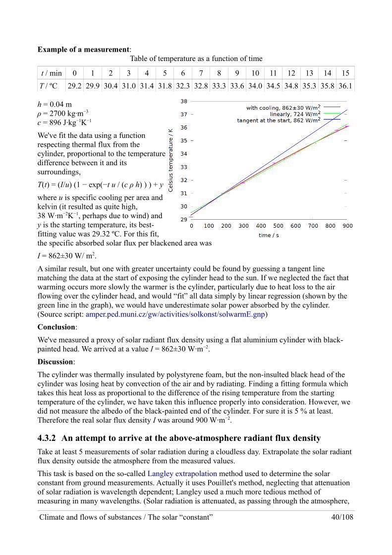
Example of a measurement:Table of temperature as a function of time

t / min 0 1 2 3 4 5 6 7 8 9 10 11 12 13 14 15

T / ºC 29.2 29.9 30.4 31.0 31.4 31.8 32.3 32.8 33.3 33.6 34.0 34.5 34.8 35.3 35.8 36.1

h = 0.04 m ρ = 2700 kg∙m−3

c = 896 J∙kg−1K−1

We've fit the data using a functionrespecting thermal flux from thecylinder, proportional to the temperaturedifference between it and itssurroundings,

T(t) = (I/u) (1 − exp(−t u / (c ρ h) ) ) + y

where u is specific cooling per area andkelvin (it resulted as quite high,38 W∙m−2K−1, perhaps due to wind) and y is the starting temperature, its best-fitting value was 29.32 ºC. For this fit,the specific absorbed solar flux per blackened area was

I = 862±30 W/ m2.

A similar result, but one with greater uncertainty could be found by guessing a tangent line matching the data at the start of exposing the cylinder head to the sun. If we neglected the fact that warming occurs more slowly the warmer is the cylinder, particularly due to heat loss to the air flowing over the cylinder head, and would “fit” all data simply by linear regression (shown by the green line in the graph), we would have underestimate solar power absorbed by the cylinder. (Source script: amper.ped.muni.cz/gw/activities/solkonst/solwarmE.gnp)

Conclusion:

We've measured a proxy of solar radiant flux density using a flat aluminium cylinder with black-painted head. We arrived at a value I = 862±30 W∙m−2.

Discussion:

The cylinder was thermally insulated by polystyrene foam, but the non-insulted black head of the cylinder was losing heat by convection of the air and by radiating. Finding a fitting formula which takes this heat loss as proportional to the difference of the rising temperature from the starting temperature of the cylinder, we have taken this influence properly into consideration. However, we did not measure the albedo of the black-painted end of the cylinder. For sure it is 5 % at least. Therefore the real solar flux density I was around 900 W∙m−2.

4.3.2 An attempt to arrive at the above-atmosphere radiant flux density

Take at least 5 measurements of solar radiation during a cloudless day. Extrapolate the solar radiant flux density outside the atmosphere from the measured values.

This task is based on the so-called Langley extrapolation method used to determine the solar constant from ground measurements. Actually it uses Pouillet's method, neglecting that attenuation of solar radiation is wavelength dependent; Langley used a much more tedious method of measuring in many wavelengths. (Solar radiation is attenuated, as passing through the atmosphere,

Climate and flows of substances / The solar “constant” 40/108

in all wavelengths from UV to IR, but that that attenuation is varying a lot with wavelength especially in IR, see Figure 3 in Glossary.) The intensity of the clear-sky radiation I measured on theEarth's surface depends on the aerosol and water vapour content and distribution in the atmosphere, which can change with time and place, but we shall neglect these changes. The key for us is just the path along which the direct solar radiation must pass. Therefore, in addition to the intensity of radiation, we also have to determine the angular height of the Sun h, from which we calculate the so-called airmass denoted here as m. (Beware, these symbols have a different meaning than in the preceding task.) Then we can plot a graph of I as a function of m (the Langley graph19) and extrapolate I to m = 0, as if outside the atmosphere.

We can get a proxy for solar radiant flux density by:

• a flat aluminium cylinder with a black absorbing head (as in the previous task)

• an instrument intended for this purpose: a pyrheliometer or a Kipp & Zonen CA2 thermopile(see Figure 5.6),

• a semiconductor device – a PV (PhotoVoltaic) panel or an instrument using another semi-conductor sensor. A CEM DT-1307 “solar meter”, let's call it shortly sun-meter, is such an instrument displaying values in W∙m−2. We have to realise that semiconductor sensitivity to radiation is spectrally dependent even as photon flux density is concerned, the more for en-ergy flux.20 Moreover, spectral composition of sunshine is varying during daytime. A reading“in W∙m−2” given by such instrument is but a coarse estimate of solar radiative flux density. Further, similarly as the blackened end of a cylinder, non-adapted sun-meter reacts to irradi-ance from the whole sky; to arrive at direct solar irradiance, we have to subtract a reading obtained when casting a small shadow onto the sensor.

The sample data shown below were obtained using the meter Kipp & Zonen CA2 thermopile. This equipment is calibrated by the manufacturer using a pyrheliometer, which is a rather expensive professional instrument. The CA2 is affordable for the purpose of student measurements at university. It facilitates measuring the intensity of radiation (from sunshine and radiant surfaces) of values up to 2000 W∙m−2. The heart of this sensor is a set of thermocouples, whose black surface absorbs radiation at all relevant wavelengths. The CA2 can be connected to the Meteon data logger, which, if the calibration constant is set,21 displays irradiance in W∙m−2. If you have no data logger, the thermopile can be connected through a voltage amplifier to a voltmeter. The irradiance is obtained by multiplying the output voltage by the calibration constant.

19 As said already, Langley constructed such graphs for radiation measured in shorter spectral ranges, not for all solar radiation together.

20 The instrument gives the same response for blue and infrared photons, disregarding the fact that their energies differby a factor of 2 or more. Further discussion see in part 5.2, On longwave IR radiation.

21 With each CA2 thermopile the producer supplies a protocol with a calibration constant. If long-term measurement stability is required, the thermopile should be recalibrated by the producer regularly.

Climate and flows of substances / The solar “constant” 41/108

Figure 4.6: Measuring direct solar radiation using a CA2 thermopile from Kipp & Zonen.

Figure 4.7: The CEM DT-1307 sun-meter has an affordable price tag (http://goo.gl/aytpF).

The angular height of the Sun

The angular height of the Sun can be either measured using a shadow cast by a ball mounted on a gnomon (an upright stake in the ground) on a horizontal surface or the online application aa.usno.navy.mil/data/docs/AltAz.php. In this application enter the coordinates of your location to get a table of the angular height of the sun (altitude) for the day with a minimum tabular interval of 1 min. For specific measurement time, just look up the corresponding value of h. If measuring the solar angular height h, the obvious equation is tg h = a / b. (The figure below does not show the ball, which should be at the end of the gnomon instead of a sharp tip; only the centre of the shadow of a ball or a disk can be determined accurately.)

Airmass

The so-called airmass m, through which the solar rays travel before reaching the Earth's surface, is merely a number, a relative airmass. It is the ratio of the actual amount of air encountered by the

Climate and flows of substances / The solar “constant” 42/108

direct radiation to that one if the Sun would be shining vertically down to sea level. At sea level, it can roughly be calculated using the formula

m= 1sin h

So, at sea level the airmass m = 1 when the Sun is in zenith (h = 90°). For h = 30°, m = 2; this is often denoted as AM2, when speaking about insolation.

Figure 4.8: Airmasses m = 0, m = 1.0 and m = 2.0.

Expressing airmass with such a simple relationship does not reflect the curvature of the Earth andrefraction of sunlight by the atmosphere. For small angular heights, the m value would be too high, and for h = 0º it would go to infinity, so that we would be unable to see the setting Sun. So, to be able to use this simple relationship, we will measure only when m ≤ 5 (that is, when h ≥ 11,5º)22. Further, we use a “locally relative airmass”, having a local amount of the air contained in the vertical column as a denominator, not an amount corresponding to a sea level site – this is OK for the extrapolation to m = 0.

Table of measured and computed data

time (local solar) h / ° m I / (W∙m-2)

6:30 16.55 3.51 570

7:02 21.77 2.7 663

7:37 27.46 2.17 702

9:02 40.66 1.53 814

9:49 47.05 1.37 837

10:25 51.14 1.28 874Graph

Even if we prefer and use gnuplot now, this old example was processed using a spreadsheet. The vertical axis must be logarithmic (in our example, it is labelled in a deprecated way, see Chapter 9) .The spreadsheet is able to compute the regression line and show its parameters inside the plot. The intercept at m = 0 is the extrapolated solar radiant flux density outside the atmosphere.

22 An alternative application is a programme amper.ped.muni.cz/jenik/astro/lun_illum.php, if the following parametersare entered into command line: c0 zm.

Climate and flows of substances / The solar “constant” 43/108

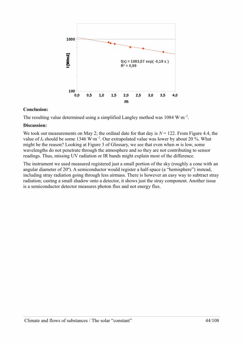
Conclusion:

The resulting value determined using a simplified Langley method was 1084 W∙m−2.

Discussion:

We took out measurements on May 2; the ordinal date for that day is N = 122. From Figure 4.4, the value of I0 should be some 1346 W∙m−2. Our extrapolated value was lower by about 20 %. What might be the reason? Looking at Figure 3 of Glossary, we see that even when m is low, some wavelengths do not penetrate through the atmosphere and so they are not contributing to sensor readings. Thus, missing UV radiation or IR bands might explain most of the difference.

The instrument we used measured registered just a small portion of the sky (roughly a cone with an angular diameter of 20º). A semiconductor would register a half-space (a “hemisphere”) instead, including stray radiation going through less airmass. There is however an easy way to subtract strayradiation; casting a small shadow onto a detector, it shows just the stray component. Another issue is a semiconductor detector measures photon flux and not energy flux.

Climate and flows of substances / The solar “constant” 44/108

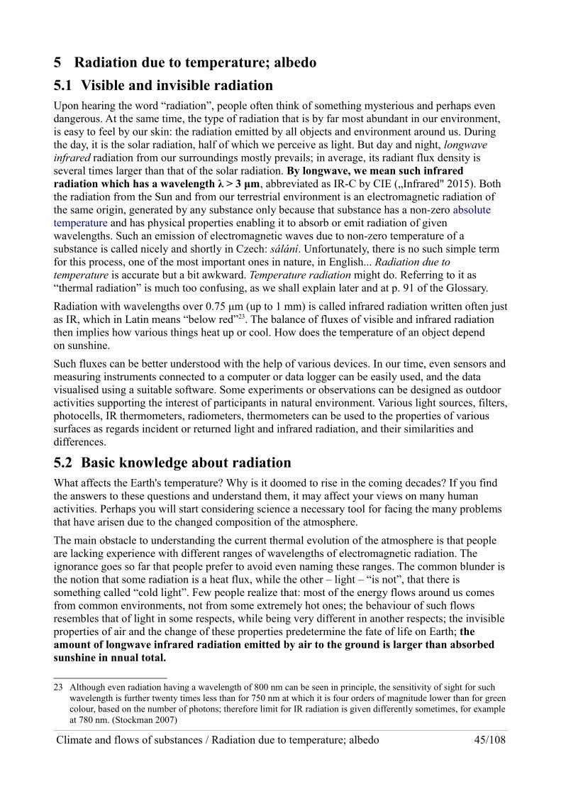
5 Radiation due to temperature; albedo

5.1 Visible and invisible radiationUpon hearing the word “radiation”, people often think of something mysterious and perhaps even dangerous. At the same time, the type of radiation that is by far most abundant in our environment, is easy to feel by our skin: the radiation emitted by all objects and environment around us. During the day, it is the solar radiation, half of which we perceive as light. But day and night, longwave infrared radiation from our surroundings mostly prevails; in average, its radiant flux density is several times larger than that of the solar radiation. By longwave, we mean such infrared radiation which has a wavelength λ > 3 μm, abbreviated as IR-C by CIE („Infrared" 2015). Both the radiation from the Sun and from our terrestrial environment is an electromagnetic radiation of the same origin, generated by any substance only because that substance has a non-zero absolute temperature and has physical properties enabling it to absorb or emit radiation of given wavelengths. Such an emission of electromagnetic waves due to non-zero temperature of a substance is called nicely and shortly in Czech: sálání. Unfortunately, there is no such simple term for this process, one of the most important ones in nature, in English... Radiation due to temperature is accurate but a bit awkward. Temperature radiation might do. Referring to it as “thermal radiation” is much too confusing, as we shall explain later and at p. 91 of the Glossary.

Radiation with wavelengths over 0.75 μm (up to 1 mm) is called infrared radiation written often justas IR, which in Latin means “below red”23. The balance of fluxes of visible and infrared radiation then implies how various things heat up or cool. How does the temperature of an object depend on sunshine.

Such fluxes can be better understood with the help of various devices. In our time, even sensors andmeasuring instruments connected to a computer or data logger can be easily used, and the data visualised using a suitable software. Some experiments or observations can be designed as outdoor activities supporting the interest of participants in natural environment. Various light sources, filters,photocells, IR thermometers, radiometers, thermometers can be used to the properties of various surfaces as regards incident or returned light and infrared radiation, and their similarities and differences.

5.2 Basic knowledge about radiationWhat affects the Earth's temperature? Why is it doomed to rise in the coming decades? If you find the answers to these questions and understand them, it may affect your views on many human activities. Perhaps you will start considering science a necessary tool for facing the many problems that have arisen due to the changed composition of the atmosphere.

The main obstacle to understanding the current thermal evolution of the atmosphere is that people are lacking experience with different ranges of wavelengths of electromagnetic radiation. The ignorance goes so far that people prefer to avoid even naming these ranges. The common blunder is the notion that some radiation is a heat flux, while the other – light – “is not”, that there is something called “cold light”. Few people realize that: most of the energy flows around us comes from common environments, not from some extremely hot ones; the behaviour of such flows resembles that of light in some respects, while being very different in another respects; the invisible properties of air and the change of these properties predetermine the fate of life on Earth; the amount of longwave infrared radiation emitted by air to the ground is larger than absorbed sunshine in nnual total.

23 Although even radiation having a wavelength of 800 nm can be seen in principle, the sensitivity of sight for such wavelength is further twenty times less than for 750 nm at which it is four orders of magnitude lower than for greencolour, based on the number of photons; therefore limit for IR radiation is given differently sometimes, for example at 780 nm. (Stockman 2007)

Climate and flows of substances / Radiation due to temperature; albedo 45/108

Of the manydifferent activities that can be performed in the laboratory or outdoors, we have chosen just a few for you: observations, measurements and experiments.

On (solar) illuminance and irradiance

Do we perceive the amount of light? Not really, what we see is only the luminance ratio in different directions or different consecutive times. Only when the light levels around are very low, such as at the end of evening civil twilight, do we begin to realize the amount of light, as we cease to see the smallest details and even to recognize colours. People are often surprised that solar cells cannot provide enough electricity to power different toys in strong interior lighting. No one notices that even under the overcast winter daytime sky, there may be ten times or a hundred times more light asinside. Our vision adapts to the environment. But PV (PhotoVoltaic) cells or plants are dependent onthe absolute amounts, not on ratios. Witnessing how the illuminance of a luxmeter24 sensor varies from hundredths of lux to a tenth of a megalux in common urban environments during the night andthe day is a useful exercise.

How does this range corresponds to irradiance? Can we use a luxmeter reading as a proxy (or representative) for solar irradiance? A hint can be obtained by common instruments similar to luxmeters, let's call them sun-meters, as already in part 4.3.2.

How do they differ from luxmeters? And from true pyranometers? Luxmeter indicates a good approximation to a variable known as photopic illuminance, because its spectral sensitivity is made very similar to the human vision in daylight. Pyranometers measure the radiant flux density in a spectral range large enough to include almost all incident solar radiation, typically from 300 nm to 2800 nm, using a black-coated thermopile. Sun-meter is akin to luxmeter, recording the flux densityof photons filtered along a “spectral response curve”. It differs from luxmeter in having this response curve “raw”, using the full spectral sensitivity of the silicon sensor. Silicon sensitivity curve is almost flat in the domain of photon flux from 400 nm to 1000 nm. As the photon energy is inversely proportional to the wavelength, the silicon detector is nearly three times less sensitive to the short-wave end of the interval than to the long-wave end when expressed in energy domain. Even though if is possible to filter out the longer wavelengths to achieve flat energy-spectral sensitivity, such filters are usually not applied. The reason for this is that such devices are intended for the assessment of PV plants that respond to photon flux, not to the energy flux equal to solar heat per unit of time. But even pyranometers have their problems (Gueymard a Myers 2009). In contrast, there are PV sun-meters that simply ignore solar infrared radiation, but are well suited for some purposes (Martínez, Andújar, a Enrique 2009).

It may be instructive to compare luxmeter and sun-meter readings. Using them under a clear daytime sky will soon show soon that luxmeter gives a good proxy measurement of solar radiation relevant to photovoltaic cells, the ratio being around 100 lx / (W/m2). This is due to the fact that solar radiation from a clear sky has no significant spectral features that change (see Glossary, Solar spectrum). The ratio is slightly larger for a cloudy sky; the obvious explanation is that water droplets absorb infrared radiation. But for the solar radiation returned back up from the ground the ratio can be quite different, if the surface is coloured, or “coloured”. The term “coloured” in quotation marks refers to an invisible characteristic: infrared reflectance may be very different from visual reflectance. Vegetation is the best example of this, as we shall see later. The ratio of luxmeter readings to sun-meter readings is extremely different from the daytime 100 lx / (W/m2) for outdated “hot” bulbs (named incandescent in English), which emit much more shortwave infrared radiation, and for fluorescent and semiconductor (LED) light sources which do not.

24 Luxmeter is a word common either in Czech or German, unfortunately not in English. It is an instrument for measuring illuminance, and as the unit of illuminance is lux, calling it luxmeter is unequivocal. An accurate long name of it would be, of course, illuminance meter. We avoid to call it by a more general term “light meter”, as such a name suits to any instrument measuring radiation using the spectral sensitivity curve matching human (or more generally, even another animal) vision, including luminance meters or exposure meters.

Climate and flows of substances / Radiation due to temperature; albedo 46/108

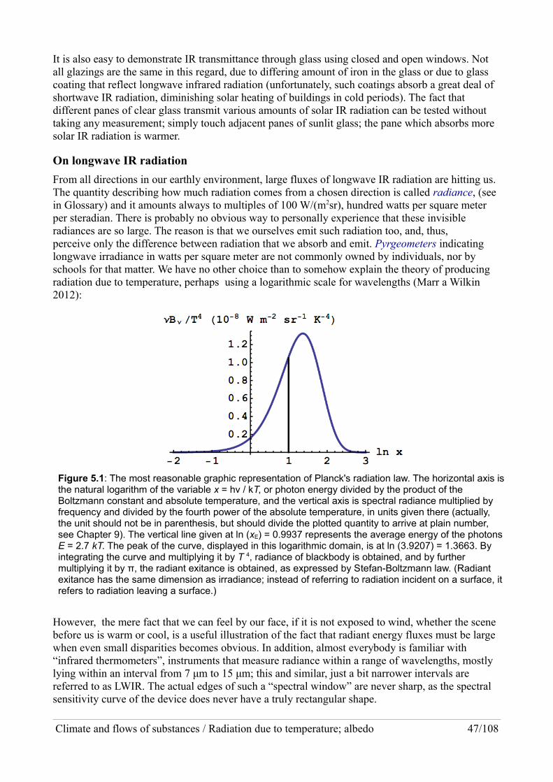
It is also easy to demonstrate IR transmittance through glass using closed and open windows. Not all glazings are the same in this regard, due to differing amount of iron in the glass or due to glass coating that reflect longwave infrared radiation (unfortunately, such coatings absorb a great deal of shortwave IR radiation, diminishing solar heating of buildings in cold periods). The fact that different panes of clear glass transmit various amounts of solar IR radiation can be tested without taking any measurement; simply touch adjacent panes of sunlit glass; the pane which absorbs more solar IR radiation is warmer.

On longwave IR radiation

From all directions in our earthly environment, large fluxes of longwave IR radiation are hitting us. The quantity describing how much radiation comes from a chosen direction is called radiance, (see in Glossary) and it amounts always to multiples of 100 W/(m2sr), hundred watts per square meter per steradian. There is probably no obvious way to personally experience that these invisible radiances are so large. The reason is that we ourselves emit such radiation too, and, thus, perceive only the difference between radiation that we absorb and emit. Pyrgeometers indicating longwave irradiance in watts per square meter are not commonly owned by individuals, nor by schools for that matter. We have no other choice than to somehow explain the theory of producing radiation due to temperature, perhaps using a logarithmic scale for wavelengths (Marr a Wilkin 2012):

Figure 5.1: The most reasonable graphic representation of Planck's radiation law. The horizontal axis isthe natural logarithm of the variable x = hν / kT, or photon energy divided by the product of the Boltzmann constant and absolute temperature, and the vertical axis is spectral radiance multiplied by frequency and divided by the fourth power of the absolute temperature, in units given there (actually, the unit should not be in parenthesis, but should divide the plotted quantity to arrive at plain number, see Chapter 9). The vertical line given at ln (xE) = 0.9937 represents the average energy of the photons E = 2.7 kT. The peak of the curve, displayed in this logarithmic domain, is at ln (3.9207) = 1.3663. By integrating the curve and multiplying it by T 4, radiance of blackbody is obtained, and by further multiplying it by π, the radiant exitance is obtained, as expressed by Stefan-Boltzmann law. (Radiant exitance has the same dimension as irradiance; instead of referring to radiation incident on a surface, it refers to radiation leaving a surface.)

However, the mere fact that we can feel by our face, if it is not exposed to wind, whether the scene before us is warm or cool, is a useful illustration of the fact that radiant energy fluxes must be large when even small disparities becomes obvious. In addition, almost everybody is familiar with “infrared thermometers”, instruments that measure radiance within a range of wavelengths, mostly lying within an interval from 7 μm to 15 μm; this and similar, just a bit narrower intervals are referred to as LWIR. The actual edges of such a “spectral window” are never sharp, as the spectral sensitivity curve of the device does never have a truly rectangular shape.

Climate and flows of substances / Radiation due to temperature; albedo 47/108

5.3 Sample laboratory and outdoor measurements

Non-contact temperature measurement

Question 1: What should we consider when using an infrared thermometer?

Question 2: Do all objects have the same temperature as the surrounding air?

Question 3: Do infrared thermometers give only mediocre results when measuring the temperature of hot water?

We begin our radiation-aimed activities by discussing temperatures, because temperature is the mostfrequently measured quantity in everyday life.

Real thermometer estimates the temperature of its sensor by measuring a temperature-dependent property of the sensor. But even when a sensor hangs freely in the air, aiming at reporting air temperature, sensor's temperature may differ from air temperature despite the reading of the thermometer being almost stable, indicating thermal balance of the sensor with its environment.

This is due to the fact that the sensor responds not just to air temperature, but to radiation fromaround as well. The temperature of sensor should be very close to the air temperature if it has been loosely wrapped in aluminium foil and well shielded from sunshine. Hanging such a wrapped sensor inside a long cylinder made from such a foil would make the sensor's temperature even closer to the air temperature. Without such shielding, solar and other radiation from the surroundingenvironment falling on the sensor greatly affect temperature readings.

A bare sensor, as the common thermometer bulb containing blue or red coloured alcohol, “feels” such radiation similarly like we ourselves do. This is not bad indoors; if there are temperature gradients, like from a cold wall to a warm radiator, we are more interested in how we feel than in what is the air temperature at a given point. The effect of radiation can be amplified using a deep concave mirror made of shiny aluminium foil and by placing a black-coated sensor to its focal point; if you are examining large solid angles, the mirror does not need to have a particularly perfectshape. A cold window or wall in the winter, the cold sky during twilight or at night, the ground that is still warm in the evening, or a hot stove change thermometer readings quite dramatically when the mirror is turned to face them. The temperature of the sensor stabilizes somewhere between the air temperature and the radiant temperature of the surveyed scene.25

Surely, you have seen an outdoor thermometer that gives a temperature that is drastically different from the air temperature, for example, when the thermometer is in full sun in an area protected fromthe wind, it gives a reading that is much warmer than the actual air temperature. The difference of the sensor temperature and the air temperature depends on the absorption of sunshine by the sensor – reflecting mercury bulbs, coloured alcohol bulbs, experimentally black-coated or white-coated sensor bulbs, and bulbs tightly wrapped by alu-foil will give quite different readings. Try it!26

Infrared thermometers do not work this way. They do not indicate the temerapture of the sensor, butthey measure the heat flow (thermal flux) through the sensor and are thus literally “thermo-meters”. This heat flux is generated by longwave infrared radiation from a remote source. The radiation is projected onto the sensor by a special lens that allows less than 2 % of solar radiation pass through it. This is achieved if no wavelengths below 3 μm get through; if the tranmissivity of the lens beginsat 4 μm, less than 1 % sunshine will pass through, and if it begins at 8 μm, the portion of solar

25 By scene, we mean the observed solid angle; it may be some surface and a volume of air and may include objects further in the space outside our atmosphere. It can be studied using its images, or simply by using any integral parameter, like the luminous or radiant flux density coming from this solid angle. Scene: what we see in front of us,or what a chosen observing instrument reacts to in a similar way.

26 On the other side, a novel hi-tech coating has been developed recently, which reflects almost all solar radiation whereas it can radiate through the clear sky to the Universe very well, bringing the coated sunlit surface to a temperature which is below the air temperature (Raman et al. 2014).

Climate and flows of substances / Radiation due to temperature; albedo 48/108

radiation that travels through the lens would be substantially below 0.1 % . The lens is usually madefrom a thick semiconductor; a cheaper options are to use a very thin Fresnel lens made of silicon or a lens from special plastics. Plastic lenses filter solar radiation less thoroughly, since they disperse itrather than absorb it.

All substances except mono- and diatomic gases emit infrared radiation, the radiated electromagnetic output is proportional to the fourth power of the absolute temperature, as stated by the Stefan-Boltzmann law.

Figure 5.2: Radiant exitance of a “blackbody” as a function of its Celsius temperature. According to the Stefan-Boltzmann law, it amounts to 5.67·10-8 W·m-2K-4 T 4, where T is the absolute temperature, i.e., Celsius temperature + 273.15 K.

For temperatures around zero Celsius and radiation confined to the LWIR interval (7 μm to15 μm), temperature dependence is even steeper, being close to the fifth power. Nonetheless, deriving the true temperature of the body from its radiation is not always straightforward. The only variable that can be calculated with certainty is the luminance temperature of a surface in the LWIR band. Let's call this for short the LWIR temperature: the temperature, which a “black body” would have, whosemeasured LWIR radiance27 would be the same.

27 Radiance is a name of a physical quantity (see the Glossary); it is a radiometric analogy of a photometric quantity luminance. It therefore applies to a given solid angle. Devices such as thermal imagers and IR thermometers record a signal proportional to the integral of the product of the spectral radiance of the scene and the spectral sensitivity of the instrument. If this sensitivity curve approaches 1 within the LWIR range and is 0 outside it, we can call this integral a LWIR radiance.

Climate and flows of substances / Radiation due to temperature; albedo 49/108

Figure 5.3: Spectral radiant exitances of a blackbody multiplied by the numeric value of a wavelength expressed in micrometres, for 3 temperatures around the freezing point. The thinner lines are their integrals; at over 200 μm, they achieve values given by the Stefan-Boltzmann law. Source: amper.ped.muni.cz/gw/activities/graphs/sources/plan_sb.gnp

There are two sources of the difficulties in deriving the true temperature. Objects may not be completely opaque to the radiation examined, such as thin plastic films or the Earth's atmosphere without thick clouds. In addition, they may reflect some radiation. Such sources emit radiation proportional to the product of (1-transmittance) (1-reflectance), which is of course within an interval of 0-1 (where 1 = blackbody: no radiation in a given spectral band can pass through it or bounce from it). This product is called emittance. It is often confused with emissivity, but emissivityis a property of optically smooth material28 of sufficient thickness to let no radiation through (its sample has transmittance = 0). Emissivity is a material property of, not the property of any specific object. Real objects may be too thin or have a rough surface. The emittance of rough solid surfaces such as carpets, soil and vegetation is always very close to 1. As shown in Figure 5.2, at 17 ºC they emit an entire 400 W/m2. Shiny steel, aluminium and copper surfaces have an emittance value close to zero, but if corroded, their emittance can be closer to 1 then to 0.

LWIR emittance and transmittance can be measured using two objects with differing temperatures, when the radiation from one of them is reflected by the second one or passes through it. A detailed text describing this in Czech can be found at pages 52-58 of (Hollan 2009a).

But even without a thermometer, we can observe reflection or transmission of longwave infrared radiation, or generally, radiant cooling or heating, using the most sensitive parts of our skin, such as that on our hands or face. Turning your face to the ground and then upwards to the clear evening sky devoid of sunshine, you can feel that the sky (or the air above you) radiates to you appreciably less than the ground. However, on a summer evening, radiation from the sky is still much stronger than that from an open freezer with a temperature of some 255 K. At the same time, even such a

28 Optically smooth, taken strictly, is a surface whose roughness is less than an eighth of the wavelength of the radiation. If the surface looks pretty shiny, mirroring light with good contrast, it is, for sure, perfectly smooth in the range of LWIR wavelengths, as these are twenty times longer.

Climate and flows of substances / Radiation due to temperature; albedo 50/108

very cold object emits good two hundred watts per square meter, see Figure 5.2. Think about how cool the heavens would be without the greenhouse effect; the night universe above us has a radiant temperature of only 4 K. It emits almost no radiation to us; in order to emit a mere 1 W/m2, temperature of almost 65 K is needed.

Figure 5.4. shows examples of measured radiation of the air down to the ground; you can see that inour mid-latitude regions, it changes mostly between 220 W/m2 and 350 W/m2 during the year, outside high mountain sites.

Figure 5.4: Temperature radiation of the sky to the ground at two Swiss stations: Payerne (b., 490 m above sea level) and Jungfraujoch (d., 3580 m). The vertical axis gives irradiance in watts per square metre, the horizontal one gives the year. The data are for each 10 min; dark blue holds just for times of cloudless sky. It is evident, that especially at the top of Jungfraujoch, clouds contribute a lot to the radiation toward the ground. This is due to the fact, that the air contains just a very little amount of watervapour above this high altitude. The light blue curve shows mean values for cloudless conditions. The seasonal cycle is prominent. The Payern station is well comparable with lowlands regions of Czechia and other mid-latitude sites, in respect of downwelling longwave infrared radiation. Source: Figure 2 in Wacker et al. (2011). That paper shows further, that at this lower-lying station, the downwelling radiationfrom the cloudless air increased by some 5 W/m2 over the plotted period, probably due to a combined effect of an increase of temperature and of water vapour content.

Pointing a non-contact thermometer upward at the zenith, we can estimate the water content in the air (Mims, 2011), because we can detect the IR radiation of water vapour molecules. Some infraredthermometers can not be employed for this purpose, as their zenith reading under clear sky gets below the lower limit of the device range; the LWIR interval is just that one, where the cloudless airradiates the least. But even such IR thermometers can be employed to estimate the altitude of the base of cumulus clouds. This is because the existence of a temperature gradient of the convective air beneath cumulus clouds, amounting simply to 0.01 K/m, meaning 1 K for every 100 m. And because any non-transparent cloud behaves like a blackbody in LWIR, by measuring sky “luminance” temperature, we get a good proxy for the true temperature of the cloud base.

Finally, if the IR thermometer detects radiation from a cone that is slim enough, it can be surely used to demonstrate the basic greenhouse effect of, i.e., the temperature radiation of even the cloudless air. Even if the thermometer reports “out of range” reading in zenith, in angular heights which are low enough, it would start to indicate some LWIR temperature, the higher the closer to horizon. This is because a longer column of air is being observed near horizon. Very close to horizontal direction, the air is non-transparent even in the LWIR interval when humid enough (in maritime mid latitudes, this is always the case in summer), so the thermometer indicates a temperature not very different from the ambient air temperature. Of course, an imaging device, a LWIR camera, is a lot better for such visualisation, as radiation from the land and sky is clearly divided.

Climate and flows of substances / Radiation due to temperature; albedo 51/108

Figure 5.5: Measuring the LWIR temperature of the sky near zenith using an IR thermometer

Measuring illuminance and albedo

Question 4: How dark is a given surface? How bright?

Any area may appear dark when it is less illuminated than its surroundings. Or – even if it is quite black – it may seem bright, if it reflects a source of light, such as the Sun, into our eyes. Various surfaces can be described as being “white”. However when placed side by side, they may differ greatly. In science, whiteness is called albedo (from the Latin albus, white). It is a mere number lying within an interval between 0 and 1. It indicates the proportion of incident light that goes back from the surface to the incident half-space, as a response to the incident radiation.29 Whiteness values are important for interior lighting. In a broader sense, albedo may concern the entire spectrum of solar radiation, including its invisible UV and IR components. To calculate such broadband albedo, energy-based quantities and not human-vision-based ones are used. Solar albedo is the variable, from which the shortwave radiant heat flux absorbed by the Earth can be calculated.

Visual albedo of a flat terraine can be easily measured by a luxmeter. Hold the sensor, pointed downward, in your outstretched arm about 2 dm above the ground. Then take a second reading withthe sensor turned towards the sky. The ratio of the two resultant values is the photopic visual albedo,as luxmeters are designed to imitate the spectral sensitivity of the human daylight vision.30

Measurement taken with the sensor turned towards the ground represents total light that goes upwards, if the sensor is “Lambertian” or “cosine” type – i.e., when the signal it captures corresponds to the true illuminance of the plane of sensor's entrance31. Illuminance is the integral of

29 Goes back... by reflection, as if from a mirror, by diffusion (i.e., to directions differing from the angle of incidence) and, eventually, by luminescence. If the incident radiation is dominated by the UV component and the irradiated material exhibits photoluminescence, the surface may return more than the incident amount of light... and visual albedo may be over 1: for the given spectrum of the incident radiation. So, taken thoroughly, albedo is not a property of the body itself, but of the body and the spectral composition of the incident radiation and also its angle of incidence. In case of direct sunlight, the amount of UV is never large enough to get visual albedo over 1. Even so, the amount of returned light is commonly enhanced by luminescent chemicals within white paper or in washing powders, to achieve an impression of wonderfully white stuff.

30 Let's remark that spectral sensitivity of fully dark-adapted human night vision is shifted to shorter wavelengths and is called scotopic; there exists a complete of alternative visual photometry based on this spectral sensitivity. Unfortunately, it is tied with photopic photometry by saying the sensitivity at 555 nm is the same. This implies that for daylight (and moonlight) spectral composition of light, scotopic values of all photometric quantities are about thrice the photopic ones. An alternative concept has been proposed to express photopic-like sensations (Hollan 2009b).

31 The sensitivity of such a sensor is independent on the angle of incidence of radiation. Of course, the total radiation incident on the sensor is proportional to the cosine of the angle of incidence. Similarly, a cosine radiator is a such that its radiance is the same in all directions (or in the case of light, whose luminance does not depend on how the light-emitting surface is angled towards you). A Lambertian diffuser is a surface whose luminance is independent not only on the direction from which you observe it, but also on the direction from which it is illuminated, provided

Climate and flows of substances / Radiation due to temperature; albedo 52/108

the luminous flux density multiplied by the cosine of the angle of incidence, taken over the solid angle of 2π sr. Luxmeters always try to imitate this feature. It is not difficult to verify how well succeed at this. Point the sensor at a dominant light source (e.g., the Sun) and record the luxmeter's reading. With the Sun high in the sky, it should be a tenth of a megalux. Take another measurement when you cast a small shadow so, that just the sensing area is covered by it. The difference between the two readings is the direct solar illuminance. Then attach the sensor to a long thin rod so that the plane of the input aperture (pupil) of the sensor is parallel to the rod. Point the rod almost at the Sun, but so that its shadow cast on a plane perpendicular to the Sun will be ten times or five times shorter than the length of the rod. The plane showing the shadow can be a ruler or cardboard on which a fifth or a tenth of the rod's length is indicated. Again, take two measurements, the latter of which should be taken with the same small shadow cast onto the sensor. If the detector is Lambertian, then the direct solar illuminance, as measured by it, is five or ten times smaller than in the case of the sensor facing the Sun.

Figure 5.6: Verifying Lambertian (cosine) sensitivity of a luxmeter sensor. Instead of the shadow of a rod, the shadows of two sticks inserted into the ruler are used, as the centres of their shadows are unequivocal.

But even with a Lambertian detector it may not be easy to measure all the light returned to the half-space by the selected material, unless its surface is so large that it takes up the vast majority of the solid angle of 2 π sr to which the sensor is pointing. The solid angle occupied by the material under investigation (by the sample) can be easily increased putting the sensor closer to material. On the other hand, the space angle occupied by the sensor's shadow grows as well. The shadow plays a lesser role when most of the light comes at an angle, which is common in practice. But even if the sun shines almost perpendicularly onto the probed surface, the shadow cast by the sensor might should not matter much. Consider a case when the distance between the sensor and the examined surface is two times greater than the diameter of the sensor (and hence of its shadow). Then the

its illuminance remains the same. Common surfaces behave only approximately in this way, since they usually sendan excess of radiation roughly like a mirror, at an angle equal to the angle of incidence. The adjective lambertian is named after 18th century physicist J. H. Lambert, who dealt with optics as well.

Climate and flows of substances / Radiation due to temperature; albedo 53/108

shade takes only 0.2 sr, which is just over 6 % of the value you get by integrating the cosine of the angle of incidence over the half-space (2 π sr), since this integral is π sr.

And what effect does limiting the radius of the investigated surface have? If the radius is five times the distance of the sensor, then the remaining ring, which is no longer filled by the sample from the view of the sensor, has a thickness of only 0.2 rad, which corresponds to a loss of about 5 % of the signal from the sample. This is not a big problem if the sample's surroundings do not differ much from from the sample itself, i.e. if their luminances are similar. Even if luminance differs greatly, the influence of the environment can be estimated, together with the effect of the shadow cast by the sensor. Figure 5.7 should provide help sufficiently for such calculations.

Albedo of a surface is somewhat dependent on the prevailing direction of the incident light so that itslightly changes with the angular height of the sun in the clear sky. Most surfaces reflect more light when illuminated almost tangentially. Compare e.g. river, asphalt, grass...

Solar albedo in a bit broader spectral window

Question 5: How different is solar albedo compared to visual albedo?

Sun warms the Earth's surface during the day. Most of the incident Sun's radiant heat flux is absorbed by oceans and continents. The rest is returned back up through the air. Full solar albedo, orthe ratio “not absorbed radiant energy / incident radiant energy” is a parameter describing the examined surface. For the Earth as a whole, solar albedo amounts to one third, which is several times higher than the albedo of the oceans and the continents. This is due to clouds, which, viewed from above, are always quite white.

So how dark is the very surface of the Earth, as regards full incident solar spectrum? It can be quantified using instruments similar to luxmeters, if they are capable of capturing the infrared part of the solar radiation spectrum, i.e., waves that are longer than those corresponding to red light. In

Climate and flows of substances / Radiation due to temperature; albedo 54/108

Figure 5.7: The effective solid angle from which a Lambertian detector gets its signal. It is plotted as a function of the angular radius of the cone from which the radiation is recorded. Thefirst ten degrees contribute very little to the total signal, the same holds for the last ten degrees.(amper.ped.muni.cz/gw/activities/graphs/sources/illuminanceP.gnp)

this way, it can be found that the properties of many surfaces in the visual range and in a broader range of wavelengths are not that different.

For vegetation, however, these properties differ a lot... Vegetation absorbs majority of visible radiation (light), but if we take the whole sum of solar radiation that lands on it, then the absorbed fraction is several times smaller. Thanks to that, vegetation is not heated so much during the day, even if it absorbs most of light to conduct photosynthesis. (For example, from one set of our measurements of a surface covered with grasses and dicots, the ratio “solar_up / solar_down” was 1/2.5, while the ratio “visual_up / visual_down” was 1/14.) The property of vegetation, that it rejects much more infrared than red, is used to monitor its extent and health from satellites or planes, using an index called NDVI.

For observation made under varying conditions, where inhomogeneous cloud cover is moving across the sky, a set-up using two instruments simultaneously can be chosen. In this way, downwardand upward radiant fluxes can be measured at once. You can use two luxmeters, but using just one luxmeter and one sun-meter can do.

Figure 5.8: Measurement of solar albedo of forbs and grasses using a sun-meter in non-variable conditions (cloudless sky). The sensor is kept 3 dm above the ground. The image on the left shows the radiation returned upwards being recorded; the one on the right one depicts the recording of incident solar radiation. The same procedure is used for measuring visual albedo with a luxmeter. Attaching the sensor to a 1 m lath is better than holding the sensor in your hand, as you, the observer will be farther from sensor, which will limit the the influence of your shadow. Of course, you should stand so that your shadow goes away from the sensor.

Experiments with cooling and heating

Question 6: Many researchers recommend painting roofs white to slow down global warming. Why?

To answer this you need to understand the balance of radiation entering the Earth's atmosphere and the radiation going from the atmosphere into space. During the day, a white surface returns most of the solar radiation back up, so it is warmed by the Sun as little as possible. But it has another important property as well, namely that it efficiently emits longwave infrared radiation, cooling itself this way. Thanks to that, a sunlit white surface is much cooler than an aluminium or any metallic non-painted surface. Shiny aluminium may well reflect as much radiation as a very white surface, but starting at the same temperature, aluminium emits much less radiation than white paint:it has a very low emittance. The temperature of glossy aluminium, if it is thermally insulated from below, stops rising only when it is much warmer than the air that is removing heat from it. Non-metallic surfaces, in contrast, send heat off by radiating into the sky. This radiation heats up the air kilometres above them, and a small part of such radiation proceeds through cloudless air straight

Climate and flows of substances / Radiation due to temperature; albedo 55/108

into space. White-painted roofs reduce summer overheating at places with a hot, sunny climate; they can greatly improve comfort in the city. In addition, they can reduce the present imbalance of energy flows absorbed and emitted by the Earth, even if only slightly. Similarly, bright, perhaps even white pavements and walls – such as those in Mediterranean towns made of white limestone oreven whiter crystalline limestone, i.e., marble. Marble helps also due to its high thermal conductivity: during the day heat goes deep into the pavement instead of warming the air; the temperature difference between day and night is reduced this way.

On the other hand, if something should be kept warm at night, radiant cooling can be greatly suppressed utilizing an aluminium coating. “Space blankets”, which consist of thin aluminized plastic foil, are commonly used for rescuing injured people. Interestingly, even if the foil is gold-tinted over the aluminized side, it suppresses temperature radiation almost as well as pure aluminium coating with no varnish (this is due to the varnish layer being extremely thin). The gold-painted surface is of course more heated by sunshine, so such such space blankets with their golden side up are more convenient for protecting people from the cold during the day.

Figure 5.9: White paper and aluminium foil – how they warm up and cool down. The graph shows a very simple sample measurement. The temperature sensors were under sheets of either material. The right y-axis shows a rough indication of illuminance (real values were probably under 110 klx, since higher values may occur only when white clouds redirect sunlight from shaded places to sunlit ones). An improved arrangement would be to use thicker aluminium sheets with variously treated surfaces. One sheet with a paper on it, the other with a fresh, shiny aluminium foil cover, both glued tightly to the sheet. The sensors should be glued to the bottom surface of thick sheets, which conduct heat well.

Observing spectra

The above activities relate to the integral characteristics of radiation, be it shortwave (< 3 μm) radiation or longwave infrared. Sometimes a detailed distribution of radiation by wavelength may be important. This is generally called spectrum, a Latin word for an apparition or a ghost – indeed, creating a palette of vivid colours from “boring” white light using a clear, colourless equipment is quite impressive “magic”. With a bit of practice spectra can be easily viewed and even photographed using non-mirror reflections from CD and DVD discs. (It is even better is to use the same grooved discs, but uncoated, looking through them; such uncoated DVDs are sometimes at thebottom of their stack as sold in shops). For more see thesis Nedvěd (2007, in Czech).

Climate and flows of substances / Radiation due to temperature; albedo 56/108

Figure 5.10: By taking a picture of direct sunlight, the spectral calibration of a camera with a fisheye lens can be achieved, because in the photo spectral lines are visible (Hollan 2008).

Climate and flows of substances / Radiation due to temperature; albedo 57/108

Figure 5.11: Raw spectral records for three artificial sources weencounter daily – a fluorescent lamp, a white LED and anoutdated hot wire inside a bulb (called incandescent). The lightemitted by all these sources is perceived as white, but itsspectral composition is different. The vertical axis of the chartsshould correspond to the spectral radiant exitance. The spectrawere measured with a school SpectroVis Plusspectrophotometer with SpectroVis Optical Fiber made byVernier. It can be connected directly to a computer via a USBconnector. The price of this spectrophotometer is about 800 €,You can not expect it to provide precision similar to professionalequipment whose prices are much higher. Nevertheless, it canbe used for school and laboratory tasks designed to investigatelight and the optical properties of solutions.

From the recorded spectrum of the incandescent source, a hottungsten wire, it can be estimated that it contains artefacts,waves that are not real. The real shape of the spectrum ofincandescent tungsten filament has to be close to the spectrumof a blackbody of the same temperature, as emittance of thefilament does not vary wildly with wavelength. Radiation shouldmonotonically increase to the right edge of the chart and further.Simplified theoretical spectra of lamp filaments (assumingemittance of 0.4, really it is half that amount for wavelengthsabove 2 μm) are shown below. It is clear from them that light(wavelengths roughly from 0.4 μm to 0.75 μm) account for just asmall part of the radiant power.

(Source script: amper.ped.muni.cz/gw/activities/graphs/sources/bulbs_colPh.gnp)

Climate and flows of substances / Radiation due to temperature; albedo 58/108

5.4 Conclusions and discussionIn this chapter, we offered some hints to for exploring very common processes and variables, yet wedid not discuss in detail the metrological jungle of radiometry and photometry. We believe that teachers and students will find other approaches to such activities aimed at learning radiative energyfluxes hands-on. And that when conducting similar measurements, the terminology used in these fields becomes manageable, perhaps even interesting for them, step by step. At the beginning though, referring to chapter “Glossary” may be of help to them.

Commented pictures of activities that we have described and the source files of original charts in this publication are available at http://amper.ped.muni.cz/gw/activities.

5.5 Remark: the Snowball Earth ideaEarth's albedo is of great importance for the Earth's overall energy balance and thus for the global climate. According to satellite measurements, the average solar albedo of the Earth is 29 % ( ± 2 %). However, the Earth has undergone at least two periods of almost global continental glaciation,when ice sheets reached up to or near the equatorial region, as documented by geological evidence: in ocean areas that were near the equator during these glaciations, boulders at their floor transportedthere by icebergs have been found. These icebergs calved off from ice flows that extended into the sea. When the icebergs thawed, they released dropstones that fell to the ocean floor. There is even an idea known as the Snowball Earth (Kirschvink 1992), which may seem absurd at first. If whole Earth was covered by ice and snow, it must have reflected so much sunshine that it could never melt, could it? However, volcanoes were active even during glaciation and they produced carbon dioxide which accumulated in the cool and dry atmosphere. The resulting greenhouse effect could be so strong that the ice had melted and the Earth quickly moved into the hot state in which no ice at all existed. Snowball Earth model is helpful for understanding the significance of carbon dioxide for global climate. Videos on those glaciations are by BBC Horizon, www.bbc.co.uk/nature/ancient_earth/Snowball_Earth and National Geographic, channel.nationalgeographic.com/channel/videos/snow-ball-earth/. However, it seems sure that equatorial ocean was not perennially covered by ice even in maxima of glaciation during Cryogenian period (and, therefore, the hydrological cycle dependent on evaporation was never halted), see, e.g., papers on possible minimum carbon dioxide levels (Feulner a Kienert 2014) and on biological processes (Lenton et al. 2014).

Climate and flows of substances / Radiation due to temperature; albedo 59/108

6 Biochar6.1 Biomass as an energy sourceThe rising population of the world and the growing sum of GDPs (=GWP, gross world product) have|created a growing demand for raw materials and energy resources. Biomass is the traditional energy source that was used by people to heat and cook until recently. Before the introduction of modern agricultural machines powered by oil products, cattle was used to pull various cultivating tools and carts or carry loads; farmers had to grow enough feed for these working animals. Inagriculture, biomass used to be the dominant source of energy well into the 20th century even in the most developed countries. In the 1940s in Europe, besides draft animals and fossil-fuel-powered equipment, machines with engine running on wood gas had been used. Wood gas is produced through the pyrolysis of biomass; when heated to temperatures around 450 ºC, biomass is convertedinto char and a fluid component known as wood gas. Wood gas was eventually completely displaced by oil in transport.

Today, the about 11 % of the world's total “consumption” of primary energy comes from biomass. The dominant energy source are fossil fuels, which provide more than 80 % of energy flux created or actively captured for the needs of civilization. Biomass is mainly used to produce heat for cooking (in the developing world) and for heating buildings. A small fraction is being used to perform mechanical work by thermal engines which are coupled to electricity generators convertingmechanical work to electric work. The best current use of biomass happens when also the heat inevitably flowing out from thermal engines is used reasonably. Or vice versa, if not all the heat produced by burning biomass is used for the ordinary heating of buildings, but the initial high temperatures are used for running such a system of thermal engine – electric generator. Such an alternative to ordinary heating is called co-generation: electricity is produced besides the further utilised heat.

Biomass can be used to produce wood charcoal, which is a widely used energy source for households in developing countries. It is used mainly in large towns, as compared with firewood it is easier to transport and produces less smoke when burning. During the traditional production of wood charcoal in clamps (structured pile of wood covered with soil), wood gas, a major polutant, escapes through cracks in the soil or a chimney. The combustible components of emitted wood gas, namely CO, CH4 and H2, are not utilised in such wasteful production. Wood gas contains some 23 % CO, 2 % CH4, 14 % H2, 51 % N2 and 10 % CO2, relative to its volume, i.e. to number of its molecules. The ratio of individual components varies for different pyrolysis temperatures and typesof biomass. The process of making wood charcoal this way (see more in German wikipedia item Kohlenmeiler) takes several days, depending on the size of pile. Traditional Meiler can have a yield as low as 10 %, which means that from 10 kg of wood, we obtain 1 kg of charcoal. More sophisticated devices can attain a yield of 50 % and have lower harmful emissions.

When burning wood in an open fire or in a simple wood gas stove, substantial portion of wood gas is not burnt and escapes into the atmosphere. This unwanted emission contains 80–370 g of carbon monoxide and 14–25 g of methane per kilogram of wood burned (Larson a Koenig 1993). If fumes from stoves are drained away through a chimney, from time to time the non-oxidized wood gas along with the soot covering the inside of the chimney will flare up. Today, there are modern household heating systems on the market, i.e., fireplaces and stoves with better secondary combustion, which allows the complete combustion of wood gas. These devices reduce fuel consumption for heating along with air pollution in the process. Modern stoves for heating and cooking are designed so that they burn fuel as efficiently as possible.

During the Holocene, the amount of biomass on Earth was nearly constant. Carbon fixed by photosynthesis merged again with oxygen by respiration of plants and animals and due to decomposition of biomass by fungi and microorganisms, or it was oxidized abruptly during fires.

Climate and flows of substances / Biochar 60/108

The flow of carbon through biosphere was enhanced by farming practices, particularly soil cultivation and fertilization, but the total carbon content of soils actually declined, as did forest biomass due to slash-and-burn forest clearing. In comparison, the ongoing energetic use of aboveground biomass stocks implies no steady reduction of the carbon content of existing biomass; whether biomass is oxidized through spontaneous composting or combustion is not that important. Leaving the landscape to its fate, would cause the mass of carbon resting on the surface of the soil, where it would wait for a couple of years to oxidise naturally, to increase a bit, but this would not result in the creation of a large, permanent carbon pool. The use of biomass by humankind is simplya shortcut in the rapid circulation of carbon between the biosphere and atmosphere, which is processthat would occur anyway.

The extraction and oxidation of fossil fuels, in contrast, mobilizes carbon that would otherwise remain in sediments hundreds of thousands of years (in the case of peat ) to hundreds of millions of years (all other fossil fuels). Burning biomass is therefore neutral in terms of the carbon cycle, whilethe extensive burning of coal and other fossil fuels has compromised the dynamic balance of the carbon cycle and caused accumulation of CO2 in the atmosphere and oceans. Nine tenths of current anthropogenic emissions of CO2 are caused by burning fossil fuels; a tenth at most is due to deforestation and some 1/20 is due to cement production (Le Quéré et al. 2013, see also http://www.globalcarbonproject.org/, for presentations featuring many graphs).

6.2 Production of biochar and its benefitsFigure 6.1 shows the traditional practice of using biomass in developing countries, at left. Meals areoften prepared on an open fire with three stones serving to support a pot. This cooking method is wasteful because more than 80 % of the energy is not used. The consumption of firewood is high, and many pollutants are released into the air. They include soot which, like greenhouse gases, emits infrared radiation down to the surface when airborne and, in addition, strongly absorbs solar radiation, thus significantly contributing to global warming (Ramanathan 2007). Poor farmers are forced to buy mineral fertilizers to help them obtain at least some crops from the depleted soil. On the right, the figure shows the traditional fireplace replaced by a simple wood-gas stove, which usually has a thermal efficiency rate of about 50 %. Cooking requires less fuel, plus, instead of wood, residues from agricultural production that do not burn well in an open fire (seeds, shells, sugar cane stem pulp) can be used. When wood gas is burned for cooking, less toxins andgreenhouse gases are emitted. Once the flame is extinguished, it means that the biomass has thoroughly undergone pyrolysis. The resulting char is then crushed and added to the soil, thereby improving its physical properties. Farmers can increase crop yields utilising a minimum quantity of fertilizers, those of organic origin (compost, manure, nitrogen-fixing plants) may do. The farmer saves a large amount of money avoiding the need to buy mineral fertilizers. Carbon remains in the soil for centuries. Char from biomass that is made to be added to the soil, is called biochar in the scientific literature.

Climate and flows of substances / Biochar 61/108

Climate and flows of substances / Biochar 62/108

This technology provides a “win-win-win” solution to global problems (like killing three birds with one stone): (1.) It allows efficient use of fuel wood (or waste biomass) for cooking; (2.) It rectifies the quality of the soil depleted by intensive agriculture; and (3.) It stores carbon acquired through photosynthesis from the atmospheric greenhouse gas CO2 and has the potential to significantly reduce the rate of anthropogenic climate change.

In addition, biochar, thanks to its ability to effectively hold fertilizers in the soil, can significantly reduce fertilizer use and thus prevent eutrophication, which is, beside global warming, another serious environmental problem worldwide. The production of mineral fertilizers is very energy-intensive process dependent on fossil fuels. If biochar was added to the world's agricultural soils, it could much reduce the consumption of the fossil fuels associated with the use of mineral fertilizers (from the mining of phosphate rock, through the production and transport of fertilizers from manufacturers to farmers, to applying the fertilizer to the soil) and thus significantly reduce anthropogenic emissions of greenhouse gases.

For more on biochar in Czech with lots of English references see amper.ped.muni.cz/gw/uhel/.

6.3 How do wood-gas stoves work?There was a lack of liquid vehicle fuels during World War 2, and therefore, many car in Europe used wood gas instead. Each wood-gas car was fitted with an Imbert generator (De Decker 2010), into which logs were loaded from above and from which wood gas was discharged through the bottom into a combustion engine. Gas flow through the generator was directed downwards (downdraft). All the biomass in the generator was burnt to ash after pre-drying and pyrolysis.

It was not until the 1980s that the TLUD pyrolysis principle, which is usable for cooking, was discovered. TLUD means Top-Lit UpDraft. A diagram of a TLUD stove made of three cans is shown in the figure below32. The procedure for operating the stove is as follows: The internal space is filled with dry biomass (sticks, shells, kernels, etc.). The top layer is best made of materials such as shavings that easily ignite, and thus create a glowing layer to start pyrolysis. The pyrolysis zone then shifts downwards until the biomass load is charred throughout. The heating of the biomass produces wood gas. A small portion of wood gas is burned in the pyrolysis zone (primary combustion) at temperatures around 800 ºC and limited oxygen availability. The heat released keepspyrolysis continuing (pyrolysis itself is an endothermic process, i.e. it consumes heat). Most of the wood gas goes up, where it is mixed with preheated air transported there by the stack effect, which arises in the hot hollow wall of the stove. There, at the top of the stove, secondary combustion takesplace, which can be utilized for heating the cooking pot. Upward draft of the air through the stove can be enhanced by adding a simple chimney. Once the flame goes out, the resulting char should be

32 Animation of the pyrolysis process of a TLUD stove can be found online: www.youtube.com/watch?v=m2Cjt7AiZJY.

Climate and flows of substances / Biochar 63/108

Figure 6.1:Comparison of traditional biomass use in developing countries (left) with the use of biochar, which is produced in simple wood-gas stoves (Whitman a Lehmann 2009).

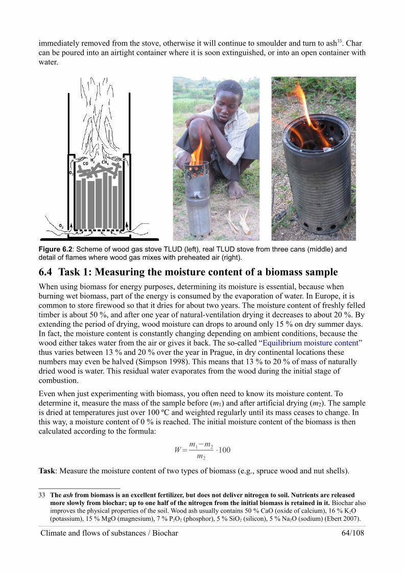
immediately removed from the stove, otherwise it will continue to smoulder and turn to ash33. Char can be poured into an airtight container where it is soon extinguished, or into an open container withwater.

Figure 6.2: Scheme of wood gas stove TLUD (left), real TLUD stove from three cans (middle) and detail of flames where wood gas mixes with preheated air (right).

6.4 Task 1: Measuring the moisture content of a biomass sampleWhen using biomass for energy purposes, determining its moisture is essential, because when burning wet biomass, part of the energy is consumed by the evaporation of water. In Europe, it is common to store firewood so that it dries for about two years. The moisture content of freshly felledtimber is about 50 %, and after one year of natural-ventilation drying it decreases to about 20 %. Byextending the period of drying, wood moisture can drops to around only 15 % on dry summer days. In fact, the moisture content is constantly changing depending on ambient conditions, because the wood either takes water from the air or gives it back. The so-called “Equilibrium moisture content” thus varies between 13 % and 20 % over the year in Prague, in dry continental locations these numbers may even be halved (Simpson 1998). This means that 13 % to 20 % of mass of naturally dried wood is water. This residual water evaporates from the wood during the initial stage of combustion.

Even when just experimenting with biomass, you often need to know its moisture content. To determine it, measure the mass of the sample before (m1) and after artificial drying (m2). The sampleis dried at temperatures just over 100 ºC and weighted regularly until its mass ceases to change. In this way, a moisture content of 0 % is reached. The initial moisture content of the biomass is then calculated according to the formula:

Task: Measure the moisture content of two types of biomass (e.g., spruce wood and nut shells).

33 The ash from biomass is an excellent fertilizer, but does not deliver nitrogen to soil. Nutrients are released more slowly from biochar; up to one half of the nitrogen from the initial biomass is retained in it. Biochar alsoimproves the physical properties of the soil. Wood ash usually contains 50 % CaO (oxide of calcium), 16 % K2O (potassium), 15 % MgO (magnesium), 7 % P2O2 (phosphor), 5 % SiO2 (silicon), 5 % Na2O (sodium) (Ebert 2007).

Climate and flows of substances / Biochar 64/108

W=m1−m2

m2

⋅100

Sample A B

Description

m1

m2

W

Conclusion:

6.5 Task 2: Measuring the yield of char from a wood gas stoveAccesories:

• Wood-gas stove (for an overview see zenstoves.net/Wood.htm,for a self-made stove like that from three cans, goo.gl/gDr3s)

• An electronic scale

• A pot (for pouring and weighing char)

Tasks:

1. Get a sample of dry biomass for the experiment (about 300 g). Find (in tables or on the In-ternet) the properties of the selected types of biomass (heating value, composition) and measure the bulk density of the stove filling.

2. Measure the mass of the biomass before the experiment and the mass of the resulting char. (After the flame extinguish, it is necessary to pour immediately the embers into the pot and weigh them.)

3. Estimate the carbon content of the biomass and of the produced char. What per cent of bio-mass carbon has not been released into the air?

Safety rules:

Start the pyrolysis process by pouring a bit oil over the surface of the biomass fill of wood-gas stoveand setting it on fire. The biomass must be thoroughly dry, otherwise the flame may go out prematurely. Normally, pyrolysis takes place in the stove with no smoke and wood gas burns efficiently. If the flame goes out prematurely (if biomass is wet or the wind blows out the flame) thehot biomass will emit dense smoke. The situation can be solved by reigniting the smoke by a piece of burning paper, or even by dropping some oil again to the surface of the charred biomass and setting the fire anew. This experiment can be performed outside or in a laboratory. If performing theexperiment indoors, you must concuct it under a hood for fume extraction. When working with an open fire, it is necessary to observe fire regulations. The surface of the stove is heated to very high temperatures, so do not touch it with your bare hands. The embers are best extinguished by pouring them into a pot and closing it with an airtight lid.

Table of measured and computed values:

Description of biomass properties(according to tables)

Moisture content W (see Task 1) / %

Climate and flows of substances / Biochar 65/108

Mass of biomass sample / g

Mass of char / g

Yield / % (= 100 * “biomass” / “char”)

Relative amount of carbon in biomass / %

Conclusion:

Remark:

In the above experiment, a considerable portion of the material on the surface of particles of biomass react with the primary air, it oxidizes. Thus, this whole process is better called gasification, which differs from true pyrolysis, a process that does not require oxygen. The yield of char from biomass using true pyrolysis is higher; actual numbers depend on the pyrolisis temperature and the kind of biomass used. This dependence is illustrated well in the following graph.

Figure 6.3: The graph shows the percentage of the dry weight of the biomass remaining after pyrolysis in the form of char. The yield is higher at lower temperatures and also depends on the type of biomass. Taken from Demirbaş (2001).

Suggestions for further experiments with biochar:

• Measure the efficiency of wood-gas stove and compare with other types of cookers. This laboratory task can be done using the Water Boiling Test methodology, which is available from the University of Berkeley: ehs.sph.berkeley.edu/hem/?page_id=38

• Measure the composition of fumes emitted by open fires and wood-gas stoves (e.g., with a CO detector).

Climate and flows of substances / Biochar 66/108

• Measure the pH of char (depending on the temperature of pyrolysis and on the type of bio-mass). The pH measurement procedure is described in American standard ISO 10390:2005. As technical standards are kept almost secret, instead of being freely accessible on Internet, these instructions can be used instead: www.cfr.washington.edu/classes.esrm.410/pH.htm

• Study the properties of agricultural soil with and without char (e.g., changes in humidity).

• Study the influence of char admixture to soil on plant growth – a research method has been described in detail (Major 2009) (a Czech translation is at amper.ped.muni.cz/gw/uhel/).

Climate and flows of substances / Biochar 67/108

7 Modelling the biosphereThe planet Earth can be divided into different spheres defined bythe space occupied or the prevailing substances found there, orbased on any other suitable criterion. The main spheres that havebeen identified are: the pedosphere (land), the atmosphere (theair that envelopes the Earth), the hydrosphere (water), and the cryosphere (areas of ice). Volumes in which life exist are part ofthe biosphere. Any space where humankind interferes can beincluded into anthroposphere. Matter is constantly beingexchanged, and energy is constantly flowing between thesevarious spheres.

The Earth began to form from a cluster of rocks, dust and gases4.6 billion years ago, along with the entire Solar System. In itsearly stage of development, the Earth was hot and had no solidsurface, so the heavy elements (iron) accumulated towards itscentre and lighter elements were pushed towards the surface.The entire Earth consists of about 31.9 % Fe, 29.7 % O, 16.1 %Si, 15.4 % Mg, 1.8 % Ni, 1.7 % Ca, 1.6 % Al, 0.6 % S, andother elements amount to 1 %. The Earth's crust is composed of 44 % O, 21 % Si, 22.8 % Mg, 6.26 % Fe, 2.53 % Ca, 2.35 % Al, 1.9 % S, and other elements make up 1 %. The Earth was initiallyheavily bombarded by icy cores of comets, which brought water and carbon to the Earth's surface. Carbon comprises only 0.073 of % of the Earth's total mass and 0.2 % of its crust. The carbon cycleis closely tied to the evolution of Earth's climate, so it is covered in more detail in this book.

Elementary life arose on Earth 4 billion years ago. In addition to geological processes, life is an important driver of flows of substances. About 3 billion years ago, photosynthetic organisms began to break down carbon dioxide; carbon was built into their cells, and oxygen returned to the ocean (Lyons, Reinhard, a Planavsky 2014). In order so that the oxygen content of the oceans and the atmosphere could increase, non-oxidized carbon had to build up somewhere. The build-up proceeded on the ocean floor in sediments enriched by the remnants of living organisms. A large number of these ancient carbon-containing sediments is now stored in continental plates. It is because of this fact that the atmosphere is rich in oxygen. Carbon from photosynthesis still falls to the ocean floor today, and, due to plate tectonics, it will be returned into the atmosphere in oxidized from through volcanic activity in millions of years. That carbon can then be released from CO2 and used to make glucose in the photosynthesis process.

Photosynthesis is a photochemical process that is of principal importance for life on Earth.

The formula for photosynthesis: 6 CO2 + 12 H2O + light → C6H12O6 + 6 O2 + 6 H2O.

Its simplified writing: 6 CO2 + 6 H2O + light → C6H12O6 + 6 O2.

Priestley's experiment

In 1772, British chemistry pioneer Joseph Priestley performed a ground-breaking experiment. He placed a green plant and/or a mouse into a airtight glass container. He found that both mouse and plant survives much longer when they were in the container together. Once a mouse or plant was enclosed alone, it would die quickly. Priestley discovered carbon dioxide and its importance in the process of photosynthesis and respiration this way. This setup resembled a miniature biosphere, at least in model form.

Climate and flows of substances / Modelling the biosphere 68/108

“Beachworld”

A model biosphere with a much longer lifetime is commercially available in form of the trademarked EcoSphere aquarium. It is a miniature water world in which algae, shrimp and bacterialive in symbiosis. No material flows through the system envelope (glass), just indirect sunshine and heat gets in and out. Algae produce oxygen and food for the shrimp, the shrimp oxidize the food andreturn the carbon dioxide necessary for photosynthesis. Shrimp with algae can survive for several years in such a setup. For instructions for how to make a freshwater analogy, see the end of en.wikipedia.org/wiki/Ecosphere_(aquarium). An even more remarkable experiment with a exists involving closed a terrestrial plant that has been enclosed for over 40 years with just soil biota consuming its production (Wilkes 2013).

The Biosphere 2 project

In the 1980s and 1990s, a costly experimental project called Biosphere 2 has been started. An enormous, extremely tight greenhouse has been built in the Arizona desert. For for two years, eight people lived inside. To keep the inner pressure of the glasshouse in equilibrium with its surroundings, it was attached to a giant loose airbag in a neighbouring building. The ecosystem was closed, i.e., the interface between it and its surroundings let through only electricity, solar radiation and other heat, especially for cooling. Otherwise, it was intended to be completely self-sufficient system. The people grew their own food and provided carbon dioxide to plants. Perhaps every atom of carbon and oxygen was recycled several times. During the experiment, microclimate conditions were measured, and the health of the crew was monitored.

Figure 7.1: The Biosphere 2 greenhouse from outside (left) and inside (right). Sources: goo.gl/BbkBs6 and goo.gl/5mk3IR.

However, an unexpected problem arose: the amount of oxygen in the indoor atmosphere began to drop. For a long time scientists failed to find the cause. The project crew desperately tried to sequester carbon by storing the harvested biomass. They planted fast-growing crops, which should have compensated for dwindling oxygen concentration through photosynthesis. (A question for thereader: Where would plants get the carbon dioxide for releasing further oxygen? Could the air inside have consisted of five or six per cent of CO2?). Once the oxygen concentration decreased from 20.9 % to 14.5 %, the crew of Biosphere 2 was in serious danger, as they found themselves waking up at night and gasping for breath. The experiment had to be discontinued after 16 months, and fresh oxygen was let into the greenhouse. Later, it was claimed that there were two main causes of the disruption of C and O flows in this artificial ecosystem. During construction of the greenhouse, a large amount of concrete was used, which captured CO2 over the months, which limited its availability for photosynthesis. The second culprit was soil, which was deliberately sterilized for the experiment and enriched with nutrients. This artificial soil absorbed oxygen and was the main reason for its continuing decline from the air (MacCallum, Poynter & Bearden 2004) (Alling et al. 2005).

Climate and flows of substances / Modelling the biosphere 69/108

Currently, Biosphere 2 is run by the University of Arizona (b2science.org) which uses it for researchand educational purposes.

The Gaia hypothesis

The biosphere is a dynamic system, which is somehow capable of maintaining energy flows and cycling substances in dynamic steady state. According British scientist James Lovelock's Gaia hypothesis (named after the Greek goddess of the Earth, Gaia), the Earth is actually a superorganism, which automatically maintains suitable conditions for life; it is an organism in homeostasis. The human body too has many mechanisms that provide it with stable internal conditions in a changing environments. For example, body temperature is maintained within safe limits by the secretion of sweat in hot environments and by muscle tremor in a cold ones. When critical values are surpassed, however, regulatory mechanisms can fail, followed by death (or a mass extinctions of species on Earth).

Disruption of Earth cycles of substances

The biosphere of the planet Earth is very sensitive to any anthropogenic influences. At the beginning of the 21st century, the Earth's nitrogen and phosphorus fluxes, being cycles originally, are already seriously disrupted. This is due to mineral fertilizer excavation, production and pollution. The artificial carbon flux from sediments to atmosphere and hydrosphere became hundred times larger than carbon geological cycle. When fossil fuels are combusted, two atoms of oxygen are bound to each atom of carbon, thereby forming a molecule of CO2. Therefore, the CO2 concentration in the atmosphere is increasing, while the oxygen concentration is decreasing, seeFigure 7.2.

Burning of coal: C + O2 → CO2, Burning of natural gas: CH4 + 2 O2 → CO2 + 2 H2O

Figure 7.2: Graph showing the correlation of atmospheric CO2 and O2. For a description, see at www.ipcc.ch/publications_and_data/ar4/wg1/en/figure-2-3.html. Loss of oxygen, expressed here in millionths of its own amount, is larger than the increase of amount of carbon dioxide. This is because oxygen combines also with the hydrogen from liquid fossil fuels, and because at least one quarter of CO2 generated by reacting with oxygen “hides” in the ocean.

By absorption of CO2 in water, carbonic acid H2CO3 is produced.

CO2 + H2O ↔ H2CO3

This reaction is reversible and its equilibrium can be easily influenced bytemperature (formation of carbonic acid decreases with rising temperature).

Climate and flows of substances / Modelling the biosphere 70/108

In the period 1800-2005, the oceans around the world absorbed some 142 billion tons of carbon. Figure 7.3 shows changes of pH of the surface layer due to dissolving airborne CO2 within the last three centuries.

7.1 Task: Modelling the biosphereWe can study processes taking place in the terrestrial biosphere even in the laboratory. Let us prepare an experiment in which we observe exchange of substances between plants and the air or other reservoirs like soil. You need a translucent but airtight container in which you should place objects representing different parts of the biosphere – a green plant (vegetation), large beaker containing water (oceans), soil, etc. Even a small animal could be added to the system (such as a mouse following Priestley's example), but for ethical reasons this is not recommended. The system'sclimate can easily reach extreme values, especially when it is in direct sunlight. Experiments involving are animals is possible, as long as they are under constant supervision and over a rather short period of time. Pieces of iron of iron can be corroded by submerging them in water to mimic the chemical weathering of rocks.34 There are many possibilities for what to observe and how. Assembly of the experimental system depends on the ideas of the students who will perform it. It should be noted that the more complex the system, the more difficult it will be to interpret the measured data correctly.

For measurement, laboratory system should be used, which allows continuous data collection from multiple sensors simultaneously. In Czechia, two systems, which are widespread in schools, are available; they are produced by Vernier and Pasco. Some schools are equipped with older systems such as ISES, IP Coach, etc., which can be used as well. Our sample measurement (see below) was using a Vernier universal measuring station.

Procedure:

Design and build a biosphere model, monitor its climatic conditions and flows of selected substances. Customise the experiment to suit your technical equipment and time schedule. Formulate your hypotheses before the experiment starts. Estimate how the measured variables will change and what processes you will witness. Evaluate and interpret the measured data.

Sensors (Vernier):

E.g.: luxmeter, thermometer, hygrometer, soil moisture sensor, pH meter, sensor of CO2, of O2

34 An idea for a school experiment: www.education.com/science-fair/article/changed.

Climate and flows of substances / Modelling the biosphere 71/108

Figure 7.3: Estimate of acidity change of oceans from the beginning of 18th century till the end of 20th century. (Data: GODAP, but Figure taken from en.wikipedia.org/wiki/Ocean_acidification)

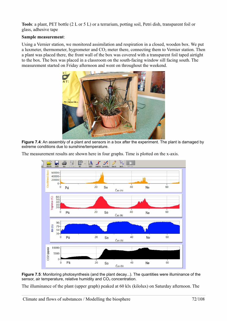
Tools: a plant, PET bottle (2 L or 5 L) or a terrarium, potting soil, Petri dish, transparent foil or glass, adhesive tape

Sample measurement:

Using a Vernier station, we monitored assimilation and respiration in a closed, wooden box. We put a luxmeter, thermometer, hygrometer and CO2 meter there, connecting them to Vernier station. Thena plant was placed there, the front wall of the box was covered with a transparent foil taped airtight to the box. The box was placed in a classroom on the south-facing window sill facing south. The measurement started on Friday afternoon and went on throughout the weekend.

Figure 7.4: An assembly of a plant and sensors in a box after the experiment. The plant is damaged by extreme conditions due to sunshine/temperature.

The measurement results are shown here in four graphs. Time is plotted on the x-axis.

Figure 7.5: Monitoring photosynthesis (and the plant decay...). The quantities were illuminance of the sensor, air temperature, relative humidity and CO2 concentration.

The illuminance of the plant (upper graph) peaked at 60 klx (kilolux) on Saturday afternoon. The

Climate and flows of substances / Modelling the biosphere 72/108

temperature changed with the light; the relative humidity changed with temperature a lot (the water content of the air, much less variable, would be better represented by the dew point of course). The first 24 hours capture the process of photosynthesis (bottom graph). With declining light. the bal-ance between assimilation and respiration changes; more CO2 is released than captured. On Sat-urday morning, with increasing light, photosynthesis started again and the CO2 in air began to wane.But then something unplanned happened. Solar radiation was so intense that the temperature in the box reached 60 ºC, and relative humidity fell from 80 % to 40 %. The plants began to dry up and became a source of CO2. Its concentration rose to around 9 ‰ and remained at that level until Monday morning, when the experiment was terminated. Certainly, some CO2 escaped through the foil by diffusion, so the fact that its concentration remained high implies the continuous production of this gas, which peaked with elevated temperatures in Sunday.

In our experiment, we modelled a global phenomenon that has significant local consequences. Due to climate change, the occurrence and intensity of summer heat waves has increased and will increase further. Under extreme weather conditions, we can witness a so-called “revolt of the plants” appears, when vegetation reduces photosynthesis and becomes a source of CO2. We saw a hint of this in 2003, when western Europe was hit by an extreme heat wave. Trees dried out and the risk of forest fires rose. The weather conditions significantly affect plants and if safe limits are exceeded, the ecosystem can fail. This obviously has serious implications for the lives of people who are dependent on such local ecosystem. The experiment demonstrated not only how the photosynthesis works, but also its limits.

7.2 A question to contemplate: Do we need trees to produce oxygen?The tree, if its biomass and the carbon content of soil underneath it grows, certainly adds oxygen to the air. But is this important at all? We have already dealt with the conversion of carbon dioxide intooxygen and carbon and their re-merging many times, but it will be useful to discuss the situation of CO2 and O2 once more. Suggestions how an “oxygen myth” can be handled in a classroom will emerge from the following discussion.

Oxygen forms a fifth of our air, so per every square meter of the Earth, there are two tons of oxygen. (The weight of the air column above a square meter is ten tons, according to the values of atmospheric pressure and gravity, as you perhaps remember.) Considering this fact, it can be assumed that the amount of oxygen cannot be changed more than negligibly. Oxygen is lost nowhere in nature spontaneously. There is no natural source of carbon, hydrogen of iron with whichit could react.

The Earth's atmosphere originally contained no free oxygen. The predominant compound was carbon dioxide. Together with water, it reacted with calcium and magnesium contained in igneous rocks and created limestone and dolomite sediments, and sediments containing carbonates of calcium and magnesium in general. The total mass of CO2 fixed in such sediments is roughly as large as the mass of CO2 in the atmosphere of Venus (amounting to nearly one thousand tons per square meter), which attests to the similar origin of both planets.

The rest of the once abundant carbon dioxide was then used, over billions of years, by photosynthesizing organisms as a source of carbon for their tissues. The carbon contained in some dead organisms was deposited in sediments. Oxygen remained, a waste product of photosynthesis, with no possibility to react with the carbon hidden in the depths of the continents.

Vegetation adds oxygen to the air even today, but the source for its production, carbon dioxide, is very limited, making not even 1/1000 of our atmosphere. And as some biomass grows, other biomass is decomposed, so that the carbon bonded in organic compounds changes back to carbon dioxide. So the amount of oxygen in the air remains unchanged.

Climate and flows of substances / Modelling the biosphere 73/108

Only when the total biomass on Earth is rising, as it was at the end of the Ice Age and as it is (why?)also now, the amount of oxygen molecules in the atmosphere could slowly change, but over thousands of years it could be no more then say from 20.946 % to 20.950 %... In fact, the reverse process runs now, carbon dioxide is increasing at the expense of oxygen, due to the combustion of fossil carbon. The only problem is the added carbon dioxide, whose amount is not 0.028 % any more, but 0.040 % now, and 0,041 % within next ten years.

The exact amount of oxygen in Earth's atmosphere matters very little. When we walk up to Sněžka (Schneekoppe), the highest Czech mountain, a single breath gives us as little oxygen as if its concentration down in the foothills was just 19 % instead of 21 %. Hardly any organism suffers from such a change. Those who live permanently at a height of up to five kilometres where the partial pressure of oxygen is twice less than at sea, adapt to the situation by maintaining more red blood cells ... it involves many Tibetans and Sherpas, of course top athletes strive for a similar adaptation.

The exact amount of carbon dioxide, on the contrary, is enormously important, as it controls the temperature of the Earth's surface. When the CO2 concentration is constant, so are average temperatures of air and oceans. When carbon dioxide is increasing rapidly, dramatically enhancing thermal insulation of the Earth's surface from the cold space, the climate is rapidly warming. These two processes are tied, now running at a rate ten times faster than at any time in the past hundreds of millions of years.

In the last half billion years, the concentration of oxygen in the air has been one tenth to one fifth. Whereas that of carbon dioxide, during all that time, remained between 2/10,000 and several 1/1000. In the initial gigayears of the Earth's existence it was the other way around. The Proterozoiceon from 2.5 Ga ago to 0.5 Ga ago witnessed oxygen content one to three orders of magnitude lower than at present.

Figure 7.6: Development of partial pressure of oxygen in the atmosphere over the past four billion years. The classic interpretation indicates two step increases in oxygen pressure, this is marked in red. Right axis shows the ratio of the pressure to the present one (Present Atmospheric Level, PAL), left axisis a decadic logarithm of pressure divided by one atmosphere (i.e. 101 kPa). Blue indicates a development that is more in line with new research. For example, it is possible that the oxygen concentration rose from a millionth to something around 1/10,000 several times during the Archaean (pale blue arrows). Changes from the Archaean to Proterozoic and from Proterozoic to Phanerozoic were perhaps quite complicated, as indicated by blue rectangles and curves. Source of image and discussion, see

(Lyons, Reinhard, a Planavsky 2014).

Details of changes of oxygen for the last hundreds of millions of years are still uncertain. Probably, its concentration was mostly lower than today, which would also be line with expectations, because the quantity of sediments containing reduced carbon was growing likely. The source of free oxygen is carbon dioxide from volcanic activity along with water, as photosynthesis changes these compounds to organic ones in which carbon and hydrogen are less oxidized. Deep in sediments, organic matter generally changes to hydrocarbons, in extreme case losing all hydrogen over (graphite). Conversely, a sink of free oxygen exist: volcanic emissions of hydrogen, hydrogen sulphide and carbon monoxide. The amount of oxygen can change by several per cent over millions

Climate and flows of substances / Modelling the biosphere 74/108

Age / Ga

4.0 3.5 2.0 1.5 1.0 0.5 0.0

–5

–3

–1

pO

2/

atm

)

3.0 2.5

Oxygenic photosynthesis

pO

2/ P

AL

100

10–2

10–4

log

(

of years, depending on whether formation of carbonaceous deposits prevails or oxidation of admixtures of volcanic gases (which are dominated by fully oxidized substances, namely water vapour and carbon dioxide, see volcano.oregonstate.edu/book/export/html/151).

Figure 7.7: Comparison of partial pressure of O2 computed from composition of old ambers (red) with older proposed models based on mass balance estimates (Berner 2006) or char contents in sediments (Glasspool a Scott 2010). Source: Figure 12 (Tappert et al. 2013).

In conclusion, let's calculate how much would be atmospheric O2 reduced if all aboveground biomass on Earth would be burned or otherwise oxidized, together with all known deposits of concentrated fossil fuels. Carbon in above-ground biomass amounts to about 0.6 Tt, i.e. 6·1011 t, seeearthobservatory.nasa.gov/Features/CarbonCycle. Fossil deposits are some 0,8 Tt (Hansen, Kharecha, et al. 2013). By forming CO2, carbon would bind oxygen in a mass ratio 2·16/12=2.67, so a bit less than 4 Tt of O2 would be lost. As one square metre of Earth surface has 2 t of atmospheric oxygen over it, loss of 4 Tt would correspond to 2·1012 m2, 2·106 km2 , so to a square with an edge of some 1400 km. This is 0,4 % of Earth surface area (5·108 km2), so the loss of oxygen would be below half per cent of its current amount. Instead of a nowadays concentration 20,95 %, the new one would be 20,86 %... Nobody would notice, the only real possibility to detect it would be, like it is done now, by studying the ratio of N2 and O2, see pages scrippso2.ucsd.edu. But the increase in CO2 content to over 0.1 % would be fatal, not because of our breathing (such concentration prevails most of the time indoors, any problems start with concentrations of more than one or two percent), but due to the sheer transformation of the earth's climate. Complete loss ofaboveground biomass, of course, is not yet conceivable, but the pace of mining the deposits of coal, oil and gas is accelerating and the possibility that the known deposits will be mined completely is an actual threat.

Great climate disruption would certainly prevent mankind from mining even less concentrated accumulations of hydrocarbons, so-called unconventional deposits, and undiscovered reserves of coal. They may contain up to 30 Tt of carbon (Hansen, Kharecha, et al. 2013). But even if burning such a giant amount of carbon, the concentration of oxygen would remain over 19 %. Its partial pressure, relevant for breathing, would fall by about as much as when you move from seashore to highlands. How is it possible that oxygen is simply “indestructible” artificially? This is because the vast majority of non-oxidized carbon is contained in the Earth's crust in a non-concentrated form,

Climate and flows of substances / Modelling the biosphere 75/108

dispersed in common sediments at all continents, there is no possibility to mine it. Such sediments are, e.g., all the mudstones and limestones which are darker due to diffuse carbon, sometimes being almost black.

On the Web, you can meet texts that contain complete nonsense about the oxygen concentration. Like claiming there is much less of it in cities. However, something like that can happen only insidea great fire...

Climate and flows of substances / Modelling the biosphere 76/108

8 Remote sensingRemote Sensing (RS) is a method of exploring the Earth by sensing just radiation from it or by inspecting it by radar or lidar. On the Earth's surface, we can make accurate meteorological measurements, chemical analysis of water and soil, identification of biological species in a certain area, etc. A view from afar does not examine the details of individual objects, but opens up a different perspective. We can see the position of an element (forest, lake, city, ...) in the context of the local landscape and of the entire complex Earth system. Of course it is good to obtain as much information as possible concerning a given site, but collecting data repeatedly over a long time enables to capture important changes. The measured data from some satellites are publicly availableon the Internet in plain text format or in the form of images and animations. A figure sometimes says more than a thousand words or numbers. The usual way of displaying data (visualization) is a map in which a given quantity is shown by a colour from a defined colour range. You could say that remote sensing is the most expensive way to produce a colour picture...

Remote sensing began in the mid-19th century, when the first attempts were made at photographing the Earth's surface from a balloon. In 1903, a patent was granted for miniature pigeon-mounted camera. During World War I, aerial photography was developed. The first picture of the Earth's surface from an orbit was taken by the Explorer 1 satellite in 1958. In 1959, Vanguard 2 satellite was launched, which was designed to measure daytime cloud cover. This satellite scanned the Earthusing photocells and detected the solar radiation scattered by clouds (about 80 %), the land (15 % to20 %) and the oceans (about 5%). Due to problems with the rotation of the satellite, not much useful data were obtained. A real satellite-based remote sensing started with the launch of TIROS-1by NASA in 1960, which produced images of the Earth using two television cameras. TIROS-1 wasthe first successful “weather satellite”, a Television Infrared Observation Satellite.

Individual satellites typically carry multiple devices, each of which has a different task. These devices can be either passive, in that they detect radiation emitted, reflected or scattered by the Earth's surface and atmosphere, or active (radar, lidar), in that they emit electromagnetic radiation and receive modified signals. When measuring the radiation emitted or reflected by the Earth's surface, the atmosphere distorts the signal. At certain wavelengths, the atmosphere is impermeable, while at others, it is more or less transparent (atmospheric windows). The observation of the Earth's surface by satellites is limited by weather conditions, especially cloud cover. Sometimes the atmosphere itself is the object of examination. For example, by utilizing the sunshine reflected fromthe Earth's surface, it is possible to examine the quantity and properties of aerosols.

Classification of orbits of satellites

1. An orbit can be circular or elliptic.

2. Satellites can circle the Earth on various planes. An equatorial orbit is directly above the Earth's equator. A polar orbit passes over both poles. Orbits can be also inclined variously.

3. Orbits are also classified according to their altitudes, as follows:

• GEO (Geostationary orbit), some 36,000 km over Earth surface

• MEO (Medium Earth Orbit) 8.000 – 20,000 km

• LEO (Low Earth Orbit) 500 – 2,000 km

• SSO (Sun-Synchronous Orbit) – see Wikipedia; a combination of proper inclination and altitude up to 5 thousand kilometres is used

• HEO (Highly Elliptical Orbit) – 500 km or less at its nearest point and some 50,000 km at its most distant point

Climate and flows of substances / Remote sensing 77/108

GEO satellites are “geostationary”, i.e. orbit above the equator at the same angular speed as the Earth rotates. Their position on the sky is stable therefore. They are used mainly for purposes radiocommunication (TV) and for meteorological monitoring of certain area (e.g., Meteosat-8). A list GEO satellites is here: en.wikipedia.org/wiki/List_of_satellites_in_geosynchronous_orbit

An example of the use of MEO orbits is a navigation system of 24 GPS satellites. Orbits are inclined at an angle of 55º to the Earth's equator. Four satellites are located on each of six orbital planes separated by 60º. By detecting signal from several GPS satellites, the position of objects on the Earth's surface, of planes and of remote sensing satellites can be precisely determined. GPS is now used by the public without restriction, but it was originally developed for the U.S. Army. For strategic reasons, the EU is currently building its own navigation system named Galileo, which should consist of 30 satellites. The first two ones have been launched in 2011. (The managing administrative centre of Galileo is located in Prague.)

LEO is the most commonly used track for remote sensing satellites, as the entire Earth's surface may be gradually scanned from it. It is considerably cheaper to bring satellites to a low Earth orbit than to MEO and GEO. Solar-synchronous orbit (SSO) are especially convenient for remote sensing, as they allow LEO satellites to fly over a certain latitude always at the same hour (e.g., Landsat-7).

Characteristics of remote sensing systems: (SIC 2012)

Spatial resolution

• high (0,6 m to 4 m) – GeoEye-1, WorldView-2, QuickBird, IKONOS, FORMOSAT-2

• middle (4 m to 30 m) – ASTER, LANDSAT 7, CBERS-2

• low (30 m)

Time resolution (how often a measurement is repeated at the same location)

• high ( 4 d)

• middle (4 d to 6 d)

• low ( 6 d)

Spectral resolution

• high (220 bands)

• middle (4 to 15 bands)

• low (3 bands)

Climate and flows of substances / Remote sensing 78/108

Figure 8.1: Types of orbits of satellites. And also an example of a confusing drawing. The diagram of the very elliptical orbit is inconsistent with the labelled perigee of about 500 km above the ground and of the apogee and the requirement that the Earth has to be in the focus of the ellipse. Source: www.cpi.com/capabilities/ssa.html

Astronauts on the International Space Station ISS photograph the Earth from a height of about 350 km. Unlike automated sensing systems, astronauts have the freedom to decide where to point the camera and when to press the shutter button. Objects of historical, environmental or aesthetic interest are often chosen to be imaged. An archive of photos taken from the ISS is eol.jsc.nasa.gov.

Figure 8.2: Astronaut J. N. Williams (left) when photographing the Earth, and astronaut T. C. Dyson (right) watching down from the International Space Station. From: archive.org/details/HSF-photo-iss013e07989, a en.wikipedia.org/wiki/Iss

A list of weather and remote sensing satellites is en.wikipedia.org/wiki/Nimbus_program. The A-train and GRACE satellilte systems are crucial for studying climate change.

8.1 A-train (Afternoon Train)The US-French project originally planned to incorporate seven satellites on the same orbit for collecting data on the Earth's surface and the atmosphere from the same location only several minutes apart. Today, there are only 6 satellites instead of 7, because OCO and Glory satellites weredestroyed during launch (OCO-2 has been in orbit since July 2014). This set of satellites is LEO, polar, and solar-synchronous. Each of the satellites fly over the equator at about 13:30 local time.

OCO-2 (Orbiting Carbon Observatory) – it measures regional CO2 concentration accurately to identify sources and sinks of CO2 (oco.jpl.nasa.gov).

Aqua (EOS PM-1) – since 2002, it has monitored precipitation,evaporation and the water cycle. Aqua carries 6 instruments:

• AMSR-E — Advanced Microwave Scanning Radiometer-EOS• MODIS — Moderate Resolution Imaging Spectroradiometer• AMSU-A — Advanced Microwave Sounding Unit

Climate and flows of substances / Remote sensing 79/108

Figure 8.3: Scheme of the A-train set of satellites. Glory is still missing. From: en.wikipedia.org/wiki/A-train_(satellite_constellation)

• AIRS — Atmospheric Infrared Sounder• HSB — Humidity Sounder for Brazil• CERES — Clouds and the Earth's Radiant Energy System

CloudSat – since 2006, it has measured the altitudes and properties of clouds by radar

CALIPSO (Cloud-Aerosol Lidar and Infrared Pathfinder Satellite Observations) – since 2006, it has measured aerosols and the emittance of cirrus clouds, using 3 systems:

• CALIOP (Cloud-Aerosol Lidar with Orthogonal Polarization)• WFC (Wide Field Camera)• IIR (Imaging Infrared Radiometer)

PARASOL (POLarization and Directionality of the Earth's Reflectances) – a French satellite lauched 2004. In 2009-2010, it was separated from A-train, its orbit was lowered by 4 km. It carries an instrument POLDER, which measures the physical prperties of clouds and aerosols. It uses both passive and active techniques (radiometer, polarimeter, radar, lidar).

Glory – destroyed 2011 during unsuccessful launch. It was designed to investigate the role ofaerosols in global climate change.

Aura (EOS CH-1) – it orbits since 2004, investigating chemical properties of the atmosphere. It carries 4 measuring systems:

• HIRDLS (High Resolution Dynamics Limb Sounder)• MLS Microwave Limb Sounder)• OMI (Ozone Monitoring Instrument)• TES (Tropospheric Emission Spectrometer)

Climate and flows of substances / Remote sensing 80/108

8.2 GRACE (Gravity Recovery and Climate Experiment)

Climate and flows of substances / Remote sensing 81/108

GRACE is a set of two satellites (nicknamed Tom and Jerry ) on the same orbit polar orbit at an altitude of 500 km. The exact position of the satellites is monitored by a camera shooting the stars, magnetometers and GPS receivers, as well as by using a reflected laser beam sent from ground stations. The distance between the satellites is about 220 km, but it is constantly changing due to thegravity anomalies, including those caused by the Earth's surface features. Using microwave signals between them, Tom and Jerry measure their relative speed and distance with an accuracy of tens of micrometers. GRACE detects changes in ice volume, groundwater and ocean levels.

8.3 Use of remote sensingToday, when people plan a holiday abroad, they no longer consult an atlas of the world. Instead, they connect to the Internet to find all of the necessary information, maps, aerial photographs, photographs, etc. of their destination. Many people use on-line applications, such as www.mapy.cz, maps.google.com, wikimapia.org, etc., which offer fast access to aerial and satellite images of the Earth's surface. These applications require only a standard Internet browser. Google Earth features an intuitive user interface that can be downloaded for free. Google Earth can take you on a detailed tour, 3-D tour of the city of your choice, so you feel as if you yourself were visiting. However, theseapplications are not just for fun. Using Google Earth, archaeologists can find the foundations of buildings under the surface of agricultural land, stone temple ruins in the jungle etc.

Remote sensing data are used by scientists to refine models of global climate change on supercomputers. Geographers use very sophisticated GIS (geographic information system) softwareto visualize and analyse data.

Public access to such data is, e.g., through the NASA Earth Observatory: earthobservatory.nasa.gov.If you wants to handle data directly, you can use databases of many satellite measurements, such as:glcf.umd.edu/data, ftp://e4ftl01.cr.usgs.gov, due.esrin.esa.int/wfa.

8.4 Task: Poster on environmental theme using Remote sensingUsing wikimapia.org (or other tool), find a satellite image of a site where human activity is seriously damaging the environment or where there are clear signs of global climate change. Gather enough information on the chosen topic and create a poster you can present to the class. The satellite image might be supplemented by terrestrial photos, or using on-line RS databases. Your teacher should specify the details (e.g., poster format, method of creating the poster). The poster may be prepared by students individually or in groups.

Climate and flows of substances / Remote sensing 82/108

Figure 8.4: The GRACE satellites (the real distance between them is 220 km). Source: www.satnews.com/cgi-bin/story.cgi?number=34004322

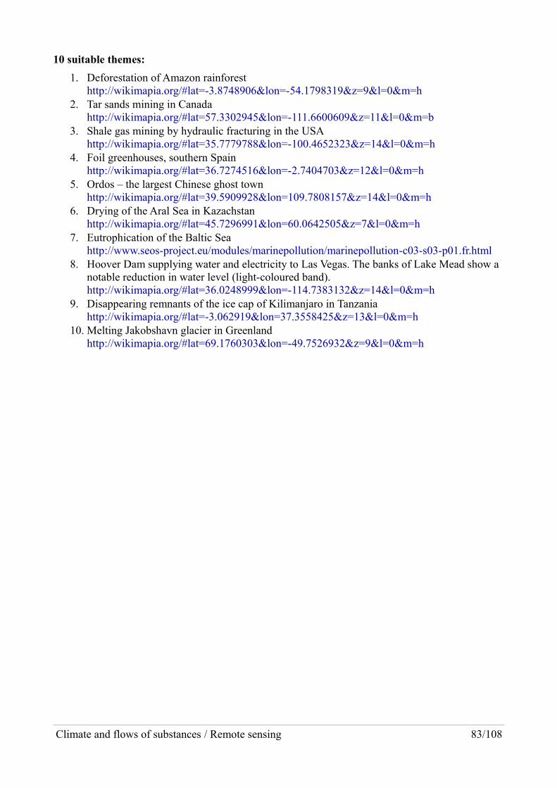
10 suitable themes:

1. Deforestation of Amazon rainforesthttp://wikimapia.org/#lat=-3.8748906&lon=-54.1798319&z=9&l=0&m=h

2. Tar sands mining in Canadahttp://wikimapia.org/#lat=57.3302945&lon=-111.6600609&z=11&l=0&m=b

3. Shale gas mining by hydraulic fracturing in the USAhttp://wikimapia.org/#lat=35.7779788&lon=-100.4652323&z=14&l=0&m=h

4. Foil greenhouses, southern Spainhttp://wikimapia.org/#lat=36.7274516&lon=-2.7404703&z=12&l=0&m=h

5. Ordos – the largest Chinese ghost townhttp://wikimapia.org/#lat=39.5909928&lon=109.7808157&z=14&l=0&m=h

6. Drying of the Aral Sea in Kazachstanhttp://wikimapia.org/#lat=45.7296991&lon=60.0642505&z=7&l=0&m=h

7. Eutrophication of the Baltic Seahttp://www.seos-project.eu/modules/marinepollution/marinepollution-c03-s03-p01.fr.html

8. Hoover Dam supplying water and electricity to Las Vegas. The banks of Lake Mead show a notable reduction in water level (light-coloured band).http://wikimapia.org/#lat=36.0248999&lon=-114.7383132&z=14&l=0&m=h

9. Disappearing remnants of the ice cap of Kilimanjaro in Tanzaniahttp://wikimapia.org/#lat=-3.062919&lon=37.3558425&z=13&l=0&m=h

10. Melting Jakobshavn glacier in Greenlandhttp://wikimapia.org/#lat=69.1760303&lon=-49.7526932&z=9&l=0&m=h

Climate and flows of substances / Remote sensing 83/108

9 Expressing quantities9.1 Main principles of scientific languageEstablishment and development of towns and trade (within Nile and Indus some 6 ka ago already) led everywhere to the emergence of different ways of expressing quantities and measures. An enormous amount of units were created by different cultures, especially for three variables: length, volume and weight. Early on in history, numerical values for these variables (numerical value = the value of the variable divided by a selected unit) were expressed, e.g., in Babylonian sexagesimal system. This system is still used nowadays when we express time and angles. Ancient way of counting in dozens survived well into the 20th century in Czechia and other countries (a larger quantity 12·12 = 144 is named gross in English, 5·12 = 60 is half small gross, named conveniently kopa in Czech and Shock in German). Counting based on halving (i.e. ½, ¼, 1/8) is commonly used in countries measuring in inches, and in specifying the volume of beverages, such as, for example wine in Austria.

The decimal system won out long ago over the unwieldy Roman numeral system, and the number of zero was introduced. It became easy to express even values that differed by many orders of magnitude by using and writing powers of ten. Such expressions are semilogarithmic – using just the integer part of a decadic logarithm, or the exponent of 10, we can express an order of magnitude, and the “leftover change” within that order is then expressed explicitly. Such numbers are then added together easily, even in your head, such as, for example, 3.45·106 plus 6·104, with a result of 3.51·106.

Units are still not completely universal in our time. The English-speaking world is to blame, as it uses units that predate the French Revolution. One of the reasons may be that the names of such units consist of one syllable. Saying inch, foot, yard and mile instead of the decimal centimetre, metre, kilometre is convenient. Inch, foot and yard are comfortable for use in everyday life, as our bodies are their “standards”. But for accurate measurements, or those far outside human dimensions(such as thousands of feet for aircraft altitudes), this advantage disappears. In Czech common spoken language, both centimetre and kilometre can be expressed using two syllables only (cenťák and kilák, respectively). The same goes for kilogram or decagram (kilo and deka, the latter being used when buying food instead of asking for tens or hundreds of grams). All of these shortened versions refer to just the prefixes, i.e. order of magnitude; the actual unit of measure concerned can be understood based on the context of the situation. Thanks to that the pre-metric units are no more used in Czechia, with an exception of piping and plumbing fittings (here the German Zoll, sayed coul in Czech, meaning the same as palec, thumb, may live forever, being identical to inch, 25.4 mm). The advantage of English units consisting of one syllable is counterbalanced by the non-decadic conversion between different units, which is rather difficult. Things can be further complicated by the fact that sometimes the same name is used for units concerning different amounts or even completely different things. For example, the English “ton” may mean not only thetwo values of mass around one ton, but even a unit of volume... The name mile has a legitimate meaning, which will persist as long as the sexagesimal angular scale will be used. It is the average length of one minute of arc on the Earth's meridian, which is a very practical unit in aeronautical and maritime navigation. It amounts to 1852 m. English-speaking people, however, have to call it “nautical mile”, as by a single word “mile” they mostly mean 1609 m. The derived unit of speed, nautical miles per hour, is called knot. It is a very convenient unit of speed, as it is one-syllable and easy to convert to a metric unit, being just 3 % larger than 0.5 m/s (so 20 kn rounds to 10 m/s etc.).

When handling just a few orders of magnitude, it may be preferable to avoid the use of numerical semilogarithmic expressions; instead, prefixes can be used as needed. Everyday ones like deci-, deca-, centi-, hecto- (this last one is only used with litre or are in a shorted form hectare) and milli- and kilo-, are supplemented by those which always indicate three decadic orders of magnitude more

Climate and flows of substances / Expressing quantities 84/108

or less: micro-, mega-, nano-, giga-. Hopefully, everyone is familiar with them. The prefixes pico-, tera- and others that express further powers of 1000 are probably less understood, but even peta- and exa- are common in scientific and technical language. They are easy to get used to, if you often encounter them in practical situations. They are unusual but might be convenient even in a realm of finances. Writing or saying that the price was 8 G€, eight gigaeuro, treating symbol of euro as an ordinary unit, is unequivocal. Formulating it as “eight billion euro” may confuse, as it probably means eight milliard euro. It is shorter and unambiguous. In countries where the term milliard is used, it is preferable to avoid billion altogether, replacing it by the prefix tera-.

Confusion in units reigns worldwide, particularly in business, due to the influence of English-speaking countries. Business, unfortunately, uses its gibberish. However, in official documents or inschools and educational texts, such gibberish should never appear outside footnotes mentioning its existence and relation to standard units. Not only it is unnecessary, but it is also confusing. It hinders understanding, and the mutual respect and trust between different disciplines. Instead, it is appropriate and should be mandatory to use the coherent SI standard system originally published in 1960 and maintained and updated since (see en.wikipedia.org/wiki/SI).

Publications by BIPM and NIST, the most important institutions striving to overcome the “medievalepoch” of science and technology, ot only the define units, but the whole way in which quantities should be expressed (BIPM 2006a) (Thompson a Taylor 2008a). Such a proper way is easy to lean. In fact it is much easier than, say, learning Czech orthography, let alone grammar. For a start, it maybe sufficient to master the rules contained in the BIPM's four-page summary (BIPM 2006b). Learning this system is advantageous as no matter what language you are using, quantities are expressed in the same way. Violating the rules of scientific and technical quantitative world “language” for expressing quantities not only reduces clarity, but it sometimes leads to mistakes andconfusion. This unfortunately happens in the study of flows of substances and climate change. Gibberish that is in conflict with scientific language has penetrated even the foremost journals and IPCC reports.

The most egregious excess of that gibberish is mixing chemical symbols with units, sometimes in particularly confusing contexts. Consider the sentence: “Annual CO2 emissions from fossil fuel combustion and cement production were 8.3 [7.6 to 9.0] GtC yr–1 averaged over 2002–2011.” (written at top of p. 10 of Summary for policymakers of the volume Physical science basis of the Fifth Assessment Report of the IPCC) (Stocker et al. 2013).35 What does this scrum “GtC” mean? If there would be a space before C, it would denote coulomb, a unit of electric charge, but we would not expect electric charge in the above sentence. In reality, the authors wish to convey the fact that annual atmospheric emissions (in gaseous form, which is carbon dioxide ultimately) was about 8 Gtof carbon that was previously bound in fossil fuels or carbonates. If we were to take their wording literally, we would have to accept a model where tC is a new unit of mass, amounting to 3.67 t. Thisis because the mass of CO2 emissions is, due to the atomic masses of carbon and oxygen, (12+2·16)/12 = 11/3 of the mass of carbon contained in those CO2 emissions. It would be, however, an absurd and unnecessary unit. In fact the authors, in order to “save” space, have tried to “smuggle” a part of their communications into an expression that should be a mathematics-physics formula, containing only numbers and mathematical symbols, which include unit symbols. A ton is always the same, regardless of whether it is ton of feathers, corn, sugar, water or carrots. Balance scales hold goods (any goods) in one pan and standardized metal weights in the other one; just their masses are compared, not qualities.

35 We do not object to the use of square brackets here; they are used in a very good way. As stated on their first occurrence on page 3 of the Summary, they contain an interval within which the true value should lie with a probability of 90 %. Such a mode of expression, as an addition to the mean or most probable value, can be highly recommended, especially when reporting just standard uncertainty would not reflect well a non-symmetric shape of probability density function or when this function differs from normal distribution.

Climate and flows of substances / Expressing quantities 85/108

The BIPM recommendation for how to express values of quantities reads: “The value of a quantity is expressed as the product of a number and a unit”. Common rules of algebra apply to here (“BIPM– Expressing Values of Quantities” 2006). The NIST explicitly highlights an unacceptability of inserting any additional information in an the algebraic formula expressing value: “When one gives the value of a quantity, any information concerning the quantity or its conditions of measurement must be presented in such a way as not to be associated with the unit”. An example from NIST publication SP811 (Thompson & Taylor 2008b) (for further examples, see there):

the Pb content is 5 ng/L but not: 5 ng Pb/L or 5 ng of lead/L

Let us point out one other offence, also commonly found even in scientific journals unfortunately: between a number and a unit symbol, there must be a space. The only exception are symbols expressing a sexagesimal planar angle unit (degree, minute or second), see section 7.2 Space between numerical value and unit symbol in the repeatedly referenced NIST publication, physics.nist.gov/Pubs/SP811/sec07.html#7.2. In Czech it may be acceptable to write symbol % without being preceded by a space, if it is not an expression of a quantity, but an adjective (e.g., “10% zvýšení”, “desetiprocentní zvýšení”); this, however, is not possible in English, as such an adjective must be written out as a compound noun as ten-percent increase. More on the use of the percent symbol, ppm36 and so on, see section 7.10 of the repeatedly referenced book Guide for the Use of the International System of Units (SI). A blunder from this realm is, e.g. adding any index to a symbol ppm, like explaining that it is a millionth of volume. Appeals to the IPCC to use the correct scientific language, see, e.g. (Hollan 2013, 2014).

Finally, a note about using fonts to distinguish between symbols of quantity and units: variable is tobe written in italics, unit in upright font. This holds even in passages that are otherwise wholly italicised.

We tried to follow the above rules in our book and comment those rare cases when they are broken, as in figures taken from others.

9.2 Visualisation: gnuplot and InkscapeTo understand a dependence of one variable on another one, or to compare several variables, except in trivial cases, graphic methods should be used. A graphic approach can be employed to quickly find the answers to questions such as “When does this variable reach the selected value?”. Even before the era of desktop computers, it used to be quicker to sketch a graph and find an approximateanswer than to embark on a mathematical solution. Now the creation of graphs has become quite easy. Many people use spreadsheets like Microsoft Excel or its OpenOffice or LibreOffice counterparts, for handling tabulated data. The program gnuplot offers many more options and can work faster with various data and mathematical formulas. Text files are used for input data, as human-readable text is the only reliable data storage format that can be read at any time regardless of the software. Data stored in complex formats can be always exported as plain text files. Text datacan be freely interspersed with notes; such comment lines start by the # symbol and gnuplot will ignore them when loading data. The graphs in this book are mostly created this way, using, e.g., text files available from the websites of American scientific institutions. The source programs (or “scripts”) for gnuplot are stored in the directory amper.ped.muni.cz/gw/activities/graphs/sources/. Hollan, Miléř & Svobodová (2013) contains further references.

As with all programming, the easiest way to start is to take an existing program, and simply modify it for one's own use, e.g., by just changing the output to a SVG format instead of PDF (for examplesof alternatives to both formats see the above-mentioned directory). Graphs in SVG format are concise; you can include them directly into documents using OpenOffice or MSWord. The format is

36 The Guide recommends to avoid using units (symbols of numbers) ppm, ppb, ppt, as they are language-specific (and of course, ppb assumes that billion is 109). However, for atmospheric concentration of CO2, units ppm can be regarded as indispensable and becoming understood universally. We use them in our book, unlike ppb.

Climate and flows of substances / Expressing quantities 86/108

supported by web browsers, but the “typesetting” of exponents, indices, etc. may not display correctly. The only safe bet is using PDF format, from which a bitmap in PNG format can be produced by simply copying a rectangular part of the screen with any PDF reader (Acrobat Reader, Foxit, ...). For including a bitmap in any document, unless it is a photo, PNG is the only suitable format; the same is true for graphs that are displayed directly in web browsers like Firefox. However, if it is a very simple graph, SVG vector format is preferable, as it provides unlimited resolution.

Changing of labels contained in a graph can be done either by editing the source code for gnuplot, or using a drawing program Inkscape, inkscape.org. This tool can be used to create other language versions of images in vector format (EPS, AI, PDF, SVG, WMF, EMF) and save them both in vector form and as a PNG bitmap. (To get a proper bitmap, it may be necessary to set background colour as white, by selecting File – Document Properties – Background and entering 255 in registry A). Inkscape is capable of creating high quality PDF output, which, until recently, was only possibleusing Adobe Illustrator, a commercial program, which is not available for the Linux platform. Newer graphs in our book, if they were taken from elsewhere, were modified using Inkscape.

Both gnuplot and Inkscape can run on all of today's operating systems, and their use in the future is assured due to the fact that these programs are open-source programs, maintained and developed by a large community of expert users. Learn to use them.

One of the easiest ways we can recommended to start using these programs, is correcting poor labels of axes of graphs. If an axis has mere numbers by its ticks, i.e., numerical values of a quantity, the description of the axis has to be formulated so that the result of the given algebraic expression is just a number. This is an easy task; the quantity has to be divided by the appropriate unit. The unit is written following a slash mark. This approach is absolutely necessary if the axis shows a logarithm of a dimensional quantity – the argument of a logarithm cannot be anything else besides a number. A clumsy, flawed, and unfortunately common way to indicate what the author actually means by the displayed numbers, is to place the unit into brackets, as if it were a comment. Please, never describe graphs in this incorrect fashion. (This applies also to the authors of this book.We all have something to learn). See the very beginning of Chapter 7 of the repeatedly cited publication NIST SP811, physics.nist.gov/Pubs/SP811/sec07.html.

Climate and flows of substances / Expressing quantities 87/108

Glossary(Absolute) Black body, black emitter, blackbodyA theoretical object that absorbs all incident radiation. Such an object then emits electromagnetic radiation (radiates due to its temperature) according to Planck's law and the Stefan-Boltzmann law; the amount and spectrum of emitted radiation is a function of the absolute temperature only. A good practical realization of a blackbody is a small hole in a large cavity in a solid opaque object. A large-area approximation of a blackbody would be a the system of black fibres standing upright on asubstrate, like a velvet. Natural surfaces with rich structures, such as grass or forest, behave like black bodies to longwave infrared radiation.

EmittanceEmittance (or emittivity) is the ratio of radiant flux emitted from the sample surface to that from a same-sized blackbody at the same temperature. It is therefore a property of an object. If the object ishomogeneous, impermeable to radiation and the sample surface is smooth, then its emittance is identical to emissivity, which is a material property. Emittance and emissivity can attain values from0 to 1 (1 applies to a black body). If it does not attain these extreme values, directional emittance can be specified: the radiation from the sample surface can have different radiance in different directions, unlike that from a black body. The same holds true for spectral emittance, which is related only to a specific wavelength, or even a specific direction (directional spectral emittance). Emittance varies somewhat according to the temperature of the object. On one hand, this is because a higher temperature equates to a larger proportion of short wavelength radiation, and on the other, this is because large temperature changes transform the material properties of the object.

Photopic spectral sensitivitySensitivity of human vision underconditions with ample light, accepted asa convention. In the figure at right it isplotted at a logarithmic scale. From 500nm to 610 nm it remains above half ofthe maximum. Source: Luminousefficiency functions, 10-deg function (Stockman 2007).

LuminanceA quantity, which is the base of a visualsensation. It is an amount of lightincident on a given surface from a givenspace angle (i.e. from the correspondingpart of the observed scene), divided bythe area of that surface and by that spaceangle. Its unit is candela per metresquare, this being the same as lumen permetre square and steradian. As all phtometric quantities, luminance can be derived from energy quantities. In this case from the spectral radiance, using the conventional spectral sensitivity of human vision – luminance is an integral of their product.

Luminance is, as far as photopic, or daytime (colour) vision is concerned, a rather abstract quantity;our vision can compare luminances of two objects reliably only if their colour is the same. To compare visually whether a blue, green or red object has a higher luminance is is a more difficult task; a full quantitative description of luminous properties of an element of space angle needs a trio or a quartet of values akin to luminance, taking into regard spectral sensitivities of the corresponding types of light-sensing cells of the retina. In case of nocturnal vision void of colour

Climate and flows of substances / Glossary 88/108

recognition, the situation is simpler, but the adequate quantity is a scotopic luminance, which is calculated based on spectral radiance useing another kind of spectral sensitivity of vision, shifted towards shorter wavelenthgs.

ClimateThe aggregate properties of weather over some period. Climate is described statistically, e.g. by frequency distribution of various values of a chosen quantity. Or more simply, by selected parameters that describe such a distribution (mean, median, various percentiles). Most commonly, temperatures are studied this way. Apart from a frequency distribution of a given quantity, the pace of the said quantity's change from one day to another day, or the range between daytime and night values properties needed for describing the change of weather over time, such as statistic of abrupt changes in weather (Wettersturz in German). For precipitation not only are daily, weekly, monthly and annual totals important but so are five-minute maximum values. The aim of the studying the climate is to understand changes in biosphere, hydrosphere and cryosphere, as well as changes in the surface of the continents, which together with atmosphere form the climate system. Therefore, phenomena such the evaporation rate or total evaporation from an area are climatic quantities too, which together with total rainfall and total runoff determine conditions in the landscape. Most generally, the climate can be understood as a state of the climate system, over a given area, which may be as small as just a few meters or as large as the whole Earth, taken in a given time or as a statistics for the period up to decades or centuries.

In German, the aggregate of the weather properties of a small area for shorter periods of time (ranging from a few days to an entire season) is called Witterung. Properties of weather within such time interval develop influenced by other regional components of the climate system – the albedo ofland is essential for solar radiation, evapotranspiration (the evaporation of water from moist surfaces and through stomata of plants), and, vice versa, water condensation in the form of dew or frost on surfaces which cooled down sufficiently by radiation from dusk until dawn.

The term climate is derived from the Greek klinein, which can be translated as a slope („What exactly is the climate?" 2010). This slope refers to the angle at which solar rays are incident to the Earth at different latitudes at noon; at the equator, they fall almost vertically to the ground, whereas at high northern latitudes they are very slanted. Around the winter solstice, the angle of incidence is much larger in the high north than around the summer solstice, if the Sun appears at all. When the incidence of solar rays is oblique, solar radiation with a flux density of 1 kW/m2 spreads over a larger area of the Earth's surface; the surface irradiance is equal to the solar radiant flux density multiplied by the cosine of the angle of incidence. Due to this, at high northern latitudes the sun warms a horizontal surface much less than in the tropics.

This fact makes the existence of climate zones possible. These zones differ not only in average temperatures but also by the amplitude of temperature changes over the year, between seasons. The reason for this is simple: there are large changes in the solar heat incident on the earth in a single day, outside tropics. The angle at which the sun shines on the ground changes, as well as the length of time the Sun is in the sky. A second factor that makes the climate of different latitudes even more different is the large-scale circulation of the Earth's atmosphere. In areas where air sinks down fromlarge altitudes, cloudless weather with very low water vapour content in the air prevails; this namelyconcerns areas of desert in subtropics. And in all latitudes the climate varies according to the distance from the ocean taken in the direction of the prevailing airflow. As a consequence, a truly temperate climate does not cover the whole belt between the tropics and the polar circles: deep inland a continental climate prevails, with less vapour in the air and with large fluctuations in temperature.

For more, see Climate article on Wikipedia.

Climate and flows of substances / Glossary 89/108

IlluminanceThe flux of light incident on a given surface, divided by the area of that surface. It is therefore expressed in units of lumen per square metre, referred to as lux.

IrradianceThe flux of electromagnetic radiation incident on a given surface, divided by the area of that surface. Its unit is, therefore, watt per square metre. In reality, that radiation is measured just over a limited interval of wavelengths, mostly including UV, visible and IR radiation only. It refers to theirradiated surface. A term like Solar normal irradiance would refer rather to the source of radiation, the surface being oriented directly toward the Sun, and would be equivalent to Solar radiant flux density. (An analogous quantity, describing not the incident radiation, but the radiation outgoing from a surface, is called radiant exitance.37)

InsolationAn integral of solar irradiance over a time interval. Its basic unit is, therefore, joule per square metre, but for integrals over one hour (hourly insolation) or the whole day (daily insolation), expressing it in kWh/m2 may be more convenient; this is because clear-sky solar horizontal irradiance of the ground by the Sun near zenith is one kilowatt. Irradiance and insolation of surfacesat the bottom of atmosphere varies with weather. The same quantities for a horizontal surface abovethe atmosphere behave much more simply, depending on the geometry and on the little varying “solar constant”.

WeatherThe local state of the atmosphere and of the processes within it, including a time course of changes of the state of the atmosphere. This complex local state may be valid for a given moment or for a timespan up to several hours. During a 24 h cycle, it varies inevitably as the insolation of landscape changes. (Insolation varies everywhere outside the poles.) More see Wetter and Weather on Wikipedia.

Weather situationThe regional state of the atmosphere and of the processes within it, which may be momentaneous orrelated to a period of up to one day.

PyranometerAn instrument with a heat sensor measuring the input power dueto sunshine. “Pyr” is Greek for fire, and “ano” is the word for“above” or “heaven”. In order to measure total solar radiationonly (from one half-space), it is usually covered with an “acrylicglass” (PMMA) dome. The dome lets no longwave infraredradiation of the air pass through while not suppressing the solarradiation incident on the sensor from low angular heights.

The “opposite” apparatus is a pyrgeometer which features(usually flatter) dome of silicon, which is impervious to solarradiation but lets longwave infrared radiation of wavelengths from 5 μm do 40 μm through rather well. Of course, both devices, when mounted bottom up, can also measure radiation from the ground upwards – reflected solar one or that radiated by Earth's surface.

37 Unfortunately, term exitance is sometimes replaced by “emittance” in this name; this produces a problem when speaking about a very different quantity named emittance, as we use it in this book.

Climate and flows of substances / Glossary 90/108

ReflectanceThe proportion of incident radiation that an object returns back to the half-space from which it came. It may have values from 0 (for a black body or a completely transparent object) and 1. For real objects, reflectance depends on the angle of incidence of radiation on their surface. For the most common case of solar radiation, the reflectance is referred to as albedo. Albedo can differ greatly from the reflectance of longwave infrared radiation (e.g. snow albedo is 0.9, while its reflectance of longwave IR is less than 0.1).

Radiation due to temperature, temperature radiationEmission of electromagnetic radiation by a substance due to the fact that it has a non-zero absolute temperature. As the absolute temperature of all substances is greater than 0 K, temperature radiationis ubiquitous in the universe. How much a substance emits at a particular wavelength depends on itstemperature and also on how much absorbing is that substance at the given wavelength. An object that absorbs all radiation incident upon it (is so-called “absolute black” with an absorptance equal to 1) emits maximum achievable radiant power at a given temperature. The radiant flux per unit area of such a blackbody is given by the Stefan-Boltzmann law, according to which it is proportional to the fourth power of the absolute temperature. The spectrum of that radiation, or howmuch of the radiant flux is emitted at different wavelengths, namely a variable called spectral radiance, is then given by the Planck's radiation law. Real objects do not absorb any wavelength of radiation perfectly, absorptance values are between 0 and 1. For thermodynamic reasons, absorptance is identical to emittance, the ability to radiate due to temperature (otherwise, a warm object could be further warmed up by a cooler object), thus emittance valuea are also between 0 and1. Taken for single wavelengths, we are talking about spectral emittance. Temperature radiation at agiven wavelength is the product of the Planck's radiation function and spectral emittance.

In Czech there is a simple name for such emission process, “sálání”. Even though it is one of the most basic processes in our world, English is lacking a suitable short name for it. Calling it “thermalradiation” is common, suggesting that the radiation is emitted thanks to the fact that the substance iswarm. Unfortunately, such a term also leads to misunderstanding that some radiation might exist that would not convey heat from an emitting object to its surroundings, but this is impossible, as all

Climate and flows of substances / Glossary 91/108

Figure 1: The relative spectral sensitivity of common thermopile pyranometers (red) and pyrgeometers (pink}. For most of sunshine, pyranometer sensitivity is independent on wavelength. Solar spectral irradiance in wavelength domain is plotted schematically, divided by a maximum, which is about 550 nmin this domain. Source: Kipp & Zonen. For an accurate solar spectrum see Figure 3.

radiation is an energy flux that differs from performing work,38 so the sum of radiant energy that travels through a surface within some interval of time is heat.

Greenhouse effectA physical process in which the surface of the planet gets temperature radiation not only from the Sun, but also from the air. The underlying principle of the greenhouse effect is that the atmosphere is more permeable to solar radiation (i.e., radiation with wavelengths mostly below 3 μm) than to the radiation of the Earth's surface and of the atmosphere itself (radiation with wavelenghts mostly above 3 μm, which can be called longwave infrared). In the case of an actual greenhouse, longwave infrared temperature radiation to the ground comes from the glass or other material permeable to sunshine, by which is the greenhouse covered.

Glass is completely opaque for radiation with a wavelength over 3 μm, no such radiation can get through any glass. A thick layer of cloud blocks such radiation completely too. Cloudless atmosphere lets some radiation of wavelengths over 3 μm pass through, but at most of the longwaverange it is rather opaque. E.g., radiation with wavelength of 15 μm is all absorbed on a path of just one kilometre.

The ability to absorb and emit radiation is due to the admixtures of air, known as greenhouse gases:water vapour, carbon dioxide, methane, nitrous oxide, and even ozone – always molecules with more than two atoms. The proportion of water vapour in the air depends on its temperature, over warm oceans the amount of water in air is much higher than over cold oceans. And upward, due to temperature decrease with height, concentration of water vapour decreases rapidly, in the stratosphere its content is incredibly low. Durability of water vapour in the air is a few days, because when the air is cooled sufficiently, vapour promptly disappears in the form of liquid or solid precipitation. The share of other greenhouse gases except ozone is little variable within the troposphere, we name them well-mixed gases; this results from their many-year lifetime in the air.

38 Work is such transfer of energy through a system boundary, which can be expressed as the integral of the product oftwo observable quantities, such as force and displacement or voltage and current. Heat can be considered to be the sum of innumerable cases of “microwork” at the molecular to subatomic level; due to the quantum nature of such events, however, heat cannot be calculated the same way as work. On the other hand, it is true that the photons of visible and UV and IR ranges can, in special electrical systems, exert individual cases of microwork, the sum of which can be calculated directly as electric work; photovoltaic cells are based on this principle. But even such a process can be considered to be a special quantum thermal process where the heat source is very hot Sun. For more on physical quantities and energy units, see amper.ped.muni.cz/eave/veliciny.pdf (in Czech).

Climate and flows of substances / Glossary 92/108

Figure 2: A scheme of greenhouse effect and radiative forcing of long-lived greenhouse gases. The total of longwave (>3 μm) infrared radiation near the ground is much larger than solar input; downwelling IR emitted by the air is almost twice larger than solar radiation, taken as an average over the globe. Thanks to that the average Earth surface temperature is about 15 ºC. Longwave radiation to the space comes mostly from high layers of the atmosphere, which are very cool. Due to increased concentration of greenhouse gases, the height from which this outward longwave radiation comes, shifted still higher, to even cooler air. Warming of the Earth will stop only after even these higher layers attain such temperature, that their emission to the space will be the same as the sum of the absorbed solar radiation.. (The radiative imbalance of 3 W/m2 shown in the chart would hold for a non-real case when no cooling aerosols would be produced by mankind and the air would be no warmer then centuries ago.) Source: amper.ped.muni.cz/gw/obrazky/warmin_en.eps. A larger illustration with a lot of text is at the end of our book.

To compare how much emissions of different gases contribute to warming, a variable called Global Warming Potential, GWP has long been used. For CO2 it is 1, for methane and nitrous oxide it is by orders of magnitude more, for halogenated hydrocarbons again so. It refers to the same mass of emissions. As a rule, we evaluate what will be an integral of radiative forcing attributable to emissions particular gas emissions compared to the same mass of carbon dioxide, taken for a periodof one hundred years (centenial warming potential, GWP100). For CH4, it is conventionally 28, for N2O, it is 265. But methane emissions which oxidize within few years to CO2 and H2O, have a far greater relative warming effect in the short term; for example, over 20 years, methan has GWP20 of about 84. That this is, of course, per gram, not per molecule – 1 g of methane has (12 + 32) / (12 + 4) = 4.11 = 2.75 times more molecules than 1 g of carbon dioxide – even scientific articles confuse that sometimes. In addition to GWP, Global Temperature Potential, GTP is now also used as a better metrics to describe the temperature impact of the emissions after a given number of years from those emissions. This is not much different for nitrous oxide, which remains in the atmospherefor many decades, but for methane it is much lower, its GTP20 being given as 67, GTP100 as only 4. See chapter 8.7 of Physical Science Basis (Myhre et al. 2013).

Climate and flows of substances / Glossary 93/108

Solar spectrumcontains a very wide range of radiation wavelengths. For the Earth's temperature only a part of it is essential – that one which accounts for the vast majority of the energy flux, which is the range from 200 nm to 4 μm. The crucial quantity is the power density in an average distance of the Earth from the Sun. The relevant quantity is called the spectral radiant flux density. After passage through the atmosphere, radiation is substantially attenuate in several bands infrared spectrum by water vapour. Vapour the content in the atmosphere is however very variable, depending mainly on the temperature of air.

Spectral radianceRadiance attributable only to a small wavelength interval, divided by the size of the interval. Or, similarly to the interval of frequencies of electromagnetic radiation. The basic unit is, in the first case, watt per metre cubed and steradian.

Figure 3: The red curve shows the spectral radiant flux density of solar radiation at a distance of 1 AU from the Sun. At the top of the scale, wavelengths at which the solar photosphere (the layer where radiation leaves to space) strongly absorbs, due to hydrogen, sodium and calcium. As a consequence, dark features in the spectrum appear, called spectral lines (some other, even darker, are caused by ironand magnesium). Spectral line labelled O2, in the description the most right one, arises in the Earth's atmosphere. From this line to the left, till the (double) line of calcium, the visible light region spans. Its spectrum was first described by Fraunhofer who denoted the marked lines by the letters A, C, D, F, G, H and K. Script: amper.ped.muni.cz/gw/aktivity/graphs/sources/sol_eng.gnp

The area under the red curve in Figure 3, i.e. integral of the curve is equal to the solar constant, 1361 W/m2. The smooth curve shows a spectrum of a blackbody at the place of the Sun, if it would have the same radiant output. The temperature of such a body is then the effective temperature of the Sun. In those places of spectrum where the Sun shines more a blackbody with such temperature,we observe radiation from lower, warmer layers of the photosphere. On the contrary, the wavelengths at which the Sun shines less than such blacbody, come from the highest, coolest regions of the photosphere. From which depth of photosphere some radiation comes, that depends on the transparency of the photosphere for a given wavelength.

At the bottom of the Earth's atmosphere, sunshine is weaker. Two processes are a cause. First, even a cloudless atmosphere scatters part of the radiation back into space. Second, some infrared

Climate and flows of substances / Glossary 94/108

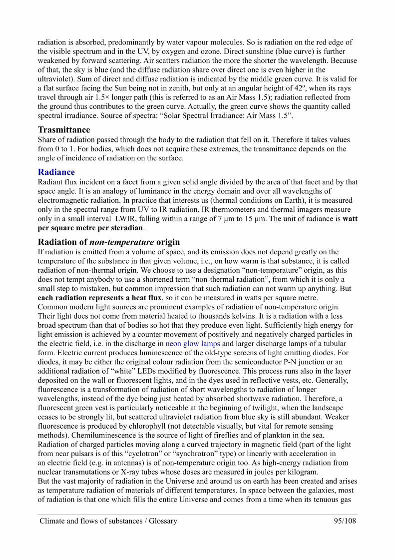
radiation is absorbed, predominantly by water vapour molecules. So is radiation on the red edge of the visible spectrum and in the UV, by oxygen and ozone. Direct sunshine (blue curve) is further weakened by forward scattering. Air scatters radiation the more the shorter the wavelength. Becauseof that, the sky is blue (and the diffuse radiation share over direct one is even higher in the ultraviolet). Sum of direct and diffuse radiation is indicated by the middle green curve. It is valid fora flat surface facing the Sun being not in zenith, but only at an angular height of 42º, when its rays travel through air 1.5× longer path (this is referred to as an Air Mass 1.5); radiation reflected from the ground thus contributes to the green curve. Actually, the green curve shows the quantity called spectral irradiance. Source of spectra: “Solar Spectral Irradiance: Air Mass 1.5”.

TrasmittanceShare of radiation passed through the body to the radiation that fell on it. Therefore it takes values from 0 to 1. For bodies, which does not acquire these extremes, the transmittance depends on the angle of incidence of radiation on the surface.

RadianceRadiant flux incident on a facet from a given solid angle divided by the area of that facet and by thatspace angle. It is an analogy of luminance in the energy domain and over all wavelengths of electromagnetic radiation. In practice that interests us (thermal conditions on Earth), it is measured only in the spectral range from UV to IR radiation. IR thermometers and thermal imagers measure only in a small interval LWIR, falling within a range of 7 μm to 15 μm. The unit of radiance is wattper square metre per steradian.

Radiation of non-temperature originIf radiation is emitted from a volume of space, and its emission does not depend greatly on the temperature of the substance in that given volume, i.e., on how warm is that substance, it is called radiation of non-thermal origin. We choose to use a designation “non-temperature” origin, as this does not tempt anybody to use a shortened term “non-thermal radiation”, from which it is only a small step to mistaken, but common impression that such radiation can not warm up anything. But each radiation represents a heat flux, so it can be measured in watts per square metre.Common modern light sources are prominent examples of radiation of non-temperature origin. Their light does not come from material heated to thousands kelvins. It is a radiation with a less broad spectrum than that of bodies so hot that they produce even light. Sufficiently high energy for light emission is achieved by a counter movement of positively and negatively charged particles inthe electric field, i.e. in the discharge in neon glow lamps and larger discharge lamps of a tubular form. Electric current produces luminescence of the old-type screens of light emitting diodes. For diodes, it may be either the original colour radiation from the semiconductor P-N junction or an additional radiation of “white” LEDs modified by fluorescence. This process runs also in the layer deposited on the wall or fluorescent lights, and in the dyes used in reflective vests, etc. Generally, fluorescence is a transformation of radiation of short wavelengths to radiation of longer wavelengths, instead of the dye being just heated by absorbed shortwave radiation. Therefore, a fluorescent green vest is particularly noticeable at the beginning of twilight, when the landscape ceases to be strongly lit, but scattered ultraviolet radiation from blue sky is still abundant. Weaker fluorescence is produced by chlorophyll (not detectable visually, but vital for remote sensing methods). Chemiluminescence is the source of light of fireflies and of plankton in the sea.Radiation of charged particles moving along a curved trajectory in magnetic field (part of the light from near pulsars is of this “cyclotron” or “synchrotron” type) or linearly with acceleration in an electric field (e.g. in antennas) is of non-temperature origin too. As high-energy radiation from nuclear transmutations or X-ray tubes whose doses are measured in joules per kilogram.But the vast majority of radiation in the Universe and around us on earth has been created and arisesas temperature radiation of materials of different temperatures. In space between the galaxies, most of radiation is that one which fills the entire Universe and comes from a time when its tenuous gas

Climate and flows of substances / Glossary 95/108

fill at temperatures of thousands of kelvins became sufficiently transparent; expansion of the Universe lengthened the waves of that ancient radiation so that now this “background radiation” or “relic radiation” has a same spectrum as a substance at 3 K would emit.

Sudden weather change (Wettersturz)Quite a large and sudden change of the weather situation. Some weather twists causeg serious prob-lems to people, infrastructure, agriculture, etc.

Climate and flows of substances / Glossary 96/108

SummaryThis book is part of a project that endeavours to bring into school curricula topics that are relevant for today and the future, but that are usually considered elusive and difficult to grasp. Most Czech teachers do not encounter these issues during their studies. We hope our book will help them, and internationally by its English version: http://amper.ped.muni.cz/gw/activities/clima_fluxes.pdf.

How the climate system works is not only a difficult theme, but also an extremely broad one. Fluxesof matter and energy inside of this system and the energy fluxes between it and the universe are changing rapidly, which makes it complex but all the more interesting and important as well. This isnot only the result of a growing humankind equipped with more and more powerful technologies, using most of the non-glaciated land for its own needs. Rather, the key driver is the accumulation ofwaste resulting from human activity, mainly of carbon dioxide formed by the oxidation of fossil fuels. Atmospheric CO2 concentration determines the thermal insulation capacity of the atmosphere,which is now as high as it was millions of years ago, when the Earth was considerably warmer. The rapid rise of the partial pressure of CO2 leads to its dissolution in the oceans, lowering their pH much faster than any time in the last hundreds of millions of years. The pace of global warming, resulting from the abrupt increase of the greenhouse effect, is also unprecedented in the Earth's history. The outgoing longwave radiation is lower by almost 1 W/m2 than the absorbed insolation.

We explain why the climate system depends on the tiny proportion of CO2 in the atmosphere, not even one part per thousand over the last 40 million years. Carbon, if transferred into the atmospherefrom another reservoir, raises the temperature of the Earth. During the last several million years, theimpetus for change in greenhouse gas concentrations were changes in summer insolation in high northern latitudes. These are insubstantial today: as the Earth's orbit is close to circular, summer insolation changes only slightly. Only the artificial addition of CO2 shifts the Earth's climate system into a state completely different from the one in which civilization developed. The former almost steady state was vital not only for ecosystems, but also for agriculture and the infrastructure of our civilization. Its ongoing transformation can be aptly described by the word disruption, a label that can be used for many of its consequences too. The fastest warming area, the Arctic, is now warmer and darker than in the last 100,000 years; the profoundly changed Arctic affects atmospheric circulation over our latitudes. Increasingly, we are seeing unusually hot summers, droughts, and unprecedented floods around the world. This process will continue, though it may be mitigated with a drastic decline in the use of fossil fuels. It needs to fall to near-zero by mid-century, and storing carbon from the atmosphere back in the ground artificially should take over.

This book shows how solar output varies by only 1 ‰, demonstrates the annual cycle of incident solar energy on the Earth, and provides instructions how to measure it. Another chapter is devoted to radiation due to temperature, at different wavelengths: sunshine and radiation from our near surroundings, longwave infrared with wavelengths over 3 μm, of which there are always hundreds of watts per square meter hitting us. Various measurement techniques that help understand energy fluxes are proposed. A further section is devoted to the old-new method of carbon storage in soils byapplying biochar. The chapter on the biosphere explains the interconnected carbon and oxygen fluxes, offers instructions for experiments, and analyses the mistaken – but common – impression that we should be concerned about maintaining sufficient oxygen in the air.

Chapter 9, Expressing quantities, can be used independently, for all fields of science. It demon-strates common errors that significantly impede the communication of quantitative statements, which are often worse than errors in spelling or grammar. It emphasizes that the description of the numerical axis of any graph must show a dimensionless quantity, obtained by dividing the original value of any quantity by its selected unit. It promotes making plots using gnuplot and points to ex-amples. The section covering Remote sensing, the Glossary (which explains terms often mis-understood), Recommended study materials, and concluding diagrams of the greenhouse effect and the carbon cycle, may also serve as stand-alone components.

Climate and flows of substances / Summary 97/108

ReferencesAAAS Project 2061. 2007. „Communicating and Learning About Global Climate Change".

http://goo.gl/T2Gg6.Ač, Alexander. 2013. „Miliarda podpisov za riešenie klimatickej zmeny". blog.sme.sk. únor 25.

http://ac.blog.sme.sk/c/321792/Miliarda-podpisov-za-riesenie-klimatickej-zmeny.html.A Framework for K-12 Science Education: Practices, Crosscutting Concepts, and Core Ideas. 2012.

Washington, D.C.: The National Academies Press. http://www.nap.edu/catalog.php?record_id=13165.

Alling, Abigail, Mark Van Thillo, William Dempster, Mark Nelson, Sally Silverstone, a John Allen. 2005. „Lessons Learned from Biosphere 2 and Laboratory Biosphere Closed Systems Experiments for the Mars On Earth&reg; Project". Biological Sciences in Space 19 (4): 250–60. http://www.biospherefoundation.org/PDF/Japan%20MOE%20Paper%202006.pdf.

Anderson, James G., David M. Wilmouth, Jessica B. Smith, a David S. Sayres. 2012. „UV Dosage Levels in Summer: Increased Risk of Ozone Loss from Convectively Injected Water Vapor".Science 337 (6096): 835–39. doi:10.1126/science.1222978.

Archer, David, a Victor Brovkin. 2008. „The Millennial Atmospheric Lifetime of Anthropogenic CO2". Climatic Change 90 (3): 283–97. doi:10.1007/s10584-008-9413-1.

Arrhenius, Svante. 1896. „XXXI. On the influence of carbonic acid in the air upon the temperature of the ground". Philosophical Magazine Series 5 41 (251): 237–76. doi:10.1080/14786449608620846.

Barnosky, Anthony D., Elizabeth A. Hadly, Jordi Bascompte, Eric L. Berlow, James H. Brown, Mikael Fortelius, Wayne M. Getz, et al. 2012. „Approaching a State Shift in Earth/’s Biosphere". Nature 486 (7401): 52–58. doi:10.1038/nature11018.

Barnosky, Anthony D., Nicholas Matzke, Susumu Tomiya, Guinevere O. U. Wogan, Brian Swartz, Tiago B. Quental, Charles Marshall, et al. 2011. „Has the Earth/’s Sixth Mass Extinction Already Arrived?". Nature 471 (7336): 51–57. doi:10.1038/nature09678.

Berner, Robert A. 2006. „GEOCARBSULF: A combined model for Phanerozoic atmospheric O2 and CO2". Geochimica et Cosmochimica Acta 70 (23): 5653–64. doi:10.1016/j.gca.2005.11.032.

BIPM. 2006a. The International System of Units (SI). 8. vyd. Sèvres, France: Bureau International des Poids et Mesures. http://www.bipm.org/en/si/si_brochure/.

———. 2006b. „A Concise Summary of the The International System of Units, the SI". Bureau International des Poids et Mesures. http://www.bipm.org/utils/common/pdf/si_summary_en.pdf.

„BIPM - expressing values of quantities". 2006. http://www.bipm.org/en/si/si_brochure/chapter5/5-3.html.

„Climate Literacy: The Essential Principles of Climate Sciences". 2009. U.S. Global Change Research Program. http://www.globalchange.gov/resources/educators/climate-literacy.

„CO2 lags temperature - what does it mean?". 2012. Skeptical Science. duben 9. http://www.skepticalscience.com/co2-lags-temperature-intermediate.htm.

Cook, John, Dana Nuccitelli, Sarah A. Green, Mark Richardson, Bärbel Winkler, Rob Painting, Robert Way, Peter Jacobs, a Andrew Skuce. 2013. „Quantifying the Consensus on Anthropogenic Global Warming in the Scientific Literature". Environmental Research Letters 8 (2): 024024. doi:10.1088/1748-9326/8/2/024024.

Coumou, Dim, a Stefan Rahmstorf. 2012. „A Decade of Weather Extremes". Nature Climate Change 2 (7): 491–96. doi:10.1038/nclimate1452.

Dai, Aiguo. 2010. „Drought under global warming: a review". Wiley Interdisciplinary Reviews: Climate Change, n/a. http://dx.doi.org/10.1002/wcc.81.

Climate and flows of substances / References 98/108

Davidson, Eric A., Alessandro C. de Araújo, Paulo Artaxo, Jennifer K. Balch, I. Foster Brown, Mercedes M. C. Bustamante, Michael T. Coe, et al. 2012. „The Amazon Basin in Transition". Nature 481 (7381): 321–28. doi:10.1038/nature10717.

De Decker, Kris. 2010. „Mají budoucnost auta na dřevoplyn? (přeložil Marek Kvapil)". energybulletin.cz. leden 20. http://goo.gl/mWlni.

Demirbaş, Ayhan. 2001. „Carbonization ranking of selected biomass for charcoal, liquid and gaseous products". Energy Conversion and Management 42 (10): 1229–38. doi:10.1016/S0196-8904(00)00110-2.

Ebert, Hans-Peter. 2007. Topení dřevem ve všech druzích kamen. HEL.Ellis, Erle C. 2011. „Anthropogenic Transformation of the Terrestrial Biosphere". Philosophical

Transactions of the Royal Society A: Mathematical, Physical and Engineering Sciences 369 (1938): 1010–35. doi:10.1098/rsta.2010.0331.

Farman, J. C., B. G. Gardiner, a J. D. Shanklin. 1985. „Large Losses of Total Ozone in Antarctica Reveal Seasonal ClOx/NOx Interaction". Nature 315 (6016): 207–10. doi:10.1038/315207a0.

Feulner, Georg. 2012. „The Faint Young Sun Problem". Reviews of Geophysics 50 (2): n/a – n/a. doi:10.1029/2011RG000375.

Feulner, Georg, a Hendrik Kienert. 2014. „Climate simulations of Neoproterozoic snowball Earth events: Similar critical carbon dioxide levels for the Sturtian and Marinoan glaciations". Earth and Planetary Science Letters 404 (říjen): 200–205. doi:10.1016/j.epsl.2014.08.001.

Fonken, Laura K., a Randy J. Nelson. 2011. „Illuminating the deleterious effects of light at night". F1000 Medicine Reports 3 (září). doi:10.3410/M3-18.

Francis, Jennifer A., a Stephen J. Vavrus. 2012. „Evidence linking Arctic amplification to extreme weather in mid-latitudes". Geophysical Research Letters 39 (6). doi:10.1029/2012GL051000.

Fraňková, Eva. 2012a. „Udržitelný nerůst – definice, argumenty, otevřené otázky". Glopolis. http://glopolis.org/cs/clanky/briefing-paper-udrzitelny-nerust/.

———. 2012b. „Ekonomická lokalizace v environmentálních souvislostech aneb Produkce a spotřeba zblízka". Doctoral thesis. říjen 2. http://is.muni.cz/th/144194/fss_d.

Glasspool, Ian J., a Andrew C. Scott. 2010. „Phanerozoic Concentrations of Atmospheric Oxygen Reconstructed from Sedimentary Charcoal". Nature Geoscience 3 (9): 627–30. doi:10.1038/ngeo923.

Gueymard, Christian A., a Daryl R. Myers. 2009. „Evaluation of conventional and high-performance routine solar radiation measurements for improved solar resource, climatological trends, and radiative modeling". Solar Energy 83 (2): 171–85. doi:10.1016/j.solener.2008.07.015.

Hansen, James, Pushker Kharecha, Makiko Sato, Valerie Masson-Delmotte, Frank Ackerman, David J. Beerling, Paul J. Hearty, et al. 2013. „Assessing “Dangerous Climate Change”: Required Reduction of Carbon Emissions to Protect Young People, Future Generations and Nature". PLoS ONE 8 (12): e81648. doi:10.1371/journal.pone.0081648.

Hansen, James, Makiko Sato, Pushker Kharecha, David Beerling, Robert Berner, Valerie Masson-Delmotte, Mark Pagani, Maureen Raymo, Dana L. Royer, a James C. Zachos. 2008. „Target atmospheric CO : Where should humanity aim?". ₂ Open Atmos. Sci. J. 2: 217–31. doi:10.2174/1874282300802010217.

Hansen, James, Makiko Sato, a Reto Ruedy. 2013. „Global Temperature Update Through 2012". leden 15. http://www.columbia.edu/~mhs119/Temperature/Temperature_2013.01.15.pdf.

Hansen, James, Makiko Sato, Gary Russell, a Pushker Kharecha. 2013. „Climate Sensitivity, Sea Level and Atmospheric Carbon Dioxide". Philosophical Transactions of the Royal Society A: Mathematical, Physical and Engineering Sciences 371 (2001): 20120294. doi:10.1098/rsta.2012.0294.

Climate and flows of substances / References 99/108

Hansen, James, M. Sato, P. Kharecha, a K. von Schuckmann. 2011. „Earth’s energy imbalance and implications". Atmospheric Chemistry and Physics 11 (24): 13421–49. doi:10.5194/acp-11-13421-2011.

Haselsteiner, E., K. Guschlbauer-Hronek, M. Havel, a Jan Hollan. 2012. Nové standardy pro staré domy. Příručka pro regeneraci rodinných domů ve 21. století. Brno: AEE NÖ-Wien; ZO ČSOP Veronica - Ekologický institut. http://amper.ped.muni.cz/pasiv/regenerace/.

He, Feng, Jeremy D. Shakun, Peter U. Clark, Anders E. Carlson, Zhengyu Liu, Bette L. Otto-Bliesner, a John E. Kutzbach. 2013. „Northern Hemisphere Forcing of Southern HemisphereClimate during the Last Deglaciation". Nature 494 (7435): 81–85. doi:10.1038/nature11822.

Hollan, Jan. 2008. „RGB Radiometry by digital cameras". http://amper.ped.muni.cz/light/luminance/english/rgbr.pdf.

———. 2009a. „Pasivní domy a zářivé toky energie". http://amper.ped.muni.cz/pasiv/windows/JH_disertace/.

———. 2009b. „What is light pollution, and how do we quantify it?". In . Vienna. http://amper.ped.muni.cz/light/lp_what_is.pdf.

———. 2013. „following NIST rules would make AR5 better". srpen 23. http://amper.ped.muni.cz/jenik/letters/public/msg00358.html.

———. 2014. „GtC and GtCO2 in AR5". leden 12. http://amper.ped.muni.cz/jenik/letters/public/msg00361.html.

Hollan, Jan, Tomáš Miléř, a Jindřiška Svobodová. 2013. „Data Visualization with Gnuplot in Climate Change Education". In Information and Communication Technology In Education, 98–102. Ostrava: University of Ostrava. http://amper.ped.muni.cz/gw/aktivity/graphs/Gnuplot_ICTE2013.html.

Hönisch, Bärbel, N. G. Hemming, David Archer, M. Siddall, a J. F. McManus. 2009. „Atmospheric Carbon Dioxide Concentration Across the Mid-Pleistocene Transition". Science 324 (5934): 1551–54. doi:10.1126/science.1171477.

„Infrared". 2015. Wikipedia, the Free Encyclopedia. http://en.wikipedia.org/w/index.php?title=Infrared&oldid=641767464.

Jones, Nicola. 2011. „Human Influence Comes of Age". Nature News 473 (7346): 133–133. doi:10.1038/473133a.

Joughin, Ian, Benjamin E. Smith, a Brooke Medley. 2014. „Marine Ice Sheet Collapse Potentially Under Way for the Thwaites Glacier Basin, West Antarctica". Science 344 (6185): 735–38. doi:10.1126/science.1249055.

Kaufmann, Robert K., Heikki Kauppi, Michael L. Mann, a James H. Stock. 2011. „Reconciling Anthropogenic Climate Change with Observed Temperature 1998–2008". Proceedings of the National Academy of Sciences 108 (29): 11790–93. doi:10.1073/pnas.1102467108.

Kirschvink, Joseph L. 1992. „Late Proterozoic Low-Latitude Global Glaciation: the Snowball Earth". In The Proterozoic biosphere : a multidisciplinary study, editoval J. William Schopf a Cornelis Klein, 51–52. New York: Cambridge University Press. http://resolver.caltech.edu/CaltechAUTHORS:20130117-100718783.

Kopp, Greg, a Judith L. Lean. 2011. „A New, Lower Value of Total Solar Irradiance: Evidence and Climate Significance". Geophysical Research Letters 38 (1): n/a – n/a. doi:10.1029/2010GL045777.

Kump, Lee R. 2011. „The Last Great Global Warming: Scientific American". červenec 29. http://www.scientificamerican.com/article.cfm?id=the-last-great-global-warming.

Larson, Timothy V., a Jane Q. Koenig. 1993. A summary of the emissions characterization and noncancer respiratory effects of wood smoke. US Environmental Protection Agency, Office of Air Quality Planning and Standards. http://www.epa.gov/ttn/uatw/burn/woodsmoke1993.pdf.

Climate and flows of substances / References 100/108

Laskar, J., P. Robutel, F. Joutel, M. Gastineau, A. C. M. Correia, a B. Levrard. 2004. „A long-term numerical solution for the insolation quantities of the Earth". Astronomy and Astrophysics 428 (1): 261–85. doi:10.1051/0004-6361:20041335.

Lenton, Timothy M., Richard A. Boyle, Simon W. Poulton, Graham A. Shields-Zhou, a Nicholas J. Butterfield. 2014. „Co-Evolution of Eukaryotes and Ocean Oxygenation in the Neoproterozoic Era". Nature Geoscience 7 (4): 257–65. doi:10.1038/ngeo2108.

Le Quéré, C., G. P. Peters, R. J. Andres, R. M. Andrew, T. Boden, P. Ciais, P. Friedlingstein, et al. 2013. „Global carbon budget 2013". Earth System Science Data Discussions 6 (2): 689–760.doi:10.5194/essdd-6-689-2013.

Lüthi, Dieter, Martine Le Floch, Bernhard Bereiter, Thomas Blunier, Jean-Marc Barnola, Urs Siegenthaler, Dominique Raynaud, et al. 2008. „High-Resolution Carbon Dioxide Concentration Record 650,000|[ndash]|800,000|[thinsp]|years before Present". Nature 453 (7193): 379–82. doi:10.1038/nature06949.

Lyons, Timothy W., Christopher T. Reinhard, a Noah J. Planavsky. 2014. „The Rise of Oxygen in Earth/’s Early Ocean and Atmosphere". Nature 506 (7488): 307–15. doi:10.1038/nature13068.

MacCallum, Taber, Jane Poynter, a David Bearden. 2004. „Lessons learned from biosphere 2: Whenviewed as a ground simulation/analog for long duration human space exploration and settlement". In International Conference On Environmental Systems. http://goo.gl/2Rqm1.

Major, Julie. 2009. A guide to conducting biochar trials. International Biochar Initiative. http://www.biochar-international.org/sites/default/files/IBI%20Biochar%20Trial%20Guide%20final.pdf.

Marcott, Shaun A., Jeremy D. Shakun, Peter U. Clark, a Alan C. Mix. 2013. „A Reconstruction of Regional and Global Temperature for the Past 11,300 Years". Science 339 (6124): 1198–1201. doi:10.1126/science.1228026.

Marr, Jonathan M., a Francis P. Wilkin. 2012. „A better presentation of Planck’s radiation law". American Journal of Physics 80 (5): 399. doi:10.1119/1.3696974.

Martínez, Miguel A., José M. Andújar, a Juan M. Enrique. 2009. „A New and Inexpensive Pyranometer for the Visible Spectral Range". Sensors 9 (6): 4615–34. doi:10.3390/s90604615.

Mayhew, Peter J., Gareth B. Jenkins, a Timothy G. Benton. 2008. „A Long-Term Association between Global Temperature and Biodiversity, Origination and Extinction in the Fossil Record". Proceedings of the Royal Society B: Biological Sciences 275 (1630): 47–53. doi:10.1098/rspb.2007.1302.

Meckler, A. N., D. M. Sigman, K. A. Gibson, R. François, A. Martínez-García, S. L. Jaccard, U. Röhl, L. C. Peterson, R. Tiedemann, a G. H. Haug. 2013. „Deglacial Pulses of Deep-Ocean Silicate into the Subtropical North Atlantic Ocean". Nature 495 (7442): 495–98. doi:10.1038/nature12006.

Miléř, Tomáš. 2012. „Meteorologie a klima ve výuce fyzice na základní škole". Olomouc: Palackého. http://amper.ped.muni.cz/miler/climateliteracy/DP/DP_miler_metKlim.pdf.

Missemer, Antoine. 2012. „William Stanley Jevons’ The Coal Question (1865), beyond the rebound effect". Ecological Economics 82 (říjen): 97–103. doi:10.1016/j.ecolecon.2012.07.010.

Molina, Mario J., a F. Sherwood Rowland. 1974. „Stratospheric sink for chlorofluoromethanes: chlorine atom-catalysed destruction of ozone". Nature 249 (28): 810–12. http://faculty.rmu.edu/~short/envs4450/references/Molina-and-Rowland-1974.pdf.

Myhre, G., D. Shindell, F. M. Breon, W. Collins, J. Fuglestvedt, J Huang, D. Koch, et al. 2013. „Anthropogenic and natural radiative forcing - part 8.7, Emission Metrics". In Climate Change 2013: The Physical Science Basis. Contribution of Working Group I to the Fifth Assessment Report of the Intergovernmental Panel on Climate Change, 710–40. Cambridge,

Climate and flows of substances / References 101/108

UK and New York, NY, USA: Cambridge University Press. http://www.climatechange2013.org/images/report/WG1AR5_Chapter08_FINAL.pdf.

Nedvěd, Tomáš. 2007. „Pozorujeme spektra". Brno: Masarykova univerzita. http://astro.sci.muni.cz/pub/hollan/a_papers/vyuka/Tom.Nedved/.

Nuccitelli, Dana. 2012. „John Nielsen-Gammon Comments on Continued Global Warming". Skeptical Science. květen 1. http://www.skepticalscience.com/john-nielsen-gammon-commentson-on-continued-global-warming.html.

Oreskes, Naomi. 2004. „The Scientific Consensus on Climate Change". Science 306 (5702): 1686–1686. doi:10.1126/science.1103618.

Philander, George S. 2006. Our Affair with El Niño: How We Transformed an Enchanting Peruvian Current into a Global Climate Hazard. http://press.princeton.edu/titles/7707.html.

„Radiative Forcing". 2014. Wikipedia, the Free Encyclopedia. http://en.wikipedia.org/w/index.php?title=Radiative_forcing&oldid=605046186.

Raman, Aaswath P., Marc Abou Anoma, Linxiao Zhu, Eden Rephaeli, a Shanhui Fan. 2014. „Passive Radiative Cooling below Ambient Air Temperature under Direct Sunlight". Nature 515 (7528): 540–44. doi:10.1038/nature13883.

Ramanathan, Veerabhadran. 2007. „Role of Black Carbon in Global and Regional Climate Change, Testimonial to the House Committee on Oversight and Government Reform". http://www-ramanathan.ucsd.edu/files/brt20.pdf.

„RealClimate: Unlocking the secrets to ending an Ice Age". 2012. duben 28. http://www.realclimate.org/index.php/archives/2012/04/unlocking-the-secrets-to-ending-an-ice-age/.

Rignot, E., J. Mouginot, M. Morlighem, H. Seroussi, a B. Scheuchl. 2014. „Widespread, Rapid Grounding Line Retreat of Pine Island, Thwaites, Smith and Kohler Glaciers, West Antarctica from 1992 to 2011." Geophysical Research Letters, květen, 2014GL060140. doi:10.1002/2014GL060140.

Rockström, Johan, Will Steffen, Kevin Noone, Åsa Persson, F. Stuart Chapin, Eric F. Lambin, Timothy M. Lenton, et al. 2009. „A Safe Operating Space for Humanity". Nature 461 (7263): 472–75. doi:10.1038/461472a.

Romm, Joseph. 2013. „Must-Have High-Resolution Charts: ‘Carbon Pollution Set To End Era Of Stable Climate’". Viděno březen 19. http://thinkprogress.org/climate/2013/03/18/1722601/must-have-high-resolution-charts-carbon-pollution-set-to-end-era-of-stable-climate/.

Roth, R., a F. Joos. 2013. „A reconstruction of radiocarbon production and total solar irradiance from the Holocene 14C and CO2 records: implications of data and model uncertainties". Clim. Past 9 (4): 1879–1909. doi:10.5194/cp-9-1879-2013.

Shakun, Jeremy D., Peter U. Clark, Feng He, Shaun A. Marcott, Alan C. Mix, Zhengyu Liu, Bette Otto-Bliesner, Andreas Schmittner, a Edouard Bard. 2012. „Global Warming Preceded by Increasing Carbon Dioxide Concentrations during the Last Deglaciation". Nature 484 (7392): 49–54. doi:10.1038/nature10915.

Sheperd, John et al. 2009. Geoengineering the climate: science, governance and uncertainty. The Royal Society. http://royalsociety.org/policy/publications/2009/geoengineering-climate/.

Sherwood, Steven. 2011. „Science controversies past and present". Physics Today 64 (10): 39. doi:10.1063/PT.3.1295.

Schleussner, C. F., a G. Feulner. 2013. „A volcanically triggered regime shift in the subpolar North Atlantic Ocean as a possible origin of the Little Ice Age". Clim. Past 9 (3): 1321–30. doi:10.5194/cp-9-1321-2013.

SIC. 2012. „Characterization of Satellite Remote Sensing Systems | Satellite Imaging Corp". http://www.satimagingcorp.com/characterization-of-satellite-remote-sensing-systems.html.

Climate and flows of substances / References 102/108

Simpson, William Turner. 1998. Equilibrium moisture content of wood in outdoor locations in the United States and worldwide. Research Note RN-0268. US Dept. of Agriculture, Forest Service, Forest Products Laboratory. http://www.fpl.fs.fed.us/documnts/fplrn/fplrn268.pdf.

Smil, Vaclav. 2003. The Earth’s Biosphere: Evolution, Dynamics, and Change. MIT Press. http://goo.gl/VTIjh.

„Status of Ratification for the Montreal Protocol and the Vienna Convention". 2014. Viděno březen 2. http://ozone.unep.org/new_site/en/treaty_ratification_status.php.

Stocker, T. F., D. Qin, G. K. Plattner, M. Tignor, S. K. Allen, J. Boschung, A. Nauels, Y. Xia, V. Bex, a P. M. Midgley. 2013. „Summary for policymakers". In Climate change 2013: the physical science basis. Contribution of Working Group I to the Fifth Assessment Report of the Intergovernmental Panel on Climate Change, 1–27. http://ipcc.ch/report/ar5/wg1/.

Stockman, Andrew. 2007. „Photopic spectral sensitivity". http://www.cvrl.org/cvrlfunctions.htm.„Svante Arrhenius". 2013. Wikipedia, the Free Encyclopedia. http://en.wikipedia.org/w/index.php?

title=Svante_Arrhenius&oldid=538708909.Tappert, Ralf, Ryan C. McKellar, Alexander P. Wolfe, Michelle C. Tappert, Jaime Ortega-Blanco, a

Karlis Muehlenbachs. 2013. „Stable carbon isotopes of C3 plant resins and ambers record changes in atmospheric oxygen since the Triassic". Geochimica et Cosmochimica Acta 121 (listopad): 240–62. doi:10.1016/j.gca.2013.07.011.

Thekaekara, M. P. 1976. „Solar irradiance: total and spectral and its possible variations". Applied Optics 15 (4): 915–20. doi:10.1364/AO.15.000915.

Thompson, Ambler, a Barry N. Taylor. 2008a. Guide for the Use of the International System of Units (SI). 3.0 vyd. Roč. NIST Special Publication 811. Gaithersburg, Maryland, USA: National Institute of Standards and Technology. http://physics.nist.gov/SP811.

———. 2008b. „Unacceptability of mixing information with units". http://physics.nist.gov/Pubs/SP811/sec07.html#7.5.

Trenberth, Kevin E., a John T. Fasullo. 2011. „Tracking Earth’s Energy: From El Niño to Global Warming". Surveys in Geophysics, říjen. doi:10.1007/s10712-011-9150-2.

Tzedakis, P. C., J. E. T. Channell, D. A. Hodell, H. F. Kleiven, a L. C. Skinner. 2012. „Determining the Natural Length of the Current Interglacial". Nature Geoscience 5 (2): 138–41. doi:10.1038/ngeo1358.

US Department of Commerce, NOAA National Oceanographic Data Center. 2013. „Global Ocean Heat and Salt Content". Viděno březen 7. http://www.nodc.noaa.gov/OC5/3M_HEAT_CONTENT/.

Wackernagel, Mathis, Niels B. Schulz, Diana Deumling, Alejandro Callejas Linares, Martin Jenkins, Valerie Kapos, Chad Monfreda, et al. 2002. „Tracking the Ecological Overshoot of the Human Economy". Proceedings of the National Academy of Sciences 99 (14): 9266–71. doi:10.1073/pnas.142033699.

Wacker, S., J. Gröbner, K. Hocke, N. Kämpfer, a L. Vuilleumier. 2011. „Trend Analysis of Surface Cloud-Free Downwelling Long-Wave Radiation from Four Swiss Sites". Journal of Geophysical Research: Atmospheres 116 (D10): D10104. doi:10.1029/2010JD015343.

„What exactly is the climate?". 2010. the Guardian. prosinec 10. http://www.guardian.co.uk/environment/2010/dec/10/ultimate-climate-change-faq.

Whitman, Thea, a Johannes Lehmann. 2009. „Biochar—One way forward for soil carbon in offset mechanisms in Africa?". Environmental Science & Policy 12 (7): 1024–27. doi:10.1016/j.envsci.2009.07.013.

Wilkes, David. 2013. „Thriving since 1960, my garden in a bottle: Seedling sealed in its own ecosystem and watered just once in 53 years". Mail Online. leden 24. http://www.dailymail.co.uk/sciencetech/article-2267504/The-sealed-bottle-garden-thriving-40-years-fresh-air-water.html.

Climate and flows of substances / References 103/108

Wright, James D., a Morgan F. Schaller. 2013. „Evidence for a Rapid Release of Carbon at the Paleocene-Eocene Thermal Maximum". Proceedings of the National Academy of Sciences 110 (40): 15908–13. doi:10.1073/pnas.1309188110.

Young, Charles Augustus. 1880. „Sun’s Heat". Popular Science Monthl. Wikisource. http://en.wikisource.org/wiki/Popular_Science_Monthly/Volume_18/November_1880/The_Sun%27s_Heat.

Climate and flows of substances / References 104/108

Further recommended study materialsBooks

F. W. Taylor, Elementary Climate Physics, University of Oxford, 2005, ISBN 97-0-19-856734-9

David Archer, Global Warming – Understanding the forcast, University of Chicago, 2. ed. 2011, seehttp://www.realclimate.org/index.php/archives/2008/01/our-books

James Hansen, Storms of my Grandchildren, 2009, http://en.wikipedia.org/wiki/Storms_of_My_Grandchildren

Lubomír Nátr, Země jako skleník – Proč se bát CO2? Academia, 2006, ISBN 80-200-1362-8, http://www.academia.cz/zeme-jako-sklenik.html, http://kfrserver.natur.cuni.cz/lide/natr/

Michal V. Marek et al., Uhlík v ekosystémech České republiky v měnícím se klimatu, 2011, http://amper.ped.muni.cz/gw/uhlik/

Copenhagen Diagnosis, http://amper.ped.muni.cz/gw/diagnosis/

Bill McKibben, Eaarth, 2009, http://amper.ped.muni.cz/gw/aktivity/dale_ctete/

IPCC, Climate Change 2007 – The Physical Science Basis, 2007, http://www.ipcc.ch/publications_and_data/ar4/wg1/en/contents.html. Czech translation of Summaryfor policymakers see at http://amper.ped.muni.cz/gw/ipcc_cz/, where a bilingual version of Gloss-ary of Synthesis Report and further translations of documents by Intergovernmental Panel for Cli-mate Change are avaulable too.

Journals

Nature Climate Change, www.nature.com/nclimate

Nature Geoscience, http://www.nature.com/ngeo

Nature, http://www.nature.com

Science, www.sciencemag.org

PNAS, http://www.pnas.org

National Geographic, http://www.nationalgeographic.com, http://www.national-geographic.cz

Lectures

David Archer: Global Warming – Understanding the forecast, videorecords of 13 lectures of a top climate scientist at University of Chicago (2009), http://goo.gl/A6zsI

James Hansen: Why I must speak out about climate change. TED talk 2012, Czech subtitles and transcript are available. 18 min. http://goo.gl/Fd3VU

James Hansen: Global Warming Crisis. 2008, 1 h 22 min. http://goo.gl/Gx1LH

Ralph Keeling: Understanding Atmospheric Oxygen: Global Carbon Dioxide – Perspectives on Ocean Science. 2008, 1 h. http://goo.gl/1TRmu

Alexander Ač: Je změna klimatu největší hrozbou lidstva? 2012, 1 h 19 min. http://goo.gl/y6KTq

Internet pages

Skeptical Science, http://www.skepticalscience.com/translation.php?lang=1

RealClimate, http://www.realclimate.org

Climate Progress, http://climateprogress.org/

Climate and flows of substances / Further recommended study materials 105/108

James Hansen, http://www.columbia.edu/~jeh1/

Jozef Pecho, http://climatemap.blogspot.cz/

Milan Lapin, http://www.milanlapin.estranky.sk/

Electronic library http://amper.ped.muni.cz/gw/

Animations

Wake Up, Freak Out – then Get a Grip http://wakeupfreakout.org/film/tipping.html, subtitles etc. see http://amper.ped.muni.cz/gw/films/

The Story of Cap and Trade, https://www.youtube.com/watch?v=ZYi78LaY8u4

An Abbreviated History of Fossil Fuels, https://www.youtube.com/watch?v=qcOqdKIXC2A

There's no Tomorrow, https://www.youtube.com/watch?v=jo-2QL3hSLU

The beginning breakup of West Antarctic Ice Sheet, http://amper.ped.muni.cz/gw/films/AntarcticGlaciersDecline/

Time history of atmospheric carbon dioxide from 800,000 years ago until January, 2012, http://www.esrl.noaa.gov/gmd/ccgg/trends/history.html

Films

Home, http://goo.gl/RDLDw

Inconvenient Truth, http://goo.gl/1mQn0, subtitles see http://amper.ped.muni.cz/gw/films/

Age of Stupid, http://www.youtube.com/watch?v=DuMVk4SU_us

Global Dimming, http://www.youtube.com/watch?v=p8RyNSzQDaU

The Climate Wars http://www.youtube.com/watch?v=xggbkmFIt6o

Snowball Earth http://www.youtube.com/watch?v=SwzYYnjbi_c

The day the Earth nearly died, http://goo.gl/4C1uM

What We Know (videos by AAAS), http://whatweknow.aaas.org/hear-from-scientists/

and a ¼ h video, in which the main authors of the Fifth Assessment Report of the IPCC summarise its findings; it is accessible at http://ipcc.ch/report/ar5/syr/

Climate and flows of substances / Further recommended study materials 106/108

Appendix

Climate and flows of substances / Appendix 107/108

Figure 1: Source: Ecological Institute Veronica, 2012. Text by Jan Hollan and Yvonna Gailly, graphic by Olga Pluháčková.

Climate and flows of substances / Appendix 108/108

Figure 2: The geological carbon cycle consists of volcanic emissions of carbon dioxide, carbonate weathering of feldspars, subduction of the seabed and subsequent volcanic activity supported by CO2 and H2O in the magma. The flux of carbon from the Earth's crust into the air, water and below the Earth's crust in this cycle is very slow, around the a tenth of a gigaton per year. The amount of carbon released from the Earth's crust by human activity is a hundred times higher, annual total being ten gigatons. That the content of carbon in the atmosphere and in the oceans would stop growing and start to fall, the use of fossil fuels must end. They can be replaced with heat and electricity from other sources, whose its operation is much less harmful or even not at all. Source: Ecological Institute Veronica, 2012. Text by Jan Hollan and Yvonna Gailly, graphic by Olga Pluháčková.