1 JULY 2002 1717G R I N I E T A L .

q 2002 American Meteorological Society

Modeling the Annual Cycle of Sea Salt in the Global 3D Model Oslo CTM2:Concentrations, Fluxes, and Radiative Impact

ALF GRINI, GUNNAR MYHRE, JOSTEIN K. SUNDET, AND IVAR S. A. ISAKSEN

Department of Geophysics, University of Oslo, Oslo, Norway

(Manuscript received 30 April 2001, in final form 28 December 2001)

ABSTRACT

A global three-dimensional chemical transport model (CTM) is used to model the yearly cycle of sea salt.Sea salt particles are produced by wind acting on the sea surface, and they are removed by wet and dry deposition.In this study, forecast meteorological data are taken from the ECMWF. The modeled concentrations are comparedto measured concentrations at sea level, and both absolute values and monthly variations compare well withmeasurements. Radiation calculations have been performed using the same meteorological input data as theCTM calculations. The global, yearly average burden of sea salt is found to be 12 mg m22. This is within therange of earlier estimates that vary between 11 and 22 mg m22. The radiative impact of sea salt is calculatedto be 21.1 W m22. The total, yearly flux of sea salt is estimated to be 6500 Tg yr21.

1. Introduction

There has been an increased focus on the climateeffect of tropospheric aerosols during the last few years.These aerosols consist of natural and anthropogenic spe-cies in particle form with radii from several nm to mm.Typical anthropogenic sources can be emissions of sul-phuric gases leading to the formation of sulphate par-ticles, or combustion to give carbon particles. The mostimportant natural particles are sea salt and mineral dustthat are emitted into the atmosphere because of windstress at the ocean surface and arid land areas, respec-tively.

Several studies have quantified the flux and concen-tration of sea salt particles. Estimates of the total, globalflux range from 1000 to 10 000 Tg yr21 (Blanchard1985; Seinfeld and Pandis 1998). These estimates haveoften used empirical relations for the surface concen-tration, assumed a relationship between dry and wetdeposition, and calculated the dry deposition. Tegen etal. (1997) found the global average burden of sea saltto be 22 mg m22 (with a source strength of 5900 Tgyr21) using a 3D tracer model whereas, Takemura et al.(2000) calculated the source strength to be 3321 Tg yr21

and the global burden to be 11 mg m22 using a generalcirculation model. Both studies calculate the sea saltconcentration directly from an empirical dependence onsurface wind.

Sea salt particles are important for the radiative bal-

Corresponding author address: Dr. Alf Grini, Department of Geo-physics, University of Oslo, P.O. Box 1022, Blindern, Oslo 0315,Norway.E-mail: alf.grini@geofysikk.uio.no

ance, both directly, as a reflector of radiation, and in-directly as cloud condensation nuclei. Large uncertain-ties are associated with estimates of climate effect ofnatural and anthropogenic aerosol.

Earlier estimates of direct radiative effects of variousaerosols have mainly been derived from models (Hay-wood and Boucher 2000). Satellite retrievals for aerosolpurposes have advanced considerably over the last fewyears and will in the near future be an important toolfor constraining the radiative forcing due to the directaerosol effect, in particular, the anthropogenic part(King et al. 1999). Combinations of satellite observa-tions and radiative transfer models have been used toestimate the clear-sky direct aerosol effect (Bergstromand Russel 1999; Boucher and Tanre 2000; Haywoodet al. 1999). Haywood et al. (1999) found a substantialdifference between the top of the atmosphere clear-skyflux from the Earth Radiation Budget Experiment(ERBE) and a GCM. Including several aerosol com-ponents resulted in a much better agreement betweenthe model and observation. Boucher and Tanre (2000)used retrieved aerosol optical properties and a radiativetransfer model to estimate the direct radiative effect ofaerosols. Both studies indicate a direct clear-sky radi-ative effect of aerosols of several W m22. The studiesby Haywood et al. (1999) and Boucher and Tanre (2000)were limited to over-ocean and mostly clear-sky con-ditions. Uncertainties are large regarding natural versusanthropogenic aerosols contributions. Haywood et al.(1999) estimated a range for the global mean clear-skyradiative impact of sea salt from 21.0 to 23.5 W m22

(21.5 to 25.0 W m22 over the ocean).In this study, a 3D chemical transport model (CTM)

1718 VOLUME 15J O U R N A L O F C L I M A T E

has been used to calculate the global concentration ofsea salt particles. A radiative transfer model is used toestimate the radiative impact of sea salt aerosols in theatmosphere. The CTM is driven by forecast meteoro-logical data from the European Centre for Medium-Range Weather Forecasts (ECMWF). The meteorolog-ical data are used in a consistent way so that both theradiation study and the transport study use the samedata regarding wind-driven sources, transport, and ra-diative effects. Previous studies have either used less-sophisticated models or calculated boundary layer con-centrations directly from wind speed correlations.

2. Modeling

a. CTM modeling

The processes taken into account in the model areproduction, transport by advection and convection, par-ticle growth (by absorption of humidity from the air),dry deposition, and wet deposition. Each of these pro-cesses are described in detail below. Coagulation of par-ticles has not been taken into account in this study.

b. Oslo CTM2

The model used in the calculations is the 3D OsloCTM2 model described in Sundet (1997). It is an offlineCTM that uses precalculated transport and physicalfields to simulate chemical turnover and distribution inthe atmosphere. The model is valid for the global tro-posphere with 19 vertical layers and the model domainreaching from the ground up to 10 hPa. Horizontal res-olution is 5.6258 (T21). The model uses data fromECMWF. Advection is done conserving second-ordermoments (Prather 1986) and convection is based on theTiedkte mass flux scheme (Tiedtke 1989), where verticaltransport of species is determined by the surplus/deficitof mass flux in a column. Meteorological data for 1996are used.

1) SEA SALT PRODUCTION

Sea spray is generated by the wind stress on the oceansurface. Air bubbles, which constitute the whitecaps re-sulting from breaking waves, burst at the water surfaceand produce small droplets by means of two mecha-nisms. Film drops are produced when the thin liquidfilm that separates the air within a bubble from the at-mosphere ruptures. The remaining surface energy of thebubble, after bursting, results in a liquid jet that becomesunstable and breaks into a number of jet drops (Smithet al. 1993). The formation of film and jet drops can becalled indirect mechanism. At wind speeds greater than10–12 m s21, spume drops torn directly from the wavecrests by the strong turbulence make an increasing con-tribution to the sea salt and dominate the concentrationat larger particle sizes. The formation of spume dropsis called the direct mechanism.

Production is described empirically by Monahan etal. (1986) from laboratory experiments:

]F 22B3.41 23 1.05 1.19e5 1.373U r (1 1 0.057r )10 , (1)10]r

where B is

0.380 2logrB 5 ,

0.650

for the indirect mechanism (bubbles bursting) and

]F26 2.08U 22105 8.60 3 10 e r (2)

]r

for direct mechanism (spume).Here, F is flux in particles m22 s21, U10 is wind speed

at 10-m height in m s21, and r is particle radius in mm.A similar production mechanism has been used in

other works (Gong et al. 1997a; Pryor and Sorensen2000). Equation (1) is strictly for particles bigger thanradius of 0.8 mm at 80% RH, but since we do not haveany better expression for smaller particles, Eq. (1) isused generally in this study, as was done by Gong etal. (1997a).

Smith et al. (1993), Gong et al. (1997a), and Pryorand Sorensen (2000) point out that the fluxes given byMonahan et al. (1986) were too big for the spume mech-anism. Based on measurements, Smith et al. (1993) pro-posed another expression that gives a more correct rep-resentation of the fluxes for bigger particles. The ex-pression given by Smith et al. (1993) is used in thiswork for production of sea salt by the spume mecha-nism.

The expression proposed by Smith et al. (1993) forthe sea salt flux, is

2]F 22 f [ln(R /R )]i i 0i5 A e , (3)O i]r i51

where f 1, f 2, R01, R02, have the values 3.1, 3.3, 2.1,and 9.2 mm, and

logA 5 0.0676U 1 2.431

1/2logA 5 0.959U 2 1.476,2

where index 1 means the indirect mechanism and index2 means the direct mechanism.

Since the equations given by Monahan et al. (1986)seem to give reasonable fluxes for small particles, butnot for large ones, the production of particles smallerthan 7 mm was calculated using these equations. Largerparticles were calculated according to Smith et al.(1993). At a radius of 7 mm these two schemes giveapproximately the same flux for different wind speeds.

Sea salt aerosols up to about 20 mm are found in theatmosphere (Erickson and Duce 1988). We assume thatthe 16 size bins given in Table 1 are sufficient to estimatethe sea salt mass balance.

For dry particles, we assume a density of 2200 kg m23,

1 JULY 2002 1719G R I N I E T A L .

the same density as pure and dry NaCl (Hess et al.1998). Sea salt production is calculated assuming a rel-ative humidity of 80%. At this relative humidity, theparticle radius will be twice the dry radius (Fitzgerald1975), and the density used in the production is thus1150 kg m23.

The number of particles produced is converted tomass of particles according to

43M 5 N 3 r 3 pr , (4)p 3

where M is total mass produced in one grid cell (kg),N is total number produced, rp is particle density, andr is radius.

The sea salt mass and radius are corrected for waterusing the formulas described in section 2b(2). Only thedry mass is added to the bin and transported. Thus wedo not transport any water. Mass is not transferred be-tween the bins because of growth. However, we do cal-culate wet density and radius for all the size bins as thiswill influence the dry deposition.

2) PARTICLE GROWTH

The particles will absorb water and grow as a functionof relative humidity in the air. Ideally, a chemical equi-librium approach should be used. A chemical equilib-rium model would calculate composition of aerosolswith respect to water, and aerosol species based on ther-modynamics (Zhang et al. 2000).

Since chemical equilibrium is not taken into account,the composition of the particles is constant during trans-port. The chemical composition of the dry particles isassumed to be 30.6% sodium, 55.04% chlorine, and14.4% of other inorganic components as given by, forexample, Seinfeld and Pandis (1998).

A simplified approach, described by Fitzgerald(1975), was used here. The radius of the aerosol afterabsorbing water vapor is given as

br 5 ar ,d (5)

where rd is dry radius, and a and b are coefficientsdepending on chemical composition of aerosol and onrelative humidity.

When calculating the density of the particles, it isassumed that the volume of water and the volume ofdry particle can be added together to give the total vol-ume. Thus it is assumed that the dry particle still oc-cupies the same volume in the wet particle as when dry.

The equations from Fitzgerald (1975) are valid forparticles with dry radius up to 3 mm. However, they areused generally for all particle sizes in this work and willprobably introduce some errors for the larger particles.

3) DRY DEPOSITION

The dry deposition velocity is the velocity at whichthe particles are transported to the ground. The fluxtoward the ground is given as

flux 5 [C(z) 2 C(0)] y ,dep (6)

where flux is given as mg (m2s)21, z is the height (m),C is concentration (mg m23), and ydep is the dry depo-sition velocity (m s21). The concentration on the groundis assumed to be 0. (That is, the particles are taken upcompletely if they reach the ground.)

The dry deposition velocity is calculated from thescheme given by Seinfeld and Pandis (1998). The drydeposition velocity is given by

1y 5 1 y , (7)dep str 1 r 1 r r ya b a b st

where ra is aerodynamic resistance, rb is resistance inthe quasi-laminar sublayer, and y st is the falling velocity.The expressions used to find these parameters are shownbelow.

The aerodynamic resistance is given by

1 z

ln 1 4.7(j 2 j ) (stable)0[ ]ku z0* 1 zr 5 ln (neutral)a [ ]ku z0*

2 2z (h 1 1)(h 1 1)0 0ln 1 ln 1 2(arctanh 2 arctanh ) (unstable),r 02 21 2 [ ]z (h 1 1)(h 1 1)0 r r

where j is z/L and h 5 (1 2 15j)1/4. Here L is theMonin–Obukhov length (the height above the groundwhere the production of turbulence by mechanical andbuoyancy forces are equal). The subscript 0 denotes the

roughness length and r denotes the reference height(which is the middle of the grid box). The equationsapply to different states of the atmosphere (stable, un-stable, and neutral).

1720 VOLUME 15J O U R N A L O F C L I M A T E

TABLE 1. The radii of the different size bins used in thecalculations. The radii are given at 80% relative humidity.

BinRadius (from)

(mm)Radius (to)

(mm)

123456789

10111213141516

0.030.0470.0700.110.160.250.370.570.871.32.03.14.77.1

10.816.4

0.0470.0700.110.160.250.370.570.871.32.03.14.77.1

10.816.425.0

The sublayer resistance is

1r 5 ,b 2/3 23/Stu (Sc 1 10 )*

where u* is friction velocity, Sc is Schmidts number,and St is Stokes number of particle.

The falling velocity is2D r g1 p p

y 5 ,st 18 m

where Dp is particle diameter, rp is particle density, gis the acceleration of gravity, and m is viscosity of air.All parameters needed to determine the dry depositionvelocity are available in the Oslo CTM 2 model, forexample heat flux, friction wind, and temperature in thelowest model layer.

The density of the particles is calculated as a functionof relative humidity in the box as described in section2b(2). The dry-deposition velocity and the particle den-sity is calculated for each bin. Thus, each grid box (andeach bin in that box) will have its own density and itsown radius. These densities and radii are used in thedry-deposition calculations.

The fall velocity (y st) is used as a loss term for thelayers above the lowest. To conserve mass balance, theparticles removed by falling from one layer are countedas a production term in the layer below.

4) WET DEPOSITION

The amount of sea salt dissolved is assumed to beproportional with the product of cloud liquid water con-tent and cloud volume. Rain out of the dissolved seasalt is proportional to the rainfall limited by the availablecloud liquid water content. Reevaporation is not takeninto account.

Cloud fraction and cloud liquid water are diagnosed

in the ECMWF model as standard fields available fromthe prognostic cloud scheme. Rainfall is not a standardparameter and is diagnosed as the sum of all precipi-tation processes in the ECMWF model; thus, rainfall isthe sum of large-scale precipitation and convective pre-cipitation. These fields provide an accurate three-di-mensional description of the rainfall as it is estimatedin the ECMWF model.

c. Radiation transfer model and optical properties ofsea salt

In the radiative transfer calculations a multistreammodel using the discrete ordinate method is used (Stam-nes et al. 1988). In this study, eight streams are used.Rayleigh scattering, scattering and absorption by aero-sols and clouds, and absorption by ozone and watervapor are included in the radiative transfer scheme. Ab-sorption by ozone and water vapor are included usingthe exponential sum fitting method (Wiscombe andEvans 1977). Four spectral regions are used [see Myhreand Stordal (2001) for further details]. In the radiativetransfer scheme meteorological fields (temperature, wa-ter vapor, clouds, and surface albedo) from ECMWFdata are used, so that it is consistent with the sea saltcalculations from the Oslo CTM2.

Clouds are included on the basis of cloud liquid watercontent and cloud amount from the ECMWF data. Basedon radar observations (Hogan and Illingsworth 2000),the random cloud overlap assumption is used. The op-tical properties of the clouds are based on Slingo (1989)with an effective radius of 10 mm for clouds at pressurelevels higher than about 300 hPa and 18 mm for cloudsat lower pressures (Stephens 1978; Stephens and Platt1987). Radiative transfer calculations are performed ev-ery 3 h, taking into account the zenith angle variations,updated meteorological fields, and sea salt concentra-tions.

Optical properties (specific extinction coefficient, sin-gle-scattering albedo, and asymmetry factor) of the seasalt aerosols are calculated using Mie theory (Wiscombe1980), assuming all particles to be spherical. Mixingwith other particles is not taken into account.

The complex refractive index for dry sea salt particlesis taken from Shettle and Fenn (1979). The density ofthe dry sea salt aerosols is taken to be 2200 kg m23

(Hess et al. 1998). The size of aerosols in the calcula-tions of the optical properties is that modeled in theOslo CTM 2. Hygroscopic growth of the sea salt aero-sols is based on Fitzgerald (1975) consistent with theCTM modeling of this effect [see section 2b(2)]. Therefractive index and density for the sea salt aerosol withwater uptake are calculated using volume weighting ofsea salt and water.

1 JULY 2002 1721G R I N I E T A L .

TABLE 2. Some earlier estimates for the global flux.

Reference Total flux estimate (Tg yr21) Comment

Petrenchuk (1980) 1000 Assumes that the sea salt is homogeneously distributed and that drydeposition accounts for 10% of the deposition.

Erickson and Duce (1988) 10 000–30 000 Calculates concentrations from empirical equations. Uses one scav-enging coefficient for the whole world.

Gong et al. (1997b) 10 000 Does not take into account spume production. Averages local pro-duction rates to obtain global production rate by using a 1D modelat different sites of the world.

Tegen et al. (1997) 5900 Calculates surface layer concentrations from empirical functions,and not from production loss terms. Neglecting growth of particlesfrom absorption of water vapor in the air.

Takemura et al. (2000) 3300 Calculating first layer concentrations from empirical functions, andnot from production loss terms.

This study 6500 Uses global wind data from ECMWF together with equations fromMonahan et al. (1986) and Smith et al. (1993) to give globalproduction.

3. Results

a. Global results/budgets

1) TOTAL FLUX

Most estimates of sea salt fluxes are between 1000and 10000 Tg yr21 (Blanchard 1985; Seinfeld and Pan-dis 1998). In Table 2, some earlier studies in are listed.The obtained flux of 6500 Tg yr21 is within the expectedrange.

Fields for the total production are given in Figs. 1aand 1b. It can be seen that the production is largestwhen the wind is high, for instance at midlatitudes.

2) REMOVAL MECHANISMS

Removal occurs by wet deposition and dry depositionas described above.

In this study, we find that dry deposition is the dom-inant removal mechanism (see Table 3).

Erickson and Duce (1988) used a simplified equationto calculate sea salt concentration as a function of windspeed only. Their calculation did not take into accountother parameters such as cloud cover, rainfall, and rel-ative humidity (since relative humidity modifies the ra-dius and thus the dry deposition). To calculate wet de-position, Erickson and Duce (1988) used a constantscavenging coefficient globally. This coefficient givesCrain/Cair, and is known to vary globally. This coefficientwas used together with global rainfall data.

Gong et al. (1997b) used a one-dimensional modelto calculate the production and loss mechanisms at dif-ferent locations around the world. They averaged andestimated the global fluxes. As can be seen from Fig.1, the production flux is not homogeneous and an av-eraging based on estimates from runs with a 1D modelis uncertain.

Fluxes for dry deposition and wet deposition foundin this study are given in Figs. 1c–1f. The figures forproduction and loss all show the same seasonal depen-dence. The loss is high in the area where production ishigh.

Erickson and Duce (1988) have given flux fields inthe same way as above for dry and wet deposition. Thefields from this study and the fields from Erickson andDuce (1988) do not differ much [even though Ericksonand Duce (1988) get a yearly flux of 10 000–30 000Tg yr21 as opposed to 6500 Tg yr21 found in this study].

3) CONCENTRATION FIELDS

The distribution of sea salt particles near the groundis shown in Figs. 1g and 1h. It can be seen that con-centrations over land are very small. It can be seen fromFigs. 1g and 1h that the concentrations are largest wherethe winds are large, for instance at midlatitudes. Theareas with high concentrations are the same as the areaswith high production (see Fig. 1).

4) BURDEN

At the surface the geographical distribution of theannual mean sea salt concentration is compared to acompilation by Koepke et al. (1997). The global aerosoldataset (GADS) in Koepke et al. (1997) is a climato-logical compilation based on observations and models.GADS is often used in satellite retrievals. In the mod-eled distribution in Fig. 2a, the highest concentrationsare found at midlatitudes, particularly in the SouthernHemisphere. High concentrations are also found nearthe equator.

In Fig. 2b, the annual mean sea salt concentration inthe lowest layer from Koepke et al. (1997) is shown.The geographical pattern is generally very similar in thetwo distributions, with the largest difference near theequator associated with higher values in the modeleddistribution. At midlatitudes the modeled concentrationsare substantially higher in the Southern Hemisphere thanin the Northern Hemisphere, whereas in Koepke et al.(1997), the maximum concentrations in the NorthernHemisphere are slightly higher than in the SouthernHemisphere.

The geographical distribution of the annual mean at-

1722 VOLUME 15J O U R N A L O F C L I M A T E

FIG. 1. Global fields: Production in mg m22 day21 for (a) Jan and (b) Jul, dry deposition in mg m22

day21 for (c) Jan and (d) Jul, wet deposition in mg m22 day21 for (e) Jan and (f ) Jul, and concentration[mg(Na) m23] for (g) Jan and (h) Jul.

mospheric burden of sea salt particles from our modeland from Koepke et al. (1997) is shown in Figs. 2c and2d. In Koepke et al. (1997), the surface concentrationis given and the vertical distribution is calculated usingexponential profiles with a scale height (Hess et al.1998), which is the same over all maritime regions.

Surface concentration depicted in Fig. 2 show goodagreement between GADS and our model. However thegeographical distribution of the total sea salt burden

differ substantially between the model and GADS. Inthe model, burden maximum is at low latitudes, whereasthe burden from the Koepke et al. (1997) dataset has amaximum at midlatitudes. In the latter pattern, the dis-tribution of the burden is actually reflecting the surfaceconcentration since the scale height is the same overocean. At midlatitudes in the Southern Hemisphere thesea salt concentration is about 50% higher in the modelthan in the Koepke dataset at the surface level. On the

1 JULY 2002 1723G R I N I E T A L .

FIG. 2. Yearly average sea salt concentration in surface layer [given in mg(sea salt) m23] for (a) the Oslo CTM2data and (b) the Koekpe et al. (1997) dataset, and yearly average burden given in g m 22 for (c) the CTM2 data and(d) Koepke data.

TABLE 3. Budget for removal mechanisms (percent of mass).

Removal mechanism

Gong et al.(1997b)

(%)

Erickson andDuce (1998)

(%)This study

(%)

Dry depositionSubcloud wet depositionIn cloud wet depositionTotal wet deposition

6633

134

70

30

80

20

other hand the burden of sea salt is about 50% higherin the Koepke dataset than in the model at midlatitudesin the Southern Hemisphere.

Transport and deposition processes are important forthe calculated vertical profiles. In particular wet depo-sition is important at midlatitudes. This shows that theuse of scale heights to estimate the vertical distributionof sea salt particles is a strong simplification.

Global and annual mean burden of sea salt is 12 and15 mg m22 in our model and in the Koepke et al. (1997)dataset, respectively. In Tegen et al. (1997) the sea saltburden was calculated to 22.4 mg m22, whereas in Hay-wood et al. (1999), the burden in the high case was 36.8and in the low case 7.5 mg m22. Takemura et al. (2000)calculated a sea salt burden of 11.0 mg m22.

In comparison, global average burden of anthropo-genic sulfate aerosols range from 1.7 to 3.2 mg m22

(Myhre et al. 1998) and total burden of mineral dust fortwo datasets were 35 mg m22 and 110 mg m22, re-spectively (Myhre and Stordal 2001).

5) RIVER RUNOFF

Petrenchuk (1980) estimates that the river runoff ofsea salt is 300–400 Tg yr21. This should equal what isdeposited over land (as nothing is assumed accumulatedon land). Using yearly river data of 35.6 3 103 km3

and an average chlorine concentration in rivers of 6.4–7.8 mg L21, Petrenchuk (1980) finds 230–280 Tg yr21

of chlorine. This should be approximately the same asthe chlorine deposited over land from sea salt aerosols.Our model deposits 161 Tg yr21 of sea salt over land,corresponding to 88 Tg yr21 of chlorine. Given the un-certainties and assumptions made in such a comparisonthe estimates compare reasonably well. The comparisonassumes that river concentration of chlorine is constant,that we have a steady state in chlorine at land, that nochlorine evaporates from the aerosols, and that the onlyway the chlorine can escape from land to ocean is byrivers.

b. Local concentrations and distributions

In this section, local concentrations and size distri-butions are shown. Some concentrations have been com-pared to measurements, and the size distributions arediscussed based on data found in literature. The con-centrations [in mg(Na) m23] are calculated by assumingthat the weight percent of Na in sea salt is 0.3061 (Sein-feld and Pandis 1998).

1724 VOLUME 15J O U R N A L O F C L I M A T E

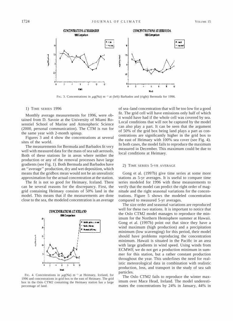
FIG. 3. Concentrations in mg(Na) m23 at (left) Barbados and (right) Bermuda for 1996.

FIG. 4. Concentrations in mg(Na) m23 at Heimaey, Iceland, for1996 and concentrations in grid box to the east of Heimaey. The gridbox in the Oslo CTM2 containing the Heimaey station has a largepercentage of land.

1) TIME SERIES 1996

Monthly average measurements for 1996, were ob-tained from D. Savoie at the University of Miami Ro-senstiel School of Marine and Atmospheric Science(2000, personal communication). The CTM is run forthe same year with 2-month spinup.

Figures 3 and 4 show the concentrations at severalsites of the world.

The measurements for Bermuda and Barbados fit verywell with measured data for the mass of sea salt aerosols.Both of these stations lie in areas where neither theproduction or any of the removal processes have largegradients (see Fig. 1). Both Bermuda and Barbados havean ‘‘average’’ production, dry and wet deposition, whichmeans that the gridbox mean would not be an unrealisticapproximation for the actual concentration at the station.

The fit is not so good for Heimaey, Iceland. Therecan be several reasons for the discrepancy. First, thegrid containing Heimaey consists of 50% land in themodel. This means that if the measurements are doneclose to the sea, the modeled concentration is an average

of sea–land concentration that will be too low for a goodfit. The grid cell will have emissions only half of whichit would have had if the whole cell was covered by sea.Local conditions that will not be captured by the modelcan also play a part. It can be seen that the argumentof 50% of the grid box being land plays a part as con-centrations are significantly higher in the grid box tothe east of Heimaey with 100% sea cover (see Fig. 4).In both cases, the model fails to reproduce the maximummeasured in December. This maximum could be due tolocal conditions at Heimaey.

2) TIME SERIES 5-YR AVERAGE

Gong et al. (1997b) give time series at some morestations as 5-yr averages. It is useful to compare timeseries modeled for 1996 with these measurements toverify that the model can predict the right order of mag-nitude and the right seasonal variations for the concen-trations. Figure 5 shows the modeled concentrationcompared to measured 5-yr averages.

The size order and seasonal variations are reproducedwell for these two stations. It is important to notice thatthe Oslo CTM2 model manages to reproduce the min-imum for the Northern Hemisphere summer at Hawaii.Gong et al. (1997b) point out that since they have awind maximum (high production) and a precipitationminimum (low scavenging) for this period, their modelshould have problems reproducing the concentrationminimum. Hawaii is situated in the Pacific in an areawith large gradients in wind speed. Using winds fromECMWF, we do not get a production minimum in sum-mer for this station, but a rather constant productionthroughout the year. This underlines the need for real-istic meteorological data in combination with realisticproduction, loss, and transport in the study of sea saltparticles.

The Oslo CTM2 fails to reproduce the winter max-imum over Mace Head, Ireland. The model underesti-mates the concentrations by 24% in January, 44% in

1 JULY 2002 1725G R I N I E T A L .

FIG. 5. Concentrations in mg(Na) m23 (5-yr averages) for (left) Hawaii, United States, and (right)Mace Head, Ireland, compared to model results for 1996.

TABLE 4. Yearly averaged standard deviation from measuredvalues for different stations.

Station Std dev (%)

BarbadosBermudaHawaiiMace Head

15.915.715.627.0

February, and 48% in March. This could be a result oflocal conditions similar to those discussed above forHeimaey. It can also be seen that the modeled results(1996) show more variation than the 5-yr mean curvethat is smoother. It is normal that calculations for oneparticular year deviate from a 5-yr average.

In Table 4, some average standard deviations for themonthly mean time series are shown. The deviation iscalculated for each month and then averaged for thewhole year. Heimaey is not included for reasons dis-cussed above.

3) WEEKLY AVERAGES

At some stations, we have compared weekly averagesmeasured from 1996 to weekly averages from the mod-el. This should give an indication if the dependence onmeteorology (e.g., wind, rainfall) is correct. The vari-ations should correspond not only seasonally, but alsoon shorter timescales.

Figure 6 shows weekly averages for two stations dur-ing the first few weeks of 1996. The modeled variationsseem to follow the observations nicely. The model con-centrations covary with the measured concentrations.

At the Reunion Island site we have quite large weeklyvariations, something that is reproduced by the model.The model generally overestimates the concentrations atthis site with a minimum overestimation of 18% in week6 and a maximum overestimation of 470% in week 5.

At the Chatman Island site where the measurements

show low variance, the model shows low variance aswell. At this site, the model generally overestimates theconcentrations. The model overestimates by 52% inweek 1, 60% in week 4, and 76% in week 8, but forsome weeks, the model underestimates the concentra-tions, such as in week 3 (12%) and week 5 (31%).

4) SIZE DISTRIBUTIONS

The mass size distributions at selected stations areshown in Fig. 7.

The size distribution is expected to be lognormal. Inthis case, we get a bimodal distribution with anothermaximum at about r 5 10 mm because of the contri-bution of spume particles to the production.

Erickson and Duce (1988) propose that the distri-bution fitted to lognormality should be distributed aboutthe radius r 5 0.422u 1 2.12 where u is surface windspeed. This would mean that for a surface wind speedof 10 m s21, the distribution would be lognormally dis-tributed around r 5 6 mm. The actual measured massmedian radius from the work of Erickson and Duce(1988) varied between 3.5 and 7.5 mm. They do notgive any standard variation. Seinfeld and Pandis (1998)also propose that marine background aerosols are log-normally distributed around r 5 6 mm. The Oslo CTM2approximately reproduces this size distribution.

5) VARIATION WITH HEIGHT

Mass concentrations decrease with height. The lossterms that lead to this are the falling velocity and thescavenging. The variation of total mass with height isshown in Fig. 8.

We do not get significant transport of sea salt massto higher altitudes in the troposphere. The zonal meanor aerosol mass is high at latitudes with high wind andhigh ocean fraction. The washout process removes anysea salt that is transported to higher altitudes, therefore

1726 VOLUME 15J O U R N A L O F C L I M A T E

FIG. 6. Weekly averages for surface level concentrations in mg(Na) m23 at (left) Chatman Islandand (right) Reunion Island for 1996.

FIG. 7. Modeled size distribution for (left) Barbados and (right) Mace Head, Ireland. Radius is at80% relative humidity.

no significant amount of sea salt mass is found over 750hPa.

The high concentrations at 608S is a consequence ofhigh wind speeds, and small land fraction at this latitude.

The mass of different size bins vary differently withheight. The larger particles have a higher falling veloc-ity, and the concentration of these particles decreasemore rapidly with altitude than the mass of the smallerparticles. Figure 9 shows the concentration as a functionof height at two stations.

At Heimaey in January, where washout is expectedto be efficient, we see a more rapid decrease in con-centrations with height than at Hawaii where washoutis expected to be less efficient. The vertical profile isalso influenced by different production (of different siz-es of particles) or differences in transport.

We have made a global average column of the mod-eled results. The concentrations have been approximatedto a formula of the form C 5 C0e2Z/H where C is con-centration in mg m23, Z is altitude, and H is scale height(both measured in km). There are two distinguishedregimes with H 5 1 km below approximately 2 km and

H 5 5.5 km above approximately 2 km. For comparison,Koepke et al. (1997) used scale heights of 1 and 8 kmfor the two regions. This means that our model containsless sea salt mass in the free troposphere.

c. Radiative impact

In this section we will use the term radiative forcingof the radiative impact of sea salt. Usually radiativeforcing is used for an external perturbation (anthropo-genic or natural perturbation such as solar irradiationvariation or aerosols from volcanic eruptions; Houghtonet al. 1996); however, here we use the term radiativeforcing for a natural component.

Results are performed with clouds included and forclear sky (clouds excluded in the calculations). Resultsfor clear sky are presented first as these are most com-parable to the results from Haywood et al. (1999) andBoucher and Tanre (2000), which are combinations ofsatellite observation and modeling. However, note thatsatellite observations are only performed for clear sky

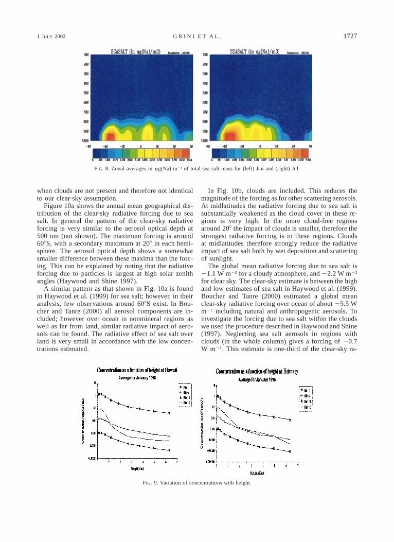
1 JULY 2002 1727G R I N I E T A L .

FIG. 8. Zonal averages in mg(Na) m23 of total sea salt mass for (left) Jan and (right) Jul.

FIG. 9. Variation of concentrations with height.

when clouds are not present and therefore not identicalto our clear-sky assumption.

Figure 10a shows the annual mean geographical dis-tribution of the clear-sky radiative forcing due to seasalt. In general the pattern of the clear-sky radiativeforcing is very similar to the aerosol optical depth at500 nm (not shown). The maximum forcing is around608S, with a secondary maximum at 208 in each hemi-sphere. The aerosol optical depth shows a somewhatsmaller difference between these maxima than the forc-ing. This can be explained by noting that the radiativeforcing due to particles is largest at high solar zenithangles (Haywood and Shine 1997).

A similar pattern as that shown in Fig. 10a is foundin Haywood et al. (1999) for sea salt; however, in theiranalysis, few observations around 608S exist. In Bou-cher and Tanre (2000) all aerosol components are in-cluded; however over ocean in nonmineral regions aswell as far from land, similar radiative impact of aero-sols can be found. The radiative effect of sea salt overland is very small in accordance with the low concen-trations estimated.

In Fig. 10b, clouds are included. This reduces themagnitude of the forcing as for other scattering aerosols.At midlatitudes the radiative forcing due to sea salt issubstantially weakened as the cloud cover in these re-gions is very high. In the more cloud-free regionsaround 208 the impact of clouds is smaller, therefore thestrongest radiative forcing is in these regions. Cloudsat midlatitudes therefore strongly reduce the radiativeimpact of sea salt both by wet deposition and scatteringof sunlight.

The global mean radiative forcing due to sea salt is21.1 W m22 for a cloudy atmosphere, and 22.2 W m22

for clear sky. The clear-sky estimate is between the highand low estimates of sea salt in Haywood et al. (1999).Boucher and Tanre (2000) estimated a global meanclear-sky radiative forcing over ocean of about 25.5 Wm22 including natural and anthropogenic aerosols. Toinvestigate the forcing due to sea salt within the cloudswe used the procedure described in Haywood and Shine(1997). Neglecting sea salt aerosols in regions withclouds (in the whole column) gives a forcing of 20.7W m22. This estimate is one-third of the clear-sky ra-

1728 VOLUME 15J O U R N A L O F C L I M A T E

FIG. 10. Yearly averaged direct radiative forcing due to sea salt in (a) clear-sky conditions and(b) taking clouds into account.

diative forcing, a result that shows that clouds are veryoften present in regions with sea salt. We find a forcingof 20.4 W m22 inside cloudy regions or 35% of theradiative forcing.

Normalized forcing (global mean radiative forcingdivided by the global mean burden) has been calculatedby many investigators for sulfate aerosols (see Myhreet al. 1998, and references therein). It ranges from about2550 to 2125 W g21. For mineral dust the normalizedforcing range from 211 to 14 W g21 in Myhre andStordal (2001). In the calculations performed in thisstudy the normalized forcing for sea salt is 288 W g21.The lower normalized forcing for sea salt aerosols thanfor sulfate is mainly due to larger sizes of the sea saltaerosols. Mineral aerosols also have large sizes like thesea salt particles. In addition they absorb solar radiationand have a significant thermal infrared radiative forcingleading to small normalized forcing for mineral aero-sols.

We have performed two additional calculations inwhich we have reduced the number of size bins from16 to 8 and 4. Differences in results when the numberof size bins are reduced may have several origins. This

will influence the dry deposition as the dry depositionshows a strong, nonlinear variation with the radius(Seinfeld and Pandis 1998), and the total burden ischanged. Further, the optical properties may change ei-ther as a result of change in the calculated size distri-bution or simply in the averaging procedure in the cal-culation of the optical properties. Reducing the numberof size bins from 16 to 8 decreases the radiative forcingonly by 4%. However, as the total burden is slightlyincreased (2%), the normalized forcing is reduced by6%. When four size bins are used, larger changes occur.The radiative forcing is 7% stronger, whereas the totalburden is 23% higher, giving a normalized forcing thatis 13% lower. The scattering efficiency for aerosols isstrongly dependent on the size of the aerosols. In thevisible region the scattering efficiency has a strong max-imum for aerosols with radius around 0.5 mm (see, e.g.,Seinfeld and Pandis 1998). This nonlinear variation inthe scattering efficiency leads to an underestimation ofthe radiative forcing for 4 and 8 size classes comparedto 16 size classes. However, larger differences in theburden is found, mainly because of averaging the drydeposition over larger size intervals.

1 JULY 2002 1729G R I N I E T A L .

4. Summary

A global 3D CTM (the Oslo CTM2) has been usedto simulate the concentration of sea salt particles in theatmosphere. The distribution is determined by produc-tion (generation by wind), transport (advection and con-vection), wet and dry deposition, and growth by con-densation. This study calculates the fluxes of sea salt asa function of wind speed. Earlier studies have eithercalculated sea salt concentrations in the boundary layerdirectly from empirical wind speed correlations or usedless-sophisticated models (e.g., 1D models).

Monthly averaged distributions have been comparedwith measurements from Hawaii, Barbados, Bermuda,Ireland, and Iceland, and with weekly averages fromChatman Island and the Reunion Island. The calculatedsurface concentrations vary between 0 and 16 mg(Na)m23 and fit well with the measured values.

The global flux of sea salt is calculated to be 6500Tg yr21. Earlier estimates lie between 1000 and 10 000Tg yr21. Average burden of sea salt is calculated to 12mg m22, which is within the range of earlier estimatesthat are between 7.5 and 36 mg m22. Global averageradiative forcing of sea salt is estimated to 21.1 W m22

when the effect of clouds is taken into account and 22.2W m22 when the effect of clouds is ignored. It is im-portant to take the effect of clouds into account in aconsistent way using the same meteorology to calculateemissions, transport, and radiative forcing, since the seasalt concentrations often are high in areas with extensivecloud cover.

Acknowledgments. We are grateful to Prof. David Sa-voie for providing his measurements of sea salt particles.They were important for validating the model results.This work has been sponsored by the Norwegian Re-search Council through Grant 139810/720 (CHEM-CLIM).

REFERENCES

Bergstrom, R., and P. Russel, 1999: Estimation of aerosol directradiative effects over the mid-latitude North Atlantic fromsatellite and in situ measurements. Geophys. Res. Lett., 26,1731–1734.

Blanchard, D., 1985: The oceanic production of atmospheric sea salt.J. Geophys. Res., 90, 961–963.

Boucher, P., and D. Tanre, 2000: Estimation of the aerosol perturbationto the earth’s radiative budget over oceans using polder satelliteaerosol retrievals. Geophys. Res. Lett., 27, 1103–1106.

Erickson, D. J., and R. A. Duce, 1988: On global flux of atmosphericsea salt. J. Geophys. Res., 93, 14 079–14 088.

Fitzgerald, J. W., 1975: Approximation formula for the equilibriumsize of an aerosol particle as a function of its dry size andcomposition and the ambient relative humidity. J. Appl. Meteor.,14, 1044–1049.

Gong, S. L., L. A. Barrie, and J.-P. Blanchet, 1997a: Modeling sea-salt aerosols in the atmosphere. 1: Model development. J. Geo-phys. Res., 102, 3805–3818.

——, ——, J. M. Prospero, D. L. Savoie, G. P. Ayers, J.-P. Blanchet,and L. Spacek, 1997b: Modeling sea-salt aerosols in the atmo-

sphere. 2: Atmospheric concentration and fluxes. J. Geophys.Res., 102, 3819–3830.

Haywood, J., and K. Shine, 1997: Multi-spectral calculations of thedirect radiative forcing of tropospheric sulphate and soot aerosolsusing a column model. Quart. J. Roy. Meteor. Soc., 123, 1907–1930.

——, and O. Boucher, 2000: Estimates of the direct and indirectradiative forcing due to tropospheric aerosols: A review. Rev.Geophys., 38, 513–543.

——, V. Ramaswamy, and B. Soden, 1999: Tropospheric aerosolclimate forcing in clear sky satellite observation over the oceans.Science, 283, 1299–1303.

Hess, M., P. Koepke, and I. Schult, 1998: Optical properties of aero-sols and clouds: The software package OPAC. Bull. Amer. Me-teor. Soc., 79, 831–844.

Hogan, R. J., and A. J. Illingsworth, 2000: Deriving cloud overlapstatistics from radar. Quart. J. Roy. Meteor. Soc., 126, 2903–2909.

Houghton, J. T., L. G. Meira Filho, B. A. Callander, N. Harris, A.Kattenberg, and K. Maskell, Eds.,1996: Climate Change 1995:The Science of Climate Change. Cambridge University Press,572 pp.

King, M., Y. Kaufman, D. Tanre, and T. Nakajima, 1999: Remotesensing of tropospheric aerosols from space: Past, present, andfuture. Bull. Amer. Meteor. Soc., 80, 2229–2259.

Koepke, P., M. Hess, I. Schult, and E. Shettle, 1997: Global aerosoldata set. Max Planck Institute for Meteorology Tech. Rep. 243,Hamburg, Germany, 50 pp.

Monahan, E., D. Spiel, and K. Spiel, 1986: Oceanic Whitecaps. Rei-del.

Myhre, G., and F. Stordal, 2001: Global sensitivity experiments ofthe radiative forcing due to mineral aerosols. J. Geophys. Res.,106 (D16), 18 193–18 204.

——, ——, K. Restad, and I. Isaksen, 1998: Estimates of the directradiative forcing due to sulfate and soot aerosols. Tellus, 50B,463–477.

Petrenchuk, O. P., 1980: On the budget of sea salts and sulphur inthe atmosphere. J. Geophys. Res., 85, 7439–7444.

Prather, M. J., 1986: Numerical advection by conservation of second-order moments. J. Geophys. Res., 91, 6671–6681.

Pryor, S. C., and L. L. Sorensen, 2000: Nitric acid–sea salt reactions:Implications for nitrogen deposition to water surfaces. J. Appl.Meteor., 39, 725–731.

Seinfeld, J. H., and S. N. Pandis, 1998: Atmospheric Chemistry andPhysics, From Air Pollution to Climate Change. John Wiley andSons, 1326 pp.

Shettle, E., and R. Fenn, 1979: Models for the aerosols of the loweratmosphere and the effects of humidity variations on their opticalproperties. AFGL Tech. Rep. TR-79-0214.

Slingo, A., 1989: A GCM parameterization for the shortwave radi-ative properties of water clouds. J. Atmos. Sci., 46, 1419–1427.

Smith, M. H., P. M. Park, and I. E. Consterdine, 1993: Marine aerosolconcentration and estimated fluxes over sea. Quart. J. Roy. Me-teor. Soc., 119, 809–824.

Stamnes, K., S. Tsay, W. Wiscombe, and K. Jayaweera, 1988: Anumerically stable algorithm for discrete-ordinate method ra-diative transfer in multiple scattering and emitting layered media.Appl. Opt., 27, 2502–2509.

Stephens, G., 1978: Radiation profiles in extended water clouds. I:Theory. J. Atmos. Sci., 35, 2111–2122.

——, and C. Platt, 1987: Aircraft observations of the radiative andmicrophysical properties of stratocumulus and cumulus cloudfields. J. Climate Appl. Meteor., 26, 1243–1269.

Sundet, J. K., 1997: Model studies with a 3-d global CTM usingECMWF data. Ph.D. thesis, University of Oslo, Oslo, Norway,102 pp.

Takemura, T., H. Okamoto, Y. Maruyama, A. Numaguti, A. Higurashi,and T. Nakajima, 2000: Global three-dimensional simulation of

1730 VOLUME 15J O U R N A L O F C L I M A T E

aerosol optical thickness distribution of various origins. J. Geo-phys. Res., 105, 17 853–17 873.

Tegen, I., P. Hollrig, M. Chin, I. Fung, D. Jacob, and J. Penner, 1997:Contribution of different aerosol species to the global aerosolextinction optical thickness: Estimates from model results. J.Geophys. Res., 102, 23 895–23 915.

Tiedtke, M., 1989: A comprehensive mass flux scheme for cumulusparameterization on large scale models. Mon. Wea. Rev., 117,1779–1800.

Wiscombe, W., 1980: Improved mie scattering algorithms. Appl. Opt.,19, 1505–1509.

——, and J. Evans, 1977: Exponential sum fitting of radiative trans-mission functions. J. Comput. Physiol., 24, 416–444.

Zhang, Y., C. Seigneur, J. Seinfeld, M. Jacobson, S. Clegg, and F.Binkowski, 2000: A comparative review of inorganic aerosolthermodynamic equilibrium modules: Similarities, differences,and their likely causes. Atmos. Environ., 34, 117–137.