Bayesian Learning

YZM 3226 – Makine Öğrenmesi

Outline

◘ Introduction to Bayesian Learning

◘ Features of Bayesian Learning

◘ Probability Theory

◘ Bayes Theory

◘ Bayesian Classification

◘ Bayesian Learning Examples

◘ Advantages / Disadvantages of Bayesian Learning

Who is he?

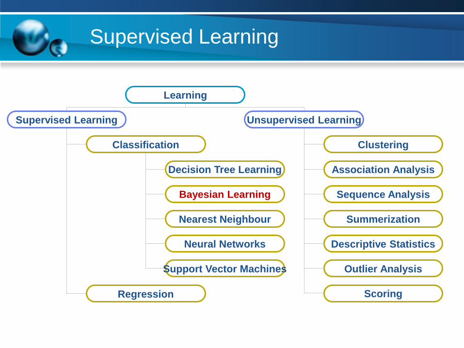
Supervised Learning

Learning

Supervised Learning Unsupervised Learning

Classification

Regression

Clustering

Association AnalysisDecision Tree Learning

Bayesian Learning

Nearest Neighbour

Neural Networks

Support Vector Machines

Sequence Analysis

Summerization

Descriptive Statistics

Outlier Analysis

Scoring

Probability

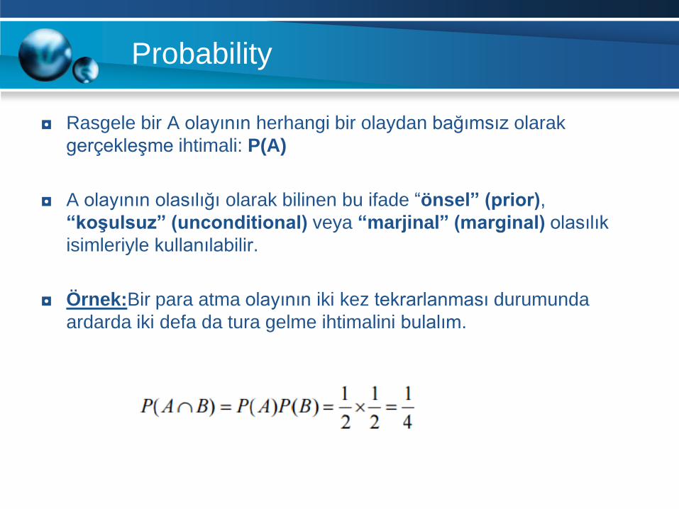
◘ Rasgele bir A olayının herhangi bir olaydan bağımsız olarak

gerçekleşme ihtimali: P(A)

◘ A olayının olasılığı olarak bilinen bu ifade “önsel” (prior),

“koşulsuz” (unconditional) veya “marjinal” (marginal) olasılık

isimleriyle kullanılabilir.

◘ Örnek:Bir para atma olayının iki kez tekrarlanması durumunda

ardarda iki defa da tura gelme ihtimalini bulalım.

Conditional Probability

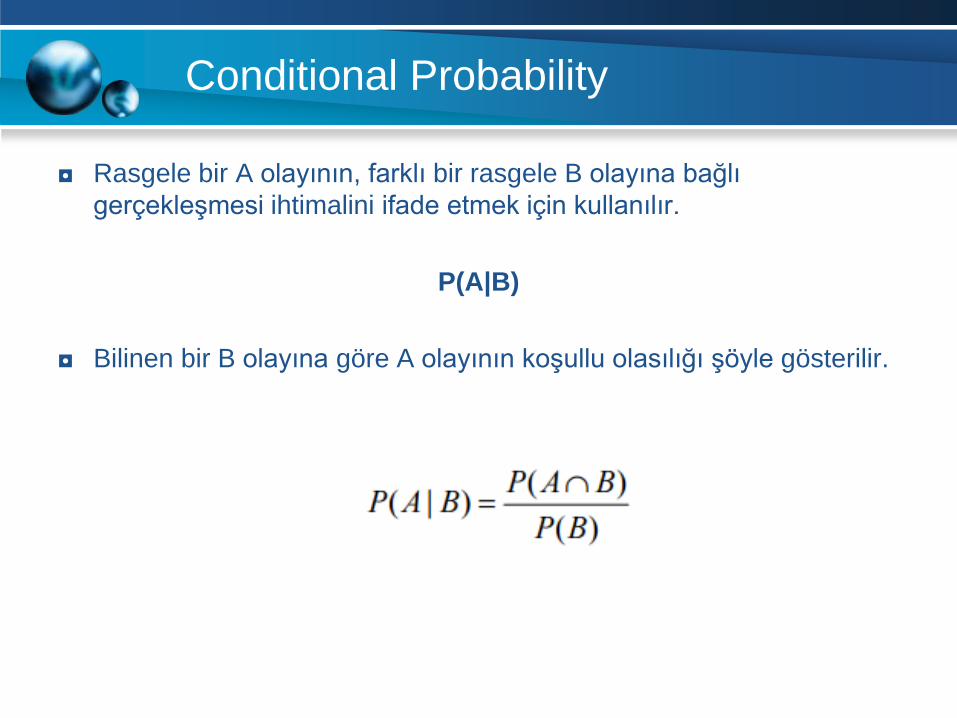
◘ Rasgele bir A olayının, farklı bir rasgele B olayına bağlı

gerçekleşmesi ihtimalini ifade etmek için kullanılır.

P(A|B)

◘ Bilinen bir B olayına göre A olayının koşullu olasılığı şöyle gösterilir.

Example

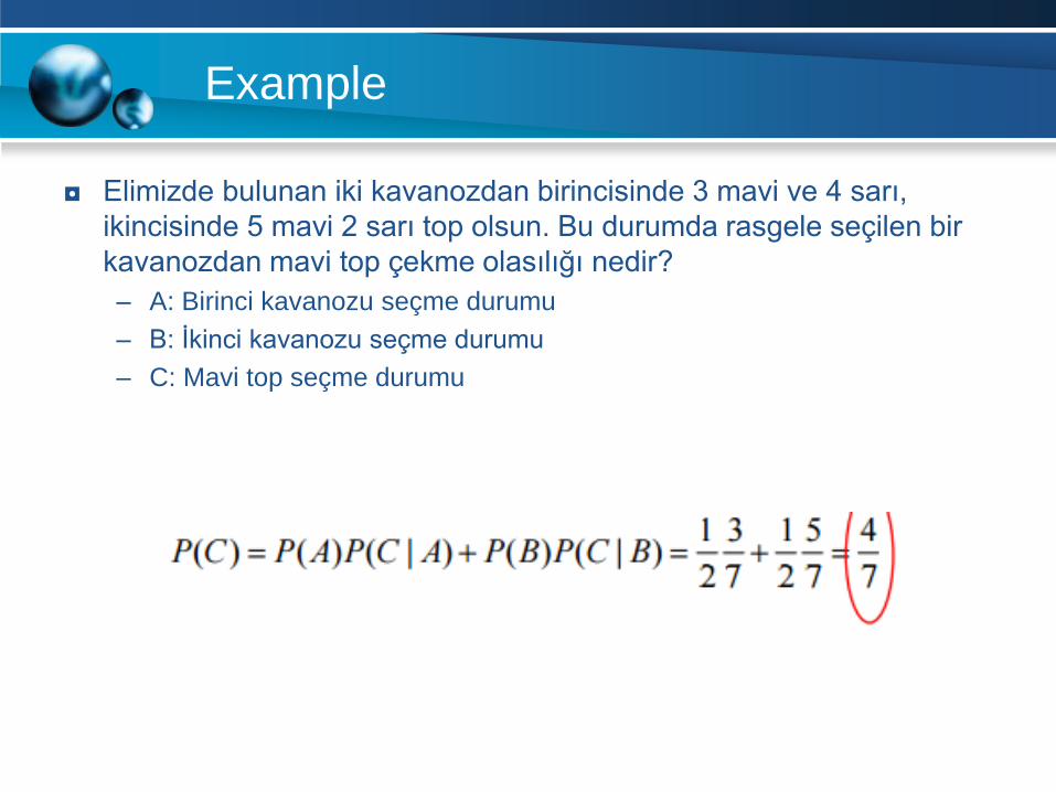
◘ Elimizde bulunan iki kavanozdan birincisinde 3 mavi ve 4 sarı,

ikincisinde 5 mavi 2 sarı top olsun. Bu durumda rasgele seçilen bir

kavanozdan mavi top çekme olasılığı nedir?

– A: Birinci kavanozu seçme durumu

– B: İkinci kavanozu seçme durumu

– C: Mavi top seçme durumu

Bayes Theorem (1/2)

To determine the most probable hypothesis, given the data D plus any initial knowledge about the prior probabilities of the various hypotheses in H.

◘ Prior probability of h, P(h): it reflects any background knowledge we have about the chance that h is a correct hypothesis (before having observed the data).

◘ Prior probability of D, P(D): it reflects the probability that training data D will be observed given no knowledge about which hypothesis h holds.

◘ Conditional Probability of observation D, P(D|h): it denotes the probability of observing data D given some world in which hypothesis hholds.

◘ Posterior probability of h, P(h|D): it represents the probability that hholds given the observed training data D. It reflects our confidence that h holds after we have seen the training data D and it is the quantity that Machine Learning researchers are interested in.

)(

)()|()|(

DP

hPhDPDhP

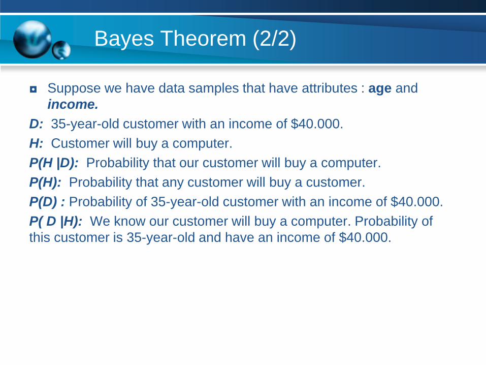
Bayes Theorem (2/2)

◘ Suppose we have data samples that have attributes : age and

income.

D: 35-year-old customer with an income of $40.000.

H: Customer will buy a computer.

P(H |D): Probability that our customer will buy a computer.

P(H): Probability that any customer will buy a customer.

P(D) : Probability of 35-year-old customer with an income of $40.000.

P( D |H): We know our customer will buy a computer. Probability of

this customer is 35-year-old and have an income of $40.000.

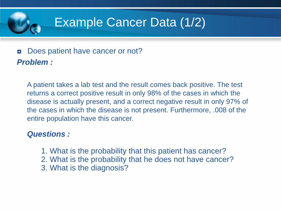
Example Cancer Data (1/2)

◘ Does patient have cancer or not?

Problem :

A patient takes a lab test and the result comes back positive. The test

returns a correct positive result in only 98% of the cases in which the

disease is actually present, and a correct negative result in only 97% of

the cases in which the disease is not present. Furthermore, .008 of the

entire population have this cancer.

Questions :

1. What is the probability that this patient has cancer?2. What is the probability that he does not have cancer?3. What is the diagnosis?

Example Cancer Data (2/2)

– P(cancer)=0.008 P(¬cancer)=0.992

– P(+|cancer)=0.98 P(-|cancer)=0.02

– P(+|¬cancer)=0.03 P(-|¬cancer)=0.97

1) P(+|cancer)P(cancer)=0.98*0.008=0.0078

2) P(+|¬cancer)P(¬cancer)=0.03*0.992=0.0298

3) P( cancer| ) < P(¬cancer| )

Diagnosis : Not cancer

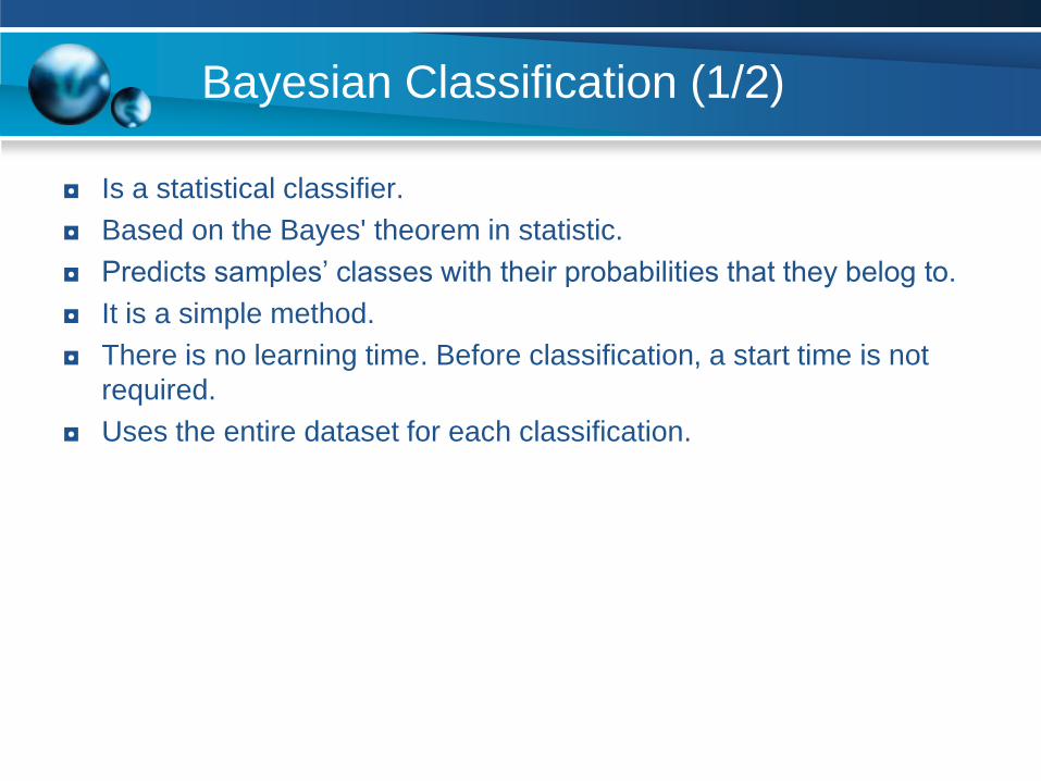
Bayesian Classification (1/2)

◘ Is a statistical classifier.

◘ Based on the Bayes' theorem in statistic.

◘ Predicts samples’ classes with their probabilities that they belog to.

◘ It is a simple method.

◘ There is no learning time. Before classification, a start time is not

required.

◘ Uses the entire dataset for each classification.

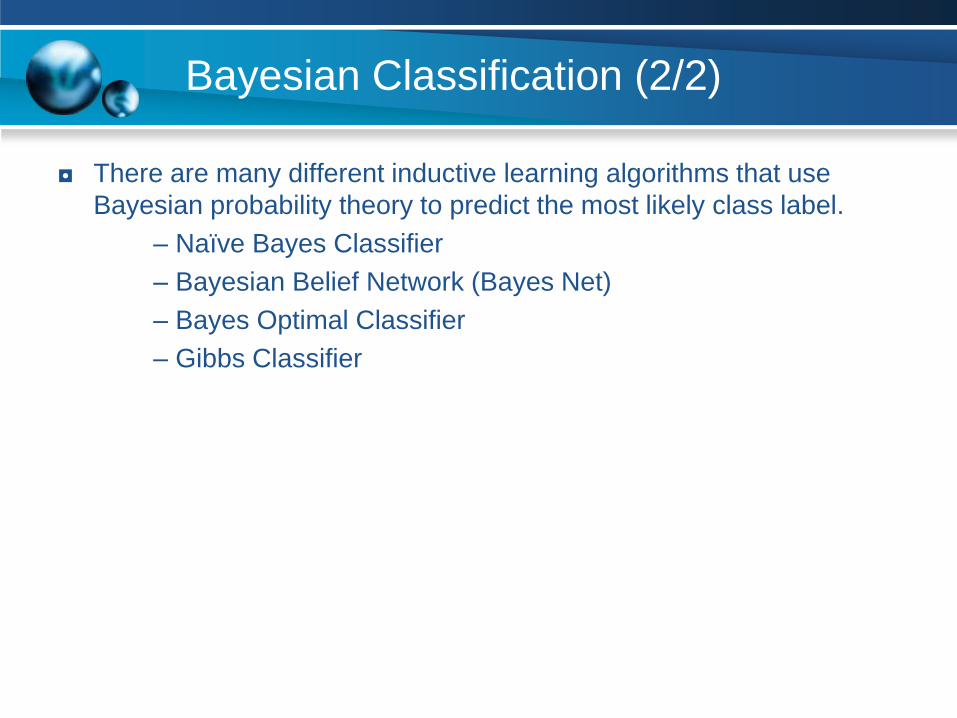
Bayesian Classification (2/2)

◘ There are many different inductive learning algorithms that use

Bayesian probability theory to predict the most likely class label.

– Naïve Bayes Classifier

– Bayesian Belief Network (Bayes Net)

– Bayes Optimal Classifier

– Gibbs Classifier

The Naïve Bayes Classifier

In Bayes Theorem example, we use only one attribute data to

diagnose patient. What can we do if our data d has several attributes?

Naïve Bayes assumption: Attributes that describe data instances are

conditionally independent given the classification hypothesis.

◘ One of the most practical learning methods

◘ Successful applications:

– Medical Diagnosis

– Text classification

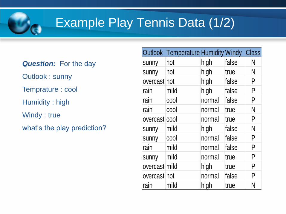
Example Play Tennis Data (1/2)

Outlook Temperature Humidity Windy Class

sunny hot high false N

sunny hot high true N

overcast hot high false P

rain mild high false P

rain cool normal false P

rain cool normal true N

overcast cool normal true P

sunny mild high false N

sunny cool normal false P

rain mild normal false P

sunny mild normal true P

overcast mild high true P

overcast hot normal false P

rain mild high true N

Question: For the day

Outlook : sunny

Temprature : cool

Humidity : high

Windy : true

what’s the play prediction?

Example Play Tennis Data (2/2)

P(yes) =

9/14

P(no) =

5/14

0206.)|()|()|()|()(

0053.)|()|()|()|()(

notruePnohighPnocoolPnosunnypnoP

yestruePyeshighPyescoolPyessunnyPyesP

Thus, the naïve Bayes classifier assigns the value

not PlayTennis!

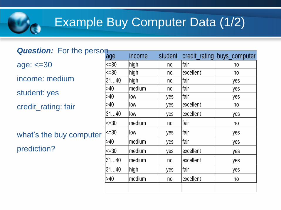
Example Buy Computer Data (1/2)

age income student credit_rating buys_computer<=30 high no fair no

<=30 high no excellent no

31…40 high no fair yes

>40 medium no fair yes

>40 low yes fair yes

>40 low yes excellent no

31…40 low yes excellent yes

<=30 medium no fair no

<=30 low yes fair yes

>40 medium yes fair yes

<=30 medium yes excellent yes

31…40 medium no excellent yes

31…40 high yes fair yes

>40 medium no excellent no

Question: For the person

age: <=30

income: medium

student: yes

credit_rating: fair

what’s the buy computer

prediction?

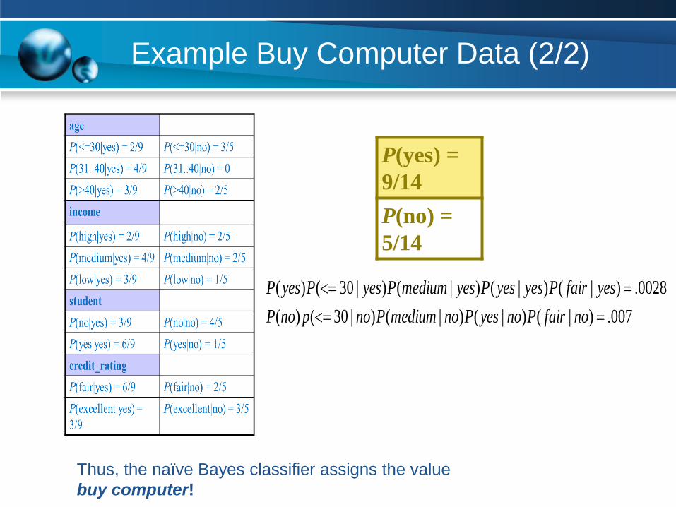
Example Buy Computer Data (2/2)

P(yes) =

9/14

P(no) =

5/14

007.)|()|()|()|30()(

0028.)|()|()|()|30()(

nofairPnoyesPnomediumPnopnoP

yesfairPyesyesPyesmediumPyesPyesP

Thus, the naïve Bayes classifier assigns the value

buy computer!

Laplacian Correction (1/3)

The Laplacian correction (or Laplace estimator) is a way of

dealing with zero probability values.

In training set, if there is an attribute value that has zero

probability,it cancels the effects of all of the other posteriori probabilities

on Ci.

There is a simple trick to avoid this problem. We can assume

that our training set is so large that adding one to each count that we

need would only make a negligible difference in the estimated

probabilities, yet would avoid the case of zero probability values. This

technique is know as Laplacian correction. (or Laplace estimator). We

add one sample to each attribute value.

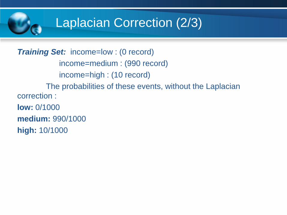
Laplacian Correction (2/3)

Training Set: income=low : (0 record)

income=medium : (990 record)

income=high : (10 record)

The probabilities of these events, without the Laplacian

correction :

low: 0/1000

medium: 990/1000

high: 10/1000

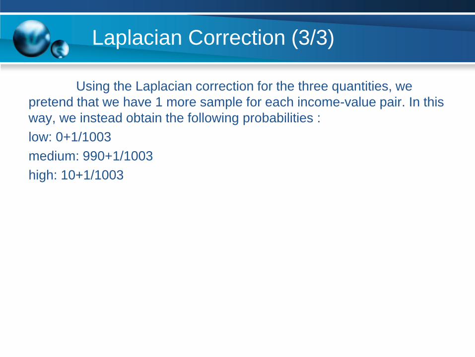
Laplacian Correction (3/3)

Using the Laplacian correction for the three quantities, we

pretend that we have 1 more sample for each income-value pair. In this

way, we instead obtain the following probabilities :

low: 0+1/1003

medium: 990+1/1003

high: 10+1/1003

Continuous Attributes

◘ If Xi is a continuous feature rather than a discrete one, need another

way to calculate P(Xi | Y).

◘ Assume that Xi has a Gaussian distribution whose mean and

variance depends on Y.

◘ During training, for each combination of a continuous feature Xi and

a class value for Y, yk, estimate a mean, μik , and standard deviation

σik based on the values of feature Xi in class yk in the training data.

◘ During testing, estimate P(Xi | Y=yk) for a given example, using the

Gaussian distribution defined by μik and σik .

2

2

2

)(exp

2

1)|(

ik

iki

ik

ki

XyYXP

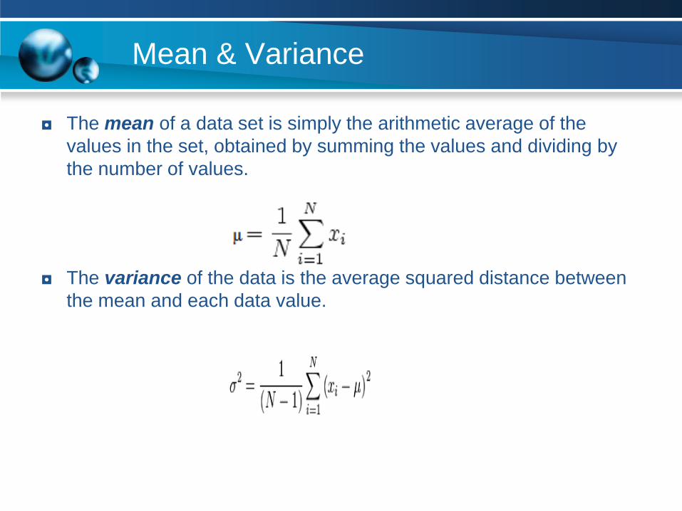
Mean & Variance

◘ The mean of a data set is simply the arithmetic average of the

values in the set, obtained by summing the values and dividing by

the number of values.

◘ The variance of the data is the average squared distance between

the mean and each data value.

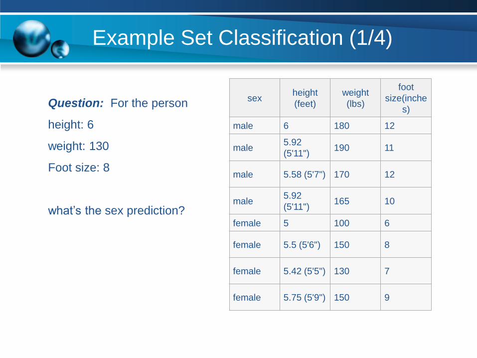
Example Set Classification (1/4)

sexheight

(feet)

weight

(lbs)

foot

size(inche

s)

male 6 180 12

male5.92

(5'11")190 11

male 5.58 (5'7") 170 12

male5.92

(5'11")165 10

female 5 100 6

female 5.5 (5'6") 150 8

female 5.42 (5'5") 130 7

female 5.75 (5'9") 150 9

Question: For the person

height: 6

weight: 130

Foot size: 8

what’s the sex prediction?

Example Set Classification (2/4)

◘ The classifier created from the training set using a Gaussian

distribution assumption would be :

sexmean

(height)

variance

(height)

mean

(weight)

variance

(weight)

mean

(foot

size)

variance

(foot

size)

male 5.8553.5033e-

02176.25

1.2292e

+0211.25

9.1667e-

01

female 5.41759.7225e-

02132.5

5.5833e

+027.5

1.6667e

+00

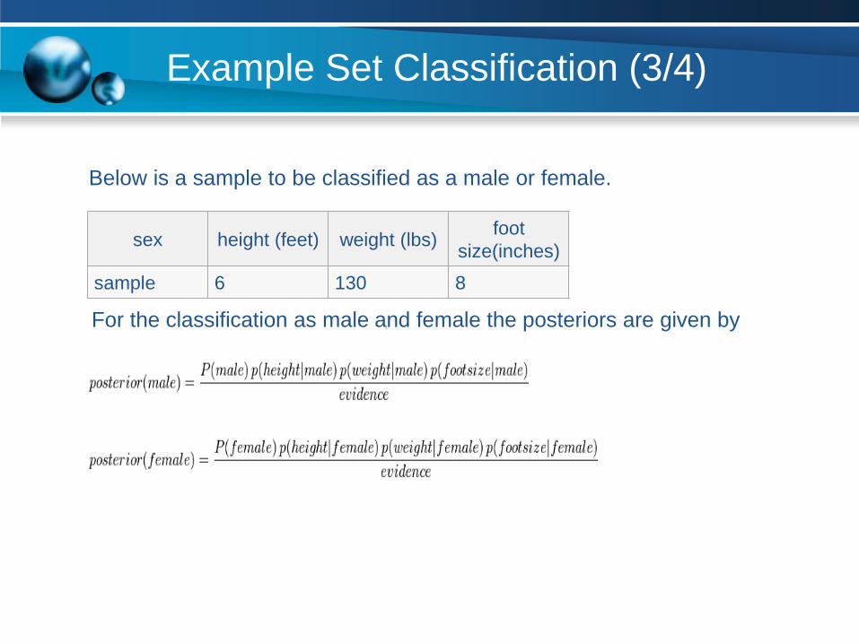
Example Set Classification (3/4)

sex height (feet) weight (lbs)foot

size(inches)

sample 6 130 8

Below is a sample to be classified as a male or female.

For the classification as male and female the posteriors are given by

Example Set Classification (4/4)

We now determine the probability distribution for the sex of the

sample.

where and

are the parameters of normal distribution

which have been previously determined

from the training set.

Since posterior numerator is greater in the female case,

we predict the sample is female.

Multimedia GUIGarb.Coll.SemanticsML Planning

planning

temporal

reasoning

plan

language...

programming

semantics

language

proof...

learning

intelligence

algorithm

reinforcement

network...

garbage

collection

memory

optimization

region...

“planning

language

proof

intelligence

reasoning”

Training

Data:

Test

Data:

Classes:

(AI)

Document Classification with Bayes

(Programming) (HCI)

... ...

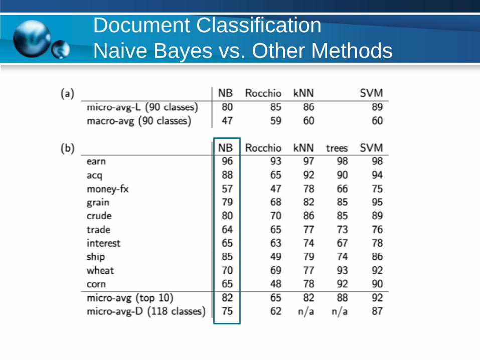
Document Classification

Naive Bayes vs. Other Methods

Advantages and Disadvantages of

Naïve Bayes

◘ Advantages :

Easy to implement

Requires a small amount of training data to estimate

the parameters

Good results obtained in most of the cases

◘ Disadvantages:

Assumption of class conditional independence usually

does not hold

Practically, dependencies exist among variables – E.g., hospitals: patients: Profile: age, family history, etc.

– Symptoms: fever, cough etc., Disease: lung cancer, diabetes, etc.

Dependencies among these cannot be modelled by Naïve

Bayesian Classifier

Bayesian Belief Networks

◘ Also called Bayes Nets

◘ A Bayes net is a model.

◘ It reflects the states of some part of a world that is being modeled

and it describes how those states are related by probabilities.

◘ Allows combining prior knowledge about (in)dependence among

variables with observed training data

Bayesian Belief Networks

◘ Bayesian Networks – graphical probabilistic models

◘ Efficient representation and inference

◘ Expert knowledge + learning from data

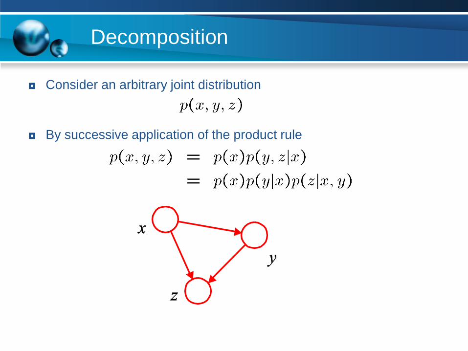
Decomposition

◘ Consider an arbitrary joint distribution

◘ By successive application of the product rule

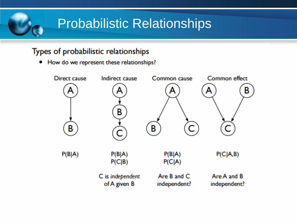
Probabilistic Relationships

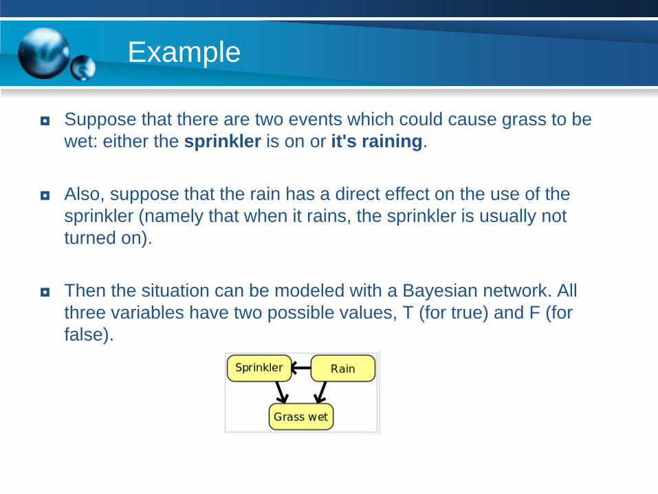
Example

◘ Suppose that there are two events which could cause grass to be

wet: either the sprinkler is on or it's raining.

◘ Also, suppose that the rain has a direct effect on the use of the

sprinkler (namely that when it rains, the sprinkler is usually not

turned on).

◘ Then the situation can be modeled with a Bayesian network. All

three variables have two possible values, T (for true) and F (for

false).

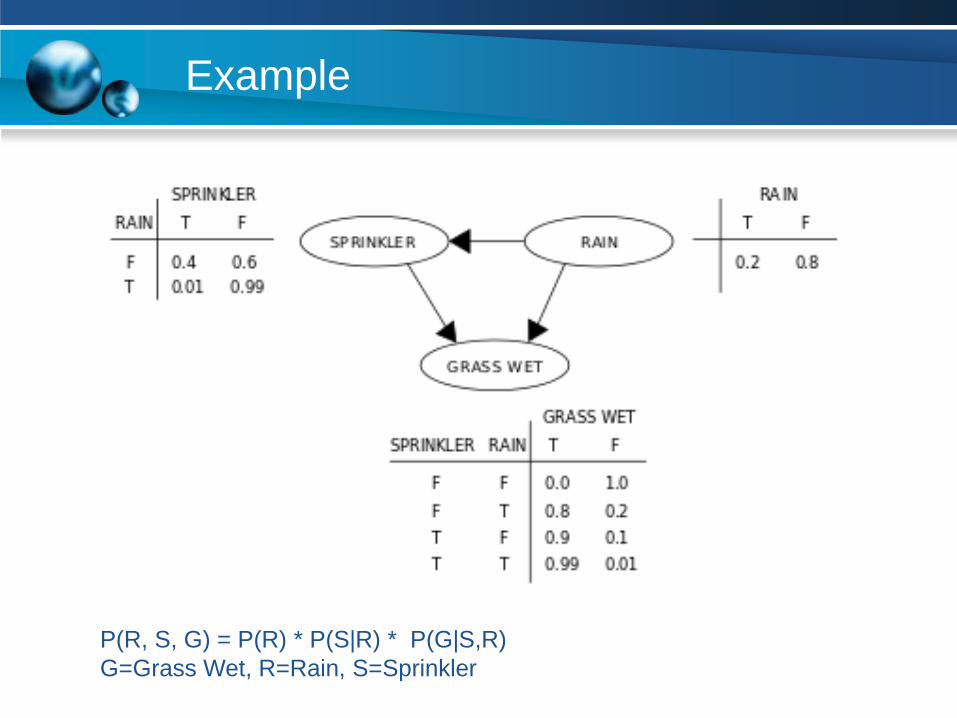
Example

P(R, S, G) = P(R) * P(S|R) * P(G|S,R)

G=Grass Wet, R=Rain, S=Sprinkler

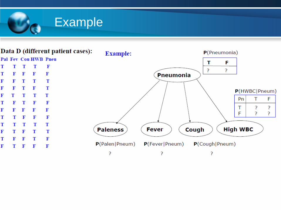
Example

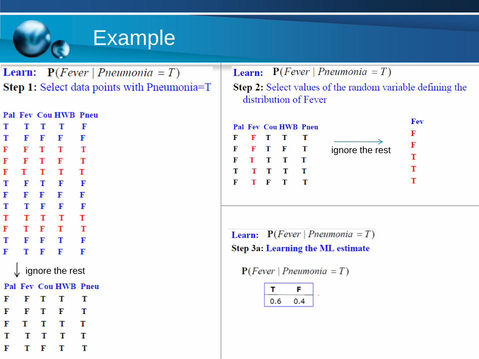
Example

ignore the rest

ignore the rest

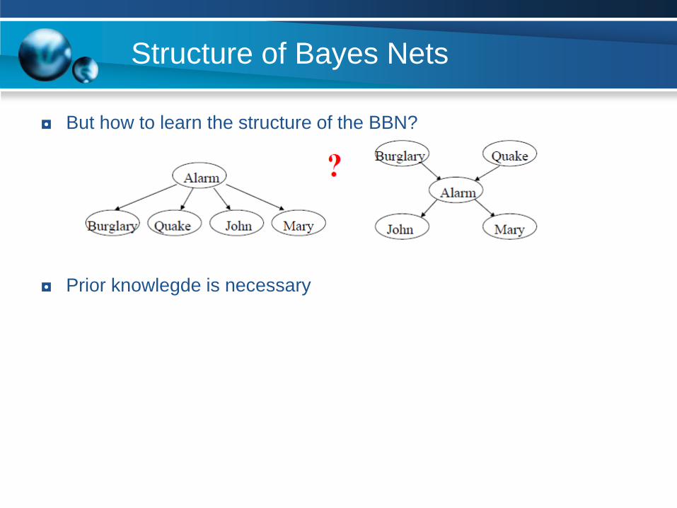
Structure of Bayes Nets

◘ But how to learn the structure of the BBN?

◘ Prior knowlegde is necessary

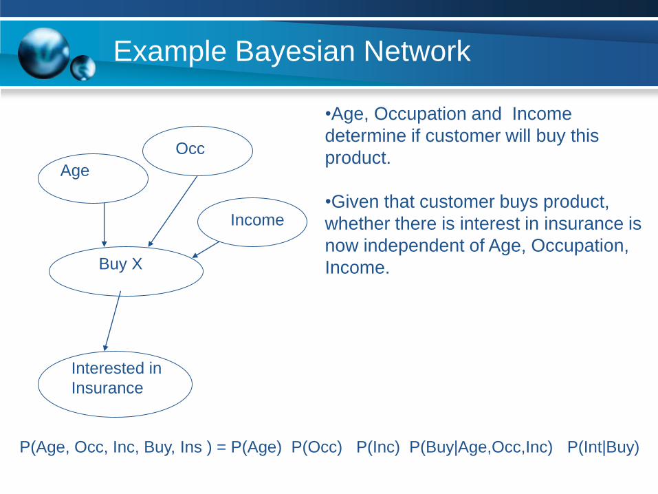
Example Bayesian Network

•Age, Occupation and Income

determine if customer will buy this

product.

•Given that customer buys product,

whether there is interest in insurance is

now independent of Age, Occupation,

Income.

Age

Occ

Income

Buy X

Interested in

Insurance

P(Age, Occ, Inc, Buy, Ins ) = P(Age) P(Occ) P(Inc) P(Buy|Age,Occ,Inc) P(Int|Buy)

Training/Test Split

◘ Randomly split dataset into two parts:

– Training data

– Test data

◘ Use training data to optimize parameters

◘ Evaluate error using test data

◘ After training save model to use future

◘ Classification accuracy depends upon the dimensionality and the

amount of training data

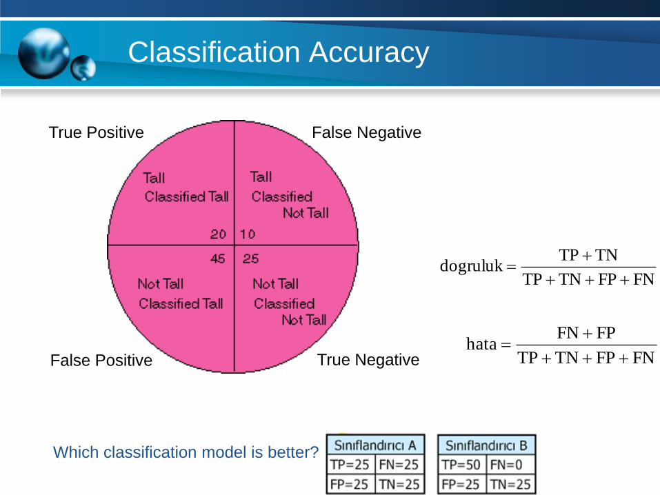
Classification Accuracy

True Positive

True NegativeFalse Positive

False Negative

FNFPTNTP

TNTPdogruluk

FNFPTNTP

FPFNhata

Which classification model is better?

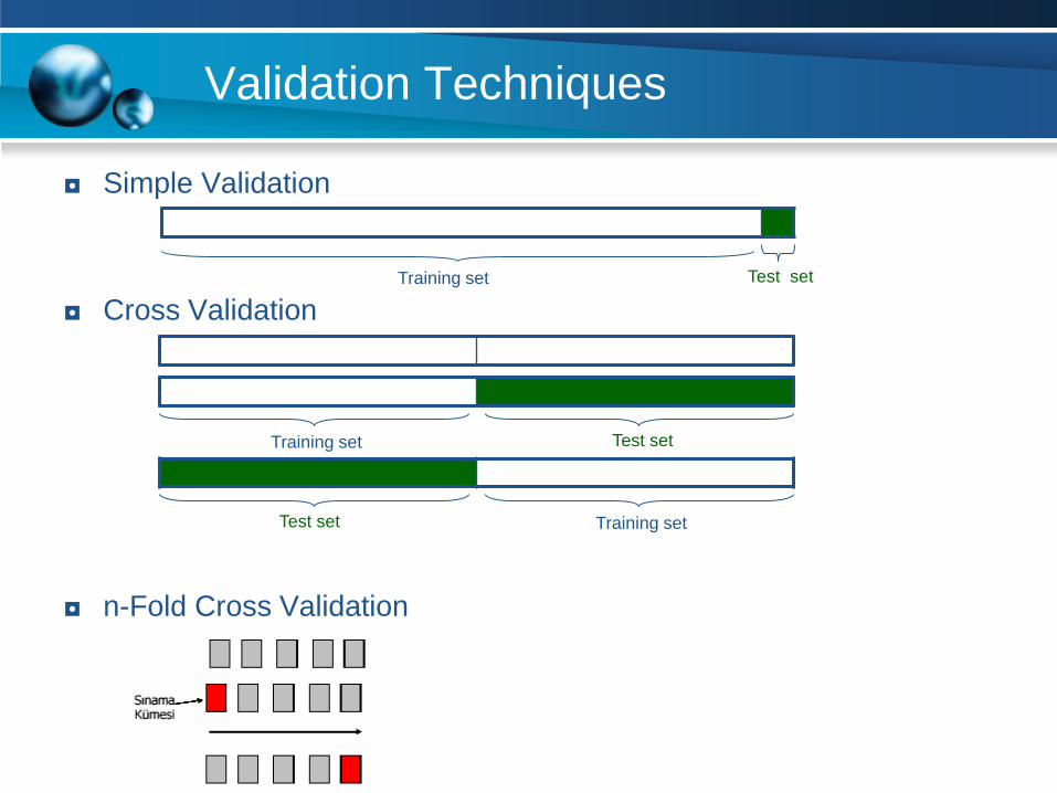
Validation Techniques

◘ Simple Validation

◘ Cross Validation

◘ n-Fold Cross Validation

Training set Test set

Training set Test set

Training setTest set

Summary

◘ Basis for probabilistic learning methods

◘ Naïve Bayes Classifier

– useful in many practical situations

◘ Belief networks

– more expressive representation for conditional independency